Relationship Between Education and GDP Growth: A Bi ... pdf/Events/2011-5th...Relationship Between Education and GDP Growth: A Bi-variate Causality Analysis for Greece M. Solaki1*

Relationship Between Education and GDP Growth: A Bi-variate Causality Analysis for

Greece

M. Solaki

1*

1 PhD Candidate, Harokopio University, Athens Greece

*Corresponding author. Tel +30 2109549361, E-mail: [email protected]

ABSTRACT

The aim of the paper is to investigate the long-run and the short-run relationship

between human capital and economic growth in Greece over the period 1961-2006. The

article uses bi-variate causality analysis, to study dynamics, by employing different methods

of estimation. Specifically, the empirical results suggests that there is a positive relationship

between education and GDPC and that Tertiary Education should be considered as exogenous

variable, which implies that education contributed to economic growth in Greece during the

estimation period.

Keywords: VECM, Granger Causality, Macro-Level Data, Education, Economic Growth.

1. INTRODUCTION

The economic crisis1 combined with the restructuring of Greek educational system

2,

demands the re-examination of the way that human capital is defined. Specifically, Greek

economy has shown some major structural differences during the last 20 years and as a result

the 67% of the labour force to occupy in the section of services, the 19% in the section of

industry and only 9% in the section of agriculture (El. STAT., 2009).

This research tries to fill in the gap for Greece till 2006 and to conclude whether there

are any structural differences. This paper differs from previous studies, since it is capturing

the long-run and the short-run dynamics of this relationship and it‟s testing for its structural

stability.

The purpose of this paper is to examine the long-run relationship between human

capital and economic growth and the causal direction between them, measuring human capital

in terms of quantity. The paper utilizes the technique of the vector error correction models.

This is accomplished in four steps.

First, the stationarity properties of the data and the order of integration are tested.

Second, the Engle-Granger, the Phillips-Hansen co-integration tests and the Johansen

maximum likelihood method are employed to search for co-integration in a education-real

GDP per capita bi-variate model. Third, the vector error correction model is used to indicate

the direction of Granger causality both in the long and short-run. Finally, the stability of the

coefficients in the estimated relations is tested using Cusum and Cusumq tests.

The paper proceeds as follows. Section 2, briefly reviews the theoretical framework

and previews studies. Section 3, presents the methodological issues and the data used in the

empirical analysis Section 4, reports all the empirical results and section 5, contains

concluding remarks and policy implications.

2. THEORETICAL BACKROUND AND LITERATURE REVIEW

The interaction between human capital and economic growth has been an object of

investigation for several decades, both in macroeconomic (Pereira and Aubyn, 2009; Οdit et

al., 2010) and microeconomic literature3 (Psacharopoulos, 1995; Bouaissa, 2009), (Αhmed,

2009). In a macroeconomic aspect, the above issue is tested mainly with two approaches: 1)

(neoclassical growth models) of Solow (1956) and 2) (endogenous growth models)4 of Romer

(1990) and Lucas (1988), (Wilson and Briscoe, 2004).

The existing empirical literature examining the impact of education on economic

growth deals with many issues. Those issues are: First the use of different types of variables

as a proxy for human capital. Specifically, Μaksymenko and Rabbani (2009) used the average

years of schooling, Κhalifa (2008), Pradhan (2009) and Chandra and Islamia (2010) the

public educational expenditures and Asteriou and Agiomirgiannakis (2001) and Babatunde

and Adefabi (2005) the enrolment rates in all levels of education5 according to the data that

1 Since 23/4/2010, Greece is under the supervision of the IMF (International Monetary Fund).

2 All the educational levels are under revision by the lawmakers.

3 Following the Mincerian wage equation (Mincer, 1974).

4 According to Αghion and Howitt (1998) the role of human capital in the endogenous growth models could be

divided into two approaches 1) Νelson-Phelps approach „N-P Approach‟ (1966) and 2) Lucas approach (1988). 5 According to Schütt (2005) this variable is the most common representing human capital.

were available6. Second the use of different methodological approaches. Researches such as

Ιslam et al. (2007) and Dauda (2009) have used the multivariate approach, concerning

physical capital and labor in their estimated model, on the contrary, Boldin et al. (2008) and

Dananica and Belasku (2008) used the bi-variate model. Finally, the use of different

approaches, concerning, human capital. There are two main approaches, the quality7

(measured by life expectancy or infant mortality8) and the quantity approach of human

capital, which is dive versed into the ‘Stock Approach’9 and the “flow approach” (Asteriou

and Agiomirgiannakis, 2001; Matsushita et al., 2006; Boldin et al., 2008; Dananica and

Belasku, 2008; Huang et al., 2009; Tsamadias and Prontzas, 2011), (Boccanfuso et al., 2009).

All the above considerations are referring to the empirical results, which are mixed.

For Greece, Asteriou and Agiomirgianakis (2001) have applied the Johansen

maximum likelihood procedure and their data covered the period from 1960 to 1994 and

Tsamadias and Prontzas (2011), following the Mankiw model.

3. METHODOLOGICAL ISSUES AND DATA

The purpose of the empirical analysis is to examine the long-run and the short-run

relationship between education and economic growth, employing co-integration analysis. In

the present study the “flow approach” of human capita the production function of Lucas

(1988) is followed.

The first step of the empirical analysis tests for the integration of the variables.

Specifically, the Augmented Dickey and Fuller (1981) (ADF), the Phillips and Perron (1988)

(PP), the Κwaitkowsky et al. (1992) (KPSS) and the Zivot and Andrews (1992) (ZA) test are

used to investigate the degree of integration of the variables10

.

In the empirical analysis three different estimation models have been employed

[(Engle-Granger (1987)11

, Phillips-Hansen (1990)12

and Johansen maximum likekihood

approach (Johansen 1988; Johansen and Juselius 1990, 1992)]13

to test for co-integration in a

human capital and economic growth bi-variate model.

Also, the VECM model is used to test for the exogeneity of the variables and

capturing the short-run dynamics of the variables. The Wald-test is applied to test the joint of

the significance of the sum of the lags of each explanatory variable. The value of the t-test of

the lagged error correction term will test for the Granger exogeneity or endogeneity of the

dependent variable.

Finally, the stability of the coefficients in the estimated relations is tested using Cusum

and Cusumq tests.

The empirical analysis has been carried out using annual data14

for the period 1961 to

200615

for Greece. Enrolment rates in Tertiary, Secondary and Primary Education are used as

6 For more details about the different variables as proxies for human capital see De Muellemeester and Rochat

(1995), Loening (2004), Teixeira and Fortuna (2004), Batatunde and Adefabi (2005), Ιslam et al. (2007) and

Μatsushita et al. (2006). 7 For a further discussion on this issue see Boccanfuso et al. (2009).

8 For more details see Αrarat (2007) and Maksymenko and Rabbani (2009).

9 Lin (2004) is following the stock approach.

10 For more details about the stationarity tests see Ηondroyiannis and Papapetrou (2002).

11 Or residuals based test.

12 For more details see Ηondroyiannis and Papapetrou (2002) και Papapetrou (2006).

13 The use of the Johansen technique controls for endogeneity and the complicated short-run dynamics, while

focusing on the long-run relationships among non-stationary variables. 14

All the data are obtained from EL. STAT. (Greek statistics of education, various volumes) and (Greek

Statistical Yearbook, various volumes) and the Ameco database. 15

Since, there is no data available for the educational variables after 2006.

proxies for human capital. Moreover, an additional variable is used to capture the impact of

public expenditures on education to economic growth, which is represented by real GDP per

capita. Specifically, ‘TTERT’ is the enrolment ratio in Tertiary Education (measured as the

percentage of the working age population), „ΤSEC’ is the enrolment ratio in Secondary

Education (measured as the percentage of the working age population), „ΤPRIM‟ is the

enrolment ratio in Primary Education (measured as the percentage of the working age

population), „ΤΤΟΤΑL‟ is the enrolment ratio in all levels of education and „EXPEND‟ is the

public expenditures on education relative to total public expenditures. Finally, „LGDPC‟ is

used as a proxy of economic development and represents the real gross domestic product per

capita.

4. EMPIRICAL RESULTS

4.1. Unit root tests.

The ADF test suggests that all the variables contains unit root in their levels but are

stationary in first differences when constant is included in the estimate equation.

Although, employing Phillips-Perron test gives different lag profiles for the various

time series, the critical values supports the hypothesis that all series contain a unit root.

The KPPS test does not reject the I(0) hypothesis for the first differences of the series

at various levels of significance. Given the differences in the stationarity results and the form

of the estimated equation, the Zivot Andrews test was estimated.

The results suggests that at a level 5% of significance none of the estimated variables

are stationary, while their first difference is I(0).

The combined results from all tests confirm the stationarity of the first differences of

all the variables at different levels of significance16

.

4.2. Co-integration analysis.

Since, all variables are integrated of the same order the next step involves the

application of the co-integration tests.

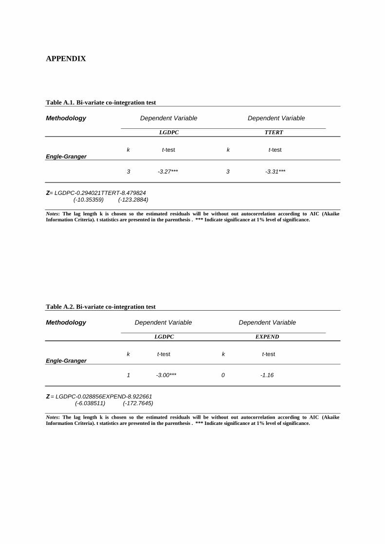
Table A.1. and Table A.217

. summarize the empirical results using the two-step Engle

Granger co-integration method The results suggest that the hypothesis of no co-integration

between the education variables and GDP growth can be rejected. To verify the results, the

Phillips –Hansen method was applied. Table. A.3. and Table A.4. summarize the results of

fully modified ordinary least squares estimator of Phillips Hansen (FMOLS).

The combined results from the previous estimation techniques suggest the existence of

a long-run relationship between human capital and economic growth.

Table A.5. and Table A.6. present the results of co-integration analysis among the two

variables using the Johansen maximum likelihood approach employing both the maximium

eigenvalue and trace statistic. The results of co-integration tests with enrolments in various

levels of education (except Primary Education), public educational expenditures and real

GDPC, indicate that there is one co-integrating vector.18

16

All the results are available from the author upon request. 17

All tables at the Appendix are referring to estimation of the GDPC and TTERT bi-variate model and the

GDPC and EXPEND bi-variate model, the results for the other estimated bi-vaiate models are not presented here

for the economy of space and are available from the author upon request. 18

The differentials in the empirical results concern the fact that Johansen- Juselius co-integration analysis is

more appropriate for the estimation of a multi-variatiate analysis and not a bi-variate.

The combined results of the co-integration analysis from the three estimation

techniques imply that there is a positive long-run relationship between human capital and

economic growth.

4.3. Error Correction Models.

Having verified that the variables are co-integrated, vector error-correction models

(VECM) can be applied. Table A.7. and Table A.8. report the findings for the endogeneity of

human capital and economic growth, based on the error correction equations from the

estimation of Engle Granger cointegration analysis.

Estimations of the parameters show, (Tertiary Education) that the error correction

term measuring the long-run disequilibrium has the right sign and is statistically significant

for the real GDP equation. This implies that the real GDPC has a tendency to restore

equilibrium and take the brunt of any shock to the system. The t-test for the error correction

term indicates, at the 1% level of significance, that real GDPC is not weakly exogenous

variable. The significance levels associated with the Wald-test of joint significance of the sum

of the lags of the explanatory variable and the error correction term provide more information

on the impact of the educational variables on economic variables and vice versa. For the real

GDPC the results imply the Granger-endogeneity of the variable.

The VECM results from the estimation of Secondary and Primary education equations

are as follows: the t-tests for the error correction terms indicate, at the 10% level of

significance that secondary education is not weakly exogenous variable and that primary

education is weakly exogenous variable.

Finally, the estimation of public educational expenditures equation indicate that,

public educational expenditures is weakly exogenous variable and that real GDPC has a

tendency to restore equilibrium and take the brunt of any shock to the system.

Next, Table A.9. and Table A.10. present the results for the endogeneity of human

capital and economic growth, based on the error correction equations from the estimation of

Phillips Hansen cointegration analysis. All the estimations for each bi-variate model (Primary,

Secondary, Tertiary education and public educational expenditures), verify the previous

results from the Engle-Granger technique, which means that the conclusions are qualitatively

the same. But, the estimations based on the error correction equations from the estimation of

Johansen and Juselius co-integration analysis give different results (Tables A.11.and A.12.).

Specifically, the main differences occurred in all bi-variate models except Tertiary education.

Finally, the stability of the coefficients was estimated using Cusum and Cusumq tests19

. The

results imply that coefficients are stable.

4.4. Summary of the estimated Granger causality results.

Table 1, summarizes the findings for the long-run, the short-run and the Granger

causality of the variables. At the second, third and fourth column of the table, all the

estimated coefficients of the independent variables are presented employing the three co-

integration methodologies20

. All the estimated coefficients are statistically significant at 1%

level of significance and have a positive sign. The combined results of all methodologies

19

Cusum and Cusumq tests are presented at the Appendix. 20

Coefficient(1) is referring to the Engle-Granger co-integration test, coefficient(2) to the Phillips-Hansen co-

integration test and finally Coefficient(3) to the Johansen and Juselius methodology.

Table 1. Summary of the results for the long-run, the short-run and the Granger causality of the variables.

Long-Run relationship Short-Run relationship

Μεθοδολογία OLS Phillips-Hansen Johansen-Juselius

Strict exogeneity Weak exogeneity Strong exogeneity Granger Causality (error correction term)

OLS P-H J-J OLS P-H J-J OLS P-H J-J

Coefficient(1) Coefficient(2) Coefficient (3)

Note: T is the time trend in the long-run relationship. ***, **, * and indicate significance at 1%, 5%, and 10% levels.

TPRIM → GDPC GDPC →TPRIM TSEC → GDPC GDPC →TSEC TTERT → GDPC GDPC → TTERT ΤTOTAL → GDPC GDPC → ΤTOTAL EXPEND → GDPC GDPC → EXPEND

0.130***(τ)

0.052***

(τ)

0.294***

0.048***

(τ)

0.029***

0.134***(τ)

0.042***

(τ)

0.288***

0.045***(τ)

0.031***

-0.091

0.524***(τ)

0.198***

0.195***(τ)

0.020***

YES

NO

YES

YES YES YES YES YES

YES

YES

YES

NO

YES

YES YES

YES

YES

YES

YES YES

---

---

---

---

YES YES

---

---

---

---

-0.12*

0.68

-0.06

0.99* -0.10***

0.21

-0.07

1.78

-0.09***

1.05

-0.12

0.76 -0.08*

0.89

-0.10***

0.21

-0.07

1.66

-0.08***

-1.41

---

--- 0.02***

0.16*** -0.11***

0.10

0.04***

0.70***

-0.08***

1.11

YES

NO

YES

NO

NO

YES

YES

NO

NO

YES

YES

NO YES

NO

NO

YES

YES

NO

NO

YES

---

---

---

---

NO YES

---

---

---

---

absence

causality

absence

causality

causality

absence

absence

causality

causality

absence

indicate that for all estimated bi-variate models there is one co-integrating vector. The

findings of the existence of a positive long-run relationship between human capital and

economic growth are in line with previous researchers such as Pereira and Aubyn (2009) for

Portugal, Babatunde and Adefabi (2005) for Nigeria and Asteriou and Agiomirgianakis

(2001), for Greece.

Next, referring to the empirical results of the short-run dynamics (Granger- causality

in the strict sense), the Wald-tests indicate that there is a relationship between Primary

education and real GDPC and that enrolment rates in all levels of education should be

considered as an endogenous variable. The combined results of all methodologies indicate

that the real GDPC depends on Tertiary education and the public expenditures on education,

while Primary education is affected by economic growth.

5. CONCLUSIONS AND POLICY IMPLICATIONS

In this paper we examined the causal relationship between education and economic

growth for Greece covering the period from 1961 to 2006, using a bi-variate approach based

on human capital theory.

Empirical results suggests that in the long-run period real GDP per capita is affected

by changes in primary, secondary, tertiary education and educational public expenditures.

The empirical results using the error-correction estimation indicate that the direction

of causality runs from Tertiary Education and public educational expenditures to real GDP

per capita and that both variables should be considered as exogenous variable. As for the

primary and secondary education, the findings reveal that causality runs through the opposite

direction, from real GDPC to the levels of education. All the estimations have shown the

existence of a uni-direction causality between human capital and economic growth in Greece.

The findings have important policy implications for Greece because of the economic

uncertainty, which affects all sectors and every aspect of human activity, including education.

Conclusions drawn from this analysis could be useful for educational policy makers to invest

in education. Specifically, there is a motivation for the government to increase the public

expenditures on education and to expand the number of students in Tertiary education, since

that cause economic growth. Further investigation for a multivariate approach is an open

issue, since there are some difficulties with the availability of the data.

Acknowledgements

The author wishes to thank Professor George Hondroyiannis for useful comments and discussion in a

previous version of this paper. The views expressed in this paper are those of the author and not those

of Harokopio University.

REFERENCES

Asteriou, D., and Agiomirgianakis G., M (2001). “Human Capital and Economic Growth: Time

Series Evidence From Greece”, Journal of Policy Modeling, 23:5, 481--489.

Ahmed, S (2009). Human Capital and Regional Growth: Α Spatial Econometric Analysis of

Pakistan, Thesis, Florence, Italy.

Ararat, O. (2007). “The Role of Education in Economic Growth in The Russian Federation and

Ukraine”, MPRA Paper 7590, University Library of Munich, Germany.

Babatunde., M. A., and Adefabi R., A. (2005). “Long Run Relationship Between Education and

Economic Growth in Nigeria: Εvidence From the Johansen‟s Cointegration Approach”,

Regional Conference on Education in West Africa: Constrains and Opportunities in Dakar,

Senegal, 1-2 Νovember 2005.

Boccanfusso, D., Savard, L. and Savy B. (2009). “Human Capital and Growth: New Evidences

from African Data”, Working Paper, No. 09-24.

Boldin, R., Morote, E., S., and McMullen M. (2008). “Higher Education and Economic Growth

in Latin American Emerging Markets” Latin American Studies, 16:18,1--17.

Bouaissa, M. (2009). “Human Capital Theory, Returns to Education and On the Job Learning:

Evidence From the Canadian Data”, Preliminary and Incomplete Version, CEA, 43rd Annual

Conference, University of Toronto, Ontario, May 29-31, 2009.

Chandra, A., and. Islamia J., M. (2010).“Does Government Expenditure on Education Promotes

Growth? An Econometric Analysis” Forthcoming in: Journal of Practicing Managers.

Dananica, D., M., and Belasku L. (2008), “The Interactive Causality Between Higher Education

and Economic Growth in Romania”, Economics of Education Review, 17:1, 361--372.

Dauda, R., O., S. (2009).“Investment in Education and Economic Growth in Nigeria: A

Cointegration Approach” 9th Global Conference on Business and Economics, University of

Cambridge, UK, October 16-17, 2009.

De Meulemeester, J., L., and. Rochat D. (1995). “A Causality Analysis of the Link Between

Higher Education and Economic Development”, Economics of Education Review, 14:4,351--

361.

EL. STAT. (2009). Survey for Employment of Labor Force, Hellinic Statistical Authority,

Athens. [In Greek].

Hondroyiannis, G., and Papapetrou E. (2002).“Demographic Transition and Economic Growth:

Εmpirical Evidence From Greece”, Journal of Population Economics, 23:15, 221--242.

Huang, F., Jin L., and Sun X. (2009). “Relationship Between Scale of Higher Education and

Economic Growth in China”, Asian Social Sciences, 5:11, 55--61.

Islam, T., S., Wadud, M., A., and Islam Q., B., T. (2007). “Relationship Between Education and

GDP Growth: Α Μultivariate Causality Analysis for Bangladesh” Economics Bulletin, 3:35, 1--

7.

Κhalifa, Y., Al.-Y. (2008). “Education Expenditure and Economic Growth: Some Empirical

Evidence from the GGC Countries”, Journal of Developing Areas, 42:1, 69--80.

Lin, T., C. (2004). “The Role of Higher Education in Economic Development: Αn Empirical

Study of Taiwan”, Journal of Asian Economics, 15, 355--371.

Loening, J., L. (2010). “Εffects of Schooling Levels on Economic Growth: Time Series

Evidence From Guatemala”, MPRA Paper, No. 25105, University Library of Munich, Germany.

Maksymenko, S., and Rabbani M (2009). “Economic Reforms, Human Capital, and Economic

Growth in India and South Korea: A Cointegration Analysis, Working Papers, No.361.,

University of Pittsburg, Department of Economics.

Matsushita, S., Siddique, A., and Giles M. (2006). “Education and Economic Growth: A Case

Study of Australia”, Economic Discussion /Working Papers, No. 06-15, The University of

Western Australia, Department of Economics.

Οdit, M., P. and Dookhan K. (2010), “The Impact of Education on Economic Growth The Case

of Mauritius”, Conference Procedings.

Papapetrou, E. (2006). “The Saving Investment Relationship in Case of Structural Change, The

Case of Greece”, Journal of Economics Studies, 33: 3 ,121--129.

Pereira, J., and Aubyn M., St (2009). “What Level of Education Matters Most For Growth?

Evidence From Portugal”, Economics of Education Review, 28:1, 67--73.

Pradhan, R., P. (2009). “Education and Economic Growth in India: Using Error Correction

Modelling”, International Journal of Finance and Economics, 25, 139--147.

Psacharopoulos, G. (1995). “The Profitability of Investment in Education: Concepts and

Methods”, The World Bank, Human Capital Development, Working Papers, No.76.

Schutt, A. (2005), “The Importance of Human Capital For The Economic Growth”, Institute of

World Economics and International Management, No. 27.

Tsamadias, C., and Prontzas P. (2011). “The Effect of Education on Economic Growth in

Greece Over the 1960-2000 Period” (forthcoming).

Wilson, A., B., and Briscoe G. (2004). “The Impact of Human Capital Growth: Α Review”,

Third Report on Vocational Training Research in Europe: Α Background Report, Reference

Series 54.

APPENDIX

Table A.1. Bi-variate co-integration test

Methodology Dependent Variable Dependent Variable

LGDPC TTERT

k t-test k t-test Engle-Granger

3 -3.27*** 3 -3.31***

Ζ= LGDPC-0.294021TTERT-8.479824 (-10.35359) (-123.2884)

Notes: The lag length k is chosen so the estimated residuals will be without out autocorrelation according to AIC (Akaike

Information Criteria). t statistics are presented in the parenthesis . *** Indicate significance at 1% level of significance.

Table A.2. Bi-variate co-integration test Methodology Dependent Variable Dependent Variable

LGDPC EXPEND

k t-test k t-test Engle-Granger

1 -3.00*** 0 -1.16

Ζ = LGDPC-0.028856EXPEND-8.922661

(-6.038511) (-172.7645)

Notes: The lag length k is chosen so the estimated residuals will be without out autocorrelation according to AIC (Akaike

Information Criteria). t statistics are presented in the parenthesis . *** Indicate significance at 1% level of significance.



LGDPC TTERT

k t-test k t-test Phillips-Hansen

3 -3.13*** 3 -3.28***

Ζ = LGDPC-0.28800TTERT-8.5190

(-7.4777) (-90.3778)

Notes: The Phillips and Hansen estimates are based on the Parzen lag window. The lag length k is chosen so the estimated residuals

will be without out autocorrelation according to AIC (Akaike Information Criteria). t statistics are presented in the parenthesis. ***

Indicate significance at 1% level of significance.



LGDPC EXPEND

k t-test k t-test Phillips-Hansen

0 -3.16*** 3 -0.67

Ζ = LGDPC-0.030765EXPEND-8.9420

(-4.9668) ( -132.1156)

Notes: The Phillips and Hansen estimates are based on the Parzen lag window. The lag length k is chosen so the estimated residuals

will be without out autocorrelation according to AIC (Akaike Information Criteria). t statistics are presented in the parenthesis. ***

Indicate significance at 1% level of significance.

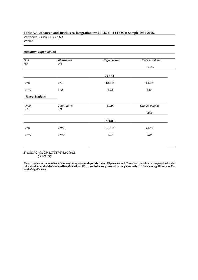
Table A.5. Johansen and Juselius co-integration test (LGDPC -TTTERT): Sample 1961-2006.

Variables: LGDPC, TTERT Var=2

Maximum Eigenvalues

Null Alternative Eigenvalue Critical values Η0 Η1 95%

TTERT

r=0 r<=1 Trace Statistic

r=1 r=2

18.53**

3.15

14.26

3.84

Null H0

Alternative Η1

Trace

Critical values

95%

TTERT

r=0 r<=1

r>=1 r>=2

21.68**

3.14

15.49

3.84

Z=LGDPC -0.198411TTERT-8.699612 (-4.58912)

Note: r indicates the number of co-integrating relationships. Maximum Eigenvalue and Trace test statistic are compared with the

critical values of the MacKinnon-Ηaug-Michelis (1999). t statistics are presented in the parenthesis. ** Indicates significance at 5%

level of significance.

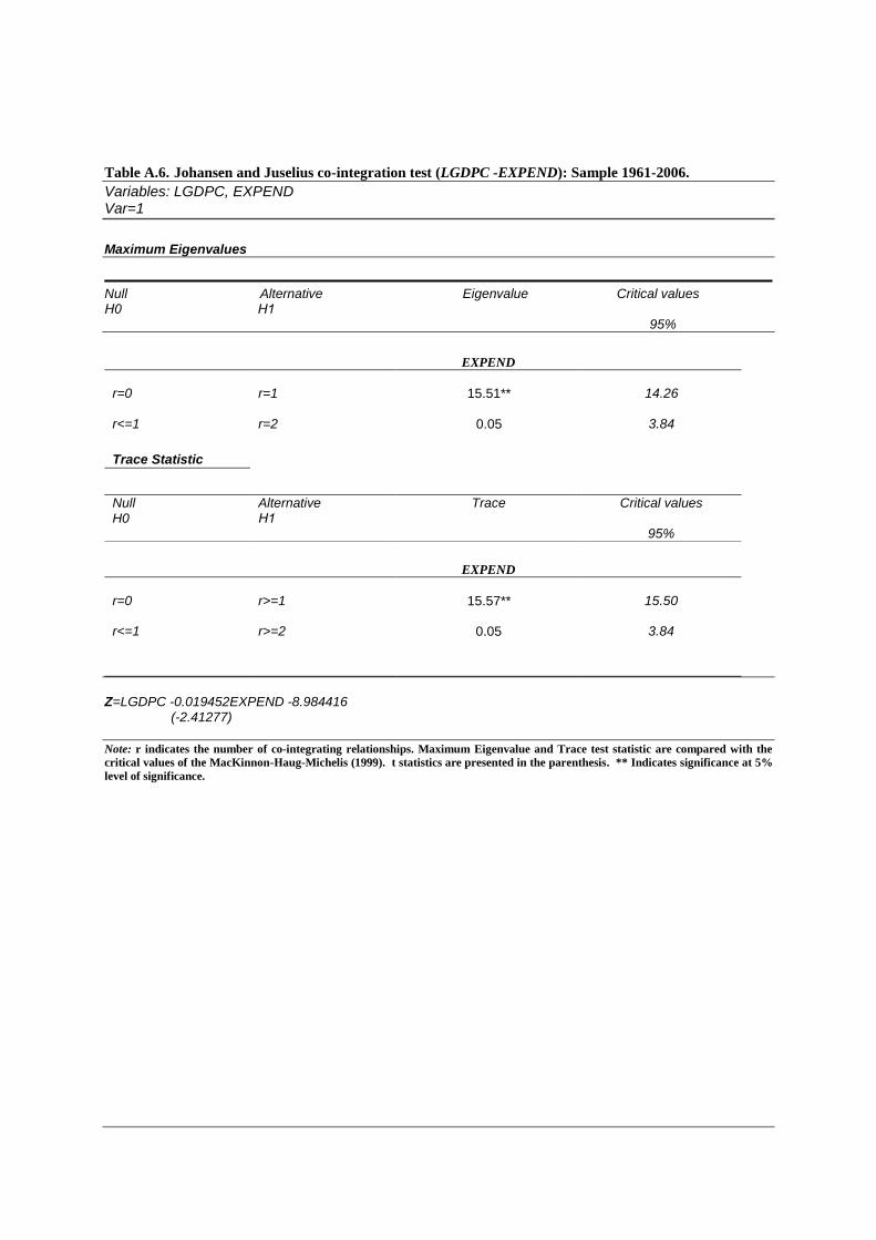
Table A.6. Johansen and Juselius co-integration test (LGDPC -EXPEND): Sample 1961-2006.

Variables: LGDPC, EXPEND Var=1

Maximum Eigenvalues

Null Alternative Eigenvalue Critical values Η0 Η1 95%

EXPEND

r=0 r<=1

Trace Statistic

r=1 r=2

15.51**

0.05

14.26

3.84

Null H0

Alternative Η1

Trace

Critical values

95%

EXPEND

r=0 r<=1

r>=1 r>=2

15.57**

0.05

15.50

3.84

Z=LGDPC -0.019452EXPEND -8.984416 (-2.41277)

Note: r indicates the number of co-integrating relationships. Maximum Eigenvalue and Trace test statistic are compared with the

critical values of the MacKinnon-Ηaug-Michelis (1999). t statistics are presented in the parenthesis. ** Indicates significance at 5%

level of significance.

Table A.7. Tests for weak and strong exogeneity of variables based on Engle-Granger Co-integration test.

EQUATIONS TESTS OF RESTRICTIONS

ΔLGDPC ΔTTERT Z=0 ΔLGDPC ΔΤTERT & ΕCT & ΕCT

ΔLGDPC - 0.02 -0.10*** - 7.12*** ΔTTERT 0.37 - 0.21 1.07 -

Note: The lagged (ECT) is derived by normalizing the cointegrating vector on LGDPC. *** Indicate significance at 1% level of

significance.

Table A.8. Tests for weak and strong exogeneity of variables based on Engle-Granger Co-integration test.


ΔLGDPC ΔEXPEND Z=0 ΔLGDPC ΔEXPEND & ΕCT & ΕCT

ΔLGDPC - 1.62 -0.09*** - 9.60*** ΔEXPEND 0.25 - 1.05 0.76 -


significance.

Table A.9. Tests for weak and strong exogeneity of variables based on Phillips-Hansen Co-integration test.


ΔLGDPC ΔTTERT Z=0 ΔLGDPC ΔTTERT & ΕCT & ΕCT

ΔLGDPC - 0.02 -0.10*** - 7.41*** ΔTTERT 0.37 - 0.21 1.02 -


significance.

Short-run Weak Joint short dynamics Exogeneity dynamics and (ΕCT) Error Correction Term



Table A.10. Tests for weak and strong exogeneity of variables based on Phillips-Hansen Co-integration

test.



ΔLGDPC - 1.41 -0.08*** - 8.45*** ΔEXPEND 1.57 - -1.41 1.06 -


significance.

Table A.11. Tests for weak and strong exogeneity of variables based on Johansen-Juselius Co-integration

test.


ΔLGDPC ΔTERT Z=0 ΔLGDPC ΔΤTERT & ΕCT & ΕCT

ΔLGDPC - 0.15 -0.10*** - 14.04*** ΔTTERT 0.18 - - 0.06 1.05 -


significance

Table A.12. Tests for weak and strong exogeneity of variables based on Johansen-Juselius Co-integration

test.



ΔLGDPC - - -0.08*** - - ΔEXPEND - - 1.11 - -


significance.




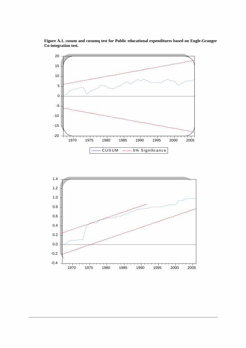
Figure A.1. cusum and cusumq test for Public educational expenditures based on Engle-Granger

Co-integration test.

-20

-15

-10

-5

0

5

10

15

20

1970 1975 1980 1985 1990 1995 2000 2005

C U S U M 5 % S i g n i f i c a n c e

C U S U M o f S q u a r e s 5 % S i g n i f i c a n c e

-0.4

-0.2

0.0

0.2

0.4

0.6

0.8

1.0

1.2

1.4

1970 1975 1980 1985 1990 1995 2000 2005

Figure A.2. cusum and cusumq test for Tertiary Education based on Engle-Granger Co-

integration test.

-0.4

-0.2

0.0

0.2

0.4

0.6

0.8

1.0

1.2

1.4

1970 1975 1980 1985 1990 1995 2000 2005


-20

-15

-10

-5

0

5

10

15

20

1970 1975 1980 1985 1990 1995 2000 2005


Figure A.3. cusum and cusumq test for Public educational expenditures based on Phillips-

Hansen Co-integration test.

α 9.8. Έλεγχος ιζοδυναμίας ζυνηελεζηών ηου διανυζμαηικού υποδείγμαηος διό


-0.4

-0.2

0.0

0.2

0.4

0.6

0.8

1.0

1.2

1.4

1970 1975 1980 1985 1990 1995 2000 2005


-20

-15

-10

-5

0

5

10

15

20

1970 1975 1980 1985 1990 1995 2000 2005

Figure A.4. cusum and cusumq test for Tertiary Education based on Phillips- Hansen Co-

integration test.

-20

-15

-10

-5

0

5

10

15

20

1970 1975 1980 1985 1990 1995 2000 2005


-0.4

-0.2

0.0

0.2

0.4

0.6

0.8

1.0

1.2

1.4

1970 1975 1980 1985 1990 1995 2000 2005


Figure A.5. cusum and cusumq test for Public educational expenditures based on Johansen-

Juselius Co-integration test.

-20

-15

-10

-5

0

5

10

15

20

65 70 75 80 85 90 95 00 05


-0.4

-0.2

0.0

0.2

0.4

0.6

0.8

1.0

1.2

1.4

65 70 75 80 85 90 95 00 05


Figure A.6. cusum and cusumq test for Tertiary Education based on Johansen-Juselius Co-

integration test.

-0.4

-0.2

0.0

0.2

0.4

0.6

0.8

1.0

1.2

1.4

1970 1975 1980 1985 1990 1995 2000 2005



-20

-15

-10

-5

0

5

10

15

20

1970 1975 1980 1985 1990 1995 2000 2005

Documents

Relationship Between Education and GDP Growth: A Bi ... pdf/Events/2011-5th...Relationship Between Education and GDP Growth: A Bi-variate Causality Analysis for Greece M. Solaki1*