Embed Size (px)
Citation preview

Relationship between fine-mode AOD and
precipitation on seasonal and interannual time scales
By HWAYOUNG JEOUNG1, CHUL E. CHUNG1*, TWAN VAN NOIJE2 and
TOSHIHIKO TAKEMURA3, 1School of Environmental Science and Engineering, Gwangju Institute
of Science and Technology, Gwangju 500-712, Korea; 2Royal Netherlands Meteorological Institute, De Bilt,
The Netherlands; 3Research Institute for Applied Mechanics, Kyushu University, Fukuoka, Japan
(Manuscript received 10 October 2013; in final form 11 December 2013)
ABSTRACT
On seasonal and interannual time scales, weather is highly influential in aerosol variability. In this study, we
investigate the relationship between fine-mode AOD (fAOD) and precipitation on these scales, in order to
unravel the effect of wet weather on aerosol amount. We find with integrated satellite and ground observations
that biomass burning related fAOD has a relatively greater seasonal variation than fossil fuel combustion
related fAOD. It is also found that wet weather reduces biomass burning fAOD and increases fossil fuel
combustion fAOD. Aerosol simulation models forced by reanalyses consistently simulate the biomass burning
fAOD reduced during wet weather but only in the tropics and furthermore do not consistently increase fossil
fuel combustion fAOD during wet conditions. The identified relationship between fAOD and precipitation in
observations allows for seasonal predictability of fAOD, since average precipitation can be predicted a few to
several months in advance due to the well-established predictability of El Nino-Southern Oscillation (ENSO).
We reveal ENSO-covariant fAOD using a rotated component principal analysis of combined interannual
variation of sea surface temperature, precipitation and fAOD. During the warm phase of ENSO, we find that
fAOD increases over Indonesia and the eastern coastal area of China, and decreases over South Asia, the
Amazon and the continental parts of China.
Keywords: aerosol, AOD, aerosol simulation, weather, meteorology, prediction
1. Introduction
The amount, distribution and composition of aerosols in
the atmosphere are controlled by emission and weather.
Weather affects aerosols by various meteorological vari-
ables such as temperature, humidity, cloud cover, precipita-
tion, wind and boundary layer stability. Jacob and Winner
(2009) summarised how each meteorological variable influ-
ences aerosol dry mass in aerosol simulations. For example,
higher humidity causes greater aerosol mass, while pre-
cipitation decreases aerosol mass. Tai et al. (2010), by
analysing PM2.5 observations, showed that humidity,
with other meteorological variables held fixed, is positi-
vely correlated with sulphate and nitrate, but negatively
with organic aerosol (OA) and black carbon (BC). Note
that meteorological variables are consistent with one
another dynamically, thermodynamically and physically.
For instance, precipitation tends to be accompanied by high
moisture and larger cloud coverage.
On multidecadal to centurial time scales, anthropo-
genic aerosol emission can change several-fold (Lamarque
et al., 2010), and so emission can be the driving factor in
determining aerosols. On the other hand, on seasonal and
interannual (2�4 years) scales, weather is expected to be a
relatively more important factor in determining the varia-
bility of aerosols. On these time scales, aerosol emissions
resulting from fossil fuel combustion fluctuate notice-
ably but much less than several-fold in most places. For
instance, SO2 emission in China is estimated to vary 20%
seasonally and 30�40% interannually (Lu et al., 2011).
SO2 emission is a good proxy for fossil fuel combustion.
Emission of biomass burning aerosols is estimated to vary
noticeably too (Van der Werf et al., 2006; Cohen and
Wang, 2013). For instance, over open biomass burning
regions in Africa, the emission was estimated to change
from year-to-year by about 15�20% (Van der Werf et al.,
2006; Cohen and Wang, 2013). This fluctuation of biomass*Corresponding author.
email: [email protected]
Tellus B 2014. # 2014 H. Jeoung et al. This is an Open Access article distributed under the terms of the Creative Commons CC-BY 4.0 License (http://
creativecommons.org/licenses/by/4.0/), allowing third parties to copy and redistribute the material in any medium or format and to remix, transform, and build
upon the material for any purpose, even commercially, provided the original work is properly cited and states its license.
1
Citation: Tellus B 2014, 66, 23037, http://dx.doi.org/10.3402/tellusb.v66.23037
P U B L I S H E D B Y T H E I N T E R N A T I O N A L M E T E O R O L O G I C A L I N S T I T U T E I N S T O C K H O L M
SERIES BCHEMICALAND PHYSICALMETEOROLOGY
(page number not for citation purpose)

burning aerosol emission appears to be largely weather
related. Murdiyarso and Adiningsih (2007) explain that dry
weather conditions are more suitable for biomass burning.
Weather can also account, at least partially, for seasonal or
interannual fluctuations of fossil fuel combustion though
the extent is not known. Overall, it is safe to say that
weather is highly influential in aerosol variability on
seasonal and interannual scales. We also note that volcanic
eruptions can disturb the aerosol amount and character-
istics greatly for up to 2 years, and volcanic eruptions are
considered weather independent.
In the present study, we attempt to unravel the relation-
ships between aerosol and precipitation on seasonal and
interannual time scales. Correlations between PM concen-
tration and meteorological variables have been investigated
in the past (Koch et al., 2003; Wise and Comrie, 2005;
Tai et al., 2010). When precipitation occurs, it scavenges
aerosols and removes them from the atmosphere. The
accompanying cloudiness decreases the photochemical oxi-
dation of SO2 and decreases sulphate, while in-cloud pro-
duction increases sulphate (Jacob and Winner, 2009). The
accompanying moisture enlarges sulphate aerosol by water
uptake (Hess et al., 1998). The wet condition associated
with precipitation would suppress open biomass burning.
We include all these effects by seeking a simple correlation
or covariance of aerosol and precipitation. A unique aspect
of our study is that we seek to explore seasonal (a few to
several months) predictability of aerosols. Precipitation
has short-term climate predictability given the influence of
El Nino-Southern Oscillation (ENSO). ENSO is being
successfully predicted several months in advance (e.g. US
Climate Prediction Center). Ropelewski and Halpert (1987)
demonstrated that during El Nino phase precipitation
decreases over Indonesia and Australia while precipita-
tion is enhanced over the southern portion of the US.
Precipitation predictability can lead to aerosol predic-
tability, once a precipitation�aerosol relationship is estab-
lished. Studies addressing ENSO impacts on aerosols
exist; for instance, Wu et al. (2013) revealed a biennial
component of aerosol variability over the Maritime Con-
tinent (58S�58N, 95�1358E) and the western North Pacific
Ocean. The novelty of the current study is to analyse the
fine-mode aerosol optical depth (fAOD) in relation to
ENSO.
Aerosols have different sizes, and typically follow a
bimodal structure in terms of fine mode and coarse mode
(Kim et al., 2007; Viskari et al., 2012). Fine-mode aerosols
usually have submicron sizes in diameter and consist
largely of BC, OA, sulphate, or nitrate. These small par-
ticles are mostly anthropogenic. Schwartz and Neas (2000)
reported that small particles are more harmful for human
respiratory health than coarse-sized particles. One can use
PM1.0 measurements to study fine-mode particles. Here,
we focus on fAOD because optical depth carries additional
useful information such as visibility and the impact on the
radiation balance. We analyse fAOD also because satellite
measurements give a nearly global coverage. Global AOD
(aerosol optical depth) can be obtained from the Moderate
Resolution Imaging Spectroradiometer (MODIS) and
Multi-angle Imaging Spectroradiometer (MISR) satellite
sensors. The fine-mode fraction (FMF) of total AOD is
also retrieved and its retrieval algorithm depends heavily on
the spectral variation of AOD (Remer et al., 2005). Due to
the uncertainties in the spectral variation of land surface
albedo, satellite-derived FMF is not reliable over land. Lee
and Chung (2013) on the other hand constructed more
reliable FMF over the globe by nudging satellite data
towards Aerosol Robotic NETwork (AERONET) data.
We will analyse fAOD data from Lee and Chung (2013).
For comparison, global aerosol simulations will also be
analysed.
Aerosols also affect weather and climate. Aerosols scat-
ter and absorb solar radiation in the atmosphere (the so-
called direct effect). Big particles such as dust and sea salt
also absorb longwave radiation. The absorption of radia-
tion increases air temperature. The absorption and scatter-
ing of radiation reduces the radiation reaching the surface
and will likely decrease evaporation and precipitation
(Ramanathan et al., 2001). Some of the aerosols can
absorb sunlight efficiently and heat the atmosphere. This
heating can evaporate cloud condensate and reduce cloud
amount (the so-called semi-direct effect). Some aerosols
act as cloud condensation nuclei (CCN), thus affecting
cloud albedo and lifetime (the so-called indirect effect). By
seeking the relationships between aerosol and precipitation,
we do not separate the effect of meteorology on aerosol
from that of aerosol on weather. Such separation is very
important to validate models but irrelevant to empirical
prediction of aerosol based on correlation between pre-
cipitation and aerosol.
We organise the paper in six sections. Section 2 describes
the observations and model simulations. In section 3,
we discuss the climatology and variance of fAOD. The
correlation between precipitation and fAOD is discussed in
section 4. In section 5, we describe ENSO-covariant fAOD.
Conclusion and discussion follow in section 6.
2. Data
In this section, we describe the observations and model
simulations employed for the analysis here. All the data
(including simulation results) are monthly means and
processed onto the T42 spatial resolution before statistical
analyses. The T42 resolution is approximately 2.88�2.88.
2 H. JEOUNG ET AL.

2.1. Observation
AOD and fAOD are obtained by the approach described
in Lee and Chung (2013), who integrated monthly mean
MODIS,MISR andAERONETdata. They integrated these
data by nudging the combined satellite data towards the
AERONET data so as to construct reliable AOD and fAOD
fields over the globe. We refer to this integrated data as
MODIS�MISR�AERONET data here. As Lee and
Chung (2013) explain, the data integration consists of the
following steps: (1)MODIS andMISRdata are combined to
reduce the data gaps and improve the accuracy; (2) the
remaining gaps are filled by the Georgia Tech/Goddard
Global Ozone Chemistry Aerosol Radiation and Transport
(GOCART) simulation (Chin et al., 2002); and (3) the com-
bined MODIS�MISR�GOCART data are nudged to-
wards the AERONET data as though the MODIS�MISR�GOCART data were an interpolation tool. The
GOCART simulations in the MODIS�MISR�GOCART
data are predominantly confined to the polar regions.
Lee and Chung (2013) also validated the MODIS�MISR�AERONET fAOD and found that this fAOD
is closer to AERONET fAOD accuracy than MODIS
or MISR fAOD accuracy. The MODIS�MISR�AERONET AOD and fAOD data span from 2001 to
2010. To facilitate the data comparison, we also analyse
2001�2010 MODIS AOD, which has gaps.
Precipitation data is taken from the Global Precipitation
Climatology Project (GPCP) (Adler et al., 2003). The sea
surface temperature (SST) data is from theNational Oceanic
and Atmospheric Administration (NOAA) Optimum Inter-
polation (OISST; Version 2) (Reynolds et al., 2002).
2.2. Global aerosol simulation
We use AOD and fAOD simulations from global aerosol
models to be compared with the observations. We analyse
the output from two models: the Spectral Radiation-
Transport Model for Aerosol Species (SPRINTARS),
and the Tracer Model 5 (TM5). In particular, we use the
output from the AeroCom (Aerosol Comparisons between
Observations and Models) Phase II (Schulz et al., 2009)
hindcast experiment, in which the models used time-
varying IPCC emissions (Lamarque et al., 2013) and
reanalysis meteorology.
TM5 (Huijnen et al., 2010; Aan de Brugh et al., 2011)
was driven by meteorological fields from the ERA-Interim
reanalysis (Dee et al., 2011) from 2000 to 2009. The pre-
cipitation data which forced the model was also from the
ERA-Interim reanalysis. As Fig. 1 shows, this precipitation
data is extremely similar to the GPCP precipitation data.
TM5 uses the modal microphysics scheme M7 (Vignati
et al., 2004) to represent sulphate, BC, organic carbon, sea
salt, dust and aerosol water, together with a thermody-
namic model to describe the equilibrium of the secondary
inorganics (sulphate, ammonium and nitrate). In M7, five
out of the seven modes are internally mixed. The aerosol
optical properties (such as AOD) are based on the Mie
theory. For internally mixed aerosols, the model applies
a volume-weighted mixing of refractive indices within each
mode, using the well-known Bruggeman and Maxwell
Garnett mixing rules (Garnett, 1904; Bruggeman, 1935),
where BC and dust are treated as inclusions. The total
AOD is computed by summing up the contributions from
the different modes. fAOD consists of BC, OA, sulphate,
nitrate and the fine-mode contributions from sea salt and
dust. AOD results from the same model setup were
analysed by Von Hardenberg et al. (2012).
TM5 differentiates between clear-sky and all-sky relative
humidity. In calculating AOD, the clear-sky humidity is
used while aerosol mass in all-sky conditions is used. Thus,
the TM5 AOD can be considered clear-sky AOD overall.
In comparison, satellite-derived AODs are based on clear-
sky pixels while AOD in AERONET is retrieved as long as
there is a gap in cloud between the sun and the instrument.
In view of this, we note that TM5 AOD and MODIS�MISR�AERONET AOD have slightly different treat-
ments of cloud effects.
Anthropogenic and biomass burning emissions were
prescribed based on a combination of the Atmospheric
Chemistry and Climate Model Intercomparison Project
(ACCMIP) dataset for the year 2000 and the RCP4.5 sce-
nario data for the years 2005 and 2010 (Lamarque et al.,
2013), using a linear interpolation for the intermediate years.
Thus, the interannual variation of the anthropogenic and
biomass burning emission applied in themodel is unrealistic,
especially in view of no consideration of interannually-
varying weather on biomass burning emission. The seasonal
variation of anthropogenic emission is not realistic either, in
that the ACCMIP emissions only included a seasonal
variation from shipping and aircraft and ignored the
seasonal variation in the other anthropogenic sectors
(Lamarque et al., 2010). We find that SO2 emission in
eastern China in this emission dataset varies by less than 1%
seasonally, while, as stated in section 1, SO2 emission in
China is estimated to fluctuate by 20%seasonally byLu et al.
(2011). On the other hand, the ACCMIP dataset does
include the full seasonal variation of biomass burning
emission. Over Africa, BC emission in the ACCMIP data
is estimated to change about three-fold from the lowest
emission month to the highest emission month. In compar-
ison, the optimised BC emission estimated by Cohen and
Wang (2013) gives a slightly larger seasonal fluctuation. We
also note that the BC emission in the ACCMIP dataset likely
has low biases; for instance, the global BC emission in the
year 2000 is about 7.6 Tg while Cohen and Wang (2013)
FINE-MODE AOD AND PRECIPITATION ON SEASONAL AND INTERANNUAL TIME SCALES 3

estimate the global emission to be between 14.6 and 22.2 Tg/
yr. Cohen and Wang (2013) used aerosol observations such
as AERONET data to derive the estimates while Lamarque
et al.’s (2010) employed a bottom-up approach. For mineral
dust, the year-2000 dataset provided to AeroCom phase I as
described in Dentener et al. (2006) was applied. Sea salt and
dimethylsulfate (DMS) emissions were calculated online and
were thus allowed to change depending on the meteorology.
The SPRINTARS is a global aerosol model (Takemura
et al., 2000, 2002, 2005, 2009) coupled with a general
circulation model MIROC (Watanabe et al., 2010), which
includes the aerosol�radiation and aerosol�cloud interac-
tions. The simulation in this study is nudged by temperature
and horizontal wind from the National Centers for Atmo-
spheric Prediction (NCEP)/National Center for Atmo-
spheric Research (NCAR) reanalyses (Kalnay et al., 1996)
from 1980 to 2008. In this model, aerosols are externally
mixed except for BC and OA, which are mixed internally
using a volume-weighted mean value for the refractive
index. The total AOD is the sum of the AODs from
Fig. 1. 2001�2008 average fAOD (fine-mode AOD) and precipitation for the DJF (December, January, February) season.
4 H. JEOUNG ET AL.

individual aerosol species and the AOD of internally mixed
BC�OA aerosol. fAOD consists of BC, OA, sulphate and
the fine-mode contributions from sea salt and dust. The
AOD computed in this model excludes the times and
locations where the total cloud fraction is greater than
0.2, thus representing clear-sky AOD. In this regard, the
treatment of cloud effect is similar to that of the observed
AOD by satellite or AERONET.
Anthropogenic and biomass burning emissions are the
same as in TM5. Mineral dust emission and sea salt are
calculated online. The dust emissions in the SPRINTARS
model are much greater than those in TM5 in Asia,
whereas these two models have comparable dust emissions
over the Sahara. Conversely, the sea salt emission in the
SPRINTARS model is much less than that in TM5.
3. Climatology and interannual variation
Figures 1 and 2 display 2001�2008 average fAOD and
precipitation for DJF (December, January, February) and
Fig. 2. Same as Fig. 1 except for the JJA (June, July, August) season.
FINE-MODE AOD AND PRECIPITATION ON SEASONAL AND INTERANNUAL TIME SCALES 5

JJA (June, July, August). Among the most conspicuous
features are low fAOD biases in simulations relative
to the observation. SPRINTARS tends to have lower
fAOD than the observation, and TM5 gives even smaller
values. In a global and annual average, the MODIS�MISR�AERONET fAOD is 0.09, SPRINTARS 0.06,
and TM5 0.035. Thus, the observed fAOD is 1.5 times
as high as SPRINTARS fAOD and 2.6 times as high as
TM5 fAOD. Simulation biases are similar for the total
AOD; the MODIS�MISR�AERONET AOD is 0.161,
SPRINTARS 0.089, and TM5 0.073. These low biases
possibly imply that these two models have a too-fast
removal of aerosols by wet deposition. It is also possible
that the emission or the formation of certain aerosol types
is underestimated. For example, as discussed in section 2,
BC emission in the models is likely underestimated, given
the observationally-constrained estimate by Cohen and
Wang (2013). Another potential source of the model defi-
ciencies is a lack of urban-scale processing in the models.
Cohen et al. (2011) demonstrated that ignoring urban
processing increases the global average AOD significantly.
The fact that the models under-simulate AOD means that
ignoring urban processing is more than offset by the factors
contributing to low biases.
Another salient feature in Figs. 1 and 2 is that areas with
substantial fAOD tend not to overlap with those with
substantial precipitation. For instance, the biomass burn-
ing aerosols in Africa are located just north of the rainfall
belt in the DJF season and south of the rainfall zone in
the JJA season. The tendency for biomass burning to
occur away from wet area is clearly evident in both
the observation and model simulations. In contrast, the
wet-area-avoiding tendency is not very clear over India and
China, where fossil fuel combustion is a very important
source of aerosol. In summer, the monsoon rainfall occurs
over India but SPRINTARS simulates larger fAOD in
summer than in winter over this region while the observa-
tion indicates otherwise. We will discuss the relationship
between fAOD and precipitation in detail in the next
section.
Temporal variations of fAOD can be split into the
climatological seasonal variation and the deviations from
the climatological seasonal variation. The latter consists
largely of interannual variation and includes intraseasonal
variability. For brevity, we refer to this latter as interannual
variation in this study. Focusing on the climatological
seasonal variation first, as the models under-simulate
fAOD and AOD, the climatological seasonal variation
for simulated AOD and fAOD is also suppressed. The
seasonal variation relative to the annual mean how-
ever, as shown in Table 1, is not underrepresented in the
models.
The spatial pattern of the climatological seasonal varia-
tion, as displayed in Fig. 3, gives additional insights. The
feature that is of particular interest is the relative strength
of the biomass burning aerosol variation to the fossil
fuel combustion aerosol variation. We assess the relative
strength by comparing the relative standard deviation (SD)
of fAOD over eastern China (which represents fossil fuel
combustion) to that over the Amazon and the open bio-
mass burning areas of Africa (which together represent
tropical biomass burning areas). In the observations, bio-
mass burning fAOD has a much greater seasonal variation
than fossil fuel combustion fAOD (Fig. 3b). The greater
seasonal variation in biomass burning aerosol might be due
partly to a greater dependence of biomass burning emission
on local weather conditions. The SPRINTARS model, on
the other hand, shows relatively strong seasonal variation
Table 1. Global average of SD (standard deviation)
2001�2008 average seasonal variation RSD (%) Interannual variation RSD (%)
AOD MODIS alone 30.4 23.8
MODIS�MISR�AERONET 26.3 30.0
SPRINTARS 32.9 32.6
TM5 23.4 15.4
fAOD MODIS�MISR�AERONET 34.3 37.1
SPRINTARS 38.7 37.3
TM5 32.7 17.2
Precipitation GPCP precipitation 46.9 49.0
SPRINTARS precipitation 43.8 74.7
TM5 precipitation 43.2 33.8
Note that the MODIS�MISR�AERONET data are the standard observation we use here and is from Lee and Chung (2013).
To compute interannual variation SD, we use the 2001�2010 period for detrended MODIS, MISR, AERONET and GPCP data, the
1980�2008 period for detrended SPRINTARS data, and the 2000�2009 period for detrended TM5 data. In computing the global average
SD, the data corresponding to the MODIS AOD gaps are removed. Instead of showing SD itself, we show the normalised values in
percentage by dividing SD by mean, which is referred to as RSD (relative SD).
6 H. JEOUNG ET AL.

over eastern China compared to the observation (Fig. 3b
vs. 3d) and compared to the seasonal variation in the
tropical biomass burning areas (Fig. 3d). The inconsistency
between the observation and the SPRINTARS might seem
counter-intuitive, in that the anthropogenic emission used
by the models under-represents the seasonal variation. Lu
et al. (2011) showed that SO2 and carbonaceous aerosol
emission in China is lowest in summer and highest in
winter. The MODIS�MISR�AERONET fAOD is lar-
gest in summer in this region. Thus, the observation
indicates that the growth of fAOD by moisture, photo-
chemistry, etc. is sufficient to more than overcome lower
emission in summer. In the models where the anthropo-
genic emission is not significantly lower in summer, the
seasonal variation might be artificially amplified over
eastern China. For TM5, however, while one might expect
Fig. 3. RSD (Relative standard deviation) of climatological (2001�2008) seasonal variation.
FINE-MODE AOD AND PRECIPITATION ON SEASONAL AND INTERANNUAL TIME SCALES 7

to see such an artificial amplification, this model shows a
weak seasonal variation in eastern China (Fig. 3f).
In a global average, the climatological seasonal variation
is slightly weaker than the interannual variation in the
standard AOD and fAOD observations (see Table 1). It is
possible that the interannual variation is stronger than
the seasonal variation because this particular observation
(which combines MODIS, MISR and AERONET data)
includes the AERONET data. AERONET data has an
uneven coverage in time, and this uneven coverage can
amplify the interannual variation component. Thus, we
re-calculated the variability using the MODIS AOD and
found that the climatological seasonal variation is slightly
stronger than the interannual variation (Table 1). On the
other hand, TM5 has most of the variability coming from
the climatological seasonal variation. This is expected,
because the interannual variation of the emission in the
model is suppressed. Despite using the same anthropo-
genic and biomass burning emissions, SPRINTARS is very
close to the observation in terms of the ratio of the clima-
tological seasonal variation to the interannual variation.
The difference between TM5 and SPRINTARS might be
due partly to the fact that the precipitation used in TM5
also has weak interannual variation while the precipita-
tion in SPRINTARS has very strong interannual variation
(Table 1). It would be interesting to see whether the models
can reproduce the observed variability partition between
the climatological seasonal variation and the interannual
variation with the same GPCP precipitation forcing.
The spatial pattern of the interannual variation is
shown in Fig. 4. The observed fAOD interannual variation
(Fig. 4b) has quite a different spatial pattern than the
observed fAOD seasonal variation (Fig. 3b) does. Large
interannual variation is found over the Amazon, Indonesia,
Australia, Canada and some parts of remote oceans
(Fig. 4b). The spatial pattern differences between the
observation (Fig. 4b) and the simulations (Fig. 4d and 4f)
are also very substantial. Figure 4 also reveals that the
tendency for TM5 to have weak interannual variation is
everywhere (Fig. 4f vs. 4d).
4. Relationship between fAOD and precipitation
Figures 1 and 2 imply that precipitation and fAOD are
negatively correlated at least over tropical biomass burn-
ing areas. In this section, we investigate the correlation
between precipitation and fAOD. The correlation arises
from the climatological seasonal variation as well as inter-
annual variation. Here, we compute the correlation due
to the climatological seasonal variation and that due to
interannual variation separately and refer to the latter as
interannual correlation for brevity. The correlation due to
the climatological seasonal variation is simply referred to as
seasonal correlation. Interannual correlation is computed
after detrending the data. Please note that our use of
monthly mean clear-sky fAOD and monthly mean pre-
cipitation means that the obtained correlation does not
describe an instantaneous relationship between fAOD and
precipitation.
Figure 5 shows the seasonal correlation for both the
observation and the models. The correlation is mostly
negative over tropical biomass burning regions such as
Indonesia, the Amazon and Central Africa. This feature is
as expected. On the contrary, the correlation over Canada,
the central part of the US and the eastern part of Siberia is
positive, particularly in the models. Out of these regions,
the ratio of SO2 emission to BC emission imposed in the
models is low in Canada and the eastern part of Siberia.
The ratio over there is higher than over the open biomass
burning regions in Africa but is comparable to that over
Indonesia, which indicates that biomass burning is prob-
ably the leading aerosol source in Canada and the eastern
part of Siberia. Thus, the positive correlation in these
regions is a puzzle.
Figure 6 is shown to further understanding the correla-
tion contrast between the tropical biomass burning areas
and the high-latitude biomass burning areas. While fAOD
seasonal variation is in antiphase with precipitation seaso-
nal variation in Africa (Fig. 6a and 6e), the fAODmaximum
in Canada occurs in summer when precipitation is neither
maximum nor minimum (Fig. 6b and 6f). Figure 6 also shows
the seasonal variation using AERONET data alone in order
to test the robustness of MODIS�MISR�AERONET
data seasonal variation. Both the AERONET data alone
and the MODIS�MISR�AERONET data show the
maximum fAOD in summer (Fig. 6b). Because the relation-
ship between fAOD and precipitation over Canada is
neither in phase nor in antiphase, we propose that the
positive seasonal correlation over the high-latitude biomass
burning areas is coincidental. We suspect that precipitation
is a minor factor in controlling the fAOD over the high-
latitude biomass burning areas and perhaps a greater factor
is temperature. Boreal forest fires generally take place in
the season when temperature is higher. In the tropics,
conversely, air is always warm and thus temperature is
unlikely a limiting factor. Please note that additional runs
and analyses would be needed to pin down the cause for
the correlation contrast, however such additional work is
beyond the scope of the present study.
China is dominated by fossil fuel combustion aerosols
especially in its eastern part (Chen et al., 2013). In addition,
the amount of aerosol is very significant in this region
which also receives a large amount of precipitation (Figs. 1
and 2). Eastern China is, in our view, a showcase for the
effect of wet weather on fossil fuel combustion aerosols.
The observed fAOD (Fig. 5b) shows a strongly positive
8 H. JEOUNG ET AL.

seasonal correlation in the eastern part of China. This is at
least in part because fossil fuel combustion AOD growth
(especially sulphate AOD growth) by moisture overwhelms
the precipitation scavenging effect. Figure 7 shows that
MODIS�MISR�AERONET fAOD and AERONET-
alone fAOD are both largest in summer, when precipitation
is the maximum. In terms of seasonal correlation, the
simulated fAOD (Fig. 5d and 5f) agrees with the observa-
tion in the northeastern part of China but not in the
southeastern part. The difference between the observa-
tion and the models in the southeastern part of China is
a puzzle and would require additional model experiments
for better understanding. Figure 7a demonstrates that the
SPRINTARS simulates largest fAOD in spring. The fact
that fAOD is neither in phase nor in antiphase with
precipitation is evidence of little influence by precipitation
Fig. 4. RSD of interannual variation. See Table 1 for the period used for each dataset.
FINE-MODE AOD AND PRECIPITATION ON SEASONAL AND INTERANNUAL TIME SCALES 9

in SPRINTARS. In this regard, the negative correlation
in the southeastern part of China (Fig. 5d) is not a robust
feature.
India has a good mixture of fossil fuel combustion
aerosols and biomass burning aerosols (Gustafsson et al.,
2009). In this country, a significant fraction of biomass
burning is estimated to be biofuel combustion (Bond et al.,
2004), which may not depend so much on weather. In
India, we see large correlation differences between AOD
and fAOD, and between the observation and the models
(Fig. 5). As Fig. 7 demonstrates, the observed fAOD is
largest in winter, when precipitation is smallest. In con-
trast, TM5 shows almost season-independent fAOD, while
SPRINTARS simulates largest fAOD in summer. One
possible explanation for the disagreement between the
models and the observation is that BC emission in the
Fig. 5. Seasonal correlation between AOD (or fAOD) and precipitation. Correlation is computed using the 2001�2008climatological seasonal variation. For consistency, precipitation used for SPRINTARS (or TM5) is used with SPRINTARS (or TM5)
AOD. Regions with low AOD (or fAOD) or precipitation variance are masked out. The mask-out threshold values are: 1e-04
(MODIS�MISR�AERONET AOD), 1e-05 (SPRINTARS AOD), 1e-08 (TM5 AOD), 1e-04 (MODIS�MISR�AERONET fAOD),
1e-05 (SPRINTARS fAOD), 1e-06 (TM5 fAOD) and 0.05 (mm/day) (precipitation).
10 H. JEOUNG ET AL.

models is significantly underestimated in India in view
of Menon et al.’s (2010) work. BC is not hydrophilic and
so BC AOD will not grow by moisture unless coated by
hydrophilic material. Furthermore, BC emission, which
is more related to biomass burning than to fossil fuel
combustion compared to SO2 emission, is likely particu-
larly strong in dry conditions, as demonstrated by Lu et al.
(2011). Thus, it is quite possible that the observation shows
a negative correlation because biomass burning aerosols
dominate over India in reality while underrepresented BC
emission in the models generates a relatively larger amount
of sulphate and thus leads to the maximum fAOD in a
moist season or seasonal independent fAOD.
The interannual variation correlation is shown in Fig. 8.
The aforementioned positive seasonal correlation over
the high-latitude biomass burning areas does not appear
in the observed interannual variations. As shown in Fig. 8b
and 8c, the correlation is more often negative than positive
over these regions. Correlation with MODIS�MISR�AERONET data on interannual time scales may not be
robust because AERONET data coverage changes in time.
To be sure, we re-calculated the interannual correlation
using MODIS AOD (Fig. 8a), which is overall consis-
tent with the interannual correlation with MODIS�MISR�AERONET AOD. Thus, on interannual time
scales, the high-latitude biomass burning aerosols also
show negative correlation with precipitation. This negative
correlation is statistically significant over many parts of
the high-latitude biomass burning region. Thus, we con-
clude that wet conditions reduce biomass burning AOD
over the globe. In contrast with the observations, the
models simulate still (though less strong) positive inter-
annual correlations over the high-latitude biomass burning
regions. This might be because the interannual variation of
emission is suppressed in the models. Additional experi-
ments are needed to better understand the exact causes.
Fig. 6. 2001�2008 climatological seasonal variation of fAOD, AOD and precipitation averaged over the African open biomass burning
region (defined here as 158W�508E & 25S8�208N) and Canada (1458�508W & 408�808N).
FINE-MODE AOD AND PRECIPITATION ON SEASONAL AND INTERANNUAL TIME SCALES 11

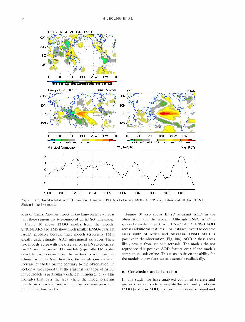
5. ENSO-covariant fAOD
To extract recurrent modes of interannual variation, such
as ENSO-covariant pattern, a rotated principal component
analysis (RPCA) using the VARIMAX criterion (Horel
and Wallace, 1981) has been commonly applied (Nigam
et al., 2000; Rogers and McHugh, 2002). At Climate
Prediction Center of the US, an RPCA is routinely applied
to monitor important large-scale variability modes such
as North Atlantic Oscillation (NAO) and Pacific/North
American (PNA) variability. In particular, a combined
RPCA technique extracts recurrent patterns of combined
variability by simultaneously analysing the structure of auto-
covariance and cross-covariance matrices. The efficacy
of this method in extracting the truly-coupled variability
modes increases with the number of variables in the
combination (Nigam and Shen, 1993). In view of this, we
conduct an RPCA of combined interannual variation of
SST, precipitation and fAOD from 2001 to 2010, from
2000 to 2008 and from 2000 to 2009 for the observation,
SPRINTARS and TM5, respectively. In conducting the
RPCA, 10 loading vectors are rotated.
Here, we describe the first mode which corresponds
to ENSO mode, as shown in Figs. 9 and 10. To test the
robustness of ENSO mode in the RPCA, we also con-
ducted linear regression with the Nino3.4 index (which is
defined as the SST anomalies averaged over the Nino3.4
region). ENSO mode obtained from the linear regression is
quite similar to ENSO mode in the RPCA, which points
out the robustness of ENSO mode obtained from the
RPCA. As Fig. 9 shows, the positive phase (i.e. warm
phase) of ENSO mode is associated with positive SST
anomalies in the eastern/central equatorial Pacific, and
negative SST anomalies in the central extratropical Pacific.
The associated precipitation anomalies are suppres-
sion over Indonesia, South Asia, Southeast Asia and
northern South America, and enhancement over the central
equatorial Pacific and the central part of South America.
Fig. 7. 2001�2008 climatological seasonal variation of fAOD, AOD and precipitation averaged over the eastern part of China
(defined here as 1118�1308E & 228�428N) and India (728�868E & 58�228N).
12 H. JEOUNG ET AL.

ENSO variability is not limited to SST or precipitation.
Although not shown here, ENSO also affects circulation,
and so forth (see Nigam et al., 2000).
The observed ENSO-covariant fAOD is shown in
Fig. 9. ENSO-covariant fAOD has large-scale features.
The presence of large-scale features in ENSO-covariant
fAOD attests to the robustness of ENSO impacts on
fAOD. Among noticeable features is an increase over
Indonesia and the eastern coastal area of China, and a
decrease over South Asia, the Amazon and the continental
Fig. 8. Interannual correlation between AOD (or fAOD) and precipitation. Here, interannual correlation refers to the
correlation with the variability other than climatological seasonal variation. Detrended data are used for the analysis. See Table 1
for the period used for each dataset. The mask-out threshold values are: 2e-04 (MODIS AOD), 2e-04 (MODIS�MISR�AERONET AOD), 5e-05 (SPRINTARS AOD), 2e-05 (TM5 AOD), 1e-04 (MODIS�MISR�AERONET fAOD), 1e-05
(SPRINTARS fAOD), 1e-06 (TM5 fAOD) and 0.05 (mm/day) (precipitation). Data corresponding to MODIS data gaps are
also masked out. Correlation values in the hatched area are considered statistically significant at the 95% level, using the Effective
Sample Size t-test.
FINE-MODE AOD AND PRECIPITATION ON SEASONAL AND INTERANNUAL TIME SCALES 13
area of China. Another aspect of the large-scale features is
that these regions are teleconnected on ENSO time scales.
Figure 10 shows ENSO modes from the models.
SPRINTARS and TM5 showmuch smaller ENSO-covariant
fAOD, probably because these models (especially TM5)
greatly underestimate fAOD interannual variation. These
two models agree with the observation in ENSO-covariant
fAOD over Indonesia. The models (especially TM5) also
simulate an increase over the eastern coastal area of
China. In South Asia, however, the simulations show an
increase of fAOD on the contrary to the observation. In
section 4, we showed that the seasonal variation of fAOD
in the models is particularly deficient in India (Fig. 7). This
indicates that over the area where the model performs
poorly on a seasonal time scale it also performs poorly on
interannual time scales.
Figure 10 also shows ENSO-covariant AOD in the
observation and the models. Although ENSO AOD is
generally similar in pattern to ENSO fAOD, ENSO AOD
reveals additional features. For instance, over the oceanic
areas south of Africa and Australia, ENSO AOD is
positive in the observation (Fig. 10a). AOD in these areas
likely results from sea salt aerosols. The models do not
reproduce this positive AOD feature even if the models
compute sea salt online. This casts doubt on the ability for
the models to simulate sea salt aerosols realistically.
6. Conclusion and discussion
In this study, we have analysed combined satellite and
ground observations to investigate the relationship between
fAOD (and also AOD) and precipitation on seasonal and
Fig. 9. Combined rotated principle component analysis (RPCA) of observed fAOD, GPCP precipitation and NOAA OI SST.
Shown is the first mode.
14 H. JEOUNG ET AL.

interannual time scales. By investigating the correlation for
climatological seasonal variation and interannual variation
separately, we have demonstrated that wet weather reduces
biomass burning related fAOD and increases fossil fuel
combustion related fAOD. This relationship allows ENSO
impacts on fAOD to have robust large-scale features. We
have also shown ENSO-covariant fAOD using an RPCA
of combined interannual variation. During the warm phase
of ENSO, fAOD increases over Indonesia and the eastern
coastal area of China and decreases over South Asia, the
Fig. 10. ENSO mode (i.e. 1st mode) from a combined RPCA of fAOD, precipitation and SST. ENSO mode explains 7.9% of the total
variance in SPRINTARS and 8.8% in TM5. AOD ENSO mode is obtained by linear regression with the 1st mode’s principal component.
Please note different colour schemes for different panels.
FINE-MODE AOD AND PRECIPITATION ON SEASONAL AND INTERANNUAL TIME SCALES 15

Amazon and the continental area of China. Since ENSO
has been successfully predicted several months in advance
(e.g. US Climate Prediction Center), one can utilise our
findings to forecast fAOD over various regions of the
globe.
We have also analysed the SPRINTARS and TM5
outputs from the AEROCOM Phase II hindcast experi-
ment. These two models were driven by reanalyses. The
models agree with the observations in biomass burning
fAOD reduction during wet weather but only in the tropics.
Furthermore, the models disagree with the observation and
with each other in many other aspects. Fossil fuel combus-
tion and biofuel combustion aerosol emissions (including
aerosol precursor emissions) in the models underrepresent
the seasonal variation and ignore realistic interannual
variation. Even if the emission issues are factored in, some
of the disagreements between the models and the observa-
tion cannot be well explained unless the model deficiencies
are delineated. In particular, the models underestimate
fAOD overall; cannot simulate a negative interannual cor-
relation between biomass burning fAOD and precipitation
outside of the tropics; and cannot simulate the summer-time
fAOD minimum over India.
We hope that follow-up observational studies will be
launched. For instance, we did not distinguish heavy pre-
cipitation from light precipitation in the analysis. Heavy
and light precipitation might have very different impacts
on aerosol. In order to separate heavy precipitation from
light precipitation, observations on a fine time resolution
would be needed. We also hope that the present study will
stimulate aerosol modellers to conduct additional experi-
ments to better understand the deficiencies. The current
models need significant improvements in order to be used
for reliable seasonal fAOD prediction.
7. Acknowledgements
The National Research Foundation of Korea (NRF-
2013R1A2A2A01068214) supported this research.
References
Aan de Brugh, J. M. J., Schaap, M., Vignati, E., Dentener, F.,
Kahnert, M. and co-authors. 2011. The European aerosol
budget in 2006. Atmos. Chem. Phys. 11, 1117�1139.Adler, R. F., Huffman, G. J., Chang, A., Ferraro, R., Xie, P.-P.
and co-authors. 2003. The version-2 Global Precipitation
Climatology Project (GPCP) monthly precipitation analysis
(1979�present). J. Hydrometeor. 4, 1147�1167.Bond, T. C., Streets, D. G., Yarber, K. F., Nelson, S. M., Woo,
J.-H. and co-authors. 2004. A technology-based global inven-
tory of black and organic carbon emissions from combustion.
J. Geophys. Res. 109, D14203.
Bruggeman, D. A. G. 1935. Calculations of various physical
constants of heterogeneous substances: part I. Dielectric con-
stants and conductivity of mixtures of isotropic substances. Ann.
Phys. Leipzig. 24, 636�664.Chen, B., Andersson, A., Lee, M., Kirillova, E. N., Xiao, Q. and
co-authors. 2013. Source forensics of black carbon aerosols
from China. Environ. Sci. Technol. 47, 9102�9108.Chin, M., Ginoux, P., Kinne, S., Torres, O., Holben, B. N. and
co-authors. 2002. Tropospheric aerosol optical thickness from
the GOCART model and comparisons with satellite and sun
photometer measurements. J. Atmos. Sci. 59, 461�483.Cohen, J. B., Prinn, R. G. and Wang, C. 2011. The impact of
detailed urban-scale processing on the composition, distribu-
tion, and radiative forcing of anthropogenic aerosols. Geophys.
Res. Lett. 38, L10808.
Cohen, J. B. and Wang, C. 2013. Estimating global black car-
bon emissions using a top-down Kalman Filter approach. J.
Geophys. Res. Atmos. DOI: 10.1002/2013JD019912.
Dee, D. P., Uppala, S. M., Simmons, A. J., Berrisford, P., Poli, P.
and co-authors. 2011. The ERA-interim reanalysis: configura-
tion and performance of the data assimilation system. Q. J. Roy.
Meteorol. Soc. 137, 553�597.Dentener, F., Kinne, S., Bond, T., Boucher, O., Cofala, J. and
co-authors. 2006. Emissions of primary aerosol and precursor
gases in the years 2000 and 1750 prescribed data-sets for
AeroCom. Atmos. Chem. Phys. 6, 4321.
Garnett, M. 1904. Colours in metal glasses and in metallic films.
Phil. Trans. Roy. Soc. Lond. A. 203, 385�420.Gustafsson, O., Krusa, M., Zencak, Z., Sheesley, R. J., Granat, L.
and co-authors. 2009. Brown clouds over South Asia: biomass
or fossil fuel combustion? Science. 323, 495�498.Hess, M., Koepke, P. and Schult, I. 1998. Optical properties of
aerosols and clouds: the software package OPAC. Bull. Am.
Meteorol. Soc. 79, 831�844.Horel, J. D. and Wallace, J. M. 1981. Planetary-scale atmospheric
phenomena associated with the Southern oscillation. Mon.
Weather Rev. 109, 813�829.Huijnen, V., Williams, J. E., van Weele, M., van Noije, T. P. C.,
Krol, M. C. and co-authors. 2010. The global chemistry
transport model TM5: description and evaluation of the tropo-
spheric chemistry version 3.0. Geosci. Model Dev. Discuss. 3,
1009�1087.Jacob, D. J. and Winner, D. A. 2009. Effect of climate change on
air quality. Atmos. Environ. 43, 51�63.Kalnay, E., Kanamitsu, M., Kistler, R., Collins, W., Deaven, D.
and co-authors. 1996. The NCEP/NCAR 40-year reanalysis
project. Bull. Am. Meteorol. Soc. 77, 437�471.Kim, J., Jung, C. H., Choi, B.-C., Oh, S.-N., Brechtel, F. J. and
co-authors. 2007. Number size distribution of atmospheric
aerosols during ACE-Asia dust and precipitation events.
Atmos. Environ. 41, 4841�4855.Koch, D., Park, J. and Del Genio, A. 2003. Clouds and sulfate are
anticorrelated: a new diagnostic for global sulfur models. J.
Geophys. Res. Atmos. 108, 4781.
Lamarque, J. F., Bond, T. C., Eyring, V., Granier, C., Heil, A. and
co-authors. 2010. Historical (1850�2000) gridded anthropo-
genic and biomass burning emissions of reactive gases and
16 H. JEOUNG ET AL.
aerosols: methodology and application. Atmos. Chem. Phys. 10,
7017�7039.Lamarque, J. F., Shindell, D. T., Josse, B., Young, P. J., Cionni,
I. and co-authors. 2013. The Atmospheric Chemistry and
Climate Model Intercomparison Project (ACCMIP): overview
and description of models, simulations and climate diagnostics.
Geosci. Model Dev. 6, 179�206.Lee, K. and Chung, C. E. 2013. Observationally-constrained
estimates of global fine-mode AOD. Atmos. Chem. Phys. 13,
2907�2921.Lu, Z., Zhang, Q. and Streets, D. G. 2011. Sulfur dioxide and
primary carbonaceous aerosol emissions in China and India,
1996�2010. Atmos. Chem. Phys. 11, 9839�9864.Maxwell Garnett, J. C. 1904. Colours in metal glasses and in
metallic films. Philos. Trans. Roy. Soc. Lond. A. 203, 385�420.Menon, S., Koch, D., Beig, G., Sahu, S., Fasullo, J. and co-
authors. 2010. Black carbon aerosols and the third polar ice cap.
Atmos. Chem. Phys. 10, 4559�4571.Murdiyarso, D. and Adiningsih, E. 2007. Climate anomalies,
Indonesian vegetation fires and terrestrial carbon emissions.
Mitig. Adapt. Strat. Global Change. 12, 101�112.Nigam, S., Chung, C. and DeWeaver, E. 2000. ENSO diabatic
heating in ECMWF and NCEP�NCAR reanalyses, and NCAR
CCM3 simulation. J. Clim. 13, 3152�3171.Nigam, S. and Shen, H.-S. 1993. Structure of oceanic and
atmospheric low-frequency variability over the tropical Pacific
and Indian Oceans. Part I: COADS observations. J. Clim. 6,
657�676.Ramanathan, V., Crutzen, P. J., Kiehl, J. T. and Rosenfeld, D.
2001. Aerosols, climate, and the hydrological cycle. Science. 294,
2119�2124.Remer, L. A., Kaufman, Y. J., Tanre, D., Mattoo, S., Chu, D. A.
and co-authors. 2005. The MODIS aerosol algorithm, products,
and validation. J. Atmos. Sci. 62, 947�973.Reynolds, R. W., Rayner, N. A., Smith, T. M., Stokes, D. C. and
Wang, W. 2002. An improved in situ and satellite SST analysis
for climate. J. Clim. 15, 1609�1625.Rogers, J. and McHugh, M. 2002. On the separability of the North
Atlantic oscillation and Arctic oscillation. Clim. Dynam. 19,
599�608.Ropelewski, C. F. and Halpert, M. S. 1987. Global and regional
scale precipitation patterns associated with the El Nino/Southern
oscillation. Mon. Weather Rev. 115, 1606�1626.Schulz, M., Chin, M. and Kinne S. 2009. The aerosol model
comparison project, AeroCom, phase II: clearing up diversity.
IGAC Newsletter, No 41.
Schwartz, J. and Neas, L. M. 2000. Fine particles are more
strongly associated than coarse particles with acute respiratory
health effects in schoolchildren. Epidemiology. 11, 6�10.
Tai, A. P. K., Mickley, L. J. and Jacob, D. J. 2010. Correlations
between fine particulate matter (PM2.5) and meteorological
variables in the United States: implications for the sensitivity of
PM2.5 to climate change. Atmos. Environ. 44, 3976�3984.Takemura, T., Egashira, M., Matsuzawa, K., Ichijo, H., O’Ishi, R.
and co-authors. 2009. A simulation of the global distribution
and radiative forcing of soil dust aerosols at the Last Glacial
Maximum. Atmos. Chem. Phys. 9, 3061�3073.Takemura, T., Nakajima, T., Dubovik, O., Holben, B. N. and
Kinne, S. 2002. Single-scattering albedo and radiative forcing
of various aerosol species with a global three-dimensional
model. J. Clim. 15, 333�352.Takemura, T., Nozawa, T., Emori, S., Nakajima, T. Y. and
Nakajima, T. 2005. Simulation of climate response to aerosol
direct and indirect effects with aerosol transport-radiation
model. J. Geophys. Res. Atmos. 110, D02202.
Takemura, T., Okamoto, H., Maruyama, Y., Numaguti, A.,
Higurashi, A. and co-authors. 2000. Global three-dimensional
simulation of aerosol optical thickness distribution of various
origins. J. Geophys. Res. Atmos. 105, 17853�17873.Van der Werf, G. R., Randerson, J. T., Giglio, L., Collatz, G. J.,
Kasibhatla, P. S. and co-authors. 2006. Interannual variation in
global biomass burning emissions from 1997 to 2004. Atmos.
Chem. Phys. 6, 3423�3441.Vignati, E., Wilson, J. and Stier, P. 2004. M7: an efficient size-
resolved aerosol microphysics module for large-scale aerosol
transport models. J. Geophys. Res. Atmos. 109, D22202.
Viskari, T., Asmi, E., Virkkula, A., Kolmonen, P., Petaja, T. and
co-authors. 2012. Estimation of aerosol particle number dis-
tribution with Kalman Filtering � part 2: simultaneous use of
DMPS, APS and nephelometer measurements. Atmos. Chem.
Phys. 12, 11781�11793.Von Hardenberg, J., Vozella, L., Tomasi, C., Vitale, V., Lupi, A.
and co-authors. 2012. Aerosol optical depth over the Arctic: a
comparison of ECHAM-HAM and TM5 with ground-based,
satellite and reanalysis data. Atmos. Chem. Phys. 12, 6953�6967.Watanabe, M., Suzuki, T., O’ishi, R., Komuro, Y., Watanabe,
S. and co-authors. 2010. Improved climate simulation by
MIROC5: mean states, variability, and climate sensitivity. J.
Clim. 23, 6312�6335.Wise, E. K. and Comrie, A. C. 2005. Meteorologically adjusted
urban air quality trends in the Southwestern United States.
Atmos. Environ. 39, 2969�2980.Wu, R., Wen, Z. and He, Z. 2013. ENSO contribution to aerosol
variations over the maritime continent and the Western North
Pacific during 2000�10. J. Clim. 26, 6541�6560.
FINE-MODE AOD AND PRECIPITATION ON SEASONAL AND INTERANNUAL TIME SCALES 17