Relationship Between Inflation and Economic Activity and ... · relationship between inflation and economic activity, particularly in some individual euro area countries. For example,

RELATIONSHIP BETWEEN INFLATION AND ECONOMIC

ACTIVITY AND ITS VARIATION OVER TIME IN LATVIA

ANDREJS BESSONOVSOĻEGS TKAČEVS

ISBN 978-9984-888-79-8

3 / 2016

© Latvijas Banka, 2016

WORKING PAPER

This source is to be indicated when reproduced.

RELATIONSHIP BETWEEN INFLATION AND ECONOMIC ACTIVITY AND ITS VARIATION OVER TIME IN LATVIA

2

CONTENTS

ABSTRACT 3 1. INTRODUCTION 4 2. METHODOLOGY AND DATA 7 3. INFLATION AND ECONOMIC SLACK IN LATVIA: STYLISED FACTS 114. EMPIRICAL RESULTS 15

4.1 Phillips curve with time-invariant (fixed) coefficients 15 4.2 Phillips curve with time-varying coefficients 18 4.3 Non-linearity of the Phillips curve and the role of price revision frequency 20

CONCLUSIONS 25 APPENDIX 26 BIBLIOGRAPHY 36

ABBREVIATIONS ARDL – Auto Regressive Distributed Lag CSB – Central Statistical Bureau of Latvia EC – European Commission ECB – European Central Bank EU – European Union Eurostat – Statistical Bureau of European Union HICP – Harmonised Index of Consumer Prices i.i.d. – independent and identically distributed IMF – International Monetary Fund LFS – Labour Force Survey NA – not available NAIRU – Non-Accelerating Inflation Rate of Unemployment OLS – ordinary least squares PF – production function HP – Hodrick–Prescott q-o-q – quarter-on-quarter


3

ABSTRACT

This paper studies the relationship between inflation and economic slack in Latvia with a particular focus on its time variation. The results suggest that the Phillips curve for Latvia had been steepening before the crisis against the backdrop of rising inflation. In the more recent years, there has been tentative evidence of the Phillips curve flattening as Latvia's economy entered a period of very low inflation. If the current trend of an even weaker response of inflation to economic activity in Latvia persists and proves to be statistically significant, unconventional monetary policy instruments may be of limited effectiveness to control inflation in Latvia. This calls for structural reforms aimed at increasing competition and reducing price stickiness.

Keywords: inflation, Phillips curve, business cycles, Bayesian estimation

JEL codes: C32, C51, E31, E52

This study was conducted using econometric tools made available by the ECB. This work is part of the European System of Central Banks project aimed at understanding the causes of low inflation across the euro area. Regarding domestic drivers of inflation, this common research project points at strengthening the link between inflation and economic slack at the euro area level with a high degree of heterogeneity across the euro area countries (see ECB (2016), p. 80). The views expressed in this paper are those of the authors and do not necessarily reflect the stance of Latvijas Banka. The authors assume responsibility for any errors and omissions. E-mail addresses: [email protected]; [email protected].

ACKNOWLEDGMENTS The authors would like to thank Konstantīns Beņkovskis, Mārtiņš Bitāns, Gundars Dāvidsons and an anonymous referee for their valuable comments and recommendations.

mailto:[email protected]


4

1. INTRODUCTION

Persistently low inflation in euro area countries has sparked discussions about main drivers of inflation and inflation-economic activity trade-off. The absence of disinflation in the euro area in the aftermath of the financial crisis in 2009 was followed by strong disinflation later in 2012, accompanied by persistent overprediction of inflation. In a similar way, in Latvia inflation was recently overprojected by leading professional forecasters. One explanation of low inflation is related to developments in global commodity markets. Prices of energy and food fell sharply and put a considerable drag on price developments over the recent period. At the same time, output gap in Latvia turned positive and should have positively contributed to price growth.

Recently, some attempts to explain low inflation in Latvia have been made (see Bessonovs and Tkačevs (2015a, 2015b), reporting that both external factors and domestic economic activity related factors have been driving low inflation. This evidence raises a few questions, particularly with respect to the role of economic activity in driving inflation. Is this role smaller or larger than it used to be in the past? More generally, is it changing or remaining constant over time? As economic growth in Latvia eventually starts to accelerate, would it bring about an increase in inflation and to what extent? To answer these questions, this paper studies the relationship between inflation and economic activity and its variation over time in Latvia.

The classical relationship between inflation and economic activity and its variation over time have long been in the research focus in advanced economies. If the effect of economic activity on inflation gets smaller (i.e. the Phillips curve flattens), a larger increase in employment and economic activity is necessary to move inflation upwards. Therefore, flattening of the Phillips curve implies a greater effort from a central bank to achieve the given inflation target. However, structural economic policies aimed at promoting competition in the product market or reducing nominal rigidities in the labour market may contribute to the effectiveness of monetary policy, as they result in the steepening of the Phillips curve. For a proper design of structural policies, it is important to know what is behind a change in the slope of the Phillips curve.

Evidence has so far been quite mixed, with some studies suggesting flattening of the Phillips curve (IMF (2013), Blanchard et al. (2015), Stock and Watson (2010)), while others pointing at its steepening (Álvarez and Urtasun (2013), Riggi and Venditti (2014), Oinonen and Paloviita (2014)) depending on the country under investigation and the time sample employed in the study.

Various explanations of the changes in Phillips curve slope have been given in the empirical literature. Thus, Ball et al. (1988) were among the first to show that high inflation (or higher inflation volatility) may lead to more frequent price adjustments, and in countries with high (more volatile) inflation, the Phillips curve may indeed appear steeper. On the contrary, disinflation in advanced economies, observed from the 1980s onwards, may have reduced the impact of economic activity on inflation (as prices are adjusted less often in the presence of menu costs). The IMF (2013) also claims the declining slope of the Phillips curve throughout the advanced economies since the mid-70s to be related to the rate of inflation. As inflation trends downwards, the costs associated with adjusting/changing prices rise. In contrast,


5

Musso et al. (2009) conclude that an abrupt decline in the slope of the Phillips curve in the euro area took place at the beginning of the 1980s well before the decline in inflation rates coinciding with a shift in monetary policy regimes in euro area countries. Thus, shifts in monetary policy regimes and the increased globalisation have recently received more attention when explaining both low inflation and lower slope of the Phillips curve. The IMF (2013) shows that the declining cyclical sensitivity of inflation throughout the advanced economies can also partly be related to better anchoring of long-term inflation expectations, owing to growing credibility of central banks and adoption of inflation targeting. Blanchard et al. (2015) confirm increased monetary policy credibility to be the main reason of muted relationship. Moreover, they argue that the effect of economic slack on inflation has lately become statistically insignificant in most advanced countries. Similarly, Roberts (2006) attributes the reduction in the slope to changes in the parameters of monetary policy reaction function. The slope of the Phillips curve may also depend on the size of economic slack due to the presence/absence of capacity constraints as well as nominal wage/price rigidities as wages/prices approach zero growth levels. For instance, Laxton et al. (1995) show that the curve becomes steeper when economic activity approaches capacity constraints. De Veirman (2009) documents a shift in the slope of the Phillips curve in Japan, attributing the reduction in the slope to the declining trend inflation that prompted price stickiness. Similarly, Stock and Watson (2010) explain the flattening of the Phillips curve, pointing at sticky wages and prices at low levels of inflation. As regards the impact of globalisation on the relationship between inflation and economic activity, this explanation gained importance in Borio and Filardo (2007) who posit that an increase in foreign competition has raised price rigidity and lowered frequency with which firms change their prices.

Another recent stream of literature points at strengthening rather than weakening relationship between inflation and economic activity, particularly in some individual euro area countries. For example, Álvarez and Urtasun (2013) find that the coefficient linking Spanish inflation to domestic slack has recently become significant and its absolute value has increased, presumably in line with a decrease in the degree of nominal rigidity in the economy leading to higher frequency of price revisions. Likewise, Riggi and Venditti (2014) analyse changes in the slope of the Phillips curve in the euro area and its four largest economies. They identify an increase in inflation's cyclical sensitivity since the second half of 2013 in Italy, France, Spain, and the euro area as a whole. The authors also attribute increased sensitivity to lowering nominal rigidities as well as to a smaller degree of strategic complementarities in price setting due to significant drop in the number of firms in the economy. Similarly, Oinonen and Paloviita (2014) show that the sensitivity of euro area inflation had been declining until 2005 against the backdrop of rising credibility of monetary policy and growing role of inflation expectations. At the same time, the authors find evidence of an increase in the slope since 2012 while providing no explanation. Stevens (2013) arrives at similar conclusions, at the same time pointing to uncertainties surrounding estimation of the recent increase in the slope. These uncertainties are to a large extent related to difficulties in estimating slack measures at the end of the available sample. Overall, these findings of the Phillips curve steepening primarily in stressed economies may be a result of


6

structural reforms in product and labour markets, implemented in these countries over the period of recent years with the aim to reduce nominal rigidities1.

Some papers show heterogeneous developments in cyclical sensitivity of inflation across various countries and over different time periods. For instance, one of the most recent studies of US inflation by Stella and Stock (2012) shows that in the US the slope of the Phillips curve has largely varied over different time spans. Cyclical sensitivity of inflation was moderate in the 1960s, higher in the 1970s, again lower in the period that followed until very recently when it returned to the levels seen in the 1970s. This uncertainty regarding the slope of the Phillips curve may represent a challenge for inflation targeting and central bank's ability to control inflation using traditional monetary policy tools.

In this study, we estimate a range of Phillips curve specifications for Latvia using ten different economic slack measures. Unemployment rate, unemployment gap and output gap (estimated using the production function approach) exhibit a better fit with inflation than other slack measures. The paper shows that the economic slack coefficients tend to vary over time. More specifically, it indicates that the Phillips curve had been steepening over the period before the crisis and flattening in the wake of it. We show clear indications of the latter finding, which, although, is not strongly supported by formal statistical tests. There is tentative evidence that the Phillips curve tends to be steeper when the absolute magnitude of price changes and frequency of price revisions are higher. This might be consistent with previous findings in the empirical literature, attributing the steepening of the Phillips curve to the adjustment or menu costs. At the same time, we have not found any evidence in favour of the nominal wage/price rigidities to play a significant role, because the impact of slack measure on slack coefficient is not confirmed. It is in line with most findings of high labour market flexibility in Latvia.

The remainder of the paper is structured as follows. Section 2 describes the methodology and data used in the estimation of the Phillips curve. Section 3 provides the main stylised facts regarding the connection between inflation and economic slack in Latvia. Section 4 presents and interprets the results of the Phillips curve estimation, with a focus on time variation of inflation sensitivity to economic slack. Section 5 concludes.

1 See also ECB (2014).


7

2. METHODOLOGY AND DATA

The Phillips curve has long been a major element of macroeconomic research and a useful framework for inflation analysis and forecasting. The idea of inflation-unemployment trade-off dates back to the 1950s and was originally laid out in the study by Phillips (1958) who revealed the negative relationship between wage inflation and unemployment in the United Kingdom. For its disregard of expectations, it was later criticised by Friedman (1968) who suggested an expectations augmented specification of the Phillips curve. It was not until Taylor and Calvo, however, that the Phillips curve received its micro foundation (i.e. was derived from basic microeconomic concepts and relationships and shown as based on a completely new pricing mechanism). They incorporated rational (forward-looking) expectations and provided a detailed micro derivation of the Phillips curve (see, e.g. Calvo 1983). This so-called New Keynesian Phillips curve shows that inflation is a function of future expected inflation and real marginal costs, where the latter are not observable and are usually proxied by a measure of economic slack2. Lately, however, a variant of Phillips relationship, the hybrid New Keynesian Phillips curve (Galí and Gertler (1999)), incorporating both rational and adaptive expectations (proxied by lagged inflation), has received recognition and been widely used in empirical estimations. Nevertheless, the functional form of the Phillips curve and its specification in terms of variables, (non)linearity and lag structure remains subject to endless discussions. Borio and Filardo (2007), for instance, have shown evidence of an increasing role of globalisation for domestic inflation, hence pressure stemming from imported prices has also been recently captured in some of the studies cited in the introduction herein.

Taking into account the aforementioned considerations, we estimate the following specification of the hybrid New Keynesian Phillips curve:

πt = c + απt−1 + βxt−1 + ρπte + γπt−1imp + εt (1)

where πt denotes domestic inflation, 𝑥𝑥𝑡𝑡 stands for a slack measure, 𝜋𝜋𝑡𝑡𝑒𝑒 is the term capturing inflation expectations, and 𝜋𝜋𝑡𝑡

𝑖𝑖𝑖𝑖𝑖𝑖 is the proxy for imported inflation. One period lag of explanatory variables is chosen to maximise bivariate cross-correlations with the dependent variable.

The specification in equation (1) suggests that the estimated coefficients are constant over estimation sample. However, as the main focus of this study is to investigate the trade-off between time variation of inflation and economic activity, we estimate equation (1) over different data samples. First, we estimate equation (1) over the whole available sample, i.e. from the first quarter of 1998 to the fourth quarter of 2014, and then add two different sub-samples from the first quarter of 2004 to the fourth quarter of 2014, and from the first quarter of 1998 to the second quarter of 2011. The comparison of estimation results for the whole sample and the first sub-sample allows gauging the change in the slope from the beginning of 2004 that may have occurred against the backdrop of rising inflation rates. The comparison with the second sub-sample displays the most recent change in inflation's cyclical sensitivity

2 Meļihovs and Zasova (2007) provided a more extensive theoretical background of the New Keynesian Phillips curve with a thorough explanation of why output gap is considered to be the most appropriate proxy for real marginal costs.


8

that captures the period of disinflation and low inflation in Latvia. The second quarter of 2011 is chosen as a breakpoint to cover the recent period of low inflation, and it reflects a start of disinflation of headline HICP3. We estimate equation (1) with ordinary least squares.

A somewhat more flexible approach is to allow coefficients in equation (1) and log-volatility of errors to vary every quarter over the full sample. In technical terms, this assumes the following specification:

πt = ct + αtπt−1 + βtxt−1 + ρtπte + γtπt−1imp + e

ht2 εt (2),

ℎ𝑡𝑡 = ℎ𝑡𝑡−1 + 𝑣𝑣𝑡𝑡ℎ (3)

where 𝜀𝜀𝑡𝑡 is i.i.d. N(0,1), 𝑣𝑣𝑡𝑡 is i.i.d. N(0, 𝜎𝜎ℎ2), 𝜀𝜀𝑡𝑡 and 𝑣𝑣𝑡𝑡 are independent of one another for all s and t, 𝑠𝑠 ≠ 𝑡𝑡. Subscript 𝑡𝑡 implies the time dependence of coefficients, including the one linking inflation and economic slack.

The model is estimated using the Bayesian technique and Gibbs sampler similar to that of Primiceri (2005). Coefficients in equation (2) and log-volatility of errors ℎ𝑡𝑡 are assumed to follow random walk (see Appendix A1 for details).

The dataset in the study comprises data on domestic inflation, economic slack, imported inflation and a proxy for inflation expectations. This study exploits various variants of each variable as reported in Table 1. We estimate a large set of Phillips curve specifications, employing all possible permutations of these four types of variables, which accounts for 200 equations per each inflation measure. The data are at quarterly frequency, seasonally adjusted, and collected from the Eurostat, the EC, Latvijas Banka and the ECB (for more details on data, their source and transformation see Table A.1 in Appendix). As mentioned above, the sample period of the study extends from the first quarter of 1998 to the fourth quarter of 2014, which corresponds to 68 quarters4.

Three measures of domestic price inflation based on HICP are used in the study: headline HICP inflation, core HICP inflation (i.e. HICP excluding energy and food), and core HICP inflation at constant tax rates (which excludes the impact of indirect taxes). As an alternative to HICP-based measures of inflation, also private consumption deflator is used in estimations. Finally, two measures of domestic wage inflation are employed: compensation per employee and compensation per hour.

3 We also estimate equation (1) using a different breakpoint of the second quarter of 2010 for the second sub-sample and report the difference in estimation results. 4 The following indicators are exceptions: core HICP at constant tax rates, compensation per employee (both are available starting with the first quarter of 2000), compensation per hour (first quarter of 2002), total employment (first quarter of 2000), short-term unemployment rate (first quarter of 2002), and unemployment recession gap (fourth quarter of 2000).


9

Table 1 List of variables

Domestic inflation Headline HICP HICP, excluding food and energy (core HICP) Private consumption deflator HICP, excluding food and energy, at constant tax rates Compensation per employee Compensation per hour

Economic slack GDP at constant prices Private investments at constant prices Output gap (PF) Output gap (HP) Capacity utilisation Total employment Unemployment rate Short-term unemployment rate Unemployment gap Unemployment recession gap (Stock and Watson (2010))

Imported inflation Import deflator Competitors' import prices Euro area output gap (estimated by the ECB) Euro area output gap (1st estimate, estimated by Jarociński and Lenza (2016)) Euro area output gap (2nd estimate, estimated by Jarociński and Lenza (2016))

Inflation expectations Past inflation Consumer survey-based inflation expectations Consumer survey-based price trends over last 12 months Consumer survey-based price trends over next 12 months

Notes: PF denotes estimate based on production function, HP denotes estimate based on Hodrick–Prescott filter. The euro area output gap, euro area output gaps estimated by Jarociński and Lenza (2016), and competitors' import prices are obtained from the ECB.

We employ a large set of economic slack measures. They include actual indicators of economic activity (GDP, private investments at constant prices, and the degree of capacity utilisation) and labour market related indicators (total employment, unemployment rate, and short-term unemployment to capture the part of the unemployed participating in the wage determination process more accurately, since the long-term unemployed are less relevant in this context due to skill losses they incur during unemployment periods). In addition, we use four indicators of economic slack, calculated as deviations from the assessed potential level of both unemployment (unemployment gap) and output (output gap). Two variants of domestic output gaps are used: one is estimated on the basis of the production function approach5, and the other is assessed using the statistical de-trending

5 See Havik et al. (2014) for details.


10

technique, i.e. the Hodrick–Prescott or HP filter6. Similarly, two alternative unemployment gaps are used. One is estimated as the difference between the actual rate of unemployment and NAIRU7, and the other is conceptually borrowed from Stock and Watson (2010) and calculated as a deviation of unemployment rate from its minimum rate over the current quarter and the previous 11 quarters.

As regards imported inflation, it is proxied both directly by incorporating import deflator and import price index of Latvia's competitors (weighted average of export prices of Latvia's 50 most important trade partners according to their share in Latvia's foreign trade8) and indirectly by including three different estimates of the euro area output gap in the model. The first variant of the euro area output gap is estimated by the ECB, making use also of the abovementioned standard production function approach. The other two estimates of the euro area output gap are borrowed from Jarociński and Lenza (2016) who employed several specifications of the Bayesian dynamic factor model in their output gap estimation. One of the specifications is based on a version of "secular stagnation" hypothesis (Gordon (2014)), assuming a very low rate of potential output growth in the wake of the crisis. The other one suggests merely a moderation in potential growth. It should be noted that the exchange rate does not enter equation (1) as an explanatory variable, but the impact of it is implicitly accounted for by means of imported inflation.

With regard to inflation expectations, there are two standard measures, which are normally used in the literature. First, they are market-based inflation expectations, which use financial instruments to price in inflation developments. The other widely used measure of inflation expectations is based on surveys of professional forecasters. Unfortunately, market-based inflation expectations are not available for Latvia due to the lack of relevant financial instruments and its small financial market, while surveys by professional forecasters are not conducted in Latvia; however, there are several commercial banks that provide their projections on an irregular basis. Nonetheless, we exploit three other measures based on the results of consumer surveys conducted by the EC every month and covering also Latvia. These are estimates of consumer perception of price trends over last 12 months, of price trends over next 12 months, and of quantified consumer inflation expectations using a variant of the probability method (Carlson and Parkin (1975) as modified by Batchelor and Orr (1988))9. Consumer expectations have proved to be better proxies of expected inflation developments for small and medium enterprises in comparison with professional forecasts (Coibion and Gorodnichenko (2015)). Meanwhile, it should be noted that these inflation expectations are of medium-term nature and cover one year. This is a potential drawback of our study, since we are unable to account for long-term expectations.

6 See Hodrick and Prescott (1997) for details on the HP filter. Estimation is implemented using the standard value of lambda 1600. 7 NAIRU estimation is a part of the output gap estimation according to the production function approach as laid out in Havik et al. (2014). 8 For details of the computation of competitors' import prices, see Hubrich and Karlsson (2010). 9 The latter approach has previously been applied to Latvia by Benkovskis (2008) who studied the role of inflation expectations for inflation formation process in the new EU Member States.


11

3. INFLATION AND ECONOMIC SLACK IN LATVIA: STYLISED FACTS

This section looks at the developments of price and wage inflation in Latvia in relation to the measures of economic slack and provides tentative evidence of variation in the relationship between the two over time.

The recent domestic inflation developments in Latvia can be roughly split into three distinct periods: first, the period of low and stable inflation until Latvia's accession to the EU in May 2004; second, the period characterised by large swings in inflation rates against the backdrop of boom, bust and recovery of economic activity (first quarter of 2004 to second quarter of 2011); third, the period of inflation moderation and a very low inflation rate in the aftermath of the crisis until the most recent period (third quarter of 2011 to fourth quarter of 2014). As mentioned above, break-points are chosen against the backdrop of annual growth rates of headline HICP10.

These three periods are distinguishable whichever inflation measure is analysed. However, when different price inflation indicators are compared, the deflator-based indicators appear more volatile than the HICP-based ones, as they include few highly volatile components, e.g. investment deflator in the case of GDP deflator (see Figure 1(a)). The least volatile and more closely related to the economic activity is the core HICP inflation measure. This indicator does not include prices of energy and food, which are very volatile in international markets due to supply shocks, geopolitical developments or other highly unpredictable events. For example, since 2014, dropping energy and food prices have imposed a considerable drag on headline inflation in Latvia and the euro area.

Figure 1 Developments in measures of Latvia's domestic inflation (year-on-year; %)

Source: Eurostat. Note: Annual growth rates of unit labour costs and compensation per employee are available since 2001Q1 but compensation per hour since 2003Q1. * Throughout this publication, Q1 is the first quarter (January to March), Q2 is the second quarter (April to June), Q3 is the third quarter (July to September), and Q4 is the fourth quarter (October to December). In writing dates and time periods in tables and figures, the authors' original style has been preserved.

In general, wages and prices have followed a similar path. However, from 2012 onwards, wages have been growing faster than prices (see Figure 1(b)). During the 10 The average headline HICP inflation rate in these three periods was 2.8%, 6.6% and 1.3% respectively.

–15

–10

–5

0

5

10

15

20

25

19

98

19

99

20

00

20

01

20

02

20

03

20

04

20

05

20

06

20

07

20

08

20

09

20

10

20

11

20

12

20

13

20

14

GDP deflatorPrivate consumption deflatorHICP headlineHICP core

–15

–10

–5

0

5

10

15

20

25

–30

–20

–10

0

10

20

30

40

50

60

20

01

20

02

20

03

20

04

20

05

20

06

20

07

20

08

20

09

20

10

20

11

20

12

20

13

20

14

Compensation per employeeCompensation per hourUnit labour costs

–30

–20

–10

0

10

20

30

40

50

60

(a) Price inflation (1998Q1–2014Q4)* (b) Wage inflation (2001Q1–2014Q4)


12

crisis, wages in Latvia underwent deep cuts resulting in a positive productivity-wage gap. Hence, these developments in the aftermath of the crisis can be partly seen as compensating for this positive gap. Another possible explanation of why rising wages do not translate into price increases is related to high indebtedness of Latvian households and the need to repay large debts incurred before the crisis. Finally, a large drop in commodity prices enables firms to raise remuneration of their employees without cost pressures.

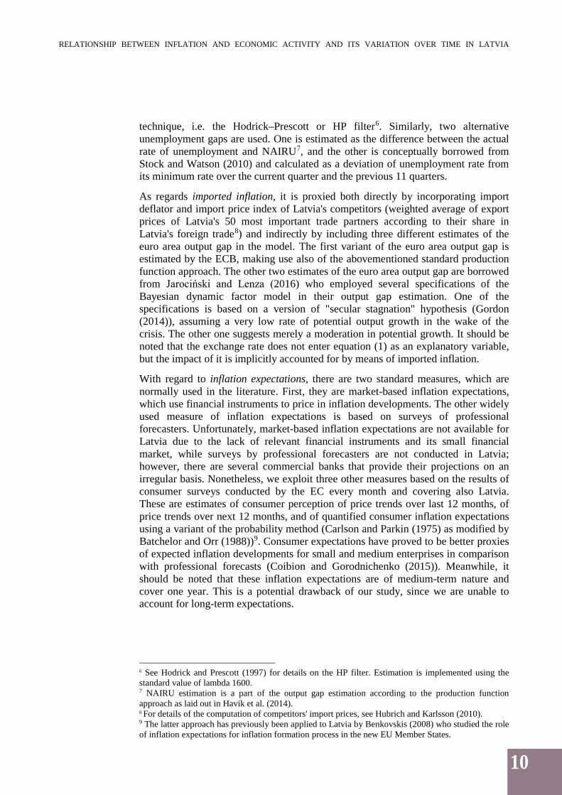
When discussing the relationship between inflation and economic slack, a broad set of slack measures is usually considered in different studies. They differ not only in terms of magnitude but also in the paths they follow. Output gap and unemployment gap, the most widely used economic slack measures, are well-known for being surrounded by a high degree of uncertainty, particularly in real time (see, for instance, Orphanides and van Norden (2002)). Their values also depend on the particular methodology chosen and are subject to frequent and large revisions ex-post. Therefore, in what follows we use these two unobservable measures of economic slack whose estimation involves employing different statistical de-trending or modelling techniques, and also readily available actual macroeconomic indicators. Two panels of Figure 2 accordingly display both unemployment and output related measures of slack and macroeconomic indicators. Speaking about two different output gap measures (one based on the HP filter, the other on the production function approach), they broadly follow a similar path. Largest discrepancy between the two was recorded at the outset of economic contraction in 2008. The production-function-based output gap was more prompt in signalling the looming crisis than the HP-based output gap. With regard to unemployment related slack measures, one should bear in mind that developments in unemployment rate may be of either structural or cyclical nature. Figure 2 shows that a steady decline in unemployment rate from the end-1990s until 2005 was of structural nature, as the unemployment gap fluctuated around zero. The gap turned negative, as the economy was booming, and changed the sign during the crisis on the back of worsening labour market conditions. Unemployment gap reached its peak in mid-2009, as the rate of unemployment jumped above 20%. Labour market appears to have been at its equilibrium at the end of 2014.

Figure 2 Developments in measures of Latvia's economic slack (year-on-year; %)

Sources: Eurostat and authors' calculations. Note: Data on unemployment recession gap are not available prior to 2000Q4.

40

45

50

55

60

65

70

75

80

–15

–10

–5

0

5

10

15

19

98

19

99

20

00

20

01

20

02

20

03

20

04

20

05

20

06

20

07

20

08

20

09

20

10

20

11

20

12

20

13

20

14

Output gap (HP)

Output gap (PF)

Capacity utilisation (%; right-hand scale)

–4

–2

0

2

4

6

8

0

4

8

12

16

20

24

19

98

19

99

20

00

20

01

20

02

20

03

20

04

20

05

20

06

20

07

20

08

20

09

20

10

20

11

20

12

20

13

20

14

Unemployment rate (%)

Unemployment recession gap (Stock and Watson (2010); %)

Unemployment gap (right-hand scale)

(a) Output-based (b) Unemployment-based


13

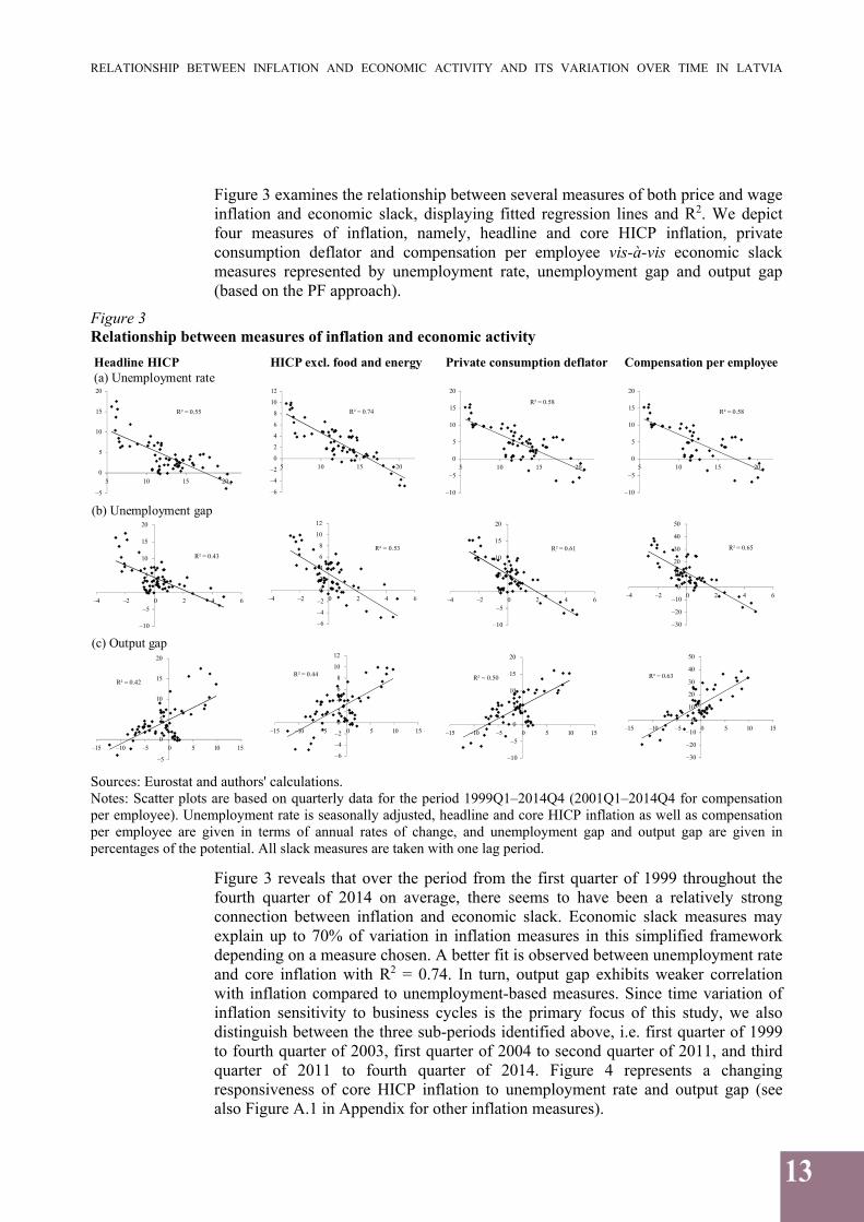
Figure 3 examines the relationship between several measures of both price and wage inflation and economic slack, displaying fitted regression lines and R2. We depict four measures of inflation, namely, headline and core HICP inflation, private consumption deflator and compensation per employee vis-à-vis economic slack measures represented by unemployment rate, unemployment gap and output gap (based on the PF approach).

Figure 3 Relationship between measures of inflation and economic activity

Sources: Eurostat and authors' calculations. Notes: Scatter plots are based on quarterly data for the period 1999Q1–2014Q4 (2001Q1–2014Q4 for compensation per employee). Unemployment rate is seasonally adjusted, headline and core HICP inflation as well as compensation per employee are given in terms of annual rates of change, and unemployment gap and output gap are given in percentages of the potential. All slack measures are taken with one lag period.

Figure 3 reveals that over the period from the first quarter of 1999 throughout the fourth quarter of 2014 on average, there seems to have been a relatively strong connection between inflation and economic slack. Economic slack measures may explain up to 70% of variation in inflation measures in this simplified framework depending on a measure chosen. A better fit is observed between unemployment rate and core inflation with R2 = 0.74. In turn, output gap exhibits weaker correlation with inflation compared to unemployment-based measures. Since time variation of inflation sensitivity to business cycles is the primary focus of this study, we also distinguish between the three sub-periods identified above, i.e. first quarter of 1999 to fourth quarter of 2003, first quarter of 2004 to second quarter of 2011, and third quarter of 2011 to fourth quarter of 2014. Figure 4 represents a changing responsiveness of core HICP inflation to unemployment rate and output gap (see also Figure A.1 in Appendix for other inflation measures).

R² = 0.55

–5

0

5

10

15

20

5 10 15 20

Headline HICP

R² = 0.74

–6

–4

–2

0

2

4

6

8

10

12

5 10 15 20

(a) Unemployment rate

HICP excl food and energy.

R² = 0.58

–10

–5

0

5

10

15

20

5 10 15 20

Private consumption deflator

R² = 0.58

–10

–5

0

5

10

15

20

5 10 15 20

Compensation per employee

R² = 0.43

–10

–5

0

5

10

15

20

–4 –2 0 2 4 6

R² = 0.53

–6

–4

–2

0

2

4

6

8

10

12

–4 –2 0 2 4 6

R² = 0.61

–10

–5

0

5

10

15

20

–4 –2 0 2 4 6

R² = 0.65

–30

–20

–10

0

10

20

30

40

50

–4 –2 0 2 4 6

(b) Unemployment gap

R² = 0.42

–5

0

5

10

15

20

–15 –10 –5 0 5 10 15

R² = 0.44

–6

–4

–2

0

2

4

6

8

10

12

–15 –10 –5 0 5 10 15

R² = 0.50

–10

–5

0

5

10

15

20

–15 –10 –5 0 5 10 15

R² = 0.63

–30

–20

–10

0

10

20

30

40

50

–15 –10 –5 0 5 10 15

(c) Output gap


14

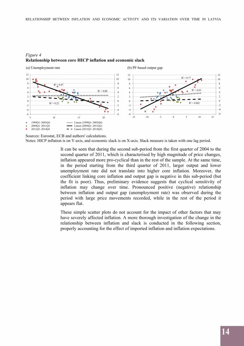
Figure 4 Relationship between core HICP inflation and economic slack

Sources: Eurostat, ECB and authors' calculations. Notes: HICP inflation is on Y-axis, and economic slack is on X-axis. Slack measure is taken with one lag period.

It can be seen that during the second sub-period from the first quarter of 2004 to the second quarter of 2011, which is characterised by high magnitude of price changes, inflation appeared more pro-cyclical than in the rest of the sample. At the same time, in the period starting from the third quarter of 2011, larger output and lower unemployment rate did not translate into higher core inflation. Moreover, the coefficient linking core inflation and output gap is negative in this sub-period (but the fit is poor). Thus, preliminary evidence suggests that cyclical sensitivity of inflation may change over time. Pronounced positive (negative) relationship between inflation and output gap (unemployment rate) was observed during the period with large price movements recorded, while in the rest of the period it appears flat.

These simple scatter plots do not account for the impact of other factors that may have severely affected inflation. A more thorough investigation of the change in the relationship between inflation and slack is conducted in the following section, properly accounting for the effect of imported inflation and inflation expectations.

R² = 0.00

R² = 0.87

R² = 0.22

–6

–4

–2

0

2

4

6

8

10

12

5 201510

–6

–4

–2

0

2

4

6

8

10

12

1999Q1–2003Q4

2004Q1–2011Q2

2011Q3–2014Q4

R² = 0.03

R² = 0.77

R² = 0.002

–15 –10 –5 0 5 10 15–6

–4

–2

0

2

4

6

8

10

12

–6

–4

–2

0

2

4

6

8

10

12

Linear (1999Q1–2003Q4)

Linear (2004Q1–2011Q2)

Linear (2011Q3–2014Q4)

(a) Unemployment rate (b) PF-based output gap


15

4. EMPIRICAL RESULTS

To investigate the variation of trade-off between inflation and economic slack, we conduct two exercises. In the first exercise, we estimate a large set of Phillips curves with time-invariant coefficients over two different samples and provide comparison of slack coefficients. In the second exercise, we allow the coefficients to vary over time by employing a more sophisticated estimation technique. The latter's advantage over the first approach is related to using the Bayesian estimation technique, which is particularly suitable for small samples. It also allows evaluation of the slack coefficient for each point of time throughout the sample employed in the study. Hence, the second exercise adds to greater robustness of the results of the first exercise. Finally, we bring more evidence on determinants of time variation of the slack coefficient.

4.1 Phillips curve with time-invariant (fixed) coefficients

We estimate 200 equations per each domestic inflation measure, accounting for all the variants of slack measures, imported inflation and inflation expectation indicators as described in Table 1 above. We discuss coefficients of other explanatory variables only slightly, as in the context of the current study they are of minor importance.

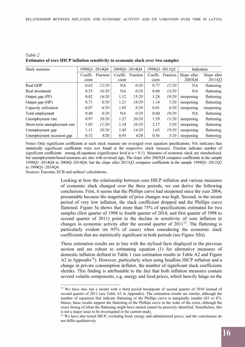
In the models with core HICP11 inflation as dependent variable estimated for all three samples (whole sample from the first quarter of 1998 to the fourth quarter of 2014 and two sub-samples from the first quarter of 1998 to the second quarter of 2011, and from the first quarter of 2004 to the fourth quarter of 2014), economic slack measures appear to be statistically significant in the majority of cases when unemployment gap, output gap (estimated using PF approach) or unemployment rate are used (see Table 2). In turn, the capacity utilisation and unemployment recession gap appear insignificant in more than half of the specifications across these three time spans. The statistical fit of the HP filter-based output gap is weaker in comparison with the PF-based one12. The magnitude of inflation sensitivity with respect to economic slack varies significantly across different slack measures13, with the largest reaction estimated with respect to unemployment gap and unemployment rate.

The inflation expectations coefficient is significant in the majority of specifications, particularly in the long sample and especially when the inflation expectations measure is calculated using the Carlson and Parkin's approach (1975). Surprisingly, imported inflation appears insignificant in many cases, although it does not mean that Latvia's domestic inflation is not affected by global inflationary pressures. Global inflation might have an impact on Latvia's inflation over an extended period of time, which is not captured by the single lag we account for in this study14.

11 We consider core HICP inflation as a benchmark inflation measure in our regressions due to its closer proximity to the real domestic activity. 12 The poor result for HP-filtered output gap may reflect several drawbacks of using the HP filter to derive the potential level of output, including the end-point problem and uncertainty in choosing the appropriate value of lambda. 13 Since the measures of economic slack have been standardised and homogenised in terms of their sign before entering the regression, we can compare the magnitude of slack coefficients. 14 Detailed modelling results are available upon request.


16

Table 2 Estimates of core HICP inflation sensitivity to economic slack over two samples

Slack measure 1998Q1–2014Q4 2004Q1–2014Q4 1998Q1–2011Q2 Indication Coeffi-

cient Fraction Coeffi-

cientFraction Coeffi-

cientFraction Slope after

2003Q4 Slope after

2011Q2Real GDP 0.62 12/20 NA 0/20 0.77 12/20 NA flatteningReal investment 0.55 16/20 NA 0/20 0.60 14/20 NA flatteningOutput gap (PF) 0.82 16/20 1.12 15/20 1.28 19/20 steepening flatteningOutput gap (HP) 0.71 8/20 1.21 18/20 1.14 7/20 steepening flatteningCapacity utilisation –0.07 6/20 1.05 8/20 0.01 6/20 steepening steepeningTotal employment 0.40 6/20 NA 0/20 0.60 10/20 NA flatteningUnemployment rate 0.97 20/20 1.27 20/20 1.59 11/20 steepening flatteningShort-term unemployment rate 1.05 11/20 1.34 10/20 2.17 5/20 steepening flatteningUnemployment gap 1.11 20/20 1.45 14/20 1.63 19/20 steepening flatteningUnemployment recession gap 0.52 8/20 0.95 4/20 0.56 5/20 steepening flattening

Notes: Only significant coefficients at each slack measure are averaged over equation specifications. NA indicates that statistically significant coefficients were not found at the respective slack measure. Fraction indicates number of significant coefficients among all equations (significance level is α = 0.1). Measures of economic slack are standardised, but unemployment-based measures are also with reversed sign. The slope after 2003Q4 compares coefficients in the sample 1998Q1–2014Q4 to 2004Q–2014Q4, but the slope after 2011Q2 compares coefficients in the sample 1998Q1–2011Q2 to 1998Q1–2014Q4. Sources: Eurostat, ECB and authors' calculations.

Looking at how the relationship between core HICP inflation and various measures of economic slack changed over the three periods, we can derive the following conclusions. First, it seems that the Phillips curve had steepened since the year 2004, presumable because the magnitude of price changes was high. Second, in the recent period of very low inflation, the slack coefficient dropped and the Phillips curve flattened. Figure 5a shows that more than 75% of specifications estimated for two samples (first quarter of 1998 to fourth quarter of 2014, and first quarter of 1998 to second quarter of 2011) point to the decline in sensitivity of core inflation to changes in economic activity after the second quarter of 201115. The flattening is particularly evident (in 95% of cases) when considering the economic slack coefficients that are statistically significant in both periods (see Figure 5(b)).

These estimation results are in line with the stylised facts displayed in the previous section and are robust to estimating equation (1) for alternative measures of domestic inflation defined in Table 1 (see estimation results in Table A2 and Figure A2 in Appendix16). However, particularly when using headline HICP inflation and a change in private consumption deflator, the number of significant slack coefficients shrinks. This finding is attributable to the fact that both inflation measures contain several volatile components, e.g. energy and food prices, which heavily hinge on the

15 We have also run a model with a third period breakpoint of second quarter of 2010 instead of second quarter of 2011 (see Table A3 in Appendix). The estimation results are similar, although the number of equations that indicate flattening of the Phillips curve is marginally smaller (83 vs 87). Hence, these results support the flattening of the Phillips curve in the wake of the crisis, although the exact timing of when the flattening might have started cannot be precisely identified. Nonetheless, this is not a major issue to be investigated in the current study. 16 We have also tested HICP, excluding food, energy and administered prices, and the conclusions do not differ qualitatively.


17

developments in international commodity markets and are vaguely connected to the developments in domestic real activity. Also, the explanatory power as measured by adjusted R2 is considerably higher in the cases of both core HICP inflation and core HICP at constant tax rates (R2 exceeds 0.8 on average across all 200 specifications) as compared to other measures of inflation. The lowest explanatory power is recorded for private consumption deflator (R2 = 0.40 on average) and wage related inflation measures (R2 is around 0.3–0.4).

Figure 5 Change in sensitivity of core HICP inflation to various economic slack measures after 2011Q2

Sources: Eurostat, ECB and authors' calculations. Notes: Blue dots reflect coefficients of various slack measures in two samples of data. Clusters of dots below 45° line indicate that coefficients are lower in the full sample compared to the short sample and point at the flattening of the Phillips curve.

In a nutshell, the models estimated for core HICP inflation perform better than those estimated for other domestic inflation measures. Among economic slack indicators, in terms of fit, the best ones seem to be unemployment rate, unemployment gap and output gap (PF).

Despite our estimation results being overwhelmingly supportive for the Phillips curve flattening in the recent period, which is of ultimate interest for us, there might be legitimate concerns whether this decline in the slope is statistically significant. In order to address this concern, we have implemented two tests.

First, we employ the standard slope dummy approach allowing for different slopes of the Phillips curve in two different periods in equation (4). Thus we plug the dummy which is equal to 1 into equation (4) for all quarters after the second quarter of 2011, so that the slack coefficient in the third period is equal to β β′. For the period prior to and until the second quarter of 2011, we plug the dummy which is equal to 0, implying that the slack coefficient in both (first and second) periods isβ. If β′ is negative and statistically significant, we find evidence of statistical significance of the Phillips curve flattening: π c απ β β′dummy x ρπ γπ ε (4).

The results indicate that the change in the slope is statistically significant in 34 specifications; hence, the evidence in favour of the significance of previously identified flattening of the Phillips curve is not unambiguous. Nonetheless, the sign of the slope dummy, as expected, is negative in almost all cases, and, if there has been a change in the slack coefficient, it has indeed been in the direction of the

–1.0

–0.5

0.0

0.5

1.0

1.5

2.0

2.5

3.0

–1.5 –1.0 –0.5 0.0 0.5 1.0 1.5 2.0 2.5 3.0

sample: 1998Q1–2011Q2

sam

ple

:1

99

8Q

1–

20

14

Q4

45° line

–1.0

–0.5

0.0

0.5

1.0

1.5

2.0

2.5

3.0

–1.0 –0.5 0.0 0.5 1.0 1.5 2.0 2.5 3.0

sample: 1998Q1–2011Q2

sam

ple

:1998Q

1–2014Q

4

45° line

(a) All cases (b) Significant cases only


18

Phillips curve flattening17. Moreover, the third period consists of a relatively small number of observations, which may be responsible for low statistical significance of a negative change in the slope.

Second, we perform a test for structural break developed by Hansen (1992). Hansen's Lagrange Multiplier (LM) test statistics is used for checking the parameter joint stability (see Table A4 in Appendix). There are 36 Phillips curve specifications, for which we are able to reject null hypothesis of the stability of all the parameters jointly at 10% level, implying there is a structural break in one or more parameters18. Importantly, these specifications include herein best-performing measures of economic slack, i.e. output and unemployment gaps and unemployment rate.

Overall, the analysis in this section indicates the Phillips curve flattening after the crisis, and these results are robust across different inflation and slack measures. Unfortunately, they are not strongly supported by formal statistical tests. The weakness of statistical tests may also stem from a relatively short span, over which the Phillips curve has been flattening, thus reducing the power of conventional tests. Moreover, when a slope coefficient is found to be statistically significant, it is indeed found smaller when more recent observations are added. All in all, we may unambiguously conclude that, if there has been a change in the slope recently, it has been in the downward direction. No evidence in favour of steepening Phillips curve is uncovered.

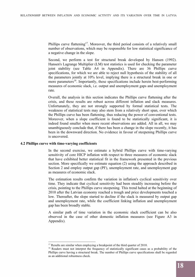
4.2 Phillips curve with time-varying coefficients

In the second exercise, we estimate a hybrid Phillips curve with time-varying sensitivity of core HICP inflation with respect to three measures of economic slack that have exhibited better statistical fit in the framework presented in the previous section. More specifically we estimate equation (2) using the approach described in Section 2 and employ output gap (PF), unemployment rate, and unemployment gap as measures of economic slack.

The estimation results confirm the variation in inflation's cyclical sensitivity over time. They indicate that cyclical sensitivity had been steadily increasing before the crisis, pointing to the Phillips curve steepening. This trend halted at the beginning of 2010 after the Latvian economy reached a trough and price developments touched a low. Thereafter, the slope started to decline if the slack is measured by output gap and unemployment rate, while the coefficient linking inflation and unemployment gap has been broadly stable.

A similar path of time variation in the economic slack coefficient can be also observed in the case of other domestic inflation measures (see Figure A3 in Appendix).

17 Results are similar when employing a breakpoint of the third quarter of 2010. 18 Readers must not interpret the frequency of statistically significant cases as a probability of the Phillips curve having a structural break. The number of Phillips curve specifications shall be regarded as an additional robustness check.


19

Figure 6 Time-varying sensitivity of core HICP inflation to three measures of economic slack

Sources: Eurostat, ECB and authors' calculations. Note: The figure shows median estimates of the slack coefficient for different slack measures together with 50% and 68% confidence intervals.

Our estimations suggest that slack coefficients may get higher as inflation rate grows and, on the contrary, as inflation becomes muted, slack coefficients shrink. This relationship between cyclical sensitivity of inflation and its average rate was actually suggested long ago. The seminal paper by Ball et al. (1988) attributed this relationship to the concept of "menu costs" of price adjustment, comprising both physical costs associated with printing new menus and price stickers as well as psychological costs of learning to think in "real" rather than "nominal" terms. As the general price level grows, menu costs decrease vis-à-vis losses incurred by sticking to the unchanged price level which starts deviating considerably from the profit maximising one. This leads to more frequent price revisions, implying that fluctuations in the economic activity are reflected in the price level more promptly. As inflation moderates and, in particular, as it enters a period of low levels, menu costs appear higher than possible losses from not reviewing prices. Therefore, firms may change prices less frequently when inflation is very low, particularly in the environment of weak competition. Ideally, we should look at the average frequency of price revision in the economy vis-à-vis the estimated slack coefficients, but there is no series on the frequency of price adjustment in Latvia long enough to incorporate it explicitly in a regression framework. Therefore, we start by testing whether slack coefficients and inflation estimated herein are interrelated and then examine the relationship between the slack coefficient and the frequency over a shorter time sample for which data are at our disposal.

0.10

0.15

0.20

0.25

0.30

0.35

0.40

0.45

0.50

0.55

1999 2001 2003 2005 2007 2009 2011

(a) Slope of the Phillips curve: output gap (PF)

0.10

0.15

0.20

0.25

0.30

0.35

0.40

0.45

0.50

0.55

2013

16–25

25–75

75–84

Median

–1.1

–1.0

–0.9

–0.8

–0.7

–0.6

–0.5

–0.4

–0.3

–0.2

(b) Slope of the Phillips curve: unemployment gap

–1.1

–1.0

–0.9

–0.8

–0.7

–0.6

–0.5

–0.4

–0.3

–0.2

1999 2001 2003 2005 2007 2009 2011 2013

–0.4

–0.3

–0.2

–0.1

0.0

0.1

0.2

(c) Slope of the Phillips curve: unemployment rate

1999 2001 2003 2005 2007 2009 2011 2013

–0.4

–0.3

–0.2

–0.1

0.0

0.1

0.2


20

4.3 Non-linearity of the Phillips curve and the role of price revision frequency

As mentioned above, an increase in the average inflation rate may cause firms to revise prices more frequently in order to meet rising costs, bringing about larger price flexibility and steeper Phillips curve. This explanation has been tested in the literature by authors employing either one-step approach (whereby an interaction term is included directly in the Phillips curve; see, for example, De Veirman (2009)), or two-step approach where the estimated slope of the Phillips curve (over time or across different countries) is regressed on average inflation or its standard deviation19 in a second-stage regression framework (as, for instance, in Ball et al. (1988) or Hess and Shin (1999)). There have also been attempts to explain variation in the slope of the Phillips curve by the measure of economic slack itself (see Laxton et al. (1995) and De Veirman (2009)) to account for the possible impact of capacity constraints or nominal rigidities on the inflation-economic slack trade-off. As the economy approaches its potential, further reduction in unemployment is difficult to achieve and that leads to accelerating inflation. Similarly, when unemployment gap widens considerably, deteriorating labour market conditions should result in nominal wage cuts and price reductions, which is highly unlikely if downward nominal rigidities are present. In other words, the presence of nominal rigidities/capacity constraints results in inflation growing faster when economic activity increases and declining at a slower pace during recessions.

In this study, we apply both the one-step approach for the Phillips curve with time-invariant coefficients (estimated in Subsection 4.1) and the two-step approach for the Phillips curve with time-varying coefficients (estimated in Subsection 4.2).

In the former case, we re-estimate equation (1) with the slack coefficient depending on the value of average inflation as reflected in equation (5) and depending on a slack measure as in equation (6). π c απ β β′π x ρπ γπ ε (5)

where the value of average inflation π is estimated as an 8-quarter moving average of actual inflation20. If β′ is positive and statistically significant, the inflation-economic activity trade-off depends on inflation itself in a fashion explained above. π c απ β β′′x x ρπ γπ ε (6).

If β′′ is positive21 and statistically significant, there might be reasons to suggest the presence of downward nominal rigidities.

19 As Ball et al. (1988) explains, inflation volatility may have an effect on the inflation-output trade-off similar to that of the average inflation. Increasing volatility of inflation raises uncertainty regarding the future path of optimal price level, leading to a more flexible approach to price setting and a steeper Phillips curve. However, in our study we already account for inflation volatility when estimating the Phillips curve by allowing the variance of the error to change over time. 20 De Veirman (2009) uses geometric average of 70 quarters of past inflation in a quarterly setting; Defina (1991) and Hess and Shin (1999) use 5-year moving average of current and past inflation in an annual setting. 21 Since the measures of economic slack have been homogenised in terms of their sign before entering the regression, both slack coefficient β and coefficient β are expected to be positive across all measures of economic slack.


21

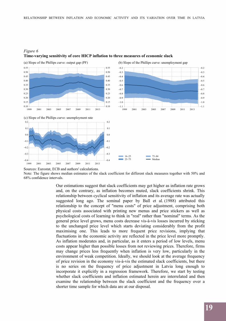
Table 3 shows that the number of statistically significant interactive dummies β′ with a correct positive sign is 70 for the value of average inflation and is considerably smaller (28 cases) for β′′when interaction with a measure of economic slack is included. Hence, the evidence in favour of average inflation and frequency of price revisions playing a role in driving the inflation-economic activity trade-off is stronger than in favour of the role of downward nominal rigidities.

Table 3 Estimates of core HICP inflation sensitivity to economic slack using average inflation and slack as determinants of slack coefficient

Slack measure Equation (4) Equation (5) Slack

coefficientCoefficient

(β')Fraction Slack

coefficient Coefficient

(β'') Fraction

Real GDP 0.22 0.08 0/0/20 0.45 0.07 0/9/20Real investment 0.00 0.18 18/0/20 0.59 0.17 12/16/20Output gap (PF) 0.81 0.06 1/13/20 0.72 0.13 0/15/20Output gap (HP) 0.71 0.03 0/12/20 0.49 0.06 0/7/20Capacity utilisation 0.37 0.18 4/0/20 0.42 0.15 0/3/20Total employment 0.06 0.12 4/0/20 0.12 0.00 0/0/20Unemployment rate 1.08 0.11 10/20/20 0.97 0.17 3/20/20Short-term unemployment rate 0.61 0.18 10/6/20 1.00 0.23 4/11/20Unemployment gap 0.80 0.11 12/15/20 1.17 0.11 1/20/20Unemployment recession gap 0.62 0.21 11/8/20 1.15 0.49 8/8/20

Notes: Coefficients at each slack measure are averaged over 20 different equation specifications. Fraction indicates number of significant interactive coefficients/number of significant slack coefficients/total number of equations (α = 0.1). Measures of economic slack are standardised, but unemployment-based measures are also with reversed sign.

Next, we turn to the framework of second-stage regression analysis. Using ordinary least squares, we regress time-varying slack coefficients estimated in Subsection 4.2 on average inflation π : π (7).

Again, we compute average inflation (π as an 8-quarter moving average of current and past core HICP inflation rates. It is likely, however, that the frequency of price revisions is not adjusted contemporaneously when the average inflation rate changes, as firms are not certain if this change in inflation is permanent or temporary. Hence, we also account for a lagged response of firms by estimating second-stage equations using the ARDL model methodology, which allows capturing the long-run effect of lagged values of inflation. We start with 4 lags (bearing in mind data availability constraints) and let the appropriate number of lags be chosen based on Akaike info criterion: π π (8). Hence, an advantage of the two-step approach is that it allows for the effect of trend inflation volatility to pass on to the slack coefficient through a gradual change in the price setting behaviour. The relationships we are testing below might also be non-linear, hence we include the squared values of trend inflation to test for non-linearity: π π (9).


22

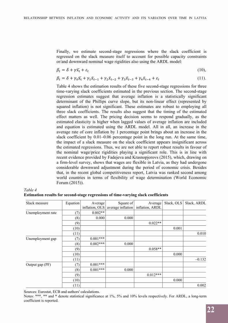
Finally, we estimate second-stage regressions where the slack coefficient is regressed on the slack measure itself to account for possible capacity constraints or/and downward nominal wage rigidities also using the ARDL model: x (10), x ̅ ̅ ̅ ̅ (11).

Table 4 shows the estimation results of these five second-stage regressions for three time-varying slack coefficients estimated in the previous section. The second-stage regression estimates suggest that average inflation is a statistically significant determinant of the Phillips curve slope, but its non-linear effect (represented by squared inflation) is not significant. These estimates are robust to employing all three slack coefficients. The results also suggest that the timing of the estimated effect matters as well. The pricing decision seems to respond gradually, as the estimated elasticity is higher when lagged values of average inflation are included and equation is estimated using the ARDL model. All in all, an increase in the average rate of core inflation by 1 percentage point brings about an increase in the slack coefficient by 0.01–0.06 percentage point in the long run. At the same time, the impact of a slack measure on the slack coefficient appears insignificant across the estimated regressions. Thus, we are not able to report robust results in favour of the nominal wage/price rigidities playing a significant role. This is in line with recent evidence provided by Fadejeva and Krasnopjorovs (2015), which, drawing on a firm-level survey, shows that wages are flexible in Latvia, as they had undergone considerable downward adjustment during the period of economic crisis. Besides that, in the recent global competitiveness report, Latvia was ranked second among world countries in terms of flexibility of wage determination (World Economic Forum (2015)).

Table 4 Estimation results for second-stage regressions of time-varying slack coefficients

Slack measure Equation Average inflation, OLS

Square of average inflation

Average inflation, ARDL

Slack, OLS Slack, ARDL

Unemployment rate (7) 0.002** (8) 0.000 0.000 (9) 0.022**

(10) 0.001 (11) 0.010

Unemployment gap (7) 0.001*** (8) 0.002*** 0.000 (9) 0.058**

(10) 0.000 (11) –0.132

Output gap (PF) (7) 0.001*** (8) 0.001*** 0.000 (9) 0.012***

(10) 0.000 (11) 0.002

Sources: Eurostat, ECB and authors' calculations. Notes: ***, ** and * denote statistical significance at 1%, 5% and 10% levels respectively. For ARDL, a long-term coefficient is reported.


23

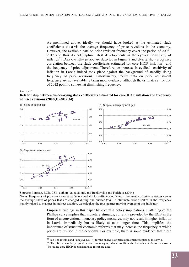
As mentioned above, ideally we should have looked at the estimated slack coefficients vis-à-vis the average frequency of price revisions in the economy. However, the available data on price revision frequency cover the period of 2003–2012 and thus do not capture latest developments in the cyclical sensitivity of inflation22. Data over that period are depicted in Figure 7 and clearly show a positive correlation between the slack coefficients estimated for core HICP inflation23 and the frequency of price adjustment. Therefore, an increase in cyclical sensitivity of inflation in Latvia indeed took place against the background of steadily rising frequency of price revisions. Unfortunately, recent data on price adjustment frequency are not available to bring more evidence, although the estimates at the end of 2012 point to somewhat diminishing frequency.

Figure 7 Relationship between time-varying slack coefficients estimated for core HICP inflation and frequency of price revisions (2003Q1–2012Q4)

Sources: Eurostat, ECB, CSB, authors' calculations, and Benkovskis and Fadejeva (2014). Notes: Frequency of price revisions is on X-axis and slack coefficient on Y-axis. Frequency of price revisions shows the average share of prices that are changed during one quarter (%). To eliminate erratic spikes in the frequency mainly related to changes in indirect taxation, we calculate the four-quarter moving average of this indicator.

Empirical findings in this paper have certain policy implications. Flattening of the Phillips curve implies that monetary stimulus, currently provided by the ECB in the form of unconventional monetary policy measures, may not result in higher inflation in Latvia immediately but is likely to take longer time. This amplifies the importance of structural economic reforms that may increase the frequency at which prices are revised in the economy. For example, there is some evidence that these 22 See Benkovskis and Fadejeva (2014) for the analysis of price adjustment frequency in Latvia. 23 The fit is similarly good when time-varying slack coefficients for other inflation measures (including core HICP at constant taxe rates) are used.

R² = 0.40

0.20

0.25

0.30

0.35

0.40

0.20 0.25 0.30 0.35 0.40

(a) Slope at output gap

R² = 0.88

0.40

0.50

0.60

0.70

0.80

0.90

0.20 0.25 0.30 0.35 0.400.20

0.25

0.30

0.35

0.40

0.40

0.50

0.60

0.70

0.80

0.90

R² = 0.76

0.00

0.05

0.10

0.15

0.20

0.25

0.00

0.05

0.10

0.15

0.20

0.25

(c) Slope at unemployment rate

(b) Slope at unemployment gap

0.20 0.25 0.30 0.35 0.40


24

reforms may appear particularly efficient in Latvia's services sector. Mark-ups in this sector are among the highest in the EU (see Table 1 in Varga and in 't Veld (2014)), especially in retail trade and the inland transport sector (see Table 2a in Thum-Thysen and Canton (2015)). It was also shown by Fadejeva and Krasnopjorovs (2015) that firms in the trade and business services sectors, where the frequency of price adjustment has recently declined, claim weaker competition to be the most important factor behind this development. Furthermore, Latvia got a relatively low score for the extent of market dominance in the latest global competitiveness report (World Economic Forum (2015)). This score has worsened over few recent years, with Latvia falling from the 51st position in 2011 to the 64th in 2014, and to the 61st in 2015 in the total ranking. All in all, some of the indicators presented above point towards a possible lack of competition in the domestic goods and services market. Hence, structural reforms aimed at strengthening competition and price flexibility in the services market, inter alia making it easier for foreign companies to operate in Latvia, could trigger more frequent adjustment of prices to changing economic environment, with prices responding to economic slack more rapidly.


25

CONCLUSIONS

This paper studies the relationship between Latvia's domestic inflation measures and economic slack, with a focus on time variation in this relationship employing two different but complementary approaches.

The evidence suggests that Phillips curve in Latvia might have been flattening in the wake of the crisis. The estimation results of the fixed coefficient approach indicate that the Phillips curve flattened after 2011; they are robust across different inflation and slack measures, albeit not strongly supported by formal statistical tests. The time-varying coefficient approach also points to a flattening Phillips curve, though the evidence is weak for some of the slack measures. All in all, we may unambiguously conclude that if there has been a change in the slope recently, it has been in the downward direction. No evidence in favour of steepening Phillips curve has been uncovered in this study.

Time variation in the economic slack coefficient could be associated with a change in price revision frequency. We show that steepening of the Phillips curve in Latvia had indeed been concomitant with an increase in the frequency of price changes. However, we have no data on the frequency of price revisions after 2012. Therefore, the connection between the slope and the frequency of price revisions remains somewhat uncertain and should be further investigated. This in turn requires the use of a richer dataset of consumer price micro data.

From the economic policy point of view, reduced inflation-economic slack trade-off implies that more remarkable improvements in economic activity are needed to bring inflation upwards, which requires a greater effort from the monetary policy of central banks. This amplifies the importance of structural economic reforms aimed at boosting competition and price flexibility. However, there is an important caveat when interpreting the results provided in the study. Even though the direct effect of a large drop in energy and other commodity prices is excluded when analysing the core HICP inflation, it may exert a negative indirect effect on core inflation. If this effect turns significant, it may partly explain low inflation amid positive economic slack. Further investigation of the indirect effect of energy prices on inflation is needed. To enhance our understanding of price setting strategies of firms, it is also important to gain insights into microeconomic consumer price data, including across different sectors and modes of trade. These may constitute the agenda of further research on inflation in Latvia.


26

APPENDIX

Estimation of the Phillips curve with time-varying parameters

The Phillips curve model with time-varying parameters is given in equations (A1–A7): π c α π β x ρ π γ π e ε (A1),

(A2),

(A3),

(A4),

(A5),

(A6),

(A7)

where is inflation, is slack measure, is the term capturing inflation expectations, is the proxy for imported inflation; , , , , and are time-varying parameters of the model and follow a random walk; , , , , and are unobserved shocks.

The model is estimated using the Bayesian technique. Since the model is quite complicated and there is no analytical solution, the Gibbs sampler similar to that of Primiceri (2005) is employed to draw posterior distribution of parameters. We run 20 000 iterations and burn-in 30% of them for posterior inference. The Bayesian methods require specifying prior distributions on the parameters of the model. We use inverse-gamma distribution for priors, where parameters are , , , , ~IG (5; 0.005), ~IG (5; 0.5). This parametrisation assumes that coefficients barely move over time, but log-volatility is expected to capture more variation.

Figure A1 Responsiveness of various domestic inflation measures to unemployment rate and output gap Panel A. Relationship between headline HICP inflation and economic slack

Sources: Eurostat, ECB and authors' calculations. Notes: Headline HICP inflation is on Y-axis and economic slack is on X-axis. Slack measure is taken with one lag period.

R² = 0.00

R² = 0.72

R² = 0.77

–15 –10 –5 0 5 10 15

–15

–10

–5

0

5

10

15

20

–15

–10

–5

0

5

10

15

20

R² = 0.02

R² = 0.74

R² = 0.66–5

0

5

10

15

20

5 10 15 20

–5

0

5

10

15

20

1999Q1–2003Q4

2004Q1–2011Q2

2011Q3–2014Q4

Linear (1999Q1–2003Q4)

Linear (2004Q1–2011Q2)

Linear (2011Q3–2014Q4)



27

Panel B. Relationship between private consumption deflator and economic slack

Sources: Eurostat, ECB and authors' calculations. Notes: Private consumption deflator is on Y-axis and economic slack is on X-axis. Slack measure is taken with one lag period.

Panel C. Relationship between compensation per employee and economic slack

Sources: Eurostat, ECB and authors' calculations. Notes: Compensation per employee is on Y-axis and economic slack is on X-axis. Slack measure is taken with one lag period. Data on compensation per employee start with 2001Q1, therefore the first period lasts 2001Q1–2003Q4.

R² = 0.28

R² = 0.74

R² = 0.73

–10

–5

0

5

10

15

20


1999Q1–2003Q4

2004Q1–2011Q2

2011Q3–2014Q4

Linear (1999Q1–2003Q4)

Linear (2004Q1–2011Q2)

Linear (2011Q3–2014Q4)

R² = 0.17

R² = 0.79

R² = 0.74

5

1–5 –1 0 5 10 15

–10

–5

0

5

10

15

20

5 10 15 20

–20

–15

–10

–5

0

5

10

15

20

25

30

–20

–15

–10

–5

0

5

10

15

20

25

30

R² = 0.13

R² = 0.70

R² = 0.51

–30

–20

–10

0

10

20

30

40

50

5 10 15 20


1999Q1–2003Q4

2004Q1–2011Q2

2011Q3–2014Q4

Linear (1999Q1–2003Q4)

Linear (2004Q1–2011Q2)

Linear (2011Q3–2014Q4)

–30

–20

–10

0

10

20

30

40

50

R² = 0.07

R² = 0.75

R² = 0.46

–15 –10 –5 0 5 10 15

–30

–20

–10

0

10

20

30

40

50

–30

–20

–10

0

10

20

30

40

50


28

Table A1 List of variables

Variable Source Time period Transformation Headline HICP (index: 2005 = 100; seasonally adjusted)

Eurostat 1998Q1–2014Q4 Annualised q-o-q growth rate

HICP excluding food and energy (index: 2005 = 100; seasonally adjusted)


HICP excluding food and energy at constant tax rates (index: 2005 = 100; seasonally adjusted)


Private consumption deflator (index: 2010 = 100; seasonally adjusted)


Compensation per employee (thousands of EUR; seasonally adjusted)

Eurostat, Latvijas Banka calculations

2000Q1–2014Q4 Annualised q-o-q growth rate

Compensation per hour (thousands of EUR; seasonally adjusted)

Eurostat, Latvijas Banka calculations

2002Q1–2014Q4 Annualised q-o-q growth rate

GDP at market prices (millions of EUR; chain-linked volumes (2010); seasonally and calendar adjusted)


Private investments at market prices (millions of EUR; chain-linked volumes (2010); seasonally and calendar adjusted)


Output gap (PF-based); deviation from potential output; %)

Latvijas Banka calculations 1998Q1–2014Q4 No

Output gap (HP filter-based); deviation from potential output; %)

Authors' calculations 1998Q1–2014Q4 No

Capacity utilisation (% of total capacity) EC 1998Q1–2014Q4 No Total employment (national accounts concept; thousands of persons)


Short-term unemployment rate (LFS data; % of economically active population (15–74) unemployed for up to one year)

Eurostat 2002Q1–2014Q4 No

Unemployment rate (LFS data; % of economically active population, 15–74)

Eurostat 1998Q1–2014Q4 No

Unemployment gap (deviation from NAIRU; %) Latvijas Banka calculations 1998Q1–2014Q4 No Unemployment recession gap (the difference between the current unemployment rate and the minimum rate in the current and past 11 quarters)

Authors' calculations based on Stock and Watson (2010)

2000Q4–2014Q4 No

Import deflator (index: 2010 = 100; seasonally adjusted)

Eurostat 1998Q1–2014Q4 Annual growth rate

Competitors' import prices (index: 2010 = 100; seasonally adjusted)

ECB 1998Q1–2014Q4 Annual growth rate

Euro area output gap (deviation from potential output; %)

ECB calculations 1998Q1–2014Q4 No

Euro area output gap (Jarociński and Lenza (2016); deviation from potential output; %)

ECB calculations based on Jarociński and Lenza (2016)

1998Q1–2014Q4 No

Past inflation (headline HICP; index: 2005 = 100; not seasonally adjusted)

Eurostat 1998Q1–2014Q4 Average of past four quarters of HICP annual rate of change

Consumer survey-based inflation expectations (annual inflation rate)

Authors' calculations based on Carlson and Parkin (1975)

1998Q1–2014Q4 No


29

Variable Source Time period Transformation Consumer survey-based price trends over last 12 months (balances; %)

EC 1998Q1–2014Q4 No

Consumer survey-based price trends over next 12 months (balances; %)

EC 1998Q1–2014Q4 No

Note: Prior to running the exercise with time-invariant coefficients slack measures are standardised, but unemployment-based measures are taken with a reversed sign.

Table A2 Estimates of domestic inflation sensitivity to economic slack over three samples

Panel A. Headline HICP inflation





2003Q4 Slope after

2011Q2Real GDP 0.69 10/20 0.82 1/20 0.89 10/20 steepening flatteningReal investment NA 0/20 NA 0/20 NA 0/20 NA NAOutput gap (PF) 1.03 5/20 1.29 2/20 1.74 10/20 steepening flatteningOutput gap (HP) 0.91 3/20 1.60 2/20 1.42 9/20 steepening flatteningCapacity utilisation –0.33 4/20 –1.33 4/20 1.05 1/20 steepening flatteningTotal employment NA 0/20 NA 0/20 NA 0/20 NA NAUnemployment rate 1.02 5/20 1.40 1/20 1.37 6/20 steepening flatteningShort-term unemployment rate –1.17 2/20 –1.61 2/20 –0.12 4/20 steepening steepeningUnemployment gap 1.05 4/20 1.15 2/20 1.70 4/20 steepening flatteningUnemployment recession gap –0.77 6/20 –1.08 2/20 –1.96 9/20 steepening flattening

Notes: Only significant coefficients at each slack measure are averaged over equation specifications. NA indicates that statistically significant coefficients were not found at the respective slack measure. Fraction indicates number of significant coefficients among all equations (significance level is α = 0.1). Measures of economic slack are standardised, but unemployment-based measures are also with reversed sign. The slope after 2003Q4 compares coefficients in the sample 1998Q1–2014Q4 to 2004Q1–2014Q4, but the slope after 2011Q2 compares coefficients in the sample 1998Q1–2011Q2 to 1998Q1–2014Q4.

Panel B. Core HICP inflation (at constant tax rates)





2003Q4 Slope after

2011Q2Real GDP 0.69 13/20 0.85 7/20 0.94 11/20 steepening flatteningReal investment NA 0/20 NA 0/20 NA 0/20 NA NAOutput gap (PF) 1.21 20/20 1.52 19/20 1.74 19/20 steepening flatteningOutput gap (HP) 0.79 14/20 1.15 13/20 1.49 10/20 steepening flatteningCapacity utilisation 0.87 15/20 1.26 12/20 1.29 10/20 steepening flatteningTotal employment NA 0/20 –0.79 10/20 NA 0/20 NA NAUnemployment rate 1.16 13/20 1.48 8/20 2.02 9/20 steepening flatteningShort-term unemployment rate 1.16 10/20 1.52 12/20 2.05 7/20 steepening flatteningUnemployment gap 1.13 15/20 1.38 13/20 1.62 13/20 steepening flatteningUnemployment recession gap 0.72 7/20 1.15 10/20 NA 0/20 steepening NA

Notes: Only significant coefficients at each slack measure are averaged over equation specifications. NA indicates that statistically significant coefficients were not found at the respective slack measure. Fraction indicates number of significant coefficients among all equations (significance level is α = 0.1). Measures of economic slack are standardised, but unemployment-based measures are also with reversed sign. The slope after 2003Q4 compares


30

coefficients in the sample 1998Q1–2014Q4 to 2004Q1–2014Q4, but the slope after 2011Q2 compares coefficients in the sample 1998Q1–2011Q2 to 1998Q1–2014Q4.

Panel C. Private consumption deflator





2003Q4 Slope after

2011Q2Real GDP 1.84 3/20 0.82 1/20 2.31 1/20 flattening flatteningReal investment 1.63 3/20 NA 0/20 1.94 2/20 NA flatteningOutput gap (PF) 2.44 5/20 1.29 2/20 4.65 5/20 flattening flatteningOutput gap (HP) 2.31 3/20 1.60 2/20 4.30 3/20 flattening flatteningCapacity utilisation 1.51 7/20 –1.33 4/20 4.37 5/20 flattening flatteningTotal employment NA 0/20 NA 0/20 NA 0/20 NA NAUnemployment rate 2.84 5/20 1.40 1/20 2.57 8/20 flattening steepeningShort-term unemployment rate 2.43 4/20 –1.61 2/20 3.00 5/20 flattening flatteningUnemployment gap 2.54 6/20 1.15 2/20 3.95 7/20 flattening flatteningUnemployment recession gap NA 0/20 –1.08 2/20 0.04 4/20 NA NA


Panel D. Compensation per employee





2003Q4 Slope after

2011Q2Real GDP 6.10 20/20 6.59 20/20 7.09 20/20 steepening flatteningReal investment 2.96 1/20 NA 0/20 NA 0/20 NA NAOutput gap (PF) 6.11 7/20 7.03 4/20 9.52 6/20 steepening flatteningOutput gap (HP) 4.34 4/20 6.14 2/20 8.04 4/20 steepening flatteningCapacity utilisation 4.80 12/20 7.13 8/20 6.27 7/20 steepening flatteningTotal employment 3.29 8/20 4.24 6/20 4.40 4/20 steepening flatteningUnemployment rate 7.82 5/20 8.68 5/20 15.41 5/20 steepening flatteningShort-term unemployment rate 5.39 5/20 6.51 4/20 13.47 2/20 steepening flatteningUnemployment gap 5.28 5/20 6.16 3/20 8.46 5/20 steepening flatteningUnemployment recession gap 3.74 2/20 6.40 4/20 5.75 2/20 steepening flattening



31

Panel E. Compensation per hour





2003Q4 Slope after

2011Q2Real GDP 7.57 20/20 8.77 15/20 9.79 20/20 steepening flatteningReal investment NA 0/20 NA 0/20 NA 0/20 NA NAOutput gap (PF) 5.74 2/20 7.28 1/20 9.15 2/20 steepening flatteningOutput gap (HP) NA 0/20 NA 0/20 –13.86 1/20 NA NACapacity utilisation 5.91 3/20 6.18 1/20 10.90 1/20 steepening flatteningTotal employment 5.43 7/20 6.26 6/20 8.59 7/20 steepening flatteningUnemployment rate 8.06 5/20 9.10 4/20 17.88 4/20 steepening flatteningShort-term unemployment rate 6.33 3/20 7.05 2/20 14.03 4/20 steepening flatteningUnemployment gap 5.58 1/20 6.59 1/20 NA 0/20 steepening NAUnemployment recession gap 5.82 4/20 7.56 3/20 10.63 4/20 steepening flattening


Table A3 Estimates of domestic inflation sensitivity to economic slack

Slack measure Sample: 1998Q1–2010Q2 1998Q1–2014Q4 IndicationCoefficient Fraction Coefficient Fraction

Real GDP 0.84 11/20 0.62 12/20 flatteningReal investment 0.61 14/20 0.55 16/20 flatteningOutput gap (PF) 1.26 17/20 0.82 16/20 flatteningOutput gap (HP) 1.06 7/20 0.71 8/20 flatteningCapacity utilisation –0.17 5/20 –0.07 6/20 flatteningTotal employment 0.63 7/20 0.40 6/20 flatteningUnemployment rate 1.73 10/20 0.97 20/20 flatteningShort-term unemployment rate 2.35 7/20 1.05 11/20 flatteningUnemployment gap 1.80 19/20 1.11 20/20 flatteningUnemployment recession gap –0.07 4/20 0.52 8/20 steepening

Notes: Only significant coefficients at each slack measure are averaged over equations specifications. Fraction indicates number of significant coefficients in the equations (α = 0.1). Measures of economic slack are standardised, but unemployment-based measures are also with reversed sign.


32

Figure A2 Changes in sensitivity of five domestic inflation measures to various economic slack measures after 2011Q2

sample: 1998Q1–2011Q2

sam

ple

:1998Q

1–2014Q

4

sample: 1998Q1–2011Q2

sam

ple

:1998Q

1–2014Q

4

Headline HeadlineHICP inflation (all coefficients) HICP inflation (significant coefficients only)

–4.0

–3.0

–2.0

–1.0

0.0

1.0

2.0

3.0

–4.0 –3.0 –2.0 –1.0 0.0 1.0 2.0 3.0

–4.0

–3.0

–2.0

–1.0

0.0

1.0

2.0

3.0

–4.0 –3.0 –2.0 –1.0 0.0 1.0 2.0 3.0

45° line

45° line

sample: 1998Q1–2011Q2

sam

ple

:1

99

8Q

1–

20

14

Q4

sample: 1998Q1–2011Q2

sam

ple

:1998Q

1–2014Q

4

Core CoreHICP inflation (at constant tax rates; all coefficients) HICP inflation (at constant tax rates; significant

coefficients only)

–3.0

–2.0

–1.0

0.0

1.0

2.0

3.0

4.0

–3.0 –2.0 –1.0 0.0 1.0 2.0 3.0 4.0

–1.0

–0.5

0.0

0.5

1.0

1.5

2.0

2.5

3.0

3.5

4.0

–1.0 –0.5 0.0 0.5 1.0 1.5 2.0 2.5 3.0 3.5 4.0

45° line

45° line

sample: 1998Q1–2011Q2

sam

ple

:1

99

8Q

1–

20

14

Q4

sample: 1998Q1–2011Q2

sam

ple

:1998Q

1–2014Q

4

Headline inflation (all coefficients) Headline inflation (significant coefficients only)HICP HICP

–4.0

–2.0

0.0

2.0

4.0

6.0

8.0

–8.0 –6.0 –4.0 –2.0 0.0 2.0 4.0 6.0 8.0

–1.0

0.0

1.0

2.0

3.0

4.0

5.0

6.0

7.0

8.0

–1.0 0.0 1.0 2.0 3.0 4.0 5.0 6.0 7.0 8.0

45° line

45° line

–5.0

0.0

5.0

10.0

15.0

20.0

–20.0 –15.0 –10.0 –5.0 0.0 5.0 10.0 15.0 20.0

sample: 1998Q1–2011Q2

sam

ple

:1

99

8Q

1–

20

14

Q4

sample: 1998Q1–2011Q2

sam

ple

:1998Q

1–2014Q

4

Compensation per hour (all coefficients) Compensation per hour (significant coefficients only)

0.0

5.0

10.0

15.0

20.0

0.0 5.0 10.0 15.0 20.0

45° line 45° line


33

Notes: Blue dots reflect coefficients of various slack measures in two samples of data. Clusters of dots below the 45° line indicate that coefficients are lower in the full sample compared with the short sample and point at flattening of the Phillips curve.

Table A4 Results of Hansen's LM test for parameter instability

1% crit 5% crit 10% critReal GDP 0/20 0/20 0/20Real investment 0/20 0/20 0/20Output gap (PF) 3/20 2/20 1/20Output gap (HP) 0/20 4/20 2/20Capacity utilisation 0/20 1/20 2/20Total employment 0/20 0/20 1/20Unemployment rate 1/20 5/20 0/20Short-term unemployment rate 0/20 2/20 1/20Unemployment gap 1/20 3/20 2/20Unemployment recession gap 0/20 3/20 2/20

Note: Null hypothesis tests for joint time invariance of all parameters in a model. Table shows fraction of equations at each slack measure where null hypotheses were rejected with specified level of statistical significance (denoted by crit).

–3.0

–1.0

1.0

3.0

5.0

7.0

9.0

11.0

13.0

15.0

–10.0 –5.0 0.0 5.0 10.0 15.0

sample: 1998Q1–2011Q2

sam

ple

:1998Q

1–2014Q

4

sample: 1998Q1–2011Q2

sam

ple

:1998Q

1–2014Q

4

Headline HeadlineHICP inflation (all coefficients) HICP inflation (significant coefficients only)

–5.0

–3.0

–1.0

1.0

3.0

5.0

7.0

9.0

11.0

13.0

15.0

–5.0 –3.0 –1.0 1.0 3.0 5.0 7.0 9.0 11.0 13.0 15.0

45° line

45° line


34

Figure A3 Time-varying sensitivity of various domestic inflation measures to three measures of economic slack Panel A. Headline HICP inflation

Panel B. Core HICP inflation at constant tax rates

Note: Figures represent the results of the Phillips curve specifications, which are selected among those with significant slack coefficients and the highest R2.

–0.15

–0.10

–0.05

0.00

0.05

0.10

0.15

0.20

0.25

0.30

0.35

(a) utput gapO (b) nemployment gapU

(c) nemployment rateU

16–25

25–75

75–84

Median

–0.15

–0.10

–0.05

0.00

0.05

0.10

0.15

0.20

0.25

0.30

0.35

1999 2001 2003 2005 2007 2009 2011 2013

–0.9

–0.8

–0.7

–0.6

–0.5

–0.4

–0.3

–0.2

–0.1

0.0

–0.9

–0.8

–0.7

–0.6

–0.5

–0.4

–0.3

–0.2

–0.1

0.0

1999 2001 2003 2005 2007 2009 2011 2013

–0.25

–0.20

–0.15

–0.10

–0.05

0.00

0.05

0.10

0.15

0.20

0.25

–0.25

–0.20

–0.15

–0.10

–0.05

0.00

0.05

0.10

0.15

0.20

0.25

1999 2001 2003 2005 2007 2009 2011 2013

0.0

0.1

0.2

0.3

0.4

0.5

0.6

0.7

0.8

(a) utput gapO (PF) (b) nemployment gapU

2001 2003 2005 2007 2009 2011 2013

0.0

0.1

0.2

0.3

0.4

0.5

0.6

0.7

0.8

–1.4

–1.2

–1.0

–0.8

–0.6

–0.4

–0.2

0.0

–1.4

–1.2

–1.0

–0.8

–0.6

–0.4

–0.2

0.0

2001 2003 2005 2007 2009 2011 2013


–0.5

–0.4

–0.3

–0.2

–0.1

0.0

0.1

–0.5

–0.4

–0.3

–0.2

–0.1

0.0

0.1

2001 2003 2005 2007 2009 2011 2013

16–25

25–75

75–84

Median


35

Panel C. Private consumption deflator

Note: Figures represent the results of the Phillips curve specifications, which are selected among those with significant slack coefficients and the highest R2.

–0.3

–0.2

–0.1

0.0

0.1

0.2

0.3

0.4

(b) nemployment gapU


16–25

25–75

75–84

Median

(a) utput gapO (PF)

–1.2

–1.0

–0.8

–0.6

–0.4

–0.2

0.0

0.2

–0.35

–0.30

–0.25

–0.20

–0.15

–0.10

–0.05

0.00

0.05

0.10

0.15

0.20

–0.35

–0.30

–0.25

–0.20

–0.15

–0.10

–0.05

0.00

0.05

0.10

0.15

0.20

1999 2001 2003 2005 2007 2009 2011 2013 1999 2001 2003 2005 2007 2009 2011 2013

1999 2001 2003 2005 2007 2009 2011 2013

–0.3

–0.2

–0.1

0.0

0.1

0.2

0.3

0.4

–1.2

–1.0

–0.8

–0.6

–0.4

–0.2

0.0

0.2


36

BIBLIOGRAPHY

ÁLVAREZ, Luis J., URTASUN, Alberto (2013). Variation in the Cyclical Sensitivity of Spanish Inflation: An Initial Approximation. Banco de España Economic Bulletin, July–August 2013, pp. 11–17. BALL, Laurence, MANKIW, Gregory N., ROMER, David (1988). The New Keynesian Economics and the Output-Inflation Trade-off. Brookings Papers on Economic Activity, vol. 19, issue 1, pp. 1–82. BATCHELOR, Roy, ORR, Adrian (1988). Inflation Expectations Revisited. Economica, vol. 55, issue 219, August 1988, pp. 317–331. BENKOVSKIS, Konstantins (2008). The Role of Inflation Expectations in the New EU Member States: Consumer Survey Based Results. Czech Journal of Economics and Finance, vol. 58, issue 7–8, pp. 298–317. BENKOVSKIS, Konstantins, FADEJEVA, Ludmila (2014). The Effect of VAT Rate on Inflation in Latvia: Evidence from CPI Microdata. Applied Economics, vol. 46, issue 21, April 2014, pp. 2520–2533. BESSONOVS, Andrejs, TKAČEVS, Oļegs (2015a). Kāpēc inflācija Latvijā ir tik zema? Latvijas Banka [viewed 7 June 2016]. Available from: https://www.makroekonomika.lv/kapec-inflacija-latvija-ir-tik-zema. BESSONOVS, Andrejs, TKAČEVS, Oļegs (2015b). What Are the Direct Effects of Oil Price Developments on Latvia's Inflation? Latvijas Banka Monthly Newsletter, January 2016. BLANCHARD, Olivier, CERUTTI, Eugenio, SUMMERS, Lawrence (2015). Inflation and Activity – Two Explorations and Their Monetary Policy Implications. NBER Working Paper, No. 21726, November 2015. 29 p. BORIO, Claudio, FILARDO, Andrew (2007). Globalisation and Inflation: New Cross-Country Evidence on the Global Determinants of Domestic Inflation. BIS Working Paper, No. 227, May 2007. 54 p. CALVO, Guillermo (1983). Staggered Prices in a Utility-Maximizing Framework. Journal of Monetary Economics, vol. 12, issue 3, September 1983, pp. 383–398. CARLSON, John A., PARKIN, Michael (1975). Inflation Expectations. Economica, vol. 42, issue 166, pp. 123–138. COIBION, Olivier, GORODNICHENKO, Yuriy (2015). Is the Phillips Curve Alive and Well after All? Inflation Expectations and the Missing Disinflation. American Economic Journal: Macroeconomics, vol. 7, No. 1, January 2015, pp. 197–232. DE VEIRMAN, Emmanuel (2009). What Makes the Output-Inflation Trade-Off Change? The Absence of Accelerating Deflation in Japan. Journal of Money, Credit and Banking, vol. 41, issue 6, pp. 1117–1140. DEFINA, Robert H. (1991). International Evidence on a New Keynesian Theory of the Output-Inflation Trade-off. Journal of Money, Credit and Banking, vol. 23, No. 3, Part 1, August 1991, pp. 410–422. ECB (2014). The Phillips Curve Relationship in the Euro Area. ECB Monthly Bulletin, July 2014, pp. 99–117.


37

ECB (2016). European Central Bank Annual Report 2015. 211 p. FADEJEVA, Ludmila, KRASNOPJOROVS, Oļegs (2015). Labour Market Adjustment during 2008–2013 in Latvia: Firm Level Evidence. Latvijas Banka Working Paper, No. 2/2015. 178 p. FRIEDMAN, Milton (1968). The Role of Monetary Policy. American Economic Review, vol. 58, No. 1, March 1968, pp. 1–17. GALÍ, Jordi, GERTLER, Mark (1999). Inflation Dynamics: A Structural Econometric Analysis. Journal of Monetary Economics, vol. 44, issue 2, October 1999, pp. 195–222. GORDON, Robert J. (2014). The Turtle's Progress: Secular Stagnation Meets the Headwinds. In: Secular Stagnation: Facts, Causes, and Cures. VoxEU.org ebook. CEPR Press, pp. 47–60. HANSEN, Bruce E. (1992). Testing for Parameter Instability in Linear Models. Journal of Policy Modeling, No. 14, issue 4, pp. 517–533. HAVIK, Karel, McMORROW, Kieran, ORLANDI, Fabrice, PLANAS, Christophe, RACIBORSKI, Rafal, RÖGER, Werner, ROSSI, Alessandro, THUM-THYSEN, Anna, VANDERMEULEN, Valerie (2014). The Production Function Methodology for Calculating Potential Growth Rates and Output Gaps. European Commission, European Economy, Economic Papers, No. 535, November 2014. 120 p. HESS, Gregory D., SHIN, Kwanho (1999). Some International Evidence on Output-Inflation Trade-Offs. Macroeconomic Dynamic, vol. 3, issue 2, June 1999, pp. 187–203.

HODRICK, Robert J., PRESCOTT, Edward C. (1997). Postwar U.S. Business Cycles: An Empirical Investigation. Journal of Money, Credit and Banking, vol. 29, No. 1, February 1997, pp. 1–16. HUBRICH, Kirstin, KARLSSON, Tohmas (2010). Trade Consistency in the Context of the Eurosystem Projection Exercises. An Overview. ECB Occasional Paper, No. 108, March 2010. 49 p. International Monetary Fund (2013). The Dog That Didn't Bark: Has Inflation Been Muzzled or Was It just Sleeping? In: World Economic Outlook, Chapter 3, April 2013, pp. 79–96. JAROCIŃSKI, Marek, LENZA, Michele (2016). An Inflation-predicating Measure of the Output Gap in the Euro Area. ECB Working Paper (forthcoming). 14 July 2016 version. 40 p. LAXTON, Douglas, MEREDITH, Guy, ROSE, David (1995). Asymmetric Effects of Economic Activity on Inflation: Evidence and Policy Implications. IMF Staff Papers, vol. 42, No. 2, June 1995, pp. 344–374. MEĻIHOVS, Aleksejs, ZASOVA, Anna (2007). Estimation of the Phillips Curve for Latvia. Latvijas Banka Working Paper, No. 3/2007. 28 p. MUSSO, Alberto, STRACCA, Livio, van DIJK, Dick (2009). Instability and Nonlinearity in the Euro-Area Phillips Curve. International Journal of Central Banking, vol. 5, No. 2, June 2009, pp. 181–212.


38

OINONEN, Sami, PALOVIITA, Maritta (2014). Updating the Euro Area Phillips Curve: The Slope Has Increased. Bank of Finland Research Discussion Paper, No. 31. 12 p. ORPHANIDES, Athanasios, van NORDEN, Simon (2002). The Unreliability of Output-Gap Estimates in Real Time. The Review of Economics and Statistics, vol. 84, issue 4, pp. 569–583. PHILLIPS, Alban William (1958). The Relation between Unemployment and the Rate of Change of Money Wage Rates in the United Kingdom, 1861–1957. Economica, vol. 25, issue 100, November 1958, pp. 283–299. PRIMICERI, Giorgio (2005). Time Varying Structural Vector Autoregressions and Monetary Policy. Review of Economic Studies, vol. 72, issue 3, pp. 821–852. RIGGI, Marianna, VENDITTI, Fabrizio (2014). Surprise! Euro Area Inflation Has Fallen. Banca d'Italia Ocassional Paper, No. 237, September 2014. 33 p. ROBERTS, John M. (2006). Monetary Policy and Inflation Dynamics. International Journal of Central Banking, vol. 2, No. 3, September 2006, pp. 193–230. STELLA, Andrea, STOCK, James H. (2012). A State-Dependent Model for Inflation Forecasting. Board of Governors of the Federal Reserve System International Finance Discussion Paper, No. 1062, October 2012. 25 p. STEVENS, Arnoud (2013). What Inflation Developments Reveal about the Phillips Curve: Implications for Monetary Policy. National Bank of Belgium Economic Review, December 2013, pp. 67–76. STOCK, James H., WATSON, Mark W. (2010). Modeling Inflation after the Crisis. NBER Working Paper, No. 16488, October 2010. 61 p. THUM-THYSEN, Anna, CANTON, Erik (2015). Estimation of Service Sector Mark-ups Determined by Structural Reform Indicators. European Commission, European Economy, Economic Papers 547, April 2015. 48 p. VARGA, Janos, IN 'T VELD, Jan (2014). The Potential Growth Impact of Structural Reforms in the EU: A Benchmarking Exercise. European Commission, European Economy, Economic Papers 541, December 2014. 40 p. World Economic Forum (2015). The Global Competitiveness Report 2015–2016. 403 p. [viewed 7 June 2016]. Available from: http://www3.weforum.org/docs/gcr/2015-016/Global_Competitiveness_Report_2015-2016.pdf.

Documents

Relationship Between Inflation and Economic Activity and ... · relationship between inflation and economic activity, particularly in some individual euro area countries. For example,