Relationship between Money Supply, Income and Price Level

NRB Working Paper No. 46

June 2019

Relationship between Money Supply, Income and

Price Level in Nepal#

Ram Chandra Acharya*

ABSTRACT

This paper intends to find out the relationship between money supply, income and price

level in Nepal using the data from the end of fiscal year 1974/75 to 2017/18. The paper

tries to establish the relationship between real money supply (both M1 and M2) and real

GDP, nominal money supply (both M1 and M2) and price level as well as nominal GDP

and price level separately. The econometric tools such as ADF for unit root tests, SIC for

lag length selection, bivariate Johansen Cointegration tests followed by VECM for long-

run causality, and VEC as well as VAR Granger Causality/Block Exogeneity Wald tests

for short-run causality are used in the study. The paper found that there is bidirectional

long-run casualty between the real income and both type of money supply in real terms.

But there is no evidence of short run causation between these variables. Likewise, the

study has found the unidirectional long-run relationship runs from narrow money supply

to consumer price. However, there is no short-run relationship from either side.

Accordingly, there is no evidence of long-run as well as short-run relationship between

broad money supply and consumer price level. Lastly, there is no evidence of long-run

causality between nominal GDP and general price level. But the study found the

unidirectional short-run causality running from general price to nominal GDP. The

results suggest that the Nepal should focus on steady growth of broad money supply (time

deposit rather than narrow money supply) in long-run for economic growth and control

of inflation both.

JEL Classification: E51, E31, C32

Key Words: Broad and Narrow Money Supply, Price level, Short-run and Long-run

Causality

# This paper is synthesized and upgraded version of the Master thesis of the author. The thesis was written

under the supervision of Assistant Prof. Mr. Khagendra Katuwal, CEDECON, TU. The author would like to

thank Mr. Katuwal, Dr. R. D. Singh (External Examiner), Prof. Dr. Kusum Shakya (Head of the CEDECON)

and Dr. Gunakar Bhatta (Executive Director, Reserch Department) for their continuous support from initial

phase of writing through the publication date. The author would like to thank all the supporter as well.

* Assistant Director, Nepal Rastra Bank. E-mail: [email protected]

© 2019 Nepal Rastra Bank

Relationship between Money Supply, Income and Price Level in Nepal NRBWP46

2

I. INTRODUCTION

The relationship between money, income and prices has been a subject of discussion among

economists for a long time. Specifically, the role of money in determination of income and

prices has been being debated extensively over the decades. According to the classicists, the

increase in money stock shifts up the aggregate demand without affecting the supply side

(Ackley, 2007). This increment on money supply leads to increase in price level which just

offsets the increase in nominal money, leaving the real money stock unchanged. Money, then,

is completely neutral in the classical economy, real output, income and other real variables

are completely left unchanged by change in the money supply (Branson, 2005).

Keynesians held the view that money does not play an active role in determining income and

prices. They stress on that the direction of causation runs from income to money without any

feedback (Al-Jarrah, 1996). According to their view changes in the stock of money supply

affects the interest rate and hence investment and consumption (Salih, 2013; Coddington,

1976). The effect goes through the income at last. They say changes in the stock of money

supply affects income only indirectly (Shapiro, 2001). Accordingly, changes in income cause

changes in the stock of money supply through change in the demand for money, given sticky

interest rates (Branson, 2005). This indicates a unidirectional causality from income to money

supply. Similarly, according to the Keynesians, prices are determined by the demand and

supply forces. In Keynesian point of view, inflation as a real phenomenon caused mainly by

real factors (Al-Jarrah, 1996; Blinder, 1988). The Keynesians economists negate the role of

money in the price change. They are of the view that changes in prices are mainly due to

structural factors (Ahmad, Asad and Hussian, 2008).

Contrary to the Keynesians, The Monetarists led by Milton Friedman faithfully claim that

money supply plays an active role in determining income and prices (Salih, 2013; Laidler,

1981). This indicates that both income and prices are mainly caused by changes in the stock

of money supply in the short-run (Froyen, 2014). Monetarists believe that the direction of

causation runs from money to income without any feedback only in the short-run and the

inflation is a monetary phenomenon in that changes in money supply cause changes of prices

in both short-run as well as long-run (Mayer, 1975). In clear notation, the monetarists'

proposition suggests that there is a unidirectional causality from money supply to income and

a unidirectional causality from money supply to prices.

The new classical point of view totally ignored the association between money supply and

income in both long-run and short-run because of rational expectation hypothesis (Froyen,

2014). Rather the overall effect of change in money supply remains only on price level

(Maddock & Carter, 1982). Their view coincides the view of classical.

The new Keynesian are giving the strong microeconomic foundation to the Keynesian system

(Froyen, 2014). So, they are in the supporting view to the Keynesian view of indirect

association between money supply, income and price (Gordon, 1990). But they are not so


3

much rigid like the early Keynesian to believe the effectiveness of monetary policy (Froyen,

2014).

Despite this clear dispute, it is very crucial to understand the relationship between the

variables such as; income, money and prices in an economy. Understanding this relationship

is important, especially to the public policymakers, in conducting effective stabilization

policies. The causal relationships between money and income as well as between money and

prices have been an active area of research in economics particularly after the publication of

the influential paper by Sims (1972). Based on Granger causality; Sims developed a test of

causality and applied it to data from the United States to examine the causal relationship

between money and income. He found the evidence of unidirectional causal relationship

running from money to income supporting the Monetarists’ claim (Salih, 2013).

The money supply, income and price level have increasing tendency over the years in Nepal.

The average increment rate of narrow money, broad money, GDP and price level over the last

43 years are 15.69, 18.65, 4.35 and 8.19 percent respectively. Accordingly, the average

growth rate of real narrow money and real broad money are 6.98 and 9.72 percent

respectively. These figures clearly show that all these macroeconomic variables are in

increasing trend. Therefore, there may be possibility of achieving the unidirectional or

bilateral causal relationship between money, price and income though the ideology differs

from one school to another (Gyanwaly, 2012). Hence, there might be long run as well as

short-run relationship between these variables. The relationship between these variables has

significant importance because it traces out the nexus between these variables and provides

policy implications to the policy makers (www.intelligenteconomist.com). So, the main task

of this study is to discuss and identify the casual relationship between these variables in the

latest context of Nepal.

Hence, the problem of this study can be synthesized in the following research question;

i. Is there any long-run and short-run relationship between these macroeconomic

variables?

So, the objective of the study is to find out the long run and short run relationship between

the money supply, income and the price level in Nepal.

There are few limitations of the study. First, there are methodological limitations of this

study. The conclusions drawn by this study may not be matched with the conclusions drawn

by the study which used another methodology. Secondly, the quarterly or monthly data are

usually needed for the dynamic analysis of the model, but because of the unavailability of

such data recorded in Nepal. This study is obliged to use the annual data which may lead the

less dynamic results. Third limitation of this study is that it covers only the data from 1975-

2018 of Nepal, which may not provide the conclusion for all. Another limitation of this study

is that it uses bivariate models to illustrate relationship between variables.


4

II. REVIEW OF LITERATURE

Friedman and Schwartz (1963) found that the changes in the behavior of the money stock had

been closely related with the changes in economic activity, money income, and prices in

American economy during the period from 1867 to 1960. They also found that the interaction

between monetary and economic change had been highly stable. However, they observed that

monetary changes often had an independent origin; they have not been simply a reflection of

changes in economic activity.

Al-Jarrah (1996) investigated the nature of the linkages between money, real income, and

prices in Saudi Arabia. The study used multivariate Johansen technique, Granger-causality

tests, and variance decomposition and impulse response functions to test for causal

relationships among variables. The results indicated that real income contributes significantly

in explaining changes in the money, while the reverse was not true. Consumer prices were

also significant in predicting changes in money in the Kingdom. The evidence on the

contribution of money in explaining prices change, however, was weak.

Holod (2000) investigated the relationships between the money supply, exchange rate and

prices in the Ukrainian economy by employing the monthly data from 1995:01 to 1999:06.

The study used vector autoregression (VAR), vector error correction model and impulse

response functions as its methodology to show how a shock in one of the variables influences

the time behavior of others. The paper found some evidence that money supply shocks

affected the price level behavior, but the effect was not very strong. On the other hand, the

paper found that the money supply responded significantly to the shocks in the price level.

Ahmad, Asad and Hussian (2008) used the time series data of real GDP, nominal GDP, prices

and money supply for the period of 1973 to 2007. The study used ADF to test the stationary

of the data series and series were found integrated of the order zero. The Granger causality

test was used for causal relationship. The paper found the estimated coefficient between the

growth of money supply and inflation positive and significant. The study accepted the

Monetarist proposition that money supply determined the price levels and income. The

authors suggested a tight monetary policy along with fiscal measures to control inflation in

Pakistan.

Ishan and Anjum (2013) described the main role of money supply (M2) on GDP of Pakistan.

The study used the secondary data of 12 years from 2000 to 2011. The paper found the

excessive money supply (M2) by SBP (State Bank of Pakistan) to run the country entails to

high rate of inflation if the indicators i.e. CPI, interest rate are not controlled within the

prescribed limits. The research found the evidence that high rate of inflation has adversely

affected the economy of Pakistan because of excessive supply of money (M2) by SBP. The

study revealed the impact of money supply (M2) on the GDP of Pakistan whereby the

country has seen inflation rate in double digits. By using regression model, the paper has

proved that Interest rate and CPI have a significant relation with GDP but inflation has no

significant relation with the GDP. Thus, they have suggested that the money supply needs

aggressive control to boost the economy.


5

Salih (2013) examined the relationship between the three macroeconomic variables money,

income, and prices in the Saudi Arabian economy. The methodology used in the paper is

cointegration, bivariate and trivariate Vector Autoregressive (VAR) models, and Granger

Causality/Block Exogeneity tests. The author further supplemented the results with impulse

response and variance decomposition. The results for Saudi Arabia for the period 1968-2011

indicated two-way causation between income and money supply. The results also showed

that income Granger causes prices, and money Granger causes money prices.

Luo (2013) investigated the money supply behavior (endogeneity or exogeneity) of BRICS

(Brazil, Russia, India, China, and South Africa) using quarterly data from 1982 to 2012. The

author used the econometric methodologies like Chow Breakpoint Test, Unit Root Test,

Johanson Cointegration Test, Granger causality Test, Vector Error Correction and Trivarite

Vector Autocorrelation Matrix for the thesis. In four countries: Brazil, China, Russia (the

period of 2004-2012) and South Africa (1982-1993), the study found money supply

endogeneity evidence. Thus, this implies that bank loans cause the money supply, or there is

bidirectional causality between these two. Regarding the other countries (India and the 1982-

2003 period of Russia) the thesis found money supply to be exogenous which means money

supply cause bank loans. The study concluded that in the short run; most of the countries

share at least some degree of the monetarist view which envisages exogeneity of money

supply.

Singh, Das and Baig (2015) examined the casual relationship between money supply, output

and prices of India in the short and long-term both. Different metrics for money, output and

prices were used to understand the relationship between each. The paper used ADF and PP

test for unit root test, EG test and Johansen test for co-integration and Granger causality test

for causal relationship among variables. The paper deployed quarterly as well as monthly

data for analysis. Variables to understand food inflation was especially used considering the

fact that food prices are less income elastic and are viewed differently by citizens. The

findings of the study indicated that the relationship is sensitive to the choice of variable

which is relevant in the understanding of relationship between money, output and prices.

Narrow Money was found to be a better policy variable than reserve money or Broad Money

in India.

Koti and Bixho (2016) have presented different approaches and theories associated with

money and inflation. The paper analyzed the theoretical links between money supply and the

variables such as unemployment, trade and exchange rate, taxes and wages by occupying the

data of Albania from 1994 to 2015. The study used the multiple regression analysis

formulated with the guidance of the theories of money. The results of the study showed the

strong relationship of the money supply with economic growth, interest rate and inflation, but

it had a negative sign toward inflation showing that the case of Albania was special, because

of the lack of optimum money supply from the banking system and outside. So, they found

that all money supplied in the economy is fully absorbed by the individuals and private sector

without increasing the inflation.


6

Khatiwada (1994) analyzed the causal relationship between money and money income as

well as money and prices by deploying the regression, the Granger’s causality test and Sim’s

test. The paper covered the annual Nepalese data from the FY 1965/66 to 1989/90. The study

found a unidirectional causality running from money to money income. The test of causality

between money and prices uniformly indicated that there is unidirectional casual relation

from money to prices and no feedback from prices to money.

NRB (2001) examined the money-price relationship in Nepal. The study estimated the

money-price relationship by using quarterly data from third quarter of 1975 to second quarter

of 1999. The study showed the delayed impact of money on prices in Nepal disapproving the

theory of money and price which suggests an instantaneous relationship between money and

price. The study occupied ADF to test unit root and Engel- Granger co-integration test to

check long run relationship among variables. The Almon lag model was applied to ascertain

the sum total effects of money supply on prices over the period. The study found that 10

percent changes in M1 bring about 4.5 percent changes in prices in Nepal. M1 compared to

M2 was found to have stronger relationship with prices in Nepal. The results of the paper also

showed that there was no structural shift in money price relationship during the study period.

Gyanwaly (2012) analyzed the causal relationship between money, price and income in Asian

countries by employing the annul data from 1964 A.D. to 2011 A.D. The paper used the Unit

Root Test as well as the Granger’s cointegration and causality test in its methodology. The

study reached to the conclusion that money supply is an endogenous variable in all the

countries though the extent of endogeneity in term of price and income variables slightly

differs from on to another. The paper found that both narrow and broad money are

unidirectionally causing the general price level in case of Nepal. The study found the

bidirectional causality between broad money and GDP in Nepal. The study also found money

supply in Nepal is not neutral because it is causing income and output of the economy at the

cost of high inflation.

Travelling on the literature regarding the relationship between money supply and the

macroeconomic variables such as income and price level, there are evidence of unidirectional

as well as bidirectional causality depending on different countries. In Nepalese context, there

are couple of studies done so far. These studies found unidirectional causality runs from

money to price and income. So, this study is going to check the robustness of these findings.

And this paper is going to use the Johnsen cointegration test followed by VECM and VAR

Granger causality which is purely new methodology regarding this topic in Nepalese context.

And the time gap is another inspiration to study in this topic.

III. RESEARCH METHODOLOGY

This study is quantitative in nature and it has used inferential research design. To analyze the

relationship macroeconomic variables, the study has used the annual secondary data series

from July 1975- July 2018 (end of the fiscal year) of Nepal. The data are used from Quarterly

Economic Bulletin 2017 and Current Macroeconomic and Financial Situation of Nepal 2017

published by Nepal Rastra Bank and various issues of Economic Survey published by


7

Ministry of Finance of Nepal. However, this study has used the data in natural logarithm

form rather than in original form for analysis.

3.1 Model Specification

In the analysis, we have used narrow money supply (M1), broad money supply (M2), income

(GDP), and general price level (NCPI) as variables. However, we have separated former three

variables into nominal as well as real form for the different model. The reason behind this is

to find out impact of real money supply to real income, nominal money supply to price level

and price level to nominal income separately. The real variables are deflated on 2014/15

prices. Likewise, the price level is also based on 2014/15 prices.

Relationship between Macroeconomic Variables

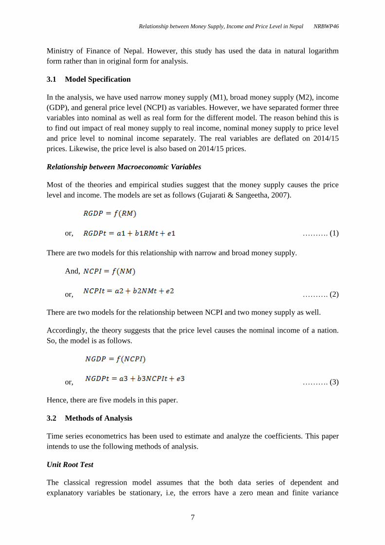
Most of the theories and empirical studies suggest that the money supply causes the price

level and income. The models are set as follows (Gujarati & Sangeetha, 2007).

or, ………. (1)

There are two models for this relationship with narrow and broad money supply.

And,

or, ………. (2)

There are two models for the relationship between NCPI and two money supply as well.

Accordingly, the theory suggests that the price level causes the nominal income of a nation.

So, the model is as follows.

or, ………. (3)

Hence, there are five models in this paper.

3.2 Methods of Analysis

Time series econometrics has been used to estimate and analyze the coefficients. This paper

intends to use the following methods of analysis.

Unit Root Test

The classical regression model assumes that the both data series of dependent and

explanatory variables be stationary, i.e, the errors have a zero mean and finite variance


8

(Enders, 2010). But in the most cases, the macroeconomic time series are non-stationary

(Asteriou & Hall, 2007). ‘Whether the data is stationary or not?’ we can find out by

performing the unit root test. There are few methods of testing unit root of the data. Here, the

paper has performed the Augmented Dickey-Fuller (ADF) test for the test of stationarity of

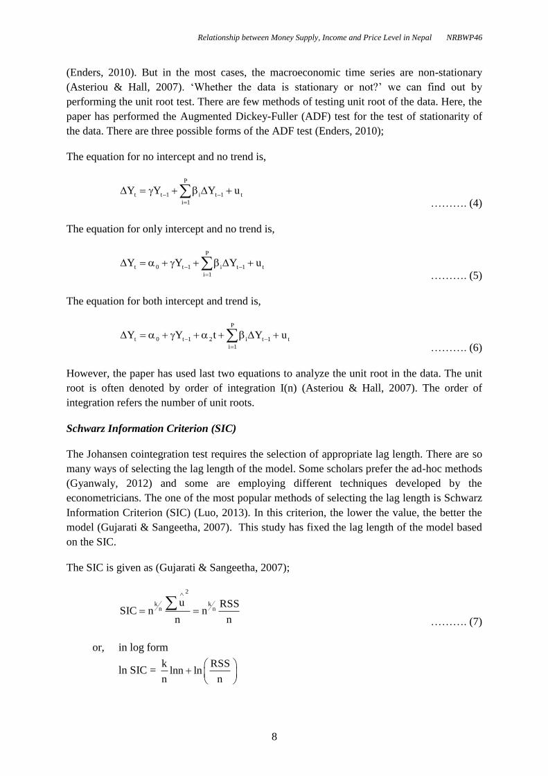
the data. There are three possible forms of the ADF test (Enders, 2010);

The equation for no intercept and no trend is,

P

t t 1 i t 1 t

i 1

Y Y Y u

………. (4)

The equation for only intercept and no trend is,

P

t 0 t 1 i t 1 t

i 1

Y Y Y u

………. (5)

The equation for both intercept and trend is,

P

t 0 t 1 2 i t 1 t

i 1

Y Y t Y u

………. (6)

However, the paper has used last two equations to analyze the unit root in the data. The unit

root is often denoted by order of integration I(n) (Asteriou & Hall, 2007). The order of

integration refers the number of unit roots.

Schwarz Information Criterion (SIC)

The Johansen cointegration test requires the selection of appropriate lag length. There are so

many ways of selecting the lag length of the model. Some scholars prefer the ad-hoc methods

(Gyanwaly, 2012) and some are employing different techniques developed by the

econometricians. The one of the most popular methods of selecting the lag length is Schwarz

Information Criterion (SIC) (Luo, 2013). In this criterion, the lower the value, the better the

model (Gujarati & Sangeetha, 2007). This study has fixed the lag length of the model based

on the SIC.

The SIC is given as (Gujarati & Sangeetha, 2007);

2

k kn n

u RSSSIC n n

n n

………. (7)

or, in log form

ln SIC = k RSS

lnn lnn n


9

Johansen Cointegration Test

The cointegration refers the existence of a long-run equilibrium relationship between the

variables in which an economic system converges over time (Bhusal, 2016). In general, for

the cointegration test, the all data series used in the model should be integrated in same order.

While testing the cointegration one cannot use the first difference data rather should use the

level data. So, cointegration becomes an over-riding need for any econometric modelling

occupying the non-stationary time series (Asteriou & Hall, 2007).

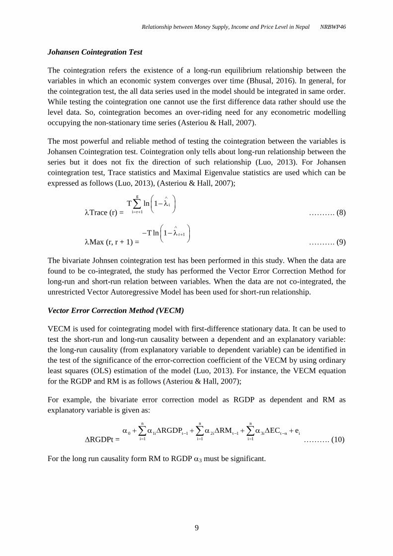
The most powerful and reliable method of testing the cointegration between the variables is

Johansen Cointegration test. Cointegration only tells about long-run relationship between the

series but it does not fix the direction of such relationship (Luo, 2013). For Johansen

cointegration test, Trace statistics and Maximal Eigenvalue statistics are used which can be

expressed as follows (Luo, 2013), (Asteriou & Hall, 2007);

Trace (r) =

g

i

i r 1

T ln 1

………. (8)

Max (r, r + 1) = r 1T ln 1

………. (9)

The bivariate Johnsen cointegration test has been performed in this study. When the data are

found to be co-integrated, the study has performed the Vector Error Correction Method for

long-run and short-run relation between variables. When the data are not co-integrated, the

unrestricted Vector Autoregressive Model has been used for short-run relationship.

Vector Error Correction Method (VECM)

VECM is used for cointegrating model with first-difference stationary data. It can be used to

test the short-run and long-run causality between a dependent and an explanatory variable:

the long-run causality (from explanatory variable to dependent variable) can be identified in

the test of the significance of the error-correction coefficient of the VECM by using ordinary

least squares (OLS) estimation of the model (Luo, 2013). For instance, the VECM equation

for the RGDP and RM is as follows (Asteriou & Hall, 2007);

For example, the bivariate error correction model as RGDP as dependent and RM as

explanatory variable is given as:

RGDPt =

n n n

0 1i t 1 2i t 1 3i t n i

i 1 i 1 i 1

RGDP RM EC e

………. (10)

For the long run causality form RM to RGDP 3 must be significant.


10

Unrestricted Vector Autoregressive (VAR) Model

The models which are not co-integrated has been tested short run causality under unrestricted

VAR. As the data are integrated of first order, the first-difference data have been used for the

VAR models. The equation of bivariate VAR models are as follows (Asteriou & Hall, 2007);

ΔRGDPt = 10 – 12 ΔRMt + 11 ΔRGDPt–1 + 12 ΔRMt–1 + uyt ………. (11)

ΔRMt = 20 – 21 ΔRGDPt + 21 ΔRGDPt–1 + 22 ΔRMt–1 + uxt ………. (12)

Granger Causality Test

The Granger causality/ block exogeneity Wald test has been performed under both VECM

and VAR for the short-run causality between the variables. For instance, the Granger

causality test between real income and real money supply is given as (Gujarati & Sangeetha,

2007);

………. (13)

………. (14)

Where e2t and e3t are disturbances and assumed to be uncorrelated to each other.

Unidirectional causality from RM to RI is indicated if Σbi≠0 and Σhi=0. Conversely,

unidirectional causality from RI to RM exists if Σbi=0 and Σhi≠0. Feedback or bilateral

causality is suggested if both coefficients Σbi≠0 and Σhi≠0. Finally, independence is

suggested if Σbi=0 and Σhi=0. (Gujarati & Sangeetha, 2007).

The Granger causality test for other models are also same as above.

Residual Test

The serial correlation is tested by using Breush- Godfrey Serial Correlation LM tests in this

study. The heteroscedasticity is checked by using Breush-Pagan Godfrey test. Accordingly,

Jarque-Bera test is used to test the normality of residuals. Similarly, Cumulative Sum test and

cumulative sum of square test are used to test the stability of the models.

IV. EMPIRICAL ANALYSIS

4.1 Results of Unit Root Test

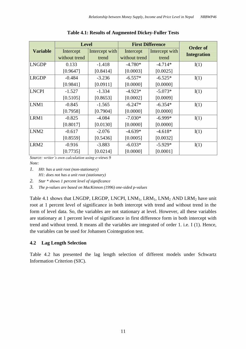
The Augmented Dickey-Fuller (ADF) is used to test the unit root of the dependent and

explanatory variables. Table 4.1 shows the results of Augmented Dickey-Fuller tests of the

time series variables used in this study.


11

Table 4.1: Results of Augmented Dickey-Fuller Tests

Variable

Level First Difference Order of

Integration Intercept

without trend

Intercept with

trend

Intercept

without trend

Intercept with

trend

LNGDP 0.133

[0.9647]

-1.418

[0.8414]

-4.780*

[0.0003]

-4.714*

[0.0025]

I(1)

LRGDP -0.484

[0.9841]

-3.236

[0.0911]

-6.557*

[0.0000]

-6.525*

[0.0000]

I(1)

LNCPI -1.527

[0.5105]

-1.334

[0.8653]

-4.923*

[0.0002]

-5.073*

[0.0009]

I(1)

LNM1 -0.845

[0.7958]

-1.565

[0.7904]

-6.247*

[0.0000]

-6.354*

[0.0000]

I(1)

LRM1 -0.825

[0.8017]

-4.084

[0.0130]

-7.030*

[0.0000]

-6.999*

[0.0000]

I(1)

LNM2 -0.617

[0.8559]

-2.076

[0.5436]

-4.639*

[0.0005]

-4.618*

[0.0032]

I(1)

LRM2 -0.916

[0.7735]

-3.883

[0.0214]

-6.033*

[0.0000]

-5.929*

[0.0001]

I(1)

Source: writer’s own calculation using e-views 9

Note:

1. H0: has a unit root (non-stationary)

H1: does not has a unit root (stationary)

2. Star * shows 1 percent level of significance

3. The p-values are based on MacKinnon (1996) one-sided p-values

Table 4.1 shows that LNGDP, LRGDP, LNCPI, LNM1, LRM1, LNM2 AND LRM2 have unit

root at 1 percent level of significance in both intercept with trend and without trend in the

form of level data. So, the variables are not stationary at level. However, all these variables

are stationary at 1 percent level of significance in first difference form in both intercept with

trend and without trend. It means all the variables are integrated of order 1. i.e. I (1). Hence,

the variables can be used for Johansen Cointegration test.

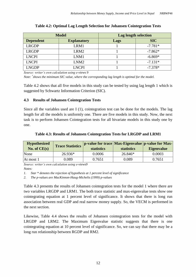
4.2 Lag Length Selection

Table 4.2 has presented the lag length selection of different models under Schwartz

Information Criterion (SIC).


12

Table 4.2: Optimal Lag Length Selection for Johansen Cointegration Tests

Model Lag length selection

Dependent Explanatory Lags SIC

LRGDP LRM1 1 -7.781*

LRGDP LRM2 1 -7.862*

LNCPI LNM1 1 -6.869*

LNCPI LNM2 1 -7.131*

LNGDP LNCPI 1 -7.378*

Source: writer’s own calculation using e-views 9

Note: *shows the minimum SIC value, where the corresponding lag length is optimal for the model.

Table 4.2 shows that all five models in this study can be tested by using lag length 1 which is

suggested by Schwartz Information Criterion (SIC).

4.3 Results of Johansen Cointegration Tests

Since all the variables used are I (1), cointegration test can be done for the models. The lag

length for all the models is uniformly one. There are five models in this study. Now, the next

task is to perform Johansen Cointegration tests for all bivariate models in this study one by

one.

Table 4.3: Results of Johansen Cointegration Tests for LRGDP and LRM1

Hypothesized

No. of CE(s) Trace Statistics

p-value for trace

statistics

Max-Eigenvalue

statistics

p-value for Max-

Eigenvalue

None 26.936* 0.0006 26.846*

0.0003

At most 1 0.089

0.7651 0.089

0.7651

Source: writer’s own calculation using e-views9

Notes:

1. Star * denotes the rejection of hypothesis at 1 percent level of significance

2. The p-values are MacKinnon-Haug-Michelis (1999) p-values

Table 4.3 presents the results of Johansen cointegration tests for the model 1 where there are

two variables LRGDP and LRM1. The both trace statistic and max-eigenvalue tests show one

cointegrating equation at 1 percent level of significance. It shows that there is long run

association between real GDP and real narrow money supply. So, the VECM is performed in

the next section.

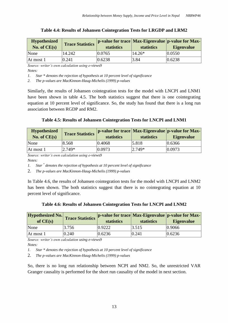
Likewise, Table 4.4 shows the results of Johansen cointegration tests for the model with

LRGDP and LRM2. The Maximum Eigenvalue statistic suggests that there is one

cointegrating equation at 10 percent level of significance. So, we can say that there may be a

long run relationship between RGDP and RM2.


13

Table 4.4: Results of Johansen Cointegration Tests for LRGDP and LRM2

Hypothesized


p-value for trace

statistics

Max-Eigenvalue

statistics

p-value for Max-

Eigenvalue

None 14.242

0.0765 14.26*

0.0550

At most 1 0.241

0.6238 3.84

0.6238


Notes:



Similarly, the results of Johansen cointegration tests for the model with LNCPI and LNM1

have been shown in table 4.5. The both statistics suggest that there is one cointegrating

equation at 10 percent level of significance. So, the study has found that there is a long run

association between RGDP and RM2.

Table 4.5: Results of Johansen Cointegration Tests for LNCPI and LNM1

Hypothesized


p-value for trace

statistics

Max-Eigenvalue

statistics

p-value for Max-

Eigenvalue

None 8.568

0.4068 5.818

0.6366

At most 1 2.749*

0.0973 2.749*

0.0973


Notes:



In Table 4.6, the results of Johansen cointegration tests for the model with LNCPI and LNM2

has been shown. The both statistics suggest that there is no cointegrating equation at 10

percent level of significance.

Table 4.6: Results of Johansen Cointegration Tests for LNCPI and LNM2

Hypothesized No.

of CE(s) Trace Statistics

p-value for trace

statistics

Max-Eigenvalue

statistics

p-value for Max-

Eigenvalue

None 3.756 0.9222 3.515

0.9066

At most 1 0.240 0.6236 0.241 0.6236


Notes:



So, there is no long run relationship between NCPI and NM2. So, the unrestricted VAR

Granger causality is performed for the short run causality of the model in next section.


14

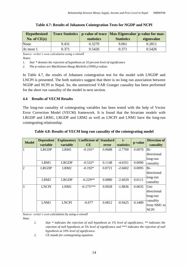
Table 4.7: Results of Johansen Cointegration Tests for NGDP and NCPI

Hypothesized

No. of CE(s)

Trace Statistics p-value of trace

statistics

Max-Eigenvalue

Statistics

p-value for max-

eigenvalue

None 9.431 0.3270 9.061 0.2811

At most 1 0.371 0.5426 0.371 0.5426


Notes:



In Table 4.7, the results of Johansen cointegration test for the model with LNGDP and

LNCPI is presented. The both statistics suggest that there is no long run association between

NGDP and NCPI in Nepal. So, the unrestricted VAR Granger causality has been performed

for the short run causality of the model in next section.

4.4 Results of VECM Results

The long-run causality of cointegrating variables has been tested with the help of Vector

Error Correction Model (VECM) framework. It is found that the bivariate models with

LRGDP and LRM1, LRGDP and LRM2 as well as LNCPI and LNM1 have the long-run

cointegrating relationship.

Table 4.8: Results of VECM long run causality of the cointegrating model

Model Dependent

variable

Explanatory

variable

Coefficient of

CE

Standard

error

t-

statistics p-value

Direction of

causality

1 LRGDP LRM1 -0.191* 0.0688 -2.7700 0.0070 Bi-

directional

long-run

causality LRM1 LRGDP -0.532* 0.1148 -4.6351 0.0000

2 LRGDP LRM2 -0.192* 0.0721 -2.6602 0.0095 Bi-

directional

long-run

causality LRM2 LRGDP -0.229** 0.0880 -2.6029 0.0111

3 LNCPI LNM1 -0.175*** 0.0928 -1.8836 0.0635 Uni-

directional

long-run

causality

from NM1 to

NCPI

LNM1 LNCPI -0.077 0.0812 -0.9425 0.3489

Source: writer’s own calculation by using e-views9

Note:

1. Star * indicates the rejection of null hypothesis at 1% level of significance, ** indicates the

rejection of null hypothesis at 5% level of significance and *** indicates the rejection of null

hypothesis at 10% level of significance.

2. CE stands for cointegrating equation.


15

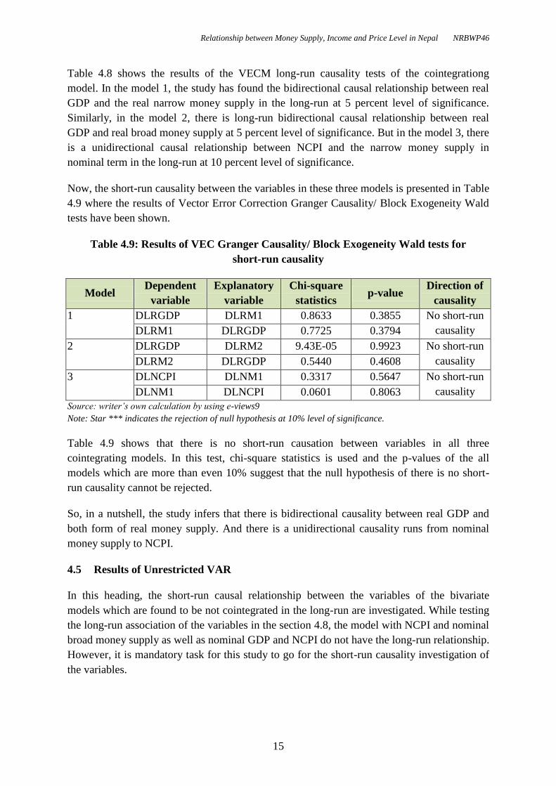
Table 4.8 shows the results of the VECM long-run causality tests of the cointegrationg

model. In the model 1, the study has found the bidirectional causal relationship between real

GDP and the real narrow money supply in the long-run at 5 percent level of significance.

Similarly, in the model 2, there is long-run bidirectional causal relationship between real

GDP and real broad money supply at 5 percent level of significance. But in the model 3, there

is a unidirectional causal relationship between NCPI and the narrow money supply in

nominal term in the long-run at 10 percent level of significance.

Now, the short-run causality between the variables in these three models is presented in Table

4.9 where the results of Vector Error Correction Granger Causality/ Block Exogeneity Wald

tests have been shown.

Table 4.9: Results of VEC Granger Causality/ Block Exogeneity Wald tests for

short-run causality

Model Dependent

variable

Explanatory

variable

Chi-square

statistics p-value

Direction of

causality

1 DLRGDP DLRM1 0.8633 0.3855 No short-run

causality DLRM1 DLRGDP 0.7725 0.3794

2 DLRGDP DLRM2 9.43E-05 0.9923 No short-run

causality DLRM2 DLRGDP 0.5440 0.4608

3 DLNCPI DLNM1 0.3317 0.5647 No short-run

causality DLNM1 DLNCPI 0.0601 0.8063


Note: Star *** indicates the rejection of null hypothesis at 10% level of significance.

Table 4.9 shows that there is no short-run causation between variables in all three

cointegrating models. In this test, chi-square statistics is used and the p-values of the all

models which are more than even 10% suggest that the null hypothesis of there is no short-

run causality cannot be rejected.

So, in a nutshell, the study infers that there is bidirectional causality between real GDP and

both form of real money supply. And there is a unidirectional causality runs from nominal

money supply to NCPI.

4.5 Results of Unrestricted VAR

In this heading, the short-run causal relationship between the variables of the bivariate

models which are found to be not cointegrated in the long-run are investigated. While testing

the long-run association of the variables in the section 4.8, the model with NCPI and nominal

broad money supply as well as nominal GDP and NCPI do not have the long-run relationship.

However, it is mandatory task for this study to go for the short-run causality investigation of

the variables.


16

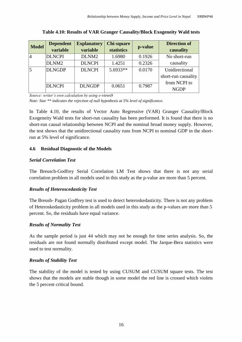
Table 4.10: Results of VAR Granger Causality/Block Exogeneity Wald tests

Model Dependent

variable

Explanatory

variable

Chi-square

statistics p-value

Direction of

causality

4 DLNCPI DLNM2 1.6980 0.1926 No short-run

causality DLNM2 DLNCPI 1.4251 0.2326

5 DLNGDP DLNCPI 5.6933** 0.0170 Unidirectional

short-run causality

from NCPI to

NGDP DLNCPI DLNGDP 0.0651 0.7987


Note: Star ** indicates the rejection of null hypothesis at 5% level of significance.

In Table 4.10, the results of Vector Auto Regressive (VAR) Granger Causality/Block

Exogeneity Wald tests for short-run causality has been performed. It is found that there is no

short-run causal relationship between NCPI and the nominal broad money supply. However,

the test shows that the unidirectional causality runs from NCPI to nominal GDP in the short-

run at 5% level of significance.

4.6 Residual Diagnostic of the Models

Serial Correlation Test

The Breusch-Godfrey Serial Correlation LM Test shows that there is not any serial

correlation problem in all models used in this study as the p-value are more than 5 percent.

Results of Heteroscedasticity Test

The Breush- Pagan Godfrey test is used to detect heteroskedasticity. There is not any problem

of Heteroskedasticity problem in all models used in this study as the p-values are more than 5

percent. So, the residuals have equal variance.

Results of Normality Test

As the sample period is just 44 which may not be enough for time series analysis. So, the

residuals are not found normally distributed except model. The Jarque-Bera statistics were

used to test normality.

Results of Stability Test

The stability of the model is tested by using CUSUM and CUSUM square tests. The test

shows that the models are stable though in some model the red line is crossed which violets

the 5 percent critical bound.


17

V. CONCLUSIONS AND RECOMMENDATIONS

At the end, the paper has found out some conclusions or inferences from the study. The paper

found that there is bidirectional long-run casualty between the real income and real narrow

money supply as well as the real income and real broad money supply. So, it is to conclude

that in the long-run the real money supply causes the real income and real income also

reciprocates the real money supply (without causing in the short-run) in Nepal. In other

words, the money supply causes the income in the long-run with strong feedback effect. But

there is no evidence of short run causation between these two variables. It means the growth

rate of money supply and income in Nepal is not associated.

Likewise, the study has found the unidirectional long-run relationship runs from narrow

money supply to consumer price. However, there is no short-run relationship from either side.

Here, it is to conclude that, the nominal narrow money supply causes the general price level

of the country in the long-run without feedback.

However, there is no evidence of long-run as well as short-run relationship between broad

money supply and consumer price level. It concludes that there is no association between

broad money supply and general price level of Nepal in both short and long run.

From the both short-run results between money supply and inflation, it can be inferred that

there is no evidence of short-run causal relationship between the growth rate of money supply

and inflation in Nepal.

Accordingly, there is no evidence of long-run causality between nominal GDP and general

price level. But the study found the unidirectional short-run causality running from general

price to nominal GDP. It means that the growth rate of general price level affects the growth

rate of nominal income of the nation.

The conclusions of our study do not support the monetarists’ point of view which suggests

that there is causal relationship runs from money supply to income and price in the short-run.

They also postulate that the causality disappears in the long-run. Contrary to that our

conclusion in the Nepalese context suggests that the money supply causes to national income

with the same feedback and causes to price level without feedback in the long-run.

This study also denied the early Keynesians’ ignorance to the important role of money supply

in the economy. However, this study supports the Keynesian view of indirect (long-run)

relationship between the money supply, real income and prices. So, the conclusion of this

study suggests that the money supply has significant role in the long-run rather than short-

run for Nepalese economy.

This study intends to make some inferences which may be useful for the policymaker to

make the appropriate policies for the nation. The major recommendations of this study can be

prescribed as follows;


18

The inflationary pressure in Nepal is so high. As this study suggests, the nominal

narrow money supply causes the general price level in the long-run but broad money

supply does not. So, the monetary policy should be focused to increase the time

deposit rather than the currency and demand deposit in the economy.

In this study, it is found that both real money supply causes the real income of the

nation and real income also causes the both real money supply in the long-run. So,

this paper suggests that the policymakers have to maintain an appropriate growth rate

of money supply in real term to achieve the certain level of real income growth.

On the one hand, the main cause of the growth of nominal income of Nepal is growth

rate of the general price level. On the other hand, the nominal narrow money causes

the price level in the long-run. It means that the policymakers can infer that the

nominal narrow money supply causes the nominal income of the nation indirectly.

Hence, the narrow money supply can be an instrumental to handle the inflation and

nominal growth rate in the long-run.

From the results of this study, the policymakers can view that the broad money supply

is more appropriate than the narrow money supply because both causes the real

income in the long-run but narrow money causes inflation as well. So, the increment

in broad money supply (time deposit component) is healthier than narrow money

supply (currency and demand deposit components) for the Nepalese economy.


19

REFERENCES

Ackley, G. 2007. Macroeconomic Theory (first Indian reprint ed.). Delhi: Surjeet

Publications.

Ahmad, N., Asad, I., & Hussian, Z. 2008. "Money, Prices, Income and Causality: A case

study of Pakistan." The Journal of Commerce 4(4).

Al-Jarrah, M. 1996. "Money, Income and prices in Saudi Arabia : a cointegration and

causality analysis." Pakistan Economic and Social Review 34(1): 41-53.

Asteriou, D., & Hall, S. G. 2007. Applied Econometrics (first revised ed.). New York:

Palgrave Macmillan.

Bhusal, T. P. 2016. Basic Econometrics (revised ed.). Kathmandu: Dreamland Publication (P)

Ltd.

Blinder, A. S. 1988. "The fall and Rise of Keynesian Economics." Economic Record, 278-

294.

Branson, W. H. 2005. Macroeconomic Theory and Policy (first East-West press ed.). New

Delhi: East-West Press.

Coddington, A. 1976. "Keynesian Economics: The Search for First Principle." Journal of

Economic literature: 1258-73.

Current Macroeconomic and Financial Situation. 2018. Nepal Rastra Bank.

Economic Survey. n.d. (various issues). Ministry of Finance, Government of Nepal.

Enders, W. 2010. Applied Econometric Time Series (third ed.). New Jersey: willy.

Friedman, M., & Schwartz, A. 1963. A Monetary History of the United States 1867-1960.

Princeton Univercity Press.

Froyen, R. T. 2014. Macroeconomics, Theories and Policies (tenth ed.). Noida: Pearson India

Education Services.

Gordon, R. J. 1990. "What is New-Keynesian Economics?" Journal of Economic Literature.

Gujarati, D. N., & Sangeetha. 2007. Basic Econometrics (fourth ed.). New Delhi: The

McGraw-Hill Companies.

Gyanwaly, R. P. 2012. "Causal Relationship between Money, Price and Incme in Asian

countries (1964-2011)." The Economic Journal of Nepal 35(1): 12-31.

Holod, D. 2000. "The Relationship between Price Level, Money Supply and Exchange Rate

in Ukraine." National University of Kiev-Mohyla Academy.

Ihsan, I., & Anjum, S. 2013. "Impact of Money Supply (M2) on GDP of Pakistan." Global

Journal of Management and Business Research Finance 13(6).

Intelligent Economist. n.d.. Retrieved from www.intelligenteconomist.com.

Khatiwada, Y. R. 1994. "Some Aspects of Monetary Policy in Nepal." New Delhi: South

Asian Publishers.


20

Koti, C. S., & Bixho, T. 2016. "Theories of Money Supply: The Relationship of Money

Supply in a Period of Time T-1 and Inflation in Period T- Empirical Evidence from

Albania." European Journal of Multidisciplinary Studies 1(1).

Laidler, D. 1981. "Monetarism: an Interpretation and an Assessment." Economic Journal, 1-

28.

Luo, P. 2013. "Money supply behaviour in 'BRICS' economies." Jonkoping University.

Maddock, R., & Carter, M. 1982. "A Child Guide to Rational Expectations." Journal of

Economic Literature, 39-51.

Mayer, T. 1975. "The Structure of Monetarism." Kredit and Kapital.

NRB. 2001. "Money and Price Relationship in Nepal: A Revisit." Economic Review:

Occasional Paper 13(1): 50-65.

Quarterly Economic Bulletin. 2017. Nepal Rastra Bank.

Salih, M. A. 2013. "Money, Income and Prices in Saudi Arabia." Global Journal of

Management and Business research 13(1): 33-42.

Shapiro, E. 2001. Macroeconomic Analysis (fifth ed.). New Delhi: Galgotia Publications Pvt.

Ltd.

Sims, C. G. 1972. Money, Income and Causality. The American Economic Review 62(4):

540-552.

Singh, C., Das, R., & Baig, J. 2015. "Money, Output and Prices in India." IIMB- Working

Paper 497.

Documents

Relationship between Money Supply, Income and Price Level