Student

Umeå School of Business

Spring semester 2010 Master thesis, one-year,15 hp

RELATIONSHIP BETWEEN THE

PROFITABILITY AND WORKING

CAPITAL POLICY OF SWEDISH

COMPANIES

Authors: Wajahat Ali Syed Hammad Ul Hassan

Supervisor: Catherine Lions

I

Acknowledgement First of all we are thankful to ALLAH the ALMIGHTY, the most beneficial and merciful

who gave us the courage to finish our thesis

Secondly, we wish to express our gratitude to our supervisor Prof. Catherine Lion for

her constructive advice, directions, comments, support and professional guidance. We are

also thankful to Prof. Anders Muszta (Department of statistics, Umea University) and

Prof Pryanka (Department of statistics, Umea University) for their help to acquire an in-

depth knowledge of the statistics and SPSS. We are also extremely thankful to all the

authors of the references in our thesis.

Finally, the prayers from our families played an important role in the completion of the

thesis. Without their moral and financial support it would have been impossible for us to

write this thesis report.

_____________________ Syed Hammad ul Hassan Student, Umea University Hamad381@gmail.com ____________________ Wajahat Ali Student, Umea University Wajahat_ali_bajwa@yahoo.com

II

Abstract Over the years there has been a big debate on the effect of working capital policy on the profitability. Few researchers argue that working capital is just an idle resource with a high cost and low benefit associated with it so, companies should follow zero working capital policy but such a policy is very risky because it reduces the liquidity and it might leads to a default. Other researchers support companies to have a working capital policy because they believe that proper management of components of working capital can balance cost and benefits of the company and it will reduce the risk of default by raising the level of liquidity. Companies can choose among three different types of working capital i.e. aggressive, conservative and moderate but their choice depends on their desire level of liquidity and risk. Researchers realize the importance of the topic and lot of research has been carried out all over the world especially in developing countries like Pakistan, India, and Taiwan etc. Despite the importance of topic we were unable to find any research carried out in Sweden or in any other Scandinavian country. So, this study is conducted with the purpose to explore the relationship between working capital policy and profitability of Swedish firms. Furthermore this study also investigates the nature of relationship between working capital policy and component of cash conversion cycle. For the purpose of our study we used the sample of 37 listed companies in the OMX Stockholm stock exchange over the period of five years (2004-2008). The study has been conducted in a natural environment and it follows the explanatory research strategy. Moreover it is a quantitative study which follows the deductive approach and it is longitudinal in nature. We used GOP as a measure to profitability and CCC is used as a gauge to measure the aggressiveness of working capital policy. We used the secondary data, which has been extracted from the annual financial reports of the companies, to calculate the GOP, financial debt, firm size, fixed financial asset, component of CCC and CCC. In this study, six regressions were run on 185 observations in SPSS software. In each regression analysis dependent variable (GOP), independent variable firm size, financial debt ratio, and fixed financial asset ratio remains the same but independent variable CCCS, CCCA, CCCD, day’s inventory held, days account receivable and days account payable replace each other. The reason for this replacement of independent variables is to find out that how CCC and component of CCC affects the GOP. The result of regression analysis shows that managers can’t change the level of profitability by adopting any of the working capital policy i.e. there exist no relationship between working capital policy and profitability. Furthermore profitability is directly associated with days inventory held and days account payable but it is in inverse relation with days account receivables.

III

Table of Contents

1. Introduction 1 1.1 Choice of a topic 1 1.2 Background 2 1.3 Purpose of the study 4 1.4 Research question 4 1.5 Limitations 4 1.5.1 Language limitations 4 1.5.2 Research limitations 4 1.5.3 Data limitations 5 1.6 Definitions 5 1.6.1 Gross working capital policy 5 1.6.2 Net working capital policy 5 1.6.3 Liquidity 5 1.7 Disposition 6 2. Methodology 7 2.1 Statement of the problem 7 2.2 Scope of the study 7 2.3 Research philosophy 7 2.3.1 Positivism 8 2.3.2 Phenomenology 8 2.4 Research approach 8 2.4.1 Deductive Approach 8 2.4.2 Inductive Approach 8 2.5 Research methods 9 2.5.1 Quantitative method 9 2.5.2 Qualitative method 9 2.6 Research design 9 2.7 Research criteria 9 2.8 Research Credibility 10 2.8.1 Reliability 10 2.8.2 Validity 10 2.8.3 Generalization 10 2.9 Data Collection and Sample 10 3. Theoretical Framework 13 3.1 Conceptual Framework 13 3.1.1 Net Working capital 13 3.1.1.1 Current Assets 14 3.1.1.1.1 Account Receivable 14 3.1.1.1.2 Inventory 15 3.1.1.1.3 Short term Investments 16 3.1.1.1.4 Cash 16 3.1.1.2 Current Liabilities 18

IV

3.1.1.2.1 Account Payables 18 3.1.1.2.2 Short term Borrowings 18 3.1.2 Importance of working capital management 19 3.1.3 Working Capital Policy 19 3.1.4 Cash Conversion Cycle 21 3.1.4.1Components of CCC 21 3.1.4.1.1 Collection period or Days account receivable 21 3.1.4.1.2 Day’s inventory held 22 3.1.4.1.3 Days Account payables 22 3.1.5 Profitability 22 3.1.5.1 Profitability Ratios 23 3.1.5.1.1 Return on Equity 23 3.1.5.1.2 Net Profit Margin 23 3.1.5.1.3Return on Total Asset 23 3.1.5.1.4 Gross operation profit 23 3.1.6 Liquidity versus Profitability 24 3.1.7 Financial Assets 24 3.1.8 Financial Debt 25 3.2 WC Practice in different geographical areas 25 3.2.1 WC practice in Developing Asian countries 25 3.2.2 WC practice in European Companies 26 3.2.3 WC practice in US 27 3.2.4 Empirical studies in Scandinavia 28 4. Results and Analysis 29 4.1 Variables 29 4.1.1 Independent Variable 29 4.1.2 Dependent Variable 30 4.2 Hypothesis 30 4.2.1 Hypothesis 1 31 4.2.2 Hypothesis 2 31 4.2.3 Hypothesis 3 32 4.2.4 Hypothesis 4 32 4.2.5 Hypothesis 5 32 4.2.6 Hypothesis 6 33 4.3 Fundamental Concepts for Analysis 33 4.3.1 F value 33 4.3.2 T Value 33 4.3.3 R Square 33 4.3.4 P Value 34 4.3.5 95 % Confidence Interval 34 4.3.6 Durbin Watson Test 34 4.3.7 Correlation 34 4.3.8 Beta 34 4.4 Descriptive Statistics 35 4.5 Correlation 35 4.6 Regression Analysis 38

V

4.6.1 Regression 1 39 4.6.2 Regression 2 40 4.6.3 Regression 3 41 4.6.4 Regression 4 42 4.6.5 Regression 5 43 4.6.6 Regression 6 44 4.7 Discussion 46 5. Credibility Criteria 47 5.1 Reliability 47 5.2 Validity 47 5.3 Generalization 47 6. Further Research 48 7. Conclusion 49 8. References 51 9. Glossary 53 10. Appendix 54

1

1. Introduction This chapter is an introductory part of our research and it includes some major aspects which are necessary to understand for the later part of the study. The reader of this part will find the information about the Choice of topic, Background of the study, Purpose of a study, Research question for which this study is conducted, Limitations , Definitions of the terms and Disposition of the report. 1.1 Choice of a topic Investors all over the world put their money in a business to get some return on their investment in any form of the business (proprietorship, partnership and corporations). In small and medium businesses like proprietorship and partnership owners have direct or indirect control over the management of the business so, they themselves are responsible for all the profit and loss. On the other hand in the large multinational companies the management of the company manages the affairs of the company on behalf of owners but owners want management to take such decisions which will give positive signal to market, increase the value of the firm, enhance profitability and maximize holding period return. The heart of corporate finance literature is long term investment, capital structure and different valuation methods. They have been focus of intention for many researchers in the past. In short it is mainly concern with the long term financial planning or decisions. On the other hand it is believed that financial decisions of short term assets and short term liabilities management also influence the stock price. These financial decisions are vital because they demonstrate the financial stability of the firm and market develops perception about the firm accordingly (Afza & Nazir, 2008). In order to find new ways of value creation, most of the empirical studies focused on inventory management and account receivables management but working capital management has a broader view. It not only covers the current assets but also covers the current liabilities (Lazaridis & Tryfonidis, 2006). A proficient policy towards working capital can create value for the shareholders, on the other hand a deprived policy might affect the business in a appalling way and might cause a financial distress. This situation will lead to the disinvestment and failure of all the long terms plan resultantly shareholder will loose the value (Afza & Nazir, 2008). The importance of working capital policy or management can’t be denied in any organization. Researchers all over the world focused on this issue and discuss it in detail in the perspective of many countries. Researchers from developing countries consider working capital as a life blood of any organization and this is the reason that most of the research on the topic had been carried out in the developing countries e.g. Pakistan, India, and Taiwan etc. As we belong to a country where researchers consider the working capital as the most important factor that determine the profitability, it was surprising for us to know that despite the importance of the topic very little research has been carried out in Sweden for an international user i.e. research in English. By keeping this thing in

2

our mind we will focus on the Swedish companies and will try to find out the association between profitability and working capital policy. 1.2 Background The ploy, plan or tactic which gives the road map to manage the short term assets and short term liabilities in such a way that it reduces the risk of default is known as working capital policy or it is a strategy to manage the difference between the current asset and current liabilities (Brian, 2009). The literature of finance classifies working capital policy into three categories (Brian, 2009).

• Aggressive policy • Defensive policy • Conservative policy

Current assets are most important component of working capital as the policy which a company adopts towards working capital also depends on the level of current assets. Aggressive policy can be adopted to create value by maintaining low level of current assets as compared to current liabilities. It will create value but at the same time it will increase the risk of default. On the other hand it can follow the defensive policy by increasing the level of current assets as compared to current liabilities, it will reduce the risk of default but there is an opportunity cost associated with it, which might cause the reduction in profitability (Afza & Nazir, 2008). We have witnessed the change in trend in the management of working capital. Earlier companies preferred to have high level of working capital to meet their financial obligations but with the passage of time, with the introduction of new technology and new ways of managing current assets high level of working capital is considered as a burden on a company. Now the trend has been changed and companies consider the high working capital as an idle resource which doesn’t have any use and it doesn’t create any value for the company. Therefore, companies prefer to have no working capital policy but want to have enough cash in hand to meet current financial obligations. The central point or the focus of working capital policy is on the liquidity of current assets to meat the short term or current liabilities. Liquidity gives the true idea of firm’s position to meet its maturing liabilities. A firm should have sufficient level of liquidity because excessive liquidity results into idle funds which do not create any value. On the other hand low level of liquidity might result into the lack of resources to meet financial obligations hence creates financial distress (Vishnani & Shah 2007).So we can define working capital policy as a policy, which creates a breakeven of cash flow i.e. same level of cash inflow and cash outflow. Such a cash flow will help to manage the affairs of business in an efficient way (Brian, 2009), but it is not a simple concept to establish such policy without proper understanding of the drivers of working capital. It emerges as a major problem in the organizations where finance department is unable to identify the basic drivers and appropriate level of working capital. A good understanding of these drivers and their role helps the finance managers to reduce the risk of default and to boost up the performance (Lamberson, 1995). An effective management of receivables,

3

payables and inventory contributes a major part of success in any business. All these things are components of working capital and poor management of these components might leads to a failure of business activities. A large number of firms have a large investment in current assets like account receivables and inventories. A survey by national bank of Belgium shows that all the non financial business in Belgium has 17% of total assets is invested in account receivables and 13% in inventories and together they are 30% of total asset which is a large percentage. These figures don’t show the true value of current asset because there are lots of other kinds of current assets in which a company can invest. Keeping this fact in mind one can easily judge that the total current assets of non financial firms are from 30% to 40% of total assets, which really shows the importance of working capital management (Deloof, 2003). Most firms have defined their optimal level of working capital, which will create value for them. For such firms working capital is a part of their financial management strategy. For instance in order to increase their sales different firms uses different credit policies. Strict credit policy will result in the decrease in the sale therefore companies prefer to have such a policy which facilitates the customers and the objectives of the firm. Furthermore such a credit is inexpensive source of finance for the customers rather than borrowing money from any financial institution thus it increases the sale. This credit sale system needs more investment in the account receivables. Some company offers some kind of discount on early payments, which helps to convert account receivables into cash. On the other hand in order to fulfill high sales company need to have sufficient supply and an optimal level of inventory. Since company has invested some money in the account receivables it prefers to buy raw material on the credit terms which match the credit period of account receivables. By following such credit policies companies can create demand and have sufficient supply to meet the demand, it will increase their profitability, but at the same time the level of current assets and current liabilities will increase. The total investment in working capital will increase which can disturb the balance between cash inflow and cash outflow. So, companies need to have a strategy, which will help them to make the cash conversion cycle efficient. Many researchers use cash conversion cycle as a tool to measure the effectiveness and aggressiveness of working capital policy. Cash conversion cycle is a time span from the disbursement of cash to supplier till the receipt of payment from the customer. Large time span increase the profitability by increasing the level of sale but at the same time it needs larger investment in working capital. The effect of this increased profitability can disappear if the cost of higher investment in working capital surpasses its benefits (Deloof, 2003). Thus, the main objective of working capital policy is to maintain such a level of cash inflow and cash outflow which will create the balance between each component of working capital. Without such a balance it is impossible to move or bring business operation on a right track. Furthermore it required consistent and continuous monitoring of component of working capital in order to achieve such a balance but if finance executives failed to monitor and manage it well then they use most of their time to fetch unfavorable level of short-term assets and liabilities to the favorable or optimal level (Filbeck & Krueger 2005, Lamberson, 1995).

4

1.3 Purpose of the study It seems obvious that working capital policy has some impact on the profitability of the firm and there exist a relationship between working capital policy and profitability of the firm but still diminutive research had conducted to find out this relationship. We have discussed earlier that CCC is a useful measure of degree of aggressiveness of working capital policy. So, the purpose of our study is to find out the relationship between working capital policy and profitability of Swedish firms by using the cash conversion cycle as a tool to measure aggressiveness of working capital policy. We will use data from the year 2004 to year 2008. Furthermore we will try to develop better and practical understanding of the association between working capital policies on the profitability and will try to meet the gap in the academic literature over this issue. 1.4 Research question The literature of finance discusses a lot about different working capital policies but it doesn’t explain the relationship between working capital policy and profitability. So this research will be carried out with the intention to explore this relationship i.e to find out that whether there is a positive, negative or no relationship between working capital policy and profitability. So, base on this thing we have following research question for our study. What is the association between working capital policies and firm’s Profitability? As we discuss earlier that lot of research has been carried out in different parts of the world but we were unable to identify single research, which is available in English for an international user, on this topic in Sweden. So, we will focus on Swedish firms in order to find out the answer of our question.

1.5 Limitations 1.5.1 Language limitations While working on this report the biggest hurdle we faced was the Swedish language. We believe that because of this constraint we were unable to find any research carried out on this topic in Sweden as we cannot read and understand the research work in Swedish. Moreover few companies have their financial reports in Swedish and it was difficult for us to read their reports so we skipped such companies from our sample. Swedish companies also have their websites in Swedish so it was really difficult for us to explore the websites and find the annual reports. 1.5.2 Research limitations This study is conducted to find the relationship between working capital policy and profitability of the firm. There are lots of measures one can choose to measure the profitability of the firm like return on assets gross operating profit, return on capital etc.

5

Similarly there are lots of measures to check the degree of aggressiveness of working capital policy e.g. current ratio, cash conversion cycle etc. Thus it is not possible for us to conduct a research by considering all the measures of the profitability and working capital policy. So, we choose GOP as a measure of profitability and Cash conversion cycle as a measure of degree of aggressiveness of working capital policy to find out the relationship between working capital policy and profitability. Variation of result is possible if we change measures of profitability or measure of degree of aggressiveness of working capital. For us one of the research limitations is the recent global economic crisis. This crisis affects all the business and companies all over the world are fighting a war of their survival. We believed that this economic crisis had not only influence the profitability of the companies but also affected their policy of working capital. As period of this economic crisis is part of our study period it is quite likely that it will influence the results. 1.5.3 Data limitations This study is conducted over the period of five years (2004-2008). Our initial sample was all the listed companies at OMX Stockholm stock exchange except the companies from water, banking and finance, insurance, business services and renting sector because of their specific nature. For our target population we were unable to find the financial reports of all the companies over the study period. In order to get the annual financial reports of the companies we tried to contact the management of the company via email but unfortunately it didn’t work for us. As a result we didn’t have any option left except to eliminate such companies from our population. Similarly we also eliminate those companies which have their financial reports in Swedish. 1.6 Definitions 1.6.1 Gross Working Capital The term gross working capital or working capital refers to short term or current assets such as cash, marketable securities, account receivables and inventories (Brigham & Houston, 2007, p.513). 1.6.2 Net working capital It is a difference between current assets and current liabilities of the company. (Brigham & Houston, 2007, p.513) 1.6.3 Liquidity Liquidity is an ability of a company to convert its assets into cash. In other words it as a ability of a company to raise cash by the sale of current assets in order to meet the maturing liabilities (Morawski, 2008, p.12).

6

1.7 Disposition 2. Methodology This chapter will provide the reader with information about research philosophy research approach and research methods of our study. Moreover it also includes the research criteria, research credibility, research design, and data collection techniques. 3. Theoretical framework In this section we thoroughly study the articles, research papers, books and journals related to our topic. We divide this section in two parts. First part will help the reader to understand different concepts & models related to this research. Second part includes the research work of different researchers on the topic. 4. Analysis This part includes the selection of variables, hypothesis for our research, explanation of the terms which will be used for analysis and the result of analysis which is conducted in SPSS software. This section will provide the answer to our research question. 5. Credibility Criteria This chapter will show the level of validity, reliability and generalization of our research. 6. Further Research This chapter identifies the research opportunities in the future related to the topic. 7. Conclusion This section concludes the report. 8. References 9. Glossary 10. Appendix This section includes all the calculation tables for our variables.

7

2. Methodology

This section includes Statement of problem and Scope of study. Furthermore it will help the reader to understand the Research philosophies, Research approaches, Research design, Research criteria, Research credibility, Research methods and data collection techniques which are used in this study. 2.1 Statement of the problem Working capital policy is an important issue in any organization because without a proper management of working capital components it will be difficult for the organization to run its operations smoothly. Furthermore working capital policy has been major issue especially in developing countries and in order to explain the relationship between working capital policy and profitability different researches had been carried out in different parts of the world especially in developing countries (Pakistan, India, and Taiwan). Despite the importance this issue failed to attract the attention of researchers in the Sweden. Thus, while surfing on internet, browsing through the books and journals we didn’t find any research carried out on this topic in Sweden. So by keeping this thing in our mind our study will try to find out the relationship between working capital policy and profitability of the Swedish firms and will also try to meet the gap between existing literatures. 2.2 Scope of the study Maintaining a high profitability is a goal of all the business entities. Researchers all over the world believe that one way of maintaining the high profitability is an efficient management of working capital. In order to manage working capital a firm should have a defined policy. There are several ways of measuring profitability of the firms like return on equity, return on assets, and return on capital employed etc but in this research we will only use gross operating profit as a measure of profitability because we want to correlate operating profit to operating assets of the firm. Cash conversion cycle will be used to measure the aggressiveness of working capital policy. So, we will find the relationship between GOP & CCC in order to explain the relationship between profitability and working capital policy. This research will be helpful for the companies to understand the importance of working capital policy for the profitability. Students and other researchers will also be benefited by this research because it will explain the current trend in the market. 2.3 Research philosophy There are two views of research philosophy.

8

2.3.1 Positivism Followers of this philosophy work with the observable reality and they work independently e.g. neither they influence the subject nor subject influences them. It focuses on well structured methodology which will lead to statistical analysis (Saunders & lewis,2000, P.84-85). 2.3.2 Phenomenology Followers of this philosophy try to explore the reality behind the situation or in other words they try to find out the reality behind another reality. Thus, in order to understand the reality they study the situation in detail (Saunders & lewis,2000, P.85-86). Among the two philosophies of research positivism really supports our purpose of research because we want to work with observable reality (Relationship between working capital policy and profitability) and we are not going to explore the reality working behind the reality. We will collect data independently (without the influence of anyone) and will analyze it by applying statistical tools. In this situation neither subject will influence us nor will we influence it. 2.4 Research approach The literature of business research categorizes research approaches in two categories. 2.4.1 Deductive Approach It is also known as theory testing approach. In this approach researchers develop hypothesis at the first step then in order to test this hypothesis they develop research strategy. It is considered as a casual approach to define a relationship between two variables. Regardless of the result of the existing researches this approach gives researchers freedom to do their research and present their own findings which might contradict with previous studies (Saunders & lewis,2000, P.87-88). 2.4.2 Inductive Approach It is also known as theory building approach. It is opposite to deductive approach. In this approach researchers collect data at the first stage and then by doing the analysis on this data they develop theory. In other words it explains the reasons for the event rather than explaining the event (Saunders & lewis, 2000, P.88-89). In our study we followed the deductive approach because we will develop the hypothesis at the first stage and than in order to test the hypothesis we will analyze our data. Moreover, deductive approach is also used for explaining the relationship between two variables. This thing also encouraged us to follow this approach because we want to investigate the relationship between two variables.

9

2.5 Research methods There are two methods of conducting a research one is quantitative and other is qualitative. 2.5.1 Quantitative method In this method standardized data or numerical data is collected for the purpose of analysis. The analysis is conducted with the help of statistical tolls e.g. correlation, regression etc. This method is adopted by the researchers when they want to explain the relationship between two variables (Saunders & Lewis, 2000, P.370-381). 2.5.2 Qualitative method The data collected in this method is non-standardized and before the analysis it is classified into different categories. The analysis of this data is conducted by the use of conceptual framework. The data of this method is in the form of words or diagrams (Saunders & Lewis, 2000, P.380-405). Quantitative method is followed in this study because the collected data will be in the form of numerical digits and we will use statistical tools for analysis. We will do regression analysis in SPSS to explain the relationship between working capital policy and firm’s profitability. 2.6 Research design This research will try to explore an issue (relationship between working capital policy and profitability of Swedish firms) which had failed to attract the attention of researchers. So, the research has been designed in a way that it will not only contribute to the existing knowledge but it will also meet the requirement and purpose of the study. It will be a longitudinal study and will follow explanatory research strategy as we want to find out the relationship between working capital policy and profitability over a period of five years (2004-2008). We will use the secondary data, which is quantitative in nature, of the selected companies for the statistical analysis in the SPSS which is consistent with our research strategy (Saunders & Lewis, 2000, P96-98). 2.7 Research criteria This research wants to find out the relationship between two variables which is impossible to explain in an artificial environment. So, it is an explanatory research in nature which will be conducted in a natural environment without any influence. Secondary data is used for this research which is collected from articles, websites, books and financial reports.

10

2.8 Research Credibility We judge the credibility of a research on three bases. 2.8.1 Reliability Reliability explains that the result will be the same even if the research will be carried out by another researcher on a different occasion. Furthermore it should not be subject bias, observer bias and it should not have any subject error (Saunders & Lewis, 2000, P.100-101). 2.8.2 Validity Validity means the findings of a research are real e.g. the research conducted to explain the relationship between two variables will show the same relationship as it is in reality and there exist no fictitious numbers or values to make the results attractive (Saunders & Lewis, 2000, P.101-102). 2.8.3 Generalization It is also known as external validity. It explains that to which extent the results of your research are applicable to other research settings. If the research is not conducted with the intention to find or develop a theory which can be generalized then one could explain that what is actually happening in your research settings (Saunders & lewis, 2000, P102-103). In this research we will collect the data from the audited financial reports of listed companies and then we will run statistical analysis on this data. This data belongs to real world and the values of different accounts (Assets, sale, COGS, account receivable, inventory etc) in audited financial reports of previous years can’t be fictitious and can’t be changed. So, the relationship that we will find in this research will be real (Validity), applicable to other research settings (Generalization) and will yield same results even if the research will be carried out by someone else (Reliability). 2.9 Data Collection and Sample For the purpose of our research we choose listed companies at OMX Stockholm stock exchange. In order to make our research more diverse we choose the companies from five different sectors (Industrial sector, It sector, Telecommunication, material and consumer discretionary) and doesn’t include the companies from water, banking and finance, insurance and renting sector because of their specific nature. We concentrate only on listed companies because of the reliability and accuracy of data provided by them in their annual reports. Companies listed at stock exchange want to create the value for shareholders so, they are expected to present the true picture of their income, expenses, assets and liabilities, the accuracy of these accounts can affect the significance of the result of the study. Furthermore for listed companies there is a requirement to conduct

11

external audit which ensures the precision of financial statements. On the other hand non listed firms used different ploy to avoid tax and getting new loan. Hiding of profit and liability and showing more book value of assets is common practice. Inclusion of such companies has a big risk for the purpose of research because result will not show the true picture of actual practice of working capital and its relation with the profitability. In order to make our research more comprehensive we select the population of 93 companies from five different sectors (Consumer discretionary, Material, Telecommunication, IT sector and industrial sector) over the period of 2004-2008. For the selection of our sample we followed convenient sampling technique because it allows the researcher to set a standard for the selection of sample and choose the sample according to his convenience (Malhotra, 2004, p.321). Thus we set availability of financial reports over the period of study as a standard for the selection of a company for a sample. We collect the financial reports of the companies from their websites (web address of these companies was obtained from the website of OMX Stockholm stock exchange) but unfortunately the financial statements for some companies were missing over the period of study. So, we exclude such companies from our original sample and left with the final sample of 37 companies and with 185 total observations. Following companies are part of the sample: 1. ABB ltd 2. Alfa Laval corporate AB 3. Assa Abloy 4. Atlas copco 5. Beijer AB 6.DFDS 7. DS Norden 8. FLSmidth 9.Gunnebo 10. ITAB 11. konecranes 12.Emminkainen 13. Lindab 14. Marel hf 15.Metso 16. Sanistaal 17. Scania 18. Securitas AB 19. Systemair 20.Vacon 21.Xano 22. YIT 23. Anoto 24.Ericson 25. Lbi 26. Nokia 27.Note AB 28. Tele 2 29. Novozymes 30.Outokumpu 31. SCA 32. Saab AB 33.Bang & Olufsen 34. Electrolux 35.Eniro 36.Nobia 37.Rapalaworld For the in-depth study of the topic we have decided to split our sample in two sub groups based on the aggressiveness of working capital policy.

• Observations with aggressive working capital policy • Observations with defensive working capital policy

These subgroups will help us to understand the actual relationship between WCP and profitability because in our subgroups we will study the homogeneous observations and not the companies. There is fair chance that result of analysis for these subgroups contradicts the result of analysis for the sample. Moreover, the results will help us to check the validity and authenticity of debate in the literature about the association of WCP and profitability. This will be a unique effort, as none of the previous studies

12

divided their sample into subgroups to find out the association between WCP and profitability. Literature had talked a lot about the aggressive working capital policy, defensive working capital policy and conservative working capital policy but we can’t find a method or numerical number which can help us to differentiate different working capital polices from each other. While dividing our sample into subgroups it was really difficult for us to make the subgroups on the base of three working capital policies so, we ignored conservative working capital policy because there is no such limit or standard which can help us to divide our sample into three subgroups on the base of working capital policies. However it is possible to divide the sample on the base of aggressive working capital policy and defensive working capital policy by assuming the sample mean as a limit between them. Thus we assumed that observations having a cash conversion cycle larger than the mean value of sample’s cash conversion cycle fall in the group of defensive working capital policy and observations with the cash conversion cycle shorter than mean value of sample’s cash conversion cycle are in the other subgroup.

13

3. Theoretical Framework

This chapter has two parts. First part is Conceptual framework and it discusses all the concepts and models related to research question. WC Practice in different geographical areas is a second part of this section & it includes the previous researches carried out on this topic in different geographies. This section is very important as it will not only help to understand different concepts but will also help us to design the framework of our study. 3.1 Conceptual Framework For the better understanding of this research It is extremely important to understand the related concepts e.g. WC, Components of working capital etc. 3.1.1 Net Working capital Net Working capital can be best described as the difference between the current assets of the company and its current liabilities (Braley &Myers, 2006, p.813). This can be narrated in the following way Working Capital = Current Assets – Current Liabilities In this equation if current assets are in excess to current liabilities then working capital is known as net current assets, on the other hand if current liabilities are in excess to current assets then working capital means net current liabilities (Arnold, 2008, p.515). Two components of net working capital are current assets (assets with duration less than one year) and current liabilities (obligations with the maturity under than one year) and they include following things (Arnold, 2008, p.515) Current assets

• Account receivables • Short term Investments • Cash • Inventory

Current liabilities

• Account payables • Short term borrowings

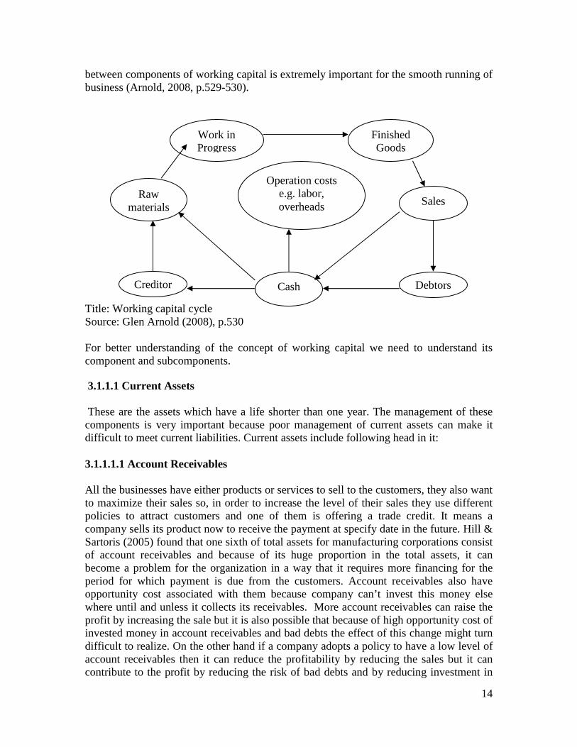
In order to understand the importance of working capital we need to understand the working capital cycle which is described in books of corporate finance. Working capital cycle includes all the major dimensions of business operations. It is quite clear that a bad management of a single account in this cycle might cause a big trouble for the non living entity which might leads to its death so, the management of working capital and balance

14

between components of working capital is extremely important for the smooth running of business (Arnold, 2008, p.529-530). Title: Working capital cycle Source: Glen Arnold (2008), p.530 For better understanding of the concept of working capital we need to understand its component and subcomponents. 3.1.1.1 Current Assets These are the assets which have a life shorter than one year. The management of these components is very important because poor management of current assets can make it difficult to meet current liabilities. Current assets include following head in it: 3.1.1.1.1 Account Receivables All the businesses have either products or services to sell to the customers, they also want to maximize their sales so, in order to increase the level of their sales they use different policies to attract customers and one of them is offering a trade credit. It means a company sells its product now to receive the payment at specify date in the future. Hill & Sartoris (2005) found that one sixth of total assets for manufacturing corporations consist of account receivables and because of its huge proportion in the total assets, it can become a problem for the organization in a way that it requires more financing for the period for which payment is due from the customers. Account receivables also have opportunity cost associated with them because company can’t invest this money else where until and unless it collects its receivables. More account receivables can raise the profit by increasing the sale but it is also possible that because of high opportunity cost of invested money in account receivables and bad debts the effect of this change might turn difficult to realize. On the other hand if a company adopts a policy to have a low level of account receivables then it can reduce the profitability by reducing the sales but it can contribute to the profit by reducing the risk of bad debts and by reducing investment in

Work in Progress

Operation costs e.g. labor, overheads

Creditor

Raw materials

Cash Debtors

Finished Goods

Sales

15

the receivables (Andrew & Gallagher, 1999, p.465). Companies want to have a level of account receivables which maximizes the profitability. The level of account receivables is largely influenced by the credit policy offered by the company to creditors. Strict policy will reduce the collection period and account receivables and if company offers relaxed credit policy it will raise the level of account receivables. Finance managers follow a three step procedure to decide the level of account receivables (Andrew & Gallagher, 1999, p.468).

Step 1: For each proposed credit policy, pro-forma financial statements are developed.

Step 2: For every proposed policy incremental cash flow is estimated by using the pro forma financial statements.

Step 3: NPV is calculated for all the incremental cash flow and the proposed policy with the maximum or the highest NPV is selected.

Step one involves the review of financial statements like balance sheet and income statement and by making necessary changes in these statements, as required by the proposed policy, new financial statements are prepared. In the second step incremental cash flow is calculated by using the new financial statements. Step three involves the comparison of all the proposed policy by calculating the NPV of incremental cash flow by using the following formula (Andrew & Gallagher, 1999, p.470) PVP = PMT *(1/K) Net present value = PVP- Initial investment

Where, PMT is the cash flow of a period and k represents the discount rate or required rate of return. Proposed policy with highest value of NPV will be accepted and adopted as a new credit policy (Andrew & Gallagher, 1999, p.472). 3.1.1.1.2 Inventory Inventory is an important component of current assets. It comprises raw material, finished goods and work in process. It is not necessary for a firm to hold high level of raw material inventory, in fact a firm can order raw material on the daily basis but the high ordering cost is associated with such a policy. Moreover, the delay in supply might stop the production. Similarly, firm can reduce its finished goods inventory by reducing the production and by producing the goods only to meet the current demand but such a strategy can also create trouble for the company if the demand for the product rises suddenly. Such a situation might cause the customer dissatisfaction and even a loyal customer can switch to the competitors brand. Therefore, the firm should have enough inventories to meet the unexpected rise in demand but the cost of holding this inventory should not exceed its benefit (Brealey & Myers, 2006, p.821). Companies want to keep the inventory at a level which maximizes the profit and this level is known as optimal level, but what is an optimal level of inventory for a company? In order to answer this question finance managers analyze the cost associated with inventory i.e. carrying cost and ordering cost. Carrying cost involves insurance, warehouse expenses, utility bills,

16

security expenses etc. in short carrying cost involves all the expenses which a firm have to bear for on hand inventory. Ordering cost is a cost that is associated with one order. It includes telephone expenses, management time, and clerical expenses etc. ordering cost is a fixed cost and its affect can be reduced by ordering a big lot but big lot will increase the carrying cost. On the other hand if a finance manager saves the carrying cost by ordering twice or thrice rather then one big lot then ordering cost will increase. In both cases profitability is directly affected. So, in order to find an optimal level managers have to find a balance between cost and benefit associated with different inventory levels. Economic order quantity provides the balance between carrying cost and ordering cost and helps finance manager to find out the quantity of ordering lot by considering the ordering cost, carrying cost and annual usage (Andrew & Gallagher, 1999, p.472:473).

Source: Gitman, 2002, p. 608 The optimal inventory level or change in the current policy about the inventory is decided by the management in three step procedure as we discussed earlier in the account receivables section i.e. first of all pro-forma financial statements are developed for all the proposed levels or policies then incremental cash flow is calculated by using the pro-forma financial statements and then NPV of the incremental cash flow is calculated. The level which gives the higher net present value is selected as an optimal level of inventory (Andrew & Gallagher, 1999, p.474). 3.1.1.1.3 Short term Investments These are the investments in the money markets and it includes short term securities, T-bills, commercial papers etc. Whenever a firm needs some cash more than its cash reserves it produces cash by liquidating its investments. Investments are treated as primary reserves or secondary reserves for liquidity purposes. Furthermore investment in the money market is considered as a good utilization of idle cash resource which gives return (Hill & Sartoris, 1995), p.288). Finance managers should consider the short term interest rate, transaction cost and market conditions before making any investment. If the benefit of investment is equal to its cost then it doesn’t worth to invest money. 3.1.1.1.4 Cash Cash includes both cash in hand and cash at bank. A company needs cash for transaction and speculation purpose. It also provides the liquidity to the company but the question is why company should have cash reserves when it has an option to utilize it by investing it in short term securities. The answer to this question is that it provides more liquidity then the marketable securities. Cash should be considered as an inventory which is very important for the smooth running of the business. No doubt a company can earn some interest if cash is invested in some marketable securities but when it has to pay its

17

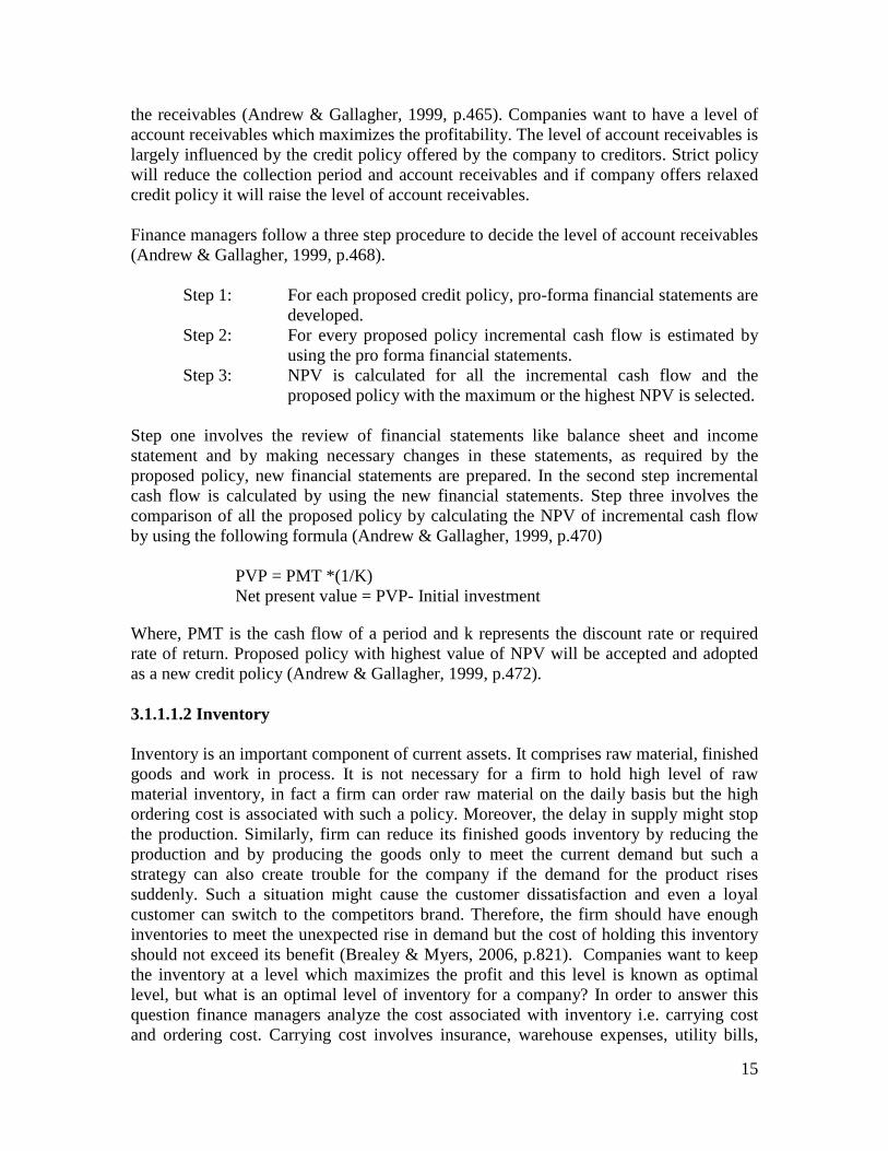
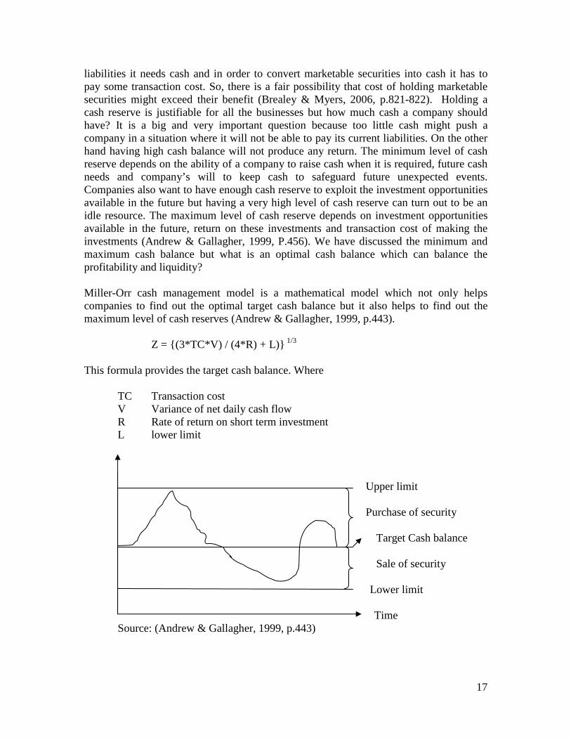
liabilities it needs cash and in order to convert marketable securities into cash it has to pay some transaction cost. So, there is a fair possibility that cost of holding marketable securities might exceed their benefit (Brealey & Myers, 2006, p.821-822). Holding a cash reserve is justifiable for all the businesses but how much cash a company should have? It is a big and very important question because too little cash might push a company in a situation where it will not be able to pay its current liabilities. On the other hand having high cash balance will not produce any return. The minimum level of cash reserve depends on the ability of a company to raise cash when it is required, future cash needs and company’s will to keep cash to safeguard future unexpected events. Companies also want to have enough cash reserve to exploit the investment opportunities available in the future but having a very high level of cash reserve can turn out to be an idle resource. The maximum level of cash reserve depends on investment opportunities available in the future, return on these investments and transaction cost of making the investments (Andrew & Gallagher, 1999, P.456). We have discussed the minimum and maximum cash balance but what is an optimal cash balance which can balance the profitability and liquidity? Miller-Orr cash management model is a mathematical model which not only helps companies to find out the optimal target cash balance but it also helps to find out the maximum level of cash reserves (Andrew & Gallagher, 1999, p.443).

Z = {(3*TC*V) / (4*R) + L)} 1/3

This formula provides the target cash balance. Where

TC Transaction cost V Variance of net daily cash flow R Rate of return on short term investment L lower limit

Upper limit Purchase of security Target Cash balance Sale of security Lower limit Time

Source: (Andrew & Gallagher, 1999, p.443)

18

Miller-Orr also established the formula for upper limit or maximum cash balance (Andrew & Gallagher, 1999, p.444).

Maximum cash balance = 3Z-2L

Management of a company decides on the Minimum balance or lower cash limits by keeping in mind the factors we discussed earlier. According to Miller-Orr if a company has more cash than target cash balance then it will purchase securities to reduce the level of cash and if it have fewer cash resources than the target cash flow then it will sell the securities. The important thing in this model is that a cash balance should fall within the two prescribed limits (Andrew & Gallagher, 1999, p.444). 3.1.1.2 Current Liabilities These are the obligations with a maturity date less than one year. It is very important component of balance sheet which needs to be managed carefully. It includes following: 3.1.1.2.1 Accounts Payables It is the cheapest and simplest way of financing an organization. Account payables are generated when company purchases some products for which payment has to be made no later then a specified date in the future. Account payables are a part of all the businesses and have some advantages associated with it e.g. it is available to all the companies regardless of the size of the company and earlier payment can bring cash discount with it (Arnold, 2008, p.479-482). Companies not only need to manage their account payables in a good way but they should also have the ability to generate enough cash to pay the mature account payables because if a company fails to generate enough cash to fulfill the mature account payables then such a situation will pass the negative signal to the market and it will directly affect the share price, relationship with creditors and suppliers. In this situation it will be difficult for the company to raise more funds by borrowing money or get more supplies from the suppliers. Such a financial distress will lead to the death of the non living entity. 3.1.1.2.2 Short term Borrowings These are the short term financing instruments which a company uses and it includes bank overdraft, commercial papers, bill of exchange, and loan from commercial finance companies etc. All these liabilities have a maturity less than one year (Arnold, 2008, P.474:479). One reason for which company should have a proper working capital policy is short term borrowings because a poor working capital policy might cause the cash distress as a result company might not be able to pay its short term borrowing liability. The consequence of this default can be destructive for a business because after such a situation a company will not be able to win the trust of other financial institutions to borrow more money, market will perceive this situation in a negative way and the value of the share will fall, suppliers and creditors might hesitate to enter in a new contract.

19

3.1.2 Importance of working capital management Working capital has two components current assets and current liabilities. A proper management of working capital is required because if a company has too little investment in the working capital then it means that company doesn’t have sufficient quantity of materials and account receivables which might lead to loss in production and consequently sales will decrease, furthermore in case of a high demand in the market it will be difficult for the company to react immediately and fulfill the demand. On the other hand if the investment in working capital is too big then a company has to bear the cost of storage of inventory, handling cost and opportunity cost (Arnold, 2008, p.529). In order to control risk and cost of the company the decision about the financing and level of working capital is really important. The level of working capital fluctuates with any fluctuation in its component e.g. if the production of firm is higher but the sale is relatively lower than level of inventory will increase, on the other hand if sale exceeds the level of production then inventory will decrease. Similarly, the level of cash will increase when companies collect the receivables and its level reduces when it pays its account payables. Moreover companies have three options to choose between to finance working capital i.e. short term debt, long term debt and equity finance. Equity financing is the most expensive way of financing followed by long term debt and short term debt. Although short term debt is the cheapest way to finance but it carries risk with it because any discarded fluctuation in cash might push the company towards default. Long term debts have more risk then short term debts and it carries high interest rate (because of a higher risk premium) which will reduce profitability. So in order to maintain cash inflow, cash outflow and to create the breakeven between risk, return and liquidity it is really important to manage working capital (Andrew & Gallagher, 1999, p.423:426). 3.1.3 Working Capital Policy Working capital policy can be best described as a strategy which provides the guideline to manage the current assets and current liabilities in such a way that it reduces the risk of default (Brian, 2009). Working capital policy is mainly focusing on the liquidity of current assets to meet current liabilities. Liquidity is very important because if the level of liquidity is too high than a company has lot of idle resources and it has to bear the cost of these idle resources but if the liquidity is too low than it will face lack of resources to meet its current financial liabilities (Vishnani & Shah, 2007). Current assets are key component of working capital and the WCP also depends on the level of current assets against the level of current liabilities (Afza & Nazir, 2007). On this base the literature of finance classifies working capital policy into three categories (Arnold, 2008, p.535-536).

• Aggressive policy • Defensive policy • Conservative policy

A company follows defensive policy by using long term debt and equity to finance its fixed assets and major portion of current assets. Resultantly the level of working capital

20

is quite high which means that a company has more liquid or current assets then the current liabilities. This approach reduces the risk by reducing the current liabilities but it also affects profitability because long term debt offers high interest rate which will increase the cost of financing (Andrew & Gallagher, 1999, p.428). It means a company is not willing to take risk and feel it appropriate to keep cash or near cash balances, higher inventories and generous credit terms. Mostly the companies that are operating in an uncertain environment prefer to adopt such a policy because they are not sure about the future prices, demand and short term interest rate. In such a situation it is better to have a high level of current assets e.g. to keep the higher level of inventory in the stock to meet the sudden rise in demand and to avoid the risk of stoppage in the production. This policy gives a longer cash conversion cycle for the company. Defensive policy provides the shield against the financial distress created by the lack of funds to meet the short term liability but as we discussed earlier long term debt have high interest rate which will increase the cost of financing. Similarly funds tie up in a business because of generous credit policy of the company also have its opportunity cost. Hence this policy might reduce the profitability and the cost of following this policy might exceed the benefits of the policy (Arnold, 2008, p.530). A company can follow aggressive policy by financing its current assets with short term debt because it gives the low interest rate but the risk associated with short term debt is higher then the long term debt. This approach is very risky because the difference between short term or liquid assets and short term liabilities turns very little. Furthermore few finance managers take even more risk by financing long term asset with short term debts and this approach push the working capital on the negative side. Managers try to enhance the profitability by paying lesser interest rate but this approach can be proved very risky if the short term interest rate fluctuates or the cash inflow is not enough to fulfill the current liabilities (Andrew & Gallagher, 1999, p.427). Such a policy is adopted by the company which is operating in a stable economy and is quite certain about future cash flows. A company with aggressive working capital policy offers short credit period to customers, holds minimal inventory and has a small amount of cash in hand. This policy increases the risk of default because a company might face a lack of resources to meet the short term liabilities but it also gives a high return as the high return is associated with high risk (Vishnani & Shah, 2007). Some companies want neither to be aggressive by reducing the level of current assets as compared to current liabilities nor to be defensive by increasing the level of current assets as compared to current liabilities. So, In order to balance the risk and return these firms are following the moderate or conservative approach. This approach is a mixture of defensive WCP and aggressive WCP. In this approach temporary current assets, assets which appear on the balance sheet for short period, will be financed by the short term borrowings and long term debts are used to finance fixed assets and permanent current assets. Thus the follower of this approach finds the moderate level of working capital with moderate risk and return (Andrew & Gallagher, 1999, p.429). Moreover this policy not only reduces the risk of default but it also reduces the opportunity cost of additional investment in the current assets.

21

The level of working capital also depends on the level of sales because sales are the source of revenue for any company. Sales can influence working capital in three possible ways: (Arnold, 2008, p.534:535).

• As sales increase working capital will also increase with the same proportion so, the length of cash conversion cycle remains the same.

• As the sales increase working capital increase in a slower rate. • As the sales increase the level of working capital rises in misappropriate manner

i.e. the working capital might raise in a rate more than the rate of increased in the sale.

A company with stable sale or growing sale can adopt the aggressive policy because it has a confidence on its future cash inflows and is confident to pay its short term liabilities at maturity. On the other hand a company with unstable sale or with fluctuation in the sale can’t think of adopting the aggressive policy because it is not sure about its future cash inflows. In such a situation adoption of aggressive policy is similar to committing a suicide. 3.1.4 Cash Conversion Cycle It is a time span between the payment for raw material and the receipt from the sale of goods. For a manufacturing company we can define it more precisely, it is a time for which raw material is kept for the processing plus the time taken by the production process plus the time for which finished goods are kept and sold and the time taken by the debtors to pay their liability, minus the maturity period of account payable. By this definition it is quite clear that longer cash conversion cycle required more investment in the current assets. Furthermore good cash conversion cycle is helpful for the organization to pay its obligations at a right time which will enhance the goodwill of a company. On the other hand a company with poor cash conversion cycle will not able to meet its current financial obligations and will face financial distress. Cash conversion cycle is also used as a gauge to measure the aggressiveness of working capital policy. It is believed that longer cash conversion cycle corresponds to defensive working capital policy and shorter cash conversion cycle corresponds to aggressive working capital policy (Arnold, 2008, p.530:531). 3.1.4.1 Components of CCC 3.1.4.1.1 Collection period or Days account receivables The time between the sale and the receipt of payment is known as trade credit period or days account receivables. It is believed that longer period of collection of account receivables or longer credit period offered by the company results into higher sales, and more sales bring more profit in the business. So, there could exist a relationship between the number of days account receivables and profitability of the firm. On the other hand large time span between the sale and receipt of account receivables requires higher investment in current assets which is considered as an idle resource and have its own

22

opportunity cost. Furthermore cash generated by the sale is used to pay the operating expenses of the company. So in this situation if the credit period offers by the company to its customers is larger than the credit period offered by its creditors then there will be a financial distress which might lead to bankruptcy (Brealey &Myers, 2006, p.814-815). While deciding on the collection period of account receivables finance managers have to consider the following things (Brealey &Myers, 2006, p.814-815)

• How much money company can invest in account receivables? • What will be the procedure of collection? • Does it have enough money to pay its liabilities? • Cost of investment in account receivables should not exceed its benefit?

After answering to all these questions company decides on the credit policy. The process of decision for the credit policy is the same as we discussed earlier in the account receivables section. After going through that procedure, company will decide the credit policy which will reduce the cost of capital and also provide the suitable collection period. 3.1.4.1.2 Day’s inventory held Day’s inventory held can be defined as the time between the receipt of raw material and delivery of finished goods. It also depends on the policy which a company adopts towards working capital. An aggressive policy of working capital has low inventory level and has few days for which they held inventory. 3.1.4.1.3 Days Account payables Account payables are generated when you buy the product and agree to pay your liability on a specify time in the future. It is a time between the purchase of goods and its payment (Arnold, 2008, p.531). If the firm is unable to pay its account payables on time then it signals to the market that firm have some financial problem and it might go bankrupt resultantly its goodwill will be spoiled and the value of its shares will go down. So, it is necessary for the firm to manage the day’s account payables in a way that it doesn’t create any trouble for it. Shorter duration of day’s account payables can be beneficial for an organization as it has some discount associated with it but at the same time it will force a company to reduce the collection period which might cause the reduction of sale. So, companies have to be very careful while deciding on the duration of day’s account payables. For us it is better for a company to have larger duration of day’s accounts payable than the collection period. 3.1.5 Profitability Profitability is a measure of profit generated from the business and is measured in percentage terms e.g. percentage of sales, percentage of investments, percentage of assets. High percentage of profitability plays a vital role to bring external finance in the

23

business because creditors, investors and suppliers do not hesitate to invest their money in such a company (Gitman, 2002, p.61). 3.1.5.1 Profitability Ratios There are several measures of profitability which a company can use. Few measures of profitability are discussed here. 3.1.5.1.1 Return on Equity (ROE) It measures the earnings of the company against the investment of common stockholders. Shareholders always want the higher value of ROE. It is calculated in the following way (Gitman, 2002, p.65). .

ROE = (Earnings available for common stockholders / CSE)*100 Where, CSE = Common stock equity 3.1.5.1.2 Net Profit Margin It calculates the percentage of each sale dollar remains after deducting interest, dividend, taxes, expenses and costs. In other words it calculates the percentage of profit a company is earning against it’s per dollars sale. Higher value of return on sale shows the better performance (Gitman, 2002, p.64).

NPM = (Earnings available for common stakeholder / N.S)*100

Where, N.S = Net sales

3.1.5.1.3 Return on Total Asset (ROA) This ratio explains that how efficient a company is to utilize its available assets to generate profit. It calculates the percentage of profit a company is earning against per dollar of assets. The higher value of ROA shows the better performance (Gitman, 2002, p.65).

R.O.A = (Earnings available for common stockholders / T.A)*100 Where, T.A = Total Assets 3.1.5.1.4 Gross operation profit This ratio explains that how efficient a company is to utilize its operating assets. This ratio calculates the percentage of profit earned against the operating assets of the company (Lazaridis & tryfonidiens, 2006).

24

Gross operating profit = (Sales – COGS) / (Total asset –financial asset)

3.1.6 Liquidity versus Profitability Creditors of the company always want the company to keep the level of short term assets higher then the level of short term liabilities, this is because they want to secure their money. If current assets are in excess to current liabilities then the creditors will be in a comfortable situation. On the other hand managers of the company don’t think in the same way, obviously each and every manager want to pay the mature liabilities but they also know that excess of current assets might be costly and idle resource which will not produce any return e.g. having high level of inventory will raise warehouse expense So, rather than keeping excessive current assets (cash, inventory, account receivable) they want to keep the optimal level of current assets, a level which is enough to fulfill the current liabilities, and want to invest the excessive amount to earn some return. Now managers have to make a choice between two extreme positions, either they will choose the long term investments, investments in non current asset such as subsidiaries, with high profitability i.e. high return and low liquidity or short term investment with low profitability i.e. low return and high liquidity. Creditors of the company want managers to invest in short term assets because they are easy to liquidate but it reduces the profitability because of low interest rate. On the other hand if the managers prefer the long term investment to enhance the profitability then in case of default lenders or creditors have to wait longer and bear some expense to sell these assets because the liquidity of long term investment is low. In reality, none of the managers choose any of these two extremes instead they want to have a balance between profitability and liquidity which will fulfill their need of liquidity and gives required level of profitability (Andrew & Gallagher, 1999, p.425). 3.1.7 Financial assets Financial assets are intangible assets and can be converted into cash easily. It includes cash, a right under a contract to receive other financial assets or cash from the other enterprise, a right under a contract to exchange financial instruments under favorable conditions with another enterprise, equity of other company and financial instruments (Elliot, 2006, p.172). Financial instruments such as derivatives are part of financial assets under a favorable condition, in an unfavorable condition it might turn into financial liability. Financial assets enhance the profitability as they bring some return in the form of dividend or provide the shield against the risk of certain kind (exchange rate risk, price risk etc). Higher level of financial assets means that companies have higher level of liquidity. If an uncertain event disturbed the cash flow of the company even then company doesn’t need to borrow money on unfavorable terms to pay its liabilities rather it can sell the financial assets.

25

3.1.8 Financial Debt These are the obligation of the company under a contract to deliver cash, financial assets or exchange of financial instrument under an unfavorable condition. All the loan of the company also falls in this category. Financial obligations can be settled with the payment of cash, with the financial assets of the company or share equity of the company (Elliot, 2006, p.172). Financial liabilities also contribute to the profitability as it reduces the cost of issuing share. Timely payment of financial obligations also earns goodwill for the company. 3.2 WC Practice in different geographical areas As we discussed earlier working capital policy can contribute to the profitability of the company. So, each and every company tries to adopt such a policy which gives the competitive edge and enhance profitability. According to Laumus & Williams (1984) the amount which a company invests in working capital can differ from one industrial sector to another. It can also vary between two companies of the same sector. Despite the importance of the issue very little research had been carried out. Almost all the academic literature covers the issue of working capital management, different policies of management and components of working capital but unfortunately none of them explores in-depth its relation with profitability. Literature seems to take for granted that a good working capital policy is needed and creates value. In this section we categorize the previous researches on the topic on the base of the geographical region because people from different geography have different level of risk aversion and different psychology. Moreover political and economic situation in different geographical regions are different. We believe that these factors directly affect the choice of the working capital policy. So, the choice of manager in a stable economy and political situation will differ from that of finance manager who is working in an unstable economy and political situation. Similarly, it is also possible that a same finance manager choose different policies in different geographical region e.g. a finance manager who is following aggressive working capital policy in U.S will not follow the same policy in Iran, Iraq, Afghanistan, India and Pakistan. Thus, the association between working capital policy and profitability in different geographies can also differ. 3.2.1 WC practice in Developing Asian countries Chiou and Cheng (2006) focused on Taiwan to find out the factors which determine the working capital and can affect the management of working capital. They use the quarterly data for the period 1998-2004. They conclude that not only internal factor affect the decision about the working capital management but also there are few outside factors which can directly affect it. These factors are still to be addressed in a proper way. Inside factors have more influence on this decision and they include debt ratio, size of the company, profitability, growth and operating cash flow.

26

Rehman & Nasr (2007) took the sample of 94 companies among the companies which are listed on Karachi stock exchange over the period of 6 years (1999-2004) to study the trend of Pakistani firms towards the working capital and impact of their practice on the profit. They took size of the company, current ratio, debt ratio, net operating profit, cash conversion cycle and component of cash conversion cycle as variables. As a control variable they use financial asset to total asset ratio. Regression analysis and Pearson’s correlation techniques were used for the purpose of analysis. They found that cash makes the major part of the current asset of Pakistani firms. Furthermore they also found the negative relationship between profitability and components of cash conversion cycle. According to them shareholders wealth can be increased by reducing the length of cash conversion cycle. Similar study was conducted by Rahim and Anwer in Malaysia which validate the result of Rehman and Nasr. Vishnani and Shah (2007) investigate the impact on profitability by different working capital policy of 23 listed companies of India in the consumer electronics industry. For their study they focused the period of 10 years (1995-2005). They try to find the relationship between profitability and liquidity i.e. ROCE and current ratio. They find that profitability and liquidity have positive relationship between them but this relationship is very weak because 9 out of 23 companies show negative relationship so, there is no significant relationship exists between liquidity and profitability. They also found the inverse relationship between collection period, holding period and ROCE. Nazir and Talat (2008) study the trend in Pakistani firms towards the working capital policy by using the panel data for 204 non financial firms listed in Karachi stock exchange the period 1998-2005. They found that value can be created by following the conservative approach. Furthermore investors prefer those firms who have aggressive approach towards current liabilities management. In addition to this they explain that manager can increase the shareholder’s wealth by following the aggressive approach but they can’t raise the accounting performance with the same approach In another study Talat and Nazir (2008) studied 208 listed companies on Karachi stock exchange to find out the relationship among the aggressive and conservative policy of working capital. The result contradicts the result of the other studies discussed before. They found that there exist no considerable connection between the aggressiveness of working capital policy and profitability 3.2.2 WC practice in European Companies Deloff (2003) while studying Belgian firms for the period 1992-1996 finds that days A/R, days A/P and stock have negative relationship with profitability. According to him firms can create value by decreasing the amount invested in the current asset to a reasonable level and by shortening their number of days A/R and number of day’s inventory held Lazaridis and Tryfonidis (2006) focused on Athens stock exchange and study 131 listed companies over the period of 2001-2004 to investigate the impact of efficient working capital management on profitability. They used gross operating profit as a measure of

27

profitability. Unlike the previous researches they used CCC, size of the company, fixed financial assets and financial debt ratio as independent variable. The result was similar to the previous studies in a way that firms profitability and cash conversion cycle are negatively correlated. Teruel and Solano (2007) study the trend of working capital of Small and Medium enterprises of Spain. For this purpose they collect the data for 8872 firms for the period 1996-2002. They used ROA as a dependent variable and number of days A/R, number of days A/P and number of day’s inventory held and cash conversion cycle as independent variable. Furthermore size of the firm, growth of sales is used as control variable. They find inverse relationship between number of days A/R and number of day’s inventory held with the profitability of SME. This means that if a company has large inventory and large collection period then it will reduce the profitability. They also found that short CCC will enhance profitability. We had discussed earlier in the report that CCC is used as a measure of degree of aggressiveness of working capital policy. Thus this study indirectly indicates that aggressive WCP can enhance the profitability. Uyar (2009) tried to establish a relationship between CCC, profitability and size of the firm. The focused was on listed companies on Istanbul Stock exchange, he collected the data for 166 companies from seven different industries for the period of one year (2007). He used total asset and net sale as a variable to measure the size and ROE as a variable to measure profitability. ANOVA and Pearson correlation was run to find out the association of CCC with size of the company and CCC with profitability. Not surprisingly there exists a negative relationship between CCC and size of the firm, and CCC and profitability. Samiloglu and Demirgunes (2008) also considered Turkish firms for their study. Not only their study validates the findings of Uyar, they also found that profitability and growth in sales moves in a direct relationship with each other. 3.2.3 WC practice in US In order to discover the relation between cash conversion cycle and profitability Shin and Soenen (1998) focused on listed American firms for the time 1975-1994 to find out the relationship between cash conversion cycle and firms profitability. The result of the study shows that there exists strong negative relationship between the two variables of study, so profitability can be increased by the reduction in cash conversion cycle. Lamberson (1995) tries to find out the impact of change in economic activity on the WCMP. He studied the 50 small firms of US over the period of twelve years (1980-1991). He concludes that the firms are consistent with their investment in working capital and this investment did not increase during the period of economic expansion so, there is a very little impact on WC practice of small firms by the change in economic activities Jose and Lancaster (1996) analyzed 2,718 US firms from different sectors over the period of 18 years (1974-1993) in order to establish a relationship between aggressive WCP and profitability. The result shows the inverse relationship between ROA and WCMP. They

28

also found that the size of the company have nothing to do with such a relationship which contradicts Uyar (2009). Weinraub and Visscher (1998) analyzed the quarterly data of 216 firms from ten different industries to find out practice of different industries towards the working capital. He finds that different industries have different approach towards WCP and there is inverse relationship between liability and asset management. According to him conservative WC financial management always balanced the effect of relative aggressive WC asset management. Ganesan (2007) studied the impact of working capital management policy on the profitability of telecommunication industry of USA. He studied 349 companies over the period of six years (2001-2007). Correlation analysis, regression analysis and ANOVA analysis was conducted to check the impact on profitability by the WCMP, .the result shows the weak negative relation between profitability and WCMP. They find that the companies have poor approach to manage the components of working capital. 3.2.4 Empirical studies in Scandinavia After surfing a lot on the internet and going through different journals we were surprised to know that despite the importance of the topic very little research has been carried out in Scandinavia for an international user i.e. research in English and we were also unable to identify a single research on this subject in Scandinavia. In the second section of this chapter we have discussed all the empirical studies which we found. It provides the guideline for the selection of different variables, as it discussed the variables considered by other researchers to study the same topic. Most of the studies used CCC as a measure of aggressiveness of working capital policy and as an independent variable. Beside this they also used firm size, financial asset ratio and financial debt ration as independent variables. As to the dependent variable, researchers choose between gross operating profit, return on equity and return on asset as a measure of profitability. The results of the studies are different from each other in a way that companies from US, Europe, SMEs and majority of the studies from the developing Asian countries show that profitability and aggressiveness of working capital policy are negatively associated, while the studies from Talat and Nazir (2008) and Vishnani and Shah (2007) shows no association between profitability and aggressiveness of working capital policy. So, it becomes interesting to know how the profitability of the Swedish companies is associated with the working capital policy. This section is an important part of the report in a way that it helps us to develop our research frame work. It not only helps us to identify our variables but also gives us a good idea of our research hypothesis.

29

4. Results & Analysis

This chapter includes Research variables, Hypothesis and Fundamental concepts for analysis. Moreover, in this section we analyze our collected data in SPSS software. Descriptive statistics, Correlation and Regression analysis of collected data is performed in this section. This section gives the answer to our research question. At the end of this chapter you will find the discussion about results. 4.1 Variables 4.1.1 Independent Variable As we have discussed earlier that CCC is a useful measure of degree of aggressiveness of working capital policy i.e. shorter CCC means the company is following aggressive working capital policy and longer cash conversion cycle indicates that a company has adopted defensive working capital policy (Lazaridis & tryfonidiens, 2006). So, in order to find out a relationship between working capital policy and profitability CCC is used as an independent variable for regression analysis. This will be calculated in the following way (Lazaridis & tryfonidiens, 2006):

CCC = Number of days account receivable + Number of days inventory – Number of days account payable

CCC will be used as an independent variable in three different regressions. In first regression we will use sample CCC but in second and third regression CCC of subgroups will be used to explore the association between WCP and profitability. Furthermore we will also try to find the impact of each component of cash conversion cycle on the profitability of the firm. So, each component of working capital will be treated as independent variable and will replace cash conversion cycle in the regression analysis. We calculated the component of cash conversion cycle in the following way (Lazaridis & tryfonidiens, 2006).

No of days Account receivable = (Account receivable * 365) / Sale No of days Inventory = (Inventory * 365) / Cost of goods sold No of days Account payable = (Account payable * 365) /Cost of goods sold

There are many factors which determine the profit of the company. So, in addition to CCC, and components of CCC we will use size of the firm, ratio of fixed financial asset to total asset and financial debt ratio as independent variable in all regressions. Size of the firm is calculated by taking the natural log of sale, financial debt ratio and ratio of fixed financial asset to total asset was calculated in the following way (Lazaridis & tryfonidiens, 2006).

30

Financial debt ratio = financial debt / total asset Financial debt includes both short term and long term loans. Financial debt ratio helps to understand and explain the relationship between total assets and external financing (Lazaridis & tryfonidiens, 2006). Financial asset Ratio = financial asset / total asset This ratio is used as significant part of total assets for the listed companies includes financial assets in it. It includes the investment in the shares of other companies, shares in associated companies, assets held for sale, derivatives and assets available for sale (Lazaridis & tryfonidiens, 2006). For the calculation of financial assets and financial debts we used the following formulas.

Financial assets = investments in equity + financial receivables + asset held for sale + derivatives + marketable securities + other receivables + assets available for sale

Financial debts = long term mortgage + short term mortgage + short term loans + long term loans

4.1.2 Dependent Variable The dependent variable for this research is gross operating profit. We select gross operating profit over return on assets because most of the listed firms have financial assets in their total assets. In such case the return on total asset because of operating activity is minimal. Furthermore we want to correlate operating profit or operating loss with operating assets so, in such case gross operating profit is perfect measure because it excludes all the financing activity from operating activity by subtracting financial assets from total assets. It will be calculated in the following way (Lazaridis & tryfonidiens, 2006). Gross operating profit = (Sales – COGS) / (Total assets – financial assets) We used Microsoft excel to do all the calculations, for our dependent and independent variables, before the analysis in the SPSS (Appendix 1). 4.2 Hypothesis We have discussed earlier that we will use GOP (Dependent Variable) as a measure of profitability and CCC (Independent variable) as a measure of degree of aggressiveness of working capital policy. Therefore, in our hypothesis we will also use these variables to define the relationship between profitability and working capital policy. Furthermore we will also develop a hypothesis to find out the relationship of profitability with days

31

account receivables, days account payables and days inventory held. Thus, we will have six hypotheses which will be tested by a regression analysis later on. 4.2.1 Hypothesis 1 As we want to find out the relationship between profitability and working capital policy and we are using CCC as a measure of aggressiveness of working capital policy and GOP as a measure of profitability so, the first hypothesis will test the relationship between CCC and GOP of our sample.

H1 there exist a relationship between GOPs and CCCs.

The alternative to this hypothesis is

H0 There exist no relationship between GOPs and CCCs. We will analyze the data by a regression analysis in a SPSS and the value of un-standardized coefficient which is represented by ß will explain the nature of the relationship. Following is the regression model for first hypothesis.

H1 ßcccs ≠ 0 H0 ßcccs = 0

If ß will be greater than or less than zero then there exist positive or negative relationship between profitability (GOPs) and working capital policy (CCCs). If ß is equal to zero than there exist no relationship between the variables. In such case we will reject our hypothesis. 4.2.2 Hypothesis 2 This hypothesis will explore the relationship between profitability and defensive working capital policy. So the association between GOPD and CCCD of defensive group will be explained in this regression.

H1 There exist a relationship between GOPD and CCCD of defensive group.

The alternative to this hypothesis is

H0 There exist no relationship between GOPD and CCCD of defensive group. If ß will be greater than or less than zero then null hypothesis will be neglected and the positive or negative sign with the value of ßcccd will explain the nature of the relationship. Following is the model for hypothesis.

H1 ßcccd ≠ 0 H0 ßcccd = 0

32

4.2.3 Hypothesis 3 The association between the profitability and working capital policy of aggressive group will be test in this regression. So, the relationship between GOP and CCC of aggressive group will be explained in this hypothesis.

H1 Tthere exist a relationship between GOPA and CCCA of aggressive group.

The alternative to this hypothesis is

H0 There exist no relationship between GOPA and CCCA of aggressive group. The value of ß will explain the nature of the relationship.

H1 ßccca ≠ 0 H0 ßccca = 0

4.2.4 Hypothesis 4 Fourth hypothesis will check the relationship between profitability and days account receivables.

H1 There exist a relationship between GOP (Profitability) and days Account receivables of an organization.

The alternative to the hypothesis is

H0 There exist no relationship between GOP (profitability) and days account receivables.

We will do regression again and the value of ß will explain the nature of relationship. Regression model for this hypothesis is as under.

H1 ßAR ≠ 0 H0 ßAR = 0

4.2.5 Hypothesis 5 Fifth hypothesis will be tested, in order to find out the association between profitability and days account payables.

H1 There is some association between GOP (profitability) and days account payables.

Alternative approach to this hypothesis is

33

H0 There is no association between GOP (profitability) and days account payables. The value of the ß will be obtained by regression analysis which will explain the nature of the relationship. Following is the regression model for this hypothesis.

H1 ßAP ≠ 0 H0 ßAP = 0

4.2.6 Hypothesis 6 This hypothesis will test the relationship between profitability and day’s inventory held.

H1 There is some affiliation between GOP (profitability) and day’s inventory held.

Null hypothesis for this relationship states:

H0 There is no affiliation between GOP (profitability) and days inventory held. The regression analysis will provide the value of ß which will explain the relationship between these two variables.

H1 ßINV ≠ 0 H0 ßINV = 0

4.3 Fundamental Concepts for Analysis 4.3.1 F value The value of F test explains the overall significance of a model. It explains the significance of the relationship between dependent variables and all the other independent variables. (Anderson et al., 2007, p.573) 4.3.2 T Value T value is used to determine the level of significance of regression coefficient. It is also known as test of individual significance. It explains the significance of relationship between dependent variable with each of the independent variable. If the t value is less than 3 than it supports the null hypothesis and if the t value is greater than 3 then it neglects the null hypothesis (Anderson et al., 2007, p.574). 4.3.3 R square It explains the total variation in the value of dependent variable. Its value lies between 0 and 1, if the value of R square is closer to 1 than it tells that the regression model which is applied on data really supports it (Kohler, 1994, p.600).

34

4.3.4 P Value It is also used to determine the level of significance of regression coefficient. It measures whether the data supports the null hypothesis or not. If the P value is greater than .05 then null hypotheses can’t be rejected and if the value of P is less than .05 than it rejects the null hypothesis. Usually we call it significance. (Anderson et al., 2007, p.573) 4.3.5 95 % Confidence Interval It gives two boundaries where a certain percentage of population is expected to lay e.g. 95% confidence interval means that 95 % of the population will lay between the upper boundary and lower boundary and half of the remaining values lie above the upper boundary and half of it lies below the lower boundary (Kohler, 1994, p.636). 4.3.6 Durbin Watson Test This test is used in a regression analysis to find out the autocorrelation in the residuals. The values of Durbin Watson have a upper limit of four and lower limit of zero. If the value of Durban Watson is equal to two then there exists no autocorrelation but if the value is less than two then there exists positive correlation and if the value is higher than 2 than there exist negative correlation (Kohler, 1994, p.634). 4.3.7 Correlation Correlation explains how two variables react to each other e.g. what change will occur in one variable with the change in other variable (Kohler, 1994, p.550). 4.3.8 Beta (ß) The value of beta explain the change in the dependent variable with the per unit change in independent variable. It also explains the nature and strength of the relationship between dependent variable and independent variable (Malhotra, 2004, p.513). A hypothesis will be accepted or rejected on the base of ß value because value of ß explains the relationship between dependent variable and independent variable. However, the significance of a relationship between dependent variable and individual independent variable will be tested by the T value and P value. F value and significance level (P value) will test the authenticity of regression model for the data. Total variation in dependent variable because of regression model will be explained by the R square. Durbin Watson will test the autocorrelation between the independent variables.

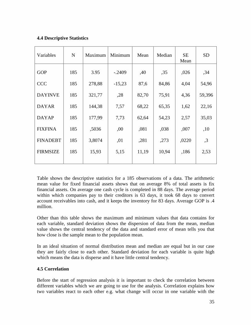
35

4.4 Descriptive Statistics Variables

N

Maximum

Minimum

Mean

Median

SE

Mean

SD

GOP CCC DAYINVE DAYAR DAYAP FIXFINA FINADEBT FIRMSIZE

185

185

185

185

185

185

185

185

3.95

278,88

321,77

144,38

177,99

,5036

3,8074

15,93

-.2409

-15,23

,28

7,57

7,73

,00

,01

5,15

,40

87,6

82,70

68,22

62,64

,081

,281

11,19

,35

84,86

75,91

65,35

54,23

,038

,273

10,94

,026

4,04

4,36

1,62

2,57

,007

,0220

,186

,34

54,96

59,396

22,16

35,03

,10

,3

2,53

Table shows the descriptive statistics for a 185 observations of a data. The arithmetic mean value for fixed financial assets shows that on average 8% of total assets is fix financial assets. On average one cash cycle is completed in 88 days. The average period within which companies pay to their creditors is 63 days, it took 68 days to convert account receivables into cash, and it keeps the inventory for 83 days. Average GOP is .4 million. Other than this table shows the maximum and minimum values that data contains for each variable, standard deviation shows the dispersion of data from the mean, median value shows the central tendency of the data and standard error of mean tells you that how close is the sample mean to the population mean. In an ideal situation of normal distribution mean and median are equal but in our case they are fairly close to each other. Standard deviation for each variable is quite high which means the data is disperse and it have little central tendency. 4.5 Correlation Before the start of regression analysis it is important to check the correlation between different variables which we are going to use for the analysis. Correlation explains how two variables react to each other e.g. what change will occur in one variable with the

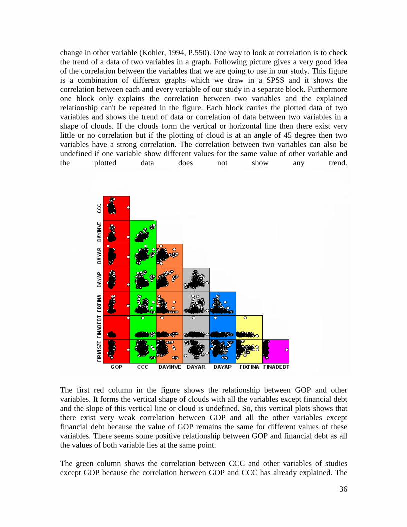
36

change in other variable (Kohler, 1994, P.550). One way to look at correlation is to check the trend of a data of two variables in a graph. Following picture gives a very good idea of the correlation between the variables that we are going to use in our study. This figure is a combination of different graphs which we draw in a SPSS and it shows the correlation between each and every variable of our study in a separate block. Furthermore one block only explains the correlation between two variables and the explained relationship can't be repeated in the figure. Each block carries the plotted data of two variables and shows the trend of data or correlation of data between two variables in a shape of clouds. If the clouds form the vertical or horizontal line then there exist very little or no correlation but if the plotting of cloud is at an angle of 45 degree then two variables have a strong correlation. The correlation between two variables can also be undefined if one variable show different values for the same value of other variable and the plotted data does not show any trend.

The first red column in the figure shows the relationship between GOP and other variables. It forms the vertical shape of clouds with all the variables except financial debt and the slope of this vertical line or cloud is undefined. So, this vertical plots shows that there exist very weak correlation between GOP and all the other variables except financial debt because the value of GOP remains the same for different values of these variables. There seems some positive relationship between GOP and financial debt as all the values of both variable lies at the same point. The green column shows the correlation between CCC and other variables of studies except GOP because the correlation between GOP and CCC has already explained. The

37

correlation of cash conversion cycle with the component of cash conversion cycle (days account receivable, inventory and days accounts payable), fixed financial assets and firm size is undefined because of the strange plotting of data i.e. for one value of CCC these variables shows different values. However correlation between CCC and financial debt is very weak because any variation in the value of cash conversion cycle doesn’t bring a big change in the value of financial debt. Brown column shows the correlation of day’s inventory held with other variables of the study. Figure shows that there exist some correlation between days inventory held with days account payable and day’s account receivables but this relationship is undefined i.e. days account payable and days account receivables show different values for one value of days inventory held . Plotted data in other blocks of brown column shows that days inventory held don’t have any correlation with firm size and fixed financial asset. Correlation between days inventory held and financial debt is very weak because financial debt almost have the same value for different values of day’s inventory held. Correlation of days account receivable is shown in the grey column. This column shows that there exist some correlation between days account receivable and days account payables but this correlation is undefined and difficult to read. Similarly correlation of account receivables with fixed financial assets and firm size is undefined. Moreover, financial debt has a very week correlation with day’s account receivables. Days account payables have undefined correlation with firm size as shown by blue column. This column also shows that there exists no correlation between days account payable and fixed financial assets. Yellow column shows the correlation of fixed financial assets with financial debt and firm size. The figure shows that financial debt has very week correlation with fixed financial asset and it has undefined correlation with the firm size. Pink column shows the weak correlation between financial debt and size of the firm. In the figure above one thing is common in all the columns and that is the correlation of financial debt with other variables. Financial debts have a very week correlation with other variables and the slope of the plotted data of its correlation with other variables in different columns is indefinite. For the better understanding of correlation between different variables we used Pearson correlation. It shows that there exist very little positive relationship between GOP and CCC and it is consistent with the view that a relax credit terms or larger credit period offer by the company will result into more sale and more sale will bring more profit. GOP is also positively correlated with the day’s inventory held and day’s account payables but it is negatively correlated with day’s account receivables and firm size but these correlations are also very weak. CCC is positively correlated with all the other variables except firm size. Its relationship with all other variables is very weak except with days inventory held because it has strong positive correlation (.832) with it. Furthermore all the other variables are also

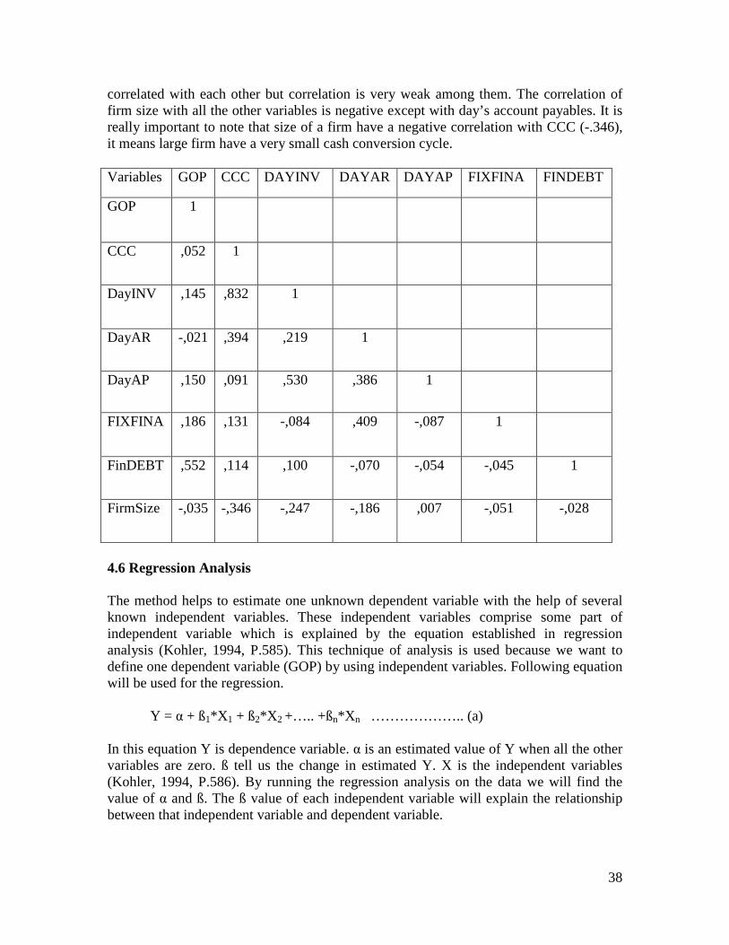
38

correlated with each other but correlation is very weak among them. The correlation of firm size with all the other variables is negative except with day’s account payables. It is really important to note that size of a firm have a negative correlation with CCC (-.346), it means large firm have a very small cash conversion cycle. Variables GOP CCC DAYINV DAYAR DAYAP FIXFINA FINDEBT

GOP

1

CCC

,052

1

DayINV

,145

,832

1

DayAR

-,021

,394

,219

1

DayAP

,150

,091

,530

,386

1

FIXFINA

,186

,131

-,084

,409

-,087

1

FinDEBT

,552

,114

,100

-,070

-,054

-,045

1

FirmSize

-,035

-,346

-,247

-,186

,007

-,051

-,028

4.6 Regression Analysis The method helps to estimate one unknown dependent variable with the help of several known independent variables. These independent variables comprise some part of independent variable which is explained by the equation established in regression analysis (Kohler, 1994, P.585). This technique of analysis is used because we want to define one dependent variable (GOP) by using independent variables. Following equation will be used for the regression. Y = α + ß1*X 1 + ß2*X 2 +….. +ßn*X n ……………….. (a) In this equation Y is dependence variable. α is an estimated value of Y when all the other variables are zero. ß tell us the change in estimated Y. X is the independent variables (Kohler, 1994, P.586). By running the regression analysis on the data we will find the value of α and ß. The ß value of each independent variable will explain the relationship between that independent variable and dependent variable.

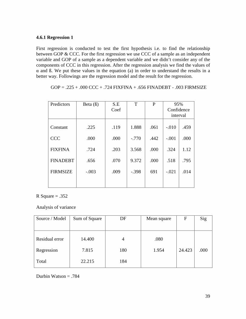
39

4.6.1 Regression 1 First regression is conducted to test the first hypothesis i.e. to find the relationship between GOP & CCC. For the first regression we use CCC of a sample as an independent variable and GOP of a sample as a dependent variable and we didn’t consider any of the components of CCC in this regression. After the regression analysis we find the values of α and ß. We put these values in the equation (a) in order to understand the results in a better way. Followings are the regression model and the result for the regression. GOP = .225 + .000 CCC + .724 FIXFINA + .656 FINADEBT - .003 FIRMSIZE

Predictors Beta (ß) S.E Coef

T P 95% Confidence

interval Constant CCC FIXFINA FINADEBT FIRMSIZE

.225

.000

.724

.656

-.003

.119

.000

.203

.070

.009

1.888

-.770

3.568

9.372

-.398

.061

.442

.000

.000

691

-.010

-.001

.324

.518

-.021

.459

.000

1.12

.795

.014

R Square = .352 Analysis of variance Source / Model Sum of Square DF Mean square F Sig

Residual error Regression Total

14.400

7.815

22.215

4

180

184

.080

1.954

24.423

.000

Durbin Watson = .784

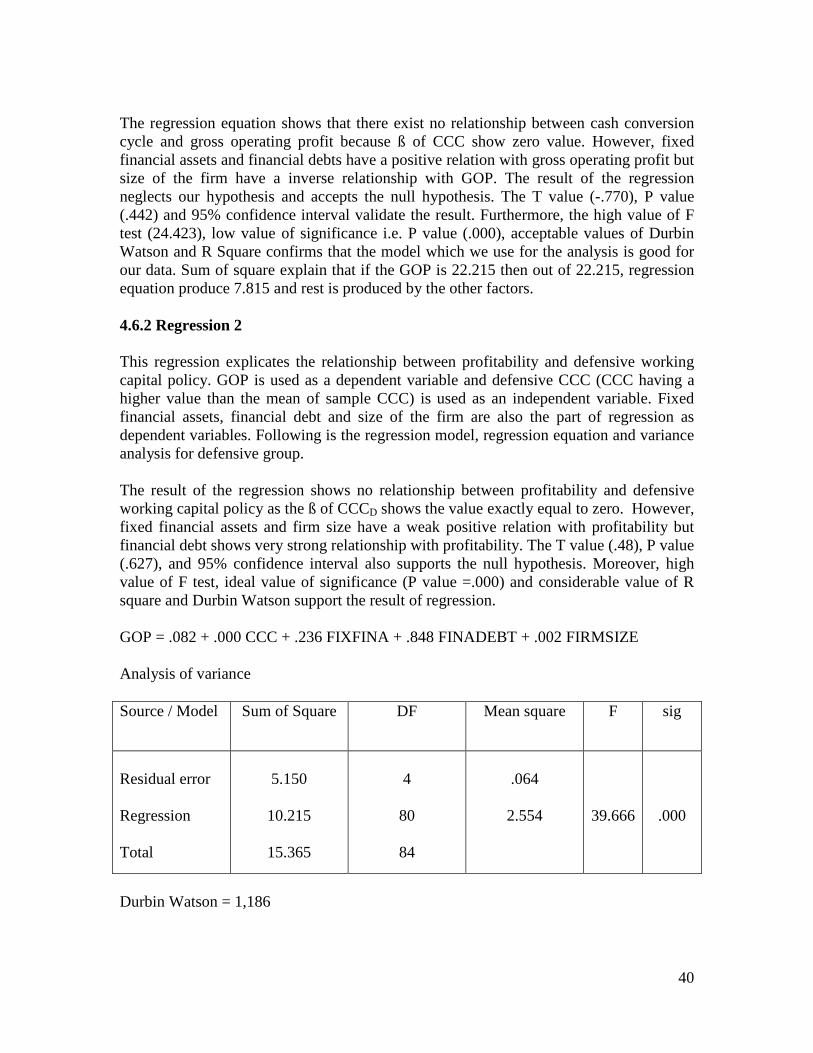
40

The regression equation shows that there exist no relationship between cash conversion cycle and gross operating profit because ß of CCC show zero value. However, fixed financial assets and financial debts have a positive relation with gross operating profit but size of the firm have a inverse relationship with GOP. The result of the regression neglects our hypothesis and accepts the null hypothesis. The T value (-.770), P value (.442) and 95% confidence interval validate the result. Furthermore, the high value of F test (24.423), low value of significance i.e. P value (.000), acceptable values of Durbin Watson and R Square confirms that the model which we use for the analysis is good for our data. Sum of square explain that if the GOP is 22.215 then out of 22.215, regression equation produce 7.815 and rest is produced by the other factors. 4.6.2 Regression 2 This regression explicates the relationship between profitability and defensive working capital policy. GOP is used as a dependent variable and defensive CCC (CCC having a higher value than the mean of sample CCC) is used as an independent variable. Fixed financial assets, financial debt and size of the firm are also the part of regression as dependent variables. Following is the regression model, regression equation and variance analysis for defensive group. The result of the regression shows no relationship between profitability and defensive working capital policy as the ß of CCCD shows the value exactly equal to zero. However, fixed financial assets and firm size have a weak positive relation with profitability but financial debt shows very strong relationship with profitability. The T value (.48), P value (.627), and 95% confidence interval also supports the null hypothesis. Moreover, high value of F test, ideal value of significance (P value =.000) and considerable value of R square and Durbin Watson support the result of regression. GOP = .082 + .000 CCC + .236 FIXFINA + .848 FINADEBT + .002 FIRMSIZE Analysis of variance Source / Model Sum of Square DF Mean square F sig

Residual error Regression Total

5.150

10.215

15.365

4

80

84

.064

2.554

39.666

.000

Durbin Watson = 1,186

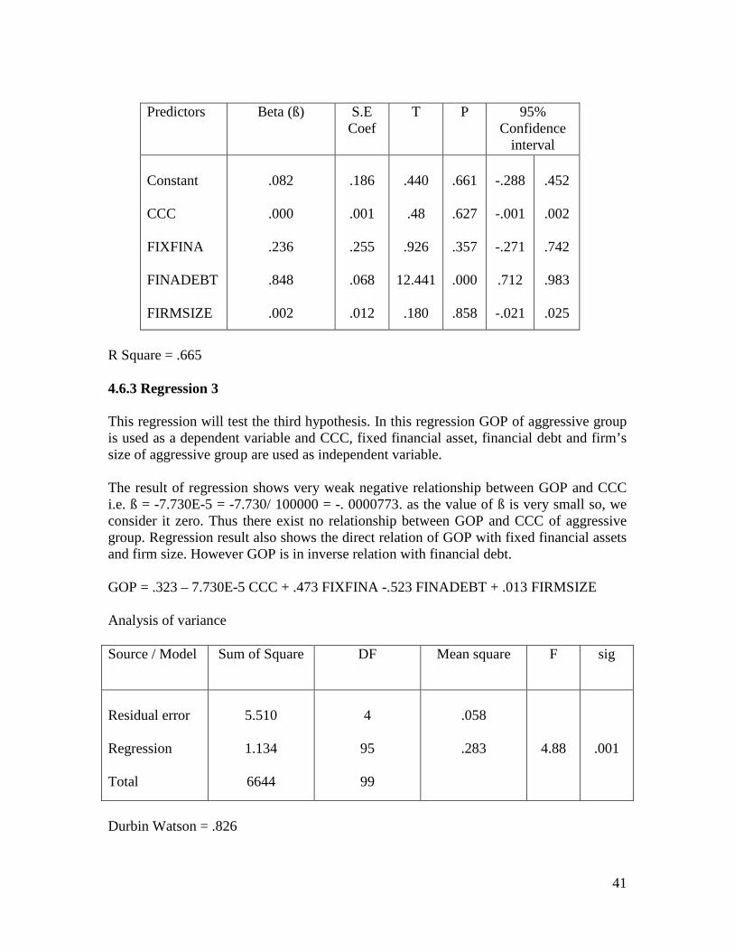
41

Predictors Beta (ß) S.E

Coef T P 95%

Confidence interval

Constant CCC FIXFINA FINADEBT FIRMSIZE

.082

.000

.236

.848

.002

.186

.001

.255

.068

.012

.440

.48

.926

12.441

.180

.661

.627

.357

.000

.858

-.288

-.001

-.271

.712

-.021

.452

.002

.742

.983

.025

R Square = .665 4.6.3 Regression 3 This regression will test the third hypothesis. In this regression GOP of aggressive group is used as a dependent variable and CCC, fixed financial asset, financial debt and firm’s size of aggressive group are used as independent variable. The result of regression shows very weak negative relationship between GOP and CCC i.e. ß = -7.730E-5 = -7.730/ 100000 = -. 0000773. as the value of ß is very small so, we consider it zero. Thus there exist no relationship between GOP and CCC of aggressive group. Regression result also shows the direct relation of GOP with fixed financial assets and firm size. However GOP is in inverse relation with financial debt. GOP = .323 – 7.730E-5 CCC + .473 FIXFINA -.523 FINADEBT + .013 FIRMSIZE Analysis of variance Source / Model Sum of Square DF Mean square F sig

Residual error Regression Total

5.510

1.134

6644

4

95

99

.058

.283

4.88

.001

Durbin Watson = .826

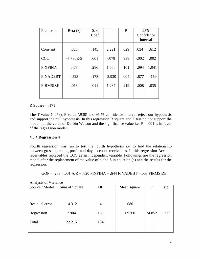
42

Predictors Beta (ß) S.E

Coef T P 95%

Confidence interval

Constant CCC FIXFINA FINADEBT FIRMSIZE

.323

-7.730E-5

.473

-.523

.013

.145

.001

.286

.178

.011

2.221

-.078

1.658

-2.930

1.237

.029

.938

.101

.004

.219

.034

-.002

-.094

-.877

-.008

.612

.002

1.041

-.169

.035

R Square = .171 The T value (-.078), P value (.938) and 95 % confidence interval reject our hypothesis and support the null hypothesis. In this regression R square and F test do not support the model but the value of Durbin Watson and the significance value i.e. P = .001 is in favor of the regression model. 4.6.4 Regression 4 Fourth regression was run to test the fourth hypothesis i.e. to find the relationship between gross operating profit and days account receivables. In this regression Account receivables replaced the CCC as an independent variable. Followings are the regression model after the replacement of the value of α and ß in equation (a) and the results for the regression.

GOP = .283 - .001 A/R + .820 FIXFINA + .644 FINADEBT - .003 FIRMSIZE Analysis of Variance Source / Model Sum of Square DF Mean square F sig

Residual error Regression Total

14.312

7.904

22.215

4

180

184

.080

1.9760

24.852

.000

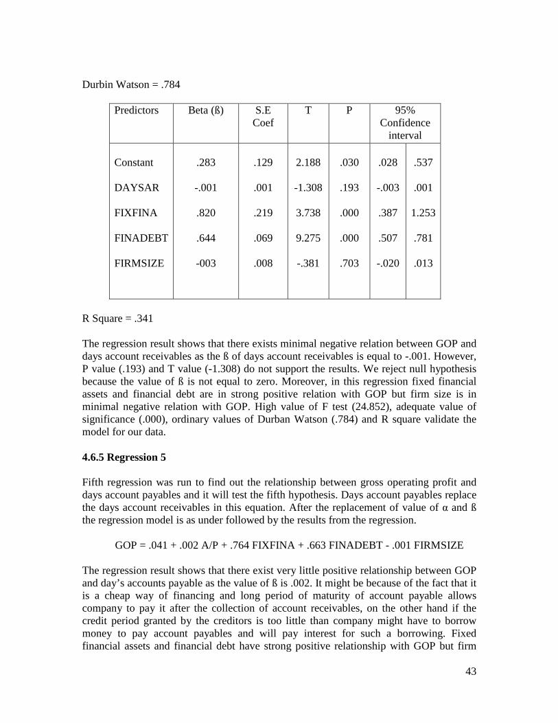
43

Durbin Watson = .784

Predictors Beta (ß) S.E Coef

T P 95% Confidence

interval Constant DAYSAR FIXFINA FINADEBT FIRMSIZE

.283

-.001

.820

.644

-003

.129

.001

.219

.069

.008

2.188

-1.308

3.738

9.275

-.381

.030

.193

.000

.000

.703

.028

-.003

.387

.507

-.020

.537

.001

1.253

.781

.013

R Square = .341 The regression result shows that there exists minimal negative relation between GOP and days account receivables as the ß of days account receivables is equal to -.001. However, P value (.193) and T value (-1.308) do not support the results. We reject null hypothesis because the value of ß is not equal to zero. Moreover, in this regression fixed financial assets and financial debt are in strong positive relation with GOP but firm size is in minimal negative relation with GOP. High value of F test (24.852), adequate value of significance (.000), ordinary values of Durban Watson (.784) and R square validate the model for our data. 4.6.5 Regression 5 Fifth regression was run to find out the relationship between gross operating profit and days account payables and it will test the fifth hypothesis. Days account payables replace the days account receivables in this equation. After the replacement of value of α and ß the regression model is as under followed by the results from the regression.

GOP = .041 + .002 A/P + .764 FIXFINA + .663 FINADEBT - .001 FIRMSIZE The regression result shows that there exist very little positive relationship between GOP and day’s accounts payable as the value of ß is .002. It might be because of the fact that it is a cheap way of financing and long period of maturity of account payable allows company to pay it after the collection of account receivables, on the other hand if the credit period granted by the creditors is too little than company might have to borrow money to pay account payables and will pay interest for such a borrowing. Fixed financial assets and financial debt have strong positive relationship with GOP but firm

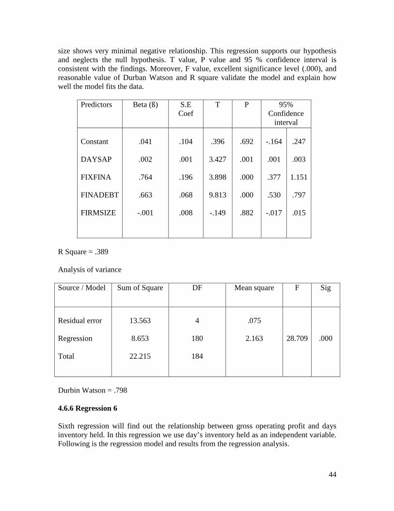
44

size shows very minimal negative relationship. This regression supports our hypothesis and neglects the null hypothesis. T value, P value and 95 % confidence interval is consistent with the findings. Moreover, F value, excellent significance level (.000), and reasonable value of Durban Watson and R square validate the model and explain how well the model fits the data.

Predictors Beta (ß) S.E Coef

T P 95% Confidence

interval Constant DAYSAP FIXFINA FINADEBT FIRMSIZE

.041

.002

.764

.663

-.001

.104

.001

.196

.068

.008

.396

3.427

3.898

9.813

-.149

.692

.001

.000

.000

.882

-.164

.001

.377

.530

-.017

.247

.003

1.151

.797

.015

R Square = .389 Analysis of variance Source / Model Sum of Square DF Mean square F Sig

Residual error Regression Total

13.563

8.653

22.215

4

180

184

.075

2.163

28.709

.000

Durbin Watson = .798 4.6.6 Regression 6 Sixth regression will find out the relationship between gross operating profit and days inventory held. In this regression we use day’s inventory held as an independent variable. Following is the regression model and results from the regression analysis.

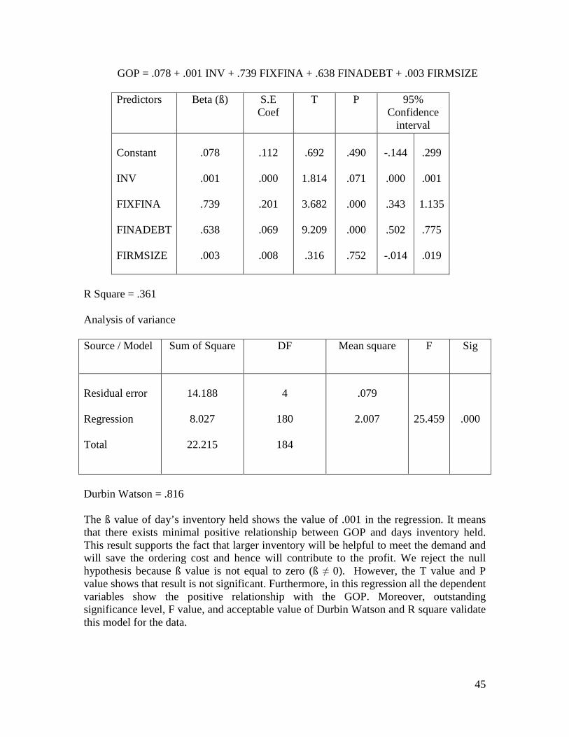
45

GOP = .078 + .001 INV + .739 FIXFINA + .638 FINADEBT + .003 FIRMSIZE

Predictors Beta (ß) S.E Coef

T P 95% Confidence

interval Constant INV FIXFINA FINADEBT FIRMSIZE

.078

.001

.739

.638

.003

.112

.000

.201

.069

.008

.692

1.814

3.682

9.209

.316

.490

.071

.000

.000

.752

-.144

.000

.343

.502

-.014

.299

.001

1.135

.775

.019

R Square = .361 Analysis of variance Source / Model Sum of Square DF Mean square F Sig

Residual error Regression Total

14.188

8.027

22.215

4

180

184

.079

2.007

25.459

.000

Durbin Watson = .816 The ß value of day’s inventory held shows the value of .001 in the regression. It means that there exists minimal positive relationship between GOP and days inventory held. This result supports the fact that larger inventory will be helpful to meet the demand and will save the ordering cost and hence will contribute to the profit. We reject the null hypothesis because ß value is not equal to zero (ß ≠ 0). However, the T value and P value shows that result is not significant. Furthermore, in this regression all the dependent variables show the positive relationship with the GOP. Moreover, outstanding significance level, F value, and acceptable value of Durbin Watson and R square validate this model for the data.

46

4.7 Discussion In this study we tried three different ways to establish a relationship between working capital policy and profitability. First of all we took the working capital policy of our sample and tried to find its association with the profitability. Then we divide our sample into subgroups (Aggressive group and Defensive group) and tried to establish a relationship between the profitability of the subgroup with the relative working capital policy. After three regressions we found that there is no association between the profitability and working capital policy because the ß value which explains the relationship between CCC and GOP shows the value of zero in all three regressions. There are two possibilities for which ß can show the value exactly equal to zero, either the data contains the statistical error which can be corrected by revising the data or the values in the data are correct but in reality there exist no relationship between the two variables. The result of this regression forced us to revise our data to check whether data contains the statistical error or the regression analysis shows the true relationship. Revision of data authenticates the results of regression. The outcome of the regression analysis shows that there exist no relationship between working capital policy and profitability of Swedish companies because regression analysis was unable to find out any association between the variables we used to measure profitability and degree of aggressiveness of working capital policy. The result is consistent with the findings of Vishnani & Shah (2007) and Nazir & Talat (2008) Since CCC didn’t have any association with GOP, it became really interested to know that whether its component has some association with the GOP or not. In order to fine out the association between component of cash conversion cycle and profitability of the company three more regressions was run. In regression four Days account receivables replaced the CCC as an independent variable. As a result of regression analysis we found that there is minimal negative correlation between the day’s account receivables and GOP. The result is consistent with the view that small collection period save the opportunity cost and helps company to pay its liabilities by its own money rather than borrowing money at some interest. Outcome of regression five and six shows that GOP is directly associated with days inventory held and day’s account payables but these associations are very week. The result of fifth regression is consistent with the view that longer payment period of account payables contribute to the profit by reducing borrowing cost because it is a cheap way of financing and long period of maturity of account payable allows company to pay it after the collection of account receivables. The result of sixth regression supports the view that higher inventory contributes to the profit by reducing ordering cost and by providing a shield against the stoppage of production in case of high demand. We also found that fixed financial asset and financial debt have a direct relation with gross operating profit but size of the firm have an inverse relationship with GOP. We had discussed earlier that short term financial debt are the cheapest way to finance a business and can raise the profitability this fact is supported by regression results.

47

5. Credibility Criteria

This chapter will check the level of credibility of this research. There are three ways to check the credibility and we will go through all three of them and will see whether our research fulfills the requirements of these three measures of credibility or not. 5.1 Reliability Reliability means that the result will be the same even if another researcher will carry out the research on a different occasion. Furthermore the research should not be subject bias, observer bias and it should not have any subject error (Saunders & Lewis, 2000, P.100:101). As we gather all data from the audited financial reports of the companies and the analysis was conducted in SPSS software. This analysis and data are neither subject biased nor observer biased. It is also not possible to change the values of different accounts in financial statements. Thus if the research will be repeated by someone else then it will give the same result. 5.2 Validity Validity means the findings of a research are real e.g. the research conducted to explain the relationship between two variables will show the same relationship as it is in reality and there exist no fictitious numbers to make the result attractive (Saunders & Lewis, 2000, P.101:102) . The data which we used for the analysis was from the financial reports provided by the companies in their annual reports, the data belongs to real world, and there are no factious figures to make the result more interesting. It is explaining the true and real relationship between profitability and working capital policy of the Swedish companies. 5.3 Generalization It is also known as external validity. It explains that to which extent the results of your research are applicable to other research settings. If the research is not conducted with the intention to find or develop a theory which can be generalized then one could explain that what is actually happening in your research settings (Saunders & Lewis, 2000, P102:103). As we discussed earlier the data is not fictitious and SPSS software was used to explain the relationship between two variables, thus we believe that the results of the study are applicable to other research settings.

48

6. Further research

This research tried to meet the gap between the existing literatures but it also has its limitations and those limitations can be addressed by the researchers in the future. This research is different from other researches in a way that it is a first effort to find out the relationship between the profitability and working capital policy in any of the Scandinavian countries as it focused Sweden to find out this relationship. More research work can be carried out in other Scandinavian countries to find out this relationship. It would be really interesting to know whether this relationship change within the Scandinavian countries or not. While working on this report we faced the language constraint and because of lack of knowledge of Swedish language we were unable to extract data from the balance sheet of those companies which have their financial reports in Swedish. So, such companies with financial reports in Swedish are not part of this study. We suggest the Swedish students to work on the same topic by including all the non financial companies, even the companies which have their financial reports in Swedish, in their sample. Moreover, this research only uses one measure to measure the profitability and degree of aggressiveness of working capital policy. However there are lots of measures of profitability (ROA, ROI etc) and degree of aggressiveness of the working capital policy (Current Ratio).More research can be carried out by considering different measures of profitability and degree of aggressiveness of working capital policy in order to explore the relationship between working capital policy and profitability of the firm. Results can differ from this study by the use of different measures of profitability and degree of aggressiveness of working capital policy. We have discussed earlier that working capital policy of the company depends on many factors e.g. sales, economic situations, political situations and profitability. More research can be conducted to find the affect of these factors on the working capital policy. In order to find out the relationship between working capital policy and profitability most of the empirical studies focused on the accounting measures of profitability. Research can be repeated by considering the performance measures of profitability e.g. economic value added, market value added etc.

49

7. Conclusion

This study has examined the relationship between working capital policy and profitability of Swedish firms. We took a sample of 37 companies which are listed at OMX Stockholm stock exchange. In order to correlate the operating profit or operating loss with operating assets we choose GOP as a measure of profitability and CCC is used as a measure of aggressiveness of working capital policy. Moreover we also tried to find the relationship of profitability with the components of CCC. Regression analysis in SPSS software was run to test the six hypotheses. We observed in the first three regressions that there exist no relationship between Sample CCC, aggressive CCC and defensive CCC with their respective GOP. Thus, there is no association between working capital policy and any of the working capital policy. So, managers can’t raise the accounting profit by following any of the working capital policy. However, it might be possible to raise the holding period return with it because a policy towards a working capital passes a signal to market and the market will develop a perception accordingly. Furthermore, we find negative relationship between GOP and days account receivables which make a sense in a way that larger credit period offered by the company to raise the level of the sale in order to earn more profit might result in a higher level of bad debts. Moreover company needs money for smooth running of business operations and high investment in account receivables will force a company to borrow money from financial institutions which will directly affect the profitability. This negative relationship also suggests that less profitable firm are trying to decrease the level of their account receivables in order to meet a cash gap. We also observed that longer account payables period gives higher profit. It is quite logical because we know that account payables are the cheapest way to finance a business and larger duration of account payables will allow a company to offer a larger credit period to its customers that will raise the sale and profitability. In addition it is quite likely that company doesn’t need to borrow money, which will save interest money, to pay its account payables if the maturity period of account payables is larger than the credit period offer by the company to its customers. GOP and days inventory held also have positive relationship which make a sense in a way that higher inventory is needed to meet the higher demand, buying in bulk also reduce the ordering cost and high trade discount is associated with it. Low inventory level might reduce your carrying cost but it will create a trouble in case of sudden rise in demand and if a company will not be able to satisfy the demand of its customer then the customers can switch to the competitors brand and it will decrease the level of sale and profitability. It is quite clear after the analysis of available data that managers can raise the profitability of Swedish companies by using the financial debt to finance its operations, by keeping

50

the level of financial assets at a higher level, by reducing the collection period, by holding more inventory and by prolonging the payment period but they can’t raise the level of profitability by adopting any of the working capital policy. However, a good management of working capital is necessary for the smooth running of business but it has nothing to do with the profitability. The results are not only surprising but it also contradicts the previous studies but after revising data several times and conducting analysis carefully we conclude that Swedish companies are not adjusting the level of working capital in accordance with the sales. Either they didn’t change the level of working capital with the change in sale or if they change it then this change is not associated with sale e.g. the rate of change in working capital is greater than the rate with which sales moves. For us this is the reason that we didn’t find any relationship between WCP and profitability of Swedish companies.

51

8. References

1) Anderson et al., (2007), Statistics for Business and Economics, Thomson Learning.

2) Brealey & Myers (2006), Corporate Finance, Eighth edition, McGraw hill 3) Brian B, (2009) Working capital policy and liquidity in the small business, journal

of small business management, jul7,vol 17, issue3, PP 43-51, Blackwell publisher 4) Brigham & Houston (2007), Fundamentals of Financial Management, 11th Edition

Thomson Coporation. 5) Chiou and Cheng (2006) The determinants of working capital Management , the

journal of American Academy of business 10(1): PP149-155 6) Deloof M (2003). Does Working Capital Management Affect Profitability of

Belgian Firms? Journal of Business, Finance and Accounting 30(3&4): PP 573-587

7) Elliot & Barry, (2006), Financial Accounting Reporting and Analysis, 2nd Edition, Prentice Hall.

8) Filbeck G and T Krueger (2005). Industry Related Differences in Working Capital Management. - 51 -Mid-American Journal of Business 20(2): PP 11-18

9) Gallagher. T & Joseph. A (2000), Financial Management: Principles and Practices with Finance Center Disk, 2nd Edition, Prentice Hall.

10) Ganesan (2007), An Analysis of Working Capital Management Efficiency in Telecommunication equipment industry, River Academic journal 3(2)

11) Gitman, (2002), Principle Of Managerial Finance, 10th Edition, Addison-Wesley 12) Glen, Arnold (2008), corporate financial management, 4the edition, Pearson

education limited 13) Hill & Sartories (1995), Short-term financial management, Third edition, prentice

hall. 14) Jose and Lancaster (1996), Corporate Returns and Cash Conversion

Cycles,Journal of Economics and Finance 20(1):33-46 15) Kohler (1994), statistics for business and economics, third edition, HarperCollins

college publishers 16) Lamberson M (1995). Changes in Working Capital of Small Firms in Relation to

Changes in Economic Activity. Mid-American Journal of Business 10(2): 45-50 17) Laumas and Williams (1984), The demand for working capital, Applied

Economics (16):791-798 18) Lazaridis and tryfonidiens (2006) relationship between working capital

management and profitability of listed companies in the Athens stock exchanges. Journal of Financial Management and Analysis, 26-35

19) Morawski, (2008), Investment Decisions on Illiquid Assets: A Search Theoretical Approach to Real Estate Liquidity, Gabler Edition, Gabler GWV Fachverlage GmbH Wiesbaden.

20) Nazir and Afza (2008), Is it better to be agressvie or Conservative in Manageing Working Capitl, Journal of Quality and Technology Management, Vol 3, No 2, pp.11-21

52

21) Nazri and Afaz (January 02-03, 2008) A panel data analysis of working capital management policies, IBA Business Review, Vol 4, No1, pp143-157

22) Padachi (2006) Trend in working capital management and its impact on firms performance: An Analysis of Mauritian Small Manufacturing Firms, International review of business Research papers 2(2):45-58

23) Rehman and Nasr (2007), Working capital management and profitability-Case of Pakistani firms, International Review of Business Research Papers 3(1):279-300

24) Rahim and Anwar ( 2006), Effect of working capital management on profitability of firms in Malaysia,University Putra Malaysia.

25) Samiloglu and Demirgunes (2008), The effect of working capital management on firm profitability evidence from Turkey, The international Journal of Applied Economics and finance 2(1):44-50

26) Saunders & Lewis (2000), Research Methods for Business Student, Second Edition, Prentice Hall

27) Smith K (1980). Profitability versus Liquidity Tradeoffs in Working Capital Management, in Readings on the Management of Working Capital. New York: St. Paul, West Publishing Company.

28) Shin HH and L Soenen (1998). Efficiency of Working Capital and Corporate Profitability. Financial Practice and Education 8: 37-45.

29) Teruel and Solano (2007) Effects of working capital management on SME profitability, international journal of managerial finance 3(2):164-177

30) Uyar (2009), The relationship of cash conversion cycle with firm size and profitability an empirical investigation in Turkey, International Research journal of finance and economics 24

31) Vishnani S and Shah B (2007), Impact of Working Capital Management Policies on Corporate Performance an empirical study, Global Business Review 2007; 8; 267

32) Weinraub and Visscher (1998), Industry practice relating to aggressive conservative working capital policies, Journal of financial and strategic decisions 11(2)

33) Morawski, (2008), Investment Decisions on Illiquid Assets: A Search Theoretical Approach to Real Estate Liquidity, Gabler Edition, Gabler GWV Fachverlage GmbH Wiesbaden.

Websites

1) www.translate.google.com 2) www.ub.umu.se 3) http://www.nasdaqomxnordic.com/

53

9. Glossary AR Account receivables AP Account payables CCC Cash conversion cycle CCCS Sample cash conversion cycle CCCA Cash conversion cycle of aggressive group CCCD Cash conversion cycle of defensive group DAYSAR Days account receivables DAYSAP Days account payables DAYSINV Days inventory held FIXFINA Fixed financial asset FINADEBT Financial debt FIRMSIZE Firm size GOP Gross operating profit INV Inventory K Discount rate NPV Net present value PVP Present value of perpetuity ROA Return on Assets ROCE Return on common equity SMEs Small and medium enterprises WC Working capital WCP Working capital policy WCMP Working capital management policy

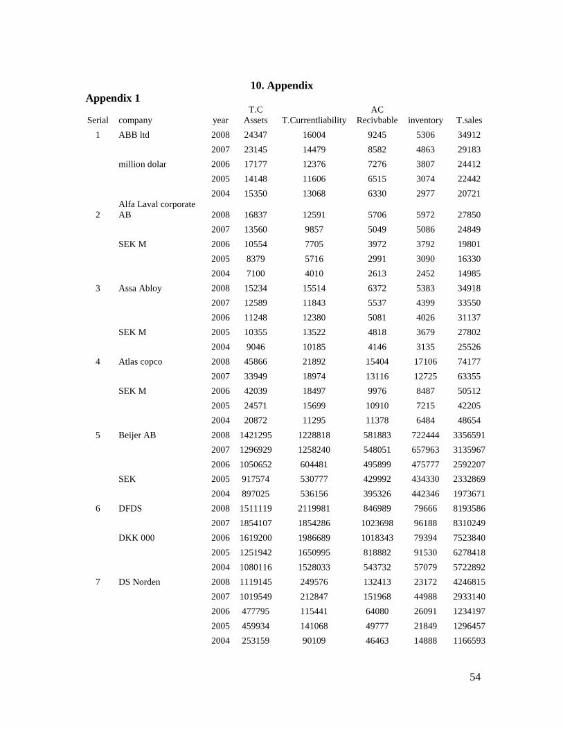
54

10. Appendix

Appendix 1

Serial company year T.C

Assets T.Currentliability AC

Recivbable inventory T.sales

1 ABB ltd 2008 24347 16004 9245 5306 34912

2007 23145 14479 8582 4863 29183

million dolar 2006 17177 12376 7276 3807 24412

2005 14148 11606 6515 3074 22442

2004 15350 13068 6330 2977 20721

2 Alfa Laval corporate AB 2008 16837 12591 5706 5972 27850

2007 13560 9857 5049 5086 24849

SEK M 2006 10554 7705 3972 3792 19801

2005 8379 5716 2991 3090 16330

2004 7100 4010 2613 2452 14985

3 Assa Abloy 2008 15234 15514 6372 5383 34918

2007 12589 11843 5537 4399 33550

2006 11248 12380 5081 4026 31137

SEK M 2005 10355 13522 4818 3679 27802

2004 9046 10185 4146 3135 25526

4 Atlas copco 2008 45866 21892 15404 17106 74177

2007 33949 18974 13116 12725 63355

SEK M 2006 42039 18497 9976 8487 50512

2005 24571 15699 10910 7215 42205

2004 20872 11295 11378 6484 48654

5 Beijer AB 2008 1421295 1228818 581883 722444 3356591

2007 1296929 1258240 548051 657963 3135967

2006 1050652 604481 495899 475777 2592207

SEK 2005 917574 530777 429992 434330 2332869

2004 897025 536156 395326 442346 1973671

6 DFDS 2008 1511119 2119981 846989 79666 8193586

2007 1854107 1854286 1023698 96188 8310249

DKK 000 2006 1619200 1986689 1018343 79394 7523840

2005 1251942 1650995 818882 91530 6278418

2004 1080116 1528033 543732 57079 5722892

7 DS Norden 2008 1119145 249576 132413 23172 4246815

2007 1019549 212847 151968 44988 2933140

2006 477795 115441 64080 26091 1234197

2005 459934 141068 49777 21849 1296457

2004 253159 90109 46463 14888 1166593

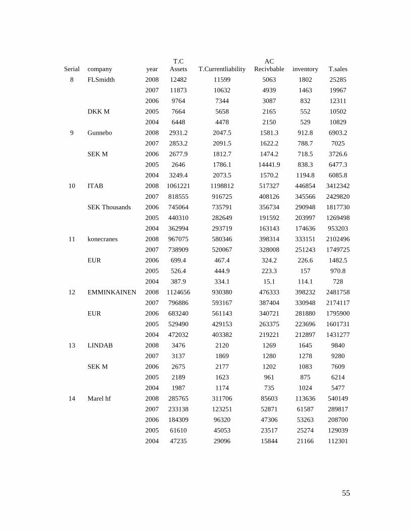
55

Serial company year T.C

Assets T.Currentliability AC

Recivbable inventory T.sales

8 FLSmidth 2008 12482 11599 5063 1802 25285

2007 11873 10632 4939 1463 19967

2006 9764 7344 3087 832 12311

DKK M 2005 7664 5658 2165 552 10502

2004 6448 4478 2150 529 10829

9 Gunnebo 2008 2931.2 2047.5 1581.3 912.8 6903.2

2007 2853.2 2091.5 1622.2 788.7 7025

SEK M 2006 2677.9 1812.7 1474.2 718.5 3726.6

2005 2646 1786.1 14441.9 838.3 6477.3

2004 3249.4 2073.5 1570.2 1194.8 6085.8

10 ITAB 2008 1061221 1198812 517327 446854 3412342

2007 818555 916725 408126 345566 2429820

SEK Thousands 2006 745064 735791 356734 290948 1817730

2005 440310 282649 191592 203997 1269498

2004 362994 293719 163143 174636 953203

11 konecranes 2008 967075 580346 398314 333151 2102496

2007 738909 520067 328008 251243 1749725

EUR 2006 699.4 467.4 324.2 226.6 1482.5

2005 526.4 444.9 223.3 157 970.8

2004 387.9 334.1 15.1 114.1 728

12 EMMINKAINEN 2008 1124656 930380 476333 398232 2481758

2007 796886 593167 387404 330948 2174117

EUR 2006 683240 561143 340721 281880 1795900

2005 529490 429153 263375 223696 1601731

2004 472032 403382 219221 212897 1431277

13 LINDAB 2008 3476 2120 1269 1645 9840

2007 3137 1869 1280 1278 9280

SEK M 2006 2675 2177 1202 1083 7609

2005 2189 1623 961 875 6214

2004 1987 1174 735 1024 5477

14 Marel hf 2008 285765 311706 85603 113636 540149

2007 233138 123251 52871 61587 289817

2006 184309 96320 47306 53263 208700

2005 61610 45053 23517 25274 129039

2004 47235 29096 15844 21166 112301

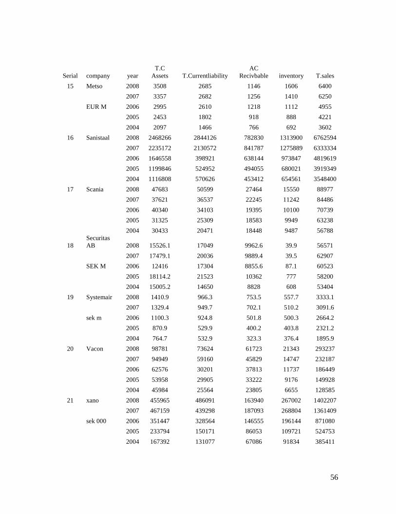
56

Serial company year T.C

Assets T.Currentliability AC

Recivbable inventory T.sales

15 Metso 2008 3508 2685 1146 1606 6400

2007 3357 2682 1256 1410 6250

EUR M 2006 2995 2610 1218 1112 4955

2005 2453 1802 918 888 4221

2004 2097 1466 766 692 3602

16 Sanistaal 2008 2468266 2844126 782830 1313900 6762594

2007 2235172 2130572 841787 1275889 6333334

2006 1646558 398921 638144 973847 4819619

2005 1199846 524952 494055 680021 3919349

2004 1116808 570626 453412 654561 3548400

17 Scania 2008 47683 50599 27464 15550 88977

2007 37621 36537 22245 11242 84486

2006 40340 34103 19395 10100 70739

2005 31325 25309 18583 9949 63238

2004 30433 20471 18448 9487 56788

18 Securitas AB 2008 15526.1 17049 9962.6 39.9 56571

2007 17479.1 20036 9889.4 39.5 62907

SEK M 2006 12416 17304 8855.6 87.1 60523

2005 18114.2 21523 10362 777 58200

2004 15005.2 14650 8828 608 53404

19 Systemair 2008 1410.9 966.3 753.5 557.7 3333.1

2007 1329.4 949.7 702.1 510.2 3091.6

sek m 2006 1100.3 924.8 501.8 500.3 2664.2

2005 870.9 529.9 400.2 403.8 2321.2

2004 764.7 532.9 323.3 376.4 1895.9

20 Vacon 2008 98781 73624 61723 21343 293237

2007 94949 59160 45829 14747 232187

2006 62576 30201 37813 11737 186449

2005 53958 29905 33222 9176 149928

2004 45984 25564 23805 6655 128585

21 xano 2008 455965 486091 163940 267002 1402207

2007 467159 439298 187093 268804 1361409

sek 000 2006 351447 328564 146555 196144 871080

2005 233794 150171 86053 109721 524753

2004 167392 131077 67086 91834 385411

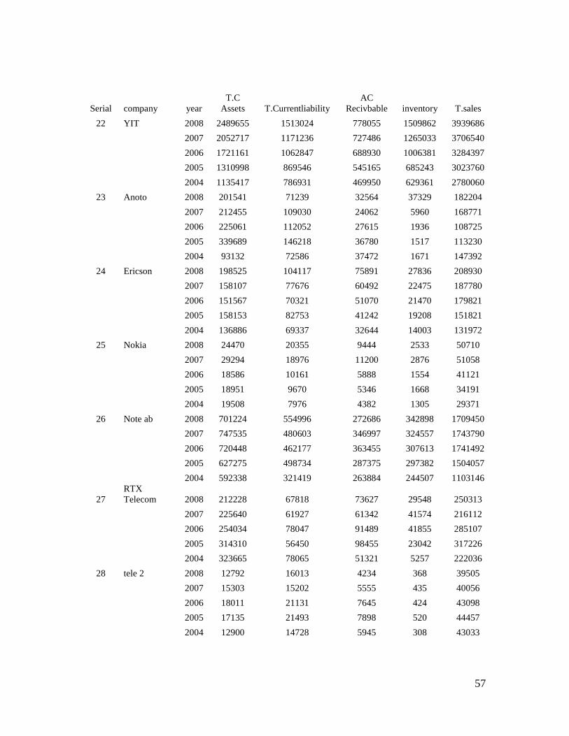
57

Serial company year T.C

Assets T.Currentliability AC

Recivbable inventory T.sales

22 YIT 2008 2489655 1513024 778055 1509862 3939686

2007 2052717 1171236 727486 1265033 3706540

2006 1721161 1062847 688930 1006381 3284397

2005 1310998 869546 545165 685243 3023760

2004 1135417 786931 469950 629361 2780060

23 Anoto 2008 201541 71239 32564 37329 182204

2007 212455 109030 24062 5960 168771

2006 225061 112052 27615 1936 108725

2005 339689 146218 36780 1517 113230

2004 93132 72586 37472 1671 147392

24 Ericson 2008 198525 104117 75891 27836 208930

2007 158107 77676 60492 22475 187780

2006 151567 70321 51070 21470 179821

2005 158153 82753 41242 19208 151821

2004 136886 69337 32644 14003 131972

25 Nokia 2008 24470 20355 9444 2533 50710

2007 29294 18976 11200 2876 51058

2006 18586 10161 5888 1554 41121

2005 18951 9670 5346 1668 34191

2004 19508 7976 4382 1305 29371

26 Note ab 2008 701224 554996 272686 342898 1709450

2007 747535 480603 346997 324557 1743790

2006 720448 462177 363455 307613 1741492

2005 627275 498734 287375 297382 1504057

2004 592338 321419 263884 244507 1103146

27 RTX Telecom 2008 212228 67818 73627 29548 250313

2007 225640 61927 61342 41574 216112

2006 254034 78047 91489 41855 285107

2005 314310 56450 98455 23042 317226

2004 323665 78065 51321 5257 222036

28 tele 2 2008 12792 16013 4234 368 39505

2007 15303 15202 5555 435 40056

2006 18011 21131 7645 424 43098

2005 17135 21493 7898 520 44457

2004 12900 14728 5945 308 43033

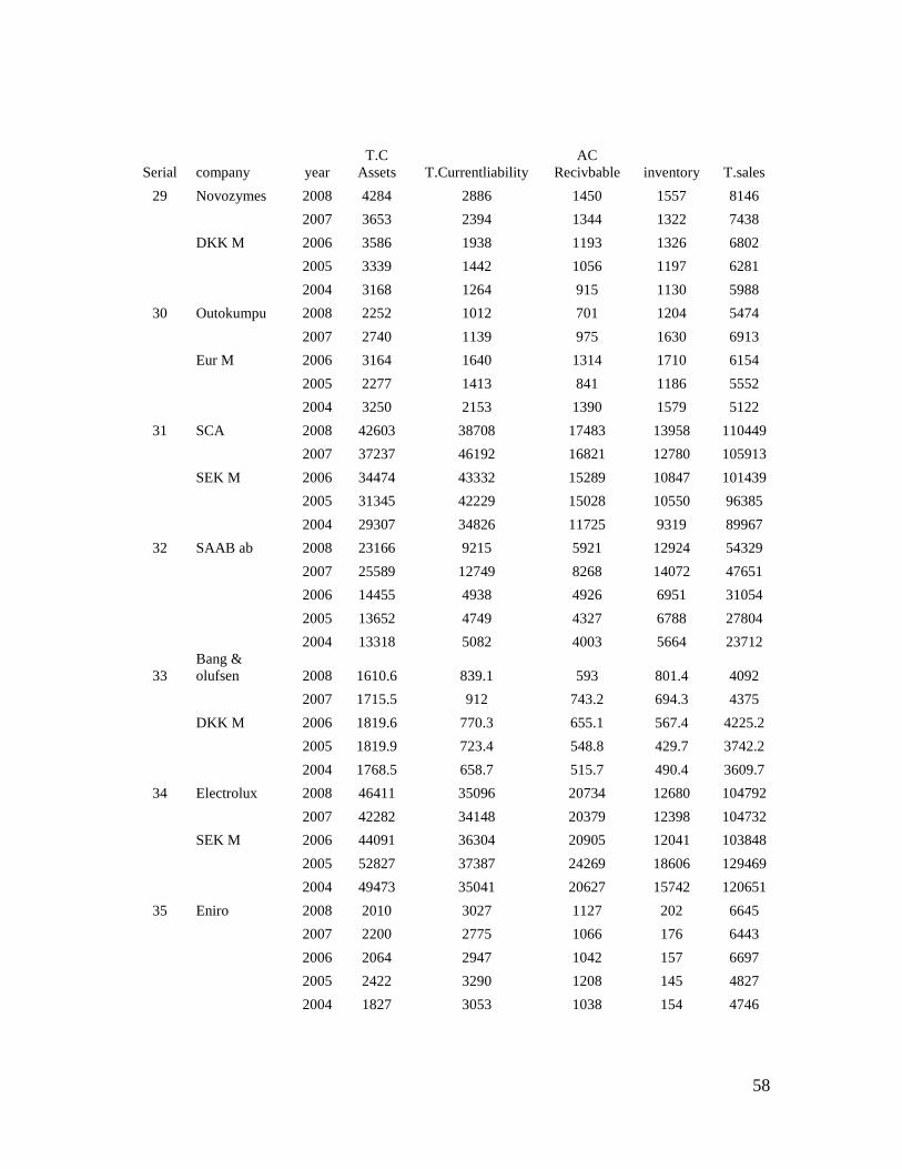
58

Serial company year T.C

Assets T.Currentliability AC

Recivbable inventory T.sales

29 Novozymes 2008 4284 2886 1450 1557 8146

2007 3653 2394 1344 1322 7438

DKK M 2006 3586 1938 1193 1326 6802

2005 3339 1442 1056 1197 6281

2004 3168 1264 915 1130 5988

30 Outokumpu 2008 2252 1012 701 1204 5474

2007 2740 1139 975 1630 6913

Eur M 2006 3164 1640 1314 1710 6154

2005 2277 1413 841 1186 5552

2004 3250 2153 1390 1579 5122

31 SCA 2008 42603 38708 17483 13958 110449

2007 37237 46192 16821 12780 105913

SEK M 2006 34474 43332 15289 10847 101439

2005 31345 42229 15028 10550 96385

2004 29307 34826 11725 9319 89967

32 SAAB ab 2008 23166 9215 5921 12924 54329

2007 25589 12749 8268 14072 47651

2006 14455 4938 4926 6951 31054

2005 13652 4749 4327 6788 27804

2004 13318 5082 4003 5664 23712

33 Bang & olufsen 2008 1610.6 839.1 593 801.4 4092

2007 1715.5 912 743.2 694.3 4375

DKK M 2006 1819.6 770.3 655.1 567.4 4225.2

2005 1819.9 723.4 548.8 429.7 3742.2

2004 1768.5 658.7 515.7 490.4 3609.7

34 Electrolux 2008 46411 35096 20734 12680 104792

2007 42282 34148 20379 12398 104732

SEK M 2006 44091 36304 20905 12041 103848

2005 52827 37387 24269 18606 129469

2004 49473 35041 20627 15742 120651

35 Eniro 2008 2010 3027 1127 202 6645

2007 2200 2775 1066 176 6443

2006 2064 2947 1042 157 6697

2005 2422 3290 1208 145 4827

2004 1827 3053 1038 154 4746

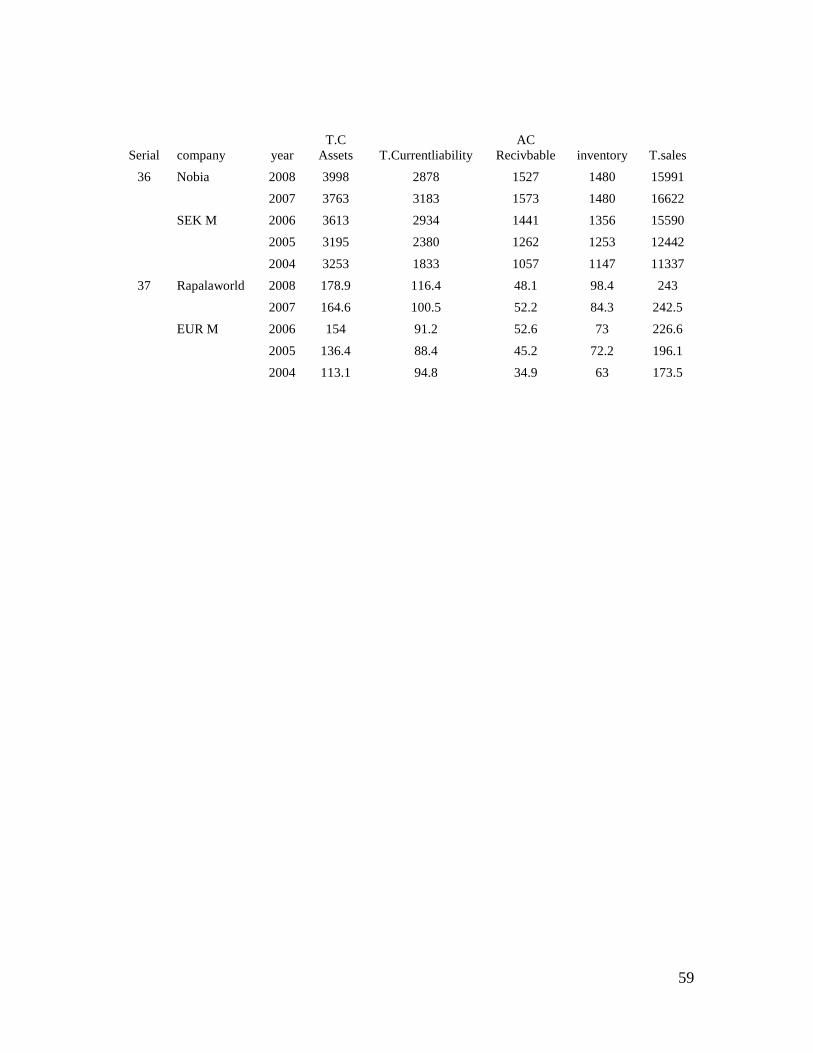
59

Serial company year T.C

Assets T.Currentliability AC

Recivbable inventory T.sales

36 Nobia 2008 3998 2878 1527 1480 15991

2007 3763 3183 1573 1480 16622

SEK M 2006 3613 2934 1441 1356 15590

2005 3195 2380 1262 1253 12442

2004 3253 1833 1057 1147 11337

37 Rapalaworld 2008 178.9 116.4 48.1 98.4 243

2007 164.6 100.5 52.2 84.3 242.5

EUR M 2006 154 91.2 52.6 73 226.6

2005 136.4 88.4 45.2 72.2 196.1

2004 113.1 94.8 34.9 63 173.5

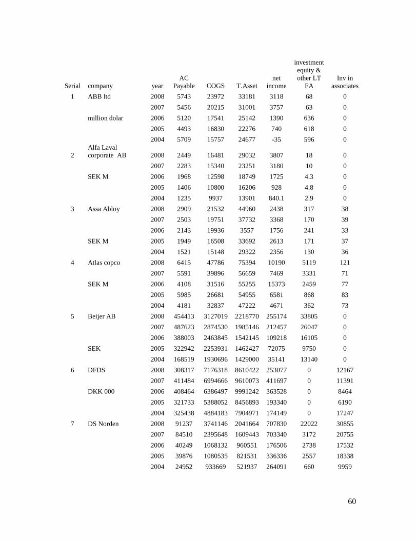
60

Serial company year AC

Payable COGS T.Asset net

income

investment equity & other LT

FA Inv in

associates

1 ABB ltd 2008 5743 23972 33181 3118 68 0

2007 5456 20215 31001 3757 63 0

million dolar 2006 5120 17541 25142 1390 636 0

2005 4493 16830 22276 740 618 0

2004 5709 15757 24677 -35 596 0

2 Alfa Laval corporate AB 2008 2449 16481 29032 3807 18 0

2007 2283 15340 23251 3180 10 0

SEK M 2006 1968 12598 18749 1725 4.3 0

2005 1406 10800 16206 928 4.8 0

2004 1235 9937 13901 840.1 2.9 0

3 Assa Abloy 2008 2909 21532 44960 2438 317 38

2007 2503 19751 37732 3368 170 39

2006 2143 19936 3557 1756 241 33

SEK M 2005 1949 16508 33692 2613 171 37

2004 1521 15148 29322 2356 130 36

4 Atlas copco 2008 6415 47786 75394 10190 5119 121

2007 5591 39896 56659 7469 3331 71

SEK M 2006 4108 31516 55255 15373 2459 77

2005 5985 26681 54955 6581 868 83

2004 4181 32837 47222 4671 362 73

5 Beijer AB 2008 454413 3127019 2218770 255174 33805 0

2007 487623 2874530 1985146 212457 26047 0

2006 388003 2463845 1542145 109218 16105 0

SEK 2005 322942 2253931 1462427 72075 9750 0

2004 168519 1930696 1429000 35141 13140 0

6 DFDS 2008 308317 7176318 8610422 253077 0 12167

2007 411484 6994666 9610073 411697 0 11391

DKK 000 2006 408464 6386497 9991242 363528 0 8464

2005 321733 5388052 8456893 193340 0 6190

2004 325438 4884183 7904971 174149 0 17247

7 DS Norden 2008 91237 3741146 2041664 707830 22022 30855

2007 84510 2395648 1609443 703340 3172 20755

2006 40249 1068132 960551 176506 2738 17532

2005 39876 1080535 821531 336336 2557 18338

2004 24952 933669 521937 264091 660 9959

61

Serial company year AC

Payable COGS T.Asset net

income

investment equity & other LT

FA Inv in

associates

15 Metso 2008 1189 4733 5511 390 0 14

2007 1291 4702 5254 384 0 19

EUR M 2006 1238 3659 4958 410 0 19

2005 925 3110 3904 237 0 20

2004 873 2673 3570 144 1 17

16 Sanistaal 2008 688767 5160005 3902679 -551513 0 227241

2007 567593 4746473 4107258 38178 0 451220

2006 476231 3663857 2188457 158575 0 0

2005 360374 3002804 1655029 118721 0 0

2004 306425 2631416 1549654 139989 0 0

17 Scania 2008 6783 64516 110035 8890 0 495

2007 7068 61810 91454 8554 0 264

2006 6011 52255 88078 5939 0 173

2005 4901 47835 78218 4665 0 96

2004 4167 12528 70703 4316 0 92

18 Securitas AB 2008 977 46122 35718.9 2321 0 104.9

2007 1247 51135 39185.2 526 0 103.5

SEK M 2006 1153 49029 35719.8 852 0 172.7

2005 1560 46781 46280 2713 0 178.6

2004 1411 42758 38850 2529.1 0 0

19 Systemair 2008 479.5 2089.1 2401.4 237.6 0 0

2007 467 1927.4 2168.6 254.6 0 0.1

sek m 2006 207.5 1651.6 1895 170.5 0 0.1

2005 174.2 1459.4 1507.2 97.7 0 0

2004 139.8 1214.8 1329.4 75.9 0 0.1

20 Vacon 2008 37614 150779 149118 23909 0 0

2007 30887 123048 123166 21366 0 0

2006 25610 97117 86887 16115 0 0

2005 25976 76382 75965 12158 0 0

2004 20988 64359 65839 10921 0 93

21 xano 2008 158556 1157307 1257784 45232 0 0

2007 209336 1096933 1190745 72654 0 0

sek 000 2006 166533 692082 909131 82408 0 0

2005 112418 407471 659634 46097 0 0

2004 85065 294956 615544 22650 22650 0

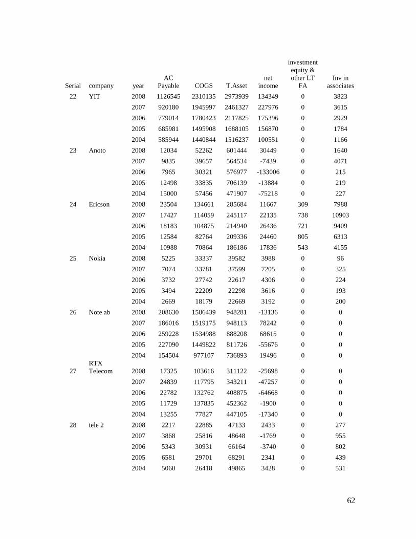
62

Serial company year AC

Payable COGS T.Asset net

income

investment equity & other LT

FA Inv in

associates

22 YIT 2008 1126545 2310135 2973939 134349 0 3823

2007 920180 1945997 2461327 227976 0 3615

2006 779014 1780423 2117825 175396 0 2929

2005 685981 1495908 1688105 156870 0 1784

2004 585944 1440844 1516237 100551 0 1166

23 Anoto 2008 12034 52262 601444 30449 0 1640

2007 9835 39657 564534 -7439 0 4071

2006 7965 30321 576977 -133006 0 215

2005 12498 33835 706139 -13884 0 219

2004 15000 57456 471907 -75218 0 227

24 Ericson 2008 23504 134661 285684 11667 309 7988

2007 17427 114059 245117 22135 738 10903

2006 18183 104875 214940 26436 721 9409

2005 12584 82764 209336 24460 805 6313

2004 10988 70864 186186 17836 543 4155

25 Nokia 2008 5225 33337 39582 3988 0 96

2007 7074 33781 37599 7205 0 325

2006 3732 27742 22617 4306 0 224

2005 3494 22209 22298 3616 0 193

2004 2669 18179 22669 3192 0 200

26 Note ab 2008 208630 1586439 948281 -13136 0 0

2007 186016 1519175 948113 78242 0 0

2006 259228 1534988 888208 68615 0 0

2005 227090 1449822 811726 -55676 0 0

2004 154504 977107 736893 19496 0 0

27 RTX Telecom 2008 17325 103616 311122 -25698 0 0

2007 24839 117795 343211 -47257 0 0

2006 22782 132762 408875 -64668 0 0

2005 11729 137835 452362 -1900 0 0

2004 13255 77827 447105 -17340 0 0

28 tele 2 2008 2217 22885 47133 2433 0 277

2007 3868 25816 48648 -1769 0 955

2006 5343 30931 66164 -3740 0 802

2005 6581 29701 68291 2341 0 439

2004 5060 26418 49865 3428 0 531

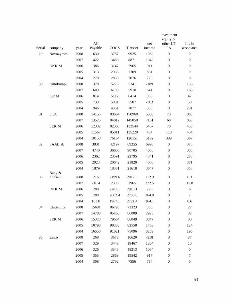
63

Serial company year AC

Payable COGS T.Asset net

income

investment equity & other LT

FA Inv in

associates

29 Novozymes 2008 630 3787 9925 1062 0 0

2007 422 3489 8871 1042 0 0

DKK M 2006 386 3147 7965 911 0 0

2005 313 2936 7309 861 0 0

2004 270 2838 7076 775 0 0

30 Outokumpu 2008 378 5276 5341 -189 0 156

2007 609 6108 5910 641 0 163

Eur M 2006 814 5112 6414 963 0 47

2005 739 5081 5507 -363 0 50

2004 946 4361 7077 386 0 291

31 SCA 2008 14156 89684 158968 5598 73 983

2007 13526 84812 145050 7161 68 950

SEK M 2006 12332 82368 133544 5467 79 439

2005 11567 85811 135220 454 119 454

2004 10150 76164 126151 5192 309 387

32 SAAB ab 2008 3831 42197 69255 6998 0 373

2007 4740 36606 90705 4658 0 353

2006 2362 23591 22795 4341 0 283

2005 2023 20642 21820 4068 0 381

2004 1879 18381 21618 3647 0 358

33 Bang & olufsen 2008 216 2199.6 2817.3 112.3 0 6.3

2007 216.4 2338 2965 372.5 0 15.8

DKK M 2006 208 2281.1 2915.1 296 0 6

2005 208 2002.4 2783.8 264.9 0 7

2004 183.8 1967.1 2721.4 264.1 0 8.6

34 Electrolux 2008 15681 86795 73323 366 0 27

2007 14788 85466 66089 2925 0 32

SEK M 2006 15320 79664 66049 3847 0 80

2005 18798 98358 82558 1763 0 124

2004 16550 91021 75096 3259 0 196

35 Eniro 2008 268 3673 16620 -318 0 37

2007 329 3443 18467 1304 0 10

2006 326 3545 18213 1054 0 0

2005 355 2863 19542 917 0 7

2004 308 2792 7356 764 0 0

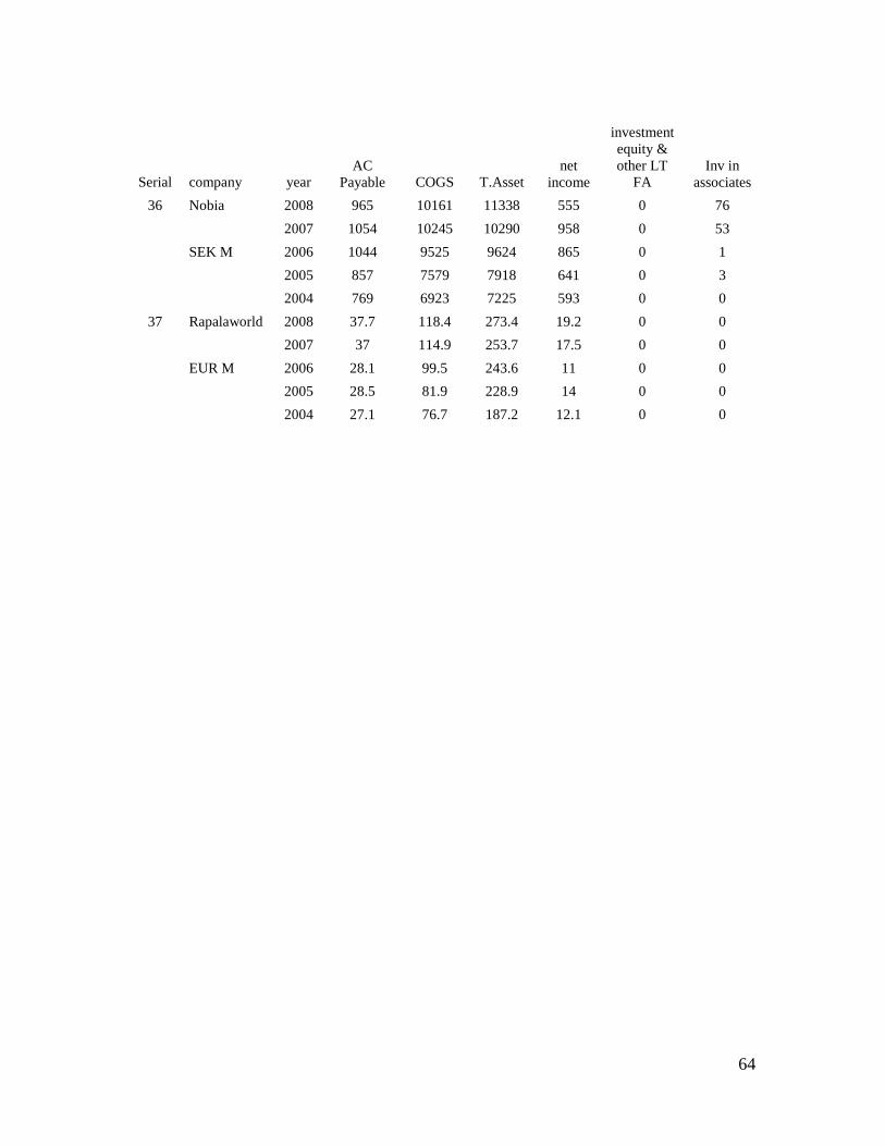
64

Serial company year AC

Payable COGS T.Asset net

income

investment equity & other LT

FA Inv in

associates

36 Nobia 2008 965 10161 11338 555 0 76

2007 1054 10245 10290 958 0 53

SEK M 2006 1044 9525 9624 865 0 1

2005 857 7579 7918 641 0 3

2004 769 6923 7225 593 0 0

37 Rapalaworld 2008 37.7 118.4 273.4 19.2 0 0

2007 37 114.9 253.7 17.5 0 0

EUR M 2006 28.1 99.5 243.6 11 0 0

2005 28.5 81.9 228.9 14 0 0

2004 27.1 76.7 187.2 12.1 0 0

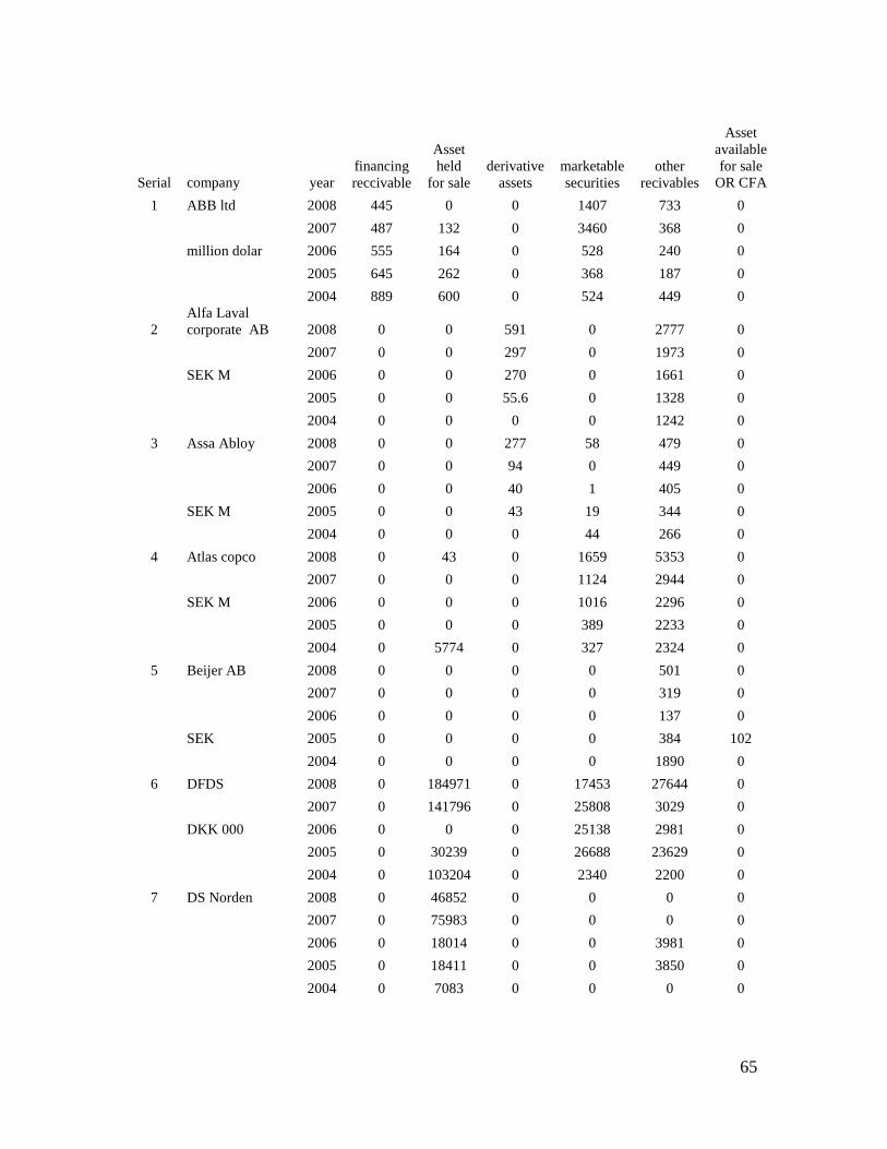
65

Serial company year financing reccivable

Asset held

for sale derivative

assets marketable securities

other recivables

Asset available for sale

OR CFA

1 ABB ltd 2008 445 0 0 1407 733 0

2007 487 132 0 3460 368 0

million dolar 2006 555 164 0 528 240 0

2005 645 262 0 368 187 0

2004 889 600 0 524 449 0

2 Alfa Laval corporate AB 2008 0 0 591 0 2777 0

2007 0 0 297 0 1973 0

SEK M 2006 0 0 270 0 1661 0

2005 0 0 55.6 0 1328 0

2004 0 0 0 0 1242 0

3 Assa Abloy 2008 0 0 277 58 479 0

2007 0 0 94 0 449 0

2006 0 0 40 1 405 0

SEK M 2005 0 0 43 19 344 0

2004 0 0 0 44 266 0

4 Atlas copco 2008 0 43 0 1659 5353 0

2007 0 0 0 1124 2944 0

SEK M 2006 0 0 0 1016 2296 0

2005 0 0 0 389 2233 0

2004 0 5774 0 327 2324 0

5 Beijer AB 2008 0 0 0 0 501 0

2007 0 0 0 0 319 0

2006 0 0 0 0 137 0

SEK 2005 0 0 0 0 384 102

2004 0 0 0 0 1890 0

6 DFDS 2008 0 184971 0 17453 27644 0

2007 0 141796 0 25808 3029 0

DKK 000 2006 0 0 0 25138 2981 0

2005 0 30239 0 26688 23629 0

2004 0 103204 0 2340 2200 0

7 DS Norden 2008 0 46852 0 0 0 0

2007 0 75983 0 0 0 0

2006 0 18014 0 0 3981 0

2005 0 18411 0 0 3850 0

2004 0 7083 0 0 0 0

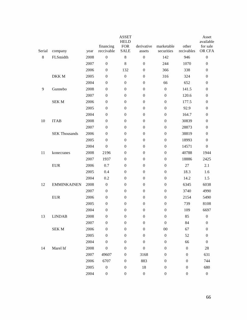
66

Serial company year financing reccivable

ASSET HELD FOR SALE

derivative assets

marketable securities

other recivables

Asset available for sale

OR CFA

8 FLSmidth 2008 0 8 0 142 946 0

2007 0 8 0 244 1070 0

2006 0 132 0 366 338 0

DKK M 2005 0 0 0 316 324 0

2004 0 0 0 66 652 0

9 Gunnebo 2008 0 0 0 0 141.5 0

2007 0 0 0 0 120.6 0

SEK M 2006 0 0 0 0 177.5 0

2005 0 0 0 0 92.9 0

2004 0 0 0 0 164.7 0

10 ITAB 2008 0 0 0 0 30839 0

2007 0 0 0 0 28873 0

SEK Thousands 2006 0 0 0 0 38819 0

2005 0 0 0 0 18993 0

2004 0 0 0 0 14571 0

11 konecranes 2008 2196 0 0 0 40788 1944

2007 1937 0 0 0 18886 2425

EUR 2006 0.7 0 0 0 27 2.1

2005 0.4 0 0 0 18.3 1.6

2004 0.2 0 0 0 14.2 1.5

12 EMMINKAINEN 2008 0 0 0 0 6345 6038

2007 0 0 0 0 3740 4990

EUR 2006 0 0 0 0 2154 5490

2005 0 0 0 0 739 8108

2004 0 0 0 0 109 6697

13 LINDAB 2008 0 0 0 0 85 0

2007 0 0 0 0 84 0

SEK M 2006 0 0 0 00 67 0

2005 0 0 0 0 52 0

2004 0 0 0 0 66 0

14 Marel hf 2008 0 0 0 0 0 28

2007 49607 0 3168 0 0 631

2006 6707 0 883 0 0 744

2005 0 0 18 0 0 680

2004 0 0 0 0 0 0

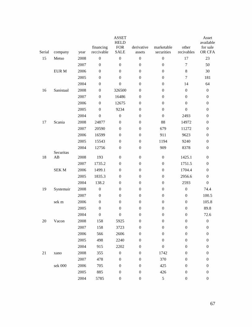
67

Serial company year financing reccivable

ASSET HELD FOR SALE

derivative assets

marketable securities

other recivables

Asset available for sale

OR CFA

15 Metso 2008 0 0 0 0 17 23

2007 0 0 0 0 7 50

EUR M 2006 0 0 0 0 8 30

2005 0 0 0 0 7 181

2004 0 0 0 0 14 64

16 Sanistaal 2008 0 326500 0 0 0 0

2007 0 16486 0 0 0 0

2006 0 12675 0 0 0 0

2005 0 9234 0 0 0 0

2004 0 0 0 0 2493 0

17 Scania 2008 24877 0 0 88 14972 0

2007 20590 0 0 679 11272 0

2006 16599 0 0 911 9623 0

2005 15543 0 0 1194 9240 0

2004 12756 0 0 909 8378 0

18 Securitas AB 2008 193 0 0 0 1425.1 0

2007 1735.2 0 0 0 1751.5 0

SEK M 2006 1499.1 0 0 0 1704.4 0

2005 1835.3 0 0 0 2956.6 0

2004 138.2 0 0 0 2593 0

19 Systemair 2008 0 0 0 0 0 74.4

2007 0 0 0 0 0 100.5

sek m 2006 0 0 0 0 0 105.8

2005 0 0 0 0 0 89.8

2004 0 0 0 0 0 72.6

20 Vacon 2008 158 5925 0 0 0 0

2007 158 3723 0 0 0 0

2006 566 2606 0 0 0 0

2005 498 2240 0 0 0 0

2004 915 2202 0 0 0 0

21 xano 2008 355 0 0 1742 0 0

2007 478 0 0 370 0 0

sek 000 2006 705 0 0 425 0 0

2005 885 0 0 426 0 0

2004 5785 0 0 5 0 0

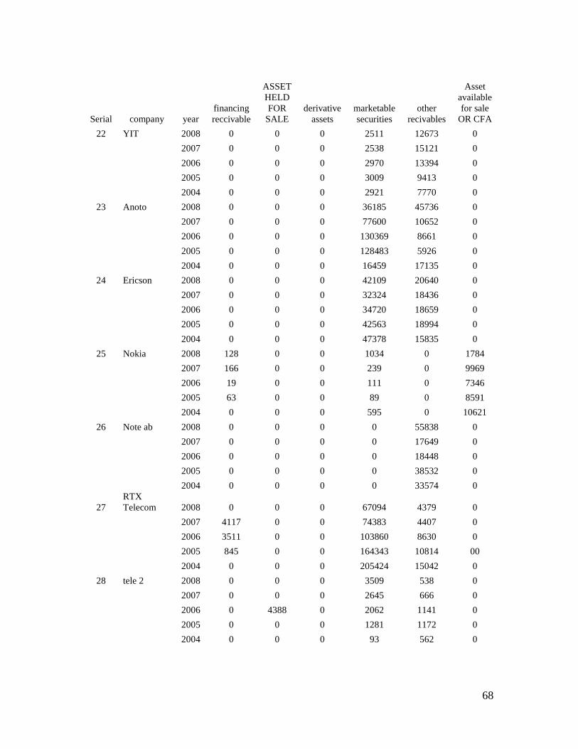
68

Serial company year financing reccivable

ASSET HELD FOR SALE

derivative assets

marketable securities

other recivables

Asset available for sale

OR CFA

22 YIT 2008 0 0 0 2511 12673 0

2007 0 0 0 2538 15121 0

2006 0 0 0 2970 13394 0

2005 0 0 0 3009 9413 0

2004 0 0 0 2921 7770 0

23 Anoto 2008 0 0 0 36185 45736 0

2007 0 0 0 77600 10652 0

2006 0 0 0 130369 8661 0

2005 0 0 0 128483 5926 0

2004 0 0 0 16459 17135 0

24 Ericson 2008 0 0 0 42109 20640 0

2007 0 0 0 32324 18436 0

2006 0 0 0 34720 18659 0

2005 0 0 0 42563 18994 0

2004 0 0 0 47378 15835 0

25 Nokia 2008 128 0 0 1034 0 1784

2007 166 0 0 239 0 9969

2006 19 0 0 111 0 7346

2005 63 0 0 89 0 8591

2004 0 0 0 595 0 10621

26 Note ab 2008 0 0 0 0 55838 0

2007 0 0 0 0 17649 0

2006 0 0 0 0 18448 0

2005 0 0 0 0 38532 0

2004 0 0 0 0 33574 0

27 RTX Telecom 2008 0 0 0 67094 4379 0

2007 4117 0 0 74383 4407 0

2006 3511 0 0 103860 8630 0

2005 845 0 0 164343 10814 00

2004 0 0 0 205424 15042 0

28 tele 2 2008 0 0 0 3509 538 0

2007 0 0 0 2645 666 0

2006 0 4388 0 2062 1141 0

2005 0 0 0 1281 1172 0

2004 0 0 0 93 562 0

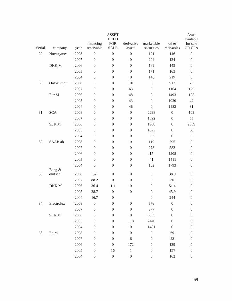
69

Serial company year financing reccivable

ASSET HELD FOR SALE

derivative assets

marketable securities

other recivables

Asset available for sale

OR CFA

29 Novozymes 2008 0 0 0 191 146 0

2007 0 0 0 204 124 0

DKK M 2006 0 0 0 189 145 0

2005 0 0 0 171 163 0

2004 0 0 0 146 219 0

30 Outokumpu 2008 0 0 101 0 913 75

2007 0 0 63 0 1164 129

Eur M 2006 0 0 48 0 1493 188

2005 0 0 43 0 1020 42

2004 0 0 46 0 1482 61

31 SCA 2008 0 0 0 2298 0 102

2007 0 0 0 1892 0 55

SEK M 2006 0 0 0 1960 0 2559

2005 0 0 0 1822 0 68

2004 0 0 0 836 0 0

32 SAAB ab 2008 0 0 0 119 795 0

2007 0 0 0 273 582 0

2006 0 0 0 15 1208 0

2005 0 0 0 41 1411 0

2004 0 0 0 102 1793 0

33 Bang & olufsen 2008 52 0 0 0 38.9 0

2007 88.2 0 0 0 30 0

DKK M 2006 36.4 1.1 0 0 51.4 0

2005 28.7 0 0 0 45.9 0

2004 16.7 0 0 244 0

34 Electrolux 2008 0 0 0 576 0 0

2007 0 0 0 877 0 0

SEK M 2006 0 0 0 3335 0 0

2005 0 0 118 2440 0 0

2004 0 0 0 1481 0 0

35 Eniro 2008 0 0 0 0 69 0

2007 0 0 6 0 23 0

2006 0 0 172 0 129 0

2005 0 16 1 0 157 0

2004 0 0 0 0 162 0

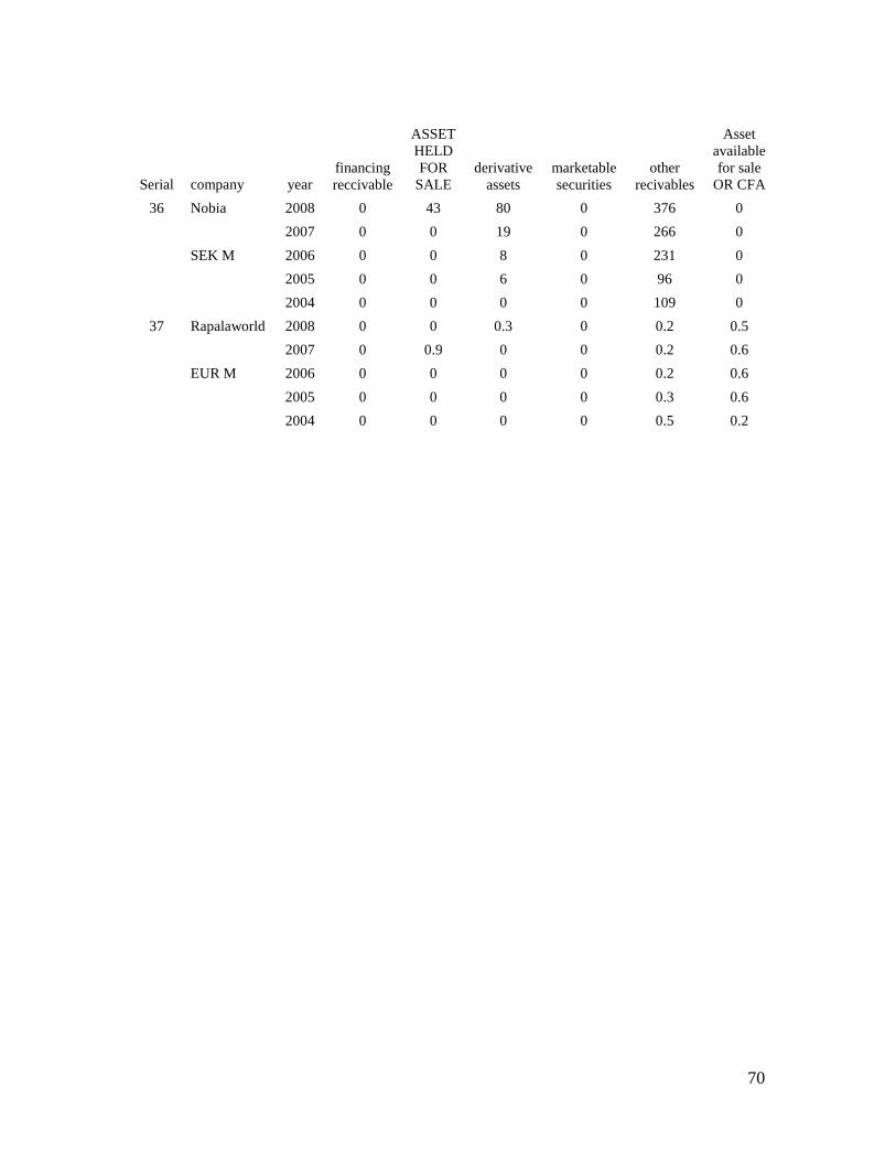
70

Serial company year financing reccivable

ASSET HELD FOR SALE

derivative assets

marketable securities

other recivables

Asset available for sale

OR CFA

36 Nobia 2008 0 43 80 0 376 0

2007 0 0 19 0 266 0

SEK M 2006 0 0 8 0 231 0

2005 0 0 6 0 96 0

2004 0 0 0 0 109 0

37 Rapalaworld 2008 0 0 0.3 0 0.2 0.5

2007 0 0.9 0 0 0.2 0.6

EUR M 2006 0 0 0 0 0.2 0.6

2005 0 0 0 0 0.3 0.6

2004 0 0 0 0 0.5 0.2

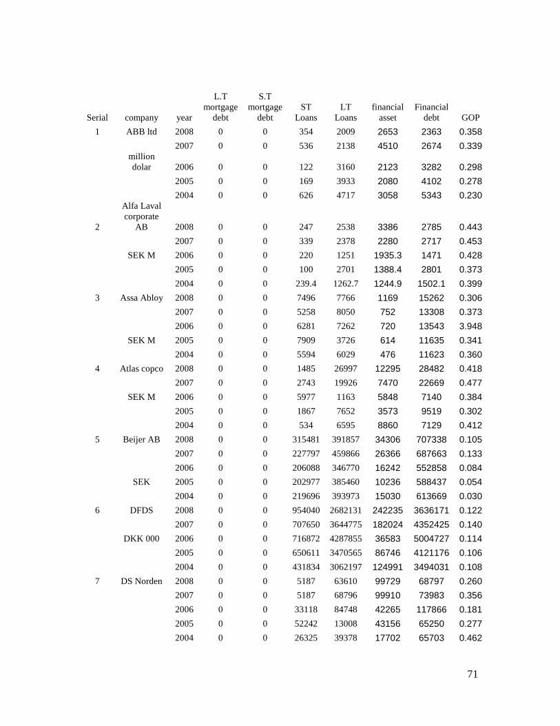
71

Serial company year

L.T mortgage

debt

S.T mortgage

debt ST

Loans LT

Loans financial

asset Financial

debt GOP

1 ABB ltd 2008 0 0 354 2009 2653 2363 0.358

2007 0 0 536 2138 4510 2674 0.339

million dolar 2006 0 0 122 3160 2123 3282 0.298

2005 0 0 169 3933 2080 4102 0.278

2004 0 0 626 4717 3058 5343 0.230

2

Alfa Laval corporate

AB 2008 0 0 247 2538 3386 2785 0.443

2007 0 0 339 2378 2280 2717 0.453

SEK M 2006 0 0 220 1251 1935.3 1471 0.428

2005 0 0 100 2701 1388.4 2801 0.373

2004 0 0 239.4 1262.7 1244.9 1502.1 0.399

3 Assa Abloy 2008 0 0 7496 7766 1169 15262 0.306

2007 0 0 5258 8050 752 13308 0.373

2006 0 0 6281 7262 720 13543 3.948

SEK M 2005 0 0 7909 3726 614 11635 0.341

2004 0 0 5594 6029 476 11623 0.360

4 Atlas copco 2008 0 0 1485 26997 12295 28482 0.418

2007 0 0 2743 19926 7470 22669 0.477

SEK M 2006 0 0 5977 1163 5848 7140 0.384

2005 0 0 1867 7652 3573 9519 0.302

2004 0 0 534 6595 8860 7129 0.412

5 Beijer AB 2008 0 0 315481 391857 34306 707338 0.105

2007 0 0 227797 459866 26366 687663 0.133

2006 0 0 206088 346770 16242 552858 0.084

SEK 2005 0 0 202977 385460 10236 588437 0.054

2004 0 0 219696 393973 15030 613669 0.030

6 DFDS 2008 0 0 954040 2682131 242235 3636171 0.122

2007 0 0 707650 3644775 182024 4352425 0.140

DKK 000 2006 0 0 716872 4287855 36583 5004727 0.114

2005 0 0 650611 3470565 86746 4121176 0.106

2004 0 0 431834 3062197 124991 3494031 0.108

7 DS Norden 2008 0 0 5187 63610 99729 68797 0.260

2007 0 0 5187 68796 99910 73983 0.356

2006 0 0 33118 84748 42265 117866 0.181

2005 0 0 52242 13008 43156 65250 0.277

2004 0 0 26325 39378 17702 65703 0.462

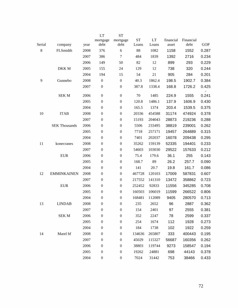
72

Serial company year

LT mortgage

debt

ST mortgage

debt ST

Loans LT

Loans financial

asset Financial

debt GOP

8 FLSmidth 2008 376 6 88 1082 1158 1552 0.287

2007 386 7 484 1839 1392 2716 0.234

2006 149 50 82 12 899 293 0.229

DKK M 2005 155 24 129 12 738 320 0.244

2004 194 15 54 21 905 284 0.201

9 Gunnebo 2008 0 0 40.3 1862.4 198.5 1902.7 0.384

2007 0 0 387.8 1338.4 168.8 1726.2 0.425

SEK M 2006 0 0 70 1485 224.9 1555 -

0.241

2005 0 0 120.8 1486.1 137.9 1606.9 0.430

2004 0 0 165.5 1374 203.4 1539.5 0.375

10 ITAB 2008 0 0 20336 454588 31174 474924 0.378

2007 0 0 15193 204043 28873 219236 0.288

SEK Thousands 2006 0 0 5506 233495 38819 239001 0.262

2005 0 0 7718 257171 19457 264889 0.315

2004 0 0 7401 202037 16078 209438 0.295

11 konecranes 2008 0 0 35262 159139 52335 194401 0.233

2007 0 0 54603 103030 29522 157633 0.212

EUR 2006 0 0 75.4 179.6 36.1 255 0.143

2005 0 0 168.7 89 26.2 257.7 0.090

2004 0 0 141 20.7 19.8 161.7 0.086

12 EMMINKAINEN 2008 0 0 467728 120103 17009 587831 0.607

2007 0 0 217552 141310 13472 358862 0.723

EUR 2006 0 0 252452 92833 11556 345285 0.708

2005 0 0 160503 106019 11599 266522 0.806

2004 0 0 168481 112089 9405 280570 0.713

13 LINDAB 2008 0 0 235 2652 96 2887 0.362

2007 0 0 154 2401 97 2555 0.381

SEK M 2006 0 0 352 2247 78 2599 0.337

2005 0 0 254 1674 112 1928 0.273

2004 0 0 184 1738 102 1922 0.259

14 Marel hf 2008 0 0 134636 265807 333 400443 0.195

2007 0 0 45029 115327 56687 160356 0.262

2006 0 0 38803 119744 9273 158547 0.194

2005 0 0 19262 24881 698 44143 0.378

2004 0 0 7024 31442 753 38466 0.433

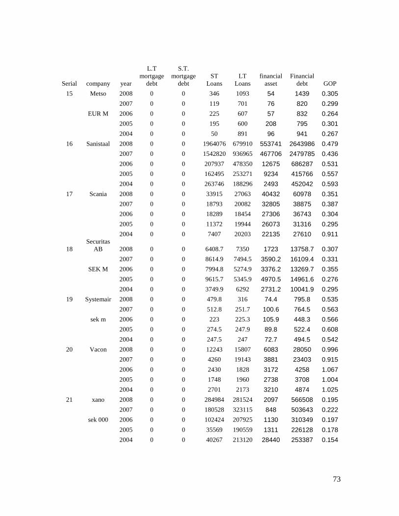
73

Serial company year

L.T mortgage

debt

S.T. mortgage

debt ST

Loans LT

Loans financial

asset Financial

debt GOP

15 Metso 2008 0 0 346 1093 54 1439 0.305

2007 0 0 119 701 76 820 0.299

EUR M 2006 0 0 225 607 57 832 0.264

2005 0 0 195 600 208 795 0.301

2004 0 0 50 891 96 941 0.267

16 Sanistaal 2008 0 0 1964076 679910 553741 2643986 0.479

2007 0 0 1542820 936965 467706 2479785 0.436

2006 0 0 207937 478350 12675 686287 0.531

2005 0 0 162495 253271 9234 415766 0.557

2004 0 0 263746 188296 2493 452042 0.593

17 Scania 2008 0 0 33915 27063 40432 60978 0.351

2007 0 0 18793 20082 32805 38875 0.387

2006 0 0 18289 18454 27306 36743 0.304

2005 0 0 11372 19944 26073 31316 0.295

2004 0 0 7407 20203 22135 27610 0.911

18 Securitas

AB 2008 0 0 6408.7 7350 1723 13758.7 0.307

2007 0 0 8614.9 7494.5 3590.2 16109.4 0.331

SEK M 2006 0 0 7994.8 5274.9 3376.2 13269.7 0.355

2005 0 0 9615.7 5345.9 4970.5 14961.6 0.276

2004 0 0 3749.9 6292 2731.2 10041.9 0.295

19 Systemair 2008 0 0 479.8 316 74.4 795.8 0.535

2007 0 0 512.8 251.7 100.6 764.5 0.563

sek m 2006 0 0 223 225.3 105.9 448.3 0.566

2005 0 0 274.5 247.9 89.8 522.4 0.608

2004 0 0 247.5 247 72.7 494.5 0.542

20 Vacon 2008 0 0 12243 15807 6083 28050 0.996

2007 0 0 4260 19143 3881 23403 0.915

2006 0 0 2430 1828 3172 4258 1.067

2005 0 0 1748 1960 2738 3708 1.004

2004 0 0 2701 2173 3210 4874 1.025

21 xano 2008 0 0 284984 281524 2097 566508 0.195

2007 0 0 180528 323115 848 503643 0.222

sek 000 2006 0 0 102424 207925 1130 310349 0.197

2005 0 0 35569 190559 1311 226128 0.178

2004 0 0 40267 213120 28440 253387 0.154

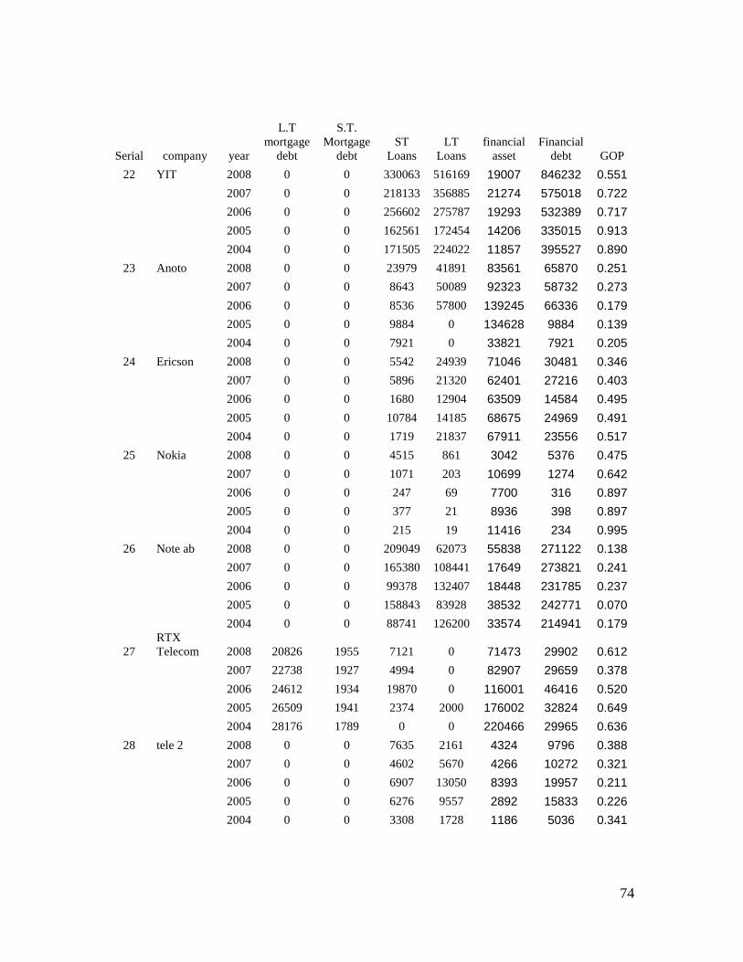
74

Serial company year

L.T mortgage

debt

S.T. Mortgage

debt ST

Loans LT

Loans financial

asset Financial

debt GOP

22 YIT 2008 0 0 330063 516169 19007 846232 0.551

2007 0 0 218133 356885 21274 575018 0.722

2006 0 0 256602 275787 19293 532389 0.717

2005 0 0 162561 172454 14206 335015 0.913

2004 0 0 171505 224022 11857 395527 0.890

23 Anoto 2008 0 0 23979 41891 83561 65870 0.251

2007 0 0 8643 50089 92323 58732 0.273

2006 0 0 8536 57800 139245 66336 0.179

2005 0 0 9884 0 134628 9884 0.139

2004 0 0 7921 0 33821 7921 0.205

24 Ericson 2008 0 0 5542 24939 71046 30481 0.346

2007 0 0 5896 21320 62401 27216 0.403

2006 0 0 1680 12904 63509 14584 0.495

2005 0 0 10784 14185 68675 24969 0.491

2004 0 0 1719 21837 67911 23556 0.517

25 Nokia 2008 0 0 4515 861 3042 5376 0.475

2007 0 0 1071 203 10699 1274 0.642

2006 0 0 247 69 7700 316 0.897

2005 0 0 377 21 8936 398 0.897

2004 0 0 215 19 11416 234 0.995

26 Note ab 2008 0 0 209049 62073 55838 271122 0.138

2007 0 0 165380 108441 17649 273821 0.241

2006 0 0 99378 132407 18448 231785 0.237

2005 0 0 158843 83928 38532 242771 0.070

2004 0 0 88741 126200 33574 214941 0.179

27 RTX Telecom 2008 20826 1955 7121 0 71473 29902 0.612

2007 22738 1927 4994 0 82907 29659 0.378

2006 24612 1934 19870 0 116001 46416 0.520

2005 26509 1941 2374 2000 176002 32824 0.649

2004 28176 1789 0 0 220466 29965 0.636

28 tele 2 2008 0 0 7635 2161 4324 9796 0.388

2007 0 0 4602 5670 4266 10272 0.321

2006 0 0 6907 13050 8393 19957 0.211

2005 0 0 6276 9557 2892 15833 0.226

2004 0 0 3308 1728 1186 5036 0.341

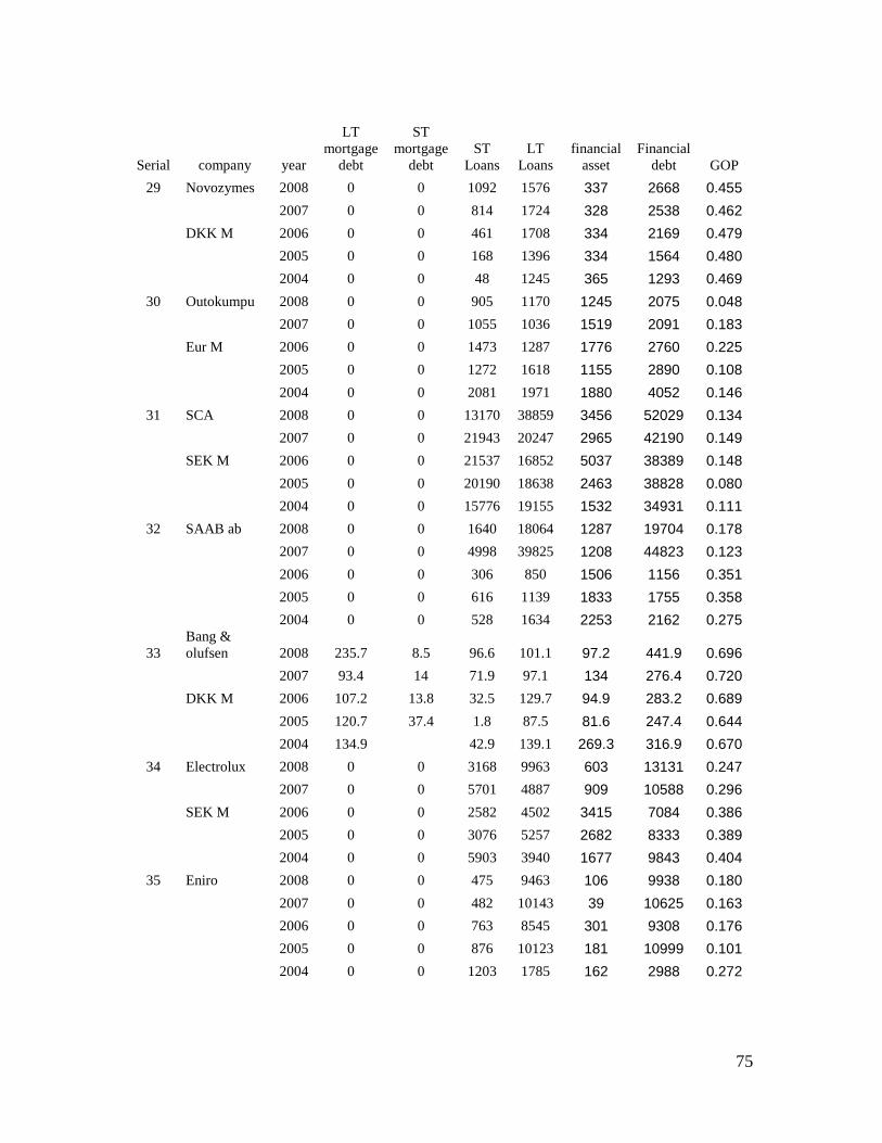
75

Serial company year

LT mortgage

debt

ST mortgage

debt ST

Loans LT

Loans financial

asset Financial

debt GOP

29 Novozymes 2008 0 0 1092 1576 337 2668 0.455

2007 0 0 814 1724 328 2538 0.462

DKK M 2006 0 0 461 1708 334 2169 0.479

2005 0 0 168 1396 334 1564 0.480

2004 0 0 48 1245 365 1293 0.469

30 Outokumpu 2008 0 0 905 1170 1245 2075 0.048

2007 0 0 1055 1036 1519 2091 0.183

Eur M 2006 0 0 1473 1287 1776 2760 0.225

2005 0 0 1272 1618 1155 2890 0.108

2004 0 0 2081 1971 1880 4052 0.146

31 SCA 2008 0 0 13170 38859 3456 52029 0.134

2007 0 0 21943 20247 2965 42190 0.149

SEK M 2006 0 0 21537 16852 5037 38389 0.148

2005 0 0 20190 18638 2463 38828 0.080

2004 0 0 15776 19155 1532 34931 0.111

32 SAAB ab 2008 0 0 1640 18064 1287 19704 0.178

2007 0 0 4998 39825 1208 44823 0.123

2006 0 0 306 850 1506 1156 0.351

2005 0 0 616 1139 1833 1755 0.358

2004 0 0 528 1634 2253 2162 0.275

33 Bang & olufsen 2008 235.7 8.5 96.6 101.1 97.2 441.9 0.696

2007 93.4 14 71.9 97.1 134 276.4 0.720

DKK M 2006 107.2 13.8 32.5 129.7 94.9 283.2 0.689

2005 120.7 37.4 1.8 87.5 81.6 247.4 0.644

2004 134.9 42.9 139.1 269.3 316.9 0.670

34 Electrolux 2008 0 0 3168 9963 603 13131 0.247

2007 0 0 5701 4887 909 10588 0.296

SEK M 2006 0 0 2582 4502 3415 7084 0.386

2005 0 0 3076 5257 2682 8333 0.389

2004 0 0 5903 3940 1677 9843 0.404

35 Eniro 2008 0 0 475 9463 106 9938 0.180

2007 0 0 482 10143 39 10625 0.163

2006 0 0 763 8545 301 9308 0.176

2005 0 0 876 10123 181 10999 0.101

2004 0 0 1203 1785 162 2988 0.272

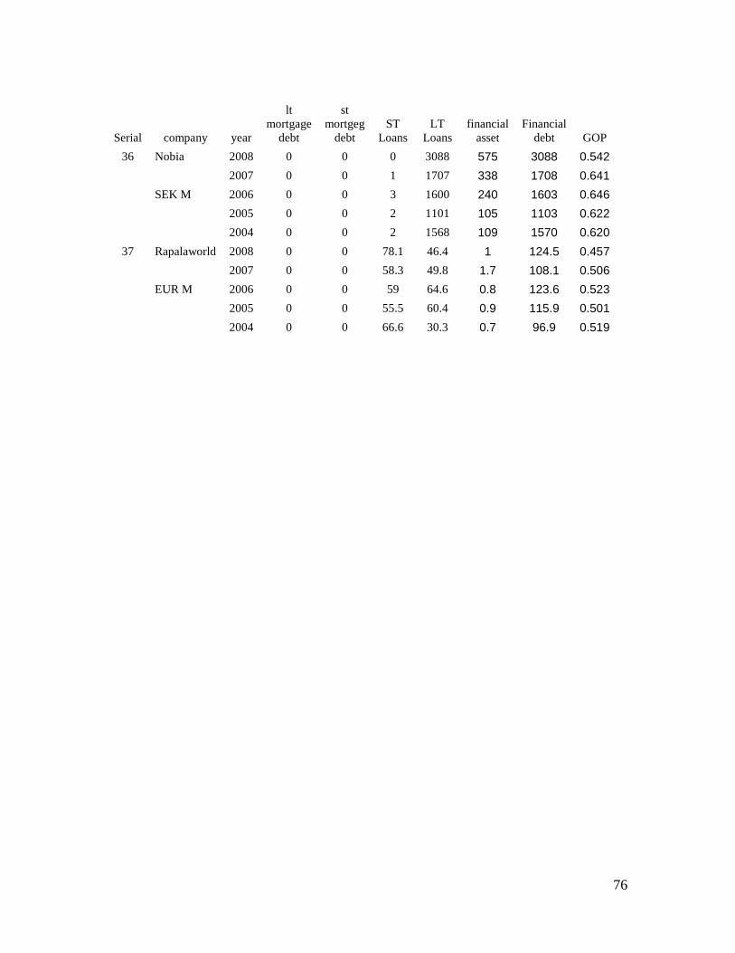
76

Serial company year

lt mortgage

debt

st mortgeg

debt ST

Loans LT

Loans financial

asset Financial

debt GOP

36 Nobia 2008 0 0 0 3088 575 3088 0.542

2007 0 0 1 1707 338 1708 0.641

SEK M 2006 0 0 3 1600 240 1603 0.646

2005 0 0 2 1101 105 1103 0.622

2004 0 0 2 1568 109 1570 0.620

37 Rapalaworld 2008 0 0 78.1 46.4 1 124.5 0.457

2007 0 0 58.3 49.8 1.7 108.1 0.506

EUR M 2006 0 0 59 64.6 0.8 123.6 0.523

2005 0 0 55.5 60.4 0.9 115.9 0.501

2004 0 0 66.6 30.3 0.7 96.9 0.519

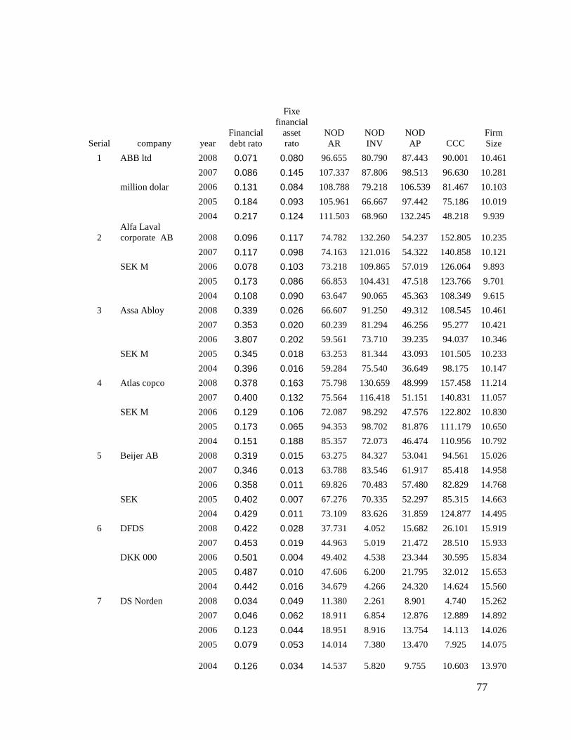
77

Serial company year Financial debt rato

Fixe financial

asset rato

NOD AR

NOD INV

NOD AP CCC

Firm Size

1 ABB ltd 2008 0.071 0.080 96.655 80.790 87.443 90.001 10.461

2007 0.086 0.145 107.337 87.806 98.513 96.630 10.281

million dolar 2006 0.131 0.084 108.788 79.218 106.539 81.467 10.103

2005 0.184 0.093 105.961 66.667 97.442 75.186 10.019

2004 0.217 0.124 111.503 68.960 132.245 48.218 9.939

2 Alfa Laval corporate AB 2008 0.096 0.117 74.782 132.260 54.237 152.805 10.235

2007 0.117 0.098 74.163 121.016 54.322 140.858 10.121

SEK M 2006 0.078 0.103 73.218 109.865 57.019 126.064 9.893

2005 0.173 0.086 66.853 104.431 47.518 123.766 9.701

2004 0.108 0.090 63.647 90.065 45.363 108.349 9.615

3 Assa Abloy 2008 0.339 0.026 66.607 91.250 49.312 108.545 10.461

2007 0.353 0.020 60.239 81.294 46.256 95.277 10.421

2006 3.807 0.202 59.561 73.710 39.235 94.037 10.346

SEK M 2005 0.345 0.018 63.253 81.344 43.093 101.505 10.233

2004 0.396 0.016 59.284 75.540 36.649 98.175 10.147

4 Atlas copco 2008 0.378 0.163 75.798 130.659 48.999 157.458 11.214

2007 0.400 0.132 75.564 116.418 51.151 140.831 11.057

SEK M 2006 0.129 0.106 72.087 98.292 47.576 122.802 10.830

2005 0.173 0.065 94.353 98.702 81.876 111.179 10.650

2004 0.151 0.188 85.357 72.073 46.474 110.956 10.792

5 Beijer AB 2008 0.319 0.015 63.275 84.327 53.041 94.561 15.026

2007 0.346 0.013 63.788 83.546 61.917 85.418 14.958

2006 0.358 0.011 69.826 70.483 57.480 82.829 14.768

SEK 2005 0.402 0.007 67.276 70.335 52.297 85.315 14.663

2004 0.429 0.011 73.109 83.626 31.859 124.877 14.495

6 DFDS 2008 0.422 0.028 37.731 4.052 15.682 26.101 15.919

2007 0.453 0.019 44.963 5.019 21.472 28.510 15.933

DKK 000 2006 0.501 0.004 49.402 4.538 23.344 30.595 15.834

2005 0.487 0.010 47.606 6.200 21.795 32.012 15.653

2004 0.442 0.016 34.679 4.266 24.320 14.624 15.560

7 DS Norden 2008 0.034 0.049 11.380 2.261 8.901 4.740 15.262

2007 0.046 0.062 18.911 6.854 12.876 12.889 14.892

2006 0.123 0.044 18.951 8.916 13.754 14.113 14.026

2005 0.079 0.053 14.014 7.380 13.470 7.925 14.075

2004 0.126 0.034 14.537

5.820 9.755 10.603 13.970

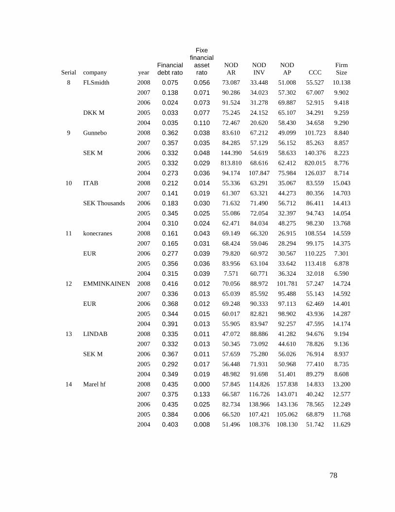
78

Serial company year Financial debt rato

Fixe financial

asset rato

NOD AR

NOD INV

NOD AP CCC

Firm Size

8 FLSmidth 2008 0.075 0.056 73.087 33.448 51.008 55.527 10.138

2007 0.138 0.071 90.286 34.023 57.302 67.007 9.902

2006 0.024 0.073 91.524 31.278 69.887 52.915 9.418

DKK M 2005 0.033 0.077 75.245 24.152 65.107 34.291 9.259

2004 0.035 0.110 72.467 20.620 58.430 34.658 9.290

9 Gunnebo 2008 0.362 0.038 83.610 67.212 49.099 101.723 8.840

2007 0.357 0.035 84.285 57.129 56.152 85.263 8.857

SEK M 2006 0.332 0.048 144.390 54.619 58.633 140.376 8.223

2005 0.332 0.029 813.810 68.616 62.412 820.015 8.776

2004 0.273 0.036 94.174 107.847 75.984 126.037 8.714

10 ITAB 2008 0.212 0.014 55.336 63.291 35.067 83.559 15.043

2007 0.141 0.019 61.307 63.321 44.273 80.356 14.703

SEK Thousands 2006 0.183 0.030 71.632 71.490 56.712 86.411 14.413

2005 0.345 0.025 55.086 72.054 32.397 94.743 14.054

2004 0.310 0.024 62.471 84.034 48.275 98.230 13.768

11 konecranes 2008 0.161 0.043 69.149 66.320 26.915 108.554 14.559

2007 0.165 0.031 68.424 59.046 28.294 99.175 14.375

EUR 2006 0.277 0.039 79.820 60.972 30.567 110.225 7.301

2005 0.356 0.036 83.956 63.104 33.642 113.418 6.878

2004 0.315 0.039 7.571 60.771 36.324 32.018 6.590

12 EMMINKAINEN 2008 0.416 0.012 70.056 88.972 101.781 57.247 14.724

2007 0.336 0.013 65.039 85.592 95.488 55.143 14.592

EUR 2006 0.368 0.012 69.248 90.333 97.113 62.469 14.401

2005 0.344 0.015 60.017 82.821 98.902 43.936 14.287

2004 0.391 0.013 55.905 83.947 92.257 47.595 14.174

13 LINDAB 2008 0.335 0.011 47.072 88.886 41.282 94.676 9.194

2007 0.332 0.013 50.345 73.092 44.610 78.826 9.136

SEK M 2006 0.367 0.011 57.659 75.280 56.026 76.914 8.937

2005 0.292 0.017 56.448 71.931 50.968 77.410 8.735

2004 0.349 0.019 48.982 91.698 51.401 89.279 8.608

14 Marel hf 2008 0.435 0.000 57.845 114.826 157.838 14.833 13.200

2007 0.375 0.133 66.587 116.726 143.071 40.242 12.577

2006 0.435 0.025 82.734 138.966 143.136 78.565 12.249

2005 0.384 0.006 66.520 107.421 105.062 68.879 11.768

2004 0.403 0.008 51.496 108.376 108.130 51.742 11.629

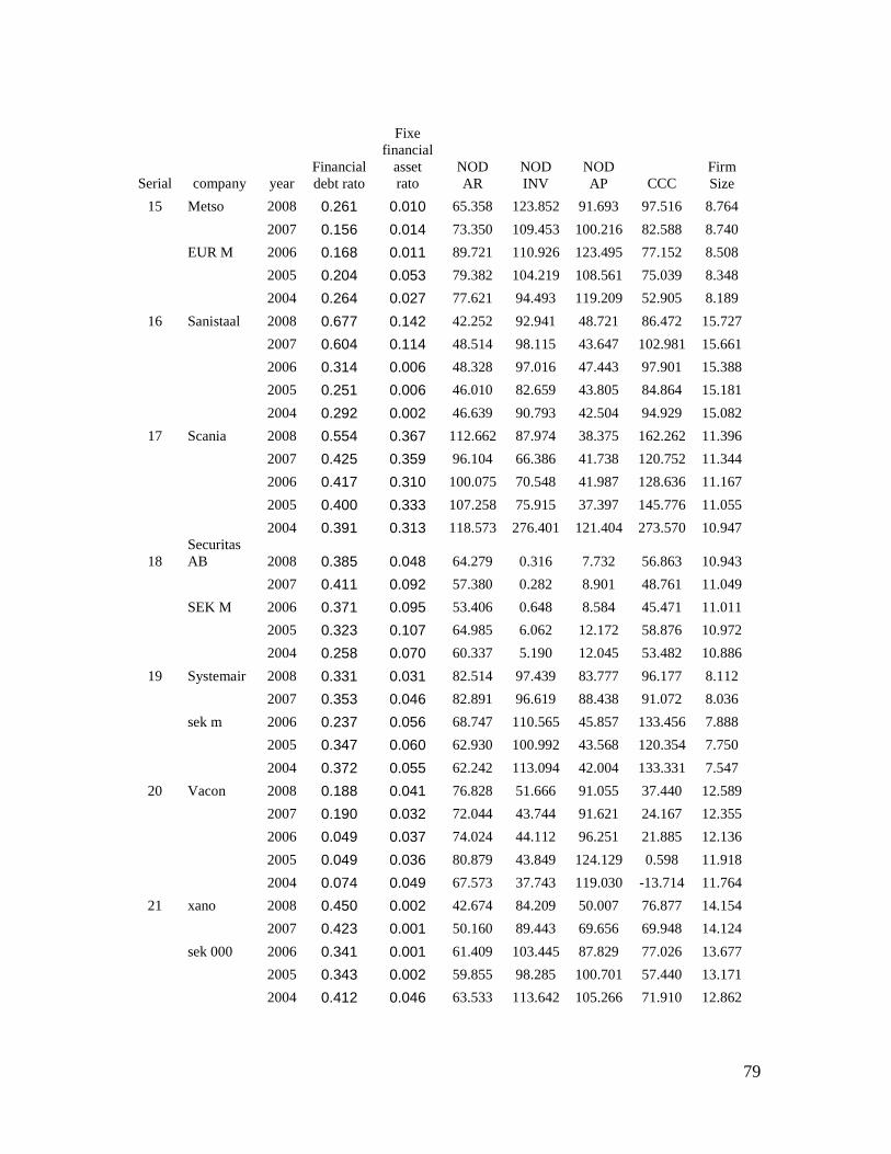
79

Serial company year Financial debt rato

Fixe financial

asset rato

NOD AR

NOD INV

NOD AP CCC

Firm Size

15 Metso 2008 0.261 0.010 65.358 123.852 91.693 97.516 8.764

2007 0.156 0.014 73.350 109.453 100.216 82.588 8.740

EUR M 2006 0.168 0.011 89.721 110.926 123.495 77.152 8.508

2005 0.204 0.053 79.382 104.219 108.561 75.039 8.348

2004 0.264 0.027 77.621 94.493 119.209 52.905 8.189

16 Sanistaal 2008 0.677 0.142 42.252 92.941 48.721 86.472 15.727

2007 0.604 0.114 48.514 98.115 43.647 102.981 15.661

2006 0.314 0.006 48.328 97.016 47.443 97.901 15.388

2005 0.251 0.006 46.010 82.659 43.805 84.864 15.181

2004 0.292 0.002 46.639 90.793 42.504 94.929 15.082

17 Scania 2008 0.554 0.367 112.662 87.974 38.375 162.262 11.396

2007 0.425 0.359 96.104 66.386 41.738 120.752 11.344

2006 0.417 0.310 100.075 70.548 41.987 128.636 11.167

2005 0.400 0.333 107.258 75.915 37.397 145.776 11.055

2004 0.391 0.313 118.573 276.401 121.404 273.570 10.947

18 Securitas AB 2008 0.385 0.048 64.279 0.316 7.732 56.863 10.943

2007 0.411 0.092 57.380 0.282 8.901 48.761 11.049

SEK M 2006 0.371 0.095 53.406 0.648 8.584 45.471 11.011

2005 0.323 0.107 64.985 6.062 12.172 58.876 10.972

2004 0.258 0.070 60.337 5.190 12.045 53.482 10.886

19 Systemair 2008 0.331 0.031 82.514 97.439 83.777 96.177 8.112

2007 0.353 0.046 82.891 96.619 88.438 91.072 8.036

sek m 2006 0.237 0.056 68.747 110.565 45.857 133.456 7.888

2005 0.347 0.060 62.930 100.992 43.568 120.354 7.750

2004 0.372 0.055 62.242 113.094 42.004 133.331 7.547

20 Vacon 2008 0.188 0.041 76.828 51.666 91.055 37.440 12.589

2007 0.190 0.032 72.044 43.744 91.621 24.167 12.355

2006 0.049 0.037 74.024 44.112 96.251 21.885 12.136

2005 0.049 0.036 80.879 43.849 124.129 0.598 11.918

2004 0.074 0.049 67.573 37.743 119.030 -13.714 11.764

21 xano 2008 0.450 0.002 42.674 84.209 50.007 76.877 14.154

2007 0.423 0.001 50.160 89.443 69.656 69.948 14.124

sek 000 2006 0.341 0.001 61.409 103.445 87.829 77.026 13.677

2005 0.343 0.002 59.855 98.285 100.701 57.440 13.171

2004 0.412 0.046 63.533 113.642 105.266 71.910 12.862

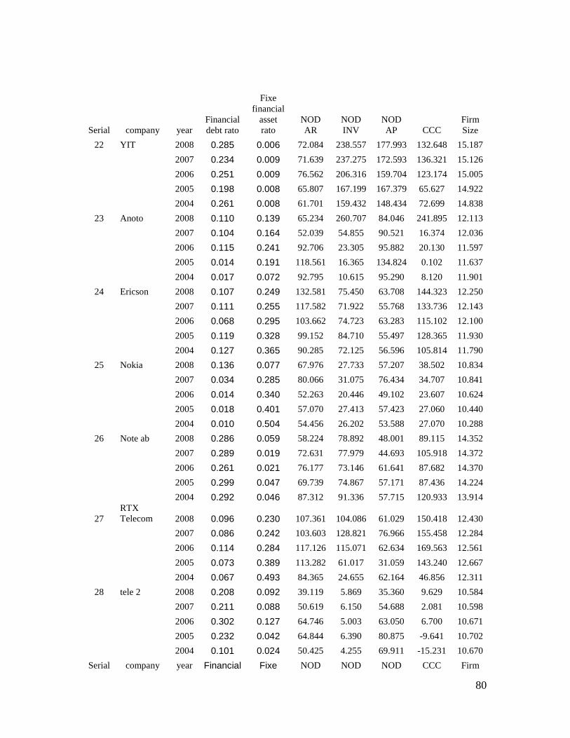
80

Serial company year Financial debt rato

Fixe financial

asset rato

NOD AR

NOD INV

NOD AP CCC

Firm Size

22 YIT 2008 0.285 0.006 72.084 238.557 177.993 132.648 15.187

2007 0.234 0.009 71.639 237.275 172.593 136.321 15.126

2006 0.251 0.009 76.562 206.316 159.704 123.174 15.005

2005 0.198 0.008 65.807 167.199 167.379 65.627 14.922

2004 0.261 0.008 61.701 159.432 148.434 72.699 14.838

23 Anoto 2008 0.110 0.139 65.234 260.707 84.046 241.895 12.113

2007 0.104 0.164 52.039 54.855 90.521 16.374 12.036

2006 0.115 0.241 92.706 23.305 95.882 20.130 11.597

2005 0.014 0.191 118.561 16.365 134.824 0.102 11.637

2004 0.017 0.072 92.795 10.615 95.290 8.120 11.901

24 Ericson 2008 0.107 0.249 132.581 75.450 63.708 144.323 12.250

2007 0.111 0.255 117.582 71.922 55.768 133.736 12.143

2006 0.068 0.295 103.662 74.723 63.283 115.102 12.100

2005 0.119 0.328 99.152 84.710 55.497 128.365 11.930

2004 0.127 0.365 90.285 72.125 56.596 105.814 11.790

25 Nokia 2008 0.136 0.077 67.976 27.733 57.207 38.502 10.834

2007 0.034 0.285 80.066 31.075 76.434 34.707 10.841

2006 0.014 0.340 52.263 20.446 49.102 23.607 10.624

2005 0.018 0.401 57.070 27.413 57.423 27.060 10.440

2004 0.010 0.504 54.456 26.202 53.588 27.070 10.288

26 Note ab 2008 0.286 0.059 58.224 78.892 48.001 89.115 14.352

2007 0.289 0.019 72.631 77.979 44.693 105.918 14.372

2006 0.261 0.021 76.177 73.146 61.641 87.682 14.370

2005 0.299 0.047 69.739 74.867 57.171 87.436 14.224

2004 0.292 0.046 87.312 91.336 57.715 120.933 13.914

27 RTX Telecom 2008 0.096 0.230 107.361 104.086 61.029 150.418 12.430

2007 0.086 0.242 103.603 128.821 76.966 155.458 12.284

2006 0.114 0.284 117.126 115.071 62.634 169.563 12.561

2005 0.073 0.389 113.282 61.017 31.059 143.240 12.667

2004 0.067 0.493 84.365 24.655 62.164 46.856 12.311

28 tele 2 2008 0.208 0.092 39.119 5.869 35.360 9.629 10.584

2007 0.211 0.088 50.619 6.150 54.688 2.081 10.598

2006 0.302 0.127 64.746 5.003 63.050 6.700 10.671

2005 0.232 0.042 64.844 6.390 80.875 -9.641 10.702

2004 0.101 0.024 50.425 4.255 69.911 -15.231 10.670

Serial company year Financial Fixe NOD NOD NOD CCC Firm

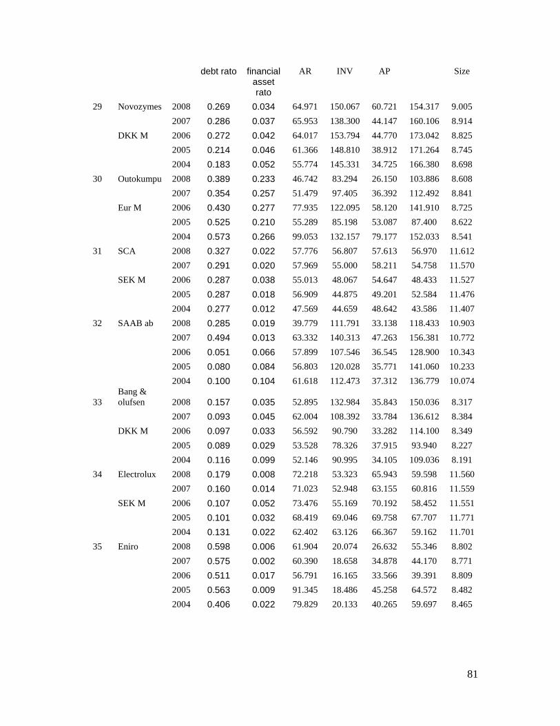
81

debt rato financial asset rato

AR INV AP Size

29 Novozymes 2008 0.269 0.034 64.971 150.067 60.721 154.317 9.005

2007 0.286 0.037 65.953 138.300 44.147 160.106 8.914

DKK M 2006 0.272 0.042 64.017 153.794 44.770 173.042 8.825

2005 0.214 0.046 61.366 148.810 38.912 171.264 8.745

2004 0.183 0.052 55.774 145.331 34.725 166.380 8.698

30 Outokumpu 2008 0.389 0.233 46.742 83.294 26.150 103.886 8.608

2007 0.354 0.257 51.479 97.405 36.392 112.492 8.841

Eur M 2006 0.430 0.277 77.935 122.095 58.120 141.910 8.725

2005 0.525 0.210 55.289 85.198 53.087 87.400 8.622

2004 0.573 0.266 99.053 132.157 79.177 152.033 8.541

31 SCA 2008 0.327 0.022 57.776 56.807 57.613 56.970 11.612

2007 0.291 0.020 57.969 55.000 58.211 54.758 11.570

SEK M 2006 0.287 0.038 55.013 48.067 54.647 48.433 11.527

2005 0.287 0.018 56.909 44.875 49.201 52.584 11.476

2004 0.277 0.012 47.569 44.659 48.642 43.586 11.407

32 SAAB ab 2008 0.285 0.019 39.779 111.791 33.138 118.433 10.903

2007 0.494 0.013 63.332 140.313 47.263 156.381 10.772

2006 0.051 0.066 57.899 107.546 36.545 128.900 10.343

2005 0.080 0.084 56.803 120.028 35.771 141.060 10.233

2004 0.100 0.104 61.618 112.473 37.312 136.779 10.074

33 Bang & olufsen 2008 0.157 0.035 52.895 132.984 35.843 150.036 8.317

2007 0.093 0.045 62.004 108.392 33.784 136.612 8.384

DKK M 2006 0.097 0.033 56.592 90.790 33.282 114.100 8.349

2005 0.089 0.029 53.528 78.326 37.915 93.940 8.227

2004 0.116 0.099 52.146 90.995 34.105 109.036 8.191

34 Electrolux 2008 0.179 0.008 72.218 53.323 65.943 59.598 11.560

2007 0.160 0.014 71.023 52.948 63.155 60.816 11.559

SEK M 2006 0.107 0.052 73.476 55.169 70.192 58.452 11.551

2005 0.101 0.032 68.419 69.046 69.758 67.707 11.771

2004 0.131 0.022 62.402 63.126 66.367 59.162 11.701

35 Eniro 2008 0.598 0.006 61.904 20.074 26.632 55.346 8.802

2007 0.575 0.002 60.390 18.658 34.878 44.170 8.771

2006 0.511 0.017 56.791 16.165 33.566 39.391 8.809

2005 0.563 0.009 91.345 18.486 45.258 64.572 8.482

2004 0.406 0.022 79.829 20.133 40.265 59.697 8.465

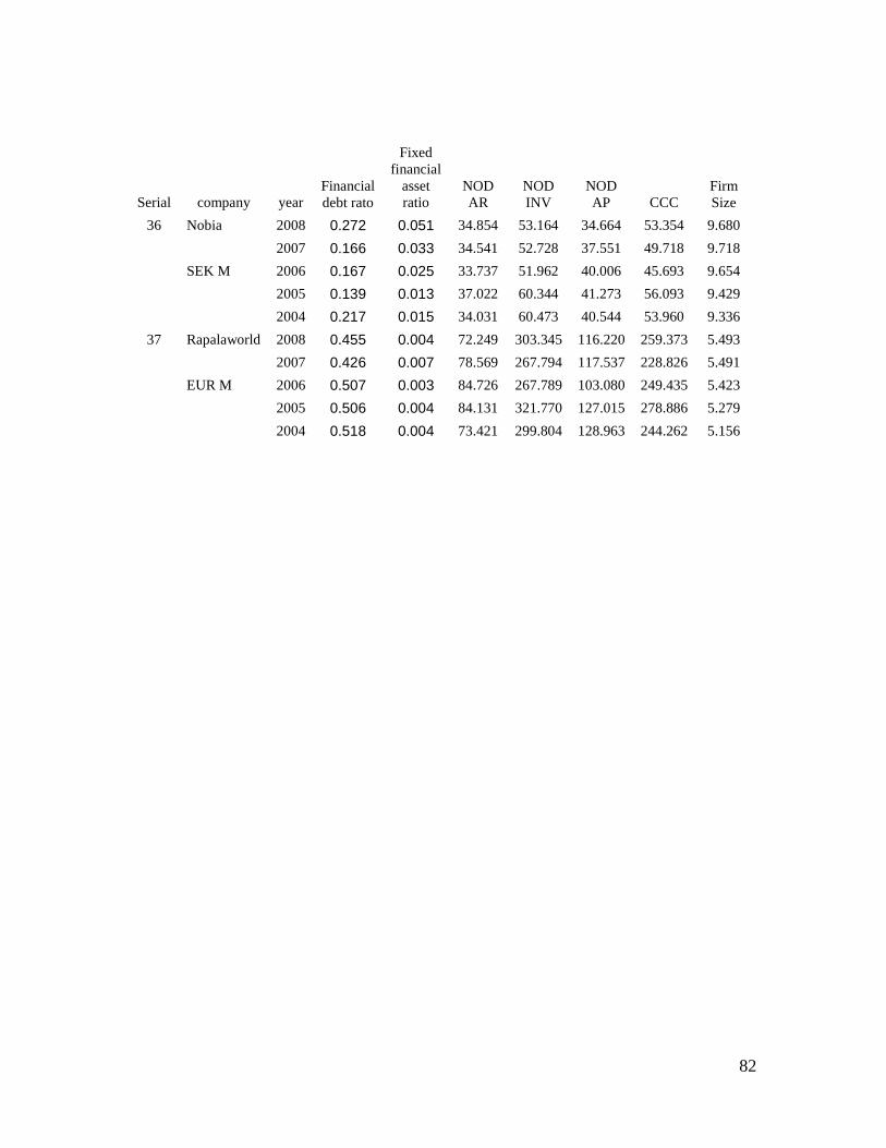
82

Serial company year Financial debt rato

Fixed financial

asset ratio

NOD AR

NOD INV

NOD AP CCC

Firm Size

36 Nobia 2008 0.272 0.051 34.854 53.164 34.664 53.354 9.680

2007 0.166 0.033 34.541 52.728 37.551 49.718 9.718

SEK M 2006 0.167 0.025 33.737 51.962 40.006 45.693 9.654

2005 0.139 0.013 37.022 60.344 41.273 56.093 9.429

2004 0.217 0.015 34.031 60.473 40.544 53.960 9.336

37 Rapalaworld 2008 0.455 0.004 72.249 303.345 116.220 259.373 5.493

2007 0.426 0.007 78.569 267.794 117.537 228.826 5.491

EUR M 2006 0.507 0.003 84.726 267.789 103.080 249.435 5.423

2005 0.506 0.004 84.131 321.770 127.015 278.886 5.279

2004 0.518 0.004 73.421 299.804 128.963 244.262 5.156

83

Umeå School of Business

Umeå University SE-901 87 Umeå, Sweden www.usbe.umu.se

84