Relationship between visual counts and call detection ratesof gray whales (Eschrichtius robustus) in LagunaSan Ignacio, Mexico

Diana Ponce, Aaron M. Thode,a) and Melania GuerraMarine Physical Laboratory, Scripps Institution of Oceanography, University of California San Diego,La Jolla, California 92093-0238

Jorge Urban R.Departamento de Biologıa Marina, Universidad Autonoma de Baja California Sur, Km 5.5 Carretera al Sur,Mezquitito, La Paz, B. C. S., 23080, Mexico

Steven SwartzLaguna San Ignacio Ecosystem Science Program, 14700 Springfield Road, Darnestown, Maryland 20874

(Received 25 March 2011; revised 30 January 2012; accepted 9 February 2012)

Daily acoustic calling rates of Eastern North Pacific (ENP) gray whales were measured on 6 days

during 1 mo of their 2008 breeding season in the sheltered coastal lagoon of Laguna San Ignacio in

Baja California, Mexico. Visual counts of whales determined that the numbers of single animals in

the lower lagoon more than tripled over the observation period. All call types showed production

peaks in the early morning and evening with minimum rates generally detected in the early

afternoon. For four of the five observation days, the daily number of “S1”-type calls increased

roughly as the square of the number of the animals in the lower lagoon during both daytime and

nighttime. This relationship persisted when raw call counts were adjusted for variations in back-

ground noise level, using a simple propagation law derived from empirical measurements. The one

observation day that did not fit the square-law relationship occurred during a week when the group

size in the lagoon increased rapidly. These results suggest that passive acoustic monitoring does not

measure gray whale group size directly but monitors the number of connections in the social

network, which rises as roughly M2/2 for a group size M.VC 2012 Acoustical Society of America. [http://dx.doi.org/10.1121/1.3689851]

PACS number(s): 43.30.Sf, 43.80.Ka, 43.80.Nd [WWA] Pages: 2700–2713

I. INTRODUCTION

A. Background on acoustic census efforts

Population estimates of marine mammals are currently

performed by visual surveys, which are restricted to daylight

hours and relatively calm weather conditions and can be

costly when conducted in the open ocean. By contrast, pas-

sive acoustic monitoring can be an effective, cost-efficient

technique for monitoring inaccessible habitats where visual

studies are difficult (Baptista and Gaunt, 1997). The use of

autonomous passive acoustic recorders to detect the seasonal

presence of marine mammals in various ocean basins has

become a popular technique, with a large accompanying lit-

erature (e.g., Stafford et al., 1998; Mellinger et al., 2004a;

Mellinger et al., 2004b; Moore et al., 2006; Mellinger et al.,2007a; Mellinger et al., 2007b; Munger et al., 2008). A natu-

ral question that arises is whether passive acoustic methods

can be used to estimate the relative or even absolute abun-

dance of marine mammal groups or population density—an

“acoustic census.”

Previous studies have used passive acoustic monitoring

to supplement traditional methods of estimating population

densities for terrestrial and aquatic organisms such as birds

(Dawson and Efford, 2009; Adi et al., 2010), elephants

(Payne et al., 2003; Thompson et al., 2010; Venter and

Hanekom, 2010), and marine mammals (McDonald and Fox,

1999; Douglas, 2000; Noad and Cato, 2000; Marques et al.,2009; Moretti et al., 2010; Kyhn et al., 2012). A practical

acoustic censusing method needs to overcome multiple chal-

lenges, including compensating for fluctuations in back-

ground noise levels, changing acoustic propagation

characteristics, and variations in animal behavior with

respect to age, sex, and multiple time scales. Perhaps the

greatest challenge required to establish the efficiency of any

acoustic censusing method on marine mammals is the diffi-

culty in determining an accurate independent estimate of

population density over appropriate spatial and temporal

time scales. Despite the increasing popularity of acoustic

censusing, few empirical studies exist that directly measure

the functional relationship between call detection rates and

population density due to the practical problem of independ-

ently verifying the acoustic population predictions. Most

previously published acoustic censuses of marine mammals

assume proportionality between sound detection rates and

population size (e.g., (Marques et al., 2009; Kyhn et al.,2012), although one study on beluga whales claimed to find

that the acoustic detection rate increased as the square of the

number of animals present (Simard et al., 2010).

a)Author to whom correspondence should be addressed. Electronic mail:

athode@ucsd.edu

2700 J. Acoust. Soc. Am. 131 (4), April 2012 0001-4966/2012/131(4)/2700/14/$30.00 VC 2012 Acoustical Society of America

Au

tho

r's

com

plim

enta

ry c

op

y

Here a simple acoustic census has been conducted at a

unique location that permits accurate visual surveys of a non-

captive marine mammal population. Between January and

March 2008, acoustic recordings of gray whales (Eschrichtiusrobustus) were collected in Laguna San Ignacio (LSI), Baja

California, Mexico, during the winter breeding season (Fig.

1). LSI is an enclosed coastal lagoon where gray whales

gather to breed and give birth during the northern hemisphere

winter. This study examines relationships between month-

long visual counts of gray whales and both raw and noise-

adjusted call detection rates for 6 days of acoustic recordings,

over daytime and nighttime, measured throughout February/

March in the lower region of the lagoon (Fig. 1). The instru-

ments have been deployed in the same location every year

since 2008, and some data collected in 2010 are used to esti-

mate acoustic propagation conditions in the area.

There are three reasons why LSI provides an excellent

laboratory for investigating the expected complex relation-

ships between sound production rates, group size, ambient

noise levels, and time of day. First, the lagoon’s restricted

geography, combined with the short dive times of the ani-

mals, enables frequent visual surveys to be conducted eco-

nomically and accurately. Second, breeding individuals

residing in the mouth of the lagoon (the “lower zone”

marked in Fig. 1) travel frequently from one location to

another, never loitering in one place for extended periods of

time. Thus the spatial distribution of whale acoustic activity

in the lagoon is expected to be relatively homogenous, such

that measurements of relative changes in acoustic activity on

a single hydrophone may represent relative changes in the

acoustic activity across the lower lagoon as a whole, which

in turn may be related to the total group size in the lower

zone. Finally, the ambient noise levels in the lagoon are rela-

tively steady over time; over the entire month, the hourly

noise levels varied by only 8–10 dB across the frequency

range of interest in this study. Therefore relatively simple

models can be used for adjusting sound detection rates for

changes in detection range arising from the ambient noise

fluctuations.

The rest of this introduction provides relevant back-

ground on the population trends and acoustic behavior of

Eastern North Pacific gray whales. Section II describes the

acoustic equipment, deployment location, visual survey pro-

cedures, and acoustic analysis methods, including methods

for adjusting call detection rates for changes in ambient

noise levels. Section III presents data manually analyzed

from 6 days of acoustic data collected over a 4-wk period off

Punta Piedra (Fig. 1), a prominent landmark in the lagoon.

These 4 wk captured the middle portion of the breeding sea-

son between February 10 and March 8, 2008, during which

the number of animals in the lower lagoon roughly tripled.

The section discusses sound detection rates for three gray

whale call types, the number of tourist boat transits, month-

long trends in raw call rates, changes in the ambient noise

background during the study, and measurements of the

acoustic propagation characteristics of the monitoring area.

Section IV discusses the diel patterns observed in two differ-

ent call types and interprets the long-term nonlinear relation-

ship observed between the visual counts and both the raw

and noise-adjusted daily detection counts for the most com-

mon call type (“S1”) detected.

B. Population trends of gray whales

Eastern North Pacific (ENP) gray whales seasonally

migrate from their summer feeding grounds in the Bering,

Chukchi, and (possibly) Beaufort Seas to coastal lagoons in

Baja California, Mexico. Historically, gray whale population

numbers have dramatically risen and fallen due to human ex-

ploitation and fluctuations in environmental conditions

affecting their food supply. Throughout the 19th century

commercial whalers harvested gray whales in major breed-

ing lagoons and bays of Baja California, killing an estimated

7,000–8,000 gray whales (Henderson 1984). Continued

hunting into the 20th century reduced the population to crit-

ically low numbers, and the gray whale finally received

international protection from commercial whaling by the

International Whaling Commission in 1946. By the 1960s,

the gray whale population was estimated to be 15,000 whales

(Rice and Wolman, 1971), and three decades later, in 1998,

the population had recovered to an estimated historical level

of around 21,000 whales. Following a range-wide mortality

event from 1998 to 2000, a 2002 census indicated the

population had been reduced to 16,000 whales; however, as

of 2006–2007, the gray whale population was estimated

to have recovered to approximately 19,000 whales

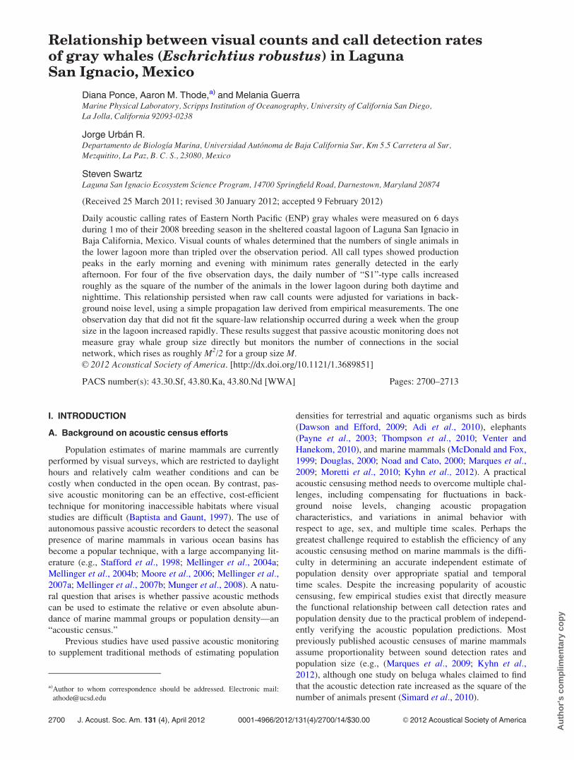
FIG. 1. (Color online) Map of Laguna San Ignacio (LSI), including 2008

and 2010 deployment location of acoustic hydrophone (solid triangle),

which is similar to the cabled hydrophone location used by (Dahlheim,

1987). Visual surveys of gray whale population studies are subdivided into

three zones indicated by dashed lines. An additional site in 2010 (filled

circle) was deployed 1.5 km away to evaluate propagation conditions.

J. Acoust. Soc. Am., Vol. 131, No. 4, April 2012 Ponce et al.: Gray whale acoustic census 2701

Au

tho

r's

com

plim

enta

ry c

op

y

(Laake et al., 2009). Only a small fraction of the total gray

whale population winters at LSI. This lagoon remains pro-

tected from commercial whaling and most industrial devel-

opment as a federal marine protected area and whale refuge,

and it lies within Mexico’s Vizcaino Biosphere Reserve. As

a protected wildlife reserve, the lagoon and its gray whales

attracted the development of eco-tourism camps along its

southern shore. There remains considerable scientific and

socio-economical interest in monitoring gray whale numbers

in the lagoon each winter as an indicator of the general status

of the ENP gray whale population.

The lagoon’s relatively small size, high density of adult

whales and calves, and cooperative efforts with the local

eco-tourism industry has attracted research attention for dec-

ades. The lagoon has also attracted researchers due to its rel-

atively isolated location, low levels of commercial

development, and restrictions on the levels of tourist activity

permitted in the lagoon. These factors provide a relatively

undisturbed environment to study whale behavior, and the

lagoon thus boasts a long history of visual and acoustic stud-

ies of gray whales dating back to the mid-1970s. After an

initial period of annual surveys during the period 1977–1982

(Jones and Swartz, 1984), regular visual censuses of the

whales in the lagoon were conducted only between 1996 and

2000. Regular systematic visual surveys were resumed in

2006, by the Laguna San Ignacio Ecosystem Science Pro-

gram (LSIESP; www.lsiecosystem.org; last accessed Jan 30,

2012). The LSIESP team also documents individual whales

using photographic identification (photo-ID) methods.

C. Gray whale acoustic behavior

The acoustic repertoire of gray whales has been primar-

ily studied in the breeding-calving lagoons of Baja Califor-

nia (Dahlheim, 1987; Wisdom 2000; Ollervides, 2001), with

less extensive efforts along the North American Pacific coast

(Cummings et al., 1968; Crane and Lashkari, 1996), and arc-

tic waters (Moore et al., 2006; Stafford et al., 2007). In this

paper, we restrict our review to sounds collected in LSI,

where studies of gray whale acoustics have a relatively long

history.

During winter seasons between 1981 and 1984, Dahl-

heim et al. (Dahlheim et al., 1984; Dahlheim, 1987) con-

ducted the first gray whale recordings in LSI by deploying

an omni-directional hydrophone near Punta Piedra (Fig. 1).

Her findings, distilled from a cumulative 565 hours of under-

water recordings, discerned six types of calls, of which three

are discussed in this paper. Over a decade later, Wisdom etal. (Wisdom, 2000) collected gray whale recordings from

hydrophones deployed from a small 4-m boat, locally

referred to as a panga.

Both studies have revealed that LSI gray whales pro-

duce sounds ranging from rapid, rhythmic pulses to FM sig-

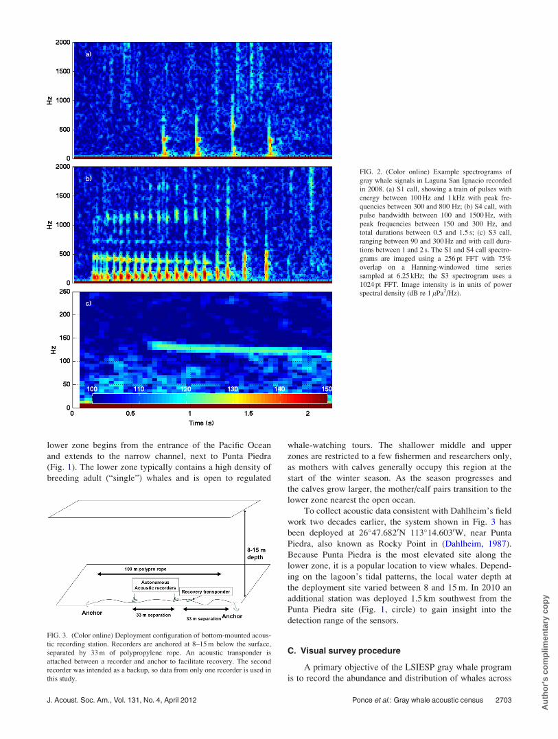
nals. Gray whales produce an assorted collection of pulsed

calls, with the so-called “S1” pulsed calls being predominant

[Fig. 2(a)]. Individual pulses range in frequency between

100 and 1600 Hz and are grouped in sets of 3–18 pulses per

call. Peak frequencies range between 300 and 800 Hz, and

call durations average 1.8 s (Dahlheim et al., 1984). A sec-

ond type of pulsed call, the “S4” [Fig. 2(b)], is characterized

by clustered pulses with intervals much smaller than the S1

call, frequency content between 100 and 800 Hz, with peak

frequencies between 150 and 300 Hz, and durations averag-

ing between 0.5 and 1.5 s. A third call type, “S3”, is an FM

signal typically averaging 1.5 s per call [Fig. 2(c)]. This call

is characterized by relatively low frequencies, ranging

between 100 and 300 Hz. Wisdom (2000) reported the S3 as

being the least common call type, comprising only 3% of her

recorded calls. She also defined two additional call types: 1 b

and the “rumble.” Sound type 1 b is a pulsed signal, whereas

“rumble” is a sound that Wisdom recorded in the presence of

active calves.

Most researchers have concluded that gray whale sounds

are not sonar signals but fill a social function (Wisdom,

2000). Previous studies suggest that these sounds might be

used for communication purposes such as contact calling

(Fish et al., 1974; Norris et al., 1977), species recognition

(Dahlheim et al., 1984), and providing behavioral context

(Crane and Lashkari, 1996).

Three of the six call types identified by Dahlheim (S1,

S3, S4) are used in this study, because these three calls were

commonly found in the 2008 acoustic data set and were also

easy to identify and distinguish from each other. Other call

types, although present, were relatively uncommon, making

conclusive identification difficult, based only on the descrip-

tions and examples in Dahlheim’s and Wisdom’s theses.

II. MATERIALS AND METHODS

A. Acoustic recording equipment

Acoustic data were collected by a cylindrical, bottom-

mounted recorder that contained a Persistor CF2 microproc-

essor, 60 GB hard drive, 4 GB flash memory chip, D-cell

batteries, and a HTI-96-MIN hydrophone with sensitivity of

�171.4 dB re 1 V/lPa. These electronics were packed inside

a 12 cm diameter by 75 cm long acrylic pressure housing and

then deployed from a small boat. In 2008, acoustic data were

sampled at 6.125 kHz, and after recording for 67 h to flash

memory, the device halted audio sampling for 1.75 h to

transfer the data to hard disk. That year, the instrument

recorded for 29 days before the batteries discharged. Deploy-

ments were also conducted in 2010, with a sampling rate of

12.5 kHz.

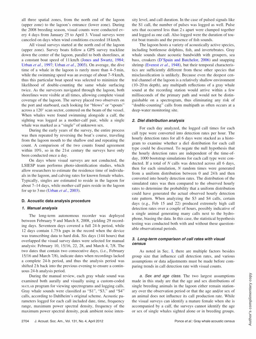
As shown in Fig. 3, during both years, two recorders

were strapped to a 100 m polypropylene rope, which was

deployed horizontally on the lagoon floor, with 10 kg

anchors attached on both ends. The second recorder was

intended as a backup system, so data from only one recorder

are used in this study. The system was recovered using grap-

pling hooks to avoid the use of surface buoys that could

entangle whales. A HOBO weather station was also

deployed onshore Punta Piedra to help determine relation-

ships between local wind speed and ambient noise levels.

B. Field site

Visual surveys were conducted by LSIESP, and divided

the lagoon into three zones: upper, middle, and lower. The

2702 J. Acoust. Soc. Am., Vol. 131, No. 4, April 2012 Ponce et al.: Gray whale acoustic census

Au

tho

r's

com

plim

enta

ry c

op

y

lower zone begins from the entrance of the Pacific Ocean

and extends to the narrow channel, next to Punta Piedra

(Fig. 1). The lower zone typically contains a high density of

breeding adult (“single”) whales and is open to regulated

whale-watching tours. The shallower middle and upper

zones are restricted to a few fishermen and researchers only,

as mothers with calves generally occupy this region at the

start of the winter season. As the season progresses and

the calves grow larger, the mother/calf pairs transition to the

lower zone nearest the open ocean.

To collect acoustic data consistent with Dahlheim’s field

work two decades earlier, the system shown in Fig. 3 has

been deployed at 26�47.6820N 113�14.6030W, near Punta

Piedra, also known as Rocky Point in (Dahlheim, 1987).

Because Punta Piedra is the most elevated site along the

lower zone, it is a popular location to view whales. Depend-

ing on the lagoon’s tidal patterns, the local water depth at

the deployment site varied between 8 and 15 m. In 2010 an

additional station was deployed 1.5 km southwest from the

Punta Piedra site (Fig. 1, circle) to gain insight into the

detection range of the sensors.

C. Visual survey procedure

A primary objective of the LSIESP gray whale program

is to record the abundance and distribution of whales across

FIG. 2. (Color online) Example spectrograms of

gray whale signals in Laguna San Ignacio recorded

in 2008. (a) S1 call, showing a train of pulses with

energy between 100 Hz and 1 kHz with peak fre-

quencies between 300 and 800 Hz; (b) S4 call, with

pulse bandwidth between 100 and 1500 Hz, with

peak frequencies between 150 and 300 Hz, and

total durations between 0.5 and 1.5 s; (c) S3 call,

ranging between 90 and 300 Hz and with call dura-

tions between 1 and 2 s. The S1 and S4 call spectro-

grams are imaged using a 256 pt FFT with 75%

overlap on a Hanning-windowed time series

sampled at 6.25 kHz; the S3 spectrogram uses a

1024 pt FFT. Image intensity is in units of power

spectral density (dB re 1 lPa2/Hz).

FIG. 3. (Color online) Deployment configuration of bottom-mounted acous-

tic recording station. Recorders are anchored at 8–15 m below the surface,

separated by 33 m of polypropylene rope. An acoustic transponder is

attached between a recorder and anchor to facilitate recovery. The second

recorder was intended as a backup, so data from only one recorder is used in

this study.

J. Acoust. Soc. Am., Vol. 131, No. 4, April 2012 Ponce et al.: Gray whale acoustic census 2703

Au

tho

r's

com

plim

enta

ry c

op

y

all three spatial zones, from the north end of the lagoon

(upper zone) to the lagoon’s entrance (lower zone). During

the 2008 breeding season, visual counts were conducted ev-

ery 4 days from January 25 to April 3. Visual surveys were

canceled on days when wind conditions exceeded 18 km/h.

All visual surveys started at the north end of the lagoon

(upper zone). Survey boats follow a GPS survey trackline

down the center of the lagoon, parallel to both shorelines, at

a constant boat speed of 11 km/h (Jones and Swartz, 1984;

Urban et al., 1997; Urban et al., 2003). On average, the dive

time of a whale in the lagoon is rarely more than 4–5 min,

while the swimming speed was an average of about 7–9 km/h,

thus this particular boat speed was selected to minimize the

likelihood of double-counting the same whale surfacing

twice. As the surveyors navigated through the lagoon, both

shorelines were visible at all times, allowing complete visual

coverage of the lagoon. The survey placed two observers on

the port and starboard, each looking for “blows” or “spouts”

across a 120� scan sector, centered on the beam of the vessel.

When whales were found swimming alongside a calf, the

sighting was logged as a mother-calf pair, while a single

whale was marked as a “single” of unknown sex.

During the early years of the survey, the entire process

was then repeated by reversing the boat’s course, traveling

from the lagoon mouth to the shallow end and repeating the

count. A comparison of the two counts found agreement

within 10%, so in the 21st century the surveys have only

been conducted once a day.

On days where visual surveys are not conducted, the

LSIESP team performs photo-identification studies, which

allow researchers to estimate the residence time of individu-

als in the lagoon, and calving rates for known female whales.

Typically, singles are estimated to reside in the lagoon for

about 7–14 days, while mother-calf pairs reside in the lagoon

for up to 3 mo (Urban et al., 2003).

D. Acoustic data analysis procedure

1. Manual analysis

The long-term autonomous recorder was deployed

between February 9 and March 8, 2008, yielding 29 record-

ing days. Seventeen days covered a full 24-h period, while

12 days contain 1.75 h gaps in the record when the device

was transcribing data to hard disk. Six days (144 hours) that

overlapped the visual survey dates were selected for manual

analysis: February 10, 15/16, 22, 28, and March 4, 7/8. The

two dates that contain two consecutive days, (i.e., February

15/16 and March 7/8), indicate dates when recordings lacked

a complete 24-h period, and thus the analysis period was

shifted 2 h back into the previous evening to ensure a contin-

uous 24-h analysis period.

During the manual review, each gray whale sound was

examined both aurally and visually using a custom-coded

MATLAB program for viewing spectrograms and logging calls.

Gray whale sounds were classified as “S1”, “S3,” and “S4”

calls, according to Dahlheim’s original scheme. Acoustic pa-

rameters logged for each call included date, time, frequency

range, maximum power spectral density, frequency of the

maximum power spectral density, peak ambient noise inten-

sity level, and call duration. In the case of pulsed signals like

the S1 call, the number of pulses was logged as well. Pulse

sets that occurred less than 2 s apart were clumped together

and logged as one call. Also logged were the duration of tou-

rist boat transits and the presence of fish sounds.

The lagoon hosts a variety of acoustically active species,

including bottlenose dolphins, fish, and invertebrates. Gray

whale sounds share acoustic bandwidth with groupers, sea

bass, croakers (D’Spain and Batchelor, 2006) and snapping

shrimp (Everest et al., 1948), but their temporal characteris-

tics are sufficiently different from these other species that

misclassification is unlikely. Because even the deepest cen-

tral channel of the lagoon is a relatively shallow environment

(10–20 m depth), any multipath reflections of a gray whale

sound at the recording station would arrive within a few

milliseconds of the primary path and would not be distin-

guishable on a spectrogram, thus eliminating any risk of

“double-counting” calls from multipath as often occurs at a

deep-water monitoring site.

2. Diel distribution analysis

For each day analyzed, the logged call times for each

call type were converted into detection rates per hour. The

hourly detection rates for all 6 days were stacked as a histo-

gram to examine whether a diel distribution for each call

type could be discerned. To negate the null hypothesis that

the hourly detection rates are independent of the time-of-

day, 1000 bootstrap simulations for each call type were con-

ducted. If a total of N calls was detected across all 6 days,

then for each simulation, N random times were generated

from a uniform distribution between 0 and 24 h and then

converted into hourly detection rates. The distribution of the

simulated rates was then compared to the observed hourly

rates to determine the probability that a uniform distribution

could have generated the actual observed hourly detection

rate pattern. When analyzing the S3 and S4 calls, certain

days (e.g., Feb 15 and 22) produced extremely high call

detection rates over a couple of hours, possibly indicative of

a single animal generating many calls next to the hydro-

phone, biasing the data. In this case, the statistical hypothesis

testing was conducted both with and without these question-

able observational periods.

3. Long-term comparison of call rates with visualcensus

As noted in Sec. I, there are multiple factors besides

group size that influence call detection rates, and various

assumptions or data adjustments must be made before com-

paring trends in call detection rate with visual counts.

a. Sex and age class. The two largest assumptions

made in this study are that the age and sex distributions of

single breeding animals in the lagoon either remain station-

ary over the observation period or that the age and/or sex of

an animal does not influence its call production rate. While

the visual surveys can identify a mature female when she is

accompanied by a calf, the surveys cannot identify the age

or sex of single whales sighted alone or in breeding groups.

2704 J. Acoust. Soc. Am., Vol. 131, No. 4, April 2012 Ponce et al.: Gray whale acoustic census

Au

tho

r's

com

plim

enta

ry c

op

y

As the average residence time of breeding individuals is on

the order of days (Urban et al., 2003), the group of individu-

als recorded at the end of the study is likely not the same

group of individuals at the start of the study. Thus we must

assume that the sex and age ratios of the single animal

groups in LSI do not systematically change over the course

of the observational study or that any such change is irrele-

vant to the acoustic behavior of the group.

b. Behavioral state and time-of-day. The types and

rate of acoustic vocalizations made by animals can vary with

its behavioral state, which in turn depends on a variety of

factors, including time of day and mean group size. The

presence of a diel pattern in call detection rate is an example

of the former factor. To compensate for these effects, the

total number of each type of call detected over each contigu-

ous 24-h period defined in Sec. II D 1 is computed and is

defined here as the “raw” daily call count. By summing call

detections over a full 24-h period to generate a raw count,

we attempt to remove diel effects, as well as effectively av-

erage over the acoustic behavioral states a gray whale dis-

plays over the time scale of a day. Changes in individual

behavior that arise from changes in group size (or “density-

dependent effects”) over longer time scales will not be com-

pensated by using daily counts, with consequences that will

be seen in Sec. III.

c. Anthropogenic effects. While LSI remains a rela-

tively undisturbed environment, it does host a vibrant whale-

watching tourism industry that uses small boats to carry tou-

rists for encounters with whales. If the number of daily boat

tours was to change substantially over the course of the

month-long observation period, then one cannot discount the

potential effects of this boat activity on either the sound pro-

duction rates of the animals or the ability of the sensor to

detect gray whale sounds.

Fortunately, no tourism (or any human activity) takes

place on the lagoon between 1 h before sunset and 1 h after

sunrise. Thus one can compute not only a daily call count

but also a “daytime” call count (computed between 08:00

and 18:00) and a “nighttime” call count (computed from

18:00 to 08:00 the following day), which also represent time

periods with and without boat noise, respectively. If the

long-term trends of the daytime and nighttime counts are

similar, then the impact of tourist activity on long-term call

counts can be discounted (unless the potential diel effects

and tourist effects cancel each other out perfectly; an

unlikely situation, given that both effects would be expected

to decrease call detection rates during the daytime; Sec. IV A

discusses how diel patterns observed for other marine mam-

mals tend to show lower detection rates during the day).

d. Background noise levels. A crucial factor affecting

call detection rates is the level of background noise present

during a particular observation time. If the background noise

levels increase, then hourly call detection rates would be

expected to fall if all other factors remain constant. As dis-

cussed in Sec. I, the variation in ambient noise levels in LSI

is relatively mild compared to open-ocean acoustic condi-

tions; however, it will be shown that fluctuations of “only”

3 dB in background noise levels can still translate into a fac-

tor of two change in call detection rates, depending on the

propagation environment. Therefore an essential step for anyacoustic census study, including this one, is estimating the

impact of background noise variations on results derived

from acoustic data.

In this study “raw” call counts are distinguished from

“noise-adjusted” call counts. Raw call counts are counts

obtained directly from the data, and the noise-adjusted

counts are raw counts adjusted for variations in background

noise levels over hourly time scales. The next subsection

introduces the noise-adjustment model in detail.

4. Adjusting raw call rates for differences inbackground noise levels

The noise-adjustment model applies a simplified version

of the sonar equation to translate changes in background

noise level into an adjusted hourly detection rate. The cost of

simplicity is the necessity of making several significant

assumptions about the distribution of animals, their acoustic

behavior, and the propagation environment.

The first assumption in the model states that a relative

change in the number of vocalizing animals, measured

within the small area being monitored, matches the relative

change of all vocalizing animals in the lower zone of the

lagoon. The key assumption here is not detection range but

whether animals are evenly distributed throughout the lower

zone to ensure a subsample of a small region is considered

representative of the whole. Observations of the LSIESP

photo ID team, along with VHF and satellite tagging data,

indicate that single animals do frequently traverse across and

exit from the lower lagoon area, never remaining in one

place for long (Mate et al., 2003; Urban et al., 2003), sug-

gesting that this assumption is reasonable.

Second, the model assumes the lagoon is sufficiently

shallow for there to be a proportional relationship between

the volume of water accessible to the sensor and the square

of the detection range (area of coverage), instead of the cube

of the detection range (as would be the case in deep waters

of the open ocean). Under this assumption, the detection

range of the sensor must be less than the width of the lagoon

at Punta Piedra (Fig. 1). In a situation where the detection

range of a single sensor is larger than this geographic spatial

scale, the detection area would become a highly non-linear

function of detection range, due to the presence of the oppo-

site shoreline and shadowing features related to dramatic ba-

thymetry profiles present in the lagoon. The fact that the

sensor is positioned near a peninsula and is effectively

blocked from detecting sounds from all azimuths does not

violate this assumption, as a circular wedge increases as the

square of detection range. Section III D discusses experi-

mental measurements and numerical simulations of the

detection range around the sensor to support this assumption.

Third, the model assumes that the source level distribu-

tion of calls and potential diel acoustic behaviors remain

invariant with changes in background noise level. There is

evidence that baleen whales increase their source levels to

J. Acoust. Soc. Am., Vol. 131, No. 4, April 2012 Ponce et al.: Gray whale acoustic census 2705

Au

tho

r's

com

plim

enta

ry c

op

y

compensate for increases in background noise levels (e.g.,

Parks et al., 2007), so this assumption may be invalid. How-

ever, if gray whales do adjust their source levels in response

to changes in ambient noise level, then the appropriate call

detection counts would be expected to lie somewhere

between the raw call counts (which effectively assume that

whales compensate perfectly for ambient noise level

changes) and the noise-adjusted counts derived here (which

assume that whales do not compensate for ambient noise

level changes). Thus in the Secs. III and IV, both the raw

and noise-adjusted counts are presented, and the relative im-

portance of assuming a constant source level distribution can

be judged by comparing the relative differences in the raw

and noise-adjusted counts.

The fourth assumption is that all calls above a certain

signal-to-noise ratio (SNR) threshold are assumed detected

by a manual analyst. The actual value of the SNR threshold

where this fall-off occurs is not relevant to the derivation.

Finally, a very simple propagation model is assumed,

where the square-pressure of a discrete acoustic signal from

a compact source is assumed to fall off with horizontal range

r as r�a. Another way of stating this assumption is that the

dB transmission loss of an acoustic field falls off as

10alog10(r). Note that this assumption, like the second

assumption, requires that the effective detection range of the

sensor be significantly smaller than the width of the lagoon

at Punta Piedra. Section III D discusses simulations and field

measurements of the sound propagation factor a.

From these assumptions, the following expression can

be derived for adjusting a daily raw call count for differences

in ambient noise levels:

Cj;adj ¼X24

i¼1

Cij;rawNij

Nref

� �2=a

: (1)

Here Cij,raw is the number of calls manually detected on hour

i of date j, and Nij is the noise level measured over that same

hour, integrated over the bandwidth of the call type in ques-

tion. Note that N is expressed in linear units and not decibel

units. To obtain daytime and nighttime adjusted call counts,

the summation in Eq. (1) is conducted only over the appro-

priate hours of the day discussed in Sec. II D 3. The quantity

in parentheses, raised to the power of 2/a, is defined here as

the “call multiplier.”

Nij is computed by first integrating a set of instantaneous

power spectral densities (PSD) between 350 and 750 Hz,

using a 1024-pt FFT, overlapped 50%. Every 2 min, the min-

imum integrated PSD value encountered is retained, provid-

ing 30 values an hour. These values are averaged in the

linear (not dB) domain to obtain Nij. Consequently, the aver-

age of a set of minimum background noise levels is captured,

instead of a simple average of all PSD estimates, to exclude

numerous impulsive events like snapping shrimp from the

noise calculation, under the reasoning that moderate amounts

of impulsive noise do not reduce the ability to detect an S1

call. Nref is a particular reference noise level; here

Nref ¼ 104 dB re 1 lPa (rms), integrated between 350 and

750 Hz, is used as a representative value for non-pulsive

ambient noise conditions in the lagoon. Equation (1) can

also be derived from the density estimation formalism of

Eqs. (3), (5), and (6) in (Marques et al., 2009), assuming a

Heaviside “step” function for g(y) with detection range wdetermined by SNR.

A glance at Eq. (1) shows that call counts on relatively

noisy days are adjusted upward under the assumption that

more calls would have been detected at the (quieter) refer-

ence noise level. For a equal to 2 (spherical spreading), the

adjusted call counts become proportional to background

noise values, such that a 3 dB increase (doubling) in noise

level will result in a doubling of the adjusted call count, rela-

tive to the raw call count, over that hourly measurement.

The larger the value of a, (i.e., the worse the propagation

conditions), the less sensitive the call-adjustment formula

becomes to fluctuations in ambient noise.

To permit direct comparison, acoustic and visual counts

are occasionally presented in relative terms with respect to

the first visual census day. For example, the raw and noise-

adjusted daily call counts are divided by the raw and noise-

adjusted call counts from the first day. Similarly, the visual

census counts are divided by the visual census count on the

first day, permitting the normalized acoustic and visual

measurements to be plotted together. As the acoustic data

were collected on the boundary between the lower and mid-

dle zones, visual data from both the lower zone and the com-

bined middle and lower zones will be presented.

III. RESULTS

A. Diel pattern in call rates

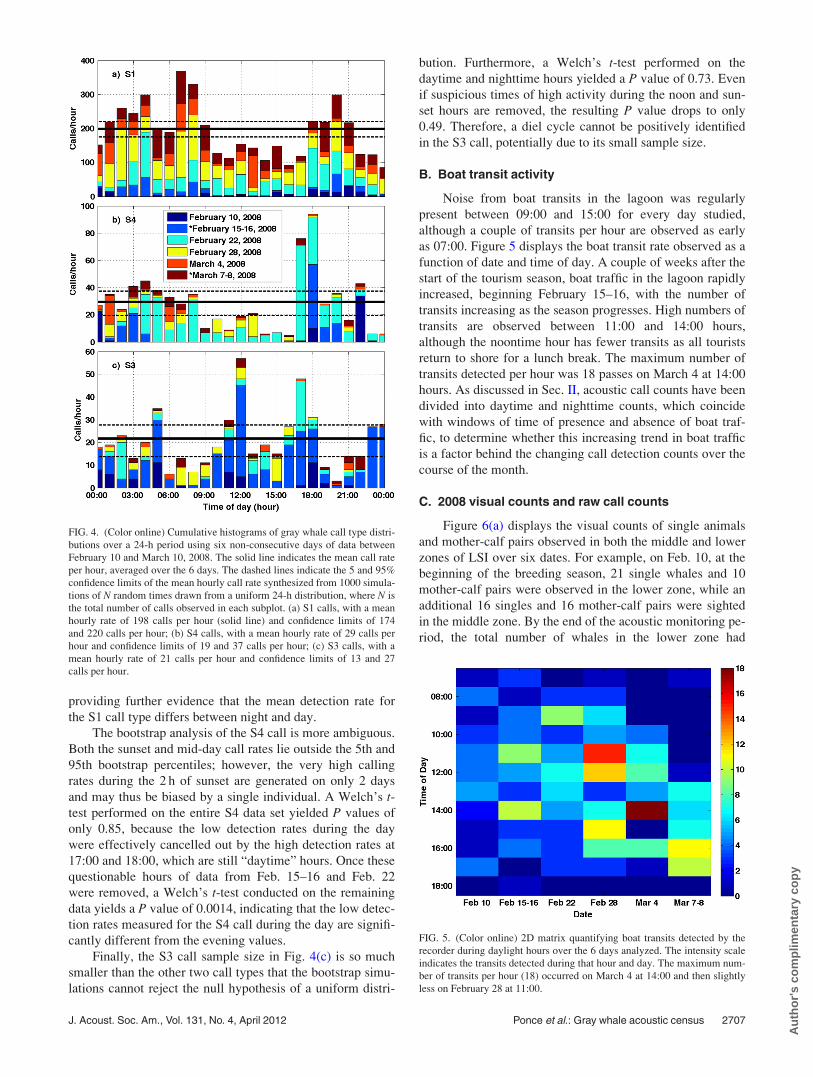
Figure 4 shows the hourly raw call distributions for the

S1, S3, and S4 sounds detected near Punta Piedra, stacked

over 6 days. The total raw call counts across all days were

4757 S1 calls, 705 S4 calls, and 520 S3 calls. The horizontal

solid lines in Fig. 4 display the average raw call rate com-

puted over the entire 6-day period, while the dashed lines

indicate the 5th and 95th percentiles of the mean hourly call

rate derived from the bootstrap simulations discussed in Sec.

II D 2. Hourly call rates that lie between the dashed lines

cannot reject the null hypothesis that they were generated

from a uniform (time-independent) calling distribution.

The histograms suggest that S1 and S4 calling activity

levels are greatest around dawn and twilight hours. By con-

trast, by mid-morning and mid-afternoon, these call types

are detected at rates at least 40% below the 24-h averaged

calling rate. For example, the S1 call [Fig. 4(a)] shows an

obvious decrease in calling activity between 10:00 and 15:00

hours in comparison to the rest of the day. For the S1 call,

the high rates at dusk and dawn and the low rates during

mid-morning and mid-afternoon lie outside the 5th and 95th

percentile lines for the uniform distribution, indicating that

the null hypothesis of a uniform (non-diel) distribution can

be rejected. In addition to the bootstrap simulations, two-

sample t-test and Welch’s approximate t-test were also con-

ducted on the S1 data comparing daytime detection rates

(between 08:00 and 18:00) with nighttime rates. The two-

sample t-test and Welch’s test yielded P values of

1.85� 10�4 and 2.47� 10�4, respectively, for the S1 data,

2706 J. Acoust. Soc. Am., Vol. 131, No. 4, April 2012 Ponce et al.: Gray whale acoustic census

Au

tho

r's

com

plim

enta

ry c

op

y

providing further evidence that the mean detection rate for

the S1 call type differs between night and day.

The bootstrap analysis of the S4 call is more ambiguous.

Both the sunset and mid-day call rates lie outside the 5th and

95th bootstrap percentiles; however, the very high calling

rates during the 2 h of sunset are generated on only 2 days

and may thus be biased by a single individual. A Welch’s t-test performed on the entire S4 data set yielded P values of

only 0.85, because the low detection rates during the day

were effectively cancelled out by the high detection rates at

17:00 and 18:00, which are still “daytime” hours. Once these

questionable hours of data from Feb. 15–16 and Feb. 22

were removed, a Welch’s t-test conducted on the remaining

data yields a P value of 0.0014, indicating that the low detec-

tion rates measured for the S4 call during the day are signifi-

cantly different from the evening values.

Finally, the S3 call sample size in Fig. 4(c) is so much

smaller than the other two call types that the bootstrap simu-

lations cannot reject the null hypothesis of a uniform distri-

bution. Furthermore, a Welch’s t-test performed on the

daytime and nighttime hours yielded a P value of 0.73. Even

if suspicious times of high activity during the noon and sun-

set hours are removed, the resulting P value drops to only

0.49. Therefore, a diel cycle cannot be positively identified

in the S3 call, potentially due to its small sample size.

B. Boat transit activity

Noise from boat transits in the lagoon was regularly

present between 09:00 and 15:00 for every day studied,

although a couple of transits per hour are observed as early

as 07:00. Figure 5 displays the boat transit rate observed as a

function of date and time of day. A couple of weeks after the

start of the tourism season, boat traffic in the lagoon rapidly

increased, beginning February 15–16, with the number of

transits increasing as the season progresses. High numbers of

transits are observed between 11:00 and 14:00 hours,

although the noontime hour has fewer transits as all tourists

return to shore for a lunch break. The maximum number of

transits detected per hour was 18 passes on March 4 at 14:00

hours. As discussed in Sec. II, acoustic call counts have been

divided into daytime and nighttime counts, which coincide

with windows of time of presence and absence of boat traf-

fic, to determine whether this increasing trend in boat traffic

is a factor behind the changing call detection counts over the

course of the month.

C. 2008 visual counts and raw call counts

Figure 6(a) displays the visual counts of single animals

and mother-calf pairs observed in both the middle and lower

zones of LSI over six dates. For example, on Feb. 10, at the

beginning of the breeding season, 21 single whales and 10

mother-calf pairs were observed in the lower zone, while an

additional 16 singles and 16 mother-calf pairs were sighted

in the middle zone. By the end of the acoustic monitoring pe-

riod, the total number of whales in the lower zone had

FIG. 4. (Color online) Cumulative histograms of gray whale call type distri-

butions over a 24-h period using six non-consecutive days of data between

February 10 and March 10, 2008. The solid line indicates the mean call rate

per hour, averaged over the 6 days. The dashed lines indicate the 5 and 95%

confidence limits of the mean hourly call rate synthesized from 1000 simula-

tions of N random times drawn from a uniform 24-h distribution, where N is

the total number of calls observed in each subplot. (a) S1 calls, with a mean

hourly rate of 198 calls per hour (solid line) and confidence limits of 174

and 220 calls per hour; (b) S4 calls, with a mean hourly rate of 29 calls per

hour and confidence limits of 19 and 37 calls per hour; (c) S3 calls, with a

mean hourly rate of 21 calls per hour and confidence limits of 13 and 27

calls per hour.

FIG. 5. (Color online) 2D matrix quantifying boat transits detected by the

recorder during daylight hours over the 6 days analyzed. The intensity scale

indicates the transits detected during that hour and day. The maximum num-

ber of transits per hour (18) occurred on March 4 at 14:00 and then slightly

less on February 28 at 11:00.

J. Acoust. Soc. Am., Vol. 131, No. 4, April 2012 Ponce et al.: Gray whale acoustic census 2707

Au

tho

r's

com

plim

enta

ry c

op

y

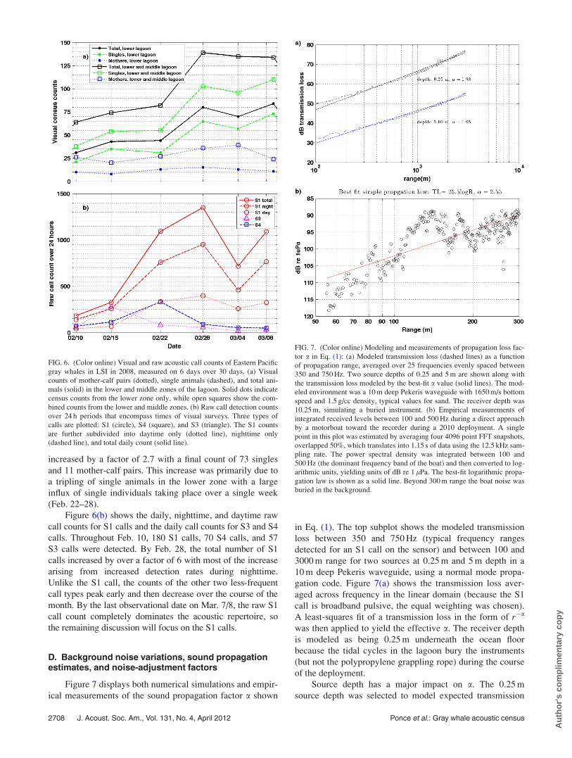
increased by a factor of 2.7 with a final count of 73 singles

and 11 mother-calf pairs. This increase was primarily due to

a tripling of single animals in the lower zone with a large

influx of single individuals taking place over a single week

(Feb. 22–28).

Figure 6(b) shows the daily, nighttime, and daytime raw

call counts for S1 calls and the daily call counts for S3 and S4

calls. Throughout Feb. 10, 180 S1 calls, 70 S4 calls, and 57

S3 calls were detected. By Feb. 28, the total number of S1

calls increased by over a factor of 6 with most of the increase

arising from increased detection rates during nighttime.

Unlike the S1 call, the counts of the other two less-frequent

call types peak early and then decrease over the course of the

month. By the last observational date on Mar. 7/8, the raw S1

call count completely dominates the acoustic repertoire, so

the remaining discussion will focus on the S1 calls.

D. Background noise variations, sound propagationestimates, and noise-adjustment factors

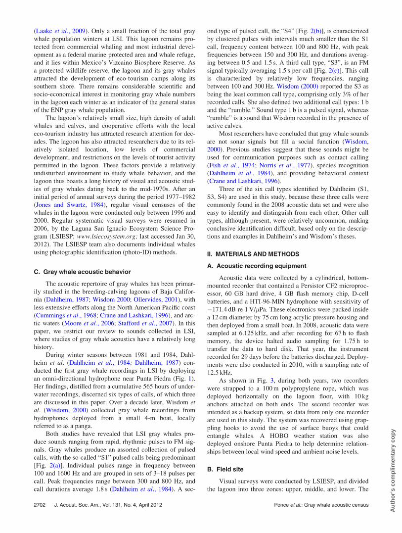
Figure 7 displays both numerical simulations and empir-

ical measurements of the sound propagation factor a shown

in Eq. (1). The top subplot shows the modeled transmission

loss between 350 and 750 Hz (typical frequency ranges

detected for an S1 call on the sensor) and between 100 and

3000 m range for two sources at 0.25 m and 5 m depth in a

10 m deep Pekeris waveguide, using a normal mode propa-

gation code. Figure 7(a) shows the transmission loss aver-

aged across frequency in the linear domain (because the S1

call is broadband pulsive, the equal weighting was chosen).

A least-squares fit of a transmission loss in the form of r�a

was then applied to yield the effective a. The receiver depth

is modeled as being 0.25 m underneath the ocean floor

because the tidal cycles in the lagoon bury the instruments

(but not the polypropylene grappling rope) during the course

of the deployment.

Source depth has a major impact on a. The 0.25 m

source depth was selected to model expected transmission

FIG. 6. (Color online) Visual and raw acoustic call counts of Eastern Pacific

gray whales in LSI in 2008, measured on 6 days over 30 days. (a) Visual

counts of mother-calf pairs (dotted), single animals (dashed), and total ani-

mals (solid) in the lower and middle zones of the lagoon. Solid dots indicate

census counts from the lower zone only, while open squares show the com-

bined counts from the lower and middle zones. (b) Raw call detection counts

over 24 h periods that encompass times of visual surveys. Three types of

calls are plotted: S1 (circle), S4 (square), and S3 (triangle). The S1 counts

are further subdivided into daytime only (dotted line), nighttime only

(dashed line), and total daily count (solid line).

FIG. 7. (Color online) Modeling and measurements of propagation loss fac-

tor a in Eq. (1): (a) Modeled transmission loss (dashed lines) as a function

of propagation range, averaged over 25 frequencies evenly spaced between

350 and 750 Hz. Two source depths of 0.25 and 5 m are shown along with

the transmission loss modeled by the best-fit a value (solid lines). The mod-

eled environment was a 10 m deep Pekeris waveguide with 1650 m/s bottom

speed and 1.5 g/cc density, typical values for sand. The receiver depth was

10.25 m, simulating a buried instrument. (b) Empirical measurements of

integrated received levels between 100 and 500 Hz during a direct approach

by a motorboat toward the recorder during a 2010 deployment. A single

point in this plot was estimated by averaging four 4096 point FFT snapshots,

overlapped 50%, which translates into 1.15 s of data using the 12.5 kHz sam-

pling rate. The power spectral density was integrated between 100 and

500 Hz (the dominant frequency band of the boat) and then converted to log-

arithmic units, yielding units of dB re 1 lPa. The best-fit logarithmic propa-

gation law is shown as a solid line. Beyond 300 m range the boat noise was

buried in the background.

2708 J. Acoust. Soc. Am., Vol. 131, No. 4, April 2012 Ponce et al.: Gray whale acoustic census

Au

tho

r's

com

plim

enta

ry c

op

y

loss from cavitation noise from small boats or animals vocal-

izing at or near the surface, while the 5 m source depth was

selected to represent a potential deeper depth for whale

vocalizations. The shallow depth yields a value of a close to

that expected by free-space spherical spreading; at a shallow

depth, the source excites mostly higher-order propagating

modes that suffer high attenuation loss through strong inter-

action with the ocean bottom. By contrast, sound from a

deeper source propagates more effectively through the water,

yielding a smaller value of a. Modeling sloping bathymetries

using gradients measured around Punta Piedra did not sub-

stantially change the value of a, but the simulations did not

incorporate potential acoustic backscatter from extremely

steep bathymetry gradients.

Unfortunately, high-quality empirical measurements of

propagation loss in the lagoon over the S1 call frequency

range are not available. While controlled playbacks of

sounds have been conducted in the lagoon by other research-

ers (Dahlheim, 1987, Appendix A), the playbacks occurred

at frequencies 1 kHz and higher, above the primary fre-

quency range of interest for the gray whale S1 call. Instead

empirical estimates of a have been obtained by using data

collected in 2010 to measure how the cavitation noise from a

research boat increases with decreasing range [Fig. 7(b)], as

the vessel directly approaches a recorder at the site with a

constant engine turnover. Figure 7(b) shows a value of a on

the order of 2.55, a value greater than the spherical spreading

prediction. This situation could arise if the source were

intrinsically directional or if a complicated bathymetry (such

as sand bars) created shadow zones and thus strong gradients

in transmission loss with range. To cover the full range of

possible a values in the LSI environment, propagation fac-

tors of 1.6 (from simulation, deeper whale call) and 2.55

(from boat measurements) will be used in the subsequent

sections.

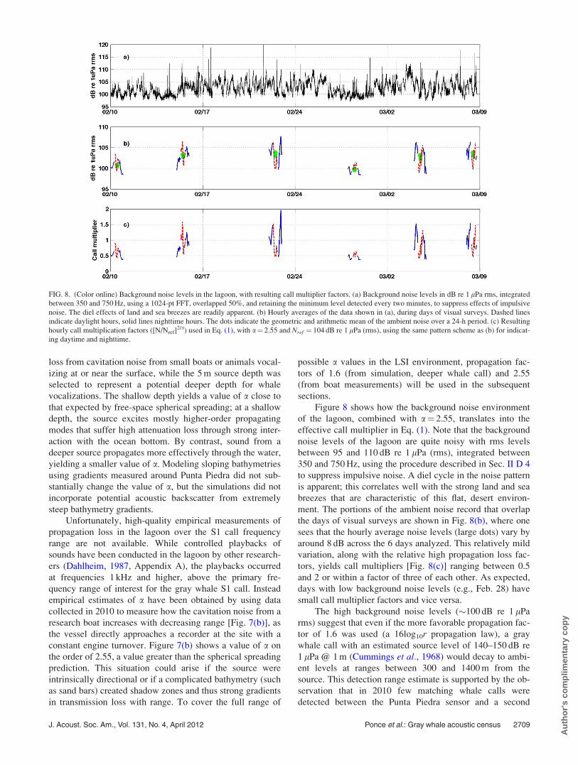
Figure 8 shows how the background noise environment

of the lagoon, combined with a¼ 2.55, translates into the

effective call multiplier in Eq. (1). Note that the background

noise levels of the lagoon are quite noisy with rms levels

between 95 and 110 dB re 1 lPa (rms), integrated between

350 and 750 Hz, using the procedure described in Sec. II D 4

to suppress impulsive noise. A diel cycle in the noise pattern

is apparent; this correlates well with the strong land and sea

breezes that are characteristic of this flat, desert environ-

ment. The portions of the ambient noise record that overlap

the days of visual surveys are shown in Fig. 8(b), where one

sees that the hourly average noise levels (large dots) vary by

around 8 dB across the 6 days analyzed. This relatively mild

variation, along with the relative high propagation loss fac-

tors, yields call multipliers [Fig. 8(c)] ranging between 0.5

and 2 or within a factor of three of each other. As expected,

days with low background noise levels (e.g., Feb. 28) have

small call multiplier factors and vice versa.

The high background noise levels (�100 dB re 1 lPa

rms) suggest that even if the more favorable propagation fac-

tor of 1.6 was used (a 16log10r propagation law), a gray

whale call with an estimated source level of 140–150 dB re

1 lPa @ 1 m (Cummings et al., 1968) would decay to ambi-

ent levels at ranges between 300 and 1400 m from the

source. This detection range estimate is supported by the ob-

servation that in 2010 few matching whale calls were

detected between the Punta Piedra sensor and a second

FIG. 8. (Color online) Background noise levels in the lagoon, with resulting call multiplier factors. (a) Background noise levels in dB re 1 lPa rms, integrated

between 350 and 750 Hz, using a 1024-pt FFT, overlapped 50%, and retaining the minimum level detected every two minutes, to suppress effects of impulsive

noise. The diel effects of land and sea breezes are readily apparent. (b) Hourly averages of the data shown in (a), during days of visual surveys. Dashed lines

indicate daylight hours, solid lines nighttime hours. The dots indicate the geometric and arithmetic mean of the ambient noise over a 24-h period. (c) Resulting

hourly call multiplication factors ([N/Nref]2/a) used in Eq. (1), with a¼ 2.55 and Nref ¼ 104 dB re 1 lPa (rms), using the same pattern scheme as (b) for indicat-

ing daytime and nighttime.

J. Acoust. Soc. Am., Vol. 131, No. 4, April 2012 Ponce et al.: Gray whale acoustic census 2709

Au

tho

r's

com

plim

enta

ry c

op

y

sensor placed 1.5 km away (Fig. 1). Thus the assumption

that the detection range of the sensor is not greater than the

width of the lagoon at Punta Piedra seems justified.

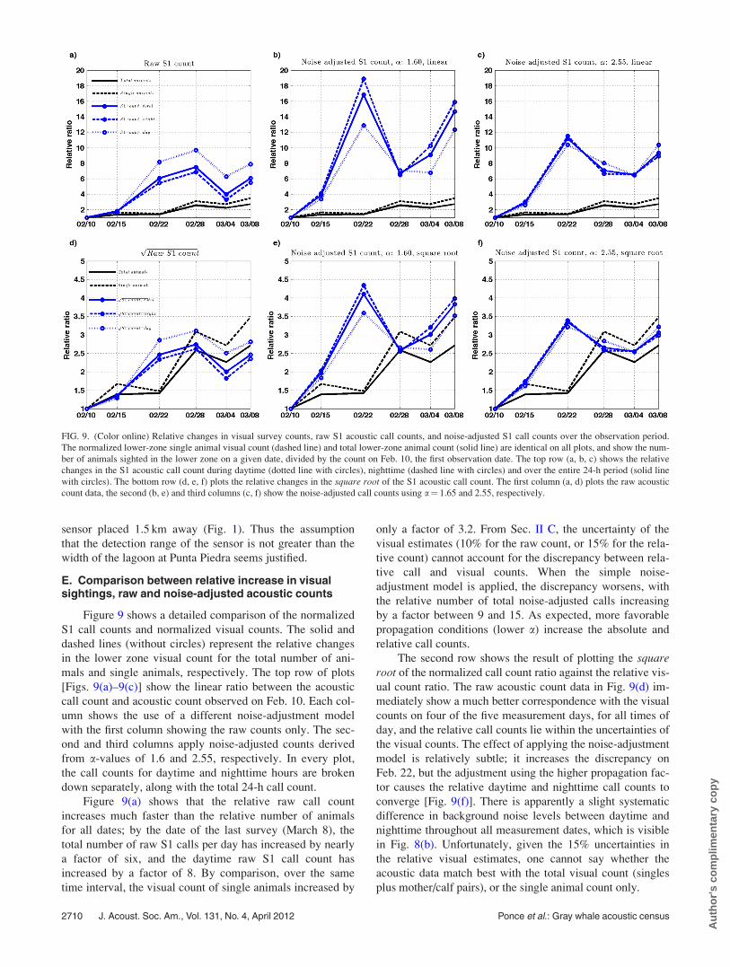
E. Comparison between relative increase in visualsightings, raw and noise-adjusted acoustic counts

Figure 9 shows a detailed comparison of the normalized

S1 call counts and normalized visual counts. The solid and

dashed lines (without circles) represent the relative changes

in the lower zone visual count for the total number of ani-

mals and single animals, respectively. The top row of plots

[Figs. 9(a)–9(c)] show the linear ratio between the acoustic

call count and acoustic count observed on Feb. 10. Each col-

umn shows the use of a different noise-adjustment model

with the first column showing the raw counts only. The sec-

ond and third columns apply noise-adjusted counts derived

from a-values of 1.6 and 2.55, respectively. In every plot,

the call counts for daytime and nighttime hours are broken

down separately, along with the total 24-h call count.

Figure 9(a) shows that the relative raw call count

increases much faster than the relative number of animals

for all dates; by the date of the last survey (March 8), the

total number of raw S1 calls per day has increased by nearly

a factor of six, and the daytime raw S1 call count has

increased by a factor of 8. By comparison, over the same

time interval, the visual count of single animals increased by

only a factor of 3.2. From Sec. II C, the uncertainty of the

visual estimates (10% for the raw count, or 15% for the rela-

tive count) cannot account for the discrepancy between rela-

tive call and visual counts. When the simple noise-

adjustment model is applied, the discrepancy worsens, with

the relative number of total noise-adjusted calls increasing

by a factor between 9 and 15. As expected, more favorable

propagation conditions (lower a) increase the absolute and

relative call counts.

The second row shows the result of plotting the squareroot of the normalized call count ratio against the relative vis-

ual count ratio. The raw acoustic count data in Fig. 9(d) im-

mediately show a much better correspondence with the visual

counts on four of the five measurement days, for all times of

day, and the relative call counts lie within the uncertainties of

the visual counts. The effect of applying the noise-adjustment

model is relatively subtle; it increases the discrepancy on

Feb. 22, but the adjustment using the higher propagation fac-

tor causes the relative daytime and nighttime call counts to

converge [Fig. 9(f)]. There is apparently a slight systematic

difference in background noise levels between daytime and

nighttime throughout all measurement dates, which is visible

in Fig. 8(b). Unfortunately, given the 15% uncertainties in

the relative visual estimates, one cannot say whether the

acoustic data match best with the total visual count (singles

plus mother/calf pairs), or the single animal count only.

FIG. 9. (Color online) Relative changes in visual survey counts, raw S1 acoustic call counts, and noise-adjusted S1 call counts over the observation period.

The normalized lower-zone single animal visual count (dashed line) and total lower-zone animal count (solid line) are identical on all plots, and show the num-

ber of animals sighted in the lower zone on a given date, divided by the count on Feb. 10, the first observation date. The top row (a, b, c) shows the relative

changes in the S1 acoustic call count during daytime (dotted line with circles), nighttime (dashed line with circles) and over the entire 24-h period (solid line

with circles). The bottom row (d, e, f) plots the relative changes in the square root of the S1 acoustic call count. The first column (a, d) plots the raw acoustic

count data, the second (b, e) and third columns (c, f) show the noise-adjusted call counts using a¼ 1.65 and 2.55, respectively.

2710 J. Acoust. Soc. Am., Vol. 131, No. 4, April 2012 Ponce et al.: Gray whale acoustic census

Au

tho

r's

com

plim

enta

ry c

op

y

Using the combined visual counts from the lower and

middle zone of the lagoon, instead of just the lower zone,

does not significantly change any of these results.

IV. DISCUSSION

A. Diel patterns in calling behavior

Bootstrap simulations and Welch’s t-tests have deter-

mined that S1 and S4 call detection rates are not uniformly

distributed over time (i.e., one can reject the null hypothesis

that the calls are generated uniformly and independently

with respect to time) and that the mean detection rates during

the day are lower than during the evening. To obtain these

conclusions for the S4 data, anomalously high call detection

rates between 16:00 and 18:00 on 2 days had to be removed.

One possible interpretation of this result is that gray

whales display a diel calling pattern for S1 and S4 calls—

which would be an unsurprising conclusion, given that con-

siderable literature already exists on diel patterns observed

in baleen whale call rates in ocean basins, including sei

(Baumgartner and Fratantoni, 2008), right (Munger et al.,2008), humpback (Au et al., 2000), and blue whales (Staf-

ford et al., 2005; Oleson et al., 2007). The peaking of call

rates at sunrise and sunset is also reminiscent of croaker fish

choruses along the eastern Pacific coast (D’Spain and Batch-

elor, 2006; Sirovic et al., 2009). The reason behind this pat-

tern is unknown; gray whales are not believed to feed during

the winter months in the lagoon.

Another potential contributing factor to the observed

diel pattern is that gray whales might become less vocal

whenever whale-watching tourist boat noise increases in the

lagoon (Ollervides, 2001) or from acoustic masking caused

by boats. For instance, the detection rates of S1 and S4 calls

dropped by 40% between 09:00 and 15:00 hours, which

coincide with the times of peak whale-watching activity

(Fig. 5). The next section examines this question in some

detail as well.

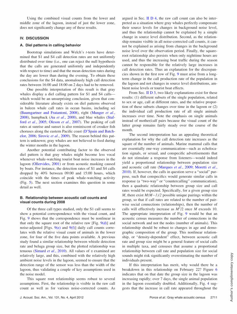
B. Relationship between acoustic call counts andvisual counts during 2008

Of the three call types studied, only the S1 call seems to

show a potential correspondence with the visual count, and

Fig. 9 shows that the correspondence must be nonlinear in

that only the square root of the relative raw [Fig. 9(d)] and

noise-adjusted [Figs. 9(e) and 9(f)] daily call counts corre-

lates with the relative visual count of animals in the lower

zone, for four of the five data points available. A previous

study found a similar relationship between whistle detection

rate and beluga group size, but the plotted relationship was

tenuous (Simard et al., 2010). All values of a examined are

relatively large, and this, combined with the relatively high

ambient noise levels in the lagoon, seemed to ensure that the

detection range of the sensor was less than the width of the

lagoon, thus validating a couple of key assumptions used in

the noise model.

This square root relationship seems robust to several

assumptions. First, the relationship is visible in the raw call

count as well as for various noise-corrected counts. As

argued in Sec. II D 4, the raw call count can also be inter-

preted as a situation where gray whales perfectly compensate

their source levels for changes in background noise level,

and thus the relationship cannot be explained by a simple

change in source level distribution. Second, as the relation-

ship remains visible in all noise-corrected call counts, it can-

not be explained as arising from changes in the background

noise level over the observation period. Finally, the square-

root relationship also persists when only nighttime hours are

used, and thus the increasing boat traffic during the season

cannot be responsible for the relatively large increases in

call detection rates. Thus an explanation for the discrepan-

cies shown in the first row of Fig. 9 must arise from a long-

term change in the call production rate of the population in

the lagoon and not changes in source level distributions, am-

bient noise levels or tourist boat effects.

From Sec. II D 3, two likely explanations exist for these

results: (1) different subsets of the single population, related

to sex or age, call at different rates, and the relative propor-

tion of these subsets changes over time in the lagoon or (2)

the individual call production rate of all single animals

increases over time. Note the emphasis on single animals

instead of mother/calf pairs because the visual count of the

latter group remains fairly steady over the course of the

month.

The second interpretation has an appealing theoretical

explanation for why the call detection rate increases as the

square of the number of animals. Marine mammal calls that

are essentially one-way communication—such as echoloca-

tion signals, or sexual, and conspecific advertisements that

do not stimulate a response from listeners—would indeed

yield a proportional relationship between population size

and acoustic call rate (Marques et al., 2009; Moretti et al.,2010). If, however, the calls in question serve a “social” pur-

pose, such that conspecifics would generate similar calls in

response (a “two-way” or “countercalling” communication),

then a quadratic relationship between group size and call

rates would be expected. Specifically, for a given group size

M, there exist M(M�1)/2 possible unique pairings within the

group, so that if call rates are related to the number of pair-

wise social connections (relationships), then the number of

calls will effectively increase as M2/2 once M exceeds 10.

The appropriate interpretation of Fig. 9 would be that an

acoustic census measures the number of connections in the

social network and not the nodes (number of animals). This

relationship should be robust to changes in age and demo-

graphic composition of the group. This nonlinear relation-

ship, or “density-dependent” effect, between acoustic call

rate and group size might be a general feature of social calls

in multiple taxa, and censuses that assume a proportional

relationship between call rate and population size for social

sounds might risk significantly overestimating the number of

individuals present.

If this interpretation has merit, why would there be a

breakdown in this relationship on February 22? Figure 6

indicates that on that date the group size in the lagoon was

increasing rapidly; over 7 days, the single animal population

in the lagoon essentially doubled. Additionally, Fig. 4 sug-

gests that the increase in call rate appeared throughout the

J. Acoust. Soc. Am., Vol. 131, No. 4, April 2012 Ponce et al.: Gray whale acoustic census 2711

Au

tho

r's

com

plim

enta

ry c

op

y

day, so the discrepancy cannot be explained by an increase

in call rates in the afternoon or evening, once the visual sur-

vey had been completed, or by a single whale persistently

vocalizing next to the hydrophone for several hours. Our ten-

tative interpretation is that whenever group size changes rap-

idly, individuals within the group become even more vocally

active than under “equilibrium” conditions. Once the group

size stabilizes, calling rates would gradually return to the

observed “square-root” equilibrium pattern. There is some

basis to this speculation; close-range acoustic and visual

observations of orcas in the Pacific Northwest found unusu-

ally heavy levels of acoustic activity from A-pod members,

when joined by resident whales from outside the same pod

(Ford, 1989).

V. CONCLUSION

A manual analysis has been conducted of acoustic call

rates of ENP gray whales residing in Laguna San Ignacio,

during 6 days over the course of the 2008 breeding season.

The analysis found evidence of a diel effect in call rates for

two call types, but it cannot be determined whether this cycle

arises from natural behavior or from peaks in noise from

boat activity during the afternoon.

The enclosed geography of the lagoon, combined with

the relatively short dive times of the animals, provided

excellent conditions for visual group size counts. The rela-

tively steady levels of ambient noise throughout the month,

combined with a large change in group size during the

month, permitted demonstration that over 4 of the 5 days an-

alyzed both the raw and noise-adjusted calling rates of a spe-

cific type of call (S1) were related to the square of the

number of animals in the lower zone of the lagoon. How-

ever, it was not possible to flag whether the relationship is

related to both demographic groups or just single, breeding

animals. The same relationship appeared during daytime and

nighttime hours, so an increase in tourism effects could not

be responsible for the observed relationship. We also note

that while this relationship is visible even without the noise-

adjustment model, the use of the model created greater con-

sistency between the relative increases predicted from call

counts measured during daytime and nighttime [Fig. 9(f)].

We interpret the observed nonlinear relationship as sug-

gesting that passive acoustic monitoring of social (two-way

communication) calls in gray whales does not measure popu-

lation size directly but instead measures the number of social

connections in the group. The exception to the observed rela-

tionship occurred during a time of rapid increase in the

whales’ group size in the lagoon, and it is speculated that

acoustic social calling rates will be poorly correlated with

group size during times of rapid change in whale group size.

The relationship between call rate and group size is

speculated to be a general feature of social sounds in multi-

ple taxa. Future work includes applying automated analysis

to all days of the acoustic record, repeating the analysis at

several locations around the lagoon, between years as well

as within years, and adding biopsy sampling to the LSIESP

research group, to allow quantifying the potential influences

of sex and age distribution on acoustic censusing efforts.

ACKNOWLEDGMENTS

Our appreciation is extended to Marilyn Dahlheim and

Sheyna Wisdom for providing useful information on gray

whale sounds and discussing their previous research in the

lagoon. Sheyna Wisdom also provided helpful comments on

the manuscript. We thank Delphine Mathias and the Laguna

San Ignacio Ecosystem Science Program (LSIESP) research-

ers Sergio Gonzalez C., Alejandro Gomez-Gallardo U.,

Benjamın Troyo V., Mauricio Najera C., Angie Sremba, and

Anaid Urban for their help in the field collecting visual data.

We also thank the managers, staff, and whale-watching boat

operators at Ecoturismo Kuyima for their hospitable services

during our fieldwork in Laguna San Ignacio. Robert Glatts

designed and assembled the acoustic recording devices, and

Dawn Grebner provided helpful references on killer whale

vocal behavior during merger groups. This research was con-

ducted under the supervision of Mexican research permit

No. 08433 from the “Subsecretaria de Gestion para la Pro-

teccion Ambiental, Direccion General de Vida Silvestre.”

Adi, K., Johnson, M. T., and Osiejuk, T. S. (2010). “Acoustic censusing

using automatic vocalization classification and identity recognition,” J.

Acoust. Soc. Am. 127, 874–883.

Au, W. W. L., Mobley, J., Burgess, W. C., Lammers, M. O., and Nachtigall,

P. E. (2000). “Seasonal and diurnal trends of chorusing humpback whales

wintering in waters off western Maui,” Marine Mammal Sci. 16, 530–544.

Baptista, L. F., and Gaunt, S. L. L. (1997). “Bioacoustics as a tool in conser-

vation studies,” in Behavioral Approaches to Conservation in the Wild,

edited by J. R. Clemmons, and R. Buchholz (Cambridge University Press,

Cambridge, MA), p. 404.

Baumgartner, M. F., and Fratantoni, D. M. (2008). “Diel periodicity in both

sei whale vocalization rates and the vertical migration of their copepod

prey observed from ocean gliders,” Limnol. Oceanogr. 53, 2197–2209.

Crane, N. L., and Lashkari, K. (1996). “Sound production of gray whales,

Eschrichtius robustus, along their migration route: A new approach to sig-

nal analysis,” J. Acoust. Soc. Am. 100, 1878–1886.

Cummings, W. C., Thompson, P. O., and Cook, R. (1968). “Underwater

sounds of migrating gray whales, Eschrichtius glaucus (Cope),” J. Acoust.

Soc. Am. 44, 1278–1281.

D’Spain, G. L., and Batchelor, H. H. (2006). “Observations of biological

choruses in the Southern California Bight: A chorus at midfrequencies,” J.

Acoust. Soc. Am. 120, 1942–1955.

Dahlheim, M. E. (1987). “Bio-acoustics of the gray whale (Eschrichtiusrobustus),” Ph.D. thesis, University of British Columbia, Canada.

Dahlheim, M. E., Fisher, H. D., and Schempp, J. D. (1984). “Sound produc-

tion by the gray whale and ambient noise levels in Laguna San Ignacio,

Baja California Sur, Mexico” in The Gray Whale, Eschrichtius robustus,edited by M. L. Jones, S. L. Swartz, and S. Leatherwood (Academic,

Orlando, FL), pp. 511–541.

Dawson, D. K., and Efford, M. G. (2009). “Bird population density esti-

mated from acoustic signals,” J. Appl. Ecol. 46, 1201–1209.

Douglas, L. (2000). “Click counting: An acoustic censusing method for esti-

mating sperm whale abundance,” Masters thesis, University of Otago.

Everest, F. A., Young, R. W., and Johnson, M. W. (1948). “Acoustical char-

acteristics of noise produced by snapping shrimp,” J. Acoust. Soc. Am. 20,

137–142.

Fish, J., Sumich, J. L., and Lingle, G. L. (1974). “Sound activity of the Cali-

fornia gray whale (Eschrictius robustus),” Mar. Fish. Rev. 36, p. 38–45.

Ford, J. K. B. (1989). “Acoustic behavior of resident killer whales (Orcinus-

Orca) off Vancouver Island, British–Columbia,” Can. J. Zool. 67,

727–745.

Henderson, D. A. (1984). “Nineteenth Century Gray Whaling: Grounds,

catches, and kills, practices and depletion of the whale population,” in TheGray Whale, Eschrichtius robustus, edited by M. L. Jones, S. L. Swartz,

and S. Leatherwood (Academic, Orlando, FL), pp. 159–186.

Jones, M. L., and Swartz, S. L. (1984). “Demography and phenology of gray

whales and evaluation of whale-watching activities in Laguna San Ignacio,

Baja California Sur, Mexico,” in The Gray Whale, Eschrichtius robustus,

2712 J. Acoust. Soc. Am., Vol. 131, No. 4, April 2012 Ponce et al.: Gray whale acoustic census

Au

tho

r's

com

plim

enta

ry c

op

y

edited by M. L. Jones, S. L. Swartz, and S. Leatherwood (Academic, Or-

lando, FL), pp. 309–374.

Kyhn, L. A., Tougaard, J., Thomas, L., Duve, L. R., Stenback, J., Amundin,

M., Desportes, G., and Teilmann, J. (2012). “From echolocation clicks to

animal density—Acoustic sampling of harbor porpoises with static data-

loggers,” J. Acoust. Soc. Am. 131, 550–560.

Laake, J., Punt, A., Hobbs, R., Ferguson, M., Rugh, D., and Briewick, J.

(2009). “Re-analysis of gray whale southbound migration surveys:

1967–2006,” Technical Mem. NMFS-AKFSC-203, (U.S. Dept. of

Commerce).

Marques, T. A., Thomas, L., Ward, J., DiMarzio, N., and Tyack, P. L.

(2009). “Estimating cetacean population density using fixed passive acous-

tic sensors: An example with Blainville’s beaked whales,” J. Acoust. Soc.

Am. 125, 1982–1994.

Mate, B. R., Lagerquist, B. A., and Urban-Ramirez, J. (2003). “A note on

using satellite telemetry to document the use of San Ignacio Lagoon by

gray whales (Eschrictius robustus) during their repordicutive season,” J.

Cetacean Res. Manage. 5, 149–154.

McDonald, M. A., and Fox, C. G. (1999). “Passive acoustic methods applied

to fin whale population density estimation,” J. Acoust. Soc. Am. 105,

2643–2651.

Mellinger, D. K., Nieukirk, S. L., Matsumoto, H., Heimlich, S. L., Dziak, R.

P., Haxel, J., Fowler, M., Meinig, C., and Miller, H. V. (2007a). “Seasonal

occurrence of North Atlantic right whale (Eubalaena glacialis) vocaliza-

tions at two sites on the Scotian Shelf,” Marine Mammal Sci. 23,

856–867.

Mellinger, D. K., Stafford, K. M., and Fox, C. G. (2004a). “Seasonal occur-

rence of sperm whale (Physeter macrocephalus) sounds in the Gulf of

Alaska, 1999–2001,” Marine Mammal Sci. 20, 48–62.

Mellinger, D. K., Stafford, K. M., Moore, S. E., Dziak, R. P., and Matsu-

moto, H. (2007b). “An overview of fixed passive acoustic observation

methods for cetaceans,” Oceanography 20, 36–45.

Mellinger, D. K., Stafford, K. M., Moore, S. E., Munger, U., and Fox, C. G.

(2004b). “Detection of North Pacific right whale (Eubalaena japonica)

calls in the Gulf of Alaska,” Marine Mammal Sci. 20, 872–879.

Moore, S. E., Stafford, K. M., Mellinger, D. K., and Hildebrand, J. A.

(2006). “Listening for large whales in the offshore waters of Alaska,” Bio-

science 56, 49–55.

Moretti, D., Marques, T. A., Thomas, L., DiMarzio, N., Dilley, A., Morris-

sey, R., McCarthy, E., Ward, J., and Jarvis, S. (2010). “A dive counting

density estimation method for Blainville’s beaked whale (Mesoplodondensirostris) using a bottom-mounted hydrophone field as applied to a

mid-frequency active (MFA) sonar operation,” Appl. Acoust. 71,

1036–1042.

Munger, L. M., Wiggins, S. M., Moore, S. E., and Hildebrand, J. A. (2008).

“North Pacific right whale (Eubalaena japonica) seasonal and diel calling

patterns from long-term acoustic recordings in the southeastern Bering

Sea, 2000–2006,” Marine Mammal Sci. 24, 795–814.

Noad, M. J., and Cato, D. H. (2000). “Comparison of acoustic and visual

surveying of humpback whales off East Australia,” J. Acoust. Soc. Am.

108, 2540.

Norris, K. S., Goodman, R. M., Villa-Ramirez, B., and Hobbs, L. (1977).

“Behavior of the California gray whale, Eschrichtius robustus, in southern

Baja California,” Fish. Bull. 75.

Oleson, E. M., Wiggins, S. M., and Hildebrand, J. A. (2007). “Temporal

separation of blue whale call types on a southern California feeding

ground,” Anim. Behav. 74, 881–894.

Ollervides, F. J. (2001). “Gray whales and boat traffic: movement, vocal,

and behavioral responses in Bahia Magdalena, Mexico,” Ph.D. thesis,

Texas A&M University.

Parks, S. E., Clark, C. W., and Tyack, P. L. (2007). “Short- and long-term

changes in right whale calling behavior: The potential effects of noise on

acoustic communication,” J. Acoust. Soc. Am. 122, 3725–3731.

Payne, K. B., Thompson, M., and Kramer, L. (2003). “Elephant calling pat-

terns as indicators of group size and composition: the basis for an acoustic

monitoring system,” Afr. J. Ecol. 41, 99–107.

Reeves, R. R., Smith, T. D., Lund, J. N., Lebo, S. A., and Josephson, E. A.

(2010). “Ninetheenth-century ship-based catches of gray whales, Eschrich-tius robustus, in the eastern North Pacific,” Marine Fish. Rev. 72, 26–65.

Rice, D. W., and Wolman, A. A. (1971). “The life history and ecology of

the gray whale (Eschrichtius robustus),” Special Publication Number 3,

(American Society of Mammalogists), p. 142.

Simard, Y., Roy, N., Giard, S., Gervaise, C., Conversano, M., and Menard,

N. (2010). “Estimating whale density from their whistling activity: Exam-

ple with St. Lawrence beluga,” Appl. Acoust. 71, 1081–1086.

Sirovic, A., Cutter, G. R., Butler, J. L., and Demer, D. A. (2009). “Rockfish

sounds and their potential use for population monitoring in the Southern

California Bight,” Ices J. Mar. Sci. 66, 981–990.

Stafford, K. M., Fox, C. G., and Clark, D. S. (1998). “Long-range acoustic

detection and localization of blue whale calls in the northeast Pacific

Ocean,” J. Acoust. Soc. Am. 104, 3616–3625.

Stafford, K. M., Moore, S. E., and Fox, C. G. (2005). “Diel variation in blue

whale calls recorded in the eastern tropical Pacific,” Anim. Behav. 69,

951–958.

Stafford, K. M., Moore, S. E., Spillane, M., and Wiggins, S. (2007). “Gray

whale calls recorded near barrow, Alaska, throughout the winter of 2003-

04,” Arctic 60, 167–172.

Thompson, M. E., Schwager, S. J., and Payne, K. B. (2010). “Heard but not

seen: an acoustic survey of the African forest elephant population at

Kakum Conservation Area, Ghana,” Afr. J. Ecol. 48, 224–231.

Urban, J., Gomez-Gallardo, A., Sahagun, F. d., Cifuentes, J., Ludwig, S.,

and Palmeros, M. (1997). “Gray whales at Laguna San Ignacio, B.C.S.

Mexico, Winter 1996,” Rep. Intl. Whal. Comm. 47, 625–633.

Urban, J. R., Rojas-Bracho, L., Perez-Cortez, H., Gomez-Gallardo, A.,

Swartz, S., Ludwig, S., and R. L. Brownell, J. (2003). “A review of gray

whales on their wintering grounds in Mexican waters,” J. Cetacean Res.

Manage. 5, 281–295.

Venter, P. J., and Hanekom, J. J. (2010). “Automatic detection of African

elephant (Loxodonta africana) infrasonic vocalisations from recordings,”

Biosyst. Eng. 106, 286–294.

Wisdom, S. (2000). “Sound production development in gray whales,” M.S.

thesis, University of San Diego.

J. Acoust. Soc. Am., Vol. 131, No. 4, April 2012 Ponce et al.: Gray whale acoustic census 2713

Au

tho

r's

com

plim

enta

ry c

op

y