DISCUSSION PAPER SERIES

ABCD

www.cepr.org

Available online at: www.cepr.org/pubs/dps/DP4431.asp www.ssrn.com/xxx/xxx/xxx

No. 4431

RELATIVE AND ABSOLUTE INCENTIVES: EVIDENCE ON

WORKER PRODUCTIVITY

Oriana Bandiera, Iwan Barankay and Imran Rasul

PUBLIC POLICY

ISSN 0265-8003

RELATIVE AND ABSOLUTE INCENTIVES: EVIDENCE ON

WORKER PRODUCTIVITY

Oriana Bandiera, London School of Economics (LSE) and CEPR Iwan Barankay, University of Essex

Imran Rasul, University of Chicago and CEPR

Discussion Paper No. 4431 June 2004

Centre for Economic Policy Research 90–98 Goswell Rd, London EC1V 7RR, UK

Tel: (44 20) 7878 2900, Fax: (44 20) 7878 2999 Email: cepr@cepr.org, Website: www.cepr.org

This Discussion Paper is issued under the auspices of the Centre’s research programme in PUBLIC POLICY. Any opinions expressed here are those of the author(s) and not those of the Centre for Economic Policy Research. Research disseminated by CEPR may include views on policy, but the Centre itself takes no institutional policy positions.

The Centre for Economic Policy Research was established in 1983 as a private educational charity, to promote independent analysis and public discussion of open economies and the relations among them. It is pluralist and non-partisan, bringing economic research to bear on the analysis of medium- and long-run policy questions. Institutional (core) finance for the Centre has been provided through major grants from the Economic and Social Research Council, under which an ESRC Resource Centre operates within CEPR; the Esmée Fairbairn Charitable Trust; and the Bank of England. These organizations do not give prior review to the Centre’s publications, nor do they necessarily endorse the views expressed therein.

These Discussion Papers often represent preliminary or incomplete work, circulated to encourage discussion and comment. Citation and use of such a paper should take account of its provisional character.

Copyright: Oriana Bandiera, Iwan Barankay and Imran Rasul

CEPR Discussion Paper No. 4431

June 2004

ABSTRACT

Relative and Absolute Incentives: Evidence on Worker Productivity*

We use personnel data to compare worker productivity under a relative incentive scheme, where worker pay is negatively related to the average productivity of co-workers, with productivity under piece rates – where pay is based on individual productivity alone. We find that for the average worker, productivity is at least 50% higher under piece rates. We show this is because workers partially internalize the negative externality they impose on others under the relative incentive scheme and do so to a greater extent when they work alongside their close friends. The results illustrate the importance of understanding how workers behave in the presence of externalities when designing incentive schemes.

JEL Classification: J33 and M52 Keywords: absolute incentives, relative incentives and social preferences

Oriana Bandiera Department of Economics London School of Economics Houghton Street LONDON WC2A 2AE Tel: (44 20) 7955 7519 Fax: (44 20) 7055 6951 Email: o.bandiera@lse.ac.uk For further Discussion Papers by this author see: www.cepr.org/pubs/new-dps/dplist.asp?authorid=147704

Iwan Barankay Department of Economics University of Essex Wivenhoe Park Colchester CO4 3SQ Tel: (44 1206) 872 729 Email: itbara@essex.ac.uk For further Discussion Papers by this author see: www.cepr.org/pubs/new-dps/dplist.asp?authorid=156718

Imran Rasul University of Chicago Graduate School of Business 1101 East 58th Street Chicago IL 60637 USA Tel: (1 773) 834 8690 Fax: (1 773) 702 0458 Email: imran.rasul@gsb.uchicago.edu For further Discussion Papers by this author see: www.cepr.org/pubs/new-dps/dplist.asp?authorid=157538

*We have benefited from discussions with Heski Bar-Isaac, V Baskar, Tim Besley, Marianne Bertrand, David Card, Chris Flinn, Ed Lazear, Alan Manning, Dilip Mookherjee, John Pencavel, Amil Petrin, Canice Prendergast, Matthew Rabin, Debraj Ray, and seminar participants at Berkeley, Boston University, Chicago GSB, Columbia, Essex, Georgetown, IUPUI, LSE, NYU, Stanford, Toronto, Warwick, and Yale. The research started when the first author was visiting the GSB at the University of Chicago, whom she thanks for their hospitality. Financial support from the RES and STICERD is gratefully acknowledged. We are indebted to all those involved in providing the data. This Paper has been screened to ensure no confidential data are revealed. All errors remain our own.

Submitted 16 April 2004

1 Introduction

This paper uses personnel data to compare the effect of relative and absolute incentive schemes

on workers’ productivity. Relative schemes - where an individual’s reward depends on her per-

formance relative to others’ in her peer group - are ubiquitous in society and the focus of an

extensive theoretical literature. Their effect on productivity in the workplace, however, remains

largely unknown.1

One key difference between relative and absolute incentive schemes is that under relative

incentives, individual effort imposes a negative externality on co-workers by lowering their relative

performance, and hence their pay. Under piece rates, in contrast, individual reward depends only

on individual performance and so individual effort has no effect on others’ pay.

Understanding the extent to which workers internalize the externality is crucial for the optimal

choice between relative and absolute incentive schemes. Theoretical comparisons of relative and

absolute schemes generally rely on the assumptions that workers cannot cooperate and they

ignore the externality when choosing their effort. We investigate whether this assumption is

borne out in the data, thus providing real world evidence on individual behavior in a situation

where individual and social optima do not coincide.

We use personnel data from a leading UK farm that first used a relative incentive scheme for

its workers, and then moved to piece rates. The workers’ task is to pick fruit and their individual

productivity is recorded daily. Under the relative incentive scheme, workers’ daily pay depends

on the ratio of individual productivity to average productivity among all co-workers in a field

on that day. Under the absolute incentive scheme - piece rates - individual pay only depends on

individual productivity.

The difference in worker productivity under the two schemes then critically depends on the

extent to which, if any, workers internalize the externality their effort has on the pay of their

co-workers. This, in turn, might depend on the relationship between co-workers. To address this

issue, we combine the personnel records with survey data that contains precise information on

each worker’s social network of friends on the farm.1This paper provides the first evidence on the comparison of absolute and relative incentive schemes in the

workplace. Knoeber and Thurman (1994) analyze the effects of two different relative incentive schemes on chickenranchers. The theory of rank order tournaments - a type of relative incentive - has been tested in experimentaldata (Bull et al (1987)) and in sports tournaments (Ehrenberg and Bognanno (1990), Becker and Huselid (1992)).Lazear (2000), Paarsch and Shearer (1996) and Shearer (2004) show that incentives matter per se - they findsizeable gains in worker productivity when moving from fixed pay to piece rates. Similarly, Laffont and Matoussi(1995) find worker productivity to be 50% higher in farms operated under high powered (fixed rent) contractscompared to those operated under low powered (sharecropping) contracts. Finally, Foster and Rosenzweig (1994)show that effort, proxied by the depletion of BMI net of calorie intake, is 22% higher for rural laborers paidby piece rates compared to those paid hourly wages. See Prendergast (1999) for a review of the literature onincentives.

2

Four features of the data help identify the causal effect of the change in incentive schemes and

of group composition on worker productivity. First, we use information on the daily productivity

of the same workers before and after the introduction of piece rates. Time invariant sources of

unobservable individual heterogeneity are therefore controlled for.2

Second, there is no endogenous sorting of new workers into the sample and no endogenous

attrition of workers out of the sample, at the time of the change in incentive schemes.3

Third, the change in incentive scheme was announced on the day it was implemented and other

farm practices remained unchanged throughout the season. Tasks, technology and management

were the same under both incentives schemes.

Finally, the group co-workers each individual works with changes daily. This allows us to

identify the effect of group composition on worker productivity from the comparison of the

behavior of the same worker working alongside different co-workers.

We find the change in incentive schemes had a significant and permanent impact on produc-

tivity. For the average worker, productivity increased by 50% moving from relative incentives to

piece rates. The result is robust to controlling for a host of time varying factors at the worker,

field, and farm level. Moreover, the increase in productivity did not come at the expense of a

lower quality of fruit picking.

To shed light on the workers’ maximization problem, we calibrate the first order conditions

for worker’s effort choice under alternative behavioral assumptions. This exercise reveals that the

observed change in productivity is too large to be consistent with the Nash equilibrium outcome

where workers maximize their individual net benefit and ignore the externality they impose on

others. However, workers’ behavior under relative incentives is also not consistent with the

assumption that workers maximize the group’s welfare. Namely, effort levels are too high under

relative incentives to be consistent with workers fully internalizing the negative externality their

effort imposes on others.

We then posit that workers place some weight on the payoffs accruing to their co-workers.

Such social preferences can be thought as a reduced form representation of altruism or of collusive

behavior. Our setting exhibits several features that facilitate collusion. Workers can monitor

each other easily, they work with one another frequently and live on the farm together, implying

that social sanctions can be used as a punishment mechanism.

2This is in contrast to studies that use cross-sectional variation across firms to measure incentive effects. Ifworkers are not randomly allocated across firms, unobserved worker heterogeneity biases such estimates of theeffect of incentives on productivity.

3This is important given existing evidence suggesting the quantitative effects on productivity of the endogenoussorting of workers in response to a change in incentives are at least as strong as those arising from the incentivesdirectly. Lazear (2000) uses worker level data to analyze the effect on installers of auto windshields of movingfrom fixed wage contracts to piece rates. He finds an increase in productivity of 44% six months after the changein incentives. Half of this is attributed to the endogenous turnover of workers.

3

We find that workers internalize the negative externality their effort imposes on others to

some extent. The observed change in productivity is consistent with the average worker placing

a weight of .65 on the benefits accruing to all other co-workers, assuming they place a weight of

one on their own benefits.4

Further analysis reveals that the extent to which workers internalize the externality depends

on their relationship with their group of co-workers. Under relative incentives workers are sig-

nificantly less productive when the share of their personal friends in the group is larger and this

effect is stronger in smaller groups. In contrast, we find that productivity under piece rates is

not affected by the relationships among co-workers.

Overall our findings imply worker productivity is significantly different under the two schemes

because workers internalize the externality they impose on others under relative incentives, and

they do so more when they work alongside friends.

In addition to explaining why relative incentives performed so poorly in this setting, our

findings also imply that group incentives, namely schemes where individual pay is positively

linked to the group’s productivity, outperform piece rates when workers have social preferences,

other things equal. The fact that workers internalize the externality they impose on others thus

provides a rationale for group incentives even in settings where the production technology does

not exhibit complementarities. Overall, the results demonstrate the importance of understanding

how workers behave in the presence of externalities when designing incentive schemes.

The paper is organized into 7 sections. Section 2 sets out stylized models of worker’s effort

choices under alternative behavioral assumptions. Section 3 describes the data. Section 4 presents

estimates of the causal effect of the change in incentives on productivity. Section 5 brings

alternative models of workers’ behavior to the data. Section 6 analyzes the effect of the identity

of co-workers on productivity under the two incentive schemes. Section 7 concludes with a

discussion on the design of incentive schemes when workers have social preferences. The appendix

contains additional regression results.

2 Theoretical Framework

This section makes precise the workers’ effort choice under relative incentives and under piece

rates. Consider a group ofN workers. Each worker i exerts ei ≥ 0 units of effort which determinesher productivity. Without loss of generality, we assume that effort equals productivity in what

follows. Each worker’s payoff is φ (.) − θie2i

2, where φ (.) is the benefit derived from pay (which

4Our findings are in line with the large experimental literature on public good games where individual con-tributions are generally found to be halfway between the selfish Nash equilibrium (complete free riding) and thegroup optimum (Ledyard (1995)).

4

depends on effort), and θie2i2is the cost of effort. We assume φ (.) is a differentiable concave

function, with limx→0 φ0 (x) =∞. The parameter θi is interpreted as the inverse of the workersinnate ability. We assume workers are heterogeneous along this dimension, and can be ordered

such that θ1 < θ2 < ... < θN , where θi > 0 for all i.

The relationship between effort and pay depends on the incentive scheme as explained below.

Relative Incentives

Under the relative incentive scheme observed in the data, each worker’s pay depends on how

she performs relative to her peers. More specifically, workers’ benefit from pay takes the form

φ¡eie

¢for all i, where e = 1

N

Pi ei is the average effort of all N workers.5 The relative scheme

has the key characteristics that other things equal, an increase in worker i’s effort - (i) increases

her pay; (ii) increases average effort and hence reduces the pay of everybody else in the group.

Hence each worker’s effort imposes a negative externality on the entire group of co-workers.

The choice of effort under relative incentives then depends on whether and to what extent workers

internalize this externality.

To this purpose, we assume workers have “social preferences”, namely they take into account

the effect of their effort on the benefits accruing to co-workers. If each worker places a social

weight, πi, on each of her fellow co-worker’s payoffs, the equilibrium effort for worker i solves;

maxei

φ³eie

´+ πi

Pj 6=i

µφ³eje

´− θje

2j

2

¶− θie

2i

2(1)

Such social preferences can be thought of as a reduced form representation of a number of

models. They depict behavior consistent with reciprocity or altruism (Fehr and Schmidt (1999)),

or the evolutionary equilibrium of a repeated Prisoner’s Dilemma game in which workers learn

which strategies to play (Levine and Pesendorfer (2002), Sethi and Somanathan (1999)). We do

not attempt to distinguish between models in which workers’ preferences display altruism towards

others, and models in which workers behave as if they are altruistic because, for instance, they

play trigger strategies to enforce collusive agreements.

Assuming worker i chooses her effort taking the effort of others as given, the Nash equilibrium

effort for worker i solves;

φ0³eie

´ 1e

µPj 6=i ej

(P

i ei)

¶− πi

e

Xj 6=i

φ0³eje

´ ej(P

i ei)= θiei (2)

5This relative incentive scheme is not a rank order tournament. Worker benefits are based on their cardinaland not their ordinal ranking. It is however similar to a “linear relative performance evaluation” (LRPE) schemeas studied in Knoeber and Thurman (1994). Under a LRPE worker’s compensation is, α + µ (ei − e), where αand µ are parameters taken as given by workers.

5

Piece Rates

Under piece rates, individual effort is paid at a fixed rate β per unit. With social preferences,

worker i chooses her effort under piece rates as follows;

maxei

φ (βei) + πiPj 6=i

µφ (βej)−

θje2j

2

¶− θie

2i

2(3)

The equilibrium effort level solves the first order condition;

φ0 (βei) β = θiei (4)

Naturally as worker i’s effort does not affect the pay of her co-workers, her optimal choice of

effort is independent of the social weight she places on others.

Comparing Relative Incentives and Piece Rates

To compare effort choices under the relative scheme and under piece rates we evaluate the

first order condition (4) at β = 1eso that for a given average effort level, the pay per unit of effort

is the same under both incentive schemes. The first order condition under piece rates then is;

φ0³eie

´ 1e= θiei (5)

The differences between the first order conditions (2) and (5) can then be ascribed to two

sources, both of which make effort levels under relative incentives lower than under piece rates.

The first and most important difference is the externality worker i imposes on others by in-

creasing her effort, therefore increasing the average effort and reducing the pay of co-workers un-

der relative incentives. The magnitude of this effect depends on the extent to which workers inter-

nalize the externality, that is, on the social weight πi. This is captured in the πie

Xj 6=i

φ0¡eje

¢ ej

(P

i ei)

term in (2).

Second, by exerting more effort, each worker lowers the pay she receives for each unit of effort

under relative incentives. This effect, captured by the termP

j 6=i ej(P

i ei), is negligible in large groups

as limN→∞P

j 6=i ej(P

i ei)= 1.6 7

6This is seen most clearly in the case of homogeneous workers. Then the Nash equilibrium effort level under

relative incentives is e∗i = eR =q¡1− 1

N

¢φ0 (1) and e∗i = eP =

pφ0 (1) under piece rates. The ratio of effort

under the two systems is thusq¡1− 1

N

¢. If workers are heterogeneous the ratio depends on group size and

workers’ ability, although it can be shown that limN→∞eR = eP .7In a dynamic framework, workers may underperform under piece rates to ensure management does not lower

the piece rate in future periods. This ratchet effect does not arise under relative incentives since the rate is setdaily based on average effort that day. The ratchet effect thus lowers effort under piece rates compared to relativeincentives. We discuss some the empirical implications of the ratchet effect in section 4.

6

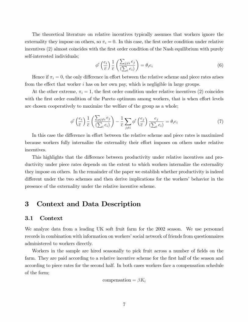
The theoretical literature on relative incentives typically assumes that workers ignore the

externality they impose on others, so πi = 0. In this case, the first order condition under relative

incentives (2) almost coincides with the first order condition of the Nash equilibrium with purely

self-interested individuals;

φ0³eie

´ 1e

µPj 6=i ej

(P

i ei)

¶= θiei (6)

Hence if πi = 0, the only difference in effort between the relative scheme and piece rates arises

from the effect that worker i has on her own pay, which is negligible in large groups.

At the other extreme, πi = 1, the first order condition under relative incentives (2) coincides

with the first order condition of the Pareto optimum among workers, that is when effort levels

are chosen cooperatively to maximize the welfare of the group as a whole;

φ0³eie

´ 1e

µPj 6=i ej

(P

i ei)

¶− 1

e

Xj 6=i

φ0³eje

´ ej(P

i ei)= θiei (7)

In this case the difference in effort between the relative scheme and piece rates is maximized

because workers fully internalize the externality their effort imposes on others under relative

incentives.

This highlights that the difference between productivity under relative incentives and pro-

ductivity under piece rates depends on the extent to which workers internalize the externality

they impose on others. In the remainder of the paper we establish whether productivity is indeed

different under the two schemes and then derive implications for the workers’ behavior in the

presence of the externality under the relative incentive scheme.

3 Context and Data Description

3.1 Context

We analyze data from a leading UK soft fruit farm for the 2002 season. We use personnel

records in combination with information on workers’ social network of friends from questionnaires

administered to workers directly.

Workers in the sample are hired seasonally to pick fruit across a number of fields on the

farm. They are paid according to a relative incentive scheme for the first half of the season and

according to piece rates for the second half. In both cases workers face a compensation schedule

of the form;

compensation = βKi

7

where Ki is the total kilograms of fruit picked by worker i in the day.8 Throughout we define

individual productivity yi as the number of kilograms of fruit picked per hour.

Under the relative scheme, the picking rate β is endogenously determined by the average

productivity of all workers in the field-day. In particular β is set equal to;

β =w

y(8)

where w is the minimum wage plus a positive constant fixed by the management at the beginning

of the season, and y is the average hourly productivity of all workers on the field-day. At the start

of each field-day, the field supervisor announces an ex ante picking rate based on her expectation

of worker productivity. This picking rate is revised at the end of each field-day to ensure a worker

with productivity y earns the pre-established hourly wage, w.

In line with the relative scheme analyzed in section 2, worker i’s compensation depends on

her productivity relative to the average productivity of her co-workers. In particular, given that

Ki = yih, where h is the number of hours worked in a day, worker i’s pay isyiyhw. Note that an

increase in worker i’s effort increases the average productivity on the field-day and thus imposes

a negative externality on her co-workers by reducing the picking rate β in (8).

Under piece rates, the picking rate is set ex ante, based on the supervisor’s expectation of

productivity that field-day, and is not revised.9 The key difference between the two systems is

that under the relative incentives, workers’ effort determines the rate at which they are paid,

whereas under piece rates it does not.10

Workers in the sample are hired on a casual basis, namely work is offered daily with no

guarantee of further employment. The majority of workers are hired from Eastern and Central

Europe and live together on the farm for the duration of their stay.11 Workers are issued with a

farm-specific work permit for a maximum of six months, implying they cannot be legally employed

8To comply with minimum wage laws, workers’ compensation is supplemented whenever βKi falls below thepro-rata minimum wage. In practice the farm management makes clear that any worker who needs to have theircompensation increased to the minimum wage level repeatedly would be fired. Indeed, we observe less than 1%of all worker-field-day observations involving pay increases to meet the minimum wage requirements. Of these,46% occurred under relative incentives, 54% occurred under piece rates.

9The data under piece rates indicates that the rate was set correctly in the sense that the ex ante rate underpiece rates is very close to the rate that would obtain ex post if the relative formula were used instead.10Workers face more uncertainty over the picking rate under relative incentives because although a rate is

announced ex ante, this can be revised ex post to reflect the productivity of the average worker. Under piecerates, the ex ante picking rate cannot be revised. However, uncertainty is unlikely to have a large impact on effortchoices because workers play the same game daily and have many opportunities to learn the ex post adjustmentof the picking rate under relative incentives. In section 4 we further discuss whether uncertainty can explain thechange in productivity we observe in the data.11In order to qualify, individuals must be full-time students, and having at least one year before graduation.

Workers must - (i) return to the same university in the autumn; (ii) be able to speak English; (iii) have notworked in the UK before; (iv) be aged between 19 and 25.

8

elsewhere in the UK. Their outside option is therefore to return to their home countries. The

vast majority of workers in the sample report their main reason to seek temporary employment in

the UK to be financial, which is hardly surprising in light of the fact that, even at the minimum

wage, the value of their earnings is high in real terms.12

We analyze productivity data on one type of fruit only and focus on the season’s peak time -

between midMay and the end of August. Data on workers’ productivity is recorded electronically.

Each worker is assigned a unique bar code, which is used to track the quantity of fruit they pick

on each field and day in which they work. This ensures little or no measurement error in recorded

productivity.

The sample is restricted to those workers who worked at least 10 field-days under each in-

centive scheme. Our working sample contains 10215 worker-field-day level observations, covering

142 workers, 22 fields and 108 days in total.

The incentive scheme changed midway through the season. Relative incentives were in place

for the first 54 days, piece rates were in place for the remaining 54.13 The change was announced

on the same day it was first implemented. No other organizational change took place during the

season, as reported by farm management and as documented in the next section.

Finally, interviews with the management reveal that the relative incentive scheme was adopted

because it allowed to difference out common productivity shocks, such as those deriving from

weather and field conditions, that are a key determinant of productivity in this setting. The

management eventually decided to move to piece rates because they believed productivity could

be higher. Whether the move to piece rates had the desired effect is analyzed in section 4.

3.2 Descriptive Analysis

Worker Productivity

Table 1 gives unconditional worker productivity by incentive scheme. Productivity rose sig-

nificantly from an average of 5.01kg/hr in the first half of the picking season under relative

incentives to 7.98kg/hr in the second half of the season under piece rates, an unconditional

increase in productivity of 59%.

Figures 1 and 2 show disaggregated productivity data across time and across workers under

the two schemes. Figure 1 shows the mean of worker productivity over time in the two fields that

were operated for the most days under each incentive scheme. Together these fields contribute one

12Working eight hours at the minimum wage rate implies a daily income of around 55 USD or 14300 USDper year (based on a five-day week). PPP adjusted GDP per capita is 3816 USD in the poorest of the samplecountries (Ukraine) and 11243 USD in the richest (Slovakia).13No picking takes place on Sundays. The panel is unbalanced in that we do not observe each worker picking

every day. This is of concern if there is endogenous attrition of either fields or workers over time. The empiricalanalysis in section 4 takes these concerns into account.

9

third of the total worker-field-day observations. Under relative incentives, there is no discernible

trend in productivity. With the introduction of piece rates, productivity rose and remained at a

higher level until the end of the season.

Figure 2 shows kernel density estimates of productivity by each incentive scheme. The pro-

ductivity of each of the 142 workers in the sample is averaged within each incentive scheme in

this figure. The mean and variance of productivity both rise moving from relative incentives to

piece rates.

Productivity is computed as kilograms picked per hour. The second and third rows of table

1 reveal that the increase in productivity was entirely due to workers picking more fruit over

the same time period, rather than working shorter hours. On average, workers picked 23.2 more

kilograms per day under piece rates - a significant difference at the 1% level. Hours worked did

not significantly change across incentive schemes.14

The discussion in section 2 makes clear that the size of the group over which relative pay is

computed is key for understanding workers’ behavior under relative incentives. The fourth row

of table 1 reports average group size, namely the number of people each worker worked with on a

given field and day. We note that average group size remained constant throughout the season.

Importantly, the fact that, on average, there are over 40 workers picking together under the

relative incentive scheme indicates that - (i) by exerting effort, the worker reduces the relative

performance of a large number of co-workers; (ii) the effect each worker has on her own pay is

negligible.

Aggregate Farm Level Data

Figure 3 shows the cumulative distributions of arrivals and departures of workers over the

season. The change in incentive scheme did not coincide with a wave of new arrivals, nor did it

hasten the departure of workers. Indeed, very few workers left before or just after the change in

incentive schemes.15

Figures 4a to 4c show total kilograms picked, total man-hours worked, and the total number

of pickers over the season at the level of the farm. Each series is measured as a percentage

deviation from its mean.

Kilograms picked per day shows no discernible trend under either incentive scheme.16 Total

man-hours spent picking are higher under relative incentives. Figure 4c shows this is due entirely

14Productivity levels in the first half of the 2003 season, when piece rates were in place throughout, are similarto those observed in the second half of the 2002 season. In the second half of the 2003 season a bonus schemewas introduced for field supervisors.15The cumulative distributions of arrivals and departures of workers in 2003 are similar to those in figure 3.16Given the farm faces a relatively constant product demand and labor supply through the season, there is

a deliberate timing of planting of fields to ensure that not all fruit ripens simultaneously. This smooths outvariations in productivity over time.

10

to more workers picking, rather than each worker picking for longer hours. The total man-hours

spent picking however falls as fewer workers are required to pick each day.

Figures 4a to 4c together indicate that while total kilograms picked and the time spent picking

per field-day remained constant throughout the season, the total number of workers allocated to

picking fell moving from relative incentives to piece rates.

Under piece rates, the management had some workers pick less frequently and instead had

them perform other tasks, mostly related to the transportation and packaging of fruit. These

workers had the same productivity as workers who continued regularly on picking tasks. They

also did not differ on characteristics such as gender and nationality.

Picking Rate and Daily Pay

Figure 5a shows the picking rate paid per kilogram over time, as a percentage deviation from

its mean. Under relative incentives the picking rate rises gradually as productivity declines. This

is as expected given that under the relative incentive scheme, the picking rate is set endogenously

according to (8).

With the introduction of piece rates there is a one-off fall in the picking rate. Table 1 shows

that the difference in average picking rates between the two halves of the season is significant at

the 1% level. We therefore rule out that the observed rise in productivity is a consequence of

higher returns to the marginal unit of effort under piece rates. To the contrary, the pay per unit

of effort is lower under piece rates.

Figure 5b then shows the daily pay from picking over the season, as a percentage deviation

from its mean. Given that productivity and picking rates are inversely related to each other,

average workers’ pay remained relatively constant over time. Table 1 shows that the difference

in average daily pay between relative incentives and piece rate is positive but not significantly

different from zero. Overall, the average worker became worse off under piece rates - their

productivity rose, while total compensation did not increase significantly. The estimates therefore

provide a lower bound of the effect of the change in incentives on productivity holding utility

constant.17 However, the top third of workers did have significant increases in pay moving to

piece rates (not reported), which is as expected if workers are of heterogeneous ability.

17We maintain the standard assumption in the incentive literature that the utility maximizing level of effortis increasing in the piece rate. We discuss whether income effects or income targeting can explain the observedincrease in productivity in section 4.

11

4 Evidence on Workers’ Productivity

4.1 Empirical Method

We assume the underlying production technology is Cobb Douglas, and estimate the productivity

of worker i on field f on day t, yift, using the following panel data regression, where all continuous

variables are in logarithms;

yift = αi + βf + γPt + δXift + ηZft + uift (9)

Worker fixed effects, αi, capture time invariant worker level determinants of productivity such as

innate ability and intrinsic motivation. Field fixed effects, βf , capture time invariant field level

determinants of productivity such as soil quality and fruit variety.

Pt is a dummy equal to one when piece rates are in place and zero when relative incentives

are in place. As piece rates are introduced simultaneously across all fields it is not possible to

control for day fixed effects. Instead we control for time varying factors at both the individual

and field level, in Xift and Zft respectively.

The disturbance term, uift, captures unobservable determinants of productivity at the worker-

field-day level. Worker observations within the same field-day are unlikely to be independent since

workers face similar field conditions. We account for this by clustering standard errors at the

field-day level in all productivity regressions.

The parameter of interest throughout is γ. There are three types of concerns that lead to γ

being inconsistently estimated.

First, as the change in incentive scheme occurs at the same time in all fields, identification of

the effect of incentives on productivity arises from a comparison over time of the same worker.

The estimated effect of piece rates, bγ, is then biased upward to the extent that it captures factorsthat cause productivity to rise through the season regardless of the change in incentive schemes.

This concern arises if, for instance, there is attrition of low yield fields over time.

Second, after the introduction of piece rates fewer workers were needed to pick the same

amount of fruit. The estimate bγ can be biased if the composition of tasks a worker performs ona given day affects productivity, if the selection of workers out of picking was related to their

productivity, and if the identity of co-workers affects individual productivity.

Third, both the timing of the change in incentives, and the response of workers before or

after the change may be endogenous. For instance, if management shifted to piece rates when

productivity under relative incentives was at its lowest, bγ is biased upwards. If on the otherhand, workers initially under perform under piece rates in the hope of reinstating the relative

incentive scheme, bγ is biased downwards.12

We address these issues in the next section after presenting the baseline estimates of (9).

4.2 Results

Table 2 presents the baseline estimates of the causal effect of the change in incentive scheme on

worker productivity. Column 1 regresses worker productivity on a dummy for the introduction

of the piece rate, clustering standard errors by field-day. Productivity significantly rises by 53%

when moving from relative incentives to piece rates.18

Column 2 controls for worker fixed effects, so that only variation within a worker over time is

exploited, while column 3 also adds field fixed effects, so only variation within a worker picking on

the same field over time is exploited. The coefficient of interest remains significant and of similar

magnitude. Controlling for worker heterogeneity improves the fit of the model considerably -

workers fixed effects almost double the explained variation in productivity. In contrast, field

heterogeneity appears to be much less important.

Column 4 controls for other time varying determinants of productivity at the level of the

farm, field, and individual. We include a linear time trend to capture farm level changes over

time, a measure of each field’s life cycle to capture field level changes over time and a measure

of each worker’s picking experience.

We measure the field’s life cycle as the number of days that the field has been operated at

any moment in time, divided by the total number of days that the field is operated over the

season. Picking experience is defined as the number of field-days the worker has picked for.19

There is no trend in productivity over time at the level of the farm, all else equal. This is

consistent with the fact that different fields are operated at different times to ensure a constant

stream of output throughout the season. Within each field however, productivity declines as the

field is picked later in its cycle. Moreover, there are positive returns to picking experience as

expected.20

A one standard deviation increase in the field life cycle reduces productivity by 20%, while a

one standard deviation increase in picking experience increases productivity by 7%. In compar-

18We experimented with a number of alternative specifications for calculating standard errors. First we allowedobservations to be clustered at the worker level to account for idiosyncratic worker characteristics that lead toworker productivity over different days being correlated. Doing so caused standard errors to fall relative to thosein column 1. Second, we also ignored time variation altogether and collapsed the data into a single observation foreach worker under each incentive scheme. Doing so, we continued to find that productivity increases significantly,at the 1% level after the change in incentive scheme. This and other results not reported for reasons of space areavailable upon request.19Management informed us that it takes a worker between 6 and 10 days before they are able to pick at their

optimal speed. For the first 4 days they pick, workers are paid an hourly wage. This initial period of learning isnot in our sample.20Defining work experience as the cumulative hours spent picking also led to similar results as those reported.

13

ison, the introduction of piece rates causes productivity to significantly increase by 58%.

Further analysis, not reported for reasons of space, show that this result is robust to control-

ling for other time varying factors including contemporaneous and lagged weather conditions,

field supervisor fixed effects, and the ratio of supervisors to workers.21

Spurious Time Effects

As the change in incentive scheme occurs at the same time in all fields, identification of the

effect of incentives on productivity arises from a comparison of the same worker over time. The

estimated effect of piece rates bγ is biased upward if it captures the effect of factors that causeproductivity to rise through the season regardless of the change in incentive schemes.

The first two columns of table 3 estimate the effect of piece rates on subsamples in which the

variation in productivity is less likely to be due to other time varying factors.

First, we eliminate the variation that can be ascribed to changes in field composition through-

out the season. For instance, if low yield fields are less likely to be picked later in the season, the

attrition of fields causes productivity to rise in the second half of the season. Column 1 restricts

the sample to the two largest fields, which are contiguous, and operated on at the same stage of

the season. The magnitude and significance of the estimated effect of piece rates is unchanged

to the baseline estimate.

To minimize the variation in productivity arising from any other time varying factors, column

2 restricts the sample to ten days either side of the change in incentive schemes. Over this shorter

time frame, there remains a significant rise in productivity of 39%moving from relative incentives

to piece rates.

Columns 3 and 4 simulate the introduction of piece rates in fields and for workers that did

not actually experience the change in incentive schemes. We proceed as follows.

First note that in the two main fields operated for the most days under both incentive

schemes, the change in incentive scheme occurred 25% of the way through each field’s life cycle.

If productivity jumps naturally 25% of the way through a field’s life cycle, the effect of piece

rates would be overestimated. To check for this we construct a fake piece rate for each field, that

is set equal to one after a field has passed 25% of its life cycle and zero otherwise. We then take

the sample of fields that have only operated under either relative incentives or piece rates and

see if productivity jumps at this stage of the field life cycle. The result in column 3 shows no

evidence of a natural jump in productivity on fields after they pass 25% of their life cycle.

Column 4 exploits the same idea but at the worker level. In the baseline sample, workers

had been picking for an average of 19 days before the incentive scheme changed. If workers

21Each supervisor is assigned a group of 15 to 30 workers. The supervisor is primarily responsible for ensuringfruit is taken from the field for packaging and preventing bottlenecks in production. Supervisors are paid a fixedwage throughout the season.

14

typically exhibit a change in productivity after this time, we would incorrectly attribute this to

the introduction of piece rates. To check for this, we exploit information on workers who arrived

after the introduction of piece rates. We create a fake piece rate for each such worker set equal

to one after that worker has been picking for 19 days. The result in column 4 shows no evidence

of a natural jump in worker productivity after this time.

Task Allocation and Sample Selection

The fact that fewer workers were needed to pick the same amount of fruit under piece rates

has two implications. First, some workers that were picking under the relative scheme were

mostly allocated to other tasks under piece rates. These workers are not included in our sample.

Second, the composition of tasks performed by workers in our sample might have changed with

the introduction of piece rates. In table 4 we analyze whether any of these changes biases the

estimated effect of the introduction of piece rates.

First, we eliminate the variation that can be ascribed to changes in task composition through-

out the season. While workers are primarily hired to pick fruit, sometimes they can be assigned

to other tasks such as planting or building tunnels to cover the fields. To reduce the variation

in productivity arising from differences in non-picking tasks done in the first and second half of

the season, we restrict the sample to workers that have only been picking each day. Column 1

shows that also in this restricted sample productivity significantly rises after the introduction of

piece rates.

Second, we analyze whether the estimated response to the change in incentives depends on

sample selection. After the introduction of piece rates, fifty-five workers were mostly reallocated

from fruit picking to fruit collection, transportation and packaging. While these workers are not

in our sample because they do not pick at least 10 field-days under each scheme, we have enough

observations on their picking productivity under piece rates to estimate their response to the

change in incentives. Column 2 shows that the effect of piece rates on productivity is the same

for workers in our sample and for workers that were mostly reallocated to other tasks.

Finally, to the extent that the identity of co-workers affects individual productivity, the

productivity of workers in our sample might have increased because of the composition of co-

workers changed after the introduction of piece rates. To check for this, in column 3 we control

for the number of “reallocated” workers present on a given field-day and the total group size.

We find that neither has a significant effect on productivity and the estimated magnitude of the

effect of piece rates is unchanged.

Endogenous Responses

Table 5 deals with concerns that derive from endogenous behavioral responses to the change

in incentives. An identifying assumption underlying (9) is that workers do not anticipate the

15

change in incentive scheme. To check this, column 1 introduces a dummy equal to one in the

week prior to the move to piece rates. This dummy is not significant, while the coefficient on the

piece rate remains significant and of similar magnitude to the baseline specification in column 4

of table 2.

Another concern is that the exact date at which the incentive scheme was changed may have

been an endogenous response by management to low productivity in the first half of the season.

To assess the quantitative importance of this, we drop the last 10 days of picking under relative

incentives from the sample. The result in column 2 shows that the estimated rise in productivity

is actually slightly greater than in the baseline specification.

The descriptive analysis in section 3 highlighted that the average worker became worse off

under piece rates - she picked more kilograms per hour than under the relative incentive scheme,

and on average received the same total daily compensation. It is thus plausible that after the

introduction of piece rates, workers had incentives to under perform. By doing so they may have

hoped to convince the management that the relative incentive scheme was not responsible for

lower productivity in the first half of the season. Alternatively, workers might have adjusted

to the change in incentives with a lag. To check for this, we drop the first ten days of picking

under piece rates from the sample. The result in column 3 shows that the productivity increase

is indeed higher if this initial period is omitted.

Column 4 analyses how the behavioral response of workers to the introduction of piece rates

changes with time. One concern is that the actual effect of the introduction of piece rates is short

lived as workers eventually revert to their previous behavior.22 We use the number of days piece

rates have been in place as a measure of tenure under piece rates, and introduce an interaction

between this and the piece rate dummy.23

The result shows the interaction between tenure and piece rates to be significant and positive.

However, the magnitude of this effect is equal and opposite to the coefficient on the time trend

in this specification.24 Hence productivity was declining slightly under the relative incentives,

all else equal, and there is no significant trend in productivity over time under piece rates.

In column 5 we analyze whether workers that have been picking for longer under relative

incentives were more entrenched into a particular set of work habits, so that the effect of the

introduction of piece rates depends on how long a given worker has been working under relative

incentives. To this purpose we interact the piece rate and the tenure variables with the individual

22In his study of fixed wages versus piece rates, Lazear (2000) finds that the effect of piece rates on productivityis long lasting. In contrast, Paarsch and Shearer (1996) find that the productivity of tree planters in BritishColumbia significantly increases moving from fixed wages to piece rates but subsequently declines over time.23There is no variation across workers in tenure so defined. We also experimented with an alternative definition

of tenure based on the number of days each worker had been picking under piece rates. The results proved to bevery similar with both measures.24In this specification, the coefficient on the time trend is -.024 with standard error of .005.

16

worker’s experience under relative incentives in deviation from the mean.

The result shows that workers more used to picking under relative incentives have a sig-

nificantly larger increase in their productivity once piece rates are introduced. The change in

productivity moving to piece rate varies from a 55% increase for workers with the least experi-

ence at the time of introduction, to a 72% increase for workers with the most experience. At the

average experience level under relative incentives, the increase in productivity is 63%. The trend

in productivity under piece rates does not however differ depending on workers’ total experience

under relative incentives.

A final concern is that the increase in productivity came at the expense of the quality of

fruit picked. Pickers are expected to classify fruit as either class one - suitable as supermarket

produce, or class two - suitable as market produce. Theories of multi—tasking suggest that if

workers are given incentives for only one task - picking, they devote less effort to the unrewarded

task - the correct classification of fruit quality (Holmstrom and Milgrom (1991), Baker (1992)).

This is especially pertinent in this context because misclassifications of fruit cannot be traced

back to individual workers. To check for this we analyze whether the misclassification of fruit

worsened after the introduction of piece rates. Results, reported in the appendix, show this was

not the case.

Income Targeting and Other Hypotheses

As discussed in section 3, the rate per kilogram that workers were paid decreased by 12%

moving from relative incentives to piece rates. If workers adjust their effort to reach a constant

daily income target, the fall in the picking rate may cause the observed increase in productivity.

However, it is important to stress that workers cannot choose the number of hours they work,

implying a standard income-leisure trade-off does not arise. In other words, workers can make

adjustment on the intensive margin only, for instance by choosing to work harder when the

picking rate is low, to achieve their income target.

Two pieces of evidence cast doubt on the empirical relevance of income targeting in this

setting. First, we find that workers who face higher piece rates work harder. To establish this

we exploit the fact that the real value of piece rates varies exogenously among workers that

come from countries with different levels of GDP per capita, and that workers save most of their

earnings to bring back home. In line with the assumption that more high powered incentives

result in higher effort, we find workers who come from poorer countries have higher productivity,

all else equal.25

Second, we find that workers’ daily pay responds to exogenous variation in weather conditions.

In particular, workers earn more when the temperature is milder. This is in contrast to the

25This and other results not reported for reasons of space are available from the authors.

17

hypothesis that workers adjust their effort levels to achieve the same daily income target.26

Another difference between the relative scheme and piece rates is that under the latter, the

picking rate is set ex ante at the beginning of the field-day whereas under the former the picking

rate is determined endogenously at the end of the field-day, based on workers’ productivity.

Workers may then work less hard under relative incentives because of uncertainty over the ex

post picking rate.

Such uncertainty may play a role the first few days each worker picks, but is unlikely to be

driving the difference in productivity given that - (i) in the first few days of picking workers

are paid an hourly wage and these observations are dropped from the sample; (ii) workers form

expectations on the picking rate based on repeated observations over each field-day they pick.

In addition, simulation results show that uncertainty can only explain the observed change in

productivity if workers’ expectation of the variance is order of magnitudes larger than the one

observed in the data.27 28

Finally, relative incentives and piece rates also differ because under piece rates workers may

under perform if they believe that working hard in early periods will result in management

setting lower piece rates in the future.29 Under this behavioral assumption, productivity under

piece rates is lower than that implied by (4). This ratchet effect does not occur under relative

incentives because the rate is based exclusively on the average productivity on a given day.

The pattern of picking rates through time is not consistent with this type of ratchet effect.

As shown in figure 5a, the picking rate actually fell after the introduction of piece rates and

remained at its new low level throughout the season. To investigate whether the ratchet effect

affects productivity under piece rates we analyze whether workers’ productivity increases as their

date of departure approaches. The test relies on the intuition that the ratchet effect gets weaker

as the time horizon of the worker becomes shorter. We find worker’s productivity does not

significantly change in their last week of work.

Overall, the evidence on both picking rates and productivity is not consistent with the idea

that workers under perform to increase future rates. This might be due to the fact that, in this

26Three recent analyses of income targeting in other settings reach mixed conclusions. Oettinger (1999) findsthat exogenous wage increases have a strong and positive effect on the labor supply of stadium vendors, which isnot consistent with daily income targeting. In contrast, Camerer et al (1997) find that New York cab drivers workfewer hours when the observed daily wage is higher and interpret this as evidence in favour of income targeting.27Alternatively, for the observed mean and variance in the picking rate, uncertainty only explains the observed

change in productivity if workers level of risk aversion is order of magnitude larger than estimated in other studies.28A related issue is that workers might not fully understand how pay is calculated under the relative scheme.

However, the scheme is explained to all workers in the same way during an induction programme. Furthermore,we find that using a self-reported measure of mathematical ability, more able workers do not react differently tothe change in incentive schemes.29This type of concern of employees was documented in Roy’s (1952) study of industrial workers. He provides

evidence that workers set informal quotas in response to such ratchet concerns.

18

setting, the effect of a worker’s current performance on the picking rate she faces in the future

is quite weak since the picking rate is field-specific and workers are reallocated to different fields

in different days.

Summary

Taken together, the results show that moving from a relative incentive scheme to piece rates

significantly increased worker productivity by at least 50%. The quantitative and qualitative

significance of the result is robust to alternative specifications that reduce other potential sources

of variation in productivity over time.

Furthermore, as workers’ pay remained roughly constant under both incentive schemes, while

productivity increased, this estimated increase in productivity is a lower bound on the pure

effect of the change in incentives, holding worker utility constant. In what follows we discuss the

implications of our findings on the workers’ underlying maximization problem.

5 Evidence on Workers’ Behavior

5.1 Empirical Method

This section uses the data on worker productivity to draw implications for workers’ behavior in

light of the models discussed in section 2. Our first aim is to assess whether the observed change

in productivity is consistent with the standard assumption that workers do not internalize the

externality they impose on others under the relative scheme (πi = 0), or whether they choose

effort levels cooperatively (πi = 1).

To this purpose, we use the first order conditions of the workers’ maximization problem

derived in section 2 to compute an estimate of each worker’s cost parameter, θi, under each

incentive scheme and behavioral assumption. Since the workers’ cost (ability) parameters are

innate, we ought to find the same implied distributions of costs across workers under both

incentive schemes if the underlying behavioral assumption is correct.

Workers are paid on the basis of their observed productivity y which is some function of

their unobserved effort e. Taking this into account, the first order conditions for the choice of

effort under relative incentives assuming that workers do not internalize the externality (πi = 0),

assuming they do fully (πi = 1), and under piece rates are respectively;

φ0µyiy

¶∂yi∂ei

ÃPj 6=i yj

(P

i yi)2

!=1

Nθiei (10)

19

∂yi∂ei

1

(P

i yi)2

"φ0µyiy

¶Xj 6=i

yj −Xj 6=i

φ0µyjy

¶yj

#=1

Nθiei (11)

φ0 (βyi)β∂yi∂ei

= θiei (12)

To derive estimates of θi in each case, we proceed as follows. First, we assume the benefit

function is of the following CRRA type;

φ (y) = ρy1ρ for ρ ≥ 1 (13)

Throughout we assume that ρ = 2. All reported results are robust to alternative choices of ρ.

Second, we plug observed productivity (yi), picking rates (β) and group size (N), into the

first order conditions. Third, we derive an estimate of worker effort, ei, assuming a Cobb Douglas

relationship between effort and productivity.30 The methodology used to derive this estimated

effort is detailed below.

In section 5.2 we substitute data for estimated effort, observed productivity, observed picking

rates, and group size into the first order conditions of the maximization problems under piece

rates and under relative incentives, for each alternative model of behavior. We obtain an estimate

of θi on each field-day the worker picks, bθift, and take the median of these to derive a uniqueestimate of θi, under each incentive scheme.31

We therefore derive three estimates of θi based on the calibration of the first order conditions

(10), (11), and (12) respectively - (i) under relative incentives assuming workers do not inter-

nalize the externality, θ̂RN

i ; (ii) under relative incentives assuming workers fully internalize the

externality, namely that they choose efforts cooperatively, θ̂RC

i ; and, (iii) under piece rates, θ̂P

i .

Finally, we compare the distribution of θ̂P

i to the distributions of θ̂RN

i and θ̂RC

i to assess if

either of these two assumptions on the underlying behavior of workers is consistent with the

observed change in productivity.

Workers’ Effort

We assume that workers’ effort e translates into productivity y through a Cobb Douglas

production function. To estimate worker effort, we then run the productivity regression (9)

30This specification ensures that the same effort on two different days can lead to two different levels ofproductivity depending on other inputs into production, such as field conditions. In the first order conditions(10) to (12), ∂yi

∂ei∝ yi

eiwith a Cobb Douglas specification, so that θi is identified up to some scalar in each case.

This does not affect the comparison of the estimated θi’s across the first order conditions.31The model is overidentified as sample workers work at least 10 field-days under each incentive scheme. There

is more than one way to combine the bθift’s to obtain bθi. We use bθi = median (bθift) as this is less sensitive tooutliers. The results are robust to taking the mean of the bθift’s or to estimating them for each worker usingmaximum likelihood.

20

controlling for the same determinants of productivity as in the baseline specification of column 4

in table 2, and interacting each worker fixed effect with the piece rate dummy. The estimate of

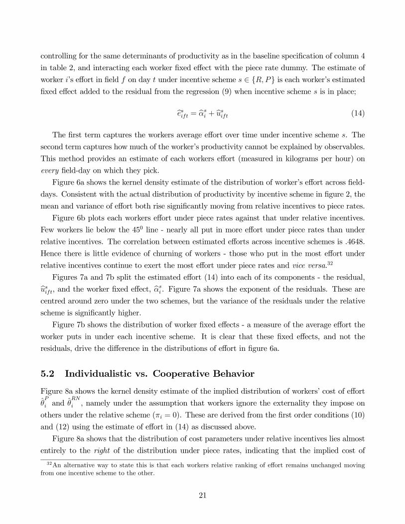
worker i’s effort in field f on day t under incentive scheme s ∈ {R,P} is each worker’s estimatedfixed effect added to the residual from the regression (9) when incentive scheme s is in place;

besift = bαsi + busift (14)

The first term captures the workers average effort over time under incentive scheme s. The

second term captures how much of the worker’s productivity cannot be explained by observables.

This method provides an estimate of each workers effort (measured in kilograms per hour) on

every field-day on which they pick.

Figure 6a shows the kernel density estimate of the distribution of worker’s effort across field-

days. Consistent with the actual distribution of productivity by incentive scheme in figure 2, the

mean and variance of effort both rise significantly moving from relative incentives to piece rates.

Figure 6b plots each workers effort under piece rates against that under relative incentives.

Few workers lie below the 450 line - nearly all put in more effort under piece rates than under

relative incentives. The correlation between estimated efforts across incentive schemes is .4648.

Hence there is little evidence of churning of workers - those who put in the most effort under

relative incentives continue to exert the most effort under piece rates and vice versa.32

Figures 7a and 7b split the estimated effort (14) into each of its components - the residual,busift, and the worker fixed effect, bαsi . Figure 7a shows the exponent of the residuals. These are

centred around zero under the two schemes, but the variance of the residuals under the relative

scheme is significantly higher.

Figure 7b shows the distribution of worker fixed effects - a measure of the average effort the

worker puts in under each incentive scheme. It is clear that these fixed effects, and not the

residuals, drive the difference in the distributions of effort in figure 6a.

5.2 Individualistic vs. Cooperative Behavior

Figure 8a shows the kernel density estimate of the implied distribution of workers’ cost of effort

θ̂P

i and θ̂RN

i , namely under the assumption that workers ignore the externality they impose on

others under the relative scheme (πi = 0). These are derived from the first order conditions (10)

and (12) using the estimate of effort in (14) as discussed above.

Figure 8a shows that the distribution of cost parameters under relative incentives lies almost

entirely to the right of the distribution under piece rates, indicating that the implied cost of

32An alternative way to state this is that each workers relative ranking of effort remains unchanged movingfrom one incentive scheme to the other.

21

effort is higher under relative incentives than under piece rates.

Assuming cost of effort is an innate parameter, the fact that the same distribution of costs

cannot be fitted to both incentive schemes indicates that effort choices are not consistent with

workers ignoring the externality they impose on others under relative incentives.33

Next, we estimate of the distribution of workers’ cost of effort θ̂P

i and θ̂RC

i , namely under the

assumption that workers fully internalize the externality their effort imposes on their co-workers

under the relative incentive scheme.

Following the same methodology as above, we derive the implied distribution of the cost

parameter under each incentive scheme, now assuming that effort levels are chosen according to

(11) and (12).

Figure 8b shows the implied distributions of the cost parameter θi, by incentive scheme. The

distribution of θ̂P

i under piece rates is, by definition, unchanged to that derived above. However,

the distribution of costs under relative incentives θ̂RC

i now lies almost entirely to the left of the

distribution under piece rates.

If workers chose their effort levels cooperatively, then the cost of effort under relative incentives

would have to be significantly lower under relative incentives to fit the observed productivity

data. In other words, productivity is actually too high under relative incentives to be explained

by workers choosing their effort levels cooperatively.

Figures 8a and 8b together reveal an interesting pattern. The observed change in productivity

is too large to be reconciled with the assumption of individualistic behavior but too small to be

reconciled with the assumption of cooperative behavior. This suggests workers behave as if they

internalize the negative externality to some extent. The next subsection explores this idea.

5.3 Social Preferences

We now posit that workers have “social preferences”, namely they place some weight on the

payoffs of their co-workers. We then retrieve the “social weights” (πi) that fit the observed

change in productivity.

To do so, we assume the true cost of effort of each worker is that derived under piece ratesbθPi .34 Given bθPi , we solve the first order conditions of the maximization problem when workers

have social preferences, (2), for each worker’s implied social weight (bπift). We take the median33Evidence of the “ 1N problem”, whereby individuals appear to overestimate the impact of their actions on

their pay has also been found in the literature on team incentives (Hamilton et al (2003)), employee stock optionplans (Jones and Kato (1995)), and firm wide performance bonuses (Knez and Simester (2001)).34Using this measure of ability, we find that groups were equally heterogeneous, in terms of ability, before and

after the change in incentives. Hence there is no evidence of management sorting workers differently by abilityacross the incentive schemes.

22

of these to derive bπi. Note that the social weight is worker specific, namely we assume that eachworker gives the same weight to all co-workers.

The first order condition we calibrate is;

∂yi∂ei

1

(P

i yi)2

"φ0µyiy

¶Xj 6=i

yj − πiXj 6=i

φ0µyjy

¶yj

#=1

NbθPi ei (15)

The resulting distribution of social weights that explains the observed change in productivity

is shown in figure 9. The average worker places a social weight of .65 on the benefits of all others

in the same field-day. Less than 3% of workers have an implied social weight greater than one,

and less than 2% of workers have an implied social weight of less than zero.35

The result indicates that workers behave as if they internalize the externality they impose

on others to a large extent. This is consistent with both collusion and altruism among workers.

Moreover, our setting exhibits features that can facilitate collusion and promote altruism. First,

workers work in close proximity of each other day after day. Second, the workers interact with

each other outside the workplace. Workers live together on the farm and many attend the same

universities in their home countries. The next section explores whether the identity of co-workers

on the field-day explain the workers’ behavior under relative incentives.

6 Incentives, Social Networks and Workers’ Productivity

A natural candidate to explain the extent to which workers place weight on the pay of their

co-workers, and hence internalize the negative externality their effort imposes on others, is the

relationship among workers in any given field-day. To this purpose we use information on the

number of self-reported friends that each worker works alongside on each field-day. Each worker

was asked to name up to five people they were friends with on the farm. A natural hypothesis is

that workers internalize the externality more and hence are less productive when the externality

hurts their friends rather than other workers.36

To investigate this issue table 6 reports estimates of the productivity regression (9) under

relative incentives, where we now additionally control for group composition at the field-day level

as well as the baseline determinants of worker productivity in column 4 of table 2. Note that we

35A negative social weight can be interpreted as the worker being “spiteful” towards others (Levine and Pe-sendorfer (2002)).36Levine and Pesendorfer (2002) show that in an evolutionary equilibrium of a repeated Prisoner’s Dilemma

game in which workers learn which strategies to play, players behave as if they have social preferences. Moreover,the weight each player places on the benefits of another player depends on the relation between players. Theyargue that, “individuals will behave more altruistically when they can identify with the beneficiary of theiraltruism”.

23

identify the effect of group composition on productivity by comparing the productivity of the

same worker, on the same field, working alongside different co-workers on different days when

relative incentives are in place.

Column 1a controls for the share of co-workers in the same field that are friends of worker

i. Having more friends present significantly reduces productivity under relative incentives. The

estimated coefficient implies that if worker i moved from a group with none of her friends to a

group where all five of her friends are present, her productivity would fall by 21%.

In column 1b we interact the share of workers in the same field that are friends of worker i,

with the total number of workers on the field. We find that - (i) having more friends present

significantly reduces productivity under relative incentives; (ii) this effect is smaller the greater

the number of workers in the same field. The latter effect is as expected given that the externality

imposed by i on her friends is smaller when the overall group size is larger.37

Column 1b also shows that the marginal effect of group size is positive and significant, in-

dicating that workers internalize the externality less when they work in larger groups, all else

equal. An increase in group size has two effects on the externality term in the first order condition

under relative incentives, (2). On the one hand, the effect that worker i has on others through

the picking rate, is smaller in larger groups. On the other hand, worker i’s effort affects more

people in larger groups. When workers are of homogeneous ability, the two effects cancel out.

With heterogeneous workers the net effect depends on the ability of the marginal worker relative

to the group.

There is however a third reason why group size may affect productivity. Larger groups may

find it harder to coordinate on the low effort equilibrium. The coefficient on the number of

co-workers in table 6 is consistent with this intuition.

The results in columns 1a and 1b have some obvious alternative interpretations - when workers

work alongside their friends, they exert less effort and become less productive because they talk

and socialize with their friends. Or, alternatively, they may choose to work with their friends

when they feel less prone to work hard.

To shed light on these hypotheses we use the following intuition. Any relationship between

the identity of co-workers and productivity that is unrelated to the incentive scheme in place,

such as socializing with friends, will be present under both incentive schemes. If however the

37The share of friends on the field can also be used to explain the worker’s derived social weights each field-day,bπift. In line with the productivity results, we find that workers place a greater weight on the benefits of co-workerswhen a greater share of co-workers are their friends. The magnitude of the coefficient implies that if worker iwent from having no friends working alongside her, to having only her friends working alongside her, her socialweight would rise by .454. We also find evidence that this effect is larger in smaller groups and that workers’social weights significantly increase as the relative incentive scheme has been in place longer, controlling for theirown work experience. A possible explanation is that later arrivals learn from workers with more experience aboutthe negative externality under the relative incentive scheme.

24

relationship between the identity of co-workers and productivity is related to the externality, it

should affect productivity only under relative incentives.

Columns 2a and 2b then report the same productivity regressions as 1a and 1b when piece

rates are in place. In both cases the share of co-workers that are friends of i has no effect on

productivity under piece rates.38

The finding that the share of friends is a significant negative determinant of productivity

only under relative incentives may still be spurious for the following reason. If workers are more

likely to chat with friends, and work less hard, when they first arrive, the effect of friends on

productivity will only be picked up under the relative incentives scheme, as they were in place for

the first half of the season. Indeed, any factor unrelated to incentives but causing individuals to

treat friends differently over time will be spuriously attributed to the change in incentive scheme.

To check this we examine if under piece rates, the effect of having more friends on the field

is different for those that arrived later and so only worked under piece rates, compared to those

who were also present under the relative incentive scheme. The result in table 7 shows that the

identity of co-workers does not affect productivity under piece rates both for our sample workers

and for workers who arrived to the farm after piece rates were introduced.39

In summary, the evidence indicates that under relative incentives workers internalize the

externality more when they work alongside their friends. The data does not allow us to tell

whether this happens because workers are altruistic towards their friends, or because they fear

punishment and retaliation by their friends. The fact that workers’ productivity is not affected

by the presence of friends under piece rates, however indicates that group composition affects

productivity only when workers’ effort imposes a negative externality on co-workers.40

38Conditional on having at least one friend present, the share of workers that are friends of worker i is onaverage 5% under both schemes. The dispersion is also very similar under the two schemes indicating the resultsunder piece rates are not due to lack of variation in the share of co-workers that are friends.39If workers can devote effort to helping others, they have less incentives to do so under more high powered

incentive schemes (Lazear (1989)). This idea has found empirical support in Drago and Garvey (1998). To checkwhether this explains why friends do not determine productivity under piece rates, we asked workers from whomthey mainly learned to pick (we did not try to elicit workers own evaluations of how much help they offered toothers). Friends however are not an important source of learning in our setting neither for workers who arrivedwhen the relative scheme was in place nor for workers who started under piece rates. For our sample workers,47% said they learned from practice, 26% from workers around them, 19% from supervisors, and 8% from theirfriends. The corresponding figures for those who only worked under piece rates were 43%, 22%, 24% and 4%.40We find similar results using two alternatively defined social networks - the individuals lived with (each worker

shares a caravan with up to 5 other workers), and workers that arrived to the farm together from the same countryon the same day. These results are available from the authors on request.

25

7 Conclusion

This paper uses personnel records to compare workers’ productivity under a relative incentive

scheme to productivity under piece rates. Our estimates indicate that moving from relative

incentives to piece rates causes productivity to rise by at least 50% for the average worker.

We show the difference in productivity is too large to be consistent with workers choosing

effort to maximize their individual net benefits and too small to be consistent with workers

choosing effort levels cooperatively to maximize the sum of all workers’ net benefits. Overall,

workers behave as if they internalize the externality their effort imposes on co-workers to some

extent, especially when a greater share of their co-workers are their close friends.

Throughout we have taken the incentive schemes as given. Our focus has been the response of

workers to an exogenous change in incentives. A separate issue is whether the observed incentive

schemes are optimally designed by the principal. Two questions arise. First, if the relative

incentive scheme was so detrimental to productivity, why was it ever adopted? Second, are piece

rates optimal in this context?

Regarding the use of relative schemes, incentive theory emphasizes that a principal may prefer

relative to absolute performance evaluation when agents face common shocks to productivity. In

line with this, the farm management indeed suggested the relative scheme was mainly adopted

to difference out common shocks which are a key determinant of workers productivity in this

setting.41

The superiority of relative incentives however relies on the assumption that workers play Nash

and maximize their individual rewards - namely they choose effort to maximize their own payoff,

ignoring the externality their effort imposes on others. Under these conditions the marginal

benefit of effort under relative and absolute incentives are approximately equal for large group

sizes. This assumption on worker behavior is not supported in our data. Relative incentives led

to lower productivity because, perhaps surprisingly, workers internalized the negative externality

to some extent.

The finding that workers put a positive weight on their co-workers’ benefit also indicates that

piece rates might not be optimal in this context. Group incentives, namely schemes where the

worker’s pay and her co-workers’ performance are positively related, might elicit more effort at

the same cost to the principal. To explore this issue further, we use our estimates of worker

ability and social weights to simulate effort levels under group incentives.

Under the two incentive schemes we observe in the data, worker i’s compensation is webei,

where w is some constant, e is the average effort of the group, and ei is i’s own effort. Under

41See Lazear and Rosen (1981), Nalebuff and Stiglitz (1983) and Green and Stokey (1983). Relative performanceevaluation may also be preferred to piece rates as it lowers informational rents to high types (Bhaskar (2002)),and reduces incentives of workers to exert effort in influence activity (Milgrom (1988)).

26

relative incentives b = −1 and under piece rates b = 0.We illustrate the effect of group incentiveswithin this class of compensation schemes by setting b > 0. While this need not be the optimal

incentive scheme, it makes the comparison with the observed schemes more transparent.

Figure 10 shows average effort under these three classes of incentive schemes where individual

pay and group performance are negatively correlated (relative incentives), uncorrelated (piece

rates) and positively correlated (group incentives). We derive effort levels under the three al-

ternative assumptions that workers are self interested (π = 0), fully internalize the externality

(π = 1), or have the average social weight derived in section 5 (π = .65). Throughout we adjust

the parameter w to hold the total wage bill constant, and, for simplicity, we assume that workers

are of homogeneous ability.42

The figure shows that the three types of incentive scheme yield the same level of effort only

in the case of pure self interest (π = 0). In line with the previous findings, when workers have

social preferences (π > 0), effort is higher under piece rates than under relative incentives. More

interestingly, the figure also shows that group incentives would, in this context, lead to higher

effort at the same total cost to the principal. The estimates indicate that if π = .65, average

effort would increase by 30% moving from piece rates to a group scheme where individual pay

increases linearly in the average productivity of the group (b = 1).

The intuition for this is that since workers place positive weight on other workers’ pay, the

marginal benefit of effort is higher when effort benefits their co-workers, other things equal.

Importantly, the fact that workers internalize the externality they impose on others provides a

rationale for group incentives even in settings, such as this one, where the production technology

does not exhibit complementarities.43

In summary, the contributions of the paper are twofold. First, we present evidence on the

effect of two types of incentive scheme on the productivity of the same worker. While we analyze

a specific kind of relative scheme, the entire class of relative schemes that rewards individuals

based on their performance relative to their peers’ entail a negative externality similar to the

42We maintain the assumptions that workers’ benefit from pay x is φ (x) = ρx1ρ , and the disutility of effort is

θe2i2 . The θ parameter is set equal to its average estimated value under piece rates and N is set to 40. Worker’scompensation is kept constant at c = 4.5, the average hourly pay. The Nash equilibrium effort level as a functionof b then is;

e =

Ãc1/ρ(1 + b 1N + πbN−1N )

θ

!1/2Note the effect of b - the relationship between individual pay and group performance - on effort depends on the

sign and the magnitude of the social weight π.43Rotemberg (1994)’s model shows that group incentives are optimal if workers are altruistic. This is consistent

with Roethlisberger and Dickson (1939)’s results from the Hawthorne experiments where productivity increasedsignificantly for workers that were given group incentives and were allowed to socialize. Sen (1966) analyzes theallocation rule that leads to Pareto efficiency in a cooperative whose workers place a positive weight on eachother’s material benefits. He shows the optimal rule is a combination of individual and group rewards.

27

one analyzed here. The finding that workers internalize the externality to some extent has impli-

cations for the design of relative incentive schemes in general. In addition, our findings suggest

that there ought to be productivity gains if workers’ compensations were positively correlated to

the performance of their co-workers.

Second, we provide evidence on how workers behave in a real world situation where individual

and social optima do not coincide. In doing so, we integrate recent insights from the experimental

literature on social preferences with the literature on the provision of incentives.

In general, our analysis illustrates that understanding worker preferences is key for the optimal

choice between alternative incentive schemes. In particular, to the extent that workers place some

weight, either positively or negatively, on the effect of their actions on the other workers’ pay,

group or relative incentive schemes can outperform piece rates in terms of productivity.

The findings thus provide insights for further developments of incentive theory and shed new

light on and old idea - the interplay between social effects and the provision of incentives within

firms.44

8 Appendix: Quality and Quantity

The evidence presented earlier suggested that the operation of the farm did not change along

a number of important margins over the season - the stock of workers available, the length of

the working day, and the allocation of supervisors. However one margin that may have been

unintentionally affected by the change in incentives is the quality of picking.

Pickers are expected to classify fruit as either class one - suitable as supermarket produce, or

class two - suitable as market produce. This classification takes place within the field by each

worker as they pick. Each class of fruit is then placed into a separate container. After fruit has

been picked it is transported to a cooled warehouse for packing. In the packhouse each container

passes through a quality check. Whenever a class two fruit is detected in a class one container,

it is removed - downgraded - and transferred to a class two container. By the time the fruit

picked from a given field-day arrives in the farm packhouse for inspection, misclassifications of

fruit cannot be traced back to individual workers.

The electronic system used to record individual productivity data is not the same as that

which records misclassifications of fruit at the field-day level in the packhouse. It is thus not

possible to match every field-day from the productivity and packhouse databases. However we

44The idea that human relations affect workplace performance goes back to Mayo (1933), Barnard (1938),Roethlisberger and Dickson (1939), and Roy (1952). More recently, Kandel and Lazear (1992), Lazear (1989),Rotemberg (1994) and Fershtman et al (2003) have developed models incorporating social concerns into theanalysis of behavior within firms.

28

are able to do this for a subsample of 67 field-days. In this sample, 30 field-days were operated

under relative incentives, 37 were operated under piece rates.45

In table A1 we assess whether the trade-off between the quality and quantity of picking

changed significantly with the change in incentive scheme. The measure of the quality of picking

is the log of the ratio of the total fruit of class two that is misclassified as class one, to the

total fruit picked classified as class two. On average under relative incentives, 15% of fruit is

misclassified as class one. Under piece rates this falls to 12%, although this difference is not

significant.

In column 1 we regress this measure of the quality of picking on a dummy for the introduction

of the piece rate and field fixed effects. The incentive scheme in place has no affect on the quality

of picking. Column 2 shows this to be the case when the tons of class two fruit picked is controlled

for. In column 3 we additionally control for a time trend and its square. We find that the level

of misclassification of fruit picked increases over time, but at a decreasing rate.

Finally, column 4 additionally controls for the field life cycle, and meteorological factors.

Again the quality of picking does not respond to the change in incentives, all else equal.

The productivity gains achieved under piece rates were not at the expense of a lower quality

of picking. Combined with the fact that worker pay remained constant over the season, the

change in incentives unambiguously led farm management to become better off.

References

[1] baker.g (1992) “Incentive Contracts and Performance Measurement”, Journal of Political

Economy 100: 598-614.

[2] barnard.c (1938) The Functions of the Executive, Cambridge: Harvard University Press.

[3] becker.b and m.huselid (1992) “The Incentive Effects of Tournament Compensation

Systems”, Administrative Science Quarterly 37: 336-50.

[4] bhaskar.v (2002) Relative Performance Evaluation and Limited Liability, mimeo Univer-

sity of Essex.

[5] bull.c, a.schotter and k.weigelt (1987) “Tournaments and Piece Rates: An Experi-

mental Study”, Journal of Political Economy 95: 1-33.

45This partly includes the two main fields in our sample that are operated on for the most days under eachincentive scheme. The productivity and packhouse data are merged assuming that fruit is stored in the packhousefor two days after it is picked. We were informed by farm management this was the modal time between pickingand packing.

29

[6] camerer.c, l.babcock, g.loewenstein and r.thaler (1997) “Labor Supply of New

York City Cabdrivers: One Day At A Time”, Quarterly Journal of Economics 112: 407-41.

[7] drago.r and g.t.garvey (1998) “Incentives for Helping on the Job: Theory and Evi-

dence”, Journal of Labor Economics 16: 1-25.

[8] ehrenberg.r and m.bognanno (1990) “The Incentive Effects of Tournaments Revisited:

Evidence from the European PGA Tour”, Industrial Labor Relations Review 43: 74-89.

[9] fehr.e and u.fischbacher (2002) “Why Social Preferences Matter - The Impact of Non-

Selfish Motives on Competition, Cooperation and Incentives”, Economic Journal 112: C1-

C33.

[10] fehr.e and s.gachter (2000) “Cooperation and Punishment in Public Goods Experi-

ments”, American Economic Review 90: 980-94.

[11] fehr.e and k.m.schmidt (1999) “A Theory of Fairness, Competition and Cooperation”,

Quarterly Journal of Economics 114: 817-68.

[12] fershtman.c, h.k.hvide and y.weiss (2003) Cultural Diversity, Status Concerns and

the Organization of Work, CEPR Discussion Paper No.3982.

[13] foster.a.d and m.r.rosenzweig (1994) “A Test for Moral Hazard in the Labor Market:

Effort, Health and Calorie Consumption”, Review of Economics and Statistics 76: 213-27.

[14] green.j.r and n.l.stokey (1983) “A Comparison of Tournaments and Contracts”, Jour-

nal of Political Economy 91: 349-64.

[15] hamilton.b.h, j.a.nickerson and h.owan (2003) “Team Incentives and Worker Hetero-

geneity: An Empirical Analysis of the Impact of Teams on Productivity and Participation”,

forthcoming Journal of Political Economy.

[16] holmstrom.b and p.milgrom (1991) “Multitask Principal-Agent Analyses: Incentive

Contracts, Asset Ownership, and Job Design”, Journal of Law, Economics and Organization

7:24-52.

[17] jones.d and t.kato (1995) “The Productivity Effects of Employee Stock-Ownership Plans

and Bonuses: Evidence from Japanese Panel Data”, American Economic Review 85: 391-

414.

[18] kandel.e and e.lazear (1992) “Peer Pressure and Partnerships”, Journal of Political

Economy 100: 801-13.

30

[19] knez.m and d.simester (2001) “Firm-Wide Incentives and Mutual Monitoring at Conti-

nental Airlines”, Journal of Labor Economics 19: 743-72.

[20] knoeber.c and w.thurman (1994) “Testing the Theory of Tournaments: An Empirical

Analysis of Broiler Production”, Journal of Labor Economics 12: 155-79.

[21] laffont.j.j and matoussi.m (1995) “Moral Hazard, Financial Constraints and Share-

cropping in El Oulja”, The Review of Economic Studies 62: 381-99.

[22] lazear.e.p (1989) “Pay Equality and Industrial Politics”, Journal of Political Economy

87: 1261-84.

[23] lazear.e.p (2000) “Performance Pay and Productivity”, American Economic Review 90:

1346-61.

[24] lazear.e.p and s.rosen (1989) “Rank Order Tournaments as OptimumLabor Contracts”,

Journal of Political Economy 89: 841-64.

[25] ledyard.j. (1995) “Public Goods: A Survey of Experimental Research” in Kagel.J, Roth.

A (eds.), The Handbook of Experimental Economics, Princeton: Princeton University Press,

111-94.

[26] levine.d.k and w.pesendorfer (2002) The Evolution of Cooperation Through Imitation,

mimeo UCLA.

[27] masclet.d, c.noussair, s.tucker and m.c.villeval (2003) “Monetary and Nonmone-

tary Punishment in the Voluntary Contributions Mechanism”, American Economic Review

93: 366-80.

[28] mayo.e (1933) The Human Problems of an Industrial Civilization, New York: Macmillan.

[29] milgrom.p.r (1988) “Employment Contracts, Influence Activities, and Efficient Organiza-

tion Design”, Journal of Political Economy 96: 42-60.

[30] nalebuff.b.j and j.e.stiglitz (1983) “Prizes and Incentives: Toward a General Theory

of Compensation and Competition”, Bell Journal of Economics 14: 21-43.

[31] oettinger.g.s (1999) “An Empirical Analysis of the Daily Labor Supply of Stadium Ven-

dors”, Journal of Political Economy 107: 360-92.

[32] paarsch.h.j and b.s.shearer (1996) Fixed Wages, Piece Rates, and Intertemporal Pro-

ductivity: A Study of Tree Planters in British Columbia, mimeo Université Laval.

31

[33] prendergast.c (1999) “The Provision of Incentives in Firms”, Journal of Economic Lit-

erature 37: 7-63.

[34] roethlisberger.f.j and w.dickson (1939) Management and the Worker, Cambridge:

Harvard University Press.

[35] rotemberg.j.j (1994) “Human Relations in the Workplace”, Journal of Political Economy

102: 684-717.

[36] roy.d (1952) “Quota Restriction and Goldbricking in a Machine Shop”, American Journal

of Sociology 57: 427-42.

[37] sen.a.k (1966) “Labour Allocation in a Cooperative Enterprise”, The Review of Economic

Studies 33: 361-71.

[38] sethi.r and e.somanathan (1999) Preference Evolution and Reciprocity, mimeo Univer-

sity of Michigan.

[39] shearer.b.s (2004) “Piece Rates, Fixed Wages and Incentives: Evidence From a Field

Experiment”, Review of Economic Studies 71: 513-34.

[40] silverman.b.w (1986)Density Estimation for Statistics and Data Analysis, London: Chap-

man and Hall.

32

Figure 1: Productivity (kilogram/hour) Over the Season

Figure 2: Distribution of Productivity (kg/hr) by Incentive Scheme

Pro

duct

ivity

(kilo

gram

/hou

r)

First field Second field

31may2002 30jun2002 31jul2002 31aug2002

2

4

6

8

10

12

14

Introduction of Piece Rates

Prod

uctiv

ity (k

ilogr

am/h

our)

Notes: In figure 1, average productivity on the two main fields is shown for those workers that work at least 10 field-days under each incentive scheme. These fields are operated for the greatest number of days under each incentive scheme. Together they contribute one third of the total worker-field-day observations. The kernel density estimates in figure 2, and all those that follow, are calculated using an Epanechnikov kernel, based on 50 grid points and the bandwidth suggested by Silverman (1986, pp38-40).

First Field Second Field

May 31st June 30th July 31st Aug 31st

Productivity Under Piece Rate Productivity Under Average Syst

0 4 8 12 16 20

0

.02

.04

.06

.08

.1

.12

.14

.16

Productivity Under Piece Rate

Productivity Under Relative Incentives

Freq

uenc

y D

ensi

ty

Productivity (kilogram/hour)

Figure 3: Cumulative Distribution of Arrival and Departure of Workers

(mean) lastday

(mean) cum_first (mean) cum_last

05apr2002 30apr2002 31may2002 30jun2002 31jul2002 31aug200230sep2002

0

.1

.2

.3

.4

.5

.6

.7

.8

.9

1

Introduction of Piece Rates

Cum

ulat

ive

Freq

uenc

y

Arrivals

April 30th May 31st June 30th July 31st Aug 31st Sept 30th April 5th

Departures

Notes: The sample for this figure includes all workers on the farm that are available for picking.

Figure 4a: Aggregate Kilos Picked Per Day Over the Season

Figure 4b: Aggregate Hours Worked Per Day Over the Season

Figure 4c: Total Number of Pickers Over the Season

Num

ber o

f Pic

kers

31may2002 30jun2002 31jul2002 31aug2002

-100

-75

-50

-25

0

25

50

75

100

Man

Hou

rs W

orke

d

31may2002 30jun2002 31jul2002 31aug2002

-100

-75

-50

-25

0

25

50

75

100

Kilo

gram

s P

icke

d

31may2002 30jun2002 31jul2002 31aug2002

-100

-75

-50

-25

0

25

50

75

100

Notes: The sample in each series is based on all workers that are present on the farm on any given day.

Agg

rega

te K

ilos

Pick

ed p

er D

ay,

perc

enta

ge d

evia

tion

from

mea

n

Introduction of Piece Rates

Introduction of Piece Rates

May 31st June 30th July 31st Aug 31st

May 31st June 30th July 31st Aug 31st

Introduction of Piece Rates

May 31st June 30th July 31st Aug 31st

Agg

rega

te N

umbe

r of P

icke

rs p

er D

ay,

perc

enta

ge d

evia

tion

from

mea

nA

ggre

gate

Hou

rs W

orke

d pe

r Day

,pe

rcen

tage

dev

iatio

n fr

om m

ean

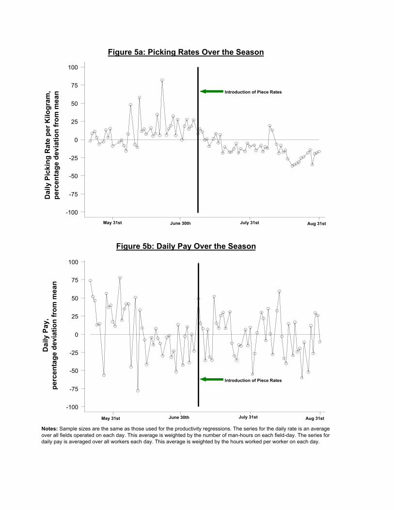
Figure 5a: Picking Rates Over the Season

Figure 5b: Daily Pay Over the Season

Pay

from

Pic

king

31may2002 30jun2002 31jul2002 31aug2002

-100

-75

-50

-25

0

25

50

75

100

Piec

e R

ate

31may2002 30jun2002 31jul2002 31aug2002

-100

-75

-50

-25

0

25

50

75

100

Notes: Sample sizes are the same as those used for the productivity regressions. The series for the daily rate is an average over all fields operated on each day. This average is weighted by the number of man-hours on each field-day. The series for daily pay is averaged over all workers each day. This average is weighted by the hours worked per worker on each day.

Dai

ly P

icki

ng R

ate

per K

ilogr

am,

perc

enta

ge d

evia

tion

from

mea

n D

aily

Pay

,pe

rcen

tage

dev

iatio

n fr

om m

ean

Introduction of Piece Rates

Introduction of Piece Rates

May 31st June 30th July 31st Aug 31st

May 31st June 30th July 31st Aug 31st

Figure 6a: Kernel Density Estimates of Effort by Incentive Scheme

Figure 6b: Scatter Plot of Efforts in the Two Incentive Schemes

ax

density: (mean) aveeffort_p density: (mean) aveeffort_a

0 1 2 3 4 5 6

0

.5

1

Freq

uenc

y D

ensi

ty

Estimated Effort (kg per hour)

Estimated Effort UnderPiece Rate

Estimated Effort Under Relative Incentives

The total cost of effort is assumed to be quadratic in effort.

(mean) aveeffort_a

(mean) aveeffort_p fortyfive

1 2 3 4

1

2

3

4

5

6

Effort Under Relative Incentives (kg per hour)

Effo

rt U

nder

Pie

ce R

ate

(kg

per h

our)

45° line

Notes: Kernel density estimates are calculated using an Epanechnikov kernel. The underlying benefit function used to estimate worker effort is assumed to be;

21

2)( xx =ϕ

Figure 7a: Residuals by Incentive Scheme

Figure 7b: Kernel Density Estimates of Fixed Effectsby Incentive Scheme

lresA

density: lresA density: lresP

-2 -1 0 1 2

0

.5

1

Freq

uenc

y D

ensi

ty

Residuals UnderPiece Rate

Residuals UnderRelative Incentives

Notes: Both figures are for the 142 workers in the productivity regressions. The residuals for each worker-field-day observation are derived from estimating the baseline productivity specification, in column 4 of table 3. The kernel density estimates are calculated using an Epanechnikov kernel. A Kolmogorov-Smirnov equality of distributions test rejects the null against a one-sided alternative that the fixed effects under relative incentives are lower than under the piece rate (p-value .000.).

ax

density: (mean) aveFE_p density: (mean) aveFE_a

0 1 2 3 4 5 6

0

.5

1

Fixed Effects Under Piece Rate

Fixed Effects Under Relative Incentives

Freq

uenc

y D

ensi

ty

Fixed Effect )ˆ( siα

Residual ))ˆ(exp( siftu

Figure 8a: Kernel Density Estimates of Cost of Effort Parameter, by Incentive Scheme Assuming Individualistic Behavior

Figure 8b: Kernel Density Estimates of Cost of Effort Parameter, by Incentive Scheme Assuming Cooperative Behavior

ax

density: (mean) medtheta_su2 density: (mean) medtheta_pu2

0 .5 1

0

2

4

6

axis1

density: (mean) medtheta_pu2 density: (mean) medtheta_au2

0 .5 1 1.5 2 2.5

0

1

2

3

Cost of Effort Parameter (θ)Under Piece Rate

Cost of Effort Parameter (θ)Under Relative Incentives

Cost of Effort Parameter (θ)

Freq

uenc

y D

ensi

tyFr

eque

ncy

Den

sity

Cost of Effort Parameter (θ) Under Piece Rate

Cost of Effort Parameter (θ) Under Relative Incentives

Notes: Kernel density estimates are calculated using an Epanechnikov kernel. The underlying benefit function is assumed to be;

The total cost of effort is assumed to be quadratic in effort. Under individualistic behavior we imply the worker chooses their effort to maximize their own net benefits. Under cooperative behavior we imply the worker chooses their effort level to maximize the sum of all workers utilities.

Cost of Effort Parameter (θ)

21

2)( xx =ϕ

Figure 9: Kernel Density Estimates of Social Weight (π)de

nsity

: (m

ean)

med

alph

au2

(mean) medalphau2-.5 0 .5 1

0

.5

1

1.5

2

Social Weight (π)

Freq

uenc

y D

ensi

ty

Notes: Kernel density estimates are calculated using an Epanechnikov kernel. The underlying benefit function is assumed to be;

The total cost of effort is assumed to be quadratic in effort.

21

2)( xx =ϕ

Relative incentives: b=-1 Piece rates: b=0 Group incentives: b=1

Effort, calibratedEffort, estimated from productivity data

3.68

Estimated Effort Under the Three Incentive Schemes When π=.65

1.661.67

2.822.86

21.510.50-0.5-1

5

3.75

2.5

1.25

0

x

y

x

y

π=0

π=.65

π=1

Group pay: b>0

b

Notes: The figure shows the Nash equilibrium efforts for π=0,.65, and 1, as a function of the parameter b in the pay schedule;

Throughout, the parameter w is adjusted to hold constant the total wage bill, and N=40. We assume workers have the same social weight (either 0,.65 or 1), and are of homogeneous ability. The θ parameter is set equal to its average estimated value under piece rates. Worker's benefit from pay x is assumed to be;

The relative incentive scheme observed in the data corresponds to b=-1. Piece rates correspond to b=0. Group pay corresponds to b>0.

2/12)( xx =ϕ

Piece rates: b=0Relative incentives: b=-1

Effort

Figure 10: Incentive Schemes and Effort, Holding Total Wage Bill Constant

ib eewpay =

Table 1: Unconditional Differences in Productivity and other Farm Variables.

Mean, standard errors in parentheses, and confidence interval in brackets

Relative Incentives Piece Rates Difference

Worker Productivity 5.01 7.98(.243) (.208)

[ 4.53, 5.49 ] [ 7.57, 8.39 ]

Kilos Picked Per Day 23.2***

Hours Worked Per Day -.475

Group Size 41.1 38.1(2.38) (1.29)

Daily Pay 1.80

Rate per Kilogram Picked -.105***Confidential

-3.11

2.97***

Confidential

Confidential

Confidential

Notes : *** denotes significance at 1%. Sample sizes are the same as those used for the productivity regressions. Standard errors and confidence intervals take account of the observations being clustered by field-day. Daily pay refers to pay from picking only. Some information in the table is not shown due to confidentiality requirements.

Table 2: The Effect of Piece Rates on Productivity

Dependent Variable = Log of worker's productivity (kilogram picked per hour per field-day)Robust standard errors reported in parentheses, allowing for clustering at field-day level

(1) Unconditional (2) Worker Heterogeneity

(3) Field Heterogeneity (4) Controls

Piece rate .530*** .515*** .460*** .577***(.059) (.056) (.070) (.098)

Time trend .004(.003)

Field life cycle -1.16***(.362)

Worker experience .077***(.031)

Worker fixed effects No Yes Yes Yes

Field fixed effects No No Yes Yes

Adjusted R-squared .1607 .2925 .3407 .3640

Number of observations (worker-field-day) 10215 102151021510215

Notes: *** denotes significance at 1%, ** at 5%, and * at 10%. Standard errors are clustered at the field-day level. All continuous variables are in logs. The sample is restricted to workers who have worked at least 10 days under both incentive schemes. There are 142 workers, 22 fields and 108 days in the sample.

Table 3: Econometric Concerns - Spurious Time Effects

Dependent Variable = Log of worker's productivity (kilogram picked per hour per field-day)Robust standard errors reported in parentheses, allowing for clustering at field-day level

(1) Main Fields (2) Twenty Days (3) Fake Piece Rate: Fields

(4) Fake Piece Rate: Workers

Piece rate .610*** .387***

(.070) (.110)

.156

(.196)

-.009

(.091)

Worker fixed effects Yes Yes Yes Yes

Field fixed effects Yes Yes Yes Yes

Other Controls No No Yes Yes

Adjusted R-squared .4032 .2922 .4927 .5921

Fake piece rate based on field life cycle

Fake piece rate based on number of days present on the farm

2863 879Number of observations (worker-field-day) 29693404

Notes: *** denotes significance at 1%, ** at 5%, and * at 10%. Robust standard errors are calculated throughout, allowing for clustering at the field-day level in all columns. All continuous variables are in logs. The sample is restricted to workers who have worked at least 10 days under both incentive schemes. The sample in column 1 is restricted to workers that have only been picking on that day. The sample in column 2 is restricted to the two main fields operated on over the season. The sample in column 3 is restricted to 10 days either side of the change in incentive schemes. Other controls include worker picking experience, field life cycle, and a linear time trend.

Table 4: Econometric Concerns - Task Allocation and Sample Selection

Dependent Variable = Log of worker's productivity (kilogram picked per hour per field-day)Robust standard errors reported in parentheses, allowing for clustering at field-day level

(1) Only Picking Tasks

(2) "Reallocated Workers" Sample

(3) Group Composition

Piece rate .644*** .625*** .572***(.113) (.148) (.118)

-.006(.067).018

(.068)

Worker fixed effects Yes Yes YesField fixed effects Yes Yes YesOther Controls Yes Yes YesAdjusted R-squared .3704 .2869 .3639

102151286

Number of "Reallocated Workers" on field-day

Total number of workers on field-day

Number of observations (worker-field-day) 7077

Notes: *** denotes significance at 1%, ** at 5%, and * at 10%. Robust standard errors are calculated throughout, allowing for clustering at the field-day level in all columns. All continuous variables are in logs. The sample in columns (1) and (3) is restricted to workers who have worked at least 10 days under both incentive schemes. The sample in column 1 is further restricted to workers that have only been picking on that day. The sample in column (2) is restricted to workers who have worked at least 10 days under the relative incentive schemes and less than 10 days under piece rates. Other controls include worker picking experience, field life cycle, and a linear time trend.

Table 5: Econometric Concerns - Endogenous Responses

Dependent Variable = Log of worker's productivity (kilogram picked per hour per field-day)Robust standard errors reported in parentheses, allowing for clustering at field-day level

(1) Anticipation(2) Drop Last 10 Days

Under Relative Incentives

(3) Drop First 10 Days Under Piece Rate (4) Tenure (5) Entrenchment

Piece rate .456*** .753*** .719*** .629*** .630***

(.125) (.138) (.114) (.098) (.098)

-.166

(.124)

.027*** .029***

(.005) (.005)

.115***

(.052)

-.140

(1.20)

Worker fixed effects Yes Yes Yes Yes Yes

Field fixed effects Yes Yes Yes Yes Yes

Other Controls Yes Yes Yes Yes Yes

Adjusted R-squared .3665 .3813 .4245 .3950 .3956

8873 10215 1021510215 9340

Dummy equal to one for the week prior to the introduction of the piece rate

Number of observations (worker-field-day)

Tenure under piece rates

Piece rate x [experience under relative scheme - mean experience under relative scheme]Tenure x [experience under relative scheme - mean experience under relative scheme] x 10-3

Notes: *** denotes significance at 1%, ** at 5%, and * at 10%. Robust standard errors are calculated throughout, allowing for clustering at the field-day level in all columns. All continuous variables are inlogs. The sample is restricted to workers who have worked at least 10 days under both incentive schemes. The tenure variable controls for the number of days piece rates have been in place for. Other controls include worker picking experience, field life cycle, and a linear time trend.

Table 6: The Effect of Group Composition on Productivity by Incentive Scheme

Dependent Variable = Log of worker's productivity (kilogram picked per hour per field-day)Robust standard errors reported in parentheses, allowing for clustering at field-day level

Share of workers in the field that are friends -1.68*** -5.52** .072 1.17(.647) (2.36) (.493) (1.60)

1.60** -.285(.684) (.501)

Number of workers in same field .182 .085(.117) (.069)

Marginal Effect of Group Size (at mean friends share) .236** .076(.110) (.065)

Worker fixed effects Yes Yes Yes YesField fixed effects Yes Yes Yes YesOther Controls Yes Yes Yes YesAdjusted R-squared .3470 .3620 .3065 .3081

4400

(2b) Piece Rates

44002860

(1a) Relative Incentives

(2a) Piece Rates

(1b) Relative Incentives

2860

Share of workers in the field that are friends x number of workers in same field

Number of observations (worker-field-day)

Notes: *** denotes significance at 1%, ** at 5%, and * at 10%. Robust standard errors are calculated throughout, allowing for clustering at the field-day level. All continuous variables are in logs. The sample is restricted to workers who have worked at least 10 field-days under both incentive schemes. Other controls include worker experience, field life cycle, and a linear time trend.

Table 7: Robustness Checks on The Effects of Group Composition on Productivity by Incentive Scheme

Dependent Variable = Log of worker's productivity (kilogram picked per hour per field-day)Robust standard errors reported in parentheses, allowing for clustering at field-day level

(1) (2)

Share of workers in the field that are friends .200 1.13(.495) (1.57)

-.227(.498)

Number of workers in same field .073(.069)

-2.65 5.93(1.90) (7.00)

-3.70(2.53).110

(.230)

Worker fixed effects Yes YesField fixed effects Yes YesOther Controls Yes YesAdjusted R-squared .3619 .3636

Piece Rates

Number of workers in same field x worked only under piece rates

Number of observations (worker-field-day) 4667

Share of workers in the field that are friends x number of workers in same field

Share of workers in the field that are friends x number of workers in same field x worked only under piece rates

Share of workers in the field that are friends x worked only under piece rates

Piece Rates

4667

Notes: *** denotes significance at 1%, ** at 5%, and * at 10%. Robust standard errors are calculated throughout, allowing for clustering at the field-day level. All continuous variables are in logs. Other controls include worker experience, field life cycle, and a linear time trend. The sample also includes workers that have only picked under piece rates.

Table A1: The Effect of Piece Rates on the Quality of Picking

Dependent Variable = Log of total fruit of class two misclassified as class one, at the packfield-day levelRobust standard errors reported in parentheses

(1) (2) (3) (4)

Piece rate .330 .336 .434 .399(.257) (.265) (.322) (.304)

Tons of class two fruit picked x 10-3 -.794 -.401 -.249(.845) (.780) (.859)

Time trend .067** .060*(.032) (.033)

Time trend squared x 10-3 -.349** -.330**(.146) (.151)

Field life cycle -.520(.666)

Minimum temperature .059(.039)

Maximum temperature .028(.043)

Hours of sunshine -.009(.035)

Packfield fixed effects Yes Yes Yes Yes

R-squared .0724 .0901 .1845 .2224

67Number of observations (field-day) 67 67 67

Notes: *** denotes significance at 1%, ** at 5%, and * at 10%. Robust standard errors are calculated throughout. Data is based on the packhouse software system. It is assumed that all fruit arrives in the packhouse two days after it is picked. Variables are only available aggregated on field-day level where fields are further grouped according to fruit variety. This forms a packfield. The sample is restricted to those packfields that operated under both incentive schemes. All right hand side variables are lagged by two days to allow for a time lag between picking and packing. Temperature variables correspond to a 0900-0900 time frame. Hours of sunshine are measured daily.