Embed Size (px)
Citation preview
IZA DP No. 2840
Relative Income, Happiness and Utility:An Explanation for the Easterlin Paradoxand Other Puzzles
Andrew E. ClarkPaul FrijtersMichael Shields
DI
SC
US
SI
ON
PA
PE
R S
ER
IE
S
Forschungsinstitutzur Zukunft der ArbeitInstitute for the Studyof Labor
June 2007
Relative Income, Happiness and Utility:
An Explanation for the Easterlin Paradox and Other Puzzles
Andrew E. Clark Paris School of Economics and IZA
Paul Frijters
Queensland University of Technology
Michael Shields University of Melbourne and IZA
Discussion Paper No. 2840 June 2007
IZA
P.O. Box 7240 53072 Bonn
Germany
Phone: +49-228-3894-0 Fax: +49-228-3894-180
E-mail: [email protected]
Any opinions expressed here are those of the author(s) and not those of the institute. Research disseminated by IZA may include views on policy, but the institute itself takes no institutional policy positions. The Institute for the Study of Labor (IZA) in Bonn is a local and virtual international research center and a place of communication between science, politics and business. IZA is an independent nonprofit company supported by Deutsche Post World Net. The center is associated with the University of Bonn and offers a stimulating research environment through its research networks, research support, and visitors and doctoral programs. IZA engages in (i) original and internationally competitive research in all fields of labor economics, (ii) development of policy concepts, and (iii) dissemination of research results and concepts to the interested public. IZA Discussion Papers often represent preliminary work and are circulated to encourage discussion. Citation of such a paper should account for its provisional character. A revised version may be available directly from the author.
IZA Discussion Paper No. 2840 June 2007
ABSTRACT
Relative Income, Happiness and Utility: An Explanation for the Easterlin Paradox and Other Puzzles
The well-known Easterlin paradox points out that average happiness has remained constant over time despite sharp rises in GNP per head. At the same time, a micro literature has typically found positive correlations between individual income and individual measures of subjective well-being. This paper suggests that these two findings are consistent with the presence of relative income terms in the utility function. Income may be evaluated relative to others (social comparison) or to oneself in the past (habituation). We review the evidence on relative income from the subjective well-being literature. We also discuss the relation (or not) between happiness and utility and discuss some non-happiness research (behavioural, experimental, neurological) dealing with income comparisons. We last consider how relative income in the utility function affects economic models of behaviour in a number of different domains. JEL Classification: D01, D31, H00, I31, J28 Keywords: income, happiness, utility, comparison, habituation Corresponding author: Andrew E. Clark PSE 48 Boulevard Jourdan 75014 Paris France E-mail: [email protected]
Relative Income, Happiness and Utility:
An Explanation for the Easterlin Paradox and Other Puzzles
ANDREW E. CLARK, PAUL FRIJTERS and MICHAEL A. SHIELDS1
June 2007
“Every pitifulest whipster that walks within a skin has had his head filled with the notion that he
is, shall be, or by all human and divine laws ought to be, ‘happy’” (Thomas Carlyle).
1. Income, Happiness and the Easterlin Paradox
Studying the causes and correlates of human happiness has become one of the hot topics in
economics over the last decade, with both the size and depth of the literature increasing at an
exponential rate (Kahneman and Krueger, 2006). One of the main catalysts in the literature on
income and happiness has been Easterlin’s seminal article (1974; updated in 1995), setting out
the ‘paradox’ of substantial real income growth in Western countries over the last fifty years, but
without any corresponding rise in reported happiness levels. Similar studies have also since been
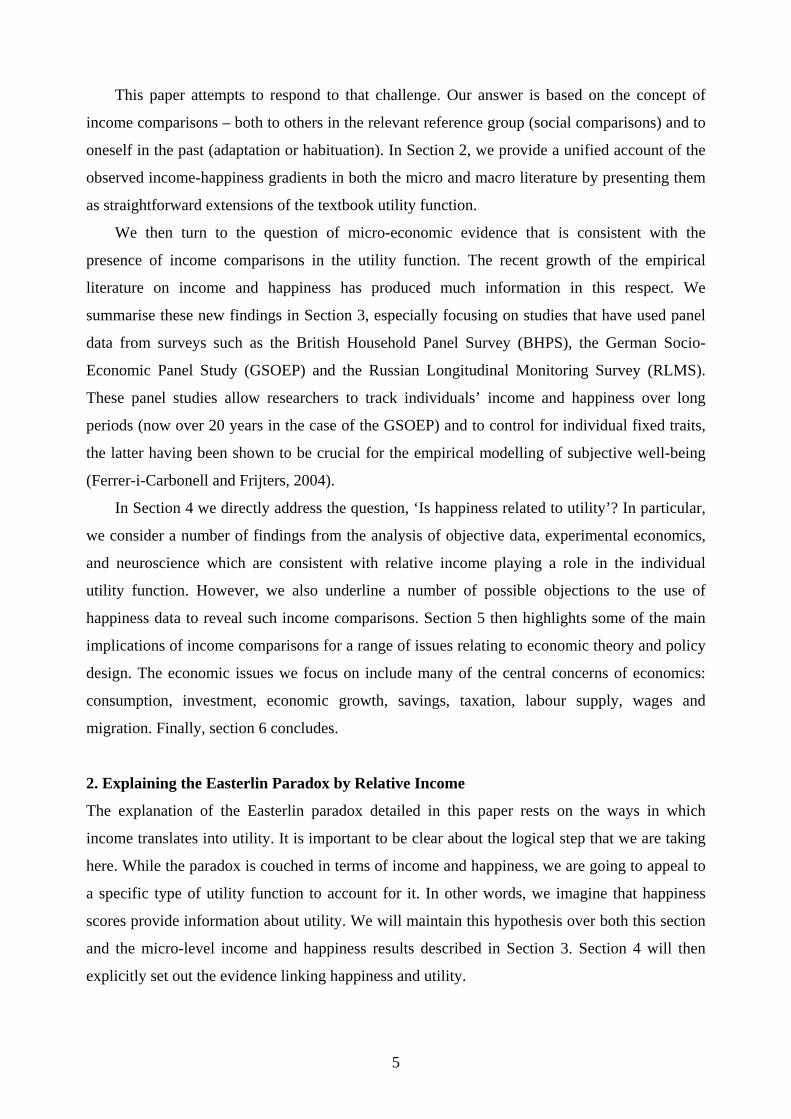
conducted by psychologists (Diener et al., 1995) and political scientists (Inglehart, 1990). Figure
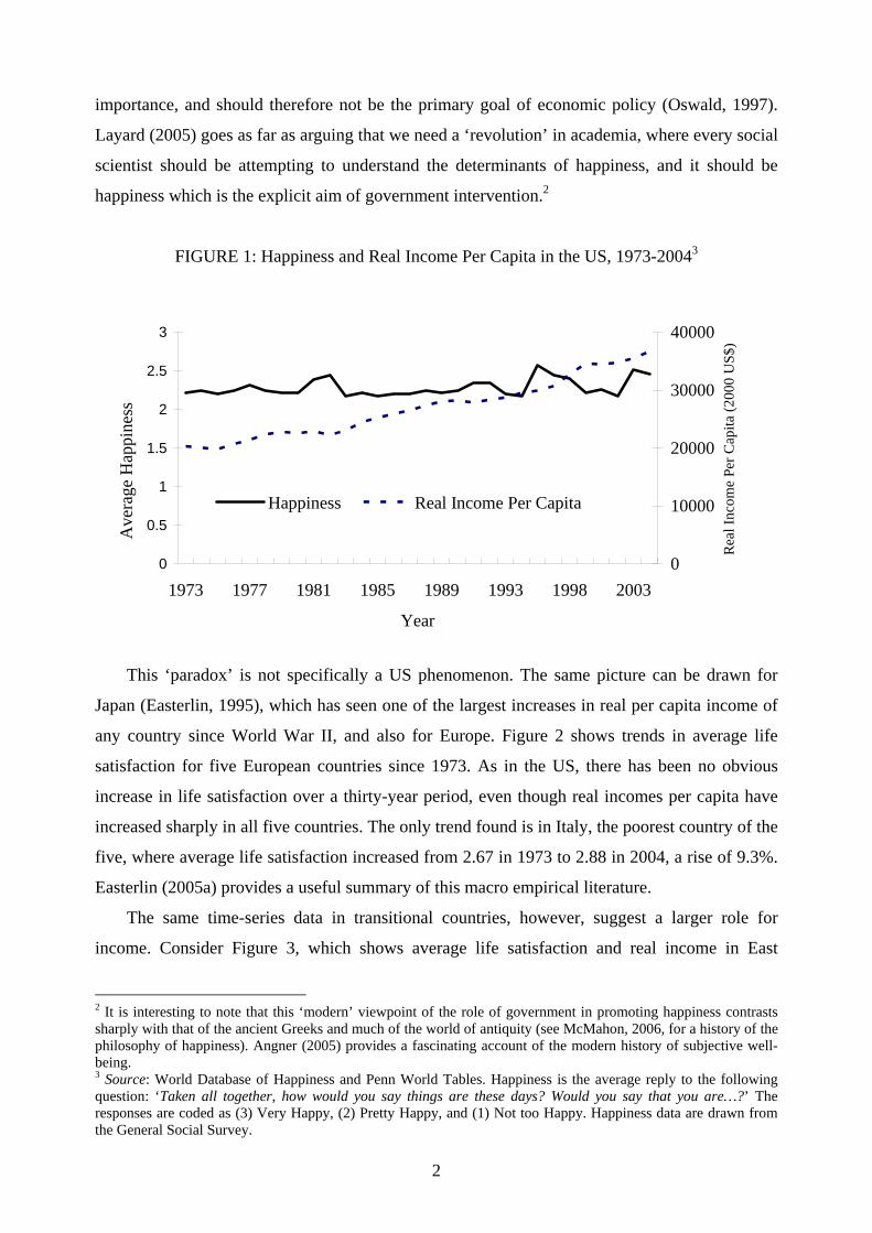
1 shows an Easterlin graph for the US over the period 1973-2004. While real income per capita
almost doubles, happiness (from the General Social Survey) shows essentially no trend. From
this figure, to borrow a term from health economics, it looks as if individuals in the US are ‘flat
of the curve’, with additional income buying little if any extra happiness. It has been argued that
once an individual rises above a poverty line or ‘subsistence level’, the main source of increased
well-being is not income but rather friends and a good family life (see, for example, Lane,
2001). This ‘subsistence level’ could be as low as US$10,000 per annum (as reported in Frey
and Stutzer, 2002a; and McMahon, 2006). Following on with this argument, the radical
implication for developed countries at least is that economic growth per se is of little
1 Clark: Paris School of Economics, France, and IZA, Germany; Frijters: School of Economics and Finance, Queensland University of Technology, Australia; Shields: Department of Economics, University of Melbourne, Australia. We are grateful to the editor and two anonymous referees for very constructive comments. We also thank Colin Camerer, Richie Davidson, Ed Diener, Dick Easterlin, Ada Ferrer-i-Carbonell, Carol Graham, John Helliwell, Felicia Huppert, Danny Kahneman, Brian Knutson, George Loewenstein, Sonja Lyubomirsky, Dan Mroczek, Yew-Kwang Ng, Matthew Rablen, Larry Samuelson, David Schkade, Wolfram Schultz, Dylan Smith, Oded Stark, Arthur Stone, Stephen Wheatley Price, Peter Ubel and Dan Wilson for invaluable advice. Andrew Oswald and Bernard van Praag provided especially detailed suggestions. Frijters and Shields would thank to thank the Australian Research Council (ARC) for funding.
1
importance, and should therefore not be the primary goal of economic policy (Oswald, 1997).
Layard (2005) goes as far as arguing that we need a ‘revolution’ in academia, where every social
scientist should be attempting to understand the determinants of happiness, and it should be
happiness which is the explicit aim of government intervention.2
FIGURE 1: Happiness and Real Income Per Capita in the US, 1973-20043
0
0.5
1
1.5
2
2.5
3
1973 1977 1981 1985 1989 1993 1998 2003
Year
Ave
rage
Hap
pine
ss
0
10000
20000
30000
40000
Rea
l Inc
ome
Per C
apita
(200
0 U
S$)
Happiness Real Income Per Capita
This ‘paradox’ is not specifically a US phenomenon. The same picture can be drawn for
Japan (Easterlin, 1995), which has seen one of the largest increases in real per capita income of
any country since World War II, and also for Europe. Figure 2 shows trends in average life
satisfaction for five European countries since 1973. As in the US, there has been no obvious
increase in life satisfaction over a thirty-year period, even though real incomes per capita have
increased sharply in all five countries. The only trend found is in Italy, the poorest country of the
five, where average life satisfaction increased from 2.67 in 1973 to 2.88 in 2004, a rise of 9.3%.
Easterlin (2005a) provides a useful summary of this macro empirical literature.
The same time-series data in transitional countries, however, suggest a larger role for
income. Consider Figure 3, which shows average life satisfaction and real income in East
2 It is interesting to note that this ‘modern’ viewpoint of the role of government in promoting happiness contrasts sharply with that of the ancient Greeks and much of the world of antiquity (see McMahon, 2006, for a history of the philosophy of happiness). Angner (2005) provides a fascinating account of the modern history of subjective well-being. 3 Source: World Database of Happiness and Penn World Tables. Happiness is the average reply to the following question: ‘Taken all together, how would you say things are these days? Would you say that you are…?’ The responses are coded as (3) Very Happy, (2) Pretty Happy, and (1) Not too Happy. Happiness data are drawn from the General Social Survey.
2
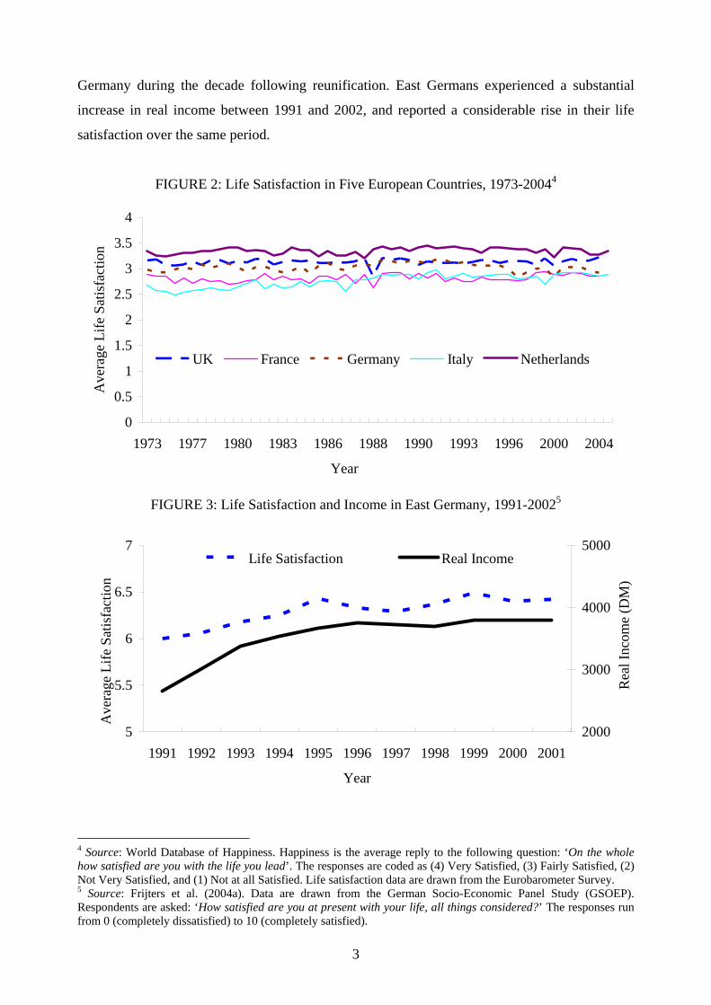
Germany during the decade following reunification. East Germans experienced a substantial
increase in real income between 1991 and 2002, and reported a considerable rise in their life
satisfaction over the same period.
FIGURE 2: Life Satisfaction in Five European Countries, 1973-20044
0
0.5
1
1.5
2
2.5
3
3.5
4
1973 1977 1980 1983 1986 1988 1990 1993 1996 2000 2004
Year
Ave
rage
Life
Sat
isfa
ctio
n
UK France Germany Italy Netherlands
FIGURE 3: Life Satisfaction and Income in East Germany, 1991-20025
5
5.5
6
6.5
7
1991 1992 1993 1994 1995 1996 1997 1998 1999 2000 2001
Year
Ave
rage
Life
Sat
isfa
ctio
n
2000
3000
4000
5000
Rea
l Inc
ome
(DM
)
Life Satisfaction Real Income
4 Source: World Database of Happiness. Happiness is the average reply to the following question: ‘On the whole how satisfied are you with the life you lead’. The responses are coded as (4) Very Satisfied, (3) Fairly Satisfied, (2) Not Very Satisfied, and (1) Not at all Satisfied. Life satisfaction data are drawn from the Eurobarometer Survey. 5 Source: Frijters et al. (2004a). Data are drawn from the German Socio-Economic Panel Study (GSOEP). Respondents are asked: ‘How satisfied are you at present with your life, all things considered?’ The responses run from 0 (completely dissatisfied) to 10 (completely satisfied).
3
However, we should be cautious in concluding from these graphs, which illustrate bivariate
correlations, that income does not buy happiness in the developed world. A parallel body of
work has produced what is now a large amount of evidence suggesting that money does matter.
There are three stylised facts in this second literature.
1) A regression of happiness on income using cross-section survey data from one country (with
or without standard demographic controls) generally produces a significant positive estimated
coefficient on income. This holds for both developed (see, for example, Blanchflower and
Oswald, 2004; Shields and Wheatley Price, 2005) and developing (Graham and Pettinato, 2002;
Lelkes, 2006) countries. However, the income-happiness slope is larger in developing or
transition than in developed economies.
2) Recent work has used panel data to control for unobserved individual fixed effects, such as
personality traits, and concludes that changes in real incomes are correlated with changes in
happiness (see, for example, Winkelmann and Winkelmann, 1998; Ravallion and Lokshin, 2002;
Ferrer-i-Carbonell and Frijters, 2004; Senik, 2004; Ferrer-i-Carbonell, 2005; Clark et al., 2005).
Further, a number of these studies have been able to utilise exogenous variations in income to
establish more firmly the causal effect of income on happiness (e.g. Gardner and Oswald, 2007;
Frijters et al., 2004a, 2004b, 2006). It is again the case that income has a larger effect in
transition than in developed countries. In addition, the slope of the income-happiness
relationship is not necessarily the same between groups (Clark et al., 2005; Frijters et al., 2004a;
Lelkes, 2006).
3) Recent detailed studies of the ‘macroeconomics of happiness’ using very large samples and
cross-time cross-country models that control for country fixed-effects, have shown that
happiness co-moves with macroeconomic variables including GDP, GDP growth and inflation
(see, for example, Di Tella et al., 2003; Helliwell, 2003; Alesina et al., 2004). A useful set of
recent figures is to be found in Leigh and Wolfers (2006).
The bulk of the evidence in 1) – 3) thus suggests that income does raise happiness. One of
the key challenges for the nascent economics of happiness literature is therefore to render the
significant income coefficient found in much of empirical literature consistent with the time
profiles shown in Figures 1, 2 and 3, and to identify the ensuing implications of the fundamental
income-happiness relationship for both economic theory and policy design.
4
This paper attempts to respond to that challenge. Our answer is based on the concept of
income comparisons – both to others in the relevant reference group (social comparisons) and to
oneself in the past (adaptation or habituation). In Section 2, we provide a unified account of the
observed income-happiness gradients in both the micro and macro literature by presenting them
as straightforward extensions of the textbook utility function.
We then turn to the question of micro-economic evidence that is consistent with the
presence of income comparisons in the utility function. The recent growth of the empirical
literature on income and happiness has produced much information in this respect. We
summarise these new findings in Section 3, especially focusing on studies that have used panel
data from surveys such as the British Household Panel Survey (BHPS), the German Socio-
Economic Panel Study (GSOEP) and the Russian Longitudinal Monitoring Survey (RLMS).
These panel studies allow researchers to track individuals’ income and happiness over long
periods (now over 20 years in the case of the GSOEP) and to control for individual fixed traits,
the latter having been shown to be crucial for the empirical modelling of subjective well-being
(Ferrer-i-Carbonell and Frijters, 2004).
In Section 4 we directly address the question, ‘Is happiness related to utility’? In particular,
we consider a number of findings from the analysis of objective data, experimental economics,
and neuroscience which are consistent with relative income playing a role in the individual
utility function. However, we also underline a number of possible objections to the use of
happiness data to reveal such income comparisons. Section 5 then highlights some of the main
implications of income comparisons for a range of issues relating to economic theory and policy
design. The economic issues we focus on include many of the central concerns of economics:
consumption, investment, economic growth, savings, taxation, labour supply, wages and
migration. Finally, section 6 concludes.
2. Explaining the Easterlin Paradox by Relative Income
The explanation of the Easterlin paradox detailed in this paper rests on the ways in which
income translates into utility. It is important to be clear about the logical step that we are taking
here. While the paradox is couched in terms of income and happiness, we are going to appeal to
a specific type of utility function to account for it. In other words, we imagine that happiness
scores provide information about utility. We will maintain this hypothesis over both this section
and the micro-level income and happiness results described in Section 3. Section 4 will then
explicitly set out the evidence linking happiness and utility.
5
In this section we consider the implications of relative or comparison income terms in the
individual utility function. These comparisons may concern others, or oneself in the past,
evoking the possibility that individuals adapt or ‘get used to’ their changing income (Easterlin,
2001). Both of these types of comparison can be presented as simple extensions to the standard
economics textbook utility function. Consider a utility function of the form:
(1) *1 2 3 1( ( ), ( | ), u ( , ))t t t t tU U u Y u Y Y T l Z= t−
3
t
where is a common function over all individuals indicating how the sub-utilities
are combined into final utility U; the subscript t refers to time.
(.)U
1 2, , and u u u
In this specification, is the vector of incomes from t=0 to t and can be thought of
as the classic function showing utility from consumption, which is increasing at a decreasing
rate in its argument. As we are thinking of a vector of incomes in general, past incomes may
affect current consumption, for example via wealth. In a one-period model, or in a model
without savings, income will equal consumption , so that
tY ty 1(.)u
tc 1 1 1( ) ( ) ( )t tu Y u y u c= = . The sub-
utility function picks up the influence of leisure, (3( ,t tu T l Z− 1 ) )tT l− , with denoting hours at
work, and a vector of other socio-economic and demographic variables,
tl
1tZ .
The empirical application of (1) typically appeals only to current values of Yt and a partial
log-linear specification:
* '1 2ln( ) ln( / )t t t tU y y y tZβ β γ= + + (2)
where is usually a measure of real individual or household income, is some specific
reference income, and Z includes both demographics and hours of work.
ty *ty
While the first and third parts of the utility function in (1) are standard, the second is less so,
and shows the influence of status or habituation. The economic analysis of such relative income
effects (or more generally, interdependent preferences) can be dated back to at least Veblen
(1899), and then Duesenberry (1949). More recent contributions include Pollak (1976), Frank
(1985) and Elster and Roemer (1991)
The variable is often called ‘reference group’ or ‘comparison’ income, and the ratio
Yt/Y*t is called ‘relative’ income. Any empirical test of such a utility function will require us to
specify individual reference groups. In this respect, we can distinguish between internal
*tY
6
reference points, such as own past income or expected future income, and external reference
points, where comparisons refer to distinct demographic groups such as own family, other
workers at the individual’s place of employment, people in the same neighbourhood, region,
country, or even people across a whole set of countries. With external reference points,
can be interpreted as the 'status return' from income, or the positional or conspicuous
consumption aspect of income.6 This status function is assumed to increase at a decreasing rate
in , but decrease at an increasing rate in . The status function is homogeneous of degree
zero, so that : status is unaffected by proportional increases in income
and reference income. In many cases,
*2 ( | )t tu Y Y
tY *tY
*2 2( | ) ( |t t t tu aY aY u Y Y= * )
*2 ( | ) /t t tu Y Y c c= t , where tc is average reference group
consumption, but the formulation is sufficiently general to encompass the bulk of the
specifications used in the literature.
In the following sub-sections, we show how this basic model can easily explain the Easterlin
paradox, first considering comparisons to others, and then comparisons to one’s past.
2.1 Social comparisons
To illustrate the main forces at work when individuals compare to others, consider the following
stylised implication of the relationship between income and happiness across countries when: i)
income is the only systematic difference between countries (so that we can relegate u3 in
equation (1) to a constant and ignore it); and ii) reference income is average income within the
country. This case is depicted in Figure 4, for the function: 1 2 ln( / )ii i
i
yU yy A
β β= ++ iy , with
iy being average income in the country where individual i lives, and A being a positive constant.
The functional form here is deliberately chosen to ensure that the benefit of an across-the-board
proportional rise in income tends to zero as income goes to infinity: a general rise in income
leaves the second term unchanged, and has an effect on the first term which tends to zero as
income increases. Note that this is not true of the formulation in (2) where a growth in log-
income by x will increase utility by x 1β for any level of income.
The main prediction of this model is that the gradient between income and happiness will be
steeper within a country at a point in time than over time by country. This is due to the status
benefit of high income within a country. Crucially, however, this status benefit has no aggregate
impact on country-level happiness (in this model, the more status one person has, the less others
6 Others’ income might also matter for non-comparison reasons: for example if a general rise in income leads to higher prices. We only consider social comparisons here.
7
have: status is a zero-sum game). Over time in a given country, the only effect of income on
aggregate happiness will be via the consumption component of the utility function (u1).
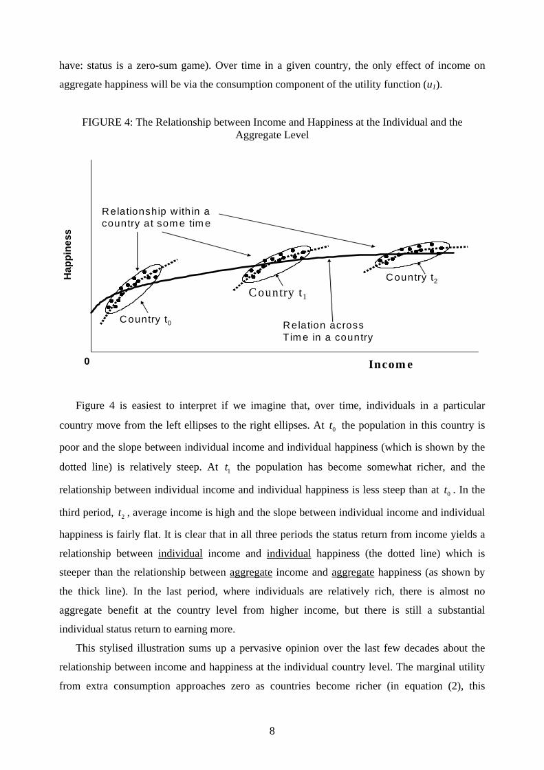
FIGURE 4: The Relationship between Income and Happiness at the Individual and the Aggregate Level
0
Hap
pine
ss
Relation across Tim e in a country
Country t0
Incom e
Country t2
Country t1
Relationship w ith in a country at som e tim e
Figure 4 is easiest to interpret if we imagine that, over time, individuals in a particular
country move from the left ellipses to the right ellipses. At the population in this country is
poor and the slope between individual income and individual happiness (which is shown by the
dotted line) is relatively steep. At the population has become somewhat richer, and the
relationship between individual income and individual happiness is less steep than at . In the
third period, , average income is high and the slope between individual income and individual
happiness is fairly flat. It is clear that in all three periods the status return from income yields a
relationship between individual
0t
1t
0t
2t
income and individual happiness (the dotted line) which is
steeper than the relationship between aggregate income and aggregate happiness (as shown by
the thick line). In the last period, where individuals are relatively rich, there is almost no
aggregate benefit at the country level from higher income, but there is still a substantial
individual status return to earning more.
This stylised illustration sums up a pervasive opinion over the last few decades about the
relationship between income and happiness at the individual country level. The marginal utility
from extra consumption approaches zero as countries become richer (in equation (2), this
8
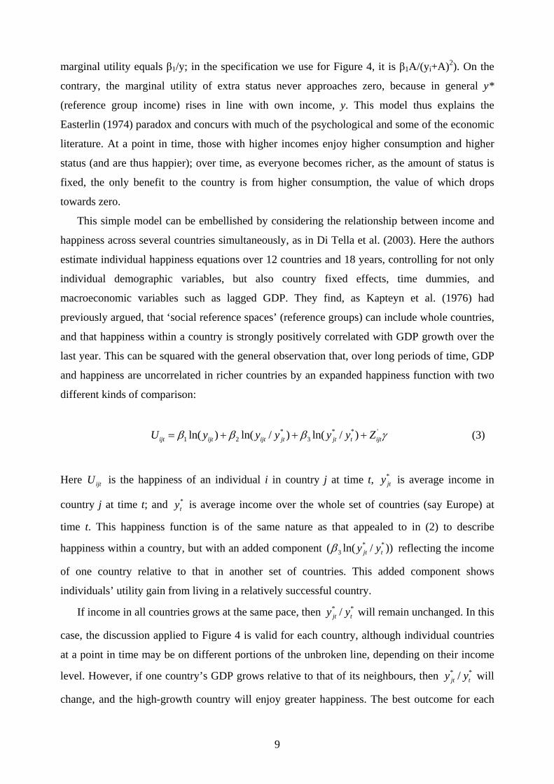
marginal utility equals β1/y; in the specification we use for Figure 4, it is β1A/(yi+A)2). On the
contrary, the marginal utility of extra status never approaches zero, because in general y*
(reference group income) rises in line with own income, y. This model thus explains the
Easterlin (1974) paradox and concurs with much of the psychological and some of the economic
literature. At a point in time, those with higher incomes enjoy higher consumption and higher
status (and are thus happier); over time, as everyone becomes richer, as the amount of status is
fixed, the only benefit to the country is from higher consumption, the value of which drops
towards zero.
This simple model can be embellished by considering the relationship between income and
happiness across several countries simultaneously, as in Di Tella et al. (2003). Here the authors
estimate individual happiness equations over 12 countries and 18 years, controlling for not only
individual demographic variables, but also country fixed effects, time dummies, and
macroeconomic variables such as lagged GDP. They find, as Kapteyn et al. (1976) had
previously argued, that ‘social reference spaces’ (reference groups) can include whole countries,
and that happiness within a country is strongly positively correlated with GDP growth over the
last year. This can be squared with the general observation that, over long periods of time, GDP
and happiness are uncorrelated in richer countries by an expanded happiness function with two
different kinds of comparison:
* * *1 2 3ln( ) ln( / ) ln( / )ijt ijt ijt jt jt t ijtU y y y y y 'Zβ β β= + + + γ
*
*
(3)
Here is the happiness of an individual i in country j at time t, is average income in
country j at time t; and is average income over the whole set of countries (say Europe) at
time t. This happiness function is of the same nature as that appealed to in (2) to describe
happiness within a country, but with an added component reflecting the income
of one country relative to that in another set of countries. This added component shows
individuals’ utility gain from living in a relatively successful country.
ijtU *jty
*ty
* *3( ln( / ))jt ty yβ
If income in all countries grows at the same pace, then will remain unchanged. In this
case, the discussion applied to Figure 4 is valid for each country, although individual countries
at a point in time may be on different portions of the unbroken line, depending on their income
level. However, if one country’s GDP grows relative to that of its neighbours, then will
change, and the high-growth country will enjoy greater happiness. The best outcome for each
* /jt ty y
* /jt ty y
9
country is to have high income while its neighbours have low incomes. However, unless one
country can increasingly outstrip its neighbours, the additional benefit of more income is subject
to decreasing returns.7 This type of happiness function can help explain why countries are
locked in an arms race over growth, even though, on aggregate, that growth will only bring
utility via the consumption function. In each country the component produces a
strong relationship between GDP and happiness. However, analogously to the individual
argument within a country, the happiness return from being richer than other countries is, from
the world perspective, a zero-sum game.
* *3 ln( / )jt ty yβ
At the individual level, these kinds of status-races can lead to sub-optimal outcomes if they
crowd out non-status activities. This can be illustrated using the general (one-country) utility
function (1), where a higher income for individual i reduces the utility of everyone whose
reference group includes i. In the specification proposed, higher income comes about at the
expense of leisure time. Consider the parameterisation:
1 2ln( ) ln( / ) ln( / )it it it t it tU y y y T y wβ β γ= + + − (4)
where the expression ln( / )it tT y wγ − reflects the utility from leisure (which is written as T
minus the number of hours spent earning income at wage ). Figure 5 illustrates the
individual’s utility-maximising choice of income relative to that pertaining in the social
optimum (where status externalities are internalised).
ity tw
In this figure, the top curve shows it
it
dUdy
, the marginal utility to the individual of additional
labour income. This marginal utility is positive up to income Y2, at which point the detrimental
effect to the individual of less leisure is exactly balanced by the increased consumption and
higher status that come with more income. The lower curve in this figure represents
| t it t ity y y yit it
it t
U Uy y
=∂ ∂+
∂ ∂| = , which is the effect of additional income in the country when everyone’s
income increases at the same time (i.e. when all individuals make the same choice). This
effectively removes the status benefit of higher income. The second curve lies below the first
due to the negative externality of in the term ty 2 ln( / )it ty yβ . Individuals choose income of Y2,
where their marginal utility of income is zero, whereas the societal optimum, taking externalities
7 Note that if the ‘true’ happiness function does indeed depend (negatively) on some measure of reference group income, but we instead estimate a happiness equation that does not include y*, then the negative effect of higher levels of y* over time will show up as a negative time-trend (as in Di Tella et al., 2003).
10
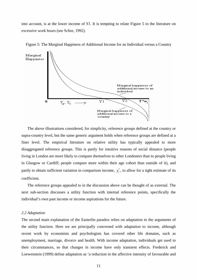
into account, is at the lower income of Y1. It is tempting to relate Figure 5 to the literature on
excessive work hours (see Schor, 1992).
Figure 5: The Marginal Happiness of Additional Income for an Individual versus a Country
The above illustrations considered, for simplicity, reference groups defined at the country or
supra-country level, but the same generic argument holds when reference groups are defined at a
finer level. The empirical literature on relative utility has typically appealed to more
disaggregated reference groups. This is partly for intuitive reasons of social distance (people
living in London are more likely to compare themselves to other Londoners than to people living
in Glasgow or Cardiff; people compare more within their age cohort than outside of it), and
partly to obtain sufficient variation in comparison income, , to allow for a tight estimate of its
coefficient.
*ty
The reference groups appealed to in the discussion above can be thought of as external. The
next sub-section discusses a utility function with internal reference points, specifically the
individual’s own past income or income aspirations for the future.
2.2 Adaptation
The second main explanation of the Easterlin paradox relies on adaptation to the arguments of
the utility function. Here we are principally concerned with adaptation to income, although
recent work by economists and psychologists has covered other life domains, such as
unemployment, marriage, divorce and health. With income adaptation, individuals get used to
their circumstances, so that changes in income have only transient effects. Frederick and
Loewenstein (1999) define adaptation as ‘a reduction in the affective intensity of favourable and
11
unfavourable circumstances’, and the concept of reversion back to some baseline hedonic level
following temporary highs and lows in happiness has been termed the ‘hedonic treadmill’
(Brickman and Campbell, 1971). Kimball and Willis (2006) provide a fuller review of work on
the psychology of adaptation and reference points.
From an economist’s point of view, a simple way of thinking of adaptation to income is in
terms of an internal backward-looking reference point. We thus remain in the general framework
of equation (2), but now consider that is formed from own past incomes. If the individual
compares her own income at time t to (a geometric average of) that earned over the past three
years, we would have:
*ty
*1 2
* 11 2 3
1 2 1 2 3
ln( ) ln( / ) '
( ) ( ) ( )
ln( ) [ln( ) ln( ) ln( ) (1 )ln( )] '
it it it t it
t it it it
it it it it it it it
U y y y Z
y y y y
U y y y y y Z
α γ α γ
β β γ
β β α γ α γ
− −− − −
− − −
= + +
=
= + − − − − − + γ
(5)
In the final utility function we have the logs of current income and income over the last three
periods.8 This equation can in principle be extended to include further lags of current income; if
aspirations are important (another internal reference point, but this time forward-looking) it may
also include expected future incomes. One of the main implications of this specification is that
the short-run effect of an increase in log income equals 1β + 2β whilst the long-run effect is only
1β . This is obviously analogous to the social comparison case, where the marginal utility of
higher income was greater when others’ income remained constant than when others’ income
rose in line. In terms of Figure 4, the short-run benefit of higher income is illustrated by the
dotted lines, whereas the (flatter) thick line shows the long-run benefit.
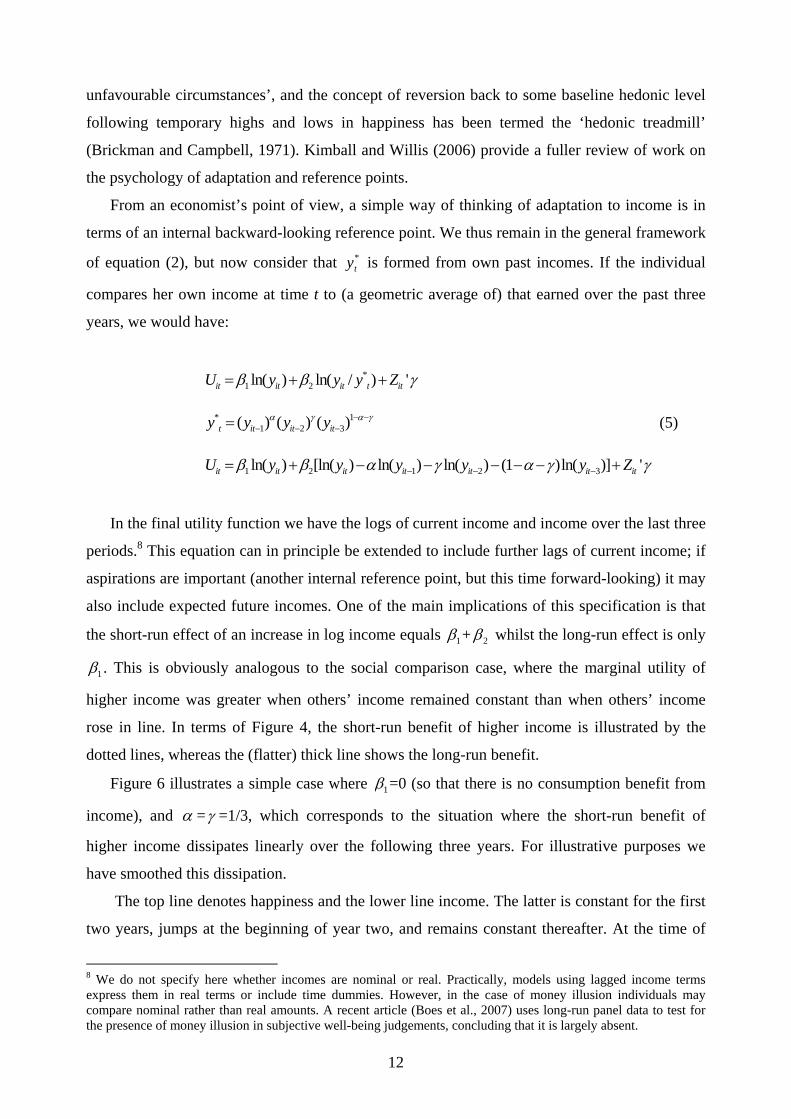
Figure 6 illustrates a simple case where 1β =0 (so that there is no consumption benefit from
income), and α =γ =1/3, which corresponds to the situation where the short-run benefit of
higher income dissipates linearly over the following three years. For illustrative purposes we
have smoothed this dissipation.
The top line denotes happiness and the lower line income. The latter is constant for the first
two years, jumps at the beginning of year two, and remains constant thereafter. At the time of
8 We do not specify here whether incomes are nominal or real. Practically, models using lagged income terms express them in real terms or include time dummies. However, in the case of money illusion individuals may compare nominal rather than real amounts. A recent article (Boes et al., 2007) uses long-run panel data to test for the presence of money illusion in subjective well-being judgements, concluding that it is largely absent.
12
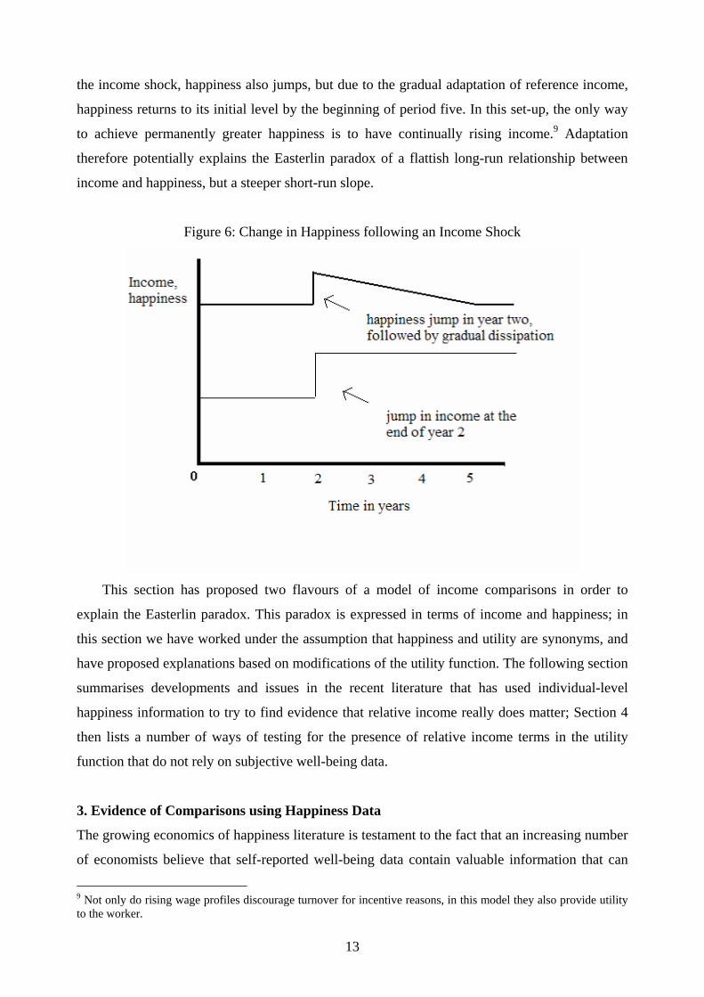
the income shock, happiness also jumps, but due to the gradual adaptation of reference income,
happiness returns to its initial level by the beginning of period five. In this set-up, the only way
to achieve permanently greater happiness is to have continually rising income.9 Adaptation
therefore potentially explains the Easterlin paradox of a flattish long-run relationship between
income and happiness, but a steeper short-run slope.
Figure 6: Change in Happiness following an Income Shock
This section has proposed two flavours of a model of income comparisons in order to
explain the Easterlin paradox. This paradox is expressed in terms of income and happiness; in
this section we have worked under the assumption that happiness and utility are synonyms, and
have proposed explanations based on modifications of the utility function. The following section
summarises developments and issues in the recent literature that has used individual-level
happiness information to try to find evidence that relative income really does matter; Section 4
then lists a number of ways of testing for the presence of relative income terms in the utility
function that do not rely on subjective well-being data.
3. Evidence of Comparisons using Happiness Data
The growing economics of happiness literature is testament to the fact that an increasing number
of economists believe that self-reported well-being data contain valuable information that can
9 Not only do rising wage profiles discourage turnover for incentive reasons, in this model they also provide utility to the worker.
13
complement our understanding of individual behaviour.10 In terms of the specific subject of this
review, happiness data are the cornerstone of the Easterlin paradox; this section asks whether the
same data can be used to resolve this paradox, by empirically demonstrating the importance of
social comparisons and adaptation. A rapidly-growing number of econometric studies have used
survey data on happiness or life satisfaction to evaluate the importance of ‘absolute’ versus
‘relative’ income. Under the maintained hypothesis that happiness is a good proxy measure of
utility, this corresponds to estimating the relative size of the coefficients β1 and β2 in equation
(2).
3.1 Happiness and social comparisons
All empirical tests of social comparisons over income, whether using happiness data or any
other approach, require candidate measures of . One such candidate is the income of ‘people
like me’ (e.g. those with the same age, education etc., who are doing the same kind of job). This
reference group income can be calculated in two different ways. We can first estimate wage
equations and then compute the predicted income of ‘someone like me’, where the regression
controls for individual characteristics such as age, sex, education and region, as in Clark and
Oswald (1996). Second, perhaps more simply, we can compute cell averages (for example,
average wage by region, sex and education). This latter calculation can either be carried out
within the dataset, or matched in from an external source.
*ty
A crucial issue in the econometric literature is that of identification: is typically estimated
as a linear function of some explanatory variables X1 in the wage equation approach. To then
identify the effect of on happiness, we need either exclusion restrictions (some variables
which appear in X1 but which do not enter the happiness equation), or identification directly
from the functional form (such as when the prediction of enters in a different functional form
in the happiness regression to the variables in X1). The cell average approach relies on a more
subtle exclusion restriction that individuals compare themselves only to the average income
within each cell.
*ty
*ty
*ty
The empirical literature mostly started by considering job satisfaction, reflecting economists’
interest in wages and the labour market, and perhaps also the original research carried out in
10 A search of ECONLIT for journal articles with either ‘Happiness’, ‘Life Satisfaction’ or ‘Well-being’ in the title, identifies 465 published articles between 1960 and 2006. Of these 363 (78%) have been published since 1995, 285 (61%) have been published since 2000, and one-third of the literature (37%, or 173 articles) has appeared in print in just the last three years.
14
industrial psychology, before moving on to global measures of well-being such as happiness and
life satisfaction.
Probably the first economist to estimate subjective well-being equations using both y and
was Dan Hamermesh (1977). Although Hamermesh's focus is upon occupational choice and the
effects of training in American data, and he does not discuss relative income in detail, his job
satisfaction regressions include the residual from a wage equation as an explanatory variable.
This residual, y- in our terminology, has a positive and significant effect on job satisfaction.
*ty
*ty
The regression approach of calculating the income of ‘people like me’ was also used by
Clark and Oswald (1996) on the first wave of British Household Panel Study (BHPS) data. The
estimated coefficients on income and comparison income in a job satisfaction equation are
statistically equal and opposite, which is consistent with a fully relative utility function: to
paraphrase Easterlin (1995), in these results increasing the income of all increases the happiness
of no-one. Lévy-Garboua and Montmarquette (2004), and Sloane and Williams (2000), using
Canadian and British data respectively, have also found evidence that econometrically-predicted
comparison income is negatively correlated with job satisfaction.
Articles which calculate comparison income as a cell average, rather than an econometric
prediction from individual data include Cappelli and Sherer (1988), who find that pay
satisfaction is negatively correlated with an outside ‘market wage’, calculated by averaging pay
for specific occupations in other firms (airlines, in this case). Clark and Oswald (1996) find a
negative relationship between job satisfaction in BHPS data and average earnings by hours of
work matched in from the UK Labour Force Survey.
Stepping outside of the realm of work, a number of recent papers have found comparison
income effects using cell means. Ferrer-i-Carbonell (2005) calculates comparison income as an
average within fifty cells defined by sex, age and education in six years of German GSOEP data;
McBride (2001) uses 1994 data from the General Social Survey, and defines comparison income
as average earnings of the individual’s cohort, defined as those who are between 5 years
younger and 5 years older than her. Blanchflower and Oswald (2004) use GSS data over the
period 1972-1998, with defined as average income by State. Luttmer (2005) also takes a
geographic approach to reference groups, and calculates average income by local area identified
in a number of waves of the US National Survey of Families and Households; this is shown to
be negatively correlated with respondents’ life satisfaction, conditional on their own income.
Graham and Felton (2006) replicate this finding across 18 Latin American countries. Helliwell
and Huang (2005) is in the same vein, calculating average household income by census tract in
Canadian GSS data. The estimated coefficient on this variable in life satisfaction equations is
*ty
15
negative, and equal in size to the positive coefficient on household income, suggesting that life
satisfaction is totally relative in income. As the estimated coefficient on income refers to β1+β2
in equation (2), and that on relative income to –β2, the finding that the coefficients are equal and
opposite is tantamount to saying that the consumption benefit of higher income (β1) is
essentially zero, which is consistent with Figures 1 to 3.
A novel paper dealing with social comparisons is Knight and Song (2006). This paper
appeals to cross-sectional information on 9,200 households in China, and thus refers to an
economy which is very different from the Europe-North America nexus which has so far
dominated the literature. The authors are not only able to identify which villages their
respondents came from, but also confirm that 70% of individuals indeed see their village as their
reference group (by simply asking them to whom they compare themselves), making their rural
sample well-suited to the question of how important reference groups really are. Controlling for
own income, and for village income, those respondents who say that their income was much
above the village average report far higher happiness than those who say that their income was
much below the village average. The difference between the two estimated coefficients implies a
happiness boost of one point, on a zero to four scale, making relative income the most important
right-hand side variable.
The above work considers as the income of ‘people like me’ or those living in the same
neighbourhood. Another potential peer group is those with whom the individual comes into
close daily contact: her family, friends and work colleagues. With respect to the latter, and
despite the current abundance of microeconomic data, very few papers have related individual
well-being to co-workers’ wages. One direct test is Brown et al. (2006), who use matched
employer-employee data from the British Workplace Employee Relations Survey (WERS).
Individuals were asked to report their satisfaction with the amount of influence they have, their
pay, their achievement, and the respect they receive. Controlling for own wage, the (normalised)
rank of the individual in the firm wage distribution is correlated positively and significantly with
all four measures of satisfaction (see their Table 6b).
*ty
The situation is equally sparse with respect to family and friends. Clark (1996a) uses BHPS
data to relate individual job satisfaction, conditional on own wage, to the wages of their partners
and the average wage of other household members. The results show that individuals do indeed
report lower job satisfaction scores the higher are the wages of other workers in the household.
McBride (2001) also introduces a family benchmark, appealing to the question in the GSS:
“compared to your parents when they were the age you are now, do you think your own
standard of living now is: much better, somewhat better, about the same, somewhat worse, or
16
much worse?”. While this is a valid approach, it is worth noting that it is perhaps a poor
candidate to explain the flat income-happiness relationship, as it remains fixed over time. In
other words, for the same individual, does not change with y, although new cohorts will
presumably have higher values of than will older cohorts.
*ty
*ty
Modelling the utility function via proxy variables, such as life or job satisfaction, is not the
only way to demonstrate social comparisons. One method that essentially inverts the question is
that of the Welfare Function of Income, associated with the Leyden school in the Netherlands,
and, particularly, with Bernard van Praag. This predates the work on satisfaction by some years,
with the first published article being Van Praag (1971). This project involved asking individuals
to assign income levels (per period) to six different verbal labels (such as "excellent", "good",
"sufficient" and "bad") and then, based on the values given, estimating for each individual a
lognormal "Welfare Function of Income". The resulting individual estimated means (µ) and
variances (σ) were then used as dependent variables in regressions which sought to explain
which types of individuals require a higher level of income to be satisfied, and which individuals
have valuations that are more sensitive to changes in income.
The results using cross-country data produced a number of important findings. In terms of
this paper’s subject, we would like to know who has a higher value of µ (i.e. who needs more
money to be satisfied?). Comparisons to others were analysed via the inclusion in the
regressions of reference group income (usually cell average income over age, education and
certain other individual or job characteristics) as a right-hand side variable. The empirical results
(for example, Hagenaars, 1986; and Van de Stadt et al., 1985) show that, ceteris paribus, the
higher is the reference group's income, the higher are the levels of income assigned by
individuals to the six verbal labels, as social comparisons over income would imply.
One of the very few papers ever to appeal to respondent-defined (rather than researcher-
defined) reference groups is Melenberg (1992). He uses 1985 and 1986 Dutch Socio-Economic
Panel data in which individuals are asked about their social environment – the “people whom
you meet frequently, like friends, neighbours, acquaintances or possibly people you meet at
work”. Respondents are asked to indicate the average age, household size, income, education
and labour force status in this group. Melenberg shows that the average income of this
(respondent-defined) reference group is positively and significantly correlated with the estimate
of µ from the WFI: those who associate with higher-earners need more money in order to
describe their income as good or adequate.
17

3.2 Happiness and adaptation
There is a large literature in psychology that deals with the general issue of adaptation in many
life domains (see Frederick and Loewenstein, 1999), but only a very few studies have focused
on income adaptation (see the work reviewed on their page 313). Perhaps the most famous
example is that of Brickman et al. (1978), who show using a very small sample of lottery
winners (n=22) that this group with their positive income shock do not have significantly higher
life satisfaction than a control group.11 They propose an explanation based on the twin concepts
of contrast (i.e. winning money opens up new pleasures but also makes existing pleasures less
enjoyable) and habituation (winners get used to a new standard of living). More recent examples
of adaptation in non-monetary spheres are Lucas et al. (2003) and Lucas (2005) with respect to
marriage and divorce, Wu (2001) and Oswald and Powdthavee (2005) for adaptation to illness
or disability, and Lucas et al. (2004) regarding unemployment.
Here we are especially interested in adaptation to income changes. One early article is
Inglehart and Rabier (1986), who use pooled Eurobarometer data from ten Western European
countries between 1973 and 1983 to show that life satisfaction and happiness scores are
essentially unrelated to the level of current income, but are positively correlated with a measure
of change in financial position over the past twelve months. Their conclusion is that aspirations
adapt to circumstances, such that, in the long run, stable characteristics do not affect well-being.
In the same tradition, Clark (1999) uses two waves of BHPS data to look at the relationship
between workers’ job satisfaction and their current and past labour income. The panel nature of
the BHPS makes it possible to concentrate on individuals who stay in the same firm, and in the
same position (i.e. have not been promoted or moved job in any other way). Both current and
past labour income and hours are used as explanatory variables. Past income attracts a negative
coefficient in the job satisfaction equation, and past hours a positive coefficient, consistent with
a utility function that depends on changes in these variables. The data suggest a completely
relative function, with job satisfaction depending only on the annual change in the hourly wage.
Grund and Sliwka (2003) find similar results in German GSOEP panel data. Weinzierl (2005)
introduces both past income and reference group income (calculated as a cell mean by gender,
age and education) in life satisfaction equations using the GSOEP data, and finds negative and
significant coefficients for both. Last, Burchardt (2005) finds evidence of adaptation in income
satisfaction in ten years of BHPS data, with a suggestion of greater adaptation to rises in income
than to falls in income.
11 Important though this paper is, it is worth noting that the paper is cross-section ex post: no shock is observed. Further, winners were actually more satisfied than non-winners, but given the small sample size the difference was not significant.
18
A recent detailed study of life satisfaction and income adaptation was carried out by Di Tella
et al. (2005), who analyse longitudinal data for around 8,000 individuals drawn from the West
German sample of the GSOEP over the period 1984 to 2000. They find that the effect of an
income increase after four years is only about 42% of the effect after one year: the majority of
the short-term effect of income vanishes over time.
An alternative to using individual income, and its lags, is to concentrate on aggregate
income. Di Tella et al. (2003) examine individual happiness in data covering 18 years across 12
European countries, and argue that some of their results on current and lagged GDP per capita
show that ‘bursts of GDP produce temporarily higher happiness’ (p.817).
The Leyden Group (e.g. Hagenaars, 1986; Van de Stadt et al., 1985; Plug, 1997; and Van
Praag, 1971; for a review see Van Praag and Frijters, 1999) explicitly attempted to measure the
degree of adaptation to income. The cornerstone of this empirical work is the Welfare Function
of Income, as described in Section 3.1 above. Questions permitting a direct estimate of the
income needed to achieve a fixed level of welfare were posed in the GSOEP, in the EUROSTAT
surveys of the 1980s, in Russian panels, in the Dutch Socio-Economic Panel, and in various
other surveys. The relationship between this required income level and the individual’s past
income can then be seen as a direct measure of adaptation, or as Van Praag (1971) calls it,
‘preference drift’. The stylised finding for about 20 European countries is that a $1 increase in
the income of a household leads to a 60 cents increase (within about 2 years12) in what people
consider to be a ‘excellent’, ‘good’, ‘sufficient’ and ‘bad’ income. Income adaptation is
therefore high, but not complete in this methodology.
The individual-level reports match up with what is found at the aggregate level concerning
subjective poverty (having an income lower than that was deemed minimal). European countries
which are on average poorer (such as Greece and Portugal) are found to have many more
respondents whose own income was below an insufficient level than richer European countries
such as Germany or Switzerland. For instance, subjective poverty was about 3% in West
Germany in the 1990s, but up to 90% in Russia in 1993 (Van Praag and Frijters, 1999).
A second individual-level reference point is aspirations. The concept is the same as that of
adaptation: if aspirations rise with own actual income, then the effect of income on happiness
will be muted.
As might be imagined, there is only relatively little work here, as it is difficult to know how
12 The 60% finding was initially based on cross-sectional within-country data, but has since also been found to hold over time. See Van Praag and Frijters, 1999, for specific longitudinal results.
19
to accurately measure income aspirations.13 Easterlin (2005b) uses direct measures to show that
material aspirations (the big-ticket consumer items that make up the good life) seem to increase
in line with ownership of such consumer items. However, this is not true with respect to
marriage, where over forty percent of those who have been single their entire lives, and are aged
45 and over, cite a happy marriage as part of the good life. Two recent papers have taken
different approaches to measuring income aspirations, and relating them to subjective well-
being. Stutzer (2004) combines the analysis of subjective data with the income evaluation
approach of the Leyden school, by using the answer to the Minimum Income Question14 as a
measure of individual income aspirations (and thus one measure of y*) in a life satisfaction
equation.
McBride (2006) introduces a novel way of calculating aspirations directly in a matching
pennies game, where individuals play against computers. The computer chooses heads or tails
according to (known) probability distributions (for example 80% heads, 20% tails). After each
round of playing, individuals report their satisfaction with the outcome. McBride’s first
contribution is to introduce social comparisons in some of the treatments (by telling the
individual the outcomes of the other players). Second, he is able to identify an aspiration effect
by varying the heads and tails probabilities played by the computer. Each subject has five
pennies to play. When paired with a 80% heads, 20% tails computer, the best strategy is to
always play heads, which gives an expected payoff of four pennies. When paired with a 65%
heads, 35% tails computer, the best strategy is still to always play heads, but now the expected
payoff is only 3.25 pennies. By manipulating the probabilities, McBride creates variations in
aspirations. The empirical analysis shows that satisfaction is a) higher the more one wins, b)
lower the more others win, and c) lower the higher was the aspiration level.
3.3 Do social comparisons and adaptation explain the Easterlin ‘Paradox’?
Some of the research that we have cited above allows us to undertake tentative back-of-the-
envelope calculations of the relationship between income and happiness. For example, we can
take the key finding in the Leyden literature that adaptation over time accounts for around 60%
of the effect of income (i.e. income’s long-run effect is only 40% of its short-run effect), which
corresponds closely to the results in Di Tella et al. (2005). We can further appeal to one of the
best sources of information on the extent of social comparisons, Knight and Song’s (2006)
13 Suggestive indirect evidence is easier to find. Clark (1997), for example, suggests that the stubbornly higher job satisfaction reported by British women in BHPS data might partly reflect their lower expectations. 14 Where individuals are asked to indicate the sum per period they think is the absolute minimum net family income their family requires to make ends meet. This was introduced in Goedhart et al. (1977).
20
finding that relative income is at least twice as important for individual happiness as actual
income, even in poor regions (in their case rural China). Together, this suggests a utility function
in which 2/3 of aggregate income has no effect because it is status-related, and thus disappears
in a zero-sum game, and where 60% of the effect at the individual level evaporates within two
years due to adaptation. Hence only around 13% of the initial individual effect will survive in
the long run at the aggregate level.15 Precisely such a happiness function is shown in Figure 4,
which represents the basic aspects of the Easterlin ‘Paradox’ shown in Figures 1 and 2. It is
possible that even this small positive long-run effect may be an overestimate, as new generations
or cohorts may start with higher aspiration levels than older generations. Any such
intergenerational adaptation of aspirations would further diminish the long-run aggregate effect
of higher income, but is at present still ill-accounted for in the literature.
3.4 Key challenges for empirical work
Akin to many areas of applied economics, establishing the nature of the empirical relationship
between income and happiness faces a number of challenges, even if we presume that happiness
is perfectly measured and conforms to experienced utility. Here we highlight a number of the
main difficulties.
Firstly, economic theory often dictates that the relevant measure of welfare is consumption,
not income, and that income in happiness regressions is only a noisy proxy for consumption
(Weinzierl, 2005). As such researchers will tend to underestimate the importance of material
circumstances on happiness. Headey and Wooden (2004) go some way toward to addressing this
issue. They use Australian panel data (HILDA) and find that ‘net worth’, which is arguably a
better proxy for current consumption than a transitory measure of income, matters broadly at
least as much as does income in determining happiness. As they conclude, ‘the unimportance of
material circumstances has been exaggerated’. The main reasons why consumption and income
may differ are the consumption that individuals obtain directly from others, and deferred
consumption via savings. Regarding the first of these, individuals in developed economies are
provided with a great deal of consumption goods via the State, such as education, health care,
and transfers-in-kind, which are only rarely taken into account in empirical estimations. If
public-goods consumption is not directly measured, then proxy variables, such as local area or
country income, which are related to public goods via taxation, will attract positive coefficients.
15 These percentage figures are remarkably close to the estimates of interdependent preferences and habit-formation in Ravina (2005), using panel data on US credit-card holders’ consumption expenditure. Weinzierl (2005) includes both cell-average reference group income (by age, sex and education) and lagged income in a life satisfaction equation. The estimated coefficients imply that satisfaction is completely relative with respect to income. We do not know, however, whether this definition of the reference group is apt.
21
This will pollute the status effect of aggregate incomes on happiness, so that the coefficient on
aggregate income in happiness regressions will suffer from upward bias if public good
consumption is not taken into account.
Even measuring personal consumption is difficult. Not only do individuals likely have
trouble remembering how much of their income they have saved in financial assets, but more
fundamentally it is difficult to establish empirically a clean borderline between purchases that
have only current consumption benefits and purchases with some future consumption benefit.
How much of a car or a house purchased today should be counted as current consumption and
how much as future consumption? How much of education is current status consumption, and
how much investment? Issues such as these, which relate to the majority of major purchase
decisions, are very tricky and create a significant rift between theoretical models and empirical
estimates of consumption. If we do use individual income instead of consumption in happiness
regressions, we should remember that income is an overestimate of what is consumed when
young (when we save) and an underestimate when old (when we dis-save). Forcing income to
have a single coefficient over all ages then implies an upward bias in the effect of age on
happiness.
The second major empirical difficulty, as already briefly mentioned above, is to correctly
identify reference groups, especially when individuals move a great deal in their lifetimes and
reside in high population-density areas. Only very few studies ask individuals about their
reference groups, rather than simply imposing one. As noted in Section 3.1, Melenberg (1992)
asks respondents directly about the income of the people with whom they interact often. We are
only aware of one study where respondents were given a list of options and asked to explicitly
state to whom they compare themselves. As mentioned above, in Knight and Song (2006) 68%
of survey respondents in China reported that their main comparison group consisted of
individuals in their own village, whereas only 11% stated that their main comparison group
consisted of individuals from outside of the village.16
Almost all of the rest of the literature has resorted to assuming a particular reference income,
and therefore inserts variables into the empirical model such as the individual’s predicted
income according to her characteristics or the income in some geographical area, which is less
convincing. The generic problem with using constructed reference groups is that they might pick
up effects other than social comparison: average income by geographical area will likely also
16 Wave 3 (2006) of the European Social Survey will go some way to filling this lacuna. Individuals are first asked “How important is it to you to compare your income with other people’s incomes?” They are then asked “Whose income would you be most likely to compare your own with?”, with responses on a showcard of Work colleagues, Family members, Friends, and Others.
22
measure local public good consumption; co-workers’ income may pick up measurement error in
own reported income; and income predicted from a regression may reflect own expected future
income. Therefore, in the absence of accurate information about reference groups, we should be
cautious in claiming to have evaluated the importance of social comparisons over income from
happiness data.
A third point is that the group of individuals (or countries), to whom individuals compare is
assumed to be exogenous, and not a matter of choice. Falk and Knell (2004) ask what happens if
individuals can partly choose their reference groups.17 To obtain interior solutions for this
choice, the psychological literature has distinguished between ‘self-enhancement’ and ‘self
improvement’ motives. A concern for status implies that individuals prefer low-income
reference groups: this is ‘self-enhancement’. In the extreme, everyone would compare
themselves to the poorest individual(s), which clearly does not fit reality. The ‘self
improvement’ motive then posits some indirect benefit to having a higher-income reference
group. One such benefit works through the cost of effort: “people perform better and are more
successful if they set themselves high goals or compare with high reference standards” (p. 421).
The main result of Falk and Knell’s model is that the endogenously-chosen reference level
increases with individual ability (as measured by the rate of transformation of effort into output),
so that higher-ability individuals will choose higher-income reference groups. The choice of
reference group will then be based on the trade-off between status and the higher output that
comes from lower effort cost. Rablen (2006) considers an explicit dynamic model where agents
face self-control problems (there are future benefits from current effort). He shows that the
‘planner’, who maximises the individual's intertemporal utility, may find it optimal to introduce
a reference level into the utility function. The optimum reference level comes from the trade-off
between the direct utility cost of evaluating outcomes relatively and the future benefits from
higher current effort levels. Stark (2005, 2006a) has written a number of papers which appeal to
reference-group choice to better explain the migration decisions of heterogenous individuals. It
is important to note, however, that the empirical happiness literature is still in its infancy on this
issue.
A fourth challenge concerns the timing of income changes: the empirical prediction from the
loss-aversion hypothesis of Tversky and Kahneman (1991) is that the absolute effect of a loss of
one dollar, from an initial reference position, on individual happiness is greater than the effect of
a gain of one dollar. Any test of this prediction, which is highly relevant for many economic
17 A related question is treated in Oxoby (2004): what if individuals can choose the domains over which status comparisons take place?
23
phenomena (see Section 5), will require precise observation of the timing of both income
movements and reference income movements. Panel data, in which individuals are typically
interviewed only once per year, is consequently severely limited in its ability to distinguish
asymmetric happiness responses to incomes that are above and below the reference position. At
present, only experiments can address this asymmetry, but even these face well-known
limitations: experimental subjects are very often non-representative; the laboratory situation
itself may lack realism; and laboratory experiments on social phenomena are inherently
unsuitable for the measure of meaningful adaptation (such as the adaptation of reference groups)
as subjects cannot be kept in the laboratory for sufficiently long periods of time. Until we can
better track movements in both income and reference income, the loss-aversion hypothesis will
remain difficult to verify in this literature.
A fifth challenge is to deal with the issue of missing variables. No data set has all the
variables one might wish and their absence often leads to problems. Missing variables lead on to
the issues of the endogeneity of key variables and spurious relations between income and
happiness, and the problem of slope heterogeneity.
The first effect of missing variables is to render income potentially endogenous. It seems
plausible that happy people, or, equivalently, individuals with ‘happy’ personality traits, are
more likely to obtain better jobs (see Graham et al., 2004, and Lyubomirsky et al., 2005). Barker
(2005) similarly concludes that many later life outcomes depend on adverse influences during
early development, and specifically links both income and depression to birth size. The lack of
personality traits and early life influence variables in the data then implies that income is
endogenous. Drawing on these arguments, Ferrer-i-Carbonell and Frijters (2004) find in GSOEP
data that the partial correlation coefficient between changes in income and changes in happiness
is smaller than that between levels of income and levels of happiness. They advocate panel data
techniques to account for unobserved fixed individual traits that produce endogeneity problems.
However, even fixed-effect estimation will not identify time-varying factors that lead to both
greater happiness and higher income, producing spurious correlation. Good health, which allows
individuals to obtain better jobs and increases well-being, is a good candidate for a missing
factor that may lead to such a spurious correlation; marital stability and good relations with co-
workers are other possibilities. While the omission of these types of variable in happiness
regressions leads to an upward bias on the income coefficient, the reverse holds with respect to
variables that are themselves influenced by income and which are included as separate
regressors in a happiness regression. Health again fits the bill, as does housing and even marital
status: these outcomes are improved by higher incomes but are included in the regression as
24
exogenous factors, producing a smaller estimate on the income coefficient. The balance of such
conflicting effects is hard to predict.
Recent years have seen a number of papers appealing to natural experiments to skirt the
issue of endogeneity by providing some exogenous variation in income.18 Frijters et al. (2004a,
2004b, 2006) consider the large changes in real incomes observed in East Germany (following
reunification) and Russia (following transition) as exogenous, and find a greater effect of
income on happiness than in much of the existing literature. Gardner and Oswald (2007) use
information on lottery winnings in the BHPS as reflecting exogenous income movements. In
both level and panel equations, lottery winnings are found to significantly reduce mental stress
scores. It is worth underlining that natural data will only very rarely produce truly exogenous
income movements, although this is an issue for all work in applied microeconomics for which
income is important.
Missing variables at the aggregate level are important since any variable that correlates
positively with income and negatively with happiness may, if excluded from the data, give the
false impression that income does not lead to greater happiness and would thus be able to
explain the Easterlin Paradox. Some candidates which might spring to mind in this context are
pollution, (lower) social capital, and hours of work. Can any of these indeed explain why growth
is not making us happier? Probably the most detailed attempt at tackling this research question is
Di Tella and MacCulloch (2005a) using 23 years of Eurobarometer data and 28 years of
American GSS data. They examine a series of potential omitted variables which could explain
why increasing income has not led to more happiness. These are life expectancy, pollution
(measured as kilograms of Sulphur Oxide emissions per capita), unemployment and inflation,
hours worked, the divorce rate, crime and income inequality. Their empirical results show that
most of these are indeed correlated with life satisfaction in the expected manner. However, their
inclusion as right-hand side variables does not explain why rising income has not produced
rising well-being because, like income, these additional variables have mostly also improved
over time without increasing happiness: in their own words ‘introducing omitted variables
worsens the income-without-happiness paradox’.
Missing variables may also lead to different individuals having a different marginal benefit
from income i.e. ‘slope heterogeneity’. Presuming the same coefficient on income over the
whole sample may not be appropriate if there are important interacting variables omitted from
18 An alternative is to instrument income, although the task of finding instruments which affect income but not subjective well-being is a hard one. Lydon and Chevalier (2001) instrument income via spousal characteristics in a sample of UK University graduates, which leads to a doubling of the size of the income coefficient in a job satisfaction equation.
25
the data. Has the literature found any such interacting variables? The answer appears to be yes: a
recent example is Lelkes (2006), who shows that the religious were less affected, in life
satisfaction terms, by income movements during economic transition in Hungary. If religiosity
were a missing variable in this example, there would have been slope heterogeneity on
unobservables in Hungary. Smith et al. (2005) propose the same type of mediating relationship
for health. Clark et al. (2005) argue that such slope heterogeneity is likely to be present in many
more settings and propose to identify it on functional form assumptions on the error term and the
allowed types of slope heterogeneity. They use latent class techniques applied to three waves of
European Community Household Panel data to identify four different classes, in terms of both
intercept and the estimated coefficient on income in financial satisfaction equations.
A sixth and final challenge is the issue of the estimation method. Frey and Stutzer’s (2002a)
plea for greater use of panel techniques to overcome some of the missing variables problems
signalled above has largely been heeded. However, little attention has been paid to the exact
specification of the independent variables and one can think of many non-linearities that may be
important in actual work but that are usually ignored. In particular, the consensus use of log
income in well-being equations may hide important departures from log-linearity. In particular,
it may miss the presence of kinks, not only over time (as in loss-aversion), but also regarding
comparisons to others: is the return to having one dollar more than the neighbour the exact
opposite of having one dollar less? Better data and more flexible estimation techniques are
needed to address this challenge.
4. Is Happiness Related to Utility?
In this section we ask what basis there is for believing that happiness is a reasonable measure of
the economic notion of (decision) utility, i.e. the thing whose maximisation leads to choice
behaviour. It is, of course, surprisingly difficult to say whether any given series of numbers
conforms to utility or not. The full scale of the identification problem can be gauged by
reflecting on the two requirements that (decision) utility must fulfil in textbook treatments:
1. Utility guides individual choice in the sense that choices serve to maximise the expected
stream of utility.
2. Utility itself is the outcome of both choices and chance factors that were outside the
control of the individual but whose possibility was taken into account when decisions
were made.
26
The first identification problem is that in practice we are not able to say with any precision
what choices individuals really have available to them at a moment in time. Having children,
getting a job, getting married, health, etc., are only partially outcomes of our own choices as
they also depend on choices made by others and other factors outside of our control. This is not
only the case for events in the past but also (and even more so) for possible events in the future,
of which there are many more than actually eventuate. Which jobs, marriage partners, and
schools could an individual choose from and at which prices one may ask? We usually do not
know. This makes it in practice extremely difficult to check that an observed outcome indicator
of utility (say, happiness) does indeed represent the best outcome attainable by that individual. A
second and related problem is that observed happiness may not be the same construct as
expected happiness: behaviour is driven by expectations and not necessarily by realisations. In
order to prove that a series Sit is the same as utility we would therefore need to observe what the
individual expected Sit to be in all future periods under all possible future states, together with all
the probabilities of all future states of the world. This information is necessary to show that the
choices undertaken do lead to the highest expected future stream of Sit. We would also need to
be able to check that the realised Sit corresponds to the ex ante expected Sit for the state of the
world that came about ex post. We would then be able to see whether the realised Sit does relate
to the same concept as the expected Sit.
This type of information does not to our knowledge exist and seems likely to remain elusive
for the foreseeable future regarding happiness or any other candidate empirical measure of
utility. What circumstantial evidence can we then turn to support the hypothesis that happiness is
a good measure of utility?
There have been four main approaches:
1. Presuming that choice behaviour is somehow evolutionarily hard-wired, we can look for
evidence that happiness or any other measure of utility relates to observable hard-wired
reward-response mechanisms in the brain. If individuals are also presumed to interact
strategically, it further needs to be shown that we are evolutionarily geared to be able to
predict other people’s happiness.
2. To compare the trade-offs implicit in the best-guess estimates of the causal determinants
of happiness and to see whether these match up reasonably well to observed choice
behaviour in those spheres.
27
3. To formulate a theory for how the brain comes up with a happiness number and then see
whether choice behaviour is consistent with the happiness predictions of that theory.
4. To verify in laboratory and natural experiments that the found best-guess causal
determinants of happiness, such as relative concerns, are also a determinant of choice
behaviour in settings where all other factors are kept constant.
We next proceed to discuss what each of these four approaches has yielded so far, followed by a
number of reasons why happiness might not correspond to utility.
4.1 Is happiness related to hard-wired reward-response stimuli and is it predictable?
Well-being scores can be examined in relation to various physiological and neurological
phenomena. It is known (see Shizgal, 1999; Fernández-Dols and Ruiz-Belda, 1995; Sandvik et
al., 1993) that there is a strong positive correlation between emotional expressions like smiling,
and frowning, and answers to well-being questions. Ito and Cacioppo (1999) showed that
positive and negative emotions are associated with the extent of the startle response, and various
measures of facial expressions (facial electromyography).
A recent literature has looked at the relationships between positive and negative states, on
the one hand, and neurological measures, on the other. Obtaining physical measures of brain
activity is an important step in showing that individuals’ self-reports reflect real phenomena.19
Particular interest has been shown in prefrontal brain asymmetry.20 In right-handed people,
positive feelings are generally associated with more alpha power in the left prefrontal cortex (the
dominant brain wave activity of awake adults are called alpha waves), and negative feelings
with more alpha power in the right prefrontal cortex.21 This relationship was initially suggested
by the observations of patients with unilateral cortical damage (see Davidson, 2004), but more
recently has been explored using techniques to measure localised brain activity, such as
electrodes on the scalp in Electro-encephalography (EEG) or scanners in Magnetic Resonance
Imaging (MRI).
A recent example is Urry et al. (2004). In this study 84 right-handed individuals (drawn
from the Wisconsin Longitudinal Study) provide answers to questions on positive and negative 19 Davidson (2004) notes that ‘The identification of the brain circuitry responsible for different aspects of affective processing has helped to parse the domain of emotion into more elementary constituents in a manner similar to that found in cognitive neuroscience, where an appeal to the brain has facilitated the rapid development of theory and data on the subcomponents of various cognitive processes’ (p.1395). 20 Other approaches have also been explored. Knutson et al. (2001) explore the relationship between positive emotions and activity in subcortical circuits including the nucleus accumbens. 21 This is an oversimplification, and recent work has cast the left-right opposition in terms of approach versus withdrawal (anger, a negative approach-related emotion, is associated with more alpha power in the left prefrontal cortex): see Urry et al. (2004).
28
affect, measures of hedonic well-being using global life satisfaction scores, and measures of
eudaimonic well-being, which are designed to capture elements such as mastery, relations with
others, self-acceptance and purpose. Brain activity is measured via EEG. Left-right brain
asymmetry is shown to be associated with higher levels of positive affect, and with both hedonic
and eudaimonic well-being. Interestingly, the correlation between brain asymmetry and positive
affect explains all of the correlation with hedonic well-being, but only some of the correlation
with eudaimonic well-being; in other words, left-right asymmetry is not just about pleasurable
feelings. Davidson (2004) describes further work in which left-right asymmetry is associated
with quicker recovery from negative affect challenge (i.e. “shocks” to happiness), over and
above its effect on baseline well-being.
Brain asymmetry is also associated with physiological measures, such as cortisol and
corticotropin releasing hormone (CRH), which are involved in response to stress, and with
antibody production in response to influenza vaccine (Davidson, 2004). In general, it seems that
brain asymmetry is not only associated with measures of subjective well-being, but general
measures of wellness of the organism’s functioning.22
Since there is a distinct advantage in strategic games in knowing what the other person’s
utility function looks like, it would seem reasonable to ask whether a proposed measure of utility
is predictable by others. Many studies have shown that individuals are able to a large extent to
recognise and predict the satisfaction level of others. In interviews in which respondents are
shown pictures or videos of others, they accurately identify whether the individual shown to
them was happy, sad, jealous, and so on (see Sandvik et al., 1993; and Diener and Lucas, 1999).
This is also the case when respondents were shown individuals from other cultures.23 It might
then be argued that there is a common human language of satisfaction or happiness, so that
subjective well-being is at least to an extent observable and comparable between individuals. It
has also been found that individuals in the same language community have a common
understanding of how to translate internal feelings into a number scale, simply in order to be
able to communicate with each other. Respondents translate verbal labels, such as 'very good'
22 A recent review article by Pressman and Cohen (2005) describes the relationships between affective “style” and physical health; see also Steptoe et al. (2005). The medical literature has also found high correlations in the expected sense between low well-being scores and coronary heart disease (Sales and House, 1971), strokes (Huppert, 2006), suicide (Koivumaa-Honkanen et al., 2001) and length of life (Palmore, 1969; and Mroczek and Spiro, 2006). Individuals with higher life satisfaction scores were less likely to catch a cold when exposed to a cold virus, and recovered faster if they did (Cohen et al., 2003). Blanchflower and Oswald (2007) show that happiness and high blood pressure are negatively correlated, both at the individual and at the country level. 23 This is reminiscent of work in the area of ‘emotion’ undertaken in the 1960s (see the description in Chapter 1 of Nettle, 2005). American respondents were very good at identifying the emotions depicted by American actors in a series of photographs; but importantly so were the Dani tribespeople of Papua New Guinea.
29
and 'very bad', into roughly the same numerical values (see Van Praag 1991).24 A tempting
conclusion is that an evolutionary advantage accrues to the accurate evaluation of how well
others are doing.25,26
The general idea of having a third party evaluate respondents’ happiness has been used to
validate the replies that individuals themselves provide (see Sandvik et al., 1993; Diener and
Lucas, 1999). When friends and family are asked about how happy they believe the respondent
is, the scores they provide tend to correlate with the respondent’s own report.27 Another obvious
choice is the interviewer: again, the answer the interviewer gives tallies with that of the
respondent. Lastly, respondents are sometimes given open-ended interviews in conjunction with
standard questions about their well-being. When third parties, who do not know the respondent,
are played tape recordings of these open-ended interviews, their evaluation of the respondent’s
well-being matches well with the respondent’s own reply.
4.2 Do the implicit trade-offs look like they correspond to choice behaviour?
There are by now many hundreds of identified ‘correlates’ of happiness and for each one of
them there are difficulties in identifying the correct coefficients due to the usual problems of
causality and measurement. If we just focus on the variables that show up in most regressions,
however, what can we say about how reasonable the signs of the coefficients look, and the
plausibility of the implicit trade-offs?
Studies looking at happiness or life satisfaction have identified clear positive relations with
income, marriage, job status, health, and religion (see Kahneman et al., 1999, or more recent
surveys, such as Layard, 2005). Improved health, income, and job status can be seen as
extensions of the budget constraint. Marriage can be viewed as an opportunity for taking
advantage of specialisation and access to home production. Being religious similarly can be seen
as having access to spiritual goods and to psychological coping mechanisms. Hence these 24 More precisely, it looks as if individuals convert the verbal labels into cardinal numbers that equally divide up the response space. Practically, this is one reason why ordinal and cardinal estimation techniques applied to subjective measures of well-being or health most often produce similar results (Ferrer-i-Carbonell and Frijters, 2004). 25 Seabright (2004, Chapter 3) invokes the possibility that smiling and laughter may have evolved as (accurate) signals of trustworthiness. It is not easy to fake smiles, and extremely difficult to fake laughter. 26 A point worth making is that when asked to report their level of happiness, life satisfaction or well-being in surveys, only a small minority of respondents do not provide an answer (less than 1% of respondents in the BHPS or GSOEP). The concept of happiness is intuitively understood by almost everyone. 27 This test is not as clean as it might appear at first sight, for the reasons underlined in Manski (1993). Third parties and respondents may share unobserved characteristics which lead them to supply similar answers, even though the correlation between the two underlying constructs (how happy the individual thinks she is, and how happy her friend thinks she is) may be only small. This applies particularly to third-party reports from both friends and family who likely share with the respondent idiosyncratic uses of language. This is less of a problem with third-party raters who are unknown to the respondent. The correlation is not affected if both A and B use the same linear transformation of their real evaluation into a report, but it will be exaggerated if part of both A’s and B’s answer reflects a norm belief that people “should” score 8 out of 10 on subjective well-being scales.
30
findings concur with what we would expect from a mainstream view of utility. It is, however,
worth mentioning that having children and additional education only slightly affect utility. Since
these have a strong choice element to them, so that at the margin we would expect the utility
effect of an additional child or year of education to be zero, this general finding can be
rationalised.
When we look at trade-offs in terms of which variable explains most of the variation (and is
therefore worth the most happiness), health usually yields the highest number. Even to the mean
income earner, the difference between the best possible health and the worst possible health is
worth millions per year (i.e. more income than is available). What is also striking is how much a
job and marriage are worth. A recent estimate of the implicit value of marriage and a job in
Australia is that both are worth about twice mean yearly income (Carroll et al., 2007). While
these figures are high, they are not that strange if we reflect on the time and trouble that people
are prepared to go through to find partners and jobs. Such trade-offs can also be used to
calculate the shadow wage, as in Clark (1996b), where the negative effect of one more hour of
work per week on job satisfaction is cancelled out by a pay rise of £8.60 per week (in 1991
prices). Similarly, Van Praag and Baarsma (2005) calculate that the negative externalities from
noise at Schiphol airport in Amsterdam (in 1998) could be compensated by a tax of around three
dollars per passenger per flight.
4.3 Does it correspond to theory?
One way to check whether happiness corresponds to utility is to use outside information about
the function and to see whether the theory resulting from that outside information
correctly predicts the series Sit and the associated revealed preference behaviour.
( )itu X
One implicit theory that has been followed here is that low satisfaction in a domain of life is
often (though not always) avoidable. Rational maximising individuals are then predicted to be
more likely to walk away from jobs or marriages with low job or marital satisfaction. If people
do indeed display this behaviour, then this may be taken as evidence that individuals maximise
satisfaction. This theory sounds intuitively plausible but is only valid under the restrictive
assumption that low satisfaction in a job or a marriage is, on average, predictive of the
expectation that individuals have about the alternative i.e. their satisfaction is lower when they
expect to be able to do better. This theory is usually only implicit (though not always: see
Frijters 2000).
Many panel data studies have found that subjective well-being at time t predicts future
behaviour, in that individuals clearly choose to discontinue activities associated with low levels
31
of well-being (see Kahneman et al., 1993; Frijters, 2000; and Shiv and Huber, 2000). Measures
of life satisfaction have been shown to predict future marital break-up (Gardner and Oswald,
2006). A number of labour market studies have shown that job satisfaction is a strong predictor
of job quits, even when controlling for wages, hours of work and other standard individual and
job variables (see, for example, Freeman, 1978; Clark et al., 1998; Clark, 2001; Kristensen and
Westergaard-Nielsen, 2006). A recent example using data on the self-employed is found in
Georgellis et al. (2005). Clark (2003) shows that mental stress scores on entering unemployment
predict unemployment duration: those who suffered the sharpest drop in well-being upon
entering unemployment were the quickest to leave it.
4.4 Do the empirical correlates of happiness also show up in experiments?
In controlled experiments, researchers are able to change the variable of interest while holding
the rest constant. This makes an indirect test possible of the validity of happiness as utility: if
some factor is important for happiness, then it should also be important for choice behaviour
when all other factors are held constant. In the context of this paper, the key question is whether
relative concerns show up in experiments.
One source of evidence on the importance of comparisons to others in actual choice
behaviour comes from the burgeoning experimental economics literature on fairness. Survey
evidence such as Kahneman et al. (1986) finds that people have strong views about fairness in
economic exchange. Laboratory evidence on ultimatum games (Guth and Schwarz, 1982; and
Smith, 1994) suggests that individuals will throw away real income to obtain a fairer division of
a smaller pie. Perhaps even more explicitly, Zizzo and Oswald (2001) report the results of an
experiment whereby subjects can pay to burn each other’s money. A majority of subjects chose
to do so, even though it costs them real earnings. The average subject had half of her earnings
burnt, and richer subjects were burnt more often. Chen et al. (2006) describe a fascinating set of
experiments involving Capuchin monkeys, and find evidence that their preferences are
reference-dependent (see also Brosnan and de Waal, 2003). It is tempting to view these
experimental outcomes in the light of some sort of comparative process.28
Social comparisons can also be demonstrated by asking individuals to express preferences
over hypothetical outcomes. Alpizar et al. (2005), Johannsson-Stenman et al. (2002) and Solnick
and Hemenway (1998) present respondents with states of the world which differ in both the
28 Comparisons and fairness are not synonyms however: while the former implies that an individual is happy to receive more than others, fairness considerations suggest that they would prefer not to.
32
absolute and relative domains. For example, in Solnick and Hemenway (1998), individuals are
asked to choose between states A and B, as follows:
A: Your current yearly income is $50,000; others earn $25,000.
B: Your current yearly income is $100,000; others earn $200,000.
It is specified that “others” refers to the average of other people in the society, and emphasised
that “prices are what they are currently and prices (the purchasing power of money) are the
same in States A and B”.
All three papers find evidence of strong positional concerns over income, in that individuals
say they are willing to give up absolute income in order to gain status (choosing A over B
above). Further, two of the papers ask analogous questions with respect to other life domains,
and compare the resulting taste for status. Concerns about relative standing in Solnick and
Hemenway (1998) are found to be strongest for attractiveness and supervisor's praise, and
weakest for vacation time; in Alpizar et al. (2005) they are stronger for cars and housing, and
weaker for vacations and insurance.
A natural experiment on how reference positions affects behaviour was recently described
by Mas (2006). In New Jersey, police unions bargain over wages with their municipal employer
and in cases of dispute, an outside arbitrator has the final say. Mas (2006) found a 12% increase
in the per capita number of crimes solved (cleared) when unions win their case compared to
when they lose, which he interprets as evidence that workers care about whether their pay
conforms to a reference position.
Finally, we can appeal to physiological and neurological evidence regarding status and
relative income. A series of well-known studies29 relates the level of serotonin in monkeys to
status within the primate group, and show experimentally that it is status that produces
serotonin, rather than the inverse. We are not aware of experiments that have shown that relative
income is associated with physiological outcomes in human subjects. Animal studies have
examined neuronal activity when faced with pairs of rewards (here different flavours or
quantities of fruit juice). Previous tests establish the preference ranking over fruit juices for each
monkey. The experimental results show that “striatal neurons do not process reward information
in a fixed manner but relative to other available rewards” (Cromwell et al, 2005, p.522; see also
29 Nicely summarised in Frank (1999), pp.140-142. There is an entire separate literature on health outcomes and status: see Marmot (2004) and Cherkas et al. (2006) for example. Research has also shown that suicide is a function of relative income (Daly and Wilson, 2005), and that suicide and para-suicide by the unemployed is actually higher in low unemployment regions (Platt et al., 1992).
33
Tremblay and Schultz, 1999). Equally, there is some evidence that neuron firing is determined
by the amount of relative reward within a gamble (i.e. relative to the amount that could have
been won). A recent paper (Fließbach et al., 2007) uses MRI techniques to measure the brain
activity of pairs of individuals engaged in identical tasks. Each individual’s ensuing monetary
reward is announced to both subjects, and both absolute and relative payments were varied. The
results with respect to the ventral striatum show that relative income is significantly correlated
with blood oxygenation in the brain. In fact, brain activity is completely relative in this respect,
as there is no significant role for absolute income levels once relative income is introduced.
4.5 Why might happiness not be utility?
Despite the work described above, it is wise to remain cautious about the link between happiness
and utility. One reason why we might think that happiness is not the same as utility is that
happiness is an evaluation of what has occurred, and such an evaluation may not be the same as
what people expected to happen. In other words, individuals may make systematic mistakes in
predicting their happiness. This would drive a wedge between choice behaviour and happiness
maximisation and thus between happiness and decision utility (though happiness could then still
be experienced utility, i.e. the thing that people would want to maximise). This issue is discussed
in Kahneman et al. (1997). Loewenstein et al. (2003) specifically provide a model of
misprediction of future preferences (and therefore misprediction of future experienced utility),
and apply their model to lifetime consumption and saving, and the purchase of durable goods.
Rabin (1998, pp. 33-34) summarises the experimental findings in this active area of
psychology:
How do people misperceive their utilities? One pattern is that we tend to
underestimate how quickly and how fully we will adjust to changes, not foreseeing
that our reference points will change. … People do not anticipate the degree of
such adaptation, and hence exaggerate expected changes in utility caused by
changes in their lives.
If it is indeed the case that people do not fully anticipate changes in reference points, then a
wedge will be driven between happiness and utility.30 The ramifications of systematic errors in
30 It is perhaps worth pointing out here that the gap between utility and happiness relies on exactly the kind of comparison mechanism that we have appealed to as an explanation for the Easterlin paradox. Choice behaviour (base on predicted utility) does not take into account changes in y* – but these latter are indeed subsequently revealed in happiness data.
34
anticipating reference group changes are substantial: in economic models with relative utility
functions, it is typically assumed that people perfectly anticipate changes in their reference
groups (this point reappears in the next section). Systematic forecast errors of the type Rabin
claims directly and predictably violate the rational expectations hypothesis. Frijters et al. (2002),
for example, found that East German respondents failed to anticipate in 1991 that their initial
euphoria after German reunification would wear off and therefore structurally overestimated
their future life satisfaction, which is consistent with the idea that they failed to realise that their
reference position would adapt to the new situation.
Another reason to be cautious about using happiness data as a measurement of utility is the
argument that there is more to life than happiness. The psychology literature has, for example,
specifically argued that eudaimonia, which captures functional aspects of well-being, plays a
separate role to the hedonic part of well-being (happiness or life satisfaction). These
functionings include autonomy, competence, personal growth, positive relationships, self-
acceptance, engagement and meaning (see Deci and Ryan, 2000; Ryff, 1989; Ryff and Singer,
1998; and Seligman, 2002). In this case, we may well trade off happiness against other
constituent parts of utility, as argued by Kimball and Willis (2006).
A last reason to mistrust happiness as a measure of utility is the known malleability of
happiness answers (see for instance Bertrand and Mullainathan, 2001). Happiness can easily be
manipulated in surveys by reminding respondents about something positive or negative before
the question. It is clearly not a number that people have on the tip of their tongue, just waiting to
be reported.
5. Some Implications for Economic Theory and Policy Design
The previous sections have discussed evidence that people value relative outcomes, using
happiness data (Section 3) and non-happiness approaches (Section 4). We now turn to the
implications for economic theory and policy design of social comparisons and adaptation. Some
of these have previously been presented in general terms (e.g. Frey and Stutzer, 2002a; Layard,
2005; Di Tella and MacCulloch, 2006), but we here provide a more formal and wide-ranging
discussion of these economic issues. In particular we focus on the core issues of economic
growth, labour supply, wage profiles, optimal taxation and consumption, savings and
investment, and migration.
We will point out in several instances that the implications of social comparisons and
adaptation may also result from utility functions without comparisons and adaptation but where
there are constraints that are functions of past and aggregate circumstances. This occurs when
35
the effects from reference groups run via an aggregate group outcome (comparisons) or via a
function of the past (adaptation), where these reference groups are not explicitly identified but
rather assumed to underlie the observed correlations. In such cases it is hard to dismiss
alternative readings that link constraints (prices and quantities) to the past or to aggregate
outcomes. Since many prices and quantities in economics are unobserved (such as the price of
home production or individual ability or the ‘fundamentals’ of economies), many models can be
proposed with an unobserved price or quantity generating a relationship between individual
behaviour and past actions or group aggregates. Only in some cases can we reasonably argue
that reference groups are ‘needed’ to explain unambiguously an empirical regularity; we will
point out in the applications below when this is the case.
5.1 Economic growth
We start with the ongoing debate about whether economic growth leads to greater happiness.
Easterlin (1974, 1995) and others since (e.g. Lane, 2001) have argued that economic growth in
Western countries does not lead to greater happiness, backed up by the fact that happiness levels
are essentially flat in Western countries over time (Figures 1 and 2). Yet, in countries that started
out from much lower levels, income growth has been associated with modest increases in
happiness (Frijters et al., 2004a, 2004b, 2006). In terms of the models described in Section 3, it
can be argued that most developed countries appear to be at a point of personal consumption ct
where the marginal utility from is minimal, while for poorer countries there are still gains
to be had in from higher personal consumption. Further economic growth in developed
countries then has little aggregate effect because reference incomes increase in line with income,
producing no change in with higher income. This explanation for the Easterlin
Paradox has been widely adopted (see, for example, Easterlin, 1995, 2001; Veenhoven, 1997;
McBride, 2001; and Layard, 2005). Equivalent formulations are the assertion that at certain
levels of development only conspicuous consumption is important, or that ‘keeping up with the
Joneses’ is the main economic motive in rich countries.
1 ( )tU c
1 ( )tU c
*2 ( | )t tU y y
However, one possible weak point in this explanation is that it presumes that economic
growth only affects consumption levels and has no effect on the distribution of income. If we
relax this assumption, the effect of inequality on aggregate happiness also becomes relevant. For
example, if we think of the second sub-utility function as concave, with everyone in
the country sharing the same reference income (some national ‘norm’), then it is immediate that
at a given level of aggregate income, personal consumption and work choices, a country with a
*2 ( |t tU y y )
36
more unequal income distribution will be less happy on average: the additional status benefit of
the individual with one dollar more than the norm does not compensate the additional status loss
of the person with one dollar less than the norm. This is an additional rationale for pursuing
income equality as a policy goal over and above the usual argument that consumption equality
has welfare benefits due to concavity in the sub-utility . The effect of economic growth
on happiness then hinges on the relationship between growth and inequality.
1 ( )tU c
There is also a flip side to the argument that greater economic prosperity at some point
ceases to buy more happiness. It can be argued that it is actually the concern for relative income
embodied in the second sub-utility function that keeps economic growth going
beyond some wealth level. The argument here is that relative concerns are more important in
rich countries, as personal consumption plays an increasingly marginal role: status is a luxury
good. The driving force behind hard work in rich countries, despite high aggregate consumption
levels, is the concern for status. This is indeed one possible evolutionary reason for having a
term in the utility function in the first place (Rayo and Becker, 2007). This argument
has a long ancestry in economic debates. Bernard Mandeville’s 1705 ‘Fable of the Bees’ puts
the argument allegorically. Mandeville juxtaposes two hypothetical beehives: one in which the
bees only care about sustaining themselves and have no interest in status (i.e. there is only
and ) and another where status is what mainly matters (i.e. there is mainly
). Mandeville postulates that the first beehive would be happy but not very rich, and
is ultimately doomed to be taken over by the second beehive where the bees are mainly
motivated by status (by ). In that second beehive, the bees would keep working and
looking for opportunities both within and outside their beehive to further their relative standing,
leading to continual expansion and growth of the second beehive.
*2 ( | )t tU y y
*2 ( |t tU y y )
1 )
tk
1 ( )tU c 3( ,t tU T l Z−
*2 ( | )t tU y y
*2 ( | )t tU y y
Mandeville’s observations have since been echoed by many others. Adam Smith, for
example, in his Theory of Moral Sentiments, noted, ‘To what purpose is all the toil and bustle of
this world?... It is our vanity which urges us on.’ The modern-day equivalent of the argument by
Mandeville and Smith and many other early economists is made in theoretical models by
Glomm and Ravikumar (1994), Corneo and Jeanne (2001), and Pham (2005).31 The key aspect
of these models is that they specify as l , and as , where
denotes wealth instead of income. These models abstract from the possibility of leisure, but it
1 ( )tU c n( )tc *2 ( | )t tU y y *ln( ) ln( )tk θ−
tk
31 Stark (2006b) presents a model in which greater inequality decreases average social status in a population but increases the marginal personal status benefit of additional income, thereby leading to higher aggregate incentives to earn more, so that inequality is positively correlated with growth.
37
is the part of the utility function in these models that drives continued economic
growth. A related argument in Fershtman et al. (1996) is that social status is determined in part
by relative education, therefore linking economic growth via education to status considerations.
*2 ( | )t tU y y
Normatively speaking, the dominance of the status motive in the income-happiness
relationship means that the benefits of economic growth are not to be found in greater happiness.
There are other reasons indirectly related to utility that would still provide a rationale for
economic growth, much in the vein of Mandeville’s arguments: the link between the length of
life and (aggregate) income; the link between the ability to withstand foreign aggression and
economic activity; the ability to attract migrants when income levels are relatively high; and
some status utility benefit to a country as a whole from having high income compared to other
countries. Each of these elements relates to other literatures which we will only touch upon in
the remainder of the paper.
5.2 Labour supply
Mandeville and his successors predicted that labour supply would remain high during economic
expansions, as a result of status motives. Along the same lines, Neumark and Postlewaite (1998)
note that in models where only personal consumption matters, with decreasing marginal utility
of consumption, we should see falling aggregate labour supply as aggregate consumption rises,
just as the bees in Mandeville’s first beehive cease to work hard. In the utility function (1)
above, however, there is a limit to the long-run reduction in labour supply with increasing
consumption, because the relative term is independent of consumption. Neumark
and Postlewaite argue that status concerns in the income-happiness relation are the main reason
why labour supply has not declined dramatically in the 20th century, despite the very significant
rise in consumption levels. The same conclusions arise if we consider the job, rather than the
income associated with it, as the carrier of status: here too, labour supply will be relatively
unresponsive to overall consumption levels.
*2 ( | )t tU y y
There are of course utility functions without relative considerations that are also consistent
with labour supply not responding to the long-run growth in wages. Examples are utility
functions that are log-linear in leisure and consumption (i.e. Cobb-Douglas utility functions in
leisure and consumption). We can object to this alternative by pointing out that these do not
exhibit any responsiveness to wage changes, i.e. labour supply is fixed. This is only true for one-
period models though: we can build in a short-term response to wage changes in such standard
models by allowing for borrowing such that individuals would shift labour supply from low-
wage to high-wage periods. Hence it is not necessary to resort to relative motives to explain why
38
labour supply has not declined much over the past 100 years, even though relative motives do
naturally lead to that observation.
Woittiez and Kapteyn (1998) and Vendrik (1998) point out that there may be intermediate
factors between relative income concerns and labour supply decisions, such as social norms with
respect to appropriate labour supply decisions that themselves in the long-run are determined by
the payoffs to a more basic utility function. They also argue that female labour supply has
increased in many countries as a result of changing wages, but more slowly than expected
because the associated social norms took time to adjust. Both Neumark and Postlewaite (1998)
and Park (2006) provide empirical tests of female labour supply as a function of relative
income.32
Layard (2005) explicitly argues that the labour supply implications of income comparisons
provide a rationale for growth-reducing taxation designed to bring about greater leisure. In this
context, note that the model in (1) can be extended by supposing that status games may involve
not only income, but also time investments. Veblen (1899) recognised this by talking about
conspicuous consumption and ‘conspicuous leisure’. This latter consists of all time investments
whose main payoff is demonstrating to other people that one can afford to spend time on leisure:
examples might be showing off (productively) useless skills (such as speaking Latin, or playing
a musical instrument), which signal an abundance of time not used to increase . The tax
implication is now far less clear, as we would ideally want to tax all investments into status
races equally, so as to promote non-conspicuous consumption and leisure. Layard (1980) even
went so far as to recognise that one may want to sustain several status races rather than fewer,
because more races have more winners. The question then arises how multiple status races can
be sustained, all the while countering crowding-out effects on non-conspicuous consumption
and leisure. Frijters and Leigh (2005) hypothesise that conspicuous leisure is lower in mobile
environments because mobility reduces the visibility of leisure more than that of consumption.
Empirically, they find that US states with higher mobility rates also have higher aggregate levels
of investment in conspicuous consumption (i.e. higher labour supply), both at any moment in
time and through time. The average number of hours worked per week per working age person
over 1981-2003 in US states with the highest level of internal mobility is about 28, as compared
to 26 hours per week for states with the lowest level of internal mobility. The authors advocate
1 ( )tU c
32 A related issue is how hard individuals work once employed: their effective labour supply. A recent paper (Clark et al., 2006) appeals to both survey and experimental data to show that effort at work is a function of income relative to that of one’s reference group. Stark and Tanajewski (2006) appeal to the notion of relative deprivation in the context of overtime work.
39
mobility taxes to help restore the balance between conspicuous consumption and conspicuous
leisure.
5.3 Wage profiles
Kahneman et al. (1991) conclude from choice experiments that individuals are, at the margin,
about twice as sensitive to losses as they are to gains; this is labelled loss-aversion or status quo
bias. To reflect loss-aversion, we can appeal to a specification of the status component of utility,
, as follows: *2 ( | )t tU y y
** * *
2 [ ]
*
0
( | ) 2 ( ) ( ) *t t
t t t t t t y y
t
t s t ss
U y y f y y f y y I
y w y
>
−=
= − − −
= ∑ (6)
where the second term reflects the lower marginal utility of income higher than relative to
income lower than , so that there is a kink at . This reference income itself can be
considered as some weighted average of previous incomes. Figure 7 illustrates this kind of
utility function in the context of increasing or decreasing income profiles. For ease of
illustration, reference income is set to equal income in the previous period.
*ty
*ty *
ty
This figure is read as follows. In the top panel, where income rises over time, income at t
exceeds reference income, , so that the individual is on the relatively flat part of the utility
function. At time t+1, the reference income is now equal to yt, so that the whole utility function
shifts to the right. As income at t+1 is higher than income at t, the individual is again on the flat
part of the curve. As time goes on, the utility function shifts further and further to the right.
*ty
The opposite occurs in the lower panel, where the income profile is decreasing. To make the
point that the same number of dollars are being disbursed in the two profiles, the income figures
exactly match vertically. With the decreasing profile, the individual always receives less than
her reference income, which is heavily penalised by this utility function. Consequently, utility is
far lower under the decreasing income profile than under the increasing income profile, despite
the actuarial value of the decreasing income profile being higher: any positive discount rate will
produce higher present-discounted value from the profile with the higher income first. Note that
we do not actually require loss-aversion for this conclusion, which is driven by the evolution of
reference income over time, but that the kinked utility function reinforces the preference for
growth. In fact, individuals will show similar preferences over two positively-sloped income
40
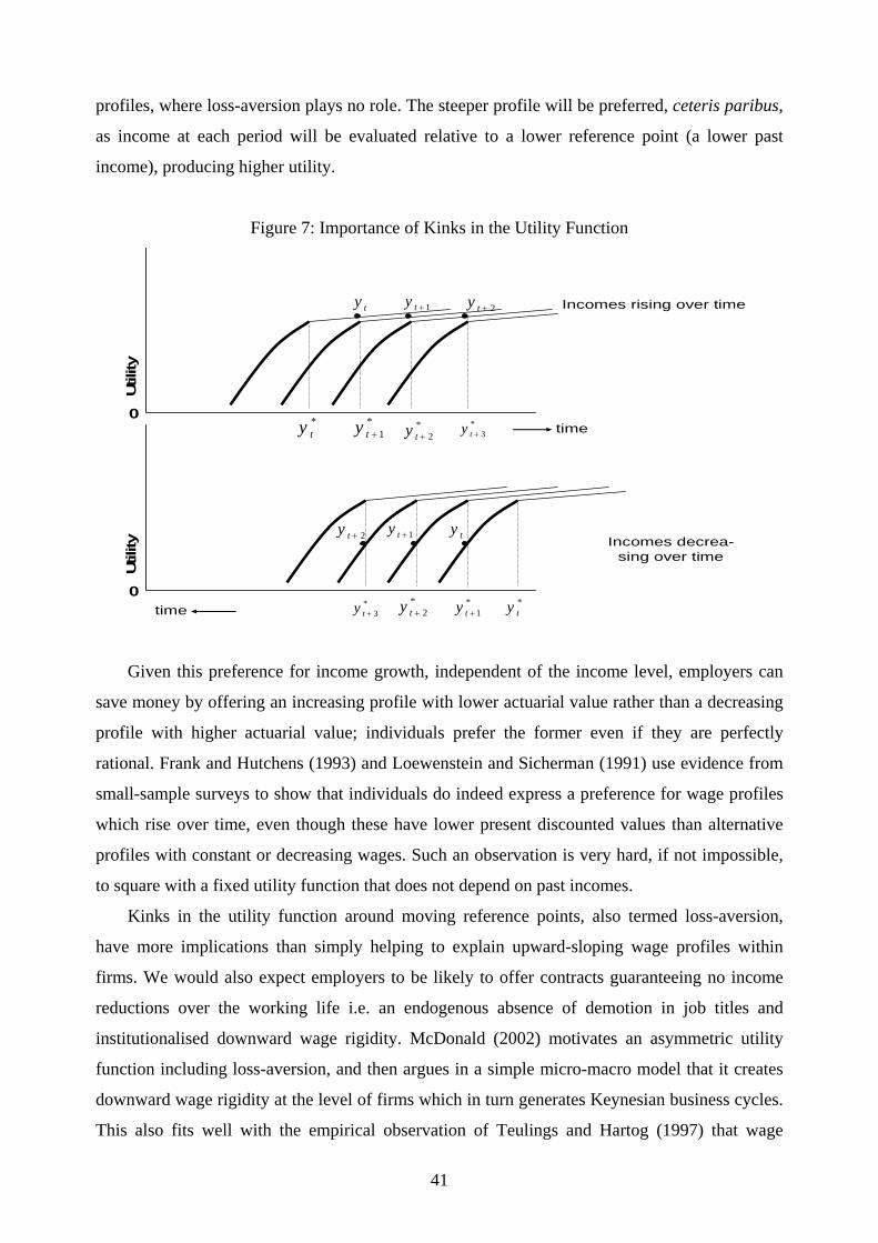
profiles, where loss-aversion plays no role. The steeper profile will be preferred, ceteris paribus,
as income at each period will be evaluated relative to a lower reference point (a lower past
income), producing higher utility.
Figure 7: Importance of Kinks in the Utility Function
0
Util
ity
*ty *
1ty +
Incomes rising over time
*2ty +
ty 1ty + 2ty +
Incomes decrea-sing over time
*3ty + time
0
Util
ity
*ty*
1ty +*
2ty +
ty1ty +2ty +
*3ty +time
Given this preference for income growth, independent of the income level, employers can
save money by offering an increasing profile with lower actuarial value rather than a decreasing
profile with higher actuarial value; individuals prefer the former even if they are perfectly
rational. Frank and Hutchens (1993) and Loewenstein and Sicherman (1991) use evidence from
small-sample surveys to show that individuals do indeed express a preference for wage profiles
which rise over time, even though these have lower present discounted values than alternative
profiles with constant or decreasing wages. Such an observation is very hard, if not impossible,
to square with a fixed utility function that does not depend on past incomes.
Kinks in the utility function around moving reference points, also termed loss-aversion,
have more implications than simply helping to explain upward-sloping wage profiles within
firms. We would also expect employers to be likely to offer contracts guaranteeing no income
reductions over the working life i.e. an endogenous absence of demotion in job titles and
institutionalised downward wage rigidity. McDonald (2002) motivates an asymmetric utility
function including loss-aversion, and then argues in a simple micro-macro model that it creates
downward wage rigidity at the level of firms which in turn generates Keynesian business cycles.
This also fits well with the empirical observation of Teulings and Hartog (1997) that wage
41
decreases are virtually never observed within organisations in Europe because individuals are
sacked rather than demoted. Patacconi and Ederer (2005) also invoke sensitivity to relative
decreases in job status to rationalise the lack of observed empirical reductions in rank and
nominal pay within organisations.
A potentially fruitful avenue for future research along these lines is to test the hypothesis
that retirement partly results from individuals being unwilling to take a step back within their
organisation, and thus choosing retirement over wage cuts or demotion. Retirement would then
generically follow the moment at which individual productivity peaks, even though workers may
still have many highly productive years left. This comes about simply because individuals are
loath to accept jobs and wages that are below their current reference position. In this situation,
there is a case for deferring rewards for production until later in life i.e. to smooth wages such
that they will increase up to some fixed age, which in turn raises the issue of credible long-term
contracts and mandatory retirement.
5.4 Poverty
The relative importance of the three components of the utility function in (1) is crucial for the
measurement of poverty. One common representation is that individuals are in poverty if their
material consumption levels falls below some subsistence level; this appeals to a critical level of
rather than to overall happiness. This approach is behind concepts like the absolute
poverty line, the cost of minimum calorie intake line, and minimum living standards, such as the
minimum consumption basket defining the poverty line in the US, or the 1$ a day poverty line
used by the World Bank. However, Sen (1983) and many others in the poverty literature have
explicitly argued that relative concerns also matter for individuals, and that we should base the
poverty line on relative rather than absolute consumption.33 In this vein, the OECD publishes
statistics on the number of individuals whose income is below half of median income in member
countries, and the European Union currently employs a poverty line set at 60% of median
income. In terms of equation (1), these relative representations of poverty assume that the
component of utility is the most important for individuals. The measurement of
poverty via U2 does however pose problems once we realise that the norm level of income, yt*,
is liable to evolve over time. For instance, if depends on own past income, then, at a given
level of own current income yt, an individual whose income has just increased has higher utility
1 ( )tU c
*2 ( | )t tU y y
*ty
33 One can argue that the concern for relative poverty results from self-interested insurance against negative shocks, and that the lower tail of the income distribution is informative about the size of the negative shocks currently prevalent in the economy.
42
than someone whose income has just decreased, so that poverty depends on both income levels
and income profiles. In practise, taking income adaptation into account for relative poverty
measures would seem to be very difficult.
Neither absolute nor relative poverty lines introduce any explicit role for the non-material
aspects of utility, and are therefore not yet based on happiness. To make the distinction clear
between happiness and whatever we currently mean by poverty, think of a factor like sunshine.
No known definition of poverty considers it to be relevant whether a materially poor person
enjoys more hours of sunshine than a rich person who suffers in a cold climate, even if the
materially poorer person is happier. Implicitly, sunshine and all of the other non-income factors
influencing happiness are considered as orthogonal to poverty, even though they are highly
relevant for both happiness and individual decision-making. Poverty as currently operationalised
concerns the sub-utilities and , instead of happiness proper (U). A more
happiness-based poverty measure would take into account non-material elements to provide a
broader picture of well-being (the lives that individuals live), and would also jar less with the
commonplace observation that individuals freely make a number of choices that leave them
materially worse off (such as having children).
1 ( )tU c *2 ( | )t tU y y
5.5 Optimal taxation and consumption
A burgeoning literature in recent years has addressed the optimal tax implications of utility
functions which depend on relative income; this literature both relies on and produces
predictions about the precise empirical properties of the income-happiness relationship. To our
knowledge, this theoretical literature has not in the past been explicitly connected to the
empirical happiness literature, despite there being clear potential gains from such integration
(Weinzierl, 2005).
One of the most influential papers on optimal taxation is Frank (1985), who adopts the
following utility function:
0 0 1( , ( ), )U U c R c c= (7)
where is the consumption of some positional good, potentially including both positional
material goods (conspicuous consumption) and positional immaterial goods (conspicuous
leisure). This first term of (7) corresponds to in equation (1). The second term in the
utility function,
0c
1 ( )tU c
0( )R c , denotes the individual’s consumption rank with respect to the positional
43
good: this term corresponds broadly to . The third term denotes a non-positional
good and corresponds loosely to
*2 ( |t tU y y )
1 )
1c
3( ,t tU T l Z− . The basic point made by Frank (1985) is that
utility maximisation means that individuals consume up to the point where total marginal
utility is zero:
0c
0 0( ) 0
0 0 0
( ) | |( )
R c cdU dR c dU dU dcdc dc dR c dc dc
+ = − 1
1 0
(8)
where 0( )
0
|R cdUdc
is the marginal utility of the consumption of the positional good keeping rank
constant, 00
0 0
( )|
( )cdR c dU
dc dR c is the marginal utility of the consumption of the positional good via
its effect on rank, and 1
1 0
dU dcdc dc
is the indirect effect of the increased consumption of the
positional good via the (reduced) consumption of the non-positional good. The precise form of
1
0
dcdc
is given by the budget constraint that fixes total income, allowing non-positional goods
to include both leisure and consumption activities. Frank emphasises that
1c
00
0 0
( )|
( )cdR c dU
dc dR c is a
pure externality: changes in rank have no social benefit even though they yield private benefits.
This additional benefit of positional goods to an individual leads to societal over-consumption of
positional goods, to the detriment of non-positional goods. Frank then points out that this
externality produces a rationale for the taxation of the positional good, in order to promote the
non-positional good. If we equate the positional good to relative income and the non-positional
good to leisure, we obtain a rationale for income taxation in order to promote leisure. Layard
(2005) adopts this argument.34
A number of other authors have adopted different specifications of the utility function, and
of the reference position in particular, which affect the tax implications. For example, if we take
the utility function in Ireland (1994):
0 1 0( ( , ), ( ))U U f c c s c= (9)
34 An older literature argues that ‘social preferences’ (also including altruism) can only be identified from observed transfers under restrictive assumptions (direct utility measures do not suffer from this drawback): see Oswald (1983) with respect to taxation and Ng (1987) for the related problem of public good provision.
44
where is a good whose consumption is unobservable, and is status, specified as the
belief spectators have about
1c 0( )s c
0 1( , )f c c based on observing . Exactly as in Frank (1985), Ireland
derives a general tendency to over-consumption of the observable good for a wide class of
possible information regimes. He also illustrates the Pareto improvements that can be attained
via income taxation coupled with direct transfers of to the poor.
0c
0c
1c
Ljungqvist and Uhlig (2000) use a similar utility function, but concentrate on changes in
optimal tax policy over the business cycle. Their main utility function is:
1( ) 1
1t tc c
Uγα
lβγ
−− −= −
− (10)
with tc being the population average of individual consumption , and l denoting labour
supply. This utility function is analogous to that in equation (1), albeit with c and
tc
t tc entered as
separable functions. The externality embedded in the presence of tc leads to labour supply that
is too high, very much in the same mould as Boskin and Sheshinski (1978) and Frank (1985).
Ljungqvist and Uhlig show that this externality can be perfectly countered by a constant
marginal tax on , independent of the business cycle. The analysis is then extended by
considering the reference position not as
tc
tc , but as 1tc − i.e. average consumption last period. In
the presence of aggregate productivity shocks, they find that optimal tax rates co-move with
current productivity shocks, creating counter-cyclical effects of taxation on the economy. This is
exactly in line with the usual Keynesian optimal tax policy which is also counter-cyclical.
5.6 Savings and investment
A related recent theoretical literature has emerged on the dynamic effects of relative
consumption (or status concerns). The papers we mention here abstract from the possibility of a
term like and focus in the main on the timing of consumption. The key question
addressed is the optimality of savings.
3( ,t tU T l Z− 1 )
We might naïvely think that status does not affect savings, because the trade-off between
current and future status would seem to be identical to the trade-off between current and future
consumption. However, this line of thinking breaks down when we consider that individuals
accumulate wealth over their lifetime, and that productivity generally increases, implying that in
45
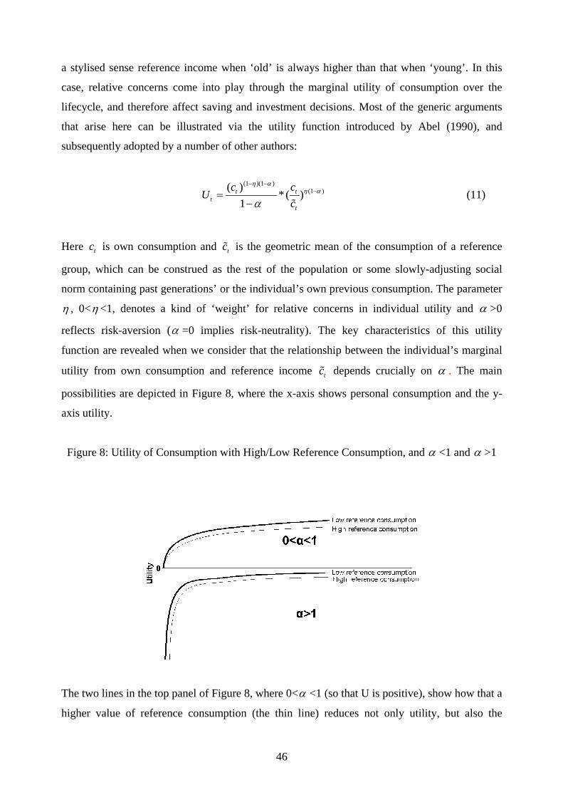
a stylised sense reference income when ‘old’ is always higher than that when ‘young’. In this
case, relative concerns come into play through the marginal utility of consumption over the
lifecycle, and therefore affect saving and investment decisions. Most of the generic arguments
that arise here can be illustrated via the utility function introduced by Abel (1990), and
subsequently adopted by a number of other authors:
(1 )(1 )
(1 )( )* ( )
1t t
tt
c cU
c
η αη α
α
− −−=
− % (11)
Here is own consumption and is the geometric mean of the consumption of a reference
group, which can be construed as the rest of the population or some slowly-adjusting social
norm containing past generations’ or the individual’s own previous consumption. The parameter
tc tc%
η , 0<η <1, denotes a kind of ‘weight’ for relative concerns in individual utility and α >0
reflects risk-aversion (α =0 implies risk-neutrality). The key characteristics of this utility
function are revealed when we consider that the relationship between the individual’s marginal
utility from own consumption and reference income depends crucially on tc% α . The main
possibilities are depicted in Figure 8, where the x-axis shows personal consumption and the y-
axis utility.
Figure 8: Utility of Consumption with High/Low Reference Consumption, and α <1 and α >1
The two lines in the top panel of Figure 8, where 0<α <1 (so that U is positive), show how that a
higher value of reference consumption (the thin line) reduces not only utility, but also the
46
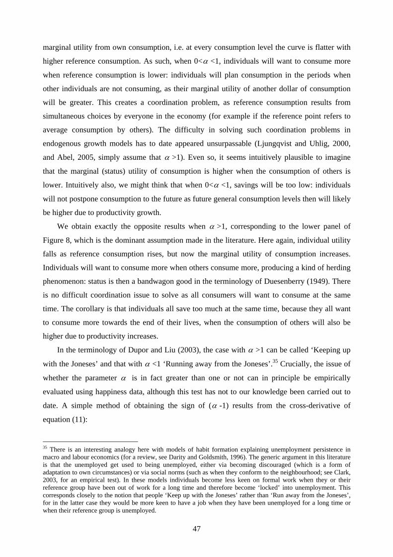
marginal utility from own consumption, i.e. at every consumption level the curve is flatter with
higher reference consumption. As such, when 0<α <1, individuals will want to consume more
when reference consumption is lower: individuals will plan consumption in the periods when
other individuals are not consuming, as their marginal utility of another dollar of consumption
will be greater. This creates a coordination problem, as reference consumption results from
simultaneous choices by everyone in the economy (for example if the reference point refers to
average consumption by others). The difficulty in solving such coordination problems in
endogenous growth models has to date appeared unsurpassable (Ljungqvist and Uhlig, 2000,
and Abel, 2005, simply assume that α >1). Even so, it seems intuitively plausible to imagine
that the marginal (status) utility of consumption is higher when the consumption of others is
lower. Intuitively also, we might think that when 0<α <1, savings will be too low: individuals
will not postpone consumption to the future as future general consumption levels then will likely
be higher due to productivity growth.
We obtain exactly the opposite results when α >1, corresponding to the lower panel of
Figure 8, which is the dominant assumption made in the literature. Here again, individual utility
falls as reference consumption rises, but now the marginal utility of consumption increases.
Individuals will want to consume more when others consume more, producing a kind of herding
phenomenon: status is then a bandwagon good in the terminology of Duesenberry (1949). There
is no difficult coordination issue to solve as all consumers will want to consume at the same
time. The corollary is that individuals all save too much at the same time, because they all want
to consume more towards the end of their lives, when the consumption of others will also be
higher due to productivity increases.
In the terminology of Dupor and Liu (2003), the case with α >1 can be called ‘Keeping up
with the Joneses’ and that with α <1 ‘Running away from the Joneses’.35 Crucially, the issue of
whether the parameter α is in fact greater than one or not can in principle be empirically
evaluated using happiness data, although this test has not to our knowledge been carried out to
date. A simple method of obtaining the sign of (α -1) results from the cross-derivative of
equation (11):
35 There is an interesting analogy here with models of habit formation explaining unemployment persistence in macro and labour economics (for a review, see Darity and Goldsmith, 1996). The generic argument in this literature is that the unemployed get used to being unemployed, either via becoming discouraged (which is a form of adaptation to own circumstances) or via social norms (such as when they conform to the neighbourhood; see Clark, 2003, for an empirical test). In these models individuals become less keen on formal work when they or their reference group have been out of work for a long time and therefore become ‘locked’ into unemployment. This corresponds closely to the notion that people ‘Keep up with the Joneses’ rather than ‘Run away from the Joneses’, for in the latter case they would be more keen to have a job when they have been unemployed for a long time or when their reference group is unemployed.
47
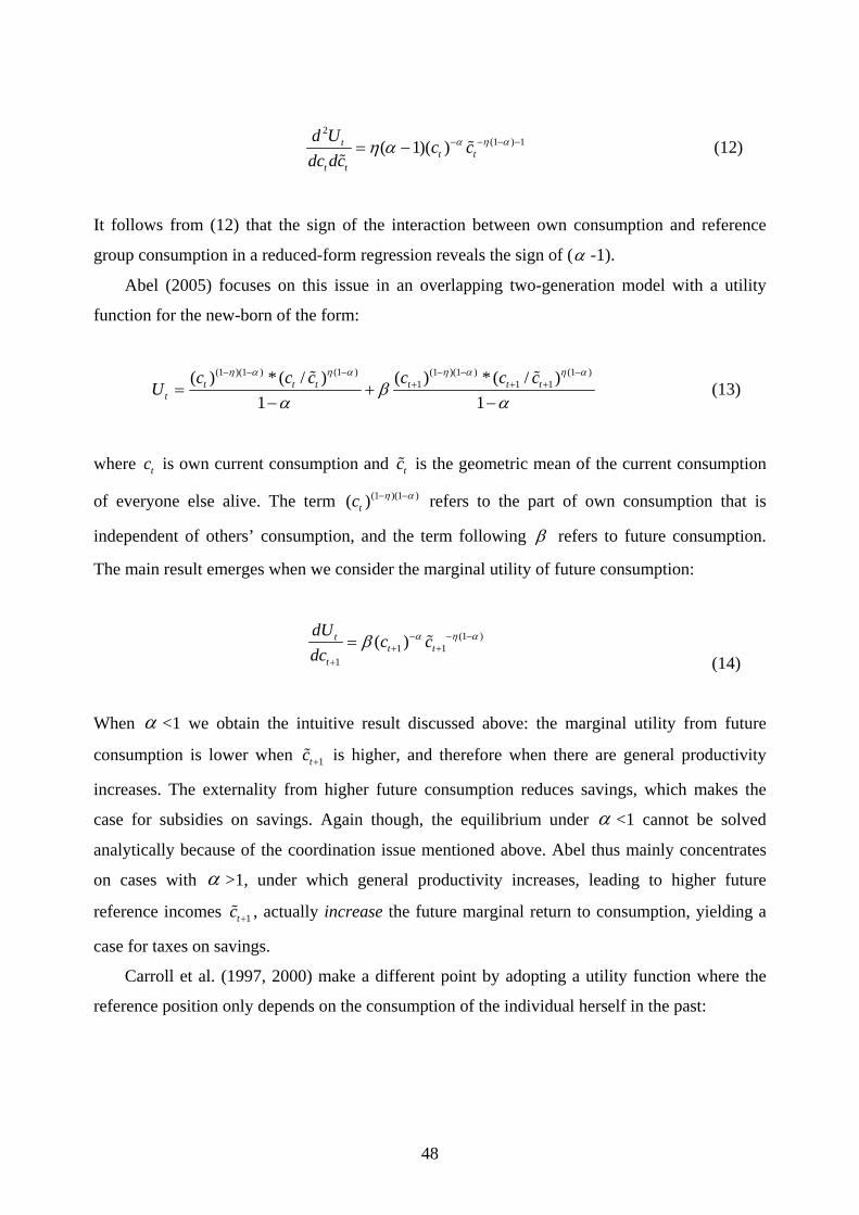
2
(1 ) 1( 1)( )tt t
t t
d Uc c
dc dcα η αη α − − − −= − %
% (12)
It follows from (12) that the sign of the interaction between own consumption and reference
group consumption in a reduced-form regression reveals the sign of (α -1).
Abel (2005) focuses on this issue in an overlapping two-generation model with a utility
function for the new-born of the form:
(1 )(1 ) (1 ) (1 )(1 ) (1 )
1 1 1( ) * ( / ) ( ) * ( / )1 1
t t t t t tt
c c c c c cU
η α η α η α η
βα α
− − − − − −+ + += +
− −% α%
(13)
where is own current consumption and is the geometric mean of the current consumption
of everyone else alive. The term
tc tc%
(1 )(1 )( )tc η α− − refers to the part of own consumption that is
independent of others’ consumption, and the term following β refers to future consumption.
The main result emerges when we consider the marginal utility of future consumption:
(1 )1 1
1
( )tt t
t
dUc c
dcα η αβ − − −
+ ++
= %
(14)
When α <1 we obtain the intuitive result discussed above: the marginal utility from future
consumption is lower when is higher, and therefore when there are general productivity
increases. The externality from higher future consumption reduces savings, which makes the
case for subsidies on savings. Again though, the equilibrium under
1tc +%
α <1 cannot be solved
analytically because of the coordination issue mentioned above. Abel thus mainly concentrates
on cases with α >1, under which general productivity increases, leading to higher future
reference incomes , actually increase the future marginal return to consumption, yielding a
case for taxes on savings.
1tc +%
Carroll et al. (1997, 2000) make a different point by adopting a utility function where the
reference position only depends on the consumption of the individual herself in the past:
48
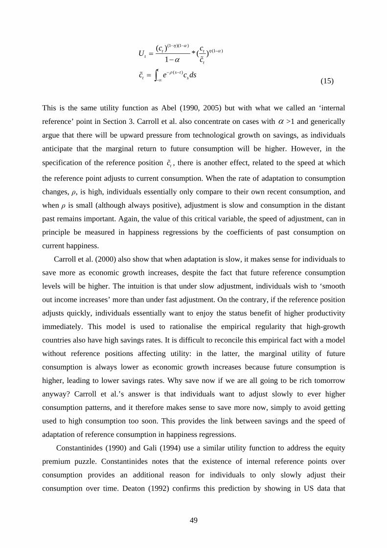
(1 )(1 )(1 )
( )
( )* ( )
1t t
tt
t s tt s
c cU
c
c e c ds
η αη α
ρ
α
− −−
− −
−∞
=−
= ∫
%
% (15)
This is the same utility function as Abel (1990, 2005) but with what we called an ‘internal
reference’ point in Section 3. Carroll et al. also concentrate on cases with α >1 and generically
argue that there will be upward pressure from technological growth on savings, as individuals
anticipate that the marginal return to future consumption will be higher. However, in the
specification of the reference position , there is another effect, related to the speed at which
the reference point adjusts to current consumption. When the rate of adaptation to consumption
changes, ρ, is high, individuals essentially only compare to their own recent consumption, and
when ρ is small (although always positive), adjustment is slow and consumption in the distant
past remains important. Again, the value of this critical variable, the speed of adjustment, can in
principle be measured in happiness regressions by the coefficients of past consumption on
current happiness.
tc%
Carroll et al. (2000) also show that when adaptation is slow, it makes sense for individuals to
save more as economic growth increases, despite the fact that future reference consumption
levels will be higher. The intuition is that under slow adjustment, individuals wish to ‘smooth
out income increases’ more than under fast adjustment. On the contrary, if the reference position
adjusts quickly, individuals essentially want to enjoy the status benefit of higher productivity
immediately. This model is used to rationalise the empirical regularity that high-growth
countries also have high savings rates. It is difficult to reconcile this empirical fact with a model
without reference positions affecting utility: in the latter, the marginal utility of future
consumption is always lower as economic growth increases because future consumption is
higher, leading to lower savings rates. Why save now if we are all going to be rich tomorrow
anyway? Carroll et al.’s answer is that individuals want to adjust slowly to ever higher
consumption patterns, and it therefore makes sense to save more now, simply to avoid getting
used to high consumption too soon. This provides the link between savings and the speed of
adaptation of reference consumption in happiness regressions.
Constantinides (1990) and Gali (1994) use a similar utility function to address the equity
premium puzzle. Constantinides notes that the existence of internal reference points over
consumption provides an additional reason for individuals to only slowly adjust their
consumption over time. Deaton (1992) confirms this prediction by showing in US data that
49
individuals over-smooth consumption after permanent income shocks. Constantinides goes
further by arguing that the presence of creates a bias in conventional estimates of risk-
aversion, which are based on the tradeoffs people make over time: without then high risk-
aversion would imply that the savings rates of the rich would be greater than those of the poor.
The fact that savings rates vary only little across income groups may lead us to conclude that
risk-aversion is actually quite low. Constantinides shows that the presence of breaks this
logic, in that even with high risk-aversion the presence of a moving reference point leads all
individuals to smooth income over time in a similar manner. This provides a rationale for
empirical instances of observed high instantaneous risk-aversion, in particular the large premium
that individuals are prepared to pay for risk-free assets versus risky higher-return assets i.e. the
equity premium puzzle. Campbell and Cochrane (1999) extend this idea to further types of asset
pricing puzzles and argue that models including a reference point exhibit superior predictive
power over models without such a term.
tc%
tc%
tc%
tc%
Reference point models have also been used to explain financial contagion where reference
effects are usually termed ‘habit formation’. The main observation that this literature addresses
is the Asian financial crisis, whereby a whole set of countries saw their exchange rates and
economies collapse in sequence (see for a description Eichengreen et al., 2001). A puzzling
feature for more standard models is that during the Asian financial crisis the risk premia for
holding a financial asset went up in all of the countries involved when the currency of another
country collapsed, whereas in standard theories one would expect capital flight from the affected
country to the other countries which would reduce risk premia. Boschi and Goenka (2006), who
adopt the utility function of Cambell and Cochrane (1999) which is very similar to Abel’s
(1990) specification, argue that this increase in risk premia may be due to the fact that if own
wealth comes close to the reference wealth level (due to losses incurred in another country) the
curvature of the utility function increases. The greater the curvature of the utility function, the
more compensation investors needs to keep investing in a country, meaning that the risk premia
go up which in turn may lead to the collapse of a currency. This general idea can also be seen in
Figure 8: the ‘steepness’ reduces faster when reference incomes are relatively high relative to
own income and thus risk aversion is stronger. The same principle applies with wealth if
individuals realise that making a loss on current wealth may reduce consumption below
reference consumption. Whilst Boschi and Goenka (2006) claim such increases in risk premia
due to wealth effects cannot be explained by standard (CARA) utility functions, it may of course
be the case that financial contagion works via channels other than wealth effects in combination
50
with habit formation. We could for instance alternatively argue that the collapse of one country
is informative about ‘fundamentals’ in a similar country. This is therefore a good example of a
situation where reference group effects may explain an observable outcome but where it is hard
to dismiss other possibilities that do not involve reference groups; there are indeed dozens of
other competing theories (see the lengthy discussion in Boschi and Goenka, 2006). This
underlines the importance of laboratory evidence on the influence of reference groups for this
literature, since only then can we be sure that there are no other factors involved and that
reference groups really do have independent effects on choice behaviour.
One particular strand of the empirical income-happiness literature fits in well with savings
models, namely the so-called ‘tunnel-effect’. The original idea is attributed to Hirschman
(1973), who argued that individuals could actually derive utility from others’ higher incomes if
they consider them to be informative about their own future income. Senik (2004) uses this
argument to explain why in Russian panel data (RLMS) individual happiness was positively
linked to reference group income, rather than negatively as a relative utility function would
suggest. Equally, Senik (2005) finds that higher reference group income reduces life satisfaction
in Western Europe, but raises life satisfaction in the post-Transition countries of Eastern Europe
(and the United States). The potential importance of the information role is underscored by the
finding that reference group income is more strongly positively correlated with life satisfaction
for those in more uncertain situations (as measured by the volatility of their income and the
probability of losing their job, for example).
The simplest model in which a tunnel effect can arise is a two-period model where
individuals only derive utility from their own consumption, but face the problem of saving in
period 1 in order to consume in period 2. For example, consider:
1 2
2 21 1
11 2
2
( ) ( )
1 1
'( ) (1 ) '( ) 0
U u c u cc yc y
r rdcu c r u cdy
= +
+ = ++ +
→ = + → >
(16)
where lifetime utility U is now simply the sum of happiness in period 1, which depends only on
period 1 consumption, and happiness in period 2, which depends only on period 2 consumption.
The budget constraint (with an interest rate of r) links period 1 consumption to period 2 income:
the higher is period 2 income, the higher is period 1 consumption because of a reduced need for
savings. Now imagine that period 2 income is in fact unknown by the individual decision-maker,
51
who estimates her next-period income from the incomes of ‘reference’ individuals around her
who share the same observable characteristics (region, education, gender, age, etc.). This
produces a reduced-form lifetime happiness function in the first period that depends positively
on the observed incomes of reference individuals. Neither adaptation nor social comparisons are
needed to produce a relationship between happiness and others’ income; although equally, under
certain parameterisations, tunnel effects can be observed even if relative income or consumption
matters.
The tunnel-effect model provides several pointers as to what we should expect to observe
empirically: (i) we should see a positive relationship between reference group income and own
current consumption, over and above the effect of own income (because the higher is others’
income, the lower are one’s own savings); and (ii) we should observe happiness being positively
correlated with reported expected future income, and that the positive effect of reference group
income on one’s own happiness transits via expected future income. These tunnel-effect
predictions are yet to be empirically tested.
5.7 Migration
Consider the decision whether to migrate or not. Without a term in the utility
function, then all those who find more attractive income and leisure combinations in another
country will leave. This conclusion changes if we allow for comparisons, and consider that
migration might lead to changes in . For instance, if equals average income in the local
neighbourhood or the average income of people like yourself at your workplace, then someone
who fears ending up with low relative income in another country might not migrate, even if both
leisure and the absolute income she could earn there are higher. Stark and Taylor (1991) appeal
to this idea to explain why the elites in poor countries do not emigrate: the elite are at the top of
the income distribution in the country where they currently live, but may well not be so if they
emigrate. Stark and Taylor further introduce the notion of different economic migrant types. In
terms of equation (1), they argue that we would expect those with relatively high earnings
potential in another country to move abroad e.g. those whose skills are relatively undervalued in
the country of origin. Furthermore, we expect those who can keep individuals in their home
(poorer) country as their reference group to be more likely to emigrate than those whose
reference income adapts to the new country. The former can become high-status in their home
country by earning more in the host country, yet they remain in a status sense part of the home
country. This line of thinking can help to explain why many migrants continue to visit their
home country: this is when they can cash in as relatively high earners compared to those in the
*2 ( | )t tU y y
*ty *
ty
52
home country, making it irrelevant whether those same incomes are considered as high in the
host country.36
This kind of analysis yields two distinct possible migration dynamics. In the first, those who
migrate do so voluntarily in spite of adaptation in the element of their utility
function. That is, they have exceptionally high skills and can become high-status even in the
host country and want to compare themselves to persons in the host country anyway. The first
group of voluntary migrants is therefore made up of high-status assimilators, who Stark
identifies with the brain-drain phenomenon. The networks of these early migrants may lead to
more migration of the same variety, but the fast assimilation of early migrants implies that they
are not preoccupied by this, as their networks will not primarily consist of other migrants from
the same home country. The second migration pattern is very different, and may well result from
exceptionally low consumption in the home country (i.e. by ). For example, we can think
of the Irish in the US being driven by the potato famine back home, forced migration in general,
or the ‘guest worker phenomenon’ of the European Union where whole villages were essentially
transplanted to other countries in the 1960’s. These individuals will by design be less likely to
assimilate, and have strong incentives to carry on comparing themselves to individuals in the
home country. This results from their high wages relative to those in the home country and low
wages relative to the host country. These migrants may for the same reason try to attract more
low-skill individuals from the home country, as these latter do not detract from their own status
but rather increase it by reducing the reference income they face in the host country. The two
types of immigration, associated with two different parts of the income/happiness gradient, will
therefore have very different cultural and economic implications for the host country. Countries
such as Canada and Australia, which operate a points system whereby potential migrants have to
offer something exceptional to the host country in order to attain a visa, arguably attempt to
attract the first type of economic migrant. Countries in the EU that are introducing legislation
trying to stop ‘family reunions’ could be interpreted as trying to reduce the second kind of
economic migrant. More empirical work on the relationship between happiness and reference
*2 ( |t tU y y )
1 ( )tU c
36 It could be argued that the same observation could be rationalised by a standard utility function without relativity in a situation where prices are low in the home country, but wages are high in the host country. Migrants going home for the holidays would then simply be taking advantage of the higher purchasing power of their income in the home country. That would then, however, beg the question as to why the non-migrants of that host country do not also visit the ‘home’ country in large numbers. If it is really an issue of prices, there would be no inherent reason for migrants to return to their home country: they could equally go to any other low-price country. We can, of course, object to this line of thinking by saying that migrants return to their home country because of specific ties with family or others that further lowers the price of some goods for them. It is possible to derive alternative rationalisations of return migration that do not depend on relative considerations.
53
incomes, especially looking at the differences across migrant groups in reference incomes,
would greatly inform this debate.
5.8 Normative Implications
Section 5.5 discussed the tax implications of relative utility. These arise due to externalities
between individuals. Somewhat more subtle are the policy implications of adaptation, which can
be thought of as externalities within individuals. We discussed above how changing reference
incomes can affect inter-temporal trade-offs in consumption, wage profiles, and the costs and
benefits of migration. In general, events to which individuals adapt quickly only have a
happiness payoff in the short run, while events where adaptation is slow (or absent), have long-
run happiness payoffs. The impact of a particular circumstance on current happiness is then only
a snapshot of the stream of effects on happiness associated with that circumstance, and is
therefore in principle not necessarily informative about life-time trade-offs.
What is often not well-understood is that as long as individuals are rational, the mere
presence of adaptation is no reason for policy intervention unless it is accompanied by an
externality (such as those found in social comparisons). We may not necessarily want to
counteract activities which produce only a short-lived happiness ‘buzz’ at the expense of a long-
run happiness cost, unless we believe that individuals are unaware of the fact that the ‘buzz’ may
indeed only be ephemeral.
When individuals do not in fact realise that they will get used to some things (but not to
others), a basic paternalistic question arises. This has been well-stated by many, including
Kahneman et al. (1997, 1999) and Rabin (1998): Should we only care about what Self 0 (who
makes the decisions) wants or should we also care about what Self 1 (in the future) experiences?
Individuals who care only about their desires at time 0 (i.e. Self 0) will take decision utility as
the normative reference point. If instead we were to take the experiences of Self 1 as the guiding
principle for policy design, we would potentially act against the explicit wishes of an ‘ignorant’
(Self 0) electorate by taxing activities that lead to only short-run happiness gains. An interesting
political economy question then arises of how governments can do so without being voted out of
office by myopic Self 0’s. This question only arises when individuals mis-forecast their degree
of adaptation. However, the empirical literature is still only beginning to grapple with the
questions of differential paces of adaptation to life events. While there is now growing evidence
regarding the misprediction of adaptation (see Riis et al., 2005, and the research reviewed in
Loewenstein and Ubel, 2006), the information required to advocate paternalism is currently far
from complete.
54
6. Conclusions
One of the exciting developments within economics over the last decade has been the booming
‘economics of happiness’ literature, which has expanded in both theoretical and empirical
directions. The basis for the empirical work has been the increasing evidence from both
psychologists and economists that measures of individual well-being collected in surveys
contain ‘valid variability’, in the sense that current happiness or satisfaction is a strong predictor
of future behaviour. The wider acceptance of subjective well-being measures as a direct proxy
for utility has consequently opened up a wide-range of opportunities to further inform theory
and policy design. The happiness literature has in the last few years began to make major
inroads in this respect. The analysis of subjective well-being data provides a valuable
alternative, but complementary, approach to the revealed-preference framework that dominates
the discipline of economics.
The two specific issues that have generated the most interest in the literature are (i) the
effect of labour market status, and especially unemployment, on happiness, and (ii) the
relationship between income and happiness. This paper has focussed on the latter, motivated by
its central importance to economists and policy-makers. Our contribution has been to provide a
new overview of the theoretical and empirical literature on income and happiness, bringing
together the most recent research, and showing how the traditional utility function framework
can be readily generalised to incorporate a range of observed behaviours. In particular, our main
challenge has been to align the widely-cited Easterlin ‘Paradox’, that of increasing real incomes
in developed countries but with no noticeable increase in average happiness, with the large
empirical survey literature that has found that income and happiness are positively related.
The broad consensus in the literature is that the paradox points to the importance of relative
considerations in the utility function, where higher income brings both consumption and status
benefits to an individual. Comparisons can either be to others or to oneself in the past. Utility
functions of this type can explain the positive slope found in much of the empirical literature.
However, since status is a zero-sum game, only the consumption benefit of income remains at
the aggregate level. Since the consumption benefit approaches zero as income rises, happiness
profiles over time in developed countries are flat. Carlyle’s pitifulest whipster will indeed be
made happier by higher income, but only at the expense of someone else or his own future self.
We have appealed to the growing literature to show that happiness is indeed negatively
related to others’ incomes and to own past income. We are aware though that it will never be
possible to prove that happiness measures utility. We thus also discuss the reasons why we
55
believe the two are related, and review evidence consistent with relative utility from non-
happiness sources.
Going beyond the paradox that initiated the literature, this paper has attempted to connect the
economics of happiness literature with theoretical economic models of taxation, labour supply,
economic growth, savings, wage profiles, migration, and consumption. We have identified how
the outcomes of mainstream theoretical models hinge on key behavioural parameters that could
in principle be identified from the empirical analysis of happiness data. Some examples of these
parameters include:
i. The degree of risk-aversion and the complementarity between own income and
reference income, which are important for the savings literature;
ii. The malleability of reference groups, which is key to migration decisions and
education decisions;
iii. The kink in utility functions around the reference position, which is important for
wage policies and career decisions; and,
iv. The existence and extent of material and non-material status races, which are
paramount for optimal taxation policy.
The interaction between economic theory and happiness is therefore the next milestone for
the developing economics of happiness literature. However, it is clear that the empirical
literature on happiness still faces several challenges, many of which are shared with other
empirical literatures. Two of the key challenges are to deal with a general inability of survey
data to precisely time changes in income with changes in happiness over long time periods, and
the difficulty in mapping incomes into current and expected consumption. It is also the case that
most datasets do not contain reliable (if any) ex ante information regarding the group (the
reference point) to which individuals compare themselves. Similarly, no dataset can contain all
the variables of importance, so that researchers will continue to face the issue of endogeneity
with respect to income and other variables such as marriage, education, and the reference group.
Finally, natural experiments producing exogenous variation in income are only rarely observed,
making the issue of establishing the causal effect of income on happiness a major challenge.
Our final conclusion is that taking relative income seriously is an important step towards
greater behavioural realism in Economics, such that our models and empirical analysis move
closer to how real people feel and behave. Some may not like the insertion of additional
arguments into individual utility, and remark that any behaviour can be rationalised by an
56
appropriate manipulation of the utility function. While this is formally true, it does not apply
wholesale to the issue of relative income. As we have tried to demonstrate, utility functions
including relative income terms produce a wide variety of testable predictions regarding both
well-being (measured by survey or neurologically) and observable behaviours: it is not true that
“anything goes”. To our mind, this is precisely why we need to appeal to both direct measures of
utility and observed behaviour in order to obtain a better idea of what the utility function looks
like, and make policy recommendations in the best interest of society. Testing these predictions
not only allies theory and empirical analysis in economics, it also spills across many disciplines
in the social and natural sciences; it is arguably the most important and the most promising of
the research avenues open to this thriving literature.
References Abel, A.B. (1990). Asset prices under habit formation and catching up with the Joneses.
American Economic Review, vol. 80, pp. 38-42. Abel, A.B. (2005). Optimal taxation when consumers have endogenous benchmark levels of
consumption. Review of Economic Studies, vol. 72, pp. 21-42. Alesina, A., Di Tella, R, and MacCulloch, R. (2004). Inequality and happiness: Are Europeans
and Americans different? Journal of Public Economics, vol. 88, pp. 2009–2042. Alpizar, F., Carlsson, F. and Johansson-Stenman, O. (2005). How much do we care about
Absolute versus relative income and consumption? Journal of Economic Behavior and Organization, vol. 56, pp. 405-421.
Angner, E. (2005). The evolution of Eupathics: The historical roots of subjective measures of well-being. University of Alabama at Birmingham, mimeo.
Barker, D. (2005). The developmental origins of well-being. In F. Huppert, N. Baylis and B. Keverne (Eds.), The science of well-being. Oxford: Oxford University Press.
Bertrand, M. and Mullainathan, S. (2001). Do people mean what they say? Implications for subjective survey data. American Economic Review, vol. 91, pp. 67-72.
Blanchflower, D.G. and Oswald, A.J. (2004). Well-being over time in Britain and the USA. Journal of Public Economics, vol. 88, pp. 1359-1386.
Boes, S., Lipp, M. and Winkelmann, R. (2007). Money illusion under test. Economics Letters, vol. 94, pp. 332-337.
Boschi, M. and Goenka, A. (2006). Habit formation and the transmission of financial crises. Working Paper 608, University of Essex.
Boskin, M. and Sheshinski, E. (1978). Optimal redistributive taxation when individual welfare depends upon relative income. Quarterly Journal of Economics, vol. 92, pp. 589-601.
Brickman, P.C.D. and Campbell, D. (1971). Hedonic relativism and planning the good society. In M. H. Appley (ed.), Adaptation-Level Theory: A Symposium. New York. Academic Press.
Brickman, P.C.D., Coates, D. and Janoff-Bulman, R. (1978). Lottery winners and accident victims: Is happiness relative? Journal of Personality and Social Psychology, vol. 36, pp. 917-927.
Blanchflower, D.G. and Oswald, A.J. (2007). Hypertension and Happiness across Nations, University of Warwick, mimeo.
Brosnan, S. and De Waal, F. (2003). Monkeys reject unequal pay. Nature, vol. 425, pp. 297-299.
57
Brown, G., Gardner, J., Oswald, A.J. and Qian, J. (2006). Does wage rank affect employees' wellbeing? University of Warwick, mimeo.
Burchardt, T. (2005). Are one man's rags another man's riches? Identifying adaptive preferences using panel data. Social Indicators Research, vol. 74, pp. 57-102.
Campbell, J.Y. and Cochrane, J.H. (1999). By force of habit: A consumption-based explanation of aggregate stock market behaviour. Journal of Political Economy, vol. 107, pp. 205-251.
Cappelli, P. and Sherer, P.D. (1988). Satisfaction, market wages and labour relations: An airline study. Industrial Relations, vol. 27, pp. 56-73.
Carroll, N, Frijters, P., and Shields, M.A. (2007). Quantifying the costs of drought: New evidence from life satisfaction data. Journal of Population Economics, forthcoming.
Carroll, C., Overland, J. and Weil, D.N. (1997). Comparison utility in a growth model. Journal of Economic Growth, vol. 2, pp. 339-67.
Carroll, C.D., Overland, J. and Weil, D.N. (2000). Saving and growth with habit formation. American Economic Review, vol. 90, pp. 341-55.
Chen, M, Lakshminarayanan, V. and Santos, L. (2006). How Basic Are Behavioral Biases? Evidence from Capuchin Monkey Trading Behavior. Journal of Political Economy, vol. 114, pp. 517-537.
Cherkas, L., Aviv, A., Valdes, A., Hunkin, J., Gardner, J., Surdulescu, G., Kimura, M. and Spector, T. (2006). The effects of social status on biological aging as measured by white-blood-cell telomere length. Aging Cell, vol. 5, pp. 361-365.
Clark, A.E. (1996a). L'utilité est-elle relative? Analyse à l'aide de données sur les ménages. Economie et Prévision, vol.121, pp. 151-164.
Clark, A. E. (1996b). Job Satisfaction in Britain. British Journal of Industrial Relations, vol. 34, pp. 189-217.
Clark, A.E. (1997). Job satisfaction and gender: Why are women so happy at work? Labour Economics, vol. 4, pp. 341-372.
Clark, A.E. (1999). Are wages habit-forming? Evidence from micro data. Journal of Economic Behavior and Organization, vol. 39, pp. 179-200.
Clark, A.E. (2001). What really matters in a Job? Hedonic measurement using quit data. Labour Economics, vol. 8, pp. 223-242.
Clark, A.E. (2003). Unemployment as a social norm: Psychological evidence from panel data. Journal of Labor Economics, vol. 21, pp. 323-351.
Clark, A.E., Etilé, F., Postel-Vinay, F., Senik, C. and Van der Straeten, K. (2005). Heterogeneity in reported well-being: Evidence from twelve European countries. Economic Journal, vol. 115, pp. C118-C132.
Clark, A.E., Georgellis, Y. and Sanfey, P. (1998). Job satisfaction, wage changes and quits: Evidence from Germany. Research in Labor Economics, vol. 17, pp. 95-121.
Clark, A.E., Georgellis, Y. and Sanfey, P. (2001). Scarring: The psychological impact of past unemployment. Economica, vol. 68, pp. 221-241.
Clark, A.E., Masclet, D. and Villeval, M.C. (2006). Effort and comparison income. IZA Discussion Paper No. 2169, Bonn.
Clark, A.E. and Oswald, A.J. (1996). Satisfaction and comparison income. Journal of Public Economics, vol. 61, pp. 359-81.
Cohen, S., Doyle, W., Turner, R., Alper, C. and Skoner, D. (2003). Emotional style and susceptibility to the common cold. Psychosomatic Medicine, vol. 65, pp. 652-657.
Constantinides, G.M. (1990). Habit formation: A resolution of the equity premium puzzle. Journal of Political Economy, vol. 98, pp. 519-43.
Corneo, G. and Jeanne, O. (2001). Status, the distribution of wealth, and growth. Scandinavian Journal of Economics, vol. 103, pp. 283-293.
58
Cromwell, H., Hassani, O. and Schultz, W. (2005). Relative reward processing in primate striatum. Experimental Brain Research, vol. 162, pp. 520–525.
Daly, M. and Wilson, D. (2005). Keeping up with the Joneses and staying ahead of the Smiths. Evidence from suicide data. Federal Reserve Bank of San Francisco, Working Paper no. 2006-12.
Darity, W. and Goldsmith, A.H. (1996). Social psychology, unemployment and macroeconomics. Journal of Economic Perspectives, vol. 10, pp. 121-140.
Davidson R.J. (2004). Well-being and affective style: neural substrates and biobehavioural correlates. Philosophical Transactions of the Royal Society (London), vol. 359, pp. 1395-411
Deaton, A. (1992). Understanding Consumption. Oxford: Clarendon Press. Deci, E. and Ryan, R. (2000). The "what" and "why" of goal pursuits: Human needs and the
self-determination of behaviour. Psychological Inquiry, vol. 11, pp. 227-268. Di Tella, R. and MacCulloch, R. (2005a). Gross National Happiness as an answer to the
Easterlin Paradox? Harvard Business School, mimeo. Di Tella, R. and MacCulloch, R. (2006). Some uses of happiness data in economics. Journal of
Economic Perspectives, vol. 20, pp. 25-46. Di Tella, R., MacCulloch, R. and Haisken-DeNew, J.P. (2005). Happiness adaptation to income
and to status in an individual panel. Harvard Business School Working Paper. Di Tella, R. MacCulloch, R. and Oswald, A.J. (2003). The macroeconomics of happiness.
Review of Economics and Statistics, vol. 85, pp. 809–827. Diener, E., Diener, M. and Diener, C. (1995). Factors predicting the subjective well- being of
nations. Journal of Personality and Social Psychology, vol. 69, pp. 851-864. Diener, E. and Lucas, R.E. (1999). Personality and subjective well-being. In Kahneman, D.,
Diener, E. and Schwarz, N. (Eds), Foundations of Hedonic Psychology: Scientific Perspectives on Enjoyment and Suffering, Chapter 11. New York: Russell Sage Foundation.
Duesenberry, J.S. (1949). Income, Saving and the Theory of Consumer Behavior. Cambridge, MA, Harvard University Press.
Dupor B. and Liu W.F. (2003). Jealousy and equilibrium overconsumption. American Economic Review, vol. 93, pp. 423-428.
Easterlin, R. (1974). Does economic growth improve the human lot? Some empirical evidence. In David, R. and Reder, R. (Eds.), Nations and Households in Economic Growth: Essays in Honor of Moses Abramovitz. New York: Academic Press.
Easterlin, R.A. (1995). Will raising the incomes of all increase the happiness of all? Journal of Economic Behavior and Organization, vol. 27, pp. 35-47.
Easterlin, R.A. (2001). Income and happiness: Towards a unified theory. Economic Journal, vol. 111, pp. 465-484.
Easterlin, R.A. (2005a). Feeding the illusion of growth and happiness: A reply to Hagerty and Veenhoven. Social Indicators Research, vol. 74, pp. 429-443.
Easterlin, R.A. (2005b). A puzzle for adaptive theory. Journal of Economic Behavior and Organization, vol. 56, pp. 513-521.
Eichengreen, B., Hale, G., and Mody, A. (2001). Flight to quality: investor risk tolerance and the spread of emerging market crises. In International Financial Contagion, S. Claessens and K. Forbes (eds.), Kluwer USA.
Elster, J. and Roemer, J. (1993, Eds.). Interpersonal Comparisons of Well-Being. Cambridge University Press.
Falk, A. and Knell, M. (2004). Choosing the Joneses: Endogenous goals and reference standards. Scandinavian Journal of Economics, vol. 106, pp. 417-435.
Fernández-Dols, J. and Ruiz-Belda, M. (1995). Expression of emotion versus expressions of emotions: Everyday conceptions about spontaneous facial behavior. In Russell, J., Fernández-
59
Dols, J., Manstead, A. and Wellenkamp, J. (Eds.), Everyday conceptions of emotion. Dordrecht: Kluwer.
Ferrer-i-Carbonell, A. (2005). Income and well-being: An empirical analysis of the comparison income effect. Journal of Public Economics, vol. 89, pp. 997-1019.
Ferrer-i-Carbonell, A. and Frijters, P. (2004). How important is methodology for the estimates of the determinants of happiness? Economic Journal, vol. 114, pp. 641-659.
Fershtman, C., Murphy, K.M. and Weiss, Y. (1996). Social status, education, and growth. Journal of Political Economy, vol. 104, pp. 108-132
Fließbach K., Weber B, Trautner P., Dohmen T., Sunde U., Elger C., and Falk A. (2007), Social comparison affects reward-related brain activity in the human ventral striatum, University of Bonn, mimeo.
Frank, R.H. (1985). Choosing the Right Pond. Oxford: Oxford University Press. Frank, R.H. (1999). Luxury Fever . New York: The Free Press. Frank, R.H. and Hutchens, R.M. (1993). Wages, seniority, and the demand for rising
consumption profiles. Journal of Economic Behavior and Organization, vol. 21, pp. 251-276. Frederick, S. and Loewenstein, G. (1999). Hedonic adaptation. In Kahneman, D., Diener, E. and
Schwarz, N. (Eds), Foundations of Hedonic Psychology: Scientific Perspectives on Enjoyment and Suffering, Chapter 16. New York: Russell Sage Foundation.
Freeman, R. (1978). Job satisfaction as an economic variable. American Economic Review, vol. 68, pp. 135-141.
Frey, B.S. and Stutzer, A. (2002a). What can economists learn from happiness research? Journal of Economic Literature, vol. 40, pp. 402–435.
Frey, B.S. and Stutzer, A. (2002b). Happiness and Economics. Princeton University Press, Princeton, NJ.
Frijters, P. (2000). Do individuals try to maximize general satisfaction? Journal of Economic Psychology, vol. 21, pp. 281-304.
Frijters, P., Geishecker, I., Shields, M.A. and Haisken-DeNew, J.P. (2006). Can the large swings in Russian life satisfaction be explained by ups and downs in real incomes? Scandinavian Journal of Economics, vol. 108, pp. 433-458.
Frijters, P. and Leigh, A. (2005). Materialism on the march: from conspicuous leisure to conspicuous consumption. CEPR Discussion Paper, Australian National University.
Frijters, P., Shields, M.A. and Haisken-DeNew, J.P. (2002). Individual rationality and learning: Welfare expectations in East Germany post-reunification. IZA Discussion Paper no. 498, Bonn.
Frijters, P., Shields, M.A. and Haisken-DeNew, J.P. (2004a). Money does matter! Evidence from increasing real incomes in East Germany following reunification. American Economic Review, vol. 94, pp. 730-741.
Frijters, P., Shields, M.A. and Haisken-DeNew, J.P. (2004b). Changes in the pattern and determinants of life satisfaction in Germany following reunification. Journal of Human Resources, vol. 39, pp. 649-674.
Gali, J. (1994). Keeping up with the Joneses: Consumption externalities, portfolio choice, and asset prices. Journal of Money, Credit, and Banking, vol. 26, pp. 1-8.
Galizzi, M. and Lang, K. (1998). Relative wages, wage growth and quit behavior. Journal of Labor Economics, vol. 16, pp. 367-391.
Gardner, J. and Oswald, A.J. (2006). Do divorcing couples become happier by breaking up? Journal of the Royal Statistical Society, vol. 169, pp. 319-336.
Gardner, J. and Oswald, A.J. (2007). Money and mental wellbeing: A longitudinal study of medium-sized lottery wins. Journal of Health Economics, vol. 26, pp. 49-60.
Georgellis, Y., Sessions, J. and Tsitsianis, N. (2005). Pecuniary and non-pecuniary aspects of self-employment survival. Quarterly Review of Economics and Finance, forthcoming.
60
Glomm, G. and Ravikumar, B. (1994). Growth-inequality tradeoffs in a model with public sector R-D. Canadian Journal of Economics, vol. 27, pp. 485-93.
Goedhart, T., Halberstadt, V., Kapteyn, A. and Van Praag, B.M. (1977). The poverty line: Concept and measurement. The Journal of Human Resources, vol. 12, pp. 503-520.
Graham, C., Eggers, A. and Sukhtankar, S. (2004). Does happiness pay? An exploration based on panel data from Russia. Journal of Economic Behavior & Organization, vol. 55, pp. 319–342.
Graham, C. and Felton, A. (2006). Inequality and happiness: Insights from Latin America. Journal of Economic Inequality, vol. 4, pp. 107-122.
Graham, C. and Pettinato, S. (2002). Happiness and Hardship: Opportunity and Insecurity in New Market Economies. Washington, D.C.: The Brookings Institution Press.
Grund, C. and Sliwka, D. (2003). The further we stretch the higher the sky - On the impact of wage increases on job satisfaction. University of Bonn, Bonn Econ Discussion Paper 2003-1.
Guth, W.R.S. and Schwarz, B. (1982). An experimental analysis of ultimatum bargaining. Journal of Economic Behaviour and Organization, vol. 3, pp. 367-388.
Hagenaars, A.J. (1986). The Perception of Poverty. Amsterdam: North-Holland. Hamermesh, D.S. (1977). Economic Aspects of Job Satisfaction. In Ashenfelter, O. and Oates,
W. (Eds.), Essays in Labor Market Analysis. New York: John Wiley. Headey, B. and Wooden, M. (2004). The effects of wealth and income on subjective well-being
and ill-being. Economic Record, vol. 80, pp. S24-S33. Helliwell, J.F. (2003) How’s life? Combining individual and national variables to explain
subjective well-being. Economic Modelling, vol. 20, pp. 331-60. Helliwell, J.F. and Huang, H. (2005). How’s the job? Well-being and social capital in the
workplace. NBER Working Paper 11759. Hirschman A.O. (1973). The changing tolerance for income inequality in the course of
economic development. Quarterly Journal of Economics, vol. 87, pp. 544–565. Huppert, F. (2006). Positive emotions and cognition: developmental, neuroscience and health
perspectives. In J. Forgas (Ed.), Hearts and minds: Affective influences on social cognition and behavior. Philadelphia: Psychology Press.
Inglehart, R. (1990). Cultural Shift in Advanced Industrial Society. Princeton University Press. Inglehart, R, and Rabier, J.R. (1986). Aspirations adapt to situations - But why are the Belgians
so much happier than the French? A cross-cultural analysis of the subjective quality of life. In Andrews, F.M. (Ed.), Research on the Quality of Life. Ann Arbor: Institute for Social Research University of Michigan.
Ireland, N.J. (1994). On limiting the market for status signals. Journal of Public Economics, vol. 53, pp. 91-110.
Ito, T.A. and Cacioppo, J.T. (1999). The psychophysiology of utility appraisals. In Kahneman, D., Diener, E. and Schwarz, N. (Eds), Foundations of Hedonic Psychology: Scientific Perspectives on Enjoyment and Suffering, Chapter 24. New York: Russell Sage Foundation.
Johannsson-Stenman, O., Carlsson, F., and Daruvala, D. (2002). Measuring future grandparents' preferences for equality and relative standing. Economic Journal, vol. 112, pp. 362-383.
Kahneman, D., Diener, E. and Schwarz, N. (1999, Eds). Foundations of Hedonic Psychology: Scientific Perspectives on Enjoyment and Suffering. New York: Russell Sage Foundation.
Kahneman, D., Fredrickson, B.L., Schreiber, C.A. and Redelmeier, D.A.. (1993). When more pain is preferred to less: Adding a better end. Psychological Science, vol. 4, pp. 401-405.
Kahneman, D., Knetsch, J.L. and Thaler, R. (1986). Fairness as a constraint on profit seeking: Entitlements in the market. American Economic Review, vol. 76, pp. 728-741.
Kahneman, D., Knetsch, D. and Thaler, R. (1991). The endowment effect, loss aversion, and status quo bias. Journal of Economic Perspectives, vol. 5, pp. 193-206.
61
Kahneman, D. and Krueger, A.B. (2006). Developments in the measurement of subjective well-being. Journal of Economic Perspectives, vol. 22, pp. 3-24.
Kahneman, D., Wakker, P. and Sarin, R. (1997). Back to Bentham: Explorations of experienced utility. Quarterly Journal of Economics, vol. 112, pp. 375-405.
Kapteyn, A., Van Praag, B.M.S. and Van Heerwaarden, F.G. (1976). Individual welfare functions and social reference spaces. Report 76.01, Economic Institute, Leyden University.
Kimball, M. and Willis, R. (2006). Utility and happiness. University of Michigan, mimeo. Knight, J. and Song, L. (2006). Subjective well-being and its determinants in rural China.
University of Nottingham, mimeo. Knutson B., Adams C.M., Fong, G.W. and Hommer, D. (2001). Anticipation of increasing
monetary reward selectively recruits nucleus accumbens. Journal of Neuroscience, vol. 21, RC159.
Koivumaa-Honkanen, H., Honkanen, R., Viinamaeki, H., Heikkilae, K., Kaprio, J. and Koskenvuo, M. (2001). Life satisfaction and suicide: A 20 year follow-up study. American Journal of Psychiatry, vol. 158, pp. 433-439.
Kristensen, N. and Westergaard-Nielsen, N. (2006). Job satisfaction and quits - Which job characteristics matters most? Danish Economic Journal, vol. 144, pp. 230-248.
Lane, R.E. (2001). The Loss of Happiness in Market Economies. New Haven: Yale University Press.
Layard, R. (1980). Human satisfactions and public policy. Economic Journal, vol. 90, pp. 737-50.
Layard, R. (2005). Happiness. Lessons from a New Science, London: Allen Lane. Leigh, A. and Wolfers, J. (2006). Happiness and the Human Development Index: Australia Is
Not a Paradox. Australian Economic Review, vol. 59, pp. 176-184. Lelkes, O. (2006). Tasting freedom: Happiness, religion and economic transition. Journal of
Economic Behavior and Organization, vol. 59, pp. 173-194. Lévy-Garboua, L. and Montmarquette, C. (2004). Reported job satisfaction: What does it mean?
Journal of Socio-Economics, vol. 33, pp. 135-151. Ljungqvist, L. and Uhlig, H. (2000). Tax policy and aggregate demand management under
catching up with the Joneses. American Economic Review, vol. 90, pp. 356-66. Loewenstein, G. and Sicherman, N. (1991). Do workers prefer increasing wage profiles?
Journal of Labor Economics, vol. 9, pp. 67-84. Loewenstein, G., O'Donoghue, T., & Rabin, M. (2003). Projection bias in predicting future
utility. Quarterly Journal of Economics, vol. 118, pp. 1209-1248. Loewenstein, G. and Ubel, P. (2006). Hedonic adaptation and the role of decision and
experience utility in public policy. Carnegie-Mellon University, mimeo. Lucas, R. (2005). Time does not heal all wounds - A longitudinal study of reaction and
adaptation to divorce. Psychological Science, vol. 16, pp. 945-950. Lucas, R., Clark, A.E., Georgellis, Y. and Diener, E. (2003). Re-examining adaptation and the
setpoint model of happiness: Reaction to changes in marital status. Journal of Personality and Social Psychology, vol. 84, pp. 527-539.
Lucas, R., Clark, A.E., Georgellis, Y. and Diener, E. (2004). Unemployment alters the set-point for life satisfaction. Psychological Science, vol. 15, pp. 8-13.
Luttmer, E. (2005). Neighbors as negatives: Relative earnings and well-being. Quarterly Journal of Economics, vol. 120, pp. 963-1002.
Lydon, R. and Chevalier, A. (2001). Estimates of the effect of wages on job satisfaction. University of Warwick, mimeo.
Lyubomirsky, S., King, L. and Diener, E. (2005). The benefits of frequent positive affect: Does happiness lead to success? Psychological Bulletin, vol. 131, pp. 803-855.
de Mandeville, B. (1705). The Fable of the Bees; or, Private Vices, Publick Benefits.
62
Manski, C.F. (1993). Identification of endogenous social effects: The reflection problem. Review of Economic Studies, vol. 60, pp. 531-42.
Marmot, M. (2004). Status Syndrome. London: Bloomsbury. Mas, A. (2006). Pay, reference points, and police performance. Quarterly Journal of Economics,
vol. 121, pp. 783-821. McBride, M. (2001). Relative-income effects on subjective well-being in the cross-section.
Journal of Economic Behavior and Organization, vol. 45, pp. 251-278. McBride, M. (2006). An experimental study of happiness and aspiration formation. University
of California-Irvine, Mimeo. McDonald, I.M. (2002). How social preferences can improve our understanding of the inflation-
unemployment relation. University of Melbourne, Department of Economics, Mimeo. McMahon, D.M. (2006). Happiness: A History. Atlantic Monthly Press, New York. Melenberg, B. (1992). Micro-Economic Models of Consumer Behaviour and Welfare. PhD
Thesis, Tilburg University. Mroczek, D. and Spiro, A. (2006). Personality change influences mortality in older Men. Purdue
University, mimeo. Nettle, D. (2005). Happiness: The Science Behind Your Smile. Oxford: Oxford University Press. Neumark, D. and Postlewaite, A. (1998). Relative income concerns and the rise in married
women's employment. Journal of Public Economics, vol. 70, pp. 157-183. Ng, Y.K. (1987). Relative income effects and the appropriate level of public expenditure.
Oxford Economic Papers, vol. 39, pp. 293-300. Oswald, A.J. (1983). Altruism, jealousy and the theory of optimal non-linear taxation. Journal of
Public Economics, vol. 20, pp. 77-87. Oswald, A.J. (1997). Happiness and economic performance. Economic Journal, vol. 107, pp.
1815-1831. Oswald, A.J. and Powdthavee, N. (2005). Does happiness adapt? A longitudinal study of
disability with implications for economists and judges. University of Warwick Working Paper, Department of Economics.
Oxoby, R. (2004). Cognitive dissonance, status and growth of the underclass. Economic Journal, vol. 114, pp. 727-749.
Palmore, E. (1969). Predicting longevity: A follow-up controlling for age. Journal of Gerontology, vol. 39, pp. 109-116.
Park, Y. (2006). The second paycheck to keep up with the Joneses: Relative income concerns and labor market decisions of married women. Connecticut College, mimeo.
Patacconi, A. and Ederer, F. (2005). Interpersonal comparison, status and ambition in organisations. Economics Series Working Papers no. 222, University of Oxford, Department of Economics.
Pham, K. (2005). Economic growth and status-seeking through personal wealth. European Journal of Political Economy, vol. 21, pp. 407-27.
Platt, S.M.R. and Tansella, M. (1992). Suicide and unemployment in Italy: Description, analysis and interpretation of recent trends. Social Science & Medicine, vol. 34, pp. 1191-1201.
Pollak, R.A. (1976). Interdependent preferences. American Economic Review, vol. 66, pp. 309-320.
Plug, E.J.S. (1997). Leyden Welfare and Beyond. Ph.D. thesis, Thesis Publishers, Amsterdam. Pressman, S. D. and Cohen, S. (2005). Does positive affect influence health? Psychological
Bulletin, vol. 131, pp. 925-971. Rabin, M. (1998). Psychology and economics. Journal of Economic Literature, vol. 36, pp. 11-
46. Rablen, M. (2006). Endogenous reference level formation as a solution to a problem of self-
control. University of Warwick, mimeo.
63
Ravallion, M. and Lokshin, M., (2002). Self-rated economic welfare in Russia. European-Economic Review, vol. 46, pp. 1453-1473.
Ravina, E. (2005). Keeping Up with the Joneses: Evidence from Micro Data, Northwestern University, mimeo.
Rayo, L. and Becker, G.S. (2007). Evolutionary efficiency and happiness. Journal of Political Economy, vol. 115, pp. 302-337.
Riis, J., Loewenstein, G., Baron, J. Jepson, C., Fagerlin, A. and Ubel, P. (2005). Ignorance of hedonic adaptation to Hemodialysis: A study using ecological momentary assessment. Journal of Experimental Psychology: General, vol. 134, pp. 3–9.
Ryff, C. (1989). Happiness is everything, or is it? Explorations on the meaning of psychological well-being. Journal of Personality and Social Psychology, vol. 57, pp. 1069-1081.
Ryff, C., & Singer, B. (1998). The contours of positive human health. Psychological Inquiry, vol. 9, pp. 1-28.
Sales, S.M. and House, J. (1971). Job dissatisfaction as a possible risk factor in Coronary Heart Disease. Journal of Chronic Diseases, vol. 23, pp. 861-873.
Sandvik, E., Diener, E. and Seidlitz, L. (1993). Subjective well-being: the convergence and stability of self and non self report measures. Journal of Personality, vol. 61, pp. 317-342.
Schor, J. (1992). The Overworked American: The Unexpected Decline of Leisure. New York: Basic Books.
Seabright, P. (2004). The Company of Strangers: Princeton University Press. Seligman, M. (2002). Authentic happiness: Using the new positive psychology to realize your
potential for lasting fulfilment. New York: Free Press. Sen, A.K. (1983). Poor, relatively speaking. Oxford Economic Papers, vol. 35, pp. 153- 169. Senik, C. (2004). When information dominates comparison: A panel data analysis using Russian
subjective data. Journal of Public Economics, vol. 88, pp. 2099-2123. Senik, C. (2005). Ambition and jealousy. Income interactions in the "Old" Europe versus the
"New" Europe and the United States. PSE, Discussion Paper no. 2005-14. Shields, M.A. and Wheatley Price, S. (2005). Exploring the economic and social determinants of
psychological well-being and perceived social support in England. Journal of the Royal Statistical Society, Series A, vol. 168, pp. 513-538.
Shiv, B. and Huber, J. (2000). The impact of anticipating satisfaction on consumer choice. Journal of Consumer Research, vol. 27, pp. 202-216.
Shizgal, P. (1999). On the Neural Computation of Utility: Implications from Studies of Brain Stimulation Reward. In Kahneman, D., Diener, E. and Schwarz, N. (Eds), Foundations of Hedonic Psychology: Scientific Perspectives on Enjoyment and Suffering, Chapter 26. New York: Russell Sage Foundation.
Sloane, P.J. and Williams, H. (2000). Job Satisfaction, comparison earnings, and gender. Labour, vol. 14, pp. 473-501.
Smith, D. Langa, K., Kabeto, M. and Ubel, P. (2005). Health, Wealth, and Happiness. Financial Resources Buffer Subjective Well-Being After the Onset of a Disability. Psychological Science, vol. 16, pp. 663–666.
Smith, V.L. (1994). Economics in the laboratory. Journal of Economic Perspectives, vol. 8, pp. 113-132.
Solnick, S.J. and Hemenway, D. (1998). Is more always better?: A survey on positional concerns. Journal of Economic Behavior and Organization, vol. 37, pp. 373-383.
Stark, O. and Y. Wang (2005). Towards a Theory of Self-Segregation as a Response to Relative Deprivation: Steady-State Outcomes and Social Welfare. In L. Bruni and P. Porta. (Eds.), Economics and Happiness: Framing the Analysis. Oxford: Oxford University Press.
Stark, O. (2006a). Inequality and migration: A behavioral link. Economics Letters, vol. 91, pp. 146-152.
64
Stark, O. (2006b). Status Aspirations, Wealth Inequality, and Economic Growth. Review of Development Economics, vol. 10, pp. 171-176.
Stark, O. and Tanajewski, L. (2006). Inducing Overtime Work: A Relative Deprivation Approach. University of Warsaw, mimeo.
Stark, O. and Taylor, J. (1991). Migration incentives, migration types: The role of relative deprivation. Economic Journal, vol. 101, pp. 1163-1178.
Steptoe, A., Wardle, J. and Marmot, M. (2005). Positive affect and health-related neuroendocrine, cardiovascular, and inflammatory processes. Proceedings of the National Academy of Sciences, vol. 102, pp. 6508-6512.
Stutzer, A. (2004). The role of income aspirations in individual happiness. Journal of Economic Behavior and Organization, vol. 54, pp. 89-109.
Teulings, C. and Hartog, J. (1997). Corporatism or Competition: An International Comparison of Labour Market Structures and their Impact on Wage Formation. Cambridge University Press, Cambridge.
Tremblay, T. and Schultz, W. (1999). Relative reward preference in primate orbitofrontal cortex. Nature, vol. 398, pp. 704-708.
Tversky, A. and Kahneman, D. (1991). Loss aversion in riskless choice: A reference-dependent model. Quarterly Journal of Economics, vol. 106, pp. 1039-1061.
Urry, H.L., Nitschke, J. B., Dolski, I., Jackson, D. C., Dalton, K. M., Mueller, C. J., Rosenkranz, M.A., Ryff, C. D., Singer, B.H. and Davidson, R.J. (2004). Making a life worth living: Neural correlates of well-being. Psychological Science, vol. 15, pp. 367-372.
Van Praag, B.M.S. (1971). The welfare function of income in Belgium: An empirical investigation. European Economic Review, vol. 2, pp. 337-369.
Van Praag, B.M.S. (1991). Ordinal and cardinal utility: An integration of the two dimensions of the welfare concept. Journal of Econometrics, vol. 50, pp. 69-89.
Van Praag, B. M. S. and B. E. Baarsma (2005). Using Happiness Surveys to Value Intangibles: the Case of Airport Noise. Economic Journal, vol. 115, pp. 224-246.
Van Praag, B.M.S. and Frijters, P. (1999). The measurement of welfare and well-being; The Leyden approach. In Kahneman, D., Diener, E. and Schwarz, N. (Eds), Foundations of Hedonic Psychology: Scientific Perspectives on Enjoyment and Suffering, Chapter 21. New York: Russell Sage Foundation.
Van de Stadt, H., Kapteyn, A. and Van de Geer, S. (1985). The relativity of utility: Evidence from panel data. Review of Economics and Statistics, vol. 67, pp. 179-187.
Veblen, T. (1899, 1949). The Theory of the Leisure Class. London [Originally published by Macmillan New York], George Allen and Unwin.
Veenhoven, R. (1997). Quality-of-life in individualistic society: A comparison of 43 nations in the early 1990's. Social Indicators Research, vol. 48, pp. 157-186.
Vendrik, M. (1998). Unstable bandwagon and habit effects on labor supply. Journal of Economic Behaviour and Organization, vol. 20, pp. 235-255.
Weinzierl, M. (2005). Estimating a relative utility function. Harvard University, mimeo. Winkelmann, L. and Winkelmann, R. (1998). Why are the unemployed so unhappy? Evidence
from panel data. Economica, vol. 65, pp. 1-15. Woittiez, I. and Kapteyn, A. (1998). Social interactions and habit formation in a model of
female labour supply. Journal of Public Economics, vol. 70, pp. 185-205. Wu, S. (2001). Adapting to heart conditions: A test of the hedonic treadmill. Journal of Health
Economics, vol. 20, pp. 495-507. Zizzo, D.J. and Oswald, A.J. (2001). Are people willing to pay to reduce others' incomes?
Annales d'Economie et de Statistique, vol. 63-64, pp. 39-65.
65