Embed Size (px)
Citation preview
RACSAMRev. R. Acad. Cien. Serie A. Mat.VOL. 102 (2), 2008, pp. 251–318Estadística e Investigación Operativa / Statistics and Operations ResearchArtículo panorámico / Survey
Relative Measurementand Its Generalization in Decision Making
Why Pairwise Comparisons are Central in Mathematics for theMeasurement of Intangible Factors
The Analytic Hierarchy/Network Process
(To the Memory of my Beloved Friend Professor Sixto Rios Garcia)
Thomas L. Saaty∗
Abstract According to the great mathematician Henri Lebesgue, making direct comparisons of objectswith regard to a property is a fundamental mathematical process for deriving measurements. Measuringobjects by using a known scale first then comparing the measurements works well for properties forwhich scales of measurement exist. The theme of this paper is that direct comparisons are necessaryto establish measurements for intangible properties that have no scales of measurement. In that case thevalue derived for each element depends on what other elements it is compared with. We show how relativescales can be derived by making pairwise comparisons using numerical judgments from an absolute scaleof numbers. Such measurements, when used to represent comparisons can be related and combinedto define a cardinal scale of absolute numbers that is stronger than a ratio scale. They are necessaryto use when intangible factors need to be added and multiplied among themselves and with tangiblefactors. To derive and synthesize relative scales systematically, the factors are arranged in a hierarchicor a network structure and measured according to the criteria represented within these structures. Theprocess of making comparisons to derive scales of measurement is illustrated in two types of practicalreal life decisions, the Iran nuclear show-down with the West in this decade and building a Disney parkin Hong Kong in 2005. It is then generalized to the case of making a continuum of comparisons byusing Fredholm’s equation of the second kind whose solution gives rise to a functional equation. TheFourier transform of the solution of this equation in the complex domain is a sum of Dirac distributionsdemonstrating that proportionate response to stimuli is a process of firing and synthesis of firings asneurons in the brain do. The Fourier transform of the solution of the equation in the real domain leadsto nearly inverse square responses to natural influences. Various generalizations and critiques of theapproach are included.
Presentado por / Submitted by Francisco Javier Girón.Recibido / Received: 6 de agosto de 2008. Aceptado / Accepted: 15 de octubre de 2008.Palabras clave / Keywords: comparisons, conflict resolution, decision, eigenvalue, functional equation, hierarchy, intangibles,
judgment, measurement, network, neural firing, sensitivity, synthesis.Mathematics Subject Classifications: Primary: 62C25, 90B50, 91B20. Secondary: 91A35, 91B08, 91C05c© 2008 Real Academia de Ciencias, España.∗The author has been awarded with the 2008 Informs Impact Prize by the Institute for Operations Research and the Management
Sciences for his seminal work on the Analytic Hierarchy Process, and for its deployment and extraordinary impact.
251

Thomas L. Saaty
Medidas relativas y su generalización en la toma de decisionesPorqué las comparaciones dos a dos son fundamentales en matemáticas para
la medida de factores intangiblesEl proceso analítico jerarquía/red
Resumen. En primer lugar se argumenta, tal como hizo Henri Lebesgue, que el establecer comparacio-nes directas entre objetos en relación con alguna propiedad es un proceso matemático fundamental paradeducir medidas. Podemos comprobar que esta idea funciona bien para aquellas propiedades para las quese pueden construir escalas de medida. La idea fundamental de este artículo es demostrar que tambiénse puede realizar un proceso de comparación para establecer medidas de propiedades intangibles. Se de-muestra que se pueden deducir escalas relativas haciendo comparaciones por parejas, es decir dos a dos,utilizando estimaciones numéricas a partir de otra escala numérica como son los autovectores principa-les. Estas medidas son del todo necesarias cuando hay que determinar la tasa de intercambio entre losfactores intangibles y tangibles. Para deducir y sintetizar de un modo sistemático estas escalas relativases necesario organizar los factores en una estructura jerárquica o de red. Este proceso se ilustra con doscasos reales, la carrera armamentística nuclear de Irán que le ha enfrentado con el occidente durante laúltima década y la construcción de un parque Disney en Hong Kong en 2005. A continuación se gene-raliza el proceso al caso de considerar un continuo de comparaciones usando la ecuación de Fredholmde segunda especie cuya solución da lugar a una ecuación funcional. La transformada de Fourier de lasolución de esta ecuación en el plano complejo es una suma de distribuciones de Dirac, lo que demuestraque la respuesta proporcionada por los estímulos es un proceso de activación y síntesis de activaciones delmismo tipo como el que las neuronas lo hacen en el cerebro. La transformada de Fourier de la soluciónde la ecuación en la recta real conduce a respuestas que aproximadamente son como las recíprocas de loscuadrados a las influencias naturales. Por último, se incluyen varias generalizaciones y críticas al enfoquepropuesto.
1 Introduction
We beg the interested, but perhaps impatient reader, to stay with our story to the end to see how applicablethe mathematical ideas presented here are to domains of human thinking that have been considered to beforbidding and outside the realm of mathematics.
The subject of this paper, decision making, should be of interest to every living person and most ofall to mathematicians because while order and priority have been studied extensively in mathematics theyhave not been studied in a way to make them applicable in people’s lives. Everyone has to make decisionsall the time and the complexity of our world of 6.8 billion people requires that more and more we need toconsider multiple perspectives in making our decisions. Conflicts of interest will arise and decision makingprocesses help us to resolve them. We cannot escape such considerations in our lives because complexityforces them on us.
Many people including mathematicians whose thinking is grounded in the use of Cartesian axes basedon scales of measurement believe that there is only one way to measure things, and it needs a physicalmeasurement scale with a zero and a unit to apply to objects. But, that is not true. Surprisingly, we can alsoderive accurate and reliable relative scales that do not have a zero or a unit by using our understanding andjudgments that are the most fundamental determinants of why we want to measure anything. In reality wedo that all the time and we do it subconsciously without thinking about it. Physical scales help with ourunderstanding and use of things that we already know how to measure. After we obtain readings from aphysical scale, because they have an arbitrary unit, they still need to be interpreted, by someone experienced,according to what the reading means and thus how adequate or inadequate the object is to satisfy some needwe have. But the number of things we don’t know how to measure is much larger than the things we knowhow to measure, and it is highly unlikely that we will ever find ways to measure everything on a physicalscale with a unit because, unlike physical things, most of our ideas, feelings, behavior and actions are notfixed once and for all, but change from moment to moment and from one situation to another. Scales of
252
Analytic Hierarchy/Network Process
measurement are inventions of a technological mind. Our minds and ways of understanding have alwaysbeen with us and will always be with us. The mind is an electrical device of neurons whose firings andsynthesis give us all the meaning and understanding that we need to survive in a complex world. Can werely on our minds to be accurate guides with their judgments? The answer depends how well we knowthe phenomena to which we apply our judgments and how good these judgments are to represent ourunderstanding. In our own personal affairs we are the best judges of what may be good for us. In situationsinvolving many people, we need the judgments from all the participants. In general we think that there arepeople who are more expert in some areas and their judgments should have precedence over the judgmentsof those who know less and we often do this.
In mathematics we have two fundamentally different kinds of topology: metric topology and ordertopology. The first is concerned with how much of a certain attribute an element has as measured on ascale with an arbitrary unit and an origin that is applied uniformly to measure all objects with respectto the given property. The arbitrariness of the unit requires that one must use judgment by an expert todetermine the meaning of the numerical outcomes with respect to observables and to compare them withwhat was known before. Generally one forms, sums and differences of such measurements when they aremeaningful. For example, it is meaningful to do arithmetic operations on weights and lengths measured onratio scales, but not on interval scale readings of temperature on a Fahrenheit or a Celsius scale. Readingsthat use different metrics with respect to different attributes are combined in physics by using an appropriateformula. Often metric properties belong to the measurement of attributes of the physical world as studiedin physics, astronomy, engineering and economics.
The second kind of topology is concerned with measurement of the dominance of one element overothers with respect to a common attribute. Order properties belong to the mental world with regard to theimportance of its happenings according to human values, preferences and estimation of likelihoods andthus always need judgment before the measurements are made, and not after, as with metric properties.The outcome of such numerical measurements is known as priorities. Unlike physics, all measurements arereduced to priorities.
In this paper we intend to introduce an essentially new paradigm of measurement that has numerouspractical implications because it makes it possible for us to deal with intangible factors alongside tangiblesused in science and mathematics in a realistic and justifiable way. We need to let the reader know where andhow this method of decision making has been used. Among the many applications made by companies andgovernments, now perhaps numbering in the thousands, the Analytic Hierarchy Process was used by IBMas part of its quality improvement strategy to design its AS/400 computer and win the prestigious MalcolmBaldrige National Quality Award [4]. In (2001) it was used to determine the best site to relocate theearthquake devastated Turkish city Adapazari. British Airways used it in 1998 to choose the entertainmentsystem vendor for its entire fleet of airplanes. A company used it in 1987 to choose the best type ofplatform to build to drill for oil in the North Atlantic. A platform costs around 3 billion dollars to build,but the demolition cost was an even more significant factor in the decision. The process was applied to theU.S. versus China conflict in the intellectual property rights battle of 1995 over Chinese individuals copyingmusic, video, and software tapes and CD’s. An AHP analysis involving three hierarchies for benefits, costs,and risks showed that it was much better for the U.S. not to sanction China. Shortly after the study wascomplete, the U.S. awarded China the most-favored nation trading status and did not sanction it. XeroxCorporation has used the AHP to allocate close to a billion dollars to its research projects. In 1999, the FordMotor Company used the AHP to establish priorities for criteria that improve customer satisfaction. Fordgave Expert Choice Inc, an Award for Excellence for helping them achieve greater success with its clients.In 1986 the Institute of Strategic Studies in Pretoria, a government-backed organization, used the AHP toanalyze the conflict in South Africa and recommended actions ranging from the release of Nelson Mandelato the removal of apartheid and the granting of full citizenship and equal rights to the black majority. Allof these recommended actions were quickly implemented. The AHP has been used in student admissions,military personnel promotions, and hiring decisions. In sports it was used in 1995 to predict which footballteam would go to the Superbowl and win (correct outcome, Dallas won over my hometown, Pittsburgh).
253

Thomas L. Saaty
The AHP was applied in baseball to analyze which of the San Diego Padres players should be retained.There are a number of uses of the ideas by the military that cannot be listed here. Interestingly, it has beenused in China dozens of times to determine sights for building dams and other engineering applications. Wehave not kept up with all the applications but there is an international society on this subject that meets everytwo years to report on research and applications of the subject. They are referred to as ISAHP (InternationalSymposium on the Analytic Hierarchy Process) meetings. The last one (the ninth) was in Santiago Chileand the tenth will be in Pittsburgh, Pennsylvania.
2 MeasurementIn science, measurements of factors with different ratio scales are combined by means of formulas. Theformulas apply within structures involving variables and their relations. Each scale has a zero as an ori-gin and an arbitrary unit applied uniformly in all measurements on that scale but as we said before, themeaning of the unit remains elusive and becomes better understood through much practice according to thejudgment of experts as to how well it meets understanding and experience or satisfies laws of nature thatare always there. Science measures objects objectively, but interprets the significance of the measurementssubjectively. Because of the diversity of influences with which decision making is concerned, there are noset laws to characterize in fine detail structures that apply to every decision. Understanding is needed tostructure a problem and then make judgments. In decision making the priority scales are derived objectivelyafter subjective judgments are made. The process is the opposite of what we do in science.
Until decision making arrived on the scene as a science late in the 20th century, metric properties werethe paradigm that people learned, lived under and were conditioned by in their knowledge of science, en-gineering, economics, business and operations research. Not much was known about ordering objects onmany attributes. People saw the world in terms of different metrics and order was generated whimsicallyaccording to metric properties. Still even the many people with a background in engineering and operationsresearch who study decision making try to develop their theories in terms of metric properties. Measure-ments need human judgments to estimate their importance and from that importance one develops orderand measures priorities. The measurement of priorities must stay away from metric properties and be donein terms of order properties. The only possible scale to use that straddles both measurement and order is anabsolute scale (invariant under the identity transformation). People have tended to resist the new paradigmand many have tried unsuccessfully to imitate it within the old paradigm of metrics. But order topology isnot metric topology and is a subject that stands entirely on its own. Order cannot be logically derived metri-cally in terms of how close things are. For example minimizing differences does not guarantee a best orderas many simple examples show, but the transitivity of order does. Note that decisions with interdependencecan lead to transitivity along cycles (like a whirlpool or a cyclone whose tail dominates or is stronger thanits head). Such transitivity in theory should not be possible and inevitably leads to inconsistency.
Number is an abstraction often used in three ways: to name things, to count things and to measurethings. Naming things with numbers is the least useful indicator of the idea of a number. Counting isa systematic way of tallying things so we know how many things there are. Counting numbers indicatemagnitude or quantity. They do not need a unit to define them. The number 5 is the set of all sets of fiveelements. With counting numbers we can say how many times one set of elements is a multiple of another.The result is an absolute number. That number cannot be changed to some other meaningful number toindicate the multiplicity of that element over the other. So when we make comparisons judgments we useabsolute numbers.
We now give a brief exposition about the basic need for using comparisons and especially paired com-parisons to derive relative scales of measurement needed to measure intangibles that occur abundantly inmany areas of science and in multicriteria decision making. Our purpose is to give some of the highlightsof the process of comparisons, its fecundity and what it leads to when discrete judgments are used andthen again when generalized to the continuous case where the senses (continuous judgments) are involved.
254

Analytic Hierarchy/Network Process
Being a relative process, comparisons give rise to results that go against the grain of direct measurement.In the latter measurements are applied directly to each object independently of other objects there are. Notso in relative measurement where the numbers derived depend on one another.
3 The Compelling Need to Make Comparisons [11, 12, 13]Long before measurement scales were invented, people had no direct way to measure because they had noscales and had to compare things with each other or against a standard to determine their relative order. Westill have that ability, and it is still critically necessary to be able to make comparisons much of the time,especially when we cannot measure things. One reason may be that we do not have the instrument or scaleto do it. Another reason is that we may believe that the outcome of comparisons using our judgment wouldbe calibrated better to our values than using a scale of measurement that was not devised particularly for theuse we are putting it to. A third reason may be that there is no way known to measure something: politicaleffectiveness, happiness, aesthetic appeal. Ancient people used their judgment to order things. The waythey did it was to compare two things at a time to determine which was the larger or more preferred. Byrepeating the process they obtained a total ordering of the objects without assigning them numerical values.After being ordered they could rank them: first, second, and so on. But when many criteria are involvedit is not so easy to combine the orders obtained with respect to the different criteria to obtain a total orderunless there is associated with each partial order a set of numbers that are in some sense commensurate sothey can be combined using the numbers (weights or priorities?) associated with the criteria.
How is it that Rene Descartes the genius who invented systems of axes with units for representingfunctions derived in science and engineering, could not capture meaningfully on his axes the importanceof influences like politics, social values, love and hate and the myriad attributes we deal with daily? It isbecause the measurement of these concepts changes from one situation to another and they depend on avalue system which varies from one person to another. Thus their importance cannot be measured once andfor all and has to be determined in terms of our values individually. The only way to measure such attributesis by comparing their relative importance with respect to a higher goal. Comparisons are relative and cannotever be replaced by measurements on unchanging scales concrete scales like meters and kilograms. Fromthe comparisons one derives a scale of priorities which are in relative values. Judgments come first, prioritiessecond.
Our theories and knowledge in science are based on numbers obtained from measurement with respectto properties like length, mass, temperature and time; criteria that we refer to as tangible. But there is amyriad of intangibles we have no scales to measure. Some have attempted to create measurements for themin terms of some common unit like money, but they do not all relate to economic value except by a greatand unreliable stretch of the imagination. How are our minds equipped to deal with intangibles and thenrelate them in a meaningful way to the tangibles that we know how to measure?
The great mathematician Henri Lebesgue, who was concerned with questions of measure theory andmeasurement, wrote [8]:
"It would seem that the principle of economy would always require that we evaluate ratiosdirectly and not as ratios of measurements. However, in practice, all lengths are measuredin meters, all angles in degrees, etc.; that is we employ auxiliary units and, as it seems, withonly the disadvantage of having two measurements to make instead of one. Sometimes, thisis because of experimental difficulties or impossibilities that prevent the direct comparison oflengths or angles. But there is also another reason.
In geometrical problems, one needs to compare two lengths, for example, and only those two.It is quite different in practice when one encounters a hundred lengths and may expect tohave to compare these lengths two at a time in all possible manners. Thus it is desirable andeconomical procedure to measure each new length. One single measurement for each length,
255

Thomas L. Saaty
made as precisely as possible, gives the ratio of the length in question to each other length.This explains the fact that in practice, comparisons are never, or almost never, made directly,but through comparisons with a standard scale."
Lebesgue did not go far enough in examining why we have to compare. When we deal with intangiblefactors, which by definition have no scales of measurement, we can compare them in pairs. Making com-parisons is a talent we all have. Not only can we indicate the preferred object, but we can also discriminateamong intensities of preference.
For a very long time people believed and vehemently argued that it is impossible to express the intensityof people’s feelings with numbers. The epitome of such a belief was expressed by A. F. MacKay whowrites [9] that pursuing the cardinal approaches is like chasing what cannot be caught. It was also expressedby Davis and Hersh [6], “If you are more of a human being, you will be aware there are such things asemotions, beliefs, attitudes, dreams, intentions, jealousy, envy, yearning, regret, longing, anger, compassionand many others. These things —the inner world of human life— can never be mathematized.” In their bookEinstein’s space and Van Gogh’s sky: Physical reality and beyond, Macmillan, 1982, Lawrence LeShan andHenry Margenau write: “We cannot as we have indicated before, quantify the observables in the domain ofconsciousness. There are no rules of correspondence possible that would enable us to quantify our feelings.We can make statements of the relative intensity of feelings, but we cannot go beyond this. I can say: I feelangrier at him today than I did yesterday. We cannot, however, make meaningful statements such as, I feelthree and one half times angrier than I did yesterday.”
The Nobel Laureate, Henri Bergson in “The Intensity of Psychic States”. Chapter 1 in,Time and Free
Will: An Essay on the Immediate Data of Consciousness, translated by F. L. Pogson, M. A. London: GeorgeAllen and Unwin (1910): 1–74, writes: But even the opponents of psychophysics do not see any harm inspeaking of one sensation as being more intense than another, of one effort as being greater than another,and in thus setting up differences of quantity between purely internal states. Common sense, moreover, hasnot the slightest hesitation in giving its verdict on this point ; people say they are more or less warm, or moreor less sad, and this distinction of more and less, even when it is carried over to the region of subjectivefacts and unextended objects, surprises nobody.
Much of quantitative thinking about values in economics is based on utility theory, which is grounded inlotteries and wagers, thus implicitly subsuming benefits, opportunities, and costs within a single frameworkof risks. But lotteries are deeply rooted in the material exchange of money, and it does not make very muchsense to equate intangibles such as love and happiness with money. Besides, the real value of money variesamong people and is a utility. Utilities are measured on interval scales like temperature. They cannot beadded or multiplied and fall quite short of what we need to do to make a decision on objects involvingmany attributes, and sub-attributes, actors known as stakeholders, people affected by the decision and so onrepresented richly with hierarchic and network structures. To structure a decision that represents all that ison our minds is at least as important as providing measurements for the important attributes and outcomes.
How can one measure things in a way that captures their influence on one another? We need numbersthat do not need a unit and an origin in their definition. What are such numbers? The absolute numberspreviously discussed do not need to be defined in terms of a unit or an origin. An absolute number meanshow many times more. So for a pair let the lesser element be the unit and use an absolute number to indicatehow many times more is the larger element.
The numbers derived from making comparisons are specific to each situation that represents the dom-inance of one element relative to another and cannot be used in general like our standardized scales witha zero and a unit that can be applied in every situation. They are known as priorities. In the next sectionwe give an example of how priorities are derived for tangibles so we can compare the outcome with actualmeasurements (in terms of relative values). In the next section we introduce and justify the use of numbersto represent judgments. As mentioned above these numbers belong to an absolute scale and can be used inevery decision making situation.
256

Analytic Hierarchy/Network Process
4 The Fundamental ScaleWhen we use judgment to estimate dominance in making comparisons, and in particular when the criterionof the comparisons is an intangible, instead of using two numbers wi and wj from a scale (if we mustrather than interpreting the significance of their ratio wi/wj) we assign a single number drawn from thefundamental 1–9 scale of absolute numbers shown in Table 1 to represent the ratio (wi/wj)/1. It is anearest integer approximation to the ratio wi/wj . The derived scale will reveal what the wi and wj are.This is a central fact about the relative measurement approach and the need for a fundamental scale. Thisscale is derived from basic principles involving the generalization of comparisons to the continuous case,obtaining a functional equation as a necessary condition and then solving that equation in the real andcomplex domains (see later).
Table 1. Fundamental Scale of Absolute Numbers
Intensity of
ImportanceDefinition Explanation
1 Equal Importance Two activities contribute equally to the objective2 Weak or slight
3 Moderate importanceExperience and judgment slightly favor oneactivity over another
4 Moderate plus
5 Strong importanceExperience and judgment strongly favor oneactivity over another
6 Strong plus
7 Very strong or demonstrated importanceAn activity is favored very strongly over another;its dominance demonstrated in practice
8 Very,very strong
9 Extreme importanceThe evidence favoring one activity over anotheris of the highest possible order of affirmation
1.1–1.9When activities are very close a decimalis added to 1 to show their difference asappropriate
A better alternative way to assigning the smalldecimals is to compare two close activities withother widely contrasting ones, favoring the largerone a little over the smaller one when using the1–9 values.
Reciprocals ofabove
If activity i has one of the above nonzeronumbers assigned to it when comparedwith activity j, then j has the reciprocalvalue when compared with i
A logical assumption
Measurementsfrom ratio scales
When it is desired to use such numbers inphysical applications. Alternatively, often oneestimates the ratios of such magnitudes by usingjudgment
We have assumed that an element with weight zero is eliminated from comparison because zero can beapplied to the whole universe of factors not included in the discussion. Reciprocals of all scaled ratios thatare ≥ 1 are entered in the transpose positions.
The foregoing integer-valued scale of response used in making paired comparison judgments can bederived mathematically from the well-known psychophysical logarithmic response function of Weber-Fechner [7].
In 1846 Weber found, for example, that people while holding in their hand different weights, could
257

Thomas L. Saaty
distinguish between a weight of 20 g and a weight of 21 g, but could not if the second weight is only 20.5 g.On the other hand, while they could not distinguish between 40 g and 41 g, they could between 40 g and42 g, and so on at higher levels. We need to increase a stimulus s by a minimum amount Δs to reach a pointwhere our senses can first discriminate between s and s + Δs. Δs is called the just noticeable difference(jnd). The ratio r = Δs/s does not depend on s. Weber’s law states that change in sensation is noticedwhen the stimulus is increased by a constant percentage of the stimulus itself. This law holds in rangeswhere Δs is small when compared with s, and hence in practice it fails to hold when s is either too smallor too large. Aggregating or decomposing stimuli as needed into clusters or hierarchy levels is an effectiveway for extending the uses of this law.
In 1860 Fechner [7] considered a sequence of just noticeable increasing stimuli based on Weber’s law:For a given value of the stimulus, the magnitude of response remains the same until the value of the stimulusis increased sufficiently large in proportion to the value of the stimulus, thus preserving the proportionalityof relative increase in stimulus for it to be detectable for a new response. This suggests the idea of justnoticeable differences (jnd), well known in psychology.
To derive the values in the scale starting with a stimulus s0 successive magnitudes of the new stimulitake the form:
s1 = s0 + Δs0 = s0 +Δs0
s0s0 = s0(1 + r)
s2 = s1 + Δs1 = s1(1 + r) = s0(1 + r)2 ≡ s0α2
...sn = sn−1α = s0α
n (n = 0, 1, 2, . . .)
We consider the responses to these stimuli to be measured on a ratio scale (b = 0). A typical responsehas the form Mi = a log αi, i = 1, . . . , n, or one after another they have the form:
M1 = a log α, M2 = 2a log α, . . . , Mn = na log α
We take the ratios Mi/M1, i = 1, . . . , n of these responses in which the first is the smallest and servesas the unit of comparison, thus obtaining the integer values 1, 2, . . . , n of the fundamental scale of the AHP.It appears that the positive integers are intrinsic to our ability to make comparisons, and that they were notan accidental invention by our primitive ancestors. In a less mathematical vein, we note that we are ableto distinguish ordinally between high, medium and low at one level and for each of them in a second levelbelow that also distinguish between high, medium and low giving us nine different categories. We assignthe value one to (low, low) which is the smallest and the value nine to (high, high) which is the highest, thuscovering the spectrum of possibilities between two levels, and giving the value nine for the top of the pairedcomparisons scale as compared with the lowest value on the scale. We shall see in Section 6, we don’t needto keep in mind more than 7 ± 2 elements because of increase in “inconsistency” when we compare morethan about 7 elements. Finally, we note that the scale just derived is attached to the importance we assignto judgments. If we have an exact measurement such as 2.375 and want to use it as it is for our judgmentwithout attaching significance to it, we can use its entire value without approximation. It is known thatsmall changes in judgment lead to small changes in the derived priorities (Wilkinson, [20]).
In situations where the scale 1–9 is inadequate to cover the spectrum of comparisons needed, that is, theelements compared are inhomogeneous, as for example in comparing a cherry tomato with a watermelonaccording to size, one uses a process of clustering with a pivot from one cluster to an adjacent cluster thatis one order of magnitude larger or smaller than the given cluster, and continues to use the 1–9 scale withineach cluster, and in doing that, the scale is extended as far out as desired. What determines the clusters isthe relative size of the priorities of the elements in each one. If a priority differs by an order of magnitudeor more, it is moved to the appropriate cluster. Hypothetical elements may have to be introduced to makethe transition from cluster to cluster a well-designed operation.
258

Analytic Hierarchy/Network Process
Figure 1 shows five geometric areas to which we can apply the paired comparison process in a matrixto test the validity of the procedure. The object is to compare them in pairs by eyeballing them to reproducetheir relative weights. The absolute numbers for each pairwise comparison are shown in the matrix inTable 2. Inverses are automatically entered in the transpose position. We can approximate the prioritiesfrom this matrix by normalizing each column and then taking the average of the corresponding entries inthe columns. To do it precisely we show in Section 5 that one needs to compute the principal eigenvector aswe did in this case to deal with “inconsistency” in the judgments. Table 2 also gives the actual measurementsin relative form on the right. An element on the left of the matrix is compared with another element at thetop for its dominance with respect to its size. If it is not the reciprocal value is used for the dominance ofthe other element over it.
Figure 1. Five figures drawn with appropriate size of area
Table 2. Judgments, outcomes, and actual relative sizes of the five geometric shapes
Figure Circle Triangle Square Diamond RectanglePriorities(EigenVector)
ActualRelative
SizeCircle 1 9 2 3 5 0.462 0.471Triangle 1/9 1 1/5 1/3 1/2 0.049 0.050Square 1/2 5 1 3/2 3 0.245 0.234Diamond 1/3 3 2/3 1 3/2 0.151 0.149Rectangle 1/5 2 1/3 2/3 1 0.093 0.096
Note the closeness of the last two columns in Table 2, the priorities derived from judgment and the actualmeasurements that were then normalized to give the relative sizes. By including more than two alternativesin a decision problem, one is able to obtain better values for the derived scale because of redundancy in thecomparisons, which helps improve the overall accuracy of the judgments.
Unlike the old way of assigning a number from a fixed scale with an arbitrary unit once and for all toeach thing or object, in the new paradigm of measurement the measurements are not fixed but depend oneach other and on the context of the problem and its objectives. While things may or may not depend oneach other according to their function, they are always interdependent when the measurement is relative.
259
Thomas L. Saaty
It has been observed that in general comparisons with respect to the dominance of one object over an-other with respect to a certain attribute or criterion take three forms: importance or significance that includesall kinds of influence —physical measurements in science, engineering and economics fall in this category,preference as in making decisions, and likelihood as in probabilities. If there is adequate knowledge, onecan compare anything with anything else that shares a common attribute or criterion. Thus comparisons gobeyond ordinary measurement to include intangibles for which there are no scales of measurement.
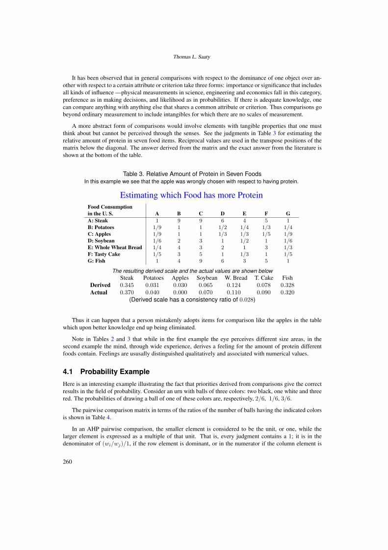
A more abstract form of comparisons would involve elements with tangible properties that one mustthink about but cannot be perceived through the senses. See the judgments in Table 3 for estimating therelative amount of protein in seven food items. Reciprocal values are used in the transpose positions of thematrix below the diagonal. The answer derived from the matrix and the exact answer from the literature isshown at the bottom of the table.
Table 3. Relative Amount of Protein in Seven FoodsIn this example we see that the apple was wrongly chosen with respect to having protein.
Estimating which Food has more ProteinFood Consumptionin the U. S. A B C D E F GA: Steak 1 9 9 6 4 5 1B: Potatoes 1/9 1 1 1/2 1/4 1/3 1/4C: Apples 1/9 1 1 1/3 1/3 1/5 1/9D: Soybean 1/6 2 3 1 1/2 1 1/6E: Whole Wheat Bread 1/4 4 3 2 1 3 1/3F: Tasty Cake 1/5 3 5 1 1/3 1 1/5G: Fish 1 4 9 6 3 5 1
The resulting derived scale and the actual values are shown belowSteak Potatoes Apples Soybean W. Bread T. Cake Fish
Derived 0.345 0.031 0.030 0.065 0.124 0.078 0.328Actual 0.370 0.040 0.000 0.070 0.110 0.090 0.320
(Derived scale has a consistency ratio of 0.028)
Thus it can happen that a person mistakenly adopts items for comparison like the apples in the tablewhich upon better knowledge end up being eliminated.
Note in Tables 2 and 3 that while in the first example the eye perceives different size areas, in thesecond example the mind, through wide experience, derives a feeling for the amount of protein differentfoods contain. Feelings are ususally distinguished qualitatively and associated with numerical values.
4.1 Probability Example
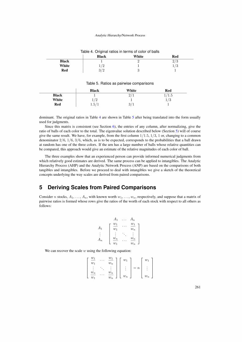
Here is an interesting example illustrating the fact that priorities derived from comparisons give the correctresults in the field of probability. Consider an urn with balls of three colors: two black, one white and threered. The probabilities of drawing a ball of one of these colors are, respectively, 2/6, 1/6, 3/6.
The pairwise comparison matrix in terms of the ratios of the number of balls having the indicated colorsis shown in Table 4.
In an AHP pairwise comparison, the smaller element is considered to be the unit, or one, while thelarger element is expressed as a multiple of that unit. That is, every judgment contains a 1; it is in thedenominator of (wi/wj)/1, if the row element is dominant, or in the numerator if the column element is
260
Analytic Hierarchy/Network Process
Table 4. Original ratios in terms of color of ballsBlack White Red
Black 1 2 2/3White 1/2 1 1/3Red 3/2 3 1
Table 5. Ratios as pairwise comparisons
Black White RedBlack 1 2/1 1/1.5White 1/2 1 1/3Red 1.5/1 3/1 1
dominant. The original ratios in Table 4 are shown in Table 5 after being translated into the form usuallyused for judgments.
Since this matrix is consistent (see Section 6), the entries of any column, after normalizing, give theratio of balls of each color to the total. The eigenvalue solution described below (Section 5) will of coursegive the same result. We have, for example, from the first column 1/1.5, 1/3, 1 or, changing to a commondenominator 2/6, 1/6, 3/6, which, as is to be expected, corresponds to the probabilities that a ball drawnat random has one of the three colors. If the urn has a large number of balls whose relative quantities canbe compared, this approach would give an estimate of the relative magnitudes of each color of ball.
The three examples show that an experienced person can provide informed numerical judgments fromwhich relatively good estimates are derived. The same process can be applied to intangibles. The AnalyticHierarchy Process (AHP) and the Analytic Network Process (ANP) are based on the comparisons of bothtangibles and intangibles. Before we proceed to deal with intangibles we give a sketch of the theoreticalconcepts underlying the way scales are derived from paired comparisons.
5 Deriving Scales from Paired Comparisons
Consider n stocks, A1, . . . , An, with known worth w1, . . . , wn, respectively, and suppose that a matrix ofpairwise ratios is formed whose rows give the ratios of the worth of each stock with respect to all others asfollows:
A1 . . . An
A1
...An
⎡⎢⎢⎢⎣
w1
w1· · · w1
wn...
. . ....
wn
w1· · · wn
wn
⎤⎥⎥⎥⎦
We can recover the scale w using the following equation:
⎡⎢⎢⎢⎣
w1
w1· · · w1
wn...
. . ....
wn
w1· · · wn
wn
⎤⎥⎥⎥⎦⎡⎢⎢⎢⎣
w1
...
wn
⎤⎥⎥⎥⎦ = n
⎡⎢⎢⎢⎣
w1
...
wn
⎤⎥⎥⎥⎦
261
Thomas L. Saaty
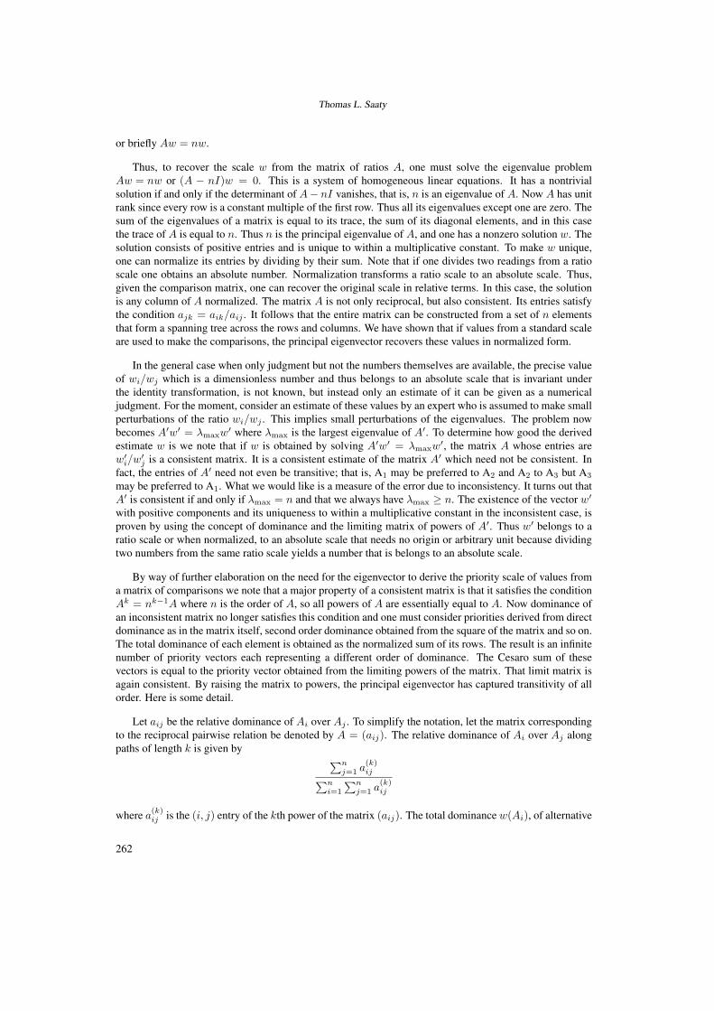
or briefly Aw = nw.
Thus, to recover the scale w from the matrix of ratios A, one must solve the eigenvalue problemAw = nw or (A − nI)w = 0. This is a system of homogeneous linear equations. It has a nontrivialsolution if and only if the determinant of A− nI vanishes, that is, n is an eigenvalue of A. Now A has unitrank since every row is a constant multiple of the first row. Thus all its eigenvalues except one are zero. Thesum of the eigenvalues of a matrix is equal to its trace, the sum of its diagonal elements, and in this casethe trace of A is equal to n. Thus n is the principal eigenvalue of A, and one has a nonzero solution w. Thesolution consists of positive entries and is unique to within a multiplicative constant. To make w unique,one can normalize its entries by dividing by their sum. Note that if one divides two readings from a ratioscale one obtains an absolute number. Normalization transforms a ratio scale to an absolute scale. Thus,given the comparison matrix, one can recover the original scale in relative terms. In this case, the solutionis any column of A normalized. The matrix A is not only reciprocal, but also consistent. Its entries satisfythe condition ajk = aik/aij . It follows that the entire matrix can be constructed from a set of n elementsthat form a spanning tree across the rows and columns. We have shown that if values from a standard scaleare used to make the comparisons, the principal eigenvector recovers these values in normalized form.
In the general case when only judgment but not the numbers themselves are available, the precise valueof wi/wj which is a dimensionless number and thus belongs to an absolute scale that is invariant underthe identity transformation, is not known, but instead only an estimate of it can be given as a numericaljudgment. For the moment, consider an estimate of these values by an expert who is assumed to make smallperturbations of the ratio wi/wj . This implies small perturbations of the eigenvalues. The problem nowbecomes A′w′ = λmaxw
′ where λmax is the largest eigenvalue of A′. To determine how good the derivedestimate w is we note that if w is obtained by solving A′w′ = λmaxw
′, the matrix A whose entries arew′i/w′j is a consistent matrix. It is a consistent estimate of the matrix A′ which need not be consistent. Infact, the entries of A′ need not even be transitive; that is, A1 may be preferred to A2 and A2 to A3 but A3
may be preferred to A1. What we would like is a measure of the error due to inconsistency. It turns out thatA′ is consistent if and only if λmax = n and that we always have λmax ≥ n. The existence of the vector w′
with positive components and its uniqueness to within a multiplicative constant in the inconsistent case, isproven by using the concept of dominance and the limiting matrix of powers of A′. Thus w′ belongs to aratio scale or when normalized, to an absolute scale that needs no origin or arbitrary unit because dividingtwo numbers from the same ratio scale yields a number that is belongs to an absolute scale.
By way of further elaboration on the need for the eigenvector to derive the priority scale of values froma matrix of comparisons we note that a major property of a consistent matrix is that it satisfies the conditionAk = nk−1A where n is the order of A, so all powers of A are essentially equal to A. Now dominance ofan inconsistent matrix no longer satisfies this condition and one must consider priorities derived from directdominance as in the matrix itself, second order dominance obtained from the square of the matrix and so on.The total dominance of each element is obtained as the normalized sum of its rows. The result is an infinitenumber of priority vectors each representing a different order of dominance. The Cesaro sum of thesevectors is equal to the priority vector obtained from the limiting powers of the matrix. That limit matrix isagain consistent. By raising the matrix to powers, the principal eigenvector has captured transitivity of allorder. Here is some detail.
Let aij be the relative dominance of Ai over Aj . To simplify the notation, let the matrix correspondingto the reciprocal pairwise relation be denoted by A = (aij). The relative dominance of Ai over Aj alongpaths of length k is given by ∑n
j=1 a(k)ij∑n
i=1
∑nj=1 a
(k)ij
where a(k)ij is the (i, j) entry of the kth power of the matrix (aij). The total dominance w(Ai), of alternative
262

Analytic Hierarchy/Network Process
i over all other alternatives along paths of all lengths is given by the infinite series
w(Ai) =∞∑
k=1
∑nj=1 a
(k)ij∑n
i=1
∑nj=1 a
(k)ij
which coincides with the Cesaro sum
limM→∞
1M
M∑k=1
∑nj=1 a
(k)ij∑n
i=1
∑nj=1 a
(k)ij
6 When is a Positive Reciprocal Matrix Consistent?In light of the foregoing, for the validity of the vector of priorities to describe response, we need greaterredundancy and therefore also a large number of comparisons. We now show that for consistency we needto make a small number of comparisons. So where is the optimum number?
We now relate the psychological idea of the consistency of judgments and its measurement, to a centralconcept in matrix theory and also to the size of our channel capacity to process information. It is theprincipal eigenvalue of a matrix of paired comparisons.
Let A = [aij ] be an n-by-n positive reciprocal matrix, so all aii = 1 and aij = 1/aji for all i, j = 1, . . . ,n. Let w = [wi] be the principal right eigenvector of A, let D = diag(w1, . . . , wn) be the n-by-n diagonalmatrix whose main diagonal entries are the entries of w, and set E ≡ D−1AD = [aijwj/wi] = [εij ].Then E is similar to A and is a positive reciprocal matrix since εij = ajiwi/wj = (aijwj/wi)−1 = 1/εij .Moreover, all the row sums of E are equal to the principal eigenvalue of A:
n∑j=1
εij =n∑
j=1
aijwj
wi=
[Aw]iwi
= λmaxwi
wi= λmax
The computation
nλmax =n∑
i=1
(n∑
i=1
εij
)=
n∑i=1
εii +∑i,j=1i �=j
(εij + εji) = n +∑i,j=1i �=j
(εij + ε−1ij ) ≥ n + 2
(n2 − n)2
= n2
reveals that λmax ≥ n. Moreover, since x + 1/x ≥ 2 for all x > 0, with equality if and only if x = 1, wesee that λmax = n if and only if all εij = 1, which is equivalent to having all aij = wi/wj .
The foregoing arguments show that a positive reciprocal matrix A has λmax ≥ n, with equality if andonly if A is consistent. As our measure of deviation of A from consistency, we choose the consistency index
μ ≡ λmax − n
n− 1
We have seen that μ ≥ 0 and μ = 0 if and only if A is consistent. We can say that as μ → 0,aij → wi/wj , or εij = aijwj/wi → 1. These two desirable properties explain the term “n” in thenumerator of μ; what about the term “n− 1” in the denominator? Since trace(A) = n is the sum of all theeigenvalues of A, if we denote the eigenvalues of A that are different from λmax by λ2, . . . , λn, we see thatn = λmax +
∑ni=2 λi, so n− λmax =
∑ni=2 λi and μ = 1
n−1
∑ni=2 λi is the average of the non-principal
eigenvalues of A.
It is an easy, but instructive, computation to show that λmax = 2 for every 2-by-2 positive reciprocalmatrix: [
1 αα−1 1
] [1 + α
(1 + α)α−1
]= 2
[1 + α
(1 + α)α−1
]
263

Thomas L. Saaty
Thus, every 2-by-2 positive reciprocal matrix is consistent.
Not every 3-by-3 positive reciprocal matrix is consistent, but in this case we are fortunate to have againexplicit formulas for the principal eigenvalue and eigenvector. For
A =
⎡⎣ 1 a b
1/a 1 c1/b 1/c 1
⎤⎦
we have λmax = 1 + d + d−1, d = (ac/b)1/3 and
w1 =bd
1 + bd + c/d, w2 =
c
d(1 + bd + c/d), w3 =
11 + bd + c/d
Note that λmax = 3 when d = 1 or c = b/a, which is true if and only if A is consistent.
In order to get some feel for what the consistency index might be telling us about a positive n-by-nreciprocal matrix A, consider the following simulation: choose the entries of A above the main diagonal atrandom from the 17 values {1/9, 1/8, . . . , 1, 2, . . . , 8, 9}. Then fill in the entries of A below the diagonalby taking reciprocals. Put ones down the main diagonal and compute the consistency index. Do this 50,000times and take the average, which we call the random index. Table 6 shows the values obtained from oneset of such simulations and also their first order differences, for matrices of size 1, 2, . . . , 15.
Table 6. Random indexOrder 1 2 3 4 5 6 7 8 9 10 11 12 13 14 15R. I. 0 0 0.52 0.89 1.11 1.25 1.35 1.40 1.45 1.49 1.52 1.54 1.56 1.58 1.59
First Order Differences 0 0.52 0.37 0.22 0.14 0.10 0.05 0.05 0.04 0.03 0.02 0.02 0.02 0.01
Figure 2 below is a plot of the first two rows of Table 6. It shows the asymptotic nature of randominconsistency.
Figure 2. Plot of Random Inconsistency
Since it would be pointless to try to discern any priority ranking from a set of random comparisonjudgments, we should probably be uncomfortable about proceeding unless the consistency index of a pair-wise comparison matrix is very much smaller than the corresponding random index value in Table 6. The
264

Analytic Hierarchy/Network Process
consistency ratio (C. R.) of a pairwise comparison matrix is the ratio of its consistency index μ to the corre-sponding random index value in Table 5. The notion of order of magnitude is essential in any mathematicalconsideration of changes in measurement. When one has a numerical value say between 1 and 10 for somemeasurement and one wants to determine whether change in this value is significant or not, one reasonsas follows: A change of a whole integer value is critical because it changes the magnitude and identityof the original number significantly. If the change or perturbation in value is of the order of a percent orless, it would be so small (by two orders of magnitude) and would be considered negligible. However ifthis perturbation is a decimal (one order of magnitude smaller) we are likely to pay attention to modifythe original value by this decimal without losing the significance and identity of the original number aswe first understood it to be. Thus in synthesizing near consistent judgment values, changes that are toolarge can cause dramatic change in our understanding, and values that are too small cause no change inour understanding. We are left with only values of one order of magnitude smaller that we can deal withincrementally to change our understanding. It follows that our allowable consistency ratio should be notmore than about 0.10. The requirement of 10% cannot be made smaller such as 1% or 0.1% without trivial-izing the impact of inconsistency. But inconsistency itself is important because without it, new knowledgethat changes preference cannot be admitted. Assuming that all knowledge should be consistent contradictsexperience that requires continued revision of understanding.
If the C. R. is larger than desired, we do three things: 1) Find the most inconsistent judgment in thematrix (for example, that judgment for which εij = aijwj/wi is largest), 2) Determine the range of valuesto which that judgment can be changed corresponding to which the inconsistency would be improved, 3)Ask the judge to consider, if he can, change his judgment to a plausible value in that range. Three methodsare plausible for this purpose. All require theoretical investigation of convergence and efficiency. The firstuses an explicit formula for the partial derivatives of the Perron eigenvalue with respect to the matrix entries.
For a given positive reciprocal matrix A = [aij ] and a given pair of distinct indices k > l, defineA(t) = [aij(t)] by akl(t) ≡ akl + t, alk(t) ≡ (alk + t)−1, and aij(t) ≡ aij for all i �= k, j �= l, soA(0) = A. Let λmax(t) denote the Perron eigenvalue of A(t) for all t in a neighborhood of t = 0 that issmall enough to ensure that all entries of the reciprocal matrix A(t) are positive there. Finally, let v = [vi]be the unique positive eigenvector of the positive matrix AT that is normalized so that vT w = 1. Then aclassical perturbation formulatells us that
dλmax(t)dt
∣∣∣∣t=0
=vT A′(0)w
vT w= vT A′(0)w = vkwl − 1
a2kl
vlwk.
We conclude that
∂λmax
∂aij= viwj − a2
jivjwi, for all i, j = 1, . . . , n.
Because we are operating within the set of positive reciprocal matrices, ∂λmax∂aji
= −∂λmax∂aij
for all i and j.Thus, to identify an entry of A whose adjustment within the class of reciprocal matrices would result in thelargest rate of change in λmax we should examine the n(n−1)/2 values {viwj−a2
jivjwi}, i > j and select(any) one of largest absolute value. If the judge is unwilling to change that judgment at all, we try with thesecond most inconsistent judgment and so on. If no judgment is changed the decision is postponed untila better understanding of the stimuli is obtained. Judges who understand the theory are always willing torevise their judgments often not the full value but partially and then examine the second most inconsistentjudgment and so on. It can happen that a judge’s knowledge does not permit one to improve his or herconsistency and more information is required to improve the consistency of judgments.
Before proceeding further, the following observations may be useful for a better understanding of theimportance of the concept of a limit on our ability to process information and also change information.
265

Thomas L. Saaty
The quality of response to stimuli is determined by three factors. Accuracy or validity, consistency, andefficiency or amount of information generated. Our judgment is much more sensitive and responsive tolarge perturbations. When we speak of perturbation, we have in mind numerical change from consistentratios obtained from priorities. The larger the inconsistency and hence also the larger the perturbations inpriorities, the greater our sensitivity to make changes in the numerical values assigned. Conversely, thesmaller the inconsistency, the more difficult it is for us to know where the best changes should be madeto produce not only better consistency but also better validity of the outcome. Once near consistency isattained, it becomes uncertain which coefficients should be perturbed by small amounts to transform a nearconsistent matrix to a consistent one. If such perturbations were forced, they could be arbitrary and thusdistort the validity of the derived priority vector in representing the underlying decision.
The third row of Table 6 gives the differences between successive numbers in the second row. Figure 3is a plot of these differences and shows the importance of the number seven as a cutoff point beyondwhich the differences are less than 0.10 where we are not sufficiently sensitive to make accurate changesin judgment on several elements simultaneously. Thus in general, one should only compare a few elements(about seven), and when their number is larger, one should put them into groups with a common elementfrom one group to the next so that its weight can be used as a pivot to combine the final weights.
Figure 3. Plot of First Differences in Random Inconsistency
7 Second Affirmation through the Eigenvector
Stability of the principal eigenvector also imposes a limit on channel capacity and also highlights the im-portance of homogeneity. To a first order approximation, perturbation Δw1 in the principal eigenvector w1
due to a perturbation ΔA in the matrix A where A is inconsistent is given by Wilkinson [20]:
Δw1 =n∑
j=2
(vTj ΔAw1/(λ1 − λj)vT
j wj)wj
Here T indicates transposition. The eigenvector w1 is insensitive to perturbation in A, if 1) the numberof terms n is small, 2) if the principal eigenvalue λ1 is separated from the other eigenvalues λj , hereassumed to be distinct (otherwise a slightly more complicated argument given below can be made) and, 3)if none of the products vT
j wj of left and right eigenvectors is small but if one of them is small, they are all
266

Analytic Hierarchy/Network Process
small. However, vT1 w1, the product of the normalized left and right principal eigenvectors of a consistent
matrix is equal to n that as an integer is never very small. If n is relatively small and the elements beingcompared are homogeneous, none of the components of w1 is arbitrarily small and correspondingly, none ofthe components of vT
1 is arbitrarily small. Their product cannot be arbitrarily small, and thus w is insensitiveto small perturbations of the consistent matrix A. The conclusion is that n must be small, and one mustcompare homogeneous elements.
When the eigenvalues have greater multiplicity than one, the corresponding left and right eigenvectorswill not be unique. In that case the cosine of the angle between them which is given by vT
i wi corresponds toa particular choice of wi and vi . Even when wi and vi correspond to a simple λi they are arbitrary to withina multiplicative complex constant of unit modulus, but in that case |vT
i wi| is fully determined. Becauseboth vectors are normalized, we always have |vT
i wi| < 1.
8 Axioms
For completeness we have borrowed the axioms section from Chapter 10 of my book Fundamentals of
Decision Making [12]. The reader might consult that book for a full description and results derived fromthe axioms, but the editors thought it would be useful to include them here for ready reference.
Let A be a finite set of n elements called alternatives. Let C be a set of properties or attributes withrespect to which elements in A are compared. A property is a feature that an object or individual possesseseven if we are ignorant of this fact, whereas an attribute is a feature we assign to some object: it is aconcept. Here we assume that properties and attributes are interchangeable, and we generally refer to themas criteria. A criterion is a primitive concept.
When two objects or elements in A are compared according to a criterion C in C, we say that we areperforming binary comparisons. Let >C be a binary relation on A representing “more preferred than” or“dominates” with respect to a criterion C in C. Let ∼C be the binary relation “indifferent to” with respectto a criterion C in C. Hence, given two elements, Ai, Aj ∈ A, either Ai >C Aj or Aj >C Ai or Ai ∼C Aj
for all C ∈ C. We use Ai >∼C Aj to indicate more preferred or indifferent. A given family of binary
relations >C with respect to a criterion C in C is a primitive concept. We shall use this relation to derivethe notion of priority or importance both with respect to one criterion and also with respect to several.
LetP be the set of mappings from A×A to R+ (the set of positive reals). Let f : C→ P. Let PC ∈ f(C)
for C ∈ C. PC assigns a positive real number to every pair (Ai, Aj) ∈ A× A. Let PC(Ai, Aj)/aij ∈ R+,
Ai, Aj ∈ A. For each C ∈ C, the triple (A×A, R+, PC) is a fundamental or primitive scale. A fundamentalscale is a mapping of objects to a numerical system.
Definition 1. For all Ai, Aj ∈ A and C ∈ CAi >C Aj if and only if PC(Ai, Aj) > 1,
Ai ∼C Aj if and only if PC(Ai, Aj) = 1.
If Ai >C Aj , we say that Ai dominates Aj with respect to C ∈ C. Thus PC represents the intensity orstrength of preference for one alternative over another.
8.1 Reciprocal Axiom
Axiom 1. For all Ai, Aj ∈ A and C ∈ C
PC(Ai, Aj) =1
PC(Aj , Ai)
267

Thomas L. Saaty
Whenever we make paired comparisons, we need to consider both members of the pair to judge therelative value. The smaller or lesser one is first identified and used as the unit for the criterion in question.The other is then estimated as a not necessarily integer multiple of that unit. Thus, for example, if one stoneis judged to be five times heavier than another, then the other is automatically one fifth as heavy as the firstbecause it participated in making the first judgment. The comparison matrices that we consider are formedby making paired reciprocal comparisons. It is this simple yet powerful means of resolving multicriteriaproblems that is the basis of the AHP.
Let A = (aij)/(PC(Ai, Aj)) be the set of paired comparisons of the alternatives with respect to acriterion C ∈ C. By Axiom 1, A is a positive reciprocal matrix. The object is to obtain a scale of relative
dominance (or rank order) of the alternatives from the paired comparisons given in A.
There is a natural way to derive the relative dominance of a set of alternatives from a pairwise compari-son matrix A.
Definition 2. Let RM(n) be the set of (n×n) positive reciprocal matrices A = (aij)/(PC(Ai, Aj)) for all
C ∈ C. Let [0, 1]n be the n-fold cartesian product of [0, 1] and let Ψ(A) : RM(n) → [0, 1]n for A ∈ RM(n),
Ψ(A) is an n-dimensional vector whose components lie in the interval [0, 1]. The triple (RM(n), [0, 1]n, Ψ)is a derived scale. A derived scale is a mapping between two numerical relational systems.
It is important to point out that the rank order implied by the derived scale Ψ may not coincide with theorder represented by the pairwise comparisons. Let Ψi(A) be the ith component of Ψ(A). It denotes therelative dominance of the ith alternative. By definition, for Ai, Aj ∈ A, Ai >C Aj implies PC(Ai, Aj) > 1.However, if PC(Ai, Aj) > 1, the derived scale could imply that Ψj(A) > Ψi(A). This occurs if rowdominance does not hold, i.e., for Ai, Aj ∈ A, and C ∈ C, PC(Ai, Aj) ≥ PC(Aj , Ak) does not hold forall Ak ∈ A. In other words, it may happen that PC(Ai, Aj) > 1, and for some Ak ∈ A we have
PC(Ai, Ak) < PC(Aj , Ak)
A more restrictive condition is the following:
Definition 3. The mapping PC is said to be consistent if and only if PC(Ai, Aj)PC(Aj , Ak)=PC(Ai, Ak)for all i, j, and k. Similarly the matrix A is consistent if and only if aijajk = aik for all i, j, and k.
If PC is consistent, then Axiom 1 automatically follows and the rank order induced by Ψ coincides withpairwise comparisons.
Luis Vargas has proposed, through personal communication with the author, that the following “behav-ioral” independence axiom could be used instead of the more mathematical reciprocal axiom that wouldthen follow as a theorem. However, the reciprocal relation does not imply independence as defined by him,and unless one wishes to assume independence, one should retain the reciprocal axiom.
Two alternatives Ai and Aj are said to be mutually independent with respect to a criterion C ∈ C if andonly if, for any Ak the paired comparison of the component {Ai, Aj} with respect to Ak satisfies
PC [{Ai, Aj}, Ak] = PC(Ai, Ak)PC(Aj , Ak)
andPC [Ak, {Ai, Aj}] = PC(Ak, Ai)PC(Ak, Aj)
A set of alternatives is said to be independent if they are mutually independent.
Axiom 1. All the alternatives in A are independent.
268

Analytic Hierarchy/Network Process
8.2 Hierarchic Axioms
Definition 4. A partially ordered set is a set S with a binary relation ≤ which satisfies the following
conditions:
a. Reflexive: For all x ∈ S, x ≤ x,
b. Transitive: For all x, y, z ∈ S, if x ≤ y and y ≤ z then x ≤ z,
c. Antisymmetric: For all x, y ∈ S, if x ≤ y and y ≤ x then x = y (x and y coincide).
Definition 5. For any relation x ≤ y (read, y includes x) we define x < y to mean that x ≤ y and x �= y.
y is said to cover (dominate) x if x < y and if x < t < y is possible for no t.
Partially ordered sets with a finite number of elements can be conveniently represented by a directedgraph. Each element of the set is represented by a vertex so that an arc is directed from y to x if x < y.
Definition 6. A subset E of a partially ordered set S is said to be bounded from above (below) if there is
an element s ∈ S such that x ≤ s (≥ s) for every x ∈ E. The element s is called an upper (lower) bound of
E. We say that E has a supremum (infimum) if it has upper (lower) bounds and if the set of upper (lower)
bounds U (L) has an element u1 (l1) such that u1 ≤ u for all u ∈ U (l1 ≥ l for all l ∈ L).
Definition 7. Let H be a finite partially ordered set with largest element b. The set H is a hierarchy if it
satisfies the following conditions:
1. There is a partition of H into sets called levels {Lk, k = 1, 2, . . . , h}, where L1 = {b}.2. x ∈ Lk implies x− ⊆ Lk+1, where x− = {y | x covers y}, k = 1, 2, . . . , h− 1.
3. x ∈ Lk implies x+ ⊆ Lk−1, where x+ = {y | y covers x}, k = 2, 3, . . . , h.
Definition 8. Given a positive real number ρ ≥ 1, a nonempty set x− ⊆ Lk+1 is said to be ρ-homogeneous
with respect to x ∈ Lk if for every pair of elements y1, y2 ∈ x−, 1/ρ ≤ PC(y1, y2) ≤ ρ. In particular the
reciprocal axiom implies that PC(yi, yi) = 1.
Axiom 2. Given a hierarchy H, x ∈ H and x ∈ Lk, x− ⊆ Lk+1 is ρ-homogeneous for k = 1, . . . , h− 1.
Homogeneity is essential for comparing similar things, as the mind tends to make large errors in compar-ing widely disparate elements. For example, we cannot compare a grain of sand with an orange accordingto size. When the disparity is great, the elements are placed in separate components of comparable size,giving rise to the idea of levels and their decomposition. This axiom is closely related to the well-knownArchimedean property which says that forming two real numbers x and y with x < y, there is an integer nsuch that nx ≥ y, or n ≥ y/x.
The notions of fundamental and derived scales can be extended to x ∈ Lk, x− ⊆ Lk+1 replacing C andA, respectively. The derived scale resulting from comparing the elements in x− with respect to x is calleda local derived scale or local priorities. Here no irrelevant alternative is included in the comparisons, andsuch alternatives are assumed to receive the value of zero in the derived scale.
Given Lk, Lk+1 ⊆ H, let us denote the local derived scale for y ∈ x− and x ∈ Lk by Ψk+1(y|x),k = 2, 3, . . . , h− 1. Without loss of generality we may assume that
∑y0x− Ψk+1(y|x) = 1. Consider the
matrix Ψk(Lk|Lk−1) whose columns are local derived scales of elements in Lk with respect to elements inLk−1.
Definition 9. A set A is said to be outer dependent on a set C if a fundamental scale can be defined on Awith respect to every c ∈ C.
269

Thomas L. Saaty
Decomposition implies containment of the small elements by the large components or levels. In turn,this means that the smaller elements depend on the outer parent elements to which they belong, whichthemselves fall in a large component of the hierarchy. The process of relating elements (e.g., alternatives)in one level of the hierarchy according to the elements of the next higher level (e.g., criteria) expressesthe outer dependence of the lower elements on the higher elements. This way comparisons can be madebetween them. The steps are repeated upward in the hierarchy through each pair of adjacent levels to thetop element, the focus or goal.
The elements in a level may depend on one another with respect to a property in another level. Input-output dependence of industries (e.g., manufacturing) demonstrates the idea of inner dependence. This maybe formalized as follows:
Definition 10. Let A be outer dependent on C. The elements in A are said to be inner dependent with
respect to C ∈ C if for some A ∈ A, A is outer dependent on A.
Axiom 3. Let H be a hierarchy with levels L1, L2, . . . , Lh. For each Lk, k = 1, 2, . . . , h− 1,
1. Lk+1 is outer dependent on Lk
2. Lk is not outer dependent on Lk+1
3. Lk+1 is not inner dependent with respect to any x ∈ Lk.
8.3 Principle of Hierarchic CompositionIf Axiom 3 holds, the global derived scale (rank order) of any element in H is obtained from its componentin the corresponding vector of the following:
Ψ1(b) = 1
Ψ2(L2) = Ψ2(b−|b)...
...Ψk(Lk) = Ψk(Lk|Lk−1), Ψk−1(Lk−1), k = 3, . . . , h
Were one to omit Axiom 3, the Principle of Hierarchic Composition would no longer apply because ofouter and inner dependence among levels or components which need not form a hierarchy. The appropriatecomposition principle is derived from the supermatrix approach explained below, of which the Principle ofHierarchic Composition is a special case.
A hierarchy is a special case of a system, defined as follows:
Definition 11. Let H be a family of nonempty sets C1, C2, . . . , Cn where Ci consists of the elements
{eij , j = 1, . . . , mi}, i = 1, 2, . . . , n. H is a system if it is a directed graph whose vertices are Ci
and whose arcs are defined through the concept of outer dependence; thus, given two components Ci and
Cj ∈ H, there is an arc from Ci to Cj if Cj is outer dependent on Ci.
Axiom 3’. Let H be a system consisting of the subsets C1, C2, . . . , Cn. For each Ci there is some Cj so
that either Ci is outer dependent on Cj or Cj is outer dependent on Ci, or both.
Note that Ci may be outer dependent on Ci, which is equivalent to inner dependence in a hierarchy.Actually Axiom 3’ would by itself be adequate without Axiom 3. We have separated them because of theimportance of hierarchic structures, which are more widespread at the time of this writing than are systemswith feedback.
Many of the concepts derived for hierarchies also relate to systems with feedback. Here one needs tocharacterize dependence among the elements. We now give a criterion for this purpose.
270

Analytic Hierarchy/Network Process
Let DA ⊆ A be the set of elements of A outer dependent on A ∈ A. Let ΨAi,C(Aj), Aj ∈ A be thederived scale of the elements of A with respect to Ai ∈ A, for a criterion C ∈ C. Let ΨC(Aj), Aj ∈ A bethe derived scale of the elements of A with respect to a criterion C ∈ C. We define the dependence weight
ΦC(Aj) =∑
Ai∈DAj
ΨAiC(Aj)ΨC(Ai)
If the elements of A are inner dependent with respect to C ∈ C, then ΨC(Ai) �= ΨC(Aj) for some Aj ∈ A.
Hierarchic composition yields multilinear forms which are of course nonlinear and have the form∑ii,...,ip
xi11 xi2
2 · · ·xipp
The richer the structure of a hierarchy in breadth and depth the more complex are the derived multilinearforms from it. There seems to be a good opportunity to investigate the relationship obtained by compositionto covariant tensors and their algebraic properties. More concretely we have the following covariant tensorfor the priority of the ith element in the hth level of the hierarchy.
whi =
Nh−1,...,N1∑i2,...,ih−1=1
wh−1i1,i2
· · ·w2ih−2ih−1
w1ih−1
ii ≡ i
The composite vector for the entire hth level is represented by the vector with covariant tensorial compo-nents. Similarly, the left eigenvector approach to a hierarchy gives rise to a vector with contravariant tensorcomponents. Tensors, are generalizations of scalars (which have no indices), vectors (which have a singleindex), and matrices or arrays (which have two indices) to an arbitrary number of indices. They are widelyknown and used in physics and engineering.
8.4 ExpectationsExpectations are beliefs about the rank of alternatives derived from prior knowledge. Assume that a decisionmaker has a ranking, arrived at intuitively, of a finite set of alternatives A with respect to prior knowledgeof criteria C.
Axiom 4.
1. Completeness: C ⊂ H− Lh, A = Lh.
2. Rank: To preserve rank independently of what and how many other alternatives there may be. Alter-
natively, to allow rank to be influenced by the number and the measurements of alternatives that are
added to or deleted from the set.
This axiom simply says that those thoughtful individuals who have reasons for their beliefs shouldmake sure that their ideas are adequately represented for the outcome to match these expectations; i.e.,all criteria are represented in the hierarchy. It assumes neither that the process is rational nor that it canaccommodate only a rational outlook. People could have expectations that are branded irrational in someoneelse’s framework. It also says that the rank of alternatives depends both on the expectations of the decisionmaker and on the nature of a decision problem.
Now we illustrate how the foregoing theory can be used in practice. The following example uses hier-archies to model the Iran crisis in the context of the Middle East conflict and the fear of Israel and the Westabout Iran having nuclear weapons by refining fissionable material in quantities beyond what is required forsatisfying Iran’s energy needs.
271

Thomas L. Saaty
9 Example: AHP Analysis of Strategies towards Iran
The threat of war in Iran is a complex and controversial issue, involving many actors in different regionsand several possible courses of action. Nearly 40 people were involved in the exercise done in October2007. They were divided into groups of 4 or 5 and each of these groups worked out the model and derivedresults for a designated merit: benefits, opportunities, costs or risks. In the end there were two outcomes foreach merit which were combined using the geometric mean as described in the section on group decisionmaking and then the four resulting outcomes were combined into a single overall outcome as describedbelow. It should be understood that this is only an exercise to illustrate use of the method and no real lifeconclusions should be drawn from it primarily because it did not involve political expert and negotiatorsfrom all the interested parties. Its conclusions should be taken as hypotheses to be further tested. In thesummer of 2008 many people, including authors who write from Israel who want to prevent Iran fromacquiring nuclear power the most, consider that attacking Iran would lead to great harm to the economiesof the world because nearly 45% of the world’s oil flows out of the Persian Gulf, and Iran would then makesure of its disruption.
9.1 Creating the Model
A model for determining the policy to pursue towards Iran seeking to obtain weapon grade nuclear materialwas designed using a benefits (B), opportunities (O), costs (C), and risks (R) or combined (BOCR) model.The benefits model shows which alternative would be most beneficial, the opportunities model shows whichalternative has the greatest potential for benefits, the costs model (costs may include monetary, human andintangible costs) shows which alternative would be most costly and the risks model shows which alternativehas the highest potential costs.
9.2 Strategic Criteria
Strategic Criteria are used to evaluate the BOCR merits of all decisions by a decision maker. They are theoverriding criteria that individuals, corporations or governments use to determine which decision to makefirst, and what are the relative advantages and disadvantages of that decision.
For policy towards Iran, the BOCR model structured by the group is evaluated using the strategic criteriaof World Peace (0.361), Regional Stability (0.356), Reduce Volatility (0.087) and Reduce Escalation of
Middle East Problem (0.196). The priorities of the strategic criteria indicated in parentheses next to each,are obtained from a pairwise comparisons matrix with respect to the goal of long term peace in the world.
9.3 Control Criteria
The BOCR model is evaluated using the control criteria (focusing thought to answer the question in makingpairwise comparisons): Economic, Political, Rule of Law and Security. They are the criteria for which weare able to represent the different kinds of influences that we are able to perceive which later need to becombined into an overall influence using AHP/ANP calculations.
9.4 Actors
The countries mainly concerned with this problem are: the US, Iran, Russia & China, Middle East countriesand Israel.
9.5 Alternatives
The group identified six Alternatives:
272

Analytic Hierarchy/Network Process
(1) It is reasonable to undertake Aerial Strikes towards Iran
(2) Economic Sanctions should be applied against Iran
(3) The Actors should carry out Ground Invasion of Iran
(4) Israeli Action towards Iran
(5) To do Nothing, leaving everything so as it is
(6) To make efforts to make a Regime Change
9.6 BOCR ModelsWith a view to saving space we do not give all the hierarchies and their matrices of judgments. In thisexercise it was determined to keep the structure simple by using the same structure for all four merits (seeFigure 4) albeit with different judgments. In particular for the costs and risks one asks the question whichis more (not less) costly or risky, and in the end subtract the corresponding values from those of benefitsand opportunities. The analysis derives four rankings of the alternatives, one for each of the BOCR merits.Following that one must obtain priorities for the BOCRs themselves in terms of the strategic criteria anduse the top ranked alternative for each merit in order to think about that merit and then use those prioritiesto weigh and synthesize the alternatives. The priorities of the alternatives are proportional to the priority ofthe top ranked alternative, thus they would all be multiplied by the same number that is the priority of themerit.
Figure 4. Costs Hierarchy to Choose the Best Strategy towards Iran
It is important to note again that usually for a general decision problem each merit would have a differentstructure than the other merits. However, for the sake of expediency in this decision, the group decided touse the same structure with the appropriate formulation of the questions to provide the judgments.
9.7 Judgments and ComparisonsAs previously mentioned, a judgment is an expression of opinion about the dominance (importance, pref-erence or likelihood) of one element over another. It is done every day through verbal expression that hassome quantitative significance that we need to use to combine the many dominance judgments involved ina decision. The set of all such judgments in making comparisons with respect to a single property or goalcan be represented by means of a square matrix in which the set of elements is compared. It is a way oforganizing all the judgments with respect to some property to be processed and synthesized along with othermatrices of comparisons involved in the decision. Each judgment represents the dominance of an element
273

Thomas L. Saaty
in the left column of the matrix over an element in the row on top. It reflects the answers to two questions:which of the two elements is more important with respect to a higher level criterion, and how strongly.
As usual with the AHP, in the models of benefits, opportunities, cost, and risks the group comparedthe criteria and subcriteria according to their relative importance with respect to the parent element in theadjacent upper level. For example, the entries in the matrix shown in Table 7 are responses to the question:which control criterion is more important with respect to choosing the best strategy towards Iran and howstrongly? Here economic costs are moderately more important than political costs and are assigned theabsolute number 3 in the (1, 2) or first-row second-column position. Three signifies three times more.The reciprocal value is automatically entered in the (2, 1) position, where political costs on the left arecompared with economic costs at the top. Similarly a 5, corresponding to strong dominance or importance,is assigned to security costs over political costs in the (4, 2) position, and a 2, corresponding to weak orslight dominance, is assigned to the costs of rule of law over political costs in the (3, 2) position withcorresponding reciprocals in the transpose positions of the matrix.
Judgments in a matrix may not be consistent. In eliciting judgments, one makes redundant comparisonsto improve the validity of the answer, given that respondents may be uncertain or may make poor judgmentsin comparing some of the elements. Redundancy gives rise to multiple comparisons of an element with otherelements and hence to numerical inconsistencies. The group first made all the comparisons using semanticterms from the fundamental scale and then translated them to the corresponding numbers.
Table 7. Judgment Matrix for the Control Criteria of the Costs Hierarchy
Choosing best strategytowards Iran (costs) Economic Political Rule of Law Security Normalized
PrioritiesEconomic 1 3 1/2 1/3 0.173Political 1/3 1 1/2 1/5 0.087Rule of Law 2 2 1 1/3 0.222Security 3 5 3 1 0.518
C. R. = 0.049
For example, where we compare security costs with economic costs and with political costs, we havethe respective judgments 3 and 5. Now if x = 3y and x = 5z then 3y = 5z or y = 5/3z. If the judgeswere consistent, economic costs would be assigned the value 5/3 instead of the 3 given in the matrix. Thusthe judgments are inconsistent. In fact, we are not sure which judgments are the accurate ones and whichare the cause of the inconsistency. However, these can be determined in a systematic way and improved byinterrogating the decision maker.
The process is repeated for all the matrices by asking the appropriate dominance or importance question.For example, the entries in the judgment matrix shown in Table 8 are responses to the question: which partyis more committed to ensure security?
Here US security costs are regarded as extremely more important than the security costs for Iran, and 9is entered in the (5, 1) position and 1/9 in the (1, 5) position.
In comparing the six strategies (alternatives) towards Iran, we asked members of the decision groupwhich strategy in their opinion would be more costly for each of the actors. For example, for the USA,we obtained a matrix of paired comparisons in Table 9 in which Ground Invasion is the most expensivestrategy. On the contrary, regime change and doing nothing are the least costly ones. In this examplethe criteria (here the different countries) are assumed to be independent of the alternatives and hence thepriorities of alternatives are given in ideal form by dividing by the largest priority among them. Here groundinvasion would be the most costly.
274
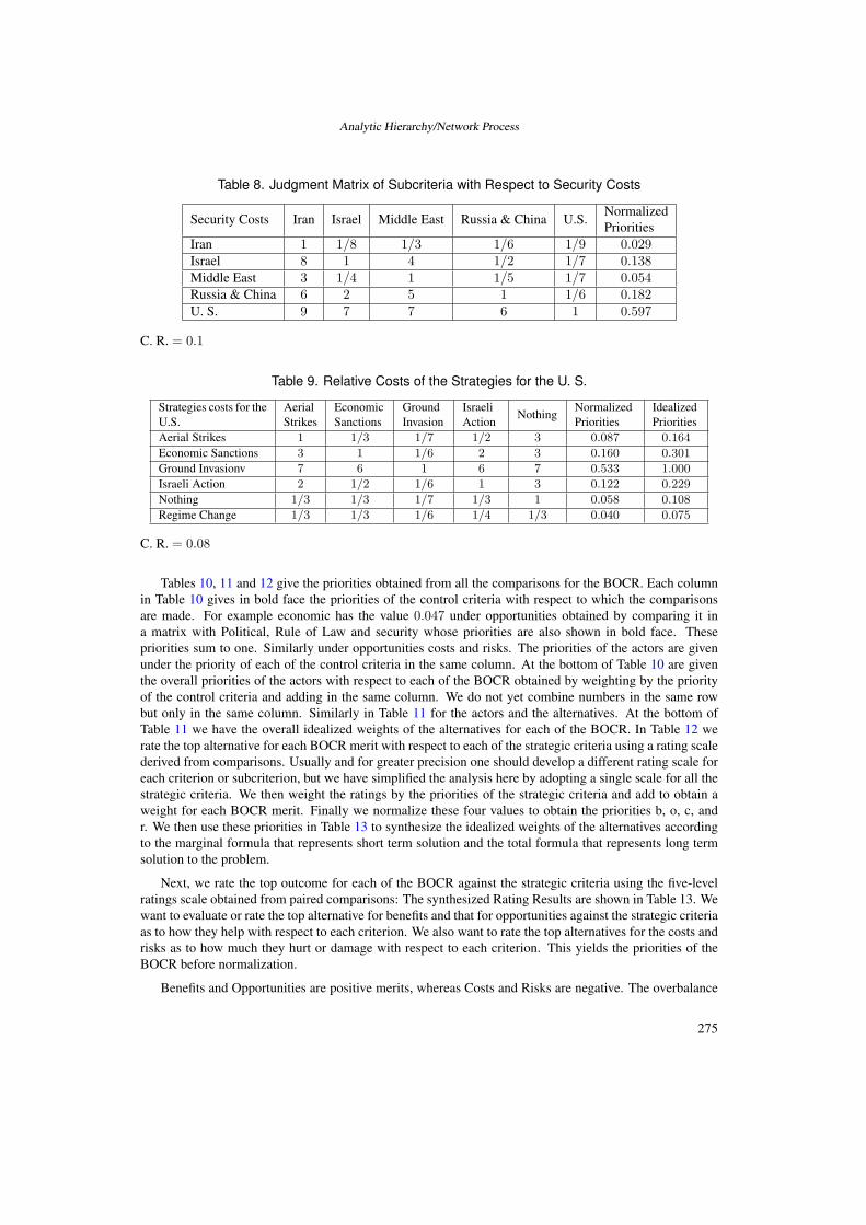
Analytic Hierarchy/Network Process
Table 8. Judgment Matrix of Subcriteria with Respect to Security Costs
Security Costs Iran Israel Middle East Russia & China U.S.NormalizedPriorities
Iran 1 1/8 1/3 1/6 1/9 0.029Israel 8 1 4 1/2 1/7 0.138Middle East 3 1/4 1 1/5 1/7 0.054Russia & China 6 2 5 1 1/6 0.182U. S. 9 7 7 6 1 0.597
C. R. = 0.1
Table 9. Relative Costs of the Strategies for the U. S.
Strategies costs for theU.S.
AerialStrikes
EconomicSanctions
GroundInvasion
IsraeliAction
NothingNormalizedPriorities
IdealizedPriorities
Aerial Strikes 1 1/3 1/7 1/2 3 0.087 0.164
Economic Sanctions 3 1 1/6 2 3 0.160 0.301
Ground Invasionv 7 6 1 6 7 0.533 1.000
Israeli Action 2 1/2 1/6 1 3 0.122 0.229
Nothing 1/3 1/3 1/7 1/3 1 0.058 0.108
Regime Change 1/3 1/3 1/6 1/4 1/3 0.040 0.075
C. R. = 0.08
Tables 10, 11 and 12 give the priorities obtained from all the comparisons for the BOCR. Each columnin Table 10 gives in bold face the priorities of the control criteria with respect to which the comparisonsare made. For example economic has the value 0.047 under opportunities obtained by comparing it ina matrix with Political, Rule of Law and security whose priorities are also shown in bold face. Thesepriorities sum to one. Similarly under opportunities costs and risks. The priorities of the actors are givenunder the priority of each of the control criteria in the same column. At the bottom of Table 10 are giventhe overall priorities of the actors with respect to each of the BOCR obtained by weighting by the priorityof the control criteria and adding in the same column. We do not yet combine numbers in the same rowbut only in the same column. Similarly in Table 11 for the actors and the alternatives. At the bottom ofTable 11 we have the overall idealized weights of the alternatives for each of the BOCR. In Table 12 werate the top alternative for each BOCR merit with respect to each of the strategic criteria using a rating scalederived from comparisons. Usually and for greater precision one should develop a different rating scale foreach criterion or subcriterion, but we have simplified the analysis here by adopting a single scale for all thestrategic criteria. We then weight the ratings by the priorities of the strategic criteria and add to obtain aweight for each BOCR merit. Finally we normalize these four values to obtain the priorities b, o, c, andr. We then use these priorities in Table 13 to synthesize the idealized weights of the alternatives accordingto the marginal formula that represents short term solution and the total formula that represents long termsolution to the problem.
Next, we rate the top outcome for each of the BOCR against the strategic criteria using the five-levelratings scale obtained from paired comparisons: The synthesized Rating Results are shown in Table 13. Wewant to evaluate or rate the top alternative for benefits and that for opportunities against the strategic criteriaas to how they help with respect to each criterion. We also want to rate the top alternatives for the costs andrisks as to how much they hurt or damage with respect to each criterion. This yields the priorities of theBOCR before normalization.
Benefits and Opportunities are positive merits, whereas Costs and Risks are negative. The overbalance
275

Thomas L. Saaty
Table 10. Priorities of the Actors with respect to Control Criteria of BOCR groups
Control Criteria Actors BENEFITS OPPORTUNITIES COSTS RISKSEconomic 0.047 0.626 0.174 0.209
Iran 0.031 0.066 0.129 0.321Israel 0.259 0.041 0.036 0.126
Middle East 0.166 0.233 0.087 0.306Russia & China 0.095 0.120 0.425 0.075
US 0.449 0.540 0.324 0.173Political 0.128 0.156 0.087 0.033
Iran 0.043 0.201 0.082 0.506Israel 0.311 0.125 0.226 0.1454
Middle East 0.133 0.494 0.067 0.248Russia & China 0.079 0.090 0.152 0.045
US 0.433 0.090 0.483 0.056Rule of Law 0.246 0.043 0.222 0.066
Iran 0.031 0.114 0.044 0.317Israel 0.347 0.415 0.218 0.118
Middle East 0.132 0.169 0.060 0.443Russia & China 0.101 0.051 0.119 0.059
US 0.389 0.251 0.559 0.063Security 0.579 0.175 0.518 0.692
Iran 0.068 0.131 0.029 0.200Israel 0.115 0.298 0.138 0.200
Middle East 0.165 0.308 0.054 0.200Russia & China 0.407 0.106 0.181 0.200
US 0.245 0.156 0.597 0.200OVERALL
Iran 0.031 0.100 0.054 0.243Israel 0.259 0.115 0.204 0.177
Middle East 0.166 0.284 0.153 0.240Russia & China 0.095 0.110 0.275 0.159
US 0.449 0.390 0.314 0.180
of weights is negative for Ground Invasion and Israeli Action and is positive for Aerial Strikes, EconomicSanctions, doing Nothing and Regime Change. As a result, in the current situation doing Nothing turns outto be the best alternative and Ground Invasion is the worst.
9.8 Sensitivity Analysis
There are many ways of doing sensitivity analysis, we show one of them here. Sensitivity graphs for BOCRgroups are shown in Figures 5, (a,b,c,d) respectively. From the software program Superdecisions we seethat the results obtained by perturbing the priorities of each of the benefits and opportunities, costs andrisks are stable. The model is sensitive to changes of priorities in the BOCR merits. As the priority ofCosts increases, the alternative ‘Israeli Action’ becomes more preferred than ‘Ground Invasion’ and ‘AerialStrikes’ becomes more important than ‘Economic Sanctions’. On the other hand, as the priority of Risksincreases, the last two alternatives ‘Israeli Action’ and ‘Ground Invasion’ trade places in the overall orderof ranking. Results obtained for Benefits and Opportunities are stable and ‘Nothing’ remains the bestalternative.
276

Analytic Hierarchy/Network Process
Table 11. Priorities of the Alternatives with respect to the Actors in BOCR groups
Actors Alternatives BENEFITS OPPORTUNITIES COSTS RISKSIran 0.031 0.100 0.054 0.243
Aerial Strikes 1.000 0.078 0.115 0.701Economic Sanctions 1.000 0.452 0.260 1.000Ground Invasion 1.000 0.057 1.000 0.294Israeli Action 1.000 0.142 0.149 0.762Nothing 1.000 1.000 0.068 0.239Regime Change 1.000 0.220 0.362 0.882
Israel 0.259 0.115 0.204 0.177Aerial Strikes 0.214 0.359 0.212 0.240Economic Sanctions 0.463 0.069 0.120 0.209Ground Invasion 0.128 0.228 0.355 0.385Israeli Action 0.070 0.104 1.000 1.000Nothing 0.177 0.062 0.210 0.153Regime Change 1.000 1.000 0.130 0.052
Middle East 0.166 0.284 0.153 0.240Aerial Strikes 0.095 0.168 0.257 0.186Economic Sanctions 0.357 0.676 0.132 0.073Ground Invasion 0.159 0.196 1.000 0.328Israeli Action 0.131 0.062 0.483 1.000Nothing 1.000 0.371 0.111 0.068Regime Change 0.702 1.000 0.175 0.045
Russia & China 0.095 0.110 0.275 0.159Aerial Strikes 0.778 0.141 0.114 0.190Economic Sanctions 0.825 0.259 0.215 0.057Ground Invasion 0.331 0.174 1.000 0.379Israeli Action 1.000 0.122 0.160 1.000Nothing 0.559 1.000 0.071 0.072Regime Change 0.303 0.154 0.411 0.086
US 0.449 0.390 0.314 0.180Aerial Strikes 0.167 1.000 0.164 0.133Economic Sanctions 0.231 0.094 0.301 0.076Ground Invasion 0.130 0.285 1.000 0.388Israeli Action 0.165 0.050 0.229 1.000Nothing 1.000 0.150 0.108 0.079Regime Change 0.130 0.417 0.075 0.038
OVERALLAerial Strikes 0.402 0.891 0.179 0.259Economic Sanctions 0.586 0.496 0.271 0.221Ground Invasion 0.258 0.378 1.000 0.368Israeli Action 0.414 0.136 0.365 1.000Nothing 1.000 0.666 0.124 0.112Regime Change 0.651 1.000 0.189 0.165
It has been recently reported in the media that the world economy would suffer greatly were Iran to beattacked militarily. This appears to be in line with current US military thinking who may or may not have
277

Thomas L. Saaty
Table 12. Ratings with Respect to Strategic Criteria of Top Alternatives for BOCR meritsVery High (1), High (0.619), Medium (0.381), Low (0.238), Very Low (0.143)
Worldpeace
(0.362)
RegionalStability(0.356)
ReduceVolatility(0.087)
Reduce Escalationof the Middle EastConflict (0.196)
Priorities NormalizedPriorities
Benefits Very High High High Medium 0.710 0.254
Opportunities Medium Low Medium Medium 0.330 0.118
Costs Very High Very High Very High Medium 0.878 0.314
Risks Very High Very High Very High Medium 0.878 0.314
Table 13. Synthesis of the Alternatives’ Overall Priorities for the Four BOCR Merits
BENEFITS OPPORTUNITIES COSTS RISKS BO/CRbB + oO−cC− rR
b = 0.254 o = 0.118 c = 0.314 r = 0.314
Aerial Strikes 0.402 0.891 0.179 0.259 7.711 0.069
Economic Sanc-tions
0.586 0.496 0.271 0.221 4.841 0.053
Ground Invasion 0.258 0.378 1.000 0.368 0.265 −0.319
Israeli Action 0.414 0.136 0.365 1.000 0.155 −0.308
Nothing 1.000 0.666 0.124 0.112 48.077 0.258
Regime Change 0.651 1.000 0.189 0.165 20.814 0.172
used this process, of which they are well aware, to arrive at their conclusion.
10 Networks, Dependence and Feedback
In Figure 6, we exhibit a hierarchy and a network [11, 13]. A hierarchy is comprised of a goal, levels ofelements and connections between the elements. These connections are oriented only to elements in lowerlevels. A network has clusters of elements, with the elements in one cluster being connected to elements inanother cluster (outer dependence) or the same cluster (inner dependence). A hierarchy is a special case ofa network with connections going only in one direction.
There are two kinds of influence: outer and inner. In the first, one compares the influence of elementsin a cluster on elements in another cluster with respect to a control criterion. It is assumed that influencesare decomposed into recognizable basic influences known as control criteria such as economic, political,technological, environmental and so on in terms of which all the comparisons and ranking of the alternativesare made. In inner influence one compares the influence of elements in a group on each one. For exampleif one takes a family of father mother and child, and then take them one at a time say the child first, oneasks who contributes more to the child’s survival, its father or its mother, itself or its father, itself or itsmother. In this case the child is not so important in contributing to its survival as its parents are. But if wetake the mother and ask the same question on who contributes to her survival more, herself or her husband,herself would be higher, or herself and the child, again herself. Another example of inner dependence ismaking electricity. To make electricity you need steel to make turbines, and you need fuel. So we have theelectric industry, the steel industry and the fuel industry. What does the electric industry depend on moreto make electricity, itself or the steel industry, steel is more important, itself or fuel, fuel industry is muchmore important, steel or fuel, fuel is more important. The electric industry does not need its own electricityto make electricity. It needs fuel. Its electricity is only used to light the rooms, which it may not even need.
278

Analytic Hierarchy/Network Process
Figure 5. Sensitivity of (a) Benefits, (b) Opportunities, (c) Costs and (d) Risks
If we think about it carefully everything can be seen to influence everything including itself accordingto many criteria. The world is far more interdependent than we know how to deal with using our existingways of thinking and acting. The ANP is our logical way to deal with dependence.
The priorities derived from pairwise comparison matrices are entered as parts of the columns of asupermatrix. The supermatrix represents the influence priority of an element on the left of the matrix on anelement at the top of the matrix with respect to a particular control criterion. A supermatrix along with anexample of one of its general entry matrices is shown in Figure 7. The component C1 in the supermatrixincludes all the priority vectors derived for nodes that are “parent” nodes in the C1 cluster. Figure 8 givesthe supermatrix of a hierarchy and Figure 9 shows the kth power of that supermatrix which is the same ashierarchic composition in the (k, 1) position.
The component Cj in the supermatrix includes all the priority vectors derived for nodes that are “parent”nodes in the Cj cluster. Figure 8 gives the supermatrix of a hierarchy and Figure 9 shows the kth power ofthat supermatrix which is the same as hierarchic composition in the (k, 1) position.
The (n, 1) entry of the limit supermatrix of a hierarchy as shown in Figure 9 above gives the hierarchiccomposition principle.
In the ANP we look for steady state priorities from a limit supermatrix. To obtain the limit we mustraise the matrix to powers. Each power of the matrix captures all transitivities of an order that is equal tothat power. The limit of these powers, according to Cesaro Summability, is equal to the limit of the sumof all the powers of the matrix. All order transitivities are captured by this series of powers of the matrix.The outcome of the ANP is nonlinear and rather complex. The limit may not converge unless the matrix
279

Thomas L. Saaty
Figure 6. How a Hierarchy Compares with a Network
Figure 7. The Supermatrix of a Network and Detail of a Component in it
Figure 8. The Supermatrix of a Hierarchy
is column stochastic that is each of its columns sums to one. If the columns sum to one then from the factthat the principal eigenvalue of a matrix lies between its largest and smallest column sums, we know thatthe principal eigenvalue of a stochastic matrix is equal to one.
280
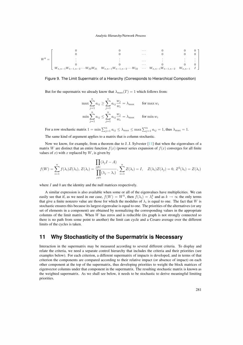
Analytic Hierarchy/Network Process
W k =
2666664
0 0 · · · 0 0 00 0 · · · 0 0 0...
... · · ·...
......
0 0 · · · 0 0 0Wn,n−1Wn−1,n−2 · · ·W32W21 Wn,n−1Wn−1,n−2 · · ·W32 · · · Wn,n−1Wn−1,n−2 Wn,n−1 I
3777775
Figure 9. The Limit Supermatrix of a Hierarchy (Corresponds to Hierarchical Composition)
But for the supermatrix we already know that λmax(T ) = 1 which follows from:
maxn∑
j=1
aij ≥n∑
j=1
aijwj
wi= λmax for max wi
minn∑
j=1
aij ≤n∑
j=1
aijwj
wi= λmax for min wi
For a row stochastic matrix 1 = min∑n
j=1 aij ≤ λmax ≤ max∑n
j=1 aij = 1, thus λmax = 1.
The same kind of argument applies to a matrix that is column stochastic.
Now we know, for example, from a theorem due to J. J. Sylvester [11] that when the eigenvalues of amatrix W are distinct that an entire function f(x) (power series expansion of f(x) converges for all finitevalues of x) with x replaced by W , is given by
f(W ) =n∑
i=1
f(λi)Z(λi), Z(λi) =
∏j �=i
(λjI −A)
∏j �=i
(λj − λi),
n∑i=1
Z(λi) = I, Z(λi)Z(λj) = 0, Z2(λi) = Z(λi)
where I and 0 are the identity and the null matrices respectively.
A similar expression is also available when some or all of the eigenvalues have multiplicities. We caneasily see that if, as we need in our case, f(W ) = W k, then f(λi) = λk
i and as k → ∞ the only termsthat give a finite nonzero value are those for which the modulus of λi is equal to one. The fact that W isstochastic ensures this because its largest eigenvalue is equal to one. The priorities of the alternatives (or anyset of elements in a component) are obtained by normalizing the corresponding values in the appropriatecolumns of the limit matrix. When W has zeros and is reducible (its graph is not strongly connected sothere is no path from some point to another) the limit can cycle and a Cesaro average over the differentlimits of the cycles is taken.
11 Why Stochasticity of the Supermatrix is Necessary
Interaction in the supermatrix may be measured according to several different criteria. To display andrelate the criteria, we need a separate control hierarchy that includes the criteria and their priorities (seeexamples below). For each criterion, a different supermatrix of impacts is developed, and in terms of thatcriterion the components are compared according to their relative impact (or absence of impact) on eachother component at the top of the supermatrix, thus developing priorities to weight the block matrices ofeigenvector columns under that component in the supermatrix. The resulting stochastic matrix is known asthe weighted supermatrix. As we shall see below, it needs to be stochastic to derive meaningful limitingpriorities.
281

Thomas L. Saaty
Before taking the limit, the supermatrix must first be reduced to a matrix, each of whose columnssums to unity, resulting in what is known as a column stochastic matrix. In general, a supermatrix is notstochastic. This is because its columns are made up of several eigenvectors whose entries in normalizedform sum to one and hence that column sums to the number of nonzero eigenvectors. In order to transformit to a stochastic matrix we need to compare its clusters, according to their impact on each other with respectto the general control criterion we have been considering and thus must do it several times for a decisionproblem, once for each control criterion, and for that criterion several matrices are needed. Each one is usedto compare the influence of all the clusters on a given cluster to which they are connected. This yields aneigenvector of influence of all the clusters on each cluster. Such a vector would have zero components whenthere is no influence. The priority of a component of such an eigenvector is used to weight all the elementsin the block of the supermatrix that corresponds to the elements of both the influencing and the influencedcluster. The result is a stochastic supermatrix. This is not a forced way to make the matrix stochastic. Itis natural. Why? Because the elements are compared among themselves and one needs information aboutthe importance of the clusters to which they belong, to determine their relative overall weight among allthe elements in the other clusters. Here is an example of why it is necessary to weight the priorities ofthe elements by those of their clusters: If one shouts into a room, “Ladies and Gentlemen, the president”,everyone is alerted and somewhat awed to expect to see the president of the United States because he is inthe news so often. But if the announcement is then followed by, "of the garbage collection association", thepriority immediately drops according to the importance of the group to which that president belongs. Wecannot avoid such a consideration.
The supermatrix of a hierarchy given above is already column stochastic and its clusters have equalweights. As a result, all the blocks of the matrix are multiplied by the same number. Thus the clustersdo not have to be weighted. Its limit matrix shown in Figure 9 has a form whose first entry in the bottomrow is the well-known hierarchic composition principle which gives the priorties of the alternatives in thebottom level with respect to the goal at the top. In this case, the limit supermatrix is obtained by raisingW to powers, but in this case the kth power (k ≥ n − 1) is sufficient to derive the principle of hierarchiccomposition in its (k, 1) position.
If the supermatrix is stochastic, the limiting priorities depend on its reducibility, primitivity, and cyclic-ity, with four cases to consider (see Table 14 below). Both acyclic cases are illustrated here. A matrix isreducible if on a permutation of rows and columns it can be put in the form
[B1 0B2 B3
]where B1 and B3
are square submatrices. Otherwise A is irreducible or non-decomposable. It is clear that the supermatrixof a hierarchy is reducible. Its principal eigenvalue λmax is a multiple eigenvalue. A matrix is primitive ifsome power of it is positive. Otherwise it is called imprimitive. A matrix has to be reducible in order forits powers to cycle which is best illustrated by the following example of successive powers of a matrix andhow they shift in an orderly cyclic way the nonzero entries from one power to the next:
W =
⎡⎣ 0 W12 0
0 0 W23
W31 0 0
⎤⎦ ; W 2 =
⎡⎣ 0 0 W12W23
W23W31 0 00 W31W12 0
⎤⎦
W 3 =
⎡⎣ W12W23W31 0 0
0 W23W31W12
0 0 W31W12W23
⎤⎦
W 3k =
⎡⎣ (W12W23W31)k 0 0
0 (W23W31W12)k 00 0 (W31W12W23)k
⎤⎦
W 3k+1 =
⎡⎣ 0 (W12W23W31)kW12 0
0 0 (W23W31W12)kW23
(W31W12W23)kW31 0 0
⎤⎦
282

Analytic Hierarchy/Network Process
W 3k+2 =
⎡⎣ 0 0 (W12W23W31)kW12W23
(W23W31W12)kW23W31 0 00 (W31W12W23)kW31W12 0
⎤⎦
Table 14. Characterization of W∞ in Terms of Eigenvalue MultiplicityAcyclic Cyclic
Irreducible λmax = 1 is a simple root C other eigenvalues with modulus = 1(they occur in conjugate pairs)
Reducible λmax = 1 is a multiple root C other eigenvalues with modulus = 1(they occur in conjugate pairs)
Let W be the stochastic matrix for which we wish to obtain f(W ) = W∞.
What we must do now is find a way to derive priorities for these four cases. We will consider the twocases when λmax = 1 is simple and then again when it is a multiple root.
Formally, because the right hand side in the decomposition formula above is a polynomial in W multi-plying both sides by W∞ each term on the right would become a constant multiplied by W∞ and the finaloutcome is also a constant multiplied by W∞. Because we are only interested in the relative values of theentries in W∞ we can ignore the constant and simply raise W to very large powers which the computerprogram SuperDecisions does in this case of distinct eigenvalues.
Next we consider the case where λmax = 1 is a multiple eigenvalue. For that case we have what isknown as the confluent form of Sylvester’s theorem:
f(W ) =k∑
j=1
T (λi) =k∑
j=1
1(mi − 1)!
dm−1
dλm−1f(λ)(λI −W )−1
∏ni=1(λ− λi)∏n
i=m+1(λ− λi)
∣∣∣∣λ−λ1
where k is the number of distinct roots and mi is the multiplicity of the root λi. However, as we showbelow, this too tells us that to obtain the limit priorities it is sufficient to raise W to arbitrarily large powerto obtain a satisfactory decimal approximation to W∞.
The only possible nonzero survivors as we raise the matrix to powers are those λ’s that are equal to oneor are roots of one. If the multiplicity of the largest real eigenvalue λmax = 1 is n1, then we have
W∞ = n1
d(n1−1)
dλ(n1−1)
[(λI −W )−1Δ(λ)
]Δ(n1)(λ)
∣∣∣∣∣∣λ=1
where one takes derivatives of the characteristic polynomial of the matrix W , and Δ(λ) = det(λI −W ) =λn + p1λ
n−1 + · · ·+ pn. Also (λI −W )−1 = F (λ)/Δ(λ) and
F (λ) = Wn−1 + (λ + p1)Wn−2 + (λ2 + pλ1 + p2)Wn−3 + · · ·+ (λn−1 + p1λn−2 + · · ·+ pn−1)I
is the adjoint of (λI −W ).
Now the right side is a polynomial in W . Again, if we multiply both sides by W∞, we would have onthe right a constant multiplied by W∞ which means that we can obtain W∞ by raising W to large powers.
For the cases of roots of one when λmax = 1 is a simple or a multiple root let us again formally see whathappens to our polynomial expressions on the right in both of Sylvester’s formulas as we now multiply bothon the left and on the right first by (W c)∞ obtaining one equation and then again by (W c+1)∞ obtaining
283

Thomas L. Saaty
another and so on c times, finally multiplying both sides by (W c+c−1)∞. We then sum these equations andtake their average on both sides. The left side of each of the equations reduces to W∞ and the average is1cW∞. On the right side the sum for each eigenvalue that is a root of unity is simply a constant times thesum (W c)∞+(W c+1)∞+ · · ·+(W c+c−1)∞. Also, because this sum is common to all the eigenvalues, itfactors out and their different constants sum to a new constant multiplied by (1/c). This is true whether oneis a simple or a multiple eigenvalue because the same process applies to accumulating its constants. In thevery end we simply have 1
c
[(W c)∞ + (W c+1)∞ + · · ·+ (W c+c−1)∞
]= 1
c (1+W +· · ·+W c−1)(W c)∞,c ≥ 2, which amounts to averaging over a cycle of length c obtained in raising W to infinite power. Thecyclicity c can be determined, among others, by noting the return of the form of the matrix of powers of Wto the original form of blocks of zero in W .
Caution: Some interesting things can happen in the limit supermatrix when it is reducible. For exampleif we have multiple goals in a hierarchy that are not connected to a higher goal, that is if we have multiplesources, we may have several limit vectors for the alternatives and these must be synthesized somehow togive a unique answer. To do that, the sources need to be connected to a higher goal and prioritized withrespect to it. Otherwise, the outcome would not be unique and we would obtain nothing that is meaningfulin a cooperative decision (but may be useful in a non-cooperative problem where the goals for example, aredifferent ways of facing an opponent). It is significant to note that a hierarchy always has a single sourcenode (the goal) and a single sink cluster (the alternatives), yet its supermatrix is reducible. Only when thesupermatrix is irreducible, and thus its graph is strongly connected with a path from any node or clusterto any other node or cluster, that the columns of the supermatrix would be identical. It is rare that thesupermatrix of a decision problem is irreducible. If the source clusters do not have sufficient interactionto serve as a single source, one could take the average of the alternatives relating to the several sources asif they are equally important to obtain a single overall outcome. As we have seen with the supermatrix ofa hierarchy in Figure 10, for sink nodes or clusters, at which arrows representing influence terminate andno arrows are directed outward from them, there needs to be a loop representing the identity matrix so thatwhen the supermatrix is raised to infinite powers, they receive values that are generally different from zero.For further emphasis of the latter observation, we work out briefly a useful example in the next section.
12 ANP Formulation of the Classic AHP School Example
We show below in Figure 10 the hierarchy, and in Figure 11 its corresponding supermatrix, and limitsupermatrix to obtain the priorities of three schools involved in a decision to choose the best one. Theyare precisely what one obtains by hierarchic composition using the AHP. The priorities of the criteria withrespect to the goal and those of the alternatives with respect to each criterion are clearly discernible in thesupermatrix itself. Note that there is an identity submatrix for the alternatives with respect to the alternativesin the lower right hand part of the matrix. The level of alternatives in a hierarchy is a sink cluster of nodesthat absorbs priorities but does not pass them on. This calls for using an identity submatrix for them in thesupermatrix.
13 Market Share Example
13.1 An ANP Network with a Single Control Criterion - Market Share
A market share estimation model is structured as a network of clusters and nodes. The object is to try todetermine the relative market share of competitors in a particular business, or endeavor, by considering whataffects market share in that business and introduce them as clusters, nodes and influence links in a network.The decision alternatives are the competitors and the synthesized results are their relative dominance. Therelative dominance results can then be compared against some outside measure such as dollars. If dollar
284

Analytic Hierarchy/Network Process
Figure 10. The School Choice Hierarchy
Figure 11. The Limit Supermatrix of the School Choice Hierarchy shows same Result as Hierar-chic Composition
income is the measure being used, the incomes of the competitors must be normalized to get it in terms ofrelative market share.
The clusters might include customers, service, economics, advertising, and the quality of goods. Thecustomers’ cluster might then include nodes for the age groups of the people that buy from the business:teenagers, 20–33 year olds, 34–55 year olds, 55–70 year olds, and over 70. The advertising cluster mightinclude newspapers, TV, Radio, and Fliers. After all the nodes are created one starts by picking a node
285

Thomas L. Saaty
and linking it to the other nodes in the model that influence it. The “children” nodes will then be pairwisecompared with respect to that node as a “parent” node. An arrow will automatically appear going from thecluster the parent node cluster to the cluster with its children nodes. When a node is linked to nodes in itsown cluster, the arrow becomes a loop on that cluster and we say there is inner dependence.
The linked nodes in a given cluster are pairwise compared for their influence on the node they arelinked from (the parent node) to determine the priority of their influence on the parent node. Comparisonsare made as to which is more important to the parent node in capturing “market share”. These priorities arethen entered in the supermatrix for the network.
The clusters are also pairwise compared to establish their importance with respect to each cluster theyare linked from, and the resulting matrix of numbers is used to weight the corresponding blocks of theoriginal unweighted supermatrix to obtain the weighted supermatrix. This matrix is then raised to powersuntil it converges to yield the limit supermatrix. The relative values for the companies are obtained fromthe columns of the limit supermatrix that in this case are all the same because the matrix is irreducible.Normalizing these numbers yields the relative market share.
If comparison data in terms of sales in dollars, or number of members, or some other known measuresare available, one can use these relative values to validate the outcome. The AHP/ANP has a compatibilitymetric to determine how close the ANP result is to the known measure. It involves taking the Hadamardproduct of the matrix of ratios of the ANP outcome and the transpose of the matrix of ratios of the actualoutcome summing all the coefficients and dividing by n2. The requirement is that the value should be closeto 1.
We will give two examples of market share estimation showing details of the process in the first exampleand showing only the models and results in the second example.
13.2 Estimating The Relative Market Share Of Walmart, Kmart And TargetThe network for the ANP model shown in Figure 12 well describes the influences that determine the marketshare of these companies. We will not dwell on describing the clusters and nodes.
13.3 The Unweighted SupermatrixThe unweighted supermatrix is constructed from the priorities derived from the different pairwise compar-isons. The column for a node contains the priorities of all the nodes that have been pairwise compared withrespect to it and influence it with respect to the control criterion “market share”. The supermatrix for thenetwork in Figure 12 is shown in two parts in Tables 15 and 16.
13.4 The Cluster MatrixThe cluster themselves must be compared to establish their relative importance and use it to weight thecorresponding blocks of the supermatrix to make it column stochastic. A cluster impacts another clusterwhen it is linked from it, that is, when at least one node in the source cluster is linked to nodes in thetarget cluster. The clusters linked from the source cluster are pairwise compared for the importance of theirimpact on it with respect to market share, resulting in the column of priorities for that cluster in the clustermatrix. The process is repeated for each cluster in the network to obtain the matrix shown in Table 17. Aninterpretation of the priorities in the first column is that Merchandise (0.442) and Locations (0.276) havethe most impact on Alternatives, the three competitors.
13.5 Weighted SupermatrixThe weighted supermatrix shown in Tables 18 and 19 is obtained by multiplying each entry in a block ofthe component at the top of the supermatrix by the priority of influence of the component on the left from
286

Analytic Hierarchy/Network Process
Figure 12. The Clusters and Nodes of a Model to Estimate the Relative Market Share of Walmart,Kmart and Target
the cluster matrix in Table 17. For example, the first entry, 0.137, in Table 17 is used to multiply each ofthe nine entries in the block (Alternatives, Alternatives) in the unweighted supermatrix shown in Tables 15and 16. This gives the entries for the Alternatives, Alternatives component in the weighted supermatrix ofTable 18. Each column in the weighted supermatrix has a sum of 1, and thus the matrix is stochastic.
13.6 Limit Supermatrix
The limit supermatrix shown in Tables 20 and 21 is obtained from the weighted supermatrix, as we saidabove. To obtain the final answer we form the Cesaro average of the progression of successive limit vectors.
13.7 Synthesized Results
The relative market shares of the alternatives, 0.599, 0.248 and 0.154 are displayed as synthesized results inthe SuperDecisions Program, shown in the middle column of Table 22. They are obtained by normalizingthe values for Walmart, Kmart and Target: 0.057, 0.024 and 0.015, taken from the limit supermatrix. TheIdealized values are obtained from the Normalized values by dividing each value by the largest value in thatcolumn.
In the AHP/ANP the question arises as to how close one priority vector is to another priority vector ofrelative measurement. When two vectors are close, we say they are compatible. The question is how tomeasure compatibility in a meaningful way. It turns out that consistency and compatibility can be related ina useful way. Our development of a compatibility measure uses the idea of the Hadamard or element-wiseproduct of two matrices.
287

Thomas L. Saaty
Table 15. The Unweighted Supermatrix - Part I
1A
ltern
ativ
es2
Adv
ertis
ing
3L
ocat
ions
1W
al-
mar
t2 K
mar
t3
Tar-
get
1T
V2
Prin
tM
edia
3R
a-di
o
4D
i-re
ctM
ail
1 Urb
an2
Sub-
urba
n3
Ru-
ral
1W
alm
art
0.00
00.
833
0.83
30.
687
0.54
00.
634
0.66
10.
614
0.65
20.
683
1A
ltern
ativ
es2
Km
art
0.75
00.
000
0.16
70.
186
0.29
70.
174
0.20
80.
268
0.23
50.
200
3Ta
rget
0.25
00.
167
0.00
00.
127
0.16
30.
192
0.13
10.
117
0.11
30.
117
1T
V0.
553
0.17
60.
188
0.00
00.
000
0.00
00.
000
0.28
80.
543
0.55
82
Adv
ertis
ing
2Pr
intM
edia
0.20
20.
349
0.42
80.
750
0.00
00.
800
0.00
00.
381
0.23
10.
175
3R
adio
0.06
20.
056
0.05
50.
000
0.00
00.
000
0.00
00.
059
0.05
30.
048
4D
irec
tMai
l0.
183
0.42
00.
330
0.25
00.
000
0.20
00.
000
0.27
30.
173
0.21
91
Urb
an0.
114
0.08
40.
086
0.44
30.
126
0.08
00.
099
0.00
00.
000
0.00
03
Loc
atio
ns2
Subu
rban
0.40
50.
444
0.62
80.
387
0.41
60.
609
0.53
70.
000
0.00
00.
000
3R
ural
0.48
10.
472
0.28
50.
169
0.45
80.
311
0.36
40.
000
0.00
00.
000
1W
hite
Col
lar
0.14
10.
114
0.20
80.
165
0.15
50.
116
0.12
00.
078
0.19
80.
092
4C
ust.G
roup
s2
Blu
eC
olla
r0.
217
0.21
40.
117
0.16
50.
155
0.19
80.
203
0.22
30.
116
0.22
43
Fam
ilies
0.57
90.
623
0.62
00.
621
0.64
60.
641
0.63
50.
656
0.64
10.
645
4Te
enag
ers
0.06
30.
049
0.05
50.
048
0.04
30.
045
0.04
10.
043
0.04
50.
038
1L
owC
ost
0.36
20.
333
0.16
80.
000
0.00
00.
000
0.00
00.
000
0.00
00.
000
5M
erch
andi
se2
Qua
lity
0.26
10.
140
0.48
40.
000
0.00
00.
000
0.00
00.
000
0.00
00.
000
3V
arie
ty0.
377
0.52
80.
349
0.00
00.
000
0.00
00.
000
0.00
00.
000
0.00
01
Lig
htin
g0.
000
0.00
00.
000
0.00
00.
000
0.00
00.
000
0.00
00.
000
0.00
02
Org
aniz
atio
n0.
000
0.00
00.
000
0.00
00.
000
0.00
00.
000
0.00
00.
000
0.00
06
Cha
ract
eris
tic3
Cle
anlin
ess
0.00
00.
000
0.00
00.
000
0.00
00.
000
0.00
00.
000
0.00
00.
000
4E
mpl
oyee
s0.
000
0.00
00.
000
0.00
00.
000
0.00
00.
000
0.00
00.
000
0.00
05
Park
ing
0.00
00.
000
0.00
00.
000
0.00
00.
000
0.00
00.
000
0.00
00.
000
288

Analytic Hierarchy/Network Process
Table 16. The Unweighted Supermatrix - Part II
4C
usto
mer
Gro
ups
5M
erch
andi
se6
Cha
ract
eris
tics
ofSt
ore
1 Whi
teC
ol-
lar
2 Blu
eC
ol-
lar
3 Fam
i-lie
s
4 Teen
s
1 Low
Cos
t
2 Qua
l-ity
3V
a-ri
ety
1 Lig
ht’
ng
2O
r-ga
ni-
zatio
n
3 Cle
an
4E
m-
ploy
-ee
s
5 Park
1W
alm
art
0.6
37
0.6
61
0.6
30
0.6
91
0.6
61
0.6
14
0.6
48
0.6
67
0.6
55
0.5
70
0.6
44
0.5
58
1A
ltern
ativ
es2
Km
art
0.1
05
0.2
08
0.2
18
0.1
49
0.2
08
0.1
17
0.1
22
0.1
11
0.0
95
0.0
97
0.0
85
0.1
22
3Ta
rget
0.2
58
0.1
31
0.1
51
0.1
60
0.1
31
0.2
68
0.2
30
0.2
22
0.2
50
0.3
33
0.2
71
0.3
20
1T
V0.3
23
0.5
10
0.5
08
0.6
34
0.0
00
0.0
00
0.0
00
0.0
00
0.0
00
0.0
00
0.0
00
0.0
00
2A
dver
tisin
g2
Prin
tMed
.0.2
14
0.2
21
0.2
70
0.1
70
0.0
00
0.0
00
0.0
00
0.0
00
0.0
00
0.0
00
0.0
00
0.0
00
3R
adio
0.0
59
0.0
63
0.0
49
0.0
96
0.0
00
0.0
00
0.0
00
0.0
00
0.0
00
0.0
00
0.0
00
0.0
00
4D
irec
tMai
l0.4
04
0.2
06
0.1
73
0.1
00
0.0
00
0.0
00
0.0
00
0.0
00
0.0
00
0.0
00
0.0
00
0.0
00
1U
rban
0.1
67
0.0
94
0.0
96
0.1
09
0.2
68
0.1
05
0.0
94
0.1
00
0.0
91
0.0
91
0.1
11
0.0
67
3L
ocat
ions
2Su
burb
an0.8
33
0.2
80
0.3
08
0.3
09
0.1
17
0.6
05
0.6
27
0.4
33
0.4
55
0.4
55
0.4
44
0.2
93
3R
ural
0.0
00
0.6
27
0.5
96
0.5
82
0.6
14
0.2
91
0.2
80
0.4
66
0.4
55
0.4
55
0.4
44
0.6
41
1W
hite
Col
lar
0.0
00
0.0
00
0.2
79
0.0
85
0.0
51
0.2
22
0.1
65
0.3
83
0.1
87
0.2
42
0.1
65
0.0
00
4C
usto
mer
s2
Blu
eC
olla
r0.0
00
0.0
00
0.6
49
0.1
77
0.1
12
0.1
59
0.1
65
0.3
83
0.1
87
0.2
08
0.1
65
0.0
00
3Fa
mili
es0.8
57
0.8
57
0.0
00
0.7
37
0.6
18
0.5
66
0.6
21
0.1
85
0.5
83
0.4
94
0.6
21
0.0
00
4Te
enag
ers
0.1
43
0.1
43
0.0
72
0.0
00
0.2
19
0.0
53
0.0
48
0.0
48
0.0
43
0.0
56
0.0
48
0.0
00
1Low
Cos
t0.0
00
0.0
00
0.0
00
0.0
00
0.0
00
0.8
00
0.8
00
0.0
00
0.0
00
0.0
00
0.0
00
0.0
00
5M
erch
andi
se2
Qua
lity
0.0
00
0.0
00
0.0
00
0.0
00
0.7
50
0.0
00
0.2
00
0.0
00
0.0
00
0.0
00
0.0
00
0.0
00
3V
arie
ty0.0
00
0.0
00
0.0
00
0.0
00
0.2
50
0.2
00
0.0
00
0.0
00
1.0
00
0.0
00
0.0
00
0.0
00
1L
ight
ing
0.0
00
0.0
00
0.0
00
0.0
00
0.0
00
0.0
00
0.0
00
0.0
00
0.1
69
0.1
21
0.0
00
0.2
50
2O
rgan
izat
ion
0.0
00
0.0
00
0.0
00
0.0
00
0.0
00
0.0
00
0.0
00
0.2
51
0.0
00
0.5
75
0.2
00
0.7
50
6C
hara
cter
istic
s3
Cle
anlin
ess
0.0
00
0.0
00
0.0
00
0.0
00
0.0
00
0.0
00
0.0
00
0.6
73
0.4
69
0.0
00
0.8
00
0.0
00
4E
mpl
oyee
0.0
00
0.0
00
0.0
00
0.0
00
0.0
00
0.0
00
0.0
00
0.0
00
0.3
08
0.3
04
0.0
00
0.0
00
5Pa
rkin
g0.0
00
0.0
00
0.0
00
0.0
00
0.0
00
0.0
00
0.0
00
0.0
75
0.0
55
0.0
00
0.0
00
0.0
00
289

Thomas L. Saaty
Table 17. The Cluster Matrix
1 2 3 4 5 6
Alternatives Advertising LocationsCustomerGroups
MerchandiseCharacteristicsof Store
1 Alternatives 0.137 0.174 0.094 0.057 0.049 0.037
2 Advertising 0.091 0.220 0.280 0.234 0.000 0.000
3 Locations 0.276 0.176 0.000 0.169 0.102 0.112
4 Customer Groups 0.054 0.429 0.627 0.540 0.252 0.441
5 Merchandise 0.442 0.000 0.000 0.000 0.596 0.316
6 Characteristics of Store 0.000 0.000 0.000 0.000 0.000 0.094
13.8 Compatibility IndexLet us show first that the priority vector w = (w1, . . . , wn) is completely compatible with itself. Thus weform the matrix of all possible ratios W = (wij) = (wi/wj) from this vector. This matrix is reciprocal,that is wji = 1/wij . The Hadamard product of a reciprocal matrix W and its transpose WT is given by:
W ◦WT =
⎡⎢⎣
w1w1
· · · w1wn
.... . .
...wn
w1· · · wn
wn
⎤⎥⎦◦⎡⎢⎣
w1w1
· · · wn
w1...
. . ....
w1wn
· · · wn
wn
⎤⎥⎦ =
⎡⎢⎣
1 · · · 1...
. . ....
1 · · · 1
⎤⎥⎦ =
⎡⎢⎣
1...1
⎤⎥⎦ [ 1 · · · 1
]= eeT
The sum of the elements of a matrix A can be written as eT Ae. In particular we have eT A◦AT e = n2 forthe sum of the elements of the Hadamard product of a matrix and its transpose. The index of compatibilityis the sum resulting from the Hadamard product divided by n2. Thus a vector is completely compatiblewith itself as n2
n2 = 1. Now we have an idea of how to define a measure of compatibility for two matrices Aand B. It is given by 1
n2 eT A ◦ BT e. Note that a reciprocal matrix of judgments that is inconsistent is notitself a matrix of ratios from a given vector. However, such a matrix has a principal eigenvector and thuswe speak of the compatibility of the matrix of judgments and the matrix formed from ratios of the principaleigenvector. We have the following theorem for a reciprocal matrix of judgments and the matrix W of theratios of its principal eigenvector:
Theorem 1.1n2
eT A ◦WT e =λmax
n
PROOF. From Aw = λmaxw we have∑n
j=1 aijwj = λmaxwi and
1n2
eT A ◦WT e =1n2
n∑i=1
n∑j=1
aijwj
wi=
λmax
n
�We want this ratio to be close to one or in general not much more than 1.01 and be less than this value
for small size matrices. It is in accord with the idea that a 10% deviation is at the upper end of acceptability.
13.9 Actual Relative Market Share Based on SalesThe object was to estimate the market share of Walmart, Kmart, and Target. The normalized results fromthe model were compared with sales shown in Table 22 as reported in the Discount Store News of July 13,1998, p. 77, of $58, $27.5 and $20.3 billions of dollars respectively. Normalizing the dollar amounts showstheir actual relative market shares to be 54.8, 25.9 and 19.2. The relative market share from the model
290

Analytic Hierarchy/Network Process
Table 18. The Weighted Supermatrix - Part I
1A
ltern
ativ
es2
Adv
ertis
ing
3L
ocat
ions
1W
al-
mar
t2 K
mar
t3
Tar-
get
1T
V2
Prin
tM
edia
3R
a-di
o
4D
i-re
ctM
ail
1 Urb
an2
Sub-
urba
n3
Ru-
ral
1W
alm
art
0.00
00.
114
0.11
40.
120
0.12
10.
110
0.14
80.
058
0.06
10.
064
1A
ltern
ativ
es2
Km
art
0.10
30.
000
0.02
30.
033
0.06
60.
030
0.04
70.
025
0.02
20.
019
3Ta
rget
0.03
40.
023
0.00
00.
022
0.03
70.
033
0.02
90.
011
0.01
10.
011
1T
V0.
050
0.01
60.
017
0.00
00.
000
0.00
00.
000
0.08
00.
152
0.15
62
Adv
ertis
ing
2Pr
intM
edia
0.01
80.
032
0.03
90.
165
0.00
00.
176
0.00
00.
106
0.06
40.
049
3R
adio
0.00
60.
005
0.00
50.
000
0.00
00.
000
0.00
00.
016
0.01
50.
014
4D
irec
tMai
l0.
017
0.03
80.
030
0.05
50.
000
0.04
40.
000
0.07
60.
048
0.06
11
Urb
an0.
031
0.02
30.
024
0.07
80.
028
0.01
40.
022
0.00
00.
000
0.00
03
Loc
atio
ns2
Subu
rban
0.11
20.
123
0.17
40.
068
0.09
40.
107
0.12
10.
000
0.00
00.
000
3R
ural
0.13
30.
130
0.07
90.
030
0.10
30.
055
0.08
20.
000
0.00
00.
000
1W
hite
Col
lar
0.00
80.
006
0.01
10.
071
0.08
60.
050
0.06
60.
049
0.12
40.
058
4C
ust.G
roup
s2
Blu
eC
olla
r0.
012
0.01
10.
006
0.07
10.
086
0.08
50.
112
0.14
00.
073
0.14
13
Fam
ilies
0.03
10.
033
0.03
30.
267
0.35
60.
275
0.35
00.
411
0.40
20.
404
4Te
enag
ers
0.00
30.
003
0.00
30.
021
0.02
40.
019
0.02
30.
027
0.02
80.
024
1L
owC
ost
0.16
00.
147
0.07
40.
000
0.00
00.
000
0.00
00.
000
0.00
00.
000
5M
erch
andi
se2
Qua
lity
0.11
50.
062
0.21
40.
000
0.00
00.
000
0.00
00.
000
0.00
00.
000
3V
arie
ty0.
166
0.23
30.
154
0.00
00.
000
0.00
00.
000
0.00
00.
000
0.00
01
Lig
htin
g0.
000
0.00
00.
000
0.00
00.
000
0.00
00.
000
0.00
00.
000
0.00
02
Org
aniz
atio
n0.
000
0.00
00.
000
0.00
00.
000
0.00
00.
000
0.00
00.
000
0.00
06
Cha
ract
eris
tic3
Cle
anlin
ess
0.00
00.
000
0.00
00.
000
0.00
00.
000
0.00
00.
000
0.00
00.
000
4E
mpl
oyee
s0.
000
0.00
00.
000
0.00
00.
000
0.00
00.
000
0.00
00.
000
0.00
05
Park
ing
0.00
00.
000
0.00
00.
000
0.00
00.
000
0.00
00.
000
0.00
00.
000
291

Thomas L. Saaty
Table 19. The Weighted Supermatrix - Part II
4C
usto
mer
Gro
ups
5M
erch
andi
se6
Cha
ract
eris
tics
ofSt
ore
1 Whi
teC
ol-
lar
2 Blu
eC
ol-
lar
3 Fam
i-lie
s
4 Teen
s
1 Low
Cos
t
2 Qua
l-ity
3V
a-ri
ety
1 Lig
ht’
ng
2O
r-ga
ni-
zatio
n
3 Cle
an
4E
m-
ploy
-ee
s
5 Park
1W
alm
art
0.0
36
0.0
38
0.0
36
0.0
40
0.0
33
0.0
30
0.0
32
0.0
36
0.0
24
0.0
31
0.0
35
0.0
86
1Alte
rnat
ives
2K
mar
t0.0
06
0.0
12
0.0
12
0.0
09
0.0
10
0.0
06
0.0
06
0.0
06
0.0
04
0.0
05
0.0
05
0.0
19
3Ta
rget
0.0
15
0.0
07
0.0
09
0.0
09
0.0
06
0.0
13
0.0
11
0.0
12
0.0
09
0.0
18
0.0
15
0.0
49
1T
V0.0
76
0.1
19
0.1
19
0.1
48
0.0
00
0.0
00
0.0
00
0.0
00
0.0
00
0.0
00
0.0
00
0.0
00
2A
dver
tisin
g2
Prin
tMed
.0.0
50
0.0
52
0.0
63
0.0
40
0.0
00
0.0
00
0.0
00
0.0
00
0.0
00
0.0
00
0.0
00
0.0
00
3R
adio
0.0
14
0.0
15
0.0
12
0.0
23
0.0
00
0.0
00
0.0
00
0.0
00
0.0
00
0.0
00
0.0
00
0.0
00
4D
irec
tMai
l0.0
95
0.0
48
0.0
40
0.0
23
0.0
00
0.0
00
0.0
00
0.0
00
0.0
00
0.0
00
0.0
00
0.0
00
1U
rban
0.0
28
0.0
16
0.0
16
0.0
18
0.0
27
0.0
11
0.0
10
0.0
16
0.0
10
0.0
15
0.0
18
0.0
31
3L
ocat
ions
2Su
burb
an0.1
41
0.0
47
0.0
52
0.0
52
0.0
12
0.0
62
0.0
64
0.0
71
0.0
51
0.0
74
0.0
73
0.1
35
3R
ural
0.0
00
0.1
06
0.1
01
0.0
98
0.0
63
0.0
30
0.0
29
0.0
76
0.0
51
0.0
74
0.0
73
0.2
95
1W
hite
Col
lar
0.0
00
0.0
00
0.1
51
0.0
46
0.0
13
0.0
56
0.0
42
0.2
47
0.0
82
0.1
56
0.1
07
0.0
00
4Cus
tom
ers
2B
lue
Col
lar
0.0
00
0.0
00
0.3
50
0.0
96
0.0
28
0.0
40
0.0
42
0.2
47
0.0
82
0.1
34
0.1
07
0.0
00
3Fa
mili
es0.4
63
0.4
63
0.0
00
0.3
98
0.1
56
0.1
43
0.1
57
0.1
19
0.2
57
0.3
18
0.4
00
0.0
00
4Te
enag
ers
0.0
77
0.0
77
0.0
39
0.0
00
0.0
55
0.0
13
0.0
12
0.0
31
0.0
19
0.0
36
0.0
31
0.0
00
1L
owC
ost
0.0
00
0.0
00
0.0
00
0.0
00
0.0
00
0.4
77
0.4
77
0.0
00
0.0
00
0.0
00
0.0
00
0.0
00
5M
erch
andi
se2
Qua
lity
0.0
00
0.0
00
0.0
00
0.0
00
0.4
47
0.0
00
0.1
19
0.0
00
0.0
00
0.0
00
0.0
00
0.0
00
3V
arie
ty0.0
00
0.0
00
0.0
00
0.0
00
0.1
49
0.1
19
0.0
00
0.0
00
0.3
16
0.0
00
0.0
00
0.0
00
1L
ight
ing
0.0
00
0.0
00
0.0
00
0.0
00
0.0
00
0.0
00
0.0
00
0.0
00
0.0
16
0.0
17
0.0
00
0.0
97
2O
rgan
izat
ion
0.0
00
0.0
00
0.0
00
0.0
00
0.0
00
0.0
00
0.0
00
0.0
35
0.0
00
0.0
79
0.0
27
0.2
90
6C
hara
cter
istic
s3
Cle
anlin
ess
0.0
00
0.0
00
0.0
00
0.0
00
0.0
00
0.0
00
0.0
00
0.0
92
0.0
44
0.0
00
0.1
10
0.0
00
4E
mpl
oyee
0.0
00
0.0
00
0.0
00
0.0
00
0.0
00
0.0
00
0.0
00
0.0
00
0.0
29
0.0
42
0.0
00
0.0
00
5Pa
rkin
g0.0
00
0.0
00
0.0
00
0.0
00
0.0
00
0.0
00
0.0
00
0.0
10
0.0
05
0.0
00
0.0
00
0.0
00
292

Analytic Hierarchy/Network Process
Table 20. The Limit Supermatrix - Part I
1A
ltern
ativ
es2
Adv
ertis
ing
3L
ocat
ions
1W
al-
mar
t2 K
mar
t3
Tar-
get
1T
V2
Prin
tM
edia
3R
a-di
o
4D
i-re
ctM
ail
1 Urb
an2
Sub-
urba
n3
Ru-
ral
1W
alm
art
0.05
70.
057
0.05
70.
057
0.05
70.
057
0.05
70.
057
0.05
70.
057
1A
ltern
ativ
es2
Km
art
0.02
40.
024
0.02
40.
024
0.02
40.
024
0.02
40.
024
0.02
40.
024
3Ta
rget
0.01
50.
015
0.01
50.
015
0.01
50.
015
0.01
50.
015
0.01
50.
015
1T
V0.
079
0.07
90.
079
0.07
90.
079
0.07
90.
079
0.07
90.
079
0.07
92
Adv
ertis
ing
2Pr
intM
edia
0.05
30.
053
0.05
30.
053
0.05
30.
053
0.05
30.
053
0.05
30.
053
3R
adio
0.00
90.
009
0.00
90.
009
0.00
90.
009
0.00
90.
009
0.00
90.
009
4D
irec
tMai
l0.
039
0.03
90.
039
0.03
90.
039
0.03
90.
039
0.03
90.
039
0.03
91
Urb
an0.
022
0.02
20.
022
0.02
20.
022
0.02
20.
022
0.02
20.
022
0.02
23
Loc
atio
ns2
Subu
rban
0.06
20.
062
0.06
20.
062
0.06
20.
062
0.06
20.
062
0.06
20.
062
3R
ural
0.06
90.
069
0.06
90.
069
0.06
90.
069
0.06
90.
069
0.06
90.
069
1W
hite
Col
lar
0.06
80.
068
0.06
80.
068
0.06
80.
068
0.06
80.
068
0.06
80.
068
4C
ust.G
roup
s2
Blu
eC
olla
r0.
125
0.12
50.
125
0.12
50.
125
0.12
50.
125
0.12
50.
125
0.12
53
Fam
ilies
0.24
00.
240
0.24
00.
240
0.24
00.
240
0.24
00.
240
0.24
00.
240
4Te
enag
ers
0.03
60.
036
0.03
60.
036
0.03
60.
036
0.03
60.
036
0.03
60.
036
1L
owC
ost
0.04
30.
043
0.04
30.
043
0.04
30.
043
0.04
30.
043
0.04
30.
043
5M
erch
andi
se2
Qua
lity
0.03
40.
034
0.03
40.
034
0.03
40.
034
0.03
40.
034
0.03
40.
034
3V
arie
ty0.
028
0.02
80.
028
0.02
80.
028
0.02
80.
028
0.02
80.
028
0.02
81
Lig
htin
g0.
000
0.00
00.
000
0.00
00.
000
0.00
00.
000
0.00
00.
000
0.00
02
Org
aniz
atio
n0.
000
0.00
00.
000
0.00
00.
000
0.00
00.
000
0.00
00.
000
0.00
06
Cha
ract
eris
tic3
Cle
anlin
ess
0.00
00.
000
0.00
00.
000
0.00
00.
000
0.00
00.
000
0.00
00.
000
4E
mpl
oyee
s0.
000
0.00
00.
000
0.00
00.
000
0.00
00.
000
0.00
00.
000
0.00
05
Park
ing
0.00
00.
000
0.00
00.
000
0.00
00.
000
0.00
00.
000
0.00
00.
000
293

Thomas L. Saaty
Table 21. The Limit Supermatrix - Part II
4C
usto
mer
Gro
ups
5M
erch
andi
se6
Cha
ract
eris
tics
ofSt
ore
1 Whi
teC
ol-
lar
2 Blu
eC
ol-
lar
3 Fam
i-lie
s
4 Teen
s
1 Low
Cos
t
2 Qua
l-ity
3V
a-ri
ety
1 Lig
ht’
ng
2O
r-ga
ni-
zatio
n
3 Cle
an
4E
m-
ploy
-ee
s
5 Park
1W
alm
art
0.0
57
0.0
57
0.0
57
0.0
57
0.0
57
0.0
57
0.0
57
0.0
57
0.0
57
0.0
57
0.0
57
0.0
57
1Alte
rnat
ives
2K
mar
t0.0
24
0.0
24
0.0
24
0.0
24
0.0
24
0.0
24
0.0
24
0.0
24
0.0
24
0.0
24
0.0
24
0.0
24
3Ta
rget
0.0
15
0.0
15
0.0
15
0.0
15
0.0
15
0.0
15
0.0
15
0.0
15
0.0
15
0.0
15
0.0
15
0.0
15
1T
V0.0
79
0.0
79
0.0
79
0.0
79
0.0
79
0.0
79
0.0
79
0.0
79
0.0
79
0.0
79
0.0
79
0.0
79
2A
dver
tisin
g2
Prin
tMed
.0.0
53
0.0
53
0.0
53
0.0
53
0.0
53
0.0
53
0.0
53
0.0
53
0.0
53
0.0
53
0.0
53
0.0
53
3R
adio
0.0
09
0.0
09
0.0
09
0.0
09
0.0
09
0.0
09
0.0
09
0.0
09
0.0
09
0.0
09
0.0
09
0.0
09
4D
irec
tMai
l0.0
39
0.0
39
0.0
39
0.0
39
0.0
39
0.0
39
0.0
39
0.0
39
0.0
39
0.0
39
0.0
39
0.0
39
1U
rban
0.0
22
0.0
22
0.0
22
0.0
22
0.0
22
0.0
22
0.0
22
0.0
22
0.0
22
0.0
22
0.0
22
0.0
22
3L
ocat
ions
2Su
burb
an0.0
62
0.0
62
0.0
62
0.0
62
0.0
62
0.0
62
0.0
62
0.0
62
0.0
62
0.0
62
0.0
62
0.0
62
3R
ural
0.0
69
0.0
69
0.0
69
0.0
69
0.0
69
0.0
69
0.0
69
0.0
69
0.0
69
0.0
69
0.0
69
0.0
69
1W
hite
Col
lar
0.0
68
0.0
68
0.0
68
0.0
68
0.0
68
0.0
68
0.0
68
0.0
68
0.0
68
0.0
68
0.0
68
0.0
68
4Cus
tom
ers
2B
lue
Col
lar
0.1
25
0.1
25
0.1
25
0.1
25
0.1
25
0.1
25
0.1
25
0.1
25
0.1
25
0.1
25
0.1
25
0.1
25
3Fa
mili
es0.2
40
0.2
40
0.2
40
0.2
40
0.2
40
0.2
40
0.2
40
0.2
40
0.2
40
0.2
40
0.2
40
0.2
40
4Te
enag
ers
0.0
36
0.0
36
0.0
36
0.0
36
0.0
36
0.0
36
0.0
36
0.0
36
0.0
36
0.0
36
0.0
36
0.0
36
1L
owC
ost
0.0
43
0.0
43
0.0
43
0.0
43
0.0
43
0.0
43
0.0
43
0.0
43
0.0
43
0.0
43
0.0
43
0.0
43
5Mer
chan
dise
2Q
ualit
y0.0
34
0.0
34
0.0
34
0.0
34
0.0
34
0.0
34
0.0
34
0.0
34
0.0
34
0.0
34
0.0
34
0.0
34
3V
arie
ty0.0
28
0.0
28
0.0
28
0.0
28
0.0
28
0.0
28
0.0
28
0.0
28
0.0
28
0.0
28
0.0
28
0.0
28
1L
ight
ing
0.0
00
0.0
00
0.0
00
0.0
00
0.0
00
0.0
00
0.0
00
0.0
00
0.0
00
0.0
00
0.0
00
0.0
00
2O
rgan
izat
ion
0.0
00
0.0
00
0.0
00
0.0
00
0.0
00
0.0
00
0.0
00
0.0
00
0.0
00
0.0
00
0.0
00
0.0
00
6C
hara
cter
istic
s3
Cle
anlin
ess
0.0
00
0.0
00
0.0
00
0.0
00
0.0
00
0.0
00
0.0
00
0.0
00
0.0
00
0.0
00
0.0
00
0.0
00
4E
mpl
oyee
0.0
00
0.0
00
0.0
00
0.0
00
0.0
00
0.0
00
0.0
00
0.0
00
0.0
00
0.0
00
0.0
00
0.0
00
5Pa
rkin
g0.0
00
0.0
00
0.0
00
0.0
00
0.0
00
0.0
00
0.0
00
0.0
00
0.0
00
0.0
00
0.0
00
0.0
00
294
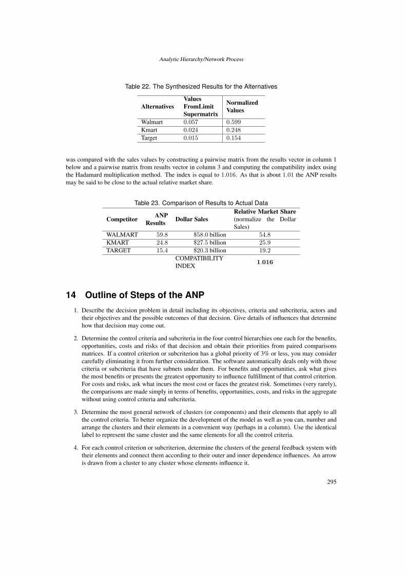
Analytic Hierarchy/Network Process
Table 22. The Synthesized Results for the Alternatives
AlternativesValuesFromLimitSupermatrix
NormalizedValues
Walmart 0.057 0.599Kmart 0.024 0.248Target 0.015 0.154
was compared with the sales values by constructing a pairwise matrix from the results vector in column 1below and a pairwise matrix from results vector in column 3 and computing the compatibility index usingthe Hadamard multiplication method. The index is equal to 1.016. As that is about 1.01 the ANP resultsmay be said to be close to the actual relative market share.
Table 23. Comparison of Results to Actual Data
Competitor ANPResults Dollar Sales
Relative Market Share(normalize the DollarSales)
WALMART 59.8 $58.0 billion 54.8KMART 24.8 $27.5 billion 25.9TARGET 15.4 $20.3 billion 19.2
COMPATIBILITYINDEX 1.016
14 Outline of Steps of the ANP1. Describe the decision problem in detail including its objectives, criteria and subcriteria, actors and
their objectives and the possible outcomes of that decision. Give details of influences that determinehow that decision may come out.
2. Determine the control criteria and subcriteria in the four control hierarchies one each for the benefits,opportunities, costs and risks of that decision and obtain their priorities from paired comparisonsmatrices. If a control criterion or subcriterion has a global priority of 3% or less, you may considercarefully eliminating it from further consideration. The software automatically deals only with thosecriteria or subcriteria that have subnets under them. For benefits and opportunities, ask what givesthe most benefits or presents the greatest opportunity to influence fulfillment of that control criterion.For costs and risks, ask what incurs the most cost or faces the greatest risk. Sometimes (very rarely),the comparisons are made simply in terms of benefits, opportunities, costs, and risks in the aggregatewithout using control criteria and subcriteria.
3. Determine the most general network of clusters (or components) and their elements that apply to allthe control criteria. To better organize the development of the model as well as you can, number andarrange the clusters and their elements in a convenient way (perhaps in a column). Use the identicallabel to represent the same cluster and the same elements for all the control criteria.
4. For each control criterion or subcriterion, determine the clusters of the general feedback system withtheir elements and connect them according to their outer and inner dependence influences. An arrowis drawn from a cluster to any cluster whose elements influence it.
295

Thomas L. Saaty
5. Determine the approach you want to follow in the analysis of each cluster or element, influencing(the preferred approach) other clusters and elements with respect to a criterion, or being influencedby other clusters and elements. The sense (being influenced or influencing) must apply to all thecriteria for the four control hierarchies for the entire decision.
6. For each control criterion, construct the supermatrix by laying out the clusters in the order they arenumbered and all the elements in each cluster both vertically on the left and horizontally at the top.Enter in the appropriate position the priorities derived from the paired comparisons as subcolumns ofthe corresponding column of the supermatrix.
7. Perform paired comparisons on the elements within the clusters themselves according to their influ-ence on each element in another cluster they are connected to (outer dependence) or on elements intheir own cluster (inner dependence). In making comparisons, you must always have a criterion inmind. Comparisons of elements according to which element influences a given element more andhow strongly more than another element it is compared with are made with a control criterion orsubcriterion of the control hierarchy in mind.
8. Perform paired comparisons on the clusters as they influence each cluster to which they are connectedwith respect to the given control criterion. The derived weights are used to weight the elements ofthe corresponding column blocks of the supermatrix. Assign a zero when there is no influence. Thusobtain the weighted column stochastic supermatrix.
9. Compute the limit priorities of the stochastic supermatrix according to whether it is irreducible (prim-itive or imprimitive [cyclic]) or it is reducible with one being a simple or a multiple root and whetherthe system is cyclic or not. Two kinds of outcomes are possible. In the first all the columns of thematrix are identical and each gives the relative priorities of the elements from which the priorities ofthe elements in each cluster are normalized to one. In the second the limit cycles in blocks and thedifferent limits are summed and averaged and again normalized to one for each cluster. Althoughthe priority vectors are entered in the supermatrix in normalized form, the limit priorities are put inidealized form because the control criteria do not depend on the alternatives.
10. Synthesize the limiting priorities by weighting each idealized limit vector by the weight of its controlcriterion and adding the resulting vectors for each of the four merits: Benefits (B), Opportunities (O),Costs (C) and Risks (R). There are now four vectors, one for each of the four merits. An answerinvolving marginal values of the merits is obtained by forming the ratio BO/CR for each alternativefrom the four vectors. The alternative with the largest ratio is chosen for some decisions. Companiesand individuals with limited resources often prefer this type of synthesis.
11. Governments prefer this type of outcome. Determine strategic criteria and their priorities to rate thefour merits one at a time. Normalize the four ratings thus obtained and use them to calculate theoverall synthesis of the four vectors. For each alternative, subtract the costs and risks from the sum ofthe benefits and opportunities. At other times one may subtract the costs from one and risks from oneand then weight and add them to the weighted benefits and opportunities. This is useful for predictingnumerical outcomes like how many people voted for an alternative and how many voted against it. Inall, we have three different formulas for synthesis.
12. Perform sensitivity analysis on the final outcome and interpret the results of sensitivity observinghow large or small these ratios are. Can another outcome that is close also serve as a best outcome?Why? By noting how stable this outcome is. Compare it with the other outcomes by taking ratios.Can another outcome that is close also serve as a best outcome? Why?
15 A Complete BOCR ExampleDisney Decision: A New Theme Park in Greater China (By Amber Ling-Hui, Lin SzuLun Peng)
296

Analytic Hierarchy/Network Process
15.1 Introduction / Background
In order to enhance operations in foreign market, Disney is constantly searching for areas where it can ex-pand into new markets. According to the projected number of foreign visitors, Walt Disney World expectsto increase the current level from 20 percent foreign visitors in domestic parks to 50 percent as well as toexpand its theme park business outside the U.S. To achieve these projected numbers Disney needs to makean aggressive attempt to expand its presence in foreign markets, especially Greater China. However, con-sidering the diverse social and economic backgrounds within this area, Disney needs to carefully evaluatethe possible benefits as well as the costs and potential risks. In this model, we narrow down the alternativesto Hong Kong, Shanghai, Taiwan and no investment in Greater China. In fact, an awakening and growingmiddle class in these three areas is exactly the prime target audience for a Disney theme park.
15.2 Ultimate goal for Disney
Disney’s intention is to make a minimal equity investment in any operating entity and generate most of itsreturns through royalty, licensing, and fee income streams.
15.3 Main Model
15.3.1 BOCR Networks and Cluster Definitions
Under the benefits, opportunities, costs, and risks (BOCR) models, different clusters define interactionswith respect to the control hierarchy established. The benefits networks indicate the alternatives that yieldthe most benefit and the opportunities networks indicate the alternative that offers the most opportunities,whereas the costs and risks networks indicate the alternatives that are the most costly or pose the most riskon each alternative.
The flow of the decision process is to first build the networks and sub-networks for each of the BOCRmodels, make the judgments and evaluate which is the best alternative in each case for this particulardecision. The importance of the BOCR must then be determined by rating them with respect to the strategiccriteria of the organization or decision maker.
15.3.2 Control Criteria and Subnets of the BOCR
Each of the BOCR in Figure 13 has control criteria whose priorities are established through pairwise com-parison. The control criteria in turn have associated network sub-models that contain the alternatives of thedecision and clusters of elements. Thus priorities for the alternatives are determined in each of the subnets.These are weighted by their control criterion, and these results are multiplied by the BOCR weights fromthe rating model and combined to give the final results. The alternatives appear in a cluster in every decisionsubnet, so we define them only once here. There are three locations being considered for the first Disneytheme park in Greater China plus the alternative of not building at all.
15.3.3 Alternatives (in every subnet)
• Don’t invest in Greater China
• Hong Kong
• Shanghai
• Taiwan
Moving on to the first subnet, under the Social control criterion for Benefits we show the clusters in thatnetwork below:
297

Thomas L. Saaty
Figure 13. Decision Sub-networks with Clusters and Nodes for each of the BOCR
15.3.4 Clusters in Benefits/Social Subnet
• Alternatives
• Market
Brand Equity: For the brand equity, we consider it as an intangible asset to Walt Disney. Brand equityrepresents Disney’s reputation and image in the market. Within this subnet, we will examine how muchbenefit each alternative can bring to Disney in terms of increasing their brand equity.
International Character: International character refers to having a diversified visitor base. The higher thediversification of the visitor base, the more it benefits Disney.
Market Competition: Market competition refers to the number of competitors with comparable scale inone market. Within the benefit cluster, we will discuss the level that Disney can benefit from the competitionin the market under each alternative.
• Political Factors
Government Regulation: We believe a favorable local government regulation on the theme park businesswill definitely benefit Disney’s operation in that area and vise versa.
Political Environment: We believe a stable political environment will create a promising investment envi-ronment. Thus, the benefits will be measured base on the current political stability and potential politicalinstability of each alternative.
15.3.5 Interactions between Clusters in the Benefits/Social subnet
In this subnet, we can see the interactions among clusters as well as interactions within clusters.
298

Analytic Hierarchy/Network Process
Market Factors: First of all, since the government regulations and political environment will affect theinternational character and the market competition in a market, we can see an interaction between marketcluster and political factors cluster. Besides, different choices that Disney makes will affect the companyitself in terms of brand equity, international character and competition in the market. Finally, the competitiveability of the company and the international character of the market may also affect Disney’s brand equityat the end. Thus, we can see another interaction within the market cluster itself.
Political Factors: Besides the interaction with the market cluster, the political factors cluster also interactswith the alternative cluster because the political factors are also affected by different alternatives.
Alternatives: While each alternative affects factors in the market and political clusters, those factors alsohave effect on Disney’s decision among alternatives in return. Thus, there are also backward interactionsbetween the alternatives cluster and the other two clusters.
15.3.6 Nodes in the Benefits/Economic Subnet Clusters
• Alternatives
• Financial Factors
Gross and disposable income level: Under this factor, only the current gross and disposable income levelof the area’s citizens will be considered. We assume that a higher income level in the local area will bringmore business to the Disney facility and further increase Disney’s revenue.
Labor Wage: Labor refers to the current level of local labor wage. A lower labor wage will benefit Disneyfrom reducing operating overheads.
Profitability: Profitability refers to the forecasted profits based on the current market situation.
• Infrastructure
Accommodation Capacity: This refers to the current hotel accommodation capacity of that area.
Resources: The resources factor refers to the current construction quality and efficiency of the area.
Transportation: Transportation here means the current development of local railroads, airports, tunnels,etc. If the area is already well developed, Disney can benefit from an instant resource of transportationsystem for customers.
Table 24. Alternative Rankings from the Benefits/Economic Subnet
Graphic Alternatives Total Normal Ideal RankingDon’t invest in Greater China 0.0273 0.0579 0.1242 4Hong Kong 0.2201 0.4662 1.0000 1Shanghai 0.1379 0.2922 0.6267 2Taiwan 0.0867 0.1837 0.3940 3
Combining the outcomes from the social and economic decision subnets for the benefits model producesthe results shown below. The normalized values (in bold) show that Hong Kong offers the most benefits,and by a significant amount, at 46.4%.
In the opportunities, costs and risks models, the decision subnets are built based on the same logic asthat of the benefits subnets. The details of their clusters and nodes are similar to that of benefits and will notbe shown here. A general idea of what they are can be obtained from the figure above showing the decisionsub-networks. The results for each of the control criteria for opportunities, costs and risks are given below.
We show only the final synthesized results for opportunities, costs, and risks
299
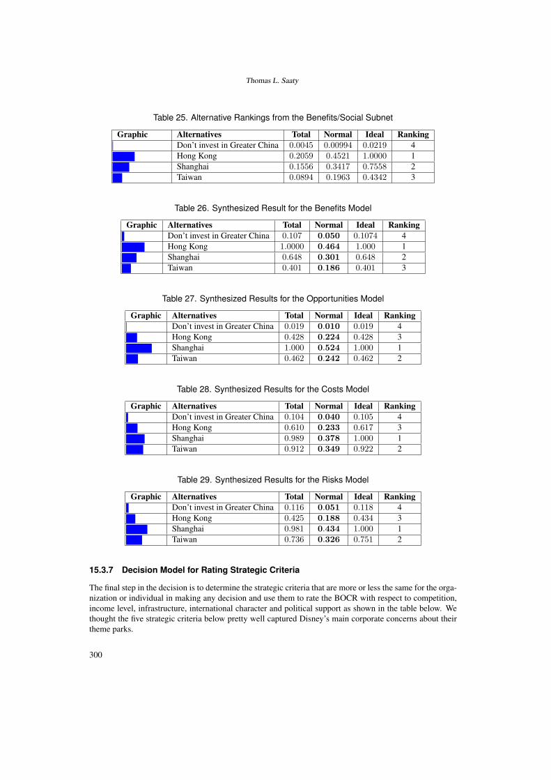
Thomas L. Saaty
Table 25. Alternative Rankings from the Benefits/Social Subnet
Graphic Alternatives Total Normal Ideal RankingDon’t invest in Greater China 0.0045 0.00994 0.0219 4Hong Kong 0.2059 0.4521 1.0000 1Shanghai 0.1556 0.3417 0.7558 2Taiwan 0.0894 0.1963 0.4342 3
Table 26. Synthesized Result for the Benefits Model
Graphic Alternatives Total Normal Ideal RankingDon’t invest in Greater China 0.107 0.050 0.1074 4Hong Kong 1.0000 0.464 1.000 1Shanghai 0.648 0.301 0.648 2Taiwan 0.401 0.186 0.401 3
Table 27. Synthesized Results for the Opportunities Model
Graphic Alternatives Total Normal Ideal RankingDon’t invest in Greater China 0.019 0.010 0.019 4Hong Kong 0.428 0.224 0.428 3Shanghai 1.000 0.524 1.000 1Taiwan 0.462 0.242 0.462 2
Table 28. Synthesized Results for the Costs Model
Graphic Alternatives Total Normal Ideal RankingDon’t invest in Greater China 0.104 0.040 0.105 4Hong Kong 0.610 0.233 0.617 3Shanghai 0.989 0.378 1.000 1Taiwan 0.912 0.349 0.922 2
Table 29. Synthesized Results for the Risks Model
Graphic Alternatives Total Normal Ideal RankingDon’t invest in Greater China 0.116 0.051 0.118 4Hong Kong 0.425 0.188 0.434 3Shanghai 0.981 0.434 1.000 1Taiwan 0.736 0.326 0.751 2
15.3.7 Decision Model for Rating Strategic Criteria
The final step in the decision is to determine the strategic criteria that are more or less the same for the orga-nization or individual in making any decision and use them to rate the BOCR with respect to competition,income level, infrastructure, international character and political support as shown in the table below. Wethought the five strategic criteria below pretty well captured Disney’s main corporate concerns about theirtheme parks.
300
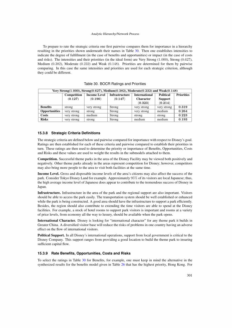
Analytic Hierarchy/Network Process
To prepare to rate the strategic criteria one first pairwise compares them for importance in a hierarchyresulting in the priorities shown underneath their names in Table 30. Then one establishes intensities toindicate the degree of fulfillment (in the case of benefits and opportunities) or impact (in the case of costsand risks). The intensities and their priorities (in the ideal form) are Very Strong (1.000), Strong (0.627),Medium (0.382), Moderate (0.232) and Weak (0.148). Priorities are determined for them by pairwisecomparing. In this case the same intensities and priorities are used for each strategic criterion, althoughthey could be different.
Table 30. BOCR Ratings and Priorities
Very Strong(1.000), Strong(0.627), Medium(0.382), Moderate(0.232) and Weak(0.148)Competition Income Level Infrastructure International Political Priorities
(0.127) (0.190) (0.147) Character Support(0.323) (0.214)
Benefits strong very strong Strong very strong very strong 0.319
Opportunities very strong strong Strong very strong medium 0.264
Costs very strong medium Strong strong strong 0.223
Risks very strong strong Strong medium medium 0.193
15.3.8 Strategic Criteria Definitions
The strategic criteria are defined below and pairwise compared for importance with respect to Disney’s goal.Ratings are then established for each of these criteria and pairwise compared to establish their priorities inturn. These ratings are then used to determine the priority or importance of Benefits, Opportunities, Costsand Risks and these values are used to weight the results in the submodels attached to them.
Competition. Successful theme parks in the area of the Disney Facility may be viewed both positively andnegatively. Other theme parks already in the areas represent competition for Disney; however, competitorsmay also bring more people to the area to visit both facilities at the same time.
Income Level. Gross and disposable income levels of the area’s citizens may also affect the success of thepark. Consider Tokyo Disney Land for example. Approximately 95% of its visitors are local Japanese; thus,the high average income level of Japanese does appear to contribute to the tremendous success of Disney inJapan.
Infrastructure. Infrastructure in the area of the park and the regional support are also important. Visitorsshould be able to access the park easily. The transportation system should be well established or enhancedwhile the park is being constructed. A good area should have the infrastructure to support a park efficiently.Besides, the region should also contribute to extending the time visitors are able to spend at the Disneyfacilities. For example, a stock of hotel rooms to support park visitors is important and rooms at a varietyof price levels, from economy all the way to luxury, should be available when the park opens.
International Character. Disney is looking for “international character” for any theme park it builds inGreater China. A diversified visitor base will reduce the risks of problems in one country having an adverseeffect on the flow of international visitors.
Political Support. In all Disney’s international operations, support from local government is critical to theDisney Company. This support ranges from providing a good location to build the theme park to insuringsufficient capital flow.
15.3.9 Rate Benefits, Opportunities, Costs and Risks
To select the ratings in Table 30 for Benefits, for example, one must keep in mind the alternative in thesynthesized results for the benefits model given in Table 26 that has the highest priority, Hong Kong. For
301

Thomas L. Saaty
example, Hong Kong’s benefits to fulfill the Competition strategic criterion or objective is thought to bestrong. For fulfilling benefits for Income Level, Hong Kong would be very strong as people there have highdisposable income, and so on for all the Strategic Criteria.
When making ratings for Costs and Risks, keep in mind that the highest priority alternative is the mostcostly or most risky. To select the ratings for Risks keep in mind Shanghai. Shanghai has very strong risksso far as Competition is concerned, and strong risks for Income Level as people have less disposable incomethere, and medium risks for Political Support which means the risk is not too great for Disney in Shanghaias they believe they would have the support of the Chinese Government.
The overall priorities for the BOCR are computed by multiplying and adding across each row and nor-malizing the final result shown in the last column of Table 30. The priorities show that the most importantmerit is Benefits at 31.9% followed by Opportunities at 26.4%. This means that the priorities of the alter-natives under benefits are weighted more heavily. Benefits at 31.9% drive the decision more than the Risksat 19.3%.
The final results shown in Table 31 are obtained by using the formula bB + oO − cC − rR where b, o,c and r are the priorities for Benefits, Opportunities, Costs and Risks obtained from rating the strategic cri-teria in Table 30. This formula is applied for the alternatives using the priority vectors from the synthesizedresults (the B, O, C, and R of the formula) in Tables 25–28. Since this formula involves negatives, theoverall synthesized results in Table 30 may be negative, meaning that the alternative is undesirable. Some-times all results are negative, and one is forced to take the least undesirable one. In Table 31 positive resultsare labeled blue and negative red. Here Hong Kong is best with the highest positive value and Taiwan isworst with the highest negative value.
Table 31. BOCR Model: Overall Synthesized Results
Graphic Alternatives Total Normal Ideal Ranking(red) Don’t invest in Greater China −0.006 −0.017 −0.030 3
(blue) Hong Kong 0.214 0.567 1.000 1(blue) Shanghai 0.061 0.161 0.284 2(red) Taiwan −0.096 −0.255 −0.449 4
As we can see, from the overall synthesized results in Table 31, Disney’s best option is to build theirnew theme park in Hong Kong.
15.3.10 Sensitivity Analysis Graphs
In Figures 14, the vertical dotted lines represent the priorities of the BOCR. Starting on the left, the curvesfrom top to bottom are for 1) benefits: Do Nothing, Hong Kong Shanghai, Taiwan, 2) opportunities: HongKong, Do Nothing, Shanghai, Taiwan, 3) and for both costs and risks: Hong Kong, Shanghai, Taiwan, Donothing. Sensitivity analysis in Figure 15 shows that when the importance of benefits is greater than 0.05,investing in Hong Kong is the best choice. The dotted vertical line indicates the priority of Benefits, forexample. To see what happens as the importance of benefits increases, the vertical line can be moved to theright. Above a benefits priority of about 0.39, the least preferred alternative changes from Taiwan to notinvesting in Greater China. The curve immediately under Hong Kong is Shanghai. One might interpret thisas indicating that investing in China somewhere is imperative in terms of benefits.
At an importance of 22.3% for costs, Hong Kong (the top curve) is most costly and Taiwan (the bottomcurve) is least costly, perhaps because of the political uncertainty and lack of supporting infrastructure inHong Kong. As costs increase, not investing in China is the top curve (after about 39%). At an importanceof 19.3% for risks, the top curve is Hong Kong, so it is most risky and the bottom curve is Taiwan, meaningleast risky. When risk is less than about 0.50, the preferred alternative is to invest in Hong Kong. As the
302

Analytic Hierarchy/Network Process
Figure 14. Sensitivity Graphs for the BOCR Networks
importance of risk increases the preferred alternative is to not to invest at all in Greater China, but sincethe priority is negative and lies below the x-axis, this is not a particularly good alternative, though it is theleast negative. Thus, it is extremely risky not to invest in China at all. In sum, the greatest benefits andopportunities lie in mainland China, but also the greatest costs and risks. Netting out both sides, HongKong is the preferred alternative for Disney’s investment.
By way of validation, this study was done before implementation took place. Now, built on lush LantauIsland just 24 minutes from downtown Hong Kong, Disneyland Hong Kong is the fifth Disneyland stylepark in the world offering people a world of adventure and entertainment since its opening in September2005.
16 The Question of Rank Preservation and Reversal in theDiscrete Case
In relative measurement the final priority value associated with each object depends on the values of allthe other objects with which it is compared so that its measurement does not remain constant but dependson what other objects are being measured. Because of this, if objects were to be rank ordered throughcomparisons, their priorities and overall rank order may change when other objects are added or old onesdeleted. In other words rank reversal can occur. It is known that such reversal can never happen when theobjects are compared with respect to one criterion and the judgments are consistent, but only with respectto several criteria. In addition, if it is known that rank must not be allowed to reverse it can be preserved inthe Analytic Hierarchy Process (AHP) using both its “Rating” one at a time approach and its comparisonsapproach. In fact it has been shown experimentally that rank reversal occurs on the average only 8% of thetime, but there is good reason for that [16].
303

Thomas L. Saaty
One consequence of the belief in scales of measurement as the incontestable and unique way of mea-surement is the idea that the measurement of objects can and should be done independently of one anotherand thus the measurement of one object cannot affect the rank order of other objects no matter how im-portant or unimportant the given object may be. It is a natural step to believe that must also be true inmulticriteria decisions where we have measurements of the same objects on not one property but several,using different scales, and wish to combine these measurements using criteria weights or other kinds ofnumbers to develop an overall measurement rank for the alternatives of a decision. This kind of dogmaresults in what has come to be known as rank preservation. At first glance it seems reasonable and com-pelling when an alternative is added or deleted, the criteria weights do not depend on the alternatives andparticularly when no criteria are added or deleted and judgments are changed, a requirement that naturallysuggests itself to suit the process of assigning numbers to objects one at a time.
All decision making methods that rank alternatives one at a time suffer from the following observation.Adding copies or near copies of an alternative until the universe is full of them can depreciate the value andalso the rank of that alternative and, as a counter example, negates the possibility of proving a theorem thatthe rank of independent alternatives must always be preserved when the judgments remain the same and nocriteria are added or deleted or their weights changed. A criterion such as “manyness” that represents thenumber of alternatives cannot be used in the ranking because it forces the dependence of the ranking of eachalternative on the existence of every other alternative thus contradicting the assumption of independence. Itis illogical (or we might say also wrong) for all multicriteria methods that all use the rating of alternativesone at a time not to take this into account.
There have been numerous objections by various authors to the assumption of rank preservation evenwhen things are measured one at a time in the manner described above. In other words, rank is preserved bysome multicriteria methods in cases when, people have argued, it is inappropriate for it to do so and shouldin fact reverse. In other words there are people who have published in the literature who do not believe inthe unconditional rank preservation principle for this kind of measurement.
Three reasons why always preserving rank is not a reliable principle are:
1. There is no theorem or law of nature that confirms the erroneous observation that rank preservationmust always hold in multicriteria measurement when one uses one or several scales of measurementeach of which measures things one at a time. If one does not use such scales, any fact known aboutthe behavior of things that are measured on such scales need not apply. Any convincing example thatviolates rank preservation proves that ranking alternatives one at a time is an inappropriate methodfor multicriteria decision making with independence assumptions all the time.
2. Many papers with examples of rank reversal have been published by distinguished scholars that showlegitimate rank reversals and some authors have gone on to make important statements that forcingrank to be always preserved would produce unreasonable results.
3. Paired comparisons can lead to rank reversal among alternatives when new ones are added or deleted.In fact they show that rank preservation is desirable only when the criteria used to evaluate alternativesare extrinsic outside or top down conditions (not intrinsic attributes) imposed on the alternatives. Inranking the intrinsic attributes one must think of the alternatives, and that is a case of the dependenceof the criteria on the alternatives and when criteria depend on alternatives, anything can happen tothe ranks of the alternatives, that is their ranks can change. But when extrinsic conditions are appliedto the alternatives, their ranks must be preserved. This is also true of intrinsic conditions whoseimportance acquires autonomy over a long time and is not tied to the alternatives one has when adecision is being made.
304

Analytic Hierarchy/Network Process
17 Group Decision MakingHere we consider two issues in group decision making [14]. The first is how to aggregate individual judg-ments into a representative group judgment, and the second is how to construct a group choice from indi-vidual choices. In reality group decisions should not go by consensus because not all people feel the sameabout things. A minority can have very strong commitments to a cause and can give rise to disruptions thatthe majority feels lukewarm about. There is no hiding from this issue in the real world. The reciprocalproperty plays an important role in combining the judgments of several individuals to obtain a judgment fora group. Judgments must be combined so that the reciprocal of the synthesized judgments must be equalto the syntheses of the reciprocals of these judgments. It has been proved that the geometric mean is theunique way to do that. If the individuals are experts, they may not wish to combine their judgments but onlytheir final outcome from a hierarchy. In that case one takes the geometric mean of the final outcomes. If theindividuals themselves have different priorities of importance their judgments (final outcomes) are raised tothe power of their priorities and then the geometric mean is formed. The following is a summary of resultsof research I did with Janos Aczel many years ago [2].
17.1 How to Aggregate Individual Judgments
Let the function f(x1, . . . , xn) for synthesizing the judgments given by n judges, satisfy the
(i) Separability condition (S): f(x1, . . . , xn) = g(x1) · · · g(xn), for all x1, . . . , xn in an interval P ofpositive numbers, where g is a function mapping P onto a proper interval J and is a continuous,associative and cancellative operation. [(S) means that the influences of the individual judgments canbe separated as above.]
(ii) Unanimity condition (U): f(x, . . . , x) = x for all x in P . [(U) means that if all individuals give thesame judgment x, that judgment should also be the synthesized judgment.]
(iii) Homogeneity condition (H): f(ux1, . . . , uxn) = uf(x1, . . . , xn) where u > 0 and xk, uxk (k = 1,2, . . . , n) are all in P . [For ratio judgments (H) means that if all individuals judge a ratio u times aslarge as another ratio, then the synthesized judgment should also be u times as large.]
(iv) Power conditions (Pp): f(xp1, . . . , x
pn) = fp(x1, . . . , xn). [(P2) for example means that if the kth
individual judges the length of a side of a square to be xk, the synthesized judgment on the area ofthat square will be given by the square of the synthesized judgment on the length of its side.] Specialcase (R = P−1):
f
(1x1
, . . . ,1xn
)=
1f(x1, . . . , xn)
.
[(R) is of particular importance in ratio judgments. It means that the synthesized value of the recip-rocal of the individual judgments should be the reciprocal of the synthesized value of the originaljudgments.] Aczel and Saaty [13] proved the following theorem:
Theorem 2. The general separable (S) synthesizing functions satisfying the unanimity (U) and homogene-
ity (H) conditions are the geometric mean and the root-mean-power. If moreover the reciprocal property
(R) is assumed even for a single n-tuple of the judgments of n individuals, where not all xk are equal, then
only the geometric mean satisfies all the above conditions.
In any rational consensus, those who know more should, accordingly, influence the consensus morestrongly than those who are less knowledgeable. Some people are clearly wiser and more sensible in suchmatters than others, others may be more powerful and their opinions should be given appropriately greaterweight. For such unequal importance of voters not all g’s in (S) are the same function. In place of (S), theweighted separability property (WS) is now: f(x1, . . . , xn) = g1(x1) · · · gn(xn) [(WS) implies that not all
305

Thomas L. Saaty
judging individuals have the same weight when the judgments are synthesized and the different influencesare reflected in the different functions (g1, . . . , gn).]
In this situation, Aczel and Alsina [1] proved the following theorem:
Theorem 3. The general weighted-separable (WS) synthesizing functions with the unanimity (U) and
homogeneity (H) properties are the weighted geometric mean f(x1, x2, . . . , xn) = xq11 xq2
2 · · ·xqnn and the
weighted root-mean- powers f(x1, x2, . . . , xn) = γ√
q1xγ1 + q2x
γ2 + · · ·+ qnxγ
n, where q1+q2+· · ·+qn =1, qk > 0, k = 1, 2, . . . , n, γ > 0, but otherwise q1, q2, . . . , qn, γ are arbitrary constants.
If f also has the reciprocal property (R) and for a single set of entries (x1, . . . , xn) of judgments of nindividuals, where not all xk are equal, then only the weighted geometric mean applies.
We give the following theorem which is an explicit statement of the synthesis problem that follows fromthe previous results:
Theorem 4. If x(i)1 , x
(i)2 , . . . , x
(i)n , i = 1, . . . , m are rankings of n alternatives by m independent
judges and if ai is the importance of judge i developed from a hierarchy for evaluating the judges, and
hence∑m
i=1 ai = 1, then (∏m
i=1 xai1 ), . . . , (
∏mi=1 xai
n ) are the combined ranks of the alternatives for the mjudges.
Note that essentially the geometric mean raises each judgment to the default power of 1/n as if eachindividual’s judgment is as important as any other individual. The power or priority of judge i is simply areplication of the judgment of that judge (as if there are as many other judges as indicated by his/her powerai), which implies multiplying his/her ratio by itself ai times, and the result follows.
The following useful theorem was proved in a joint, yet to be published work, with my friend andcolleague Luis G. Vargas. It shows how important it is to debate issues in order to mitigate extreme positionsas much as we can to make it easier for groups to agree and act cooperatively on their decisions.
Theorem 5 (Bounded Inconsistency). For a group of inconsistent individuals, the inconsistency of
group judgments aggregated by the geometric mean from individual judgments is at most equal to the
largest of the individual inconsistencies.
PROOF. First we show that the inconsistency of a group along cycles of length three satisfies thistheorem and is related to the inconsistency index given by
μk ≡ λ(k)max − n
n− 1= −1 +
1n(n− 1)
∑1≤i<j≤n
(εijk +
1εijk
)
where λ(k)max is the principal eigenvalue of the matrix (aijk = wik
wjkεijk) . Thus, we have λ
(k)maxwik =∑
j aijkwjk =∑
jwik
wjkεijkwjk = wik
∑j εijk and λ
(k)max =
∑j εijk for all i.
Let (aijk = wik
wjkεijk), k = 1, 2, . . . , m be the n-by-n matrices of pairwise comparisons of m indi-
viduals. Let δijk = εijk − 1. By definition inconsistency in the judgments of an individual means thataijkajlk �= ailk for at least some i, j and l. The inconsistency of a 3-cycle for the kth individual can bemeasured by aijkajlkalik. Clearly, if these judgments were consistent aijkajlkalik = 1 for all i, j and l.Thus, inconsistency can be measured with an index that must exclude loops that only connect judgmentswith themselves preventing the formation of 3-cycles. We have
Ik(n, 3) =1
n(n− 1)(n− 2)
∑i �=j �=l
aijkajlkalik =1
n(n− 1)(n− 2)
∑i �=j �=l
εijkεjlkεlik
306
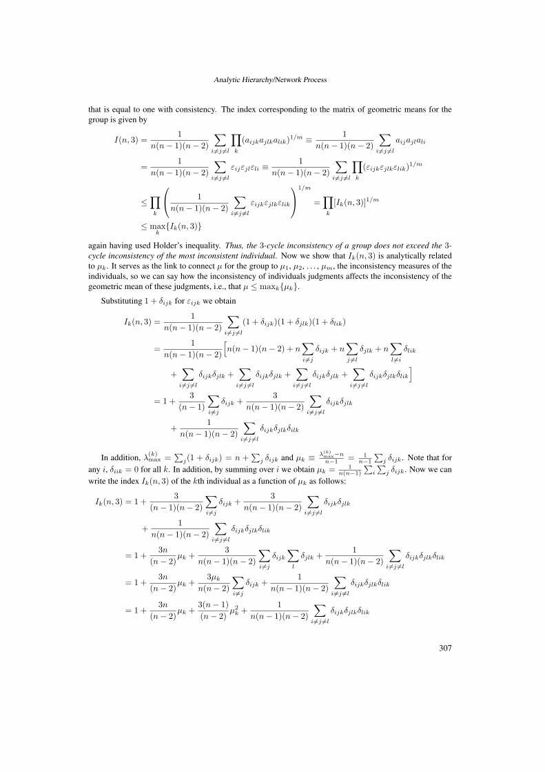
Analytic Hierarchy/Network Process
that is equal to one with consistency. The index corresponding to the matrix of geometric means for thegroup is given by
I(n, 3) =1
n(n− 1)(n− 2)
∑i �=j �=l
∏k
(aijkajlkalik)1/m ≡ 1n(n− 1)(n− 2)
∑i �=j �=l
aijajlali
=1
n(n− 1)(n− 2)
∑i �=j �=l
εijεjlεli ≡ 1n(n− 1)(n− 2)
∑i �=j �=l
∏k
(εijkεjlkεlik)1/m
≤∏k
⎛⎝ 1
n(n− 1)(n− 2)
∑i �=j �=l
εijkεjlkεlik
⎞⎠
1/m
=∏k
[Ik(n, 3)]1/m
≤ maxk{Ik(n, 3)}
again having used Holder’s inequality. Thus, the 3-cycle inconsistency of a group does not exceed the 3-
cycle inconsistency of the most inconsistent individual. Now we show that Ik(n, 3) is analytically relatedto μk. It serves as the link to connect μ for the group to μ1, μ2, . . . , μm, the inconsistency measures of theindividuals, so we can say how the inconsistency of individuals judgments affects the inconsistency of thegeometric mean of these judgments, i.e., that μ ≤ maxk{μk}.
Substituting 1 + δijk for εijk we obtain
Ik(n, 3) =1
n(n− 1)(n− 2)
∑i �=j �=l
(1 + δijk)(1 + δjlk)(1 + δlik)
=1
n(n− 1)(n− 2)
[n(n− 1)(n− 2) + n
∑i �=j
δijk + n∑j �=l
δjlk + n∑l �=i
δlik
+∑
i �=j �=l
δijkδjlk +∑
i �=j �=l
δijkδjlk +∑
i �=j �=l
δijkδjlk +∑
i �=j �=l
δijkδjlkδlik
]
= 1 +3
(n− 1)
∑i �=j
δijk +3
n(n− 1)(n− 2)
∑i �=j �=l
δijkδjlk
+1
n(n− 1)(n− 2)
∑i �=j �=l
δijkδjlkδilk
In addition, λ(k)max =
∑j(1 + δijk) = n +
∑j δijk and μk ≡ λ(k)
max−nn−1 = 1
n−1
∑j δijk. Note that for
any i, δiik = 0 for all k. In addition, by summing over i we obtain μk = 1n(n−1)
∑i
∑j δijk. Now we can
write the index Ik(n, 3) of the kth individual as a function of μk as follows:
Ik(n, 3) = 1 +3
(n− 1)(n− 2)
∑i �=j
δijk +3
n(n− 1)(n− 2)
∑i �=j �=l
δijkδjlk
+1
n(n− 1)(n− 2)
∑i �=j �=l
δijkδjlkδlik
= 1 +3n
(n− 2)μk +
3n(n− 1)(n− 2)
∑i �=j
δijk
∑l
δjlk +1
n(n− 1)(n− 2)
∑i �=j �=l
δijkδjlkδlik
= 1 +3n
(n− 2)μk +
3μk
n(n− 2)
∑i �=j
δijk +1
n(n− 1)(n− 2)
∑i �=j �=l
δijkδjlkδlik
= 1 +3n
(n− 2)μk +
3(n− 1)(n− 2)
μ2k +
1n(n− 1)(n− 2)
∑i �=j �=l
δijkδjlkδlik
307

Thomas L. Saaty
In a neighbohood of εij = 1 corresponding to near consistency we have
Ik(n, 3) = 1 +3n
(n− 2)μk + o(δijk)
and for the group index I(n, 3) by simply suppressing the subscript k above:
I(n, 3) = 1 +3
(n− 1)(n− 2)
∑i �=j
δij +3
n(n− 1)(n− 2)
∑i �=j �=l
δijδjl +1
n(n− 1)(n− 2)
∑i �=j �=l
δijδjlδli
= 1 +3n
(n− 2)μ + o(δij)
Thus, finaly I(n, 3) = 1+3n
n− 2μ+o(δij) ≤ maxk
{1 +
3n
n− 2μk + o(δijk)
}and μ ≤ maxk{μk}. �
17.2 On the Construction of Group Choice from Individual ChoicesGiven a group of individuals, a set of alternatives (with cardinality greater than 2), and individual ordinalpreferences for the alternatives, Kenneth Arrow [3] who won the Nobel Prize for his work on this theoremproved with his Impossibility Theorem that it is impossible to derive a rational group choice (construct asocial choice function that aggregates individual preferences) from ordinal preferences of the individualsthat satisfy the following four conditions, i.e., at least one of them is violated:
• Decisiveness: the aggregation procedure must generally produce a group order.
• Unanimity: if all individuals prefer alternative A to alternative B, then the aggregation proceduremust produce a group order indicating that the group prefers A to B.
• Independence of irrelevant alternatives: given two sets of alternatives which both include A and B, ifall individuals prefer A to B in both sets, then the aggregation procedure must produce a group orderindicating that the group, given any of the two sets of alternatives, prefers A to B.
• No dictator: no single individual preferences determine the group order.
Using Fundamental Scale of absolute numbers of the AHP, it can be shown that because now the indi-vidual preferences are cardinal rather than ordinal, it is possible to derive a rational group choice satisfyingthe above four conditions. We proved this with L. G. Vargas [18]. It is possible because: a) Individualpriority scales can always be derived from a set of pairwise cardinal preference judgments as long as theyform at least a minimal spanning tree in the completely connected graph of the elements being compared;and b) The cardinal preference judgments associated with group choice belong to an absolute scale thatrepresents the relative intensity of the group preferences.
18 Generalization to the Continuous CaseThe foregoing discrete formulation with
n∑j=1
aijwj = λmaxwi (1)
n∑i=1
wi = 1 (2)
308
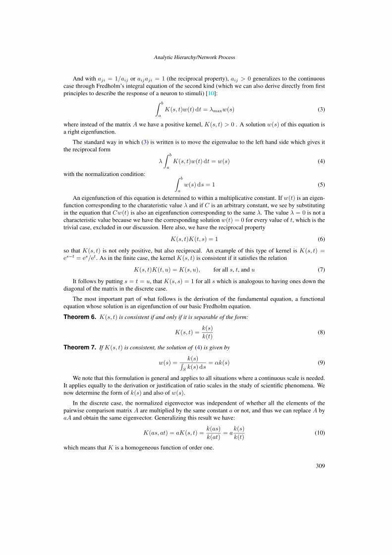
Analytic Hierarchy/Network Process
And with aji = 1/aij or aijaji = 1 (the reciprocal property), aij > 0 generalizes to the continuouscase through Fredholm’s integral equation of the second kind (which we can also derive directly from firstprinciples to describe the response of a neuron to stimuli) [10]:∫ b
a
K(s, t)w(t) dt = λmaxw(s) (3)
where instead of the matrix A we have a positive kernel, K(s, t) > 0 . A solution w(s) of this equation isa right eigenfunction.
The standard way in which (3) is written is to move the eigenvalue to the left hand side which gives itthe reciprocal form
λ
∫ b
a
K(s, t)w(t) dt = w(s) (4)
with the normalization condition: ∫ b
a
w(s) ds = 1 (5)
An eigenfunction of this equation is determined to within a multiplicative constant. If w(t) is an eigen-function corresponding to the charateristic value λ and if C is an arbitrary constant, we see by substitutingin the equation that Cw(t) is also an eigenfunction corresponding to the same λ. The value λ = 0 is not acharacteristic value because we have the corresponding solution w(t) = 0 for every value of t, which is thetrivial case, excluded in our discussion. Here also, we have the reciprocal property
K(s, t)K(t, s) = 1 (6)
so that K(s, t) is not only positive, but also reciprocal. An example of this type of kernel is K(s, t) =es−t = es/et. As in the finite case, the kernel K(s, t) is consistent if it satisfies the relation
K(s, t)K(t, u) = K(s, u), for all s, t, and u (7)
It follows by putting s = t = u, that K(s, s) = 1 for all s which is analogous to having ones down thediagonal of the matrix in the discrete case.
The most important part of what follows is the derivation of the fundamental equation, a functionalequation whose solution is an eigenfunction of our basic Fredholm equation.
Theorem 6. K(s, t) is consistent if and only if it is separable of the form:
K(s, t) =k(s)k(t)
(8)
Theorem 7. If K(s, t) is consistent, the solution of (4) is given by
w(s) =k(s)∫
Sk(s) ds
= αk(s) (9)
We note that this formulation is general and applies to all situations where a continuous scale is needed.It applies equally to the derivation or justification of ratio scales in the study of scientific phenomena. Wenow determine the form of k(s) and also of w(s).
In the discrete case, the normalized eigenvector was independent of whether all the elements of thepairwise comparison matrix A are multiplied by the same constant a or not, and thus we can replace A byaA and obtain the same eigenvector. Generalizing this result we have:
K(as, at) = aK(s, t) =k(as)k(at)
= ak(s)k(t)
(10)
which means that K is a homogeneous function of order one.
309

Thomas L. Saaty
Theorem 8. A necessary and sufficient condition for w(s) to be an eigenfunction solution of Fredholm’s
equation of the second kind, with a consistent kernel that is homogeneous of order one is that it satisfy the
functional equation
w(as) = bw(s) (11)
where b = αa.
It is clear that whatever aspect of the real world we consider, sight, sound, touch, taste, smell, heatand cold, at each instant, their corresponding stimuli impact our senses numerous times. A stimulus Sof magnitude s, is received as a similarity transformation as, a > 0 referred to as a dilation of s. It is astretching if a > 1, and a contraction if a < 1. When relating response to a dilated stimulus of magnitudeas to response to an unaltered stimulus whose magnitude is s, we have the proportionality relation betweenresponding to an altered stimulus and to the original stimulus given in (11) as
w(as)w(s)
= b
We refer to equation (11) as: The Functional Equation of Ratio Scales. Because of its wider implica-tions in science, we may call it: The Fundamental Equation of Proportionality and Order [10]. We couldhave written down this equation directly from what we know about responding to stimuli with the ideaof exercising control for which there also has to be proportionality. This would be true for a compositestimulus consisting of many stimuli thus defining s function instead of a single variable.
If we substitute s = au in (11) we have w(au+1)− bw(au) = 0 (I am grateful to my friend Janos Aczelthe world leader in functional equations for his help in deriving (12) and (13) below):
Again if we write,w(au) = bup(u)
we get:p(u + 1)− p(u) = 0
which is a periodic function of period one in the variable u (such as cos u/2π). Note that if a and s are real,then so is u which may be negative even if a and s are both assumed to be positive.
If in the last equation p(0) is not equal to 0, we can introduce C = p(0) and P (u) = p(u)/C, we havefor the general response function w(s):
w(s) = Celog b log slog a P
(log s
log a
)(12)
where P is also periodic of period 1 and P (0) = 1. Note that C > 0 only if p(0) is positive. Otherwise, ifp(0) < 0, C < 0.
Near zero, the exponential factor, which is equal to slog b/ log a , “slims” w(s) if log b/ log a > 0 and“spreads” w(s) if log b/ log a < 0. Because s is the magnitude of a stimulus and cannot be negative, wedo not have a problem with complex variables here so long as both a and b are real and both positive. Oursolution in the complex domain has the form:
w(z) = zln b/ ln aP
(ln z
ln a
)(13)
Here P (u) with u = ln z/ ln a, is an arbitrary multivalued periodic function in u of period 1. Evenwithout the multivaluedness of P , the function w(z) could be multivalued because ln b/ ln a is generally acomplex number. If P is single-valued and ln b/ ln a turns out to be an integer or a rational number, thenw(z) is a single-valued or finitely multivalued function, respectively. This generally multivalued solution isobtained in a way analogous to the real case.
310

Analytic Hierarchy/Network Process
This Solution Leads to the Weber-Fechner LawNote in (12) that the periodic function P (u) is bounded and the negative exponential leads to an alternatingseries. Thus, to a first order approximation in series expansion, one obtains the Weber-Fechner law a log s+b for response to a stimulus s. We assume that b = 0, and hence the response belongs to a ratio scale. Recallthat in making comparisons, we form the ratio of two ratio scale readings which is a dimensionless numberand belongs to the Fundamental Scale of absolute numbers.
Stimuli received by the brain from nature are transformed to chemical and electrical neural activities thatresult in summation and synthesis. This is transformed to awareness of nature by converting the electricalsynthesis (vibrations caused by a pattern) to a space-time representation. The way the brain goes back andforth from a pattern of stimuli to its electro-chemical synthesis and then to a representation of its responseto that spacio-temporal pattern is by applying the Fourier transform to the stimulus and the inverse Fouriertransform to form its response. What we have been doing so far is concerned with the inverse Fouriertransform. We now need to take its inverse to develop expressions for the response.
We now show that the space-time Fourier transform of (13) is a combination of Dirac distributions. Oursolution of Fredholm’s equation here is given as the Fourier transform,
f(ω) =∫ +∞
∞F (x)e−2πiωx dx = CeβωP (w) (14)
whose inverse transform is given by:
12π
log a∞∑−∞
a′n
[(2πn + θ(b)− x)
(log a|b|+ (2πn + θ(b)− x))i
]δ(2πn + θ(b)− x) (15)
where δ(2πn + θ(b) − x) is the Dirac delta function which means that the way we respond to stimuli hasthe form of the delta firings as indeed it is known that our neurons behave. Neural responses are impulsiveand hence the brain is a discrete firing system. This is supporting evidence in favor of the generalizedcomparisons model.
19 The Formation of Images and Sounds with Dirac Distribu-tions
Complex valued functions with their imaginary part cannot be drawn as one does ordinary functions ofthree real variables. Nevertheless, one can make a plot of the modulus or absolute value of such a function.The basic assumption we made to represent the response to a sequence of individual stimuli is that all thelayers in a network of neurons are identical, and each stimulus value is represented by the firing of a neuronin each layer. A shortcoming of this representation is that it is not invariant with respect to the order inwhich the stimuli are fed into the network. It is known in the case of vision that the eyes do not scanpictures symmetrically if they are not symmetric, and hence our representation must satisfy some orderinvariant principle. Taking into account this principle would allow us to represent images independentlyof the form in which stimuli are input into the network. For example, we recognize an image even if it issubjected to a rotation, or to some sort of deformation. Thus, the invariance principle must include affineand similarity transformations. This invariance would allow the network to recognize images even whenthey are not identical to the ones from which it recorded a given concept, e.g., a bird. The next step wouldbe to use the network representation given here with additional conditions to uniquely represent patternsfrom images, sounds and perhaps other sources of stimuli such as smell. Our representation focuses on thereal part of the magnitude rather than the phase of the Fourier transform. Tests have been made to see theeffect of phase and of magnitude on the outcome of a representation of a complex valued function. Thereis much more blurring due to change in magnitude than there is to change in phase. Thus we focus on
311

Thomas L. Saaty
representing responses in terms of Dirac functions, sums of such functions, and on approximations to themwithout regard to the coefficients in (15).
Because finite linear combinations of the functions {tαe−βt, α, β ≥ 0} are dense in the space ofbounded continuous functions C[0, b] we used them to represent images and sounds [17].
We created a 2-dimensional network of neurons consisting of layers. For illustrative purposes, weassumed that there is one layer of neurons corresponding to each of the stimulus values. Thus, if the list ofstimuli consists of n numerical values, we created n layers with a specific number of neurons in each layer.Under the assumption that each numerical stimulus is represented by the firing of one and only one neuron,each layer of the network must also consist of n neurons with thresholds varying between the largest andthe smallest values of the list of stimuli. We also assumed that the firing threshold of each neuron had thesame width. Thus, if the perceptual range of a stimulus varies between two values θ1 and θ2, and each layerof the network has n neurons, then a neuron in the ith position of the layer will fire if the stimulus valuefalls between
θ1 + (i− 1)θ2 − θ1
n− 1and θ1 + i
θ2 − θ1
n− 1
19.1 Picture Experiment
In the graphics experiment the bird and rose pictures required 124 and 248 data points, respectively, whereasthe sound experiment required 1000 times more data points. Once the (x, y) coordinates of the pointswere obtained, the x-coordinate was used to represent time and the y-coordinate to represent response to astimulus. The numerical values associated with the drawings in Figures 15 and 16 were tabulated and thenumbers provided the input to the neurons in the networks built to represent the bird and the rose.
Figure 15. Bird
Figure 16. Rose
312
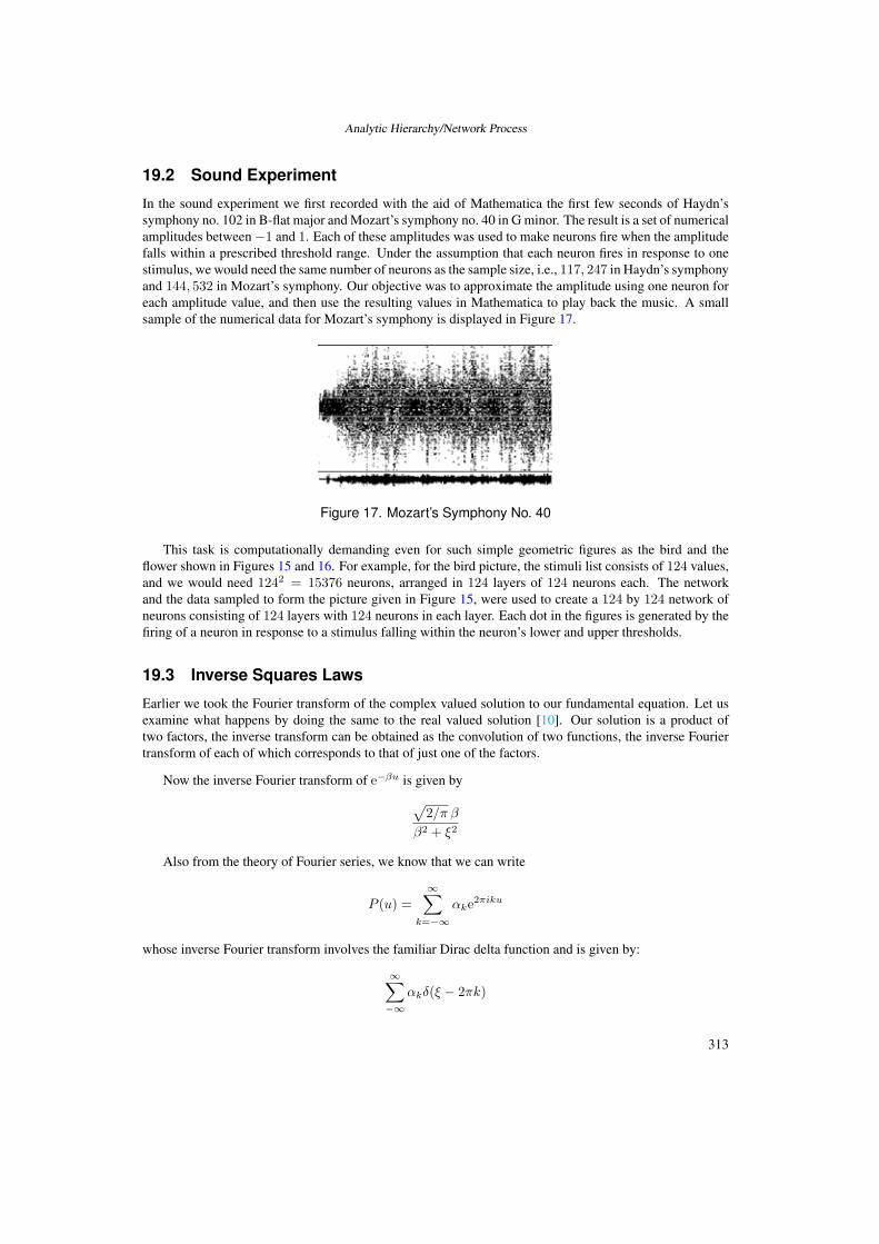
Analytic Hierarchy/Network Process
19.2 Sound Experiment
In the sound experiment we first recorded with the aid of Mathematica the first few seconds of Haydn’ssymphony no. 102 in B-flat major and Mozart’s symphony no. 40 in G minor. The result is a set of numericalamplitudes between−1 and 1. Each of these amplitudes was used to make neurons fire when the amplitudefalls within a prescribed threshold range. Under the assumption that each neuron fires in response to onestimulus, we would need the same number of neurons as the sample size, i.e., 117, 247 in Haydn’s symphonyand 144, 532 in Mozart’s symphony. Our objective was to approximate the amplitude using one neuron foreach amplitude value, and then use the resulting values in Mathematica to play back the music. A smallsample of the numerical data for Mozart’s symphony is displayed in Figure 17.
Figure 17. Mozart’s Symphony No. 40
This task is computationally demanding even for such simple geometric figures as the bird and theflower shown in Figures 15 and 16. For example, for the bird picture, the stimuli list consists of 124 values,and we would need 1242 = 15376 neurons, arranged in 124 layers of 124 neurons each. The networkand the data sampled to form the picture given in Figure 15, were used to create a 124 by 124 network ofneurons consisting of 124 layers with 124 neurons in each layer. Each dot in the figures is generated by thefiring of a neuron in response to a stimulus falling within the neuron’s lower and upper thresholds.
19.3 Inverse Squares Laws
Earlier we took the Fourier transform of the complex valued solution to our fundamental equation. Let usexamine what happens by doing the same to the real valued solution [10]. Our solution is a product oftwo factors, the inverse transform can be obtained as the convolution of two functions, the inverse Fouriertransform of each of which corresponds to that of just one of the factors.
Now the inverse Fourier transform of e−βu is given by
√2/π β
β2 + ξ2
Also from the theory of Fourier series, we know that we can write
P (u) =∞∑
k=−∞αke2πiku
whose inverse Fourier transform involves the familiar Dirac delta function and is given by:
∞∑−∞
αkδ(ξ − 2πk)
313

Thomas L. Saaty
The product of the transforms of the two functions is equal to the Fourier transform of the convolutionof the two functions themselves that we just obtained by taking their individual inverse transforms. Wehave, to within a multiplicative constant:
∫ ∞
−∞
∞∑k=−∞
αkδ(ξ − 2πk)β
β2 + (x− ξ)2dξ =
∞∑k=−∞
αkβ
β2 + (x− 2πk)2
The inverse Fourier transform of w(u) = Ce−βu cos u2π , β > 0 is given by:
C
[1
β2 + (x + 2π)2+
1β2 + (x− 2π)2
]
When the constants in the denominator are small relative to x we have C1/x2 which we believe is whyin optics, gravitation (Newton) and electricity (Coulomb) our response to the forces is according to inversesquare laws. This is the same law of nature in which an object responding to a force field must decideto follow that law by comparing infinitesimal successive states through which it passes. If the stimulusis constant, the exponential factor in the general response solution is constant, and the solution would beperiodic of period one. When the distance x is very small, the result varies inversely with the parameterβ > 0. It appears that the inverse square law is not strictly an inverse square and its use may sometimeslead to difficulty as found with the orbit of Mercury.
20 Generalization to Multiple StimuliWith multiple stimuli we have the functional equation
w(a1z1, . . . , anzn) = bw(z1, . . . , zn)
whose solution for the real variable case with b > 0, ak > 0, and sk > 0, is
w(s1, . . . , sn) = bPn
k=1(log sk/ log ak)/k P
(log s1
log a1, . . . ,
log sn
log an
), k = 1, . . . , n,
where P is an arbitrary periodic function of period one of n variables, that is,
P (u1 + 1, . . . , un + 1) = P (u1, . . . , un)
Solution of the functional equation in the complex domain was communicated to me by my friend themathematician Karol Baron of Katowice, Poland.
w(z1, . . . , zN ) = zk11 · · · zkN
N G
(|z1|, . . . , |zM |, log|zM+1|
log|aM+1| , . . . ,log|zN |log|aN | , arg z1, . . . , arg zN
)
where G is a doubly periodic function with periods
(0, . . . , 0M
, 1, . . . , 1M−N
, arg a1, . . . , arg aN ) and (0, . . . , 0, 2π, 0, . . . , 0(n+l)
)
for l ∈ {1, . . . , N}. It is known that a single-valued analytic function cannot possess more than two linearlyindependent periods.
For a continuum number of stimuli let K(X,Y) be a compact reciprocal kernel i.e. K(x, y)K(y, x) =1, for all x ∈ X and y ∈ Y, where X and Y are compact subsets of the reals. We have the equationw(X = λ
∫Ω
K(X;Y)w(Y) dY for which by analogy with the necessary condition for the solvability
314

Analytic Hierarchy/Network Process
of Fredholm’s equation (4) and ensuing discussion, the following operator functional equation must besatisfied in order for the above equation to have a solution: w[af(x)] = b[f(x)]. This operator linear func-tional equation has been formally and completely solved at Nantes France by Nicole Brillouet-Belluot [5].Because of space limitations here, its solution and interpretation will be described in some detail in myforthcoming book concerned with the generalization of pairwise comparisons to the continuous case.
21 Criticisms of the AHPEssentially, there have been five types of criticisms of the AHP all of which have been addressed in theliterature [19]. One, already mentioned in the paper, is the concern with illegitimate changes in the ranks ofthe alternatives, called rank reversal, upon changing the structure of the decision. It was believed that rankreversal is legitimate only when criteria or priorities of criteria or changes in judgments are made. Rankreversals were shown by critics to occur when using comparisons and relative measurement that is essential
in prioritizing criteria and also alternatives on intangible criteria in two ways: First, when new alternativesare added or old ones deleted; and second, when new criteria are added or old ones deleted with the caveatthat the priorities of the alternatives would be tied under these criteria and hence argued that the criteriashould be irrelevant when ranking the alternatives. Rank reversals that followed such structural changeswere attributed to the use of relative measurement and normalization. Rating alternatives one at a timewith respect to the criteria using the ideal mode, always preserves rank. Also, the ideal mode is used withpaired comparisons to preserve rank. But rank can and should reverse under more general conditions thanhad previously been recognized as in introducing copies or near copies of alternatives and criteria turn outnot to always be so strictly independent among themselves and from the alternatives. The second concernis about inconsistent judgments and their effect on aggregating such judgments or on deriving prioritiesfrom them. A modicum of intransitivity and numerical inconsistency, usually not considered or thoughtto be permissible in other theories, is permissible in the AHP so that decisions can be treated realisticallyrather than axiomatically truncated. A condition that may not hold with inconsistent judgments is Paretooptimality. Pareto optimality is an ordinal relation which demands of a method used to aggregate judgmentsof individuals in a group to a representative collective judgment for that group that when all individuals inthe group prefer A to B then the group judgment must prefer A to B. Because in the AHP judgmentsare not ordinal, it is possible to aggregate the individual judgments into a representative group judgmentwith or without Pareto optimality. Another condition also inherited from expected utility theory has todo with a relation called Condition of Order Preservation (COP): For all alternatives x1, x2, x3, x4, suchthat x1 dominates x2 and x3 dominates x4, if the evaluator’s judgments indicate the extent to which x1
dominates x2 is greater than the extent to which x3 dominates x4, then the vector of priorities w shouldbe such that, not only w(x1) > w(x2) and w(x3) > w(x4) (preservation of order of preference) butalso that w(x1)
w(x2)> w(x3)
w(x4)(preservation of order of intensity of preference). This condition holds when
judgments are consistent but may or may not hold when they are inconsistent. It is axiomatically imposed,sacrificing the original intent of the AHP process to derive priorities that match the reality represented bythe judgments without forcing consistency. The third criticism has to do with attempts to preserve rank fromirrelevant alternatives by combining the comparison judgments of a single individual using the geometricmean (logarithmic least squares) to derive priorities and also combining the derived priorities on differentcriteria by using multiplicative weighting synthesis. The fourth criticism has to do with people trying tochange the fundamental scale despite the fact that it is theoretically derived and tested by comparing it withnumerous other scales on a multiplicity of examples for which the answer was known. The fifth and finalcriticism has to do with whether or not the pairwise comparisons axioms are behavioral and spontaneous innature to provide judgments.
Interestingly, the AHP/ANP provides a way to make complex decisions in the most general structuresencountered in real life. It makes it possible to derive priorities for all the factors in such structures andsynthesize them for an overall outcome, as no other method can because one can build scales for tangiblesand intangibles, yet we know little about criticisms of framing and validating problems within such a wide
315

Thomas L. Saaty
perspective that includes structures, not only for dependence and feedback, but also for benefits, opportuni-ties, costs and risks analyzed separately and then synthesized for the final outcome or in conflict resolutionwith or without a moderating negotiator
22 Conclusions
The AHP/ANP is a useful way to deal with complex decisions that involve dependence and feedback an-alyzed in the context of benefits, opportunities, costs and risks. It has been applied literally to hundredsof examples both real and hypothetical. What is important in decision making is to produce answers thatare valid in practice. The AHP/ANP has also been validated in many examples. People often argue thatjudgment is subjective and that one should not expect the outcome to correspond to objective data. Butthat puts one in the framework of garbage in garbage out without the assurance of the long term validity ofthe outcome. In addition, most other approaches to decision making are normative. They say, “If you arerational you do as I say.” But what people imagine is best to do and what conditions their decisions faceafter they are made can be very far apart from what can happen in the real world. That is why the frameworkof the AHP/ANP is descriptive as in science rather than normative and prescriptive giving license to unreal-istic assumptions like insisting on transitivity of preferences when we know that people are intransitive andinconsistent. The AHP/ANP produce outcomes that are best not simply according to the decision maker’svalues, but also to the external risks and hazards faced by the decision.
It is unfortunate that there are people who use fuzzy sets without proof to alter the AHP when it is knownthat fuzzy applications to decision making have been ranked as the worst among all methods. Because ofthe Weber-Fechner observation, the fundamental scale used in the AHP/ANP to represent judgments isalready fuzzy. To fuzzify it further does not improve the outcome as we have shown through numerousexamples [15]. The intention of fuzzy seems to be to perturb the judgments in the AHP. It is already knownin mathematics that perturbing the entries of a matrix perturbs the eigenvector by a small amount but notnecessarily in a more valid direction.
The SuperDecisions software used to analyze complex decisions is named after the supermatrix. Itcan be downloaded free from creativedecisions.net and is available on the internet along with a manualand with numerous applications to enable the reader to apply it to his/her decision. Alternatively, go towww.superdecisions.com/ saaty and download the SuperDecisions software. The installation file is the.exe file in the software folder. The serial number is located in the .doc file that is in the same folder.The important thing may be not the software but the models which are in a separate folder called models.The military are constantly involved in making complex decisions and appear to like using the ANP andinvesting in its development. Why do we do all this with so much effort? Because we believe strongly inthe creativity of the human race and hope that our world will become increasingly more rational in makingits decisions and in resolving its conflicts.
Since 1976, a very large number of case studies using the Analytic Hierarchy Process in conflict reso-lution, on which I co-authored a book, have been developed. The hope in this work was that, by teachingpeople to analyze their conflicts and to lay bare the structure, reason would prevail and antagonist would bemotivated to come to a reasonable and just solution.
But, in a conflict, particularly one of long duration, reason rarely prevails. Instead, positions becomeentrenched and people seek not only to satisfy their own needs but also to punish their opponents for havingopposed them -or, at least, to pay a price for their opposition.
New light may often be shed on a conflict. Experience has shown that a conflict may be alleviated by theuse of a mediator who introduces “bargaining chips” into the negotiations. If A and B are the participants,A will look at this particular item and evaluate not only the incremental benefits to be received but also thecost to the opponent of providing the concession: The greater each value, the greater the gain.
316

Analytic Hierarchy/Network Process
Thus A’s gain for a given item may be described as the product of A’s benefits and B’s cost (as Aperceives them). We have the following ratios for the two parties A and B:
(as perceived by A)
A’s ratiogain to A
A’s perception of gain to B=∑
A’s benefits×B’s costs∑B’s benefits×A’s costs
=gain to A
loss to A
where∑
is the sum taken over all concessions by B in the numerator and by A in the denominator. A’sperceived ratio for B is the reciprocal of the above:
(as perceived by B)
B’s ratiogain to B
B’s perception of gain to A=∑
B’s benefits×A’s costs∑A’s benefits×B’s costs
=gain to B
loss to B
If both A and B perceive costs and benefits in the same way, these ratios would be reciprocal of eachother. This almost never happens, however.
Obviously, each party would like its ratio to be as high as possible, If A’s ratio for some package is lessthan 1, then A will perceive B’s ratio as being greater than 1 and will feel that it has not been treated fairly.The aim must be to find single concessions and groups of concessions where each party perceive its ownratio to be greater than 1. This requires skilled mediation.
It is wise to involve the parties and to gain their trust so that the necessary estimates may be made. Ifthis is not possible, then the analyst must use his or her best judgements for these.
The ideas were applied to the conflict in South Africa in 1986 in a study paid for at the time by thegovernment of South Africa and whose conclusions appear to have been followed fairly accurately. It issummarized as Chapter 11 of my book on Conflict Resolution. In addition to applying the process to analyzethe conflict in Northern Ireland by my colleague Joyce Alexander since the 1970’s, I have been involvedin work and publication of material that deals with the conflict between Israel and the Palestinians in theMiddle East with the participation of distinguished individuals from that part of the world. What one learnsis that the AHP/ANP provides an opportunity to map out and quantify all the factors in a conflict as desiredby the parties and subject them to sensitivity analysis in the hope of finding an acceptable solution withoutresort to uncivilized behaviour and to violence. One derives a salutary degree of satisfaction from doingthis kind of mathematics that may help save the lives of many people and move us into a new era of usefulnegotiation before commitment to take violent action.
Acknowledgement. My thanks go to Luis Vargas, Rozann Whitaker, Orrin Cooper and José ManuelMagallanes for their editorial help in preparing the manuscript.
References[1] ACZEL, J. AND ALSINA, C., (1986). On synthesis of judgments, Socio-Economic Planning Sciences, 20, 333–
339.
[2] ACZEL, J. AND SAATY, T. L., (1983). Procedures for synthesising ratio judgments, Journal of Mathematical
Psychology, 27, 93–102.
[3] ARROW, K. J., (1963). Social Choice and Individual Values, 2nd ed., Wiley, New York.
[4] BAUER, R. A., COLLAR, E. AND TANG, V., (1992). The Silverlake Project, Oxford University Press, New York.
[5] BRILLOUET-BELLUOT, N., (1999). On a Simple Linear Functional Equation on Normed Linear Spaces, EcoleCentrale de Nantes, F-44 072 Nantes - cedex 03, France, October 1999.
317

Thomas L. Saaty
[6] DAVIS, P. J. AND HERSH, R., (1986). Descartes Dream, Harcourt Brace and Jovanovich, New York.
[7] FECHNER, G., (1966). Elements of Psychophysics, Adler, H. E. (Trans.), Vol. 2, Holt, Rinehart and Winston,New York. See also Batschelet, S., Introduction to Mathematics for Life Scientists, Springer, 1971.
[8] LEBESGUE, H., (1928). Leçons sur l’integration, 2nd ed., Gauthier-Villars, Paris.
[9] MACKAY, A. F., (1980). Arrow’s Theorem : The Paradox of Social Choice - A Case Study in the Philosophy of
Economics, Yale University Press, New Haven.
[10] SAATY, T. L., (2000). The Brain, Unraveling the Mystery of How it Works : The Neural Network Process, RWSPublications, 4922 Ellsworth Avenue, Pittsburgh, PA 15213.
[11] SAATY, T. L., (2005). Theory and Applications of the Analytic Network Process, Pittsburgh, PA : RWS Publica-tions, 4922 Ellsworth Avenue, Pittsburgh, PA 15213.
[12] SAATY, T. L., (2006). Fundamentals of Decision Making ; the Analytic Hierarchy Process, Pittsburgh, PA :RWS 3. Publications, 4922 Ellsworth Avenue, Pittsburgh, PA 15213.
[13] SAATY, T. L., AND OZDEMIR, M., (2005). The Encyclicon, RWS Publications, 4922 Ellsworth Avenue, Pitts-burgh, PA 15213
[14] SAATY, T. L. AND PENIWATI, K., (2008). Group Decision Making, RWS Publications, 4922, Ellsworth Avenue,Pittsburgh, PA 15213.
[15] SAATY, T. L. AND TRAN, L. T., (2007). On the invalidity of fuzzifying numerical judgments in the AnalyticHierarchy Process, Mathematical and Computer Modelling, 46, 7-8, 962–975.
[16] SAATY, T. L. AND VARGAS, L. G., (1993). Experiments on Rank Preservation and Reversal in Relative Measu-rement, Math. Comput. Modelling, 17, 4/5, 13–18.
[17] SAATY, T. L. AND VARGAS, L. G., (1997). Implementing Neural Firing : Towards a New Technology, Mathl.
Comput. Modelling, 26, 4, 113–124.
[18] SAATY, T. L. AND VARGAS, L. G., (2008). The Possibility of Group Choice : Pairwise Comparisons andMerging Functions, (in publication).
[19] SAATY, T. L., VARGAS, L. G. AND WHITAKER, R., (2008). Addressing Criticisms of the Analytic HierarchyProcess, (in publication).
[20] WILKINSON, J. H., (1965). The Algebraic Eigenvalue Problem, Clarendon Press, Oxford.
Thomas L [email protected]
318