Embed Size (px)
Citation preview
Relative Bounded Cohomology
for Groupoids
DISSERTATION ZUR ERLANGUNG DES
DOKTORGRADES DER
NATURWISSENSCHAFTEN (DR. RER. NAT.)
DER FAKULTAT FUR MATHEMATIK DER
UNIVERSITAT REGENSBURG
vorgelegt von
Matthias Blank
aus
Paderborn in Westfalenim Jahr 2014

Promotionsgesuch wurde eingereicht am: 03.11.2014
Die Arbeit wurde angeleitet von: Prof. Dr. Clara Loh
Prufungsausschuss:
Vorsitzender: Prof. Dr. Harald GarckeErst-Gutachter: Prof. Dr. Clara LohZweit-Gutachter: Prof. Dr. Michelle Bucher-Karlssonweiterer Prufer: Prof. Dr. Bernd Ammann
Contents
1 Introduction 5
2 Bounded Cohomology 13
2.1 Bounded Cohomology of Groups and Spaces . . . . . . . . . . . . 132.2 Applications . . . . . . . . . . . . . . . . . . . . . . . . . . . . . . 16
2.2.1 Bounded Cohomology and Geometric Properties of Groups 162.2.2 Simplicial Volume . . . . . . . . . . . . . . . . . . . . . . 172.2.3 Other Applications . . . . . . . . . . . . . . . . . . . . . . 19
3 Bounded Cohomology for Groupoids 21
3.1 Groupoids . . . . . . . . . . . . . . . . . . . . . . . . . . . . . . . 213.1.1 Basic Facts about Groupoids . . . . . . . . . . . . . . . . 223.1.2 The Fundamental Groupoid . . . . . . . . . . . . . . . . . 25
3.2 Homological Algebra for Groupoids . . . . . . . . . . . . . . . . . 273.2.1 Groupoid Modules . . . . . . . . . . . . . . . . . . . . . . 273.2.2 The Bar Resolution . . . . . . . . . . . . . . . . . . . . . 313.2.3 (Co-)homology . . . . . . . . . . . . . . . . . . . . . . . . 35
3.3 Bounded Cohomology for Groupoids . . . . . . . . . . . . . . . . 383.3.1 Banach G-Modules . . . . . . . . . . . . . . . . . . . . . . 383.3.2 Bounded Cohomology and ℓ1-Homology . . . . . . . . . . 41
3.4 Relative Homological Algebra for Groupoids . . . . . . . . . . . . 453.5 Bounded Cohomology for Pairs of Groupoids . . . . . . . . . . . 51
3.5.1 Relative Bounded Cohomology . . . . . . . . . . . . . . . 513.5.2 Relative Homological Algebra for Pairs . . . . . . . . . . . 57
4 Amenable Groupoids and Transfer 63
4.1 Amenability . . . . . . . . . . . . . . . . . . . . . . . . . . . . . . 644.2 The Algebraic Mapping Theorem . . . . . . . . . . . . . . . . . . 65
5 Topology and Bounded Groupoid Cohomology 69
5.1 The Topological Resolution . . . . . . . . . . . . . . . . . . . . . 695.1.1 Definition of the Topological Resolution . . . . . . . . . . 70
5.2 Bounded Cohomology of Topological Spaces . . . . . . . . . . . . 725.2.1 Bounded Cohomology of Topological Spaces . . . . . . . . 735.2.2 The Absolute Mapping Theorem . . . . . . . . . . . . . . 75
5.3 Relative Bounded Cohomology of Topological spaces . . . . . . . 825.3.1 Bounded Cohomology of Pairs of Topological spaces . . . 825.3.2 The Relative Mapping Theorem . . . . . . . . . . . . . . 83
3
4 CONTENTS
6 Uniformly Finite Homology and Cohomology 89
6.1 Uniformly Finite Homology . . . . . . . . . . . . . . . . . . . . . 906.2 Transfer and Comparison Maps . . . . . . . . . . . . . . . . . . . 956.3 ℓ∞-Cohomology and Bounded Cohomology . . . . . . . . . . . . 986.4 Quasi-Morphisms and ℓ∞-Cohomology . . . . . . . . . . . . . . . 1016.5 Integral and Real Coefficients . . . . . . . . . . . . . . . . . . . . 1036.6 Uniformly Finite Homology and Amenable Groups . . . . . . . . 1066.7 Degree Zero . . . . . . . . . . . . . . . . . . . . . . . . . . . . . . 110
6.7.1 Classes Visible to Means . . . . . . . . . . . . . . . . . . . 1106.7.2 Distinguishing Classes by Asymptotic Behaviour . . . . . 1126.7.3 Sparse Classes . . . . . . . . . . . . . . . . . . . . . . . . 1146.7.4 Constructing Sparse Classes . . . . . . . . . . . . . . . . . 1156.7.5 Sparse Classes and the Cross Product . . . . . . . . . . . 117
A Strong Contractions 121

Chapter 1
Introduction
Relative Bounded Cohomology for Groupoids
Bounded cohomology was originally introduced by Trauber and developed intoa complex theory with numerous applications by Gromov in his groundbreakingarticle “Volume and bounded cohomology” [45]. We will illustrate now whythis is an important invariant, linking topology, (Riemannian) geometry and(geometric) group theory.
The definition of bounded cohomology is rather simple: Consider a topo-logical space X . Equip Csing
∗ (X ;R) with the ℓ1-norm with respect to the ba-sis S∗(X) of singular simplices. Then, instead of taking the algebraic dual
of Csing∗ (X ;R) as in the definition of singular cohomology, consider the topolog-
ical dual B(Csing∗ (X ;R),R). The cohomology of this cochain complex is denoted
by H∗b (X ;R) and is called the bounded cohomology of X . The operator norm
on B(Csing∗ (X ;R),R) induces a semi-norm on H∗
b (X ;R) and this semi-norm ispart of the definition of bounded cohomology.
This definition might seem to be just a minor variant of singular cohomology,but bounded cohomology and singular cohomology are in fact very differenttheories. For instance, bounded cohomology of S1 vanishes while the boundedcohomology of S1 ∨ S1 is non-trivial; in particular, bounded cohomology doesnot satisfy excision.
The importance of bounded cohomology for geometrical questions arisesfrom its relation with the simplicial volume, originally introduced by Gromovin his proof of Mostow’s rigidity theorem [45, 64]:
Definition. Let M be a compact, connected, oriented n-manifold, possiblywith boundary. Let [M,∂M ]R ∈ Hn(M,∂M ;R) be the real fundamental class.We call
‖M,∂M‖ := inf{‖a‖1 | a ∈ Csingn (M,∂M ;R) is a real fundamental cycle of M}
the simplicial volume of (M,∂M). Here, ‖ · ‖1 is the norm on Csingn (M,∂M ;R)
induced from the ℓ1-norm on Csingn (M ;R) with respect to Sn(M).
The simplicial volume is a homotopy invariant, but it encodes informationabout the Riemannian geometry of the manifold. The simplicial volume providesfor example a lower bound for the minimal volume [45]. Furthermore, the
5

6 CHAPTER 1. INTRODUCTION
simplicial volume is proportional to the Riemannian volume if M is a closedhyperbolic manifold [45, 74, 7]. Via the duality principle, the semi-norm onbounded cohomology can be used to calculate the simplicial volume [45, 20, 17].We will explain this in more detail in Chapter 2.
Similar to group cohomology, bounded cohomology can also be defined com-binatorially for groups, by taking the topological dual of the Bar resolutionequipped with an appropriate norm. It turns out that this invariant is deeplyrelated to geometric properties of groups. In particular, bounded cohomology ofan amenable group is trivial [45], and this can be used to characterise amenablegroups in terms of bounded cohomology [65, 49].
Even more astonishingly, bounded cohomology of a space basically only de-pends on the fundamental group of the space:
Theorem (The Mapping Theorem, [48, Theorem 4.1][45, 22]). Let (X, x) be apointed connected CW complex. Then the classifying map induces a canonicalisometric isomorphism
H∗b (X ;R) −→ H∗
b (π1(X, x);R)
of semi-normed graded R-modules.
In particular, using the duality principle, one can directly deduce that thesimplicial volume of a manifold of non-zero dimension with amenable funda-mental group vanishes.
The mapping theorem and its applications are one cornerstone of the theoryof bounded cohomology. In “Foundations of the theory of bounded cohomol-ogy” [48], Ivanov gives a very elegant proof of this theorem via relative homo-logical algebra. First, Ivanov introduces strong, relatively injective resolutionsfor group modules. As group cohomology can be defined via the fundamentallemma of homological algebra using injective resolutions, bounded cohomologyof a group can be calculated by strong, relatively injective resolutions via an ap-propriate fundamental lemma. Ivanov then demonstrates that B(Csing
∗ (X),R) isa strong, relatively injective resolution of the trivial π1(X, x)-module R. There-fore, an isomorphism H∗
b (X ;R) −→ H∗b (π1(X, x);R) is induced by the funda-
mental lemma. Care has to be taken with regard to the norms, but Ivanovshows that the induced maps are in this case indeed isometric isomorphisms.
In order to study for instance the simplicial volume of manifolds with bound-ary, one would like to have a relative version of the mapping theorem. Park [68]has extended the ideas of Ivanov to the relative case, but as noted by Frige-rio and Pagliantini [40], Park’s proof contains a serious gap. Until now, theclosest to a relative version of the mapping theorem is the following result ofPagliantini:
Theorem ([66, Theorem 1]). Let i : A −→ X be a CW-pair. Let X and Abe connected and assume that π1(i) is injective and πk(i) an isomorphism forall k ∈ N>1. Then there exists a canonical isometric isomorphism
H∗b (X,A;R) −→ H∗
b (π1(X), π1(A);R).
We want to develop a version of the mapping theorem in the non-connectedcase in order to consider for example manifolds with non-connected bound-aries. To do so, one has first to make sense of the “fundamental group” of a

7
non-connected space. This can be achieved by considering fundamental grou-poids instead of groups. Groupoids are natural generalisations of groups (andgroup actions). By definition, a groupoid is just a small category where eachmorphism is invertible, thus groupoids can be viewed as group-like structurewhere the composition is only partially defined. For us, important examples ofgroupoids will be families of groups and the fundamental groupoid, a straight-forward generalisation of the fundamental group.
Our goals in this part of the thesis are:
• Define bounded cohomology combinatorially for (pairs of) groupoids in anaccessible and straightforward fashion.
• Develop a version of relative homological algebra in the spirit of Ivanovfor groupoids and pairs of groupoids. Derive a fundamental lemma in thissetting, i.e., show that bounded cohomology of (pairs of) groupoids canbe calculated by certain (pairs of) resolutions, generalising the concept ofrelatively injective resolutions for group modules.
• Use this to extend the mapping theorem to non-connected spaces.
Let G be a groupoid. We begin by defining bounded cohomology of groupoidsvia a straightforward generalisation Cn(G) of the Bar resolution. We then de-velop relative homological algebra for groupoid modules and extend the defi-nitions of strong and relatively injective resolutions into this context, derive afundamental lemma for groupoid modules and we show:
Theorem (Bounded groupoid cohomology via relative homological algebra,Theorem 3.4.10). Let G be a groupoid and V a Banach G-module. Furthermore,let ((D∗, δ∗D), ε : V −→ D0) be a strong G-resolution of V .
Then for each strong cochain contraction of (D∗, ε) there exists a canoni-cal norm non-increasing cochain map of this resolution to the standard resolu-tion (B(Cn(G), V ))n∈N of V extending idV .
Ivanov showed that B(Csing∗ (X ;R);R) is a strong relatively injective reso-
lution of the trivial π1(X, x)-module R if (X, x) is a pointed connected CW-complex. We construct a π1(X)-version of this resolution for the fundamentalgroupoid π1(X) that also works for non-connected spaces. We show that thisprovides strong, relatively injective resolutions and deduce:
Corollary (Absolute Mapping Theorem for Groupoids, Corollary 5.2.21). LetXbe a CW-complex and let V be a Banach π1(X)-module. Then there is a canon-ical isometric isomorphism of graded semi-normed R-modules
H∗b (X ;V ′) −→ H∗
b (π1(X);V ′)
Similarly, we define strong and relatively injective resolutions for pairs ofgroupoids in terms of appropriate pairs of resolutions, show a fundamentallemma and deduce that the bounded cohomology of pairs can be calculatedby strong, relatively injective resolutions as well:
Corollary (Corollary 3.5.26). Let i : A −→ G be a groupoid pair and V a Ba-nach G-module. Let (C∗, D∗, ϕ∗, (ν, ν′)) be a strong, relatively injective (G,A)-resolution of V . Then there exists a canonical, semi-norm non-increasing iso-morphism of graded R-modules
H∗(C∗, D∗, ϕ∗) −→ H∗b (G,A;V ).

8 CHAPTER 1. INTRODUCTION
Using our version of relative homological algebra for groupoids, we then showthe following relative version of the mapping theorem for groupoids, extendingthe result of Pagliantini to non-connected spaces:
Theorem (Relative Mapping Theorem, Theorem 5.3.11). Let i : A −→ X be aCW-pair, such that i is π1-injective (Remark 5.3.1) and induces isomorphismsbetween the higher homotopy groups on each connected component of A. Let Vbe a Banach π1(X)-module. Then there is a canonical isometric isomorphism
H∗b (X,A;V ′) −→ H∗
b (π1(X), π1(A);V ′).
Finally, we give a definition of amenable groupoids that contains in particularthe fundamental groupoid of spaces whose connected components have amenablefundamental groups. Similarly to the result in the group setting [65], we showthat:
Corollary (Algebraic Mapping Theorem, Corollary 4.2.5). Let i : A −→ G bea pair of groupoids such that A is amenable. Let V be Banach G-module. Then
Hn(j∗) : H∗b (G,A;V ′) −→ H∗
b (G;V ′)
is an isometric isomorphism for each n ∈ N≥2.
Outlook. Our definition of relative bounded cohomology is a straightforwardgeneralisation of the group situation. We hope that it will be useful to study inparticular relative (geometric) properties of groups via bounded cohomology ina more transparent fashion than before. For instance, one interesting task willbe to give a more accessible proof of a characterisation of relatively hyperbolicgroups in the spirit of Mineyev and Yaman [61] via relative groupoid cohomology.
Uniformly finite homology and cohomology
Uniformly finite homology is an exotic coarse homology theory, introduced byBlock and Weinberger [10] to study large-scale properties of metric spaces. Itis a quasi-isometry invariant and can thus be defined also for finitely generatedgroups, considering a word metric on the group.
One important property of uniformly finite homology is that the zero degreeuniformly finite homology group Huf
0 (X ;R) of a metric space X vanishes if andonly if X is non-amenable [10]. Other applications include rigidity properties ofmetric spaces of bounded geometry [36, 78], the construction of aperiodic tilingsfor non-amenable spaces [10, 31] and results about the macroscopic dimensionof manifolds [33, 34, 35]. For finitely generated groups, we show that uniformlyfinite homology is dual to bounded valued cohomology, which was introducedby Gersten to study hyperbolic groups with homological methods.
Uniformly finite homology groups are rather elusive. We are able to givea fairly concrete picture of classes in 0-degree uniformly finite homology, how-ever. This is joint work with Francesca Diana [9]. Let G be a finitely generatedinfinite amenable group. Every invariant mean on G induces a linear func-tion Huf
0 (G;R) −→ R and we write Huf0 (G;R) ⊂ Huf
0 (G;R) for the intersectionof the kernels of all maps induced by means and correspondingly call the classesin Huf
0 (G;R) mean-invisible. Since there are infinitely many distinct means, the
quotient Huf0 (G;R)/Huf
0 (G;R) is infinite-dimensional, Proposition 6.7.2.

9
Let S be a Følner-sequence for G. We associate to each 0-cycle c a growthfunction βS
c : N −→ R that measures how fast the cycle growths with respect tothe Følner-sequence. Cycles that grow faster than the boundary of S are non-trivial in Huf
0 (G;R) and cycles with distinct growth functions induce distinctclasses in uniformly finite homology. We introduce a geometric criterion, spar-sity, for 0-cycles to induce mean-invisible classes. By an explicit construction,we show that each growth function between the growth of the boundary andthe growth of the full Følner-sequence can be realised as the growth function ofa sparse cycle, thus:
Theorem (Theorem 6.7.19). Let G be a finitely generated infinite amenablegroup with a word metric. Then there is a Følner sequence S in G such thatfor each growth function c : N −→ R>0 such that c ≺ 1, there is a sparse subsetΓ ⊂ G such that βS
Γ ∼ c. In particular, there is an uncountable family of linearindependent sparse classes in Huf
0 (G;R).
Not much has been known about higher-degree uniformly finite homology.We will shortly sketch joint work with Francesca Diana about higher-degreeuniformly finite homology. We have the following result about amenable groups:
Theorem ([9, Theorem 3.8], Theorem 6.6.3). Let G be a finitely generatedamenable group. Let H ≤ G be an infinite index subgroup. For each n ∈ N suchthat the map
Hn(i;R) : Hn(H ;R) −→ Hn(G;R)
induced by the inclusion i : H −→ G is non-trivial, dimRHufn (G;R) = ∞ holds.
We will discuss several applications of this result in Chapter 6.Finally, after studying the relation between uniformly finite homology and
quasi-morphisms, by using the result of Epstein and Fujiwara [37] about thebounded cohomology of 3-manifolds, we show the following:
Theorem (Theorem 6.6.9). Let M be a closed irreducible 3-manifold with fun-damental group G. Then either G is finite or
dimRHuf2 (G;R) = ∞.
Structure of the Thesis
The thesis is structured as follows.In Chapter 2, we recall the definition of bounded cohomology and its most
important properties. We mention some applications of bounded cohomology togeometric group theory and discuss the relation between bounded cohomologyand simplicial volume.
In Chapter 3, we discuss basic properties of groupoids and introduce thefundamental groupoid. We then present the general setup for homological alge-bra in the groupoid setting. We define bounded cohomology and ℓ1-homologywith twisted coefficients for (pairs of) groupoids, generalising the definitions forgroups. We define relatively injective and projective strong resolutions and showhow they can be used to calculate bounded cohomology and ℓ1-homology re-spectively. We also give a definition of pairs of resolutions that calculate relativebounded cohomology.

10 CHAPTER 1. INTRODUCTION
Then, in Chapter 4, we give a definition of amenable groupoids, show thatthis property is characterised by bounded cohomology and prove the algebraicmapping theorem for groupoids.
In Chapter 5, we associate to a CW-complex X a π1(X)-cochain complexand use it to define bounded cohomology of X with twisted coefficients in amodule V over the fundamental groupoid, generalising the usual definition forconnected spaces. We show that this cochain complex is a strong, relativelyinjective resolution of V and derive the absolute mapping theorem. Finally, weshow that for certain CW -pairs this construction leads to the relative mappingtheorem.
Finally, in Chapter 6, we discuss uniformly finite homology. We give a quiteconcrete picture of the classes in zero degree uniformly finite homology, differen-tiating in particular classes that can be detected by means and classes invisibleto means and we show that there are infinitely many of both types, giving anexplicit construction in the later case. We also present several calculations ofhigher degree uniformly finite homology.
In the Appendix, we sketch the arguments of Ivanov and Pagliantini regardingthe construction of the strong cochain contractions necessary for the proof ofthe absolute and relative mapping theorem respectively.
11
Acknowledgements
I would like to thank Francesca Diana and Cristina Pagliantini for the manynice discussions. I learned myriads of things form both of them and their helpwas essential for writing this thesis.
I’d also like to thank the Graduiertenkolleg “Curvature, Cycles and Coho-mology” for bringing Cristina, Francesca, and many other people to Regensburg,contributing to the spirited mathematical community here.
I am very grateful to my supervisor Professor Clara Loh for all the guidanceand support during the past years. I am indebted for the numerous fruitfuldiscussions and the constant advise she gave me, which had a deep influence onthis project and my understanding of mathematics.
Thanks to all my friends here that turned Regensburg into a living city forme: Alicia, Francesca, Malte, il Nino David, Salvatore, Thomas, and Paula andAlessio (Forza Uffa!).

12 CHAPTER 1. INTRODUCTION
Chapter 2
Bounded Cohomology
In this chapter, we will give a short overview of bounded cohomology. We beginby presenting the definition of bounded cohomology of spaces and groups. Thegeneralisation of this concept to groupoids will be central in the next chapters.We will then recall some well-known properties and applications of boundedcohomology, some of which will also be later generalised to the groupoid setting.
2.1 Bounded Cohomology of Groups and Spaces
Definition 2.1.1.
(i) A normed R-chain complex (C∗, ‖ · ‖)∗∈Z is a chain complex of normedR-modules, such that the boundary maps are bounded linear functions.
(ii) Let G be a group. A normed G-chain complex is a normed R-chain com-plex together with a G-action by chain maps, such that the action in eachdegree is isometric.
Similarly, we also define normed (G-)cochain complexes.
Remark 2.1.2. If (C∗, ‖ · ‖) is a normed chain complex, for each n ∈ N, we getan induced semi-norm on the homology Hn(C∗) by setting for each α ∈ Hn(C∗)
‖α‖ := inf{‖a‖ | a ∈ Cn, ∂na = 0, [a] = α}.
Similarly we also define a semi-norm for cochain complexes.
Definition 2.1.3. Let X be a topological space.
(i) We endow the singular chain complex Csing∗ (X ;R) with the ℓ1-norm with
respect to the basis S∗(X) of singular simplices. Then Csing∗ (X ;R) is a
normed R-chain complex.
(ii) We write C∗b (X ;R) := B(Csing
∗ (X ;R),R) for the dual cochain complexendowed with the ‖ · ‖∞-norm. Here, B denotes the space of boundedlinear functions.
(iii) We call H∗b (X ;R) := H∗(C∗
b (X ;R)), endowed with the induced semi-norm, the bounded cohomology of X with coefficients in R. This defines a
functor Top −→ R-Mod‖·‖∗ .
13

14 CHAPTER 2. BOUNDED COHOMOLOGY
Here, we write Top to denote the category of topological spaces and R-Mod‖·‖∗
for the category of semi-normed graded R-modules together with graded boun-ded linear maps. Similarly, we define a relative version of bounded cohomology:
Definition 2.1.4. Let i : A −→ X be a pair of topological spaces. Then wewrite C∗
b (X,A;R) for the kernel of the map
B(Csing∗ (i;R),R) : B(Csing
∗ (X ;R),R) −→ B(Csing∗ (A;R),R),
together with the norm induced by the norm on B(Csing∗ (X ;R),R). This is a
normed cochain complex and we call
H∗b (X,A;R) := H∗(C∗
b (X,A;R)),
endowed with the induced semi-norm, the bounded cohomology of X relativeto A with coefficients in R.
It is not difficult to see that bounded cohomology is a homotopy invariant oftopological spaces. Bounded cohomology might appear to be a straightforwardfunctional analytical variant of singular cohomology, but its behaviour is indeedvery different from the behaviour of singular cohomology. This can be seenalready in the following examples:
Example 2.1.5.
(i) We have Hnb (S1;R) = 0 for all n ∈ N>0. See the next example.
(ii) If X is a simply connected space, or more generally, if X is connectedand π1(X, x) is amenable for some x ∈ X , then for all n ∈ N>0 wehave Hn
b (X ;R) = 0, [45, 48]. We will prove this more generally forgroupoids in Section 5.3.2.
(iii) On the other hand H2b (S1 ∨ S1;R) is infinite dimensional [13].
Remark 2.1.6. In particular, bounded cohomology does not satisfy excision.
For many applications it will be useful to consider more generally boundedcohomology with twisted coefficients:
Remark 2.1.7. Let X be a connected CW-complex, x ∈ X and V a Ba-nach π1(X, x)-module, i.e., a Banach R-module with an isometric π1(X, x)-
action. Then Csing∗ (X ;R) is a normed π1(X, x)-chain complex, and we set
C∗b (X ;V ) := Bπ1(X,x)(C
sing∗ (X ;R), V ).
Here, Bπ1(X,x) denotes the space of π1(X, x)-equivariant bounded linear func-tions. Together with the ‖ · ‖∞-norm, this is a normed chain complex.
Definition 2.1.8. Let X be a connected CW-complex, x ∈ X and V a Ba-nach π1(X, x)-module. We call
H∗b (X ;V ) := H∗(C∗
b (X ;V )),
endowed with the induced semi-norm, the bounded cohomology of X with coef-ficients in V .

2.1. BOUNDED COHOMOLOGY OF GROUPS AND SPACES 15
We will extend this definition to non-connected spaces and twisted coeffi-cients in Chapter 5.
Definition 2.1.9. Let X be a connected CW-complex, x ∈ X and V a Ba-nach π1(X, x)-module. The canonical inclusion C∗
b (X ;V ) −→ C∗(X ;V ) inducesa map
c∗b,V : H∗b (X ;V ) −→ H∗(X ;V ),
called the comparison map (with respect to coefficients in V ).
As we can see already from Example 2.1.5, the comparison map is in generalneither injective nor surjective and determining when one of this propertiesholds is an area of active research. Injectivity in degree 2 is for instance relatedto stable commutator length [5] and to quasi-morphisms [37, 13, 14], whilesurjectivity can be used to describe hyperbolic groups (Theorem 2.2.2).
As for singular cohomology, one can express the bounded cohomology of theclassifying space BG of a group G combinatorially in terms of the group:
Remark 2.1.10. Let G be a group.
(i) For each n ∈ N, we write Pn(G) := Gn+1 and set
Ln(G) := R〈Pn(G)〉 :=⊕
Pn(G)
R,
endowed with the ℓ1-norm with respect to Pn(G). For all k ∈ Z<0, we setCk(G) = 0 .
(ii) We define boundary maps by setting for each n ∈ N>0
∂n : Cn(G) −→ Cn−1(G)
(g0, . . . , gn) 7−→n∑
i=0
(−1)i · (g0, . . . , gi, . . . , gn).
and by setting ∂k = 0 for all k ∈ Z≤0. Then L∗ together with the boundarymaps ∂∗ is a normed G-chain complex.
Definition 2.1.11. Let G be a group and V a Banach G-module. We call
H∗b (G;V ) := H∗(BG(L∗(G), V ))
the bounded cohomology of G with coefficients in V
Similar to the result about singular cohomology, one has:
Proposition 2.1.12. There is an isometric isomorphism
H∗b (BG;R) −→ H∗
b (G;R)
of semi-normed graded R-modules.
One astonishing property of bounded cohomology is, that, in sharp contrastto singular cohomology, it basically only depends on the fundamental group:

16 CHAPTER 2. BOUNDED COHOMOLOGY
Theorem 2.1.13 (The Mapping Theorem, [45],[48, Theorem 4.1]). Let (X, x)be a pointed connected countable CW complex. Then there is a canonical iso-metric isomorphism
H∗b (X ;R) −→ H∗
b (π1(X, x);R)
of semi-normed graded R-modules.
We will sketch Ivanov’s proof of the mapping theorem in Appendix A. Us-ing averaging techniques on the group side, this theorem implies in particularthe vanishing of bounded cohomology of spaces having amenable fundamentalgroups.
The mapping theorem in the groupoid setting will be discussed in Chapter 5.In particular, we will prove a relative version of the mapping theorem for certainpairs of not necessarily connected spaces (Theorem 5.3.11).
2.2 Applications
2.2.1 Bounded Cohomology and Geometric Properties ofGroups
Bounded cohomology of finitely generated groups is not a quasi-isometry invari-ant [24, Corollary 1.7]. It demonstrates however, a deep relation with geometricconcepts in group theory. As we will discuss now, it detects for instance bothamenability and hyperbolicity of groups.
The following theorem was proven by Noskov:
Theorem 2.2.1 ([65]). Let G be a group. Then the following are equivalent:
(i) The group G is amenable.
(ii) For all Banach G-modules V and all n ∈ N>0, we have Hnb (G;V ′) = 0.
(iii) For all Banach G-modules V , we have H1b (G;V ′) = 0.
Here, V ′ denotes the topological dual of V .
We will discuss an extension of this result to groupoids in Chapter 4. Thefollowing result is due to Mineyev:
Theorem 2.2.2 ([58, 59]). Let G be a finitely presented group. Then the fol-lowing are equivalent:
(i) The group G is hyperbolic.
(ii) The comparison map c2b,V : H2b (G;V ) −→ H2(G;V ) is surjective for any
normed G-module V .
(iii) The comparison maps cnb,V : Hnb (G;V ) −→ Hn(G;V ) are surjective for
any n ∈ N≥2 and any normed G-module V .
We will discuss this result and a similar result for bounded valued cohomol-ogy briefly in Section 6.3.
2.2. APPLICATIONS 17
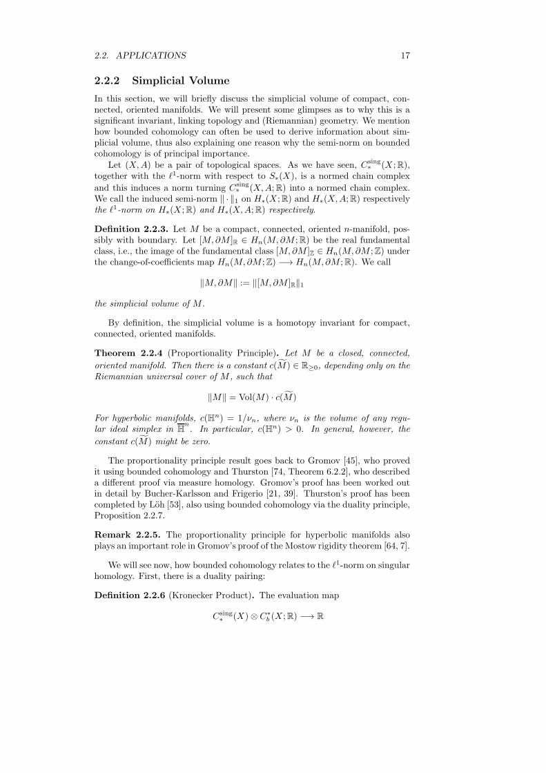
2.2.2 Simplicial Volume
In this section, we will briefly discuss the simplicial volume of compact, con-nected, oriented manifolds. We will present some glimpses as to why this is asignificant invariant, linking topology and (Riemannian) geometry. We mentionhow bounded cohomology can often be used to derive information about sim-plicial volume, thus also explaining one reason why the semi-norm on boundedcohomology is of principal importance.
Let (X,A) be a pair of topological spaces. As we have seen, Csing∗ (X ;R),
together with the ℓ1-norm with respect to S∗(X), is a normed chain complex
and this induces a norm turning Csing∗ (X,A;R) into a normed chain complex.
We call the induced semi-norm ‖ · ‖1 on H∗(X ;R) and H∗(X,A;R) respectivelythe ℓ1-norm on H∗(X ;R) and H∗(X,A;R) respectively.
Definition 2.2.3. Let M be a compact, connected, oriented n-manifold, pos-sibly with boundary. Let [M,∂M ]R ∈ Hn(M,∂M ;R) be the real fundamentalclass, i.e., the image of the fundamental class [M,∂M ]Z ∈ Hn(M,∂M ;Z) underthe change-of-coefficients map Hn(M,∂M ;Z) −→ Hn(M,∂M ;R). We call
‖M,∂M‖ := ‖[M,∂M ]R‖1
the simplicial volume of M .
By definition, the simplicial volume is a homotopy invariant for compact,connected, oriented manifolds.
Theorem 2.2.4 (Proportionality Principle). Let M be a closed, connected,
oriented manifold. Then there is a constant c(M) ∈ R≥0, depending only on theRiemannian universal cover of M , such that
‖M‖ = Vol(M) · c(M)
For hyperbolic manifolds, c(Hn) = 1/νn, where νn is the volume of any regu-lar ideal simplex in H
n. In particular, c(Hn) > 0. In general, however, the
constant c(M) might be zero.
The proportionality principle result goes back to Gromov [45], who provedit using bounded cohomology and Thurston [74, Theorem 6.2.2], who describeda different proof via measure homology. Gromov’s proof has been worked outin detail by Bucher-Karlsson and Frigerio [21, 39]. Thurston’s proof has beencompleted by Loh [53], also using bounded cohomology via the duality principle,Proposition 2.2.7.
Remark 2.2.5. The proportionality principle for hyperbolic manifolds alsoplays an important role in Gromov’s proof of the Mostow rigidity theorem [64, 7].
We will see now, how bounded cohomology relates to the ℓ1-norm on singularhomology. First, there is a duality pairing:
Definition 2.2.6 (Kronecker Product). The evaluation map
Csing∗ (X) ⊗ C∗
b (X ;R) −→ R

18 CHAPTER 2. BOUNDED COHOMOLOGY
induces a well-defined R-map
〈 · , · 〉 : H∗(X ;R) ⊗H∗b (X ;R) −→ R
called the Kronecker product.
By the Hahn-Banach theorem, one gets:
Proposition 2.2.7 (Duality Principle for the ℓ1-Norm, [45, Section 1.1]). Let Xbe a topological space. Then for all α ∈ Hn(X ;R), we get
‖α‖1 = sup
{1
‖ϕ‖∞
∣∣∣∣ ϕ ∈ Hnb (X ;R), 〈α, ϕ〉 = 1
}∪ {0} ∈ R≥0.
Thus, we can use bounded cohomology to study simplical volume [45, 20, 17].
Corollary 2.2.8 ([45, 58, 59]). If the fundamental group of a closed, connected,oriented, aspherical (or more generally: rationally essential) n-manifold M ishyperbolic and n ∈ N≥2, the simplicial volume ‖M‖ is positive.
Proof. Rationally essential implies that the image of the fundamental class [M ]Rof M under the map cn : Hn(M ;R) −→ Hn(Bπ1(M,m);R) induced by theclassifying map is not trivial. Thus, there is a class α ∈ Hn(π1(M,m);R), suchthat 〈cn([M ]R), α〉 = 1. Since π1(M,m) is a hyperbolic group, by Theorem 2.2.2the comparison map Hn
b (π1(M,m);R) −→ Hn(π1(M);R) is surjective, hencethere is also a class β ∈ Hn
b (π1(M);R), such that 〈cn([M ]R), β〉 = 1 and itfollows from the duality principle that ‖M‖ > 0.
Corollary 2.2.9. Let M be a closed, connected, oriented n-manifold, such thatthe fundamental group of M is amenable. Then
‖M‖ = 0.
In general, explicit formulas for non-vanishing simplicial volume are veryrare. As we have seen, the simplicial volume is known (in terms of the vol-ume) for hyperbolic manifolds. It is also additive with respect to certain gluingconstructions along amenable boundaries [45, 72, 18] and, if the dimension isat least 3, with respect to connected sums [45, Section 3.5]. The principal ex-ample not arising from applying these constructions to hyperbolic manifolds isthe calculation of the simplicial volume of manifolds covered by H2 × H2 byBucher-Karlsson:
Theorem 2.2.10 ([21]). Let M be a closed Riemannian manifold, whose Rie-mannian universal cover is isometric to H2 ×H2. Then
‖M‖ =3
2 · π2· Vol(M).
Also in this example, bounded cohomology plays an important part in theproof.

2.2. APPLICATIONS 19
2.2.3 Other Applications
We end this chapter by listing some further applications of bounded cohomology,with no attempt at completeness:
• Various types of superrigidity results [63, 60, 27, 8].
• Generalised Milnor-Wood-type inequalities [23].
• Volume-rigidity for representations of hyperbolic lattices which implies inparticular the Mostow-Prasad rigidity theorem in the case of hyperboliclattices [19].
• Bounded cohomology in degree 2 detects non-trivial quasi-morphisms [37,13, 14].
• Quasi-isometry classification of certain central extensions of Z [42].

20 CHAPTER 2. BOUNDED COHOMOLOGY

Chapter 3
Bounded Cohomology forGroupoids
In this chapter, we introduce bounded cohomology for (pairs of) groupoids. Inthe first section, we recall the definition of groupoids, give some basic examplesand repeat general facts about groupoids. In particular, we discuss the funda-mental groupoid of a topological space, generalising the fundamental group.
In the second section, we present the general setup of homological algebranecessary to deal with the groupoid setting, similar to the group case. Specifi-cally, we consider the Bar resolution and define groupoid (co-)homology, prepar-ing the ground for our definition of bounded cohomology of groupoids.
In the third section, we introduce bounded cohomology and ℓ1-homologywith coefficients for groupoids, generalising the definition for groups, and derivesome fundamental properties of these concepts.
Next, in the fourth section, we develop the setting to deal with boundedcohomology and ℓ1-homology of groupoids via appropriate resolutions. In par-ticular, we discuss the fundamental lemma of homological algebra in this setting.
In the last section, we define bounded cohomology for pairs of groupoids viathe pair of standard resolutions and discuss how other pairs of resolutions canbe used to study bounded cohomology of pairs.
3.1 Groupoids
Groupoids are a generalisation of groups (and group actions), akin to consideringnot necessarily connected spaces in topology. They can be viewed as group-likestructures where composition is only partially defined.
Among many other applications, groupoids arise naturally in topology, e.g.in the form of the fundamental groupoid. This generalisation leads directly toa much more elegant and slightly more powerful treatment of covering theoryand of Van Kampen’s theorem [16, Theorem 6.7.4].
The advantages of the fundamental groupoid here and in other applicationsare that it can be applied also to non-connected spaces and significantly reducesthe dependence on basepoints. These benefits will later be important in ourmain construction.
21

22 CHAPTER 3. BOUNDED COHOMOLOGY FOR GROUPOIDS
Groupoids as a tool have been heavily promoted by Ronald Brown, and wewill follow his outline [16] in this section.
3.1.1 Basic Facts about Groupoids
In this section, we introduce the category of groupoids and some elementaryproperties of them. We also discuss the notion of homotopies between groupoidsand classify groupoids up to homotopy equivalence in terms of their vertexgroups. Furthermore, we give some elementary examples of groupoids.
Definition 3.1.1.
(i) A groupoid is a small category in which every morphism is invertible. Weconsider objects in a groupoid as vertices (in the corresponding graph) andmorphisms as elements of the groupoid and will sometimes use notationsin this spirit. In particular, if G is a groupoid, we will write g ∈ G toindicate that g ∈ ∐e,f∈obG MorG(e, f) is a morphism in G.
(ii) A functor between groupoids is also called a groupoid map.
(iii) A groupoid map is called injective/surjective if it is injective/surjective onboth objects and morphisms.
(iv) A subcategory of a groupoid G which is again a groupoid, is called asubgroupoid of G.
(v) Suppose f, g : G −→ H are groupoid maps. A natural equivalence be-tween f and g is also called a homotopy between f and g. If such ahomotopy exists, we sometimes write f ≃ g.
Note that by the nature of groupoids, such a homotopy h is always invert-ible, an inverse homotopy is given by h := (h−1
e )e∈obG .
(vi) We will write Grp for the category of groupoids with groupoid maps asmorphisms.
Definition 3.1.2.
(i) A groupoid G is called connected, if for each pair i, j ∈ obG there existsat least one morphism from i to j in G (that is, if the underlying graphof the category G is connected). Similarly, we get the notion of connectedcomponents of a groupoid.
(ii) If G is a groupoid, we will write π0(G) ⊂ obG for an (arbitrary) choice ofexactly one vertex in each connected component.
(iii) If e ∈ obG is an object, we call Ge := MorG(e, e) the vertex group of Gat e.
Example 3.1.3.
(i) A group is naturally a groupoid with exactly one object. More precisely,we can (and will) identify the category of groups with the full subcategoryof the category of groupoids, having the vertex set {1}.

3.1. GROUPOIDS 23
(ii) In this sense, the concepts (i) to (iv) in Definition 3.1.1 correspond tothe obvious concepts in the group case. Two group homomorphismsf, g : G −→ H are homotopic if and only if there exists an inner auto-morphism α of H , such that α ◦ f = g.
(iii) Given a family (Gi)i∈I of groupoids, the disjoint union of (Gi)i∈I is thegroupoid ∐i∈IGi, defined by setting ob∐i∈IGi := ∐i∈I obGi and
∀k,l∈I ∀e∈obGk∀f∈obGl
Mor∐i∈IGi(e, f) :=
{MorGk
(e, f) if k = l
∅ else,
together with the composition induced by the compositions of the (Gi)i∈I .In this fashion, we can view a family of groups naturally as a groupoid.
(iv) Let G and H be groupoids. Then G×H, i.e., the category of pairs of objectsand morphisms with componentwise composition, is again a groupoid.
Example 3.1.4. For each set C there is a unique (up to canonical isomorphism)groupoid with object set C and exactly one morphism between each pair ofobjects, called the simplicial groupoid with vertex set C. For each n ∈ N, wewrite ∆n for the simplicial groupoid with vertex set {0, . . . , n}.
Example 3.1.5 (Group Actions and Groupoids). Let G be a group and X aset with a left G-action. We define a groupoid G⋉X , called the action groupoidor the semi-direct product of X and G, by setting:
(i) The objects of G⋉X are given by obG⋉X = X .
(ii) For each e, f ∈ X , set MorG⋉X(e, f) = {(e, g) ∈ X ×G | g · e = f}.
(iii) Define the composition by setting for each x ∈ X and g, h ∈ G
(g · x, h) ◦ (x, g) = (x, h · g).
We will view groupoids as groups where the composition is only partiallydefined, in the sense that we can only compose two elements if the target of thefirst matches the source of the second. Thus it will be useful to define:
Definition 3.1.6. Let G be a groupoid. We define a map
s : G −→ obG
MorG(e, f) ∋ g 7−→ e
called source and a map
t : G −→ obG
MorG(e, f) ∋ g 7−→ f.
called target.
As the next theorem shows, up to homotopy we can actually always restrictto disjoint families of groups:

24 CHAPTER 3. BOUNDED COHOMOLOGY FOR GROUPOIDS
Theorem 3.1.7 (Classifying groupoids up to homotopy). Let G be a groupoidand i : H −→ G be the inclusion of a full subgroupoid meeting each connectedcomponent of G. Then there exists a groupoid map p : G −→ H, such that
p ◦ i = idH and i ◦ p ≃ idG .
In particular, H and G are equivalent.
Proof. Choose a set-theoretic section α : obG −→ obH of obH −→ obG thatmaps vertices to vertices in the same connected component of G. Then choosea map e : obG −→ MorG such that
∀v∈obG e(v) ∈ HomG(v, α(v)) and ∀v∈obH e(v) = idv ∈ HomG(v, v).
Finally, define a groupoid map p : G −→ H by
∀v∈obG p(v) = α(v)
∀v,w∈obG ∀σ∈HomG(v,w) p(σ) = e(w) ◦ σ ◦ e(v)−1 ∈ HomH(α(v), α(w)).
We immediately see that this map is functorial and that p ◦ i = idH. Byconstruction, e is a natural equivalence between i ◦ p and idG .
Corollary 3.1.8.
(i) Two groupoids H and G are equivalent if and only if there is a bijectionα : π0G −→ π0H, such that for all e ∈ π0G the vertex groups Ge and Hα(e)
are isomorphic.
(ii) In particular: Every connected non-empty groupoid is equivalent to anyof its vertex groups (which coincide up to isomorphism).
Proof. Let ϕ := (ϕe : Ge −→ Hα(e))e∈π0(G) be a family of group isomorphisms.Then ϕ induces an isomorphism ∐e∈π0(G)Ge −→ ∐e∈π0(H)He and hence
G ≃ ∐e∈π0(G)Ge∼= ∐e∈π0(H)He ≃ H.
The next proposition motivates the term “homotopy” for a natural equiva-lence:
Proposition 3.1.9. Let f0, f1 : G −→ H be groupoid maps. Consider the twocanonical inclusion maps µ0, µ1 : G −→ G × ∆1 given by
∀i∈obG µt(i) = (i, t)
∀g∈morG µt(g) = (g, idt)
for t ∈ {0, 1}. Then there is a one-to-one correspondence between the ho-motopies from f0 to f1 and the groupoid maps H : G × ∆1 −→ H satisfy-ing H ◦ µ0 = f0 and H ◦ µ1 = f1.

3.1. GROUPOIDS 25
Proof. Let e01, e10 denote the two non-trivial morphisms in ∆1. If H : G ×∆1 −→ H is a groupoid map satisfying H ◦µ0 = f0 and H ◦µ1 = f1, by settingfor each e ∈ obG
he := H(ide, e01) : f0(e) −→ f1(e)
we get a homotopy from f0 to f1, since for each pair e, e′ ∈ obG and eachmorphism α ∈ HomG(e, e′)
he′ ◦ f0(α) = H(ide′ , e01) ◦H(α, id0)
= H(α, id1) ◦H(ide, e01)
= f1(α) ◦ he.
On the other hand, if h is a homotopy from f0 to f1, we can define a groupoidmap H : G × ∆1 −→ H satisfying H ◦ µ0 = f0 and H ◦ µ1 = f1 by setting
∀(i,t)∈obG×∆1 H(i, t) = ft(i)
∀g∈mor G H(g, id0) = f0(g) H(g, id1) = f1(g)
H(ide, e01) = he H(ide, e10) = h−1e .
We give a last example that shows that for each set of vertices and eachgroup, we can “blow up” this group to get a groupoid homotopy equivalent tothe group having the given vertex set. This will be useful later when we wantto consider a group G together with a family of subgroups (Ai)i∈I as a pair ofgroupoids, e.g., by considering (GI ,∐i∈IAi).
Definition 3.1.10. Let G be a group and C a set. We define a groupoid GC
by setting
• Objects: obGC := C.
• Morphisms: ∀e,f∈C MorGC(e, f) := G.
We then define composition by multiplication of elements in G, i.e., by settingfor all d, e, f ∈ C
MorGC(e, f) × MorGC
(d, e) −→ MorGC(d, f)
(g, h) 7−→ g · h.
Example 3.1.11. For each set C, we see that {1}C is the simplicial groupoidwith vertex set C.
3.1.2 The Fundamental Groupoid
For us, the main examples of groupoids, besides (disjoint families of) groups, willbe given by fundamental groupoids of topological spaces. These are straightfor-ward generalisations of the fundamental group:
26 CHAPTER 3. BOUNDED COHOMOLOGY FOR GROUPOIDS
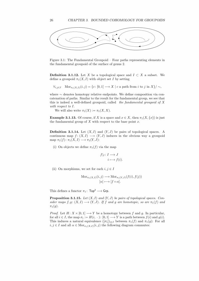
Figure 3.1: The Fundamental Groupoid – Four paths representing elements inthe fundamental groupoid of the surface of genus 2.
Definition 3.1.12. Let X be a topological space and I ⊂ X a subset. Wedefine a groupoid π1(X, I) with object set I by setting
∀i,j∈I Morπ1(X,I)(i, j) = {c : [0, 1] −→ X | c a path from i to j in X}/ ∼,
where ∼ denotes homotopy relative endpoints. We define composition via con-catenation of paths. Similar to the result for the fundamental group, we see thatthis is indeed a well-defined groupoid, called the fundamental groupoid of Xwith respect to I.
We will also write π1(X) := π1(X,X).
Example 3.1.13. Of course, if X is a space and x ∈ X , then π1(X, {x}) is justthe fundamental group of X with respect to the base point x.
Definition 3.1.14. Let (X, I) and (Y, J) be pairs of topological spaces. Acontinuous map f : (X, I) −→ (Y, J) induces in the obvious way a groupoidmap π1(f) : π1(X, I) −→ π1(Y, J):
(i) On objects we define π1(f) via the map
f |I : I −→ J
i 7−→ f(i).
(ii) On morphisms, we set for each i, j ∈ I
Morπ1(X,I)(i, j) −→ Morπ1(Y,J)(f(i), f(j))
[α] 7−→ [f ◦ α].
This defines a functor π1 : Top2 −→ Grp.
Proposition 3.1.15. Let (X, I) and (Y, J) be pairs of topological spaces. Con-sider maps f, g : (X, I) −→ (Y, J). If f and g are homotopic, so are π1(f) andπ1(g).
Proof. Let H : X × [0, 1] −→ Y be a homotopy between f and g. In particular,for all i ∈ I, the map σi := H(i, · ) : [0, 1] −→ Y is a path between f(i) and g(i).This induces a natural equivalence ([σi])i∈I between π1(f) and π1(g): For alli, j ∈ I and all α ∈ Morπ1(X,I)(i, j) the following diagram commutes:
3.2. HOMOLOGICAL ALGEBRA FOR GROUPOIDS 27
f(i) g(i)
f(j) g(j)
[σi]
[f ◦ α]
[σj ]
[g ◦ α]
Here [σi ∗ (f ◦ α)] = [(g ◦ α) ∗ σj ] holds via the given homotopy.
3.2 Homological Algebra for Groupoids
In this section, we will discuss the algebraic setup to treat (co-)homology forgroupoids, preparing the ground for our definition of bounded cohomology inthe later sections. We introduce groupoid modules and generalise several alge-braic constructions into this context. We then discuss the Bar resolution forgroupoids, define groupoid (co-)homology with coefficients and prove some el-ementary properties. The Bar resolution and the corresponding definition ofcohomology is a straightforward generalisation of the group case and has beenextensively studied also for groupoids, for instance [71, 75].
3.2.1 Groupoid Modules
In this section we will present our definition of a module over a groupoid, gener-alising the group case. We will then translate basic concepts for group modules,e.g. (co-)invariants, quotients etc., to this setting. Since we are mainly in-terested in bounded cohomology, we will restrict ourselves to real coefficients,though we could as well work with arbitrary coefficient rings.
Definition 3.2.1 (Groupoid modules). Let G be a groupoid. A (left) G-moduleV = (Ve)e∈ob G consists of:
(i) A family of real vector spaces (Ve)e∈ob G .
(ii) A partial action of G on V , i.e. for each g ∈ G a linear map
ρg : Vs(g) −→ Vt(g)
v 7−→ ρg(v) =: gv,
such that:
(a) For all g, h ∈ G with s(g) = t(h) we have ρg ◦ ρh = ρgh.
(b) For all i ∈ obG we have ρidi= idVi
.
Definition 3.2.2 (G-maps). Let G be a groupoid.
(i) Let V and W be G-modules. An R-morphism between V and W is afamily (fe : Ve −→We)e∈ob G of R-linear maps.
(ii) Let f : V −→ W be an R-morphism between G-modules. We call fa G-map or G-equivariant, if for all g ∈ G we have ρWg ◦ fs(g) = ft(g) ◦ ρ
Vg .

28 CHAPTER 3. BOUNDED COHOMOLOGY FOR GROUPOIDS
(iii) We write G-Mod for the category of G-modules and G-maps.
Remark 3.2.3. By definition, a left G-module is nothing else than a covariantfunctor G −→ R-Mod. In this sense, a G-map is just a natural transformationbetween such functors.
The functorial point of view is elegant, but the definition in terms of partialactions is more concrete and in direct analogy to the usual point of view in thegroup case. The latter definition will be our guide in the following sections,though we will also use the functorial definition to define some concepts moreconcisely.
Definition 3.2.4 (The trivial G-module). Let G be a groupoid. Consider themodule R[G] := (Re)e∈obG = (R)e∈ob G . We will always endow this module withthe trivial G action given by
ρg = idR : Rs(g) −→ Rt(g)
for all g ∈ G.
We will see more examples in later sections. In the remainder of this section,we will translate the basic concepts of group modules into the groupoid setting,concepts that we will need later in order to do homological algebra.
Definition 3.2.5. Let A and G be groupoids and let f : A −→ G be a groupoidmap.
(i) Let U : G −→ R-Mod be a G-module. We call the A-module f∗U := U ◦ fthe induced A-module structure on U .
(ii) Let ϕ : U −→ V be a G-morphism. We define an A-morphism
f∗ϕ : f∗U −→ f∗V,
by setting ((f∗ϕ)e)e∈obA = (ϕf(e))e∈obA. This defines a functor
f∗ : G-Mod −→ A-Mod .
Lemma 3.2.6. Let G and H be groupoids and let V be an H-module. Letf0, f1 : G −→ H be groupoid maps and h a homotopy between f0 and f1. Then
V ◦ h : f∗0V −→ f∗
1V
Vf0(e) ∋ v 7−→ he · v
is a G-isomorphism.We will also use a multiplicative notation and write h ·v to denote (V ◦h)(v).
Proof. By Remark 3.2.3, V ◦h is a G-map. Its inverse is given by V ◦h, where hdenotes the inverse homotopy to h.
Definition 3.2.7. Let G be a groupoid and let V and W be G-modules. Weset
Hom(V,W ) = {f : V −→W | f is an R-morphism of G-modules}
There is a canonical G-structure on Hom(V,W ) given by:

3.2. HOMOLOGICAL ALGEBRA FOR GROUPOIDS 29
(i) Hom(V,W ) = (Hom(Ve,We))e∈obG .
(ii) For all g ∈ G and f ∈ Hom(Vs(g),Ws(g)) we define g ·f ∈ Hom(Vt(g),Wt(g))by setting
∀v∈Vt(g)(g · f)(v) = g · f(g−1 · v).
Remark 3.2.8. Another way to see this is to view Hom(V,W ) as the compo-sition
G (R-Mod)2 R-Mod,(V,W ) Hom
where W is the contravariant functor given by inverting morphisms in G andthen applying W .
Remark 3.2.9. Let G be a groupoid. Let f : V −→ W be a G-map and Ca G-module. Then the dual map Hom(f, C) : Hom(W,C) −→ Hom(V,C) (cor-responding to the family (Hom(fe, Ce))e∈ob G) is again a G-map. Alternatively,we can view Hom(f, C) also as the composition of the natural transformationbetween (V,C) and (W,C) induced by f and the functor Hom.
This gives rise to a contravariant functor Hom( · , C) : G-Mod −→ G-Mod.
Proof. The map Hom(f, C) is G-equivariant since for all g ∈ G, all v ∈ Vt(g) andall α ∈ Hom(Ws(g), Cs(g))
Hom(f, C)(gα)(v) = (gα)(f(v))
= g(α(g−1f(v)))
= g(α(f(g−1v)))
= g(α ◦ f)(v)
= g(Hom(f, C)(α))(v).
Definition 3.2.10 (Tensor products). Let G be a groupoid and let V and Wbe G-modules. We define the tensor product of V and W over R to be the G-module V ⊗W = (Ve⊗We)e∈obG with the induced G-structure given by settingfor each g ∈ G
ρg : Vs(g) ⊗Ws(g) −→ Vt(g) ⊗Wt(g)
v ⊗ w 7−→ (g · v) ⊗ (g · w).
In other words, V ⊗W is the composition
G (R-Mod)2 R-Mod .(V,W ) ⊗
Definition 3.2.11 (Coinvariants and Invariants). Let G be a groupoid andlet V be a G-module.
(i) We define the coinvariants of V to be the quotient module
VG =⊕
e∈obG
Ve/〈v − g · v | g ∈ G, v ∈ Vs(g)〉.
30 CHAPTER 3. BOUNDED COHOMOLOGY FOR GROUPOIDS
This construction gives rise to a functor G-Mod −→ R-Mod by setting foreach G-map α : V −→W
αG : VG −→WG
[v] 7−→ [α(v)].
In other words, the coinvariants of V are just the canonical model for thecolimit of V : G −→ R-Mod, [76, Propostion 2.6.8].
(ii) We define the invariants of V to be the R-subspace V G of∏
e∈obG Vedefined as
V G ={v ∈
∏
e∈obG
Ve
∣∣∣ ∀g∈G g · vs(g) = vt(g)
}.
This construction gives rise to a functor G-Mod −→ R-Mod by setting foreach G-map α : V −→W
αG : V G −→WG
(ve)e∈ob G 7−→ (α(ve))e∈ob G .
In other words, the invariants of V are just the canonical model for thelimit of V : G −→ R-Mod, [76, Propostion 2.6.9].
Definition 3.2.12. Let G be a groupoid and V and W be G-modules. We call
V ⊗G W := (V ⊗W )G
the tensor product of V and W over G. This construction gives rise to a func-tor · ⊗G W : G-Mod −→ R-Mod by setting for each G-map α : U −→ U ′
α⊗W : U ⊗G W −→ U ′ ⊗G W
[u⊗ w] 7−→ [α(u) ⊗ w].
Definition 3.2.13. Let G be a groupoid and let V and W be G-modules. Thenwe set
HomG(V,W ) := Hom(V,W )G .
This induces a contravariant functor HomG( · ,W ) : G-Mod −→ R-Mod.
Definition 3.2.14 (G-Submodules). Let G be a groupoid and let V be a G-module. A G-submodule of V is a family (We)e∈ob G of real vector spaces suchthat
(i) For each e ∈ obG the space We is a subspace of Ve.
(ii) For all g ∈ Gg ·Ws(g) ⊂Wt(g).
Then W carries a G-module structure by considering the restricted G-action.
Example 3.2.15. Let f : V −→W be a G-map. Then its image (fe(Ve))e∈ob G
is a G-submodule of W .

3.2. HOMOLOGICAL ALGEBRA FOR GROUPOIDS 31
Definition 3.2.16. Let G be a groupoid and α : V −→ W be a G-map. Thenwe call
kerα := (kerαe)e∈obG
the kernel of α. Clearly, kerα is a G-submodule of V .
Proposition 3.2.17 (Quotients). Let G be a groupoid, let B be a G-moduleand A a G-submodule of B. Then there exists a canonical G-module structureon B/A = (Be/Ae)e∈ob G such that the family of canonical projections π =(πe : Be −→ Be/Ae)e∈obG is a G-map with the following universal property:Assume that C is a G-module and f : B −→ C a G-map such that fe(Ae) =0 for all e ∈ obG. Then there exists a unique G-map f : B/A −→ C suchthat f ◦ π = f .
Proof.
• For all g ∈ G, we have g · As(g) ⊂ At(g), hence there is a unique linearmap ρg making the following diagram commutative:
Bs(g) Bt(g)
Bs(g)/As(g) Bt(g)/At(g)
ρg
ρg
πt(g)πs(g)
This induces a G-structure on B/A.
• The projection π : B −→ B/A is a G-map by the definition of ρg.
• There exists a unique family of linear maps f = (fe : Be −→ Be/Ae)e∈ob G
such that fe ◦ πe = fe for all e ∈ obG. This map is a G-map since forall g ∈ G
ft(g) ◦ ρg ◦ πs(g) = ft(g) ◦ πt(g) ◦ ρg
= ft(g) ◦ ρg
= ρg ◦ fs(g)
= ρg ◦ fs(g) ◦ πs(g).
So f is G-equivariant.
Remark 3.2.18. The notions of chain complex, chain contraction, resolutionand so on, easily translate into the setting of groupoid modules.
Also, it is easy to see that G-Mod is an Abelian category ([76, DefinitionA4.2]).
3.2.2 The Bar Resolution
In this section, we will define the Bar resolution for groupoids, extending thedefinition for the group case. We will also present a homogeneous version andshow that these two resolutions are chain isomorphic. Finally, we will introducethe Bar (co-)complex with coefficients in groupoid modules, too.

32 CHAPTER 3. BOUNDED COHOMOLOGY FOR GROUPOIDS
Definition 3.2.19 (The Bar resolution for groupoids). Let G be a groupoid.
(i) For each n ∈ N, we set
Pn(G) = {(g0, . . . , gn) ∈ Gn+1 | ∀i∈{0,...,n−1} s(gi) = t(gi+1)}.
Equivalently, Pn(G) is the set of all (n+ 1)-paths in G.
(ii) For all e ∈ obG consider
Cn(G)e = R〈{(g0, . . . , gn) ∈ Pn(G) | t(g0) = e}〉.
We define a sequence of R-modules (Cn(G))n∈N by setting for all n ∈ N
Cn(G) = (Cn(G)e)e∈ob G
These modules carry a canonical G-structure. The G-action is then givenby setting for all g ∈ G
ρg : Cn(G)s(g) −→ Cn(G)t(g)
(g0, . . . , gn) 7−→ (g · g0, . . . , gn).
(iii) For each n ∈ N, we define boundary maps
∂n : Cn(G) −→ Cn−1(G)
(g0, . . . , gn) 7−→n−1∑
i=0
(−1)i(g0, . . . , gi · gi+1, . . . , gn)
+ (−1)n · (g0, . . . , gn−1).
These are obviously G-maps.
(iv) The usual calculation shows that this does indeed define a G-chain com-plex (Cn(G), ∂n)n∈N.
Remark 3.2.20. Let G be a groupoid. Consider the canonical augmentationmap
ε : C0(G) −→ R[G]
g 7−→ t(g) · 1.
Then (Cn(G), ∂n)n∈N together with ε is a G-resolution of R[G]. An R-chaincontraction s∗ is given by the R-morphisms
s−1 : R[G] −→ C0(G)
e 7−→ ide
and for all n ∈ N
sn : Cn(G) −→ Cn+1(G)
(g0, . . . , gn) 7−→ (idt(g0), g0, . . . , gn).

3.2. HOMOLOGICAL ALGEBRA FOR GROUPOIDS 33
Remark 3.2.21. The set P (G) := ∐n∈NPn(G) is just the underlying set of thenerve of the category G. Therefore (Pn(G))n∈N is a simplicial set with the usualboundary maps
∂i,n : Pn(G) −→ Pn−1(G)
(g0, . . . , gn) 7−→ (g0, . . . , gi · gi+1, . . . , gn)
for each n ∈ N>0 and i ∈ {0, . . . , n} and degeneracy maps
si,n : Pn(G) −→ Pn+1(G)
(g0, . . . , gn) 7−→ (g0, . . . , gi, ids(gi), gi+1, . . . , gn).
for each n ∈ N and i ∈ {0, . . . , n}. Taking the G-action into account, we couldview P (G) as a functor P (G) : G −→ sSet. The chain complex C∗(G) can thenbe viewed as the usual chain complex associated to a simplicial set (but overthe groupoid G.) We refer the book of May [55] for more on simplicial sets.
As in the group case, it is sometimes helpful to use a homogeneous resolutionchain isomorphic to the Bar resolution:
Definition 3.2.22 (The homogeneous Bar resolution). Let G be a groupoid.
(i) For each n ∈ N, we define a G-module Ln(G) by setting for each e ∈ obG
Ln(G)e = R〈{(g0, . . . , gn) ∈ Gn+1 | ∀i∈{0,...,n} t(gi) = e}〉.
and defining a G-action by setting for each g ∈ G
ρg : Ln(G)s(g) −→ Ln(G)t(g)
(g0, . . . , gn) 7−→ (g · g0, . . . , g · gn).
(ii) For each n ∈ N, we define boundary maps
∂n : Ln(G) −→ Ln−1(G)
(g0, . . . , gn) 7−→n∑
i=0
(−1)i(g0, . . . , gi, . . . , gn).
These are obviously G-maps.
(iii) The usual calculation shows that this does indeed define a G-chain com-plex (Ln(G), ∂n)n∈N.
Proposition 3.2.23. The maps
Cn(G) −→ Ln(G)
(g0, . . . , gn) 7−→ (g0, g0 · g1, . . . , g0 · · · · gn)
and
Ln(G) −→ Cn(G)
(g0, . . . , gn) 7−→ (g0, g−10 · g1, . . . , g
−1n−1 · gn)
are well-defined, mutually inverse G-chain isomorphisms.

34 CHAPTER 3. BOUNDED COHOMOLOGY FOR GROUPOIDS
Proof. The maps are obviously mutually inverse G-maps in each degree. Theyare chain maps by the same calculation as in the group case, [47, Section VI.13].
Remark 3.2.24. If G is a group, then C∗(G) and L∗(G) coincide with the usualdefinition of the (homogeneous) real Bar resolution of the group G.
Definition 3.2.25 (Functoriality). Let f : A −→ G be a groupoid map. Thenthe induced map
(Cn(f) : Cn(A) −→ Cn(G)
(a0, . . . , an) 7−→ (f(a0), . . . , f(an))
)
n∈N
is an A-chain map with respect to the induced A-structure on C∗(G).
In order to study (bounded) (co-)homology with coefficients, it will be usefulto define a domain category that encompasses both groupoids and coefficientmodules. We follow Kenneth Brown [15, Section III.8] here:
Definition 3.2.26 (Domain categories for (co-)homology).
(i) We define a category GrpMod by setting:
(a) Objects in GrpMod are pairs (G, V ), where G is a groupoid and V isa G-module.
(b) A morphism (G, V ) −→ (H,W ) in GrpMod is a pair (f, ϕ), wheref : G −→ H is a groupoid map and ϕ : V −→ f∗W is a G-map.
(c) Composition is defined by setting for all composable pairs of mor-phisms (f, ϕ) : (G, V ) −→ (H,W ) and (g, ψ) : (H,W ) −→ (A, U):
(g, ψ) ◦ (f, ϕ) := (g ◦ f, (f∗ψ) ◦ ϕ).
(ii) We define a category GrpMod by setting:
(a) Objects in GrpMod are pairs (G, V ), where G is a groupoid and V isa G-module.
(b) A morphism (G, V ) −→ (H,W ) in GrpMod is a pair (f, ϕ), wheref : G −→ H is a groupoid map and ϕ : f∗W −→ V is a G-map.
(c) Composition is defined by setting for all composable pairs of mor-phisms (f, ϕ) : (G, V ) −→ (H,W ) and (g, ψ) : (H,W ) −→ (A, U):
(g, ψ) ◦ (f, ϕ) := (g ◦ f, ϕ ◦ (f∗ψ)).
Definition 3.2.27 (Bar Complex with Coefficients). Let G be a groupoid and Va G-module.
(i) We write
C∗(G;V ) := C∗(G) ⊗G V.
Together with ∂∗ ⊗ idV , this is an R-chain complex.

3.2. HOMOLOGICAL ALGEBRA FOR GROUPOIDS 35
(ii) If (f, ϕ) : (G, V ) −→ (H,W ) is a morphism in GrpMod, we write
C∗(f ;ϕ) := i ◦ (C∗(f) ⊗G ϕ) : C∗(G;V ) −→ C∗(H;W )
x⊗ v 7−→ f(x) ⊗ ϕ(v).
Here, let i denote the canonical R-map
i : f∗C∗(H) ⊗G f∗W −→ C∗(H) ⊗H W
v ⊗ w 7−→ v ⊗ w.
This defines a functor C∗( · , · ) : GrpMod −→ RCh.
(iii) If f : G −→ H is a groupoid map and W an H-module, we also write
C∗(f ;W ) := C∗(f ; idf∗W ).
(iv) We writeC∗(G;V ) := HomG(C∗(G), V ).
Together with δ∗ := HomG(∂∗+1, V ), this is an R-cochain complex.
(v) If (f, ϕ) : (G, V ) −→ (H,W ) is a morphism in GrpMod, we write C∗(f ;ϕ)for the map
HomG(C∗(f), ϕ) ◦ j : C∗(H;W ) −→ C∗(G;V )
(we)f∈obH 7−→ (ϕ ◦ wf(e) ◦ C∗(f))e∈ob G .
Here, let j denote the canonical R-map
j : HomH(C∗(H),W ) −→ HomG(f∗C∗(H), f∗W )
(ve)e∈obH 7−→ (vf(e))e∈ob G .
This defines a contravariant functor C∗( · , · ) : GrpMod −→ RCh.
(vi) If f : G −→ H is a groupoid map and W an H-module, we also write
C∗(f ;W ) := C∗(f ; idf∗W ).
3.2.3 (Co-)homology
In this section, we will introduce (co-)homology for groupoids with coefficientsin groupoid modules, extending the definition in the group case. We will seethat it is a groupoid homotopy invariant and can thus be calculated directly viagroup homology of vertex groups. For an overview of group homology, we referto the literature [15, 47, 76].
Definition 3.2.28. Let G be a groupoid and V a G-module.
(i) We callH∗(G;V ) := H∗
(C∗(G;V )
)
the homology of G with coefficients in V . As usual, H∗
(C∗(G;V )
)denotes
the homology of the R-chain complex C∗(G;V ).
This defines a functor H∗ : GrpMod −→ R-Mod∗.
36 CHAPTER 3. BOUNDED COHOMOLOGY FOR GROUPOIDS
(ii) We callH∗(G;V ) := H∗
(C∗(G;V )
)
the cohomology of G with coefficients in V . Here, H∗(C∗(G;V )
)denotes
the cohomology of the R-cochain complex C∗(G;V ).
This defines a contravariant functor H∗ : GrpMod −→ R-Mod∗.
Remark 3.2.29. If G is a group, these definitions coincide with the usualdefinitions of group (co-)homology.
Proposition 3.2.30. Let G and H be groupoids. Let f0, f1 : G −→ H begroupoid maps and let h be a homotopy from f1 to f0.
(i) For each n ∈ N and each i ∈ {0, . . . , n} define a G-map
sin : Cn(G) −→ f∗0Cn+1(H)
(g0, . . . , gn) 7−→ (f0(g0), . . . , f0(gi), hs(gi), f1(gi+1), . . . , f1(gn)).
Define for each n ∈ N a G-map
sn :=
n∑
i=0
(−1)isin.
Then ∂n+1 ◦ sn + sn−1 ◦ ∂n = Cn(f0) − h · Cn(f1) for each n ∈ N, i.e., s∗is a G-chain homotopy between C∗(f0) and h · C∗(f1).
(ii) Let V be an H-module. Then
sV∗ := i ◦ (s∗ ⊗G idf∗0 V ) : C∗(G; f∗
0 V ) −→ C∗+1(H;V )
x⊗ v 7−→ s∗(x) ⊗ v
is an R-chain homotopy between C∗(f0;V ) and C∗(f1;V ◦ h).
(iii) In particular,
H∗(f0;V ) = H∗(f1;V ◦ h) = H∗(f1;V ) ◦H∗(idG ;V ◦ h);
and the map H∗(idG ;V ◦ h) is an isomorphism.
(iv) Dually,
s∗V := (HomG(s∗, idf∗0 V )) ◦ j : C∗(H, V ) −→ C∗−1(G; f∗
0V )
(we)e∈obH 7−→ (wf0(e) ◦ s∗,e)e∈ob G .
is an R-cochain homotopy between C∗(f0;V ) and C∗(f1;V ◦ h).
(v) In particular,
H∗(f0;V ) = H∗(f1;V ◦ h) = H∗(idG ;V ◦ h) ◦H∗(f1;V );
and the map H∗(idG ;V ◦ h) is an isomorphism.
Proof.

3.2. HOMOLOGICAL ALGEBRA FOR GROUPOIDS 37
(i) Obviously, for each n ∈ N and i ∈ {0, . . . , n} the map sin is G-equivariant.The sin define a homotopy P (G) −→ P (H) of simplicial sets between P (f0)and h · P (f1), see Remark 3.2.31, hence they induce a homotopy be-tween C∗(f0) and h · C∗(f1). Alternatively, this can be seen by a shortcalculation.
(ii) We have for each e ∈ obG, each x ∈ Cn(G)e and each v ∈ Vf0(e)
(∂n+1sVn + sVn−1∂n)(x ⊗ v) = (∂n+1sn(x) + sn−1∂n(x)) ⊗ v.
= Cn(f0)(x) ⊗ v − he · Cn(f1)(x) ⊗ v
= Cn(f0)(x) ⊗ v − Cn(f1)(x) ⊗ h−1e · v
= Cn(f0;V )(x⊗ v) − Cn(f1;V ◦ h)(x⊗ v).
(iii) The map H∗(idG ;V ◦ h) is an isomorphism by Lemma 3.2.6.
The parts (iv) and (v) are dual to parts (ii) and (iii).
Remark 3.2.31. Again, it is useful to also consider a simplicial point of view.The family (sin)i,n is directly seen to be a simplicial homotopy (over G) be-tween P (f0) and h · P (f1).
Corollary 3.2.32. Let f : G −→ H be a homotopy equivalence between grou-poids and V an H-module. Then the induced maps
H∗(f ;V ) : H∗(G; f∗V ) −→ H∗(H;V )
and
H∗(f ;V ) : H∗(H;V ) −→ H∗(G; f∗V )
are isomorphisms of graded R-modules.
Corollary 3.2.33 (Group cohomology calculates groupoid cohomology). Let Gbe a connected groupoid and V a G-module. Let e ∈ obG be a vertex andlet ie : Ge −→ G be the inclusion of the corresponding vertex group. Then
H∗(ie;V ) : H∗(Ge, i∗eV ) −→ H∗(G;V )
and
H∗(ie;V ) : H∗(G, V ) −→ H∗(Ge; i∗eV )
are isomorphisms of graded R-modules.
Proof. By Corollary 3.1.8, ie is a homotopy equivalence and by Corollary 3.2.32,the induced maps are isomorphisms.
Similar to the situation for topological spaces, groupoid (co-)homology isadditive with respect to connected components of groupoids:

38 CHAPTER 3. BOUNDED COHOMOLOGY FOR GROUPOIDS
Proposition 3.2.34 (Groupoid (co-)homology and disjoint unions). Let G bea groupoid and V a G-module. Let G = ∐λ∈ΛGλ be the partition of G intoconnected components. For each λ ∈ Λ, write V λ for the Gλ-module struc-ture on V induced by the inclusion Gλ −→ G. Then the family of canonicalinclusions (Gλ −→ G)λ∈Λ induces isomorphisms
⊕
λ∈Λ
H∗(Gλ;V λ) −→ H∗(G;V )
and
H∗(G;V ) −→∏
λ∈Λ
H∗(Gλ;V λ).
Proof. Clearly, each path in G is contained in a single connected componentof G. Thus we get a corresponding splitting of C∗(G) which is compatible withthe boundary maps and preserved after applying ⊗GV and HomG( · , V ).
Remark 3.2.35. Combining Proposition 3.2.34 with Corollary 3.2.33, we cancalculate groupoid (co-)homology completely in terms of group (co-)homology.
Example 3.2.36. Let X be a topological space. Let Λ ⊂ X be a subsetcontaining exactly one point for each connected component of X . Then thefamily of inclusions (π1(X, x) −→ π1(X))x∈Λ induces isomorphisms of gradedR-modules
⊕
x∈Λ
H∗(π1(X, x);R) −→ H∗(π1(X);R[π1(X)])
and
H∗(π1(X);R[π1(X)]) −→∏
x∈Λ
H∗(π1(X, x);R).
3.3 Bounded Cohomology for Groupoids
We will now define bounded cohomology and ℓ1-homology for groupoids andderive some elementary properties.
3.3.1 Banach G-Modules
In this section, we develop the algebraic setting to study bounded cohomologyand ℓ1-homology, introducing Banach modules over groupoids. Furthermore,we introduce bounded maps and the projective tensor product in this setting.
Definition 3.3.1 (Banach G-Modules). Let G be a groupoid.
(i) A normed G-module is a family of normed real vector spaces (Ve, ‖·‖)e∈obG
together with a G-structure on (Ve)e∈ob G such that
∀g∈G ∀v∈Vs(g)‖g · v‖ = ‖v‖;
i.e., the maps ρg : Vs(g) −→ Vt(g) are isometries for all g ∈ G.

3.3. BOUNDED COHOMOLOGY FOR GROUPOIDS 39
Equivalently, a normed G-module is a functor G −→ R-Mod1‖·‖, where
we denote by R-Mod1‖·‖ the category of normed R-modules together withnorm-non increasing linear maps.
(ii) We call a normed G-module V a Banach G-module if for each e ∈ obG,the normed R-module (Ve, ‖ · ‖) is in addition a Banach space.
(iii) Let V and W be normed G-modules. We call a G-map f : V −→ Wbounded if fe is bounded for each e ∈ obG and the supremum ‖f‖∞ :=supe∈obG ‖fe‖∞ exists. We will now always assume that maps betweennormed G-modules are bounded.
(iv) This defines a category G-Mod‖·‖ of normed G-modules and bounded G-maps.
Example 3.3.2. Let (V, ‖ · ‖V ) and (W, ‖ · ‖W ) be normed G-modules. Thenthe family
B(V,W ) := (B(Ve,We))e∈ob G
is a G-subspace of Hom(V,W ). Here, B(Ve,We) denotes the space of boundedlinear functions from Ve to We. It is a normed G-space with respect to thefamily of operator norms ‖ · ‖∞ induced by the families of norms on V and W .If W is a Banach G-module, so is B(V,W ). This is functorial with respect tobounded G-maps.
Proof. For all g ∈ G, all f ∈ Hom(Vs(g),Ws(g)) and all v ∈ Vt(g) we have
∥∥(gf)(v)∥∥W
= ‖gf(g−1v)‖W = ‖f(g−1v)‖W .
Hence gf is bounded if f is bounded, so gB(Vs(g),Ws(g)) ⊂ B(Vt(g),Wt(g)). Inthis case we get by the same calculation
‖gf‖∞ = supv∈Vt(g)\{0}
‖v‖−1V ‖f(g−1v)‖W
≤ supv∈Vt(g)\{0}
‖v‖−1V ‖f‖∞‖g−1v‖V
= ‖f‖∞.
And equality follows because the same is true for g−1. Hence, the action isisometric.
Remark 3.3.3. Alternatively, we can view B(V,W ) as the composition
G (R-Mod‖·‖)2 R-Mod‖·‖,(V,W ) B
where W is the contravariant functor given by inverting morphisms in G andthen applying W .
We will need a normed version of invariants of a G-Banach module V , slightlydifferent from the definition in Section 3.2.1 and by a slight abuse of notation,we will denote these also with V G :

40 CHAPTER 3. BOUNDED COHOMOLOGY FOR GROUPOIDS
Definition 3.3.4. Let V = (Ve, ‖ · ‖e)e∈ob G be a normed G-module. We callthe R-submodule of
∏e∈obG Ve
V G :={v ∈
∏
e∈obG
Ve
∣∣∣ ∀g∈G g · vs(g) = vt(g), supe∈obG
‖ve‖e <∞},
endowed with the norm given by setting for each v ∈ V G
‖v‖ := supe∈obG
‖ve‖e
the (normed) invariants of V .(This can also be seen as the canonical model for the limit of V : G −→
R-Mod1‖·‖).
If G has only finitely many connected components, this definition coincideswith Definition 3.2.11. This is functorial with respect to bounded G-maps:
Proposition 3.3.5. This defines a functor
( · )G : G-Mod‖·‖ −→ R-Mod‖·‖ .
One important example of this construction will be BG(V,W ) := B(V,W )G .
Proposition 3.3.6 (Quotients in the Banach setting). Let B be a Banach G-module and A a closed G-submodule of B (i.e. Ae ⊂ Be closed for all e ∈ obG).Then the family of quotient norms turns B/A = (Be/Ae)e∈obG into a BanachG-module. We have ‖π‖∞ ≤ 1. Furthermore:
Let C be a G-module and f : B −→ C a G-map such that fe(Ae) = 0 forall e ∈ obG. Then there exists a unique G-map f : B/A −→ C such that f◦π = fand ‖f‖∞ = ‖f‖∞.
Proof. Follows from the proof of Proposition 3.2.17 and the corresponding resultfor regular Banach spaces.
Remark 3.3.7. Even without G-structures, the condition in Proposition 3.3.6that the submodule is closed is necessary in order to get an induced normon the quotient. This leads to the problem that Banach spaces do not forman Abelian category and methods from homological algebra for these categoriescannot be applied directly to study bounded cohomology. This has prompted thedevelopment of relative homological algebra, see Section 3.4. There is howeveralso a framework developed by Buhler to study bounded cohomology via regularhomological algebra [22].
In order to introduce ℓ1-homology of groupoids, we also need a variant ofthe tensor product, appropriate for the Banach-setting:
Definition 3.3.8. Let G be a groupoid and (V, ‖ · ‖V ) and (W, ‖ · ‖W ) twonormed G-modules. Then we define a norm on V ⊗W , called the projectivenorm by defining a norm on Ve ⊗We for each e ∈ obG by
‖ · ‖⊗ : Ve ⊗We −→ R
x 7−→ inf{ n∑
i=1
‖ui‖V · ‖vi‖W
∣∣∣n∑
i=1
ui ⊗ vi represents x in Ve ⊗We
}.

3.3. BOUNDED COHOMOLOGY FOR GROUPOIDS 41
We call the Banach completion with respect to this norm
(V⊗W, ‖ · ‖⊗) := (Ve ⊗We, ‖ · ‖⊗)e∈ob G .
the projective tensor product of V and W over R. This is a Banach G-module.Furthermore, we call the normed R-module V ⊗G W := (V ⊗W )G with the
induced norm the projective tensor product of V and W over G.
3.3.2 Bounded Cohomology and ℓ1-Homology
In this section, we introduce the Banach Bar (co-)complex of a groupoid withcoefficients in a Banach groupoid module. We then define bounded cohomologyand ℓ1-homology for groupoids. Similarly as in Section 3.2.3, we show that theseare homotopy invariants. Thus, for connected groupoids they can be calculatedby regular bounded cohomology and ℓ1-homology respectively.
Definition 3.3.9 (The Normed Bar Complex). Let G be a groupoid.
(i) For each n ∈ N, we can put a norm on Cn(G) by endowing Cn(G)e withthe ℓ1-norm with respect to Pn(G)e for each e ∈ obG:
‖ · ‖1 : Cn(G)e −→ R∑
σ∈Pn(G)e
λσ · σ 7−→∑
σ∈Pn(G)e
|λσ|.
In this way, (Cn(G)e, ‖ · ‖)e∈obG becomes a normed G-module.
(ii) By definition, the boundary maps are bounded G-maps and for each n ∈ N
we have ‖∂n‖∞ ≤ n+1, so (Cn(G), ‖·‖1, ∂n) is a normed G-chain complex.
(iii) If f : G −→ H is a groupoid map, the induced map Cn(f) is bounded foreach n ∈ N and satisfies
‖Cn(f)‖∞ ≤ 1,
since Cn(f) maps simplices to simplices.
We define domain categories GrpBan and GrpBan for ℓ1-homology and boun-ded cohomology, completely analogously to GrpMod and GrpMod by simplyreplacing groupoid modules with Banach groupoid modules:
Definition 3.3.10 (Domain Categories for Bounded Cohomology).
(i) We define a category GrpBan by setting
(a) Objects in GrpBan are pairs (G, V ), where G is a groupoid and V isa Banach G-module.
(b) A morphism (G, V ) −→ (H,W ) in GrpBan is a pair (f, ϕ), wheref : G −→ H is a groupoid map and ϕ : V −→ f∗W is a boundedG-map.
(c) Composition is defined by setting for all composable pairs of mor-phisms (f, ϕ) : (G, V ) −→ (H,W ) and (g, ψ) : (H,W ) −→ (A, U):
(g, ψ) ◦ (f, ϕ) := (g ◦ f, (f∗ψ) ◦ ϕ).

42 CHAPTER 3. BOUNDED COHOMOLOGY FOR GROUPOIDS
(ii) We define a category GrpBan by setting
(a) Objects in GrpBan are pairs (G, V ), where G is a groupoid and V isa Banach G-module.
(b) A morphism (G, V ) −→ (H,W ) in GrpBan is a pair (f, ϕ), wheref : G −→ H is a groupoid map and ϕ : f∗W −→ V is a boundedG-map.
(c) Composition is defined by setting for all composable pairs of mor-phisms (f, ϕ) : (G, V ) −→ (H,W ) and (g, ψ) : (H,W ) −→ (A, U):
(g, ψ) ◦ (f, ϕ) := (g ◦ f, ϕ ◦ (f∗ψ)).
Definition 3.3.11 (The Banach Bar Complex with Coefficients). Let G be agroupoid and V a Banach G-module.
(i) We write
Cℓ1
∗ (G;V ) := C∗(G)⊗GV.
Together with the projective tensor product norm, this is a normed R-chain complex.
(ii) If (f, ϕ) : (G, V ) −→ (H,W ) is a morphism in GrpBan, the map
C∗(f ;ϕ) : C∗(G;V ) −→ C∗(H;W )
is bounded with respect to the tensor product norms, hence induces abounded R-map
Cℓ1
∗ (f ;ϕ) : Cℓ1
∗ (G;V ) −→ Cℓ1
∗ (H;W )
This defines a functor Cℓ1
∗ : GrpBan −→ RCh‖·‖.
(iii) We writeC∗
b (G;V ) := BG(C∗(G), V ).
Together with ‖ · ‖∞, this is a normed R-cochain complex.
(iv) If (f, ϕ) : (G, V ) −→ (H,W ) is a morphism in GrpBan, we write C∗b (f ;ϕ)
for the map
C∗b (H;W ) −→ C∗
b (G;V )
(we)f∈obH 7−→ (ϕ ◦ wf(e) ◦ C∗(f))e∈ob G .
This defines a contravariant functor C∗b : GrpBan −→ RCh
‖·‖.
Definition 3.3.12. Let G be a groupoid, V a Banach G-module.
(i) We call the homology
Hℓ1
∗ (G;V ) := H∗(Cℓ1
∗ (G;V ))
together with the induced semi-norm on Hℓ1
∗ (G;V ) the ℓ1-homology of Gwith coefficients in V .
This defines a functor Hℓ1
∗ : GrpBan −→ R-Mod‖·‖∗
3.3. BOUNDED COHOMOLOGY FOR GROUPOIDS 43
(ii) We call the cohomology
H∗b (G;V ) := H∗(BG(C∗(G), V )),
together with the induced semi-norm on H∗b (G;V ), the bounded cohomol-
ogy of G with coefficients in V .
This defines a contravariant functor H∗b : GrpBan −→ R-Mod
‖·‖∗ .
Remark 3.3.13. As before, if G is a group, our definition of ℓ1-homology andbounded cohomology coincides with the usual one.
Since the chain homotopies we have considered in Proposition 3.2.30 arebounded, we get the following analogue of the homotopy invariance of groupoidhomology:
Proposition 3.3.14. Let G and H be groupoids. Let f0, f1 : G −→ H begroupoid maps and let h be a homotopy from f1 to f0.
(i) For each n ∈ N the map sn defined in Proposition 3.2.30 is a boundedG-map and ‖sn‖∞ ≤ n+ 1.
(ii) Let V be an H-module. For each n ∈ N, the chain homotopy sVn is bounded
and hence induces an R-chain homotopy between the maps Cℓ1
∗ (f0;V )
and Cℓ1
∗ (f1;V ◦ h).
(iii) In particular,
Hℓ1
∗ (f0;V ) = Hℓ1
∗ (f1;V ) ◦Hℓ1
∗ (idG ;V ◦ h);
and the map Hℓ1
∗ (idG ;V ◦ h) is an isometric isomorphism.
(iv) Dually, s∗V induces an R-cochain homotopy between the maps C∗b (f0;V )
and C∗b (f1;V ◦ h).
(v) In particular,
H∗b (f0;V ) = H∗
b (idG ;V ◦ h) ◦H∗b (f1;V );
and the map H∗b (idG ;V ◦ h) is an isometric isomorphism.
Proof. The only thing left to show is that Hℓ1
∗ (idG ;V ◦ h) and H∗b (idG ;V ◦ h)
are isometric. But
V ◦ h : f∗0V −→ f∗
1V
Vf0(e) ∋ v 7−→ he · v
is isometric since the H-action on V is isometric, hence all the induced mapsare also isometric.
Corollary 3.3.15. Let f : G −→ H be an equivalence between groupoids and Va Banach H-module. Then the induced maps
Hℓ1
∗ (f ;V ) : Hℓ1
∗ (G; f∗V ) −→ Hℓ1
∗ (H;V )
and
H∗b (f ;V ) : H∗
b (H;V ) −→ H∗b (G; f∗V )
are isometric isomorphisms of semi-normed graded R-modules.

44 CHAPTER 3. BOUNDED COHOMOLOGY FOR GROUPOIDS
Corollary 3.3.16 (Bounded group cohomology calculates bounded groupoidcohomology). Let G be a connected groupoid and V a Banach G-module. Lete ∈ obG be a vertex and ie : Ge −→ G the inclusion of the corresponding vertexgroup. Then
Hℓ1
∗ (ie, V ) : Hℓ1
∗ (Ge, i∗eV ) −→ Hℓ1
∗ (G;V )
and
H∗b (ie, V ) : H∗
b (G, V ) −→ H∗b (Ge; i
∗eV )
are isometric isomorphisms of normed graded R-modules.
Proof. By Corollary 3.1.8, ie is a homotopy equivalence and by Corollary 3.3.15,the induced maps are isometric isomorphisms. Thus the result follows formRemark 3.3.13.
Definition 3.3.17. Let (Vi, ‖ · ‖i)i∈I be a finite family of (semi-)normed R-modules.
(i) We define the direct sum (semi-)norm on⊕
i∈I Vi by setting
⊕
i∈I
Vi −→ R
∑
i∈I
vi 7−→∑
i∈I
‖vi‖i.
(ii) We define the product (semi-)norm on∏
i∈I Vi by setting
∏
i∈I
Vi −→ R
(vi)i∈I 7−→ max{‖vi‖i | i ∈ I}.
Proposition 3.3.18 (Bounded groupoid cohomology and disjoint unions).Let G be a groupoid having finitely many connected components and V a Ba-nach G-module. Let G = ∐λ∈ΛGλ be the partition of G into connected compo-nents. For each λ ∈ Λ, write V λ for the G-module structure on V induced bythe inclusion Gλ −→ G. Then the family of inclusions (Gλ −→ G)λ∈Λ inducesisometric isomorphisms
⊕
λ∈Λ
Hℓ1
∗ (Gλ;V λ) −→ Hℓ1
∗ (G;V )
with respect to the direct sum semi-norms and
H∗b (G;V ) −→
∏
λ∈Λ
H∗b (Gλ;V λ)
with respect to the product semi-norm.
Proof. We see directly that the splitting of C∗(G) with respect to the connectedcomponents is preserved after applying ⊗GV and BG( · , V ) and that the normis exactly the direct sum norm or respectively the product norm.

3.4. RELATIVE HOMOLOGICAL ALGEBRA FOR GROUPOIDS 45
3.4 Relative Homological Algebra for Groupoids
In this section, we develop the relative homological algebra necessary to studyresolutions that can calculate bounded cohomology and ℓ1-homology of grou-poids respectively, analogously to the group case. We introduce the notations ofrelatively injective and relatively projective groupoid modules and define strongresolutions for Banach groupoid modules. Then, we show that B(C∗(G), V ) isa strong relatively injective resolution for each Banach G-module V . Next, weprove the fundamental lemma for relative homological algebra in our setting,implying in particular that strong relatively injective resolutions are uniqueup to bounded G-cochain equivalence. Thus these resolutions can be used tocalculate bounded cohomology up to isomorphism, and we show that the semi-norm on bounded cohomology can be seen to be the infimum over all semi-normsinduced by strong relatively injective resolutions. Finally, we also discuss thedual results for ℓ1-homology.
Definition 3.4.1. Let G be a groupoid.
(i) Let V and W be Banach G-modules. A G-map i : V −→W is called rela-tively injective if there exists a (not necessarily G-equivariant) R-morphismσ : W −→ V such that σ ◦ i = idV and ‖σ‖∞ ≤ 1.
(ii) A G-module I is called relatively injective if for each relatively injective G-map i : V −→W between Banach G-modules and each G-map α : V −→ Ithere is a G-map β : W −→ I, such that β ◦ i = α and ‖β‖∞ ≤ ‖α‖∞.
Dually, we also define relatively projective modules:
Definition 3.4.2. Let G be a groupoid.
(i) Let V and W be Banach G-modules. A G-map p : V −→ W is calledrelatively projective if there exists a (not necessarily G-equivariant) R-morphism σ : W −→ V such that p ◦ σ = idW and ‖σ‖∞ ≤ 1.
(ii) A G-module P is called relatively projective if for each relatively projec-tive G-map p : V −→ W between Banach G-modules and each G-mapα : P −→ W there is a G-map β : P −→ V , such that p ◦ β = α and‖β‖∞ ≤ ‖α‖∞.
Figure 3.1 illustrates the mapping problems for relatively injective and pro-jective modules.
Proposition 3.4.3. Let U be a Banach G-module and n ∈ N. Then the BanachG-module B(Cn(G), U) is relatively injective.
The proof is basically the same as in the case of G being a group:
Proof. Let V and W be Banach G-modules and i : V −→ W be a relativelyinjective G-map. Let σ : W −→ V be as in Definition 3.4.1(i). Furthermore,let α : V −→ B(Cn(G), U) be a bounded G-map. We define a family of linearmaps (βe : We −→ B(Cn(G)e, Ue))e∈ob G by setting for each e ∈ obG
βe : We −→ B(Cn(G)e, Ue)
w 7−→((g0, . . . , gn) 7−→ αe(g0 · σs(g0)(g
−10 · w))(g0, . . . , gn)
)
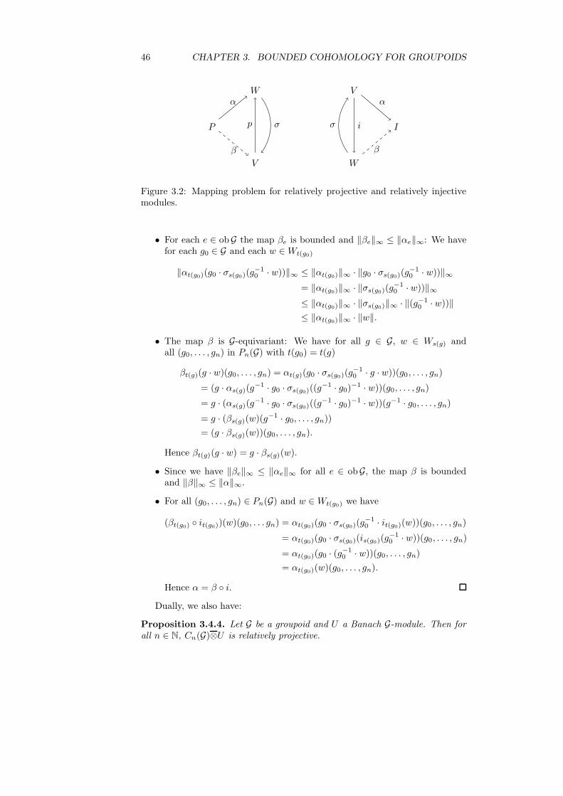
46 CHAPTER 3. BOUNDED COHOMOLOGY FOR GROUPOIDS
W
P
V
σp
α
β
V
I
W
σ i
α
β
Figure 3.2: Mapping problem for relatively projective and relatively injectivemodules.
• For each e ∈ obG the map βe is bounded and ‖βe‖∞ ≤ ‖αe‖∞: We havefor each g0 ∈ G and each w ∈Wt(g0)
‖αt(g0)(g0 · σs(g0)(g−10 · w))‖∞ ≤ ‖αt(g0)‖∞ · ‖g0 · σs(g0)(g
−10 · w))‖∞
= ‖αt(g0)‖∞ · ‖σs(g0)(g−10 · w))‖∞
≤ ‖αt(g0)‖∞ · ‖σs(g0)‖∞ · ‖(g−10 · w))‖
≤ ‖αt(g0)‖∞ · ‖w‖.
• The map β is G-equivariant: We have for all g ∈ G, w ∈ Ws(g) andall (g0, . . . , gn) in Pn(G) with t(g0) = t(g)
βt(g)(g · w)(g0, . . . , gn) = αt(g)(g0 · σs(g0)(g−10 · g · w))(g0, . . . , gn)
= (g · αs(g)(g−1 · g0 · σs(g0)((g
−1 · g0)−1 · w))(g0, . . . , gn)
= g · (αs(g)(g−1 · g0 · σs(g0)((g
−1 · g0)−1 · w))(g−1 · g0, . . . , gn)
= g · (βs(g)(w)(g−1 · g0, . . . , gn))
= (g · βs(g)(w))(g0, . . . , gn).
Hence βt(g)(g · w) = g · βs(g)(w).
• Since we have ‖βe‖∞ ≤ ‖αe‖∞ for all e ∈ obG, the map β is boundedand ‖β‖∞ ≤ ‖α‖∞.
• For all (g0, . . . , gn) ∈ Pn(G) and w ∈ Wt(g0) we have
(βt(g0) ◦ it(g0))(w)(g0, . . . gn) = αt(g0)(g0 · σs(g0)(g−10 · it(g0)(w))(g0, . . . , gn)
= αt(g0)(g0 · σs(g0)(is(g0)(g−10 · w))(g0, . . . , gn)
= αt(g0)(g0 · (g−10 · w))(g0, . . . , gn)
= αt(g0)(w)(g0, . . . , gn).
Hence α = β ◦ i.
Dually, we also have:
Proposition 3.4.4. Let G be a groupoid and U a Banach G-module. Then forall n ∈ N, Cn(G)⊗U is relatively projective.
3.4. RELATIVE HOMOLOGICAL ALGEBRA FOR GROUPOIDS 47
Proof. Let p : V −→ W be a relatively projective G-map between Banach G-modules and α : Cn(G)⊗U −→ W a G-map. Let σ : W −→ V be as in Defini-tion 3.4.2 (i). Define a G-map
β : Cn(G)⊗U −→ V
(g0, . . . , gn) ⊗ u 7−→ g0 · σ(α((ids(g0), g1, . . . , gn) ⊗ g−1
0 · u)).
A calculation similar to the one for the relative injective case shows that thismap indeed has the wanted properties.
Definition 3.4.5 (Strong Resolutions). Let (C∗, ∂∗) be a Banach G-chain com-plex, V a Banach G-module and ε : C0 −→ V a G-augmentation map. Wecall (C∗, ∂∗, ε) strong or a strong resolution for V if there exists a norm non-increasing chain contraction, i.e., a family
(sn : Cn −→ Cn+1)n∈N
s−1 : V −→ C0
of (not necessarily G-equivariant) R-morphisms between G-modules such that
(i) For all n ∈ N ∪ {−1} we have ‖sn‖∞ ≤ 1.
(ii) The family (sn)n∈N is a chain contraction of the augmented chain complex,i.e., for all n ∈ N>0
sn−1 ◦ ∂n + ∂n+1 ◦ sn = idCn,
and
s−1 ◦ ε + ∂1 ◦ s0 = idC0
ε ◦ s−1 = idV .
Dually, we also define strong resolutions for cochain complexes.
Example 3.4.6. Let G be a groupoid and V a Banach G-module. Recall fromRemark 3.2.20 the definition of the chain contraction s∗ : C∗(G) −→ C∗+1(G):
s−1 : R −→ C0(G)
e 7−→ ide
and for all n ∈ N
sn : Cn(G) −→ Cn+1(G)
(g0, . . . , gn) 7−→ (idt(g0), g0, . . . , gn).
(i) Consider the Banach G-chain complex C∗(G)⊗V together with the aug-mentation map
ε : Cℓ1
0 (G;V ) −→ V
g ⊗ v 7−→ v.
48 CHAPTER 3. BOUNDED COHOMOLOGY FOR GROUPOIDS
The family s∗ induces a norm-non increasing R-chain contraction sℓ1
∗
of (C∗(G)⊗V, ε) given by
sℓ1
∗ : Cℓ1
∗ (G;V ) −→ Cℓ1
∗+1(G;V )
x⊗ v 7−→ s∗(x) ⊗ v
and
sℓ1
−1 : V −→ Cℓ1
0 (G;V )
Ve ∋ v 7−→ ide⊗v.
In particular, (C∗(G)⊗V, ε) is a strong (homological) G-resolution of V .
(ii) Consider the Banach G-cochain complex B(C∗(G), V ) together with theaugmentation map ε : B(C0(G), V ) −→ V given by
ε : V −→ B(C0(G), V )
v 7−→ (g 7−→ v).
Then, the family s∗ induces a norm-non increasing R-cochain contrac-tion s∗b of (B(C∗(G), V ), ε) given by
s∗b : B(C∗(G), V ) −→ B(C∗−1(G), V )
ϕ 7−→ ϕ ◦ s∗
and setting for each e ∈ obG
s0b,e : B(C0(G)e, Ve) −→ Ve
ϕ 7−→ ϕ(ide).
In particular, (B(C∗(G), V ), ε) is a strong (cohomological) resolution of V .
Proposition 3.4.7 (Fundamental lemma I). Let (In, δnI )n∈N be a relatively in-jective Banach G-cochain complex and ε : W −→ I0 a G-augmentation map. Let((Cn, δnC)n∈N, ν : V −→ C0) be a strong G-resolution of a Banach G-module V .
Let f : V −→ W be a G-morphism. Then there exists an up to bounded G-cochain homotopy unique extension of f to a bounded G-cochain map betweenthe resolution (Cn, δnC , ν) and the augmented cochain complex (In, δnI , ε).
Proof. The proof is basically the same lifting argument as for all homological“fundamental lemmas”, for instance [62, Lemma 7.2.4].
Let ((sn : Cn −→ Cn−1)n∈N>0 , s0 : C0 −→ V ) be a norm non-increasing
cochain contraction of the augmented cochain complex. We construct the se-quence (fn)n∈N by induction.
The augmentation map ε : V −→ C0 is relatively injective (s0 ◦ ε = idV ).For this reason, because I0 is relatively injective, there exists a bounded G-lift f0 : C0 −→ I0 of ν ◦ f such that f0 ◦ ε = ν ◦ f .
C0 I0
V Wf
ν
f0
s0ε
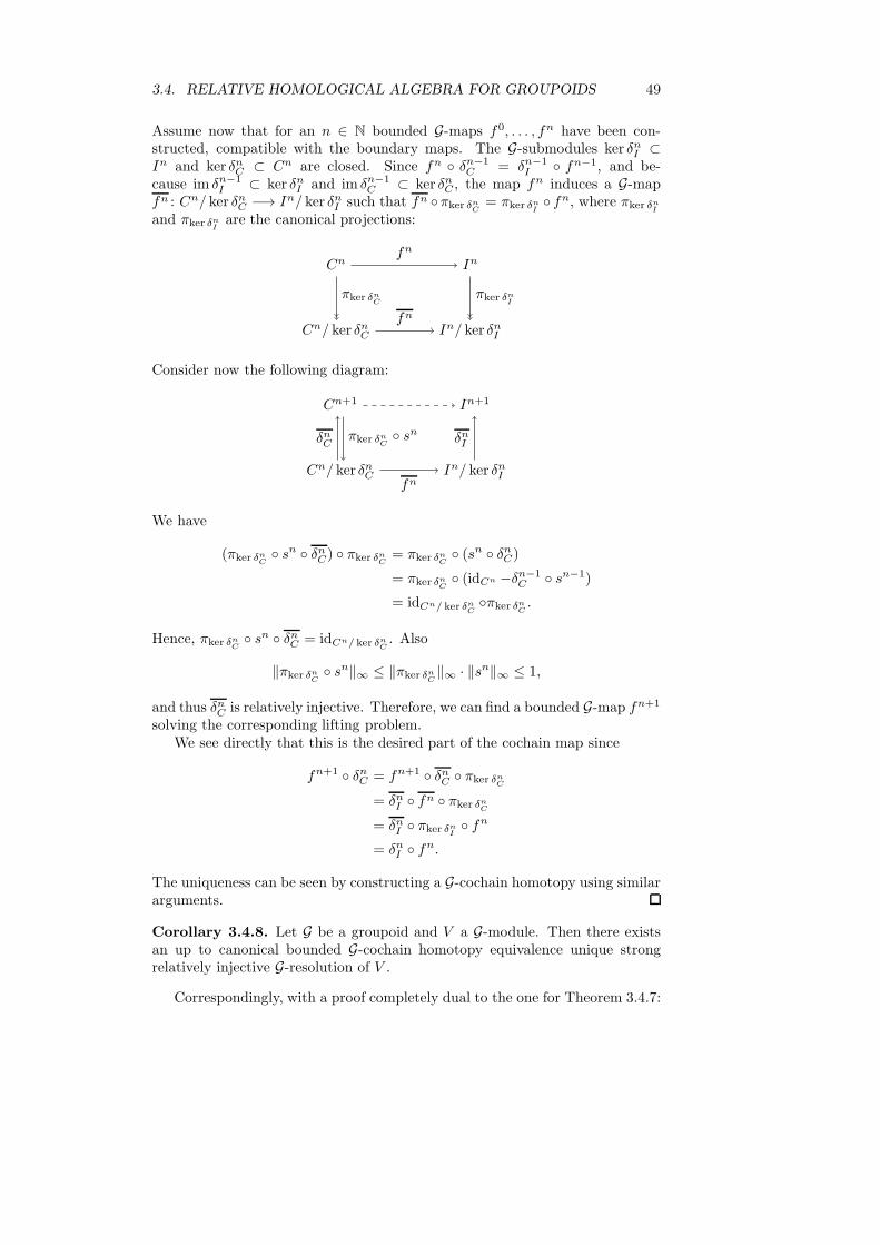
3.4. RELATIVE HOMOLOGICAL ALGEBRA FOR GROUPOIDS 49
Assume now that for an n ∈ N bounded G-maps f0, . . . , fn have been con-structed, compatible with the boundary maps. The G-submodules ker δnI ⊂In and ker δnC ⊂ Cn are closed. Since fn ◦ δn−1
C = δn−1I ◦ fn−1, and be-
cause im δn−1I ⊂ ker δnI and im δn−1
C ⊂ ker δnC , the map fn induces a G-mapfn : Cn/ ker δnC −→ In/ ker δnI such that fn ◦πker δn
C= πker δn
I◦ fn, where πker δn
I
and πker δnI
are the canonical projections:
Cn In
Cn/ ker δnC In/ ker δnIfn
πker δnC
πker δnI
fn
Consider now the following diagram:
Cn+1 In+1
Cn/ ker δnC In/ ker δnIfn
δnIπker δnC◦ snδnC
We have
(πker δnC◦ sn ◦ δnC) ◦ πker δn
C= πker δn
C◦ (sn ◦ δnC)
= πker δnC◦ (idCn −δn−1
C ◦ sn−1)
= idCn/ ker δnC◦πker δn
C.
Hence, πker δnC◦ sn ◦ δnC = idCn/ ker δnC
. Also
‖πker δnC◦ sn‖∞ ≤ ‖πker δn
C‖∞ · ‖sn‖∞ ≤ 1,
and thus δnC is relatively injective. Therefore, we can find a bounded G-map fn+1
solving the corresponding lifting problem.We see directly that this is the desired part of the cochain map since
fn+1 ◦ δnC = fn+1 ◦ δnC ◦ πker δnC
= δnI ◦ fn ◦ πker δnC
= δnI ◦ πker δnI◦ fn
= δnI ◦ fn.
The uniqueness can be seen by constructing a G-cochain homotopy using similararguments.
Corollary 3.4.8. Let G be a groupoid and V a G-module. Then there existsan up to canonical bounded G-cochain homotopy equivalence unique strongrelatively injective G-resolution of V .
Correspondingly, with a proof completely dual to the one for Theorem 3.4.7:

50 CHAPTER 3. BOUNDED COHOMOLOGY FOR GROUPOIDS
Proposition 3.4.9 (Fundamental lemma II). Let G be a groupoid. Let (P∗, ∂P∗ )
be a relatively projective Banach G-cochain complex and ε : P0 −→ V a G-aug-mentation map. Let (C∗, ∂
C∗ , ν : C0 −→W ) be a strong G-resolution of a Banach
G-module W .Let f : V −→ W be a G-morphism. Then there exists an up to bounded G-
chain homotopy unique extension of f to a bounded G-chain map between theaugmented chain complex (P∗, ∂
P∗ , ε) and the resolution (C∗, ∂
C∗ , ν).
Theorem 3.4.10 (Bounded groupoid cohomology via relative homological al-gebra). Let G be a groupoid and V a Banach G-module. Let ((D∗, δ∗D), ε : V −→D0) be a strong G-resolution of V .
Then for each strong cochain contraction of (D∗, ε) there exists a canoni-cal norm non-increasing cochain map of this resolution to the standard resolu-tion (B(Cn(G), V ))n∈N of V extending idV .
Proof. The argument is similar to the proof of Proposition 3.4.3, see also [48,Lemma 3.2.2] for the group case.
Let ((sn : Dn −→ Dn−1)n∈N, s0 : D0 −→ V ) be a norm non-increasing
cochain contraction of the augmented cochain complex. We will define fami-lies (αn
e : Dne −→ B(Cn(G)e, Ve))e∈ob G by induction over n ∈ N ∪ {−1}. First,
we set α−1 = idV . Assume we have defined αn−1 for some n ∈ N. Then we setfor all (g0, . . . , gn) ∈ Pn(G) and all ϕ ∈ Dn
t(g0)
αnt(g0)
(ϕ)(g0, . . . , gn) = αn−1t(g0)
(g0 · sns(g0)
(g−10 · ϕ))(g0 · g1, . . . , gn).
We immediately see that this is a G-map for all n ∈ N and since sn is norm non-increasing and the G-action is isometric, αn is norm non-increasing by induction.By a short calculation we see that (αn)n∈N is a cochain map.
Corollary 3.4.11. Let G be a groupoid and V a Banach G-module. Fur-thermore, let ((Dn, δnD)n∈N, ε : V −→ D0) be a strong relatively injective G-resolution of V . Then there exists a canonical semi-norm non-increasing iso-morphism of graded R-modules
H∗(D∗G) −→ H∗b (G;V ).
Proof. By Theorem 3.4.10 there exists a norm non-increasing G-cochain map
Dn −→ B(Cn(G), V ).
extending idV . This induces a norm non-increasing morphism
H∗(D∗G) −→ H∗b (G;V ).
By the fundamental lemma for groupoids, this is an isomorphism.
Dually, we get the following result for ℓ1-homology:
Theorem 3.4.12 (ℓ1-homology via relative homological algebra). Let G bea groupoid and V a G-module. Let ((E∗, ∂
E∗ ), ε : E0 −→ V ) be a strong G-
resolution of V .Then for each strong chain contraction of (E∗, ε) there exists a canonical
norm non-increasing chain map from the standard resolution (C∗(G)⊗V ) of Vto (E∗, ε) extending idV .

3.5. BOUNDED COHOMOLOGY FOR PAIRS OF GROUPOIDS 51
Proof. The proof is similar to the proof of Theorem 3.4.10:Let ((sn : En −→ En+1)n∈N, s−1 : V −→ E0) be a norm non-increasing chain
contraction of the augmented chain complex. By induction over n ∈ N ∪ {−1},we define a bounded G-chain map (αn : Cn(G)⊗V −→ En)n∈N. First, weset α−1 = idV . Assume we have defined αn−1 for some n ∈ N∪ {−1}. Then weset for all (g0, . . . , gn) ∈ Pn(G) and all v ∈ Vt(g0)
αn((g0, . . . , gn) ⊗ v) = g0 · sn−1(αn−1((g1, . . . , gn) ⊗ g−10 · v)).
We immediately see that this is a G-map for all n ∈ N and since sn−1 is normnon-increasing and the G-action is isometric, αn is norm non-increasing by in-duction. By a short calculation we see that (αn)n∈N is a chain map extendingidV .
Corollary 3.4.13. Let G be a groupoid and V a Banach G-module. Further-more, let ((E∗, ∂
E∗ ), ε : E0 −→ V ) be a strong relatively projective G-resolution
of V . Then there exists a canonical semi-norm non-increasing isomorphism ofgraded R-modules
Hℓ1
∗ (G;V ) −→ H∗(E∗G).
Proof. As for Corollary 3.4.11.
3.5 Bounded Cohomology for Pairs of Groupoids
3.5.1 Relative Bounded Cohomology
We will now define relative bounded cohomology for pairs of groupoids. Usingthis definition, we derive a long exact sequence for bounded cohomology ofgroupoids. Then, we show that relative bounded cohomology is a homotopyinvariant. Finally, we discuss the special case of a group relative to a familyof subgroups and get a long exact sequence relating bounded cohomology of agroup relative to a finite family of subgroups to the regular bounded homologyof the group and the subgroups. As before, we will also discuss relative ℓ1-homology where analogous results hold.
Though we do not elaborate relative (co-)homology for groupoid pairs, thedefinitions and results here can easily be adapted to the non-normed situation.
Definition 3.5.1. Let i : A −→ G be a groupoid pair, i.e. the canonical inclu-sion of a subgroupoid A ⊂ G. Let V be a G-module.
(i) The map
C∗(i;V ) : C∗(A; i∗V ) −→ C∗(G;V )
a⊗ v 7−→ a⊗ v
is injective and induces an injection Cℓ1
∗ (A; i∗V ) −→ Cℓ1
∗ (G;V ). Thequotient induced by this map
Cℓ1
∗ (G,A;V ) := Cℓ1
∗ (G;V )/Cℓ1
∗ (A; i∗V ),
endowed with the induced norm on the quotient, is a normed R-chain
complex. We write p(G,A;V )∗ : Cℓ1
∗ (G;V ) −→ Cℓ1
∗ (G,A;V ) for the canonicalprojection.

52 CHAPTER 3. BOUNDED COHOMOLOGY FOR GROUPOIDS
(ii) We call
Hℓ1
∗ (G,A;V ) := H∗(Cℓ1
∗ (G,A;V ))
the ℓ1-homology of G relative A with coefficients in V .
(iii) Dually, the map
C∗b (i;V ) : C∗
b (G;V ) −→ C∗b (A, i∗V )
(fe)e∈obG 7−→ (fe|C∗(A)e)e∈obA
is surjective. Its kernel
C∗b (G,A;V ) := ker(C∗
b (i;V ))
={f ∈ BG(C∗(G), V ) | ∀e∈obA fe|C∗(A)e = 0},
endowed with the induced norm on the subspace, is a normed R-cochaincomplex. We write ι∗(G,A;V ) : C∗
b (G,A;V ) −→ C∗b (G;V ) for the canoncial
inclusion.
(iv) We callH∗
b (G,A;V ) := H∗(C∗b (G,A;V ))
the bounded cohomology of G relative to A with coefficients in V .
We define domain categories Grp2Ban and Grp2Ban analogously to the def-inition of GrpBan and GrpBan by considering pairs of groupoids instead ofgroupoids.
Definition 3.5.2.
(i) Let (f, ϕ) : ((G,A), V ) −→ ((H,B),W ) be a morphism in Grp2Ban. ThenC∗(f ;ϕ) induces a bounded chain map
Cℓ1
∗ (f, f |A;ϕ) : Cℓ1
∗ (G,A;V ) −→ Cℓ1
∗ (H,B;W );
and a continuous map between graded normed modules
Hℓ1
∗ (f, f |A;ϕ) : Hℓ1
∗ (G,A;V ) −→ Hℓ1
∗ (H,B;W ).
This defines a functor Grp2Ban −→ R-Mod‖·‖∗ .
(ii) Let (f, ϕ) : ((G,A), V ) −→ ((H,B),W ) be a morphism in Grp2Ban. ThenC∗
b (f, ϕ) restricts to a bounded cochain map
C∗b (f, f |A;ϕ) := C∗
b (f ;ϕ)|C∗b(H,B;W ) : C∗
b (H,B;W ) −→ C∗b (G,A;V ).
This induces a continuous map between graded normed modules
H∗b (f, f |A;ϕ) : H∗
b (H,B;W ) −→ H∗b (G,A;V ).
This defines a contravariant functor Grp2Ban −→ R-Mod‖·‖∗ .
As for the above definition, we just note that the right-hand square in thefollowing diagram commutes by definition, so the map on the left-hand side isdefined:

3.5. BOUNDED COHOMOLOGY FOR PAIRS OF GROUPOIDS 53
0 C∗b (H,B;W ) C∗
b (H;W ) C∗b (B; i∗BW ) 0
0 C∗b (G,A;V ) C∗
b (G;V ) C∗b (A; i∗AV ) 0
ι∗(H,B;W )
ι∗(G,A;V )
C∗b (f, f |A;ϕ)
C∗b (iB;V )
C∗b (f ;ϕ)
C∗b (iA;V )
C∗b (f |A; i∗Aϕ)
Here i∗Aϕ : f |∗Ai∗BW = i∗Af
∗V −→ i∗AV denotes the A-map given by (ϕa)a∈obG ,i.e., by restricting the family corresponding to ϕ to objects in A. Functorialitythen follows from the functoriality of the right-hand square. Similarly for ℓ1-homology.
In particular, we can apply the snake lemma to get the following:
Proposition 3.5.3. Let iA : A −→ G be the inclusion of a subgroupoid .
(i) There is a natural (with respect to morphisms in Grp2Ban) long exactsequence
· · · Hℓ1
∗ (A; i∗AV ) Hℓ1
∗ (G;V ) Hℓ1
∗ (G,A;V ) Hℓ1
∗−1(A; i∗AV ) · · ·Hℓ1
∗ (iA;V ) H∗(p(G,A;V )∗ ) ∂∗
such that ∂∗ is continuous with respect to the induced semi-norms.
(ii) There is a natural (with respect to morphisms in Grp2Ban) long exactsequence
· · · H∗b (G,A;V ) H∗
b (G;V ) H∗b (A; i∗AV ) H∗+1
b (G,A;V ) · · ·
H∗(ι∗(G,A;V )) H∗b (iA;V ) δ∗
such that δ∗ is continuous with respect to the induced semi-norms.
Definition 3.5.4. Let f, g : (G,A) −→ (H,B) be maps of pairs of groupoids.We call a homotopy h between f and g a homotopy relative A if for all a ∈ Athe morphism Ha : f(a) −→ g(a) is contained in B.
In this situation, we also write f ≃A,B g. The restriction of h induces thena homotopy h|A between f |A, g|A : A −→ B.
We can give an equivalent description of relative homotopies using Proposi-tion 3.1.9:
Remark 3.5.5. Let f, g : (G,A) −→ (H,B) be maps of pairs of groupoids and ha homotopy between f and g. Let H : G × ∆1 −→ H be the induced groupoidmap, as in Proposition 3.1.9. Then h is a homotopy relative A if and only if Hrestricts to a groupoid map A× ∆1 −→ B.
Proposition 3.5.6.
(i) Let f, g : (G,A) −→ (H,B) be maps of pairs of groupoids and V be an H-module. If f ≃A,B g via a homotopy h, then there is a canonical R-cochainhomotopy between C∗
b (f, f |A;V ) and C∗b (g, g|A;V ◦ h).

54 CHAPTER 3. BOUNDED COHOMOLOGY FOR GROUPOIDS
(ii) In particular,
H∗b (f, f |A;V ) = H∗
b (idG , idA;V ◦ h) ◦H∗b (g, g|A;V );
and the map H∗b (idG , idA;V ◦ h) is an isometric isomorphism.
Proof.
(i) We write sh∗ and sh|A∗ for the G-chain homotopies constructed in Proposi-
tion 3.2.30 (i) with respect to h and h|A. Let s∗V,h and s∗i∗BV,h|Adenote the
cochain homotopies induced by sh∗ and sh|A∗ . The right-hand side square
of the following diagram
0 C∗b (H,B;V ) C∗
b (H;V ) C∗b (B; i∗BV ) 0
0 C∗−1b (G,A; f∗V ) C∗−1
b (G; f∗V ) C∗−1b (A; i∗Af
∗V ) 0.
ι∗(H,B;V )
ι∗−1(G,A;f∗V )
s∗V,h|C∗(H,B;V )
C∗b (iB;V )
s∗i∗BV,h|A
C∗−1b (iA; f∗V )
s∗V,h
commutes by definition, since for all (ψe)e∈obH ∈ C∗b (H;V )
(C∗−1b (ia;V ) ◦ s∗V,h)(ψe)e∈H = (ψf(e) ◦ s
h∗,e)e∈obA
= (ψf |A(e) ◦ sh|A∗,e )e∈obA
= s∗i∗BV,h|A(ψe)e∈obB
= (s∗i∗BV,h|A◦ C∗
b (iB;V ))(ψe)e∈obH.
Hence the map on the left-hand side is defined. The map s∗i∗BV,h|Ais a
cochain homotopy between
C∗b (f |A, i
∗BV ) = C∗
b (f |A, idf |∗Ai∗BV )
= C∗b (f |A, idi∗Af∗V )
= C∗b (f |A, i
∗A idf∗V )
and
C∗b (g|A, (V ◦ h|A)) = C∗
b (g|A, i∗A(V ◦ h)).
Hence, by comparing the diagrams defining C∗b (f, f |A;V ), C∗
b (g, g|A;V )and s∗V,h|C∗(H,B;V ), we see that s∗V,h|C∗(H,B;V ) defines an R-cochain homo-topy between C∗
b (f, f |A;V ) and C∗b (g, g|A;V ).
(ii) The map C∗b (idG , idA;V ◦ h) is an isometric cochain isomorphism, since
C∗b (idG ;V ◦h) and C∗
b (idA; i∗A(V ◦h)) = C∗b (idA; i∗AV ◦h|A)) are isometric
cochain isomorphisms.
Corollary 3.5.7. Let f : (G,A) −→ (H,B) be an equivalence relative A, i.e.,there exists a map g : (H,B) −→ (G,A), such that g ◦f ≃A,B idG and f ◦g ≃B,A
idH. ThenH∗
b (f, f |A;V ) : H∗b (H,B;V ) −→ H∗
b (G,A; f∗V )
is an isometric isomorphism.
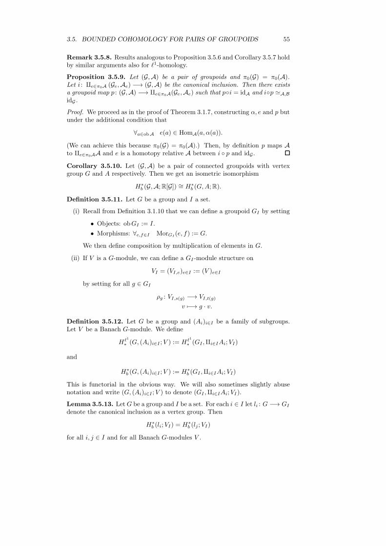
3.5. BOUNDED COHOMOLOGY FOR PAIRS OF GROUPOIDS 55
Remark 3.5.8. Results analogous to Proposition 3.5.6 and Corollary 3.5.7 holdby similar arguments also for ℓ1-homology.
Proposition 3.5.9. Let (G,A) be a pair of groupoids and π0(G) = π0(A).Let i : ∐e∈π0A (Ge,Ae) −→ (G,A) be the canonical inclusion. Then there existsa groupoid map p : (G,A) −→ ∐e∈π0A(Ge,Ae) such that p◦i = idA and i◦p ≃A,B
idG .
Proof. We proceed as in the proof of Theorem 3.1.7, constructing α, e and p butunder the additional condition that
∀a∈obA e(a) ∈ HomA(a, α(a)).
(We can achieve this because π0(G) = π0(A).) Then, by definition p maps Ato ∐e∈π0AA and e is a homotopy relative A between i ◦ p and idG .
Corollary 3.5.10. Let (G,A) be a pair of connected groupoids with vertexgroup G and A respectively. Then we get an isometric isomorphism
H∗b (G,A;R[G]) ∼= H∗
b (G,A;R).
Definition 3.5.11. Let G be a group and I a set.
(i) Recall from Definition 3.1.10 that we can define a groupoid GI by setting
• Objects: obGI := I.
• Morphisms: ∀e,f∈I MorGI(e, f) := G.
We then define composition by multiplication of elements in G.
(ii) If V is a G-module, we can define a GI -module structure on
VI = (VI,e)e∈I := (V )e∈I
by setting for all g ∈ GI
ρg : VI,s(g) −→ VI,t(g)
v 7−→ g · v.
Definition 3.5.12. Let G be a group and (Ai)i∈I be a family of subgroups.Let V be a Banach G-module. We define
Hℓ1
∗ (G, (Ai)i∈I ;V ) := Hℓ1
∗ (GI ,∐i∈IAi;VI)
and
H∗b (G, (Ai)i∈I ;V ) := H∗
b (GI ,∐i∈IAi;VI)
This is functorial in the obvious way. We will also sometimes slightly abusenotation and write (G, (Ai)i∈I ;V ) to denote (GI ,∐i∈IAi;VI).
Lemma 3.5.13. LetG be a group and I be a set. For each i ∈ I let li : G −→ GI
denote the canonical inclusion as a vertex group. Then
H∗b (li;VI) = H∗
b (lj ;VI)
for all i, j ∈ I and for all Banach G-modules V .

56 CHAPTER 3. BOUNDED COHOMOLOGY FOR GROUPOIDS
Proof. We can define a homotopy between li and lj by setting
h1 := idG : G = Gi −→ Gj = G.
Here 1 denotes the unique vertex of G. Hence, by Proposition 3.3.14
H∗b (li;VI) = H∗
b (idG;VI ◦ h) ◦H∗b (lj ;VI) = H∗
b (lj ;VI).
Theorem 3.5.14. Let G be a group and (Ai)i∈I a finite family of subgroups.Let V be a Banach G-module. Then there is a natural long exact sequence
· · · H∗b (G, (Ai)i∈I ;V ) H∗
b (G;V )∏
i∈I H∗b (Ai; i
∗AiV ) H∗+1
b (G, (Ai)i∈I ;V ) · · ·ι∗ (H∗
b (iAi;V ))i∈I d∗
such that δ∗ is continuous with respect to the induced semi-norm and the productsemi-norm. Here
ι∗ := H∗b (le;VI) ◦H∗(ιGI ,AI ,VI
).
where le : G −→ GI is the canonical inclusions for some vertex e ∈ obG.
Proof. Write tj : Aj −→ ∐i∈IAi and s : ∐i∈I Ai −→ GI for the canonicalinclusions. By Corollary 3.1.8 and Proposition 3.3.18, the rows in the followingdiagram are isometric isomorphisms:
......
H∗b (G; (Ai)i∈I ;V ) H∗
b (G; (Ai)i∈I ;V )
H∗b (GI ;VI) H∗
b (G;V )
H∗b (∐i∈IAi; s
∗V )∏
i∈I H∗b (Ai; i
∗AiV )
H∗+1b (G, (Ai)i∈I ;V ) H∗+1
b (G, (Ai)i∈I ;V )
......
=
H∗b (le;VI)
∼=
(H∗b (ti; s
∗V ))i∈I
∼=
=
H∗(ι∗(G,(Ai)i∈I ;V ))
H∗b (s;VI)
δ∗
ι∗
(H∗b (iAi
;V ))i∈I
d∗
The upper square commutes by definition and we can choose a continuousmap d∗ in such a way, that the lower square commutes. The centre squarecommutes by Lemma 3.5.13.
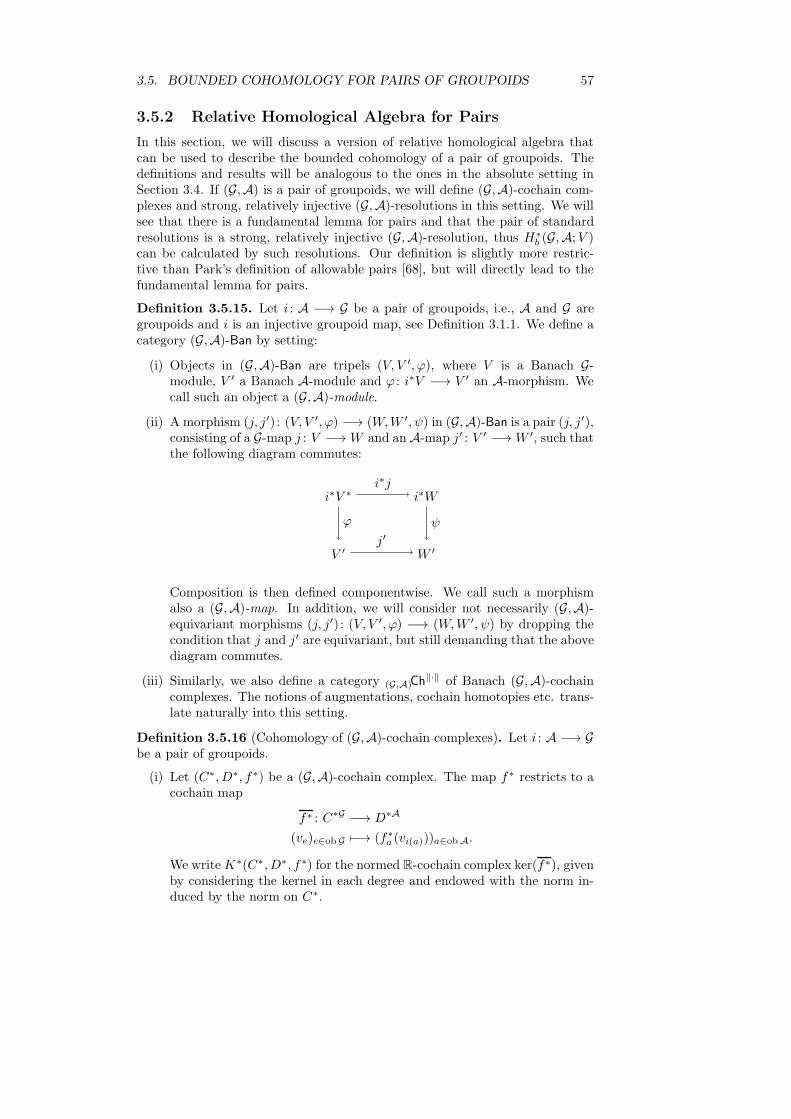
3.5. BOUNDED COHOMOLOGY FOR PAIRS OF GROUPOIDS 57
3.5.2 Relative Homological Algebra for Pairs
In this section, we will discuss a version of relative homological algebra thatcan be used to describe the bounded cohomology of a pair of groupoids. Thedefinitions and results will be analogous to the ones in the absolute setting inSection 3.4. If (G,A) is a pair of groupoids, we will define (G,A)-cochain com-plexes and strong, relatively injective (G,A)-resolutions in this setting. We willsee that there is a fundamental lemma for pairs and that the pair of standardresolutions is a strong, relatively injective (G,A)-resolution, thus H∗
b (G,A;V )can be calculated by such resolutions. Our definition is slightly more restric-tive than Park’s definition of allowable pairs [68], but will directly lead to thefundamental lemma for pairs.
Definition 3.5.15. Let i : A −→ G be a pair of groupoids, i.e., A and G aregroupoids and i is an injective groupoid map, see Definition 3.1.1. We define acategory (G,A)-Ban by setting:
(i) Objects in (G,A)-Ban are tripels (V, V ′, ϕ), where V is a Banach G-module, V ′ a Banach A-module and ϕ : i∗V −→ V ′ an A-morphism. Wecall such an object a (G,A)-module.
(ii) A morphism (j, j′) : (V, V ′, ϕ) −→ (W,W ′, ψ) in (G,A)-Ban is a pair (j, j′),consisting of a G-map j : V −→W and an A-map j′ : V ′ −→W ′, such thatthe following diagram commutes:
i∗V ∗ i∗W
V ′ W ′
i∗j
ϕ
j′ψ
Composition is then defined componentwise. We call such a morphismalso a (G,A)-map. In addition, we will consider not necessarily (G,A)-equivariant morphisms (j, j′) : (V, V ′, ϕ) −→ (W,W ′, ψ) by dropping thecondition that j and j′ are equivariant, but still demanding that the abovediagram commutes.
(iii) Similarly, we also define a category (G,A)Ch‖·‖ of Banach (G,A)-cochain
complexes. The notions of augmentations, cochain homotopies etc. trans-late naturally into this setting.
Definition 3.5.16 (Cohomology of (G,A)-cochain complexes). Let i : A −→ Gbe a pair of groupoids.
(i) Let (C∗, D∗, f∗) be a (G,A)-cochain complex. The map f∗ restricts to acochain map
f∗ : C∗G −→ D∗A
(ve)e∈ob G 7−→ (f∗a (vi(a)))a∈obA.
We write K∗(C∗, D∗, f∗) for the normed R-cochain complex ker(f∗), givenby considering the kernel in each degree and endowed with the norm in-duced by the norm on C∗.

58 CHAPTER 3. BOUNDED COHOMOLOGY FOR GROUPOIDS
(ii) Let (j, j′) : (C∗0 , D
∗0 , f
∗0 ) −→ (C∗
1 , D∗1 , f
∗1 ) be a (G,A)-cochain map. Then,
by restriction, (j, j′) induce the maps on the right-hand side of the follow-ing diagram
ker f∗0 C∗G
0 D∗A0
ker f∗1 C∗G
1 D∗A1 ,
j∗|ker f∗0
j∗
f∗0
f∗1
j′∗
and this square commutes, hence the map on left-hand side is defined.We write K∗(j, j′) := j∗|ker f∗
0for the map on the left-hand side. In this
way, K∗ defines a functor (G,A)Ch‖·‖ −→ RCh
‖·‖.
(iii) We write H∗(C∗, D∗, f∗) to denote the cohomology of K∗(C∗, D∗, f∗)endowed with the induced semi-norm. In this way, we have defined a
functor (G,A)Ch‖·‖ −→ R-Mod
‖·‖∗ .
The main example of (G,A)-cochain complexes in this section is given bythe pair of canonical resolutions for G and A:
Example 3.5.17. Let i : A −→ G be a groupoid pair and V a Banach G-module. Then C∗(G,A;V ) := (B(C∗(G), V ), B(C∗(A), i∗V ), B(C∗(i), V )) is aBanach (G,A)-cochain complex. By definition
H∗(C∗(G,A;V )) = H∗b (G,A;V ).
Remark 3.5.18. Let (f∗0 , f
∗1 ), (g∗0 , g
∗1) : (C∗
0 , C∗1 , ϕ
∗) −→ (D∗0 , D
∗1 , ψ
∗) be a pairof (G,A)-cochain maps. Let (h∗0, h
∗1) : (C∗
0 , C∗1 , ϕ
∗0) −→ (D∗−1
0 , D∗−11 , ψ∗−1) be
a (G,A)-cochain homotopy between (f∗0 , f
∗1 ) and (g∗0 , g
∗1), i.e., h∗0 is a G-cochain
homotopy between f∗0 and g∗0 and h∗1 is an A-cochain homotopy between f∗
1
and g∗1 , and the pair (h∗0, h∗1) is a family of (G,A)-maps. Then (h∗0, h
∗1) induces
an R-cochain homotopy between K∗(f∗0 , f
∗1 ) and K∗(g∗0 , g
∗1). In this sense, co-
homology of (G,A)-cochain complexes is a homotopy invariant.
Definition 3.5.19 (Relatively injective pairs). Let i : A −→ G be a pair ofgroupoids.
(i) A (G,A)-map (j, j′) : (V, V ′, ϕ) −→ (W,W ′, ψ) is called relatively injective,if there is a (not necessarily (G,A)-equivariant) split
(σ, σ′) : (W,W ′, ψ) −→ (V, V ′, ϕ),
such that (σ, σ′) ◦ (j, j′) = (idV , idV ′) and ‖σ‖∞ ≤ 1 and ‖σ′‖∞ ≤ 1.
(ii) A (G,A)-module (I, I ′, f) is called relatively injective if for each relativelyinjective (G,A)-map (j, j′) : (V, V ′, ϕ) −→ (W,W ′, ψ) between (G,A)-mo-dules and each (G,A)-map (α, α′) : (V, V ′, ϕ) −→ (I, I ′, f), there existsa (G,A)-map (β, β′) : (W,W ′, ψ) −→ (I, I ′, f), such that (β, β′) ◦ (j, j′) =(α, α′) and ‖β‖∞ ≤ ‖α‖∞ and ‖β′‖∞ ≤ ‖α′‖∞.

3.5. BOUNDED COHOMOLOGY FOR PAIRS OF GROUPOIDS 59
i∗V V ′
i∗I I ′
i∗W W ′
i∗σ
i∗j
i∗α
ϕ
ψ
f
j′
σ′ α′
i∗ββ′
Figure 3.3: Extension Problem for Pairs.
Remark 3.5.20. Park [68] treats bounded cohomology of a pair (G,A) ofgroups via so called allowable resolutions, i.e., via pairs consisting of a strong,relatively injective G-resolution and a strong, relatively injective A-resolution,together with a cochain map that commutes with a pair of norm non-increasingcochain contractions of the two resolutions. Thus, the condition on relativelyinjectivity of an allowable pair is a priori weaker than our definition of relativelyinjective (G,A)-resolutions. However, as noted by Frigerio and Pagliantini [40,Remark 3.8], it is not clear why Park’s definition should lead to a version of thefundamental lemma. Our definition avoids this problem and still includes theinteresting examples.
Example 3.5.21. Let i : A −→ G be a pair of groupoids and U a Banach G-module. For each n ∈ N, the Banach (G,A)-module Cn(G,A;U) is relativelyinjective.
Proof. Let (j, j′) : (V, V ′, ϕ) −→ (W,W ′, ψ) be a relatively injective (G,A)-mapand let (σ, σ′) : (W,W ′, ψ) −→ (V, V ′, ϕ) be a not necessarily equivariant splitfor (j, j′) with ‖σ‖∞ ≤ 1 and ‖σ′‖∞ ≤ 1. Moreover, let (α, α′) : (V, V ′, ϕ) −→Cn(G,A;U) be a (G,A)-map. As in the proof of Proposition 3.4.3, we definea G-map β : W −→ B(Cn(G), U) and an A-map β′ : W ′ −→ B(Cn(A), i∗U) bysetting
β : W −→ B(Cn(G), U)
w 7−→(
(g0, . . . , gn) 7−→ α(g0 · σ(g−10 · w))(g0, . . . , gn)
)
and
β′ : W −→ B(Cn(A), i∗U)
w 7−→(
(a0, . . . , an) 7−→ α′(a0 · σ′(a−1
0 · w))(a0, . . . , an)).
In particular, (β, β′) ◦ (j, j′) = (α, α′) and ‖β‖∞ ≤ ‖α‖∞ and ‖β′‖∞ ≤ ‖α′‖∞.

60 CHAPTER 3. BOUNDED COHOMOLOGY FOR GROUPOIDS
We have for all w ∈ i∗W and (a0, . . . , a0) ∈ Cn(A)
β′(ψ(w))(a0, . . . , an) = α′(a0 · σ′(a−1
0 · ψ(w)))(a0, . . . , an)
= α′(a0 · ϕi∗σ(a−1
0 · w))(a0, . . . , an)
= B(Cn(i), U)i∗α(a0 · i∗σ(a−1
0 · w))(a0, . . . , an)
= B(Cn(i), U)i∗β(w)(a0, . . . , an).
Hence, (β, β′) is a (G,A)-map.
Definition 3.5.22. Let i : A −→ G be a pair of groupoids, (C∗, D∗, f∗) be aBanach (G,A)-cochain complex and V be a Banach G-module. Furthermore,let (ε, ε′) : (V, i∗V, idi∗V ) −→ (C0, D0, f0) be a (G,A)-augmentation map. Wecall (C∗, D∗, f∗, (ε, ε′)) a strong resolution of V if there exists a (not neces-sarily (G,A)-equivariant) norm non-increasing cochain contraction (s∗, t∗) of(C∗, D∗, f∗, (ε, ε′)), i.e., a norm non-increasing contraction s∗ of (C∗, ε) and anorm non-increasing contraction t∗ of (D∗, ε′), such that f∗ commutes with i∗s∗
and t∗.
Let i : A −→ G be a groupoid pair and V a G-module. Recall that there isa G-augmentation map
ε : V −→ B(C0(G), V )
v 7−→ (g 7−→ v)
and an A-augmentation map
ε′ : i∗V −→ B(C0(A), i∗V )
v 7−→ (a 7−→ v).
This induces a canonical (G,A)-augmentation map
(ε, ε′) : (V, i∗V, idi∗V ) −→ C0(G,A;V ).
Example 3.5.23. Let i : A −→ G be a pair of groupoids and V be a Ba-nach G-module. Let s∗G and s∗A be the norm-non-increasing cochain contrac-tions for (B(C∗(G), V ), ε) and (B(C∗(A), i∗V ), ε′) as in Example 3.4.6. By ashort calculation, we see that (s∗G , s
∗A) is a norm non-increasing cochain con-
traction of (C∗(G,A;V ), (ε, ε′)). Hence, (C∗(G,A;V ), (ε, ε′)) is a strong (G,A)-resolution of V , called the standard (G,A)-resolution of V .
Proposition 3.5.24 (Fundamental Lemma for Pairs). Let i : A −→ G be apair of groupoids. Let (I∗, J∗, ϕ∗) be a relatively injective (G,A)-cochain com-plex and (ε, ε′) : (W, i∗W, idi∗W ) −→ (I0, J0, ϕ0) a (G,A)-augmentation map.Let (C∗, D∗, ψ∗, (ν, ν′)) be a strong (G,A)-resolution of a Banach G-module V .Let (f, f ′) : (V, i∗V, idi∗V ) −→ (W, i∗W, idi∗W ) be a (G,A)-map. Then thereexists an extension of (f, f ′) to a bounded (G,A)-cochain map from the resolu-tion (C∗, D∗, ψ∗, (ν, ν′)) to the augmented cochain complex (I∗, J∗, ϕ∗, (ε, ε′)).This extension is unique up to bounded (G,A)-cochain homotopy.
Proof. The proof is the same as the one of Proposition 3.4.7, just solving theextension problems for pairs instead of for single modules.

3.5. BOUNDED COHOMOLOGY FOR PAIRS OF GROUPOIDS 61
Proposition 3.5.25. Let i : A −→ G be a groupoid pair and V a Banach G-module. Let (C∗, D∗, ϕ∗, (ν, ν′)) be a strong (G,A)-resolution of V . Then foreach norm non-increasing cochain contraction of (C∗, D∗, ϕ∗, (ν, ν′)) there existsa canonical, norm non-increasing (G,A)-cochain map
(C∗, D∗, ϕ∗) −→ C∗(G,A;V ),
extending (idV , idi∗V ).
Proof. The proof is basically the same as the one for Theorem 3.4.10, one justhas to check that the constructed pair of maps is a (G,A)-map.
Corollary 3.5.26. Let i : A −→ G be a groupoid pair and V a Banach G-module. Let (C∗, D∗, ϕ∗, (ν, ν′)) be a strong, relatively injective (G,A)-resolu-tion of V . Then there exists a canonical, semi-norm non-increasing isomorphismof graded R-modules
H∗(C∗, D∗, ϕ∗) −→ H∗b (G,A;V ).
Proof. By Proposition 3.5.25, there is a norm non-increasing (G,A)-cochain map
(C∗, D∗, ϕ∗) −→ C∗(G,A;V ),
extending (idV , idi∗V ). Therefore, this map induces a semi-norm non-increasingmap H∗(C∗, D∗, ϕ∗) −→ H∗
b (G,A;V ). By the fundamental lemma for pairs,this map is an isomorphism in each degree and does not depend of the choiceof the lift of (idV , idi∗V ).

62 CHAPTER 3. BOUNDED COHOMOLOGY FOR GROUPOIDS
Chapter 4
Amenable Groupoids andTransfer
Amenable groups are a major class of groups considered in geometric grouptheory and beyond. On the one hand, they include many interesting examples,e.g., all finite groups, all solvable groups and all groups of subexponential growthand are closed under taking extensions, subgroups, etc., [26]. On the other hand,their defining property, the existence of invariant means, makes them in manyinstances rather accessible.
The profound importance of amenable groups for the study of bounded co-homology comes from the fact that they are “invisible” to bounded cohomology,i.e., the bounded cohomology of amenable groups vanishes [65], see Section 4.2.This vanishing can in fact be used to completely describe amenable groupsvia bounded cohomology. That higher homotopy groups are Abelian and thusamenable will also be central in the proof of the (topological) mapping theorem,which can be expressed roughly as saying that the higher homotopy groups arenot seen by bounded cohomology, see Chapter 5.
Amenable groups will also be important in Chapter 6, where we will studytheir relation to uniformly finite homology.
The concept of amenability has been fruitfully extended to measured andtopological actions of groups. The action groupoid for such actions becomes ameasured or topological groupoid, leading to a further extension of amenabilityto such groupoids, [1, 2] for an overview of these concepts. However, since weare only considering discrete groupoids, we will give a definition of amenablegroupoids without additional structure that is sufficient for the latter applica-tions. Though it is beyond the scope of this thesis, it would be very interestingto modify the constructions of the previous sections to measured and topolog-ical groupoids in order to describe amenability in these settings via boundedcohomology.
This chapter is structured as follows. In the first section,we will presentour definition of amenable groupoids and give some examples. In the secondsection, we will show that bounded cohomology of amenable groupoids vanishesand that amenability can indeed be characterised by this vanishing. We will alsoprove the algebraic mapping theorem, stating that, in degree greater or equal 2,the bounded cohomology of a groupoid G relative to an amenable subgroupoid
63
64 CHAPTER 4. AMENABLE GROUPOIDS AND TRANSFER
is isometrically isomorphic to the bounded cohomology of G.
4.1 Amenability
In this section, we present our definition of amenability for groupoids, similarto the definition of amenability of measured groupoids, [1].
Definition 4.1.1. Let G be a groupoid and V a normed G-module. We definea normed G-module ℓ∞(G, V ) by:
(i) For all e ∈ obG we set ℓ∞(G, V )e := ℓ∞(Ge, Ve), endowed with the ‖ · ‖∞-norm. Here, we denote by Ge the set of all morphisms in G ending in e,i.e., Ge = t−1(e).
(ii) We define the partial G-action by setting for all g ∈ G
ρg : ℓ∞(G, V )s(g) −→ ℓ∞(G, V )t(g)
ϕ 7−→(h 7−→ g · ϕ(g−1 · h)).
Remark 4.1.2. If G is a groupoid and V a normed G-module, there is a canon-ical G-inclusion map cV : V −→ ℓ∞(G, V ), corresponding to viewing elementsin V as constant functions G −→ V , given by setting for all e ∈ obG
cV e : Ve −→ ℓ∞(G, V )e
a 7−→ (g 7−→ a).
Definition 4.1.3. Let G be a groupoid and V a normed G-module.
(i) An equivariant mean on G with coefficients in V is a G-morphism
m : ℓ∞(G, V ) −→ V,
satisfying ‖m‖∞ = 1 and m ◦ cV = idV .
If V = R[G], we call m simply a (left)-invariant mean on G.
(ii) We call G amenable if there exists a (left-)invariant mean on G.
This definition clearly extends the classical definition of amenability forgroups [69].
Example 4.1.4. Let (Ai)i∈I be a family of groups. Then ∐i∈IAi is amenableif and only if all Ai are amenable groups.
Example 4.1.5. Let G be an amenable group acting on a set X . Then theaction groupoid G⋉X is amenable (Example 3.1.5).
Proof. The canonical projection
π : G⋉X −→ G
(g, x) 7−→ g
is a groupoid map. Clearly π∗R ∼=G⋉X R[G⋉X ], and a short calculation showsthat π∗ℓ∞(G,R) ∼=G⋉X ℓ∞(G⋉X,R[G⋉X ]). Therefore, if m : ℓ∞(G,R) −→ R
is a left-invariant mean on G, the induced map π∗m is a left-invariant meanon G⋉X .
4.2. THE ALGEBRAIC MAPPING THEOREM 65
Proposition 4.1.6. Let G be an amenable groupoid and V a normed G-module.Then there exists an equivariant mean on G with coefficients in V ′
Proof. Let mR be a left-invariant mean on G. Then the map
mV : ℓ∞(G, V ′) −→ V ′
ϕ 7−→(v 7−→ mn
R
(g 7−→ ϕ(g)(v)
)).
is clearly an equivariant mean on G with coefficients in V ′.
4.2 The Algebraic Mapping Theorem
In this section, we show that the bounded cohomology of a groupoid G relativeto an amenable groupoid is equal to the bounded cohomology of G. We will alsoprove that the bounded cohomology of an amenable groupoid vanishes and thatthis characterises amenable groupoids. The techniques used are similar to thegroup case, [62, 65].
Let i : A −→ G be a pair of groupoids. Recall that we write L∗(G) to denotethe homogeneous Bar resolution of G, Definition 3.2.22. Let V be a Banach G-module. Denote by K∗
L(G,A;V ) the kernel of the map
B(L∗(i), V ) : B(L∗(G), V ) 7−→ B(L∗(A), i∗V ).
and write j∗ : K∗L(G,A;V ) −→ B(L∗(G), V ) to denote the canonical inclusion.
Since by Proposition 3.2.23 there is a natural and canonical isometric isomor-phism between L∗(G) and C∗(G), there is a canonical isometric isomorphismbetween K∗
L(G,A;V ) and K∗(G,A;V ). Thus we can also use the former tocalculate bounded cohomology of the pair (G,A).
Proposition 4.2.1. Let G be a groupoid. The following map is a norm non-increasing G-chain map extending idR[G]
Altn : Ln(G) −→ Ln(G)
(g0, . . . , gn) 7−→1
(n+ 1)!·∑
σ∈Σn+1
sgn(σ) · (gσ(0), . . . , gσ(n))
For a Banach G-module V , we write AltnV : B(Ln(G), V ) −→ B(Ln(G), V ) forthe corresponding dual map.
Proof. The only assertion that might want a proof is that Altn is a chain map.But for all e ∈ obG and (g0, . . . , gn) ∈ (Ge)
n+1
Altn−1∂n(g0, . . . , gn)
=
n∑
i=0
(−1)i ·1
n!·
∑
σ∈Σn+1,σ(i)=i
sgn(σ) · (gσ(0), . . . , gσ(i), . . . , gσ(n))
=
n∑
i=0
(−1)i ·1
(n+ 1)!·∑
σ∈Σn+1
sgn(σ) · (gσ(0), . . . , gσ(i), . . . , gσ(n))
= ∂n Altn(g0, . . . , gn).

66 CHAPTER 4. AMENABLE GROUPOIDS AND TRANSFER
Proposition 4.2.2. Let G be a groupoid and A ⊂ G be an amenable subgroupoid.Let V be a Banach G-module and mA be an equivariant mean on A with coef-ficients in V ′ (with the induced A-module structure). For each n ∈ N and eachi ∈ {0, . . . , n}, we define a map:
Φni : B(Ln(G), V ′) −→ B(Ln(G), V ′)
ϕ 7−→
((g0, . . . , gn)
7−→
gi ·mAs(gi)
(ai 7−→ g−1
i · ϕ(g0, . . . , gi−1, gi · ai, gi+1, . . . , gn))
if s(gi) ∈ obA
ϕ(g0, . . . , gn) else
)
For each n ∈ N, set AnA := Φn
0 ◦ · · · ◦Φnn. Then A
∗A is a norm non-increasing G-
cochain map extending idV ′ .
Proof.
(i) The map A∗A extends idV ′ because the mean of a constant function is
equal to the value of the function.
(ii) It follows directly that for all n ∈ N>0
∀i,j∈{0,...,n} Φnj ◦ δn−1
i =
δn−1i ◦ Φn−1
j if i > j
δn−1i ◦ Φn−1
j−1 if i < j
δn−1i if i = j.
Thus A∗A is a cochain map.
(iii) The map A∗A is norm non-increasing because means are norm non-increa-
sing.
(iv) The map A∗A is G-equivariant, since: For any n ∈ N and i ∈ {0, . . . , n},
consider (g0, . . . , gn) ∈ Ln(G), g ∈ G, such that t(g) = t(gi), and ϕ ∈B(Ln(G)s(g), V
′s(g)). We can assume s(gi) ∈ A and have
Φni (g · ϕ)(g0, . . . , gn)
= gi ·mAs(gi)
(ai 7−→ g−1
i · g · ϕ(g−1 · g0, . . . , g−1 · gi · ai, . . . , g
−1 · gn))
= g · (g−1 · gi) ·mAs(gi)
(ai 7−→ (g−1 · gi)
−1
· ϕ(g−1 · g0, . . . , g−1 · gi · ai, . . . , g
−1 · gn))
= g · Φni (ϕ)(g−1 · g0, . . . , g
−1 · gn)
= (g · Φni (ϕ))(g0, . . . , gn).
Proposition 4.2.3. Let G be a groupoid and A ⊂ G be an amenable subgroupoid.Let V be a Banach G-module. Then the composition
Alt∗V ′ ◦A∗A : B(L∗(G), V ′) −→ B(L∗(G), V ′)
is a norm non-increasing G-map extending idV ′ . For n ∈ N≥1, it factorsthrough Kn
L(G,A;V ′), i.e., the following diagram commutes:

4.2. THE ALGEBRAIC MAPPING THEOREM 67
B(Ln(G), V ′) B(Ln(G), V ′)
KnL(G,A;V ′)
AltnV ′ ◦AnA
jn
Proof. We have to show that B(Ln(i), V ′)◦AltnV ′ ◦AnA = 0 for all n ∈ N≥1. But
for all e ∈ obA and (a′0, . . . , a′n) ∈ An+1
e , b′i ∈ Ae and ϕ ∈ B(Ln(G), V ′)e
Φni (ϕ)(a′0, . . . , a
′n)
= a′i ·mAs(a′i)
(ai 7−→ a′
−1i · ϕ(a′0, . . . , a
′i · ai, . . . , a
′n))
= a′i · (b′i−1
· a′i)−1 ·mAs(b′i)
(
ai 7−→ (b′i−1
· a′i) · a′−1i · ϕ(a′0, . . . , a
′i · (b′i
−1· a′i)
−1ai, . . . , a′n))
= b′i ·mAs(b′i)
(ai 7−→ b′i
−1· ϕ(a′0, . . . , b
′i · ai, . . . , a
′n))
= Φni (ϕ)(a′0, . . . , b
′i, . . . , a
′n)
Hence Φni (ϕ)(a′0, . . . , a
′n) does not depend on a′i. Therefore, An
A(ϕ ◦ Ln(i)) isconstant for all ϕ ∈ B(Ln(G), V ′) and in particular invariant under permutationsof the arguments. Thus, B(Ln(i), V ′) ◦ AltnV ′ ◦An
A = 0
Corollary 4.2.4. Let G be an amenable groupoid and V a Banach G-module.Then Hn
b (G, V ′) = 0 for all n ∈ N≥1.
Proof. Since the composition Alt∗V ′ ◦A∗G : B(Ln(G), V ′) −→ B(L∗(G), V ′) is a
G-map extending idV ′ , by the fundamental lemma, Theorem 3.4.7, it inducesthe identity on bounded cohomology. On the other hand, by Proposition 4.2.3,it factors through the trivial complex K∗
L(G,G;V ′) in degree greater or equal 1and hence H∗
b (G;V ′) = 0 for all n ∈ N≥1.
Corollary 4.2.5 (Algebraic Mapping Theorem). Let i : A −→ G be a pair ofgroupoids such that A is amenable. Let V be Banach G-module. Then
Hn(j∗) : H∗b (G,A;V ′) −→ H∗
b (G;V ′)
is an isometric isomorphism for each n ∈ N≥2.
Proof. The map j∗ is norm non-increasing and by Corollary 4.2.4 and thelong exaxt sequence, induces a norm non-increasing isomorphism in boundedcohomology in degree greater or equal 2. As before, since the compositionAlt∗V ′ ◦A∗
A : B(L∗(G), V ′) −→ B(L∗(G), V ′) is a G-map extending idV ′ , by thefundamental lemma, Theorem 3.4.7, it induces the identity on bounded cohomol-ogy. The map B(Ln(G), V ′) −→ Kn
L(G,A, V ′) induced by Alt∗V ′ ◦A∗A in degree
greater or equal 1 is also norm non-increasing. Therefore, by Proposition 4.2.3,Hn(j∗) is an isometric isomorphism for n ∈ N≥2.
Remark 4.2.6. Even when considering only groups, the algebraic mappingtheorem is wrong in general if we use coefficients in general modules, not just

68 CHAPTER 4. AMENABLE GROUPOIDS AND TRANSFER
dual spaces. More precisely, Noskov shows that for any Banach V with anisometric Z-action, there is an isomorphism
H1b (Z;V ) ∼=
{v ∈ V
∣∣∣ supn∈N
∥∥∥n∑
i=0
T i · v∥∥∥ <∞
} /(T − 1) · V,
where T denotes a generator of Z, and he gives several examples where theright-hand side is infinite dimensional [65, Section 7.2 and 7.5].
As in the group case, also the converse to Corollary 4.2.4 holds in the strongsense that vanishing in degree 1 for a certain dual space is sufficient for agroupoid to be amenable. Namely, consider the Banach quotient ΣR[G] :=coker cR[G]:
Proposition 4.2.7. Let G be a groupoid. If H1b (G; (ΣR[G])′) = 0, then G is
amenable.
Proof. The proof is basically the same as Noskov’s proof in the group case [65,Section 7.1]. By Proposition 3.3.6, we notice that the canonical projectionmap π : B(G,R[G]) −→ ΣR[G] induces a G-isomorphism between (ΣR[G])′ andthe G-submodule V of B(G,R[G])′ of functions that vanish on R[G] = im cR[G],and we will identify (ΣR[G])′ with V . Consider the R-+ morphism
µ : B(G,R[G]) −→ R[G]
B(Ge,R[G]e) ∋ ϕ 7−→ ϕ(ide).
We define a bounded G-map
f : C1(G) −→ V
(g0, g1) 7−→ g0 · g1 · µ− g0 · µ.
The map f represents a cocyle in C1b (G;V ), hence by assumption there is
a cochain b ∈ C0b (G;V ) such that f = δ0b. Set ν := (b(ide))e∈ob G ∈ V .
Then µ− ν ∈ B(G,R[G])′ is a G-invariant element in B(G,R[G])′, because forall g ∈ G
g · (µ− ν) − (µ− ν) = (g · µ− µ) − (g · ν − ν)
= f(g, ids(g)) − δ0b(g, ids(g))
= 0.
Furthermore, for any constant function a ∈ R[G] ⊂ B(G,R[G])
(µ− ν)(a) = µ(a) − ν(a) = µ(a) = a.
Now, in order to see that one can find an invariant mean, one proceeds as in theproof of [69, Proposition 2.2]. Here, the idea is that after appropriately translat-ing the question in terms of measures, one can assign µ−ν an invariant measureand take the positive variation of this measure, using the Jordan decomposition,to find a positive measure corresponding conversely to an invariant mean.

Chapter 5
Topology and BoundedGroupoid Cohomology
In this chapter, we will discuss bounded cohomology of (pairs of) topologicalspaces and relate it to the bounded cohomology of the corresponding (pairs of)fundamental groupoids.
In the first section, we associate to a topological space X a π1(X)-chaincomplex C∗(X), which will play a role analogous to the π1(X, x)-chain complex
Csing∗ (X) in the group setting.
In the second section, we use C∗(X) to define bounded cohomology of a spacewith twisted coefficients, and show that for connected spaces it coincides withthe classical definition. We illustrate how to translate (co-)chain contractionsfrom the group setting into the groupoid setting and deduce that B(C∗(X), V ′)is a strong resolution of V ′ for any Banach π1(X)-module V ′. We also show thatthis resolution is relatively injective and proof the absolute mapping theoremfor groupoids, saying that the bounded cohomology of a space is isometricallyisomorphic to the bounded cohomology of its fundamental groupoid.
In the third section, we define bounded cohomology with twisted coefficientsfor pairs of topological spaces. Finally, we prove the relative mapping theorem.
5.1 The Topological Resolution
In this section, let X be a CW-complex. Let p : X −→ X be the universalcover. For each n ∈ N, write Sn(X) for the set of singular n-simplices in X.
The group Deck(X) of deck transformations of p acts (from the left) on Sn(X),
Csingn (X) and X as usual. Again, we will denote the fundamental groupoid of X
by π1(X). For each x ∈ X, denote the connected component of X containing x
by Xx. For a point x ∈ X , we will write x for a choice of a lift of x, andsimilarly σ for a choice of a lift of a simplex σ ∈ Sn(X). By a slight abuse ofnotation, if σ ∈ Sn(X), we will also write σ(0), . . . , σ(n) to denote the verticesof σ.
Remark 5.1.1. In order to introduce bounded cohomology of a space X withtwisted coefficients, we will need the existence of a universal cover of X . In
69

70 CHAPTER 5. TOPOLOGY AND BOUNDED COHOMOLOGY
the following sections, we will therefore restrict to CW-complexes, though theresults will also hold for the class of topological spaces admitting a universalcover.
5.1.1 Definition of the Topological Resolution
Definition 5.1.2. Let X be a CW-complex. There is a partial action of π1(X)
on X , i.e., for each γ ∈ π1(X) there is a bijection
ργ : p−1(s(γ)) −→ p−1(t(γ))
x 7−→ γ · x := γx(1).
Here, for each x ∈ X, let γx denote the lift of a representative of γ starting at x.Furthermore, we have for all x ∈ X
ρidx= idp−1(x)
and for all γ, γ′ ∈ π1(X) with s(γ′) = t(γ)
ργ′·γ = ργ′ ◦ ργ .
This induces a π1(X)-module structure on R[X] :=⊕
X R.Similarly, for all ∅ 6= I ⊂ X this also induces a π1(X, I)-module structure
on R[I], where I := p−1(I).
Lemma 5.1.3. For all x ∈ X, all γ ∈ π1(X) with s(γ) = p(x) and β ∈ Deck(X)we have
β(γ · x) = γ · β(x).
In other words, R[X ] is a (Deck(X), π1(X))-bi-module, i.e., represented by afunctor π1(X) −→ Deck(X)-Mod.
Proof. If γx is a lift of a representative of γ starting in x, then β · γx is a lift ofa representative of γ starting in β(x) hence
γ · (β(x)) = γβ(x)(1)
= β(γx(1))
= β(γ · x).
Now, we introduce a π1(X)-version of the π1(X, x)-chain complex Csing∗ (X):
Definition 5.1.4.
(i) For all n ∈ N, we define the set
Qn(X) :={(σ, x) ∈ Sn(X) × X | imσ ⊂ Xx}((β · σ, β · x) ∼ (σ, x) | β ∈ Deck(X)
) .
By a slight abuse of notation, we denote the class of a (σ, x) ∈ Sn(X)× Xin Qn(X) also by (σ, x). For all e ∈ X we set
Qn(X)e := {(σ, x) ∈ Qn(X) | p(x) = e}.

5.1. THE TOPOLOGICAL RESOLUTION 71
(ii) For all n ∈ N we define a π1(X)-module Cn(X) via
Cn(X) = (R〈Qn(X)e〉)e∈X
with the partial π1(X)-action given by setting for each γ ∈ π1(X)
ργ : Cn(X)s(γ) −→ Cn(X)t(γ)
(σ, x) 7−→ (σ, γ · x).
This action is well-defined by Lemma 5.1.3.
(iii) For all n ∈ N>0, we define boundary maps ∂n : Cn(X) −→ Cn−1(X) via
∂n(σ, x) :=
n∑
i=0
(−1)i(∂i,nσ, x).
These maps are clearly π1(X)-equivariant and well-defined since the actionby deck transformations is compatible with the usual boundary maps.Furthermore, these are obviously boundary maps.
(iv) Additionally, we will consider the canonical augmentation map
ε : C0(X) −→ R[X ]
(σ, x) 7−→ p(x) · 1.
Here, we denote by R[X ] the trivial π1(X)-module R[π1(X)].
(v) We also endow C∗(X) with the ℓ1-norm with respect to the basis Q∗(X).Then Cn(X) is a normed π1(X)-module for all n ∈ N and ‖∂n‖∞ ≤ n+ 1.
(vi) For any subset ∅ 6= I ⊂ X , we analogously define a normed π1(X, I)-chaincomplex (C∗(X : I))∗∈N.
Remark 5.1.5. We can make this definition more concise using tensor productsover group modules and the (Deck(X), π1(X))-bi-module structure on R[X].
Then Cn(X) is nothing else than Csingn (X) ⊗Deck(X) R[X], i.e., given by the
composition
π1(X) Deck(X)-Mod R-Mod .R[X ] ⊗Deck(X)C
singn (X)
Remark 5.1.6. Let X be a connected topological space and x ∈ X a point.Then C∗(X : {x}) = Csing
∗ (X;R) as π1(X, x)-modules. Thus the definition, andthe ones that will follow, generalise the classical situation.
Proposition 5.1.7 (Functoriality). Let f : X −→ Y be a continuous map
between two CW-complexes. Let f : X −→ Y be a lift. Then, f is π1(X)-equivariant, i.e., for all γ ∈ π1(X) and all x ∈ p−1
X (s(γ)) we have
f(γ · x) = π1(f)(γ) · f(x).
72 CHAPTER 5. TOPOLOGY AND BOUNDED COHOMOLOGY
Therefore, the following map is a π1(X)-chain map with respect to the in-duced π1(X)-structure on C∗(Y ).
C∗(f) : C∗(X) −→ C∗(Y )
(σ, x) 7−→ (f ◦ σ, f(x)).
The map C∗(f) does not depend on the choice of the lift f . In particular, C∗ isfunctorial in the sense that C∗(g ◦f) = (π1(f)∗C∗(g))◦C∗(f) for all continuousmaps f : X −→ Y and g : Y −→ Z.
Proof. Let γx be a lift of γ starting at x. Then
pY ◦ f ◦ γx = f ◦ pX ◦ γx = f ◦ γ = π1(f)(γ).
Hence f ◦ γx is a lift of π1(f)(γ) starting at f(x) and therefore
f(γ · x) = f(γx(1)) = (f ◦ γx)(1) = π1(f)(γ) · f(x).
The lifts of f are exactly given by {β ◦ f | β ∈ Deck(Y )}. For all β ∈ Deck(X)
the map f ◦ β is a lift of f , and therefore there exists a β′ ∈ Deck(Y ) such
that β′ ◦ f = f ◦ β, hence for all (σ, x) ∈ Qn(X)
(f ◦ (β · σ), f (β · x)) = (β′ · (f ◦ σ), β′ · f(x)) = (f ◦ σ, f(x)).
Thus Cn(f) is well-defined. Clearly, for all β ∈ Deck(Y ), the lifts f and β · finduce the same map Cn(f), hence Cn(f) does not depend on the choice of thelift. Therefore, the construction is functorial since the composition of the liftsof two maps is a lift of the composition of the two maps. The family C∗(f)
is a chain map since Csing∗ (f) is a chain map. Furthermore, by definition it is
compatible with the induced π1(X)-structure on C∗(Y ).
Remark 5.1.8. Starting from this construction, one can define (co-)homology,ℓ1-homology and bounded cohomology of a space X with twisted coefficients ina π1(X)-module just as in Chapter 3. We will restrict our attention to boundedcohomology here, though.
5.2 Bounded Cohomology of Topological Spaces
In this section, we use the π1(X)-chain complex C∗(X) to define bounded co-homology of X with twisted coefficients in a Banach π1(X)-module V , slightlyextending the usual definition of bounded cohomology with twisted coefficients.We will then study the normed cochain complex B(C∗(X), V ′), show that itis a strong, relatively injective π1(X)-resolution of V ′ and derive the absolutemapping theorem for groupoids, i.e., that the bounded cohomology of X isisometrically isomorphic to the bounded cohomology of π1(X), preparing theground for our proof of the relative mapping theorem in the next section.

5.2. BOUNDED COHOMOLOGY OF TOPOLOGICAL SPACES 73
5.2.1 Bounded Cohomology of Topological Spaces
We will now define bounded cohomology of topological spaces X with twistedcoefficients in a Banach π1(X)-module, and show that this definition coincideswith the usual definition of bounded cohomology of a topological space wheneverbounded cohomology in the usual definition is defined.
Similar to the case of bounded cohomology of a groupoid, we begin by defin-ing the domain category for bounded cohomology of a space:
Definition 5.2.1 (Domain categories for bounded cohomology of spaces). Wedefine a category TopBan by setting
(i) Objects in TopBan are pairs (X,V ), where X is a topological space and Vis a Banach π1(X)-module.
(ii) A morphism (X,V ) −→ (Y,W ) in the category TopBan is a pair (f, ϕ),where f : X −→ Y is a continuous map and ϕ : π1(f)∗W −→ V is abounded π1(X)-map.
(iii) We define the composition in TopBan as follows: For each pair of mor-phisms (f, ϕ) : (X,U) −→ (Y, V ), (g, ψ) : (Y, V ) −→ (Z,W ) set
(g, ψ) ◦ (f, ϕ) := (g ◦ f, ϕ ◦ (π1(f)∗ψ)).
Definition 5.2.2 (The Banach Bar Complex with coefficients). Let X be aCW-complex and V a Banach π1(X)-module. Then:
(i) We write
C∗b (X ;V ) := Bπ1(X)(C∗(X), V ).
Together with ‖ · ‖∞, this is a normed R-cochain complex.
(ii) If (f, ϕ) : (X,V ) −→ (Y,W ) is a morphism in TopBan, we write C∗b (f, ϕ)
for the R-cochain map
C∗b (Y ;W ) −→ C∗
b (X ;V )
α 7−→ ϕ ◦ (π1(f)∗α) ◦ C∗(f).
This defines a contravariant functor C∗b : TopBan −→ RCh
‖·‖.
Definition 5.2.3. Let X be a CW-complex, V a Banach π1(X)-module. Wecall the cohomology
H∗b (X ;V ) := H∗(C∗
b (X ;V )),
together with the induced semi-norm on H∗b (X ;V ), the bounded cohomology
of X with twisted coefficients in V .
This defines a contravariant functor H∗b : TopBan −→ R-Mod
‖·‖∗ .
Bounded cohomology with twisted coefficients is normally defined only forconnected spaces and for general spaces only with trivial coefficients. We willnow show that our definition coincides in this cases with the classical one.

74 CHAPTER 5. TOPOLOGY AND BOUNDED COHOMOLOGY
Lemma 5.2.4. Let X be a connected CW-complex, x ∈ X and V a Ba-nach π1(X)-module. Then there is a canonical isometric R-cochain isomorphism
S∗X,V : C∗
b (X ;V ) −→ C∗b (X : {x};Vx)
(ϕe)e∈X 7−→ ϕx.
This is natural in the sense that for each (f, ψ) : (X,V ) −→ (Y,W ) in TopBan,such that X and Y are connected, and each x ∈ X the following diagramcommutes
C∗b (Y ;W ) C∗
b (Y : {f(x)};Wf(x))
C∗b (X ;V ) C∗
b (X : {x};Vx).
S∗Y,W
C∗b (f, ψ)
S∗X,V
C∗b (f, ψx)
Proof. Because π1(X) is connected, the map e 7−→ ‖ϕe‖∞ is constant forall (ϕe)e∈X ∈ C∗
b (X ;V ), hence the map S∗X,V : (ϕe)e∈X 7−→ ϕx is isometric and
injective. It is a cochain map, since the coboundary operators are defined point-wise. An inverse is given by choosing for each y ∈ X a path γy ∈ Morπ1(X)(x, y)from x to y and setting
R∗ : C∗b (X : {x};Vx) −→ C∗
b (X ;V )
ϕ 7−→ (γy · ϕ)y∈X .
The map R∗ does not depend on the choice of (γy)y∈X since by the π1(X, x)-invariance of ϕ, we have for all γ ∈ Morπ1(X)(x, y)
γ · ϕ = γy · (γ−1y · γ) · ϕ = γy · ϕ.
In particular, for all ϕ ∈ C∗b (X : {x};Vx) the map R∗(ϕ) is π1(X)-invariant and
clearly bounded.
Similar to Proposition 3.3.18, we see that bounded cohomology is finitelyadditive:
Proposition 5.2.5 (Bounded cohomology and disjoint unions of spaces). Let Xbe a CW-complex with finitely many connected components and let V be a Ba-nach π1(X)-module. Let X = ∐λ∈ΛX
λ be the partition in connected compo-nents. For each λ ∈ Λ, write V λ for the π1(Xλ)-module structure on V inducedby the inclusion π1(Xλ) −→ π1(X). Then the family (π1(Xλ) −→ π1(X))λ∈Λ
of injective groupoid maps induces an isometric isomorphism
H∗b (X ;V ) −→
∏
λ∈Λ
H∗b (Xλ;V λ)
with respect to the product semi-norm, see Definition 3.3.17. Composing with theisometric isomorphisms given by Lemma 5.2.4, we get an isometric isomorphism
H∗b (X ;V ) −→
∏
λ∈Λ
H∗b (Xλ : {x(λ)};Vx(λ))
for any choice of points x(λ) ∈ Xλ.

5.2. BOUNDED COHOMOLOGY OF TOPOLOGICAL SPACES 75
Proof. The partition of X into connected components induces a decompositionof Sn(X), X and C∗(X), which is compatible with the boundary operators andthe π1(X)-action and preserved under applying Bπ1(X)( · , V ). The inducedsemi-norm is exactly the product semi-norm.
Proposition 5.2.6. Let X be a CW-complex. The following map is an isomet-ric R-cochain isomorphism, natural in X
R∗ : B(Csing∗ (X ;R),R) −→ C∗
b (X ;R[X ])
ϕ 7−→(
(σ, x) 7−→ ϕ(p ◦ σ)).
Proof. Clearly, for all n ∈ N and all ϕ ∈ B(Csingn (X ;R),R), the map Rn(ϕ) is
well-defined, π1(X)-invariant and
‖Rn(ϕ)‖∞ = sup(σ,x)∈Qn(X)
|ϕ(p ◦ σ)| = supσ′∈Sn(X)
|ϕ(σ′)| = ‖ϕ‖∞.
Thus, Rn(ϕ) is bounded and Rn an isometry. The family R∗ is also clearly anR-cochain map. An inverse to R∗ is given by
S∗ : C∗b (X ;R) −→ B(Csing
∗ (X ;R),R)
ψ 7−→(σ 7−→ ψσ(0)(σ, σ(0))
),
where σ denotes a lift of σ. A short calculation shows, that this is indeed awell-defined inverse to R∗.
Remark 5.2.7. Gromov [45] (and Kim and Kuessner [51]) studies boundedcohomology of topological spaces also via so-called multicomplexes. He showsthat the bounded cohomology of a spaceX can be calculated using the geometricrealisation of a multicomplex K(X) associated to X . This multicomplex K(X)can be defined as follows: The 0-skeleton are the points in X , the 1-skeleton isgiven by picking a representative of each homotopy class relative endpoints ofpaths in X with distinct start and endpoint. Inductively, the n-skeleton is buildby picking a representative of each homotopy class of singular n-simplices withdistinct vertex points relative to the boundary, in a fashion compatible with thechoices for the (n− 1)-skeleton. Finally, one identifies simplices if they have thesame 1-skeleton.
Also P∗(π1(X)) (and π1(X)) is defined in terms of homotopy classes of paths,though we consider all paths, not just paths with distinct start and endpoint.Furthermore, the higher-dimensional simplices in P∗(π1(X)) are not directlyrelated to singular simplices. In any case, the methods we use a very differentfrom Gromov’s and more in the tradition of Ivanov’s approach.
5.2.2 The Absolute Mapping Theorem
In this section, we will give a proof of the absolute mapping theorem for grou-poids, i.e., we will show that there is an isometric isomorphism between thebounded cohomology of a CW-complex and the bounded cohomology of itsfundamental groupoid. This will be done by translating Ivanov’s proof [48] ofthe theorem for groups into the groupoid setting.
76 CHAPTER 5. TOPOLOGY AND BOUNDED COHOMOLOGY
Let X be a CW-complex and V a Banach π1(X)-module. We will studythe Banach π1(X)-cochain complex B(C∗(X), V ) together with the canoni-cal π1(X)-augmentation map
ν : V −→ B(C0(X), V )
v 7−→ ((σ, x) 7−→ v).
We will show that (B(C∗(X), V ), ν) is a strong, relatively injective resolutionof V , and then deduce the mapping theorem from the fundamental lemma.In order to prove that this is a strong resolution, we will first discuss how totranslate (co-)chain contractions from the group setting into the groupoid world.
We will start with the homological situation. Recall that for all x ∈ X thereis a canonical augmentation map
εx : Csing0 (Xx;R) −→ R
σ 7−→ 1.
Definition 5.2.8 (Pointed equivariant chain contractions). Let X be a CW-complex. We call a family
((sx∗ : Csing
∗ (Xx;R) −→ Csing∗+1(Xx;R)
)∗∈N
, sx−1 : R −→ Csing0 (Xx;R)
)x∈X
of chain contractions of the augmented chain complexes (Csing∗ (Xx;R), εx)x∈X
pointed equivariant over X if
(i) The family is Deck(X)-equivariant, i.e., for all x ∈ X, all σ ∈ S∗(Xx) andall β ∈ Deck(X)
sβ·x∗ (β · σ) = β · sx∗(σ).
(ii) The contractions are pointed, i.e., for all x ∈ X
sx−1(1) = x.
For the cohomological version, recall that for any R-module V and any x ∈X, there is a canonical augmentation map
νx : V −→ B(Csing0 (Xx;R), V )
v 7−→(σ 7−→ v
).
Now, we dually define pointed equivariant families of cochain contractions inthe bounded setting:
Definition 5.2.9. Let X be a CW-complex. Let (Vx)x∈X be a family of BanachR-modules. We call a family of cochain contractions
((s∗x : B(Csing
∗ (Xx;R), Vp(x)) −→ B(Csing∗−1(Xx;R), Vp(x))
)∗∈N>0
s0x : B(Csing0 (Xx;R), Vp(x)) −→ Vp(x)
)
x∈X
of the family of augmented cochain complexes (B(Csing∗ (Xx;R), Vp(x)), νx)x∈X
pointed equivariant over (X,V ) if
5.2. BOUNDED COHOMOLOGY OF TOPOLOGICAL SPACES 77
(i) The family is Deck(X)-equivariant, i.e., for all β ∈ Deck(X), all x ∈ X
and all ϕ ∈ B(Csing∗ (Xx), Vp(x))
s∗β·x(β∗ϕ) = β ∗ s∗x(ϕ).
Here, we write ∗ to denote the action of Deck(X) on the cochain com-
plex B(Csing∗ (Xx;R), Vp(x)) given by endowing the module Vp(x) with the
trivial Deck(X)-action.
(ii) They are pointed, i.e., for all x ∈ X and all ϕ ∈ B(Csing0 (Xx), Vp(x))
s0x(ϕ) = ϕ(x).
By a short calculation we see that the definition of pointed equivariantcochain contractions is indeed dual to the definition of pointed equivariant chaincontractions:
Lemma 5.2.10. Let X be a CW-complex and let (sx∗)x∈X be a pointed equiv-ariant family of bounded chain contractions over X . Let (Vx)x∈X be a familyof Banach R-modules. Then B(sx∗ , Vp(x))x∈X is a pointed equivariant family ofcochain contractions over (X,V ).
Remark 5.2.11. Of course, given a family of pointed (co-)chain contractions,one can always find a pointed equivariant family by choosing one contractionfor a point in each fibre and defining the other contractions by translation withdeck transformations, i.e.: If (s∗x)x∈X is a family of pointed cochain contractions,choose a lift x0 for each x0 ∈ X and set for each β ∈ Deck(X) and each ϕ ∈
B(Csing∗ (Xx), Vp(x))
t∗β·x0(ϕ) = β ∗ s∗x0
(β−1 ∗ ϕ).
Then (t∗x)x∈X is a pointed equivariant family of cochain contractions.
Example 5.2.12. Assume X to be aspherical (but not necessarily connected),i.e., assume that the higher homotopy groups of all connected components of Xvanish. Then the space Xx is contractible for each x ∈ X and a pointed chaincontraction is given by coning with respect to x, see Appendix A. Hence by theremark there exists a pointed equivariant family of chain contractions over X .
Proposition 5.2.13. Let X be a CW-complex. Let (sx∗)x∈X be a pointed equiv-ariant family of chain contractions over X. Then the maps
∀n∈N sn : Cn(X) −→ Cn+1(X)
(σ, x) 7−→ (sxn(σ), x)
s−1 : R[X)] −→ C0(X)
e 7−→ (e, e)
define a chain contraction of the augmented cochain complex (C∗(X), ε).
Proof.
• Well-defined: For all n ∈ N, (σ, x) ∈ Qn(X) and β ∈ Deck(X)
sn(β · σ, β · x) = (sβ·xn (β · σ), β · x) = (β · sx(σ), β · x) = (sxn(σ), x).

78 CHAPTER 5. TOPOLOGY AND BOUNDED COHOMOLOGY
• A chain contraction: For all n ∈ N>0 and all (σ, x) ∈ Qn(X):
(∂n+1 ◦ sn + sn−1 ◦ ∂n)(σ, x) = ((∂n+1sxn + sxn−1∂n)(σ), x) = (σ, x).
For all (σ, x) ∈ Q0(X):
(∂1s0 + s−1ε)(σ, x) = (∂1sx0(σ), x) + s−1(p(x))
= (∂1sx0(σ), x) + (x, x)
= (∂1sx0(σ) + x, x)
= (∂1sx0(σ) + sx−1ε(σ), x)
= (σ, x).
For all e ∈ X :
εs−1(1 · e) = ε(e, e) = 1 · e.
Lemma 5.2.14. Let X be a CW-complex. For each x ∈ X, the map
ix : Csing∗ (Xx) −→ C∗(X)p(x)
σ 7−→ (σ, x)
is an isometric chain isomorphism with respect to the restriction of the boundarymap to C∗(X)p(x).
Proof. It is a chain map since the boundary operators act only on the first argu-ment. An inverse is given by the map (σ, y) 7−→ βy(σ), where βy ∈ Deck(Xp(x))is the unique element such that βy · y = x.
Proposition 5.2.15. Let X be a CW-complex and let V be a Banach π1(X)-module. Let (s∗x)x∈x be a pointed equivariant family of cochain contractionsover (X,V ). Then
∀n∈N>0 sn : B(Cn(X), V ) −→ B(Cn−1(X), V )
ϕ 7−→(
(σ, x) 7−→ snx(ϕ ◦ ix)(σ))
s0 : B(C0(X), V ) −→ V
B(C0(X), V )e ∋ ϕ 7−→ ϕ(e, e)
defines a cochain contraction of (B(C∗(X), V ), ν). If the (s∗x)x∈X are strong, sois s∗.
Proof.
• For each ϕ ∈ B(Cn(X), V ), the map sn(ϕ) is well-defined: We have forall (σ, x) ∈ Qn(X) and all β ∈ Deck(X)
sn(ϕ)(βσ, βx) = snβ·x(ϕ ◦ iβ·x)(βσ)
= snβ·x(β ∗ (ϕ ◦ ix))(βσ)
= sn(ϕ)(σ, x).

5.2. BOUNDED COHOMOLOGY OF TOPOLOGICAL SPACES 79
• This defines a cochain contraction: We have for all n ∈ N>0, for all ϕ ∈B(Cn(X), V ) and all (σ, x) ∈ Qn(X)
(sn+1 ◦ δn + δn−1 ◦ sn)(ϕ)(σ, x)
= sn+1(δn(ϕ))(σ, x) +
n∑
i=0
(−1)i · sn(ϕ)(∂i,nσ, x)
= sn+1x (δn(ϕ) ◦ ix)(σ) +
n∑
i=0
(−1)i · snx(ϕ ◦ ix)(∂i,nσ)
= sn+1x (δn(ϕ ◦ ix))(σ) + snx(ϕ ◦ ix)(∂nσ)
= (sn+1x ◦ δn + δn−1 ◦ snx)(ϕ ◦ ix)(σ)
= (ϕ ◦ ix)(σ)
= ϕ(σ, x).
Furthermore for all ϕ ∈ B(C0(X), V ) and all (σ, x) ∈ Q0(X) we have
(s1 ◦ δ0 + ν ◦ s0)(ϕ)(σ, x) = s1x((δ0ϕ) ◦ ix)(σ) + s0(ϕ)
= s1x(δ0(ϕ ◦ ix))(σ) + ϕ(x, x)
= s1x(δ0(ϕ ◦ ix))(σ) + s0x(ϕ ◦ ix)
= (s1x ◦ δ0 + νx ◦ s0x)(ϕ ◦ ix)(σ)
= (ϕ ◦ ix)(σ)
= ϕ(σ, x).
• If the (s∗x)x∈X are strong, we note that for all ϕ ∈ B(Cn(X), V )
‖snϕ‖∞ = sup(σ,x)∈Qn(X)
|snϕ(σ, x)|
= sup(σ,x)∈Qn(X)
|snx(ϕ ◦ ix)(σ)|
≤ supx∈X
‖snx(ϕ ◦ ix)‖∞
≤ supx∈X
‖(ϕ ◦ ix)‖∞
≤ ‖ϕ‖∞.
Theorem 5.2.16 ([48, 22, 54]). Let X be a connected CW-complex and V a
Banach π1(X, y)-module. Then for each x ∈ X there is a strong pointed cochaincontraction
(s∗x : B(Csing∗ (X ;R), V ′) −→ B(Csing
∗−1(X;R), V ′))∗∈N
Here, V ′ denotes the topological dual of V .
Sketch of proof. The main step in Ivanov’s proof of the absolute mapping the-orem in the group setting is the construction of (partial) strong R-cochain con-
tractions for the cochain complex B(Csing∗ (X;R),R) for X a countable CW-
complex [48, Theorem 2.4]. This was extended by Loh to cochain complexeswith twisted coefficients [54, Lemma B2] in a dual space and in each case, thecochain contractions can be chosen to be pointed. As noted by Buhler, theassumption that X is countable is actually not necessary [22].
80 CHAPTER 5. TOPOLOGY AND BOUNDED COHOMOLOGY
We will discuss the proof of Theorem 5.2.16 in more detail in Appendix A.We will use the following simple observation to translate between the fun-
damental groupoid and the universal cover:
Remark 5.2.17. Let x, y ∈ X be two points in the same connected compo-nent of X. We write γx,y for the unique element in Morπ1(X)(p(x), p(y)), suchthat γx,y ·x = y. Geometrically, this is given by the projection to X of any path
in X from x to y. By definition, we have for all β ∈ Deck(X), all g ∈ π1(X)with s(g) = p(y) and all h ∈ π1(X) with t(h) = p(x)
γβ·x,β·y = γx,y
g · γx,y = γx,g·y
γx,y · h = γh−1·x,y.
Proposition 5.2.18. Let X be a CW-complex and let V be a Banach π1(X)-module. Then for each n ∈ N, the Banach π1(X)-module B(Cn(X), V ) is rela-tively injective.
Proof. Let j : U −→ W be a relatively injective map between Banach π1(X)-modules. Assume that τ : W −→ U is a splitting of j as in Definition 3.4.1(i).Let
α : U −→ B(Cn(X), V )
be a bounded π1(X)-map. We define a family of linear maps by setting foreach e ∈ X
βe : We −→ B(Cn(X)e, Ve)
w 7−→(
(σ, x) 7−→ αe(γσ(0),x · τp(σ(0))(γx,σ(0) · w))(σ, x)).
Here γx,σ(0) denotes the Element in π1(X) that corresponds to a path from x
to σ(0) in X.
• By Remark 5.2.17, for each e ∈ X and each w ∈ We, the map βe(w) iswell-defined.
• For each e ∈ X the map βe is bounded and ‖βe‖∞ ≤ ‖αe‖∞, thus inparticular ‖β‖∞ ≤ ‖α‖∞: We have for each w ∈We and each g0 ∈ π1(X)with t(g0) = e
‖αe(g0 · τs(g0)(g−10 · w))‖∞ ≤ ‖αe‖∞ · ‖g0 · τs(g0)(g
−10 · w)‖∞
≤ ‖αe‖∞ · ‖τs(g0)‖∞ · ‖(g−10 · w)‖
≤ ‖αe‖∞ · ‖w‖.
• The map β is π1(X)-equivariant: We have for all g ∈ π1(X), w ∈ Ws(g)
and (σ, x) ∈ Qn(X) with p(x) = t(g):
βt(g)(g · w)(σ, x) = αt(g)(γσ(0),x · τp(σ(0))(γx,σ(0) · g · w))(σ, x)
= g · αs(g)(g−1 · γσ(0),x · τp(σ(0))(γx,σ(0) · g · w))(σ, x)
= g · αs(g)(γσ(0),g−1·x · τp(σ(0))(γg−1·x,σ(0) · w))(σ, x)
= g ·(αs(g)(γσ(0),g−1·x · τp(σ(0))(γg−1·x,σ(0) · w))(σ, g−1 · x)
)
= g · (βs(g)(w)(σ, g−1 · x))
= (g · βs(g)(w))(σ, x)

5.2. BOUNDED COHOMOLOGY OF TOPOLOGICAL SPACES 81
Hence βt(g)(g · w) = g · βs(g)(w).
• For all e ∈ X , w ∈We and (σ, x) ∈ Qn(X)e we have
(βe ◦ je)(w)(σ, x) = αe(γσ(0),xτp(σ(0))(γx,σ(0)je(w)))(σ, x)
= αe(γσ(0),xτp(σ(0))je(γx,σ(0)(w)))(σ, x)
= αe(w)(σ, x).
Hence α = β ◦ j.
Corollary 5.2.19. Let X be a CW-complex and V a Banach π1(X)-module.Then ((B(C∗(X), V ′)∗∈N, ν) is a strong, relatively injective π1(X)-resolutionof V ′.
Proof. By Theorem 5.2.16, for each x ∈ X, there is a strong, pointed cochaincontraction
(s∗x : B(Csing∗ (Xx;R), V ′
p(x)) −→ B(Csing∗−1(Xx;R), V ′
p(x)))∗∈N.
Hence, by Remark 5.2.11 and Proposition 5.2.15, ((B(C∗(X), V ′)∗∈N, ν) is astrong resolution of V ′. By Proposition 5.2.18, it is also a relatively injec-tive π1(X)-resolution.
Proposition 5.2.20. Let X be a CW-complex. There is a canonical, norm non-increasing π1(X)-chain map Φ∗ : C∗(X) −→ C∗(π1(X)) extending the identityon R[X ], given by
ΦX∗ : C∗(X) −→ C∗(π1(X))
(σ, x) 7−→ (γσ(0),x, γσ(1),σ(0), . . . , γσ(∗),σ(∗−1)).
Proof. The map ΦX∗ is well-defined and π1(X)-equivariant by Remark 5.2.17.
It maps simplices to simplices and is thus norm non-increasing. It is a chainmap since for all (σ, x) ∈ Qn(X) and all i ∈ {0, . . . , n} we have
ΦXn (∂i,nσ, x) = (γσ(0),x, γσ(1),σ(0), . . . , γσ(i),σ(i−1) · γσ(i+1),σ(i), . . . , γσ(∗),σ(∗−1))
= ∂i,nΦXn (σ, x).
Corollary 5.2.21 (Absolute Mapping Theorem for Groupoids). Let X be aCW-complex and let V be a Banach π1(X)-module. Then there is a canonicalisometric isomorphism of graded semi-normed R-modules
H∗b (X ;V ′) −→ H∗
b (π1(X);V ′)
Proof. By Corollary 5.2.19 the cochain complex B(C∗(X), V ′) is a strong, rela-tively injective resolution of V ′ and thus, by Theorem 3.4.10, there exists a normnon-increasing π1(X)-cochain map B(C∗(X), V ′) −→ B(C∗(π1(X)), V ′) ex-tending idV ′ . By Proposition 5.2.20, there exists a norm non-increasing π1(X)-cochain map B(C∗(π1(X)), V ′) −→ B(C∗(X), V ′) extending idV ′ . By the fun-damental lemma for groupoids, Proposition 3.4.7 these two maps induce canon-ical, mutually inverse, isometric isomorphisms in bounded cohomology.

82 CHAPTER 5. TOPOLOGY AND BOUNDED COHOMOLOGY
5.3 Relative Bounded Cohomology of Topologi-cal spaces
In this section, we prove the relative mapping theorem for certain pairs of CW-complexes, extending the result of Frigerio and Pagliantini [40, Proposition 4.4]to groupoids, and in particular, to the non-connected case. We will also considergeneral coefficients here instead of just coefficients in R.
5.3.1 Bounded Cohomology of Pairs of Topological spaces
In this section, we will define bounded cohomology for π1-injective pairs of CW-complexes:
Remark 5.3.1. Let i : A −→ X be a CW-pair, i.e., let X be a CW-complex, Aa CW-subcomplex and i the canonical inclusion. We call such a map π1-injectiveif π1(i) is injective as a groupoid map (Definition 3.1.1). In our situation, this isequivalent to saying that for all a ∈ A, the map π1(i, a) : π1(A, a) −→ π1(X, a)between the fundamental groups at a is injective.
Let i : A −→ X be a CW-pair and let i be π1-injective. In particular, we canassume A ⊂ X. We consider now the groupoid pair π1(i) : π1(A) −→ π1(X).Let V be a π1(X)-module. Then
C∗(X,A;V ) := (B(C∗(X), V ), B(C∗(A), π1(i)∗V ), B(C∗(i), V ))
is a (π1(X), π1(A))-cochain complex. We write K∗(X,A;V ) for the kernel ofthe map C∗
b (i;V ) : C∗b (X ;V ) −→ C∗
b (A;π1(i)∗V ). Together with the inducednorm, this defines a normed R-cochain complex, Section 3.5.2.
We define a category Top2Ban of CW-pairs (X,A) together with π1(X)-modules similarly to TopBan.
Remark 5.3.2 (Functoriality). Let i : A −→ X and j : B −→ Y be π1-injec-tive CW-pairs, f : (X,A) −→ (Y,B) a continuous map and ϕ : π1(f)∗W −→ Va π1(X)-map. Then the right-hand side of the following diagram commutes
K∗(Y,B;W ) C∗b (Y ;W ) C∗
b (B;π1(j)∗W )
K∗(X,A;V ) C∗b (X ;V ) C∗
b (A;π1(i)∗V )
C∗b (f ;ϕ)
C∗b (j;W )
C∗b (i;V )
C∗b (f |A;π1(i)∗ϕ)C∗
b (f ;ϕ)|K∗(Y,B;W )
Hence, the cochain map on the left-hand side is defined. We write
K∗(f ;ϕ) := C∗b (f ;ϕ)|K∗(Y,B;W ).
This defines a contravariant functor K∗ : Top2Ban −→ RCh‖·‖.
Definition 5.3.3. We call
H∗b (X,A;V ) := H∗(K∗(X,A;V ))
endowed with the induced semi-norm, the bounded cohomology of X relative
to A with coefficients in V . This defines a functor Top2Ban −→ R-Mod‖·‖∗ .

5.3. RELATIVE BOUNDED COHOMOLOGY OF SPACES 83
Remark 5.3.4. Let i : A −→ X be a CW-pair. Gromov [45] defined boundedcohomology of X relative to A with coefficients in R as the cohomology of thekernel of the map
B(Csing∗ (i;R),R) : B(Csing
∗ (X ;R),R) −→ B(Csing∗ (A;R),R),
endowed with the induced semi-norm. If the pair (X,A) is π1-injective, ourdefinition coincides with the one of Gromov by Proposition 5.2.6.
5.3.2 The Relative Mapping Theorem
Proposition 5.3.5. Let i : A −→ X be a CW-pair and V a Banach π1(X)-module. Then for each n ∈ N, the Banach (π1(X), π1(A))-module Cn(X,A;V )is relatively injective.
Proof. Let the pair (j, j′) : (U,U ′, ϕ) −→ (W,W ′, ψ) be a relatively injective(π1(X), π1(A))-map and (τ, τ ′) : (W,W ′, ψ) −→ (U,U ′, ϕ) a split for (j, j′). Fur-thermore, let (α, α′) : (U,U ′, ϕ) −→ Cn(X,A;V ) be a (π1(X), π1(A))-map. Asin the proof of Proposition 5.2.18, we define a π1(X)-map by setting
β : W −→ B(Cn(X), V )
w 7−→(
(σ, x) 7−→ α(γσ(0),x · τ(γx,σ(0) · w))(σ, x)).
where γx,σ(0) denotes the Element in π1(X) that corresponds to a path from x
to σ(0) in X. Furthermore, we define a π1(A)-map by setting
β′ : W ′ −→ B(Cn(A), V )
w 7−→(
(σ, x) 7−→ α′(γ′σ(0),x · τ ′(γ′x,σ(0) · w))(σ, x)).
Here γ′x,σ(0) denotes the element in π1(A) that corresponds to a path from x
to σ(0) in A ⊂ X. As in Proposition 5.2.18, (β, β′) ◦ (j, j′) = (α, α′) andwe have ‖β‖∞ ≤ ‖α‖∞ and ‖β′‖∞ ≤ ‖α′‖∞. For all (σ, x) ∈ Qn(A), the
points x, σ(0) ∈ A are contained in the same connected component of A ⊂ X,therefore π1(i)(γ′σ(0),x) = γσ(0),x. Thus, for all w ∈W ′
β′(ψ(w)) =(
(σ, x) 7−→ α′(γ′σ(0),x · τ ′(γ′x,σ(0) · ψ(w)))(σ, x))
=(
(σ, x) 7−→ α′(γ′σ(0),x · ϕπ1(i)∗τ(γx,σ(0) · w))(σ, x))
=(
(σ, x) 7−→ B(C∗(i), V )π1(i)∗α(γσ(0),x · π1(i)∗τ(γx,σ(0) · w))(σ, x))
= B(C∗(i), V )(π1(i)∗β(w)).
Hence (β, β′) is a (π1(X), π1(A))-map.
The following result is due to Frigerio and Pagliantini (for trivial coefficients),extending the construction of Ivanov:
Proposition 5.3.6 ([40]). Let i : A −→ X be a pair of connected CW-comple-xes, such that i is π1-injective and induces an isomorphism between the higher

84 CHAPTER 5. TOPOLOGY AND BOUNDED COHOMOLOGY
homotopy groups. Let V be a Banach module. Let i : A −→ X be the inclu-sion map. Then there exists a family of norm non-increasing, pointed cochaincontractions
((s∗x : B(Csing
∗ (X;R), V ′) −→ B(Csing∗−1(X ;R), V ′)
)∗∈N>0
s0x : B(Csing0 (X ;R), V ′) −→ V ′
)
x∈X
and a family of norm non-increasing, pointed cochain contractions((s∗a : B(Csing
∗ (A;R), V ′) −→ B(Csing∗−1(A;R), V ′)
)∗∈N>0
s0a : B(Csing0 (A;R), V ′) −→ V ′
)
a∈A
that is compatible with the restriction to A, i.e., the following diagram commutesfor all a ∈ A:
B(Csing∗ (X), V ′) B(Csing
∗−1(X), V ′)
B(Csing∗ (A), V ′) B(Csing
∗−1(A), V ′)
s∗i(a)
B(Csing∗ (i), V ′)
s∗a
B(Csing∗−1 (i), V ′)
Remark 5.3.7. The proof of Proposition 5.3.6 is a generalisation of Ivanov’sproof of the fact that B(Csing
∗ (X;R),R) is a strong resolution of R. We willdiscuss both results in Appendix A. Park [68, Lemma 4.2] stated without proofthat, based on Ivanov’s work, Proposition 5.3.6 also holds without the assump-tion on the higher homotopy groups. Pagliantini [66, Remark 2.29] demonstrateshowever, that Ivanov’s proof cannot be generalised directly to the relative set-ting, see also Remark A.9.
Lemma 5.3.8. We can assume the family of cochain contractions (s∗x)x∈Xand (s∗a)a∈A in Proposition 5.3.6 to be pointed equivariant.
Proof. Since i is π1-injective, we can identify Deck(A) with the subgroup of
deck transformations in Deck(X) mapping A to itself. We proceed as in Re-
mark 5.2.11: For each x0 ∈ X , choose a lift x0 ∈ X , such that x0 ∈ A if x0 ∈ A.Set for each x0 ∈ X , β ∈ Deck(X) and each ϕ ∈ B(Csing
∗ (X), V ′)
t∗β·x0(ϕ) = β ∗ s∗x0
(β−1 ∗ ϕ)
and similarly for each a0 ∈ A, β ∈ Deck(A) and each ϕ ∈ B(Csing∗ (A), V ′)
t∗β·a0(ϕ) = β ∗ s∗a0
(β−1 ∗ ϕ)
Then (t∗x)x∈X and (t∗a)a∈A are pointed equivariant families of cochain contrac-
tions. It is easy to see that (t∗x)x∈X and (t∗a)a∈A are still compatible with the
restriction to A.
Corollary 5.3.9. Let i : A −→ X be a CW-pair, such that i is π1-injective andinduces an isomorphism between the higher homotopy groups on each connectedcomponent of A. Let V be a Banach π1(X)-module. Then C∗(X,A;V ′) is astrong (π1(X), π1(A))-resolution of V ′

5.3. RELATIVE BOUNDED COHOMOLOGY OF SPACES 85
Proof. Let (s∗x)x∈X and (s∗a)a∈A be a pointed equivariant family of norm non-increasing cochain contractions as in Lemma 5.3.8. As in Proposition 5.2.15, wedefine norm non-increasing cochain contractions
∀n∈N>0 sn : B(Cn(X), V ′) −→ B(Cn−1(X), V ′)
ϕ 7−→(
(σ, x) 7−→ snx(ϕ ◦ ix)(σ))
s0 : B(C0(X), V ′) −→ V ′
B(C0(X), V ′)e ∋ ϕ 7−→ ϕ(e, e)
and
∀n∈N>0 sn : B(Cn(A), π1(i)∗V ′) −→ B(Cn−1(A), π1(i)∗V ′)
ϕ 7−→(
(σ, x) 7−→ snx(ϕ ◦ ix)(σ))
s0 : B(C0(A), π1(i)∗V ′) −→ π1(i)∗V ′
B(C0(A), V ′)e ∋ ϕ 7−→ ϕ(e, e).
We only have to check that they commute with B(C∗(i), V ′). For each n ∈ N
and ϕ ∈ B(Cn(X), V ′) we have
(sn ◦B(Cn(i), V ′))(ϕ) = sn(ϕ ◦ Cn(i))
=(
(σ, x) 7−→ snx(ϕ ◦ Cn(i) ◦ ix)(σ))
=(
(σ, x) 7−→ (snx ◦B(Csingn (i), Vp(x)))(ϕ ◦ ii(x))(σ)
)
=(
(σ, x) 7−→ (B(Csingn−1 (i), Vp(x)) ◦ s
ni(x)
)(ϕ ◦ ii(x))(σ))
=(
(σ, x) 7−→ sni(x)
(ϕ ◦ ii(x))(i ◦ σ))
=(
(σ, x) 7−→ sn(ϕ)(i ◦ σ, i(x)))
= (B(Cn−1(i), V ′) ◦ sn)(ϕ).
Lemma 5.3.10. Let i : A −→ X be a π1-injective CW-pair, and let V bea Banach π1(X)-module. Then there exists a canonical, norm non-increa-sing (π1(X), π1(A))-cochain map
C∗(π1(X), π1(A);V ) −→ C∗(X,A;V )
extending (idV , idπ1(i)∗V ).
Proof. The map is given given by (B(ΦX∗ , V ), B(ΦA
∗ , π1(i)∗V )), where the mor-phisms ΦX
∗ and ΦA∗ are as in Proposition 5.2.20. Its easy to see that this is
a (π1(X), π1(A))-map.
Theorem 5.3.11 (Relative Mapping Theorem). Let i : A −→ X be a CW-pair, such that i is π1-injective and induces isomorphisms between the higherhomotopy groups on each connected component of A. Let V be a Banach π1(X)-module. Then there is a canonical isometric isomorphism
H∗b (X,A;V ′) −→ H∗
b (π1(X), π1(A);V ′).

86 CHAPTER 5. TOPOLOGY AND BOUNDED COHOMOLOGY
Proof. By Proposition 5.3.5 and Corollary 5.3.9, the (π1(X), π1(A))-cochaincomplex C∗(X,A;V ′) is a strong, relatively injective (π1(X), π1(A))-resolutionof V ′. Therefore, by Proposition 3.5.24, there exists a norm non-increasing(π1(X), π1(A))-cochain map
α∗ : C∗(X,A;V ′) −→ C∗(π1(X), π1(A);V ′)
extending (idV ′ , idπ1(i)∗V ′). By Lemma 5.3.10, there is a norm non-increasing(π1(X), π1(A))-cochain map C∗(π1(X), π1(A);V ′) −→ C∗(X,A;V ′) extending(idV ′ , idπ1(i)∗V ′). By the fundamental lemma for pairs, Proposition 3.5.24, thesemaps induce mutually inverse, norm non-increasing isomorphisms in boundedcohomology. In particular, the map H∗
b (X,A;V ′) −→ H∗b (π1(X), π1(A);V ′)
induced by α∗ is an isometric isomorphism. Also by the fundamental lemma, thisisomorphism doesn’t depend on the extension of (idV ′ , idπ(i)∗V ′).
Corollary 5.3.12. Let i : A −→ X be a CW-pair, such that i is π1-injective andinduces isomorphisms between the higher homotopy groups on each connectedcomponent of A. Let V be a Banach π1(X)-module. Let π1(A) be amenable.Then there is a canonical isometric isomorphism
H∗b (X,A;V ′) −→ H∗
b (X ;V ′).
Corollary 5.3.12 for was stated by Gromov [45] without the assumptions on ito be π1-injective and to induce isomorphisms between the higher homotopygroups, but without a proof for the map to be isometric. This has been onemotivation for us to study relative bounded cohomology in the groupoid settingin the first place. There is now, however, a short and beautiful proof of thisstronger result by Bucher, Burger, Frigerio, Iozzi, Pagliantini and Pozzetti [18,Theorem 2]. This has also been shown independently by Kim and Kuessner [51,Theorem 1.2] via multicomplexes.
Proof. The following diagram commutes:
Hnb (X,A;V ′) Hn
b (X ;V ′)
Hnb (π1(X), π1(A);V ′) Hn
b (π1(X);V ′)
∼=
∼=
∼=
Here, the column maps are the isometric isomorphisms induced by the (topo-logical) mapping theorem, Theorem 5.3.11, and the row maps are induced bythe canonical inclusions. The lower row map is an isometric isomorphisms bythe algebraic mapping theorem, Corollary 4.2.5.
Remark 5.3.13. One important reason to consider relative bounded cohomol-ogy is to study manifolds with boundary relative to the boundary, due to therelation between bounded cohomology and simplicial volume. We end this chap-ter by mentioning some examples of manifolds with boundary that satisfy theconditions of the relative mapping theorem:
(i) Compact aspherical 3-manifolds relative to a union of incompressible bound-ary components [3].

5.3. RELATIVE BOUNDED COHOMOLOGY OF SPACES 87
(ii) The relative hyperbolisation construction of Davis, Januszkiewicz andWeinberger [29] gives rise to many exotic examples. Let X be a mani-fold with boundary Y and assume that each connected component of Yis aspherical. Then the relative hyperbolisation J(X,Y ) relative to Ysatisfies the assumption of Corollary 5.3.12.
(iii) Compact hyperbolic manifolds with totally geodesic boundary relative tothe boundary [6, Proposition 13.1].

88 CHAPTER 5. TOPOLOGY AND BOUNDED COHOMOLOGY

Chapter 6
Uniformly Finite Homologyand Cohomology
Uniformly finite homology is a coarse homological invariant, introduced by Blockand Weinberger [10] to study large-scale properties of metric spaces. It is a quasi-isometry invariant and can thus be defined also for finitely generated groups,considering a word metric on the group. As we will see, uniformly finite homol-ogy can be used to study geometric properties of groups.
One important property of uniformly finite homology is, that the zero degreeuniformly finite homology group Huf
0 (X ;R) of a metric space X vanishes, ifand only if X is not amenable [10], confer Section 6.1. Other applicationsinclude rigidity properties of metric spaces of bounded geometry [36, 78] andthe construction of aperiodic tilings for non-amenable spaces [10, 31].
Furthermore, Dranishnikov [33, 34, 35] studies the comparison map betweenhomology and uniformly finite homology to derive results about the macroscopicdimension of manifolds.
In the first section of this chapter, we define uniformly finite homology anddiscuss some elementary properties and the theorem by Block and Weinbergerabout amenability and uniformly finite homology. Particularly, we show thatuniformly finite homology for a finitely generated group is just homology withcoefficients in ℓ∞.
In the second section, we study the comparison map between homology anduniformly finite homology and calculate the uniformly finite homology of freegroups and surface groups. We also show that for amenable groups the transfermap is a left inverse to the comparison map.
In the third section, we present bounded valued cohomology, introduced byGersten, and analyse its relation both to bounded cohomology and uniformlyfinite homology. In particular, we show that, for finitely generated groups, itcoincides with group cohomology with coefficients in ℓ∞, therefore we see thatin this setting bounded valued cohomology is dual to uniformly finite homology.We also discuss the results of Gersten and Mineyev about the relation betweenbounded valued cohomology (and bounded cohomology) and hyperbolic groups.In the Section 6.4, we recall the definition of quasi-morphisms and see that quasi-morphism embed into cohomology with ℓ∞-coefficients, mirroring the result forbounded cohomology. In the fifth section, we discuss the relation between uni-
89
90 CHAPTER 6. UNIFORMLY FINITE HOMOLOGY
formly finite homology with real and with integer coefficients, following Whyte.Sections 6.6 and 6.7 contain joint work with Francesca Diana. In the first
part, we show that uniformly finite homology of amenable groups is often infi-nite dimensional. We also prove that, if M is a closed irreducible 3-manifold,either π1(M) is finite or Huf
2 (π1(M);R) is infinite dimensional. In the secondpart, we study classes in zero degree uniformly finite homology of amenablegroups. We distinguish classes that are “visible” or “invisible” to means andshow that, if the group is infinite, there are infinitely many of both types ofclasses, giving an explicit construction in the later case.
6.1 Uniformly Finite Homology
In this section, we will introduce uniformly finite homology and discuss thetheorem by Block and Weinberger [10], saying that zero degree uniformly finitehomology characterises amenable UDBG spaces. We will also mention somefundamental properties of uniformly finite homology like the quasi-isometryinvariance and the relation between uniformly finite homology and homologywith ℓ∞-coefficients.
In the following, if (X, d) is a metric space and n ∈ N, we will alwaysendow Xn+1 with the maximum metric
dn+1 : Xn+1 ×Xn+1 −→ R
(x, y) 7−→ maxi∈{0,...,n}
d(xi, yi).
We will consider uniformly finite homology with coefficients in normed Abeliangroups:
Definition 6.1.1. A normed Abelian group is an Abelian group A togetherwith a function ‖ · ‖ : A −→ R≥0 such that
(i) For all a ∈ A, we have ‖a‖ = 0 if and only if a = 0.
(ii) For all a ∈ A, we have ‖ − a‖ = ‖a‖.
(iii) For all a, b ∈ A, we have ‖a+ b‖ ≤ ‖a‖ + ‖b‖.
We call such a function ‖ · ‖ also a norm on A.
For us, the most important examples for normed Abelian groups will benormed R-vector spaces and Z equipped with the norm induced by the Euclideannorm on R.
Definition 6.1.2. Let A be a normed Abelian group and X a set. We write
ℓ∞(X,A) :={f : X −→ A
∣∣ supx∈X
‖f(x)‖ <∞}.
For each ϕ ∈ ℓ∞(X,A), write ‖ϕ‖∞ := supx∈X ‖ϕ(x)‖. Then ℓ∞(X,A) togetherwith ‖ · ‖∞ is again a normed Abelian group. If A is a normed R-module, sois (ℓ∞(X,A), ‖ · ‖∞). We also write ℓ∞(X) := ℓ∞(X,R).

6.1. UNIFORMLY FINITE HOMOLOGY 91
Definition 6.1.3. Let A be a normed Abelian group.
(i) Let (Y, d) be a metric space. We call a function c ∈ ℓ∞(Y,A) of boundedgeometry if
∀r∈R>0 supy∈Y
∣∣{x ∈ Br(y) | c(x) 6= 0}∣∣ <∞.
(ii) Let (X, d) be a metric space, n ∈ N. We call a function c ∈ ℓ∞(Xn+1, A)of bounded diameter in Xn+1 if
sup{d(xi, xj) | x ∈ Xn+1, c(x) 6= 0, i, j ∈ {0, . . . , n}
}<∞.
Definition 6.1.4. Let (X, d) be a metric space and A a normed Abelian group.
(i) For each n ∈ N write Cufn (X ;A) ⊂ ℓ∞(Xn+1, A) for the subspace of func-
tions of bounded geometry and of bounded diameter inXn+1. For n ∈ Z<0
set Cufn (X ;A) = 0.
(ii) We write a function c ∈ Cufn (X ;A) also as a formal sum
∑x∈Xn+1 c(x) ·x.
(iii) Define a family of boundary operators
∂∗ : Cuf∗ (X ;A) −→ Cuf
∗−1(X ;A)
by setting for each n ∈ N>0 and for each x ∈ Xn+1
∂n(x) =
n∑
i=0
(−1)i(x0, . . . , xi, . . . , xn).
and extend to Cufn (X ;A) in the obvious way (see Remark 6.1.5). For n ∈
Z<1 set ∂n = 0. In this fashion, we get a chain complex.
(iv) The homology of((Cuf
n (X ;A), ∂n)n∈Z) is called uniformly finite homologyof X with coefficients in A and denoted by Huf
∗ (X ;A).
Remark 6.1.5. The boundary maps are indeed well-defined: For n ∈ N>0
and i ∈ {1, . . . , n− 1} set
∂in : Cufn (X ;A) −→ Cuf
n−1(X ;A)
ϕ 7−→(x 7−→
∑
y∈X
ϕ(x0, . . . , xi−1, y, xi, . . . , xn−1)),
similarly for i ∈ {0, n}. Fix ϕ ∈ Cufn (G;R). Since ϕ is of bounded geometry and
bounded diameter, there is a constant C ∈ N, such that for each x ∈ Xn thereare at most C non-zero summands in
∑y∈X ϕ(x0, . . . , xi−1, y, xi, . . . , xn−1). In
particular the sum is finite and ‖∂in(ϕ)‖∞ ≤ C ·‖ϕ‖∞. Seeing that ϕ is bounded,so is ∂in(ϕ). Since ϕ is of bounded diameter, the same is true for ∂in(ϕ).
Because ϕ is of bounded diameter, we can define
D := sup{d(xi, xj) | x ∈ Xn+1, ϕ(x) 6= 0, i, j ∈ {0, . . . , n}
}∈ R.
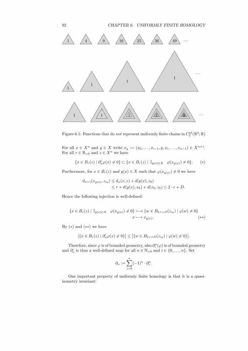
92 CHAPTER 6. UNIFORMLY FINITE HOMOLOGY
1 4 9 16 25 36 49 · · ·
11
11
· · ·
1 1 1 1 1 · · ·
Figure 6.1: Functions that do not represent uniformly finite chains in Cuf2 (R2;R)
For all x ∈ Xn and y ∈ X write xy := (x0, . . . , xi−1, y, xi, . . . , xn−1) ∈ Xn+1.For all r ∈ R>0 and z ∈ Xn we have
{x ∈ Br(z) | ∂inϕ(x) 6= 0} ⊂ {x ∈ Br(z) | ∃y(x)∈X ϕ(xy(x)) 6= 0}. (∗)
Furthermore, for x ∈ Br(z) and y(x) ∈ X such that ϕ(xy(x)) 6= 0 we have
dn+1(xy(x), zz0) ≤ dn(x, z) + d(y(x), z0)
≤ r + d(y(x), x0) + d(x0, z0) ≤ 2 · r +D.
Hence the following injection is well-defined:
{x ∈ Br(z) | ∃y(x)∈X ϕ(xy(x)) 6= 0} −→ {w ∈ B2·r+D(zz0) | ϕ(w) 6= 0}
x 7−→ xy(x). (∗∗)
By (∗) and (∗∗) we have
∣∣{x ∈ Br(z) | ∂inϕ(x) 6= 0}∣∣ ≤
∣∣{w ∈ B2·r+D(zz0) | ϕ(w) 6= 0}∣∣.
Therefore, since ϕ is of bounded geometry, also ∂ni (ϕ) is of bounded geometryand ∂in is thus a well-defined map for all n ∈ N>0 and i ∈ {0, . . . , n}. Set
∂n :=n∑
i=0
(−1)n · ∂ni .
One important property of uniformly finite homology is that it is a quasi-isometry invariant:

6.1. UNIFORMLY FINITE HOMOLOGY 93
Proposition 6.1.6 ([10, Proposition 2.1]). Let X and Y be metric spaces and Aa normed Abelian group.
(i) Let f : X −→ Y be a quasi-isometric embedding. Then f induces a chainmap
Cuf∗ (f ;A) : Cuf
n (X ;A) −→ Cufn (Y ;A)
c 7−→∑
y∈Y
( ∑
x∈f−1(y)
c(x)
)· y.
(ii) Let f, g : X −→ Y be two quasi-isometric embeddings, at bounded dis-tance from each other, that is, such that supx∈X dY (f(x), g(x)) < ∞.Then Cuf
∗ (f ;A) and Cuf∗ (g;A) are chain homotopic.
(iii) In particular, if f : X −→ Y is a quasi-isometry, the map induced by f inuniformly finite homology via Cuf
∗ (f ;A)
Huf∗ (f ;A) : Huf
∗ (X ;A) −→ Huf∗ (Y ;A)
is an isomorphism of graded Abelian groups. If A is a normed vectorspace, Huf
∗ (f ;A) is an isomorphism of graded vector spaces.
Definition 6.1.7. Let (X, d) be a metric space.
(i) We call (X, d) uniformly discrete if
∃r∈R>0 ∀x∈X |Br(x)| = 1.
(ii) We call (X, d) of bounded geometry if χX , and therefore every functionin ℓ∞(X), is of bounded geometry.
(iii) If (X, d) is both uniformly discrete and of bounded geometry, we say that(X, d) is a UDBG space.
The main example of UDBG spaces for us are finitely generated groups witha word metric:
Definition 6.1.8 (Word metric). Let G be a group with a finite generatingset S. The word metric on G with respect to S is the metric
dS : G×G −→ R
(g, h) 7−→ inf{n ∈ N | ∃s1,...,sn∈S∪S−1 g−1 · h = s1 · · · sn}.
Remark 6.1.9. A finitely generated group with a word metric is obviouslyuniformly discrete and of bounded geometry. The word metric structure on afinitely generated group is unique up to quasi-isometry, hence the uniformlyfinite homology of a finitely generated group is (up to canonical isomorphism,induced by the identity map) uniquely defined.
Definition 6.1.10. Let X be a UDBG space. We call X amenable if thereexists a sequence (Fi)i∈N of non-empty finite subsets, such that for all r ∈ R>0
limi→∞
|∂rFi|
|Fi|= 0.
Such a sequence (Fi)i∈N is called a Følner-sequence for X .

94 CHAPTER 6. UNIFORMLY FINITE HOMOLOGY
If G is a finitely generated group with a word metric, then G is amenable asa groupoid, Definition 4.1.3, if and only if it is amenable as a UDBG space [26,Theorem 4.9.2], see also Section 6.7.2. Block and Weinberger have shown, thatuniformly finite homology characterizes the amenability of a metric space:
Theorem 6.1.11 ([10, Theorem 3.1]). Let (X, d) be a uniformly discrete spaceof bounded geometry. Then the following are equivalent:
(i) The group Huf0 (X ;R) vanishes.
(ii) The fundamental class [χX ] ∈ Huf0 (X ;R) vanishes.
(iii) The space (X, d) is not amenable.
The following Proposition was noted by Brodzki, Niblo and Wright [12] forcoefficients in R, the proof is the same for any normed Abelian group, however:
Proposition 6.1.12 (Uniformly finite homology coincides with ℓ∞-homology).Let G be a finitely generated group and A a normed Abelian group. There is acanonical chain isomorphism
Cuf∗ (G;A) −→ C∗(G; ℓ∞(G,A)).
In particular, Huf∗ (G;A) ∼= H∗(G; ℓ∞(G,A)).
Here, the G-action on ℓ∞(G,A) is given
G× ℓ∞(G,A) −→ ℓ∞(G,A)
(g, ϕ) 7−→(h 7−→ ϕ(g−1 · h)
).
The idea of the proof is, that for each r ∈ N>0 and n ∈ N there are only finitelymany n-simplices having diameter smaller or equal r and 0-vertex e. Hence foreach c ∈ Cuf
n (G;A) there are only finitely many G-orbits in Gn+1 where c is notequal to 0 on the whole orbit. Thus, we can view c as a family of functions inℓ∞(G,A) over a finite subset of Gn+1 and this induces the chain isomorphism.See also Theorem 6.3.5 for the cohomological situation.
Corollary 6.1.13. Let G be a finitely generated group and A a normed Abeliangroup. Then uniformly finite homology in degree 0 is isomorphic to the spaceof coinvariants of ℓ∞(G,A), i.e.,
Huf0 (G;A) ∼= ℓ∞(G,A)G.
With the description of uniformly finite homology in terms of ℓ∞-homologyone can give a short and direct proof of the vanishing theorem of Block andWeinberger in the case of finitely generated groups:
Theorem 6.1.14 (0-degree uniformly finite homology and amenable groups,[12]). Let G be a finitely generated group. Then the following are equivalent:
(i) The 0-th uniformly finite homology Huf0 (G;R) vanishes.
(ii) The fundamental class [χG] ∈ Huf0 (G;R) vanishes.
(iii) The group G is not amenable.
6.2. TRANSFER AND COMPARISON MAPS 95
Proof. Clearly (i) implies (ii). By Corollary 6.1.13, the dual space H0(G;R)′ isisomorphic to HomG(ℓ∞(G),R). An invariant mean on G is by definition anelement m ∈ HomG(ℓ∞(G),R) such that m(χG) = 1, hence (ii) implies (iii).It is a simple fact that the set of invariant means spans HomG(ℓ∞(G),R) [69,Proposition 2.2], so (iii) implies (i).
We note the following fact since we will frequently use it in our examples:
Lemma 6.1.15. LetG be a finitely generated n-dimensional R-Poincare dualitygroup. Then Huf
k (G;R) = 0 for all k ∈ N>n and Hufn (G;R) ∼= R.
Proof. This follows directly from our identification of uniformly finite homologywith homology with coefficients in ℓ∞(G) and the fact that
Hufn (G;R) ∼= Hn(G; ℓ∞(G)) ∼= H0(G; ℓ∞(G)) ∼= ℓ∞(G)G ∼= R.
Motivated by Proposition 6.1.12, we will also use the following notation:
Definition 6.1.16. Let G be a group and A a normed Abelian group. Wewrite C∗
uf(G;A) := C∗(G; ℓ∞(G,A)) and call H∗uf(G;A) := H∗(C∗
uf(G;A)) theuniformly finite cohomology of G with coefficients in A.
6.2 Transfer and Comparison Maps
In this section, we discuss the comparison map between group homology anduniformly finite homology. If the group is amenable, each invariant mean inducesa transfer map, which is a left inverse to the comparison map. This fact will befundamental in Section 6.6. As an application, we demonstrate that the Hirschrank of a nilpotent group is a quasi-isometry invariant.
We will show that for n-dimensional groups, the comparison map is injectivein degree n and that for Poincare n-duality groups, the same holds in degreen− 1 as well. Using this we can calculate the uniformly finite homology of freegroups and surface groups.
Proposition 6.2.1. Let G be an amenable group. Then every left invariantmean m ∈M(G) induces a transfer map
m∗ : H∗(G; ℓ∞(G)) −→ H∗(G;R)
[c⊗ ϕ] 7−→ m(ϕ) · [c],
which is left inverse to the comparison map
cuf∗ : H∗(G;R) −→ H∗(G; ℓ∞(G))
[c] 7−→ [c⊗ χG],
induced by the canonical inclusion R −→ ℓ∞(G) as constant functions.
Proposition 6.2.1 follows directly from the following remark:
Remark 6.2.2. Let G be a group.

96 CHAPTER 6. UNIFORMLY FINITE HOMOLOGY
(i) By the short exact coefficient sequence of G-modules
0 −→ R −→ ℓ∞(G) −→ ℓ∞(G)/R −→ 0,
induced by the canonical inclusion R −→ ℓ∞(G) as constant functions, weget a long exact sequence in homology [15, Chapter III, Proposition 6.1]:
· · · −→ Hn(G;R) −→ Hn(G; ℓ∞(G)) −→ Hn(G; ℓ∞(G)/R) −→ · · ·
(ii) We call the map
cuf∗ : H∗(G;R) −→ H∗(G; ℓ∞(G))
[c] 7−→ [c⊗ χG],
induced by the canonical inclusion R −→ ℓ∞(G) as constant functions,the comparison map in uniformly finite homology. By a slight abuse ofnotation, we also write cuf∗ : H∗(G;R) −→ Huf
∗ (G;R) for the map inducedby the comparison map by Proposition 6.1.12.
(iii) Dually, the canonical inclusion R −→ ℓ∞(G) induces also a cohomologicalcomparison map
c∗uf : H∗(G;R) −→ H∗(G; ℓ∞(G)).
(iv) Let G be amenable. Every left G-invariant mean m : ℓ∞(G) −→ R splitsthe short exact coefficient sequence and hence we get for each n ∈ N asplit short exact sequence
0 Hn(G;R) Hn(G; ℓ∞(G)) Hn(G; ℓ∞(G)/R) 0.
Hn(G;m)
Corollary 6.2.3. Let G be a group of real cohomological dimension n ∈ N.
(i) The comparison map cufn is injective.
(ii) If G is a Poincare duality group, the comparison map cufn−1 is injective aswell.
Proof. This is follows directly from the long exact sequence of Remark 6.2.2,since Hn+1(G; ℓ∞(G)/R) = 0 and for a Poincare duality group
Hn(G; ℓ∞(G)/R) ∼= H0(G; ℓ∞(G)/R) ∼= (ℓ∞(G)/R)G.
But everyG-invariant element in ℓ∞(G) is constant, hence (ℓ∞(G)/R)G ∼= 0.
Using the identification of uniformly finite homology with ℓ∞-homology wenote:
Corollary 6.2.4. For any finitely generated amenable group G the comparisonmap H∗(G;R) −→ Huf
∗ (G;R) is injective.
6.2. TRANSFER AND COMPARISON MAPS 97
Example 6.2.5.
(i) Let Σ be a hyperbolic surface group. Then
dimRHufk (Σ;R) =
1 for k = 2
∞ for k = 1
0 else.
(ii) Let F be a non-Abelian free group. Then
dimRHufk (F ;R) =
{∞ for k = 1
0 else.
Proof. Both Σ and F are non-amenable, hence Huf0 (Σ;R) = 0 = Huf
0 (F ;R) byTheorem 6.1.14. A surface group is of course a 2-dimensional Poincare dualitygroup hence Huf
2 (Σ;R) ∼= R and Hufk (Σ;R) = 0 for k ∈ N>2 by Lemma 6.1.15.
Furthermore, F is a 1-dimensional group, so the only interesting case is k = 1.The group Σ contains a family (Σg)g∈Γ of finite index subgroups that are surfacegroups of arbitrarily large genus and F contains a family (Fg′)g′∈Γ′ of finiteindex subgroups that are free of arbitrarily large rank. For all these groups, thecomparison map in degree 1 is injective, hence we get inclusions for all g ∈ Γand g′ ∈ Γ′
H1(Σg;R) −→ Huf1 (Σg;R) ∼= Huf
1 (Σ;R)
H1(Fg′ ;R) −→ Huf1 (Fg′ ;R) ∼= Huf
1 (F ;R).
The isomorphisms follow from the quasi-isometry invariance of uniformly finitehomology. So dimRH
uf1 (F ;R) = ∞ = dimRH
uf1 (Σ;R).
Definition 6.2.6. The uniformly finite homological dimension of a group G isdefined as
hduf(G) = sup{n ∈ N
∣∣ Hufn (G;R) 6= 0
}∈ N ∪ {−∞,+∞}.
Since uniformly finite homology is invariant under quasi-isometry, we obtainthe following fact as a consequence of Proposition 6.2.1:
Corollary 6.2.7 ([9, Corollary 3.5]). The Hirsch rank of a finitely generatedvirtually nilpotent group G equals hduf(G). In particular, the Hirsch rank is aquasi-isometry invariant.
Proof. We can assume that G is nilpotent, since by definition the Hirsch rank ofa virtually nilpotent group is the Hirsch rank of any finite index nilpotent sub-group. Clearly, hduf(G) ≤ hdR(G), where hdR(G) denotes the real homologicaldimension of G by Proposition 6.1.12.
On the other hand, for a finitely generated nilpotent group the real homolog-ical dimension is equal both to the largest n ∈ N for which Hn(G;R) 6= 0 and toits Hirsch rank [73]. Since nilpotent groups are amenable, by Proposition 6.2.1,this integer must be smaller or equal than hduf(G).

98 CHAPTER 6. UNIFORMLY FINITE HOMOLOGY
6.3 ℓ∞-Cohomology and Bounded Cohomology
Bounded valued cohomology was introduced by Gersten [42, 44] and seen byGersten [43] and Mineyev [57] as a homological invariant that detects hyper-bolicity of groups, i.e., it vanishes in certain cases if and only if the group ishyperbolic:
Theorem 6.3.1 ([57, 43]). Let G be a finitely presented group. Then the fol-lowing are equivalent:
(i) The group G is hyperbolic.
(ii) For all normed R-modules V we have H2(∞)(G;V ) = 0 and G.
(iii) The group G is of type F∞ and for all normed R-modules V and forall n ∈ N≥2 we have Hn
(∞)(G;V ) = 0
Mineyev [59] proved a different cohomological characterisation of hyperbolicgroups in terms of the surjectivity of the comparison map in bounded coho-mology and in the same article asked about the relation between these twoinvariants:
Theorem 6.3.2 ([58, 59]). Let G be a finitely presented group. Then the fol-lowing are equivalent
(i) The group G is hyperbolic.
(ii) The comparison map c2b,V : H2b (G;V ) −→ H2(G;V ) is surjective for any
normed G-module V .
(iii) The comparison maps cnb,V : Hnb (G;V ) −→ Hn(G;V ) are surjective for
any n ∈ N≥2 and any normed G-module V .
Similarly to the situation for uniformly finite homology, we will show thatbounded valued cohomology of a group equals cohomology with ℓ∞-coefficients,hence bounded valued cohomology can be seen as a cohomological version ofuniformly finite homology.
Using this, we will study the relation between bounded valued cohomologyand bounded cohomology and show that Mineyev’s result on the surjectivity ofthe comparison map in bounded cohomology immediately implies the vanishingof bounded valued cohomology. Furthermore, combining this with the resultof Gersten, we directly see that surjectivity of the comparison maps implieshyperbolicity.
Bounded valued cohomology can be defined as a cellular version of boundedcohomology:
Definition 6.3.3. Let X be a CW-complex with finite n-skeleton for some n ∈N. Let V be a normed vector space.
(i) Consider the cellular chain complex (Ccell∗ (X;V ), ∂cell∗ )∗∈Z, endowed in
each degree with the ℓ1-norm with respect to the cellular basis. Define forall i ∈ {0, . . . , n}
Ci(∞)(X;V ) ⊂ Ci
cell(X ;V )
as the subspace of bounded cellular i-cochains, i.e., the subspace of alli-cochains that are bounded with respect to the ℓ1-norm.

6.3. ℓ∞-COHOMOLOGY AND BOUNDED COHOMOLOGY 99
(ii) The coboundary maps of C∗cell(X, V ) restrict to (Ci
(∞)(X ;V ))i∈{0,...,n},
turning it into a cochain complex over {0, . . . , n}.
(iii) For i ∈ {0, . . . , n− 1}, we call the corresponding cohomology Hi(∞)(X;V )
the bounded valued i-th cohomology group of X with coefficents in V .
Definition 6.3.4. Let n ∈ N and G be a group. Assume that there is a CW-complex X that is a model for BG such that X(n+1) is finite. Then we set
Hn(∞)(G;V ) := Hn
(∞)(X ;V ).
This is independent of the chosen model for BG by Corollary 6.3.6.
Similarly to the case of uniformly finite homology, bounded valued cohomol-ogy coincides with cohomology with ℓ∞-coefficients:
Theorem 6.3.5. Let n ∈ N and G be a group having a model of BG withfinite n-skeleton. Let V be a normed G-module. Then there is a canonicalisomorphism
Hk(G; ℓ∞(G, V )) −→ Hk(∞)(G;V )
for all k ∈ {0, . . . , n− 1}.
Proof. Choose a CW-complex X that is a model for BG such that X(n) is finite.Up to canonical isomorphism, we can describe H∗(G; ℓ∞(G, V )) as the cohomol-ogy of C∗
cell(X ; ℓ∞(G, V )) (with twisted coefficients). There is a (canonical) pairof mutually inverse cochain isomorphisms
α∗ : C∗cell(X ; ℓ∞(G, V )) −→ C∗
(∞)(X ;V )
ϕ 7−→(σ 7−→ ϕ(σ)(e)
)
β∗ : C∗(∞)(X;V ) −→ C∗
cell(X ; ℓ∞(G, V ))
ψ 7−→(σ 7−→
(g 7−→ ψ(g−1 · σ)
)).
• Consider ϕ ∈ Ckcell(X ; ℓ∞(G, V )) and k ∈ {0, . . . , n}. Then αk(ϕ) is a
bounded valued cochain, because: Let F (k) be a (finite) representative
system for the action of G on the k-cells of X . Then for all k-cells σ thereis a g ∈ G such that g · σ ∈ F (k); hence
|αk(ϕ)(σ)| = |ϕ(σ)(e)|
= |ϕ(g · σ)(g)|
≤ maxτ∈F (k)
‖ϕ(τ)‖∞
Therefore, we have
supσ∈Sk(X)
|αk(ϕ)(σ)| ≤ maxτ∈F (k)
‖ϕ(τ)‖∞ <∞.
• Consider ψ ∈ Ck(∞)(X;V ). Then for all k-cells σ the map βk(ψ)(σ) is
bounded, since for all g ∈ G
|βk(ψ)(σ)(g)| = |ψ(g−1 · σ)| ≤ ‖ψ‖∞ <∞.

100 CHAPTER 6. UNIFORMLY FINITE HOMOLOGY
• The map βk(ψ) is G-equivariant, since for all k cells σ and all h, g ∈ G
βk(ψ)(h · σ)(g) = ψ(g−1 · h · σ)
= βk(ψ)(σ)(h−1 · g)
= h · βk(ψ)(g).
• The maps α∗ and β∗ are cochain maps: For all k ∈ {0, . . . , n}, for all σ ∈
Ccellk+1(X;R) and all ϕ ∈ Ck
cell(X ;V )
δk(αk(ϕ))(σ) = αk(ϕ)(∂k+1σ)
= ϕ(∂k+1σ)(e)
= (δkϕ)(σ)(e)
= αk+1(δkϕ)(σ).
Similarly for β∗.
• For all k ∈ {0, . . . , n}, the maps αk and βk are obviously mutually inverse:
For all σ ∈ Ccellk (X ;R), all g ∈ G, all ϕ ∈ Ck
cell(X ; ℓ∞(G, V )) and all
ψ ∈ Ck(∞)(X;V ) we have
(αk ◦ βk)(ψ)(σ) = βk(ψ)(σ)(e) = ψ(σ)
and
(βk ◦ αk)(ϕ)(σ)(g) = αk(ϕ)(g−1 · σ) = ϕ(g−1 · σ)(e) = ϕ(σ)(g).
In particular, the definition of bounded valued cohomology is independentup to canonical isomorphism of the choice of the classifying space and the CW-structure on BG:
Corollary 6.3.6. Let n ∈ N and G be a group. Suppose X and Y are twomodels of BG with finite n-skeleton. Then there is a canonical isomorphism
Hk(∞)(X;V ) ∼= Hk
(∞)(Y ;V )
for all k ∈ {0, . . . , n− 1}.
Corollary 6.3.7. Let G be a hyperbolic group and V a normed R-module.Then G has a model X for BG such that X(k) is finite for all k ∈ N. Let V bea normed R-module. For all n ∈ N≥2 we have
Hn(∞)(G;V ) ∼= Hn(G; ℓ∞(G, V )) = 0.
Proof. The existence of such a model X is a well-known result [11, ChapterIII.Γ, Corollary 3.26]. By Theorem 6.3.2, the comparison map
cnb,ℓ∞(G,V ) : Hnb (G; ℓ∞(G, V )) −→ Hn(G; ℓ∞(G, V ))
is surjective. Since ℓ∞(G, V ) is relatively injective G-module, Hnb (G; ℓ∞(G, V ))
is trivial [62].
6.4. QUASI-MORPHISMS AND ℓ∞-COHOMOLOGY 101
The implication (ii) =⇒ (i) from Theorem 6.3.2 follows now directly fromGersten’s part of Theorem 6.3.1:
Corollary 6.3.8. Let G be a finitely presented group. If the comparison mapc2b,V : H2
b (G;V ) −→ H2(G;V ) is surjective for any normed G-module V , then Gis hyperbolic.
Proof. As in the proof of Corollary 6.3.7, we see that Hn(∞)(G;V ) = 0 for
all n ∈ N≥2, hence by Theorem 6.3.1, G is hyperbolic.
We have seen that the comparison map in bounded cohomology is surjectiveif and only if ℓ∞-cohomology vanishes (if considering all coefficients). Moreover,as we have noted in Section 6.2, the comparison map in ℓ∞-cohomology is in-jective for amenable groups and for these groups bounded cohomology vanishes.There is also the following relation between the comparison maps, noted byGersten for bounded valued cohomology, which in our language is now obvious:
Proposition 6.3.9. For n ∈ N>1 and all normed G-spaces V , the compositioncnuf,V ◦ cnb,V of the comparison maps is zero.
Proof. The following diagram commutes:
Hnb (G;V ) Hn
b (G, ℓ∞(G;V )) = 0
Hn(G;V ) Hn(G; ℓ∞(G, V ))cnuf,V
cnb,V cnb,ℓ∞(G,V )
Here, we use again that Hnb (G; ℓ∞(G, V )) is trivial since ℓ∞(G, V ) is relatively
injective, [62].
The examples mentioned above and Section 6.4 lead to the following ques-tions:
Question 6.3.10. Let G be a finitely generated group and n ∈ N. Under whichconditions on G is the sequence
Hnb (G;R) Hn(G;V ) Hn(G; ℓ∞(G, V ))
cnb,R cnuf,R
exact? Is there a long exact sequence that relates the comparison maps inbounded cohomology and bounded valued cohomology?
6.4 Quasi-Morphisms and ℓ∞-Cohomology
In this section we study the relation between quasi-morphisms and cohomologywith coefficients in ℓ∞. It turns out that this relation mirrors the situation inbounded cohomology.
102 CHAPTER 6. UNIFORMLY FINITE HOMOLOGY
Definition 6.4.1. Let G be a group. A quasi-morphism from G to R is amap ϕ : G −→ R such that
D(ϕ) := supa,b∈G
|ϕ(a · b) − ϕ(a) − ϕ(b)| <∞.
We call D(ϕ) the defect of ϕ. We call ϕ homogeneous if for all n ∈ N and g ∈ G
ϕ(gn) = n · ϕ(g).
and write Q(G) ⊂ Map(G,R) for the R-subspace of homogeneous quasi-mor-phisms.
Our result will be motivated by the following fact:
Theorem 6.4.2 ([25, Theorem 2.50]). For every group G there is an exactsequence
0 7−→ H1(G;R) −→ Q(G) −→ H2b (G;R) −→ H2(G;R).
The first map is given by the canonical inclusion
i : H1(G;R) ∼= Hom(G;R) −→ Q(G)
ϕ 7−→(g1 7−→ ϕ(1, g−1
1 )).
Proof. This is a well-known result that follows directly from the definition ofquasi-morphisms.
Now we can show that H1uf(G;R) detects quasi-morphisms fromG to R. This
result and its proof should be compared to the situation in bounded cohomologyas expressed by Theorem 6.4.2.
Proposition 6.4.3. For every group G, there is a canonical injection
c : Q(G) −→ H1uf(G;R),
such that c ◦ i = c1uf .
Proof. For all ϕ : G −→ R set
ϕ : G −→ Map(G,R)
g 7−→(h 7−→ ϕ(g−1 · h)
).
We then define the map
c′ : Q(G) −→ C1uf(G;R)
ϕ 7−→((g0, g1) 7−→ ϕ(g0 · g1) − ϕ(g0)
)= ϕ ◦ ∂1.
Now c′(ϕ) is G-equivariant since for all g, g0, g1, h ∈ G
c′(ϕ)(g · g0, g1)(h) = ϕ(g−11 g−1
0 (g−1h)) − ϕ(g−10 (g−1h)) = c′(ϕ)(g0, g1)(g−1h).

6.5. INTEGRAL AND REAL COEFFICIENTS 103
Furthermore, we have for all g0, g1 ∈ G
suph∈G
|ϕ(g0 · g1)(h) − ϕ(g0)(h)|
= suph∈G
|ϕ((g−11 · g−1
0 · h) − ϕ(g−10 · h)|
≤ suph∈G
|ϕ(g−11 · g−1
0 · h) − ϕ(g−10 · h) − ϕ(g−1
1 )| + |ϕ(g−11 )|
≤ D(ϕ) + |ϕ(g−11 )|.
Hence c′(ϕ)(g0, g1) ∈ ℓ∞(G). Obviously, for all ϕ ∈ Q(G) the image c′(ϕ)is a cocycle. Let c : Q(G) −→ H1
uf(G;R) be the map induced by c′. By asimilar calculation, we see that for ϕ ∈ Hom(G,R), i.e., D(ϕ) = 0, we havec(i(ϕ)) = [(g0, g1) 7−→ (h 7−→ ϕ(g1))] = c1uf(ϕ), hence c1uf = c ◦ i. We finallyshow that c is injective: Consider any pair ϕ ∈ Q(G) and ψ ∈ C0
uf(G) suchthat c′(ϕ) = δ1ufψ. Then
supg1∈G
|ϕ(g1)| = supg1∈G
|ϕ(g1) + ϕ(e) − ϕ(g1 · 1) − ϕ(e) + ϕ(g1 · 1)|
≤ supg0,g1∈G
(|ϕ(g1) + ϕ(g0) − ϕ(g0 · g1)| + |δ1ufψ(1, g−1
1 )(e)|)
= D(ϕ) + supg1∈G
|ψ(g−11 )(e) − ψ(1)(e)|
≤ D(ϕ) + 2‖ψ‖∞.
Thus ϕ : G −→ R is bounded and homogeneous, hence trivial.
Corollary 6.4.4. Let G be a hyperbolic R-Poincare duality group of dimen-sion n ∈ N>0. Then for k ∈ N
dimRHufk (G;R) =
1 for k = n
∞ for k = n− 1
0 else.
Proof. The vanishing for k ∈ {0, . . . , n − 1} is a consequence of duality andCorollary 6.3.7. Consider now k = n − 1. If G is quasi-isometric to Z, thisfollows from our calculation for amenable groups (Proposition 6.7.2). If G is notelementary hyperbolic, then Q(G) is infinite-dimensional by the result of Epsteinand Fujiwara [37], so by Proposition 6.4.3 it follows that dimRH
1uf(G;R) =
∞.
6.5 Integral and Real Coefficients
For some applications (e.g. Dranishnikov’s analysis of large-scale dimensions [34]or the quasi-isometry classification of certain group extensions by Kleiner andLeeb [52]) it is important to consider uniformly finite homology with coefficientsin Z. The description in terms of ℓ∞-homology allows us to present conciselywhat is known about the relation between coefficients in Z and in R. Further-more, we discuss an important geometric characterisation for a class in degree0 to be trivial. We basically follow Whyte [78] in this section.

104 CHAPTER 6. UNIFORMLY FINITE HOMOLOGY
Proposition 6.5.1. Let G be a finitely generated group.
(i) Let
0 −→ Ai
−→ Bp
−→ C −→ 0
be a short exact sequence of normed abelian groups and σ : C −→ B abounded, not necessarily linear, splitting. Then there is an induced longexact sequence:
· · · Hufn (G;A) Huf
n (G;B) Hufn (G;C) Huf
n−1(G;A) · · ·
(ii) In particular, there is a long exact sequence:
· · · Hufn (G;Z) Huf
n (G;R) Hufn (G;R/Z) Huf
n−1(G;Z) · · ·
Proof. Applying ℓ∞ to the coefficient sequence induces a short exact sequenceof normed G-modules:
0 −→ ℓ∞(G,A) −→ ℓ∞(G,B) −→ ℓ∞(G,C) −→ 0.
The only non-obvious part is the surjectivity of ℓ∞(G,B) −→ ℓ∞(G,C) and thisfollows from the existence of the splitting. Thus we get a long exact sequencein homology.
A splitting for the second part is given by mapping each class in R/Z to itsrepresentative in [0, 1).
Corollary 6.5.2. Let G be an infinite finitely generated group. Then thechange-of-coefficients map Huf
0 (G;Z) −→ Huf0 (G;R) is surjective.
Proof. We only have to show that Huf0 (G,R/Z) ∼= 0. But uniformly finite
homology of an infinite group with bounded coefficients vanishes in degree 0,since: In an infinite group, one can always find a locally finite family (tg)g∈G
of proper edge path rays (“tails”), such that ∂1tg = g for all g ∈ G. Since thethe coefficient module R/Z is bounded, the formal sum
∑g∈G tg is a uniformly
finite 1-chain, whose boundary is the fundamental class [χG]. This is similar tothe argument in [10, Lemma 2.4].
Definition 6.5.3. Let G be a finitely generated discrete group with a wordmetric d. For any S ⊂ G and r ∈ R>0 set
∂r(S) := {g ∈ G∣∣ 0 < d(g, S) ≤ r}.
The following Theorem of Whyte gives a geometric characterisation of thevanishing of zero cycles in uniformly finite homology:
Theorem 6.5.4 ([78, Theorem 7.7]). Let G be a finitely generated group. Acycle c ∈ Cuf
0 (G;Z) is trivial in Huf0 (G;Z) if and only if
∃C, r∈N>0 ∀S⊆G finite
∣∣∣∣∣∑
s∈S
c(s)
∣∣∣∣∣ ≤ C · |∂rS|. (W)

6.5. INTEGRAL AND REAL COEFFICIENTS 105
We will give a short proof of the fact that condition (W) in Theorem 6.5.4is necessary for a cycle to vanish that works both for and coefficients in Z andin R:
Proof that vanishing of a cycle implies condition (W). Let c ∈ Cuf0 (G;Z) be a
boundary. Consider a chain b ∈ Cuf1 (G;Z) such that ∂uf1 b = c. Choose r ∈ R>0
such that b(g0, g1) = 0 for all g0, g1 ∈ G with d(g0, g1) ≥ r. Set C := ‖c‖∞.If S ⊂ G is a finite subset in G, the points in ∂rS are the only points in G\S thatcan be reached by edges in the support of b starting in S, i.e., if b(g0, g1) 6= 0and g0 ∈ S, then g1 ∈ ∂rS ∪ S, Figure 6.5, hence
∣∣∣∣∣∑
s∈S
c(s)
∣∣∣∣∣ ≤∑
s∈∂rS
|c(s)| ≤ C · |∂rS|.
The proof is the same for R-coefficients.
S
r
g0
g1
b(g0, g1)
Figure 6.2: Whyte’s vanishing criterion
Whyte stated Theorem 6.5.4 only for coefficients in Z, but it is now clearthat it also holds for coefficients in R:
Corollary 6.5.5. Theorem 6.5.4 also holds if one replaces Z by R.
Proof. Let c ∈ Cuf0 (G;R) be a cycle. We have already seen that condition (W) is
necessary for the class [c] to be trivial in Huf0 (G;R). Assume that c satisfies (W)

106 CHAPTER 6. UNIFORMLY FINITE HOMOLOGY
for some C, r ∈ R>0. Let i : C0(G;Z) −→ C0(G;R) denote the change-of-coefficients map. By Corollary 6.5.2, there is a cycle cint ∈ Cuf
0 (G;Z) suchthat [c− i(cint)] = 0 in Huf
0 (G;R). Hence c− i(cint) also satisfies (W) for someconstants C′, r′ ∈ R>0. Thus for all finite subsets S ∈ G and r′′ := max{r, r′}and C′′ := C + C′
∣∣∣∣∣∑
s∈S
cint(s)
∣∣∣∣∣ ≤∣∣∣∣∣∑
s∈S
c(s)
∣∣∣∣∣ +
∣∣∣∣∣∑
s∈S
(c− i(cint))(s)
∣∣∣∣∣
≤ C · |∂rS| + C′ · |∂r′S|
≤ C′′ · |∂r′′S|.
Hence [cint] is trivial in Huf0 (G;Z) by Theorem 6.5.4 and therefore also [c] = 0
in Huf0 (G;R).
Corollary 6.5.6 ([78, Lemma 7.7]). Let G be a finitely generated group. Thenthe change-of-coefficients map Huf
0 (G;Z) −→ Huf0 (G;R) is an isomorphism.
Proof. It is surjective by Corollary 6.5.2 and injective by Theorem 6.5.4 andCorollary 6.5.5.
The following corollary was noted by Gersten for bounded valued cohomol-ogy:
Corollary 6.5.7. Let G be a finitely generated Poincare duality group of di-mension n ∈ N. Then for all k ∈ {0, . . . , n− 1} the change-of-coefficients map
Hufk (G;Z) −→ Huf
k (G;R)
is an isomorphism.
Proof. The module R/Z is bounded, hence
ℓ∞(G,R/Z) = Map(G,R/Z) ∼=ZG Hom(ZG,R/Z).
So for all k ∈ {0, . . . , n− 1}
Hufk (G;R/Z) ∼= Hn−k(G; ℓ∞(G,R/Z))
∼= Hn−k(G; Hom(ZG,R/Z))
= 0.
The last equality follow because Hom(ZG;R/Z) is an injective G-module [15,Proposition 6.1].
6.6 Uniformly Finite Homology and AmenableGroups
In this section we present the main result of joint work with Francesca Dianaabout uniformly finite homology of amenable groups [9]. We will only give asummary here, for a more detailed treatment confer the article. If G is anamenable group, write LM(G) ⊂ ℓ∞(G)′ for the space of left invariant meansand M(G) for the space of bi-invariant means on G.

6.6. UNIFORMLY FINITE HOMOLOGY AND AMENABLE GROUPS 107
We will show that uniformly finite homology groups of amenable groups areoften infinite dimensional. Our principal observation is the following: Let Gbe an infinite amenable group. On the one hand, by Proposition 6.2.1 everymean m on G induces a left inverse
m∗ : H∗(G; ℓ∞(G)) −→ H∗(G;R)
[c⊗ ϕ] 7−→ m(ϕ) · [c]
to the comparison map. On the other hand, there are many candidates for thesesplitting maps, since by the following classical result of Chou [28, Theorem 1]there are many different invariant means:
Theorem 6.6.1. If G is an infinite amenable group, then G has exactly 22|G|
left invariant means, where |G| denotes the cardinality of G. Thus LM(G) isinfinite dimensional.
The main idea is to use the maps induced by different means to differenti-ate between different classes. In general, however, there might not be enoughcycles to be separated by means, e.g. Huf
n (Zn;R) ∼= R and all the func-tions mn : Huf
n (Zn;R) −→ Hn(Zn;R) induced by means coincide. The problemis that for a cycle c ∈ Cn(G;R) and a bounded function ϕ ∈ ℓ∞(G;R), thechain c ⊗ ϕ ∈ Cn(G; ℓ∞(G;R)) is not necessarily a cycle since the G-actionon ℓ∞(G;R) is not trivial.
We avoid this issue by considering cycles c ∈ Cn(G;R) that are supported ina subgroup H ≤ G and functions ϕ ∈ ℓ∞(G;R) that are invariant with respectto the action of H . Then c⊗ ϕ ∈ Cn(G; ℓ∞(G;R)) will be a cycle as well.
The next step is to show that, if H ≤ G has infinite index, then we canfind an infinite family of different G-invariant means that can be separated byH-invariant functions, a result that might be of independent interest:
Theorem 6.6.2 ([9, Theorem 3.11]). Let G be a finitely generated amenablegroup and H ≤ G a subgroup such that [G : H ] = ∞. Then there exists an infi-nite family (mj)j∈J of left G-invariant means and an infinite family (fj)j∈J of
(left) H-invariant functions in ℓ∞(G), such that mk(fj) = δk,j for any k, j ∈ J .
Sketch of proof. We can inductively construct a family (Alk)k,l∈N (Figure 6.3)
of subsets in G such that:
• For each (k, l) ∈ N2, the set Alk is a (right-translated) l-Ball, i.e., there
exists a g ∈ G such thatAl
k = Bl(e) · g.
• Their orbits under left-translation by elements in H are disjoint, i.e., foreach pair of distinct indices (k, l) 6= (k′, l′) ∈ N2
(H ·Al
k
)∩(H ·Al′
k′
)= ∅.
For each k ∈ N setT k :=
⋃
l∈N
H ·Alk.
The family (T k)k∈N is pairwise disjoint and the corresponding characteristicfunctions χTk are H-invariant for each k ∈ N. Using the correspondence be-tween Følner-sequences and means, we can construct a sequence (mj)j∈N ofG-invariant means such that mj is supported in T j.

108 CHAPTER 6. UNIFORMLY FINITE HOMOLOGY
A11 A2
1 A12 A2
2 A31 A1
3
Z× {0}
{0} × Z
Figure 6.3: Constructing a family of disjoint (Z × {0})-invariant subsets sup-porting invariant means in Z2
Hence, if there is a cycle c ∈ Cn(H ;R) such that [in(c)] ∈ Hn(G;R) is nottrivial, then ([i(c)⊗fj])j∈J is a family of linear independent classes in Huf
n (G;R)(with fj as in Theorem 6.6.2 and i : H −→ G the canonical inclusion). There-fore, we have proven:
Theorem 6.6.3 ([9, Theorem 3.8]). Let G be a finitely generated amenablegroup. Let H ≤ G be an infinite index subgroup. For each n ∈ N such that themap
Hn(i;R) : Hn(H ;R) −→ Hn(G;R)
induced by the inclusion i : H −→ G is non-trivial, dimRHufn (G;R) = ∞ holds.
There are trivial reasons for uniformly finite homology to be finite dimen-sional that we will also see in some of our examples:
Lemma 6.6.4. Let G be virtually an n-dimensional R-Poincare duality group.Then Huf
k (G;R) = 0 for all k ∈ N>n and Hufn (G;R) ∼= R.
Proof. Since uniformly finite homology is a quasi-isometry invariant, after pass-ing to a finite index subgroup, we can assume that G is a Poincare dualitygroup. The vanishing of homology in higher degrees is part of the definition ofa Poincare duality group. In the top dimensional case we have
Hufn (G;R) ∼= Hn(G; ℓ∞(G)) ∼= H0(G; ℓ∞(G)) ∼= ℓ∞(G)G ∼= R.
We proceed to discuss several applications of Theorem 6.6.3. We start withthe situation in degree 1:
Corollary 6.6.5. Let G be a finitely generated amenable group, such that thefirst homology group H1(G;R) is non-trivial, i.e., that the abelianization of Gis not a torsion group. Then
dimRHuf1 (G;R) =
{1 if G is virtually Z
∞ otherwise.
6.6. UNIFORMLY FINITE HOMOLOGY AND AMENABLE GROUPS 109
Sketch of Proof. Pick any g ∈ G such that the image of g in Gab has infiniteorder. Either H := 〈g〉 ≤ G has finite index and G is virtually Z or H satisfiesthe conditions of Theorem 6.6.3 in degree 1 by the naturality of the isomor-phism H1(G;R) ∼= Gab ⊗ R.
Corollary 6.6.6 ([9, Example 4.4]). Let G be a finitely generated virtuallynilpotent group of Hirsch rank h ∈ N. Then
dimRHufk (G;R) =
1 if k = h
∞ if k ∈ {0, . . . , h− 1}
0 else.
Sketch of Proof. Using the calculation of the homology groups of finitely gener-ated nilpotent groups by Baumslag, Miller and Short [4], we can show that Ghas an infinite index subgroup H ≤ G satisfying the conditions in Theorem 6.6.3for k ∈ {0, . . . , h− 1}. The other cases follow because G is virtually a Poincareduality group.
Example 6.6.7 ([9, Example 4.2]). Let G,H be finitely generated infiniteamenable groups, such that that Hk(H ;R) 6= 0 for a k ∈ N. Then
dimRHufk (G⋊H ;R) = ∞.
In particular, for all l ∈ N
dimRHufk (Zl;R) =
1 if k = l
∞ if k ∈ {0, . . . , l − 1}
0 else.
Example 6.6.8 ([9, Example 4.5]). Consider A ∈ SL(2,Z). Then for the semi-direct product Z2 ⋊A Z given by the action of Z on Z2 induced by A, we have
dimRHufk (Z2 ⋊A Z;R) =
1 if k = 3
∞ if k ∈ {0, 1, 2}
0 else.
In particular, this example includes cocompact lattices in Sol [70] and the inte-gral three-dimensional Heisenberg group.
Using the work of Fujiwara and Oshika on the bounded cohomology of 3-manifold groups and our calculation in the amenable case, we get:
Theorem 6.6.9. Let M be a closed irreducible 3-manifold with fundamentalgroup G := π1(M). Then either G is finite or
dimRHuf2 (G;R) = ∞.
Proof. By the calculation of the second bounded cohomology of 3-manifoldsof Fujiwara and Oshika [41], either H2
b (G;R) is infinite dimensional or G isvirtually solvable. In the first case, the space of quasi-morphism Q(G) is infinitedimensional and so is H1
uf(G;R) by Proposition 6.4.3. By assumption and thesphere theorem [67, 77], after possibly passing to an orientable cover, we can
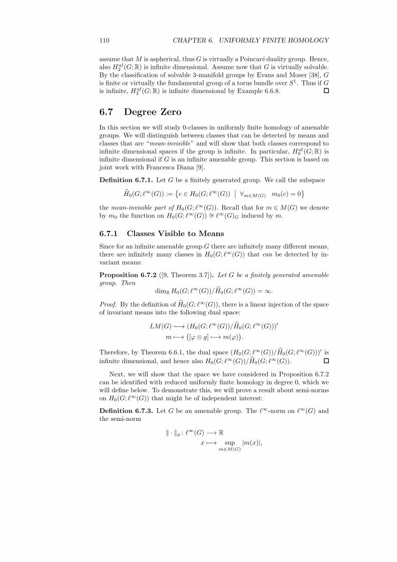
110 CHAPTER 6. UNIFORMLY FINITE HOMOLOGY
assume thatM is aspherical, thusG is virtually a Poincare duality group. Hence,also Huf
2 (G;R) is infinite dimensional. Assume now that G is virtually solvable.By the classification of solvable 3-manifold groups by Evans and Moser [38], Gis finite or virtually the fundamental group of a torus bundle over S1. Thus if Gis infinite, Huf
2 (G;R) is infinite dimensional by Example 6.6.8.
6.7 Degree Zero
In this section we will study 0-classes in uniformly finite homology of amenablegroups. We will distinguish between classes that can be detected by means andclasses that are “mean-invisible” and will show that both classes correspond toinfinite dimensional spaces if the group is infinite. In particular, Huf
0 (G;R) isinfinite dimensional if G is an infinite amenable group. This section is based onjoint work with Francesca Diana [9].
Definition 6.7.1. Let G be a finitely generated group. We call the subspace
H0(G; ℓ∞(G)) :={c ∈ H0(G; ℓ∞(G))
∣∣ ∀m∈M(G) m0(c) = 0}
the mean-invisible part of H0(G; ℓ∞(G)). Recall that for m ∈M(G) we denoteby m0 the function on H0(G; ℓ∞(G)) ∼= ℓ∞(G)G induced by m.
6.7.1 Classes Visible to Means
Since for an infinite amenable group G there are infinitely many different means,there are infinitely many classes in H0(G; ℓ∞(G)) that can be detected by in-variant means:
Proposition 6.7.2 ([9, Theorem 3.7]). Let G be a finitely generated amenablegroup. Then
dimRH0(G; ℓ∞(G))/H0(G; ℓ∞(G)) = ∞.
Proof. By the definition of H0(G; ℓ∞(G)), there is a linear injection of the spaceof invariant means into the following dual space:
LM(G) −→ (H0(G; ℓ∞(G))/H0(G; ℓ∞(G)))′
m 7−→([ϕ⊗ g] 7−→ m(ϕ)
).
Therefore, by Theorem 6.6.1, the dual space (H0(G; ℓ∞(G))/H0(G; ℓ∞(G)))′ is
infinite dimensional, and hence also H0(G; ℓ∞(G))/H0(G; ℓ∞(G)).
Next, we will show that the space we have considered in Proposition 6.7.2can be identified with reduced uniformly finite homology in degree 0, which wewill define below. To demonstrate this, we will prove a result about semi-normson H0(G; ℓ∞(G)) that might be of independent interest:
Definition 6.7.3. Let G be an amenable group. The ℓ∞-norm on ℓ∞(G) andthe semi-norm
‖ · ‖µ : ℓ∞(G) −→ R
x 7−→ supm∈M(G)
|m(x)|,

6.7. DEGREE ZERO 111
induce two semi-norms on H0(G; ℓ∞(G)) that we will also denote by ‖ · ‖∞and ‖ · ‖µ. Since every mean vanishes on im ∂uf1 , we have ‖ϕ‖µ = ‖[ϕ]‖µ forall ϕ ∈ Cuf
0 (G;R) .
Proposition 6.7.4. Let G be an amenable group. Then the semi-norms ‖ · ‖∞and ‖ · ‖µ on H0(G; ℓ∞(G)) are equivalent.
Proof. Clearly, (ℓ∞(G)G)′ ∼= BG(ℓ∞(G),R) and we will identify these spaceshere. Every functional in BG(ℓ∞(G),R) can be written as the difference of twopositive functionals in BG(ℓ∞(G),R) [69, Proposition 2.2]. The claim about thenorms is then a classical result, we recall a proof from [50, Theorem 23.2]:
Clearly, ‖ · ‖µ ≤ ‖ · ‖∞ on ℓ∞(G) and hence also on H0(G; ℓ∞(G)). Wewrite P1 := {λ ·m | m ∈ M(G), λ ∈ [0, 1]} for the set of positive functionalsof norm smaller or equal 1 in BG(ℓ∞(G),R). As we have noted above, everyfunction f ∈ (ℓ∞(G)G)′ ∼= BG(ℓ∞(G),R) can be written as
f = r · (ϕ1 − ϕ2)
with r ∈ R>0 and ϕ1, ϕ2 ∈ P1. Since {ϕ1 − ϕ2 | ϕ1, ϕ2 ∈ P1} is weak-∗-closed and convex, by the weak-∗-compactness of the unit ball, there exists aconstant R ∈ R>0 such that every f ∈ (ℓ∞(G)G)′ with ‖f‖∞ ≤ 1 can be writtenas
f = R · (ϕ1 − ϕ2).
By the Hahn-Banach-Theorem, we have for all x ∈ ℓ∞(G)G
‖x‖∞ = sup{|f(x)|
∣∣ f ∈ (ℓ∞(G)G)′, ‖f‖∞ ≤ 1},
hence
‖x‖∞ ≤ sup{|R · (ϕ1(x) − ϕ2(x))| | ϕ1, ϕ2 ∈ P1}
≤ 2 · R · sup{|ϕ(x)| | ϕ ∈ P1}
= 2 · R · sup{|m(x)| | m ∈M(G)}
= 2 · R · ‖x‖µ.
Proposition 6.7.4 implies directly the following correspondence between clas-ses that can be detected by means and reduced uniformly finite homology, thatwas told to us by Micha l Marcinkowski:
Corollary 6.7.5 ([69, Proposition 2.1]). Let G be an amenable group. Then
{v − g · v | v ∈ ℓ∞(G), g ∈ G}‖·‖ℓ∞
= {c ∈ ℓ∞(G) | ∀m∈M(G) m(c) = 0}.
In other words, if
Huf
0 (G;R) := Cuf0 (G;R)/im ∂uf1
‖ ‖ℓ∞
is the reduced 0th-uniformly finite homology group, we have
Huf
0 (G;R) ∼= H0(G; ℓ∞(G))/H0(G; ℓ∞(G)).
In particular, Huf
0 (G;R) is infinite dimensional if G is an infinite amenablegroup.

112 CHAPTER 6. UNIFORMLY FINITE HOMOLOGY
Proof. An element ϕ ∈ ℓ∞(G) is in {c ∈ ℓ∞(G) | ∀m∈M(G) m(c) = 0} if andonly if ‖[ϕ]‖µ = ‖ϕ‖µ = 0, hence if and only if ‖[ϕ]‖∞ = 0. Therefore
{v − g · v | v ∈ ℓ∞(G), g ∈ G}‖ ‖ℓ∞
= {c ∈ ℓ∞(G) | ∀m∈M(G) m(c) = 0}.
That Huf
0 (G;R) is infinite dimensional follows now from Proposition 6.7.2.
6.7.2 Distinguishing Classes by Asymptotic Behaviour
We will reformulate White’s criterion for the vanishing of 0-degree uniformlyfinite homology classes, Corollary 6.5.5, in terms of the asymptotic behaviourof chains in degree 0 with respect to the behaviour of a Følner-sequence. Wewill first need a notion to compare the asymptotic behaviour of functions:
Definition 6.7.6. Let α, β : N −→ R≥0 be two functions.
(i) We say β dominates α and write α ≺ β if β(n) is zero for at most finitelymany n ∈ N and
limn→∞
α(n)
β(n)= 0.
(ii) We write α ∼ β if β(n) is zero for at most finitely many n ∈ N and
limn→∞
α(n)
β(n)∈ R>0,
or if both α(n) and β(n) are zero for almost all n ∈ N.
(iii) Finally, we also write α � β if α ≺ β or α ∼ β.
Definition 6.7.7. Let G be a finitely generated group with a fixed word metric.A Følner sequence in G is a sequence (Sj)j∈N of non-empty finite subsets of Gsuch that for each r ∈ N>0
limj→∞
|∂r(Sj)|
|Sj |= 0.
Definition 6.7.8. Let S := (Sj)j∈N be a Følner-sequence in G. Consider thesequence of (not necessarily invariant) means (mj)j∈N given by
mj : ℓ∞(G) −→ R
ϕ 7−→1
|Fj |
∑
g∈Fj
ϕ(g).
We call S simple if (mj)j∈N weak-∗-converges in ℓ∞(G)′. In this case, write mS
for the weak-∗-limit of (mj)j∈N. The limit mS is always an invariant mean [26,Theorem 4.9.2].
Since the space of means is weak-∗-compact, every Følner sequence has asimple subsequence.

6.7. DEGREE ZERO 113
Definition 6.7.9. Let G be a finitely generated group and S := (Sj)j∈N aFølner sequence for G. For all c ∈ ℓ∞(G) we define a function
βSc : N −→ R
n 7−→|∑
s∈Snc(s)|
|Sn|.
Finally, we also consider the asymptotic behaviour of the boundaries given bythe function
σS : N −→ R
n 7−→|∂1Sn|
|Sn|.
Lemma 6.7.10 ([9, Lemma 5.6]). Let G be a finitely generated amenable groupand S a Følner sequence in G. Consider c ∈ ℓ∞(G).
(i) We have 0 � βSc � 1.
(ii) If S is simple, then βSc ∼ 1 if and only if mS(c) 6= 0. In particular, βS
c ∼ 1implies that there is a simple subsequence S′ of S such that mS′(c) 6= 0.
(iii) If βSc ≻ σS , then [c] 6= 0 ∈ Huf
0 (G;R).
(iv) Conversely, if [c] 6= 0 ∈ Huf0 (G;R) then there exists a Følner sequence S′
such that σS′ ≺ βS′
c .
(v) More generally: If (cn)n∈N is a sequence in ℓ∞(G) such that σS ≺ βSc0 and
∀n∈N βScn ≺ βS
cn+1,
then the family ([cn])n∈N of classes in Huf0 (G;R) is linearly independent.
Proof.
(i) This is clear by the definition of βSc .
(ii) If S is simple, the sequence (|∑
s∈Snc(s)|/|Sn|)n∈N, that we have to con-
sider to decide whether βSc ∼ 1, converges to |mS(c)|.
(iii) Assume [c] = 0. By Whyte’s criterion, Corollary 6.5.5, there exist C, r ∈N>0 such that for all n ∈ N
|∂1Sn|∣∣∑s∈S c(s)
∣∣ ≥1
|Br(e)|·
|∂rSn|∣∣∑s∈S c(s)
∣∣ ≥1
C · |Br(e)|> 0
Hence βSc 6≻ σS .
(iv) By Whyte’s criterion, if [c] 6= 0, for each n ∈ N there exists a finitesubset S′
n ⊆ G such that
n · |∂1S′n| <
∣∣∣∑
s∈S′n
c(s)∣∣∣;

114 CHAPTER 6. UNIFORMLY FINITE HOMOLOGY
hence
1
‖c‖∞·|∂1S′
n|
|S′n|
≤|∂1S′
n|∣∣∣∑
s∈S′nc(s)
∣∣∣<
1
n.
In particular S′ := (S′n)n∈N is a Følner sequence and σS′ ≺ βS′
c .
(v) For each c ∈ ℓ∞(G), such that∑
s∈Snc(s) is zero for at most finitely many
n ∈ N, we define a subspace
Cuf0 (G;R)�c :=
{c′ ∈ Cuf
0 (G;R)
∣∣∣∣ limn→∞
∑s∈Sn
c′(s)∑s∈Sn
c(s)exists
}.
Choose a splitting of R-vector spaces Cuf0 (G;R) = Cuf
0 (G;R)�c ⊕ V anddefine a linear function
γSc : Cuf0 (G;R) = Cuf
0 (G;R)�c ⊕ V −→ R
(c′, c′′) 7−→ limn→∞
∑s∈Sn
c′(s)∑s∈Sn
c(s).
Let a ∈ Cuf0 (G;R) be a boundary. Then the function βS
a /σS is boundedby Whyte’s criterion, so βS
a ≺ σS . Thus if σS ≺ βSc then βS
a ≺ βSc and
hence γSc (a) = 0. Therefore, γSc induces a linear map
γSc : Huf0 (G;R) −→ R.
In our situation we have γSci(cj) = δij for all j ≤ i in N. Hence, ([cn])n∈N
is linearly independent.
Notation 6.7.11. For each k ∈ N set [nk] := {mk | m ∈ N}.
Example 6.7.12. Consider the Følner sequence B in Z given by the sequenceof balls ({−n,−n+ 1, . . . , n})n∈N. Then for each k ∈ N>0
βB[nk] ∼
(m 7−→ m1−k
).
In particular, the sequence([nk])k∈N>0 of subsets in Z satisfies the conditions in
Lemma 6.7.10 (v) and hence induces a sequence of linearly independent classesin Huf
0 (Z;R).
Different Følner sequences can of course detect different classes:
Example 6.7.13. Consider the Følner sequence T in Z given by the sequenceof balls ({−n− 1,−n, . . . ,−1})n∈N. Then βT
[nk] ∼ 0 for each k ∈ N>0.
6.7.3 Sparse Classes
We now introduce a geometric condition for a subset to be mean-invisible:
Definition 6.7.14. Let G be a finitely generated group. We call a subset Γ ⊆ G(asymptotically) sparse (Figure 6.4) if
∃C∈N ∀r∈N>0 ∃R∈N>0 ∀g∈G\BR(e) |Γ ∩Br(g)| ≤ C.
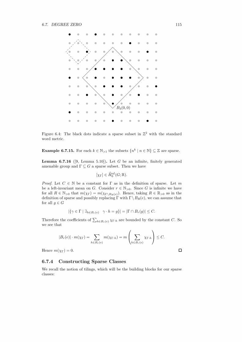
6.7. DEGREE ZERO 115
B3(0, 0)
Figure 6.4: The black dots indicate a sparse subset in Z2 with the standardword metric.
Example 6.7.15. For each k ∈ N>1 the subsets {nk | n ∈ N} ⊆ Z are sparse.
Lemma 6.7.16 ([9, Lemma 5.10]). Let G be an infinite, finitely generatedamenable group and Γ ⊆ G a sparse subset. Then we have
[χΓ] ∈ Huf0 (G;R).
Proof. Let C ∈ N be a constant for Γ as in the definition of sparse. Let mbe a left-invariant mean on G. Consider r ∈ N>0. Since G is infinite we havefor all R ∈ N>0 that m(χΓ) = m(χΓ\BR(e)). Hence, taking R ∈ R>0 as in thedefinition of sparse and possibly replacing Γ with Γ\BR(e), we can assume thatfor all g ∈ G
|{γ ∈ Γ | ∃h∈Br(e) γ · h = g}| = |Γ ∩Br(g)| ≤ C.
Therefore the coefficients of∑
h∈Br(e)χΓ·h are bounded by the constant C. So
we see that
|Br(e)| ·m(χΓ) =∑
h∈Br(e)
m(χΓ·h) = m
∑
h∈Br(e)
χΓ·h
≤ C.
Hence m(χΓ) = 0.
6.7.4 Constructing Sparse Classes
We recall the notion of tilings, which will be the building blocks for our sparseclasses:

116 CHAPTER 6. UNIFORMLY FINITE HOMOLOGY
Definition 6.7.17. Let G be a finitely generated group with a word metric.For r ∈ N>0 we call a subset T ⊆ G an r-tiling for G if
(i) ∀g1,g2∈T Br(g1) ∩Br(g2) 6= ∅ =⇒ g1 = g2
(ii) G =⋃
g∈T B2·r(g).
By Zorn’s Lemma, for all r ∈ N>0 there exists an r-tiling [26, Proposition 5.6.3].
Lemma 6.7.18 ([26, Proposition 5.6.4]). Let G be a finitely generated ame-nable group and (Sj)j∈N a Følner sequence. Let r ∈ N>0 and let T be an r-tilingfor G. Set
Tj := {g ∈ T | Br(g) ⊆ Sj} ⊆ Sj .
Then there exists an l(T ) ∈ N such that for all j ≥ l(T )
1
2 · |B2·r(e)|≤
|Tj|
|Sj |.
Sketch of proof. One obviously gets the corresponding estimate for the pointsin the (2 · r)-interior of Sj . But the number of points in the r-boundary of Sj
relative to |Sj | goes to zero for j → ∞.
The next theorem tells us that we can realise any non-trivial asymptoticbehaviour by a sparse set. This result is a stronger version of [9, Theorem 5.1]and the proof is simpler.
Theorem 6.7.19. Let G be a finitely generated infinite amenable group with aword metric. Then there is a Følner sequence S in G such that for each growthfunction c : N −→ R>0 such that c ≺ 1, there is a sparse subset Γ ⊂ G suchthat βS
Γ ∼ c. In particular, there is an uncountable family of linear independentsparse classes in Huf
0 (G;R).
Proof. Choose an r-tiling T r for all r ∈ N>0. Let S be a Følner sequence suchthat for all j ∈ N
d( j⋃
l=0
Sl, Sj+1
)> j. (∗)
For instance, start with an arbitrary Følner sequence and inductively translatethe j-th set away from the first j − 1 sets. Let c : N −→ R>0 be a growthfunction with c ≺ 1. Without changing the asymptotic behaviour of c, we canassume that c(r) ≤ |Sr| for all r ∈ N. For each r ∈ N>0 define a number
ρ(r) := max{r′ ∈ N
∣∣∣ c(r) ≤ |T r′
r |
|Sr|
}∈ N>0.
Since c ≺ 1, i.e., limr→∞ c(r) = 0, for all r′ ∈ N we can find an R ∈ N>0 suchthat for all r ∈ N≥R we have
c(r) <1
2 · |B2·r′(e)|
and
r ≥ max{l(T 0), . . . , l(T r′)}.

6.7. DEGREE ZERO 117
Therefore, by Lemma 6.7.18 we see that limr→∞ ρ(r) = ∞. We have
c(r) ≤|T
ρ(r)r |
|Sr|,
hence we can find a subset Lr ⊂ Tρ(r)r , such that
c(r) ≤|Lr|
|Sr|≤ c(r) +
1
|Sr|. (∗∗)
Set Γ :=⋃
r∈N>0Lr. By (∗∗) we have c ∼ βS
Γ . By (∗) and the tiling condition,we see that Γ is sparse.
For the last claim, set for instance for each α ∈ (0, 1]
σαS : N −→ R>0
n 7−→ σS(n)α.
then for each pair α < β ∈ (0, 1] we have σαS ≺ σβ
S and by Lemma 6.7.10, thefamily of sparse classes in Huf
0 (G;R) corresponding to (σαS )α∈(0,1) by the above
construction is linearly independent.
Corollary 6.7.20. The space Huf0 (G;R) is infinite dimensional if G is a finitely
generated infinite amenable group.
6.7.5 Sparse Classes and the Cross Product
There is no abundance of tools to calculate uniformly finite homology (or other“exotic” homology theories). Kunneth-type formulas for uniformly finite homol-ogy, as studied by Francesca Diana in her thesis, are therefore very interesting.In particular, Diana has shown [30, Theorem 3.1.3], that the cross productmap is injective for reduced uniformly finite homology (i.e., without the mean-invisible part), if at least one of the groups is amenable. Our next propositiontogether with Example 6.7.12 shows that this cannot be generalised to the unre-duced case. Let us first recall the definition of the cross product in uniformlyfinite homology [30, Definition 3.1.1]:
Definition 6.7.21 (Cross Product in Degree 0). Let X and Y be metric spaces.Let R be a normed ring, i.e., a normed Abelian group with a compatible (unital)ring structure, such that the norm is multiplicative. For each n ∈ N, there is anR-morphism
× : Cuf0 (X ;R) ⊗ Cuf
n (Y ;R) −→ Cn(X × Y ;R)∑
x∈X
c(x) · x⊗∑
y∈Y n+1
a(y) · y 7−→∑
x∈X, y∈Y n+1
a(y) · c(x) ·((x, y0), . . . , (x, y0)
).
This induces a well-defined R-map in uniformly finite homology
× : Huf0 (X ;R) ⊗Huf
n (Y ;R) −→ Hufn (X × Y ;R),
called the cross product in uniformly finite homology.
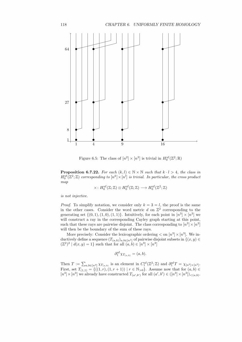
118 CHAPTER 6. UNIFORMLY FINITE HOMOLOGY
1 4 9 161
8
27
64
Figure 6.5: The class of [n2] × [n3] is trivial in Huf0 (Z2;R)
Proposition 6.7.22. For each (k, l) ∈ N × N such that k · l > 4, the class inHuf
0 (Z2;Z) corresponding to [nk]× [nl] is trivial. In particular, the cross productmap
× : Huf0 (Z;Z) ⊗Huf
0 (Z;Z) −→ Huf0 (Z2;Z)
is not injective.
Proof. To simplify notation, we consider only k = 3 = l, the proof is the samein the other cases. Consider the word metric d on Z2 corresponding to thegenerating set {(0, 1), (1, 0), (1, 1)}. Intuitively, for each point in [n3] × [n3] wewill construct a ray in the corresponding Cayley graph starting at this point,such that these rays are pairwise disjoint. The class corresponding to [n3]× [n3]will then be the boundary of the sum of these rays.
More precisely: Consider the lexicographic ordering < on [n3]× [n3]. We in-ductively define a sequence (T(a,b))a,b∈[n3] of pairwise disjoint subsets in {(x, y) ∈(Z2)2 | d(x, y) = 1} such that for all (a, b) ∈ [n3] × [n3]
∂uf1 χT(a,b)= (a, b).
Then T :=∑
a,b∈[n3] χT(a,b)is an element in Cuf
1 (Z2;Z) and ∂uf1 T = χ[n3]×[n3].
First, set T(1,1) = {((1, r), (1, r + 1)) | r ∈ N>0}. Assume now that for (a, b) ∈[n3]× [n3] we already have constructed T(a′,b′) for all (a′, b′) ∈ ([n3]× [n3])<(a,b).
6.7. DEGREE ZERO 119
Then we set
T(a,b) :={
(a+ s, b+ s), (a+ s+ 1, b+ s+ 1))∣∣ s ∈ {0, . . . , c(a,b) − 1}
}
∪(T(1,1) + (a+ c(a,b) − 1, b+ c(a,b) − 1)
)
where
c(a,b) := min{s ∈ N
∣∣∣ ((k + s, l + s), (k + s, l + s+ 1)) 6∈⋃
(a′,b′)∈[n3]×[n3]
(a′,b′)<(a,b)
T(a′,b′)
}.
So, roughly speaking, the T(a,b) are built by going diagonally up and to the rightuntil one finds a vacant vertical line and then going straight up, Figure 6.5.
By construction, for all (a, b) ∈ [n3] × [n3]
c(a,b) ≤ c(0,b).
Furthermore, for all s3 ∈ [n3] there are s2 many points of [n3] in the square{0, 1, . . . , s3} × {0, 1, . . . , s3}, i.e., we have |[n3] ∩ {0, 1, . . . , s3}2| = s2. Hence,since the rays are only going up and to the right:
c(0,s3) ≤ s2 < (s+ 1)3 − s3. (∗)
Now the vertical parts of the rays are disjoint by definition and the diagonalparts are disjoint because they are parallel for the same starting value of b anddisjoint for different starting values of b by (∗).

120 CHAPTER 6. UNIFORMLY FINITE HOMOLOGY

Appendix A
Strong Contractions
The core of Ivanov’s proof of the absolute mapping theorem [48, Theorem 4.1]is his construction of a norm non-increasing cochain contraction for the cochaincomplex B(Csing
∗ (X),R) for X a simply connected CW-complex. This has beenextended by Frigerio and Pagliantini [40] to a relative version for certain CW-pairs. In this section, we will recall the proofs of these results and extendthem to coefficients in V ′, where V can be an arbitrary Banach module. Asnoted by Buhler [22], it is not necessary to demand X to be countable when anappropriate version of the theorem of Dold and Thom is used, and we will alsomake use of this observation here.
Lemma A.1 ([48]). Let G be an Abelian topological group. For n ∈ N, theset Sn(G) of singular n-simplices is also an Abelian group. For each n ∈ N
and i ∈ {0, . . . , n}, let ℓ∞(∂Gi,n,R) : ℓ∞(Sn−1(G);R) −→ ℓ∞(Sn(G);R) be thedual of the i-th face map of Sn(G). Then there is a sequence (mn
R)n∈N of maps,
such that
(i) For each n ∈ N, the map mnR
: ℓ∞(Sn(G),R) −→ R is an Sn(G)-invariantmean.
(ii) For all n ∈ N>0 and i ∈ {0, . . . , n}
ℓ∞(∂Gi,n,R)∗mnR
= mn−1R
,
where ℓ∞(∂Gi,n,R)∗mnR
denotes the pull-back mean of mnR
under the face
map ℓ∞(∂Gi,n,R).
Proof. For each n ∈ N, the symmetric group Σn on n-letters acts on ∆n
by permutation of the coordinates, hence also on ℓ∞(Sn(G),R). We denoteby Mn ⊂ ℓ∞(Sn(G),R)′ the set of Σn-and Sn(G)-invariant means. Since Sn(G)is Abelian and thus amenable, there is an Sn(G)-invariant mean m on Sn(G),and we can find an Sn(G)- and Σn-invariant mean by setting
m′ :=1
n!·∑
σ∈Σn
σ ·m.
The set Mn is a weak-∗-closed subset of the unit ball of ℓ∞(Sn(G),R) and there-fore weak-∗-compact by the Banach-Alaoglu theorem. For any i ∈ {0, . . . , n},
121

122 APPENDIX A. STRONG CONTRACTIONS
the map ℓ∞(∂Gi,n,R) induces a weak-∗-continuous map fn : Mn −→ Mn−1. Foreach n ∈ N>0, i, j ∈ {0, . . . , n} and m ∈Mn, we have
ℓ∞(∂Gi,n,R)∗m = ℓ∞(∂Gj,n,R)∗m
by the Σn-invariance of m, thus fn does not depend on i and for all m ∈ Mn
and i ∈ {0, . . . , n}, we have ℓ∞(∂Gi,n,R)∗m = fn(m). Since the Mn are compactand non-empty, the limit of the directed system (f∗ : M∗ −→ M∗−1)∗∈N>0 isnon-empty. Any point in this limit is a sequence of means which satisfies thedesired properties.
Corollary A.2 ([54]). Let G be an Abelian topological group and V a Banachspace. Then there is a sequence (mn
V )n∈N of maps, such that
(i) For each n ∈ N, the map mnV : ℓ∞(Sn(G), V ′) −→ V ′ is an Sn(G)-equiva-
riant mean with coefficients in V ′, viewed as a trivial Sn(G)-module.
(ii) For all n ∈ N>0 and i ∈ {0, . . . , n}
ℓ∞(∂Gi,n, V′)∗mn
V = mn−1V .
Proof. Let (mnR
)n∈N be as in Lemma A.1. For all n ∈ N, set
mnV : ℓ∞(Sn(G), V ′) −→ V ′
ϕ 7−→(v 7−→ mn
R
(g 7−→ ϕ(g)(v)
)).
The first part follows directly from Lemma A.1 (i). For the second part, wehave for all n ∈ N, i ∈ {0, . . . , n} and all f ∈ ℓ∞(Sn−1(G), V ′)
ℓ∞(∂Gi,n, V′)∗mn
V (f) = mnV (f ◦ ∂Gi,n)
=(v 7−→ mn
R
(g 7−→ f(∂Gi,n(g))(v)
))
=(v 7−→ mn
R
(ℓ∞(∂Gi,n,R)
(g 7−→ f(g)(v)
)))
=(v 7−→ mn−1
R
(g 7−→ f(g)(v)
))
= mn−1V (f).
Proposition A.3 (Averaging cochains [48, 54]). Let G be an Abelian topologicalgroup and let p : X −→ Y be a principal G-bundle. Let V be Banach module.Then there is a cochain map
A∗ : B(Csing∗ (X), V ′) −→ B(Csing
∗ (Y ), V ′),
such that A∗ ◦B(Csing∗ (p), V ′) = idB(Csing
∗ (Y ),V ′) and ‖A∗‖∞ = 1.
Proof. The group Sn(G) acts on Sn(X) via pointwise multiplication, i.e.,
Sn(G) × Sn(X) −→ Sn(X)
(τ, σ) 7−→(t 7−→ τ(t) · σ(t)
).

123
For each σ ∈ Sn(Y ), write Fσ = {τ ∈ Sn(X) | p(τ) = σ}. For any lift σ of σ, wesee that Fσ is just the orbit Sn(G) · σ and since the action of Sn(G) on Sn(X)is free, there is an Sn(G)-isomorphism
ρσ : Sn(G) −→ Fσ
τ 7−→ τ · σ.
Let (mnV )n∈N be as in Corollary A.2. For each n ∈ N, set mn
σ = ℓ∞(ρσ, V′)∗mn
V .By the Sn(G)-invariance of mn
V , this does not depend on the choice of the lift σ.Now define for all n ∈ N
An : B(Csing∗ (X), V ′) −→ B(Csing
∗ (Y ), V ′)
f 7−→(σ 7−→ mn
σ(f |Fσ)).
Because each mnσ is a mean, we see for all n ∈ N that ‖An‖∞ ≤ 1 and
An ◦B(Csingn (p), V ′) = idB(Csing
n (Y ),V ′) .
Clearly, for any n ∈ N, any i ∈ {0, . . . , n}, any σ ∈ Sn(Y ) and any lift σ thefollowing diagram commutes, where the ∂?i,n are the corresponding i-th facemaps:
Fσ F∂Yi σ
Sn(G) Sn−1(G).
∂Xi,n|Fσ
ρσ
∂Gi,n
ρ∂Xi,nσ
Thus, Property (ii) from Corollary A.2 implies mn−1∂i,nσ = ℓ∞(∂Xi,n|Fσ
, V ′)∗mnσ.
Hence, A∗ is a cochain map, since for all n ∈ N>0, all i ∈ {0, . . . , n − 1},all f ∈ B(Cn−1(X), V ′) and all σ ∈ Sn(Y )
(δYi,n−1An−1(f))(σ) = An−1(f)(∂Yi,nσ)
= mn−1∂Yi,nσ
(f |F
∂Yi,n
σ
)
= mnσ
(ℓ∞(∂Xi,n|Fσ
, V ′)(f |F
∂Yi,n
σ
))
= mnσ
((δi,n−1
X f)|Fσ
)
= An(δi,n−1X f)(σ).
Theorem A.4 ([48]). Let X be a simply connected CW-complex. Then thereis a sequence
· · ·pn−→ Xn
pn−1−→ · · ·
p2−→ X2
p1−→ X1 := X,
such that for all n ∈ N>0:
(i) For all i ∈ {0, . . . , n}, we have πi(Xn) = 0.
(ii) For all i ∈ N>n, the map πi(pn) : πi(Xn+1) −→ πi(Xn) is an isomorphism.

124 APPENDIX A. STRONG CONTRACTIONS
(iii) The map pn : Xn+1 −→ Xn is a principal Gn-bundle, where Gn is a topo-logical Abelian group of type K(πn+1(X), n).
We call such a sequence a Dold-Thom-Whitehead tower for X .
Sketch of proof. Start with a Whitehead tower (X ′∗, p
′∗) [46, Example 4.20]. By
the theorem of Dold and Thom [32], or, when X is not countable, by its general-isation by McCord [56], we can find for each n ∈ N>0 a model of K(πn+1(X), n)which is a topological Abelian group. By a short argument comparing uni-versal bundles, one can show that one can replace the maps p′∗ by princi-pal K(πn+1(X), n)-bundles, [48, Lemma 2.3.3].
We recall the standard cone construction for highly connected spaces:
Remark A.5. For n ∈ N, let X be an n-connected topological space and x ∈ X .We want to define a family of maps (Lx
i : Si(X) −→ Si+1(X))i∈{0,...,n} such that
(i) For all y ∈ S0(X), we have ∂0,0Lx0(y) = y and ∂1,0L
x0(y) = x.
(ii) For all k ∈ {1, . . . , n} and all i ∈ {1, . . . , k}, we have
∂i,k+1 ◦ Lxk = Lx
k−1 ◦ ∂i−1,k
∂0,k+1 ◦ Lxk = idSk(X) .
We define the Lxk by induction on k. Since X is connected, we can find for
each y ∈ S0(X) ∼= X a path Lx0(y) from y to x, and Lx
0 satisfies (i). Assumethat L1, . . . , Lk have been defined for k ∈ {0, . . . , n − 1}. For each σ ∈ Sk(X)consider σ′ : ∂∆k+1 −→ X , such that for all i ∈ {1, . . . , k + 1}
σ′|∂i∆k+1 = Lkx(∂i−1∆k)
σ′|∂0∆k+1 = σ.
The map σ′ is well-defined by property (ii). Since X is k-connected, there isa k+1-simplex Lx
k(σ) ∈ Sk+1(X), such that Lxk(σ)|∂∆n+1 = σ′. By definition, Lx
k
has the desired properties.We call such a family Lx
∗ an n-partial coning contraction for X with respectto x.
If Lx∗ is such a coning contraction, the family
(txk : Csingk (X) −→ Csing
k+1(X))k∈{0,...,n},
induced by linearly extending Lx∗ , together with
tx−1 : R −→ Csing0 (X)
1 7−→ x
is an n-partial chain contraction, i.e., for all k ∈ {0, . . . , n}
∂k+1 ◦ txk + txk−1 ◦ ∂n = idCk(X)
and clearly ‖txk‖∞ ≤ 1 for all k ∈ {−1, . . . , n}.
The cone construction is not canonical, but sufficiently concrete to provefurther compatibility results:
125
Lemma A.6 ([48, 40]).
(i) Let X be a simply connected CW-complex. Let (X∗, p∗) be a Dold-Thom-Whitehead tower for X . Let (xn)n∈N>0 be a sequence of points, suchthat xn ∈ Xn and pn(xn+1) = xn for all n ∈ N>0. Then there existsa sequence (Lxn
∗ )n∈N>0 , such that Lxn∗ is an n-partial coning contraction
for Xn with respect to xn and for all n ∈ N>0 and k ∈ {0, . . . , n}
Sk+1(pn) ◦ Lxn+1
k = Lxn
k ◦ Sk(pn).
We call such a sequence (Lxn∗ )n∈N>0 a partial coning for the tower (X∗, p∗)
with respect to x1.
(ii) Let i : W −→ X be a CW-pair. Assume that W and X are simply con-nected and that i is a weak equivalence. Let (X∗, p∗) be a Dold-Thom-Whitehead tower. Set Wn := (p1 ◦ · · · ◦ pn)−1(W ). Then (W∗, p∗|W∗)is a Dold-Thom-Whitehead tower for W . Let in : Wn −→ Xn be thecanonical inclusion for each n ∈ N>0. For each a1 ∈ W , there exists apartial coning (Lan
∗ )n∈N>0 for (X∗, p∗) and a partial coning (Kan∗ )n∈N>0
for (W∗, p∗|W∗), such that for all n ∈ N
Sn+1(in+1) ◦Kann = Lan
n ◦ Sn(in).
Proof. The first part can be found in Ivanov’s article [48], the second one in thearticle of Frigerio and Pagliantini [40].
Theorem A.7 ([48, 54]). Let X be a simply connected CW-complex and Va Banach module. Then for each x ∈ X there is a strong pointed cochaincontraction
(s∗x : B(Csing∗ (X ;R), V ′) −→ B(Csing
∗−1(X ;R), V ′))∗∈N
Proof. We follow Ivanov’s proof [48], but with coefficients in V ′. Let (Lxn∗ )n∈N>0
be a partial coning for the Dold-Thom-Whitehead tower (X∗, p∗) for X1 = Xwith respect to x1 = x as in Lemma A.6 (i). For each n ∈ N let
(tkn : B(Csingk (Xn), V ′) −→ B(Csing
k−1(Xn), V ′))k∈{1,...,n+1}
be as in Remark A.5. For each n ∈ N>0, consider
A∗n : B(Csing
∗ (Xn), V ′) −→ B(Csing∗ (Xn−1), V ′)
as in Proposition A.3. For each n ∈ N, set p∗n := B(Csing∗ (pn), V ′) and define
(s∗x : B(Csing∗ (X), V ′) −→ B(Csing
∗−1(X), V ′))∗∈N
by setting for all n ∈ N>0
snx := An−12 ◦ · · · ◦An−1
n+1 ◦ tnn+1 ◦ p
nn ◦ · · · ◦ pn1

126 APPENDIX A. STRONG CONTRACTIONS
Then ‖snx‖∞ ≤ 1, since this holds also for all An∗ , p
n∗ and tnn. Since for all n ∈ N
δn−1 ◦ snx + sn+1x ◦ δn
= δn−1 ◦An−12 ◦ · · · ◦An−1
n+1 ◦ tnn+1 ◦ p
nn ◦ · · · ◦ pn1
+An2 ◦ · · · ◦An
n+2 ◦ tn+1n+2 ◦ p
n+1n+1 ◦ · · · ◦ p
n+11 ◦ δn
= An2 ◦ · · · ◦An
n+1 ◦(δn−1 ◦ tnn+1 +An
n+2 ◦ tn+1n+2 ◦ p
n+1n+1 ◦ δ
n)◦ pnn ◦ · · · ◦ pn1
= An2 ◦ · · · ◦An
n+1 ◦(δn−1 ◦ tnn+1 +An
n+2 ◦ pnn+1 ◦ t
n+1n+1 ◦ δ
n)◦ pnn ◦ · · · ◦ pn1
= An2 ◦ · · · ◦An
n+1 ◦(δn−1 ◦ tnn+1 + tn+1
n+1 ◦ δn)◦ pnn ◦ · · · ◦ pn1
= An2 ◦ · · · ◦An
n+1 ◦ pnn ◦ · · · ◦ pn1
= idB(Cn(X),V ′),
the family s∗x is a cochain contraction.
Proposition A.8 ([40]). Let i : A −→ X be a pair of connected CW-comp-lexes, such that i is π1-injective and induces an isomorphism between the higherhomotopy groups. Let V be a Banach module. Let i : A −→ X be a fixed inclu-sion map. Then there exists a family of norm non-increasing, pointed cochaincontractions
((s∗x : B(Csing
∗ (X), V ′) −→ B(Csing∗−1(X;R), V ′)
)∗∈N>0
s0x : B(Csing0 (X ;R), V ′) −→ V ′
)
x∈X
and a family of norm non-increasing, pointed cochain contractions
((s∗a : B(Csing
∗ (A;R), V ′) −→ B(Csing∗−1(A;R), V ′)
)∗∈N>0
s0a : B(Csing0 (A;R), V ′) −→ V ′
)
a∈A
that is compatible with the restriction to A, i.e., the following diagram commutesfor all a ∈ A:
B(Csing∗ (X), V ′) B(Csing
∗−1(X), V ′)
B(Csing∗ (A), V ′) B(Csing
∗−1(A), V ′)
s∗i(a)
B(Csing∗ (i), V ′)
s∗a
B(Csing∗−1 (i), V ′)
Proof. The proof is the same as the one of Theorem A.7, applied to the com-patible partial conings from Lemma A.6 (ii).
Remark A.9. The condition on the higher homotopy groups is needed in orderto have compatible Dold-Thom-Whitehead towers for the pair (X,A), since un-der this condition one can use the same averaging constructions in the definitionof both cochain contractions. If the condition on the higher homotopy groupsis not satisfied, one could try to use a functorial version of the Whitehead tow-ers, but then the relation between the averaging maps is completely unclear. Ifone tries instead to use the preimages An := (p1 ◦ · · · pn)−1(A) of A inside the

127
Whitehead tower over X , one has compatible averaging maps, but as noted byPagliantini [66, Remark 2.29] in general it is impossible to use a relative coneconstruction with respect to the pair (Xn, An), since the homotopy groups of An
will be in general non-trivial.

128 APPENDIX A. STRONG CONTRACTIONS

Bibliography
[1] C. Anantharaman and J. Renault. Amenable groupoids. In Groupoidsin analysis, geometry, and physics (Boulder, CO, 1999), volume 282 ofContemp. Math., pages 35–46. Amer. Math. Soc., Providence, RI, 2001.
[2] C. Anantharaman-Delaroche and J. Renault. Amenable groupoids,volume 36 of Monographies de L’Enseignement Mathematique.L’Enseignement Mathematique, Geneva, 2000. With a foreword byGeorges Skandalis and Appendix B by E. Germain.
[3] M. Aschenbrenner, S. Friedl, and H. Wilton. 3-manifold groups. ArXive-prints:1205.0202, May 2012.
[4] G. Baumslag, C. Miller, and H. Short. Isoperimetric inequalities and thehomology of groups. Invent. Math., 113(3):531–560, 1993.
[5] C. Bavard. Longueur stable des commutateurs. Enseign. Math. (2), 37(1-2):109–150, 1991.
[6] I. Belegradek. Aspherical manifolds with relatively hyperbolic fundamentalgroups. Geom. Dedicata, 129:119–144, 2007.
[7] R. Benedetti and C. Petronio. Lectures on hyperbolic geometry. Universi-text. Springer-Verlag, Berlin, 1992.
[8] M. Bestvina and K. Fujiwara. Bounded cohomology of subgroups of map-ping class groups. Geom. Topol., 6:69–89 (electronic), 2002.
[9] M. Blank and F. Diana. Uniformly finite homology and amenable groups.ArXiv e-prints:1309.6097, September 2013. To appear in Algebraic & Ge-ometric Topology.
[10] J. Block and S. Weinberger. Aperiodic tilings, positive scalar curvatureand amenability of spaces. J. Amer. Math. Soc., 5(4):907–918, 1992.
[11] M. R. Bridson and A. Haefliger. Metric spaces of non-positive curvature,volume 319 of Grundlehren der Mathematischen Wissenschaften. Springer-Verlag, Berlin, 1999.
[12] J. Brodzki, G. A. Niblo, and N. Wright. Pairings, duality, amenability andbounded cohomology. J. Eur. Math. Soc. (JEMS), 14(5):1513–1518, 2012.
129

130 BIBLIOGRAPHY
[13] R. Brooks. Some remarks on bounded cohomology. In Riemann surfacesand related topics: Proceedings of the 1978 Stony Brook Conference (StateUniv. New York, Stony Brook, N.Y., 1978), volume 97 of Ann. of Math.Stud., pages 53–63. Princeton Univ. Press, Princeton, N.J., 1981.
[14] R. Brooks and C. Series. Bounded cohomology for surface groups. Topology,23(1):29–36, 1984.
[15] K. S. Brown. Cohomology of groups, volume 87 of Graduate Texts in Math-ematics. Springer-Verlag, New York-Berlin, 1982.
[16] R. Brown. Topology and groupoids. BookSurge, LLC, Charleston, SC, 2006.Third edition of Elements of modern topology.
[17] M. Bucher. Simplicial volume of products and fiber bundles. In Discretegroups and geometric structures, volume 501 of Contemp. Math., pages79–86. Amer. Math. Soc., Providence, RI, 2009.
[18] M. Bucher, M. Burger, R. Frigerio, A. Iozzi, C. Pagliantini, and M. B.Pozzetti. Isometric embeddings in bounded cohomology. ArXiv e-prints:1305.2612, May 2013.
[19] M. Bucher, M. Burger, and A. Iozzi. A dual interpretation of the Gromov-Thurston proof of Mostow rigidity and volume rigidity for representationsof hyperbolic lattices. In Trends in harmonic analysis, volume 3 of SpringerINdAM Ser., pages 47–76. Springer, Milan, 2013.
[20] M Bucher-Karlsson. The proportionality constant for the simplicial volumeof locally symmetric spaces. Colloq. Math., 111(2):183–198, 2008.
[21] M. Bucher-Karlsson. The simplicial volume of closed manifolds covered byH2 ×H2. J. Topol., 1(3):584–602, 2008.
[22] T. Buhler. On the algebraic foundations of bounded cohomology. Mem.Amer. Math. Soc., 214(1006):xxii+97, 2011.
[23] M. Burger and A. Iozzi. Bounded differential forms, generalized Milnor-Wood inequality and an application to deformation rigidity. Geom. Dedi-cata, 125:1–23, 2007.
[24] M. Burger and N. Monod. Bounded cohomology of lattices in higher rankLie groups. J. Eur. Math. Soc. (JEMS), 1(2):199–235, 1999.
[25] D. Calegari. scl, volume 20 of MSJ Memoirs. Mathematical Society ofJapan, Tokyo, 2009.
[26] T. Ceccherini-Silberstein and M. Coornaert. Cellular automata and groups.Springer Verlag, 2010. Springer Monographs in Mathematics.
[27] I. Chatterji, T. Fernos, and A. Iozzi. The median class and superrigidityof actions on cat(0) cube complexes. ArXiv e-prints:1212.1585, December2014.
[28] C. Chou. The exact cardinality of the set of invariant means on a group.Proc. Amer. Math. Soc., 55(1):103–106, 1976.

BIBLIOGRAPHY 131
[29] M. W. Davis, T. Januszkiewicz, and S. Weinberger. Relative hyper-bolization and aspherical bordisms: an addendum to “Hyperbolization ofpolyhedra” [J. Differential Geom. 34 (1991), no. 2, 347–388; MR1131435(92h:57036)] by Davis and Januszkiewicz. J. Differential Geom., 58(3):535–541, 2001.
[30] F. Diana. Aspects of uniformly finite homology. PhD thesis, UniversitatRegensburg, 2014.
[31] F. Diana and P. W. Nowak. Eilenberg swindles and higher large scalehomology of products. ArXiv e-prints:1409.5219, September 2014.
[32] A. Dold and R. Thom. Quasifaserungen und unendliche symmetrischeProdukte. Ann. of Math. (2), 67:239–281, 1958.
[33] A. Dranishnikov. Macroscopic dimension and essential manifolds. Tr. Mat.Inst. Steklova, 273(Sovremennye Problemy Matematiki):41–53, 2011.
[34] A. Dranishnikov. On macroscopic dimension of rationally essential mani-folds. Geom. Topol., 15(2):1107–1124, 2011.
[35] A. Dranishnikov. On macroscopic dimension of universal coverings of closedmanifolds. Trans. Moscow Math. Soc., pages 229–244, 2013.
[36] T. Dymarz. Bilipschitz equivalence is not equivalent to quasi-isometricequivalence for finitely generated groups. Duke Math. J., 154(3):509–526,2010.
[37] D. Epstein and K. Fujiwara. The second bounded cohomology of word-hyperbolic groups. Topology, 36(6):1275–1289, 1997.
[38] B. Evans and L. Moser. Solvable fundamental groups of compact 3-manifolds. Trans. Amer. Math. Soc., 168:189–210, 1972.
[39] R. Frigerio. (Bounded) continuous cohomology and Gromov’s proportion-ality principle. Manuscripta Math., 134(3-4):435–474, 2011.
[40] R. Frigerio and C. Pagliantini. Relative measure homology and continuousbounded cohomology of topological pairs. Pacific J. Math., 257(1):91–130,2012.
[41] K. Fujiwara and K. Ohshika. The second bounded cohomology of 3-manifolds. Publ. Res. Inst. Math. Sci., 38(2):347–354, 2002.
[42] S. M. Gersten. Bounded cocycles and combings of groups. Internat. J.Algebra Comput., 2(3):307–326, 1992.
[43] S. M. Gersten. A cohomological characterization of hyperbolic groups. Un-published, available online via www.math.utah.edu/~sg/Papers/ch.pdf,1996.
[44] S. M. Gersten. Cohomological lower bounds for isoperimetric functions ongroups. Topology, 37(5):1031–1072, 1998.
[45] M. Gromov. Volume and bounded cohomology. Inst. Hautes Etudes Sci.Publ. Math., (56):5–99 (1983), 1982.

132 BIBLIOGRAPHY
[46] A. Hatcher. Algebraic topology. Cambridge University Press, Cambridge,2002.
[47] P. J. Hilton and U. Stammbach. A course in homological algebra, volume 4of Graduate Texts in Mathematics. Springer-Verlag, New York, secondedition edition, 1997.
[48] N. V. Ivanov. Foundations of the theory of bounded cohomology. Zap.Nauchn. Sem. Leningrad. Otdel. Mat. Inst. Steklov. (LOMI), 143:69–109,177–178, 1985. Studies in topology, V.
[49] B. E. Johnson. Cohomology in Banach algebras. American MathematicalSociety, Providence, R.I., 1972. Memoirs of the American MathematicalSociety, No. 127.
[50] J. Kelley and I. Namioka. Linear topological spaces. Springer-Verlag, NewYork-Heidelberg, 1976. Second corrected printing, Graduate Texts in Math-ematics, No. 36.
[51] S. Kim and T. Kuessner. Simplicial volume of compact manifolds withamenable boundary. ArXiv e-prints:1205.1375, May 2012.
[52] B. Kleiner and B. Leeb. Groups quasi-isometric to symmetric spaces.Comm. Anal. Geom., 9(2):239–260, 2001.
[53] C. Loh. Measure homology and singular homology are isometrically iso-morphic. Math. Z., 253(1):197–218, 2006.
[54] C. Loh. ℓ1-Homology and Simplicial Volume. PhD thesis, Univer-sitat Munster, 2007. http://nbn-resolving.de/urn:nbn:de:hbz:
6-37549578216.
[55] J. P. May. Simplicial objects in algebraic topology. Chicago Lectures inMathematics. University of Chicago Press, Chicago, IL, 1992. Reprint ofthe 1967 original.
[56] M. C. McCord. Classifying spaces and infinite symmetric products. Trans.Amer. Math. Soc., 146:273–298, 1969.
[57] I. Mineyev. Higher dimensional isoperimetric functions in hyperbolicgroups. Math. Z., 233(2):327–345, 2000.
[58] I. Mineyev. Straightening and bounded cohomology of hyperbolic groups.Geom. Funct. Anal., 11(4):807–839, 2001.
[59] I. Mineyev. Bounded cohomology characterizes hyperbolic groups. Q. J.Math., 53(1):59–73, 2002.
[60] I. Mineyev, N. Monod, and Y. Shalom. Ideal bicombings for hyperbolicgroups and applications. Topology, 43(6):1319–1344, 2004.
[61] I. Mineyev and A. Yaman. Relative hyperbolicity and bounded cohomol-ogy. Unpublished, available online via www.math.uiuc.edu/~mineyev/
math/art/rel-hyp.pdf, 2006.

BIBLIOGRAPHY 133
[62] N. Monod. Continuous bounded cohomology of locally compact groups, vol-ume 1758 of Lecture Notes in Mathematics. Springer-Verlag, Berlin, 2001.
[63] N. Monod and Y. Shalom. Cocycle superrigidity and bounded cohomologyfor negatively curved spaces. J. Differential Geom., 67(3):395–455, 2004.
[64] H. J. Munkholm. Simplices of maximal volume in hyperbolic space, Gro-mov’s norm, and Gromov’s proof of Mostow’s rigidity theorem (followingThurston). In Topology Symposium, Siegen 1979 (Proc. Sympos., Univ.Siegen, Siegen, 1979), volume 788 of Lecture Notes in Math., pages 109–124. Springer, Berlin, 1980.
[65] G. A. Noskov. Bounded cohomology of discrete groups with coefficients (inrussian). Algebra i Analiz, 2(5):146–164, 1990.
[66] C. Pagliantini. Relative (continuous) bounded cohomology and simplicialvolume of hyperbolic manifolds with geodesic boundary. PhD thesis, Univer-sita di Pisa, 2012. http://etd.adm.unipi.it/t/etd-07112012-101103/.
[67] C. D. Papakyriakopoulos. On Dehn’s lemma and the asphericity of knots.Ann. of Math. (2), 66:1–26, 1957.
[68] H. Park. Relative bounded cohomology. Topology Appl., 131(3):203–234,2003.
[69] A. Paterson. Amenability, volume 29 of Mathematical Surveys and Mono-graphs. American Mathematical Society, Providence, RI, 1988.
[70] P. Scott. The geometries of 3-manifolds. Bull. London Math. Soc.,15(5):401–487, 1983.
[71] C. Series. An application of groupoid cohomology. Pacific J. Math.,92(2):415–432, 1981.
[72] T. Soma. The Gromov invariant of links. Invent. Math., 64(3):445–454,1981.
[73] U. Stammbach. On the weak homological dimension of the group algebraof solvable groups. J. London Math. Soc. (2), 2:567–570, 1970.
[74] W. Thurston. The geometry and topology of 3-manifolds. Lecture notes,Princeton. Available online via http://library.msri.org/books/gt3m/,1978-80.
[75] J. Tu. Groupoid cohomology and extensions. Trans. Amer. Math. Soc.,358(11):4721–4747 (electronic), 2006.
[76] C. A. Weibel. An introduction to homological algebra, volume 38 of Cam-bridge Studies in Advanced Mathematics. Cambridge University Press,Cambridge, 1994.
[77] J. H. C. Whitehead. On 2-spheres in 3-manifolds. Bull. Amer. Math. Soc.,64:161–166, 1958.
[78] K. Whyte. Amenability, bi-Lipschitz equivalence, and the von Neumannconjecture. Duke Math. J., 99(1):93–112, 1999.