Relativistic Hamiltonian Dynamics in Nuclear and … · Relativistic Hamiltonian Dynamics in Nuclear and ... conclusion for systems of interacting particles. ... interactions in relativistic

Relativistic Hamiltonian Dynamics in Nuclear and Particle Physics

B. D. Keister

Physics Department

Carnegie Mellon University

Pittsburgh, PA 15213

and

W. N. Polyzou

Department of Physics and Astronomy

The University of Iowa

Iowa City, IA 52242

ABSTRACT

This review is intended to provide an introduction to the formulation of rel-

ativistic quantum mechanical models, particularly for use in strong interaction

problems, whose dynamics is given by a unitary representation of the inhomo-

geneous Lorentz group. In the first portion, an overview is given in which the

properties of these models are defined and some analytically solvable examples are

given. This is followed by a deductive construction of these models from physical

principles. Particle production, electron scattering, macroscopic locality, and the

relation to local quantum field theory are discussed in the second half.

RELATIVISTIC HAMILTONIAN DYNAMICS IN

NUCLEAR AND PARTICLE PHYSICS

B. D. Keister and W. N. Polyzou

To be published in:

ADVANCES IN NUCLEAR PHYSICS

Ed. J. W. Negele and Erich Vogt

Plenum Press • New York-London

RELATIVISTIC HAMILTONIAN DYNAMICS IN

NUCLEAR AND PARTICLE PHYSICS

B. D. Keister and W. N. Polyzou

CONTENTS

1. Introduction . . . . . . . . . . . . . . . . . . . . . . . . . . . . . . . . 1

2. Relativistic Quantum Mechanics: Principles and Examples . . . . . . . . . . . . 8

2.1 Relativistic Invariance . . . . . . . . . . . . . . . . . . . . . . . . . . . 8

2.2 Historical Perspective . . . . . . . . . . . . . . . . . . . . . . . . . . 11

2.3 Confined Spinless Quarks . . . . . . . . . . . . . . . . . . . . . . . . 26

2.4 Confined Relativistic Quarks - With Spin . . . . . . . . . . . . . . . . . 39

2.5 Spinless Two Particle Scattering . . . . . . . . . . . . . . . . . . . . . 45

2.6 Nucleon-Nucleon Scattering - With Spin . . . . . . . . . . . . . . . . . . 61

2.7 Summary of Examples . . . . . . . . . . . . . . . . . . . . . . . . . . 70

3. Symmetries in Quantum Mechanics . . . . . . . . . . . . . . . . . . . . . 71

3.1 Galilean Relativity . . . . . . . . . . . . . . . . . . . . . . . . . . . 74

3.2 Special Relativity - The Poincare Group . . . . . . . . . . . . . . . . . . 79

3.3 Parameterization of Poincare Transformations . . . . . . . . . . . . . . . 81

3.4 Definition of Infinitesimal Generators . . . . . . . . . . . . . . . . . . . 82

3.5 Commutation Relations - Canonical Form . . . . . . . . . . . . . . . . . 82

3.5.1 Commutation Relations - Covariant Form . . . . . . . . . . . . . . . 84

3.5.2 Commutation Relations - Front Form . . . . . . . . . . . . . . . . . 85

3.6 Commuting Self Adjoint Operators . . . . . . . . . . . . . . . . . . . . 86

3.6.1 The Mass Operator . . . . . . . . . . . . . . . . . . . . . . . . . 86

3.6.2 The Pauli-Lubanski Operator . . . . . . . . . . . . . . . . . . . . . 87

3.6.3 Boosts . . . . . . . . . . . . . . . . . . . . . . . . . . . . . . . 88

3.6.4 Spin Vectors . . . . . . . . . . . . . . . . . . . . . . . . . . . . 90

3.7 Other Considerations . . . . . . . . . . . . . . . . . . . . . . . . . . 93

4. The One-Body Problem - Irreducible Representations . . . . . . . . . . . . . 95

4.1 The Hilbert Space . . . . . . . . . . . . . . . . . . . . . . . . . . . . 95

4.2 Unitary Representations . . . . . . . . . . . . . . . . . . . . . . . . . 98

4.3 Lie Algebra . . . . . . . . . . . . . . . . . . . . . . . . . . . . . . 104

4.4 Position in Relativity . . . . . . . . . . . . . . . . . . . . . . . . . . 108

4.5 Summary . . . . . . . . . . . . . . . . . . . . . . . . . . . . . . . 110

5. The Two-Body Problem . . . . . . . . . . . . . . . . . . . . . . . . . . 112

5.1 The Two-Body Hilbert Space . . . . . . . . . . . . . . . . . . . . . . . 113

5.2 Relativistic Dynamics of Two Free Particles . . . . . . . . . . . . . . . . 113

5.3 Clebsch-Gordan Coefficients . . . . . . . . . . . . . . . . . . . . . . . 114

5.4 Free-Particle Generators and Other Operators . . . . . . . . . . . . . . . 121

5.5 The Bakamjian-Thomas Construction . . . . . . . . . . . . . . . . . . . 123

5.6 Special Cases . . . . . . . . . . . . . . . . . . . . . . . . . . . . . . 129

5.6.1 The Instant Form . . . . . . . . . . . . . . . . . . . . . . . . . . 130

5.6.2 The Front Form . . . . . . . . . . . . . . . . . . . . . . . . . . . 132

5.6.3 The Point Form . . . . . . . . . . . . . . . . . . . . . . . . . . . 134

6. The 2+1 Body Problem . . . . . . . . . . . . . . . . . . . . . . . . . . 137

6.1 Macroscopic Locality and the 2+1 Body Problem . . . . . . . . . . . . . . 137

6.2 The Three-Body Hilbert Space . . . . . . . . . . . . . . . . . . . . . . 142

6.3 Two 2+1 Body Models . . . . . . . . . . . . . . . . . . . . . . . . . 145

6.4 Packing Operators . . . . . . . . . . . . . . . . . . . . . . . . . . . 151

7. The Three-Body Problem . . . . . . . . . . . . . . . . . . . . . . . . . . 157

7.1 Three-Body Constructions . . . . . . . . . . . . . . . . . . . . . . . . 157

7.1.1 Poincare Invariance in the Three-Body Problem . . . . . . . . . . . . . 157

7.1.2 Bakamjian-Thomas Construction . . . . . . . . . . . . . . . . . . . 161

7.1.3 Packing Operators . . . . . . . . . . . . . . . . . . . . . . . . . . 163

7.2 Faddeev Equations . . . . . . . . . . . . . . . . . . . . . . . . . . . 172

7.3 Symmetric Coupling Schemes . . . . . . . . . . . . . . . . . . . . . . . 180

7.4 Remarks . . . . . . . . . . . . . . . . . . . . . . . . . . . . . . . . 187

8. Particle Production . . . . . . . . . . . . . . . . . . . . . . . . . . . . 189

8.1 The Hilbert Space . . . . . . . . . . . . . . . . . . . . . . . . . . . . 191

8.2 Free-Particle Dynamics . . . . . . . . . . . . . . . . . . . . . . . . . . 193

8.3 Interactions . . . . . . . . . . . . . . . . . . . . . . . . . . . . . . 196

8.4 Macroscopic Locality . . . . . . . . . . . . . . . . . . . . . . . . . . 200

9. Electromagnetic Currents and Tensor Operators . . . . . . . . . . . . . . . . 205

9.1 Basic Formulas and Observables . . . . . . . . . . . . . . . . . . . . . . 206

9.2 Matrix Elements and Invariants . . . . . . . . . . . . . . . . . . . . . . 212

9.2.1 Matrix Elements of Tensor Operators . . . . . . . . . . . . . . . . . 213

9.2.2 Front-Form Matrix Elements . . . . . . . . . . . . . . . . . . . . . 221

9.2.3 Example: Matrix Elements of Field Operators . . . . . . . . . . . . . . 221

9.2.4 Four-Vector Current Matrix Elements . . . . . . . . . . . . . . . . . . 222

9.2.5 Symmetries and Constraints . . . . . . . . . . . . . . . . . . . . . . 224

9.2.6 Front-Form Current Matrix Elements . . . . . . . . . . . . . . . . . 225

9.2.7 Example: The π → ρ Transition Form Factor . . . . . . . . . . . . . . 228

9.3 Computation of Composite Form Factors . . . . . . . . . . . . . . . . . . 230

9.3.1 Basic Requirements of Current Operators . . . . . . . . . . . . . . . . 230

9.3.2 Impulse Approximation . . . . . . . . . . . . . . . . . . . . . . . 235

9.3.3 Example: The π → ρ Transition Form Factor . . . . . . . . . . . . . . 238

10. Relation To Covariant Theories . . . . . . . . . . . . . . . . . . . . . . . 241

11. Conclusion . . . . . . . . . . . . . . . . . . . . . . . . . . . . . . . . 254

Acknowledgements . . . . . . . . . . . . . . . . . . . . . . . . . . . . . . 257

Appendix A: Scattering Theory . . . . . . . . . . . . . . . . . . . . . . . . 258

A.1 The Relation Between S and T . . . . . . . . . . . . . . . . . . . . . . 258

A.2 The Invariance Principle . . . . . . . . . . . . . . . . . . . . . . . . . 262

A.3 Cross Sections . . . . . . . . . . . . . . . . . . . . . . . . . . . . . 265

A.4 Phenomenological Interactions . . . . . . . . . . . . . . . . . . . . . . 271

Appendix B: Front Form Kinematics . . . . . . . . . . . . . . . . . . . . . . 275

Appendix C: Racah Coefficients . . . . . . . . . . . . . . . . . . . . . . . . 281

Appendix D: Local Fields . . . . . . . . . . . . . . . . . . . . . . . . . . . 284

D.1 Fixed Number of Particles - Galilean Invariance: . . . . . . . . . . . . . . 285

D.2 Fixed Number of Particles - Poincare Invariance: . . . . . . . . . . . . . . 287

D.3 Fields . . . . . . . . . . . . . . . . . . . . . . . . . . . . . . . . . 292

D.1.1 Quasilocal Fields . . . . . . . . . . . . . . . . . . . . . . . . . . 294

D.4 The One-Body Subspace . . . . . . . . . . . . . . . . . . . . . . . . . 298

D.5 The Two-Body Subspace/Interactions . . . . . . . . . . . . . . . . . . . 303

References . . . . . . . . . . . . . . . . . . . . . . . . . . . . . . . . . . 311

Index . . . . . . . . . . . . . . . . . . . . . . . . . . . . . . . . . . . . 320

1. Introduction

Strong-interaction problems in nuclear and particle physics are often formulated in terms

of phenomenological models because of the difficulties in formulating convergent approximations

in local field theories such as QCD. Phenomenological models are designed to be simple enough

that they can be solved accurately and, if they are suitably refined, they can lead to realistic

descriptions of physical systems, as is the case in atomic and molecular physics and low energy

nuclear physics. For many problems of current interest in nuclear physics these models must be

consistent with the principle of special relativity. Relativity is needed to model reactions where

particles are produced, reactions involving energy and momentum transfers that are comparable

to the mass scales of the problem, bound systems where the binding energies are comparable

to the masses of the constituent particles, and coordinate system independent treatments of

problems in lepton-hadron scattering.

Relativistic quantum mechanics began with attempts to construct manifestly covariant ex-

tensions of the Schrodinger equation. Schrodinger (Sc 26) had already discovered and discarded

the Klein-Gordon equation (Kl 26, Go 26a, Go 26b) in his original paper. It was realized early on

by Heisenberg, Born and Jordan (Bo 26) that laws of quantum mechanics also should apply to

the electromagnetic field, which transforms covariantly under Poincare transformations. This led

to the introduction of the quantum theory of the electromagnetic field (Di 27, He 29, Sc 58). The

impressive agreement of the predictions of quantum electrodynamics with experiment, coupled

with the realization that a quantized field provided a means for avoiding the concept of instan-

taneous action at a distance, led to the acceptance of local relativistic field theory as the correct

way to model the fundamental interactions of nature at accessible energies.

For the strong interaction, however, ab initio calculations based on local field theories are

difficult because the infinite number of degrees of freedom and the large coupling constants make

it difficult to control the size of the error in any calculation. Field theoretic calculations involve

manipulations of a finite number of renormalized Feynman diagrams, using ladder sums (Sa 51)

or other techniques. These calculations ignore an infinite number of graphs with large coupling

constants and they fail to address the extent to which the terms in the perturbation series define

1

the dynamics. In addition, most applications in nuclear physics involve composite systems, either

of nuclei composed of nucleons, or of nucleons composed of quarks and gluons. The treatment

of composite systems in quantum field theories is nonperturbative at the outset. For the case of

nucleons as composites of quarks and gluons, the problem is more difficult because the quark and

gluon fields do not correspond to observable particles. At present there are no known algorithms

for constructing approximate solutions of dynamical problems in strongly interacting quantum

field theories with arbitrary precision.

Integral formulations of field theory, such as lattice approximations, (Wi 74) may ultimately

lead to computational methods where errors can be controlled. These methods are not developed

to the point where they provide sufficient control of computational error to make many useful

quantitative statements about nuclear or hadronic dynamics of realistic systems.

In spite of the acceptance of field theories as a matter of principle, most realistic dynam-

ical calculations in nuclear physics, and many in particle physics, utilize the nonrelativistic

Schrodinger equation. Nonrelativistic models can be solved using well defined computational

algorithms (Fa 65, Ya 67) in which errors can be made as small as desired. In a nonrelativistic

approach, one begins with a large class of models, most of which can be discarded upon compari-

son with experiment. In a field theoretic approach, one begins with a smaller class of models, but

in most cases, it is impossible to perform a calculation with errors small enough to discard the

model if it is not in agreement with experiment. Although the problem of putting error bounds

on field theoretic calculations can be justifiably considered a technical problem, it has resisted

solution for over 50 years.

Subsequent to the development of quantum field theory, Wigner (Wi 39) analyzed the math-

ematical formulation of the physical requirement of special relativity in quantum mechanics.

Physical states in quantum mechanics are in one-to-one correspondence with one-dimensional

subspaces, or “rays,” of the Hilbert space. Wigner showed that a necessary and sufficient condi-

tion for quantum mechanical probabilities to have values that are independent of the choice of

inertial coordinate system is the existence of a unitary ray representation of the inhomogeneous

Lorentz group (Poincare group) on the quantum mechanical Hilbert space. Wigner’s analysis ap-

plies both to quantum field theories and to quantum theories of particles, although its application

2

to theories of particles was not vigorously pursued at the time.

Most of what follows in this review is motivated by five seminal papers that took the work

of Wigner to its logical conclusion for systems of interacting particles. First, Dirac (Di 49)

formulated the problem of including interactions in relativistic classical mechanics. This was

done in Hamiltonian form, which has a natural canonical quantization. Although Dirac did

not solve the classical problem, he simplified it to one of several simpler problems. These three

different types of solutions to this problem are now called the “point,” “instant” and “front” forms

of the dynamics. Bakamjian and Thomas (Ba 53) successfully constructed the first relativistic

quantum mechanical model of two interacting particles in Dirac’s “instant” form of dynamics.

Foldy (Fo 61) recognized the importance of macroscopic locality as an additional constraint on

these models. This condition replaces the concept of Einstein causality or microscopic locality in

local field theories. Coester (Co 65) then extended the work of Bakamjian and Thomas to systems

of three particles, with a scattering operator consistent with the principle of macroscopic locality.

Finally, Sokolov (So 77) provided the general construction for N particles in a manner consistent

with macroscopic locality. These five papers define the scope of this review. Relativistic quantum

mechanical models of directly interacting particles have the following features:

• consistency with requirements of relativity and quantum mechanics

• connection between few-body dynamics and the many-body problem

• possibility of composite particles

• large class of permissible interactions

• tractable few-body calculation

We believe that such models are very attractive for a wide variety of applications in nuclear and

particle physics.

Relativistic direct interaction theories of particles lie between local field theoretic models

and nonrelativistic quantum mechanical models. They are applicable to situations involving

larger momentum transfers and binding energies than nonrelativistic models, and they permit

the formulation of invariant calculations involving particle production, electromagnetic and weak

probes (in the one-boson exchange approximation); none of the latter applications is possible

3

in nonrelativistic models. They replace the microscopic locality of field theories with a weaker

condition, called macroscopic locality, but, unlike field theories, lead to mathematically well

defined models where computational error can be controlled. Because of this, they should provide

a useful framework for the construction of mathematical models of the dynamics of hadrons and

nuclei at intermediate energies.

In comparing the contents of this review to other formulations of relativistic quantum me-

chanics, it is useful to keep in mind that there are (at least) two ways to consider the formulation

of this problem. The most common is to begin with a local relativistic field theory, and trun-

cate the dynamics in such a way that what remains is a closed system of dynamical equations

involving a finite number of important degrees of freedom. A second approach is to assume that

the system is governed by a finite number of degrees of freedom, and then to construct the most

general class of dynamical models with these degrees of freedom, consistent with a set of general

principles that include relativistic invariance. In some cases, equations obtained by these two

different approaches may be identical, but the emphasis and subsequent application is usually

different.

In the first approach, the connection to field theory is emphasized. In general, relations such

as the Schwinger-Dyson equations involve an infinite number of coupled amplitudes. Models

are constructed by retaining the coupling only among a finite number of amplitudes, or by

replacing an unknown amplitude with a phenomenological amplitude. Ladder approximations to

the Bethe-Salpeter equation (Sa 51) and approaches based upon mean field theory (Se 86) are

typical examples. We refer to these procedures as truncations. In general, truncations are not

controlled approximations, and the physical properties of the field theory (i.e., the axioms of field

theory) are not necessarily preserved on truncation. The models may violate Poincare invariance,

current covariance, or other symmetries; one must then believe that for a sensible truncation, the

corrections needed to restore these symmetries are small.

In the second approach, basic principles are emphasized. The connection to field theory

is of secondary concern. In this case, some principles have to be given up in passing from

a local field theory to a particle theory, but this is accomplished directly by weakening specific

axioms. In this paper the axiom of microscopic locality is replaced by a weaker requirement called

4

macroscopic locality, which simply means that observables associated with different spacetime

regions commute in the limit of large spacelike separation, rather than for arbitrary spacelike

separations. The second approach is used in atomic physics and low energy nuclear physics,

where the underlying spacetime symmetry is governed by the Galilean group. For relativistic

models Poincare invariance is demanded to be an exact symmetry of the model.

The approach in this paper advocates the second point of view. This approach can be

developed from physical principles, and the structure of the models constructed can be shown

to follow, up to unitary transformation, as a consequence of these principles. The resulting

symmetries relating to relativistic invariance are realized exactly. In Section 10, the connection

between models based on this point of view and those based on local field theory is discussed.

The first approach is well represented in the existing literature (Sa 51, Bl 66, Gr 82a, Gr 82b).

The purpose of this review is to discuss methods for constructing relativistic quantum me-

chanical models of particles by the explicit construction of a unitary representations of the

Poincare group on a model Hilbert space. These models are similar to models in nonrelativistic

quantum mechanics. Like nonrelativistic models, there exist well defined algorithms for finding

solutions of the dynamical equations to any desired precision. Such methods have proven their

value in application to few-body systems in atomic and nuclear physics. Unlike the nonrelativistic

models, the models constructed in this review are not limited to low energies, or systems that

conserve particle number. While the literature on this subject is quite extensive, it is difficult to

gain easy access to the necessary tools for doing practical calculations – certainly nowhere near

the ease with which one can learn Feynman rules for perturbative field theory. The goal of this

review is to provide these tools together in one place with a consistent set of conventions.

It is assumed that the reader is familiar with nonrelativistic quantum mechanics, and has

some exposure to basic few-body and many-body quantum mechanics. It is also assumed that

the reader is familiar with the language of quantum field theory. The approach in this review is

to use ideas from elementary quantum mechanics where possible. The intent is to prepare the

reader with sufficient background for digesting papers and properly formulating calculations.

In preparing this review, an attempt has been made to anticipate a variety of backgrounds

and interests among the readers. Those with specific interests may find their desired material in

5

relatively self-contained sections or groups of sections. For example, those who wish to proceed

quickly to a point where they can do simple calculations can read the introduction to relativistic

quantum mechanics, together with the solvable two-body models, in Section 2. Sections 3–7

present a systematic development of relativistic direct interaction quantum mechanics based on

physical principles. The mathematical realization of the physical requirement for relativistic

invariance of quantum mechanical models is presented in Section 3, along with a comparison to

the corresponding requirements in a Galilean invariant model. Sections 4–7 contain a discussion of

the one-body problem, the two-body problem, macroscopic locality, and the three-body problem,

respectively. There are separate discussions of models with particle production in Section 8,

electromagnetic probes in Section 9, and the relationship between particle dynamics and local

field theories in Section 10. We make some general concluding observations in Section 11. There

are also three Appendices. The first provides a discussion of scattering theory which is relevant

to the relativistic models. The second is a collection of useful formulas for use in a front-form

quantum mechanics. The third contains expressions for Racah coefficients of the Poincare group

which are needed to formulate three-body equations as integral equations.

Following are some general comments about our notation:

• We use units such that h = c = 1.

• We use the metric −g00 = g11 = g22 = g33 = 1. Repeated four-vector indices are summed

without the presence of a summation sign.

• Expressions involving definitions use the symbol :=.

• The commutator of two operators A and B is written as [A,B]−, and the anticommutator

as A,B+ to avoid confusion with other bracketed quantities.

• Summations over angular momentum indices will be denoted by a summation sign∑

without

indices, it being implicit that repeated indices are summed. Summations over bound-state

spectral indices will be displayed explicitly.

• The energy of a particle of mass m and three-momentum k is represented as ωm(k) :=√m2 + k2.

6

• We employ non-covariant normalization of state vectors:

〈p′|p〉 = δ(p′ − p).

This means that Lorentz transformations of the states are accompanied by square-root fac-

tors.

7

2. Relativistic Quantum Mechanics:

Principles and Examples

The formulation of relativistic quantum mechanics differs from the formulation of nonrela-

tivistic quantum mechanics by the replacement of invariance under Galilean transformations with

invariance under Poincare (inhomogeneous Lorentz) transformations. Poincare invariant models

can be formulated without the use of local quantum fields. A well defined initial value problem

is achieved only after a non-trivial implementation of the invariance under Poincare transforma-

tions. The equations that are derived are similar and sometimes even identical to those derived

in the nonrelativistic case, but in these two cases the interpretation of the equations differ.

This section is intended as an intuitive introduction to the more formal developments in the

sections which follow. First, we discuss the requirements that relativistic invariance imposes on

quantum mechanical models. Then, after a brief historical review, we provide some examples

which demonstrate how these requirements can be satisfied within the context of Hamiltonian

particle dynamics.

2.1. Relativistic Invariance

In physical systems, it is observed that there are special coordinate systems in which the laws

of physics have a simple form. These are inertial coordinate systems, in which the momentum of

a non-interacting particle is constant.

Experimentally, it is found that there are many inertial coordinate systems. The principle of

relativity states that the laws of physics do not distinguish different inertial coordinate systems.

This statement holds in either the Galilean principle of relativity or Einstein’s special principle

of relativity. The difference between these two principles is the way in which different inertial

coordinate systems are related. The Galilean principle of relativity assumes that the coordinate

transformations that preserve the form of Newton’s laws for a free particle are the coordinate

transforms relating different inertial coordinate systems. The special principle assumes that the

coordinate transformations that preserve the form of Maxwell’s equations for a free electromag-

8

netic field are the coordinate transforms that relate different inertial coordinate systems. These

two characterizations of inertial coordinate systems are not compatible.

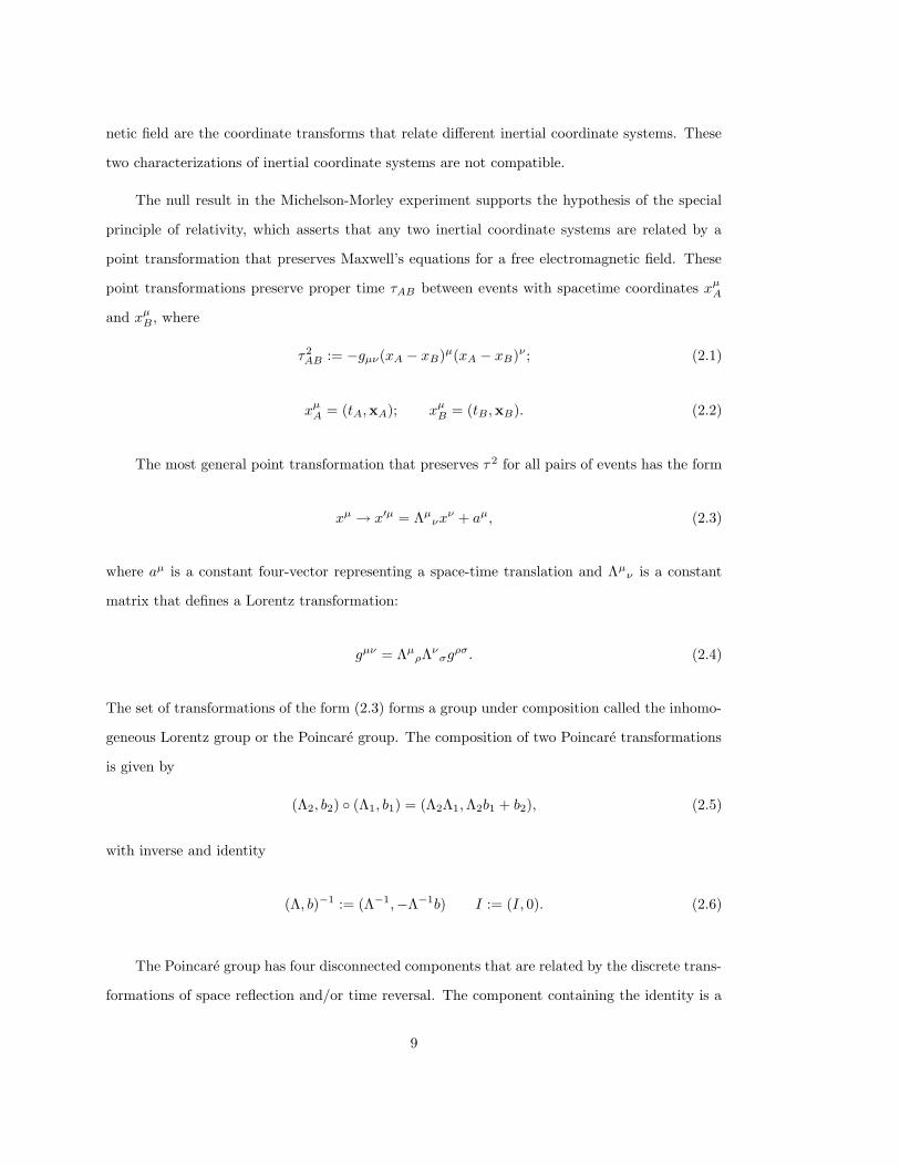
The null result in the Michelson-Morley experiment supports the hypothesis of the special

principle of relativity, which asserts that any two inertial coordinate systems are related by a

point transformation that preserves Maxwell’s equations for a free electromagnetic field. These

point transformations preserve proper time τAB between events with spacetime coordinates xµA

and xµB , where

τ2AB := −gµν(xA − xB)µ(xA − xB)ν ; (2.1)

xµA = (tA,xA); xµ

B = (tB ,xB). (2.2)

The most general point transformation that preserves τ 2 for all pairs of events has the form

xµ → x′µ = Λµνx

ν + aµ, (2.3)

where aµ is a constant four-vector representing a space-time translation and Λµν is a constant

matrix that defines a Lorentz transformation:

gµν = ΛµρΛ

νσg

ρσ. (2.4)

The set of transformations of the form (2.3) forms a group under composition called the inhomo-

geneous Lorentz group or the Poincare group. The composition of two Poincare transformations

is given by

(Λ2, b2) (Λ1, b1) = (Λ2Λ1,Λ2b1 + b2), (2.5)

with inverse and identity

(Λ, b)−1 := (Λ−1,−Λ−1b) I := (I, 0). (2.6)

The Poincare group has four disconnected components that are related by the discrete trans-

formations of space reflection and/or time reversal. The component containing the identity is a

9

subgroup which is distinguished by the conditions det|Λ| = 1 and Λ00 ≥ 1. These are called proper

(det|Λ| = 1) orthochronous (Λ00 ≥ 1) Lorentz transformations. The remaining components are

obtained by applying a time reversal, space reflection, or both, to a proper, orthochronous Lorentz

transformation. Although Maxwell’s equations are invariant under the full Poincare group, the

weak interaction is not invariant under those Poincare transformations involving the discrete

symmetries of time reversal and/or space reflection. It is customary to consider these discrete

symmetries separately from the continuous symmetries. In what follows, relativistic invariance

will refer to invariance under Poincare transformations associated with proper orthochronous

Lorentz transformations, or, equivalently, the Poincare transformations continuously connected

to the identity. In all that follows, references to the Poincare group will mean this subgroup, and

it will be assumed that any two inertial coordinate systems are related by a transformation in

this subgroup.

The principle of relativity is a statement that there is nothing in the laws of physics that

distinguishes different inertial coordinated systems:

A system satisfies the principle of special relativity if the results of equivalent experiments

done in different inertial coordinate systems are identical. A theory is consistent with the

principle of special relativity if the measurable predictions of the theory for equivalent exper-

iments done in different inertial coordinate systems are identical.

In classical physics, the solutions of the dynamical equations are observable. A classical

theory is relativistically invariant if the solution of a Poincare transformed equation is identical

the Poincare transformed solution of the original equation. This will follow if the equation

transforms covariantly under the action of the Poincare group.

In quantum physics, some modifications are required, because the measurable quantities are

not the solutions of the Schrodinger equation, but are instead probabilities constructed from scalar

products of two solutions of the Schrodinger equation. In general, the solutions of the Schrodinger

equation can be transformed by a large class of unitary transformations that change the form

of the equations and solutions but leave the probabilities unchanged. Clearly, invariance under

change of representation does not change the physics. Thus, in formulating the principle of special

relativity in quantum mechanics, it is appropriate to demand that the physically measurable

10

quantities, i.e., the probabilities associated with an isolated system, cannot be used to distinguish

different inertial coordinate systems. This is the point of view taken by (Wi 39) and refined by

Bargmann (Ba 54).

Before discussing Wigner’s formulation of relativistic invariance in quantum theories, it is

useful to give a brief historical review of relativistic quantum mechanics.

2.2. Historical Perspective

Almost as soon as Heisenberg and Schrodinger formulated nonrelativistic quantum mechan-

ics, considerable effort was aimed at finding a suitable relativistic quantum theory. The rela-

tivistic Schrodinger equation (Su 63, Du 83, Fr 83) is obtained from the correspondence principle

by replacing the nonrelativistic relation between energy and momentum with the corresponding

relativistic relation. The result for a free particle is:

i∂

∂tψ =

√−∇2 +m2 ψ. (2.7)

Although this equation is acceptable in principle, it was discarded because the square root in the

kinetic energy operator was difficult to utilize with interactions, and because of the non-symmetric

treatment of space and time.

These objections can be overcome by squaring Eq. (2.7), which gives the Klein-Gordon

equation (Sc 26, Kl 26, Go 26a, Go 26b, Fo 26a, Fo 26b, Ku 26, Do 26):

(∂

∂xµ

∂

∂xµ−m2)ψ = 0. (2.8)

The Klein-Gordon equation for a particle in a Coulomb field originally appeared in Schrodinger’s

1926 paper (Sc 26), but was discarded because it does not generate the experimentally observed

fine structure splitting in the Hydrogen spectrum. The Klein-Gordon equation has well known

problems. Because it is a second order equation in the time variable, probabilities constructed

out of the wave functions are not conserved in time. In addition, the energy spectrum is not

bounded from below. More recent investigations show that the predictions of the Klein-Gordon

equation are in good agreement with the experimental spectrum of mesonic atoms (De 79, Wo 80,

Fr 83).

11

The Dirac equation (Di 28):

(iγµ∂µ +m)ψ = 0, (2.9)

was designed to give a symmetric treatment of the space and time derivatives (for covariance)

and have probabilities that are conserved in time. Solutions to the Dirac equation for an electron

in the Coulomb field of a proton are in good agreement with the experimentally measured fine

structure splitting of the spectrum of the Hydrogen atom. The Dirac equation has an energy

spectrum that is not bounded from below, but this was fixed with Dirac’s “hole theory” (Di 30),

which predicted the existence of positrons. In spite of the difficulties with the energy spectrum,

following the discovery of positrons by Anderson in 1932 (An 32), the Dirac equation was believed

to be the correct equation for treating relativistic quantum mechanics until Pauli and Weisskopf

(Pa 34) reinterpreted the Klein-Gordon equation as an equation for a quantized field.

The quantization of the Electromagnetic field was motivated by physical consideration. Dirac

1927 (Di 27) gave the first quantum mechanical treatment of a particle interacting with a quan-

tized electromagnetic field. Heisenberg and Pauli (He 29) were the first to attempt to quantize

the full electromagnetic field.

The theory of quantized fields developed in the following years. The theory of quantized fields

allowed one to eliminate the concept of instantaneous action at a distance. The mathematical

difficulties with the theory made its acceptance slow. The acceptance of quantum electrodynamics

is in part due to the agreement of the calculated magnetic moment of the electron (Sc 48) and the

Lamb shift (Be 47) with the experimentally measured values (Fo 48, La 47). These calculations,

and confidence in the theory, have steadily improved over the subsequent years. The experimental

success of perturbative quantum electrodynamics has shown that quantum field theory with weak

coupling can provide a quantitative description of dynamics at currently accessible energies.

Although systematic expansions for physical observables can be found in perturbative quantum

electrodynamics, it is still not known how to give the complete mathematical interpretation of

the theory.

Today, especially with the discovery of asymptotically free (Po 73, Gr 73a, Gr 73b, Gr 74)

non-Abelian gauge theories (Ya 56), most physicists believe that the laws of physics at currently

12

accessible energies are governed by local relativistic field theories. At the same time, there are

no known non-trivial examples of field theories in 3+1 dimensions satisfying all of the physical

properties (axioms) expected of a local relativistic quantum field. What this means in practice

is that there are no known algorithms with ab initio error bounds that allow one to find a

solution of the field equations to arbitrary accuracy. Even in quantum electrodynamics, our

confidence comes from the comparison of theory with experiments, and not from a thorough

understanding of the theory. Physical arguments suggest that the radius of convergence (in the

coupling constant α) of the perturbation series in quantum electrodynamics is zero (Dy 52). For

quantum electrodynamics, these deficiencies are largely academic; however, for models of the

strong interactions, perturbative quantum field theory is manifestly inadequate.

Because the theoretical foundations of field theory have never been under complete control,

there has always been activity involved with the formulation of alternative methods for construct-

ing models of physical systems that combine relativity and quantum mechanics. Although one

can take the point of view that these alternative models should be considered at a fundamental

level, one must then explain any differences between the predictions of such models with those

of quantum electrodynamics. Alternatively, one does not have to consider these models as fun-

damental; they can be considered as phenomenologies that properly combine the principles of

quantum mechanics and relativity. It only needs to be demonstrated that such a phenomenology

provides a good quantitative description of the physics for a sufficiently large class of systems

under a sufficiently large class of conditions. For instance, one goal would be to find a model

of nucleon-nucleus scattering for all target nuclei for all energy transfers below 1 GeV. Nonrela-

tivistic quantum mechanics with phenomenological nucleon-nucleon interactions provides such a

model that is valid for energy transfers below the threshold for pion production. Relativity must

be included for higher energy transfers.

It is difficult to give a complete review of all of the alternative methods that have been

proposed to construct relativistic quantum mechanical models. This is in part because there are

so many different starting points and approaches which make it difficult to compare different

models. One thing that can be said at the outset is that in the same way that there are many

quantum theories with the same classical limit, there are also many relativistic models with the

same nonrelativistic limit. This means that the concept of a relativistic correction is meaningful

13

only within the context of a given model. Instead of giving a historic account of the various

attempts to construct quantum mechanical models, we give a brief discussion of some of the

fundamental issues involved in the development of such models, and a discussion of some of the

attempts used to deal with these issues. This will hopefully make it easier for the reader to make

a critical analysis of various approaches.

1. Quantum mechanics: This requires a linear theory, to ensure the superposition principle,

formulated on a Hilbert space. States of the system are represented by one dimensional sub-

spaces, or “rays,” of the Hilbert space. The square magnitude of the inner product between

two normalized state vectors represents the probability that if the system is prepared in the

state represented by one of the vectors that it will be measured to be in the state represented

by the second vector. There are two relevant comments. One is that the underlying Hilbert

space can be quite abstract, which turns out to be the case in local field theories (St 64)

and covariant quantum mechanical models (Po 85a). The second is that the more general

algebraic formulation of quantum mechanics (Vo 36) is relevant for treating systems with an

infinite number of degree of freedom (Ha 64).

One instance where questions about quantum mechanics become tricky occurs when ap-

proximate sets of equations for objects such as transition operators and Green functions

are obtained by truncation. In applications, equations such as Bethe-Salpeter equations

(Sa 51), Blankenbecler-Sugar (Bl 66) equations and the Gross equation (Gr 82a, Gr 82b),

are normally formulated with a kernel which, although motivated by field theory, is phe-

nomenological. Such phenomenological equations are called quasipotential equations, and

they are used for realistic calculations of the energy levels in positronium (Lo 63a, Lo 63b,

To 73). The solution of these equations is usually an observable of interest, and for such

applications, no further analysis is required. If one wants to compare these models to other

approaches, however, it is natural to want to be able to reconstruct the underlying quan-

tum model, i.e., the model Hilbert space and a unitary time translation operator, and to

extract either sufficient or necessary conditions on the structure of the input to allow such

a reconstruction. For the case of Green functions, the problem is to use time ordered Green

functions to construct the non-ordered Green functions (Wightman functions), which can

then be used to construct the quantum mechanics using the reconstruction theorem (St 64),

14

or the retarded Green functions, which can be used to reconstruct the field (Gl 57).

2. Relativistic Invariance: Relativity requires the existence of inertial coordinate systems

and physical equivalence of coordinate systems related by Lorentz transformations and space-

time translations. Wigner (Wi 39) analyzed this requirement for the case of quantum me-

chanics and found that it is equivalent to the existence of a unitary ray representation of the

Poincare group (inhomogeneous Lorentz group) on the quantum mechanical Hilbert space.

Note that the Schrodinger equation and the existence of the Hamiltonian are consequences

of applying Wigner’s analysis to invariance under time translations. The beauty of Wigner’s

theorem is that it is an inescapable consequence of the invariance of probabilities under

changes of inertial coordinate system.

Wigner’s theorem applies both to quantum theories of fields and of particles. It can be

satisfied in a variety of ways. One way is to construct an explicit representation of a uni-

tary representation of the Poincare group on the quantum Hilbert space. A second way is

to construct a representation of the infinitesimal generators of the Poincare group, which

are self-adjoint operators that satisfy commutation relations characteristic of the group. In

canonical field theories, these expressions are normally generated by integrating the energy-

momentum and angular momentum tensors over a suitable three dimensional surface (Sc 62,

Ch 73). A third way is to require that Poincare transformations are implemented by man-

ifest covariance, and find a representation of the Hilbert space for which these Poincare

transformations are unitary. This approach is used in axiomatic field theory (St 64), covari-

ant constraint dynamics (Lo 87, Po 85, Ri 85, Sa 86a, Sa 86b, Sa 88), and any non-trivial

manifestly covariant quantum theory.

Beyond these minimal requirements, there are many other important issues which are listed

below:

1. The spectral condition: This requires that the Hamiltonian of the theory has an energy

spectrum bounded from below. The invariance of quantum mechanical probabilities in time

implies the existence of a Hamiltonian. The spectral condition is essential for the theory to

be stable against spontaneous decay. The spectral condition is relevant because it is clearly

violated by the Klein-Gordon equation and the Dirac equation; although it is resolved in the

15

Dirac case by “hole theory.”

2. Einstein causality: This is also referred to as microscopic locality. It assumes the existence

of observables associated with arbitrarily small regions of spacetime, and the ability to make

independent measurements of any two such observables in causally disconnected regions. It

is this condition that requires an infinite number of degrees of freedom (i.e., independent

observables for every spacetime volume). This condition is independent both of relativistic

invariance and of the existence of a well defined initial value problem. When combined

with conditions imposed by relativity, quantum mechanics and the spectral condition, one

obtains the core of the “axioms of local quantum field theory.” Although there are many

sets of axioms (St 64, Ha 64, Os 75a, Os75 b, Ne 73, Fr 74), these are the main physical

assumptions that appear either directly or as consequences of any set of axioms. What is

relevant is that except for the case of the free fields, there are no known non-trivial models

in 3+1 dimensions that satisfy any of these sets of axioms. In this sense, Einstein causality

requires a local field theory.

Einstein causality is an idealization of a sensible macroscopic condition to arbitrarily small

volumes of spacetime. It is interesting to question whether this condition can be tested by

experiment. In order to make measurements in arbitrarily small laboratories, one needs to

transfer larger and larger momenta to the system. This requires a knowledge of asymptotic

properties of the theory at arbitrarily high energy and momenta. Tests of locality thus

involve probing models at all energy scales, which in turn requires an infinite number of

experiments. On the other hand, for each finite scale, one can argue that only a finite number

of quantum mechanical degrees of freedom is relevant. Haag and Swieca (Ha 65) showed that

for local fields with a particle interpretation, there is a finite number of quantum mechanical

degrees of freedom associated with any finite volume of classical phase space. This can be

interpreted to mean that experiments that probe any finite volume of classical phase space

cannot distinguish a model with a finite number of degrees of freedom from a local field

theory. These consideration suggest that Einstein causality cannot be tested by experiment,

although the axioms of field theory imply (St 64) that if it is satisfied up to a certain minimal

distance in all coordinated systems, then it must be valid for all distances.

16

It should be emphasized that there are many observed consequences of microscopic locality,

such as crossing symmetry, PCT , existence of antiparticles, etc. Although these properties

suggest an underlying local theory, all of them can be satisfied in nonlocal models of a finite

number of degrees of freedom.

3. Macroscopic locality: This is sometimes called cluster separability. It is the experimen-

tally relevant part of Einstein causality. It assumes that observables associated with regions

of spacetime that have a sufficiently large (as opposed to arbitrarily small) spacelike separa-

tion commute. This condition can be realized independently of Einstein causality (Os 74a).

The relevance of this condition was emphasized by Foldy (Fo 61, Fo 74). If the scattering

operator is considered to be the fundamental observable of the model, it requires cluster

properties of the scattering matrix (Co 65). This is essential in order to provide the con-

nection between few- and many-body physics. For systems of more than two particles, it is

known that in certain formulations of relativistic quantum mechanics, macroscopic locality

and the existence of a non-trivial scattering theory are manifestly incompatible (Mu 78).

4. Relativistic Scattering theory: This means that the S matrix should be relativistically

invariant. Fong and Sucher (Fo 64) exhibited a counterexample which shows that relativistic

invariance of the model does not imply relativistic invariance of the scattering matrix. They

also gave sufficient conditions for a model to have a Poincare invariant scattering matrix.

The problem is that the scattering asymptotic conditions must also be formulated in an

invariant way.

5. Connection to Classical Physics: There are a number of issues here that have led

to many difficulties. The simplest expectation is that the classical limit of a relativistic

quantum mechanical model should be relativistic classical mechanics. The difficulties start

with defining relativistic classical mechanics:

5.1 Canonical formulation: Dirac (Di 49) outlined a canonical approach to relativistic

classical mechanics, in which the Lie algebra of the Poincare group is realized in terms

of Poisson brackets. Poincare transformations are then implemented, at least locally, in

terms of canonical transformations.

5.2 World line condition: One classical notion, known as the world line condition, is

17

that the spacetime coordinates of classical particles should transform as four-vectors. It

turns out that this is incompatible with the existence of interactions in Dirac’s canonical

formulation of classical mechanics. This is the conclusion of the “no-go” theorem of Cur-

rie, Jordan and Sudarshan (Cu 63a, Cu 63b). The content of this theorem is that there

are three sets of Poisson bracket relations: those required by relativity (Di 49), those

involving the generalized coordinates and momenta, and those that define the world line

condition (Cu 63a, Cu 63b). These relations can only be satisfied simultaneously if the

model has no interactions. Because of this, there does not appear to be a classical limit

of the quantum theory with all of the desired properties. This problem has led to an in-

dustry that has tried various ways to get around this problem in the classical case, and to

construct quantum mechanical models with these limits. Classical many-time equations

(Va 65) provide one approach, but these equations are not canonical, and consequently

are difficult to quantize. Another approach, called covariant constraint dynamics, uses

Dirac’s generalized classical mechanics for constrained Hamiltonian system (Di 50), and

is reviewed in (Lo 87). The quantum mechanical version can be realized in a Hilbert

space setting by using the constraints to define a scalar product on the Hilbert space

(Po 85a, Ri 85, Sa 86a, Sa 86b, Sa 88). In this case, the scalar product is described

by a non-trivial kernel that plays the same role in quantum constraint dynamics as the

Wightman functions (Wi 65a) of quantum field theory. The kernels should be consistent

with the all of the axioms of the field theory except the locality axiom (Po 85a). The

main difficulties occur in simultaneously demanding both macroscopic locality and the

spectral condition.

5.3 Covariance: Covariance of classical wave equations is a consequence of relativistic in-

variance if the solutions are classical observables. For Maxwell’s equations, the electric

and magnetic fields must transform as a rank-two antisymmetric tensor density. The

vector potential, which is not observable, may be subject to non-covariant gauge con-

ditions. The same comment applies to quantum theories: if the solutions of a quantum

mechanical equation are observable, then they should transform covariantly, and if they

are not, then covariance is not required. This has been the source of some confusion.

In Dirac’s 1927 paper (Di 27), covariance was an essential element of the derivation,

18

although the solutions were interpreted as wave functions, which are not observable. It

is clear that one can construct unitary operators that transform the solutions and the

equation in a manner that destroys the covariance without changing the physics. In

spite of this observation, the focus historically of much work on relativistic quantum

mechanics has been one of maintaining covariance.

There are two different type of objects that transform covariantly in field theories.

The first class of objects involve matrix elements of covariant field operators between

physical states. This class includes current matrix elements, Bethe-Salpeter wave func-

tions (Sa 51) , Blankenbecler-Cook wave functions (Bl 60), and N -quantum amplitudes

(Gr 65a). These objects, which are sometime called wave functions, do not have the

usual quantum mechanical interpretation of a wave function, in the sense that there is no

scalar product for which these objects can be interpreted as vectors in a Hilbert space.

Nevertheless, matrix elements of operators between the corresponding physical states

can be expressed in terms of bilinear forms involving these matrix elements (Ma 55,

Hu 75).

The second class of covariant objects involves covariant wave functions that are true

wave functions, in the sense that there exists an inner product as discussed above.

These objects are computed in covariant constraint dynamics (Lo 87, Ri 85, Sa 86a,

Sa 86b, Sa 88). In this case, the covariance requires an interaction dependent scalar

product (Po 85a).

5.4 Retardation: This is the classical statement of Einstein causality. In a quantum the-

ory, it does not imply microscopic locality, and is not needed for macroscopic locality.

The first of these statements appeals to the axioms of field theory, where it is possible

to construct models with retardation that are Poincare invariant and satisfy the spec-

tral condition, but which violate some consequence of the full theory, such as crossing

symmetry. In this case, one of the axioms must be violated, and microscopic locality

is usually the troublesome axiom. Likewise, there exist models with instantaneous di-

rect interactions (i.e., that violate retardation) which are consistent with macroscopic

locality. The coordinates that are retarded in interactions are free-particle coordinates;

19

this is simply a choice of representation in a quantum mechanical theory. All that is

relevant about this representation is that these free particles have an asymptotic inter-

pretation, so that they can be used to formulate asymptotic conditions in a scattering

theory. The physics is not affected by unitary transformations that become the identity

asymptotically, but destroy the retardation in the interaction region.

The one unifying principle in all relativistic formulations is Wigner’s (1939) theorem. In a

quantum mechanical setting it gives a precise mathematical formulation of the invariance of quan-

tum probabilities under change of inertial coordinate systems. Wigner defined a quantum theory

to be Poincare invariant if and only if all quantum mechanical probabilities have values that are

independent of the choice of inertial coordinate system. A precise mathematical characterization

of this condition is given by the following theorem (Wi 39):

Theorem: (Wigner) A quantum mechanical model formulated on a Hilbert space preserves

probabilities in all inertial coordinate systems if and only if the correspondence between states

in different inertial coordinate systems can be realized by a unitary ray representation U(Λ, a)

of the Poincare group.

This result applies both to quantum field theories and to particle theories. Quantum field theories

have additional properties. Most notable of these is microscopic locality, which implies a model

with an infinite number of degrees of freedom, since it requires the existence of independent

observables associated with each arbitrarily small region of spacetime.

To understand the mathematical implementation of Wigner’s theorem, let H be the model

Hilbert space, and let X and X ′ be two inertial coordinate systems related by a Poincare trans-

formation (Λ, a). Consider an experiment viewed by an observer in X where a system is initially

prepared in a state |ψ〉 and detectors are prepared to measure the probability that the system is

in a state |φ〉. For states normalized to unity, the probability that this system is measured to be

in the state |φ〉 is:

P = |〈ψ|φ〉|2. (2.10)

Consider an equivalent experiment done by an observer in X ′. In this case, the system is initially

prepared in the state |ψ′〉 and detectors are prepared to measure the probability that the system

20

is in the state |φ′〉:

P ′ = |〈ψ′|φ′〉|2. (2.11)

Relativistic invariance demands that P = P ′, that is, the probability of obtaining this result

should be independent of where the laboratory is located, when the experiment is performed,

which direction the apparatus in oriented, and how fast the laboratory is moving relative to

another inertial coordinate system. Wigner’s theorem implies that if the above applies to all

pairs of (normalizable) vectors and all inertial coordinate systems, then the vectors |ψ〉 and |ψ ′〉

(resp. |φ〉 and |φ′〉 ) are related by a correspondence of the form

|ψ′〉 = eiθU(Λ, a)|ψ〉, (2.12)

where U(Λ, a) is unitary and satisfies the group representation property:

U(Λ2, a2)U(Λ1, a1) = eiφ(2,1)U(Λ2Λ1, a2 + Λ2 · a1). (2.13)

The phases appear because physical states are only defined up to phase. Bargmann gave a

refinement of Wigner’s theorem that removes the phase in (2.13). This is discussed in Section 3.

The specification of U(Λ, a) on H defines a relativistic quantum mechanical model. Note

that U(Λ, a) contains the time evolution subgroup, and thus includes the dynamics. In relativistic

quantum mechanics, the construction of U(Λ, a) replaces the construction of the unitary time

evolution operator in nonrelativistic quantum mechanics.

The construction of relativistic quantum mechanical models of interacting particles was not

vigorously pursued after Wigner stated his theorem. On the other hand, as phenomenologies,

they fill in a gap that exists between the nonrelativistic quantum mechanics and local relativistic

field theories. The construction of U(Λ, a) is necessarily more complicated than the construction

of the time evolution operator in nonrelativistic quantum mechanics, as will be discussed below.

One non-trivial consequence of special relativity is that it involves the Poincare group rather

than the Lorentz group. The complicating feature is that the Poincare group includes the time

evolution subgroup. Because time is also involved in Lorentz transformations, this requires that

21

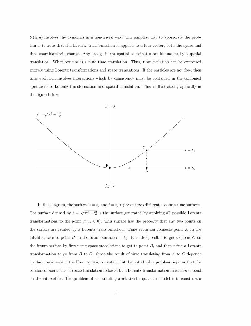
U(Λ, a) involves the dynamics in a non-trivial way. The simplest way to appreciate the prob-

lem is to note that if a Lorentz transformation is applied to a four-vector, both the space and

time coordinate will change. Any change in the spatial coordinates can be undone by a spatial

translation. What remains is a pure time translation. Thus, time evolution can be expressed

entirely using Lorentz transformations and space translations. If the particles are not free, then

time evolution involves interactions which by consistency must be contained in the combined

operations of Lorentz transformation and spatial translation. This is illustrated graphically in

the figure below:

A

B

C

••

•

x = 0

t = t1

t = t0

t =√

x2 + t20

fig. 1

......................

.......

.............

..........

.........................................

..................................................................................................................................................................................................................................................................................................................................................................................................................................................................................................................................................................................................................................................................

..................................

..............................................................................................................................................................................................................................................................................................................................................................................................................................................................................

.......

...

.......

...

.......

...

.......

...

.......

...

.......

...

.

In this diagram, the surfaces t = t0 and t = t1 represent two different constant time surfaces.

The surface defined by t =√

x2 + t20 is the surface generated by applying all possible Lorentz

transformations to the point (t0, 0, 0, 0). This surface has the property that any two points on

the surface are related by a Lorentz transformation. Time evolution connects point A on the

initial surface to point C on the future surface t = t1. It is also possible to get to point C on

the future surface by first using space translations to get to point B, and then using a Lorentz

transformation to go from B to C. Since the result of time translating from A to C depends

on the interactions in the Hamiltonian, consistency of the initial value problem requires that the

combined operations of space translation followed by a Lorentz transformation must also depend

on the interaction. The problem of constructing a relativistic quantum model is to construct a

22

unitary representation of the Poincare group consistent with time evolution in the sense discussed

above.

Note also from Fig. 1 that there are many different possible formulations of the initial value

problem in relativistic theories. In the diagram, both the fixed time surface and the Lorentz

invariant surface have the property that all points on each surface have a relative space-like sep-

aration and each surface intersects every possible world line once and only once. Clearly, either

one, but not both, of these surfaces would make a suitable initial value surface. In general there

is an infinite number of possible initial value surfaces. The interaction dependence of the repre-

sentation of the Poincare group ensures the compatibility of these choices. These complications

do not arise nonrelativistically because in that case, with the speed that defines the “light cone”

unbounded, the constant time surface is the only surface on which all points have a relative

space-like separation.

To summarize, experimentally it is found that there are coordinate systems where free par-

ticles move with constant linear momentum and that any two such systems are related by a

Poincare transformation. The laws of physics are blind to the choice of inertial coordinate sys-

tems. In quantum theories, it is found that this is true if and only if there exists a unitary ray

representation of the Poincare group on the quantum mechanical Hilbert space.

Direct construction of models based on these ideas was initiated by Dirac’s work on the

Hamiltonian formulation of the classical dynamics of particles (Di 49). Classical Hamiltonian

systems have the advantage that they can be used to construct quantum systems by canonical

quantization. In the Hamiltonian formulation of classical mechanics, the goal is to construct a

representation of the Poincare group as a group of canonical transformations on phase space.

Dirac analyzed these requirements infinitesimally, and showed that the problem is equivalent to

the construction of a representation of the Lie algebra of the Poincare group in terms of Poisson

brackets that includes interactions in a consistent way. Although Dirac did not solve the problem,

he did show that it could be reduced to one of three simpler non-linear problems. These simpler

realizations are based upon the observation that the Poincare group has several subgroups (Pa

75, Le 78) that do not involve the Hamiltonian explicitly. The Lie algebra can be constructed

consistently by assuming that the generators of one of these subgroups contains no interactions.

23

The general problem is non-linear, since interactions must be added to all 10 generators in a

manner that preserves the Lie algebra.

These three methods of realizing the Lie algebra are called Dirac’s forms of the dynamics.

They go by the name “instant,” “front” and “point” forms. The names are characteristic of

the subgroups that are chosen to contain no interactions. In the “instant” form, it is the set of

Poincare transformations which leave the instant plane, t = tc, invariant. In the “point” form, it

is the subgroup that leaves the Lorentz invariant surface t2 − x2 = c2 invariant. In the “front”

from, it is the subgroup which leaves the light front, x+ = x0 + x3 = 0, invariant. A more

complete discussion can be found in Dirac’s original review and a paper by Leutwyler and Stern

(Le 78).

The first construction of a relativistic quantum mechanical model of two interacting particles

based on these ideas was given by Bakamjian and Thomas (Ba 53). The non-linear problem

defined by Dirac is solved in the quantum mechanical case by realizing the Lie algebra of the

Poincare group in terms of commutators of Hermitian operators rather than Poisson brackets

of functions on classical phase space. Bakamjian and Thomas used Dirac’s “instant form” of

the dynamics. Foldy (Fo 61) pointed out the importance of cluster separability or macroscopic

locality in these models.

The work of Bakamjian and Thomas was extended to the case of three particles by Coester

(Co 65). Sokolov (So 75, So 77, So 78a, So 78b) extended this work to the “point form” and

“front form” of the dynamics, the N -body problem with cluster properties, and models involving

particle production. Leutwyler and Stern (Le 78) formulated the two-body problem in the “front

form.” Coester and Polyzou (Co 82) formulated models in all three forms, with cluster properties

for arbitrary numbers of particles, and a limited class of models with particle production. Polyzou

(Po 89) has extended the Bakamjian-Thomas construction for two particles to a general group-

theoretic setting for which Dirac’s forms of the dynamics appear a special cases of a general

construction. Lev (Le 83) has reviewed the three-body problem in the front form . Three-body

calculations have been discussed in the instant form by Glockle et al. (Gl 86), and in the front

form by Kondratyuk and Terent’ev (Ko 80), by Bakker, et al. (Ba 79), and by Cao and Keister

(Ca 90). Meson form factors in quark/parton models have been studied by Terent’ev (Te 76),

24

by Chung, et al. (Ch 86, Ch 88b), and by Dziembowski (Dz 88b). Meson-nucleon scattering

with pion absorption has been examined by Berestetskii (Be 81). Various aspects of electron-

deuteron elastic scattering and breakup have been studied in the instant form by Coester and

Ostebee (Co 75), and in the front form by Kondratyuk and collaborators (Ko 83, Ko 84, Gr 84), by

Chung and collaborators (Ch 88a, Ch 89) and by Keister (Ke 88). Related front-form work based

upon field theory can be found in the review of Frankfurt and Strikman (Fr 81). Nucleon form

factors have been examined in the front form by Berestetskii and Terent’ev (Be 76, Be 77), by

Dziembowski (Dz 88a, Dz 88b), and by Chung and Coester (Ch 90). Nuclear structure functions

have been reviewed by Berger and Coester (Be 85, Be 87).

Two examples of the Bakamjian-Thomas construction are given in the next two sections.

One is a model of confined quarks in the “instant” form, and the other is a model of nucleon-

nucleon scattering in the “front” form. In each case, the model is constructed first for spinless

constituents, and then extended to spin- 12 constituents. For both examples, the models are

analytically solvable.

25

2.3. Example: Confined Spinless Quarks

We now consider a simple model of two spinless quarks of mass m with a confining inter-

action. The first step is to determine the mass spectrum. In quantum mechanics, this is done

by computing the eigenvalues of a self-adjoint operator that represents the mass, or rest energy,

of the bound system. The mass M plays the same role in relativistic models as the internal

Hamiltonian h in nonrelativistic models.

The basis states of the Hilbert space for this model can be taken as the tensor products of

single-particle states:

|p1 p2〉 := |p1〉 ⊗ |p2〉. (2.14)

Equivalently, we can change variables and use state vectors labeled by the total momentum P

and relative momentum k of two free quarks. The total momentum is defined as

P := p1 + p2. (2.15)

To construct the relative momentum vector k, let L−1c (Q) be the rotationless Lorentz trans-

formation that transforms the momentum of two non-interacting quarks to zero. The relative

momentum is defined as the three-vector components of

kµ := L−1c (Q0)

µνp

ν1 . (2.16)

The rotationless Lorentz transformation L−1c (Q) is defined by its action on a four-vector Aµ:

(A′0

A′

)= L−1

c (Q)

(A0

A

)=

(A0√

1 + Q2 − Q · A

A −A0Q + Q (Q · A)(1 +√

1 + Q2)−1

). (2.17)

The quantity Q0 = P/M0 is the four-velocity of the non-interacting system, where

M0 := (H20 − P2)

12 ; H0 := ωm(p1) + ωm(p2), (2.18)

and

ωm(p) :=√m2 + p2. (2.19)

26

The three-vector part of k is then given by the variable change

k = k(p1,p2) = p1 +P

M0

[P · p1

M0 +H0− ωm(p1)

]. (2.20)

If the plane-wave states are given delta function normalizations, i.e.,

〈p′1 p′2|p1 p2〉 = δ(p′1 − p1)δ(p′2 − p2); 〈P′ k′|Pk′〉 = δ(P′ − P)δ(k′ − k), (2.21)

then the state vectors |Pk〉 and |p1 p2〉 are related to each other via

|Pk〉 :=

∣∣∣∣∂(p1 p2)

∂(Pk)

∣∣∣∣12

|p1 p2〉 (2.22)

where the Jacobian in Eq. (2.22) is

∣∣∣∣∂(p1 p2)

∂(Pk)

∣∣∣∣ =ωm(p1)ωm(p2)M0

ωm(k)ωm(k)ωM0(P)

. (2.23)

The angles k can be eliminated in favor of discrete quantum numbers using spherical harmonics:

|kl;Pµ〉 :=

∫dkY l

µ(k)|k;P〉. (2.24)

The Hilbert space then consists of the set of functions 〈kl;Pµ|Ψ〉, with scalar product

〈Ψ|Φ〉 :=∞∑

l=0

l∑

µ=−l

∫d3P

∞∫

0

k2dk 〈kl;Pµ|Ψ〉∗〈kl;Pµ|Φ〉, (2.25)

where 〈Pk|Ψ〉 satisfying

〈Ψ|Ψ〉 <∞. (2.26)

The mass operator M is assumed to be the sum of an operator M0 that represents the

27

invariant mass of two non-interacting quarks, plus a phenomenological confining interaction:

M = M0 + U. (2.27)

For computational purposes, it is convenient to write equation (2.27) in the form

M2 = M20 + V, (2.28)

where U and V are related by

V = M0, U+

+ U2. (2.29)

Equations (2.27) and (2.28) are equivalent: the choice between them is a matter of convenience.

To be consistent with experimental observation, the interaction must chosen so that M has only

positive eigenvalues.

In the basis (2.24), the non-interacting Hamiltonian and mass operator are multiplication

operators:

H0(P,k ) :=√M2

0 + P2; M0 = M0(k ) := 2√m2 + k2. (2.30)

The eigenvalue problem for the square of the mass is:

〈kl;Pµ|4(m2 + k2) + V |P ′Ψ〉 = λ2〈kl;Pµ|P′Ψ〉. (2.31)

In applications, the interaction V , or equivalently U , is determined by the physics of the system

being modeled. An analytically solvable choice is to take V so that in the representation (2.25),

Eq. (2.31) is equivalent to the eigenvalue problem for a harmonic oscillator. The following V has

this property:

〈k′l′;P′µ′|V |kl;Pµ〉 := − 1

g4δl′lδµ′µδ(P

′ − P)1

k2δ(k′ − k)∇2

kl, (2.32)

where g is a constant with dimensions of length, and ∇2kl is the partial wave Laplacian:

∇2kl = − 1

k2

d

dkk2 d

dk+l(l + 1)

k2. (2.33)

The corresponding U is obtained from Eq. (2.29).

28

With this interaction, the eigenvalue problem for the mass operator is analytically solvable.

Equation (2.31) can be put in the form

(−∇2kl + 4g4k2)〈kl;µ|Ψ〉 = g4(λ2 − 4m2)〈kl;µ|Ψ〉, (2.34)

where

〈kl;P′µ′|PΨ〉 = δ(P′ − P)〈kl;µ|Ψ〉, (2.35)

which is mathematically equivalent to the eigenvalue problem for a three dimensional harmonic

oscillator.

The following mass spectrum results from diagonalizing M 2 and taking the square roots of

the eigenvalues:

Mnl := λnl = 2√m2 + (2n+ l + 3

2 )/g2. (2.36)

Note that Mnl is positive for all n and l. It represents the mass of a physical particle (meson)

with intrinsic angular momentum l. The spectrum for the mass operator is the square root of a

shifted oscillator spectrum, rather than the oscillator spectrum itself. It is interesting to compare

this spectrum to that obtained from a mass operator of the form

M ′ = 2√m2 + k2 +

c1r

+ c2r, (2.37)

which is motivated by quark phenomenology (Ca 83a). The parameters in (Ca 83a) arem = 0.313

GeV, c1 = 0.5 and c2 = 0.197 GeV2. The spectrum for this operator is to be compared to

Eq. (2.36) with the same quark mass, with the parameter g adjusted so the nominal rms ground

state oscillator radius is 0.54 fm, namely, the weighted (3:1) average of the ρ and π meson

Compton wavelengths. This corresponds to g = 1.59 GeV−1. For the case n = 0 and l = 0, 1, 2, 3

the meson spectra predicted by these two different mass operators (Ca 83a, Po 87) are given in

Table 1:

29

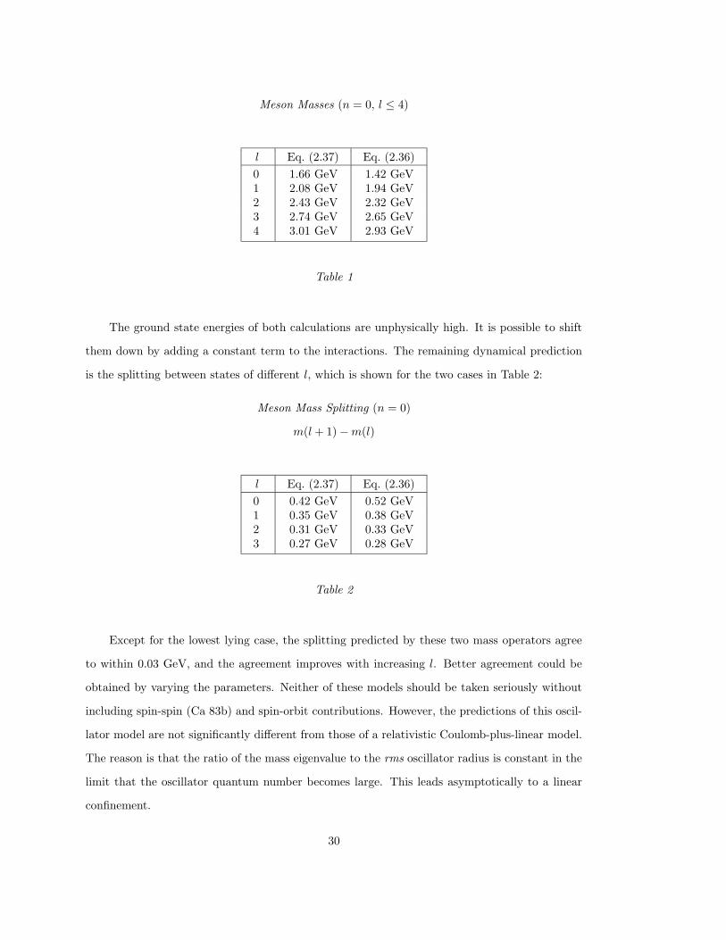
Meson Masses (n = 0, l ≤ 4)

l Eq. (2.37) Eq. (2.36)

0 1.66 GeV 1.42 GeV1 2.08 GeV 1.94 GeV2 2.43 GeV 2.32 GeV3 2.74 GeV 2.65 GeV4 3.01 GeV 2.93 GeV

Table 1

The ground state energies of both calculations are unphysically high. It is possible to shift

them down by adding a constant term to the interactions. The remaining dynamical prediction

is the splitting between states of different l, which is shown for the two cases in Table 2:

Meson Mass Splitting (n = 0)

m(l + 1) −m(l)

l Eq. (2.37) Eq. (2.36)

0 0.42 GeV 0.52 GeV1 0.35 GeV 0.38 GeV2 0.31 GeV 0.33 GeV3 0.27 GeV 0.28 GeV

Table 2

Except for the lowest lying case, the splitting predicted by these two mass operators agree

to within 0.03 GeV, and the agreement improves with increasing l. Better agreement could be

obtained by varying the parameters. Neither of these models should be taken seriously without

including spin-spin (Ca 83b) and spin-orbit contributions. However, the predictions of this oscil-

lator model are not significantly different from those of a relativistic Coulomb-plus-linear model.

The reason is that the ratio of the mass eigenvalue to the rms oscillator radius is constant in the

limit that the oscillator quantum number becomes large. This leads asymptotically to a linear

confinement.

30

The eigenvectors of the oscillator model can be labeled by a principal quantum number, an

orbital quantum number, the total linear momentum of two free quarks, and a magnetic quantum

number:

|nl;Pµ〉. (2.38)

With the internal wave functions 〈k|nlµ〉 normalized to unity, the normalization of the vectors

(2.38) is determined by Eq. (2.35) to be:

〈n′l′;P′µ′|nl;Pµ〉 = δn′nδl′lδµ′µδ(P′ − P). (2.39)

The wave functions of these state vectors in the plane wave basis are related to standard nonrel-

ativistic harmonic oscillator wave functions φnl(k)Ylµ(k) by

〈kl′;P′µ′|n l;Pµ〉 = δl′lδµ′µδ(P′ − P)φnl(k). (2.40)

The wave functions 〈kl;P′µ|nl;Pµ〉 and the spectrum (2.36) represent the dynamical solution

of this model. Note that the dynamics of this model are determined by the mass operator, or,

equivalently, the square of the mass operator. The total momentum does not appear in the

dynamical equations (2.34) or (2.37). The solutions |nl;Pµ〉 are simultaneous eigenstates of the

mass and linear momentum. However, the model is not yet relativistic.

To interpret the model relativistically, we must construct a unitary representation U(Λ, a) of

the Poincare group, which defines the transformation properties of these states under changes of

inertial coordinate systems. The representation must be consistent with the dynamics developed

above. This is done by defining certain basic Poincare transformations between pairs of eigen-

states of the four-momentum, and then fixing the remaining transformations by group theory.

This procedure is straightforward, but not unique. The construction in this section will be done

in a manner that leads to an instant form of dynamics, namely, one in which the Euclidean sub-

group, consisting of space translations and rotations, acts in a manner that is independent of the

mass eigenvalue. In an instant-form dynamics, the Euclidean subgroup is called the “kinematic

subgroup.”

31

It is important to note that solving the eigenvalue problem for the mass operator is separate

from the specific choices that lead to an instant-form dynamics. In particular, given the eigen-

states |nl;Pµ〉, one can construct different forms of the dynamics by making different choices

concerning which eigenstates states are related by a given Poincare transformation. There are

many ways in which this can be done that are both consistent with the group theory and the

dynamics. The examples with scattering which follow the confining models exhibit a different

choice, which leads to a front-form dynamics.

The construction is based on the following observation: for a particle of mass Mln and

spin l, the transformation properties of states of that particle are fixed uniquely by the set of

transformations that leave the particle at rest, along with the action of one specific momentum

dependent transformation that associates states of the particle at rest to states where it has

momentum P. A general Poincare transformation can be written as a Lorentz transformation,

followed by a spacetime translation:

U(Λ, a) = T (a)U(Λ), (2.41)

where the following shorthand notation has been introduced:

T (a) := U(I, a); U(Λ) := U(Λ, 0). (2.42)

We define the transformation for spacetime translations of a mass eigenstate with mass eigenvalue

Mnl and zero total momentum in a manner consistent with this dynamics:

T (a)|nl; 0µ〉 := e−iMnla0 |nl; 0µ〉. (2.43)

The action of a pure rotation on a rest eigenstate with intrinsic angular momentum l is defined

so that the rest state transforms as a spin-l irreducible representation under rotations:

U(R)|nl; 0µ〉 :=∑

µ

|nl; 0µ〉Dlµµ(R). (2.44)

We now define the action of the rotationless Lorentz transformation Lc(Q) which maps the rest

32

eigenstate to the corresponding eigenstate with momentum P:

U [Lc(Qnl)] |nl; 0µ〉 :=

√ωMnl

(P)

Mnl|nl;Pµ〉. (2.45)

The coefficient with the square root is needed to ensure unitarity of U [Lc(Qnl)] if the states

are normalized according to Eq. (2.39). Different choices of normalization will lead to different

coefficients. The transformation depends on the four-velocity Qµ = Qµnl = Pµ

nl/Mnl of the

interacting system.

Equations (2.43), (2.44) and (2.45) can be combined with the group representation property

to define U(Λ, a) uniquely on all states. This in turn defines a relativistic quantum mechanics.

Note that Eqs. (2.43), (2.44), (2.45) and the group representation properties define a represen-

tation of U(Λ, a). This is not the only possible representation consistent with this dynamics, as

will be shown in later examples.

To show how Eqs. (2.43)-(2.45) define U(Λ, a) on all states, consider an arbitrary Lorentz

transformation Λ, and define the transformed four-momentum and four-velocity by

P ′µnl := ΛµνP

νnl; Q′µnl := Λµ

νQνnl. (2.46)

To determine the effect of an arbitrary Lorentz transformation Λ on a state vector, consider the

successive transformations

R(Λ, Qnl) := L−1c (Q′nl) ΛLc(Qnl) (2.47)

that map the three momentum as follows: 0 → P → P′ → 0. Since the transformation R(Λ, Qnl)

maps the rest four-velocity (1, 0, 0, 0) onto itself, it is therefore a rotation, often called a Wigner

rotation. Equation (2.47) implies that we can write

Λ = Lc(Q′nl)R(Λ, Qnl)L

−1c (Qnl), (2.48)

and therefore, assuming the group representation property, the unitary transformation U(Λ) can

33

be expressed as:

U(Λ) = U [Lc(Q′nl)]U [R(Λ, Qnl)]U

[L−1

c (Qnl)]. (2.49)

This is used to compute the action of U(Λ, a) on an arbitrary eigenvector |nl;Pµ〉. Applying the

transformations in Eq. (2.49) from right to left, we utilize Eq. (2.45), followed by Eq. (2.44), and

finally Eq. (2.45) again to get

U(Λ)|nl;Pµ〉 =

√ωMnl

(P′)ωMnl

(P)

∑

µ

|nl;P′µ〉Dlµµ [R(Λ, Qnl)] . (2.50)

The action of T (a) can be computed by observing that T (a)U(Λ) = U(Λ)T (Λ−1a), which, to-

gether with Eqs. (2.43) and (2.50), yields

U(Λ, a)|nl;Pµ〉 = eiP ′

nl·a

√ωMnl

(P′)ωMnl

(P)

∑

µ

|nl;P′µ〉Dlµµ [R(Λ, Qnl)] . (2.51)

Equation (2.51) expresses the action of U(Λ, a) on an eigenstate as a linear combination of eigen-

states of the same physical mass Mnl and spin l, with uniquely determined algebraic coefficients.

This defines the action of U(Λ, a) on a basis of eigenstates of M , and thus completes a specific

construction of U(Λ, a).

The operator U(Λ, a) defines a relativistic quantum mechanics which is consistent with

Wigner’s theorem. It specifies the desired correspondence between states in two different in-

ertial coordinate systems in a manner that preserves all probabilities, and is consistent with the

dynamics defined by Eq. (2.34).

The interaction dependence of an arbitrary Lorentz transformation that is demanded from

the diagram in Fig. 1 appears in the Wigner rotation, the normalization factor [ωMnl(P′)/ωMnl

(P)]12 ,

and the phase factor eiP ′

nl·a through the dependence on the mass eigenvalue Mnl. In this rep-

resentation, for the special case of a pure spatial translation, there is no Wigner rotation, the

normalization factor is unity, and the phase factor is eiP·a. This means that the coefficients of the

transformation do not depend on the mass eigenvalue. For the case of a pure rotation, there is no

34

phase factor, the normalization factor is unity, and the Wigner rotation Rc(R,Qnl) corresponding

to a rotation Λ = R can be calculated using Eqs. (2.17) and (2.47), with the result:

Rc(R,Qnl) = R, (2.52)

which is independent of the mass eigenvalue. It follows that in the representation (2.51), the

subgroup generated by spatial translations and rotations has the same effect on all mass eigen-

states, independent of their mass eigenvalue. This property is a consequence of our definition of

U(Λ, a). A relativistic model with this property is called an instant-form dynamics. The property

(2.52) is characteristic of Wigner rotations associated with rotationless Lorentz transformations

only. In other forms of dynamics, such as the front form, Eq. (2.17) is replaced with a different

transformation, and the corresponding Wigner rotation of the rotation R generally depends on

the mass eigenvalue.

Equation (2.51) can be used to compute matrix elements of U(Λ, a) in the basis of eigenstates

of the mass operator:

〈n′l′;P′µ′|U(Λ, a)|nl;Pµ〉 = δn′nδl′lδ(P′ − PΛnl)e

iP ′

nl·a

×√ωMnl

(P′)ωMnl

(P)Dl

µ′µ [R(Λ, Qnl)] ,(2.53)

where PΛnl = ΛPnl is the transformed four-momentum. In the basis of plane-wave states |Pk〉,

the transformation U(Λ, a) can be obtained by inserting a complete set of mass eigenstates and

using Eqs. (2.53) and standard properties of the rotation group:

〈P′ k′|U(Λ, a)|Pk〉 =∑

nl

δ(P′ − PΛnl)δ(k′ −R(Λ, Qnl)k])

× eiP ′

nl·aφnl(k′)φ∗nl(k),

(2.54)

where φnl(k) is a radial momentum wave function, and

Pnl = Pnl(p1 + p2) :=(ωMnl

(p1 + p2),p1 + p2

). (2.55)

35

In the tensor-product basis |p1 p2〉, Eq. (2.54) becomes

〈p′1 p′2|U(Λ, a)|p1 p2〉 =∑

nl

δ(p′1 + p′2 − ΛPnl)δ(k′ −R(Λ,Qnl)k)eiP ′

nl·a

×√ωMnl

(PΛ)

ωMnl(P)

∣∣∣∣∂(p′1p

′2)

∂(P′k′)

∣∣∣∣

12∣∣∣∣∂(p1p2)

∂(Pk)

∣∣∣∣

12φnl(k

′)φ∗nl(k).

(2.56)

The interaction dependence enters Eqs. (2.54) and (2.56) in the l- and n-dependent quantities

in the Jacobian factors, in the phase factor, and in the Wigner rotations that rotate the relative

momentum vector. These expressions illustrate the complexity of U(Λ, a) when it is expressed in

a plane wave basis. These expressions are used when a relativistic two-body system is imbedded

in a many-body system.

It is useful to examine the nonrelativistic limit of this model, and compare it to the familiar

nonrelativistic harmonic oscillator. A nonrelativistic limit can be obtained formally by assuming

that

m >> k2, V. (2.57)

The mass operator is then expressed as a power series in

ζ :=hNR

m:=

k2

m2+

V

4m2, (2.58)

where hNR is the nonrelativistic Hamiltonian. However, since both k2 and V are unbounded

operators and m is a c-number, it is not clear that the limit (2.57) or the expansion (2.58) is

ever meaningful. This is a general problem which accompanies expansions about a nonrelativistic

limit in relativistic quantum mechanical models. Nevertheless, the above assumption is the one

usually made, and we will trace its implications for this particular model.

The expansion can be written as follows:

M =√

4(m2 + k2) + V

= 2m

[1 +

∞∑

n=1

(−)n−1(2n− 3)!!

2nn!ζn

]

= 2m+ hNR + 2m

[ ∞∑

n=2

(−)n−1(2n− 3)!!

2nn!ζn

].

(2.59)

In the nonrelativistic limit, only the first two terms are kept.

36

The exact eigenvalue equation can be expressed as follows:

M2|ψ〉 = [4(m2 + k2) + V ]|ψ〉 = (4m2 + 4mhNR)|ψ〉 = λ2|ψ〉. (2.60)

That is, |ψ〉 is also an eigenstate of hNR:

hNR|ψ〉 = (λ2 − 4m2

4m)|ψ〉, (2.61)

where λ is the exact eigenvalue of M . In the nonrelativistic limit, the eigenvalue equation is

hNR|ψ〉 = (λNR − 2m)|ψ〉. (2.62)

The eigenstates |ψ〉 in Eqs. (2.61) and (2.62) are the same, with eigenvalue

η = η(n, l) =2n+ l + 3

2

4mg2, (2.63)

but the correspondence between η(n, l) and the mass spectra λ and λNR is not. The difference is

|λ− λNR| = 2m√

1 + η/m− 1 − η/2m. (2.64)

For small η/m, the right-hand side of Eq. (2.64) is of order (η/m)2. The relativistic correction

to the spectrum is small for sufficiently low lying states, i.e., for values of n and l such that

(2n+ l + 32 ) 4m2g2.

For models in which an interaction V is added to the square of the free mass operator,

the eigenvalues change in the nonrelativistic limit, but the state vectors do not. However, the

interpretation of the state vectors in terms of wave functions is also different in the nonrelativistic

37

limit. In our model, two-body wave functions have the form

〈p1p2|nl;Pµ〉 =

∣∣∣∣∂(Pk)

∂(p1 p2)

∣∣∣∣12

δ(p1 + p2 − P)φnlµ(k), (2.65)

where

k = p1 +P

M0

[P · p1

M0 +H0− ωm(p1)

]. (2.66)

In the nonrelativistic limit, we have

NR〈p1p2|nl;Pµ〉 = δ(p1 + p2 − P)φnlµ(kNR), (2.67)

where

kNR = 12 (p1 − p2). (2.68)

These expressions of wave functions in terms of one-body degrees of freedom typically appear

in calculations where the two-body system is embedded in a larger system, or an external probe is

introduced. Thus, even though the nonrelativistic limit has the same state vector as the original

model, calculations which employ the wave functions in Eqs. (2.65) and (2.67) will yield different

results. Whether these differences can be interpreted in terms of a systematic expansion in powers

of hNR/m is not at all certain, since hNR is an unbounded operator.

38

2.4. Example: Confined Relativistic Quarks - With Spin

We now consider an extension of the previous model in which spin- 12 quarks are bound by a

confining interaction.

In the example of spinless quarks just given, it was useful to work in a plane-wave basis

|kl;Pµ〉, characterized by the total momentum P, the relative momentum k and the orbital

angular momentum l of the non-interacting system. This suggests that we use basis states

|[ls]kj;Pµ〉 for models with spin. The state vectors labelled in this way can also be written

in terms of tensor products of single-particle basis states in a manner similar to that of the

previous section. We could proceed as before by showing the explicit connection between the

tensor-product states and this partial-wave basis. Since this connection represents a change of

basis only, and does not affect the discussion of dynamics which follows, it will be deferred to

the end of this section. However, tensor products of single-particle states are frequently used in

calculations which go beyond the two-body problem, either in terms of an external probe or a

few-body system, and the connection to the partial-wave basis is not always the same as one finds

in a nonrelativistic approach. The reader is therefore encouraged to examine that discussion, even

though it does not bear directly on the development of a dynamical model which follows.

The labels l and s do not correspond to physical observables. Nevertheless, we anticipate in

advance that for two spin- 12 particles, s can take on the values 0 or 1, and the relative orbital

angular momentum can take on any non-negative integer value. The model Hilbert space is taken

to be the space of functions 〈[ls]kj;Pµ|Ψ〉, satisfying

〈Ψ|Ψ〉 <∞, (2.69)

where the scalar product is given by

〈Ψ|Φ〉 :=

∫

R3

d3P

∞∫

0

k2dk

∞∑

j=0

j∑

µ=−j

1∑

s=0

|j+s|∑

l=|j−s|〈[l s]k j;Pµ|Ψ〉∗〈[l s]k j;Pµ|Φ〉. (2.70)

In this representation, the square of the non-interacting mass operator is still the multipli-

39

cation operator:

M20 := 4(m2 + k2). (2.71)

The form of the eigenvalue problem for the square of the mass is unchanged from the spinless

case:

〈[ls]kj;Pµ|[4(k2 +m2) + V

]|Ψ〉 = λ2〈[ls]kj;Pµ|Ψ〉, (2.72)

except that the interaction can now have additional degrees of freedom. For the spin- 12 case, an

interaction V that leads to a solvable dynamical model is:

〈[l′s′]k′j′;P′µ′|V |[ls]kj;Pµ〉 := − 1

g4js

δj′jδµ′µδs′sδl′lδ(P′ − P)

1

k2δ(k′ − k)∇2

kl, (2.73)

where gjs is a constant with dimensions of length. The interaction now depends on the spin s,

the orbital angular momentum l, and the intrinsic angular momentum j. Since this interaction

commutes with the total three-momentum, the intrinsic angular momentum, and the operators

whose eigenvalues are l and s, the eigenstates of the mass operator can be taken to be simultaneous

eigenstates of the operators whose eigenvalues are j,P, µ, l, and s:

〈[l′s′]k′j′;P′µ′|[ls]nj;Pµ〉 = δj′jδµ′µδs′sδl′lδ(P′ − P)φl′s′n′j′(k), (2.74)

where φlsnj(k) is the solution of

(−∇2kl + 4g4

jsk2)φlsnj(k) = g4

js(λ2n − 4m2)φlsnj(k), (2.75)

which is identical to the eigenvalue equation (2.34) in the spinless case. The oscillator functions

φlsnj(k) are normalized to unity, which implies the following normalization for the eigenstates:

〈[l′s′]n′j′;P′µ′|[ls]nj;Pµ〉 = δj′jδµ′µδs′sδl′lδn′nδ(P′ − P). (2.76)

The following mass spectrum results from diagonalizing M 2 and taking the square roots of

the eigenvalues:

Mlsnj = λlsnj = 2√m2 + (2n+ l + 3

2 )/g2js. (2.77)

This is similar to the mass spectrum in the spinless case, except for the dependence upon l and

s in addition to j and n. Note that Mlsnj is positive for all n, j, l and s, as required.

40

The eigenstates |[ls]nj;Pµ〉 form a basis on the Hilbert space. In the representation (2.74),

the only difference between this case and the spinless case is the appearance of the degeneracy

parameters l and s, which appear in both the mass eigenstates and plane-wave basis elements.

In general, a two-body interaction need not be diagonal in l and s. When that is the case,

the quantum numbers l and s no longer appear as labels of the eigenstates, although they are

variables in the wave functions.

To develop a representation of the Poincare group for our harmonic-oscillator model using

instant-form dynamics, one simply takes over the entire development surrounding Eqs. (2.43)–

(2.51), with the substitution Mnl → Mlsnj . The actions of translations, rotations, and rotation-

less boosts on states with P = 0 are defined as follows:

T (a)|[ls]nj;0µ〉 := e−iMlsnj ·a|[ls]nj;0, µ〉 (2.78)

U(R)|[ls]nj;0µ〉 :=∑

µ

|[ls]nj;0, µ〉Djµµ(R) (2.79)

U [Lc(Qlsnj)]|[ls]nj;0µ〉 :=

√ωMlsnj

(P)

Mlsnj|[ls]nj;P, µ〉. (2.80)

The group representation property can then be used again to give the general transformation law

for the eigenstates of the four momentum and intrinsic angular momentum:

U(Λ, a)|[ls]nj;Pµ〉 = eiΛP ·a√ωMlsnj

(PΛ)

ωMlsnj(P)

|[ls]nj;PΛ, µ〉Djµµ[R(Λ, P )], (2.81)

where

PΛ := ΛPlsnj , (2.82)

corresponding to Eq. (2.51) in the spinless case. In this basis, matrix elements of U(Λ, a) have

the form

〈[l′s′]n′j′;P′µ′|U(Λ, a)|[ls]nj;Pµ〉 = δs′sδµ′µδn′nδl′lδ(P′ − PΛ)eiPΛ·a

×√ωMnljs

(P′)

ωMnljs(P)

D(l)µ′µ [Rc(Λ, Qnljs)] .

(2.83)

Equation (2.81) defines a unitary representation of the Poincare group consistent with the

dynamics defined by Eq. (2.72), and thus represents a non-trivial relativistic quantum mechanical

41

model. Note that there are two steps to this general process. First, one finds a simultaneous set

of eigenstates of the mass and spin. In the oscillator example, the oscillator coupling constant

is adjusted to obtain the best fit to the measured mass/spin spectrum. After this is done, one

defines a unitary representation of the Poincare group that relates different eigenstates. Relativity

does not affect the fitting of the mass/spin spectrum of the mesons, but the mass/spin spectrum

constrains the transformation properties. Relativity becomes important in processes where two

different inertial coordinate systems become relevant. Examples include the interaction of a

two-body system with an external probe such as an electron, or a two-body subsystem within a

many-body problem.

We end the discussion of this example by providing the connection between the basis states

|[ls]kj;Pµ〉 and the tensor-product states:

|p1µ1 p2µ2〉 := |p1µ1〉 ⊗ |p2µ2〉. (2.84)

To construct the relative momentum basis, we need to introduce a “free-particle dynamics”. The

single-quark states are assumed to transform under a one-body representation of the Poincare

group like a bound state of mass Mnl and spin l in Eq. (2.51), with Mnl replaced by the quark

mass m, and l replaced by 12 . We denote this transformation by U1(Λ, a) for quark 1 and U2(Λ, a)

for quark 2. The tensor product of the single-particle transformations is

U0(Λ, a) := U1(Λ, a) ⊗ U2(Λ, a) (2.85)

This is purely a kinematic definition that facilitates the construction of a variable change; it has

nothing to do with the physical interacting representation of the Poincare group.

We begin by defining a new vector labelled by relative and total momenta:

|k;Pµ1µ2〉 :=

∣∣∣∣∂(p1 p2)

∂(Pk)

∣∣∣∣12

|p1µ1 p2µ2〉, (2.86)

where the relevant kinematic relations and Jacobians are given above. We now consider the set of

state vectors |k;0µ1µ2〉, corresponding to a non-interacting two-body system at rest. The angles

42

k can be eliminated in favor of discrete quantum numbers using spherical harmonics:

|kl;0µlµ1µ2〉 :=

∫dkY l

µl(k)|k;0µ1µ2〉. (2.87)

We now wish to couple the spins and the internal angular momentum together. Under rotations,

a single-particle state |piµi〉 transforms as follows:

Ui(R)|piµi〉 =∑

µi

|Rpiµi〉D12µiµi

(R). (2.88)

We have chosen the single-particle states to have the same properties as outlined in the previous

example, namely, that the states |0iµi〉 and |piµi〉 are related by kinematic rotationless boosts,

which means that the Wigner rotation in Eq. (2.88) is in fact the rotation R. Combining the

properties of the spherical harmonic, we find that the state vector |k;0µ1µ2〉 transforms as follows

under the rotation U0(R):

U0(R)|kl;0µlµ1µ2〉 =∑

|kl;0µlµ1µ2〉Dlµlµl

(R)D12µ1µ1

(R)D12µ2µ2

(R). (2.89)

Since the rotation matrices all contain the same argument, the indices can be combined using

standard rotational Clebsch-Gordan coefficients to define a new state vector:

|[ls]kj;0, µ〉 :=∑

〈 12µ1

12µ2|sµs〉〈lµlsµs|jµ〉|kl;0µlµ1µ2〉. (2.90)

Under rotations, this state transforms as follows:

U0(R)|[ls]kj;0, µ〉 =∑

|[ls]kj;0µ〉Djµµ(R). (2.91)

The state vector |[ls]kj;Pµ〉 describes two free particles with total three-momentum P. The

total four-momentum of the free-particle system is therefore

P0 := ((ωm(p1) + ωm(p2),P). (2.92)

We now apply a noninteracting rotationless boost to the state |[ls]kj;0, µ〉:

|[ls]kj;Pµ〉 :=

√M0

ωM0(P)

U0[Lc(P0/M0)]|[ls]kj;0µ〉, (2.93)

where M20 = P 2

0 is the square of the mass of the free-particle system. Note that the action of

43

U0[Lc(pi/mi)] induces Wigner rotations on the product states:

U0[Lc(P0/M0)]|kµ1 − kµ2〉 =

√ωm(p1)

ωm(k)

√ωm(p2)

ωm(k)

∑|p1µ1 p2µ2〉

×D12µ1µ1

[R(Lc(P/M0), k1/m)]D12µ2µ2

[R(Lc(P/M0), k2/m)],(2.94)

where

ki := L−1c (P0/M0)pi. (2.95)

For half-integer spins, the arguments of the Wigner rotations in Eq. (2.94) should be specified

using SU(2) in order to get the correct phase. This is discussed further in the following sections.

Putting everything together, we get

|[ls]kj;Pµ〉 =

∣∣∣∣ωm(p1)ωm(p2)M0

ωm(k)ωm(k)ωM0(P)

∣∣∣∣12 ∑∫

dkY lµl

(k)

× 〈 12µ1

12µ2|sµs〉〈lµlsµs|jµ〉|p1µ1 p2µ2〉

×D12µ1µ1

[R(Lc(P/M0), k1/m)]D12µ2µ2

[R(Lc(P/M0), k2/m)].

(2.96)

Given the above definitions, these vectors are normalized as follows:

〈[l′s′]k′j′;P′µ′|[ls]kj;Pµ〉 = δµ′µδl′lδs′sδj′jδ(P′ − P)

1

k2δ(k′ − k). (2.97)

The action of U(Λ, a) in the tensor-product basis is obtained by combining Eqs. (2.96) and

(2.83):

〈p1µ1p2µ2|U(Λ, a)|[ls]nj;Pµ〉

= δ(p1 + p2 − PΛ)

√ωMnl

(PΛ)

ωMnl(P)

∣∣∣∣∂(p′1p

′2)

∂(P′k′)

∣∣∣∣

12∣∣∣∣∂(p1p2)

∂(Pk)

∣∣∣∣

12

× eiΛPlsnj ·aφlsnj(k)∑

Y lµ′

l(k)〈 1

2 µ112 µ2|sµs〉〈lµlsµs|jµ〉

×D12µ1µ1

[R(Lc(ΛQlsnj), k1/m)]D12µ2µ2

[R(Lc(ΛQlsnj), k2/m)]

×Djµµ[Rc(Λ, Plsnj)].

(2.98)

As in the spinless case, these equations again illustrate the complexity of U(Λ, a) when it is

expressed in a plane-wave basis. Their use may be required when a two-body system is imbedded

in a larger system.

44

2.5. Example: Spinless Two-Particle Scattering

In this section, a solvable relativistic model of two spinless particles of mass m that exhibits

scattering is constructed. This model is formulated using “front-form” dynamics. The light front

is the three-dimensional surface in spacetime characterized by the condition x+ = x0 + x3 =

0. This surface has the property that it is invariant under a seven-parameter subgroup of the

Poincare group. The subgroup includes a three-parameter subgroup of spacetime translations,

a three-parameter subgroup of “front-form” boosts, and a one-parameter subgroup of rotations.

These transformations are discussed in detail in Sections 3, 4, and Appendix B. In a front-form

dynamics, the unitary transformations U(Λ, a) contain no interactions for (Λ, a) restricted to this

seven-parameter subgroup, which replaces the Euclidean subgroup as the kinematic subgroup in

a front-form dynamics. A front-form dynamics has the following properties:

i. It has the largest (7 parameters) possible kinematic subgroup in a dynamical model. It is the

only kinematic subgroup containing both three independent boosts and three independent

spacetime translations.

ii. Because the “front-form” boosts form a subgroup (unlike the set of rotationless boosts),

there are no Wigner rotations associated with front-form boosts. There are, however, Wigner

rotations associated with other Lorentz transformations.

Apart from illustrating a solvable two-body scattering problem, the purpose of the construc-

tion in this section is to illustrate the similarities and differences in relation to the instant-form

constructions used to formulate the quark models above. As was mentioned earlier, the treatment

of the mass eigenvalue problem is separate from the choice of dynamics in constructing a unitary

representation of the Poincare group.

In practice the construction of a front-form dynamics is almost identical to that of an instant

form dynamics. It is a two-step process. The first step, which does not depend on the form of

dynamics, is to construct simultaneous eigenstates of the four-momentum and the spin. The

second is to define a unitary representation of the Poincare group that relates eigenstates with

the same mass and spin. The form of the dynamics is not fixed until the second step.

Before introducing the dynamics, we must select a set of plane-wave basis states. As with the

45

previous examples, we seek a partial-wave representation as the basis of choice for implementing

the dynamics. We show here the explicit steps needed to obtain this basis, starting from tensor

products of single-particle states:

|p1 p2〉 := |p1〉 ⊗ |p2〉, (2.99)

where p1 and p2 are the light-front components of the four-momenta p1 and p2, and p is defined

by:

p := (p⊥, p+); p⊥ := (p1, p2); p+ := p3 + p0. (2.100)

These three components of the four-momentum generate translations tangent to the three-surface

x+ = 0 (the light front). The components of p make up what we call a light-front vector. The

remaining component of the four momentum, p− := p0 − p3, is related to the mass operator by

the relation

p− :=m2 + p2

⊥p+

. (2.101)

The operator p− generates spacetime translations normal to the light front (i.e., along the x+

axis), and thus plays the role of the Hamiltonian in a front-form dynamics.

Transformations Lf (Q) which leave the light front invariant and transform the rest four-

velocity (1, 0, 0, 0) to the four-velocity Q are called front-form boosts. They have the property

that for any four-vector A:

A+′

A′⊥

A−′

= Lf (Q)

A+

A⊥

A−

=

Q+A+

A⊥ + Q⊥A+

(Q+)−1(Q2⊥A

+ + 2Q⊥ · A⊥ +A−)

. (2.102)

The composition of two front-form boosts yields a third front-form boost, which means that

the set of transformations Lf (Q) forms a subgroup. It also means that the three light-front

components of the four-momentum transform among themselves.

46

As in the instant-form example above, we now switch to state vectors labeled by the total

light-front momentum P and relative momentum k of two free quarks. The total momentum is

defined as

P := p1 + p2. (2.103)

The relative momentum k is equal to the three-momentum of particle 1 when P = 0, where

0 := (P⊥ = 0, P+ = M). (2.104)

For arbitrary p1 and p2, k is defined by applying a front-form boost to p1:

k := L−1f (Q0)p1, (2.105)

where Q0 = P/M0 is the four-velocity of the non-interacting system, and

M0 := (P+P−0 − P2⊥)

12 ; P−0 :=

m2 + p21⊥

p+1

+m2 + p2

2⊥p+2

. (2.106)

The three-vector part of k is then k = (k⊥, k3), where

k⊥ =p+2

P+p1⊥ − p+

1

P+p2⊥; k3 = 1

2 (p+1 − p+

2 )

√m2 + k2

⊥p+1 p

+2

. (2.107)

Note that the three-vector k as defined in Eq. (2.105) and given explicitly in Eq. (2.107) is

not the same three-vector k as defined in Eq. (2.16) and given explicitly in Eq. (2.20). While

they both give a relative three-momentum for a zero-momentum plane-wave state, the Lorentz

transformations used to obtain each k are not the same. Since the two forms of k must have

the same invariant length and are purely spatial, they must differ only by a rotation. If the

plane-wave states are given delta-function normalizations, i.e.,

〈p′1 p′2|p1 p2〉 = δ(p′1 − p1)δ(p′2 − p2); 〈P′ k′|P k〉 = δ(P′ − P)δ(k− k′), (2.108)

47

then the state vectors |P k〉 and |p1 p2〉 are related to each other via

|P k〉 :=

∣∣∣∣∂(p1 p2)

∂(P k)

∣∣∣∣12

|p1 p2〉, (2.109)

where the Jacobian in Eq. (2.109) is

∣∣∣∣∂(p1 p2)

∂(P k)

∣∣∣∣ =p+1 p

+2 M0

ωm(k)ωm(k)P+. (2.110)

The angles k can be eliminated in favor of discrete quantum numbers using spherical har-

monics:

|kl; Pµ〉 :=

∫dkY l

µ(k)|k; P〉. (2.111)

The Hilbert space for this model is taken to be the space of functions 〈kl; Pµ|Ψ〉, with scalar

product

〈Ψ|Φ〉 :=∞∑

l=0

l∑

µ=−l

∞∫

0

dP+

∫d2P⊥

∞∫

0

k2dk 〈kl; Pµ|Ψ〉∗〈kl; Pµ|Φ〉. (2.112)

In this basis, P denotes light-front components of the four-momentum

P = (P⊥, P+) P⊥ := (P 1, P 2) P+ := P 0 + P 3. (2.113)

The relative momentum k is related to the invariant mass of two non-interacting nucleons by

M20 = 4(m2 + k2), (2.114)

and l is the relative orbital angular momentum.

48

An interacting mass operator M can be constructed in the same manner as the previous

examples by adding an interaction to M0:

M = M0 + U. (2.115)

As in the case of the quark model, it is useful to define the interaction as the difference of the

squares of the interacting and non-interacting mass operators:

M2 = M20 + V. (2.116)

The interactions U and V are related by Eq. (2.29). As in the case of the quark model, the

interactions must be such that M 2 has positive eigenvalues. This requirement is more restrictive

in models that have scattering than in confining models because the mass of bound states is lower

than the rest mass of the constituent non-interacting particles. The spectral condition, M ≥ 0,

is violated when the binding energy exceeds the rest mass of the non-interacting system.

The interaction V is taken to be a rank-one separable interaction in each partial wave:

〈k′ l′; P′ µ′|V |k l; Pµ〉 := δl′lδµ′µδ(P′ − P)V l(k′, k), (2.117)

where

δ(P′ − P) := δ2(P′⊥ − P⊥)δ(P ′+ − P+), (2.118)

and

V l(k′, k) := −glfl(k′)fl(k)

∗. (2.119)

The form factors fl(k) and coupling constants gl represent the phenomenological input to this

model. The eigenvalue problem for M 2 is solvable up to a quadrature involving fl(k). The

structure of this operator differs from the interaction appearing in the quark model in that it

contains a delta function in the light-front vector components of the four-momentum, rather than

the three-vector components of the four-momentum.

49

Eigenstates of the four-momentum are eigenstates of both M 2 and P−, where

P− =M2 + P2

⊥P+

(2.120)

is the “front-form Hamiltonian” that generates translations normal to the light front. To solve

for the eigenvectors, it is convenient to use the eigenvalue equation for M 2:

M2|Ψ(−)〉 = λ2|Ψ(−)〉, (2.121)

which can be expressed in integral form as:

|Ψ(−)〉 = |Ψ0〉 +1

λ2 −M20 + i0+

V |Ψ(−)〉, (2.122)

where |Ψ0〉 must be a solution of

(M20 − λ2)|Ψ0〉 = 0. (2.123)

Note that the (−) superscript on the scattering state indicates an asymptotic condition as t →

−∞, corresponding to the +i0+ prescription in the denominator of the integral equation (2.122).

The mass eigenvalue for the scattering state is the invariant mass of the incident plane wave

state:

λ2 = 4(k2 +m2). (2.124)

For the interaction (2.117), the solutions 〈k′l′; P′µ′|kl; Pµ(−)〉 of Eq. (2.122) can be taken to

be simultaneous eigenstates of P and µ:

〈k′l′; P′µ′|kl; Pµ(−)〉 = δl′lδµ′µδ(P′ − P)φ

(−)kl (k′), (2.125)

where

φ(−)kl (k′) :=

1

k2δ(k′ − k) − glfl(k

′)f∗l (k)

(4k2 − 4k′2 + i0+)∆l(λ2), (2.126)

and

∆l(λ2) := 1 + gl

∞∫

0

k2dkf∗l (k)fl(k)

λ2 − 4m2 − 4k2 + i0+. (2.127)

The scattering eigenstates defined by Eq. (2.125) have the same normalization as the plane-

50

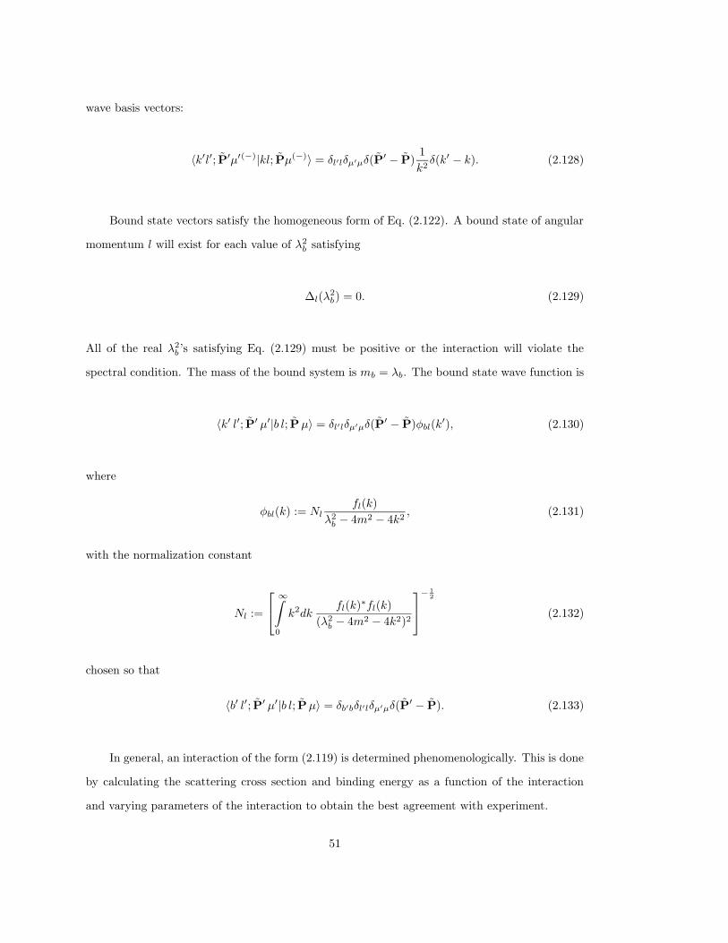
wave basis vectors:

〈k′l′; P′µ′(−)|kl; Pµ(−)〉 = δl′lδµ′µδ(P′ − P)

1

k2δ(k′ − k). (2.128)

Bound state vectors satisfy the homogeneous form of Eq. (2.122). A bound state of angular

momentum l will exist for each value of λ2b satisfying

∆l(λ2b) = 0. (2.129)

All of the real λ2b ’s satisfying Eq. (2.129) must be positive or the interaction will violate the

spectral condition. The mass of the bound system is mb = λb. The bound state wave function is

〈k′ l′; P′ µ′|b l; Pµ〉 = δl′lδµ′µδ(P′ − P)φbl(k

′), (2.130)

where

φbl(k) := Nlfl(k)

λ2b − 4m2 − 4k2

, (2.131)

with the normalization constant

Nl :=

∞∫

0

k2dkfl(k)

∗fl(k)

(λ2b − 4m2 − 4k2)2

− 1

2

(2.132)

chosen so that

〈b′ l′; P′ µ′|b l; Pµ〉 = δb′bδl′lδµ′µδ(P′ − P). (2.133)

In general, an interaction of the form (2.119) is determined phenomenologically. This is done

by calculating the scattering cross section and binding energy as a function of the interaction

and varying parameters of the interaction to obtain the best agreement with experiment.

51

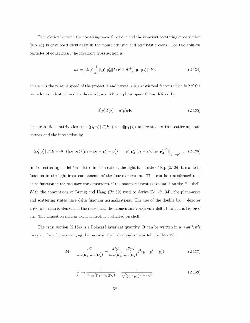
The relation between the scattering wave functions and the invariant scattering cross section

(Mo 45) is developed identically in the nonrelativistic and relativistic cases. For two spinless

particles of equal mass, the invariant cross section is

dσ = (2π)41

sv|〈p′1 p′2‖T (E + i0+)‖p1 p2〉|2dΦ, (2.134)

where v is the relative speed of the projectile and target, s is a statistical factor (which is 2 if the

particles are identical and 1 otherwise), and dΦ is a phase space factor defined by

d3p′1d3p′2 = d4p′dΦ. (2.135)

The transition matrix elements 〈p′1 p′2‖T (E + i0+)‖p1 p2〉 are related to the scattering state

vectors and the interaction by

〈p′1 p′2‖T (E + i0+)‖p1 p2〉δ(p1 + p2 − p′1 − p′2) = 〈p′1 p′2|(H −H0)|p1 p(−)2 〉

∣∣∣p−=p′−

. (2.136)

In the scattering model formulated in this section, the right-hand side of Eq. (2.136) has a delta

function in the light-front components of the four-momentum. This can be transformed to a

delta function in the ordinary three-momenta if the matrix element is evaluated on the P− shell.

With the conventions of Brenig and Haag (Br 59) used to derive Eq. (2.134), the plane-wave

and scattering states have delta function normalizations. The use of the double bar ‖ denotes

a reduced matrix element in the sense that the momentum-conserving delta function is factored

out. The transition matrix element itself is evaluated on shell.

The cross section (2.134) is a Poincare invariant quantity. It can be written in a manifestly

invariant form by rearranging the terms in the right-hand side as follows (Mo 45):

dΦ → dΦ

ωm(p′1)ωm(p′2)=

d3p′1ωm(p′1)

d3p′2ωm(p′2)

δ4(p− p′1 − p′2); (2.137)

1

v→ 1

vωm(p1)ωm(p2)=

1√(p1 · p2)2 −m4

; (2.138)

52

and the transition matrix element by the invariant matrix elements:

〈p′1 p′2‖T (E + i0+)‖p1 p2〉 → M;

M := 4(2π)6√ωm(p′1)ωm(p′2)〈p′1 p′2‖T (E + i0+)‖p1 p2〉

√ωm(p1)ωm(p2). (2.139)

The invariant amplitude M has the same normalization as the amplitude M in the Review of

Particle Properties (Yo 88).

As was the case in the instant-form quark models, it is convenient to use V rather than U in

order to make contact with phenomenology. We must therefore replace H−H0 by V = M2−M20

in Eq. (2.136), making use of the following:

(H −H0) =1

2(P− + P+ − P−0 − P+) =

1

2

(P2⊥ +M2

P+− P2

⊥ +M20

P+

)

=1

2P+(M2 −M2

0 ) =V

2P+.

(2.140)

The last quotient in Eq. (2.140) is well defined because P+ commutes with V in this model.

We must also replace the representations used to describe the initial and final states with

those used to formulate our dynamical equations:

|p1 p2〉 =

∣∣∣∣∣∂(P k)

∂(p1 p2)

∣∣∣∣∣

12

Y l∗µ (k)|k l; Pµ〉. (2.141)

Note that the single-particle states are labelled with ordinary three-momenta rather than light-

front momenta. However, k is defined according to Eq. (2.105). The Jacobian is

∣∣∣∣∣∂(P k)

∂(p1 p2)

∣∣∣∣∣ =ωm(ωm(k)ωm(k)P+

p1)ωm(p2)M. (2.142)

By means of the identification

〈k′l′; P′µ′|V |kl; Pµ(−)〉 = δl′lδµ′µδ(P′ − P)〈k′l′‖V ‖kl(−)〉, (2.143)

53

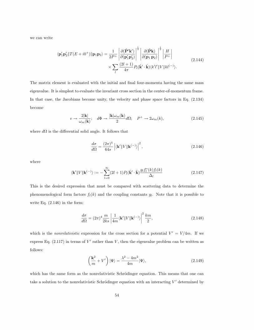
we can write

〈p′1p′2‖T (E + i0+)‖p1p2〉 =1

2P+

∣∣∣∣∣∂(P′k′)∂(p′1p

′2)

∣∣∣∣∣

12∣∣∣∣∣∂(Pk)

∂(p1 p2)

∣∣∣∣∣

12 ∣∣∣∣

H

P+

∣∣∣∣

×∑

l

(2l + 1)

4πPl(k

′ · k)〈k′l′‖V ‖kl(−)〉.(2.144)

The matrix element is evaluated with the initial and final four-momenta having the same mass

eigenvalue. It is simplest to evaluate the invariant cross section in the center-of-momentum frame.

In that case, the Jacobians become unity, the velocity and phase space factors in Eq. (2.134)

become

v → 2|k|ωm(k)

; dΦ → |k|ωm(k)

2dΩ; P+ → 2ωm(k), (2.145)

where dΩ is the differential solid angle. It follows that

dσ

dΩ=

(2π)4

64s

∣∣∣〈k′‖V ‖k(−)〉∣∣∣2

, (2.146)

where

〈k′‖V ‖k(−)〉 := −∞∑

l=0

(2l + 1)Pl(k′ · k)

glf∗l (k)fl(k)

∆l(2.147)

This is the desired expression that must be compared with scattering data to determine the

phenomenological form factors fl(k) and the coupling constants gl. Note that it is possible to

write Eq. (2.146) in the form:

dσ

dΩ= (2π)4

m

2ks

∣∣∣∣1

4m〈k′‖V ‖k(−)〉

∣∣∣∣2km

2, (2.148)

which is the nonrelativistic expression for the cross section for a potential V ′ = V/4m. If we

express Eq. (2.117) in terms of V ′ rather than V , then the eigenvalue problem can be written as

follows:(

k2

m+ V ′

)|Ψ〉 =

λ2 − 4m2

4m|Ψ〉, (2.149)

which has the same form as the nonrelativistic Schrodinger equation. This means that one can

take a solution to the nonrelativistic Schrodinger equation with an interacting V ′ determined by

54

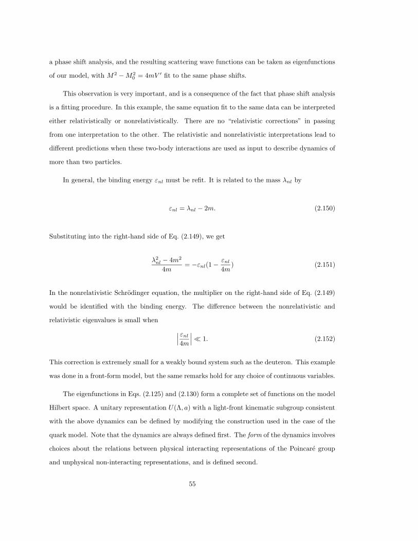
a phase shift analysis, and the resulting scattering wave functions can be taken as eigenfunctions

of our model, with M2 −M20 = 4mV ′ fit to the same phase shifts.

This observation is very important, and is a consequence of the fact that phase shift analysis

is a fitting procedure. In this example, the same equation fit to the same data can be interpreted

either relativistically or nonrelativistically. There are no “relativistic corrections” in passing

from one interpretation to the other. The relativistic and nonrelativistic interpretations lead to

different predictions when these two-body interactions are used as input to describe dynamics of

more than two particles.

In general, the binding energy εnl must be refit. It is related to the mass λnl by

εnl = λnl − 2m. (2.150)

Substituting into the right-hand side of Eq. (2.149), we get

λ2nl − 4m2

4m= −εnl(1 − εnl

4m) (2.151)

In the nonrelativistic Schrodinger equation, the multiplier on the right-hand side of Eq. (2.149)

would be identified with the binding energy. The difference between the nonrelativistic and

relativistic eigenvalues is small when

∣∣∣ εnl

4m

∣∣∣ 1. (2.152)

This correction is extremely small for a weakly bound system such as the deuteron. This example

was done in a front-form model, but the same remarks hold for any choice of continuous variables.

The eigenfunctions in Eqs. (2.125) and (2.130) form a complete set of functions on the model

Hilbert space. A unitary representation U(Λ, a) with a light-front kinematic subgroup consistent

with the above dynamics can be defined by modifying the construction used in the case of the

quark model. Note that the dynamics are always defined first. The form of the dynamics involves

choices about the relations between physical interacting representations of the Poincare group

and unphysical non-interacting representations, and is defined second.

55

In the instant-form quark model, the representation U(Λ, a) was defined so that the magnetic

quantum number of a zero-momentum eigenstate state |nl; (P = 0)µ〉 does not change when Λ

is a rotationless Lorentz transformation Lc(Q) . In a front-from dynamics, the representation

U(Λ, a) is defined so that the magnetic quantum number of a zero-momentum eigenstate |nl; 0µ〉

does not change when Λ is a kinematic front-form boost Lf (Q), where Q := P/M is the four-

velocity, and M is the mass eigenvalue of the interacting state. In this case, the rest eigenstate

corresponds to

P = 0 := (P⊥ = 0, P+ = M). (2.153)

We are now in a position to define a unitary representation of the Poincare group that (1) is

consistent with the dynamics (2.122) and (2) has the kinematic subgroup of the light front. As

in the instant-form examples discussed earlier, this is done by defining the action of spacetime

translations and rotations on the rest eigenstates of the four-momentum and the action of one

boost for each value of the four-velocity that relates states with any fixed momentum to states

with zero momentum. Thus, we define translations and rotations on the rest scattering eigenstates

by

T (a)|k l; 0µ(−)〉 := e−iMa0 |k l; 0µ(−)〉, (2.154)

and

U(R)|k l; 0µ(−)〉 :=l∑

µ=−l

|k l; 0 µ(−)〉Dlµµ(R), (2.155)

respectively. Front-form boosts on the rest eigenstates are defined by

U [Lf (P )]|k l; 0µ(−)〉 :=

√P+

M|k l; Pµ(−)〉, (2.156)

where the multiplicative factor in Eq. (2.156) is needed for unitarity with the normalization

(2.128). We must also define the action of U(Λ, a) on the rest eigenstates of the bound system:

T (a)|b l; 0µ〉 := e−iMba0 |b l; 0µ〉; (2.157)

56

U(R)|b l; 0µ〉 :=l∑

µ=−l

|b l; 0 µ〉Dlµµ(R); (2.158)

U [Lf (P )]|b l; 0µ〉 :=

√P+

Mb|b l; Pµ〉. (2.159)

These relations, together with the group representation property, fix the form of U(Λ, a) on all

states. This construction is similar to that in Eqs. (2.44)–(2.51): it makes use of the fact that

any Poincare transformation can be expressed as a composition of four basic transformations:

U(Λ, a) = U [Lf (ΛQ)]T [L−1f (ΛQ)a]U [Rf (Λ, Q)]U [L−1

f (Q)], (2.160)

The transformation Rf (Λ, Q) := L−1f (ΛQ)ΛLf (Q) is a front-form Wigner rotation: it maps

the rest four-velocity (1, 0, 0, 0) onto itself. However, since Rf (Λ, Q) employs front-form boosts

rather than rotationless boosts, it has different properties from those of Rc(Λ, Q) defined in the

instant-form examples in the previous sections. First, because the set of front-form boosts form a

closed subgroup, there is no Wigner rotation associated with a front-form boost. However, unlike

the case in the instant form, the Wigner rotation corresponding to an arbitrary rotation is not

necessarily the rotation itself. Only for pure rotations about the z axis (i.e., an element of the

kinematic subgroup) are the rotations the same.

Applying these transformations to a state with four-momentum P = MQ, and using Eqs. (2.154)–

(2.159), we obtain, with P ′ := ΛP :

U(Λ, a)|k l; Pµ(−)〉 = eiP ′·a√P ′+

P+

l∑

µ=−l

|k l; P′ µ(−)〉Dlµµ[Rf (Λ, Q)] (2.161)

for scattering states, and

U(Λ, a)|b l; Pµ〉 = eiP ′·a√P ′+

P+

l∑

µ=−l

|b l; P′ µ〉Dlµµ[Rf (Λ, Q)] (2.162)

for bound states. The transformation properties of the scattering wave functions can be deter-

mined by combining Eqs. (2.125) and (2.161):

〈k′l′; P′µ′|U(Λ, a)|kl; Pµ(−)〉 = δl′lδ(P′ − PΛ)eiP ′·a

√P ′+

P+φ

(−)kl (k′)Dl

µ′µ[Rf (Λ, Q)], (2.163)

where PΛ is the light-front vector component of the transformed four-momentum PΛ := ΛP , and

57

P is the four-momentum of the interacting system. For bound-state wave functions, the result is

〈k′ l′; P′ µ′|U(Λ, a)|b l; Pµ〉 = δl′lδ(P′ − PΛ)eiP ′·a

√P ′+

P+φbl(k

′)Dlµ′µ[Rf (Λ, Q)]. (2.164)

Equations (2.163) and (2.164) define a unitary representation of the Poincare group consis-

tent with the model dynamics. To show that this is a front-form dynamics we must demonstrate

that the coefficients of the transformations U(Λ, a) are independent of the mass eigenvalue when

(Λ, a) is restricted to the subgroup of the Poincare group that leaves the light-front invariant.

There are three type of transformations that must be considered. First, there are spacetime

translations tangent to the light front which have the form

T (a−, a⊥)|k l Pµ(−)〉 = ei(− 12 P+a−+P⊥·a⊥)|k l Pµ(−)〉. (2.165)

These are clearly independent of the mass eigenvalue. Next, there are the three independent

light-front boosts:

U(Lf (Q))|k l Pµ(−)〉 =√Q+|k l; (Q+P+,P⊥ + P+Q⊥)µ(−)〉, (2.166)

where again the right-hand side is independent of the mass eigenvalue. Note that in this expres-

sion, the four-velocity Q is an argument of a Lorentz transformation, and is not related to the

eigenvalues of any operator. The last type of kinematic transformation is a rotation about the

axis that defines the light-front. As discussed above the Wigner rotation associated with this

particular transformation is the rotation itself. Thus, we have

U [Rz(φ)]|kl Pµ(−)〉 = e−iµφ|kl (P+, Rz(φ)P⊥)µ(−)〉, (2.167)

where φ is the angle of rotation. Once again, the mass eigenvalue does not appear anywhere on

the right hand-side of this equation. Analogous remarks apply to the bound state vectors. It

follows that the dynamics that we have constructed has the kinematic subgroup of the light front.

For translations in the z direction or rotations about the x or y axis, the transformed quantities

will depend on the mass eigenvalue, in contrast to an instant-form dynamics.

58

We now return to a comment made earlier, namely, that solving the eigenvalue problem for

the mass operator is separate from the specific choices that lead to a particular form of dynamics.

The key to this observation is that the zero-momentum state vectors |k l;0µ〉 in the instant form

and |k l; 0µ〉 in the front form are in fact identical. This is because the wave functions satisfy

identical equations in both cases, and the interactions are determined by fitting to the same

binding energies and partial wave phase shifts.

The difference between the instant-form and front-form constructions lies in the choice of

kinematic components of the momentum, and in the way in which the spins in the zero-momentum

states are related to the spins in states with non-zero momentum. These representations are

unitarily equivalent. The transformation between instant-form and front-form state vectors is

obtained by utilizing their identity at zero momentum:

|k l;Pµ〉c = U [Lf (P )]U†[Lf (P )]U [Lc(P )]U†[Lc(P )]|kl;Pµ〉

=

√M

P 0U [Lf (P )]U [Rfc(P )]|kl;0µ〉

=

√M

P 0

∑U [Lf (P )]|kl; 0µ〉Dl

µµ[Rfc(P )]

=

√P+

P 0

∑|kl; Pµ〉fDl

µµ[Rfc(P )].

(2.168)

Apart from normalization factors, the two state vectors differ by a rotation:

Rfc(P ) = L−1f (P )Lc(P ), (2.169)

commonly called a Melosh rotation (Me 74).

As in the case of the quark model, we can consider the nonrelativistic limit of this model with

scattering. Since interactions have again been added to the square of the non-interacting mass

operator, the state vectors are identical in the nonrelativistic limit to the exact state vectors. For

the scattering problem, the exact eigenvalue equation is

M2|ψ〉 = [4(m2 + k2) + V ]|ψ〉 = (4m2 + 4mhNR)|ψ〉 = 4(m2 + k20)|ψ〉, (2.170)

59

where k0 is the relative momentum of the asymptotic state. This can be expressed as follows:

hNR|ψ〉 =k20

m|ψ〉. (2.171)

If M is expanded as in Eq. (2.59) and one computes the nonrelativistic limit, the resulting

eigenvalue equation has the same form as Eq. (2.171). As in the instant form, the exact wave

functions and the and the corresponding nonrelativistic wave functions are identical (in this

representation).

The cross section in the nonrelativistic limit is given by the replacements

U → V

4mωm(k) → m (2.172)

dσ

dΩ= (2π)4

ωm(k)

2ks|〈k′|U |k(−)〉|2 k

′ωm(k′)2

→ (2π)4m

2ks|〈k′| V

4m|k(−)〉|2 k

′m2. (2.173)

The nonrelativistic expression for the cross section is identical to the exact expression. As in

the confining case, there are differences between the preditions of the relativistic model and

the corresponding nonrelativistic limit for the spectra of bound states. In addition, when the

two-body system is embedded in a larger system or an external probe is introduced, there are

differences associated with the interpretation of the eigenstates in terms of one-body degrees of

freedom. We note that these considerations are independent of the form of the dynamics.

60

2.6. Example: Nucleon-Nucleon Scattering - With Spin

We now extend the previous discussion to describe a model of interacting nucleons of spin

12 using front-form dynamics.

The approach is analogous to the way in which we added spin to the confined-quark model in

the instant form. The plane-wave basis |kl; Pµ〉 used for spinless nucleons is replaced by the set

of states |[ls]kj; Pµ〉 for nucleons with spin. The state vectors labelled in this way can again be

written in terms of tensor products of single-particle basis states. This connection will be deferred

to the end of this section. However, the reader is again encouraged to examine that discussion.

The connection to the partial-wave basis is not the same as one finds in a nonrelativistic approach,

and it is not the same as the connection for particles with spin in the instant form. Nevertheless,

the change of basis does not bear directly on the development of a dynamical model which we

now address. The labels l and s do not correspond to physical observables. We again anticipate

that for two spin- 12 particles, s can take on the values 0 or 1, and the relative orbital angular

momentum can take on any non-negative integer value. The model Hilbert space is taken to be

the space of square integrable functions with respect to the scalar product:

〈Ψ|Φ〉 :=∞∑

j=0

j∑

µ=−j

1∑

s=0

|j+s|∑

l=|j−s|

×∫d2P⊥

∞∫

0

dP+

∞∫

0

k2dk〈[ls]kj; Pµ|Ψ〉∗〈[ls]kj; Pµ|Φ〉.

(2.174)

The invariant mass of two free nucleons is identical to the corresponding operator in the spinless

case:

M20 := 4(k2 +m2). (2.175)

In order to obtain an analytically solvable model, consider a separable interaction V of the form:

〈[l′s′]k′j′; P′µ′|V |[ls]kj; Pµ〉 := −δj′jδµ′µδ(P′ − P)λjfj(k

′l′s′)f∗j (kls). (2.176)

The form factors fj(kls) and coupling constants λj form the phenomenological input to this

model. This interaction is a rank-one separable potential in each angular momentum channel,

which makes the eigenvalue problem for M 2 solvable up to a quadrature involving fj(kls).

61

The solution to the dynamical problem is determined by diagonalizing

M2 = M20 + V, (2.177)

with bound states being associated with discrete mass eigenvalues and scattering states with

continuous mass eigenvalues. The bound states are solutions of

M2|Ψ〉 = µ2|Ψ〉, (2.178)

and the scattering solutions with incoming wave asymptotic conditions are solutions of

|Ψ(−)〉 = |Ψ0〉 +1

µ2 −M20 + i0+

V |Ψ(−)〉, (2.179)

where |Ψ0〉 is a solution of

(M20 − µ2)|Ψ0〉 = 0. (2.180)

As operator equations, these equations are identical to the spinless case. For the interaction

(2.176), the solutions 〈[l′s′]k′j′; P′µ′|[ls]kj; Pµ(−)〉 of Eq. (2.179) have the form

〈[l′s′]k′j′; P′µ′|[ls]kj; Pµ(−)〉 = δj′jδµ′µδ(P′ − P)φ

(−)lskj(l

′ s′ k′), (2.181)

where

φ(−)lskj(l

′ s′ k′) := δl′lδs′s1

k2δ(k − k′) −

λjfj(k′l′s′)f∗j (kls)

(4k2 − 4k′2 + i0+)∆j(µ2(k)), (2.182)

and

∆j(µ2) := 1 + λj

1∑

s=0

|j+s|∑

l=|j−s|

∞∫

0

k2dkf∗j (kls)fj(kls)

µ2 − 4m2 − 4k2 + i0+. (2.183)

The scattering eigenfunctions defined by Eq. (2.181) have the same normalization as the plane-

wave basis vectors:

〈[l′s′]k′j′; P′µ′(−)|[ls]kj; Pµ(−)〉 = δl′lδs′sδj′jδµ′µδ(P′ − P)

1

k2δ(k′ − k). (2.184)

Bound state vectors satisfy the homogeneous form of equation (2.179). A bound state of

62

angular momentum j will exist for each value of µ2b satisfying:

∆j(µ2b) = 0. (2.185)

All of the real µ2b ’s satisfying Eq. (2.185) must be positive or the interaction will violate the

spectral condition. The bound state wave function is

〈[l′s′]k′j′; P′µ′|bj; Pµ〉 = δj′jδµ′µδ(P′ − P)φblsj(l

′ s′ k′), (2.186)

where

φlsbj(l′ s′ k′) := Nj

fj(l′ s′ k′)

µ2b − 4m2 − 4k′2

, (2.187)

and the normalization constant

Nj :=

1∑

s=0

|j+s|∑

l=|j−s|

∞∫

0

fj(l s k)∗k2dkfj(l s k)

(µ2b − 4m2 − 4k2)2

− 1

2

(2.188)

is chosen so that

〈b′ j′; P′ µ′|b j; Pµ〉 = δb′bδj′jδµ′µδ(P′ − P). (2.189)

The eigenfunctions (2.181) and (2.186) form a complete set of functions on the model Hilbert

space. A unitary representation U(Λ, a) with a light-front kinematic subgroup can be constructed

exactly as in the spinless case. One starts by defining the action of the Euclidean group (rotations

and translations) on rest eigenstates, and operators that transform each rest eigenstate to a four-

momentum eigenstate:

T (a)|[ls]kj; 0µ(−)〉 := e−2iωm(k)a0 |[ls]kj; 0µ(−)〉; (2.190)

U(R)|[ls]kj; 0µ(−)〉 :=

j∑

µ=−j

|[ls]kj; 0µ(−)〉Djµµ(R), (2.191)

63

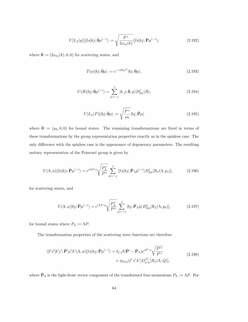
U [Lf (q)]|[ls]kj; 0µ(−)〉 :=

√P+

2ωm(k)|[ls]kj; Pµ(−)〉; (2.192)

where 0 := (2ωm(k), 0, 0) for scattering states, and

T (a)|bj; 0µ〉 := e−iMba0 |bj; 0µ〉, (2.193)

U(R)|bj; 0µ(−)〉 =

j∑

µ=−j

|b, j; 0, µ〉Djµµ(R), (2.194)

U [Lf (P )]|bj; 0µ〉 :=

√P+

µb|bj; Pµ〉 (2.195)

where 0 := (µb, 0, 0) for bound states. The remaining transformations are fixed in terms of

these transformations by the group representation properties exactly as in the spinless case. The

only difference with the spinless case is the appearance of degeneracy parameters. The resulting

unitary representation of the Poincare group is given by

U(Λ, a)|[ls]kj; Pµ(−)〉 = eiΛP ·a

√P+

Λ

P+

j∑

µ=−j

|[ls]kj; PΛµ(−)〉Dj

µµ[Rf (Λ, ps)], (2.196)

for scattering states, and

U(Λ, a)|bj; Pµ(−)〉 = eiΛP ·a

√P+

Λ

P+

j∑

µ=−j

|bj; PΛµ〉Djµµ[Rf (Λ, pb)], (2.197)

for bound states where PΛ := ΛP .

The transformation properties of the scattering wave functions are therefore

〈[l′s′]k′j′; P′µ′|U(Λ, a)|[ls]kj; Pµ(−)〉 = δj′jδ(P′ − PΛ)eiP ′·a

√P ′+

P+

× φklsj(l′ s′ k′)D(l)

µ′µ[Rf (Λ, Q)],

(2.198)

where PΛ is the light-front vector component of the transformed four-momentum PΛ := ΛP . For

64

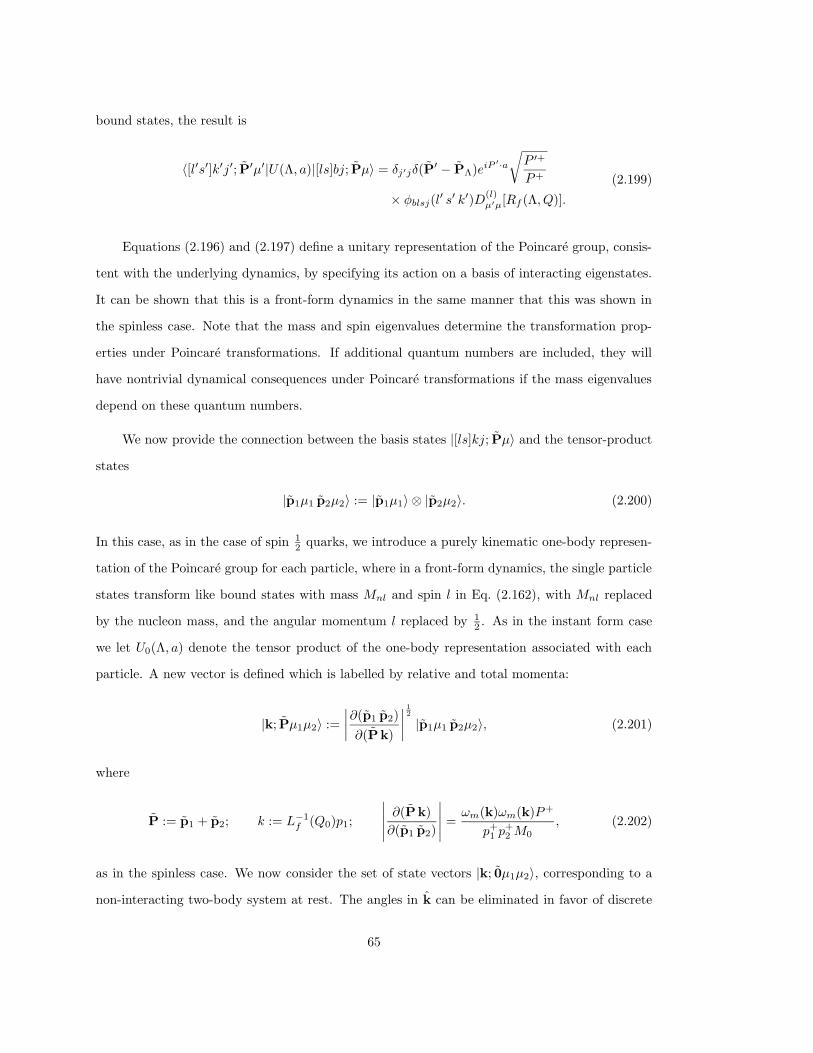
bound states, the result is

〈[l′s′]k′j′; P′µ′|U(Λ, a)|[ls]bj; Pµ〉 = δj′jδ(P′ − PΛ)eiP ′·a

√P ′+

P+

× φblsj(l′ s′ k′)D(l)

µ′µ[Rf (Λ, Q)].

(2.199)

Equations (2.196) and (2.197) define a unitary representation of the Poincare group, consis-

tent with the underlying dynamics, by specifying its action on a basis of interacting eigenstates.

It can be shown that this is a front-form dynamics in the same manner that this was shown in

the spinless case. Note that the mass and spin eigenvalues determine the transformation prop-

erties under Poincare transformations. If additional quantum numbers are included, they will

have nontrivial dynamical consequences under Poincare transformations if the mass eigenvalues

depend on these quantum numbers.

We now provide the connection between the basis states |[ls]kj; Pµ〉 and the tensor-product

states

|p1µ1 p2µ2〉 := |p1µ1〉 ⊗ |p2µ2〉. (2.200)

In this case, as in the case of spin 12 quarks, we introduce a purely kinematic one-body represen-

tation of the Poincare group for each particle, where in a front-form dynamics, the single particle

states transform like bound states with mass Mnl and spin l in Eq. (2.162), with Mnl replaced

by the nucleon mass, and the angular momentum l replaced by 12 . As in the instant form case

we let U0(Λ, a) denote the tensor product of the one-body representation associated with each

particle. A new vector is defined which is labelled by relative and total momenta:

|k; Pµ1µ2〉 :=

∣∣∣∣∂(p1 p2)

∂(P k)

∣∣∣∣12

|p1µ1 p2µ2〉, (2.201)

where

P := p1 + p2; k := L−1f (Q0)p1;

∣∣∣∣∣∂(P k)

∂(p1 p2)

∣∣∣∣∣ =ωm(k)ωm(k)P+

p+1 p

+2 M0

, (2.202)

as in the spinless case. We now consider the set of state vectors |k; 0µ1µ2〉, corresponding to a

non-interacting two-body system at rest. The angles in k can be eliminated in favor of discrete

65

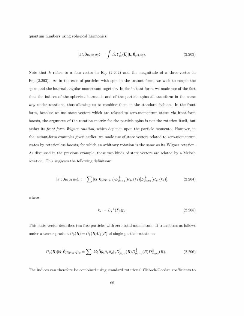
quantum numbers using spherical harmonics:

|kl; 0µlµ1µ2〉 :=

∫dkY l

µl(k)|k; 0µ1µ2〉. (2.203)

Note that k refers to a four-vector in Eq. (2.202) and the magnitude of a three-vector in

Eq. (2.203). As in the case of particles with spin in the instant form, we wish to couple the

spins and the internal angular momentum together. In the instant form, we made use of the fact

that the indices of the spherical harmonic and of the particle spins all transform in the same

way under rotations, thus allowing us to combine them in the standard fashion. In the front

form, because we use state vectors which are related to zero-momentum states via front-form

boosts, the argument of the rotation matrix for the particle spins is not the rotation itself, but

rather its front-form Wigner rotation, which depends upon the particle momenta. However, in

the instant-form examples given earlier, we made use of state vectors related to zero-momentum

states by rotationless boosts, for which an arbitrary rotation is the same as its Wigner rotation.

As discussed in the previous example, these two kinds of state vectors are related by a Melosh

rotation. This suggests the following definition:

|kl; 0µlµ1µ2〉c :=∑

|kl; 0µlµ1µ2〉D12µ1µ1

[Rfc(k1)]D12µ2µ2

[Rfc(k2)], (2.204)

where

ki := L−1f (P0)pi. (2.205)

This state vector describes two free particles with zero total momentum. It transforms as follows

under a tensor product U0(R) = U1(R)U2(R) of single-particle rotations:

U0(R)|kl; 0µlµ1µ2〉c =∑

|kl; 0µlµ1µ2〉cDlµlµl

(R)D12µ1µ1

(R)D12µ2µ2

(R). (2.206)

The indices can therefore be combined using standard rotational Clebsch-Gordan coefficients to

66

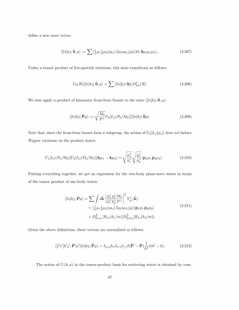
define a new state vector:

|[ls]kj; 0, µ〉 :=∑

〈 12µ1

12µ2|sµs〉〈lµlsµs|jµ〉|kl; 0µlµ1µ2〉c. (2.207)

Under a tensor product of free-particle rotations, this state transforms as follows:

U0(R)|[ls]kj; 0, µ〉 =∑

|[ls]kj; 0µ〉Djµµ(R). (2.208)

We now apply a product of kinematic front-form boosts to the state |[ls]kj; 0, µ〉:

|[ls]kj; Pµ〉 :=

√M0

P+U0[Lf (P0/M0)]|[ls]kj; 0µ〉. (2.209)

Note that, since the front-form boosts form a subgroup, the action of U0[Lf (pi)] does not induce

Wigner rotations on the product states:

U1[Lf (P0/M0)]U2[Lf (P0/M0)]|kµ1 − kµ2〉 =

√p+1

k+1

√p+2

k+2

|p1µ1 p2µ2〉. (2.210)

Putting everything together, we get an expression for the two-body plane-wave states in terms

of the tensor product of one-body states:

|[ls]kj; Pµ〉 =∑∫

dk

∣∣∣∣p+1 p

+2 M0

k+1 k

+2 P

+

∣∣∣∣

12

Y lµl

(k)

× 〈 12µ1

12µ2|sµs〉〈lµlsµs|jµ〉|p1µ1 p2µ2〉

×D12µ1µ1

[Rfc(k1/m)]D12µ2µ2

[Rfc(k2/m)].

(2.211)

Given the above definitions, these vectors are normalized as follows:

〈[l′s′]k′j′; P′µ′|[ls]kj; Pµ〉 = δµ′µδl′lδs′sδj′jδ(P′ − P)

1

k2δ(k′ − k). (2.212)

The action of U(Λ, a) in the tensor-product basis for scattering states is obtained by com-

67

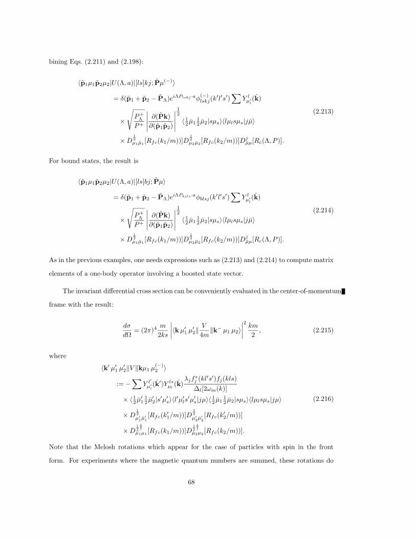
bining Eqs. (2.211) and (2.198):

〈p1µ1p2µ2|U(Λ, a)|[ls]kj; Pµ(−)〉

= δ(p1 + p2 − PΛ)eiΛPlskj ·aφ(−)lskj(k

′l′s′)∑

Y lµ′

l(k)

×

√P+

Λ

P+

∣∣∣∣∣∂(Pk)

∂(p1p2)

∣∣∣∣∣

12

〈 12 µ1

12 µ2|sµs〉〈lµlsµs|jµ〉

×D12µ1µ1

[Rfc(k1/m))]D12µ2µ2

[Rfc(k2/m))]Djµµ[Rc(Λ, P )].

(2.213)

For bound states, the result is

〈p1µ1p2µ2|U(Λ, a)|[ls]bj; Pµ〉

= δ(p1 + p2 − PΛ)eiΛPkjls·aφblsj(k′l′s′)

∑Y l

µ′

l(k)

×

√P+

Λ

P+

∣∣∣∣∣∂(Pk)

∂(p1p2)

∣∣∣∣∣

12

〈 12 µ1

12 µ2|sµs〉〈lµlsµs|jµ〉

×D12µ1µ1

[Rfc(k1/m))]D12µ2µ2

[Rfc(k2/m))]Djµµ[Rc(Λ, P )].

(2.214)

As in the previous examples, one needs expressions such as (2.213) and (2.214) to compute matrix

elements of a one-body operator involving a boosted state vector.

The invariant differential cross section can be conveniently evaluated in the center-of-momentum

frame with the result:

dσ

dΩ= (2π)4

m

2ks

∣∣∣∣〈kµ′1 µ′2‖

V

4m‖k− µ1 µ2〉

∣∣∣∣2km

2, (2.215)

where

〈k′ µ′1 µ′2‖V ‖kµ1 µ(−)2 〉

:= −∑

Y l′

µ′

l(k′)Y l∗

µl(k)

λjf∗j (kl′s′)fj(kls)

∆l[2ωm(k)]

× 〈 12 µ′1

12 µ′2|s′µ′s〉〈l′µ′ls′µ′s|jµ〉〈 1

2 µ112 µ2|sµs〉〈lµlsµs|jµ〉

×D12

µ′

1µ′

1[Rfc(k

′1/m))]D

12

µ′

2µ′

2[Rfc(k

′2/m))]

×D12†µ1µ1

[Rfc(k1/m))]D12†µ2µ2

[Rfc(k2/m))].

(2.216)

Note that the Melosh rotations which appear for the case of particles with spin in the front

form. For experiments where the magnetic quantum numbers are summed, these rotations do

68

not contribute to the cross section. For experiments where target and/or beam polarizations

are measured, the above formula can be used directly if one considers the spin rotations as a

change of representation. An important point is that the partial-wave representation of the

internal interaction is invariant. If V is given in a partial wave representation, then it can be

used to define a perturbation of M 20 which will provide the same fit to experimental data as a

nonrelativistic interaction V ′ = V/4m which has been fit to the same data.

69

2.7. Summary of Examples

We conclude this section with some general observations about the examples presented above.

We wish to stress again the difference between the dynamics contained in a model for the mass

operator M or its square, and the form of dynamics expressed in a particular unitary representa-

tion of the Poincare group. The eigenvalue equation which must be solved is identical in structure

to the Schrodinger equation, enabling us to make use of interactions fitted within a nonrelativistic

framework, but without sacrificing relativistic invariance. The choice of form then determines

the manner in which a system with four-momentum P is connected to the same system at rest.

It is at this point that relativity plays a role, and it is also clear that there are choices involved.

Different choices of forms of dynamics also affect the manner in which the spin labels of

state vectors are related under Lorentz transformations. In general, spin labels undergo Wigner

rotations under arbitrary Lorentz transformations. Canonical spins have the special property that

the Wigner rotation associated with a pure rotation is the rotation itself. This makes it possible

to combine spins of more than one particle with ordinary rotation Clebsch-Gordan coefficients.

Front-form spins can still be combined, but only after transforming to canonical spins with a

Melosh rotation. On the other hand, because the front-form boosts form a subgroup, front-form

spins do not undergo Wigner rotations under front-form boosts.

The interaction dependence of Lorentz transformations can be seen in the presence of the

mass eigenvalue in at least some of the transformations. The choice of form is also a choice as

to which subgroup of transformations does not depend upon the mass eigenvalue, but only on

free-particle kinematic variables. For instant-form dynamics, this subgroup includes rotations

and translations, but not boosts. In the front form, the subgroup involves certain combinations

of boosts and rotations. Transformations between two different forms of dynamics is relatively

straightforward when working with mass eigenstates. As stated above, the zero-momentum

eigenstates are independent of the form of dynamics. For non-zero momentum, they are related

by kinematic normalization factors and a Melosh rotation. Transformations between two different

forms of dynamics are considerably more complicated in a basis of single-particle product states,

because the mass operator is not diagonal in this basis.

70

3. Symmetries in Quantum Mechanics

In Sections 3–7, we present a more formal study of relativistic quantum mechanical models.

We begin in this section by examining the general requirements of Poincare invariance for a

quantum mechanical system. We then introduce infinitesimal generators and their commutation

relations, along with commuting Hermitian operators which are functions of the generators. The

corresponding treatment for systems satisfying Galilean invariance is also presented so that the

reader may better understand nonrelativistic systems within this context. In the relativistic case,

we pay particular attention to the spin operator, which has noticeably different features from the

nonrelativistic spin operator.

In quantum mechanics, symmetries imply constraints on the structure of a dynamical model.

In general, a symmetry transformation has the property that its action on a quantum mechanical

system leaves the physics unchanged. The predictions of quantum mechanics are probabilities.

A quantum mechanical symmetry transformation therefore has the property that its action on

states leaves probabilities unchanged. In a quantum theory, probabilities are expressed in terms

of a scalar product on the Hilbert space H. The probability of measuring a system prepared in

a state represented by |Ψ〉 to be found in a state represented by |Φ〉 is

PΨΦ :=|〈Ψ|Φ〉|2

〈Ψ|Ψ〉〈Φ|Φ〉 . (3.1)

A symmetry transformation is a correspondence of the form

|Ψ〉 → |Ψ′〉; |Φ〉 → |Φ′〉, (3.2)

which satisfies

PΨΦ = PΨ′Φ′ (3.3)

for all normalizable vectors |Ψ〉, |Φ〉 ∈ H. Wigner’s theorem (Go 66) shows that the most general

correspondence that preserves condition (3.3) is either a unitary or an antiunitary transformation

71

T :

|Ψ〉 → |Ψ′〉 = T (|Ψ〉) |Φ〉 → |Φ′〉 = T (|Φ〉). (3.4)

In the cases of Galilean invariance and Poincare invariance, there is an infinite number of

symmetry transformations that can be parameterized by elements of a continuous group G:

T → Tg g ∈ G. (3.5)

The group transformation properties require that

Tg2g1(|Ψ〉) and Tg2

(Tg1(|Ψ〉)) (3.6)

correspond to the same physical state. Because two normalized vectors that differ by an overall

phase correspond to the same physical state, the physical equivalence of the vectors in (3.6)

implies

Tg2(Tg1

(|Ψ〉)) = eiφ(g2,g1)Tg2g1(|Ψ〉), (3.7)

where the phase factor φ(g2, g1) depends on the group elements. This means that Tg is a “ray

representation” of G.

In the neighborhood of the identity, each group element is the square of another group

element:

Tg = Tg1 Tg1

(3.8)

(up to a possible phase factor), for g in a neighborhood of the identity. The composition of two

identical unitary or antiunitary transformations is unitary. Thus, Tg is unitary in the neighbor-

hood of the identity. If the group is pathwise connected, then all elements can be represented as

finite products of group elements in the neighborhood of the identity (A group is pathwise con-

nected if any two group elements can be continuously transformed from one to the other using a

group-valued curve γ(t), where 0 ≤ t ≤ 1 ). Since a finite product of unitary operators is unitary,

it follows that Tg is unitary for any g in the component of the group pathwise connected to the

identity.

72

Thus, for the component Tg of the Poincare group or Galilean group pathwise connected to

the identity, we write Tg → Ug, where Ug is unitary, and satisfies

Ug2Ug1

= eiφ(g1,g2)Ug2g1. (3.9)

A representation Ug satisfying Eq. (3.9) is called a unitary ray representation of the group G.

Because the assumption of invariant probabilities leads to a unitary symmetry, and unitary

operators preserve the eigenvalues of self-adjoint operators, it also follows that expectation values

and ensemble averages, which are composed of probabilities and eigenvalues, are also invariant.

This last statement requires a brief explanation with regard to tensor operators. For example,

consider the four-momentum, which transforms as a four-vector operator under the action of a

Lorentz transformation:

U(Λ, a)PµU(Λ, a)† = (Λ−1)µνP

ν . (3.10)

This equation appears to violate the above statement concerning invariance, since the components

of the momentum are not individually invariant.. That this is not the case can be seen by

considering the following:

Pµ|pµ〉 = pµ|pµ〉 → U(Λ, a)PµU(Λ, a)†U(λ, a)|pµ〉 = pµU(Λ, a)|pµ〉. (3.11)

From Eq. (3.11), we see that P ′µ := U(Λ, a)PµU(Λ, a)† and Pµ have identical eigenvalues corre-

sponding to different eigenvectors. In particular, the eigenvector of P ′µ with eigenvalue pµ is the

eigenvector of P µ with eigenvalue ΛµνP

ν . In making coordinate changes, both the states and

observables need to be transformed, and this results in identical expectation values. The same

result holds for ensemble averages.

73

3.1. Galilean Relativity

The Galilean principle of relativity (Ba 54, Le 63, Wa 70) states that the laws of quantum

mechanics do not distinguish between different inertial coordinate systems. This requires the

existence of a unitary ray representation of the group of transformations that relate different

inertial coordinate systems. What separates Galilean relativity from special relativity is the

assumed relation between different inertial coordinate systems. A system is consistent with the

principle of Galilean relativity if any two inertial coordinate systems are related by a coordinate

transform that preserves the form of Newton’s Second Law for a free particle.

The continuous transformations that preserve Newton’s Second Law for a free particle are

well known. They are generated by the following ten coordinate transformations:

(x, t) → (x′, t′) = (x, t+ t0); (3.12)

(x, t) → (x′, t′) = (x + a, t); (3.13)

(x, t) → (x′, t′) = (Rx, t), R ∈ SO(3); (3.14)

(x, t) → (x′, t′) = (x + vt, t), (3.15)

which represent time translations, space translations, rotations and Galilean boosts (uniform

rectilinear motion), respectively. These transformations generate the Galilean group of transfor-

mations, which has a linear representation by 5×5 matrices of the form (Wa 70):

g =

R v a

0 1 t0

0 0 1

, (3.16)

where R is a 3×3 rotation matrix, and v and a are real three-vectors. The matrix g acts on

column vectors that represent spacetime coordinates by

x =

x

t

1

→ x′ := gx =

Rx + vt+ a

t+ t0

1

. (3.17)

In this matrix representation, the 1 in the last row does not change when multiplied by the matrix

74

g. A Galilean invariant quantum theory requires that vectors corresponding to states in different

inertial coordinate systems are related by a unitary ray representation of the Galilean group:

|Ψ′〉 = Ug|Ψ〉, (3.18)

with Ug satisfying

Ug2Ug1

= eiφ(g2,g1)Ug2·g1. (3.19)

One of the complications of Galilean relativity is that the true representations (i.e., those where

the phase is not needed) do not have a reasonable physical interpretation (In 52). The problem

is that if one deduces the transformation properties of the infinitesimal generators of time trans-

lations (the Hamiltonian) and spatial translations (linear momentum) from the group structure,

they do not transform as would be expected in classical mechanics. To see this, consider a simul-

taneous eigenstate of the linear momentum operator and Hamiltonian (energy) |p, E〉. If U(v) is

the unitary representation of a Galilean boost U(x, t) is the unitary representation of a spacetime

translation, and Ug is a single valued unitary representation of the Galilean group, then the group

representation property (3.9) and the group multiplication law (Eqs. (3.12)–(3.15)) imply

U(x, t)U(v) = U(v)U(x− vt, t). (3.20)

We now apply U(x, t)U(v) to a simultaneous eigenstate |p;E〉 of energy and momentum, observ-

ing that

U(x, t)|p;E〉 = ei(p·x−Et)|p;E〉. (3.21)

The result is

U(x, t)U(v)|p;E〉 = U(v)U(x− vt, t)|p;E〉 = ei(p·x−(E+p·v)t)U(v)|p, E〉. (3.22)

We can read off the energy and momentum of the transformed state U(v)|p;E〉 as the coefficients

75

of t and x in the exponent:

E → E′ = E + p · v p → p′ = p. (3.23)

This differs from the expected transformation:

E → E′ = E + p · v +1

2mv2; p → p′ = p +mv. (3.24)

The difference between Eqs. (3.23) and (3.24) is contained in the terms proportional to the mass

m. By assuming a single valued representation, the terms involving the mass have been lost.

Bargmann (Ba 54) showed that the correct relations between energy and momentum are

recovered if one introduces a ray representation with the following phase factor:

φ(g1, g2) =m

2(aT

2 R2v1 − vT2 R1a1 + t1v

T2 R2v1), (3.25)

where the T superscript indicates the transpose of a vector. In this expression, m is the mass

of the particle. It is possible to treat Eq. (3.19) with the phase factor φ(g1, g2) using standard

group representation theory. This is done by extending the group to include a phase: g → (g, φ),

with the product:

(g1, φ1) (g2, φ2) = (g1 g2, φ1 + φ2 + φ(g1, g2)). (3.26)

The physical representation is not yet a true representation because of the usual phase ambiguity

associated with half-integral spin particles. This can be eliminated if the SO(3) group labels are

replaced by SU(2) labels. Given these two changes it is possible to realize the changes of inertial

coordinate systems as single valued unitary representations of the form

U(g2, φ2)U(g1, φ1) = U(g2 g1, φ21), (3.27)

where g → g denotes the replacement of the O(3) rotation R by an SU(2) rotation U and φ12

denotes the phase on the right hand side of (3.26). Technically, a unitary ray representation

of the Galilean group has been replaced by a single valued unitary representation of the central

76

extension (i.e., extending the group to include the phase factor φ(g1, g2)) of the universal covering

group (i.e., replacing SO(3) with SU(2)) of the Galilean group. Neither of these changes alters

the probabilities in Eq. (3.27). Their only effect is to allow the application of standard group

representation theory to the evaluation of such probabilities.

The central extension of the Galilean group is an eleven-parameter group. A unitary repre-

sentation has eleven infinitesimal Hermitian generators. These are the Hamiltonian H, which is

the infinitesimal generator of time translations; the linear momentum operators P, which are the

generators of spatial translations, the angular momentum operators J, which are the infinitesi-

mal generators of rotations, the operators K, which are the infinitesimal generators of uniform

rectilinear motion (Galilean boosts), and the mass M , which is the generator of phase trans-

formations in the central extension. The group transformation properties require that theses

generators satisfy certain commutation relations. The non-zero commutators are listed below:

[J i, Jk]−

= iεijkJk; [J i,Kk]−

= iεijkKk; [J i, P k]−

= iεijkP k (3.28)

[Kj , H]−

= −iP j ; [Kj , P k]−

= −iδjkM. (3.29)

There are two observations that can be made about these commutation relations that dis-

tinguish them from those of the Poincare group. The first is that in a Galilean invariant theory,

the mass operator is a generator. It commutes with all of the other generators. The second is

that the Hamiltonian never appears on the right-hand side of the non-vanishing commutators.

As will be seen shortly, this differs from a Poincare invariant theory, where the mass operator is

not a generator and the Hamiltonian appears on the right-hand side of some of the commutators.

The generator K is related to the position operator by

X := −K/M. (3.30)

An internal angular momentum or spin observable can also be defined in terms of these generators

77

by

j := J − X × P. (3.31)

The above analysis exhibits the operators normally used in nonrelativistic quantum mechan-

ics as functions of the infinitesimal generators associated with the underlying Galilean symmetry.

Before discussing Poincare invariance in quantum mechanics, it is instructive to consider the

constraints that Galilean invariance places on two-body interactions in nonrelativistic quantum

mechanics. These will be compared to similar constraints in the Poincare invariant case.

For a free particle, one can construct the generators of the Galilean group from the operators

M , P, j and X. For two free particles, the generators are sums of the one-body generators. The

position operator is then given by

X = −K1 + K2

M1 +M2=M1X1 +M2X2

M1 +M2, (3.32)

and the spin operator is

j = J − X × P = (j1 + X1 × P1 + j2 + X2 × P2) − X × (P1 + P2). (3.33)

It is possible to include an interaction V in the Hamiltonian in a manner that preserves the

commutation relations of the Galilean group without modifying any other generators. Since

H never appears on the right-hand side of any commutator, the commutation relations will be

satisfied if V commutes with the remaining generators. Equivalently, we can write

[P, V ]−

= [j, V ]−

= [X, V ]−

= [M,V ]−

= 0, (3.34)

since it is possible to construct the remaining generators as functions of these operators. These

conditions require that the interaction commutes with the total momentum, the total mass, is

independent of the total momentum, and is rotationally invariant. More general realizations are

possible if the other ten generators are allowed to have interactions, but these do not appear to

be of any practical interest.

78

3.2. Special Relativity - The Poincare group

In the case of the Poincare group, Bargmann showed that Wigner’s theorem could be modified

without loss of generality by replacing “ray representation of the component of the Poincare group

connected to the identity” by “single valued unitary representation of the covering group of the

Poincare group.” For completeness, the theorem is stated below (Ba 54):

A quantum mechanical model formulated on a Hilbert space preserves probabilities in all in-

ertial coordinate systems if and only if the correspondence between states in different inertial

coordinate systems can be realized by single valued unitary representation of the covering

group of the Poincare group.

This theorem will not be proved here, but the source of the difficulty is related phase ambi-

guities that occur when one rotates particles with half-integer spin through an angle of 2π. The

covering group does nothing more that put two distinct labels on each Lorentz transformation

that keeps track of these phases. The covering group of the Poincare group is inhomogeneous

SL(2, C), or ISL(2, C). Elements of the group are ordered pairs of 2×2 matrices (Λ, a), where Λ

has determinant = 1 and a is Hermitian. To understand the relation of ISL(2, C) to the Poincare

group, we note that any space-time coordinate xµ can be represented by a 2×2 Hermitian matrix:

X := xµσµ =

(x0 + x3 x1 − ix2

x1 + ix2 x0 − x3

); xµ = 1

2 Tr(σµX), (3.35)

where σ0 is the 2×2 identity matrix and σ are the three traceless Hermitian Pauli matrices,

σ0 :=

(1 0

0 1

); σ1 :=

(0 1

1 0

); σ2 :=

(0 −i

i 0

); σ3 :=

(1 0

0 −1

). (3.36)

In all that follows, an underscore will indicate a 2×2 matrix, except for the case of the Pauli ma-

trices, where we use the notation above. In this representation, the most general transformations

that preserve the proper time between events, the Hermiticity of X, the handedness of space and

the direction of time can be put in the form

X → X ′ = ΛXΛ† + a, (3.37)

with det|Λ|=1 and a = a†. These transformations preserve the proper time between events

79

because

τ2AB = det|XA −XB | = det|X ′A −X ′B | = τ2

A′B′ . (3.38)

Each of the pairs (Λ, a) and (−Λ, a) correspond to the same Poincare transformation satisfying

det|Λ| = 1 and Λ00 ≥ 1. From Eqs.(3.35)–(3.38), this correspondence is given by

Λµν := 1

2 Tr(σµΛσνΛ†); aµ = 12 Tr(σµa). (3.39)

The inverse expressions can be found in (Wi 60). In general, the notation Λµν , Λ, and Λ will be

used interchangeably. When there is any ambiguity, such as in the argument of a D function, the

2×2 matrix is the correct form to use. Similarly aµ, a and a will be used interchangeably. The

ordered pairs of matrices (Λ, a) form a group under composition

(Λ2, a2) (Λ1, a1) := (Λ2Λ1,Λ2a1Λ†2 + a2), (3.40)

with inverse

(Λ, a)−1 = (Λ−1,−Λ−1a(Λ†)−1). (3.41)

and identity (I, 0). The component of the Poincare group connected to the identity is isomorphic

to the group obtained by identifying (Λ, a) and (−Λ, a) in ISL(2, C). In the remainder of this

article, we use the notation P to denote ISL(2, C).

Inertial coordinate systems can be labeled by elements (Λ, a) of the Poincare group, or by

elements (Λ, a) of P . The difference is that P provides two distinct labels (Λ, a) and (−Λ, a) for

each inertial coordinate system, while elements of the component of the Poincare group connected

to the identity provide a unique label for each inertial coordinate system.

A single valued unitary representation U(Λ, a) of P is a function from the group P to the

space of linear operators on the model Hilbert space H satisfying:

U(Λ2, a2)U(Λ1, a1) = U [(Λ2, a2) (Λ1, a1)] = U(Λ2Λ1,Λ2a1(Λ2)† + a2), (3.42)

80

and

U(Λ, a)† = U(Λ, a)−1 = U [(Λ, a)−1]. (3.43)

The discussion to this point has identified a mathematical characterization of the concept of

relativistic invariance. The construction of a relativistic quantum mechanical model is equivalent

to construction of a unitary representation of the group P on the model Hilbert space. Below,

we will work out the consequences of the assumption that probabilities have values that are

independent of coordinate systems which are related by Poincare transformations.

3.3. Parameterization of Poincare Transformations

The group P is parameterized by an ordered pair (Λ, a) of 2×2 matrices, where the matrix

Λ is restricted to have det|Λ| = 1, and the matrix a is restricted to be Hermitian.

The most general 2×2 matrix Λ with det |Λ| = 1 can be represented by

Λ = Λ(θ,ρ) = exp(− i

2(θ + iρ) ·σ

). (3.44)

This follows because det | exp(C)| = exp(Tr(C)), and Tr(σ) = 0.

The parameters θ represent the angle and axis of a rotation, while ρ represents the direction

and rapidity of a rotationless Lorentz transformation. In general, unitary Λ’s represent rotations,

while positive Hermitian Λ’s represent rotationless Lorentz transformations. The polar decom-

position theorem ensures that any non-singular 2×2 matrix can be always be represented as the

product of a unitary matrix and a positive Hermitian matrix.

The most general 2×2 Hermitian matrix a has the form:

a = aµσµ, (3.45)

where the coefficients aµ are real. The parameters ρ, θ and aµ have the special property that if

any nine of them are set to zero, the subgroup generated by the remaining one is a one-parameter

Abelian subgroup. These quantities are taken as the ten parameters of P .

81

3.4. Definition of Infinitesimal Generators

Differentiation of the abstract representation U(Λ, a) with respect to angle, rapidity and

spacetime coordinate in the neighborhood of the identity defines abstract generators. Because

the representation U(Λ, a) is a one-parameter unitary Abelian group with respect to any of the

parameters ρ, θ or bµ with the other parameters set to zero, we can express U(Λ(θ,ρ), a) in the

form

U(Λ(θ,ρ), a) := eiP ·ae−i(J·θ+K·ρ) (3.46)

Note that the generators defined here sometimes have sign differences with generators defined

elsewhere. The source of this difference is in the sign of the generator of rotationless Lorentz

transformations. Our convention is fixed by Eq. (3.46) and the definition of rapidity in Eq. (3.44).

Equation (3.46) implies the following definitions for the infinitesimal generators:

Pµ := −igµν ∂

∂aνU(Λ, a)

∣∣∣∣ρ=θ=aµ=0

; (3.47)

Kj := i∂

∂ρjU(Λ, a)

∣∣∣∣ρ=θ=aµ=0

; (3.48)

Jj := i∂

∂θjU(Λ, a)

∣∣∣∣ρ=θ=aµ=0

. (3.49)

It follows from Stone’s theorem that these generators are self-adjoint operators (Yo 80). The

Hamiltonian H is the operator for the total energy of the system, which is the infinitesimal gen-

erator of time translations; P is the total linear momentum and J is the total angular momentum.

The generator K has no physical interpretation.

3.5. Commutation Relations - Canonical Form

The commutation relations of the generators defined in the previous subsection are computed

from the group representation property (3.42). These are given in three equivalent forms that are

useful in different applications. The commutation relations are needed to identify complete sets

of commuting self-adjoint operators, and to determine the spectrum of these operators. Given

82

these operators and a knowledge of their spectrum, it possible to construct representations of the

Hilbert space as a space of functions. This will be done in the next section.

The commutators of the generators can be computed from the definitions (3.47)–(3.49) and

the group representation property (3.42), using the formula:

∂2

∂c1∂c2

[U(g1)U(g2)U(g−1

1 )U(g−12 )]|ρ=θ=aµ=0

=∂2

∂c1∂c2U(g1 · g2 · g−1

1 · g−12 )|

ρ=θ=aµ=0

,

(3.50)

where gi = (Λi, ai), and g−1i = (Λ−1

i ,−Λ−1i ai(Λ

−1i )†), and ci are parameters chosen among ρi,

θi, and aµ.

These are most efficiently computed by using the infinitesimal forms and expanding in a

neighborhood of the identity to leading non-trivial order in the parameters ρi, θi and aµ. For ex-

ample, to compute the commutator ofK1 with J2, we use Eq. (3.46) to expand g1 = exp(− i2 iρ1σ1)

and g2 = exp(− i2θ2σ2) to first order in rapidity ρ1 and angle θ2 of the corresponding finite trans-

formations:

Λ1 = 1 − i

2iρ1σ1 + o(ρ2

1); Λ2 = 1 − i

2θ2σ2 + o(θ2

2). (3.51)

Keeping only the coefficients of ρ1θ2, we get

Λ1Λ2Λ−11 Λ−1

2

= I − 14ρ1θ2 [(iσ1)(σ2) + (iσ1)(−σ2) + (σ2)(−iσ1) + (−iσ1)(−σ2)] + · · ·

= I − i

2ρ1θ2(iσ3) + · · · .

(3.52)

On comparison with Eq. (3.46), we obtain

U(Λ1Λ2Λ−11 Λ−1

2 ) = U(I − i

2ρ1θ2(iσ3) + · · ·) = I − iρ1θ2K

3 + · · · . (3.53)

We also use Eq. (3.46) to expand U(g1) and U(g2) to first order in ρ1 and θ2:

U(Λ1, 0) = I − iρ1K1 + o(ρ2

1); U(Λ2, 0) = I − iθ2J2 + o(θ2

2), (3.54)

83

with the result:

U(Λ1)U(Λ2)U(Λ−11 )U(Λ−1

2 )

= I + ρ1θ2[(−iK1)(−iJ2) + (−iK1)(iJ2) + (−iJ2)(iK1) + (iK1)(iJ2)

]+ · · · .

(3.55)

Comparing the coefficients of ρ1θ2 in Eqs. (3.53) and Eq. (3.55) (or, equivalently, differentiating

and setting the parameters to zero), we get

[J2,K1]−

= J2K1 −K1J2 = −iK3. (3.56)

If this procedure is repeated for all pairs of generators, one obtains the following forty-five com-

mutators:

[Jj , Jk]−

= iεjklJ l; [Kj ,Kk]−

= −iεjklJ l; (3.57)

[Jj ,Kk]−

= iεjklKl; (3.58)

[Pµ, P ν ]−

= 0; (3.59)

[Kj , P 0]−

= −iP j ; [Jj , P 0]−

= 0; (3.60)

[Kk, P j ]−

= −iδjkP 0; [Jj , P k]−

= iεjklP l. (3.61)

Equations (3.57)–(3.58) are the commutation relations for the Lorentz group, Eqs. (3.59) give the

commutation relations for the group of spacetime translations, and Eqs. (3.60)-(3.61) constrain

Pµ to transform as a four-vector under Lorentz transformations.

Commutation Relations - Covariant Form The commutation relations can be put in a

84

manifestly covariant form if they are expressed in terms of the angular momentum tensor Jαβ :

J0j := Kj ; (3.62)

Jjk := εjklJ l; (3.63)

Jαβ := −Jβα. (3.64)

In terms of these operators, the commutation relations (3.57)-(3.61) become

[Jαβ , Jρσ]−

= i(gβσJαρ − gνρJασ + gαρJνσ − gασJνρ); (3.65)

[Pµ, P ν ]−

= 0; (3.66)

[Jρσ, Pµ]−

= i(gµρPσ − gµσP ρ). (3.67)

Commutation Relations - Front Form Any linear combinations of Poincare generators are

also generators. Another set of generators that is useful in applications is the set of “front-form”

generators. Since these generators are important in applications, we provide them explicitly.

They have the property that seven of them form a closed Lie subalgebra that does not involve

the generator that plays the role of the Hamiltonian. These are called “front form” generators

because the seven operators generate those Poincare transformations which leave the “light front”,

x+ := x0 + x3 = 0, invariant. If x+ is set to any non-zero constant, this surface is left invariant

by only a six-parameter subgroup. The seven generators are P 1 ,P 2, J3 and K3, which have

been defined previously, and

P+ := P 0 + P 3 (3.68)

E⊥ := K⊥ − z × J⊥. (3.69)

In addition to these, there are three other generators that take points on the light front to points

85

away from the light front:

P− := P 0 − P 3 (3.70)

F⊥ := K⊥ + z × J⊥. (3.71)

Sometimes F⊥ is replaced by J⊥. The operator P− plays the role of the Hamiltonian in the front

form, generating translations in x+. The finite Lorentz transformations generated by E1, E2, F 1

and F 2 correspond to one-parameter groups Λ(ρλ,θλ), with (θλ,ρλ) given by λ(x, y), λ(−y, x),

λ(−x, y) and λ(y, x), respectively. The commutation relations among the front-form generators

are fixed by the definitions (3.68)–(3.71). The commutation relations are given in Appendix B.

3.6. Commuting Self-Adjoint Operators

The generators H,P,J,K and the corresponding front-from generators can now be used

to construct a set of commuting self-adjoint operators. The eigenvalues of these operators are

used to label different irreducible representations of the Poincare group, and to label different

vectors in an irreducible subspace.

The Mass Operator The square of the mass operator is a second degree polynomial function

of the generators defined by

M2 := −PµPµ = H2 − P2 = P+P− − P2⊥. (3.72)

The commutation relations (3.57)–(3.61) imply that M 2 commutes with all of the operators

H,P,J,K and their front-form equivalents. If M 2 represents the mass of a real system, it is

a physical requirement that the eigenvalues of this operator are non-negative. Any self-adjoint

operator with strictly non-negative eigenvalues has a unique non-negative square root (Re 72).

Formally, this is the operator obtained by diagonalizing M 2 and replacing all of the eigenvalues

by their non-negative square roots. The mass operator associated with M 2 is defined by:

M :=√H2 − P2 =

√P+P− − P2

⊥. (3.73)

The mass operator is defined by this expression in any Poincare invariant quantum theory that

satisfies the spectral condition, M 2 ≥ 0. This is also true in local relativistic quantum field

86

theories, although the mass operator is seldom used in practice in field theories. The mass

operator commutes with all of the Poincare generators. For a single free particle, M has one

eigenvalue, which is the mass m. Relation (3.73) can also be used to express the Hamiltonian in

terms of the mass and the momentum operators:

H =√M2 + P2. (3.74)

The corresponding expression for P− is:

P− =M2 + P2

⊥P+

. (3.75)

The Pauli-Lubanski Operator In relativistic systems, the spin (total intrinsic angular mo-

mentum) is related to the Pauli-Lubanski vector (Lu 42), which is defined as follows:

Wµ := 12 ε

µαβγPαJβγ , (3.76)

where εµαβγ is the completely antisymmetric tensor in four dimensional spacetime with ε0123 = 1.

Wµ is a pseudo-four-vector, with components

W 0 = P · J; W = HJ − P× K. (3.77)

It follows from the commutation relations and the self-adjointness of the generators that

W 0 = (W 0)†; W = (W)†. (3.78)

From the commutation relations for the generators and Eqs. (3.77)–(3.78), it can also be shown

that Wµ has the following commutation relations with the generators

[Pµ,W ν ]−

= 0; (3.79)

[J,W 0]−

= 0; [Jj ,W k]−

= iεjklW l; (3.80)

[K,W 0]−

= −iW; [Kj ,W k]−

= −iδjkW 0. (3.81)

The relations (3.80) and (3.81) have the same form as Eqs. (3.60)–(3.61), with the generators

Pµ replaced by Wµ. These relations ensure that the components of W µ transform like a four-

87

vector under Lorentz transformations. The components of W µ have the following commutation

relations:

[Wµ,W ν ]−

= iεµνρσWρPσ. (3.82)

The quantity

W 2 := WµWµ := M2j2 (3.83)

is a polynomial in the generators that is independent of M 2 and commutes with all of the

generators. The operators W 2 and M2 are the only independent polynomial functions of the

generators that commute with all generators. The operator j2 is the total intrinsic spin operator

of the system.

Boosts Although the spin operator for the particle is unambiguously defined in terms of the

generators, there is an infinite number of spin vector valued functions of the generators that satisfy

angular momentum commutation relations and whose square is the total spin. The different types

of spin vectors are distinguished by their behavior under Lorentz boosts. To see this, note that

Eq. (3.76) implies the relation

WµPµ = 0. (3.84)

For timelike Pµ, Eq. (3.84) implies that the Pauli-Lubanski vector is spacelike. If P µ andWµ were

c-numbers, then Wµ could be transformed to a three-vector by a suitable Lorentz transformation.

Equation (3.83) implies that the resulting three-vector should be divided by M to obtain a spin

vector. The actual construction of a spin vector operator is more complicated, because relations

(3.79) and (3.84) are operator relations rather than c-number relations. In addition, there is more

than one way to transform a spacelike four-vector to a three-vector, since any rotation will not

change the three-vector nature of an operator.

We now construct a set of boost operators Lg(Q)µν , where Q := P/M is the four-velocity,

with the properties

Lg(Q)µν(1, 0, 0, 0)ν = M−1Pµ, (3.85)

88

and

Lg(1, 0, 0, 0)µ

ν = gµν . (3.86)

Equation (3.85) is to be interpreted as defining sixteen operator-valued functions of the operators

Pµ which, when applied to a simultaneous eigenstate of the operators P µ, take on the values

of the sixteen components of a Lorentz transformation that maps (m, 0, 0, 0) to P µ. This type

of Lorentz transformation will be called a “boost” which generalizes the notion of a rotationless

Lorentz transformation which will be referred to as a “canonical boost.” The index g differentiates

between different possible choices of Lorentz transformations that satisfy Eqs. (3.85) and (3.86).

Three different Lorentz transformations with this property are given below. These are known as

canonical (or rotationless) boosts, front-form boosts, and helicity boosts. These transformations

are used to construct the spin vectors which appear in most applications. The rotationless Lorentz

transformation L−1c (Q) was introduced in Section 2, and is defined by its action on a four-vector

Aµ:(A′0

A′

)= L−1

c (Q)

(A0

A

)=

(A0√

1 + Q2 − Q · A

A −A0Q + Q (Q · A)(1 +√

1 + Q2)−1

). (3.87)

The 2×2 matrix representation of this transformation is

Lc(Q) = exp( 12ω ·σ), (3.88)

where

ω := Q sinh−1Q, (3.89)

and Q := P/M and Q := |Q|. The inverse transformation of (3.87) is obtained by reversing the

sign of Q.

The front-form Lorentz boost Lf (Q), which was also introduced in Section 2, is defined by

the following action on any four-vector A:

A+′

A′⊥

A−′

= Lf (Q)

A+

A⊥

A−

=

Q+A+

A⊥ + Q⊥A+

(Q+)−1(Q2⊥A

+ + 2Q⊥ · A⊥ +A−)

, (3.90)

where A± := A0 ± A3. This is called a front-form boost because it is a type of Lorentz trans-

formation that leaves the light front (x+ = 0) invariant. The 2×2 matrix representation of this

89

transformation is:

Lf (Q) = exp

[1

2Q+(Q1 + iQ2)(σ1 − iσ2)

]exp( 1

2σ3 lnQ+)

= exp( 12σ3 lnQ+) exp

[12 (Q1 + iQ2)(σ1 − iσ2)

]

=1√Q+

(Q+ 0

(Q1 + iQ2) 1

).

(3.91)

The inverse transformation is obtained by the substitution Q⊥ → −Q⊥/Q+, Q+ → 1/Q+:

L−1f (Q) =

1√Q+

(1 0

−(Q1 + iQ2) Q+

). (3.92)

The third type of Lorentz transformation is associated with the helicity. The Lorentz trans-

formation Lh(Q) is a canonical boost in the z direction to a momentum of the desired magnitude,

followed by a rotation from the z axis to the axis that defines the direction of momentum (We

64):

Lh(Q) = R(z → p)Lc(|p|z), (3.93)

where the axis of rotation is

θ =z× P

|z × P| , (3.94)

and the angle of rotation is

θ = cos−1(z · P). (3.95)

Spin Vectors Each set of operators in the previous subsection has the property that when

their inverses are applied to a simultaneous eigenstate of P and M , they take on the value of a

Lorentz transformation that maps P µ to (M, 0, 0, 0). Since each of these operators is a function

of operators which in turn commute with all components of the Pauli-Lubanski vector, (see

Eq. (3.79)), it follows that

(0, jg) :=1

ML−1

g (Q)µνW

ν (3.96)

has three non-vanishing components when it is applied to any simultaneous eigenstate of P µ.

Note that although the right-hand side of (3.96) has the formal appearance of a four-vector,

90

and the left-hand side has the formal appearance of a three-vector, the quantity above does not

transform like a four-vector under Lorentz transformations, and does not generally transform like

a three-vector under rotations. This is because the argument of the Lorentz transformation is an

operator rather that a parameter. Only in the special case of the canonical spin does jc transform

like a three-vector under rotations. A subscript g has been included on jg to emphasize the fact

that different operators are obtained for different choices of Lg(Q)µν . The canonical spin jc, is

obtained from the canonical Lorentz boost, the front-form spin jf is obtained from the front-form

Lorentz transformation, and the helicity spin is obtained from the “helicity boost” Lh(Q). In

general, an infinite number of different types of spins is possible.

It is an immediate consequence of Eq. (3.96) and the transformation properties of four-vectors

under Lorentz transformations that

jg · jg =1

M2W 2 = j2 (3.97)

independent of g. Making use of the commutation relations among components of the Pauli-

Lubanski vector Wµ, we obtain

M2[jkg , j

lg] = iεklnM2jn

g (3.98)

for any choice of boost g. When M has no vanishing eigenvalues, the M 2 factor can be canceled

from both sides of this equation. The result is that any of the spin operators defined by Eq. (3.96)

satisfies SU(2) commutation relations:

[jkg , j

lg] = iεklnjn

g . (3.99)

Thus when M 6= 0, the spectrum of j2g is necessarily of the form s(s + 1), where s is an integer

or half integer. Similarly, the spectrum of any component of jg is (−s,−s+ 1, · · · , s− 1, s).

It is possible to extract the spin directly from the angular momentum tensor without explic-

itly constructing the Pauli-Lubanski vector. The components are given by

jkg = 1

2 εklnjln

g ; jlng := L−1

g (Q)lαL−1g (Q)n

βJαβ . (3.100)

Note that in the same way that jg is not a four-vector, the quantities jjkg are not the spatial

components of a tensor operator.

91

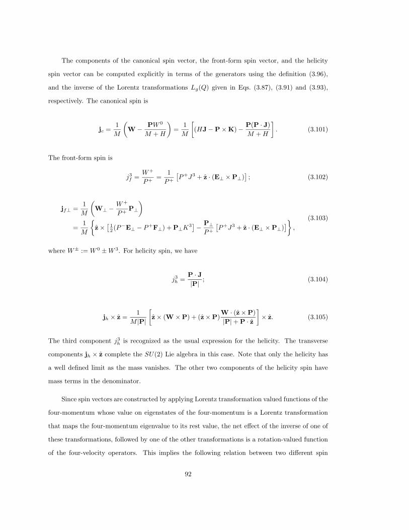
The components of the canonical spin vector, the front-form spin vector, and the helicity

spin vector can be computed explicitly in terms of the generators using the definition (3.96),

and the inverse of the Lorentz transformations Lg(Q) given in Eqs. (3.87), (3.91) and (3.93),

respectively. The canonical spin is

jc =1

M

(W − PW 0

M +H

)=

1

M

[(HJ − P× K) − P(P · J)

M +H

]. (3.101)

The front-form spin is

j3f =W+

P+=

1

P+

[P+J3 + z · (E⊥ × P⊥)

]; (3.102)

jf⊥ =1

M

(W⊥ − W+

P+P⊥

)

=1

M

z ×

[12 (P−E⊥ − P+F⊥) + P⊥K

3]− P⊥P+

[P+J3 + z · (E⊥ × P⊥)

],

(3.103)

where W± := W 0 ±W 3. For helicity spin, we have

j3h =P · J|P| ; (3.104)

jh × z =1

M |P|

[z × (W × P) + (z× P)

W · (z × P)

|P| + P · z

]× z. (3.105)

The third component j3h is recognized as the usual expression for the helicity. The transverse

components jh × z complete the SU(2) Lie algebra in this case. Note that only the helicity has

a well defined limit as the mass vanishes. The other two components of the helicity spin have

mass terms in the denominator.

Since spin vectors are constructed by applying Lorentz transformation valued functions of the

four-momentum whose value on eigenstates of the four-momentum is a Lorentz transformation

that maps the four-momentum eigenvalue to its rest value, the net effect of the inverse of one of

these transformations, followed by one of the other transformations is a rotation-valued function

of the four-velocity operators. This implies the following relation between two different spin

92

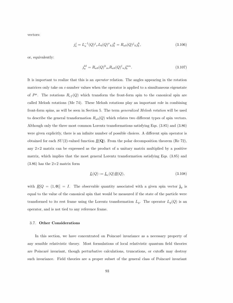
vectors:

jja = L−1

a (Q)jνLb(Q)ν

kjkb = Rab(Q)j

kjkb , (3.106)

or, equivalently:

jkla = Rab(Q)k

mRab(Q)lnj

mnb . (3.107)

It is important to realize that this is an operator relation. The angles appearing in the rotation

matrices only take on c-number values when the operator is applied to a simultaneous eigenstate

of Pµ. The rotations Rcf (Q) which transform the front-form spin to the canonical spin are

called Melosh rotations (Me 74). These Melosh rotations play an important role in combining

front-form spins, as will be seen in Section 5. The term generalized Melosh rotation will be used

to describe the general transformation Rab(Q) which relates two different types of spin vectors.

Although only the three most common Lorentz transformations satisfying Eqs. (3.85) and (3.86)

were given explicitly, there is an infinite number of possible choices. A different spin operator is

obtained for each SU(2)-valued function R(Q). From the polar decomposition theorem (Re 72),

any 2×2 matrix can be expressed as the product of a unitary matrix multiplied by a positive

matrix, which implies that the most general Lorentz transformation satisfying Eqs. (3.85) and

(3.86) has the 2×2 matrix form

L(Q) := Lc(Q)R(Q), (3.108)

with R[Q = (1,0)] = I. The observable quantity associated with a given spin vector jg is

equal to the value of the canonical spin that would be measured if the state of the particle were

transformed to its rest frame using the Lorentz transformation Lg. The operator Lg(Q) is an

operator, and is not tied to any reference frame.

3.7. Other Considerations

In this section, we have concentrated on Poincare invariance as a necessary property of

any sensible relativistic theory. Most formulations of local relativistic quantum field theories

are Poincare invariant, though perturbative calculations, truncations, or cutoffs may destroy

such invariance. Field theories are a proper subset of the general class of Poincare invariant

93

quantum models which are distinguished by the additional requirement of microscopic locality.

Microscopic locality means that there are observables associated with each bounded open subset

of space time, and that observables associated with any two causally disconnected subsets of

spacetime necessarily commute.

The principle of microscopic locality applies to observables associated with arbitrarily small

sets of spacetime, though any experimental test of this condition has only a finite resolution. In

an ideal scattering experiment, what is actually measured is the set of probability distributions of

momenta and spins of the initial and final particles at points which are asymptotically separated

from the spacetime volume in which the reaction occurs. We must therefore assume that the

dynamics permits states which behave asymptotically like systems of free particles. In quantum

field theory, this property is ensured by microscopic locality. However, in general, this condition

can be realized directly, by demanding that the dynamical model satisfy cluster separability prop-

erties or macroscopic locality. This is discussed in detail in Sections 6 and 7. Poincare invariant

models which replace microscopic locality with cluster properties cannot be distinguished from

local systems by any finite set of experiments.

94

4. The One-Body Problem: Irreducible Representations

The quantum mechanical description of a single particle of mass m and spin j is equivalent

to the construction of an irreducible representation of P with mass m and spin j. Irreducible

representations of P play a central role in all that follows. In addition to providing a mathe-

matical description of a single particle, they are used to formulate asymptotic conditions in the

mathematical description of scattering theory and cluster properties.

Consider a particle of mass m > 0 and spin j, with the property that transition probabilities

between different states of this particle are independent of the choice of inertial coordinate system.

From the discussion in Section 3, this is only possible if there exists an abstract representation

of P on the abstract one-particle Hilbert space H. Given this starting point, we develop a

mathematical description of this particle as follows:

1. Construct a complete set of commuting self-adjoint operators from the generators. Determine

the eigenvalue spectrum of the complete set of commuting self-adjoint operators in terms of

the mass and spin of the particle. Construct a representation of the model Hilbert space as

the space of square summable (integrable) functions of these eigenvalues.

2. Construct an explicit unitary representation of P on this representation of the Hilbert space

using transformation properties of the commuting operators.

3. Construct an explicit representation of the generators of P on this space.

4.1. The Hilbert Space

From the previous section, we know that the operators P, j3g ,M, j2 form a set of com-

muting self-adjoint operators that are constructed from the generators for any type (g) of spin.

The existence of these quantities as observable attributes of a particle is a consequence of the

assumption that one-body transition probabilities have values independent of inertial coordinate

system. The assumption of invariant transition probabilities ensures the existence of U(Λ, a)

by the Wigner-Bargmann theorem, that the infinitesimal generators are well defined functions

95

of U(Λ, a), and that the operators P, j3g ,M, j2 are well defined function of the infinitesimal

generators.

If the operators P, j3g ,M, j2 form a complete set of commuting self-adjoint operators, then

the particle will be called structureless. Since additional quantum numbers such as flavor, color,

charge, etc., play no special role in the description of the transformation properties of a free

particle under the action of the Poincare group, it is assumed in this section that the particle is

structureless.

The Hilbert space of any quantum mechanical system can be represented as the space of

square integrable functions of the eigenvalues of a complete set of self-adjoint operators. Thus,

the determination of the spectrum of the operators P, j3g ,M, j2 fixes a representation of the

model Hilbert space

The spectrum of these operators for a single particle of mass m and spin j is completely

determined by the specification of the mass and spin of the particle. The operator M has one

discrete eigenvalue which is m. The operator j2 also has only one discrete eigenvalue which is

j(j + 1). For particles with m > 0 the components of jg satisfy SU(2) commutation relations,

i.e., Eq. (3.99). This requires that j can take on only integral or half-integral values, and that

the spectrum of j3g can take the 2j + 1 values −j,−j + 1, . . . , j − 1, j. The spectrum of

the components of P range over the possible physical values of the momentum of the particle,

which is (−∞,∞). In a point-from or front-form description, the three components of the three-

momentum are replaced by three independent functions of the three-momentum. The spectrum

of these operators is determined by the range of these three independent functions as p varies

over its spectrum. These considerations completely determine the spectrum of the complete set

of commuting self-adjoint operators.

Of special interest are cases where the type of spin is canonical, front-form, or helicity, and

the continuous variables are the three components of the linear momentum, the three components

of the four-velocity, or the three components of the four-momentum that generate translations

that leave the light front invariant. Dirac’s three forms (Di 49) of the dynamics are associated

with specific combinations of spin and continuous variables. The natural commuting operators for

the instant form are the mass M , the linear momentum P, the spin j2 and the third component of

96

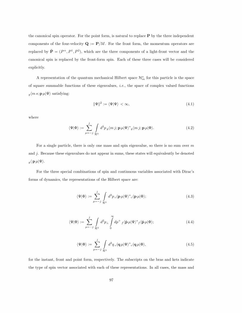
the canonical spin operator. For the point form, is natural to replace P by the three independent

components of the four-velocity Q := P/M . For the front form, the momentum operators are

replaced by P = (P+, P 1, P 2), which are the three components of a light-front vector and the

canonical spin is replaced by the front-form spin. Each of these three cases will be considered

explicitly.

A representation of the quantum mechanical Hilbert space Hsm for this particle is the space

of square summable functions of these eigenvalues, i.e., the space of complex valued functions

g〈ms;pµ|Ψ〉 satisfying:

‖Ψ‖2 := 〈Ψ|Ψ〉 <∞, (4.1)

where

〈Ψ|Φ〉 :=

j∑

µ=−j

∫

R3

d3p g〈mj;pµ|Ψ〉∗g〈mj;pµ|Φ〉. (4.2)

For a single particle, there is only one mass and spin eigenvalue, so there is no sum over m

and j. Because these eigenvalues do not appear in sums, these states will equivalently be denoted

g〈pµ|Ψ〉.

For the three special combinations of spin and continuous variables associated with Dirac’s

forms of dynamics, the representations of the Hilbert space are:

〈Ψ|Φ〉 :=

j∑

µ=−j

∫

R3

d3p c〈pµ|Ψ〉∗c〈pµ|Φ〉; (4.3)

〈Ψ|Φ〉 :=

j∑

µ=−j

∫

R2

d2p⊥

∞∫

0

dp+f 〈pµ|Ψ〉∗f 〈pµ|Φ〉; (4.4)

〈Ψ|Φ〉 :=

j∑

µ=−j

∫

R3

d3q c〈qµ|Ψ〉∗c〈qµ|Φ〉, (4.5)

for the instant, front and point form, respectively. The subscripts on the bras and kets indicate

the type of spin vector associated with each of these representations. In all cases, the mass and

97

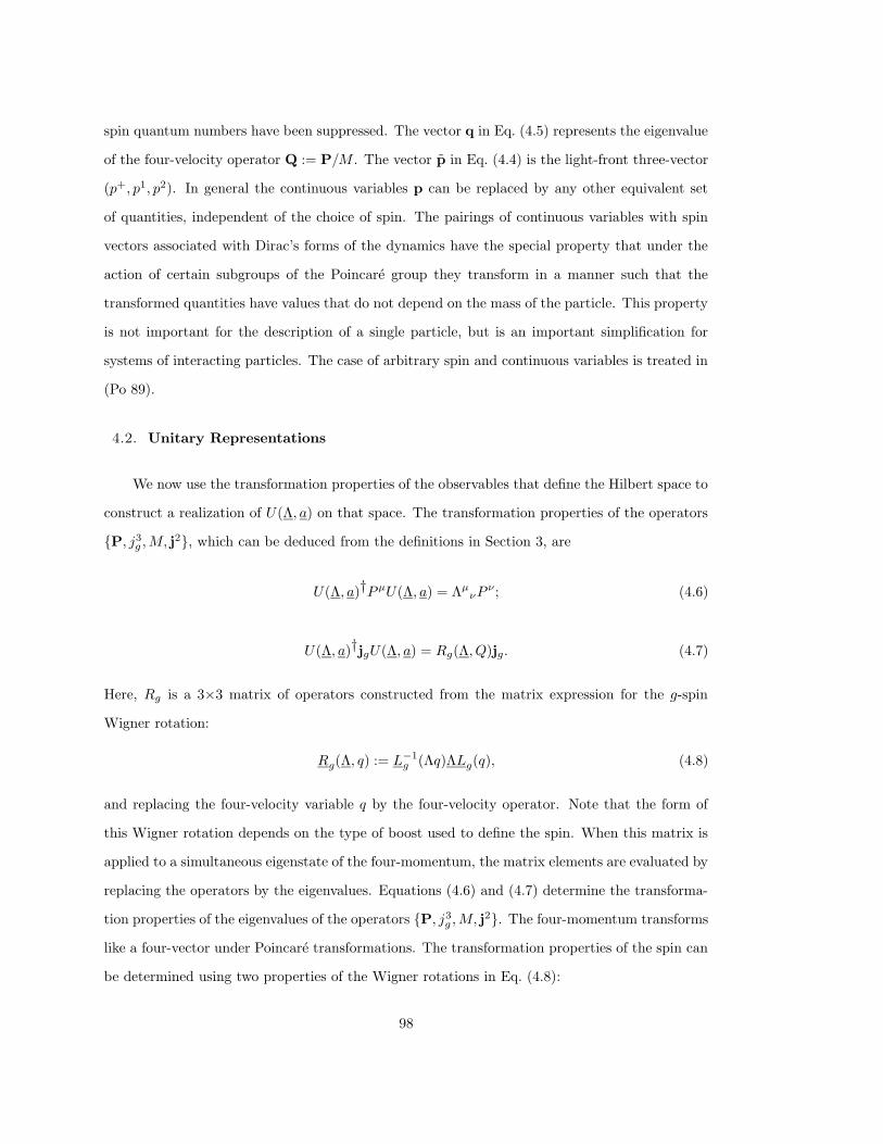
spin quantum numbers have been suppressed. The vector q in Eq. (4.5) represents the eigenvalue

of the four-velocity operator Q := P/M . The vector p in Eq. (4.4) is the light-front three-vector

(p+, p1, p2). In general the continuous variables p can be replaced by any other equivalent set

of quantities, independent of the choice of spin. The pairings of continuous variables with spin

vectors associated with Dirac’s forms of the dynamics have the special property that under the

action of certain subgroups of the Poincare group they transform in a manner such that the

transformed quantities have values that do not depend on the mass of the particle. This property

is not important for the description of a single particle, but is an important simplification for

systems of interacting particles. The case of arbitrary spin and continuous variables is treated in

(Po 89).

4.2. Unitary Representations

We now use the transformation properties of the observables that define the Hilbert space to

construct a realization of U(Λ, a) on that space. The transformation properties of the operators

P, j3g ,M, j2, which can be deduced from the definitions in Section 3, are

U(Λ, a)†PµU(Λ, a) = ΛµνP

ν ; (4.6)

U(Λ, a)†jgU(Λ, a) = Rg(Λ, Q)jg. (4.7)

Here, Rg is a 3×3 matrix of operators constructed from the matrix expression for the g-spin

Wigner rotation:

Rg(Λ, q) := L−1g (Λq)ΛLg(q), (4.8)

and replacing the four-velocity variable q by the four-velocity operator. Note that the form of

this Wigner rotation depends on the type of boost used to define the spin. When this matrix is

applied to a simultaneous eigenstate of the four-momentum, the matrix elements are evaluated by

replacing the operators by the eigenvalues. Equations (4.6) and (4.7) determine the transforma-

tion properties of the eigenvalues of the operators P, j3g ,M, j2. The four-momentum transforms

like a four-vector under Poincare transformations. The transformation properties of the spin can

be determined using two properties of the Wigner rotations in Eq. (4.8):

98

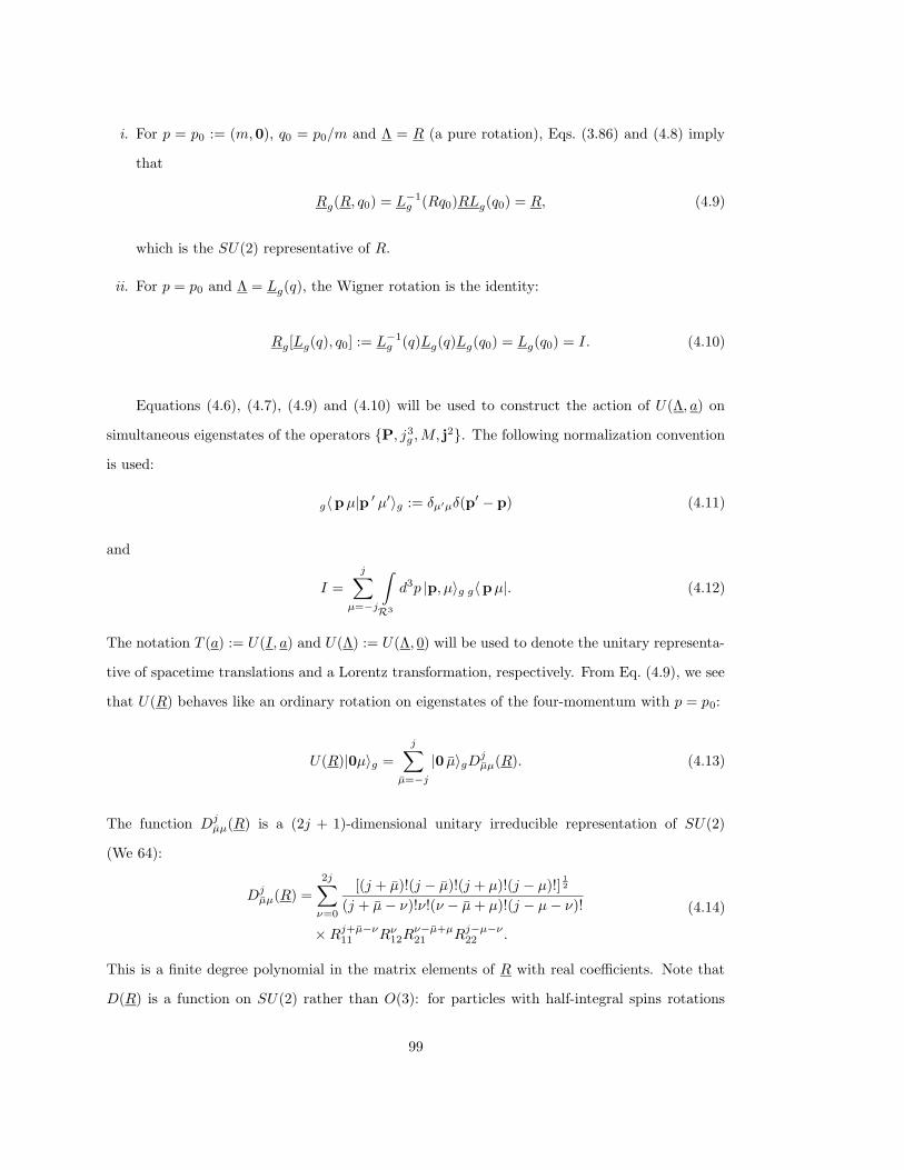
i. For p = p0 := (m,0), q0 = p0/m and Λ = R (a pure rotation), Eqs. (3.86) and (4.8) imply

that

Rg(R, q0) = L−1g (Rq0)RLg(q0) = R, (4.9)

which is the SU(2) representative of R.

ii. For p = p0 and Λ = Lg(q), the Wigner rotation is the identity:

Rg[Lg(q), q0] := L−1g (q)Lg(q)Lg(q0) = Lg(q0) = I. (4.10)

Equations (4.6), (4.7), (4.9) and (4.10) will be used to construct the action of U(Λ, a) on

simultaneous eigenstates of the operators P, j3g ,M, j2. The following normalization convention

is used:

g〈pµ|p ′ µ′〉g := δµ′µδ(p′ − p) (4.11)

and

I =

j∑

µ=−j

∫

R3

d3p |p, µ〉g g〈pµ|. (4.12)

The notation T (a) := U(I, a) and U(Λ) := U(Λ, 0) will be used to denote the unitary representa-

tive of spacetime translations and a Lorentz transformation, respectively. From Eq. (4.9), we see

that U(R) behaves like an ordinary rotation on eigenstates of the four-momentum with p = p0:

U(R)|0µ〉g =

j∑

µ=−j

|0 µ〉gDjµµ(R). (4.13)

The function Djµµ(R) is a (2j + 1)-dimensional unitary irreducible representation of SU(2)

(We 64):

Djµµ(R) =

2j∑

ν=0

[(j + µ)!(j − µ)!(j + µ)!(j − µ)!]12

(j + µ− ν)!ν!(ν − µ+ µ)!(j − µ− ν)!

×Rj+µ−ν11 Rν

12Rν−µ+µ21 Rj−µ−ν

22 .

(4.14)

This is a finite degree polynomial in the matrix elements of R with real coefficients. Note that

D(R) is a function on SU(2) rather than O(3): for particles with half-integral spins rotations

99

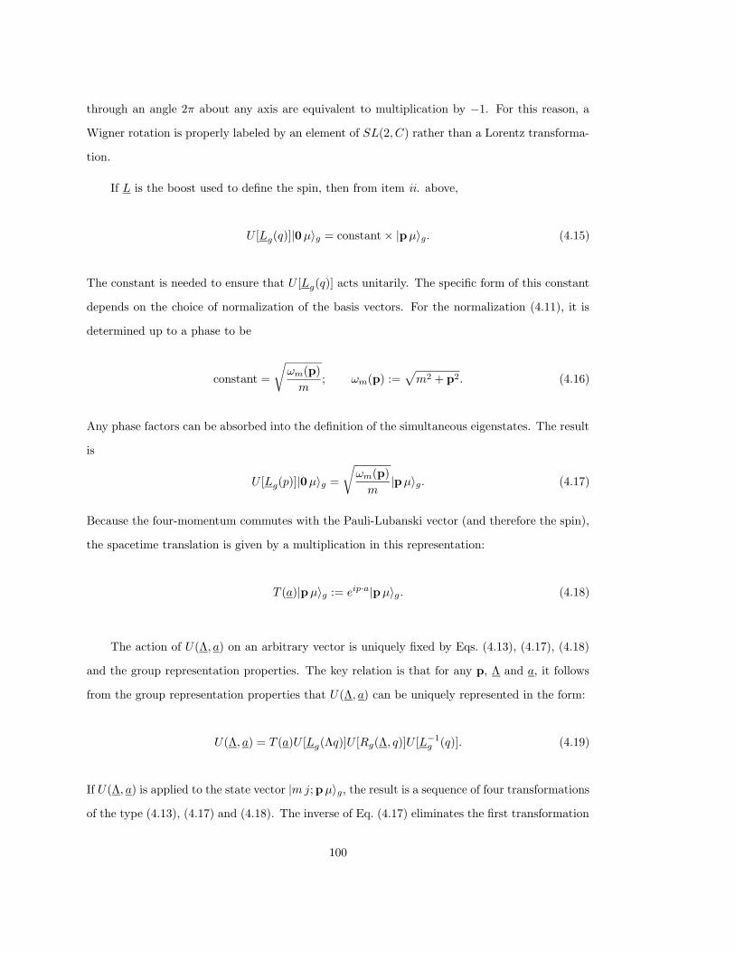
through an angle 2π about any axis are equivalent to multiplication by −1. For this reason, a

Wigner rotation is properly labeled by an element of SL(2, C) rather than a Lorentz transforma-

tion.

If L is the boost used to define the spin, then from item ii. above,

U [Lg(q)]|0µ〉g = constant × |pµ〉g. (4.15)

The constant is needed to ensure that U [Lg(q)] acts unitarily. The specific form of this constant

depends on the choice of normalization of the basis vectors. For the normalization (4.11), it is

determined up to a phase to be

constant =

√ωm(p)

m; ωm(p) :=

√m2 + p2. (4.16)

Any phase factors can be absorbed into the definition of the simultaneous eigenstates. The result

is

U [Lg(p)]|0µ〉g =

√ωm(p)

m|pµ〉g. (4.17)

Because the four-momentum commutes with the Pauli-Lubanski vector (and therefore the spin),

the spacetime translation is given by a multiplication in this representation:

T (a)|pµ〉g := eip·a|pµ〉g. (4.18)

The action of U(Λ, a) on an arbitrary vector is uniquely fixed by Eqs. (4.13), (4.17), (4.18)

and the group representation properties. The key relation is that for any p, Λ and a, it follows

from the group representation properties that U(Λ, a) can be uniquely represented in the form:

U(Λ, a) = T (a)U [Lg(Λq)]U [Rg(Λ, q)]U [L−1g (q)]. (4.19)

If U(Λ, a) is applied to the state vector |mj;pµ〉g, the result is a sequence of four transformations

of the type (4.13), (4.17) and (4.18). The inverse of Eq. (4.17) eliminates the first transformation

100

in Eq. (4.19):

T (a)U [Lg(Λq)]U [Rg(Λ, q)]

√m

ωm(p)|0µ〉g.

The new state vector is a rest state. From Eq. (4.13), the effect of the rotation is

√m

ωm(p)

j∑

µ=−j

T (a)U [Lg(Λq)]|mj;0 µ〉gDjµµ[Rg(Λ, q), ]

The rotated rest state can now be boosted using Eq. (4.17):

√ωm(pΛ)

m

√m

ωm(p)

j∑

µ=−j

T (a)|pΛ µ〉gDjµµ[Rg(Λ, q)].

Finally, Eq. (4.18) can be used to compute the action of the translation. The result is

U(Λ, a)|pµ〉g = eipΛ·a

√ωm(pΛ)

ωm(p)

j∑

µ=−j

|pΛ, µ〉gDjµµ[Rg(Λ, q)], (4.20)

where

pΛ := Λp; p = (ωm(p),p). (4.21)

Equation (4.20) is the key result of this section.

The operator U(Λ, a) is a single-valued unitary representation of P . Unitarity follows because

it can be expressed using Eq. (4.19) as the composition of four elementary unitary transforma-

tions. From Eq. (4.20), a wave function has the following transformation property:

g〈pµ|U(Λ, a)|Ψ〉 = eip·a

√ωm(pΛ−1)

ωm(p)

j∑

µ=−j

Djµµ[Rg(Λ, qΛ−1)]g 〈pΛ−1 µ|Ψ〉. (4.22)

The matrix elements of U(Λ, a) are

g〈p′ µ′|U(Λ, a)|pµ〉g = δ(p′ − pΛ)eip·a

√ωm(p′)ωm(p)

Djµ′µ[Rg(Λ, p)]. (4.23)

The above expressions give an explicit representation for U(Λ, a) on a basis of simultaneous

eigenstates of the three-momentum, the mass, and an arbitrary type of spin. These equations

101

are appropriate for Dirac’s instant form of dynamics if the spin is chosen to be the canonical spin

(g = c). In the point and front form of dynamics, the three components of the three-momentum

are replaced by three components of the four-velocity, or the front-form components of the four-

momentum, respectively. These choices have different natural normalizations for the continuum

variables, which require a different constant to maintain unitarity.

For the front form, the independent components of the momentum are replaced by

p → p := (p+, p1, p2), (4.24)

where p+ = ωm(p) + p3. The spin is taken to be the front-form spin and the normalization

condition is

f 〈p′ µ′|pµ〉f = δµ′µδ(p′+ − p+)δ2(p′⊥ − p⊥). (4.25)

For the front form, Eqs. (4.20), (4.22) and (4.23) are replaced as follows:

U(Λ, a)|pµ〉f = eipΛ·a

√p+Λ

p+

j∑

µ=−j

|pΛ µ〉fDjµµ[Rf (Λ, p)]; (4.26)

f 〈pµ|U(Λ, a)|Ψ〉 = eip·a

√p+Λ−1

p+

j∑

µ=−j

Djµµ[Rf (Λ, pΛ−1)]f 〈pΛ−1 µ|Ψ〉; (4.27)

f 〈p′ µ′|U(Λ, a)|pµ〉f = δ(p′ − pΛ)eip·a

√p′+

p+Dj

µ′µ[Rf (Λ, p)]. (4.28)

For the point form, let q := p/m, and use the basis

|qµ〉c = |ms;qµ〉c, (4.29)

with normalization

c〈q′ µ′|qµ〉c = δµ′µδ(q′ − q). (4.30)

102

Let qΛ := pΛ/m. With these conventions, Eqs. (4.20), (4.22) and (4.23) are replaced as follows:

U(Λ, a)|qµ〉c = eipΛ·a

√ω1(qΛ)

ω1(q)

j∑

µ=−j

|qΛ, µ〉cDjµµ[Rc(Λ, p)]; (4.31)

c〈qµ|U(Λ, a)|Ψ〉 = eip·a

√ω1(qΛ−1)

ω1(q)

j∑

µ=−j

Djµµ[Rc(Λ, pΛ−1)]c 〈qΛ−1 , µ|Ψ〉; (4.32)

g〈q′ µ′|U(Λ, a)|qµ〉c = δ(q′ − qΛ)eip·a

√ω1(q′)ω1(q)

Djµ′µ[Rc(Λ, p

′)]. (4.33)

The above equations define several concrete realizations of single-valued unitary representations

of P , corresponding to a single particle of mass m and spin j. This construction is the analog of

a plane wave basis for a single nonrelativistic particle. Although we have constructed a variety

of different unitary representations, they are all unitarily equivalent. The relations between

them can be deduced from the definitions. A more general basis of state vectors |gµ〉g can be

constructed, with g(p,m) representing any three independent functions of the three-momentum

(i.e., the front-form components, the three components of the four-velocity, or p itself). If there

are normalized in the usual way:

g〈g′ µ′|g µ〉g = δµ′µδ(g′ − g), (4.34)

then these states are related to the set |pµ〉t by a unitary transformation with coefficients

g〈g µ′|pµ〉t = δ(p − p(g;m))

∣∣∣∣∂p(g;m)

∂g

∣∣∣∣12

Djµ′µ[Rgt(p)]

= δ(g − g(p;m))

∣∣∣∣∂g(p;m)

∂p

∣∣∣∣12

Djµ′µ[Rgt(p)].

(4.35)

The transformations

Rgt(p) := L−1g (p)Lt(p) (4.36)

are the generalized Melosh rotations (Me 74) defined in Eqs. (3.106) and (3.107), which transform

between g and t type of spin. The square roots of the Jacobians maintain unitarity. The relevant

103

Jacobians relating p and q to p are

∣∣∣∣∂p(p;m)

∂p

∣∣∣∣ =p+

ωm(p);

∣∣∣∣∂q(p;m)

∂p

∣∣∣∣ =1

m3. (4.37)

4.3. Lie Algebra

Given representations of finite Poincare transformations in a given basis, it is possible to

construct representations of the Lie algebra in the same basis by differentiation using Eqs. (3.47)–

(3.49), along with the general formula (4.22) for the action of a unitary transformation on a wave

function. Representations of the Lie algebra are needed to derive constraints on model interactions

in the next section.

The generators of spacetime translations are multiplication operators:

P|mj;pµ〉g = p|mj;pµ〉g; (4.38)

H|mj;pµ〉g = ωm(p)|mj;pµ〉g. (4.39)

The formulas for the representations of the generators of Lorentz transformations depend on the

choice of spin. They are constructed from the definitions

g〈pµ|Kj |Ψ〉

:= i∂

∂ρj

j∑

µ=−j

∫

R3

d3p′ g〈pµ|U [Λ(θ,ρ)]|p′ µ〉g g〈p′ µ|Ψ〉

∣∣∣∣∣∣θ=ρ=0

;(4.40)

g〈p, µ|Jj |Ψ〉

:= i∂

∂θj

j∑

µ=−j

∫

R3

d3p′ g〈pµ|U [Λ(θ,ρ)]|p′ µ〉g g〈p′ µ|Ψ〉

∣∣∣∣∣∣θ=ρ=0

,(4.41)

where Λ(θ,ρ) is given by Eq. (3.44). If Eq. (4.22) is used in these relations and the result

differentiated, then the chain rule gives some factors and derivatives of the continuous variables.

104

The following result is obtained after performing the required differentiations:

Kj = −1

2ω(p), Xj

g+ + iCjkK (q)jk

g ; (4.42)

Jj = (Xg × p)j + CjkJ (q)jk

g , (4.43)

where Xjg := i(∂/∂pj) in the representation (4.22), and the matrices Cjk

J (q) and CjkK (q) are given

by

CjkK (q) := Cjk

1g (q) − q0Cjk2g (q); (4.44)

CjkJ (q) := Cjk

1g (q) + iεjlmClk2g(q)qm, (4.45)

where the coefficients Cjk1g (q) and Cjk

2g (q) are defined as follows:

Cjk1g (q) := 1

2Tr[L−1

g (q)σjLg(q)σk

](4.46)

Cjk2g (q) := Tr

[L−1

g (q)∂

∂qjLg(q)σk

]. (4.47)

For the case of canonical spin (Lg = Lc), a direct computation yields

K = −1

2ωm(p),Xc+ − 1

ωm(p) +m(p× jc); (4.48)

J = Xc × p + jc. (4.49)

For massive particles, (m + ω) is positive. Equation (4.49) has the form of the nonrelativistic

relation (3.33). It is clear from the general relation (4.43) for J that this connection is special

to canonical spin. Other types of spins are multiplied by a momentum dependent matrix that is

the identity only for p = 0 (by assumption (3.86)) . Thus, although all of the spins defined in

this paper coincide with the total angular momentum on states with p = 0, only the canonical

spin can be added to the orbital angular momentum with the usual rules of combining angular

momenta to obtain the total angular momenta. The canonical spin thus plays a special role in

relativistic dynamics.

105

The identification Xg = i∇p is also representation dependent. The operator Xg is repre-

sented by the derivative when the representation is irreducible and the spin is the g-spin. In these

cases, the partial derivative must be computed holding the degeneracy labels of the irreducible

representation constant. In representations where (m,p ) is replaced by (m,g ), such as the point

form or the front form, the operator Xg is represented by

Xjg =

∂gl

∂pjY l

g , (4.50)

where

Yg := i∇g. (4.51)

In the front form, the generators of front-form boosts play the same role as Xg. The general

case is treated in (Po 89). The operator Xg can be expressed directly in terms of the Poincare

generators by inverting Eq. (4.42) and replacing all eigenvalues by the corresponding operators:

Xjg = −1

2 1

H,Kj − iCjk

K (q)jkg +

, (4.52)

which is representation independent. For the case of canonical spin, this operator becomes

Xc = −1

2 1

H,K+ − P× (HJ − P × K)

MH(H +M). (4.53)

For massive particles, all of the inverted operators are bounded. The operator Xc is called

the Newton-Wigner position operator (Ne 49). Note that although all of the operators Xg are

derivatives with respect to p, up to normalization, this is true only in the representation in which

they are defined.

Equations (4.38), (4.39), (4.42) and (4.43) yield a representation for the Poincare Lie algebra

on the Hilbert space with normalization defined in Eq. (4.11). In order to construct the transverse

components of the spin operator, jg must be replaced by the appropriate linear combinations of

the raising and lowering operator for that spin.

106

In the instant form, the generators K and J are given explicitly by Eqs. (4.48) and (4.49),

respectively. In the point form, where the Hilbert space is represented by (4.30), the instant form

formulas can be used with the point form representation for X. In the front form, where the

Hilbert space is represented by states normalized according to Eq. (4.25), it is more convenient to

start from the finite transformations associated with E1, E2, andK3. These finite transformations

leave the three-component of the front-form spin invariant. In the front-form representation, these

three operators are:

Ei = −ip+ ∂

∂pi; (4.54)

K3 = −ip+ ∂

∂p+. (4.55)

From these representations, it is possible to construct a representation of the Lie algebra. The

spacetime translation generators are simply multiplication operators:

P+ = p+; P i = pi (i = 1, 2); P− =m2 + p2

⊥p+

:= p−, (4.56)

while the remaining Lorentz generators can be expressed in terms of these operators and the

front-form spin operators by inverting Eqs. (3.102)–(3.103):

J3 = j3f − z

P+· (P× E); (4.57)

F⊥ = 2P⊥z · KP+

+P−

P+E⊥ +

2

P+z × [P⊥(z · jf ) +M jf⊥]. (4.58)

It is sometimes customary to use the transverse components of the total angular momentum

to replace F⊥. These operators have the form

J⊥ =1

P+

[12 (P+ − P−)(z× E⊥) − (z× P⊥)K3 + P⊥ j

3f +M jf⊥

]. (4.59)

107

4.4. Position in Relativity

Our development of relativistic quantum mechanics has been done in a momentum repre-

sentation. This is because the four-momentum operators arise naturally in a relativistic model

as the infinitesimal generators of spacetime translations. It is no accident that we have not made

a parallel development in configuration space. The problem is that there is no suitable position

observable in relativistic quantum mechanics. The most conventional approach is a field theoretic

argument that follows from the uncertainty principle: if one attempts to localize the position of

a particle of mass m in a region of dimension ∆x, then one must use a probe with momentum

transfer greater than ∆p = h/∆x. When ∆p is of order m, it is possible to add enough energy

to the system to create a particle identical to the one whose position is being localized. Since the

newly created particle cannot be distinguished from the original, we find the following limitation:

∆x ≥ h/m, which is the Compton wavelength of the particle.

This argument is based on the assumption that the model allows particle production. It is

possible to show that difficulties occur in defining a position operator, whether the model admits

particle production or not. The argument below is due to Haag (Ha 00, Sc 61).

We begin by considering the form of the wave function of a spinless particle at the origin at

time t = 0. Let us denote the wave function of this particle by 〈p|x = 0; t = 0〉. If such a state

is invariant under homogeneous Lorentz transformations, then

〈p|x = 0; t = 0〉 = 〈p|U(Λ)|x = 0; t = 0〉 =

√ωm(pΛ−1)

ωm(p)〈pΛ−1 |x = 0; t = 0〉. (4.60)

The wave function 〈p|x = 0; t = 0〉 must therefore have the form

〈p|x = 0; t = 0〉 =1√

ωm(p)f(p2) =

1√ωm(p)

f(m2) =C√ωm(p)

, (4.61)

where C is constant. We can now translate this eigenstate to construct an eigenstate correspond-

ing to a particle localized at x:

〈p|x; t = 0〉 = 〈p|T (x)|x = 0; t = 0〉 = e−ip·x C√ωm(p)

. (4.62)

If we take the overlap between the state at (x = 0; t = 0) with a state at (x 6= 0; t = 0), the result

108

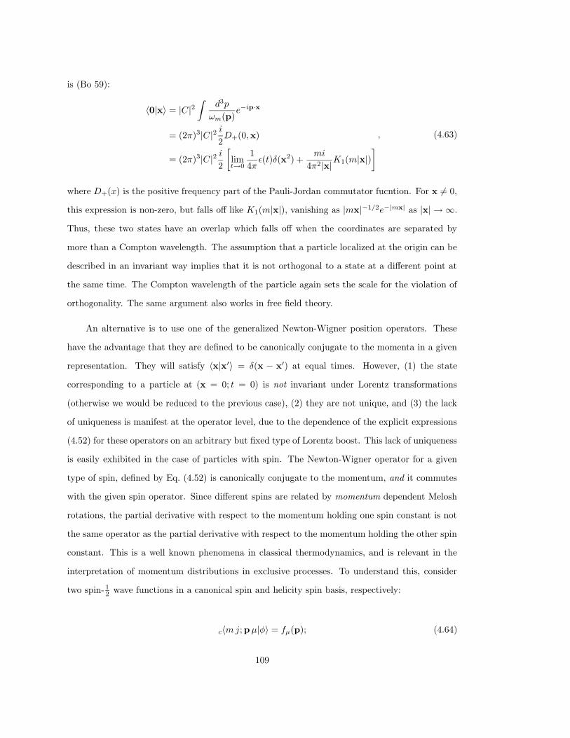
is (Bo 59):

〈0|x〉 = |C|2∫

d3p

ωm(p)e−ip·x

= (2π)3|C|2 i2D+(0,x)

= (2π)3|C|2 i2

[limt→0

1

4πε(t)δ(x2) +

mi

4π2|x|K1(m|x|)], (4.63)

where D+(x) is the positive frequency part of the Pauli-Jordan commutator fucntion. For x 6= 0,

this expression is non-zero, but falls off like K1(m|x|), vanishing as |mx|−1/2e−|mx| as |x| → ∞.

Thus, these two states have an overlap which falls off when the coordinates are separated by

more than a Compton wavelength. The assumption that a particle localized at the origin can be

described in an invariant way implies that it is not orthogonal to a state at a different point at

the same time. The Compton wavelength of the particle again sets the scale for the violation of

orthogonality. The same argument also works in free field theory.

An alternative is to use one of the generalized Newton-Wigner position operators. These

have the advantage that they are defined to be canonically conjugate to the momenta in a given

representation. They will satisfy 〈x|x′〉 = δ(x − x′) at equal times. However, (1) the state

corresponding to a particle at (x = 0; t = 0) is not invariant under Lorentz transformations

(otherwise we would be reduced to the previous case), (2) they are not unique, and (3) the lack

of uniqueness is manifest at the operator level, due to the dependence of the explicit expressions

(4.52) for these operators on an arbitrary but fixed type of Lorentz boost. This lack of uniqueness

is easily exhibited in the case of particles with spin. The Newton-Wigner operator for a given

type of spin, defined by Eq. (4.52) is canonically conjugate to the momentum, and it commutes

with the given spin operator. Since different spins are related by momentum dependent Melosh

rotations, the partial derivative with respect to the momentum holding one spin constant is not

the same operator as the partial derivative with respect to the momentum holding the other spin

constant. This is a well known phenomena in classical thermodynamics, and is relevant in the

interpretation of momentum distributions in exclusive processes. To understand this, consider

two spin- 12 wave functions in a canonical spin and helicity spin basis, respectively:

c〈mj;pµ|φ〉 = fµ(p); (4.64)

109

h〈mj;pµ|ψ〉 = fµ(p). (4.65)

The wave function fµ(p) is chosen to be the same in each case, although the representations

are different. In both expressions, p is the three-momentum. The Fourier transforms of each

of these wave functions are clearly the same. On the other hand, if we take the wave function

c〈ms;pµ|φ〉, and perform the unitary transformation that puts it into the same representation

as the wave function h〈ms;pµ|ψ〉, then the new wave function is

fµ(p) → f ′µ(p) =∑

µ

D12µµ[Rhc(p/m)]fµ(p). (4.66)

If we Fourier transform f ′µ(p), which is fµ(p) in the representation (4.65), it will have different x

dependence than the Fourier transform of fµ(p) in the representation (4.64). Thus, the x depen-

dence for a given momentum distribution is different depending on the choice of spin observable.

Because the generalized Melosh rotation is irrelevant when we sum over magnetic quantum num-

bers, this difficulty will be most apparent if one attempts to make spacetime interpretations of

processes where spin degrees of freedom are measured.

The conclusion is that although configuration space wave functions can be used as well

as momentum space wave functions, one should never attempt to interpret the coordinates as

observable quantities, especially on distance scales on the order of a Compton wavelength of

a particle. We note that the concept of position gets even more complicated in models with

interactions (Fo 64).

4.5. Summary

This completes the discussion of the description of a single relativistic particle of mass m

and spin j. The starting point was the assumption that there exists an abstract unitary represen-

tation of P0 on an abstract Hilbert space. Abstract expressions for the infinitesimal generators

were then developed, and their commutation relations were determined. The generators were

used to construct a complete set of commuting Hermitian operators, including the mass and

spin. The spectrum of the complete set of commuting self-adjoint operators was determined,

and representations of the model Hilbert space were constructed as spaces of square-integrable

110

functions of the eigenvalues of these operators. The condition of unitarity and a knowledge of

how the operators behave under finite Poincare transformations led to unitary representations

of P0 on the these Hilbert spaces. Finally, formal differentiation of these unitary operators with

respect to parameters of the Poincare group led to representations of the infinitesimal generators.

The only point where the assumption was made that this space describes a single particle

was in the specification of the spectrum of the mass and spin operators. A similar analysis applies

to systems of noninteracting particles. The construction of a representation of the Hilbert space

is the same, except the spectrum of the mass and spin operators is richer.

The transformations and spaces constructed in this section define irredcuible representations

of the Poincare group. All of the results of this section extend immediately to systems of particles,

provided the representaions are first reduced to superpositions of irreducible represenations. From

a mathematical point of view, there are additional classes of irreducible representations of P

(Mo 65). The representations discussed in this section are appropriate to particles with positive

real mass and positive energy.

111

5. The Two-Body Problem

As shown in the previous section, irreducible representations of the Poincare group are

characterized by a mass m and spin j. As far as the representation is concerned, it does not

matter whether the physical object described is in any sense ‘elementary’ or composite, nor does

such an irreducible representation depend upon any dynamical theory behind it, once the mass

and spin are specified. It is only at the level of the two-body problem that dynamics can be

specified in distinguishable ways. In this section, the Bakamjian-Thomas construction for two

interacting particles is developed in detail, using results from the previous section on the one-body

problem. The construction proceeds as follows:

1. The two-particle Hilbert space is defined as the tensor product of two one-particle Hilbert

spaces.

2. A two-body unitary representation of P on the two-particle Hilbert space is defined as the

tensor product of two one-body representations. In general, this representation is reducible.

3. Clebsch-Gordan coefficients for the Poincare group are constructed and used to reduce the

unitary representation of P on the two-particle Hilbert space to a linear superposition (direct

integral) of irreducible representations of P .

4. Poincare generators for irreducible representations of the non-interacting two-particle system

are constructed, along with operators for the mass and spin, and the generalized Newton-

Wigner position operators.

5. Following Bakamjian and Thomas, interactions are added to the mass operator in the irre-

ducible free-particle representation, which, together with the non-interacting spin and gen-

eralized Newton-Wigner position operators, are used to construct Poincare generators for

the interacting system. These generators are used to construct a new unitary representation

of P with interactions.

6. Special choices of the Clebsch-Gordan coefficients in Step 3 yield two-body models associated

with Dirac’s different forms of dynamics. These are discussed and related.

112

The methods presented are sufficiently flexible to permit the formulation of models consistent

with existing two-body scattering data and spectral properties.

5.1. The Two-Body Hilbert Space

The Hilbert space H(2) for a system of two particles of mass mi and spin si (i = 1, 2) is the

tensor product, Hs1m1

⊗ Hs2m2

, of the single-particle Hilbert spaces associated with each particle.

A basis on this space can be constructed from single-particle bases:

|p1 µ1 p2 µ2〉g := |m1 s1;p1 µ1〉g ⊗ |m2 s2;p2 µ2〉g, (5.1)

with normalization

g〈p′1 µ′1 p′2 µ′2|p1 µ1 p2 µ2〉g = δµ′

1µ1δµ′

2µ2δ(p′1 − p1 )δ(p′2 − p2 ). (5.2)

The subscript g denotes the type of boost used to define the spin.

5.2. Relativistic Dynamics of Two Free Particles

The unitary representation U0(Λ, a) of P for two free particles is the tensor product of two

single-particle representations:

U0(Λ, a) := U1(Λ, a) ⊗ U2(Λ, a). (5.3)

In this representation, the Poincare generators are sums of the generators for each particle:

Pµ0 := Pµ

1 ⊗ I2 + I1 ⊗ Pµ2 ; (5.4)

K0 := K1 ⊗ I2 + I1 ⊗ K2; (5.5)

J0 := J1 ⊗ I2 + I1 ⊗ J2. (5.6)

Equations (5.5) and (5.6) can be replaced by the covariant relation:

Jαβ0 := Jαβ

1 ⊗ I2 + I1 ⊗ Jαβ2 . (5.7)

The single-particle generators are given in Section 4, and the operator Ii is the identity operator on

113

Hsimi

. The zero subscript on the generators indicates that they correspond to the non-interacting

system.

The front-form generators for two free particles, P+0 , P−0 , P0⊥, E0⊥, K3

0 , J30 and F0⊥ are

obtained by taking the linear combinations of the generators defined in Eqs. (3.68)–(3.71).

Operators corresponding to the total mass and spin for the non-interacting system can be

constructed from these generators using the definitions in Section 3. Since the mass and spins

are nonlinear functions of the two-body generators, they cannot be represented as sums of single-

particle operators.

5.3. Clebsch-Gordan Coefficients

In nonrelativistic quantum mechanics, both translational invariance and rotational invariance

of the system lead to simplifications of the dynamical equations if the mass and spin of the

combined system are used as variables in the dynamical equations. A similar simplification occurs

in relativistic quantum mechanics. In the latter case, this involves a change of representation, in

which the single-particle momenta and spins are replaced by an overall system momentum and

internal angular momentum. Mathematically, the two-particle basis (5.1) is a tensor product

of irreducible representation spaces of P . The problem of changing to a basis in which the

variables are the total four-momentum and the spin is mathematically equivalent to the problem

of constructing Clebsch-Gordan coefficients for the Poincare group. These are coefficients of the

unitary transformation that reduces a tensor product of two irreducible representations of P to

a linear superposition (direct integral) of irreducible representations of P . The resulting basis

still describes a system of free particles. Working with irreducible representation is central to

the Bakamjian-Thomas method for adding interactions used in this paper. Although expressions

for the Clebsch-Gordan coefficients can be found in the literature (Mo 65), their explicit form

depends on normalization conventions and spin conventions. They can be constructed in a

straightforward manner. We consider several different cases corresponding to different choices of

spin and continuous variables.

The problem of constructing the Clebsch-Gordan coefficients of the Poincare group is equiv-

alent to the problem of expressing products of single-particle eigenstates as linear combinations

114

of two-body states that have the same transformation properties as a free particle. A particle of

mass m and spin j is characterized by a timelike four-momentum with rest energy m, and with

rest eigenstates which transform as a spin-j irreducible representation under rotations, i.e.,

U(R)|mj;0µ〉 =∑

µ

|mj;0 µ〉Djµ,µ(R). (5.8)

The construction presented below corresponds to the special case that both representations cor-

respond to massive physical particles. Treatments of general representations can be found in the

original papers of Wigner (Wi 39) and Bargmann (Ba 47), and also from a more modern point

of view in Mackey’s theory of induced representations (Ma 66).

The goal of the construction of the Clebsch-Gordan coefficient is to express the tensor-

product states (5.1) as linear combinations of eigenstates of the total four-momentum, with the

property that the rest eigenstates transform as spin-j irreducible representation under rotations.

The first step in the construction of the Clebsch-Gordan coefficients is to identify eigenstates

of the four-momentum. From Eq. (5.4), it follows that the four-momentum of the non-interacting

two-body system is the sum of the four-momenta of each constituent particle. Since for massive

particles the individual four-momenta are timelike, it follows that the total four-momentum is a

timelike four-vector. It is always possible to find a Lorentz boost that transforms a state with a

timelike four-momentum to a rest state.

The fundamental observation is that the rest four-momentum is invariant under rotations

and spacetime translations. For each fixed mass, the spacetime translations of the rest eigenstates

are given by multiplication by a phase which is independent of any internal degrees of freedom of

the rest eigenstate. In general, the internal degrees of freedom transform among themselves non-

trivially under the action of rotations. The next step is to express the rest eigenstate as a linear

combination of terms, each of which transforms irreducibly under rotations. Rest eigenstates

with different spins can be boosted to yield a direct sum of irreducible representation of the

Poincare group for a given mass. The desired linear superposition or direct integral is obtained

by including the contribution of these direct sums for each mass. The Clebsch-Gordan coefficients

can be read off once the normalization of these combined states are fixed.

115

We begin with the problem of coupling two-particle states with canonical spin to a superpo-

sition of states with canonical spin. The four-momentum of a tensor product state,

Pµ|p1 µ1 p2 µ2〉c = (pµ1 + pµ

2 )|p1 µ1 p2 µ2〉c, (5.9)

is the sum of the four-momenta of each particle. This is related to a rest eigenstate by the inverse

canonical boost with the four-velocity associated with this four-momentum. In what follows, it

is more convenient to label the arguments of boost and Wigner rotation by four-momenta rather

than four-velocities. Thus, Lc(P ) will be used interchangeably with Lc(Q) := Lc(P/√−P 2), and

similarly for Wigner rotations. This rest eigenstate is defined as follows:

√ωm1

(p1)ωm2(p2)

ωm1(k)ωm2

(k)U(L−1

c (P ))∑

|p1 µ1 p2 µ2〉c

×Dj1µ1µ1

[R−1c (L−1

c (P ), p1)]Dj2µ2µ2

[R−1c (L−1

c (P ), p2)].

(5.10)

This is an eigenstate of the four-momentum with eigenvalue

Pµ = (M0, 0, 0, 0); M0 := ωm1(k) + ωm2

(k). (5.11)

This rest eigenstate of the four-momentum has the following transformation property under

rotations:

U(R)|kµ1 − kµ2〉c =∑

|Rk µ1 −Rk µ2〉cDs1µ1µ1

[Rc(R, k1)]Ds2µ2µ2

[Rc(R, k2)] (5.12)

where k1 = (ωm1(k),k), and k2 = (ωm2

(k),−k). The problem is to express the rest eigenstate as

a linear combinations of terms which transform like Eq. (5.8). For the special case of canonical

spin, this can be done by appealing to what is done in the case of nonrelativistic quantum

mechanics.

For state vectors which are related to rest eigenstates by canonical boosts, the Wigner

rotation associated with a rotation R is the rotation R itself:

L−1c (Rk)RLc(k) = R. (5.13)

This property is not shared by Wigner rotations associated with other type of boosts such as

116

front-form or helicity boosts. Equation (5.12) then becomes

U(R)|kµ1 − kµ2〉c =∑

|Rk µ1 −Rk µ2〉cDs1µ1µ1

(R)Ds2µ2µ2

(R), (5.14)

which is identical to the transformation properties of a nonrelativistic two-particle rest eigenstate

under rotations. In this form, it is possible to use all of the well known properties of angular

momentum coupling to decompose this into irreducible representations. The angles in k are

eliminated in favor of discrete quantum numbers using spherical harmonics. These can be coupled

with the single-particle spins to obtain the irreducible representations (under rotations). The

linear combinations of the rest eigenstates constructed in this way are

|[l s]k j;0µ〉 :=∑∫

dkY lµl

(k)|kµ1 − kµ2〉c〈s1 µ1 s2µ2|s µs〉〈l µl s µs|j µ〉. (5.15)

It follows from Eqs. (5.14), (5.15), and the properties of spherical harmonics and the SU(2)

Clebsch-Gordan coefficients that the state vector just defined is a spin-j irreducible representation

under rotations:

U(R)|[l s]kj;0µ〉 =∑

|[ls]k j;0µ〉Djµµ(R). (5.16)

This is identical to the transformation properties (5.8). Since the state (5.15) is a superposition

of eigenstates of the four-momentum, each with eigenvalue P µ0 , it follows that it is also a rest

eigenstate of the four-momentum with mass M0. The quantum numbers l and s are degeneracy

parameters that distinguish different linear combinations of rest eigenstates that transform with

the same value of j.

To construct an eigenstate of the four-momentum with canonical spin, it is sufficient to boost

the state (5.15) with a canonical boost:

|[l s]k, j;Pµ〉c :=

√M0

ωM0(P)

U[Lc(P )]|[l s]k, j;0µ〉c. (5.17)

With this definition, the quantum numbers that label these states acquire a meaning as eigenval-

ues of commuting self-adjoint operators. Expressions for these operators will be given explicitly

117

in the next section. The factors under the square roots fix the normalization. This choice is

consistent with the normalization used in the single-particle states:

c〈[l′ s′]k′ j′;P′ µ′|[l s]k j;Pµ〉c = δµ′µδl′lδs′sδj′jδ(P′ − P)

1

k2δ(k′ − k), (5.18)

except that the Kronecker delta in the single-particle masses is replaced with δ(k′ − k)/k2, and

there are two additional quantum numbers, l and s, that label degeneracies. It follows from these

definitions and the group representation property that the state vector |[l s]k j;Pµ〉c transforms

irreducibly under the action of P :

U(Λ, a)|[l s]k j;Pµ〉c = eiΛP ·a

√ωM0

(PΛ)

ωM0(P)

∑|[l s]k j;PΛ µ〉cDj

µµ[Rc(Λ, Q)]. (5.19)

The steps in the proof of Eq. (5.19) are identical to those used to reach Eq. (4.20) in the single-

particle case.

The Clebsch-Gordan coefficients can now be computed by means of the following steps:

1. Expand the rest eigenstate appearing in Eq. (5.17) in terms of the tensor-product states as

it is defined in Eq. (5.15);

2. Apply the boost operator in Eq. (5.17) to this rest eigenstate in terms of a product of

single-particle boosts;

3. Take the inner product of the result with the tensor-product state |p1µ1p2µ2〉.

The result is

c〈p′1 µ′1 p′2 µ′2|[l s]k j;Pµ〉c

= δ(P− p′1 − p′2)1

|k|2 δ(|k(p′1,p′2)| − |k|)

∣∣∣∣∂(Pk)

∂(p1 p2)

∣∣∣∣12

×∑

Ds1

µ′

1µ1[Rc(Lc(P ), k1)]D

s2

µ′

2µ2[Rc(Lc(P ), k2)]Y

lµl

(k)

× 〈s1 µ1 s2 µ2|s µs〉〈l µl s µs|j µ〉,

(5.20)

where

ki = L−1c (P )pi, (5.21)

118

and P = (ωM (P),P), k1 = (ωm1(k),k) and k2 = (ωm2

(k),−k). The Jacobian is

∣∣∣∣∂(Pk)

∂(p1 p2)

∣∣∣∣ =ωm1

(k)ωm2(k)ωM0

(P)

ωm1(p1)ωm2

(p2)M0. (5.22)

Equation (5.20) defines a specific Clebsch-Gordan coefficient, corresponding to the coupling

of two representations with canonical spin to a superposition of representations with canonical

spin. The construction presented above is unique to canonical spin because the single-particle

states transform via a Wigner rotation D(R) for a rotation R. This permits us to combine spins

in the manner that one sees nonrelativistically. In general, particle spins transform with a Wigner

rotation which is not the same as the rotation itself. However, an irreducible representation with

a given type of spin and continuous variable is related to one with canonical spin and ordinary

three-momentum by a unitary transformation of the form (4.35):

g〈g µ|p′ µ′〉c = δ(p′ − p(g;m))

∣∣∣∣∂p(g;m)

∂p

∣∣∣∣12

Dsµµ′ [Rgc(p)]. (5.23)

By exploiting this relation, we can obtain an expression for a general Clebsch-Gordan coefficient

by inserting a complete set of canonical states:

g〈g1 µ1 g2 µ2|[l s]k j;Gµ〉g =∑∫

d3p1

∫d3p2

∫d3P

× g〈g1 µ1|p1 µ1〉cg〈g2 µ2|p2 µ2〉c

× c〈p1 µ1 p2 µ2|[l s]k j;Pµ′〉cc〈Pµ′|Gµ〉g.

(5.24)

The result is

g〈g′1 µ′1 g′2 µ′2|[l s]k j;Gµ〉g

= δ((G − G(g′1,g

′2)) 1

|k|2 δ(|k(g′1,g′2)| − |k|)

×∣∣∣∣∂p1

∂g1

∣∣∣∣12∣∣∣∣∂p2

∂g2

∣∣∣∣12∣∣∣∣∂G

∂P

∣∣∣∣12[ωm1

(k)ωm2(k)ωM0

(P)

ωm1(p1)ωm2

(p2)M0

] 12

×∑

Ds1

µ′

1µ1[Rg(Lg(P ), k1)Rgc(k1)]D

s2

µ′

2µ2[Rg(Lg(P ), k2)Rgc(k2)]Y

lµl

(k)

× 〈s1 µ1 s2 µ2|s µs〉〈l µl s µs|j µ〉,

(5.25)

where ki is defined by the boost associated with the given spin:

ki → ki := L−1g (P )pi. (5.26)

In general, both Wigner and Melosh rotation are required in the Clebsch-Gordan coefficients.

119

They are different type of rotations: one depends on the system four-velocity and the relative

momentum, while the other depends only on the relative momentum.

For front-form state vectors |[l s]k j; Pµ〉f normalized as follows:

f 〈[l′ s′]k′ j′; P′ µ′|[l s]k j; Pµ〉f = δµ′µδj′jδl′lδss′δ(P ′+ − P+)δ2(P′⊥ − P⊥)1

k2δ(k − k′), (5.27)

the Clebsch-Gordan coefficient is

f 〈p′1 µ′1 p′2 µ′2|[l s]k j; Pµ〉f

= δ(P− p′1 − p′2)1

|k|2 δ(|k(p′1, p′2)| − |k|)

√ωm1

(k)ωm2(k)P+

p+1 p

+2 M0

×∑

Ds1

µ′

1µ1[Rfc(k1)]D

s2

µ′

2µ2[Rfc(k2)]Y

lµl

(k)〈s1 µ1 s2 µ2|s µs〉〈l µl s µs|j µ〉,

(5.28)

where

ki := L−1f (P )pi. (5.29)

Equation (5.28) contains Melosh rotations, but no Wigner rotations. Because the front-form

boosts form a subgroup, the front-form Wigner rotation associated with a front-form boost is the

identity. This is special to Clebsch-Gordan coefficients associated with front-form spin.

State vectors in the point form have the normalization

c〈[l′ s′]k′ j′;Q′ µ′|[l s]k j;Qµ〉c = δµ′µδj′jδl′lδs′sδ(Q′ − Q)

1

k2δ(k′ − k). (5.30)

The only change from Eq. (5.20) for instant-form state vectors is the replacement of the

three-momenta by the three components of the four-velocity, with an associated change in nor-

malization:

c〈q′1 µ′1 q′2 µ′2|[l s]k j;Qµ〉c

= δ(Q − Q(q′1,q

′2)) 1

|k|2 δ(|k(q′1,q′2)| − |k|)

∣∣∣∣m1m2

M0

∣∣∣∣32

√ωm1

(k)ωm2(k)ωM0

(P)

ωm1(p1)ωm2

(p2)M0

×∑

Ds1

µ′

1µ1[Rc(Lc(P ), k1)]D

s2

µ′

2µ2[Rc(Lc(P ), k2)]Y

lµl

(k)

× 〈s1 µ1 s2 µ2|s µs〉〈l µl s µs|j µ〉.

(5.31)

The Clebsch-Gordan coefficients developed above will be used extensively in the material

which follows. The fundamental property of these coefficients is that they define a basis on which

U1(Λ, a) ⊗ U2(Λ, a) acts irreducibly.

120

5.4. Free-Particle Generators and Other Operators

The quantum numbers that appear in the states |[l s]k j;Pµ〉c are eigenvalues of commuting

self-adjoint operators that can be expressed in terms of the one-body generators. The relation

between these operators and the one-body generators can be determined by considering properties

of the Clebsch-Gordan coefficients. We consider first the case of canonical spin.

The content of Eq. (5.19) is that U0(Λ, a) = U1(Λ, a)⊗U2(Λ, a) acts irreducibly on the linear

combination of tensor product states defined by |[l s]k j;Pµ〉. The transformation properties of

|[l s]k j;Pµ〉 under the action of U1(Λ, a)⊗ U2(Λ, a) are identical to those a particle of mass M0

and canonical spin j, where

M0 = ωm1(k) + ωm2

(k). (5.32)

Because U0(Λ, a) is a tensor product, the generators are sums of the one-body generators:

Pµ0 := pµ

1 + pµ2 ; (5.33)

Jαβ0 := Jαβ

1 + Jαβ2 . (5.34)

Using these relations, any function of the infinitesimal generators for the two-body system can

be expressed in terms of the one-body generators. Of interest are the operators M0, Wµ0 , jc0 and

Xc0:

M0 :=√Pµ

0 P0µ ; (5.35)

Wµ0 :=

1

2εµαβγ(P0)α(J0)βγ ; (0, jc0) :=

1

M0L−1

c (P0)µ

µWµ0 ; (5.36)

Xc0 =1

2 1

H0,K0+ − P0 × (H0J0 − P0 × K0)

M0H0(M0 +H0). (5.37)

In addition, there are operators which are functions of the one-body generators, but which are

not explicit functions of the sum of the one-body generators. For example, from Eq. (5.21), the

121

relative momentum is

ki := L−1c (P0)pi, (5.38)

where L−1c (P0) is a function of the total four-momentum operator. This can be evaluated explic-

itly, using the expression for the canonical boost in Section 3 (Eq. (3.87)):

k = k1 = p1 +P0

M0

[P0 · p1

M0 +H0+ ωm1

(p1)

]. (5.39)

Note that ki is not a four-vector operator. Instead it transforms with a Wigner rotation:

U(Λ)†kiU(Λ) = Rc(Λ, Q0)ki, (5.40)

where Q0 = P0/M0 is the four-velocity operator. The magnitude of ki is related to the mass

operator by

k2i =

1

4M20

[M40 − 2M2

0 (m21 +m2

2) + (m21 −m2

2)2]. (5.41)

In order to obtain angular momentum operators l and s, whose eigenvalues label the degeneracies

l and s, respectively, we examine the structure of the Clebsch-Gordan coefficients. The last

rotational Clebsch-Gordan coefficient in Eq. (5.20) implies the following relation:

jc0 = l + s. (5.42)

The next rotational Clebsch-Gordan coefficient in Eq. (5.20) implies a sum of the single-particle

spins, each with a different Wigner rotation:

s = Rc[L−1c (P0), p1]j1 +Rc[L

−1c (P0), p2]j2. (5.43)

In this expression, the rotations are to be interpreted as matrices of operators. The operator

s is therefore a function of the one-body generators. The operator l does not have a simple

expression, but it can be constructed in terms of one-body generators from the relation

l = jc0 − s, (5.44)

where jc0 and s are given in terms of the one-body generators via Eqs. (5.36) and (5.43), respec-

tively.

122

The states |[l s]k j;Pµ〉 are simultaneous eigenstates of the operators k2, j2c0, P0, j3c0, l2 and

s2, which are all functions of the single-particle generators. That they all mutually commute

follows from their construction. The representation of the generators in this basis is completely

analogous to that of a free particle.

When the spin is not canonical the relations must be modified. The required modifications

follow from the replacements:

ki → ki = Rgc(Q0)L−1c (Q0)pi = L−1

g (Q0)pi; (5.45)

jc0 → jg0 = Rgc(Q0)jc0; (5.46)

s = Rcg(k1)Rg[L−1g (Q0), p1]j1g +Rcg(k2)Rg[L

−1c (Q0), p2]j2g, (5.47)

where the relation

l = jg0 − s (5.48)

is unchanged, although l is not the same operator as before. In addition, the operator Xc0 in

Eq. (5.37) is replaced by Xg0, which is obtained by using the sums of the one-body generators

in Eq. (4.52). This operator has canonical commutation relations with the momentum and

commutes with jg0. The commuting Hermitian operators are defined in terms of these operators.

5.5. The Bakamjian-Thomas Construction

The previous two sections illustrate techniques for constructing different non-interacting rep-

resentations of the Poincare group and the Lie algebra for two particles as superpositions (direct

integrals) of one-body (irreducible) representations of the Poincare group. This construction is

the relativistic analog of constructing a two-particle plane-wave basis using total and relative

momenta in nonrelativistic quantum mechanics.

In this section, we consider how to add interactions to the non-interacting representations.

This is more difficult than the corresponding nonrelativistic construction, because it must be

123

done in a manner that preserves the group structure, or, equivalently, the commutation relations.

The difficulty can be seen most easily by considering the commutation relation

[P j ,Kk]−

= P 0δjk = Hδjk. (5.49)

Clearly, an interaction dependence on the right-hand side requires that at least one of the gener-

ators on the left-hand side must contain interactions.

The Bakamjian-Thomas (Ba 53) construction provides one means for the invariant addition

of interactions.

We assume at this point that an irreducible basis for two free particles is given. These may

be of the type constructed using any choice of the Clebsch-Gordan coefficients in Eqs. (5.20),

(5.28), (5.31), or the general form (5.25). We denote generalized state vectors in this basis by

|[l s]k j;Pµ〉g. (5.50)

In this representation finite Poincare transformations associated with the non-interacting system

are given by

U0(Λ, a)|[l s]k j;Pµ〉g = eiΛP0·a

√ωM0

(P0Λ)

ωM0(P0)

∑|[l s]k j;PΛ µ〉gDj

µµ[Rg(Λ, P0)]. (5.51)

As in the one-body case, the infinitesimal generators can be expressed in terms of the opera-

tors M0,P0,Xg0 , jg0. In this basis, M0 and P0 are multiplication operators, Xg0 = i∇P,

and jg0 can be expressed in terms of raising and lowering operators. Conversely, given the set

M0,P0,Xg0 , jg0, it is possible to reconstruct the generators and U0(Λ, a). The infinitesimal

generators will satisfy the commutation relations of the Poincare group if and only if the operators

in the latter set satisfy

[Xjg0, P

k0 ]− = iδjk; [jj

g0, jkg0]− = iεjkljk

g0 (5.52)

with all other commutators in this set vanishing.

124

Since M0 commutes with all of the generators of U0(Λ, a), one possible approach is to add an

interaction operator to M0 that commutes with the set P0, jg0,Xg0. The new mass operator

is defined by

M := M0 + V. (5.53)

If V is any operator that satisfies the following conditions:

M = M†; M > 0; (5.54)

[P0, V ]−

= [Xg0, V ]−

= [jg0, V ]−

= 0. (5.55)

then the set M,P0,Xg0 , jg0 will satisfy the same commutation relations as the set M0,P0,Xg0 , jg0.

Note the similarity between these relations and the corresponding relations (3.34) in the Galilean

invariant case. If the generators are then constructed from the set M,P0,Xg0 , jg0 using the

inverse of Eqs. (5.35)–(5.37), then the resulting operators will satisfy the commutation relations

of the Poincare group.

Given such an interaction V it is useful to define two other related interactions:

U := M2 −M20 = V 2 + M0, V + (5.56)

and

W :=1

4M2 +

(m21 −m2

2)2

4M2− 1

4M2

0 − (m21 −m2

2)2

4M20

. (5.57)

Note that W is obtained by solving first for k2 as a function of the non-interacting mass, and then

computing the difference between that expression with the interacting mass less the corresponding

quantity with the non-interacting mass. These operators, defined in terms of V , also commute

with the set P0, jg0,Xg0. Any of V , U , W can be expressed in terms of any one of the others.

The interactions U and W are introduced for practical reasons, because the eigenvalue problem

for the mass can be put in a form that resembles the nonrelativistic Schrodinger equation for the

case of particles with equal mass in Eq. (5.56), and unequal masses in equation Eq. (5.57).

125

The conditions (5.55) are satisfied in the representation |[l s]k j;Pµ〉g0 if and only if the

matrix elements of V (or U or W ) have the form

g0〈[l′ s′]k′ j′;P ′µ′|V |[l s]k j;Pµ〉g0 = δj′jδµ′µδ(P′ − P)〈k′l′s′‖V j‖kls〉, (5.58)

where g0 denotes a general spin and the reduced matrix element does not depend on µ or P. At

this point, it is possible to construct formal expressions for the Poincare generators by replacing

M0 with M in the equations that define the generators in terms of P0, jg0, Xg0 and M0. This

leads to expressions in which every Lorentz generator becomes interaction dependent. Although

this will be discussed subsequently, it is not a practical procedure for solving the dynamics. In

order to solve the dynamics using this representation, we need to solve the eigenvalue problem

for the mass or some function of the mass operator. This leads to eigenstates of mass and spin

that transform irreducibly. The eigenvalue problem takes on the three equivalent forms:

[√m2

1 + k2 +√m2

2 + k2 + V ]|Ψ〉 = λ|Ψ〉; (5.59)

[m21 +m2

2 + 2k2 + 2√

(m21 + k2)(m2

2 + k2) + U ]|Ψ〉 = λ2|Ψ〉; (5.60)

(k2 +W )|Ψ〉 = η|Ψ〉, (5.61)

where

λ2 = 2η + (m21 +m2

2) + 2√η(η +m2

1 +m22) +m2

1m22. (5.62)

Each of these is a well defined eigenvalue problem. The eigenvector |Ψ〉 and the mass eigen-

value λ are the same in all three cases. Since the spin is already diagonal in the representation

|[l s]k, j;Pµ〉g0, the solution of any of the above eigenvalue problems will lead to eigenfunctions

126

of the form

g0〈[l′ s′]k′ j′;P′ µ′|λ j;Pµ〉g = δµ′µδj′jδ(P′ − P)Ψj

λ(k′ l′ s′), (5.63)

where Ψjλ(kls) satisfies:

(√m2

1 + k2 +√m2

2 + k2)Ψjλ(kls)

+∑

l′s′

∞∫

0

k′2dk′〈kls‖V j‖k′l′s′〉Ψjλ(k′l′s′) = λΨj

λ(kls);(5.64)

[m21 +m2

2 + 2k2 + 2√

(m21 + k2)(m2

2 + k2)]Ψjλ(kls)

+∑

l′,s′

∞∫

0

k′2dk′〈kls‖U j‖k′l′s′〉Ψjλ(k′l′s′) = λ2Ψj

λ(kls),(5.65)

or

k2Ψjλ(kls) +

∑

l′,s′

∞∫

0

k′2dk′〈kls‖W j‖k′l′s′〉Ψjλ(k′l′s′) = ηΨj

λ(kls). (5.66)

The solution of any one of these eigenvalue problems provides the complete relativistic two-body

dynamics. The reason is that for each fixed value of λ, the eigenstate |λj;Pµ〉g must have the

same transformation properties as the corresponding one-body state:

U(Λ, a)|λ j;Pµ〉g = eiΛP ·a

√ωM0

(PΛ)

ωM0(P)

|λ j;PΛ µ〉gDjµµ[Rg(Λ, P/λ)]. (5.67)

If the mass eigenstates are normalized as follows:

g〈(λ′, j′)P′, µ′|(λ, j)P, µ〉g = δ[λ′;λ]δµ′µδj′jδ(P′ − P), (5.68)

then the matrix elements of U(Λ, a) will have the form

g〈λ′ j′;P′ µ′|U(Λ, a)|λ j;Pµ〉g = δj′jδ(P′ − PΛ)δ[λ′;λ]eiP ′·a

√ωλ(P′)ωλ(P)

×Djµ′µ[Rg(Λ, P/λ)],

(5.69)

where δ[λ′;λ] := δ(λ′ − λ) when λ is in the continuous spectrum of M , and δ[λ′;λ] := δλ′λ when

λ is in the point spectrum of M . Equation (5.69) can be used to compute matrix elements of

127

U(Λ, a) in either of the free-particle bases by inserting a complete set of intermediate eigenstates.

In the irreducible basis, the matrix elements are

g0〈[l′ s′]k j′;P′ µ′|U(Λ, a)|[l s]k j;Pµ〉g0

=

∫d3P ′

∫d3P

∫d[λ′]

∫d[λ]

∑g0〈[l′ s′]k′ j′;P′ µ′|λ′ j′; P′µ′〉g

× g〈λ′ j′; P′ µ′|U(Λ, a)|λ j; Pµ〉g g〈λ j; Pµ|[l s]k j;Pµ〉g0,

(5.70)

where∫d[λ] indicates an integral over the complete set of states associated with the continuous

spectrum of M , and a sum over the complete set of states associated with the discrete spectrum

of M . The input to this expression consists of the matrix elements of U(Λ, a) in the basis of mass

eigenstates, together with the eigenfunctions. In the tensor-product representation, the matrix

elements can be expressed in terms of the irreducible-basis matrix elements as follows:

g〈p′1 µ′1 p′2 µ′2|U(Λ, a)|p1 µ1 p2 µ2〉g

=

∫d3P ′

∫k′2dk′

∫d3P

∫k2dk

∑g〈p′1 µ′1 p′2 µ

′2|[l′ s′]k′ j′;P′ µ′〉g0

× g0〈[l′ s′]k′ j′;P′ µ′|U(Λ, a)|[l, s]k j;Pµ〉g0

× g0〈[l s]k j;Pµ|p1 µ1 p2 µ2〉g.

(5.71)

To evaluate Eq. (5.71), one also needs one of the sets of Clebsch-Gordan coefficients defined above.

All of these quantities are known explicitly once the eigenfunctions and eigenvalues of the mass

operator are known. The transformation properties are thus reduced to algebra. Representations

for the generators in this basis can be computed by differentiating Eq. (5.70) with respect to

the parameters that label the one-parameter subgroups of the Poincare group. The results are

analogous to Eqs. (5.33) and (5.34) in the one-body case:

P := P; (5.72)

H :=√λ2 + P2; (5.73)

Kj := −1

2H,Xj

λg+ + iCjkKg(P/λ)jk

g0; (5.74)

Jj := (Xλg × P)j + CjkJg(P/λ)jk

g0, (5.75)

where Xjλg := i(∂/∂P j), holding λ, µ and j constant. Each of these operators can be expressed

128

in the free-particle representations using the eigenfunctions (5.63) and the Clebsch-Gordan coef-

ficients (5.24).

When the two-body system allows scattering, there is also the problem of finding model

interactions consistent with existing two-body scattering data. For the case of the nucleon-

nucleon system, there has been a great deal of work invested in phase shift analysis, together

with the development of nucleon-nucleon interaction potentials with parameters adjusted to fit

these phase shifts. The phase shifts, when parameterized in terms of the relative momentum

of the interacting pair, are relativistic invariants. Because the equations for the wave functions

can be manipulated in a variety of ways without changing the solutions, it is possible to use a

previously fitted nonrelativistic nucleon-nucleon potential VNN to construct model interactions V ,

U , or W (as in Eqs. (5.53), (5.56) and (5.57), respectively) which yield the same wave functions

and invariant cross sections as the nonrelativistic potential VNN . This result does not depend

on the form of the dynamics and is discussed in terms of transition operators in Appendix A.

In applications, the binding energy may have to be refit, although the corrections for a weakly

bound system like the deuteron are small (on the order of 0.1 KeV for the deuteron).

This completes the discussion of general constructions of relativistic two-body models. The

Schrodinger equation has been replaced by one of Eqs. (5.59), (5.60) or (5.61). Once the eigen-

values λm are determined, the appropriate unitary representation of the Poincare group can be

constructed. The necessary tools consist of the Clebsch-Gordan coefficients that decompose the

product of two one-body irreducible representation spaces into the direct integral of irreducible

representations, together with a solution of the mass eigenvalue problem in the direct integral

representation.

5.6. Special Cases

We now discuss three specific methods for adding interactions. The three cases of interest

correspond to the forms of the dynamics introduced by Dirac (Di 49). They are distinguished

by the property that there is a non-trivial subgroup of the Poincare group whose unitary repre-

sentation is the same for both the interacting and the non-interacting system. This subgroup is

called the kinematic subgroup for that particular form of dynamics. Note that for the general

129

construction discussed above, the only kinematic transformations are those associated with spa-

tial translations. These three methods differ in the choice of Clebsch-Gordan coefficients that

relate the tensor product of two irreducible representations of P to a superposition of irreducible

representations. The three Clebsch-Gordan coefficients have the special property that a minimal

number of generators become interaction dependent. In the discussion which follows, we concen-

trate on the algebraic properties of the interacting and non-interacting generators for each form

of dynamics.

The Instant Form We recall that for a single particle, the following relations were derived:

M =√H2 − P2; (5.76)

Xc = −1

2 1

H,K+ − P× (HJ − P × K)

MH(M +H); (5.77)

jc =1

M(HJ − P× K) − P(P · J)

M(M +H), (5.78)

along with the inverse relations

H =√M2 + P2; (5.79)

K = −1

2H,Xc+

− P × jc

H +M; (5.80)

J = Xc × P + jc. (5.81)

These relations are consequences of using canonical spin. They show that a knowledge of the set

H,P,J,K is equivalent to that of the set M,P, jc,Xc. The commutation relations between

operators in one set implies the commutators between operators in the other set.

The realization of the dynamics is a four-step construction. The first step is to construct

free-particle generators on H(2) by adding single-particle generators following Eqs. (5.4), (5.5)

and (5.6).

130

The second step is to construct the set M,P, jc,Xc as a functions of these non-interacting

two-body generators by means of Eqs. (5.76), (5.77) and (5.78). The resulting operators are

denoted by M0,P0, jc0,Xc0. The free mass operator M0 commutes with any function of the

generators, since it is the square root of a Casimir operator for the Poincare group. In particular,

it commutes with the set P0, jc0,Xc0.

The third step is to add a two-body interaction to M0 (or any function of the mass operator

and other invariants as in (5.56) and (5.57)). This leads to an interacting mass operator:

M := M0 + V. (5.82)

The set M, P0, jc0, Xc0 will have the same commutation relations as the set M0, P0, jc0, Xc0

provided that V (U orW ) commute with the set P0, jc0, Xc0. The interaction V (or U or W ) is

assumed to satisfy these conditions and the spectral condition. This is similar to the construction

outlined earlier, except that it is formulated without using the direct integral representation of

the Hilbert space.

The fourth step is to use Eqs. (5.79), (5.80) and (5.81) to construct generators as functions

of M , P0, jc0, and Xc0. These generators automatically satisfy the commutation relations for

the Poincare Lie algebra because of the conditions on the interaction.

Note that in this procedure, H and K depend on M and become interaction dependent. The

angular momentum operator does not depend on M , and thus J = J0. The generators P0 and

J0 form a closed Lie subalgebra of the Poincare group corresponding to space translations and

rotations. This is the subgroup of the Poincare group that leaves the instant t = t0 invariant,

hence the name instant form.

As a practical matter, this representation is not constructed by integrating the Lie algebra to

construct the group. Instead, one diagonalizes the mass operator in the irreducible representation

associated with a system of two free particles given the Clebsch-Gordan coefficients in Eq. (5.20),

and then proceeds as in the previous subsection. In this representation, the interaction matrix

elements must have the form (5.58), the spin is canonical, and the continuous variable is the

three-momentum.

131

The important property of the instant form is that the generators of translations and ro-

tations are sums of the single-particle generators. If the corresponding unitary representation

(5.67) is restricted to the Euclidean subgroup (rotations and translations), the coefficients on the

right-hand side of that equation are independent of the mass eigenvalue λ.

The Front Form The front form has the largest kinematic subgroup of the various forms of

the dynamics. The construction of a front-form dynamics is a four-step process, as in the instant

form. The first step is the same as before, namely, to construct generators for two free particles

by adding single-particle generators using Eqs. (5.4), (5.5) and (5.6). It is convenient to utilize

the appropriate linear combinations of the generators associated with the front form. The second

step is to use the relations:

M2 = P+P− − P2⊥; (5.83)

j3f =1

P+[P+J3 − z · (P⊥ × E⊥)]; (5.84)

jf⊥ =1

M

[− 1

2 (P+ − P−)(z× E⊥) + z × P⊥K3 + P+J⊥

− P⊥P+

[P+J3 − z · (P⊥ × E⊥)]].

(5.85)

to eliminate the generators P− and J. A knowledge of the set

M,P+,P⊥,E⊥,K3, jf

is equivalent to a knowledge of the set

P−, P+,P⊥,E⊥,K3,J⊥, J

3.

For non-interacting two-body generators, the set of operators is denoted by

M0, P+0 ,P⊥0,E⊥0,K

30 , jf0.

The third step is to add an interaction term V to the free mass operator M0:

M := M0 + V or M2 := M20 + U (5.86)

132

For the front form, the interaction V must satisfy:

[E⊥, V ]−

= [K3, V ]−

= [jf0, V ]−

= [P⊥, V ]−

= [P+, V ]−

= 0. (5.87)

These conditions mean that the set of operators

M,P+,P⊥,E⊥,K3, jf

satisfy the same commutation relations among themselves as the set

M0, P+0 ,P⊥0,E⊥0,K

30 , jf0.

The fourth step is to invert the relations (5.83)–(5.85), with M replacing M0. The resulting

operators necessarily satisfy the Poincare commutation relations, and are formally given by

P− =M2 + P2

⊥0

P+0

; (5.88)

J3 = j3f0 +1

P+0

z · (P⊥ 0 × E⊥0); (5.89)

J⊥ =1

P+

[12 (P+

0 − P−)(z× E⊥0) − (z × P⊥0)K3 + P⊥0j

3f0 +M jf⊥0

]. (5.90)

The six remaining generators are sums of the one-body generators. Note that the right-hand

side of Eq. (5.89) does not involve M , so that J3 is also the sum of one-body operators. This

shows that seven generators do not involve interactions. Inspection of the commutation relations

in Appendix B shows that these seven generators form a closed Lie subalgebra. The kinematic

subgroup is the set of transformations that leave the light front x+ = 0 invariant.

The actual construction of a front-form dynamics is similar to that of the instant form,

except it uses the Clebsch-Gordan coefficients given in Eq. (5.28). In this representation, the

133

generators Ei0 and K3

0 have same the form as Eqs. (4.54) and (4.55) in the one-body case:

Ei0 = −iP+ ∂

∂P i; (5.91)

K30 = −iP+ ∂

∂P+. (5.92)

It follows from these equation that the most general interaction V satisfying the commutation

relations (5.87) in this representation has the form

f0〈[l′ s′]k′ j′; P′ µ′|V |[l s]k j; Pµ〉f0 = δj′jδµ′µδ(P′ − P)〈k′l′s′‖V j‖kls〉. (5.93)

Matrix elements of the unitary representation of the Poincare group are constructed by

diagonalizing M orM2 in the irreducible representation basis, and then using the Clebsch-Gordan

coefficients to transform to free-particle bases if necessary. In this case, irreducible eigenfunctions

of the four-momentum and spin observables have the form

f0〈[l s]k j′; Pµ′|λ j; P′ µ〉f = δj′jδµ′µδ(P′ − P)Ψj

λ(kls), (5.94)

where Ψjλ(kls) satisfies one of the eigenvalue equations (5.64)–(5.66), as in the instant form.

These states transform irreducibly:

U(Λ, a)|λ j; Pµ〉f = eiΛP ·a

√P+

Λ

P+

∑|λ j; PΛ µ〉fDj

µµ[(Rf (Λ, P )] (5.95)

The coefficients of the transformations that leave the light front x+ = 0 invariant do not depend

on λ.

The Point Form In the point form of dynamics, the full Lorentz group is kinematic. These

are the transformations that leave the point xµ = 0 invariant. The generators of spacetime

translations are interaction dependent in the point form.

134

The point-form representations utilize canonical spin, but replace the three-momentum vari-

ables by the space components of the four-velocity: q = p/m. For single-particle states, this

modification changes only the normalization coefficient. These state vectors are given explic-

itly for the case of single-particle states in the previous section. For systems of non-interacting

particles, this corresponds to using the Clebsch-Gordan coefficients given in Eq. (5.31).

The point form construction is also a four-step construction. The first step is identical to

the first step in the instant form, which is to construct a set of generators for two free particles

as sums of single-particle generators using Eqs. (5.4), (5.5) and (5.6).

These generators for two-non-interacting particles are used to construct operators M0, Xq0, Q0, jc0

using the general relations:

M :=√H2 − P2; (5.96)

Q := P/M ; (5.97)

Xjq := −1

2MH,Kj

+− MQ × (HJ −MQ × K)

H(M +H); (5.98)

jc =1

M(HJ−MQ × K) − M2Q(Q · J)

M +H. (5.99)

The third step is to add an interaction V to the free mass operator M0 that satisfies:

[Xq0, V ]−

= [Q0, V ]−

= [jc0, V ]−

= 0. (5.100)

This ensures that

M := M0 + V (5.101)

commutes with Xq0, Q0 and jc0.

135

The fourth step is to use M , Xq0, Q0 and jc0 in the inverse relations:

P = MQ (5.102)

H = M√

1 + Q2; (5.103)

K = −1

2√

1 + Q2,Xq+ − Q × jc

(1 +√

1 + Q2); (5.104)

J = Xq × Q + jc (5.105)

to construct generators that include interactions. With this construction, the expressions for the

Lorentz generators are independent of M , which means that they are identical to the correspond-

ing non-interacting generators.

In practice, the interaction V is given in the basis defined by the Clebsch-Gordan coefficients

of Eq. (5.31). In this basis the commutation relations (5.100) imply that V has the form:

p0〈[l′ s′]k′ j′;Q′ µ′|V |[l s]k j;Qµ〉p0 = δj′jδµ′µδ(Q′ − Q)〈k′l′s′‖V j‖kls〉. (5.106)

Irreducible eigenstates of the four-momentum and spin observables have the form

p0〈[l s]k j′;Q′ µ|λ j;Qµ′〉p = δj′jδµ′µδ(Q′ − Q)Ψj

λ(kls), (5.107)

where Ψjλ(kls) satisfies one of the eigenvalue equations (5.64)–(5.66), as in the instant and front

forms. These states transform irreducibly:

U(Λ, a)|λ j;Qµ〉p = eiλΛQ·a

√ω1(QΛ)

ω1(Q)

∑|λ j;QΛ µ〉pDj

µµ[Rc(Λ, Q)]. (5.108)

For the case of pure Lorentz transformations, the coefficient on the right-hand side of Eq. (5.108)

are independent of the mass eigenvalue λ.

136

6. The 2+1 Body Problem

In principle, we could extend the Bakamjian-Thomas construction discussed in the previous

section to cover arbitrary numbers of particles. However, for three or more particles, a new con-

sideration enters, namely, that of cluster separability, or macroscopic locality. Cluster separability

is a physical requirement that goes beyond that of relativistic invariance, although it is consid-

erably more difficult to satisfy in relativistic systems than in their nonrelativistic counterparts.

It was first studied for Bakamjian-Thomas constructions by Foldy (Fo 61), and the three-body

problem in particular by Coester (Co 65).

A system of two interacting particles and a non-interacting spectator is the simplest for

which the formulation of macroscopic locality becomes non-trivial. The solution of the 2+1 body

problem is used to formulate the three-body problem in the next section. In this section, we

define macroscopic locality, construct useful bases for systems of three particles, and construct

two scattering equivalent (unitarily equivalent with the same scattering matrix) formulations of

a model with two interacting particles and a non-interacting spectator. We show that one of

the 2+1 body models trivially satisfies macroscopic locality, while the second violates it. The

nature of this violation is discussed, and a unitary transformation that relates these two models is

constructed. Both formulations of the 2+1 body problem, as well as this unitary transformation,

play an important role in the formulation of a three-body model satisfying macroscopic locality.

6.1. Macroscopic Locality and the 2+1 Body Problem

The problem of two interacting particles with a third particle as spectator is the simplest

system where macroscopic locality becomes non-trivial. This is strictly a feature of the relativis-

tic problem that does not occur nonrelativistically. An example is a model of a deuteron with a

third particle as spectator. If this problem is not formulated properly, the interaction between the

constituents in the deuteron can vanish when the spectator and the deuteron are separated by a

large spacelike distance. We will show that the correct formulation uses the relative momentum

operator between the interacting two-body system and the spectator, while the incorrect formula-

tion uses the relative momentum operator between the non-interacting two-body system and the

137

spectator. Problems occur because the relative momentum operator between a non-interacting

pair and a spectator does not commute with the two-body interaction. The problem is subtle

because the correct and incorrect (Mu 78) formulation of the problem are unitarily equivalent

and have the same scattering matrix (Co 82). Both formulations are used in the construction of

dynamical three-body models.

Macroscopic locality is the mathematical formulation of the physical picture that when a

system is separated into disjoint subsystems by a sufficiently large spacelike separation, then

the subsystems behave as independent systems. This differs from microscopic locality, which

is an idealization of macroscopic locality to arbitrarily small spacelike separations. It is only

macroscopic locality that is directly testable by experiment.

The importance of macroscopic locality can be understood without appealing either to rel-

ativity or to quantum mechanics. It is essential because our understanding of physical laws is a

consequence of experiments performed on systems in varying degrees of isolation. Experiments

done on different isolated systems in different regions of spacetime yield results which depend

only on properties of the isolated system. Physical laws are formulated by abstracting proper-

ties of isolated subsystems to larger systems. An example of this is the law of conservation of

momentum. We expect that the momentum is conserved in a translationally invariant universe.

This is never tested by measuring the momentum of the universe at two different times. Instead,

it is tested by checking it for different isolated systems and then abstracting these results to the

universe. Macroscopic locality is the property that physical principles that apply to a system

apply equally to isolated subsystems. It is the physical principle that justifies the abstraction

from measured properties of isolated systems to physical laws that cannot always be directly

tested by experiment.

For relativistic models, macroscopic locality means that an isolated system, such as a

deuteron, must satisfy all of the physical properties that are demanded of a relativistic the-

ory. For a model that permits a deuteron to exist asymptotically, there should be a unitary

representation of P that relates free deuteron states in any inertial coordinate systems. The

mass operator for this representation must have one eigenvalue, which is the deuteron mass. It is

mathematically possible to have the mass operator for the universe to have a positive spectrum

138

and with the physical deuteron having a negative mass spectrum. This would satisfy the spectral

condition, but would not cluster into a subsystem that satisfies its own spectral condition.

Macroscopic locality is also essential for building interacting many-body models from input

determined from few-body subsystems. It ensures that the two-body interactions used in the

many-body problem are the same as the two-body interactions used in the two-body problem.

The interesting feature of relativistic models is that it is easy to violate macroscopic locality.

In general, macroscopic locality requires that all relevant physical properties which hold for the

system must also hold for each possible isolated subsystem. For the purpose of this review, our

considerations involve the role of macroscopic locality in the formulation of relativistic dynamics.

In this case, the discussion of macroscopic locality will be limited to relativistic transformation

laws.

To find a mathematical characterization of macroscopic locality, we need to define a means for

dividing a system into isolated subsystems. In principle, this should be done by translating each

subsystem until they have a sufficiently large spacelike separation. Since finite spacelike distances

are not invariant under Lorentz transformations, a meaningful formulation of this condition can

be made by considering the limit of an infinite spacelike separation. It can be shown that if a

model satisfies all of the axioms of local quantum field theory with the exception of microscopic

locality, which in turn is replaced by the assumption that observables commute only when they

are separated beyond a fixed finite distance, then the model must satisfy microscopic locality. In

particular, the distance must be zero (St 64).

To construct the operators that provide the desired translation of the two subsystems, we first

consider two isolated subsystems, denoted by x and y. In principle, we can make independent

measurements on each subsystem and find a maximal set of independent observables for each

system. If each system behaves like a separate relativistic system, then we should be able to choose

mutually commuting observables that include four-momentum operators and independent spin

observables for each subsystem (i.e., it should be possible to make independent measurements

of the four-momentum and internal spin of each subsystem). This implies that the Hilbert

space for this system can be represented as a tensor product of two Hilbert spaces, each one

being represented as a space of square integrable functions of the values of a complete set of

139

measurements that can be performed on each isolated subsystem, with each space carrying a

unitary representation of P associated with each subsystem:

H = Hx ⊗Hy; (6.1)

Ux,y(Λ, a) = Ux(Λ, a) ⊗ Uy(Λ, a). (6.2)

Both of these representations are assumed to have all of the physical properties expected of the

physical system, such as time translation generators (subsystem Hamiltonians), with the desired

symmetries and spectrum bounded from below.

In addition, it is assumed that there exists an interacting representation U(Λ, a) of P as-

sociated with the interacting system composed of the particles in both subsystems. Spacetime

translation operators for particles or clusters of particles in each subsystem are defined by

Tx(b) = Ux(I, b) ⊗ Iy Ty(c) = Ix ⊗ Uy(I, c). (6.3)

For a three-body system, x might represent the pair (12) and y might represent particle 3. In

this case, Tx(b) is the operator that translates the interacting (12) pair, and Ty(c) is the operator

that translates particle 3.

The physical representation U(Λ, a) of P satisfies macroscopic locality if it satisfies the fol-

lowing condition:

lim(b−c)2→∞

〈Ψ|T †x (Λb)T †y (Λc)[U(Λ, a) − Ux,y(Λ, a)

]Tx(b)Ty(c)|Ψ〉 = 0 (6.4)

for all normalizable vectors |Ψ〉. Note that the argument of the translation operator on the

left hand side of Eq. (6.4) is transformed by Λ. This is a consequence of the group representa-

tion properties in the absence of any interaction. This equation implies that for large spacelike

separations of the subsystems, U(Λ, a) can be replaced by a tensor product of representations

associated with each subsystem. This feature, coupled with the implicit assumption that the

representations in each factor of the tensor product have all of the properties of the full system,

140

is the physically relevant form of macroscopic locality. Macroscopic locality is a property that

must hold for matrix elements of operators. However, the rate at which Eq. (6.4) approaches

zero may depend on the initial and final state vector. This is a weak limit. It is sufficient (but

not necessary) replace Eq. (6.4) with a similar expression involving a strong limit:

lim(b−c)2→∞

‖[U(Λ, a) − Uxy(Λ, a)

]Tx(b)Ty(c)|Ψ〉‖ = 0 (6.5)

for all normalizable vectors |Ψ〉. This condition is called strong macroscopic locality. It implies

that matrix elements vanish with a rate that depends only on the initial state vector. Strong

macroscopic locality is a sufficient condition for weak macroscopic locality, and is of interest

because it is easier to handle mathematically. In either case, the condition must hold for all

values of Λ and a.

The application of these conditions to infinitesimal Poincare transformations leads to condi-

tions on the infinitesimal generators of models satisfying macroscopic locality:

lim(b−c)2→∞

〈Ψ|T †x (b)T †y (c)Gx,yTx(b)Ty(c)|Ψ〉 = 0, (6.6)

and

lim(b−c)2→∞

‖Gx,yTx(b)Ty(c)|Ψ〉‖ = 0, (6.7)

corresponding to the weak and strong formulations of macroscopic locality, respectively. In both

of these expressions,

Gx,y := G−Gx ⊗ Iy − Ix ⊗Gy (6.8)

is the residual interaction between the actual generators and the sum of the subsystem generators.

For instance, if G = H is the Hamiltonian, then

Hx,y = H −Hx ⊗ Iy − Ix ⊗Hy, (6.9)

which includes the residual interactions of particles in cluster x with those in cluster y. Formally,

the conditions (6.6) and (6.7) are obtained from Eqs. (6.4) and (6.5) by differentiating U(Λ, a)

141

with respect to coordinates, angles, and rapidities about the origin. Since the generators are

typically unbounded operators, the initial and final states must be restricted to a suitable domain

for Eqs. (6.6) and (6.7) to hold. For this reason, the conditions (6.4) and (6.5) are easier to

use mathematically. However, the formulation of macroscopic locality has a simple physical

interpretation when expressed in terms of the generators. For the Hamiltonian, it implies that

the energy of two asymptotically separated subsystems is the sum of the individual subsystem

energies. For the linear and angular momenta, it implies that the linear and angular momentum

of two asymptotically separated subsystems is the sum of the individual subsystem linear and

angular momenta . These characterizations make it difficult to tolerate models that do not

respect macroscopic locality. Macroscopic locality applied to the boost generator does not have

any simple physical interpretation.

Macroscopic Locality applies only to subsystems that can exist as stable asymptotically sep-

arated subsystems, which normally means subsystems that interact by short range interactions.

It does not apply to quark-antiquark pairs coupled to the same SU(3) color singlet, which inter-

act with long range confining interactions. Also, there are generalizations of this condition that

must hold when a system is broken up into more than two subsystems, and there are consistency

conditions which relate different cluster limits. The general case is discussed in (Co 82, So 77).

6.2. The Three-Body Hilbert Space

The Hilbert space H(3) for a system of three particles of mass mi and spin si (i = 1, 2, 3) is

the tensor product of the three single-particle Hilbert spaces:

H(3) :=3⊗

i=1

Hjimi. (6.10)

The basis vectors associated with the jth particle are defined in Eq. (4.20):

|i〉 := |mi ji;pi µi〉g (6.11)

where j2i has eigenvalue si(si + 1). In general the one-body representations are simultaneous

eigenstates of three-momentum and canonical spin, light-front momentum vectors and front-

form spin, four-velocity and canonical spin, or another combination of continuous and discrete

142

quantum numbers needed to fix a pure state of a particle. In this section, the continuous ob-

servables are taken to be the three-momentum and the three-component of the canonical spin.

Other combinations of continuous and spin observables can be treated similarly; the primary

modification involves the use of different Clebsch-Gordan coefficients.

The single-particle vectors |i〉 transform irreducibly under P , and have the normalization

〈i′|i〉 = δµ′

iµiδ(p′i − pi). (6.12)

The tensor product of single-particle bases:

|p1 µ1 p2 µ2 p3 µ3〉c0 := |1〉 ⊗ |2〉 ⊗ |3〉 (6.13)

is a basis on H(3).

In order to describe a system in which particles 1 and 2 interact, it is convenient to represent

the three-particle Hilbert space as a tensor product of the two-particle Hilbert space, associated

with the interacting pair, and the one-particle Hilbert space, associated with the spectator:

H(3) = H(2) ⊗H(1). (6.14)

If we use the Clebsch-Gordan coefficients for P constructed in the previous section, the basis

vectors on H(2) can be replaced by state vectors |p1 µ1 p2 µ2〉 → |[l s]k j pµ〉, as defined in

Eq. (5.20), which transform irreducibly under the action of P We abbreviate these as follows:

|[12]k j pµ〉 := |[l s]k j pµ〉. (6.15)

The tensor product of the basis (6.15) with the one-body basis is the first of two bases used to

construct a model of two interacting particles with a non-interacting spectator:

|[12, 3]p12 µ12;p3 µ3〉TP := |[12]k12 j12; p12 µ12〉 ⊗ |m3 j3; p3 µ3〉. (6.16)

We use the subscript TP to denote the tensor-product basis.

143

The second basis involves the following change of variables

p12,p3 → P,q, (6.17)

where

P := p12 + p3; (6.18)

q := (ωm3(q),q) = L−1

c (P/M0)(ωm3(p3),p3) = p3 − PΦc(P,p3, k12), (6.19)

where

Φc(P,p3, k12) =1

M0

[P · p3

M0 +H0+ ωm3

(p3)

], (6.20)

M0 is the invariant mass of the non-interacting three-body system, and H0 := (P2 +M0)12 . Both

of these operators are functions of k12 in this representation.

Because the operator q is defined in Eq. (6.19) by applying a Lorentz transformation function

of the four-velocity of the non-interacting system to the four-momentum of the spectator particle,

this operator has no physical interpretation in an interacting system. In the non-interacting

system it can be interpreted as a relative momentum vector. As we will see, difficulties with

macroscopic locality occur because there is no physical interpretation for this operator, which

is nevertheless defined mathematically. The relevant property is that the coefficient matrix in

this variable change p12,p3 → P,q involves the invariant mass, M0, of a system of three

non-interacting particles.

If the transformed states are given a delta function normalization in the continuous variables,

the new basis vectors are given by

|[12]Pq k12 j12 µ12; j3 µ3〉BT =

∣∣∣∣∂(p12,p3)

∂(P,q)

∣∣∣∣12

|[12, 3]p12 µ12,p3 µ3〉 (6.21)

where

p12 = p12(P,q, k12); p3 = p3(P,q, k12) (6.22)

are obtained by inverting Eqs. (6.18) and (6.19). The mass and spin quantum numbers of the

spectator, which are fixed, are suppressed in this notation. We use the subscript BT (which

144

stands for Bakamjian-Thomas, although its relevance will not become completely clear until

later) to distinguish this basis.

The TP basis and the BT basis, both of which are plane-wave bases, are used in the formu-

lation of models of two interacting particles and a non-interacting spectator. The BT basis can

be expressed as a linear combination of states that transform irreducibly under P by completing

the Clebsch-Gordan coefficient:

|[12, 3]q j;pµ〉BT =∑∫

dq |[12]pq k12 j12 µ12; j3 µ3〉BTYLµL(q)

×Dj12µ12µ12′

[R(Lc(p), q12)]Dj3µ3µ3′

[R(Lc(p), q)]

× 〈j12 µ′12 j3 µ′3|S µS〉〈LµL S µS |j µ〉.

(6.23)

In this expression, q12 := (ωm12(q),−q) where m12 is the invariant mass of two non-interacting

particles.

6.3. Two 2+1 Body Models

We now wish to add two-body interactions using the two bases constructed above. Interac-

tions in both cases are described in terms of a two-body mass operator:

M212 := m2

12 + v, (6.24)

where v has the form

〈[12]′k′ j′;p′ µ′|v|[12]k j;pµ〉 = δj′jδµ′µδ(p′ − p)〈[12]′k′‖vj‖[12]k〉. (6.25)

The first step toward adding a spectator particle is to imbed this interaction in the three-particle

Hilbert space. To do this, consider the following two interactions, which are related to v by

including delta functions associated with the spectator particle:

TP 〈[12, 3]′p′12 µ′12;p′3 µ′3|vTP |[12, 3]p12 µ12;p3 µ3〉TP

= δj′

12j12δµ′

12µ12δµ′

3µ3δ(p′12 − p12)δ(p

′3 − p3)〈[12]k|vj12 |[12]′k′〉,

(6.26)

and

BT 〈[12]′P′ q′ k′12 j′12 µ′12;µ′3|vBT |[12]Pq k12 j12 µ12;µ3〉BT

= δj′

12j12δµ′

12µ12δµ′

3µ3δ(P′ − P)δ(q′ − q)〈[12]′k′|vj12 |[12]k〉.

(6.27)

The interaction vBT commutes with the operators P0, jc0 and Xc0 of the non-interacting system.

145

This means that it satisfies the condition for a Bakamjian-Thomas construction.

Note that both interactions lead to the same scattering matrix and two-body binding ener-

gies. This can be seen by realizing that the conserved kinematic variables that appear in the delta

functions do not appear in either the scattering amplitudes or the phase shifts, since the scat-

tering amplitudes and phase shifts only involve quantities that change in the interacting system

relative to the non-interacting one. Because the delta functions account for the entire difference

in these interactions, the scattering is identical for both interactions. All of these statements

follow trivially by direct evaluation of the scattering matrix. Specifically, it follows from the

nature of these interactions that

TP 〈[12, 3]′p′12 µ′12;p′3 µ′3|STP |[12, 3]p12 µ12;p3 µ3〉TP

= δj′

12j12δµ′

12µ12δµ′

3µ3δ(p′12 − p12)δ(p

′3 − p3)〈[12]′k|sj12 |[12]k〉,

(6.28)

and

BT 〈[12]′P′ q′ k′12 j′12 µ′12;µ′3|SBT |[12]Pq k12 j12 µ12;µ3〉BT

= δj′

12j12δµ′

12µ12δµ′

3µ3δ(P′ − P)δ(q′ − q)〈[12]′k′|sj12 |[12]k〉,

(6.29)

where 〈[12]k′|sj |[12]k〉 is the two-particle S matrix. Because these expressions must be evaluated

on shell, (k′ = k), the delta functions δ(p′12 − p12)δ(p′3 − p3) and δ(P′ − P)δ(q′ − q) become

equivalent. This implies equality of the 2 + 1 body S matrix for these two interactions.

Similar remarks apply to the two-body binding energy. Although the reduced matrix ele-

ments and associated scattering matrices are identical in both of these expressions, the operators

are not identical. The interaction vTP satisfies

[vTP ,p12]− = [vTP ,p3]− = 0, (6.30)

while the interaction vBT satisfies

[vBT ,P]−

= [vBT ,q]−

= 0, (6.31)

where p12 is the total momentum associated with the (12) pair. The interactions vTP and vBT

are different because the reduced interaction is not diagonal in k12, which is involved in the

146

relation between q and p3:

q = p3 − PΦc(P,p3, k12). (6.32)

These interactions are used to construct mass operators for the system of two particles plus

one spectator:

M2TP :=

[√p2

12 +M122TP +

√p2

3 +m23

]2− P2; (6.33)

M2BT :=

[√q2 +M12

2BT +

√q2 +m2

3

]2, (6.34)

where

M122TP := m2

12 + vTP ; M122BT = m2

12 + vBT . (6.35)

Given these mass operators and the corresponding Hamiltonians, it is possible to define the

two-body interactions in the three-body Hilbert space:

VTP := MTP −M0; UTP := H −H0; (6.36)

VBT := MBT −M0; UBT := H −H0, (6.37)

where M0 is the invariant mass of three non-interacting particles. The interactions UTP , VTP ,

VBT and UBT satisfy the same properties as vTP and vBT , respectively:

[UTP ,p12]− = [UTP ,p3]− = [VTP ,p12]− = [VTP ,p3]− = 0, (6.38)

and

[UBT ,P]−

= [UBT ,q]−

= [VBT ,P]−

= [VBT ,q]−

= 0. (6.39)

Both of these operators lead to a relativistic dynamics. These models can be specified by

giving representatives of the infinitesimal generators associated with either interaction in the

appropriate basis.

147

The mass operatorMTP is associated with the tensor-product representation. The generators

are sums of the generators for the interacting pair and the generators for the spectator particle:

Pµ = pµ12 + pµ

3 ; (6.40)

Jαβ = Jαβ12 + Jαβ

3 . (6.41)

The infinitesimal generators associated with the mass operator MBT are

P = P; (6.42)

HBT =√M2

BT + P2; (6.43)

J = jc + i∇P × P; (6.44)

KBT = −1

2HBT , i∇P+ − P× jc

HBT +MBT, (6.45)

where jc can be expressed directly in terms of raising and lowering operators in the irreducible

representation (6.23).

Either of the operators UTP or UBT (VTP or VBT ), represent interactions between particles

1 and 2, with particle 3 as a spectator. The difficulty with macroscopic locality occurs when

particle 3 is moved relative to the (12) pair in the BT model. This translation must not affect

the interaction between particles 1 and 2. The interaction UTP has the structure

UTP = U12TP ⊗ I3 (6.46)

which implies that the Hamiltonian HTP has the form

HTP = H12TP ⊗ I3 + I12 ⊗H3. (6.47)

The residual interaction H12,3 is identically zero. This Hamiltonian trivially satisfies the macro-

scopic locality condition (6.6). It will now be shown by contradiction that the Hamiltonian

148

HBT violates Eq. (6.6). To keep the analysis as simple as possible, we consider a pure spatial

translation. If HBT were to satisfy macroscopic locality, then we would have

lim|b−c|→∞

〈Ψ|e−i(p12·b+p3·c) (HBT −HTP ) ei(p12·b+p3·c)|Ψ〉

= lim|b−c|→∞

〈Ψ|e−i(p12·b+p3·c) (UBT − UTP ) ei(p12·b+p3·c)|Ψ〉

= 0,

(6.48)

in the limit that particle 3 is separated from the (12) pair. Since UTP has delta functions in p12

and p3 it commutes with the translation operators resulting in:

lim|b−c|→∞

〈Ψ|e−i(p12·b+p3·b)UBT ei(p12·b+p3·c)|Ψ〉 = 〈Ψ|UTP |Ψ〉, (6.49)

Using p12 = P− p3, and the property that P commutes with UBT in Eq. (6.48), we get

lim|r|→∞

〈Ψ|eip3·rUBT e−ip3·r|Ψ〉 = 〈Ψ|UTP |Ψ〉, (6.50)

where r = b − c. Next, we make use of the relation (6.19) between q and p3 to obtain

lim|r|→∞

〈Ψ|eiP·rΦc(P,q,k12)UBT e−iP·rΦc(P,q,k12)|Ψ〉 = 〈Ψ|UTP |Ψ〉. (6.51)

The important observation is that UBT commutes with all of the arguments of Φc except

k12. Decomposing the state vectors with respect to k = k12 leads to an expression of the form

lim|r|→∞

∫d3P

∫d3q

∫k2dk

∫k′2dk′eiP·r (Φc(P,q,k)−Φc(P,q,k′))

× Ψ∗(k, · · ·)UBT (k, k′; · · ·)Ψ(k′, · · ·) = 〈Ψ|UTP |Ψ〉.(6.52)

The ellipses in Eq. (6.52) mean that the remaining variables beyond k and k′ are summed and/or

integrated.

In order to make any precise mathematical statements, some assumptions need to be made

about the regularity of the interaction and the wave function. These assumptions obscure the

mechanism that leads to a violation of macroscopic locality. To understand this mechanism, note

149

that the phase factor vanishes in Eq. (6.52) only when P = 0 or k′ = k. These are both sets

of measure zero and do not contribute to the integral (assuming the integrand is finite for each

fixed value of r). Equation (6.52) can be expressed in the form

lim|r|→∞

∫d3P

∫d3q

∫k2dk

∫k′2dk′ eiP·r∆(P,q,k,k′)F [P,q, k, k′]. (6.53)

On the domain of integration where k′ 6= k, we can make the change of variable P → P′ =

P∆(P,q, k, k′), which gives

lim|r|→∞

∫d3P ′ eiP′·r

∣∣∣∣∂P

∂P′

∣∣∣∣∫d3q

∫k2dk

∫k′2dk′ F [P′/∆(P,q, k, k′),q, k, k′]

. (6.54)

This limit will vanish by the Riemann-Lebesgue lemma if the function

G(P′) :=

∣∣∣∣∂P

∂P′

∣∣∣∣∫d3q

∫k2dk

∫k′2dk′ F [P′/∆(P,q, k, k′),q, k, k′]

(6.55)

is an L1 function of P′. Under this assumption, the left-hand side of this expression will vanish

as |r| → ∞. Since the right-hand side does not generally vanish, this leads to the desired

contradiction, and thus to a violation of macroscopic locality.

The violation of macroscopic locality is related to the asymptotic vanishing of the interaction

between two particles that remain close together in the cluster limit. Note also that it is the off-

shell behavior of the two-body subsystem that is inconsistent; the on-shell behavior associated

with the two particles being highly separated is not affected by this discussion.

The failure of macroscopic locality occurs because translations of the separated subsystems

are physically generated by p3 (up to overall momentum conservation) rather than by q. It

would appear that macroscopic locality would not be violated if the operator q were used to

define the cluster limit rather than p3. Unfortunately, this operator has the wrong physical

interpretation. It is the operator that generates translations of the spectator particle relative

to the non-interacting (12) pair. The corresponding operator that generates translations of the

150

spectator particle relative to the interacting pair is defined by replacing M0 with M in the relation

q = L−1c (P/M0)(ωm3

(p3),p3). (6.56)

This concludes the demonstration of violations of macroscopic locality. These problems

are not special to an instant-form formulation of the dynamics. In a front-form formulation,

the problem appears in the generators of transverse rotation rather than in the “front-form”

Hamiltonian P−. In this case, a Bakamjian-Thomas construction leads to a system with a well

defined angular momentum that does not cluster into subsystems for which the system angular

momentum is a sum of the total subsystem angular momenta. The general rule is that TP

models satisfy macroscopic locality trivially, while the generalized BT construction, which was

used in Sections 2 and 4 to construct dynamical models, satisfies macroscopic locality only in

the case of two-body models, or in N -body models with no 2, 3, · · · , N − 1 body interactions

(Mu 78). Nevertheless, the BT construction plays an important role in the formulation of the

full three-body problem in the next section.

6.4. Packing Operators

The TP and BT formulations of the 2 + 1 body dynamics are scattering equivalent. The

unitary transformations which relate them are an important ingredient in the three-body for-

mulation which follows in the next section. To understand the relationship between the mass

operators MTP and MBT we note first that the eigenfunctions of MTP have the general form

TP 〈[12, 3]′p′12 µ′12;p′3 µ′3|λ12 j12 p12 µ12;p3 µ3〉TP

= δj′

12j12δµ′

12µ12δµ′

3µ3δ(p′12 − p12)δ(p

′3 − p3)〈[12]k12|λ12, j12〉,

(6.57)

while those of MBT have the form (in the irreducible basis (6.23)) :

BT 〈[12, 3]′q′ j′;P′ µ′|[LS λ12 j12]q j;Pµ〉BT

= δj′jδµ′µδL′LδS′Sδj′

12j12δ(P′ − P)

1

q2δ(q′ − q)〈[12]k12|λ12, j12〉,

(6.58)

where the reduced two-body wave function 〈[12]k12|λ12, j12〉 is the same in both cases. This wave

function is the solution of any of the two-body equations (5.59)–(5.61).

151

The eigenstates in Eq. (6.57) of MTP are in a tensor-product representation. By using the

Clebsch-Gordan coefficients of the Poincare group it is possible to find linear combinations of

vectors with the same mass eigenvalue that transform irreducibly under the action of the P . The

irreducible eigenstates of MTP are

|[LS λ12 j12]q j;Pµ〉TP =∑∫

d3p12

∫d3p3

∫dλ′12|λ′12 j′12 p′12 µ

′12;p

′3 µ′3〉TP

× TP 〈λ′12 j12 p12 µ12 p3 µ3|[LS λ12 j12]q jPµ〉,(6.59)

where it is important to note that the Clebsch-Gordan coefficients depend on the two-body mass

eigenvalues λ12. By comparison, the eigenstates

|[LS λ12 j12]q j;pµ〉BT (6.60)

of MBT already have the same form as the states (6.59). Although the arguments of the two

state vectors are eigenvalues of different operators, the spectra of the corresponding operators in

each vector are the same. For instance, the q in (6.59) is the relative momentum of the spectator

and the interacting two-body system, while q in (6.60) is the relative momentum of the spectator

and the non-interacting two-body system. Nevertheless, the spectrum of each of these operators

is (0,+∞).

Because both sets of eigenstates are complete (for a given choice of two-body scattering

asymptotic condition) with the same eigenvalues, the eigenstates (6.60) of MBT can be mapped

into the corresponding eigenstates (6.59) of MTP by means of a unitary operator:

A± :=

∫d3P

∫q2dq

∫k212dk12

∑

L,S,l12,s12,j12,j,µ

× |[LS k12 j12 l12 s12]q j;Pµ(±)〉TP BT 〈[LS k12 j12 l12 s12] q j;Pµ(±)|

+

∫d3P

∫q2dq

∑

L,S,jb,j,µ

|[LS λb jb]q j;Pµ〉TP BT 〈[LS λb jb] q j;Pµ|.

(6.61)

The operators A+ and A− are equal, provided the TP and BT representations are scattering

equivalent (Co 82, Po 90). This was shown in Eqs. (6.28) and (6.29). We can therefore define

A := A+ = A−. (6.62)

In addition, because the dynamical representation of the Poincare group acts irreducibly on each

152

of these states, it follows that

UBT (Λ, a) = A†UTP (Λ, a)A (6.63)

for all Λ and a. It also follows from the definitions that

A|[LS k12 j12 l12 s12] q j;Pµ(±)〉BT = |[LS k12 j12 l12 s12]q j;Pµ(±)〉TP , (6.64)

with a similar expression for states containing a two-body bound pair. The operator A is called

a packing operator, or Sokolov operator.

We have shown that tensor products trivially satisfy macroscopic locality, and that violations

in macroscopic locality typically involve the behavior of particles that remain close together when

a spectator is removed, rather than the behavior of the spectator itself. The above discussion also

demonstrates that unitary transformations that preserve the scattering operator and two-body

binding energies do not necessarily preserve macroscopic locality. However, this is precisely the

behavior we want, in order to be able to transform a representation such as the BT construction

into one which does satisfy macroscopic locality.

The discussion in the section was done using an instant form of the dynamics. This was

particularly convenient for the purpose of illustrating how macroscopic locality is violated. These

violations occur whenever one adds interactions directly in a non-interacting irreducible repre-

sentation of the Poincare group using the Bakamjian-Thomas method outlined in the previous

section. The generators in which the violation occurs and the nature of the violation may differ in

different cases, but they always appear. What is relevant is that a packing operator A can always

be found for asymptotically complete two-body models. In all cases of interest, it has the form

(6.61), where the spins can be of any type, and the continuous variables p can be replaced by

light-front components of the four-momentum or by three-components of the four-velocity. What

is needed to construct matrix elements of A are the two-body solutions and the appropriate

Clebsch-Gordan coefficients of P .

The operator A = Aij,k can be expressed in a single basis using the wave functions and

the Clebsch-Gordan coefficients. The result for a general spin, with the three-momentum as a

153

continuous variable is

BT g0〈[12, 3]′p′12 µ′12 p′3 µ′3|A

†12,3|[12, 3]p12 µ12 p3 µ3〉g0TP

=∑

δ(P′ − P)1

q2δ(q′ − q)

∣∣∣∣∂(Pqg)

∂(p12p3)

∣∣∣∣12∣∣∣∣∂(Pqng)

∂(pn12p3)

∣∣∣∣12

×Dj12µ′

12µ′

12[Rg(Lg(P/M

′0),−(q′g/m12))Rgc(−q′g/m12)]

×Dj3µ′

3µ′

3[(Rg(Lg(P/M

′0),q

′g/m3)Rgc(q

′g/m3)]Y

l′

µ′

l(q′g)

× 〈j12µ′12j3µ′3|s′µ′s〉〈l′µ′ls′µ′s|jµ〉〈[12]′k′12|nj12〉〈nj12|[12]k12〉

× 〈jµ|lµlsµs〉〈sµs|j12µ12j3µ3〉Y lµl

(qng′)

×Dj12µ12µ12

[(Rcg(−qng/λn)Rg(Lg(Pn/Mn),−qng/λn)−1]

×Dj3µ3µ3

[Rcg(qng/m3)Rg(Lg(Pn/Mn),qng/m3)−1],

(6.65)

and cyclic permutations. A sum over two-body internal eigenstates (i.e., |n j12〉 for both bound

and scattering states) is implied. The masses Mn and M ′0 are

M ′n =√λ2

n + q′2ng +√m2

3 + q′2ng; M0 =√m2

12 + q2g +

√m2

3 + q2g, (6.66)

where qg and qng are given by the vector components of

qg = L−1g (p/M0)p3; q′ng = L−1

g (p′/M ′n)p′3, (6.67)

and m12 is the non-interacting (12) mass:

m12 =√m2

1 + k2 +√m2

2 + k2. (6.68)

To obtain the packing operators for the instant form, replace g → c in the boosts used

to define qc and qnc. Note also that the Melosh rotations become the identity. To obtain the

point-form packing operators from those of the instant form, the total momenta are replaced by

the corresponding spatial components of the four-velocity. The Jacobians are replaced by

∣∣∣∣∂(Qqc)

∂(Q12Q3)

∣∣∣∣12∣∣∣∣∂(Qqnc)

∂(Qn12Q3)

∣∣∣∣12

. (6.69)

We have used upper case Q’s to indicate three-components of the four-velocities to avoid confusion

with the relative momentum operators qc and qng.

154

In the front form, the Wigner rotation are replaced by the identity, with a corresponding

change in the Jacobian. Since this case is frequently used in applications, we give it explicitly:

BT f0〈[12, 3]′p′12 µ′12 p′3 µ′3|A

†12,3|[12, 3]p12 µ12 p3 µ3〉f0TP

=∑

δ(P′ − P)1

q2δ(q′ − q)

∣∣∣∣∣∂(Pqf )

∂(p12p3)

∣∣∣∣∣

12∣∣∣∣∣∂(Pqnf )

∂(pn12p3)

∣∣∣∣∣

12

×Dj12µ′

12µ′

12[Rfc(−q′f/m12)]D

j3µ′

3µ′

3[Rfc(q

′f/m3)]Y

l′

µ′

l(q′f )

× 〈j12µ′12j3µ′3|s′µ′s〉〈l′µ′ls′µ′s|jµ〉〈[12]′k′12|nj12〉〈nj12|[12]′′k12〉

× 〈jµ|lµlsµs〉〈sµs|j12µ12j3µ3〉Y lµl

(qnf )

×Dj12µ12µ12

[Rcf (−qnf/λn)]Dj3µ3µ3

[Rcf (qnf/m3)],

(6.70)

plus cyclic permutations. Note that the packing operators for different choices of spin and contin-

uous degrees of freedom are different operators, not the same operator in different representations.

These operators were first constructed by Sokolov (So 77); specific cases have been examined in

(Co 82, Le 83, Co 87). For the packing operators given in the general expression (6.65), when

P = 0, the Wigner rotations all become the identity, qn → q, and the generalized Melosh rota-

tions cancel. The result in this case is that the packing operator is diagonal in P, and becomes

the identity for P = 0. For the special case of the front form, matrix elements are independent

of P, except for a trivial factor of P+ in the Jacobians which arises because of the normalization

of the states used to define this representation. The condition for the front-form packing oper-

ator to become the identity is m12 = λn. The operators associated with these eigenvalues do

not commute, and are involved in defining p · z. Thus, for the front form, this condition is not

satisfied in any frame, which means that there is no frame for which A = I.

When the interactions UTP and UBT are short-range operators, the associated packing oper-

ators become the identity in the limit that the interacting particles are asymptotically separated.

In the mixed representation, the packing operators have the form

A =∑

n

∫|[12, 3]b〉BT TP 〈[12, 3]b| +

∑

n

∫|[12, 3](±)〉BT TP 〈[12, 3](±)| (6.71)

where the sum runs over contributions from the two-body bound and scattering states. In the

limit that the interacting particles are separated, the bound state contributions vanish and the

155

scattering solutions approach the plane-wave solutions. Since the plane-wave basis elements are

the same in the TP and BT representations, the result is the resolution of the identity in the

plane-wave basis. We might have expected this result, since the problem of macroscopic locality

occurs for an interacting pair whose particles are close together. For this to be valid, there can

only be a finite number of bound states, otherwise the order of the limit and the sum cannot be

interchanged. To prove this, the Kato-Birman (Bi 62, Ka 65, Ch 76, Ob 78) invariance principle

can be used to reduce the proof to the usual nonrelativistic proof of strong cluster properties of

wave operators (Re 79) . Thus, for suitable short-range interactions, the packing operators will

satisfy the following cluster property:

lim(x−y)2→∞

‖(Aij,k − I

)Ti(x)Tj(y)|Ψ〉‖ = 0, (6.72)

where in this case the interacting particles are being separated. This may not have a limit when

the “non-interacting” particles are separated. In all that follows, it will be assumed that this

condition holds.

156

7. The Three-Body Problem

In this section, we consider the problem of three particles with pairwise interactions. While

the development builds on that of the previous section, it is not a trivial extension of the problem

of a single interacting pair in the presence of a spectator. As will be seen shortly, the tensor-

product representation no longer satisfies the commutation relations of the Poincare group when

three pairwise interactions are combined. Instead, the preferred route toward a three-body prob-

lem satisfying both macroscopic locality and the Poincare Lie algebra turns out to be a combina-

tion of the Bakamjian-Thomas construction with appropriate packing operators. The presence

of three-body interactions is a necessary outcome of this approach.

This section is divided into three parts. In the first part, we illustrate the general problem of

satisfying the Poincare Lie algebra for a general three-body system, and then consider a modifica-

tion of the Bakamjian-Thomas constructions of the generators which satisfies both macroscopic

locality and the Poincare commutation relations. In the second part, we discuss the formula-

tion of three-body integral equations. In the third part, we give an overview of an approach to

three-body problems using the idea of symmetric coupling.

7.1. Three-Body Constructions

Poincare Invariance in the Three-Body Problem In the previous section, we showed that

generators for two interacting particles and a non-interacting spectator satisfying macroscopic

locality are the generators of the appropriate tensor-product representation:

PµTPij,k := Pµ

ij ⊗ Ik + Iij ⊗ Pµk ; (7.1)

JαβTPij,k := Jαβ

ij ⊗ Ik + Iij ⊗ Jαβk , (7.2)

where Pµij and Jαβ

ij are the infinitesimal generators for the interacting pair consisting of particle

i and particle j. Generators for three non-interacting particles are the generators of the tensor

157

product of three one-body representations:

Pµ0 := Pµ

1 ⊗ I2 ⊗ I3 + I1 ⊗ Pµ2 ⊗ I3 + I1 ⊗ I2 ⊗ Pµ

3 (7.3)

Jαβ0 := Jαβ

1 ⊗ I2 ⊗ I3 + I1 ⊗ Jαβ2 ⊗ I3 + I1 ⊗ I2 ⊗ Jαβ

3 . (7.4)

In what follows, we use the notation P µij for Pµ

ij ⊗ Ik, Pµi for Pµ

i ⊗ Ik ⊗ Ik, etc. We also use Pµ0

for Pµ1 + Pµ

2 + Pµ3 etc.

These generators are the limiting forms of the three-body generators under different asymp-

totic conditions, provided the three-body generators satisfy macroscopic locality: for three-body

generators satisfying macroscopic locality, the difference between the generators of the tensor-

product representation and the physical three-body generators vanishes on states where the

particles in different clusters of a partition are asymptotically separated.

We call the operators, such as those defined in Eqs. (7.1)–(7.4) which generate tensor-product

representations of P , partition generators. The partition refers to the grouping of a set of particles

into asymptotically separated subsets or clusters. In the three-body problem, there are four

partitions of the particles into at least two non-empty clusters, which we denote by (12, 3),

(23, 1), (31, 2) and 0 := (1, 2, 3). In the cluster limit, the particles in the same cluster of a

partition remain close together as the different clusters are asymptotically separated.

If a three-body generator with short-range interactions satisfies macroscopic locality, then

it can be reconstructed uniquely up to a short-range three-body operator in terms of the parti-

tion generators (Po 80). For example, a three-body Hamiltonian satisfying macroscopic locality

necessarily has the form

HTP = HTP12,3 +HTP

23,1 +HTP31,2 − 2H0 + V123, (7.5)

where V123 is an operator that vanishes in all asymptotic configurations. This is easily seen if

one represents the first three terms on the right-hand side of Eq. (7.5) as the sum of a three-

body kinetic energy operator H0 and three two-body interactions. The term −2H0 on the right

compensates for overcounting the three-body kinetic energy, and the remaining term V123 on the

158

right must vanish in all of the limiting cases. The Hamiltonian Hij,k and H0 can be expressed as

sums of tensor products of proper subsystem Hamiltonians with different identity operators, i.e.,

HTP12,3 = H12 +H3. (7.6)

Similar expressions hold for each generator. In general macroscopic locality fixes N -body gener-

ators, up to an overall N -body interaction, in terms of the proper subsystem generators (Po 80,

Co 82). In this case, macroscopic locality fixes the form of the three-body generators in terms

of the various one- and two-body generators, up to an overall short-range three-body interaction

for each generator. These interactions correspond to V123 for each generator; they may be zero

for some generators.

Another constraint on the three-body generators comes from the requirement that these

generators satisfy the commutation relations of the Poincare Lie algebra. Although each of the

partition generators satisfies the commutations relations, it does not follow that the sums of these

generators will satisfy them, because interactions involving different pairs of interacting particles

do not in general commute.

As an example, consider the case of rotations in a front-form dynamics. As seen in Eq. (5.90),

the generators of transverse angular momentum have interactions. Let

JTP⊥ij,k = J⊥i + J⊥j + J⊥k + Z⊥ij , (7.7)

and

J⊥0 = J⊥1 + J⊥2 + J⊥3, (7.8)

where Z⊥ij is an interaction term in the (ij) cluster, and the generators associated with each

partition satisfy the Poincare commutation relations. The unique linear combination of these

operators satisfying macroscopic locality is

JTP⊥ = JTP

⊥12,3 + JTP⊥23,1 + JTP

⊥31,2 − 2J⊥0, (7.9)

where we have for the moment assumed that the three-body interactions contributing to the

angular momentum all vanish. For the components of J to satisfy SU(2) commutation relations

159

the following condition must be satisfied:

0 = [J1, J2]−− iJ3

= [J1TP12,3 + J1TP

23,1 + J1TP31,2 − 2J1

0 , J2TP12,3 + J2TP

23,1 + J2TP31,2 − 2J2

0 ]−

− i(J3TP12,3 + J3TP

2,31 + J3TP31,2 − 2J3

0 )

= [Z1TP23,1 , Z

2TP31,2 + Z2TP

12,3 ]−

+ [Z1TP31,2 , Z

2TP12,3 + Z2TP

23,1 ]−

+ [Z1TP12,3 , Z

2TP23,1 + Z2TP

31,2 ]−.

(7.10)

The interaction terms associated with different partitions do not generally commute; conse-

quently, the right-hand side will not vanish. This implies a violation of the commutation rela-

tions. Similar remarks apply to all generators with interactions. However, the right-hand side

of Eq. (7.10) is an operator that should vanish in all asymptotic regions since it is a sum of

products of short-range two-body interactions that involve all three particles. This means that

the following linear combinations of generators:

GTP = GTP12,3 +GTP

23,1 +GTP31,2 − 2G1,2,3 (7.11)

fail to satisfy the commutation relations by a discrepancy which is an operator that vanishes in all

asymptotic regions, i.e., a three-body operator. Alternative linear combinations of the partition

generators would also have additional two-body interactions on the right-hand side of Eq. (7.10).

This suggests that we try to find a three-body interaction Z⊥123 to be added to JTP⊥ :

JTP⊥ → JTP

⊥ + Z⊥123, (7.12)

such that the modified generators J satisfy SU(2) commutation relations. In general, all ten

generators must be considered, rather than J alone, and the commutation relations must be

those of P rather than SU(2).

We will demonstrate shortly that a Bakamjian-Thomas construction with pairwise inter-

actions does satisfy the Poincare Lie algebra, although, as shown in the previous section, this

construction does not satisfy the conditions of macroscopic locality. It was also shown in the

previous section that macroscopic locality can be restored for the BT construction by means of

packing operators.

160

We are now faced with two approaches for formulating a dynamical model. One is to use

the BT construction to ensure the commutation relations, and then fix macroscopic locality,

while the alternative is to use the TP representation to ensure macroscopic locality, and then fix

the commutation relations. Since the commutation relations are non-linear relations among the

generators, it is easier to get the commutation relations correct first, and then fix macroscopic

locality, subject to the constraint that the commutation relations are preserved. Thus, we choose

the BT construction as the starting point.

Bakamjian-Thomas Construction The development proceeds in two phases. First, a BT

construction which satisfies the Poincare Lie algebra is formulated following the results of the

previous section. After that, the appropriate packing operators are derived which restore the

property of macroscopic locality.

Our construction uses a front-form dynamics, although the procedure works whenever we

can formulate a Bakamjian-Thomas type of construction. In the case of a front-form dynamics,

the steps are outlined as follows:

1. Construct the front-form generators for three non-interacting particles.

2. Construct the front-form spin operator for the system of three non-interacting particles in

terms of the generators using Eqs. (3.102) and (3.103).

3. Use the Clebsch-Gordan coefficients of P to construct irreducible bases for three non-

interacting particles of the form

|[ij, k]qk j; pµ〉f0

:=∑∫

dp1

∫dp2

∫dp3

∫dpij

∫k2

ijdkij |pi µi; pj µj ; pk µk〉

× 〈pi µi; pj µj |[lij sij ]kij jij ; pijµij〉〈pij µij ; pk µk|[Lk Sk]qk j; pµ〉.

(7.13)

4. For any (ij) pair of particles, define a two-body interaction vBTij , whose matrix elements in

the BT basis |[ij, k]qk j; pµ〉BT have the form

f0〈[ij, k]′q′k j′; p′ µ′|vjijBTij |[ij, k]qk j; pµ〉f0

= δL′

kLkδS′

kSkδµ′µδj′jδj′

ijjijδ(p′ − p)

1

q2kδ(q′k − qk)〈[l′ij s′ij ]k′ij‖v‖[lij sij ]kij〉,

(7.14)

where v is the two-body interaction.

161

5. Construct the “two-body” interactions in the three-particle space by

V BTij,k :=

√m2

ij + vBTij + q2k −

√m2

ij + q2k (7.15)

where mij =√m2

i + k2k +

√m2

j + k2k is the invariant mass of two free particles imbedded

in the three-particle Hilbert space. Note that by construction each of these interactions

commutes with the kinematic subgroup of the light front as well as the front-form spin of

three non-interacting particles.

6. Define the three-body mass operator MBT :

MBT := M0 + V BT12,3 + V BT

23,1 + V BT31,2 + V BT

123 , (7.16)

where V BT123 is any short-range three-body operator which commutes with the kinematic sub-

group of the light front and the front-form spin of three non-interacting particles. A necessary

and sufficient condition for this is that its matrix elements in the basis |[ij, k]qk j; pµ〉BT

have the form

〈[ij, k]′q′k j′; p′ µ′|V BT123 |[ij, k]qk j; pµ〉

= δµ′µδj′jδ(p′ − p)〈[L′k S′k k′ij j′ij l′ij s′ij ]q′k‖V jBT

123 ‖[Lk Sk kij jij lij sij ]qk〉.(7.17)

Since MBT is a sum of terms, each of which commutes with the kinematic subgroup of the

light front and the front-form spin of three non-interacting particles, it follows that MBT

also commutes with these operators.

7. Define a representation of P consistent with this dynamics using the front-form Bakamjian-

Thomas construction. This is possible because MBT commutes with the kinematic subgroup

of the light front and the front-form spin of three non-interacting particles.

Formal expressions for the infinitesimal interacting generators of P can be constructed as

functions of MBT , j0f and the kinematic generators using Eqs. (5.88)–(5.90), with MBT replacing

M in those expressions. This ensures that the commutation relations are satisfied. To construct

representations for finite Poincare transformations, it is sufficient to find simultaneous eigenstates

162

of MBT , P, j2f0 and j30f in any of the bases |[ij, k]qk j; pµ〉BT which diagonalizes all of these

operators except MBT . These eigenstates have the form

f0〈[ij, k]qk j′; p′ µ′|mBT j; pµ〉 = δj′jδµ′µδ(p′ − p)〈[ij, k]qk|mBT j〉, (7.18)

where |mBT j〉 an eigenstate of the reduced mass operator M jBT which is defined by

f0〈[ij, k]′q′k j′; p′ µ′|MBT |[ij, k]qk j; pµ〉 = δj′jδµ′µδ(p′ − p)〈[ij, k]′q′k‖M jBT ‖[ij, k]qk〉. (7.19)

The representation UBT (Λ, a) is defined by its action on the states |mBT j; pµ〉, which is an

irreducible representation of mass mBT with front-form spin:

UBT (Λ, a)|mBT j; pµ〉 = eiΛp·a

√p+Λ

p+|mBT j; pΛ µ〉Dj

µµ[Rf (Λ, q)], (7.20)

where PΛ is the light-front component of ΛP for P 2 = m2BT . This defines a unitary representation

UBT (Λ, a) of P on H, with the kinematic subgroup of the light front and a kinematic front-form

spin.

Packing Operators Before we discuss the diagonalization of the mass operator, we must ad-

dress the lack of macroscopic locality of the representation UBT (Λ, a). In order to understand how

UBT (Λ, a) behaves when the particles are asymptotically separated, we note first that UBT (Λ, a)

is a bounded operator valued function of nine kinematic operators (the kinematic generators

and the transverse components of the front-form spin) and MBT . By definition, MBT has the

structure

MBT = M0 + V BT12,3 + V BT

23,1 + V BT31,2 + V BT

123

= MBT12,3 +MBT

23,1 +MBT31,2 − 2M0 + V BT

123 ,(7.21)

where MBTij,k := M0 + V BT

ij,k . The operators MBTij,k are the front-form versions of the operators

used in the BT formulation of the 2 + 1 body problem. In that section, we showed that these

were related to mass operators associated with a tensor-product representation using the unitary

packing operators A introduced by Sokolov (So 77, Co 82, Le 83, Co 87). The development in

the previous sections used an instant-form dynamics; to treat a front-form dynamics one only has

to use the front-form packing operators given in Eq. (6.70) in place of the instant-form packing

operators.

163

In a three-body problem, there is a different packing operator Aij,k associated with each

interacting pair, and the different packing operators do not commute. The property of these

operators that we need are

1. Aij,kMBTij,kA

†ij,k = MTP

ij,k, where MTPij,k is the 2 + 1 body mass operator associated with the

tensor-product representation.

2. Aij,k commutes with the kinematic subgroup of the light front.

3. Aij,k does not commute with the free front-form spin.

4. Aij,k is unitary, and satisfies the asymptotic condition

lima2→∞

‖(Aij,k − I)Tj(a)|Ψ〉‖ = lima2→∞

‖(Aij,k − I)Tjk(a)|Ψ〉‖ = 0. (7.22)

Note that property (1) follows from the construction of Aij,k. Property (2) follows because

the kinematic generators of the two-body subsystem are kinematic in a front-form dynamics,

and generators are additive in the tensor-product representation. The front-form spin fails to

commute with Aij,k (property (3)) because the spin of the tensor product is not the sum of the

subsystem spins but instead it is a complicated function, via Eqs. (5.84) and (5.85), of these

operators which involves the two-body mass operator. The asymptotic condition (7.22) is the

same as condition (6.72), except that in the front form, additional care is needed, because Tjk(a)

is not kinematic for all choices of a. In what follows, we assume that this condition holds.

It follows from property (1) and the asymptotic condition (7.16) that we can express MBT

in terms of the mass operators in the tensor-product representations:

MBT = A†12,3M12,3A12,3 +A

†23,1M23,1A23,1 +A

†31,2M31,2A31,2 − 2M0 + V BT

123 . (7.23)

In order to understand both the failure of macroscopic locality and the methods for restoring

it, it is convenient to separate the analytic from the algebraic aspects of this problem. To treat

the algebraic aspect of this problem, we define the notion of algebraic clustering (Co 82).

164

Algebraic clustering is the operation of physically setting to zero the part of an operator

that should vanish asymptotically in a given region. If O is a function of MBT and the kinematic

operators, then Oa is defined as the result of setting to zero all of the interactions between

particles in different clusters of a given partition a of three particles. We can then write

O = Oa +Oa, (7.24)

where Oa is the residual interaction. For short-range interactions we expect that Oa will vanish in

the cluster limit. The operation of algebraic clustering takes care of the contributions that should

obviously vanish in a given limit, assuming short-range interactions. There are two problems

which remain. The first is the need to show that the residual interaction vanishes. This is not

generally expected to be a problem for “reasonable” interactions, and normally can be treated

using methods that are similar to those used in time dependent scattering (Co 57). Our working

assumption is that the residual interaction vanishes strongly. The more interesting and subtle

problem is the operator Oa. This term may remain unchanged, may have an unexpected limit, or

may have no limit. Different possibilities were realized in the discussion of the 2+1 body problem.

The problem becomes trivial when Oa has some simple intertwining properties that permit the

translation operator to be moved through Oa and canceled before the cluster limit is taken. In

this case Oa, is its own limit. When used in this manner, algebraic clustering, coupled with the

assumption that the residual interactions vanish strongly in the cluster limit, becomes a powerful

tool for examining cluster properties of operators. In order to understand algebraic clustering in

the context of the three-body problem, suppose that particle 1 is asymptotically separated from

particles 2 and 3. We can always write

UBT (Λ, a) = UBT23,1(Λ, a) + U23,1

BT (Λ, a), (7.25)

where UBT23,1(Λ, a) is the representation constructed using the kinematic generators, the kinematic

front-form spin and the mass operator

MBT23,1 → A

†23,1M23,1A23,1 + IM0I + IM0I − 2M0 + 0 = A

†23,1M23,1A23,1. (7.26)

This operator is constructed from Eq. (7.23) by turning off all interactions involving particle 1

165

and using Aij,k → I for k 6= 1. The residual operator U 23,1BT (Λ, a) is defined as the difference

between UBT (Λ, a) and UBT12,3(Λ, a).

Equation (7.26) implies the following: UBT (Λ, a) can be expressed as follows:

UBT (Λ, a) = A†23,1[U1(Λ, a) ⊗ U23(Λ, a)]A23,1 + UBT (Λ, a)23,1. (7.27)

Equation(7.27) shows that the term obtained by turning off the residual interactions misses

being a tensor product (which is needed for macroscopic locality) by the limit of the unitary trans-

formation A23,1. In addition, the desired unitary transformation is different for each asymptotic

limit.

We must find a way to modify the dynamical model given by UBT (Λ, a), so that the modified

dynamics satisfies macroscopic locality, but without destroying the group representation property.

The simplest modification of UBT (Λ, a) that preserves the group representation property is a

unitary transformation:

UBT (Λ, a) → U(Λ, a) := AUBT (Λ, a)A†. (7.28)

If we want to satisfy macroscopic locality, then we must also demand that

limU(Λ, a) → lim[AA

†jk[Ui(Λ, a) ⊗ Ujk(Λ, a)]Ajk(A†)

]= Ui(Λ, a) ⊗ Ujk(Λ, a) (7.29)

for each of two-cluster asymptotic limits. A sufficient condition is for the limits in Eq. (7.29) to

be strong limits, and for

(limA)A†i,jk = I or limA = Ai,jk (7.30)

for each asymptotic limit. This reduces the problem of finding a three-body model satisfy-

ing macroscopic locality to the problem of constructing a unitary A satisfying the condition

(7.30). The solution to this problem was first given by Sokolov (So 77). It uses the no-

tion of the symmetrized product of non-commuting operators. Consider the ordinary product

166

A = A12,3A23,1A31,2. This operator is unitary if each of the individual Aij,k’s is unitary. If parti-

cle 1 is asymptotically separated from particles 2 and 3, we expect that in this limit, A12,3 → I,

A31,2 → I and thus A → limA23,1. Although this last limit may not exist, we expect that the

limit of everything else vanishes. If these are strong limits, then this A will satisfy Eq. (7.30),

independent of whether A23,1 has a limit as particle 1 is separated form the (23) pair. Similar

results hold any other partition. This operator A is known and can be constructed in terms of

the two-body solutions using Eq. (6.71).. However, a different operator is obtained depending on

the order in which the factors appear in the product. In particular, if the system has a symmetry

under exchange of identical particles, it will be destroyed by this construction.

To remedy this, Sokolov introduced the notion of a symmetrized product. For the purpose

of this paper a symmetrized product should be commutative, associative, preserve unitarity,

and become one operator when the other is set equal to the identity. There are many possible

symmetrized products. One that is easy to calculate uses Cayley transformations (Co 82). We

define

αa := i1 −Aa

1 +Aa(7.31)

for each two-cluster partition a. Note that the operators αa are all self-adjoint and vanish in the

limit Aa → 1. Now define

α = α12,3 + α23,1 + α31,2 (7.32)

and

A :=1 + iα

1 − iα. (7.33)

It follows from Eq. (6.72) that A − Aij,k vanishes in the limit that particle i is asymptotically

separated form the (ij) pair. To see this, note that in the limit that the particles in different

clusters of the partition a are asymptotically separated, all of the αa′ for a 6= a′ vanish. It follows

that

A→ 1 + iαa

1 − iαa= Aa, (7.34)

which can seen by inverting Eq. (7.31). Since the operators αa are self-adjoint, Aa must be

unitary. The operator A can be constructed directly in terms of the Ai,jk’s by solving an integral

167

equation:

A = I + i∑

a

Ba; (7.35)

Ba = i(1 −Aa) +1

2(Aa − 1)

∑

b6=a

Bb, (7.36)

where the sum runs over two-cluster partitions and the operators Aa are given by Eq. (6.71).

They are expressed in terms of the solution of the two-body problem. Note that it is not necessary

to construct explicitly the αa’s to determine A. Equation (7.36) has a bounded kernel and is

designed to be connected on one iteration. This equation uses only the known Aij,k’s, which

depend on the two-body solutions, as input.

Given the solution A to Eqs. (7.35)–(7.36), we define the three-body dynamics as follows:

UTP (Λ, a) := AUBT (Λ, a)A† (7.37)

This is clearly a unitary representation of P , since it is a unitary transformation of a different

unitary representation of P . It clusters algebraically to the correct tensor-product representa-

tions by Eqs. (7.29) and (7.34). Thus, for sufficiently short-range interactions, it will satisfy

macroscopic locality. This completes the formal solution of the three-body problem.

At this point it is useful to analyze what has been done. We began by building a three-

body dynamics using a Bakamjian-Thomas construction. The Bakamjian-Thomas construction

for systems of more than two particles does not generally lead to a dynamics that satisfies

macroscopic locality (Mu 78). Next, we transformed this three-body dynamics into a tensor-

product representation with a unitary operator containing a three-body interaction term. The

only constraints on this operator beyond unitarity is that it has the form

A = A12 +A23 +A31 − 2I + ∆(123), (7.38)

where ∆(123) vanishes in all asymptotic limits. Our specific choice of symmetrized product,

using Cayley transforms, implies a specific ∆(123) which is dictated by our choice of symmetrized

product. It appears that we have an ad hoc packing operator combined with an ad hoc dynamics.

168

What is important is that these two elements conspire together in such a way that the two-

body operators that appear in the physical representation are uniquely fixed by the various

subsystem dynamics, and are independent of choice of symmetrized product and Bakamjian-

Thomas construction. The only thing that is not fixed independent of these choices is ∆(123),

which contributes a three-body interaction. This is similar to the nonrelativistic case, where the

Hamiltonian is uniquely determined up to an overall three-body interaction by the subsystem

dynamics. In the relativistic case, however, we cannot maintain the unitarity of A if we choose

∆(123) = 0. Thus, the requirement of a non-vanishing three-body interaction is a new feature in

a relativistic problem. In this particular case, the three-body interaction is not of the Bakamjian-

Thomas type, because it does not commute with the free front-form spin. The spin operator in

the TP representation manifestly has three-body interactions.

Next, we consider the effect of the packing operator on the underlying dynamics. We show

that U(Λ, a) and UBT (Λ, a) have (1) identical bound state mass spectra and (2) identical scat-

tering matrices.

To show that UTP (Λ, a) and UBT (Λ, a) have identical bound state mass spectra, assume

that |Ψ〉 is a point eigenstate of MTP and j2f . It follows by construction that A†|Ψ〉 is a point

eigenstate of MBT and j20f with the same eigenvalues. Eigenstates in the point spectrum of

each mass operator are in one-to-one correspondence with each other, and the mass and spin

eigenvalues are identical. This is an immediate consequence of the unitarity of A.

The equality of the scattering operators is most efficiently established in the time independent

formulation of the scattering problem. The scattering matrix 〈b|S|a〉 for a transition between

an initial state |a〉, whose asymptotic Hamiltonian is Ha, to a final state |b〉, whose asymptotic

Hamiltonian is Hb, is given by

Sba = 〈b|Ω†b+Ωa−|a〉, (7.39)

where the partition wave operators are given by the strong limits:

Ωa±|a〉 := limt→∓∞

T (t)Ta(−t)|a〉 (7.40)

and |a〉 is a normalizable state in which the particles of each cluster of a are bound (if the cluster

contains more than one particle).

169

The scattering matrix for the BT system is obtained by making the replacements:

TTP (t) → TBT (t) = A†TTP (t)A; (7.41)

TTPa (−t) → TBT

a (−t) = A†aTTPa (−t)Aa; (7.42)

|a〉TP → |a〉BT = A†a|a〉TP (7.43)

in Eq. (7.40) for two-cluster partitions. For three-cluster partitions, the last two equations are

replaced by

T0(−t) → TBT0 (−t) = T0(−t); (7.44)

|0〉TP → |0〉BT = |0〉TP , (7.45)

where |0〉TP is any normalizable vector representing the asymptotic state.

If we use the substitutions (7.41)–(7.43) in the expression for the wave operators we obtain,

after some algebra,

ΩBTa± |a〉 = lim

t→∓∞A†TTP (t)AA†aTTP

a (−t)|a〉. (7.46)

We can compute AA†a using Eq. (7.38), which, for a = 12, 3, is

AA†a = I + (A23,1 − I +A31,2 − I + ∆123)A†12,3. (7.47)

The operators (A23,1−I), (A31,2−1) and ∆123 all vanish as particle 3 is asymptotically separated

relative to the (12) pair. This follows from Eq. (6.72) and the definition of ∆123. This implies

that for suitable short-range interactions, the following strong limit vanishes:

limt→∓∞

(A23,1 − I +A31,2 − 1 + ∆123)A†12,3T12,3(−t)|a〉 = 0. (7.48)

For the purpose of proving the equality of the two scattering matrices, we assume that Eq. (7.48)

holds. A similar relation can be derived for the case that a is (1, 2, 3). Using Eq. (7.48) in

170

Eq. (7.46), we obtain the following relationship (Co 82):

ΩBTa± |a〉 = lim

t→∓∞A†TTP (t)TTP

a (−t)|a〉 = A†ΩTPa± |a〉. (7.49)

Because A is unitary and the individual two-body Aa’s are independent of scattering asymptotic

condition for asymptotically complete two-body problems, it follows that

BT 〈b|SBT |a〉BT = BT 〈b|ΩBTb+

†ΩBTa− |a〉BT

= TP 〈b|ΩTP†b+ AA†ΩTP

a− |a〉TP

= TP 〈b|STP |a〉TP .

(7.50)

At this point, it is interesting to ask what, if anything, is gained by using the packing oper-

ators to enforce macroscopic locality, since they do not affect any of the three-body observables.

The difference between the BT (Bakamjian-Thomas) and the TP (macroscopically local) models

becomes relevant when the three-body system is imbedded in a system of four or more particles.

This is needed to formulate larger problems, or to consider electron scattering from a system like

the triton. In this case, the BT and TP dynamics can lead to inequivalent results. These effects

are important in principle, although they may be small in practice. The size of these corrections

can be tested by examining the strength of the three-body interaction in M that is needed for

macroscopic locality. It is important to note that the predictive power of these models depends in

large part on the possibility that the many-body interactions generated by the packing operators

are small perturbations to the dynamics of pairwise interactions. It was shown in (Co 82) that

this these many-body interactions are of order ‖vBTM−10 ‖N−2 relative to the two-body interac-

tion. This is small for nucleons in nuclei. For other applications, this must be investigated on a

case-by-case basis.

Thus, we conclude that the BT representation is sufficient for the purpose of computing

three-body binding energies and cross sections. It should not be used to imbed this system into a

four-body system or for formulating scattering of electroweak probes from the three-body system

without carefully checking the strength of the three-body interactions in the TP dynamics.

Note that it is fairly straightforward to repeat this analysis in any of the various forms of

the dynamics or in models with arbitrary choices of spin and continuous variables. A generalized

171

Bakamjian-Thomas construction must be available for the two- and three-body systems, and we

must be able to evaluate the appropriate Clebsch-Gordan coefficients for P .

7.2. Faddeev Equations

Given the operators MTP or MBT , the solution of the three-body problem becomes a compu-

tational one. The problem is to find a complete set of eigenstates of MTP or MBT that transform

irreducibly.

This problem is more difficult than the two-body problem because there are more asymptotic

conditions needed to completely describe the initial or final state of a three-particle scattering

experiment. The asymptotic conditions in the relativistic case are the same as they are in the

nonrelativistic case, although there are some differences that increase the numerical complexity

of the three-body problem in the relativistic case.

The bound states do not require any special machinery. It is sufficient to diagonalize MBT in

a sufficiently large basis of localized functions, and then look for eigenvalues below the threshold

for the continuous spectrum. In practice, this is a very large calculation, but it can be used to

obtain answers to any desired accuracy (Gl 86). In addition, if the problem is formulated carefully,

all of the eigenvalues below the continuum provide variational bounds on physical eigenvalues.

The scattering problem is more complicated because of the different asymptotic conditions.

One can force these asymptotic conditions by hand, or one can reformulate the scattering problem

so that the asymptotic conditions are all built into the dynamical equation. The trick is to

reformulate the problem as an integral equation with a kernel term that has the property that it

can be approximated uniformly (i.e., independent of initial and final states) by a finite dimensional

matrix. This will generally happen if all of the asymptotic conditions are built into the kernel,

because in that case the kernel only modifies the dynamics when the particles are not asymptotic.

This is precisely what the Faddeev equations (Fa 65) do. In practice, however, the problem is

still far from trivial: the matrices needed to treat realistic three-nucleon problems accurately may

contain 108 − 109 elements.

We now develop an equation for the three-body transition amplitudes that is convenient

for relativistic calculations performed in momentum space. Before doing this, we relate the

172

transition matrix elements to the scattering matrix of our model. In what follows, we employ the

BT representation. The TP representation can be obtained by solving Eqs. (7.35)–(7.36) for the

packing operators A, and then using these to transform the BT representation.

Since P+ is kinematic, the following exact relation holds:

e−iHte+iHat = e−iM2 t

2P+ eiM2a

t

2P+ . (7.51)

The strong limit as t → ∞ is identical to the strong limit as t/2P+ → ∞ . The Kato-Birman

invariance principle (Bi 62, Ka 65, Ch 76, Ob 78) implies

limt→±∞

e−iM2teiM2atΠa = lim

t→±∞e−iMteiMatΠa, (7.52)

where Πa is the projection operator for a channel governed by the asymptotic Hamiltonian Ha.

When Eq. (7.52) is combined with the previous equation, we get

Ωa± = limt→∓∞

e−iHte+iHatΠa = limt→∓∞

e−iMteiMatΠa. (7.53)

The scattering operator is defined in terms of the wave operators as follows:

Sba = Ω†b+Ωa−. (7.54)

Combining Eqs. (7.53) and (7.54) leads to the following relation (see Appendix A for a derivation):

S = I − 2πiδ(mf −mi)〈f |T fiBT |i〉, (7.55)

where

T abBT (z) = V b

BT + V aBT

1

z −MBTV b

BT , (7.56)

V aBT = MBT −MBT

a . (7.57)

The mass operators act on the three-particle Hilbert space, and z must be evaluated (m+ i0+),

where m = mf = mi is the value of the invariant mass of the initial and final states. A set

173

of coupled operator equations for the transition operators T ab is obtained by using the second

resolvent relations (Hi 57)

1

z −MBT− 1

z −MBTa

=1

z −MBTa

V aBT

1

z −MBT=

1

z −MBTV a

BT

1

z −MBTa

. (7.58)

With the assumption that V BT123 = 0, this can be used in Eq. (7.56) to obtain the equations

T abBT (z) = V b

BT +∑

c6=a

V BTc

1

z −MBTc

T cbBT (z), (7.59)

where

V BTb := MBT

b −M0. (7.60)

This is the main dynamical three-body equation. This kernel is connected on one iteration. For

two-cluster initial states, the driving term contains no delta functions. For suitably well behaved

interactions, a finite power of the kernel is compact on a suitable linear space. In practice, this

means that the kernel can be uniformly approximated by a finite dimensional matrix (provided the

matrix is constructed by expanding the kernel in a sufficiently nice set of functions). These details

are important for demonstrating the existence of convergent algorithms to solve the dynamics

(Fa 65), as discussed above. In practice, if this equation is formulated in momentum space it is

a singular connected kernel integral equation that can be solved to any desired accuracy using

known numerical methods.

Integral equations are formulated by writing an operator equation such as (7.59) in a par-

ticular basis. Of course, there is tremendous freedom in the choice of basis, and several choices

have been used in practice for the nonrelativistic case. Certainly one such choice is a plane-wave

basis. In the relativistic case, we note that it is frequently advantageous to employ bases which

are simultaneous eigenstates of MBTa , P, j2f0 and j3f0. This assumes that the two-body problem

has been solved. In the nonrelativistic case, this technique was first suggested by Karlsson and

Zeiger (Ka 75) and used in (Gl 86). The advantage of this method is that the kernel and driving

term of the integral equation can be expressed in terms of the two-body bound-state wave func-

tions and the half-on-shell two-body transition operators. In a plane-wave basis, the evaluation

174

of matrix elements of the interactions is complicated because of the non-linear relation (7.15)

between the two-body interaction vij and the interactions V BTij,k . We present the Karlsson-Zeiger

approach here. Nevertheless, the plane-wave basis has been used in applications, and, under

certain conditions of the two-body interaction, can also be used efficiently (Ca 90).

In order to formulate integral equations with a concise notation, we use the following abbre-

viations for the different states that are used to formulate these equations:

|[a]qa j; pµ(±)〉 = |[La Sa (ka ja la sa)] qa j; pµ(±)〉BT ; (7.61)

|[aB ]qa j; pµ〉 = |[La Sa (λa ja)] qa j; pµ〉BT (7.62)

for the eigenstates of MBTa with the interacting two-body state in a scattering and bound state,

respectively. Taken together, Eqs. (7.61) (with either the + or − asymptotic condition) and

(7.62) make up a complete set on the three-body Hilbert space.

Using these basis vectors, we construct the following reduced matrix elements for the ampli-

tudes Xbaj and Y ba

j :

〈[bB ]q′b j′; p′µ′|T ba

BT (m+ i0+)|[aB ]qa j; pµ〉 = δµ′µδj′jδ(p′ − p)〈[bB ]qb‖Xba

j ‖[aB ]qa〉; (7.63)

〈[b]q′b j′; p′µ′(+)|T baBT (m+ i0+)|[aB ]qa j; pµ〉 = δµ′µδj′jδ(p

′ − p)〈[b]q(+)b ‖Y ba

j ‖[aB ]qa〉, (7.64)

for the kernel:

〈[bB ]q′b j′; p′µ′|Va|[aB ]qa j; pµ〉 = δµ′µδj′jδ(p

′ − p)〈[bB]qb‖V baj ‖[aB ]qa〉; (7.65)

〈[b]q′b j′; p′µ′(+)|Va|[aB ]qa j; pµ〉 = δµ′µδj′jδ(p′ − p)〈[b]q(+)

b ‖V b(+)aj ‖[aB ]qa〉; (7.66)

〈[bB ]q′b j′; p′µ′|Va|[a]qa j; pµ(+)〉 = δµ′µδj′jδ(p

′ − p)〈[bB ]qb‖V ba(+)

j ‖[a]q(+)a 〉; (7.67)

〈[b]q′b j′; p′µ′(+)|Va|[a]qa j; pµ(+)〉 = δµ′µδj′jδ(p′ − p)〈[b]q(+)

b ‖V b(+)a(+)

j ‖[a]q(+)a 〉, (7.68)

175

and the driving terms:

〈[bB ]q′b j′; p′µ′|V a

BT |[aB ]qa j; pµ〉 = δµ′µδj′jδ(p′ − p)〈[bB]qb‖Dba

j ‖[aB ]qa〉; (7.69)

〈[b]q′b j′; p′µ′(+)|V aBT |[aB ]qa j; pµ〉 = δµ′µδj′jδ(p

′ − p)〈[b]q(+)b ‖Db(+)a

j ‖[aB ]qa〉. (7.70)

These operators act on the internal Hilbert space, which does not involve p and µ. If we use the

bases given by Eqs. (7.61) and (7.62) in the three-body equation (7.59), we obtain the following

integral equations for the reduced transition matrix elements:

Xbaj (z) = Dba

j +∑

c6=b

∫V bc

j

q2cdqcz −mcB

+ i0+Xca

j (z) +∑

c6=b

∫V bc(+)

j

q2cdqck2cdkc

z −mc + i0+Y ca

j ; (7.71)

Y baj (z) = Db(+)a

j +∑

c6=b

∫V b(+)c

j

q2cdqcz −mcB

+ i0+Xca

j (z)+∑

c6=b

∫V b(+)c(+)

j

q2cdqck2cdkc

z −mc + i0+Y ca

j . (7.72)

For c = ij, k, the mass mc is

mij,k =√m2

k + q2c + [(√

k2ij +m2

i +√k2

ij +m2j

)2+ q2c ]

12 , (7.73)

and for c = cB :

mcB=√m2

k + q2c +√λ2

B + q2c . (7.74)

This is a set of coupled two-variable singular integral equations for each value of j. Sums over

all of the remaining degeneracy parameters are implied.

Before we evaluate the kernel and driving term of this equation, let us interpret the am-

plitudes Xbaj (z) and Y ba

j (z). It follows directly from its definition that Xbaj (z) is the reduced

transition matrix element for a system prepared in a two-cluster initial state associated with the

partition a, to be detected in a two-cluster final state associated with partition b. In order to

176

interpret Y baj (z), note that

Y baj δµ′µδj′jδ(p

′ − p) = 〈[b]q′b j′; p′µ′(+)|T baBT (m+ i0+)|[aB ]qa j; pµ〉

= limz∗

b→mb+i0+

〈[b]q′b j′; p′µ′|(z∗b −M0)1

z∗b −MBTb

×[1 + V b

BT (z0 −MBT )−1]V a

BT |[aB ]qa j; pµ〉,

(7.75)

where |[b]qb j; pµ〉 denotes the plane wave used to initiate the scattering. When this is evaluated

for z∗b → z0, the resolvent equations can be used to obtain

Y baj δµ′µδj′jδ(p

′ − p) → 〈[b0]q′b j′; p′µ′|(z0 −M0)(z0 −MBT )−1V aBT |[aB ]qa j; pµ〉

= 〈[b]qb j′; p′µ′|T 0a(z0)|[aB ]qa j; pµ〉,(7.76)

which is the physical breakup amplitude in the on-shell limit. Thus the solutions (7.63)–(7.64)

are exactly the physical scattering amplitudes when they are evaluated on shell.

Now we consider the input to equations (7.69)–(7.70). The kernel and driving terms are

constructed out the following basic objects:

〈[a]q′a j′; p′µ′|[aB ]qa j; pµ〉 = δµ′µδj′jδL′LδS′Sδj′ajaδ(p′ − p)

1

q2aδ(q′a − qa)〈ka la sa|λa ja〉, (7.77)

where 〈ka la sa|λa ja〉 is the two-body bound state wave function, and

〈[a]q′a j′; p′µ′|[a]qa j; pµ(+)〉

= δµ′µδj′jδL′LδS′Sδj′ajaδ(p′ − p)

1

q2aδ(q′a − qa)

×[δl′alaδs′

asa

1

k2a

δ(k′a − ka) +〈k′a l′a s′a‖tja(m2a(k′a) − i0+)‖ka la sa〉

m2a(ka) −m2a(k′a) − i0+

],

(7.78)

where 〈k′a l′a s′a‖tja(m2a(k′a))‖ka la sa〉 is the reduced two-body transition operator evaluated half

off shell. Some care is needed at this point. In the section on the two-body problem, we con-

structed several dynamical equations by diagonalizing various functions of Mij . All of these

equations lead to the same wave functions. Nevertheless, they imply different transition opera-

tors. The right-hand side of Eq. (7.78) assumes a two-body transition operator of the form

t = (Mij −mij) + (Mij −mij)1

(z −Mij)(Mij −mij), (7.79)

where mij = m2a is the invariant mass of two non-interacting particles. It is possible to replace

the transition matrix elements on the right-hand side of Eq. (7.78) by the corresponding matrix

177

elements of

tf = (f(Mij) − f(mij)) + (f(Mij) − f(mij))1

(f(z) − f(Mij))(f(Mij) − f(mij)), (7.80)

where f(M) is any function satisfying the conditions of the Kato-Birman invariance principle,

provided the denominator in Eq. (7.78) is also replaced by

m2a(ka) −m2a(k′a) − i0+ → f(m2a(ka)) − f(m2a(k′a)) − i0+. (7.81)

This has the advantage that we can use directly the solutions of any of the two-body eigenvalue

equations (5.64)–(5.66) as input. In particular, it allows us to use solutions of the two-body

eigenvalue equations for M 2. As discussed in Sections 2 and 5, we can utilize solutions of the

nonrelativistic Lippmann-Schwinger equation fit to two-body scattering data directly as input,

without any approximation or refitting.

To compute the kernel and driving term, we also need the Racah coefficients of P , which

relate two unitarily equivalent representations of P . They are computed explicitly in Appendix

C. In general, they have the form

〈[b]q′b j′; p′µ′||[a]qa j; pµ〉 = δµ′µδj′jδ(p′ − p)Rba

j ([b]qb; [a]qa). (7.82)

We can now construct the input to the three-body scattering equation in terms of these three

quantities. For the kernel, we have the following expressions:

〈[bB ]qb‖V baj ‖[aB ]qa〉

=

∫k2

bdkb

∫k2

adka 〈λb jb|kb lb sb〉Rbaj ([b]qb; [a]qa)〈ka la sa|λa ja〉

×(√

λ2a + q2a −

√m2a(ka)2 + q2a

);

(7.83)

〈[bB ]′qb‖V ba(+)j ‖[a](+)qa〉

=

∫k′b

2dk′b

∫k2

adka 〈λb jb|kb lb sb〉Rbaj ([b]qb; [a]qa)

× 〈k′a l′a s′a|tja(m2a(k′a) − i0+)|ka la sa〉

×(√

m2a(ka)2 + q2a −√m2a(k′a)2 + q2a

m2a(ka) −m2a(k′a)

);

(7.84)

178

〈[b]′q(+)b ‖V b(+)a

j ‖[aB ]qa〉

=

∫k′2b dk

′b

∫k2

adka

×[δl′

blbδs′

bsb

1

k2b

δ(k′b − kb) +〈k′b l′b s′b|tja(m2b(k

′b) + i0+)|kb lb sb〉

m2b(k′b) −m2b(kb) + i0+

]

×Rbaj ([b]qb; [a]qa)〈ka la sa|λa ja〉

(√λ2

a + q2a −√m2a(ka)2 + q2a

);

(7.85)

〈[b]′q(+)b ‖V b(+)a(+)

j ‖[a(+)]qa〉

=

∫k2

bdkb

∫ka′2dk′a

×[

1

k2b

δl′blbδs′

bsbδ(k′b − kb) +

〈k′b l′b s′b|tjb(m2b(k′b) + i0+)|kb lb sb〉

m2b(k′b) −m2b(kb) + i0+

)

×Rbaj ([b]qb; [a]qa)〈k′a l′a s′a|tja(m2a(ka) − i0+)|ka la sa〉

×(√

m2a(ka)2 + q2a −√m2a(k′a)2 + q2a

m2a(ka)2 −m2a(k′a)2

).

(7.86)

The driving terms are

〈[bB ]qb|Dbaj |[aB ]qa〉

=∑

c6=a

∫k2

bdkb

∫k2

adka

∫q′2c dq

′c

∫k′2c dk

′c

∫q2cdqc

∫k2

cdkc

× 〈λb jb|kb lb sb〉Rbcj ([b]qb; [c]qc)R

caj ([c]q′c; [a]qa)〈ka la sa|λa ja〉

×[〈[c]qc|[cB ]q′c〉

(√λ2

c + q′2c −√m2c(kc)2 + q′2c

)

+ 〈[c]qc|[c(−)]q′c〉(√

m2c(k′c) + q′2c −√m2c(kc) + q′c2

)];

(7.87)

〈[b]q(+)b |Dba

j |[aB ]qa〉

=∑

c6=a

∫qc′2dq′c

∫q2cdqc

∫k2

cdkc

× 〈[b]j(+)b |kb lb sb〉Rbc

j ([b]qb; [c]qc)Rcaj ([c]q′c; [a]qa)〈ka la sa|λa ja〉

×[〈[c]qc|[cB ]q′c〉

(√λ2

c + q′2c −√m2c(kc)2 + q′2c

)

+

∫kc′2dk′c〈[c]qc|[c]q′c(+)〉

(√m2c(k′c)2 + q′2c −

√m2c(kc)2 + q′2c

)].

(7.88)

The input to this equation consists of half-off-shell two-body transition operators and two-body

bound state wave functions. The major technical differences between the relativistic and non-

179

relativistic three-body equation occur in two places. The first is that the two-body interactions

V BTa = MBT

a −M0 that appear in the three-body problem are different than those that occur

in the two-body problem. This is not a serious problem if the equations are formulated using

a basis in terms of the two-body eigenstates. The second lies in the Racah coefficients that are

used to transform between the different natural plane-wave bases.

If one is only interested in computing three-body binding energies and scattering cross sec-

tions it is sufficient to solve Eqs. (7.71), (7.72) and the corresponding bound state equation . To

compute electromagnetic observables, we must solve Eqs. (7.35)–(7.36) for the packing operators

A, and then transform the three-body wave functions.

7.3. Symmetric Coupling Schemes

The dynamical equations (7.71) and (7.72) are similar to the corresponding nonrelativistic

equations. The biggest new complications come from the Racah coefficients, which are needed to

change between the natural representations used to express each interaction. One of the advan-

tages of developing relativistic quantum models using Clebsh-Gordan coefficients of the Poincare

group, in contrast to focusing directly on Dirac’s forms of the dynamics, which correspond to

very special choices of Clebsch-Gordan coefficients, is that it is possible to use the generality to

develop a larger class of models.

One useful property of the Poincare group is that a tensor product of three (or N) irreducible

representations can be reduced directly to a linear superposition of irreducible representations

which treats all particles symmetrically. This allows us to formulate three-body equations in

a symmetric manner without having to use Racah coefficients to change basis. These coupling

schemes, like the nonsymmetric schemes, do not lead to models that satisfy macroscopic locality,

but that can be restored with suitable packing operators, as discussed previously. The price paid

for symmetry is a representation space with a more abstract scalar product.

This section serves only as a brief introduction to this construction. First, the tensor product

of front-form irreducible representations is reduced directly to a direct integral of irreducible repre-

sentations, using Mackey’s theory of induced representations (Ma 66). This gives a model Hilbert

space and a representation of the Poincare group for three non-interacting particles. We then

180

determine the general form of the interaction needed to perform a generalized Bakamjian-Thomas

construction in this representation, write the eigenvalue equation for the mass eigenstates, and

determine the transformation properties of these states. What is done here is only one of an

infinite number of ways to treat this problem.

We begin by letting the state vector |p1 µ1 p2 µ2 p3 µ3〉 denote a tensor product of three

one-body representations, each with front-form spin. We now wish to express this tensor-product

state as a linear superposition of states that transform irreducibly under the action of P . To do

this, let P denote the total four-momentum of this noninteracting state, and consider the identity

|p1 µ1 p2 µ2 p3 µ3〉

=

∫

SU(2)

dRU [Lf (P )]U(R′)δ(R′ −R)U†(R)U†[Lf (P )]|p1 µ1 p2 µ2 p3 µ3〉

=

∫

SU(2)

dR

[k+1 k

+2 k

+3

p+1 p

+2 p

+3

] 12

U [Lf (P )]U(R′)†δ(R′ −R)U(R)|k1 µ1 k2 µ2 k3 µ3〉,

(7.89)

where ki := L−1f (P )pi. The integral over SU(2) is with respect to the invariant Haar measure

for SU(2). (The Haar measure is the unique SU(2) invariant measure normalized to unity.) For

applications, this integral can be expressed as follows:

∫

SU(2)

dR f(R)

=1

16π2

4π∫

0

dλ

2π∫

0

dφ

π∫

0

sin θdθf(e−i λ

2 (sin θ cos φσx+sin θ sin φσy+cos θσz)).

(7.90)

To evaluate this integral, note that any R ∈ SU(2) can be expressed as

R = e−i λ2 (sin θ cos φσx+sin θ sin φσy+cos θσz), (7.91)

for a unique λ ∈ [0, 4π), θ ∈ [0, π), φ ∈ [0, 2π).

Using properties of the rotation group (Go 66), the delta function in Eq. (7.89) can be

181

expressed as

δ(R′ −R) =∑

jµν

(2j + 1)Dj∗µν(R′)Dj

µν(R). (7.92)

Note that we will not need this integral in the dynamical equations themselves. If we use the

representation (7.92) in Eq. (7.89), we obtain

|p1 µ1 p2 µ2 p3 µ3〉 =∑

jµν

(2j + 1)Djµν(R)U [Lf (P )]U†(R)

∫

SU(2)

dR′ U(R′)

×[k+1 k

+2 k

+3

p+1 p

+2 p

+3

] 12

|k1 µ1 k2 µ2 k3 µ3〉Dj∗µν(R′).

(7.93)

Since this equation must be independent of R, we let R = I, which gives

|p1 µ1 p2 µ2 p3 µ3〉 =∑

jµν

(2j + 1)δµνU [Lf (P )]

∫

SU(2)

dR′ U(R′)

×[k+1 k

+2 k

+3

p+1 p

+2 p

+3

] 12

|k1 µ1 k2 µ2 k3 µ3〉Dj∗µν(R′).

(7.94)

With this equation, we have projected a rest eigenstate of the non-interacting system onto a given

irreducible representation space of SU(2), and then defined a vector by applying a kinematic boost

to the result. We now define the following state vector:

|[ν; k1 µ1 · · · k3 µ3]kj; pµ〉

:= U [Lf (P )]

∫

SU(2)

dR′[k+1 k

+2 k

+3

p+

] 12

U(R′)|k1 µ1 k2 µ2 k3 µ3〉Dj∗µν(R′).

(7.95)

In general, some of these vectors are identically zero. For example, if all three particles have half-

integral spins, the only non-vanishing terms all will have half-integral j’s. If we use Eq. (7.95) in

Eq. (7.94), we obtain

|p1 µ1 p2 µ2 p3 µ3〉 =∑

jµ

(2j + 1)

[p+

p+1 p

+2 p

+3

] 12

|[µ; k1 µ1 · · · k3 µ3]k j; pµ〉. (7.96)

Since the tensor-product states form a basis on the three-particle Hilbert space, and each of the

tensor-product states can be expressed in the above form, it follows that the vectors |[ν; k1 µ1 · · · k3 µ3]k j; pµ〉

182

are also complete. In fact, they are overcomplete, because the right-hand side of Eq. (7.96)

only has contributions from vectors with µ = ν. To exhibit the overcompleteness, we insert

I = U†(R)U(R) to the right of U(R′) in Eq. (7.95), from which we find that these states satisfy

the following constraints:

|[ν; k1 µ1 · · · k3 µ3]k j; pµ〉

= |[ν; k1R µ1 · · · k3R µ3]k j; pµ〉Dj∗νν(R)

3∏

i=1

Dµiµi[Rf (R, ki)],

(7.97)

which are independent of R. Here, kiR is the light-front component of k′i = Rki. This over-

completeness increases the number of labels we can use for a given physical vector. The more

labels we have for the same vector, the less we have to transform the labels. Stated another way:

covariance is an increasing function of redundancy. The same thing happens in a free field theory,

where covariance is achieved by requiring functions that are identical on shell to correspond to

the same vector. Because of this covariance, one must be careful not to associate the value of

redundant label as the eigenvalue of a self-adjoint operator. In this case, the labels are chosen in

such a way that the labels in square brackets in the state vector |[ν; k1 µ1 · · · k3 µ3]k j; pµ〉 are

Poincare invariant. In fact, one can show that the vectors |[ν; k1 µ1 · · · k3 µ3]k j; pµ〉 transform

irreducibly under the action of the Poincare group. This can be shown by using the invariance

of the Haar measure for SU(2). The result of a direct calculation is

U(Λ, a)|[ν; k1 µ1 · · · k3 µ3]k j; pµ〉

=

√P+

Λ

P+eiΛP ·a|[ν; k1 µ1 · · · k3 µ3]k j; pΛ µ〉Dj

µµ[Rf (Λ, p)].(7.98)

None of the labels in square brackets change, and the mass of the representation is given by

m = k+ = k+1 + k+

2 + k+3 . This representation is clearly symmetric under interchange of identical

particles. Equations (7.95) and (7.96) define the transformations between these two bases.

In order to use the state vectors |[ν; k1 µ1 · · · k3 µ3]k j; pµ〉 to construct a representation of a

Hilbert space of square integrable functions, we write the identity operator in the tensor-product

183

representation, and use Eq. (7.96) to express it in terms of the irreducible overcomplete basis:

I =∑∫

dp1

∫dp2

∫dp3 |p1 µ1 p2 µ2 p3 µ3〉〈p1 µ1 p2 µ2 p3 µ3|

=∑

jµν

(2j + 1)δµν

∑

j′µ′ν′

(2j′ + 1)δµ′ν′

∫dp1

∫dp2

∫dp3

p+

p+1 p

+2 p

+3

× |[ν; k1 µ1 · · · k3 µ3]k+ j; pµ〉〈[ν; k1 µ1 · · · k3 µ3]k

+ j′; pµ′|.

(7.99)

We make use of the following identities (Go 66):

∫

SU(2)

dR (2j + 1)Dj∗µν(R)Dj′

µ′ν′(R) = δjj′δµµ′δνν′ ; (7.100)

∫d4pδ4(p−

3∑

i=1

pi) = 1; (7.101)

Using these identities and the constraints (7.97), we can express the identity operator as follows:

I =∑

jµ1···µ3ν

2(2j + 1)

∫dk1

∫dk2

∫dk3

∫dp

(∑3i=1 k

+i

)2

k+1 k

+2 k

+3

× δ

(3∑

i=1

ki⊥

)δ

(3∑

i=1

k+i − k2

i⊥ +m2i

k+i

)

× |[ν; k1 µ1 · · · k3 µ3]k j; pµ〉〈[ν; k1 µ1 · · · k3 µ3]k j; pµ|.

(7.102)

Equations (7.97) and (7.102) define the representation of the Hilbert space. We define H to be

the space of functions

ψ([ν; k1 µ1 · · · k3 µ3]k j; pµ) := 〈[ν; k1 µ1 · · · k3 µ3]k j; pµ|ψ〉, (7.103)

which satisfy the constraint

ψ([ν; k1 µ1 · · · k3 µ3]k j; pµ)

= ψ([ν ′; k1R µ′1 · · · k3R µ

′3]k j; pµ)Dj∗

νν′(R−1)

3∏

i=1

Dji

µiµ′

i

[R−1f (R, ki)],

(7.104)

184

and have a finite norm with respect to the scalar product:

〈ψ|φ〉 =∑

jµ1···µ3ν

2(2j + 1)

∫dk1

∫dk2

∫dk3

∫dp

(∑3i=1 k

+i

)2

k+1 k

+2 k

+3

× δ

(3∑

i=1

ki⊥

)δ

(3∑

i=1

k+i − k2

i⊥ +m2i

k+i

)

× ψ∗([ν; k1 µ1 · · · k3 µ3]k j; pµ)φ([ν; k1 µ1 · · · k3 µ3]k j; pµ).

(7.105)

The vectors in this space are not represented by functions which satisfy the constraint (7.104),

but rather equivalence classes of functions satisfying Eq. (7.104) whose difference vanishes when

the arguments are subject to the constraints in the delta functions in Eq. (7.105). In this repre-

sentation, the noninteracting representation of the Poincare group acts irreducibly:

〈[ν; k1 µ1 · · · k3 µ3]k j; pµ|U0(Λ, a)|ψ〉

= eip·a

√p+Λ−1

p+

∑〈[ν; k1 µ1 · · · k3µ3]k j; pΛ−1 µ|ψ〉Dj

µµ[R(Λ, pΛ−1)].(7.106)

Given this representation, it is straightforward to perform a generalized Bakamjian-Thomas

construction. In this representation, the mass operator of the noninteracting system is the mul-

tiplication operator:

M0 =

3∑

i=1

k+i . (7.107)

Although these quantities are involved in the constraints, this particular linear combination does

define an operator because it commutes with the constraints. In this Hilbert space, an operator

O is defined by the way it acts on a vector. We write this as follows:

〈[ν; k1 µ1 · · · k3 µ3]k j; pµ|O|ψ〉

=∑

j′µ′

1···µ′

3ν′

2(2j′ + 1)

∫dk′1

∫dk′2

∫dk′3

∫dp′

(∑3i=1 k

′+i

)2

k′1+k′2

+k′3+

× δ

(3∑

i=1

k′i⊥

)δ

(3∑

i=1

k′i+ − k′i⊥2 +m2

i

k′i+

)

× 〈[ν; k1 µ1 · · · k3 µ3]k j; pµ|O|[ν ′; k′1 µ′1 · · · k′3 µ′3]k′ j′; p′ µ′〉

× 〈[ν ′; k′1 µ′1 · · · k′3 µ′3]k′ j′; p′ µ′|ψ〉.

(7.108)

In order for this to be well defined when it acts on two equivalent functions, the result of each

calculation must be the same. This means that the kernel of the operator O satisfies the following

185

rotational covariance constraint:

〈[ν; k1R µ1 · · · k3R µ3]k j; pµ|O|[ν ′; k′1R µ′1 · · · k′3R µ

′3]k′ j′; p′ µ′〉

= Dj∗νη(R)

3∏

i=1

Dji

µiζi[Rf (R, ki)D

j∗ν′η′(R

−1)

3∏

i=1

Dj′

i

µ′

iζ′

i

[R−1f (R, k′i)]

× 〈[η; k1 ζ1 · · · k3, ζ3]k j; pµ|O|[η′; k′1 ζ ′1 · · · k′3, ζ′3]k′ j′; p′ µ′〉.

(7.109)

This condition is easily satisfied. One starts with a rotationally covariant kernel, and then

multiplies by unitary representations of Melosh rotations on the left and the right. The remaining

constraints are those needed to perform a Bakamjian-Thomas construction. The interaction must

commute with the kinematic subgroup and the front-form spin of the noninteracting system. The

interaction must therefore have the form

〈[ν′; k′1 µ′1 · · · k′3, µ′3]k′ j′; p′ µ′|V |[ν; k1 µ1 · · · k3 µ3]k j; pµ〉

= δj′jδµ′µδ(p′ − p)〈[ν′; k′1 µ′1 · · · k′3 µ

′3]‖V j‖[ν; k1 µ1 · · · k3 µ3]〉,

(7.110)

where the reduced matrix element is constrained by the rotational covariance constraint. The

simultaneous eigenstates of the four-momentum and the spin have the general form

〈[ν′; k′1 µ′1 · · · k′3, µ′3]k′ j′; p′ µ′|λ j; p, µ〉 = δj′jδµ′µδ(p

′ − p)ψλj [ν′; k′1 µ

′1 · · · k′3, µ

′3], (7.111)

where the internal wave function satisfies the following equation:

(λ−3∑

i=1

k+i )ψλj [ν; k1 µ1 · · · k3, µ3]

=∑

jµ′

1···µ′

3ν′

2(2j + 1)

∫dk′1

∫dk′2

∫dk′3

(∑3i=1 k

′+i

)2

k′1+k′2

+k′3+

× δ

(3∑

i=1

k′i⊥

)δ

(3∑

i=1

k′i+ − k′i⊥2 +m2

i

k′i+

)

× 〈[ν; k1 µ1 · · · k3 µ3]‖V j‖[ν′; k′1 µ′1 · · · k′3 µ′3]〉

× ψλj [ν′; k′1 µ

′1 · · · k′3, µ

′3].

(7.112)

In the three-body case, this equation is non-trivial solve, but it does allow one to avoid the use of

Racah coefficients. The states defined in Eq. (7.111) transform irreducibly under the action of the

186

Poincare group, and define the solution to the relativistic problem. Because the interaction must

commute with the kernel of the scalar product, it is possible to find complete sets of solutions

with the desired symmetry.

The most general interactions satisfying the covariance constraints have reduced kernels of

the form

〈[ν; k1 µ1 · · · k3 µ3]‖V j‖[ν′; k′1 µ′1 · · · k′3 µ′3]〉

=3∏

i=1

Djiµiηi

[Rcf (k′i)]〈[ν;k1 η1 · · · k3, η3]‖V j‖[ν′;k′1 η′1 · · · k′3, η′3]〉

×3∏

i=1

Dji

η′

iµ′

i

[Rfc(ki)].

(7.113)

The reduced matrix element on the right-hand side of this equation satisfies the following rota-

tional covariance constraint:

〈[ν;Rk1 µ1 · · · Rk3, µ3]‖V j‖[ν′;Rk′1 µ′1 · · · Rk′3, µ

′3]〉

= Dj∗νζ(R)

3∏

i=1

Djiµiηi

(R)〈[ζ;k1 η1 · · · k3, η3]‖V j‖[ζ ′;k′1 η′1 · · · k′3, η′3]〉

×3∏

i=1

Dji

η′

iµ′

i

(R−1)Dj∗ζ′ν′(R

−1).

(7.114)

Kernels satisfying these rotational covariance conditions are easy to construct. Note that this

construction generalizes immediately to N particles by the replacement 3 → N in all of the

relations.

7.4. Remarks

The differences among equations corresponding to the different forms of the dynamics appear

in the Racah coefficients used in the change of basis. These coefficients are constructed out

of the appropriate Clebsch-Gordan coefficients. The use of any given set of Clebsch-Gordan

coefficient has dynamical consequences. If we choose the two-body interactions so that the front-

and instant-form dynamics are scattering equivalent (phase equivalent with the same two-body

binding energies), the corresponding three-body solutions will not be phase equivalent. This

is well known in the nonrelativistic case, where phase equivalent two-body interactions do not

187

lead to the same three-body dynamics. Note however, that having found three-body solutions

in a front-form dynamics, there is a scattering equivalent instant-form three-body dynamics. It

will differ from the one obtained directly from the scattering equivalent two-body dynamics by

a three-body interaction. The question of which form is more appropriate is like the question

of which on-shell equivalent two-body interaction is correct for describing the nucleus. Clearly,

there is no “correct” answer to this. What is relevant is that each form implies a different type

of three-body interaction. A desirable scheme is one in which these three-body interactions (as

a function of the two-body interactions) remain weak. This in turn is very dependent on the

two-body interactions. In Section 9, we will see that a front-form formulation of the dynamics

has some special advantages in problems involving electromagnetic probes.

Finally, we note that this type of construction can be extended to the many-body problem.

This is discussed briefly in (Co 82) and (So 77).

188

8. Particle Production

Reactions where particle number is not conserved account for a large fraction of the total

cross section in medium and high energy experiments in nuclear and particle physics. Thus, even

if a reaction does not change particle number, the underlying dynamics is likely to be strongly

coupled to channels where particle number is not fixed.

Production of massive particles violates Galilean invariance. If momentum is conserved in

one coordinate system, then it cannot be conserved in any other coordinate system related to the

original system by a Galilean boost. To illustrate this, consider a reaction that has two nucleons

of mass mn in the initial state, and two nucleons and a pion mass mπ in the final state. Galilean

invariance implies that the total momentum p of this system is conserved. Assume that the system

has total momentum p in a fixed inertial coordinate system, and consider an observer moving

with constant velocity −v relative to this coordinate system. Galilean invariance implies that to

this observer, the initial momentum is p + v(mn +mn), and the final momentum is p + v(mn +

mn +mπ). The initial and final momenta in this new coordinate system differ by vmπ, in which

case momentum is not conserved in the new coordinate system. Since momentum conservation is

a consequence of Galilean invariance, we obtain a contradiction. The only assumptions we used

in arriving at this conclusion were Galilean invariance and a non-zero pion mass. This limitation

does not apply to Poincare invariant models, and will be illustrated below by constructing an

explicit counterexample.

There are two distinct points of view that can be taken in formulating models with particle

production. One point of view is start with a model of bare particles, and then add interactions

that can change particle number. In general, the physical (dressed) particle states will not be

identical to the corresponding bare particle states. The quantum numbers of the bare particles

are not directly measurable, but instead become parameters that must be varied so that phys-

ical observables have values consistent with experiment. These values fix the strength of the

interaction between the physical particle states in this model.

The second point of view is to treat the particle degrees of freedom as physical, i.e., to

construct the model Hilbert space in terms of square integrable functions of eigenvalues of oper-

189

ators that can be measured in the laboratory. In this approach there are no “self interactions.”

Interactions can only occur when two or more particles are close together.

The first point of view is consistent with the approach taken in perturbative quantum field

theory. It is essential for making phenomenological contact with QCD, where the color-carrying

dynamical degrees of freedom associated with the quarks and gluons are not observable. The

second is much closer in spirit to what is done in nonrelativistic nuclear physics. It is more

appropriate in phenomenological approaches, where model interactions are determined by com-

paring few-body calculations with experiment. It may also a more appropriate starting point for

constructing phenomenologies motivated by lattice gauge theory calculations.

Although in this review neither point of view is advocated over the other, it is important to

be aware of the distinction between these points of view and to apply consistently one point of

view to the problem of interest. The mechanics of constructing models is similar in both cases,

but there are important differences. For models based on bare particles, the interactions are

simpler in structure, but they cannot generally satisfy macroscopic locality for models limited

to a finite number of degrees of freedom. Each time a new particle degree of freedom is added,

everything must be refit. In addition, the bare interactions are not directly related to experiment.

For models based on physical particles, the interactions are generally more complicated. The

simplest interaction that can change particle number is a 2 → 3 interaction, rather than an

elementary 1 → 2 vertex. On the other hand, these interactions are more directly related to

experiment, and there do not appear to be any fundamental barriers to construction models with

a finite number of degrees of freedom consistent with macroscopic locality.

Relativistic models of directly interacting particle that change particle number were discussed

by Sokolov (So 76, So 77a). Instant form models of the NNπ system with a macroscopically local

scattering operator were formulated by Betz and Coester (Be 80) and applied by Betz and Lee

(Be 81). The relativistic Lee model (Le 59) has superselection rules that make it possible to

construct models that satisfy macroscopic locality for arbitrary numbers of particles. The (1, 1)

sector was discussed by de Dormale (Do 79), and the general case is discussed in (Co 82). Fuda

(Fu 90) has considered all sectors of the relativistic Lee model in the front form. In the remainder

of this section, we give an analytically solvable model of the NNπ system. This is similar in

190

spirit to the model of Betz and Coester, except that we formulate macroscopic locality in the

generators rather than for the scattering operator.

8.1. The Hilbert Space

For the purpose of constructing a model Hilbert space, the physical particle point of view

is taken. A representation for the Hilbert space is the space of square integrable functions of

the eigenvalues of a complete set of commuting self-adjoint operators. For a medium energy

scattering experiment, a complete set of commuting self-adjoint operators identifies the number,

type and state of each particle.

The construction of a model Hilbert space requires specifying this maximal set of operators

and the spectrum of eigenvalues of each operator. First, there are quantum numbers that identify

the type of particle. These are the quantum numbers associated with isospin, strangeness, flavor,

etc. Next, for a given type of particle, the specification of the mass and the spin of the particle

fixes the spectrum of the remaining single-particle quantum numbers, following the construction

in Section 3. The only remaining observables are the operators whose eigenvalues are the number

of particles measured in each state.

In quantum field theory, the spectrum of the number operator is unbounded. In medium

energy experiments, where the beam energy is bounded, only a finite number of these eigenvalues

is accessible. Because of this, it makes sense to consider models where the spectrum of the model

number operator is bounded. In this way it possible to consider models with a finite number of

degrees of freedom with particle production. Such models are significantly simpler than models

where the spectrum of the number operator is unbounded. Nevertheless, these models are non-

trivial, because it is impossible to formulate models that produce particles in a manner consistent

with Galilean relativity. What is relevant for the physical interpretation of these models is that

for the type of experiment under consideration, the probability of measuring a particle number

in the spectrum of the model number operator is identically or approximately unity.

An example of a relativistic model that does not conserve particle number is a nucleon-

nucleon scattering process where the initial energy is sufficient to create one, but not two, pions.

In this model, the pion and the nucleons are taken to be physical particles. This means that the

191

model cannot have an elementary pion-nucleon vertex: the only interaction that can produce a

pion is a short-range interaction between two physical nucleons. This model will be formulated

with a front-form symmetry for the purpose of illustration.

The Hilbert space H of this model is taken to be the direct sum of the two-nucleon space

and the NNπ space:

H := HNN ⊕HNNπ , (8.1)

where

HNN := HN ⊗HN (8.2)

and

HNNπ := HN ⊗HN ⊗Hπ. (8.3)

A complete set of commuting self-adjoint operators that define the state of the single particles

consists of the light-front components pi of the four-momentum, the longitudinal component j3f of

the front-form spin, and the z component Iz of the isospin. Following our notational convention,

the eigenvalue ι of Iz is a degeneracy parameter. For the single-nucleon sector, we write

HN := 〈[ι]pµ|ψ〉 | 〈ψ|ψ〉N <∞, (8.4)

where

〈φ|ψ〉N :=

12∑

µ=− 12

12∑

ι=− 12

∫dp〈[ι]pµ|φ〉∗〈[ι]pµ|ψ〉. (8.5)

For the pion sector,

Hπ := 〈[ι]p|ψ〉 | 〈ψ|ψ〉π <∞, (8.6)

where

〈φ|ψ〉π :=

1∑

ι=−1

∫dp〈[ι]p|φ〉∗〈[ι]p|ψ〉. (8.7)

192

A state vector in H has two components, with an associated wave function:

|ψ〉 =

( |ψNN 〉

|ψNNπ〉

)→( 〈[ι1]p1 µ1 [ι2]p2 µ2|ψNN 〉

〈[ι1]p1 µ1[ι2]p2 µ2 [ιπ]pπ|ψNNπ〉

). (8.8)

The normalization condition

1 = 〈Ψ|Ψ〉H = 〈ψNN |ψNN 〉NN + 〈ψNNπ |ψNNπ〉NNπ (8.9)

implies that if the system is prepared in the state |Ψ〉, it will be found in a two-nucleon state

with probability 〈ψNN |ψNN 〉NN , and a state with two nucleons and a pion with probability

〈ψNNπ|ψNNπ〉NNπ. The normalization condition (8.9) requires that the probability that this

state will be found in either of these two states is unity. Such a model only makes sense if the

probability of producing more than one pion is either identically zero or not significant. When

this is not the case, a model with more degrees of freedom may be needed.

An interacting model can be formulated in a manner similar to what was done for the

case of fixed number of particles. It is a three-step process. The first step is to use the single-

particle representations to construct a representation of the Poincare group for the non-interacting

system on H. The second step is to reduce this representation to a direct integral of irreducible

representations using the appropriate Clebsch-Gordan coefficients for the Poincare group. The

third step is to add interactions using the Bakamjian-Thomas construction. This is done in the

same manner as with a fixed number of particles. The new feature is that the constraints which

the Bakamjian-Thomas construction imposes on the interactions are compatible with interactions

which change particle number.

8.2. Free-Particle Dynamics

The free-particle dynamics on the model Hilbert space is defined completely by the single

particle dynamics of each particle. A unitary representation of P on the model Hilbert space H

for the non-interacting system is

U0(Λ, a) :=

(U1(Λ, a) ⊗ U2(Λ, a) 0

0 U1(Λ, a) ⊗ U2(Λ, a) ⊗ Uπ(Λ, a)

)(8.10)

where each of the one-body representation of P are front-form representations constructed in

193

Section 4. The infinitesimal generators of this representation can be expressed in terms of one-

body generators as follows:

Pµ0 :=

(Pµ

1 ⊗ I2 + I1 ⊗ Pµ2 0

0 Pµ1 ⊗ I2 ⊗ Iπ + I1 ⊗ Pµ

2 ⊗ Iπ + I1 ⊗ I2 ⊗ Pµπ

)(8.11)

and

Jαβ0 :=

(Jαβ

1 ⊗ I2 + I1 ⊗ Jαβ2 0

0 Jαβ1 ⊗ I2 ⊗ Iπ + I1 ⊗ Jαβ

2 ⊗ Iπ + I1 ⊗ I2 ⊗ Jαβπ

). (8.12)

The next step is to reduce the representation to a direct integral of irreducible representa-

tions. This is done with the Clebsch-Gordan coefficients for P , treating the two- and three-body

sectors of the H separately. We define the linear combinations of tensor product states that

transform irreducibly on the two-body subspace, using front-form Clebsch-Gordan coefficients

for P and SU(2) Clebsch-Gordan coefficients for the isospin:

|[l s I ι]k j; pµ〉 :=∑∫

|[ι1]p1 µ1 [ι2]p2 µ2〉dp1dp2

× 〈 12 ι1

12 ι2|I ι〉〈[l s]k j; pµ|p1 µ1 p2 µ2〉.

(8.13)

These states transform irreducibly under the action of UNN (Λ, a) = U1(Λ, a)⊗U2(Λ, a). They can

be coupled to the state with the pion by using an additional pair of Clebsch-Gordan coefficients of

P and SU(2) to construct linear combinations on the three-particle Hilbert space that transform

irreducibly:

|[LS k jNN l s INN Iπ I ι]q j; pµ〉

:=∑∫

dpNN

∫dpπ

∫k′2dk′ |[l s INN ιNN ]k′ jNN ; pNN µNN 〉 ⊗ |[ιπ] pπ〉

× 〈INN ιNN 1 ιπ|I ι〉〈[LS k′ jNN ]q j; pµ|k jNN pNN µNN ; pπ 0〉.

(8.14)

The operator UNNπ(Λ, a) = U1(Λ, a) ⊗ U2(Λ, a) ⊗ Uπ(Λ, a) acts irreducibly on these linear com-

binations.

194

In order to simplify our notation, we denote the degeneracy quantum numbers by

[NN ] := [l s INN ιNN ], (8.15)

and

[NNπ] := [LS k jNN l s INN Iπ I ι], (8.16)

respectively. Taken together, these eigenstates form a basis on the model Hilbert space:

( |[NN ]k j; pµ〉

0

) (0

|[NNπ]q j; pµ〉

), (8.17)

with each of these states transforming irreducibly under the action of the free-particle dynamics:

U0(Λ, a)

( |[NN ]k j; pµ〉

0

)= eiΛp·a

√p+Λ

p+

∑( |[NN ]k j; pΛ µ〉

0

)Dj

µµ[Rf (Λ, p/m)]; (8.18)

U0(Λ, a)

(0

|[NNπ]q j; pµ〉

)= eiΛp·a

√p+Λ

p+

∑(

0

|[NNπ]q j; pΛ µ〉

)Dj

µµ[Rf (Λ, p/m)]. (8.19)

In this representation, the front-form kinematic generators are:

P0 =

(p 0

0 p′

); (8.20)

K30 =

(−ip+ ∂∂p+ 0

0 −ip′+ ∂∂p′+

); (8.21)

Ei0 =

(−ip+ ∂∂pi 0

0 −ip′+ ∂∂p′i

); (8.22)

J30 = j3f0 −

1

P+0

z · (P⊥0 × E⊥0), (8.23)

where

j3f0 =

(µ 0

0 µ′

). (8.24)

The unprimed quantities are the quantum numbers of the NN system, and the primed quantities

195

are the quantum numbers of the NNπ system. The free mass operator is

m0 =

(mNN 0

0 mNNπ

):=

(2√m2

N + k2 0

0√

4(m2N + k2) + q2 +

√m2

π + q2

). (8.25)

The remaining generators are the functions of the kinematic generators P0, K30 , E⊥0, J

30 and the

free mass operator:

P−0 :=m2

0 + P2⊥0

p+; (8.26)

J⊥0 :=1

2

(P+0 − P−0 )

P+0

z× E⊥0 −z × P⊥0

P+0

K30 +

P⊥0

P+0

j3f0 +m0

P+jf⊥0. (8.27)

8.3. Interactions

The next step in the construction of a relativistic model is the inclusion of interactions.

We do this using a Bakamjian-Thomas construction. In the front form of the dynamics, this

means that the interaction must commute with the kinematic generators and the free front-form

spin. In this basis, matrix elements of the interaction should be diagonal in and independent of

both p and µ. Charge conservation also demands that the interaction is diagonal in ι and, if

the interaction is isospin independent, it will also be independent of ι. The interaction can be

expressed as the difference

V = M2 −m20 or V ′ = M −m0. (8.28)

Since we employ the BT construction throughout this section, the BT subscripts are not shown

explicitly, except for the discussion of packing operators which appears later. In the plane-wave

basis, V has the matrix representation

〈[· · ·]′j′; p′ µ′|V |[· · ·]j; pµ〉

= δµ′µδj′jδι′ιδI′Iδ(p′ − p)

×( 〈[NN ]′k′|V jIι

NN NN |[NN ]k〉〈[NN ]′k′|V jIιNN NNπ |[NNπ]q〉

〈[NN ]k|V jIιNN NNπ|[NNπ]′q′〉∗ 〈[NNπ]′q′|V jIι

NNπ NNπ|[NNπ]q〉

).

(8.29)

The ellipses [· · ·] denote the degeneracy parameters. For physical particles, the off-diagonal

matrix elements should be fully connected short-range interactions (i.e., they should not contain

196

a vertex). The off-diagonal terms are the interactions which allows dynamical particle production.

The delta functions in Eq. (8.29) ensure that the kinematic generators and the front-form spin

of the NN space intertwine with the corresponding operators on the three-particle space. In

general, the three-body sector will contain a nucleon-nucleon interaction and two pion-nucleon

interactions which are imbedded in the three-particle Hilbert space in such a way that they

commute with the kinematic subgroup and the free front-form spin of the three-body system.

These interactions should lead separately to a 2+1 body dynamics that is scattering equivalent

to the tensor product of the appropriate two- and one-body solutions.

With the interaction V as given in Eq. (8.29), the operator M (or M 2) commutes with the

kinematic generators P0, K30 , E⊥0, J

30 and the free front-form spin. We can now define the

interacting generators in terms of the kinematic generators and M :

P− :=M2 + P2

⊥0

P+0

; (8.30)

J⊥ :=1

2

(P+0 − P−)

P+0

z × E⊥0 −z × P⊥0

P+0

K30 +

P⊥0

P+0

j3f0 +M

P+0

jf⊥0. (8.31)

Together with the kinematic generators, they define an interacting representation of the Lie

algebra of P . Representations of finite Poincare transformations are constructed by diagonalizing

M (or M2) in the basis (8.17). These eigenstates can be chosen to be simultaneous eigenstates

of the kinematic operators P0, j3f0 and j02

f , which necessarily transform irreducibly. These

eigenstates have two components, and are of the form

〈[· · ·]′j′ p′ µ′|mj; pµ〉

= δj′jδµ′µδI′Iδι′ιδ(p′ − p)

( 〈[l s I ι]′k′|[I ι]mj〉NN

〈[LS k jNN l s INN Iπ I ι]′q′|[I ι]mj〉NNπ

)

:= δj′jδµ′µδI′Iδι′ιδ(p′ − p)

( 〈mNN |mj〉NN

〈mNNπ|mj〉NNπ

).

(8.32)

The reduced wave functions, which depend on the degeneracy parameters and the free relative

momentum variables, are solutions of the eigenvalue problem:

M |[I ι]mj〉 = m|[I ι]mj〉. (8.33)

For bound states, the solutions M |[I ι]mj〉 are normalizable. The scattering solutions |ψ±〉 of

197

the Schrodinger equation are defined by the asymptotic condition:

limλ→±∞

‖e−iMλ|ψ±〉 − e−im0λ|ψ0〉‖ = 0. (8.34)

These become eigenstates of M when |ψ0〉 is a plane-wave eigenstate of m0. In either case,

the bound and scattering eigenstates transform as mass-m and spin-j irreducible representations

under the dynamical representation associated with the generators P0, K30 , E⊥0, J

30 and P−,J⊥:

U(Λ, a)|mj; pµ〉 = eiΛp·a

√p+Λ

p+

∑|mj; p µ〉Dj

µµ[Rf (Λ, p/m)], (8.35)

which assumes a delta function normalization in p.

The solution of the eigenvalue problem requires diagonalizing the mass operator. We consider

a solvable example to illustrate the general procedure. Take VNN,NN = VNNπ,NNπ = 0, and let

the production interaction be separable:

〈[NNπ]′q′|V jIιNNπ NN |[NN ]k〉 = F (q′ k′)f(k) := F jIι

L′ S′ j′

NNl′ s′ I′

NN

(q, k)f∗jIιls (k), (8.36)

where F jIιL′ S′ j′

NNl′ s′ INN

(q′, k′) and f∗jIιls (k) are square integrable functions of the relative mo-

menta q′, k′ and k. This interaction is assumed to be diagonal in the quantum numbers j, I and

ι. In what follows, the quantum numbers j, I and ι are parameters, and sums over the remaining

discrete quantum numbers are implied. This type of interaction is not motivated by physical

considerations, but a general 2 → 3 interaction consistent with charge conservation can always

be expanded as a series in terms of this general structure.

The bound state satisfies the following equation:

( |mb〉NN

|mb〉NNπ

)

=

((m2

b −m2NN )−1 0

0 (m2b −m2

NNπ)−1

)(0 |f〉〈F |

|F 〉〈f | 0

)( |mb〉NN

|mb〉NNπ

),

(8.37)

where m2b is the square of the mass eigenvalue. The solution of this equation is:

( |mb〉NN

|mb〉NNπ

)=

((m2

b −m2NN )−1|f〉τF (m2

b)N

(m2b −m2

NNπ)−1|F 〉N

), (8.38)

198

where N is a normalization constant. The eigenvalue mb is a positive solution of

τF (m2b)τf (m2

b) = −1, (8.39)

where

τF (z) = 〈F | 1

z −m2NNπ

|F 〉

=

∞∫

0

q2dq

∞∫

0

k2dk|F (q k)|2

z − (√

4(m2N + k2) + q2 −

√m2

π + q2)2

(8.40)

and

τf (z) = 〈f | 1

z −m2NN

|f〉 =

∞∫

0

|f(k)|2k2dk

z − 4(m2N + k2)

. (8.41)

Scattering solutions consistent with the incoming wave asymptotic conditions are superpositions

of solutions of the Lippmann-Schwinger equation:

( |m−〉NN

|m−〉NNπ

)=

( |mNN 〉

0

)

+

((m2 −m2

NN + i0+)−1 0

0 (m2 −m2NNπ + i0+)−1

)

×(

0 |f〉〈F |

|F 〉〈f | 0

)( |m−〉NN

|m−〉NNπ

),

(8.42)

where |mNN 〉 is an abbreviation for the invariant part of the plane-wave state

|[l s I ι]k j; pµ〉

that fixes the asymptote as t→ −∞. The equations for the two- and three-body components of

the wave function decouple to give

|m−〉NN = |mNN 〉 +1

m2 −m2NN + i0+

|f〉〈F | 1

m2 −m2NNπ + i0+

|F 〉〈f |m−〉NN ; (8.43)

|m〉NNπ =1

m2 −m2NNπ + i0+

|F 〉〈f |m−〉NN . (8.44)

In this particular form, the solution of Eq. (8.43) can be expressed in terms of quadratures. Direct

199

calculation shows that the components of the reduced wave function are

〈mNN |m−〉NN = 〈mNN |m′NN 〉

+1

m2 −m2NN + i0+

〈mNN |f〉τF (m2 + i0+)〈f |m′NN 〉1 − τF (m2 + i0+)τf (m2 + i0+)

(8.45)

and

〈mNNπ|m−〉NNπ =1

m2 −m2NNπ + i0+

〈mNNπ|F 〉〈f |m′NN 〉1 − τF (m2 + i0+)τf (m2 + i0+)

. (8.46)

In order to obtain a complete set of eigenstates, we also need to include solutions of the Lippmann-

Schwinger equation that approach a state of two nucleons and a pion in the asymptotic past.

These states satisfy Eq. (8.42), with the driving terms replaced as follows:

( |mNN 〉

0

)→(

0

|mNNπ〉

). (8.47)

The solutions to this equation are obtained from the solutions to Eq.(8.42) by replacing F ↔ f

and NN ↔ NNπ in Eqs. (8.45) and (8.46).

If these solutions are combined with the solutions Eqs. (8.38), (8.45) and (8.46), we obtain

a complete set of states that transform irreducibly under U(Λ, a). For more general interactions,

the calculation is similar, although it must be done numerically. When VNNπ;NNπ 6= 0, the model

has the numerical complexity of the three-body problem.

It is clear from this example that the formulation of relativistic models with particle pro-

duction is very similar to the case of a fixed number of particles. We have formulated this model

in the front-form; however, as before, this can be done in any Bakamjian-Thomas construction

based on any given set of Clebsch-Gordan coefficients.

8.4. Macroscopic Locality

Particle production leads to new difficulties in the formulation of macroscopic locality that

merits some discussion. For models with a finite number of degrees of freedom, it is important

to distinguish models formulated in terms of physical particles from models formulated in terms

of bare particles.

200

Let us begin by considering a model formulated in terms of bare particles. Consider a model

with two nucleons and at most 10 pions. The physical nucleon is an eigenstate of a mass operator

with different probabilities of having 0, 1, . . . , 10 bare pions. Returning to the original problem

with two nucleons, consider what happens when the bare nucleons are separated by a large

spacelike separation. Macroscopic locality suggests that a physical state of two asymptotically

separated nucleons should be a tensor product of two physical one-nucleon states. Unfortunately,

if the physical one-nucleon states have a finite probability of containing more than five bare

pions, there should be a finite probability of finding more than 10 bare pions in the state of two

asymptotically separated nucleons. Unfortunately, our model Hilbert space cannot accommodate

this. The result is a violation of macroscopic locality which goes beyond the violations that arise

in considering a system with a fixed number of particles.

One way to attack this problem is to add enough bare pions until the probability of finding

more than N bare pions in a nucleon becomes vanishingly small. After this one must devise

a limiting process which does not let these small corrections cause any difficulties when that

particles are separated asymptotically.

The alternative is to work with physical particles. In this case, since particle number is

not conserved, the nature of cluster properties must be somewhat different than in the case of

a fixed number of particles. For the latter case, macroscopic locality allowed us to build up the

Hamiltonian of the system by looking at properties of isolated subsystems. In particular, we

obtained nucleon-nucleon interactions by considering two-body problems. Macroscopic locality

then fixed the form of the two-body interactions in the three-body problem, which was completely

decoupled from the two-body problem. Although we did not complete the argument, this process

can be repeated inductively (Co 82) to show macroscopic locality implies that the dynamics of

systems of less than N particles fix the dynamics of the N -particle system, up to a overall N -

body interaction. What is relevant is that at each stage of this induction, the problems are not

physically coupled, and this allows us to use the solutions for systems of less than N particles as

input to the N -particle dynamics. When particle number is not conserved, this is no longer the

case.

The first question to consider is there anything that we can do induction on that (1) re-

201

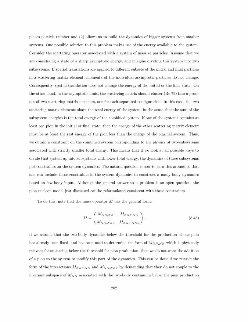
places particle number and (2) allows us to build the dynamics of bigger systems from smaller

systems. One possible solution to this problem makes use of the energy available to the system.

Consider the scattering operator associated with a system of massive particles. Assume that we

are considering a state of a sharp asymptotic energy, and imagine dividing this system into two

subsystems. If spatial translations are applied to different subsets of the initial and final particles

in a scattering matrix element, momenta of the individual asymptotic particles do not change.

Consequently, spatial translation does not change the energy of the initial or the final state. On

the other hand, in the asymptotic limit, the scattering matrix should cluster (Re 79) into a prod-

uct of two scattering matrix elements, one for each separated configuration. In this case, the two

scattering matrix elements share the total energy of the system, in the sense that the sum of the

subsystem energies is the total energy of the combined system. If one of the systems contains at

least one pion in the initial or final state, then the energy of the other scattering matrix element

must be at least the rest energy of the pion less than the energy of the original system. Thus,

we obtain a constraint on the combined system corresponding to the physics of two-subsystems

associated with strictly smaller total energy. This means that if we look at all possible ways to

divide that system up into subsystems with lower total energy, the dynamics of these subsystems

put constraints on the system dynamics. The natural question is how to turn this around so that

one can include these constraints in the system dynamics to construct a many-body dynamics

based on few-body input. Although the general answer to is problem is an open question, the

pion nucleon model just discussed can be reformulated consistent with these constraints.

To do this, note that the mass operator M has the general form:

M =

(MNN,NN MNNπ,NN

MNN,NNπ MNNπ,NNπ

). (8.48)

If we assume that the two-body dynamics below the threshold for the production of one pion

has already been fixed, and has been used to determine the form of MNN,NN which is physically

relevant for scattering below the threshold for pion production, then we do not want the addition

of a pion to the system to modify this part of the dynamics. This can be done if we restrict the

form of the interactions MNNπ,NN and MNN,NNπ by demanding that they do not couple to the

invariant subspace of MNN associated with the two-body continuum below the pion production

202

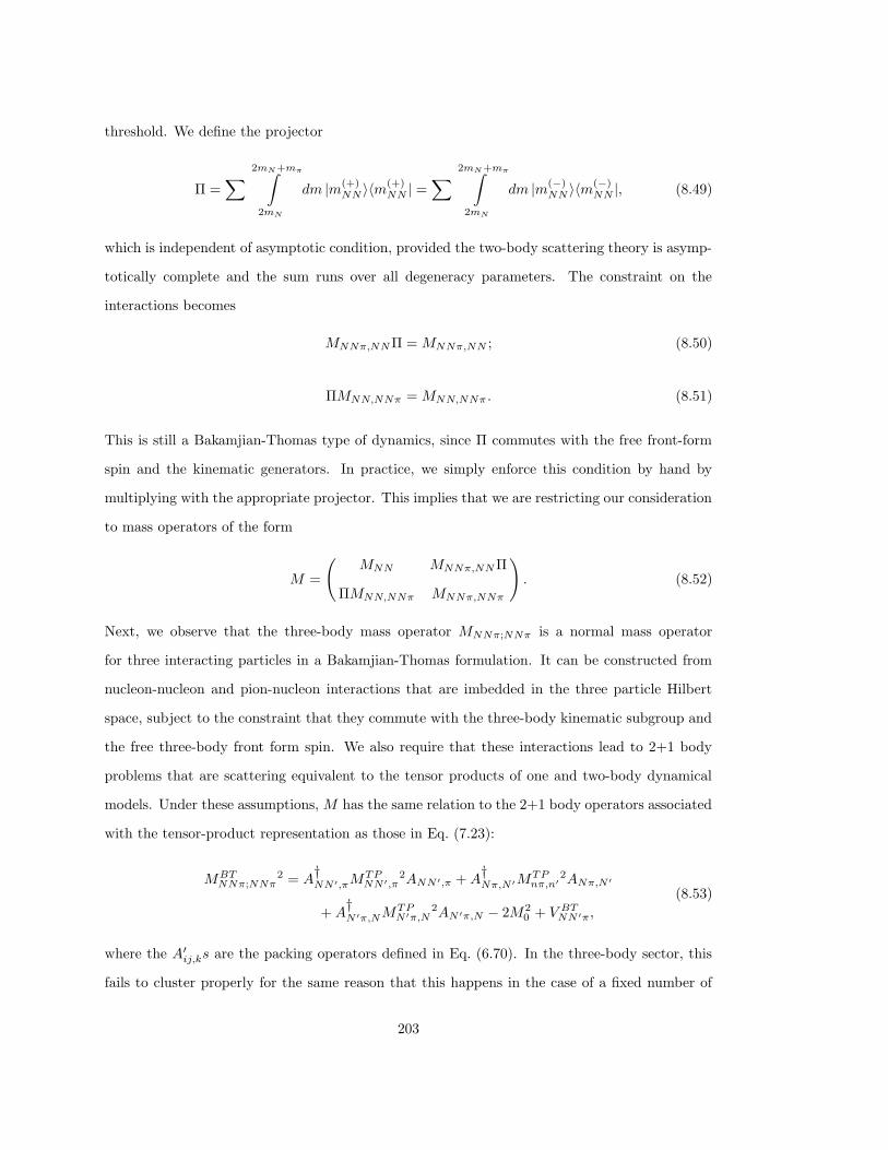
threshold. We define the projector

Π =∑ 2mN+mπ∫

2mN

dm |m(+)NN 〉〈m(+)

NN | =∑ 2mN+mπ∫

2mN

dm |m(−)NN 〉〈m(−)

NN |, (8.49)

which is independent of asymptotic condition, provided the two-body scattering theory is asymp-

totically complete and the sum runs over all degeneracy parameters. The constraint on the

interactions becomes

MNNπ,NNΠ = MNNπ,NN ; (8.50)

ΠMNN,NNπ = MNN,NNπ . (8.51)

This is still a Bakamjian-Thomas type of dynamics, since Π commutes with the free front-form

spin and the kinematic generators. In practice, we simply enforce this condition by hand by

multiplying with the appropriate projector. This implies that we are restricting our consideration

to mass operators of the form

M =

(MNN MNNπ,NNΠ

ΠMNN,NNπ MNNπ,NNπ

). (8.52)

Next, we observe that the three-body mass operator MNNπ;NNπ is a normal mass operator

for three interacting particles in a Bakamjian-Thomas formulation. It can be constructed from

nucleon-nucleon and pion-nucleon interactions that are imbedded in the three particle Hilbert

space, subject to the constraint that they commute with the three-body kinematic subgroup and

the free three-body front form spin. We also require that these interactions lead to 2+1 body

problems that are scattering equivalent to the tensor products of one and two-body dynamical

models. Under these assumptions, M has the same relation to the 2+1 body operators associated

with the tensor-product representation as those in Eq. (7.23):

MBTNNπ;NNπ

2 = A†NN ′,πM

TPNN ′,π

2ANN ′,π +A†Nπ,N ′M

TPnπ,n′

2ANπ,N ′

+A†N ′π,NM

TPN ′π,N

2AN ′π,N − 2M20 + V BT

NN ′π,

(8.53)

where the A′ij,ks are the packing operators defined in Eq. (6.70). In the three-body sector, this

fails to cluster properly for the same reason that this happens in the case of a fixed number of

203

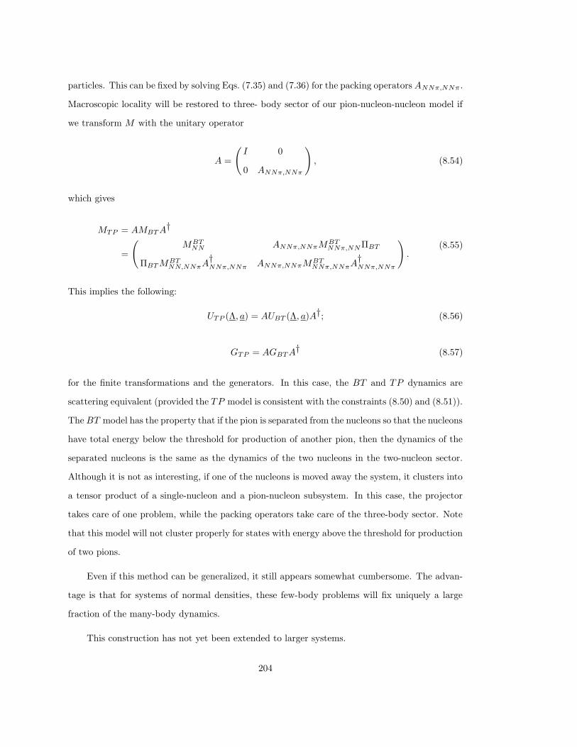
particles. This can be fixed by solving Eqs. (7.35) and (7.36) for the packing operators ANNπ,NNπ .

Macroscopic locality will be restored to three- body sector of our pion-nucleon-nucleon model if

we transform M with the unitary operator

A =

(I 0

0 ANNπ,NNπ

), (8.54)

which gives

MTP = AMBTA†

=

(MBT

NN ANNπ,NNπMBTNNπ,NNΠBT

ΠBTMBTNN,NNπA

†NNπ,NNπ ANNπ,NNπM

BTNNπ,NNπA

†NNπ,NNπ

).

(8.55)

This implies the following:

UTP (Λ, a) = AUBT (Λ, a)A†; (8.56)

GTP = AGBTA† (8.57)

for the finite transformations and the generators. In this case, the BT and TP dynamics are

scattering equivalent (provided the TP model is consistent with the constraints (8.50) and (8.51)).

TheBT model has the property that if the pion is separated from the nucleons so that the nucleons

have total energy below the threshold for production of another pion, then the dynamics of the

separated nucleons is the same as the dynamics of the two nucleons in the two-nucleon sector.

Although it is not as interesting, if one of the nucleons is moved away the system, it clusters into

a tensor product of a single-nucleon and a pion-nucleon subsystem. In this case, the projector

takes care of one problem, while the packing operators take care of the three-body sector. Note

that this model will not cluster properly for states with energy above the threshold for production

of two pions.

Even if this method can be generalized, it still appears somewhat cumbersome. The advan-

tage is that for systems of normal densities, these few-body problems will fix uniquely a large

fraction of the many-body dynamics.

This construction has not yet been extended to larger systems.

204

9. Electromagnetic Currents and Tensor Operators

An important application of relativistic quantum mechanical models is the calculation of

observables associated with the interaction of electrons, photons and other weak probes with

hadronic targets.

Such calculations focus on the evaluation of matrix elements of a hadronic current operator

Iµh (x) in applications of the one-photon-exchange approximation. In the first part of this section,

we provide expressions for observables in terms of matrix elements of the hadronic electromagnetic

current operator evaluated in eigenstates of the strong Hamiltonian. A complete measurement of

the cross section can be used to determine these matrix elements up to an overall phase. We also

exhibit the relation between these current matrix elements and observables in inclusive scattering,

where only the final electron is measured.

Poincare covariance, current conservation, and discrete symmetries imply relations between

different current matrix elements. Because of these constraints, all of the matrix elements can

be determined, using Poincare covariance, current conservation, and discrete symmetries, from a

maximal set of independent matrix elements. Alternatively, one can classify the matrix elements

in terms of a set of Lorentz invariant form factors, which contain the same information as the

maximal set of independent matrix elements. In the second part of this section, we present

a general classification scheme for matrix elements of tensor operators, which amounts to a

Wigner-Eckart theorem for the Poincare group. We also show the reduction to a maximal set of

independent matrix elements can be especially simple in the front form.

In general, the number of independent matrix elements is the same as the number of invariant

form factors. Form factors are a conveniently chosen maximal set of independent functions of the

independent matrix elements that also contain the same information as the form factors.

In the last part of this section, we discuss the actual computation of matrix elements of the

hadronic current operator. The conditions of current covariance and continuity put dynamical

constraints on the current operator. The problem is that the classical picture of a current being

constructed from charges and convection currents of each constituent is not consistent with ei-

ther current conservation or with relativity. The difficulty for theorists is that although current

205

conservation and relativity constrain the hadronic current operator, they do not fix this operator.

These issues are not limited to phenomenological models of hadrons; the same problem occurs

when the hadrons are described by local fields. In spite of these difficulties, it is possible to for-

mulate a sensible invariant impulse approximation using front-form dynamics. This is illustrated

for the case of the π → ρ transition form factor.

9.1. Basic Formulas and Observables

For electron scattering from strongly interacting systems, the complete Hamiltonian can be

written as follows:

H = HQED +Hh +Hem, (9.1)

where HQED is the Hamiltonian of photons and electrons, Hh the hadronic system, and Hem the

interaction between radiation and matter:

Hem = e

∫d3x Iµ(x)Aµ(x), (9.2)

where

Iµ = Iµh + Iµ

e , (9.3)

is the sum of the hadronic and electron current densities and we use units of electric charge

where α = e2/4π is the fine structure constant. We use a convention where the electron charge

is factored out of the current density operators. The current density must transform covariantly:

U(Λ, a)Iµ(x)U(Λ, a)† = (Λ−1)µνI

ν(Λx+ a), (9.4)

and it must be conserved with respect to the four-momentum:

gµν [Pµ, Iν(x)] = 0. (9.5)

The representation U(Λ, a) of P in Eq. (9.4) is associated with the interacting lepton-hadron

system. In what follows, we employ the one-photon-exchange approximation, or more generally,

206

we consider QED at tree level. In this case, the representation U(Λ, a), of P , in Eq. (9.4) can be

replaced by

U(Λ, a) → Uh(Λ, a) ⊗ UQED(Λ, a). (9.6)

In the one-photon-exchange approximation, the hadronic representation, Uh(Λ, a), has no ra-

diative corrections (these go beyond the one-photon-exchange contribution), and the constraints

(9.4) and (9.5) become

Uh(Λ, a)Iµh (x)Uh(Λ, a)† = (Λ−1)µ

νIνh(Λx+ a), (9.7)

and

gµν [Pµh , I

νh(x)] = 0. (9.8)

For the treatment of electron scattering from large-Z nuclei, where one-photon exchange is not

appropriate, the radiative corrections to Uh(Λ, a) must be considered. Such problems are not

considered here.

The scattering cross section in the one-photon-exchange approximation can be determined

using time ordered perturbation theory in the interaction representation. For a single-particle

initial state, the calculation is summarized by the equations

dσ =(2π)4

|sv| |〈k′η′;p′1µ

′1; · · · ;p′Nµ′N (+)‖T‖kη;pµ〉|2dΦN ; (9.9)

〈f |S|i〉 = 1 − (2π)iδ4(p′ − p)〈f‖T‖i〉, (9.10)

S = T exp(−i∫dtHem)

≈ I − i

∫d4xHem(x) +

(−i)22!

∫d4x1

∫d4x2 T (Hem(x1),Hem(x2)),

(9.11)

where k and k′ are the initial and final electron momenta, p and p′j are the initial and final

hadron momenta, and T denotes time ordering. The phase space factor is

dΦN =

N∏

i=1

d3p′id3k′δ4(

N∑

j=1

p′j + k′ − p− k), (9.12)

where s is a statistical factor equal to the number of permutations of identical particles in the

final state, and the relative speed of the electron and target can be expressed in the form (Mo 45,

207

Br 59):

1

|v| =ωme

(k)ωm(p)√(p · k)2 −m2

em2. (9.13)

The (+) superscript on the final hadron state indicates that this is an eigenstate of the hadronic

Hamiltonian that asymptotically approaches a plane-wave state as t → +∞, where the plane-

wave states have a delta function normalization:

〈p′µ′|pµ〉 = δµ′µδ(p′ − p). (9.14)

The initial state is also an eigenstate of the hadronic Hamiltonian, but the target is usually bound

(or elementary), and thus does not require a scattering asymptotic condition.

Spacetime translational invariance of the electron and hadron current matrix elements can be

used to express the one-photon exchange contribution to the reduced matrix element 〈f‖T fi‖i〉

in the form:

〈k′ η′ p′1 µ′1 ; · · · ; p′N µ′N(+)‖T‖k η pµ〉

= −ie2(2π)3∫d4xe−i(k′−k)·x〈0|T [Aµ(0)Aν(x)]|0〉

× 〈k′ η′|Iµe (0)|k η〉〈p′1 µ′1 · · · ;p′N µ′N

(+)|Iνh(0)|pµ〉.

(9.15)

The photon propagator is

gµν

−q2 + i0+= −i

∫d4x eiq·x〈0|T [Aµ(0)Aν(x)]|0〉, (9.16)

where

q = k − k′ = p′ − p (9.17)

is the momentum transferred to the target. This gives the following expression for the reduced

matrix element:

〈k′ η′ p′1 µ′1 ; · · · ;p′N µ′N(+)‖T‖k η pµ〉

= e2(2π)3gµν

−q2 + i0+〈k′ η′|Iµ

e (0)|k η〉〈p′1 µ′1 ; · · · ;p′N µ′N(+)|Iν

h(0)|pµ〉.(9.18)

The electron current matrix elements can be expressed in terms of a free electron field Ψ:

〈k′ η′|Iµe (0)|k η〉 = e〈0|a(k′, η′) : Ψ(0)γµΨ(0) : a†(k, η)|0〉. (9.19)

The electron field satisfies canonical equal time anticommutation relations, and the electron

208

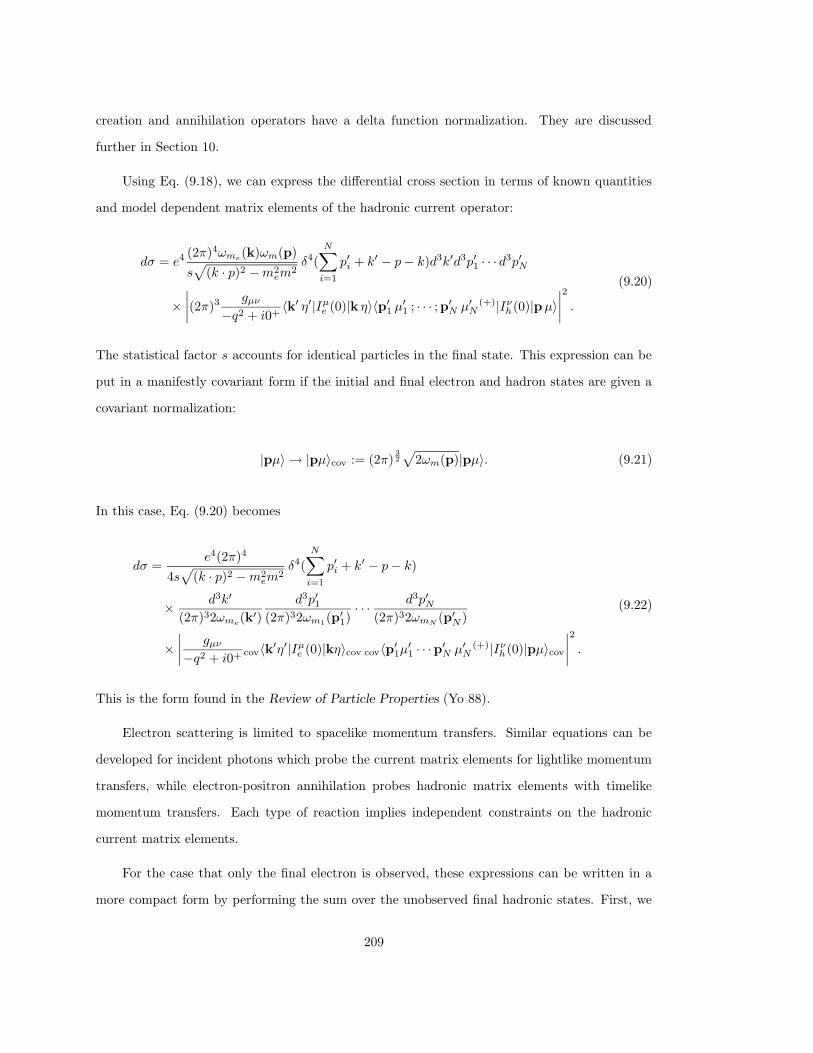
creation and annihilation operators have a delta function normalization. They are discussed

further in Section 10.

Using Eq. (9.18), we can express the differential cross section in terms of known quantities

and model dependent matrix elements of the hadronic current operator:

dσ = e4(2π)4ωme

(k)ωm(p)

s√

(k · p)2 −m2em

2δ4(

N∑

i=1

p′i + k′ − p− k)d3k′d3p′1 · · · d3p′N

×∣∣∣∣(2π)3

gµν

−q2 + i0+〈k′ η′|Iµ

e (0)|k η〉〈p′1 µ′1 ; · · · ;p′N µ′N(+)|Iν

h(0)|pµ〉∣∣∣∣2

.

(9.20)

The statistical factor s accounts for identical particles in the final state. This expression can be

put in a manifestly covariant form if the initial and final electron and hadron states are given a

covariant normalization:

|pµ〉 → |pµ〉cov := (2π)32

√2ωm(p)|pµ〉. (9.21)

In this case, Eq. (9.20) becomes

dσ =e4(2π)4

4s√

(k · p)2 −m2em

2δ4(

N∑

i=1

p′i + k′ − p− k)

× d3k′

(2π)32ωme(k′)

d3p′1(2π)32ωm1

(p′1)· · · d3p′N

(2π)32ωmN(p′N )

×∣∣∣∣

gµν

−q2 + i0+ cov〈k′η′|Iµe (0)|kη〉cov cov〈p′1µ′1 · · ·p′N µ′N

(+)|Iνh(0)|pµ〉cov

∣∣∣∣2

.

(9.22)

This is the form found in the Review of Particle Properties (Yo 88).

Electron scattering is limited to spacelike momentum transfers. Similar equations can be

developed for incident photons which probe the current matrix elements for lightlike momentum

transfers, while electron-positron annihilation probes hadronic matrix elements with timelike

momentum transfers. Each type of reaction implies independent constraints on the hadronic

current matrix elements.

For the case that only the final electron is observed, these expressions can be written in a

more compact form by performing the sum over the unobserved final hadronic states. First, we

209

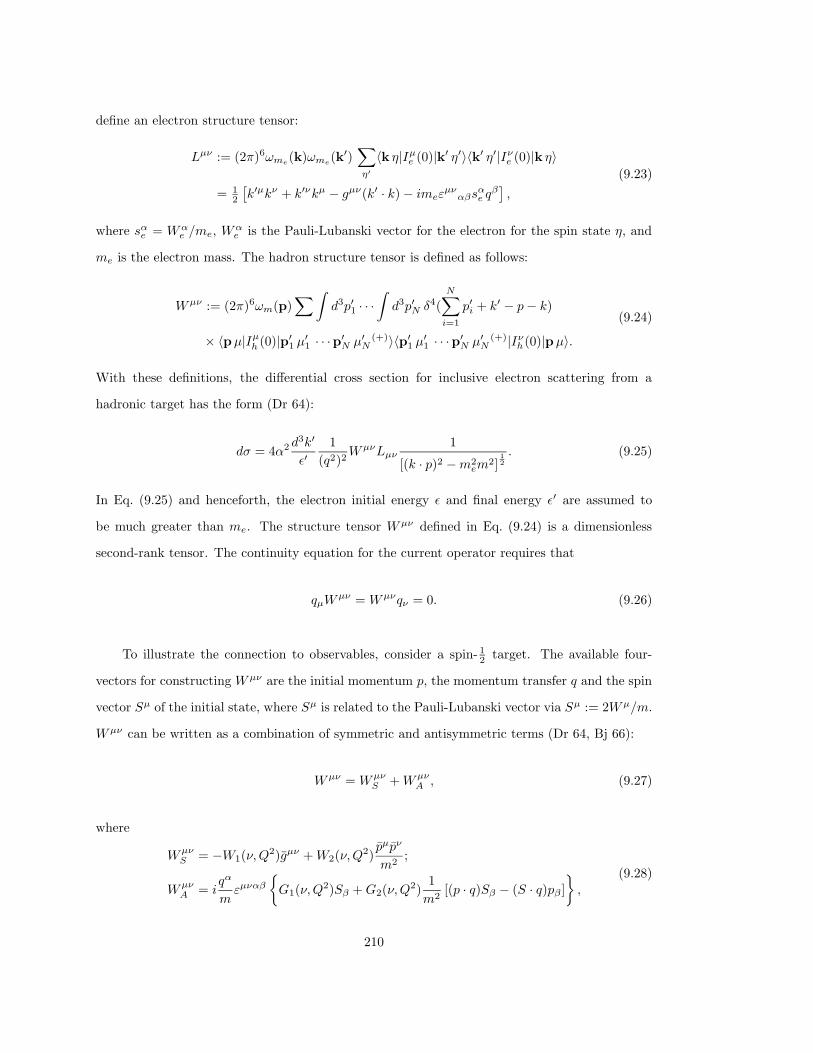
define an electron structure tensor:

Lµν := (2π)6ωme(k)ωme

(k′)∑

η′

〈k η|Iµe (0)|k′ η′〉〈k′ η′|Iν

e (0)|k η〉

= 12

[k′µkν + k′νkµ − gµν(k′ · k) − imeε

µναβs

αe q

β],

(9.23)

where sαe = Wα

e /me, Wαe is the Pauli-Lubanski vector for the electron for the spin state η, and

me is the electron mass. The hadron structure tensor is defined as follows:

Wµν := (2π)6ωm(p)∑∫

d3p′1 · · ·∫d3p′N δ4(

N∑

i=1

p′i + k′ − p− k)

× 〈pµ|Iµh (0)|p′1 µ′1 · · ·p′N µ′N

(+)〉〈p′1 µ′1 · · ·p′N µ′N(+)|Iν

h(0)|pµ〉.(9.24)

With these definitions, the differential cross section for inclusive electron scattering from a

hadronic target has the form (Dr 64):

dσ = 4α2 d3k′

ε′1

(q2)2WµνLµν

1

[(k · p)2 −m2em

2]12

. (9.25)

In Eq. (9.25) and henceforth, the electron initial energy ε and final energy ε′ are assumed to

be much greater than me. The structure tensor W µν defined in Eq. (9.24) is a dimensionless

second-rank tensor. The continuity equation for the current operator requires that

qµWµν = Wµνqν = 0. (9.26)

To illustrate the connection to observables, consider a spin- 12 target. The available four-

vectors for constructing W µν are the initial momentum p, the momentum transfer q and the spin

vector Sµ of the initial state, where Sµ is related to the Pauli-Lubanski vector via Sµ := 2Wµ/m.

Wµν can be written as a combination of symmetric and antisymmetric terms (Dr 64, Bj 66):

Wµν = WµνS +Wµν

A , (9.27)

where

WµνS = −W1(ν,Q

2)gµν +W2(ν,Q2)pµpν

m2;

WµνA = i

qα

mεµναβ

G1(ν,Q

2)Sβ +G2(ν,Q2)

1

m2[(p · q)Sβ − (S · q)pβ ]

,

(9.28)

210

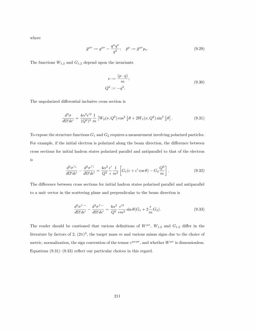
where

gµν := gµν − qµqν

q2; pµ := gµνpν . (9.29)

The functions W1,2 and G1,2 depend upon the invariants

ν :=(p · q)m

;

Q2 := −q2.(9.30)

The unpolarized differential inclusive cross section is

d2σ

dΩ′dε′=

4α2ε′2

(Q2)21

m

[W2(ν,Q

2) cos2 12θ + 2W1(ν,Q

2) sin2 12θ]. (9.31)

To expose the structure functionsG1 andG2 requires a measurement involving polarized particles.

For example, if the initial electron is polarized along the beam direction, the difference between

cross sections for initial hadron states polarized parallel and antiparallel to that of the electron

is

d2σ↑↓

dΩ′dε′− d2σ↑↑

dΩ′dε′=

4α2

Q2

ε′

ε

1

m2

[G1(ε+ ε′ cos θ) −G2

Q2

m

]. (9.32)

The difference between cross sections for initial hadron states polarized parallel and antiparallel

to a unit vector in the scattering plane and perpendicular to the beam direction is

d2σ↑→

dΩ′dε′− d2σ↑←

dΩ′dε′=

4α2

Q2

ε′2

εm2sin θ(G1 + 2

ε

mG2). (9.33)

The reader should be cautioned that various definitions of W µν , W1,2 and G1,2 differ in the

literature by factors of 2, (2π)3, the target mass m and various minus signs due to the choice of

metric, normalization, the sign convention of the tensor εµνρσ, and whether Wµν is dimensionless.

Equations (9.31)–(9.33) reflect our particular choices in this regard.

211

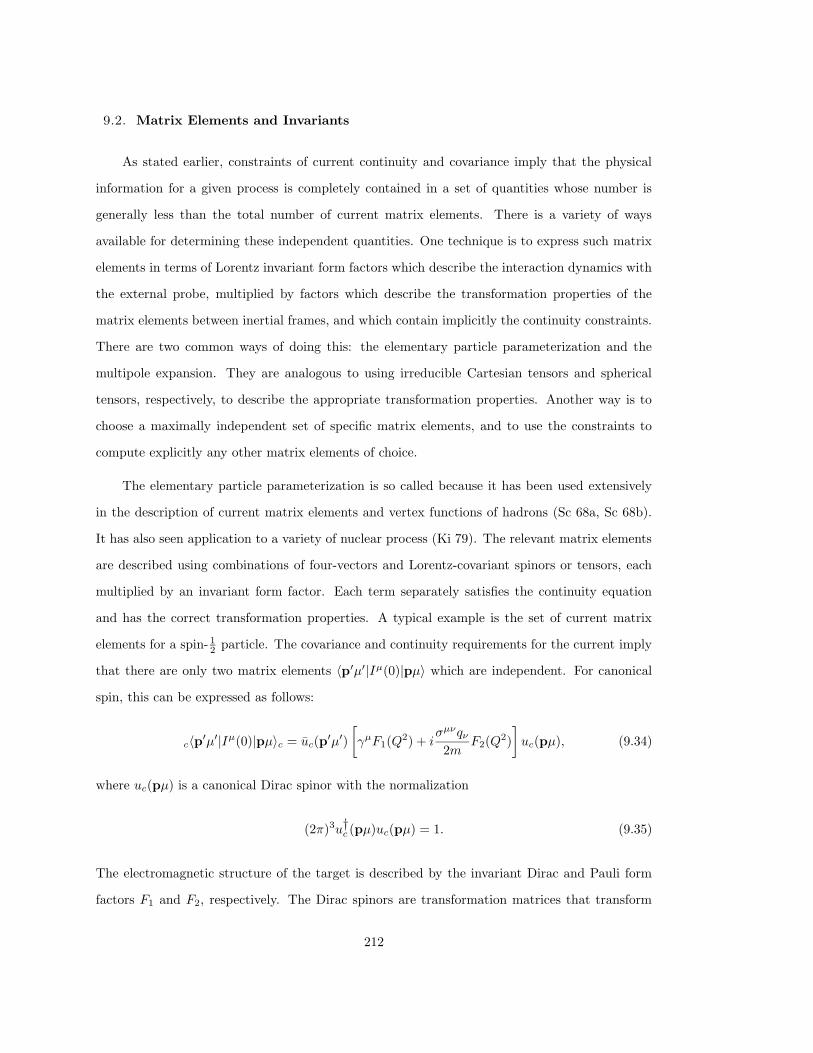
9.2. Matrix Elements and Invariants

As stated earlier, constraints of current continuity and covariance imply that the physical

information for a given process is completely contained in a set of quantities whose number is

generally less than the total number of current matrix elements. There is a variety of ways

available for determining these independent quantities. One technique is to express such matrix

elements in terms of Lorentz invariant form factors which describe the interaction dynamics with

the external probe, multiplied by factors which describe the transformation properties of the

matrix elements between inertial frames, and which contain implicitly the continuity constraints.

There are two common ways of doing this: the elementary particle parameterization and the

multipole expansion. They are analogous to using irreducible Cartesian tensors and spherical

tensors, respectively, to describe the appropriate transformation properties. Another way is to

choose a maximally independent set of specific matrix elements, and to use the constraints to

compute explicitly any other matrix elements of choice.

The elementary particle parameterization is so called because it has been used extensively

in the description of current matrix elements and vertex functions of hadrons (Sc 68a, Sc 68b).

It has also seen application to a variety of nuclear process (Ki 79). The relevant matrix elements

are described using combinations of four-vectors and Lorentz-covariant spinors or tensors, each

multiplied by an invariant form factor. Each term separately satisfies the continuity equation

and has the correct transformation properties. A typical example is the set of current matrix

elements for a spin- 12 particle. The covariance and continuity requirements for the current imply

that there are only two matrix elements 〈p′µ′|Iµ(0)|pµ〉 which are independent. For canonical

spin, this can be expressed as follows:

c〈p′µ′|Iµ(0)|pµ〉c = uc(p′µ′)

[γµF1(Q

2) + iσµνqν2m

F2(Q2)

]uc(pµ), (9.34)

where uc(pµ) is a canonical Dirac spinor with the normalization

(2π)3u†c (pµ)uc(pµ) = 1. (9.35)

The electromagnetic structure of the target is described by the invariant Dirac and Pauli form

factors F1 and F2, respectively. The Dirac spinors are transformation matrices that transform

212

Wigner rotations to finite dimensional representations of SL(2, C). Equation (9.34) applies

equally well to the ground state of a 3H nucleus. For each value of Q2, it is sufficient to calculate

two independent matrix elements to fix the form factors F1(Q2) and F2(Q

2). Given the form

factors, Eq. (9.34) can be used to determine all remaining matrix elements corresponding to the

same Q2.

The multipole expansion has frequently been applied in nuclear physics, both for photon

transitions (Bl 52), and for the study of inelastic electroexcitation of discrete states of the nucleus

(De 66). The corresponding parameterization of the nucleon current matrix element employs the

Sachs form factors. In the Breit frame of the nucleon,

p = − 12q; p′ = 1

2q, (9.36)

the matrix elements for canonical spin are

c〈 12qµ

′|I0(0)| − 12qµ〉c =

GE(Q2)

1 + τδµ′µ; τ :=

Q2

4m2;

c〈 12qµ

′|I(0)| − 12qµ〉c =

GM(Q2)

1 + τ

1

2m[iσ × q]µ′µ .

(9.37)

In the multipole expansion, matrix elements are expanded in terms of rotational invariants in a

particular frame, and are related to matrix elements in other frame by the appropriate explicit

transformation coefficients. While this approach is not manifestly Lorentz covariant, it is com-

pletely equivalent to the elementary particle approach, containing the same amount of physical

information and having the correct transformation properties. In practice, the form factors can

be determined by calculating two independent matrix elements.

Since the elementary particle approach is manifestly covariant and is discussed extensively

elsewhere, we have chosen to examine the multipole expansion in this section.

Matrix Elements of Tensor Operators In this section, we discuss ways to represent matrix

elements of Lorentz tensor operators, such as field operators or current operators, as products of

transformation coefficients (which guarantee the covariance) with invariant form factors (which

define the operator).

213

In quantum field theories, Hermitian operators corresponding to quantum mechanical ob-

servables are built out of local fields that transform covariantly under the Lorentz group. In the

same way that any finite dimensional unitary representation of the rotation group can be built up

out of spin- 12 representations, it is possible to build operators that transform irreducibly under

any finite dimensional representation of the Lorentz group in terms of basic building blocks. The

result is that any Lorentz covariant field can be constructed out of these irreducible parts.

There are two differences between the Lorentz group and the rotation group. The first is

that the finite dimensional representations of the Lorentz group are built out of representations

of SL(2, C) rather than SU(2). The second is that there are two inequivalent representations of

SL(2, C) that play the role analogous to that of SU(2) in the case of rotations. Up to a similarity

transformation, these representations are given in terms of the SL(2, C) matrices Λ and their

inverse adjoints (Λ−1)†. These matrices are not the same because they are not unitary, and there

is no similarity transformation which relates them.

We introduce the following convention (St 64, Be 82) for SL(2, C) spinors: an upper (undot-

ted) spinor index transforms by right multiplication by Λ, a lower dotted index, i.e., β transforms

by right multiplication with (Λ−1)†, a lower undotted spinor index transforms by right multipli-

cation with (Λ−1)T , where T denotes transpose, and an upper dotted index transforms by right

multiplication by Λ∗. The ‘metric spinor’

ε := iσ2. (9.38)

is the similarity transformation relating the two dotted or two undotted representations:

εΛε−1 = (Λ−1)T ; εΛ∗ε−1 = (Λ−1)† (9.39)

Right multiplication by ε lowers an index, and right multiplication by ε−1 raises an index.

We are now in a position to define the basic building blocks from which one builds all

Lorentz covariant fields that transform according to finite dimensional representations of the

Lorentz group. An irreducible spinor field operator of rank (m,n) is an operator valued function

214

of the spacetime coordinates with rank (m,n) spinor indices:

Ψα1···αm

β1···βn

(x). (9.40)

It is symmetric in the m undotted and n dotted indices respectively, and transforms under the

Poincare group as follows:

U(Λ, a)Ψα1···αm

β1···βn(x)U†(Λ, a)

= Ψζ1···ζm

η1···ηn(Λx+ a)Λζ1α1

· · ·Λζmαm(Λ−1)

†η1β1

· · · (Λ−1)†ηnβn

.(9.41)

Indices on Ψ can be raised and lowered using ε. Upper and lower dotted index or upper and

lower undotted index can be contracted with the result transforming like a pseudoscalar.

We can use these irreducible representations to construct any type of Lorentz covariant

field. As will be shown below, four-vectors transform as a rank (1,1) spinors. The rank (0, 0)

representation corresponds to a scalar field. A Dirac spinor transforms like a (1, 0) ⊕ (0, 1)

representation. The rank (1, 0) and (0, 1) spinors correspond to right- and left-handed spin-

12 fields. The rank (2, 0) and (0, 2) representations correspond to antisymmetric second rank

tensors that are self-dual and anti-self-dual, respectively (Ra 81). The Maxwell field strength

tensor Fµν transforms as a direct sum (2, 0) ⊕ (0, 2) representation.

Space reflection and time reversal can be expressed as follows:

PΨα1···αm

β1···βn(x)P−1 = Ψ∗β1···βn

α1···αm(Px) (9.42)

and

TΨα1···αm

β1···βn

(x)T−1 = (i)m+nΨ∗β1···βn

α1···αm(Tx). (9.43)

Note also that for the special case where Λ is a rotation R,

R = (R†)−1. (9.44)

This property is very useful in the discussion below.

215

Before we discuss matrix elements of tensor fields, it is useful to compare the transformation

properties of these fields with particle states. In the case of the fields, the discrete indices

transform under representations of the Lorentz group, while in the particle case they transform

under a representation of a subgroup that leaves a given four-momentum invariant. For spacelike

four-momentum, this subgroup is the rotation group and the resulting transformations are Wigner

rotations. The transformations of the discrete indices of the particles and fields are not really

different. They are equivalent ways of representing the same transformation. This point is not

generally appreciated and often causes confusion regarding the need for four-component spinors to

treat spin- 12 particles. To understand the relation between Lorentz spinors and Poincare spinors,

let Ψαβ(p) be the Fourier transform of a rank (1, 1) spinor field. Clearly, the spinor indices in the

Fourier transformed field transform like the indices in Eq. (9.41). Let us assume for the moment

that p is timelike, and consider the transformation properties of the linear combination with p

dependent coefficients:

Ψζη(p)Lc(p)ζαL

−1c

†(p)ηβ . (9.45)

A direct calculation shows that all of the Lorentz transformations of the discrete indices are

replaced Wigner rotations. What is more important is that rotations of dotted and undotted

indices are the same. In this case, the transformed dotted and undotted indices are no longer

inequivalent and can be related by linear transformations; there is no need for four-component

objects to describe a spin 12 system if done using irreducible representation of the Poincare group.

It is legitimate to ask: why use Lorentz covariant spinor densities to make fields rather than

irreducible Poincare covariant tensor operators? The reason is that when p changes from spacelike

to lightlike to timelike, the indices of irreducible Poincare covariant operators transform under

different “little groups” for each case (Mo 65). If these “little groups” are used explicitly, they

obscure the analytic properties of the field, which are important in the proof of general properties

of field operators. Irreducible representations of the Poincare group are used to describe particles,

however, because in that case the four-momentum is timelike (for particles with m 6= 0), and

the representations are unitary. Note that the equivalence between these representations requires

that the field operator has a spacetime argument in addition to the discrete indices. Nothing is

lost in using Eq. (9.45) because the transformations therein are invertible.

216

The quantities of interest are matrix elements of an irreducible Lorentz tensor field evaluated

between physical particle states. The particle states will be assumed to transform irreducibly

under the action of the Poincare group. To treat multiparticle final states the Clebsch-Gordan

coefficients of the Poincare group can be used to express the desired final states as a linear

combination of states that transform irreducibly. Examples of these quantities are current matrix

elements, Bethe-Salpeter amplitudes, Blankenbecler-Cook amplitudes (Bl 60), and N -quantum

amplitudes (Gr 65a).

We are interested in matrix elements of tensor operators of the form

〈m′j′;p′µ′|Ψα1···αm

β1···βn(0)|mj;pµ〉.

As a first step, we consider matrix elements

〈m′j′;p′µ′|Ψαβ(0)|mj;pµ〉,

containing one index each of the two inequivalent representations of SL(2, C). While there are

2 × 2 × (2j + 1) × (2j ′ + 1) separate matrix elements for each fixed p and p′, they are not all

independent. The covariance properties of the operator provide constraints which relate various

matrix elements to each other. There may be other constraint such as parity, time reversal and

current continuity that further reduce the number of independent matrix elements. For now, we

focus on the covariance requirements.

As a preliminary exercise for studying matrix elements of current operators, we consider the

operator Ψαβ(x) – more specifically, Ψα

β(0), and the set of matrix elements c〈m′j′;p′µ′|Ψα

β(0)|mj;pµ〉c.

It is useful to consider the Fourier transform:

Ψαβ(q) :=

1

(2π)4

∫d4x e−iq·xΨα

β(x). (9.46)

By translational invariance, we get

c〈m′j′;p′µ′|Ψαβ(q)|mj;pµ〉c

=1

(2π)4

∫d4x e−iq·x

c〈m′j′;p′µ′|eip′·xΨαβ(0)e−ip·x|mj;pµ〉c

= δ4(p′ − p− q) c〈m′j′;p′µ′|Ψαβ(0)|mj;pµ〉c.

(9.47)

We are interested in kinematics where p′ := p + q is timelike, corresponding to a massive

217

final state. This means that there exists a frame where p′0 = (m′, 0). Let p0 + q0 = p′0 be

related to p and q with the same Lorentz transformation that relates p′0 to p′. Consider the state

vector∫dp0 Y

lµl

(p0)Ψαβ(q0)|mj;p0µ〉c. Under a rotation R, this linear combination transforms

as follows:

U(R)

∫dp0 Y

lµl

(p0)Ψαβ(q0)|mj;p0µ〉c

=∑∫

dp0 Ylµl

(p0)Ψζη(Rq0)|mj;Rp0µ〉cRζαRηβD

jµµ(R)

=∑∫

dp0 Ylµl

(p0)Ψζη(q0)|mj;p0µ〉cRζαRηβD

lµlµl

(R)Djµµ(R).

(9.48)

In Eq. (9.48), we have made use of the fact that (R†)−1 = R, that is, dotted and undotted

indices transform in the same way under rotations. Since all three indices transform with the

same argument R, they can be combined to construct the following state:

|[ΨlsJ ]m′j′; 0µ′〉c := 〈 12α

12 β|sµs〉〈lµlsµs|J µJ 〉〈jµJµJ |j′µ′〉

×∫dp0 Y

lµl

(p0)Ψαβ(q0)|mj;p0µ〉c,

(9.49)

where repeated indices are summed, and m′2 = −p′2. This linear combination can be boosted to

define a new state,

|[ΨlsJ ]m′j′;p′µ′〉c := 〈 12α

12 β|sµs〉〈lµlsµs|J µJ 〉〈jµJµJ |j′µ′j〉

×√

m′

ωm′(p′)U [Lc(p

′)]∫dp0 Y

lµl

(p0)Ψαβ(q0)|mj;p0µ〉c,

(9.50)

in the same manner as that of a particle of mass m′ and spin j′. The extra square root factor

gives this state the same transformation properties as a non-covariant normalized state vector.

From the above definitions and the transformation properties of the states, the inner product

of this newly defined state vector with the final state |m′′j′′;p′′µ′′〉c must have the form

c〈m′′j′′;p′′µ′′|[ΨlsJ ]m′j′;p′µ′〉c = δj′′j′δµ′′µ′δ(m′′ −m′)δ3(p′′ − p′)

× 〈m′′j′′‖ΨlsJ (q2)‖m′j′〉.(9.51)

The reduced matrix element 〈m′j′‖ΨlsJ (q2)‖mj〉 is Poincare invariant. We now make use of

Eq. (9.51) and invert the definition (9.50) to obtain the desired matrix elements c〈m′j′;p′µ′|Ψαβ(q)|mj;pµ〉c.

218

Under Lorentz transformations,

U(Λ)Ψαβ(q)U†(Λ) =

∑Ψζ

η(Λq)Λζα(Λ−1)†ηβ

; (9.52)

U(Λ)|mj;pµ〉c =

√ωm(Λp)

ωm(p)

∑|mj; Λpµ〉cDj

µµ[Rc(Λ, p)]. (9.53)

From Eq. (9.52), (9.53) and the orthogonality and completeness properties of spherical harmonics,

rotation matrices and rotational Clebsch-Gordan coefficients, we find


= δ(m′′ −m′)δ3(p′′ − p′)

√ωm′(p′)m′

√ωm(p0)

ωm(p)

×∑

〈 12ζ

12 η|sµs〉〈lµlsµs|J µJ 〉〈jµJ µJ |j′µ′j〉

× Y lµl

∗(p0)[L−1c (p′)]ζα[Lc(p

′)]†ηβD

j†µµ[Rc(Lc(p

′), p0)]〈m′j′‖ΨlsJ (q2)‖mj〉,

(9.54)

where

p0 := L−1c (p′)p. (9.55)

Since

δ(m′′ −m′) =m′

p′0δ(p′′0 − p′0), (9.56)

we have


=

√m′

ωm′(p′)

√ωm(p0)

ωm(p)δ4(p′′ − p′)

∑〈 12ζ

12 η|sµs〉〈lµlsµs|J µJ 〉〈jµJ µJ |j′µ′〉

× Y lµl

∗(p0)[L−1c (p′)]ζα[Lc(p

′)]†ηβD

j†µµ[Rc(Lc(p

′), p)]〈m′j′‖ΨlsJ (q2)‖mj〉.

(9.57)

Matrix elements of Ψαβ(0) can be obtained via Eq. (9.45):

c〈m′j′;p′µ′|Ψαβ(0)|mj;pµ〉c

=

√m′

ωm′(p′)

√ωm(p0)

ωm(p)

∑〈 12ζ


× Y lµl

∗(p0)[L−1c (p′)]ζα[Lc(p

′)]†ηβD

j†µµ[Rc(Lc(p

′), p0)]〈m′j′‖ΨlsJ (q2)‖mj〉.

(9.58)

219

In a frame where the final state is at rest, Eq. (9.58) has an even simpler form:

c〈m′j′;0µ′|Ψαβ(0)|mj;p0µ〉c =

∑〈 12α

12 β|sµs〉〈lµlsµs|J µJ 〉〈jµJµJ |j′µ′〉

× Y lµl

∗(p0)〈m′j′‖ΨlsJ (q2)‖mj〉.(9.59)

Although Eq. (9.58) does not appear covariant because of the appearance of explicit indices, it

does in fact have the correct transformation properties. Put another way, what we have done

is to obtain matrix elements of Ψαβ(0) in an arbitrary frame by relating them to corresponding

matrix elements in the final state rest frame.

Equation (9.58) also has the appearance of a nonrelativistic Wigner-Eckart theorem for tensor

operators of this type, but with extra kinematic factors and Wigner rotations which disappear

in the nonrelativistic limit. Note also that these expressions summarize the symmetry associated

with Poincare invariance, but not the additional constraints associated with parity, time reversal

or current conservation which may further decrease the number of independent reduced matrix

elements. Parity and time reversal constraint can be determined by using Eq. (9.42)- (9.43) with

(9.58). We now sketch the necessary steps for constructing invariants associated with matrix

elements of the general type:

〈m′j′;p′µ′|Ψα1···αm

β1···βn(0)|mj;pµ〉.

Consider the state vector∫dp0 Y

lµl

(p0)Ψα1···αm

β1···βn(q0)|mj;p0µ〉c. Under a rotation R, this trans-

forms as follows:

U(R)

∫dp0 Y

lµl

(p0)Ψα1···αm

β1···βn(q0)|mj;p0µ〉c

=∑∫

dp0 Ylµl

(p0)Ψζ1···ζm

η1···ηn(q0)|mj;p0µ〉c

×Rζ1α1· · ·Rζmαm

Rη1β1· · ·Rηnβn

Dlµlµl

(R)Djµµ(R).

(9.60)

Since all indices transform with the same argument R, they can be combined using rotational

Clebsch-Gordan coefficients to form a state with indices J µJ . This then couples to the final state

just like a particle with the same mass and spin assignments. The order of coupling is a matter

of taste. The development then proceeds exactly as before, with the result similar to Eq. (9.58),

except for the presence of extra rotational Clebsch-Gordan coefficients, factors of L−1c (p), L†c (p)

and Wigner rotations.

220

Front-Form Matrix Elements Matrix elements of tensor operators between front-form state

vectors can be constructed directly from those given above in terms of canonical spin. The main

difference is that the index µ in a state vector |mj; pµ〉f does not transform the same way in

Eq. (9.48) as the corresponding index in a canonical-spin state vector. Under arbitrary rotations,

|mj; pµ〉f experiences a Wigner rotation which is not necessary the same as the rotation itself. In

order to make use of the development above for canonical spin, the front-form spins in Eq. (9.48)

must first undergo a Melosh rotation before being coupled together. The result is

f 〈m′j′; p′µ′|Ψαβ(0)|mj; pµ〉f

=

√m′

p′+

√p+0

p+

∑〈 12ζ


× Y lµl

∗(p0)[L−1f (p′)]ζα[Lf (p′)]†

ηβD

j†µµ[Rcf (p0)]〈m′j′‖ΨlsJ (q2)‖mj〉,

(9.61)

where

p0 := L−1f (p′)p, (9.62)

in contrast to Eq. (9.55) for canonical-spin matrix elements. Also, the front-form spins do not

undergo Wigner rotations for front-form boosts.

Example: Matrix Elements of Field Operators To illustrate the relations derived above,

we consider the matrix element

c〈m 12 ;pµp|ψ(0)|Md1;Pdµd〉c,

where |m 12 ;pµp〉c and |Md1;Pdµd〉c are state vectors for a nucleon and a deuteron, respectively,

and ψ(x) is a four-component nucleon field operator. It is more instructive to examine the matrix

element

c〈Md1;Pdµd|ψ†(0)|m 12 ;pµp〉c

in a frame where Pd = 0. As mentioned above, a Dirac field transforms like a (1, 0) ⊕ (0, 1)

representation, that is, a direct sum of a dotted and undotted spin- 12 spinors. In place of the dot-

ted and undotted spinors, we can use linear combinations ψe(x) and ψo(x), which have intrinsic

221

even and odd parity, respectively. They correspond to the usual u and v spinors (Bj 64) for free

fermions. The field operator ψ(x) can then be expressed as follows:

ψ(x) =∑

µs=± 12

[ψe

µs(x) + ψo

µs(x)]. (9.63)

Although the dotted and undotted spinors transform differently under boosts, we only make use

of the fact that they transform in the same way under rotations when Pd = 0. From Eq. (9.59),

we obtain

c〈Md1; 0µd|ψ†(0)|m 12 ;p0µp〉c

=∑

µs=± 12

〈lµl12µs|J µJ 〉〈 1

2µpJ µJ |1µd〉Y lµl

∗(p0)

×[〈Md1‖ψe

l12J

†(q2)‖m 12 〉 + 〈Md1‖ψo

l12J

†(q2)‖m 12 〉].

(9.64)

In place of the coupling scheme [ 12 ⊗ (l ⊗ 12 )J ]1, it is instructive to use the coupling scheme

[l ⊗ ( 12 ⊗ 1

2 )S]1, with the result:

c〈Md1; 0µd|ψ†(0)|m 12 ;p0µp〉c

=∑

µs=± 12

〈 12µp

12µs|SµS〉〈lµlSµS|1µd〉Y l

µl

∗(p0)

×[〈Md1‖ψe

l12S

†(q2)‖m 12 〉 + 〈Md1‖ψo

l12S

†(q2)‖m 12 〉].

(9.65)

where the reduced matrix elements in Eq. (9.65) are related to those in Eq. (9.64) by a 6j

coefficient. The parity of the spherical harmonic, together with the intrinsic parity of the field

operators, imply that l must be even for ψe and odd for ψo. The allowed couplings are therefore

3S1 and 3D1 for ψe and 3P1 and 1P1 for ψo. The last two arise from the explicit use of a

four-component field operator, and have been discussed extensively by Gross (Gr 65b).

Four-Vector Current Matrix Elements The current four-vector can be expressed as a ten-

sor operator which transforms as a product of inequivalent spin- 12 operators.

222

A 2×2 matrix I(x) can be defined in terms of the current operator Iµ(x) via

Iαβ(x) := [Iµ(x)σµ]αβ . (9.66)

which has the transformation property

U(Λ)I(x)U†(Λ) = Λ−1I(Λx)(Λ−1)†. (9.67)

It is more convenient to work with the matrix Iαβ(x) := [εI(x)]α

β(x). Under a Lorentz transfor-

mation,

U(Λ)Iαβ(x)U†(Λ) =

∑Iζη (Λx)Λζα(Λ−1)

†ηβ

(9.68)

That is, Iαβ(x) is a realization of the example developed above, with

Ψαβ(x) → Iα

β(x). (9.69)

To make a connection between Iαβ(x) and Iµ(x), we define

Isµs

(x) := (−1)s 1√2

∑

αβ

〈 12α

12 β|sµs〉Iα

β(x), (9.70)

which has explicit components

I1±1(x) = ∓ 1√

2(I1(x) ± iI2(x)); I1

0 (x) = I3(x); (9.71)

I00 (x) = I0(x). (9.72)

Note that Eq. (9.70) is simply a definition, and does not imply that Isµs

has the rotational

properties of a rank-s tensor.

223

A multipole expansion which is similar in appearance to the expansion presented here forms

the basis for an extensive review of elastic and inelastic electron scattering from nuclei by deForest

and Walecka (De 66), which has often been used as a notational standard. Their treatment of

nuclear matrix elements is nonrelativistic, and recoil of the initial and final target states has

been ignored. Because of the latter assumption, it is difficult to make a direct term-by-term

comparison with their series. Our expansion (9.59) of the matrix element in the rest frame of

the final state has no explicit normalization factors or Wigner rotations: this serves to define

the Lorentz invariant form factors, with relativistic kinematics becoming explicit for non-zero

final-state momenta. This would be the natural place to make a comparison. However, because

the deForest-Walecka approach neglects recoil, the orbital portion has different content in the

two approaches. Thus, a direct comparison with the deForest-Walecka multipole matrix elements

can only be approximate at best.

Symmetries and Constraints The reduced matrix elements 〈m′j′‖Il[ 12 12 ]sJ (q2)‖mj〉 are Lorentz

invariant and contain all the dynamical information relevant to any electromagnetic transition

matrix elements between two states with a given mass and spin. However, these reduced matrix

elements are not all independent: beyond the requirement of Poincare covariance of the matrix

elements, there are additional symmetries which further constrain them.

The constraint of current continuity can be written as

q0c〈m′j′;p′µ′|I0(0)|mj;pµ〉c − q · c〈m′j′;p′µ′|I(0)|mj;pµ〉c = 0. (9.73)

This equation, together with Eq. (9.72), means that reduced matrix elements of I00 (0) can always

be re-expressed in terms of matrix elements of I1µ(0), or equivalently, matrix elements of the

three-vector current I(0).

Under spatial inversion, the three-vector current transforms as follows:

P I(0)P−1 = −I(0). (9.74)

The effect on a state vector is

P |mj;pµ〉c = Π|mj;−pµ〉c, (9.75)

224

where Π is the intrinsic parity of the state. Combining this property with Eqs. (9.59), (9.71) and

(9.72), we obtain the following constraint:

Π′Π(−1)l+s = +1 (9.76)

for non-vanishing Il[ 1212 ]sJ (q2). Equation (9.76) serves as a selection rule to eliminate certain

combinations of l and s.

For the case of elastic scattering, time-reversal invariance may further reduce the number of

independent matrix elements. The current operator transforms as follows:

TI0(0)T−1 = I0(0); T I(0)T−1 = −I(0). (9.77)

To obtain a constraint on the reduced matrix elements, we use time-reversal invariance to relate

the matrix element in Eq. (9.62) for the final state at rest to the matrix element with the initial

state at rest using Eq. (9.59). Not that there are no Wigner rotations for collinear p and p′.

Taking p0 along the z axis, the constraint can be written as follows:

〈m′j′‖Il[ 12 12 ]sJ (q2)‖mj〉 =

∑

ls

(−1)s+J

√2l + 1

2l + 1

× 〈 12α

12 β|sµs〉〈 1

2ζ12 η|sµs〉〈l0sµs|J µJ 〉〈l0sµs|J µJ 〉

× [L−1c (−p0/m)]ζα[Lc(−p0/m)]

†ηβ〈m′j′‖Il[ 12 1

2 ]sJ (q2)‖mj〉.

(9.78)

In general, the time reversal constraint involves linear relations among the reduced matrix el-

ements. In the limit that the SL(2, C) matrices become unit matrices (p0 → 0), the coupling

collapses to yield the following constraint:

p0 → 0 : (−1)s+J = +1. (9.79)

Front-Form Current Matrix Elements In the instant form, both the matrix elements of

time component I0(0) = ρ(0) (charge density) and of the spatial components I(0) play a role in

225

determining the invariant form factors for spacelike momentum transfer. In the front form, all

invariants can be determined using a single component I+(0) in an appropriate frame. We will

prove this by demonstrating that the matrix elements of all other components can be computed

from the matrix elements of I+(0). The component I+(0) has the property that it is mapped into

itself under front-form boosts, up to a multiplicative factor. This feature implies that with our

choice of normalization, the value of this matrix element is independent of all reference frames

related by front-form boosts. Specifically,

f 〈m′j′; p′µ′|I+(0)|mj; pµ〉f (9.80)

is the same in all frames related by front-form boosts for each fixed set of spin indices.

For spacelike momentum transfer, it always possible to find a Breit frame in which q+ =

q− = 0. In this frame, the matrix elements of I+(0) have the form

f 〈m′j′; p′µ′|I+(0)|mj; pµ〉f ,

where

p⊥ = − 12q⊥ − ∆⊥;

p′⊥ = 12q⊥ − ∆⊥;

p+ =√m2 + (− 1

2q⊥ − ∆⊥)2;

p′+ =√m′2 + ( 1

2q⊥ − ∆⊥)2 = p+;

|∆⊥| =|m′2 −m2|

2Q; ∆⊥‖q⊥; Q2 := q2

⊥.

(9.81)

We can also assume without loss of generality that q⊥ lies along the x axis. Any other orientation

of q⊥ can be transformed to this via a kinematic front-form transformation which does not affect

the form given above. Matrix elements of I1(0) are determined by the requirement of current

continuity:

f 〈m′j′; p′µ′|I1(0)|mj; pµ〉f = 0. (9.82)

The matrix elements of the components I− and I2 can be obtained from I+ by rotations about

the x axis by π and 12π, respectively, which affect the spins but not the momenta in the state

226

vectors:

f 〈m′j′;p′µ′|I−(0)|mj; pµ〉f

= f 〈m′j′; 12 p′µ′|U†[Rx(π)]I+(0)U [Rx(π)]|mj; pµ〉f ,

(9.83)

and

f 〈m′j′; p′µ′|I2(0)|mj; pµ〉f

= 12 f 〈m′j′; p′µ′|U†[Rx( 1

2π)][I+(0) + I−(0)]U [Rx( 12π)]|mj; pµ〉f .

(9.84)

Thus, it is only necessary to calculate matrix elements of I+(0) in order to determine all observable

invariant form factors for spacelike momentum transfer.

In fact, the matrix elements of I+(0) are themselves not all independent. If the momentum

transfer is directed along the x axis, then the combined transformations of spatial inversion and

rotation by π about the y axis leave both I+(0) and the initial and final momenta unchanged,

with the result:

f 〈m′j′; p′µ′|I+(0)|mj; pµ〉f = (−1)Π′Π∑

Dj′†µ′µ′ [Rf (Ry(π), p′)]

× f 〈m′j′; p′µ′|I+(0)|mj; pµ〉fDjµµ[Rf (Ry(π), p)].

(9.85)

Note that the argument of the rotation matrices is not Ry(π), but rather the front-form Wigner

rotation corresponding to Ry(π):

Rf (Ry(π), p) = L−1f [Ry(π)p]Ry(π)Lf (p). (9.86)

While rotational symmetry was manifest in the classification of canonical-spin matrix elements

above, it is a non-trivial constraint in the front form. One way to see this is to impose rotational

symmetry on the charge operator I0(0) = 12 [I+(0) + I−(0)]. It must be invariant with respect to

arbitrary rotations. For definiteness, we consider a rotation of 12π about the x axis, which leaves

the momenta unchanged in the frame we have chosen to use. The constraint is

f 〈m′j′;p′µ′|[I+(0) + I−(0)]|mj; pµ〉f

= f 〈m′j′; p′µ′|U†[Rx( 12π)][I+(0) + I−(0)]U [Rx( 1

2π)]|mj; pµ〉f .(9.87)

Equation (9.87), together with Eq. (9.83), which relates matrix elements of I−(0) to those of

I+(0), represents a non-trivial constraint upon the matrix elements of I+(0). This constraint is

227

non-trivial because the coefficients of the linear relations between the current matrix elements

depend on the mass eigenvalues. This condition, sometimes called an angular condition, cannot

be satisfied in models which employ one-body operators only. However, as will be seen below,

it is still possible to compute observables with one-body operators by using only a subset of

matrix elements, the remainder of which are constrained by an angular condition, and contain

many-body components by implication.

Finally, for the case of elastic scattering, the constraint imposed by time reversal can be seen

by examining its combined effect with rotation by π about the y axis:

f 〈m′j′; p′µ′|I+(0)|mj; pµ〉f

= (−1)µ′−µ∑

Dj†−µµ[Ry(π)] f〈mj; pµ|I+(0)|m′j′; p′µ′〉f Dj′

µ′−µ′ [Ry(π)].(9.88)

Example: The π → ρ Transition Form Factor To illustrate the symmetry properties of ma-

trix elements of I+(0), we consider the electromagnetic transition π → ρ. A simple model for

this transition will be presented below; the symmetry properties are discussed here because they

are independent of any model.

Since the transition is not elastic, time-reversal constraints do not apply. To evaluate the

constraint due to spatial inversion symmetry, we examine first the matrix elements for canonical

spin. In that case, pure rotations are the same as their Wigner rotations. The only non-vanishing

rotation matrices for j = 1 for a rotation by π about the y axis are D11−1 = D1

−11 = D100 = 1.

Both the pion and the ρ meson have odd parity. The result is

c〈mρ1; p′1|I+(0)|mπ0; p0〉c = c〈mρ1; p

′ − 1|I+(0)|mπ0; p0〉c. (9.89)

To obtain the corresponding constraints for front-form spin matrix elements, simply apply Melosh

rotations to Eq. (9.89):

∑D1

1µ′ [Rcf (p′)]f 〈mρ1; p′µ′|I+(0)|mπ0; p0〉f

=∑

D1−1µ′ [Rcf (p′)]f 〈mρ1; p

′µ′|I+(0)|mπ0; p0〉f .(9.90)

228

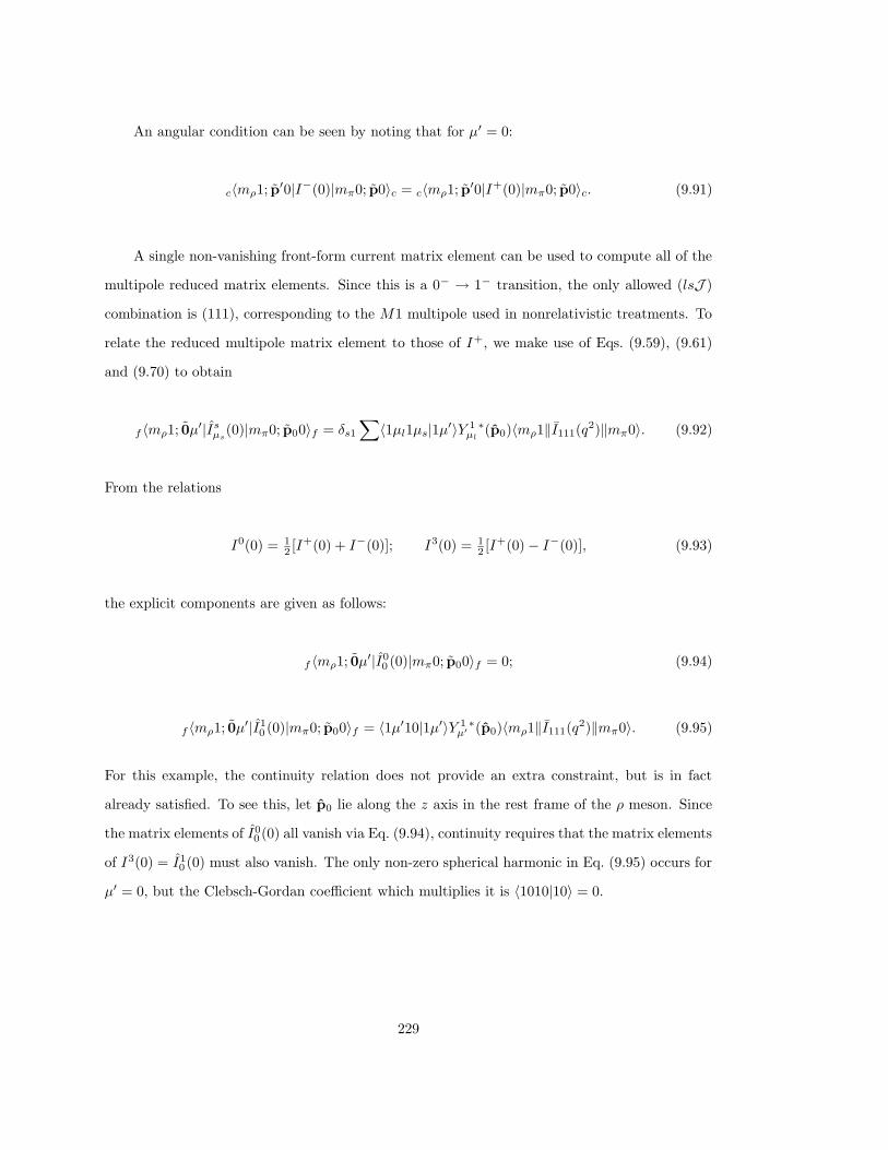
An angular condition can be seen by noting that for µ′ = 0:

c〈mρ1; p′0|I−(0)|mπ0; p0〉c = c〈mρ1; p

′0|I+(0)|mπ0; p0〉c. (9.91)

A single non-vanishing front-form current matrix element can be used to compute all of the

multipole reduced matrix elements. Since this is a 0− → 1− transition, the only allowed (lsJ )

combination is (111), corresponding to the M1 multipole used in nonrelativistic treatments. To

relate the reduced multipole matrix element to those of I+, we make use of Eqs. (9.59), (9.61)

and (9.70) to obtain

f 〈mρ1; 0µ′|Is

µs(0)|mπ0; p00〉f = δs1

∑〈1µl1µs|1µ′〉Y 1

µl

∗(p0)〈mρ1‖I111(q2)‖mπ0〉. (9.92)

From the relations

I0(0) = 12 [I+(0) + I−(0)]; I3(0) = 1

2 [I+(0) − I−(0)], (9.93)

the explicit components are given as follows:

f 〈mρ1; 0µ′|I0

0 (0)|mπ0; p00〉f = 0; (9.94)

f 〈mρ1; 0µ′|I1

0 (0)|mπ0; p00〉f = 〈1µ′10|1µ′〉Y 1µ′

∗(p0)〈mρ1‖I111(q2)‖mπ0〉. (9.95)

For this example, the continuity relation does not provide an extra constraint, but is in fact

already satisfied. To see this, let p0 lie along the z axis in the rest frame of the ρ meson. Since

the matrix elements of I00 (0) all vanish via Eq. (9.94), continuity requires that the matrix elements

of I3(0) = I10 (0) must also vanish. The only non-zero spherical harmonic in Eq. (9.95) occurs for

µ′ = 0, but the Clebsch-Gordan coefficient which multiplies it is 〈1010|10〉 = 0.

229

9.3. Computation of Composite Form Factors

In this section, we consider the ingredients which enter a model calculation of the current

matrix elements 〈p′µ′|Iµ(0)|pµ〉 for composite systems of directly interacting particles. The

treatment of currents runs parallel to the treatment of the direct interactions themselves. The

most general form for the current operator Iµ(x) is

Iµ(x) =∑

i

Iµi (x) +

∑

i<j

Iµij(x) +

∑

i<j<k

Iµijk(x) + · · · . (9.96)

This expansion is analogous to the expansion of the strong-interaction Hamiltonian in terms of

clusters of particles (Po 80). The first term in Eq. (9.96) corresponds to a one-body current,

which acts on each constituent in turn. The second term is the two-body current: by definition it

vanishes if particles i and j are widely separated. The current operator Iµ(x) must obey certain

constraints dictated by special relativity and the continuity equation. These constraints taken

together imply the existence of many-body components in the current operator.

For this approach to be of practical use, Eq. (9.96) should converge rapidly, so that reliable

calculations can be done using one- and two-body current matrix elements only. It is tempting to

go one step further and examine the possibility that observables can be calculated using one-body

current operators alone. This idea has certainly been used extensively in nonrelativistic nuclear

physics. However, as will be seen, the requirements of Poincare invariance impose sufficient

constraints upon electromagnetic current operators that it is impossible to satisfy them all without

many-body components.

In this section, we will show how to construct current matrix elements for calculating elec-

tromagnetic observables. It turns out that the front form has special advantages for this task.

Basic Requirements of Current Operators The combined requirements of Poincare invari-

ance and current conservation imply that the current operator cannot be a sum of the currents of

the single constituent particles. The need for exchange currents to maintain current conservation

was first pointed out by Siegert (Si 37). Siegert assumed that the charge density is a one-body

operator, and then used current conservation to determine a many-body correction to the vector

part of the current to maintain current covariance. Poincare covariance implies that the charge

230

density cannot be a one-body operator. The constraints of Poincare invariance on current oper-

ators has been investigated by Close and Osborn (Cl 70, Cl 71), Coester and Osterbee (Co 75),

Gross (Gr 65, Gr 66a, Gr 66b, Gr 69), Friar (Fr 73, Fr 76), Polyzou (Po 85b), Polyzou and Klink

(Po 88), and Coester (Co 88), and others. This is well known, and has been reviewed extensively

in the contex of exchange currents in (Ch 79, Fr 77, Fr 79 ).

To begin, we examine the constraints of continuity and covariance on the current operators.

Since Iµ(0) is a four-vector operator, it has the same transformation properties as the four

momentum under Lorentz transformations:

U(Λ, a)Iµ(x)U†(Λ, a) = [Λ−1]µνIν(Λx+ a). (9.97)

This implies that

Iµ(x) = e−iP ·xIµ(0)eiP ·x. (9.98)

The commutation relations between Iµ(0) and the Lorentz generators is identical to the commu-

tation relations between the Lorentz generators and the four-momentum:

[Jj(0), Ik(0)]−

= iεjklI l(0); [Jj(0), I0(0)]−

= 0; (9.99)

[Kj(0), Ik(0)]−

= −iδjkI0(0); [Kj(0), I0(0)]−

= −iIj(0); (9.100)

In addition to these equations, the current must satisfy the continuity equation :

[Pµ, Iµ(0)]−

= 0. (9.101)

Equations (9.99)–(9.101) summarize the constraints on the current operator. To understand the

need for exchange currents, we express the current as a sum of one-body and many-body terms:

Assume that the one-body part of the current is covariant with respect to the dynamics of the

231

noninteracting system:

Iµ(0) = Iµ1 (0) + δIµ

ex(0) (9.102)

We assume also that each generator can be expressed as the sum of a non-interacting generator

and an interaction. For example,

K = K1 + δK, (9.103)

and so on for each generator. Inserting these expressions into Eqs. (9.99) and (9.100), we obtain

−iδjkδI0(0) = [δKj(0), Ik(0)]−

+ [Kj1(0), δIk(0)]

−; (9.104)

−iδIj(0) = [δKj(0), I0(0)]−

+ [Kj1(0), δI0(0)]

−. (9.105)

If δK 6= 0, then the right-hand side of both of these equations will not vanish, and thus the current

operator must contain interaction terms. This conclusion holds for instant-form dynamics. In a

front-form dynamics, the interactions come from the rotational commutation relations.

All of these equations can be reduced to a set of equivalent constraints on the charge density

operator. Using Eqs. (9.99) and (9.100), we find that the four-current is uniquely determined by

a knowledge of I0(0) := ρ(0):

Iµ(0) =(ρ,−i[K, ρ]

−

). (9.106)

This equation is a little misleading; it includes a closure sum and thus requires all current matrix

elements. Nevertheless, it is sufficient for our discussion to concentrate on matrix elements of

ρ(0).

Equations (9.99)–(9.101) taken together imply the relations

[H, ρ(0)]−

+ i

3∑

j=1

[P j , [Kj , ρ(0)]−]−

= 0;

[J1(0), ρ(0)]−

= [J2(0), ρ(0)]−

= 0;

[Ki, [Ki, ρ(0)]−]−

+ ρ(0) = 0.

(9.107)

where there is no sum over repeated indices in (9.107).

232

If we use the translation property (9.98) of the current in the continuity relation (9.101), we

obtain

∇ · I(x) − i[H, ρ(x)]−

= 0. (9.108)

This is the form of the continuity equation often encountered in nonrelatistic nuclear physics

(although no nonrelativistic approximation has been made at this point). If the Hamiltonian has

charge-changing pieces (as is the case in nuclear physics with pion exchange) and/or is velocity

dependent, then [H, ρ(x)]−

has two-body components, in which case I(x) must also have two-body

components. This fact has been known for many years. It has often been dealt with by means

of the Siegert hypothesis (Si 37), under which it is assumed that ρ(x) has negligible two-body

matrix elements, and that matrix elements of the commutator in Eq. (9.108) can be evaluated

explicitly to determine any needed matrix elements of I(x).

For Poincare invariant systems, however, the relations (9.107) imply that there must be

two-body currents even if the Hamiltonian is charge neutral and velocity independent. This is a

consequence of the fact that the current is a four-vector, which must transform properly under

boosts and rotations, some of which are interaction dependent. Nevertheless, as will be shown

below, there remain circumstances under which one can calculate matrix elements of certain

components of the current at least approximately, and still maintain a level of consistency with

current continuity and Poincare invariance.

The construction of a suitable current operator is equivalent to finding a charge density

operator which satisfies simultaneously the three conditions (9.107). It is possible to show the

these condition are compatible (Po 85b). They have been manipulated in a variety of ways to

determine leading order relativistic corrections to the current. Many of these attempts involve

expansions in unbounded operators, which are difficult to justify. Moreover, a solution to these

conditions, however difficult it may be to obtain in practice, is not unique. Even if one also

includes the additional constraints of macroscopic locality, it is possible to show with an explicit

counterexample that a solution is not unique.

Another way to understand the relationship between the strong-interaction Hamiltonian and

the current operator is to examine the constraints imposed upon the matrix elements themselves.

233

For canonical spin, the initial hadronic state has the following transformation property:

U(Λ, a)|pµ〉 = eiΛp·a

√ωm(pΛi)

ωm(p)

∑|pΛ µ〉Ds

µµ[Rc(Λ, p)], (9.109)

and the multi-particle final state transforms as follows:

U(Λ, a)|p′1 µ′1 ; · · · ;p′N µ′N(+)〉

= ei∑

iΛp′

i·a∑

|pΛf1µ′1 ; · · · ;pΛfN

µ′N(+)〉

×N∏

i=1

[√ωm′

i(p′Λi)

ωm′

i(p′i)

Ds′

i

µ′

iµ′

i

[Rg(Λ, p′i)]

],

(9.110)

for the final state. In Eq. (9.110), the interacting final state undergoes the same transformation

as a free-particle state. Formally, this is expressed as follows:

U(Λ, a)Ω+ = Ω+

N⊗

i=1

U0i(Λ, a) (9.111)

where U0i(Λ, a) is the free-particle transformation for the ith particle, and

|p′1 µ′1 ; · · · ;p′N µ′N(+)〉 = Ω+|p′1 µ′1; · · · ;p′N µ′N 〉. (9.112)

Equation (9.111) is a consequence of macroscopic locality (Co 82). The covariance condition (9.4)

for current matrix elements becomes:

〈p′1 µ′1 ; · · · ;p′N µ′N(+)|Iµ(x)|pµ〉

= eiΛ(p−∑

ip′

i)·a(Λ−1)µν〈pΛf1

, µ′1, ; · · · ;pΛfNµ′N

(+)|Iν(Λx+ a)|pΛi, µ〉

×N∏

i=1

[√ωm′

i(pΛi)

ωm′

i(pi)

D∗s′

i

µ′

iµ′

i

[Rg(Λ, p′i)]

]√ωm(pΛ)

ωm(p)Ds

µµ[Rg(Λ, p)].

(9.113)

Current conservation gives an additional constraint:

gµν(

N∑

i=1

p′iµ − pµ)〈p1 µ

′1 ; · · · ;p′N µ′N

(+)|Iν(x)|pi µ〉 = 0. (9.114)

While these equations look complicated, they are linear relations. Nevertheless, they represent

a non-trivial set of constraints. The potential difficulty is that the square-root factors and the

234

Wigner rotations depend upon the mass eigenvalue, which is interaction dependent. As we have

already seen, only a subset of current matrix elements is truly independent. All others are related

to a particular subset via the continuity and covariance constraints just given. The problem is

that there are many choices of independent sets of matrix elements, each of which will predict

a complete set of observables for that process. In general, two such sets will predict identical

sets of observables only if the current matrix elements satisfy all of the constraints. A related

conclusion is that the exchange current terms, although always required, are not uniquely fixed

by current conservation or current covariance.

These observations apply to manifestly covariant theories in which the constituents are as-

signed form factors (i.e., non-pointlike vertex functions). The set of form factors must satisfy a

non-trivial set of constraints in order to ensure the overall continuity of the current, but these

constraints do not in turn have a unique solution (Gr 87). These observations apply to other

forms of dynamics as well. In the front form, the non-trivial covariance constraints appear in the

properties of matrix elements under rotations about an axis in the ⊥ plane. Nevertheless, as will

be shown below, there remain circumstances under which one can calculate matrix elements of

certain components of the current at least approximately, and still maintain a level of consistency

with current continuity and Poincare invariance.

Similar arguments can be applied to a Dirac spinor field operator, or any other covariant field

operator. The transformation properties of any such operator is not fully fixed until the dynamics

is defined, and it will in general have many-body or interaction-dependent contributions.

Impulse Approximation As stated above, a common first step in describing currents in com-

posite systems is to describe Iµ as a sum of one-body current operators, i.e., to take only the first

term in Eq. (9.96). While we have already seen that this contribution alone cannot satisfy all of

the combined requirements of continuity and covariance, it is still possible to make a consistent

first approximation using one-body currents only, but only in the front form.

Consider the case of electron scattering from nuclei. In an impulse approximation, the

relevant nuclear matrix element is

〈p′|∑

i

Iµi (0)|p〉 ≈

∑

i

∫d3p′i

∫d3pi 〈p′|p′i〉〈p′i|Iµ

i (0)|pi〉〈pi|p〉. (9.115)

235

For simplicity of illustration, spin indices have been suppressed, and the momentum integrals

have been written generically to represent any form of dynamics. The amplitudes of the form

〈pi|p〉 describe the wave function and the current matrix elements are taken between physical one-

nucleon states, which are in turn connected to the physically observable nucleon form factors.

The calculation is then a matter of integrating wave functions over form factors, just as in the

corresponding nonrelativistic treatment.

The problem is that Eq. (9.115) is not internally consistent in the instant form. This can

be seen as follows. The one-nucleon current information can be summarized as a set of Breit-

frame matrix elements 〈 12q|Iµ(0)| − 1

2q〉. In the integral in Eq. (9.115), the necessary matrix

elements 〈p′|Iµi (0)|p〉 are related to the Breit-frame matrix elements by a Lorentz transformation.

In the instant form, Lorentz transformations are interaction dependent, which implies that a

transformed one-body current matrix element will acquire two-body components. One could

try to avoid this difficulty by using the free-particle matrix elements for all values of p′ and p,

but then the set of matrix elements corresponding to a particular value of q2 will not transform

properly into each other with the interaction-dependent Lorentz transformation. Thus, one-body

currents in the instant form cannot be formulated consistently with respect to Lorentz covariance.

In the front form, this consistency problem can be avoided. As we have seen, for spacelike

momentum transfer, it is possible to find frames in which all invariants can computed from matrix

elements of I+(0) alone. These matrix elements are independent of the choice of frame for a large

class of frames related by the subgroup of front-form boosts. Because the front-form boosts form

a subgroup, the spins remain invariant under front-form boosts. As we will show, if the light front

is oriented so that q+ = 0, then the integral over the Fermi motion only picks up contributions

from subsystem matrix elements related by these kinematic front-form boosts. The result is that

an impulse approximation can be made consistently in any frame with q+ = 0. This can be

demonstrated explicitly in a simple model. Consider a matrix element of I+(0) in a many-body

system:

〈p′|I+(0)|p〉 =

∫dp′1 · · ·

∫dp′n

∫dp1 · · ·

∫dpn〈p′|p′1 · · · p′n〉

× 〈p′1 · · · p′n|I+(0)|p1 · · · pn〉〈p1 · · · pn|p〉.(9.116)

The spin labels have been suppressed, since they do not affect the basic conclusion, as will be

236

discussed below. The initial and final state vectors have the form

〈p1 · · · pn|p〉 = δ(p −n∑

i=1

pi)ψ(p1 · · · pn), (9.117)

where ψ is an n-particle wave function which may differ between initial and final states. The

impulse approximation can be written as follows:

〈p′1 · · · p′n|I+i (0)|p1 · · · pn〉 ≈

n∑

i=1

∏

j 6=i

[δ(p′j − pj)]〈p′i|I+i (0)|pi〉. (9.118)

The integrals over each of the p′i contain a delta function and are trivially eliminated. The net

effect is that each struck particle carries all of the momentum transfer:

〈p′|I+(0)|p〉 ≈∫dp1 · · ·

∫dpn

n∑

i=1

ψ∗(p1 · · · (pi + q) · · · pn)

× 〈pi + q|I+i (0)|pi〉ψ(p1 · · · pi · · · pn),

(9.119)

where q = p′− p. In general, the matrix elements 〈pi + q|I+i (0)|pi〉 appearing inside the integral

depend upon the internal momenta of the target. However, for a specific choice of coordinates,

this matrix element can be factored out of the integral. To see this, consider a front-form boost

for which pi → 0. The final momentum transforms as follows:

(p+i + q+) → m

p+i

(p+i + q+);

(pi⊥ + q⊥) → (pi⊥ + q⊥) − p+i + q+

p+i

pi⊥.(9.120)

In general, the right-hand side of Eq. (9.120) depends upon the Fermi momentum pi. However,

for the special case q+ = 0, we have

(p+i + q+) → m;

(pi⊥ + q⊥) → q⊥.(9.121)

The combined effects of the transformation of the operator I+i (0) and the normalization changes

in the state vectors cancel exactly, with the result:

〈pi + qi|I+i (0)|pi〉 = 〈mq⊥|I+

i (0)|m0⊥〉 (q+ = 0). (9.122)

The current matrix element thus factors out of the Fermi motion integral. This means that for

each momentum transfer q, the impulse approximation depends upon a single one-body current

237

matrix element 〈mq⊥|I+i (0)|m0⊥〉, or, via a different front-form boost, the Breit-frame matrix

element

〈p+ 12q⊥|I

+i (0)|p+ − 1

2q⊥〉, p+ =

√m2 +

1

4q2⊥.

If q+ 6= 0, the one-body matrix elements do not factor out of the integral, and are related to each

other by transformations which include transverse rotations, which are interaction dependent.

Nevertheless, as shown earlier, it is always possible for spacelike momentum transfers to find a

frame in which the condition q+ = 0 is satisfied.

In this example, the spin indices have been suppressed. Had they been included, there would

in general be Wigner rotations associated with the transformation of the one-body current matrix

element, and the argument of the rotation matrices would depend upon the Fermi momentum.

However, for front-form boosts, there are no Wigner rotations, which means that spin-dependent

one-body matrix elements will also factor out of the integral over Fermi motion.

This result marks a major departure from a corresponding calculation in the instant form.

First, the factorization of the matrix element does not occur inside the integral. Second, while

the momentum transfer to the constituent particle in the one-body matrix element is the same,

it must also be related to a Breit-frame matrix element by a Lorentz transformation. However,

the transformations are interaction-dependent, which implies that the set of one-body matrix

elements inside the integral cannot be related to each other in a consistent manner without

introducing two-body current operators. This means that the impulse approximation depends

non-trivially on the choice of frame in which one formulates it.

Example: The π → ρ Transition Form Factor We conclude this section with an illustrative

example. Consider a constituent quark model of the sort discussed in the introductory sections of

this review. We assume that a model of the quark-antiquark system is available with satisfactory

fits to the spectra which include π and ρ mesons. We now obtain an expression for the one-body

current matrix element for the π → ρ transition. As shown above, we need only compute matrix

elements of I+(0). While the angular condition in Eq. (9.91) can only be satisfied through the

use of two-body currents, there is still only one form factor. We therefore assume that matrix

elements of I+(0) have only one-body components, and use them (in fact, we only need one non-

238

vanishing matrix element, as shown in Eq. (9.90)) to calculate the observable. This approach

implies that I−(0) has non-vanishing two-body components, but they need never be calculated.

The starting point is

〈mρ1; p′µ′|I+(0)|mπ0; p0〉

=

∫d2p1⊥dp

+1

∫d2p2⊥dp

+2

∫d2p′1⊥dp

′+1

∫d2p′2⊥dp

′+2

× 〈mρ1; p′µ′|p′1µ′1 p′2µ

′2〉〈p′1µ′1 p′2µ

′2|I+(0)|p1µ1 p2µ2〉

× 〈p1µ1 p2µ2|mπ0; pµ〉.

(9.123)

Only one-body matrix elements of the current are kept:

〈p′1µ′1 p′2µ′2|I+(0)|p1µ1 p2µ2〉 ≈ δµ′

2µ2δ(p′2 − p2)〈p′1µ′1|I+

1 (0)|p1µ1〉

+ δµ′

1µ1δ(p′1 − p1)〈p′2µ′2|I+

2 (0)|p2µ2〉.(9.124)

We now make use of the following state vectors:

|Pk〉 :=

∣∣∣∣∂(p1p2)

∂(Pk)

∣∣∣∣12

|p1µ1 p2µ2〉, (9.125)

The bound-state wave function for the pion is

〈Pkµ1µ2|mπ0; p0〉 =δ(P− p)D( 12 )†

µ1µ1[Rcf (k1)]D

( 12 )†

µ2µ2[Rcf (k2)]

× 〈 12 µ1

12 µ2|1µS〉〈lµl1µS |00〉Y lµl(k)wl

π(k),

(9.126)

and the wave function for the ρ meson is

〈P′k′µ′1µ′2|mρ1; p′µ′〉 =δ(P′ − p′)D

( 12 )†

µ′

1µ′

1[Rcf (k′1)]D

( 12 )†

µ′

2µ′

2[Rcf (k′2)]

× 〈 12 µ′1

12 µ′2|1µ′S〉〈l′µ′l1µ′S |1µ′〉Y l′µ′l(k

′)wl′

ρ (k′)(9.127)

Taking into account the factorization of the one-body current matrix element, as discussed above,

239

we get

〈mρ1; p′µ′|I+(0)|mπ0; p0〉

≈ e1e〈p+ 1

2q⊥µ′1|I+(0)|p+ − 1

2q⊥µ1〉∫d2p2⊥dp

+2

(2π)3

∣∣∣∣∂(p′1p2)

∂(p′k′)

∣∣∣∣12∣∣∣∣∂(p1p2)

∂(pk)

∣∣∣∣12

×D( 12 )

µ1µ1[Rcf (k′1)]D

( 12 )

µ2µ2[Rcf (k′2)]

× 〈 12 µ′1

12 µ′2|1µ′S〉〈lµ′l1µ′S |1µ′〉Y l′µ′l(k

′)wlρ(k′)

×D( 12 )†

µ1µ1[Rcf (k1)]D

( 12 )†

µ2µ2[Rcf (k2)]

× 〈 12 µ1

12 µ2|1µS〉〈lµl1µS |00〉Y lµl(k)wl

π(k)

+ [1 ↔ 2]; (p+ =

√m2 +

1

4q2⊥).

(9.128)

240

10. Relation to Covariant Theories

The purpose of this section is to exhibit the relationship between relativistic particle dynam-

ics formulated on a Hilbert space of square integrable functions, manifestly covariant quantum

mechanical models, and covariant quantum field theory. For the case of a free particle, all three

formulations are shown to be equivalent. Interactions can be considered as perturbations of

non-interacting models. The problem of adding interactions in each of these cases is considered

briefly.

To exhibit the relation between these three descriptions of a free particle, we construct

transformations that relate state vectors in each of these representations, while preserving all

transition probabilities. We do this for the case of a spin- 12 Dirac particle.

We begin with a free particle of mass m and spin 12 , corresponding to the general construction

in Section 4. The Hilbert space for this particle is an irreducible representation space of P

corresponding to mass m and spin 12 , namely, the space of square integrable functions of three

components of the linear momentum and a magnetic quantum number associated with spin 12 .

The scalar product is

〈f |g〉 :=

12∑

µ=− 12

∫d3p 〈pµ|f〉∗〈pµ|g〉, (10.1)

where

〈f |f〉 <∞. (10.2)

These states transform irreducibly under P :


√ωm(pΛ)

ωm(p)

∑|pΛ µ〉D

12µµ[Rc(Λ, p)]. (10.3)

To construct a field satisfying canonical equal-time (anti-) commutation relations, we must also in-

troduce the corresponding antiparticle. Since the mass and spin fix the transformation properties

of an irreducible representation of the Poincare group, and the mass and spin of the antiparticle

are the same as the mass and spin of the particle, we can assume that antiparticle states have

241

the same transformation properties under U(Λ, a) as particle states. We use the notation |pµ〉

to denote a pure state of the antiparticle with momentum p and magnetic quantum number µ.

The transformation properties of the antiparticle states are


√ωm(pΛ)

ωm(p)

∑|pΛ µ〉D

12µµ[Rc(Λ, p)]. (10.4)

To construct a field of spin 12 that transforms covariantly under U(Λ, a), we introduce a

Poincare invariant vacuum |0〉, satisfying

U(Λ, a)|0〉 = |0〉 (10.5)

and

〈0|0〉 = 1, (10.6)

together with abstract creation operators a†(p, µ) for particle states, and b†(p, µ) for antiparticle

states. These operators create the particle and antiparticle states from the vacuum:

a†(p, µ)|0〉 = |pµ〉; (10.7)

b†(p, µ)|0〉 = |pµ〉. (10.8)

The creation operators and their adjoints are assumed to satisfy canonical anticommutation

relations:

a(p′, µ′), a†(p, µ) = δµ′µδ(p′ − p). (10.9)

This fixes the statistics of multiparticle states and the normalization of the one-body states.

The vacuum is annihilated by the adjoints of the creation operators:

a(p, µ)|0〉 = 0 b(p, µ)|0〉 = 0. (10.10)

The transformation properties of the creation operators are fixed by Eqs. (10.3), (10.4),

(10.5), (10.7) and (10.8), and the property that U(Λ, a) acts irreducibly on the one-particle and

242

one-antiparticle subspaces. These properties are given as follows:

U(Λ, a)a†(pµ)U†(Λ, a) = eiΛp·a

√ωm(pΛ)

ωm(p)

∑a†(pΛ µ)D

12µµ[Rc(Λ, p)]; (10.11)

U(Λ, a)b†(pµ)U†(Λ, a) = eiΛp·a

√ωm(pΛ)

ωm(p)

∑b†(pΛ µ)D

12µµ[Rc(Λ, p)]. (10.12)

The transformation properties of a(p, µ) and b(p, µ) follow by taking adjoints of Eqs. (10.11)

and (10.12):

U(Λ, a)a(pµ)U†(Λ, a) = e−iΛp·a

√ωm(pΛ)

ωm(p)

∑a(pΛ µ)D

12∗µµ [Rc(Λ, p)] (10.13)

U(Λ, a)b(pµ)U†(Λ, a) = e−iΛp·a

√ωm(pΛ)

ωm(p)

∑b(pΛ µ)D

12∗µµ [Rc(Λ, p)]. (10.14)

It is useful to rewrite Eqs. (10.13) and (10.14) using

D12∗µµ [Rc(Λ, p)] = D

12µµ[R−1

c (Λ, p)], (10.15)

which gives

U(Λ, a)a(pµ)U†(Λ, a) = e−iΛp·a

√ωm(pΛ)

ωm(p)

∑D

12µµ[R−1

c (Λ, p)]a(pΛ µ); (10.16)

U(Λ, a)b(pµ)U†(Λ, a) = e−iΛp·a

√ωm(pΛ)

ωm(p)

∑D

12µµ[R−1

c (Λ, p)]b(pΛ µ). (10.17)

We now use the property that the conjugate representations of SU(2) are equivalent:

Ds∗µ′µ(R) =

∑Ds

µ′µ′(R−1y )Ds

µ′µ(R)Dsµµ(Ry), (10.18)

where

Ry = exp(− 12 iπσ2) = −iσ2, (10.19)

to transform b†(p, µ) so that it has the same transformation properties as a(p, µ). Relation

(10.18) follows because a similarity transformation by any multiple of σ2 is equivalent to a complex

243

conjugation of an SU(2) matricex. This extends to the D functions because they are polynomials

in the SU(2) matrix elements with real coefficients, as defined in Eq. (4.14). It follows that the

combination

s∑

µ′=−s

D12

µµ′(Ry)b†(p, µ′) (10.20)

has the same transformation properties as a(p, µ) and b(p, µ) under U(Λ, a).

There are two ways to construct a covariant field operator. One method is to define the op-

erator in terms of its matrix elements in a complete set of states that transform irreducibly under

P . The transformation properties of the states and the field allow us to use the Wigner-Eckart

theorem for P to express these matrix elements of the field operator as a sum of Clebsch-Gordan

coefficients (for P) and some invariants, which can be fixed by local commutation relations, choice

of spinor representation, and parity. This is exactly how we treated current operators in the pre-

vious section. The second is to assume that the field Ψ(x) is a spinor-valued linear combination

of a(p, µ) and b†(p, µ), and determine the coefficients from covariance, locality and parity. The

two approaches are equivalent.

We begin by assuming the following decomposition:

Ψa(x) =∑∫

d3p[ua(p, µ)a(p, µ)e−i(ωm(p)t−x·p)

+ va(p, µ)Dsµµ(Ry)b†(p, µ)ei(ωm(p)t−x·p)

],

(10.21)

where ua(p, µ) and va(p, µ) are to be determined. The function D12µµ(Ry) is included for conve-

nience. It could easily be absorbed into the definition of va(p, µ) or b†(p, µ). We assume that

this field transforms covariantly under the action of U(Λ, a):

U(Λ, a)Ψa(x)U†(Λ, a) = S(Λ−1)aa′Ψa′(Λx+ a), (10.22)

where S(Λ)aa′ is a finite dimensional representation of SL(2, C) which defines the type of field.

For a Dirac particle, S(Λ) is, up to a similarity transformation, the direct sum of a right- and

244

left-handed representation of SL(2, C):

SDirac(Λ)aa′ =

(Λ 0

0 (Λ†)−1

)

aa′

. (10.23)

In order to find equations that fix the spinor wave functions ua(p, µ) and va(p, µ), we evaluate

Eq. (10.22) using the transformation properties of a(p, µ) and b†(p, µ), and equate coefficients

of a(p, µ) and b†(p, µ). The result is

∑ua(pΛ, µ)D

12µµ[Rc(Λ, p/m)] =

∑S(Λ)aa′ua′(p, µ)

√ωm(p)

ωm(pΛ); (10.24)

∑va(pΛ, µ)D

12µµ[Rc(Λ, p/m)] =

∑S(Λ)aa′va′(p, µ)

√ωm(p)

ωm(pΛ). (10.25)

Equations (10.24) and (10.25) show that these coefficients change finite-dimensional representa-

tions of SL(2, C) into Wigner rotations associated with a given momentum and Lorentz trans-

formation. The p dependence of the wave functions is fixed by covariance. To see this, let

(Λ,p) → (Lc(p/m),0) in Eqs. (10.24) and (10.25). In this case, the Wigner rotation becomes the

identity:

ua(p, µ) = S[Lc(p/m)]aa′ua′(0, µ)

√m

ωm(p); (10.26)

va(p, µ) = S[Lc(p/m)]aa′va′(0, µ)

√m

ωm(p). (10.27)

This fixes the p dependence of these wave functions in terms of their value when p = 0. To

determine the rest wave functions, we consider the case that Λ = R is a rotation, which leaves

p = 0 invariant:

ua(0, µ) = S(R)aa′ua′(0, µ′)Dsµ′µ(R−1); (10.28)

va(0, µ) = S(R)aa′va′(0, µ′)Dsµ′µ(R−1). (10.29)

For an infinitesimal rotation about the z axis, these equations become eigenvalue relations:

∑

a′

δSzaa′ua′(0, µ) = −iµua(0, µ); (10.30)

245

∑

a′

δSzaa′va′(0, µ) = −iµva(0, µ), (10.31)

where

δSzaa′ =

d

dθSaa′(e

i2 θσz )

∣∣∣θ=0

. (10.32)

For the case of a Dirac spinor,

δSzaa′ = − i

2

1 0 0 0

0 −1 0 0

0 0 1 0

0 0 0 −1

, (10.33)

which is already diagonal. In particular, we have

ua(0, 12 ) = va(0, 1

2 ) =

c

0

d

0

; (10.34)

ua(0,− 12 ) = va(0,− 1

2 ) =

0

e

0

f

, (10.35)

where c, d, e and f are independent constants. In SL(2, C), space reflection implies that Λ ↔

(Λ†)−1, which interchanges the upper and lower components of these spinors. This was discussed

in the previous section on tensor operators. It also changes the sign of D12

µµ′(Ry), and does

nothing to the creation or annihilation operators when p = 0. Thus, if we want the Dirac field

to be invariant under spatial reflection, we find that

c

0

d

0

=

d

0

c

0

;

0

e

0

f

=

0

f

0

e

(10.36)

246

for ua(0, µ), and

c

0

d

0

= −

d

0

c

0

;

0

e

0

f

= −

0

f

0

e

(10.37)

for va(0, µ), since va(0, µ) is multiplied by D12

µµ′(Ry). If we combine Eqs. (10.34)–(10.37), we

obtain

ua(0, 12 ) = C

1

0

1

0

; ua(0,− 12 ) = C

0

1

0

1

; (10.38)

va(0, 12 ) = C

1

0

−1

0

; va(0,− 12 ) = C

0

1

0

−1

. (10.39)

The constants are determined by the requirement

Ψa(x),Ψ†b (y)|x0=y0

= δabδ(x − y). (10.40)

This is the only part of the development which cannot be completed without including the

antiparticle. The commutation relations (10.40) imply the normalization

C =1√

2(2π)32

(10.41)

for each of the four spinor amplitudes. Thus, the conditions of covariance, parity and equal-time

anticommutation relations fix the form of this field uniquely, up to phase and degeneracies. The

247

results are

u(p, µ) =m− γ · p√

2ωm(p)(m+ ωm(p))u(0, µ); (10.42)

v(p, µ) =m+ γ · p√

2ωm(p)(m+ ωm(p))v(0, µ), (10.43)

where

γ0 =

(0 I

I 0

)γ =

(0 −σ

σ 0

). (10.44)

Note that the representation of the Dirac γ matrices was determined by the choice of represen-

tation of S(Λ)aa′ in Eq. (10.25).

With these wave functions, the field operator Ψa(x) is an ordinary Dirac field. In most

modern treatments, the factor D12µµ(R−1

y ) is absorbed in the definition of b†(p, µ). Our discussion

follows that of Weinberg (We 65), where this factor appears explicitly.

Note that the index a on the spinor wave function transforms under a finite-dimensional

representation of SL(2, C), while the index µ transforms under a unitary representation of the

little group (SU(2)) of a positive-energy, positive-mass irreducible representation of P . In SU(2),

the fundamental representation is self-conjugate, while this is not the case for finite-dimensional

representations of SL(2, C). This is why four-component spinors are needed to construct Lorentz

covariant fields, but not for the creation and annihilation operators.

To find the transformation that relates the field description to the particle description, it is

convenient to compute the Fourier transform of the adjoint field applied to the vacuum:

Ψ†a(p)|0〉 = (2π)−2

∫d4x e−ip·xΨ†

a(x) = (2π)2u∗a(p, µ)a†(p, µ)|0〉δ(p0 − ωm(p)). (10.45)

We use the relation

a†(p, µ)|0〉δ[p0 − ωm(p)] = 2πΨ†(p)|0〉γ0u(p, µ), (10.46)

which follows from Eq. (10.45) by using the following:

u†(p, µ)γ0u(p, ν) = (2π)−3δµν . (10.47)

Vectors in the field and particle case can be expressed in terms of functions ga(p) and f(p, µ),

248

respectively, by using

|ξ〉 =

∫d4p Ψ†

a(p)|0〉ga(p); (10.48)

|ξ〉 =

∫d3p |pµ〉f(p, µ). (10.49)

From Eqs. (10.45) and (10.46), we obtain the following relation between the functions that define

the same vector in the particle and the field cases, respectively:

f(p, µ) = (2π)−2u†a(p, µ)ga(ωm(p),p); (10.50)

ga(p)|p0=ωm(p) = (2π)(γ0u(p, µ))af(p, µ). (10.51)

The correspondence f(p, µ) ↔ ga(p)|p0=ωm(p) is a norm preserving correspondence between

square integrable wave functions of the particle theory and the equivalence class of covariant wave

functions that agree on the physical mass shell of the particle. Since covariant wave functions that

vanish on the physical mass shell correspond to zero-norm states, by Eq. (10.45), the equivalence

classes of covariant functions that agree on the mass shell correspond to physical states of the field

theory. It follows that the correspondence f(p, µ) ↔ ga(p)|p0=ωm(p) is a unitary correspondence

between one-particle states of the particle theory and physical one-particle states of the field

theory. There is a similar correspondence between the two representations of the antiparticles.

We let W denote the unitary mapping that takes a particle state to the corresponding state in the

field theory. This shows that free particles in a particle theory and a field theory differ only by

a change of representation. Antiparticles were not needed to construct covariant fields – only to

obtain the canonical anticommutation relations. Antiparticles are easily included in the particle

theory if desired.

Next, we consider an equivalent quantum mechanical theory with covariant wave functions.

This will be done using the field theory. The covariance of the field and the unitarity of U(Λ, a)

249

implies the following:

∫d4x

∫d4y g∗a(x)〈0|Ψa(x)Ψ

†b (y)|0〉fb(y)

=∑∫

d4x

∫d4y g∗a(x)S(Λ)aa′

× 〈0|Ψa′(Λ−1(x− a))Ψ†b′(Λ

−1(y − a))|0〉S†(Λ)b′bfb(y)

=∑∫

d4x

∫d4y g∗a(Λx+ a)S(Λ)aa′

× 〈0|Ψa′(x)Ψ†b′(y))|0〉S†(Λ)b′bfb(Λy + a).

(10.52)

Under the transformations

fb(x) → f ′b(y) =∑

S†(Λ)bb′fb′(Λy + a); (10.53)

g∗a(x) → g′∗a (y) =∑

g′∗a′(Λy + a)S(Λ)a′a, (10.54)

the scalar product defined by Eq. (10.52) is invariant. Thus, ga(x) and fa(x) can be interpreted

as covariant wave functions on a Hilbert space, where the scalar product is defined in terms of

the kernel

K(x, y)ab = 〈0|Ψa(x)Ψ†b (y)|0〉. (10.55)

Direct computation of this kernel yields

K(x, y)ab =

∫d4p

(2π)32mδ(p2 +m2)e−ip·(x−y)Θ(p0)Λ+(p)ab, (10.56)

where Λ+ab is an orthogonal projector on the subspace of the four-component spinor space spanned

by the u’s. In momentum space this kernel restricts two covariant wave functions to the positive-

energy mass hyperbola, and projects the spinor indices on the space spanned by the u-spinors.

How these functions behave away from the positive-energy mass hyperbola and in the subspace

spanned by the v-spinors has no effect on this scalar product. Thus, although the wave functions

ga(p) transform covariantly, a state corresponds to an equivalence class of these functions whose

difference has zero norm in the semi-scalar product defined by Eq. (10.56). There is a similar

kernel associated with the antiparticles.

250

The property of having a quantum mechanics with a non-trivial scalar product is character-

istic of all relativistic quantum models with wave functions that (1) are probability amplitudes

and (2) transform covariantly (Po 85a).

The correspondence (10.50) and (10.51) gives the connection between this covariant free

particle quantum mechanics and the quantum theory of free particles that began this section. As

in the case of fields, the correspondence can be realized as a unitary change of representation.

We have shown the equivalence of the description of a free particle in a particle theory, a

field theory, and a theory with covariant wave functions.

In all three of these approaches, it is possible to add interactions. We have discussed inter-

actions for the case of the particle theory. In a field theory, interactions are generally added in a

manner which is designed to preserve microscopic locality, usually with a Lagrangian. It can also

be done alternatively by directly adding interactions to the Poincare generators of the free field

(We 65). In a covariant quantum theory, interactions involve modifications of the scalar prod-

uct. Although it is possible to develop the connections in the case that interactions are present,

these connections are not really in the spirit of how the different models are used in practice.

For instance, it is possible to formulate successive approximations to a local field theory, where

each term is a particle model with a finite number of degrees of freedom satisfying macroscopic

locality. If one took seriously the interactions derived in such an approach, it is unlikely that

they would be as good as a purely phenomenological one, for the obvious reason that some of the

physics contained in excluded degrees of freedom can be recovered by fitting parameters to data.

A similar situation occurs if one applies the Bethe-Salpeter equation to a theory of nucleons and

pions. It is only after one includes enough mesons, and fits all of the various parameters to phase

shifts, that one obtains a sensible model.

In the case of a free particle, the connections between the three approaches can be made

precise, and they provide a good starting point for a general understanding of the relation between

these three approaches.

Models with covariant wave functions with probability interpretations arise in an alternative

relativistic formulation of quantum mechanics called covariant constraint dynamics. This ap-

proach is discussed extensively elsewhere (Lo 87). We can think of a two-particle system with the

251

four-momentum of each particle restricted to its positive-energy mass hyperbloid. The two-body

wave function is a covariant wave function in eight variables, subject to two covariant (mass shell)

constraints. In this case, the constraints commute. They can be used to construct a kernel of a

covariant scalar product (as above), or, equivalently, they can be realized as a pair of compatible

equations that must be satisfied by the two-body wave function. To include interactions, either

the constraints or the kernel of the scalar product is perturbed in a manner that preserves the

compatibility of the constraints and the covariance, or, equivalently, the covariance and the Her-

miticity of the kernel of the scalar product. The problem is to find covariant interactions which

are compatible, satisfy cluster properties, and also satisfy the spectral condition.

The relation to a model satisfying macroscopic locality and not microscopic locality is an

approximation at best. One way the treat this problem is to eliminate degrees of freedom from

the generators in an manner that preserves the Lie algebra. This has been done perturbatively

(Gl 81).

We close this section with some brief comments about “covariant wave functions” associated

with the Bethe-Salpeter equation (Sa 51). In most treatments of quantum field theory, bound

states are described by the Bethe-Salpeter equation or a related reduction. These have been both

discussed and applied extensively in the literature (Bl 60, Bl 66, Gr 82a, Gr 82b). A discussion

of this approach is not within the scope of this paper, but there are some important points that

merit discussion. The first is that the “covariant wave functions” of the Bethe-Salpeter equation

are not wave functions in the sense of probability amplitudes (i.e., there is no associated scalar

product that is positive semi-definite ). Instead, they are more closely related to the current

matrix elements discussed in the previous section. They are matrix elements of covariant field

operators evaluated between physical states. They are sometimes confused with wave functions

because it is possible to construct quadratic functions involving these amplitudes to evaluate

matrix elements of any operator (Ma 55, Hu 75). Although the Bethe-Salpeter equation is

motivated by field theories, in applications the kernel is approximated . When the approximate

kernel does not have all of the properties of the exact theory, such as crossing symmetry, then

these models violate microscopic locality. In addition, in realistic applications, the kernel is

treated phenomenologically. Under these conditions, Bethe Salpeter methods resemble, in spirit,

the methods discussed in this paper in the sense that they are phenomenologies that satisfy

252

macroscopic locality but not microscopic locality. As a practical matter, the dynamical equations

are more difficult to solve, and a normalization condition is needed to extract physical matrix

elements.

253

11. Conclusion

Our goal in this review has been to provide both a formal foundation and a set of tools

for constructing relativistic quantum mechanical models in nuclear and particle physics. Rather

than simply summarizing a paper of this size, we attempt here to highlight what we believe to

be the most important points.

We have devoted considerable space to the topic of relativistic invariance and its implications

for the construction of quantum mechanical models. A key element of this discussion is that there

are many ways of making relativistic models. While relativistic invariance can certainly eliminate

models on the basis of some sort of inconsistency, it serves more as a constraint than as a pointer

to some specific theory. Thus, the choice of model must in general be made on other grounds,

such as the complexity of the interaction and/or the number of parameters needed to describe a

set of observables, or the ability to perform accurate and convergent calculations.

One consequence of the variability of models is that it is impossible to isolate a unique

“relativistic correction.” Different models may have the same nonrelativistic limit, or different

limits, depending in detail on how such a limit is taken.

Another element which distinguishes relativistic models is that of locality. The models

featured in this review can be made to satisfy macroscopic locality–a property seen in experiments

and therefore, in our view, necessary for any model. To go beyond this and require a theory to

satisfy microscopic locality, as in a local field theory, is certainly sufficient, but not necessary. The

price paid for this in some instances can be a theory with an infinite number of degrees of freedom

and a large coupling constant, for which few (if any) accurate and/or convergent calculations can

be made. Furthermore, attempts to approximate such a theory can easily result in the loss

of microscopic locality, in addition to macroscopic locality, or even the relativistic invariance

which motivated the theory in the first place. Thus, while local quantum field theory has had

certain highly visible successes, it does not represent the required path to combining relativity and

quantum mechanics, and in some cases, particularly those involving strong interactions and/or

phenomenology, it may not be the desired path.

254

Light-front dynamics occupies a special place in our discussion. The fact that it is imple-

mented with only three out of ten interacting Poincare generators (as opposed to four out of

ten in the instant form) makes it possible to do a number of practical calculations with Lorentz

transformations involving only kinematic generators. For instance, it permits one to determine

the spin transformation properties of purely phenomenological wave functions under front-from

boosts. It is especially useful for the evaluation of current matrix elements. For spacelike momen-

tum transfer, it is possible in light-front dynamics to make a consistent impulse approximation

(which is not possible in the instant form) whereby all observables can be consistently calculated

from matrix elements of a single component of the relevant current operator in set of frames

related by a subgroup of front-form Lorentz transformations.

We have not provided detailed discussion of specific applications, except as illustrative ex-

amples. As stated above, our goal has been to provide enough tools for the interested reader to

digest the literature and to perform new calculations which advance the field. While citations

to specific published studies have been provided (see the end of Section 2.1), we provide here a

general view of the current status of the literature.

Most calculations to date which use direct interations have centered on systems involving

two or three nucleons, or two or three quarks. While there have been calculations which make

explicit comparisions to data, there are many more observables yet to be studied. These in-

volve both pure strong-interaction processes in few-body systems as well as reactions involving

an electromagnetic or weak probe. With new high-intensity, high-duty-factor machines becom-

ing a reality in energy regions where relativistic kinematics are clearly important, the need for

detailed relativistic models is not an idle one. Models of the type presented in this review require

calculations which are certainly more intensive than their nonrelativistic counterparts, but many

are within the capabilities of modern supercomputers or even workstations.

On the formal side, the need to construct realistic models with particle production which

also satisfy macroscopic locality has been partially satisfied, but there is more work to be done.

The general problem of making models which allow the production of arbitrary numbers of

particles must also be addressed by calculations based upon field theory: while one can make

exact statements in the latter case, specific (truncated) models raise the same sort of questions.

255

There is also the need to isolate and understand ways to implement a reliable relativistic

quantum many-body problem. While an explicit formulation satisfying macroscopic locality is

available in the approach described in this review (see So 77 or Co 82), it is neither workable

nor desirable for large numbers of particles, any more than a nonrelativistic version would be.

A first approach would then be to try to utilize approximations which have proven reliable in

nonrelativistic nuclear physics. Of course, the word “reliable” implies an accompanying justifi-

cation that corrections are small, and not that a certain step was taken in the face of prohibitive

computational complexity. Relativistic models based upon any other approach must also address

this issue.

We have not attempted to discuss in any detail the other approaches to relativistic quantum

mechanics which now exist in the literature. A comparative discussion of the distinctive features

of each approach would require enough extra technical machinery as to make this review unman-

ageable. These different approaches sit at various stages of advancement. Beyond relativistic

invariance, key elements that models must address successfully include macroscopic locality and

the spectral condition. In addition, since many other implementations are formulated in terms of

transition operators, it must also be shown that there is an underlying quantum theory. These

questions have been worked out for certain approaches and/or certain applications, but there is

certainly room for many contributions.

256

Acknowledgements

The work behind this review was supported in part by grants PHY-8818836 from the National

Science Foundation (BDK) and DE-AC02-81ER40038 from the Department of Energy (WNP).

We wish to thank Dr. F. Coester for many discussions which have contributed materially to the

content of this review.

257

APPENDIX A

Scattering Theory

In this Appendix, we provide an overview of various aspects of scattering theory as they

relate to relativistic models. Time-dependent treatments of scattering employ time development

operators involving the Hamiltonian. In this review, it was convenient to utilize operators other

than the Hamiltonian (such as the mass M or its square, or the front-form Hamiltonian P−)

to formulate the scattering problem. We have therefore included a derivation of the relation

among the S and T operators and the differential cross section, along with a discussion of the

invariance principle (Bi 62, Ka 65, Ch 76, Ob 78), and a discussion concerning the construction of

phenomenological interactions fit to nucleon-nucleon scattering data. Our purpose is to provide

the justification for these alternate formulations of the scattering problem. Although all of this

material can be found in the literature, it is difficult to find it in one place.

In addition, we show that for any of the forms of dynamics covered in this review, it is

possible to take advantage of two-body potentials which have been fit to scattering data using

the Schrodinger equation. This property was discussed in the front-form examples in Section 2,

but it is in fact more general

A.1. The Relation Between S and T

For models with a finite number of degrees of freedom, the multichannel scattering operator

is defined in terms of channel wave operators as:

Sβα := Ω†β+Ωα− (A.1)

where a is a partition of N particles into na clusters, and the partition wave operators are defined

by

limt→∞

‖Ωα±|Ψα〉 − e±iHte∓iHat|Ψα〉‖ = 0. (A.2)

In equation (A.2), α denotes a channel in which the particles in each cluster of the partition a

are separately bound. Ha is the partition Hamiltonian, which is obtained from the original

258

Hamiltonian by turning off all interactions between particles in different clusters of the partition

a. The partition Hamiltonian is also the sum of the subsystem Hamiltonians for each cluster in

a:

Ha =

na∑

i=1

Hai. (A.3)

There is a scattering channel α associated with the partition a if each of theHaihas a bound state.

Let |αi pi〉 denote a bound state of Haicorresponding to the channel α with total momentum

pi. Now define the channel projection operator:

Πα :=

∫ na∏

i=1

d3pi|p1 α1 · · ·pnaαna

〉〈p1 α1 · · ·pnaαna

|. (A.4)

The channel states |Ψα〉 are normalizable vectors satisfying:

|Ψα〉 = Πα|Ψα〉. (A.5)

Note that a given partition a may have none or many associated scattering channels α.

To construct formulas for scattering matrix elements, let α and β denote scattering channels

associated with the asymptotic partition Hamiltonians Ha and Hb, respectively. Let |α〉 and |β〉

denote sharp eigenstates of the partition Hamiltonians:

Ha|α〉 = Eα|α〉; Hb|β〉 = Eβ |β〉. (A.6)

Using Eqs. (A.1) and (A.2), the S-matrix elements can be evaluated as follows:

〈β|Sba|α〉

= limt→∞

〈β|eiHbte−2iHteiHat|α〉

= 〈β|α〉 + limt→∞

t∫

0

dt′d

dt′〈β|ei(Eβ+Eα−2H)t′ |α〉

= 〈β|α〉 + limε→0+

i

∞∫

0

dt′ 〈β|[(Eβ −H)ei(Eβ+Eα−2H+iε)t′

+ ei(Eβ+Eα−2H+iε)t′(Eα −H)]|α〉

= 〈β|α〉 + limε→0+

12 〈β|

[(H − Eβ)

1

E −H + iε+

1

E −H + iε(H − Eα)

]|α〉,

(A.7)

where E = 12 (Eα +Eβ) is the average energy of the initial and final asymptotic states. Equation

259

(A.7) is interpreted as the kernel of an integral operator. S-matrix elements are obtained by

integrating the sharp eigenstates in Eq. (A.7) over normalizable functions of the energy and any

other continuous variables. To simplify this expression, we introduce a more compact notation.

The residual interactions V a and V b are defined as follows:

V a := H −Ha; V b := H −Hb, (A.8)

where

V a|α〉 = (H − Eα)|α〉; V b|β〉 = (H − Eβ)|β〉. (A.9)

We introduce resolvent operators of the Hamiltonian and the partition Hamiltonian:

R(z) :=1

z −HRa(z) :=

1

z −Ha. (A.10)

These operators satisfy the second resolvent relations (Hi 57):

R(z) −Ra(z) = Ra(z)V aR(z) = R(z)V aRa(z). (A.11)

If these identities are used in Eq. (A.7), we get

〈β|S|α〉

= 〈β|α〉 + limε→0+

12 〈β|

[V b(1 + R(E + iε)V a

)Ra(E + iε)

+Rb(E + iε)(1 + V bR(E + iε)

)V a]|α〉

= 〈β|α〉[1 − lim

ε→0+

Eβ − Eα

Eβ − Eα + 2iε

]

+ limε→0+

[1

Eβ − Eα + 2iε+

1

Eα − Eβ + 2iε

]〈β|(V a + V bR(E + iε)V a

)|α〉

= 〈β|α〉 limε→0+

[2iε

Eβ − Eα + 2iε

]

+ limε→0+

[ −4iε

(Eβ − Eα)2 + 4ε2

]〈β|(V a + V bR(E + iε)V a

)|α〉.

(A.12)

It is now possible to evaluate the limit as ε → 0. It is important to remember that this is the

kernel of an integral operator.

260

The first term in square brackets is unity when the initial and final energies are identical,

and zero otherwise; however, the limit in the bracket is a Kronecker delta and not a Dirac delta

function. For a 6= b, we expect that 〈β(E ′)|α(E)〉 will be Lebesgue measurable in E ′ for fixed

E, so there is no contribution from the first term in Eq. (A.12). For the case that Hb = Ha, we

have 〈β(E′)|α(E)〉 ∝ δ(E′ − E). The matrix elements vanish by orthogonality unless Eβ = Eα,

but then coefficient is unity. Thus, the first term is 〈β|α〉 if the initial and final channel are the

same, but zero otherwise. Note that the matrix elements vanish by orthogonality for two different

channels governed by the same asymptotic Hamiltonian with the same energy. The first term in

(A.12) is therefore a channel delta function.

For the second term, the quantity in square brackets becomes −2πiδ(Eβ −Eα), which leads

to the relation

〈β|S|α〉 = 〈a|b〉δβα − 2πiδ(Eβ − Eα)〈β|T ba(Ea + i0+)|α〉, (A.13)

where

T ba(z) = V a + V bR(z)V a. (A.14)

This is the general expression for the transition operator in a multichannel scattering theory.

It applies both to relativistic and to nonrelativistic applications. The multichannel transition

operator T ab(z) must be constructed in a dynamical model.

In models where the residual interactions and the resolvent commute with the total linear

momentum operator, and if the sharp channel states |α〉 and |β〉 are simultaneous eigenstates of

the appropriate partition Hamiltonian and the linear momentum, then the delta function can be

factored out of the matrix element:

〈β|T ba(Ea + i0+)|α〉 = δ3(pβ − pα)〈β‖T ba(Ea + i0+)‖α〉. (A.15)

If this is used in Eq. (A.13), then the S-matrix elements can be expressed in terms of the reduced

transition operators as follows:

〈β|S|α〉 = 〈a|b〉δβα − i(2π)δ4(pβ − pα)〈β‖T ba(Ea + i0+)‖α〉 (A.16)

This expression has the advantage that the delta function is manifestly invariant under Poincare

261

transformations. The factor (2π)3 is included by convention.

For relativistic models of the type discussed in this review, there are cases where the residual

interactions and resolvent commute with the system four-velocity or the light-front components

of the four-momentum, rather than the three-momentum. In general, let g = g(p; p0) be three

independent functions of the four-momentum that commute with the residual interactions and

the resolvent. Then Eq. (A.15) can be replaced by the following:

〈β|T ba(Ea + i0+)|α〉

=: δ3(gβ − gα)

∣∣∣∣∣∂g(p, p0

β)

∂p

∣∣∣∣∣

12 ∣∣∣∣∂g(p, p0

α)

∂p

∣∣∣∣

12

〈β‖T ba(Ea + i0+)‖α〉.(A.17)

The Jacobian factors can always be absorbed into the definition of the reduced matrix element.

Thus, we can write

δ4(pα − pβ) = δ(Eα − Eβ)δ3(pα − pβ) = δ(Eα − Eβ)δ3(gβ − gα)

∣∣∣∣∂g(p, p0

α)

∂p

∣∣∣∣ , (A.18)

and this yields

〈β|S|α〉 = 〈a|b〉δβα − i(2π)δ4(pβ − pα)〈β‖T ba(Ea + i0+)‖α〉. (A.19)

In what follows, this convention is used to define the reduced matrix element.

A.2. The Invariance Principle

In relativistic problems, it is convenient to utilize a more general form of the transition

operator. In applications, we have replaced H by a non-trivial function f(H,p) of the four-

momentum, such as M , M2, P−, ( 14M

2 − m2), and other operators, and then formulated the

scattering problem. The justification for this is the Kato-Birman invariance principle (Bi 62, Ka

66, Ch 76, Ob 78) for wave operators, and the dominated convergence theorem. The invariance

principle is a rigorous result, whereby it is possible to replace H, Ha and Hb in Eq. (A.2) by

f(H), f(Ha) and f(Hb) for suitable real functions f , without changing the left-hand side of (A.3).

There are a variety of formulations of the theorem, the strongest of which can be found in the

262

paper of Obermann and Wollenberg (Ob 78). It states that the existence of the channel wave

operators Ωa(H,H0) in the sense of Abelian limits:

limε→0+

‖ε∞∫

0

e−st[e±iHte∓iHat − Ω±a(H,Ha)]|α〉‖ = 0 (A.20)

implies both the existence and equality of Ω±a[f(H), f(Ha)], when f is piecewise continuously

differentiable, and the derivative of f is positive and locally of bounded variation. When the

wave operators exist as strong limits, then the Abelian limits exist and are equal to the strong

limits. The dominated convergence theorem allows us to extend these conclusions to the case

that the functions f may depend parametrically on p. The condition for the invariance principle

should then hold for all values of p.

This theorem can be applied to the scattering operator, with the result:

Sba = Ω†b+(H,Hb)Ωa−(H,Ha) = Ω†b+[f(H), f(Hb)]Ωa−[f(H), f(Ha)] = Sf ba. (A.21)

To illustrate Eq. (A.21), but without providing a complete proof, we consider the matrix elements

〈β|Sf |α〉 := limt→∞

〈β|eif(Hb)te−2if(H)teif(Ha)t|α〉. (A.22)

Following the same steps which lead to Eqs. (A.12) and (A.13), we obtain

〈β|Sf |α〉 = 〈β|α〉 − 2πiδ (f(Eβ) − f(Eα)) 〈β|T baf

(f(Eα) + i0+

)|α〉, (A.23)

where

T baf (z) := V a

f + V bf Rf (z)V a

f ; (A.24)

V af := f(H) − f(Ha); V b

f := f(H) − f(Hb); (A.25)

Rf (z) := [z − f(H)]−1 . (A.26)

We now show that Eq. (A.23) agrees with (A.13), that is, the S matrix is the same using E or

263

f(E). First, we note that

δ (f(Eβ) − f(Eα)) =

∣∣∣∣dE

df

∣∣∣∣E=Eα

δ(Eβ − Eα), (A.27)

provided the argument of the delta function has one root. A sufficient condition is that the

derivative is positive. This gives

〈β|Sf |α〉 = 〈β|α〉 − 2πiδ(Eβ − Eα)

∣∣∣∣dE

df

∣∣∣∣E=Eα

〈β|T baf

(f(Eα) + i0+

)|α〉. (A.28)

The desired equivalence follows if it can be shown that

∣∣∣∣dE

df

∣∣∣∣E=Eα

〈β|T baf

(f(Eα) + i0+

)|α〉 = 〈β|T ba(Eα + i0+)|α〉. (A.29)

Note that Eα = Eβ = E in this matrix element. Considering the definition of the transition

operator T ba, we get

∣∣∣∣dE

df

∣∣∣∣E=Eα

〈β|T baf

(f(Eα) + i0+

)|α〉

=

∣∣∣∣dE

df

∣∣∣∣E=Eα

〈β| (f(H) − f(E))

+ (f(H) − f(E))1

f(E) − f(H) + i0+(f(H) − f(E)) |α〉

= limε→0+

|dEdf

|E=Eα

〈β|iε f(H) − f(E)

f(E) − f(H) + iε|α〉

= limε→0+

|dEdf

|E=Eα

〈β|iεdfdE (H − E) +O(H − E)2

dfdE (E −H) +O(H − E)2 + iε

|α〉

= limε→0+

|dEdf

|E=Eα

df

dE〈β|i(εdE

df)

(H − E) +O(H − E)2

(E −H) +O(H − E)2 + i(εdEdf )

|α〉

= limε′→0+

〈β|iε′ (H − E) +O(H − E)2

(E −H) +O(H − E)2 + iε′|α〉

= 〈β|T ba(Eα + i0+)|α〉,

(A.30)

where ε′ := εdEdf . In order to obtain Eq. (A.30), we have assumed that df

dE > 0 and that higher

order terms in (E −H) do not contribute in the limit ε → 0. The sign of the derivative ensures

that ε′ has the same sign as ε. In addition, some regularity conditions are needed so that higher

264

order terms do not contribute in the limit. An analysis based on time dependent scattering theory

shows that the desired result holds rigorously for suitable interactions if f has positive derivative

and the second derivative is locally integrable (Bi 62, Ka 66, Ch 75, Ob 78). When the function

f depends parametrically on p, the dominated convergence theorem justifies the interchange in

the order of the limits and the integral over the total momentum.

The important property of the invariance principle is that it allows for a greater flexibility

in formulating scattering problems. S-matrix elements can thus be expressed as follows:

〈β|S|α〉 = 〈β|Sf |α〉, (A.31)

where

〈β|Sf |α〉 = 〈β|α〉δβα − 2πiδ(Eβ − Eα)dE

df〈β|T ba

f

(f(Eα) + i0+

)|α〉. (A.32)

If this equation is combined with a reduced matrix element normalized according to Eq. (A.17),

we get

〈β|Sf |α〉 = 〈β|α〉δβα − i(2π)δ4(pβ − pα)〈β‖T baf (f(Ea) + i0+)‖α〉. (A.33)

This formula also holds when V commutes with the light-front components of the four-momentum

or with the four-velocity, provided the reduced matrix element is defined with the same conven-

tions used in Eq. (A.17).

This shows how the relation between the scattering operator and the transition operator is

modified in time independent scattering theory when one (1) replaces H by f(H) and/or (2)

changes kinematic subgroups.

A.3. Cross Sections

We now discuss the relation between the scattering matrix elements and scattering cross

sections The content of this section follows the classic references of Moller (Mo 45) and Brenig

and Haag (Br 59).

265

Plane-wave states will be used with the normalization

〈p′|p〉 = δ(p′ − p). (A.34)

With this choice, the square of the magnitude of the wave functions, |〈p|φ〉|2, will have the

interpretation of probability per unit volume in momentum space. The Fourier transforms |〈r|φ〉|2

then have the interpretation of probability per unit volume.

Consider a reaction initiated by the collision of a projectile and target cluster. Assume that

the target and projectile are described by normalizable wave functions with very sharp momentum

distributions centered about pt and pp, respectively. With this choice of normalization, the

probability density that the system prepared with this initial state will be found in a state of N

particles with momenta centered about p1 · · ·pN is given by

|〈p1 · · ·pN |φn〉|2, (A.35)

where

〈p1 · · ·pN |φn〉 :=

∫d3pt

∫d3pp 〈p1 · · ·pN |S|ptpp〉〈pt|φt〉〈pp|φp〉. (A.36)

If there are any identical particles in the final state, Eq. (A.36) must be multiplied by the square

root of the statistical factor:

1

s=

k∏

i=1

1

ni!, (A.37)

where there is a factor 1/ni! for each group of ni identical particles in the final state. Note that

for n identical particles, the resolution of the identity is

I =1

n!

∫d3p1 · · ·

∫d3pn|p1 · · ·pn〉〈p1 · · ·pn|, (A.38)

if the single particle states are normalized as in Eq. (A.34). In what follows, a factor of 1/s will

be included.

266

This expression can be simplified by using the property that the initial wave packets are

sharply peaked, and the assumption that the transition matrix elements are smooth functions of

the momenta. If the scattering is not elastic or, in the case of elastic scattering, the detector is

not along the beam line, then the scattering operator can be replaced by the transition operator

term alone:

〈p1 · · ·pN |φn〉

= −2πiδ(EN − Ei)dE

df

∫d3pt

∫d3pp 〈p1 · · ·pN |T ba

f

(f(Ei) + i0+

)|ptpp〉〈ptpp|φ〉

≈ −(2π)4idE

df〈p1 · · ·pN‖T ba

f

(f(Ei) + i0+

)‖ptpp〉

×∫d3pt

∫d3pp 〈ptpp|φ〉δ(EN − Ei)δ(PN − Pt − pi).

(A.39)

Using Eq. (A.39) in (A.35), we get

|〈p1 · · ·pN |φn〉|2

=4π2

s

∣∣∣∣dE


f

(f(Ei) + i0+

)‖ptpp〉

∣∣∣∣2

×∫d3p′t

∫d3p′p

∫d3pt

∫d3pp 〈p′t|φt〉∗〈p′p|φp〉∗〈pt|φt〉〈pp|φp〉

× δ(EN − E′t − E′p)δ(PN − p′t − p′p)δ(EN − Et − Ep)δ(PN − pt − pp).

(A.40)

The integral can be expressed in terms of position-space wave functions as follows:

∫d3p′t

∫d3p′p

∫d3pt

∫d3pp 〈pt|φp〉〈pp|φp〉〈p′t|φp〉∗〈p′p|φp〉∗

× δ(EN − Et − Ep)δ(PN − pt − pp)δ(Et + Ep − E′t − E′p)δ(pt + pp − p′t − p′p)

= (2π)−4

∫d3r

∫dt ei(pt+pp−p′

t−p′

p)·r−i(Et+Ep−E′

t−E′

p)t

×∫d3p′t

∫d3p′p

∫d3pt

∫d3pp 〈pt|φp〉〈pp|φp〉〈p′t|φp〉∗〈p′p|φp〉∗

= δ(EN − Et − Ep)δ(PN − pt − pp)(2π)2∫d3r

∫dt |〈(r, t)|φt〉〈(r, t)|φp〉|2 .

(A.41)

We can now write the following expression for the differential probability:

dW =(2π)4

s

∣∣∣∣dE


f

(f(Ei) + i0+

)‖ptpp〉

∣∣∣∣2

×∫d3r

∫dt |〈r, t|φt〉〈r, t|φp〉|2 δ(EN − Et − Ep)δ(PN − pt − pp)

N∏

i=1

d3pi.

(A.42)

267

This expression is a distribution over all energies and momenta, and is integrated over all space

and time. The distribution with respect to total energy and momenta (which are conserved) can

be integrated out. To do this, we introduce the phase space element dΦN as follows:

N∏

i=1

d3pi = dEnd3PNdΦN . (A.43)

Since

1 =

∫dEnd

3Pδ4(P − P (p1 · · ·pN )), (A.44)

it is possible to write

dΦN =

∫ N∏

i=1

d3piδ4(P (ptpp) − P (p1 · · ·pN )), (A.45)

where the integral is over any four variables that eliminate the delta functions. The remaining

quantities are independent measurable quantities. After integrating out the total energy and

momentum, the integrand with respect to space and time represents the probability per unit

time and volume that a particle will be detected in the phase space element dΦN , independent

of the specific energy-momentum distribution of the initial state. This quantity will be denoted

by dw, and has been shown to be

dw =(2π)4

s

∣∣∣∣dE


f

(f(Ei) + i0+

)‖ptpp〉

∣∣∣∣2

|〈(r, t)|φt〉〈(r, t)|φp〉|2 dΦN . (A.46)

The differential cross section is the ratio of the transition rate per unit volume to the product of

the incident probability current and the target density:

dσ :=dw

vp−t|〈(r, t)|φt〉〈(r, t)|φp〉|2dΦN

=(2π)4

svp−t|dEdf

〈p1 · · ·pN‖T baf

(f(Ei) + i0+

)‖ptpp〉|2dΦN .

(A.47)

This expression is valid both relativistically and nonrelativistically. In the relativistic case, dσ is

also relativistically invariant (Mo 45). To show this, we redistribute the momentum dependent

268

factors so that the phase space factors, the transition matrix elements, and the velocity factors

are separately invariant. The first step is to change the single particle plane wave normalization

to a covariant normalization:

|pi〉 → |pi〉cov := Kpi|pi〉. (A.48)

Covariance requires that

Kpi= C ×

√ωmi

(p2i ); ωmi

(p2i ) :=

√m2

i + p2i (A.49)

The constant C is arbitrary. We now define an invariant reduced transition matrix element:

〈p1 · · ·pn‖Mab‖ptpp〉 :=dE

dfcov〈p1 · · ·pN‖T ba

f

(f(Ei) + i0+

)‖ptpp〉cov

:=dE


f

(f(Ei) + i0+

)‖ptpp〉(KtKp

N∏

i=1

Kpi).

(A.50)

This entire quantity is invariant (ignoring spins) because S is invariant, the basis in which

S is evaluated is covariant, and the reduced transition operator is obtained from S by fac-

toring out a four-momentum conserving delta function. This definition introduces the factor

(KtKp

∏Ni=1 Kpi

)2 into the expression for the cross section. The factors associated with the final

state can be included in the phase space factor

dLN :=dΦN∏Ni=1 K2

pi

=N∏

i=1

d3pi

K2pi

δ4(P − P (p1 · · ·pN )), (A.51)

which is invariant. What remains is the factor (vp−tK2tK2

p)−1. Direct evaluation shows that

(Mo 45)

vp−tωmt(p2

t )ωmp(p2

p) = vp−tK2

t

C2

K2p

C2=√

(pt · pp)2 −m2tm

2p. (A.52)

Thus, (vp−tK2tK2

p)−1 is invariant, and we denote it by C4F , where C is defined in Eq. (A.49),

and F is invariant. The differential cross section can now be expressed as follows:

dσ :=(2π)4

s

1

C4

|〈p1 · · ·pn‖Mab‖ptpp〉|2F

dLN . (A.53)

We have not yet considered spin degrees of freedom. The suppressed spin variable lead to

269

the modification

dσ → (2π)4

s

1

C4

|〈p1µ1 · · ·pnµn‖Mab‖ptνtppνp〉|2F

dLN . (A.54)

In general, the magnetic quantum numbers can be associated with any type of spin. In appli-

cations, any type of spin can be used. However, when one finally compares a calculation to

experiment, one has to know how the given spin is coupled to the device that separates different

spin states. For electron scattering, one measures invariant form factors, which can be used to

extract current matrix elements with different types of spins. The relation of the current matrix

element to the form factor will be different for each type of spin.

The initial and final states are prepared from measured ensembles, which are properly de-

scribed by a density matrix in the spin degrees of freedom. For the initial state, the target and

projectile are described by the density matrices ρt(νtν′t) and ρb(νbν

′b), which are positive Hermi-

tian matrices with unit trace. The differential cross section becomes an unnormalized density

matrix in the final spins:

dρf :=(2π)4

s

1

C4F〈p1µ

′1 · · ·pnµ

′n‖Mab‖ptν

′tppν

′p〉ρt(ν

′tνt)

× ρp(ν′pνp)〈ptνtppνp‖Mab†‖p1µ1 · · ·pnµn〉dLN .

(A.55)

The expectation value of a spin observable O in this ensemble is computed by taking the trace

with respect to the renormalized density matrix:

〈O〉 :=Tr(Odρf )

Tr(dρf ), (A.56)

where the trace is over the spins. The kinematic factors cancel in the computation of the renor-

malized density matrix.

270

A.4. Phenomenological Interactions

One case of special interest is nucleon-nucleon scattering, where phenomenological interac-

tions have been determined by fitting solutions of the Lippmann-Schwinger equation:

|ψ(−)〉 = |kiµ1iµ2i〉 +1

k2i /2mr − k2/2mr + i0+

VNN |ψ(−)〉 (A.57)

to the invariant cross section:

dσNR = (2π)41

k/µ|〈kfµ1fµ2f‖H −H0‖ψ(−)〉|2k2µ

kdΩ(kf ), (A.58)

where µ is the reduced mass of the two-body system:

µ = m1m2/(m1 +m2), (A.59)

and

H =p2

2(m1 +m2)+

k2

2µ+ VNN . (A.60)

The double bars indicate the reduced matrix element. Normally, the procedure is to transform

the results of measurements to the center-of-momentum frame using rotationless Lorentz trans-

formations, and then to adjust the parameters of VNN to fit phase shifts as a function of the

relative momentum. The key to the connection between fitting procedures based upon the nonrel-

ativistic Hamiltonian H as defined in Eq. (A.60) and those using a mass operator in a two-body

construction of the sort considered in the review is that a relative momentum variable enters the

problem in the same way in both approaches.

Consider a relativistic two-body problem involving interacting and non-interacting mass

operators M and M0, respectively. We introduce functions f(H) and f(H0), where H is defined

in Eq. (A.60) and H0 is the non-interacting Hamiltonian. We also introduce functions g(M) and

g(M0), which can also be kinematic functions of the four-momentum (i.e., the three-momentum

271

in an instant form dynamics, the light-front component of the four momentum in a front-form

dynamics, or the four-velocity in a point-form dynamics). We now require that

W = f(H) − f(H0) = g(M) − g(M0) (A.61)

and

f(H0) = g(M0) = k2. (A.62)

An examples is

f(α) = m(α− p2/4m); g(β) = (1

4β2 −m2) (A.63)

for nucleons of mass m. The differential cross section in the relativistic case is

dσ = (2π)41

k/η|〈kfµ1fµ2f‖M −M0‖ψ(−)〉|2k2 η

kdΩ(kf ), (A.64)

where

η =ωm1

(k)ωm2(k)

ωm1(k) + ωm2

(k). (A.65)

We now show that dσNR = dσ, provided M and H are related as follows:

W = f(H) − f(H0) = g(M) − g(M0))

= f(H) − k2 = g(M) − k2.(A.66)

To show the equality of the cross sections, let |pkiµ1iµ2i〉 and |ψ(−)〉 be eigenstates of H0 and H

with the same eigenvalues. The relation (A.66) implies that these are also eigenstates of M and

M0, respectively, but with different eigenvalues.

The two cross sections can be formally expressed as

dσNR = (2π)41

k/µ

∣∣∣∣〈kfµ1fµ2f‖ limh→h0

h− h0

g(h) − g(h0)[g(H) − g(H0)]‖ψ(−)〉

∣∣∣∣2

k2µ

kdΩ(kf ); (A.67)

dσ = (2π)41

k/η

∣∣∣∣〈kfµ1fµ2f‖ limm→m0

m−m0

f(m) − f(m0)[f(M) − f(M0)]‖ψ(−)〉

∣∣∣∣2

k2 η

kdΩ(kf ), (A.68)

where the lower-case quantities m, m0, h and h0 are the eigenvalues of M , M0, H and H0,

respectively. We have suppressed the total momentum variable, which is only a parameter in the

272

reduced matrix element. Using Eq. (A.66) and taking the appropriate limits, the cross sections

become

dσNR = (2π)41

k/µ

dh0

dg

∣∣∣〈kfµ1fµ2f‖W‖ψ(−)〉∣∣∣2

k2

(µ

k

dh0

dg

)dΩ(kf ); (A.69)

dσ = (2π)41

k/η

dm0

df

∣∣∣〈kfµ1fµ2f‖W‖ψ(−)〉∣∣∣2

k2

(η

k

dm0

df

)dΩ(kf ). (A.70)

Note that

1

k/µ

dh0

dk= 1 =

1

k/η

dm0

dk. (A.71)

Equation (A.62) also implies that

df

dk=dg

dk= 2k. (A.72)

If these relations are used with the chain rule in the expression for the cross section, we find

dσNR = dσ = (2π)4/over4∣∣∣〈kfµ1fµ2f‖W ]‖ψ(−)〉

∣∣∣2

dΩ(kf ). (A.73)

To understand the implication of this result, we construct a relativistic model whose cross

section has the form

dσ :=dw

vp−t|〈(r, t)|φt〉〈(r, t)|φp〉|2dΦ2

=(2π)4

svp−t

∣∣∣∣dE

dF〈p1µ1p2µ2‖TF

(f(Ei) + i0+

)‖ptpp〉

∣∣∣∣2

dΦ2,

(A.74)

where

T baF (z) := VF + VFRF (z)VF . (A.75)

The interaction VF := F (M) − F (M0) can be chosen in such a way the that corresponding

W = f(M(F )) − k2 is given by 2µVNN , The model defined by Eqs. (A.74) and (A.75) is then

273

equivalent to a model with

|ψ(−)〉 = |ψ0〉 =1

z − k2/2µVNN |ψ(+)〉 (A.76)

and

dσ =(2π)4

sk/µ|〈ψ0|VNN |ψ(−)〉|2kµdΩ(k), (A.77)

where the plane wave and scattering states in Eq. (A.77) are evaluated on shell. Equations (A.76)

and (A.77) are fully relativistic, but are identical in form to the nonrelativistic equations that

relate interactions to data. This result applies to any of the forms of dynamics discussed in this

review, because it is possible in each case to find a function g(M) which satisfies the necessary

conditions.

274

APPENDIX B

Front-Form Kinematics

The front-form formulation of relativistic quantum mechanics has a distinct advantage be-

cause it has the largest kinematic subgroup. The kinematic subgroup includes three independent

spacetime translations and a four-parameter subgroup of Lorentz transformations. This Ap-

pendix is intended to provide some general reference for the front form, including its generators

and their commutation relations.

The kinematic subgroup of the front form is the subgroup of Poincare transformations that

leave the light front x+ = 0 invariant. Note that the zero is important here: if this condition

is replaced by x+ = const 6= 0, a six-parameter proper subgroup of the kinematic subgroup is

obtained.

The kinematic subgroup is the subgroup of elements (Λ, a) of P which preserve the condition

x+ = 0 in

X ′ = ΛXΛ† + a, (B.1)

where X = σµxµ, X ′ = σµx

′µ. Direct computation shows that the required matrices must have

the form

Λ =

(a11 0

a21 1/a11

); a =

(0 b12

b∗12 b22

). (B.2)

This is a seven-parameter subgroup. The parameters can be taken to be the real and imaginary

parts of a11, a21, b12, as well as b22, which is real. This subgroup is generated by seven basic

transformations. These transformation and the associated generators of the kinematic subgroup

275

are given below:

K3 := i∂

∂uU(Λ1(u), 0)|u=0

; Λ1(u) :=

(eu/2 0

0 e−u/2

)= euσ3/2;

J3 := i∂

∂φU(Λ2(φ), 0)|φ=0

; Λ2(φ) :=

(e−iφ/2 0

0 eiφ/2

)= e−iφσ3/2;

E1 := i∂

∂λU(Λ3(λ), 0)|λ=0

; Λ3(λ) :=

(1 0

λ 1

)= e−iλ(σ2+iσ1)/2;

E2 := i∂

∂λU(Λ4(λ), 0)|λ=0

; Λ4(λ) :=

(1 0

iλ 1

)= e−iλ(iσ2−σ1)/2;

(B.3)

P 1 := i∂

∂b1U(I, a1(b1))|b1=0

; a1(b1) :=

(0 b1

b1 0

);

P 2 := i∂

∂b2U(I, a2(b2))|b2=0

a2(b2) :=

(0 −ib2ib2 0

);

P+ := 2i∂

∂b−U(I, a3(b−))|b−=0

; a3(b−) :=

(0 0

0 b−

).

(B.4)

In addition to these generators, there are three other independent generators which are not

kinematic:

F 1 := i∂

∂λU(Λ5(λ), 0)|λ=0

; Λ5(λ) :=

(1 λ

0 1

)= e−iλ(iσ1−σ2)/2;

F 2 := i∂

∂λU(Λ6(λ), 0)|λ=0

; Λ6(λ) :=

(1 −iλ

0 1

)= e−iλ(σ1+iσ2)/2;

(B.5)

P− := 2i∂

∂b+U(I, a4(b+))|b+=0

; a4(b+) :=

(b+ 0

0 0

). (B.6)

By explicit differentiation, the 45 commutation relations can be determined. The generators of

the kinematic subgroup form a closed Lie subalgebra:

[P+,E]−

= Ej , Ek]−

= [J3, P+]−

= [P+, P j ]−

= 0; (B.7)

[J3,E]−

= −iz × E; [K3,E]−

= −iE; (B.8)

276

[P j , Ek]−

= iδjkP+; [K3, P+]−

= −iP+. (B.9)

Commutators which involve at least one non-kinematic generator are:

[F j , F k]−

= [F, P−]−

= [P−, J3]−

= [P−, P k]−

= [P+, P−]−

= 0; (B.10)

[F j , Ej ]−

= 2iK3; [F j , Ek]−

= −iεjk3J3; [F,K3]−

= −iF; (B.11)

[F j , J3]−

= iεj3kF k; [F j , P k]−

= −iδjkP−; [F, P+]−

= −2iP; (B.12)

[P−,E]−

= 2iP; [P−,K3]−

= iP+. (B.13)

The generators E⊥ and F⊥ are related to the generators of transverse boosts and rotations by:

E⊥ = K⊥ − z × J⊥; (B.14)

F⊥ = K⊥ + z× J⊥, (B.15)

while P+ and P− are related to P 0 and P 3 by

P+ = P 0 + P 3; P− = P 0 − P 3. (B.16)

Sometimes the dynamic generators F 1 and F 2 are replaced by the generators J1 and J2 of

transverse rotations.

The mass operator is the following function of the generators:

M2 = P+P− − P2⊥. (B.17)

The generators E1, E2, and K3 (the so-called “front-form boost” generators) form a closed

277

Lie subalgebra. The corresponding subgroup of ISL(2, C) is the group of matrices of the form

(a 0

b1 + ib2 1/a

)(B.18)

where all three of these parameters are real. The following alternate parameterization is also

useful:

Λf (Q) = Λ3(Q1/Q+)Λ4(Q2/Q

+)Λ1(lnQ+) = Λ1(lnQ

+)Λ3(Q1)Λ4(Q2)

=

((Q+)

12 0

(Q1 + iQ2)(Q+)−

12 (Q+)−

12

).

(B.19)

These transformations have the following property

Q = Λf (Q)IΛ(Q)†, (B.20)

where

Q =

(Q+ Q1 − iQ2

Q1 + iQ2 Q−

), (B.21)

and

Q− :=1 + Q2

Q+. (B.22)

Multiplying Eq. (B.20) by m on both sides shows that the effect of Λf (Q) is to transform a

timelike rest four-vector to a frame where it has momentum P = mQ. Since this boost is an

element of the kinematic subgroup, it follows that these transformations take the light front

into itself. The front-form boosts have two important distinctions from canonical or rotationless

boosts. The first is that

Lf (Q)−1 6= Lf (−Q), (B.23)

and the second is that these transformations form a subgroup, whereas the rotationless boosts

do not.

278

The front-form spin operator is constructed by applying the inverse of a front-form boost to

the Pauli Lubanski operator:

(0, jf ) :=1

ML−1

f (Q)µνW

ν , (B.24)

where

L−1f (Q)µ

ν := 12 Tr(σµAf (P/M)−1σν(Af (P/M)−1)†), (B.25)

where P and M are the components of the four-momentum operator and the mass operator.

Direct computation of Eq. (B.25) in terms of the generators yields expressions for the com-

ponents of the front form spin in terms of the generators:

j3f =W+

P+=

1

P+

[P+J3 + z · (E⊥ × P⊥)

]; (B.26)

jf⊥ =1

M

z ×

[12 (P−E⊥ − P+F⊥) + P⊥K

3]− P

P+

[P+J3 + z · (E⊥ × P⊥)

]. (B.27)

These can be inverted to express the dynamical generators in terms of kinematic generators,

the components of the front-form spin operator, and the mass operator:

P− =M2 + P2

⊥P+

; (B.28)

F⊥ = 2K3

P+P⊥ +

P−

P+E⊥ +

2

P+(j3fP⊥ +M jf⊥). (B.29)

A complete set of dynamical variables for a single particle consists of the operators P+, P 1,

P 2 and j3f , along with the total spin and mass of the particle. For a many-body system it is

convenient to define the total momentum operators

P+ :=

N∑

i=1

P+i ; (B.30)

P⊥ :=N∑

i=1

Pi⊥, (B.31)

279

along with the internal variables

ki := (k+i ,k⊥); kµ

i = L−1f (P/M0)

µνP

νi . (B.32)

If ki had been defined with a rotationless boost in place of the front-form boost in Eq. (B.32), it

would undergo Wigner rotations with a general Lorentz transformation of the system. However,

because the front-form boosts form a subgroup, the front-form vectors ki are invariant (i.e., they

do not undergo Wigner rotations) under front-form boosts. The components of ki satisfy the

relations

N∑

i=1

k+i = M0; (B.33)

N∑

i=1

ki⊥ = 0. (B.34)

In applications is useful to replace the + component of k by its momentum fraction:

ξi :=P+

i∑Ni=1 P

+i

=k+

i∑Ni=1 k

+i

. (B.35)

The Hamiltonian P− for a system of N free particles has the form

P− =N∑

i=1

P−i =N∑

i=1

m2i + P2

i⊥P+

i

=M2

0 + P2⊥

P+. (B.36)

The noninteracting mass operators can be written as follows:

M0 =

N∑

i=1

m2i + k2

i⊥k+

i

; (B.37)

M20 =

N∑

i=1

m2i + k2

i⊥ξi

. (B.38)

280

APPENDIX C

Racah Coefficients

This Appendix has explicit expressions for the coefficients of the unitary transformations

which connect three-body irreducible representations of the Poincare group with different orders

of pairwise coupling. These coefficients form a particular set of Racah coefficients. In general, if

|[a]mj;pµ〉 and |[b]mj;pµ〉 denote different unitarily equivalent irreducible representations of

P , we must have

〈[a]m′ j′;p′ µ′|[b]mj;pµ〉 = δj′jδµ′µδ(p′ − p)

δ(m′ −m)

δm′m

Rjm([b], [a])

= δj′jδµ′µδ(p′ − p)Rjm([b], [a]).

(C.1)

We call Rjm([b], [a]) the Racah coefficient connecting these two representations. Note that it is

diagonal in m and includes a delta function in the case of a continuous mass spectrum. From

group theoretic considerations, it must have the form

Rjm([b], [a]) =1

2j + 1

j∑

µ=−j

∫dp

m

ωm(p)〈[a]m′ j′;pµ|[b]mj;0µ〉. (C.2)

In a front-form basis, these equations are replaced by

〈[a]m′ j′; p′ µ′|[b]mj; pµ〉 = δj′jδµ′µδ(p′ − p)

δ(m′ −m)

δm′m

Rjm([b], [a])

= δj′jδµ′µδ(p′ − p)Rjm([b], [a]),

(C.3)

where

Rjm([b], [a]) =1

2j + 1

j∑

µ=−j

∫dp

m

p+〈[a]m′ j′;pµ|[b]mj; 0µ〉, (C.4)

and 0 := (m, 0, 0) is the light-front component of the four-vector left invariant by the rotation

subgroup in this representation.

281

For the three-body problem, we are interested in the relation between the representations

〈[ij, k]q′ j′;p′µ|[jk, i]q j;pµ〉. (C.5)

It is a product of four Clebsch-Gordan coefficients:

〈[ij, k]q′ j′;p′µ|[jk, i]q j;pµ〉

=∑∫

dp′ij

∫k′2dk′

∫dpi

∫dpj

∫dpk

∫dpjk

∫k2dk

× 〈[L′ S′]q′ j′;p′ µ′|mij jij pij µij ;mk jk pk µk〉

× 〈[l′ s′]k′ jij ;pij µij |mi ji pi µi;mj jj pj µj〉

× 〈mj jj pj µj ;mk jk pk µk|[l s]k jjk;pjk µjk〉

× 〈mjk jjk pjk µjk;mi ji pi µi|[LS]q j;pµ〉

= δj′jδµ′µδ(p′ − p)Rjm([ij, k], [jk, i]).

(C.6)

The Racah coefficient Rjm([ij, k], [jk, i]) can be obtained by factoring out the momentum

and spin conserving delta functions in Eq. (C.6). For a general type of spin, the result is

〈[ij, k]q′ j′;p′µ|[jk, i]q j;pµ〉

= δj′jδµ′µδ(p′ − p)

× 1

2j + 1

j∑

µ=−j

8π2δ(M(q′, k′) −M(q, k))m2ijm

2kiωi(q + q′)

kk′qq′ωi(k′)ωj(k′)ωk(k)ωi(k)ωij(q′)ωki(q)

×[∣∣∣∣∂(pijp

′k)

∂(p′q′)

∣∣∣∣∣∣∣∣∂(p′ijk

′)

∂(pipj)

∣∣∣∣∣∣∣∣∂(pjkk)

∂(pjpk)

∣∣∣∣∣∣∣∣∂(pjkpi)

∂(pq)

∣∣∣∣] 1

2

∣∣∣∣∣p=0

× 〈j µ|L′ µ′L S′ µ′S〉〈S′ µ′S |jij µ′ij jk µ′k〉Djij

µ′

ijµij

[Rcg(−q′t/mij)]

× Y L′∗µ′

L(q′g)〈jij µij |l′ µ′l s′ µ′s〉〈s′ µ′s|ji µ′i jj µ′j〉Y l′∗

µ′

l(k′g)

×Dji

µ′

iµi

[L−1c (k′g/mi)L

−1g (−q′g/mij)Lc(qg/mi)]

×Djj

µ′

jµj

[L−1c (−k′g/mj)L

−1g (−q′g/mij)L

−1g (−qg/mjk)Lc(kg/mj)]

×Djk

µ′

kµk

[L−1c (qg/mk)Lg(−qg/mjk)Lc(k/mk)]

× Y lµl

(kg)〈jjµjjkµk|sµs〉〈lµlsµs|jjkµ′jk〉

×Djjk

µ′

jkµjk

[Rtc(−qg/mjk)]Y Lµ′′

L(qg)〈jiµijjkµjk|SµS〉〈Lµ′′LSµS |jµ〉.

(C.7)

To avoid confusion, we have used the three-components of the four-velocity arguments in all

boosts appearing in both the boosts and the Melosh rotations.

282

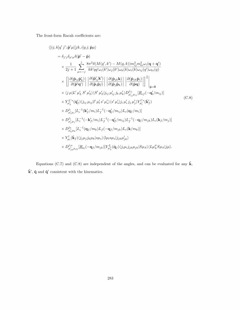
The front-form Racah coefficients are:

〈[ij, k]q′ j′; p′µ|[jk, i]q j; pµ〉

= δj′jδµ′µδ(p′ − p)

× 1

2j + 1

j∑

µ=−j

8π2δ(M(q′, k′) −M(q, k))m2ijm

2kiωi(q + q′)

kk′qq′ωi(k′)ωj(k′)ωk(k)ωi(k)ωij(q′)ωki(q)

×[∣∣∣∣∂(pijp

′k)

∂(p′q′)

∣∣∣∣∣∣∣∣∂(p′ijk

′)

∂(pipj)

∣∣∣∣∣∣∣∣∂(pjkk)

∂(pjpk)

∣∣∣∣∣∣∣∣∂(pjkpi)

∂(pq)

∣∣∣∣] 1

2

∣∣∣∣∣p=0

× 〈j µ|L′ µ′L S′ µ′S〉〈S′ µ′S |jij µ′ij jk µ′k〉Djij

µ′

ijµij

[Rcf (−q′t/mij)]

× Y L′∗µ′

L(q′f )〈jij µij |l′ µ′l s′ µ′s〉〈s′ µ′s|ji µ′i jj µ′j〉Y l′∗

µ′

l(k′f )

×Dji

µ′

iµi

[L−1c (k′f/mi)L

−1f (−q′f/mij)Lc(qf/mi)]

×Djj

µ′

jµj

[L−1c (−k′f/mi)L

−1f (−q′f/mij)L

−1f (−qf/mjk)Lc(kf/mj)]

×Djk

µ′

kµk

[L−1c (qf/mk)Lf (−qf/mjk)Lc(k/mk)]

× Y lµl

(kf )〈jjµjjkµk|sµs〉〈lµlsµs|jjkµ′jk〉

×Djjk

µ′

jkµjk

[Rtc(−qf/mjk)]Y Lµ′′

L(qf )〈jiµijjkµjk|SµS〉〈Lµ′′LSµS |jµ〉.

(C.8)

Equations (C.7) and (C.8) are independent of the angles, and can be evaluated for any k,

k′, q and q′ consistent with the kinematics.

283

APPENDIX D

Local Fields

The models presented in this review are relativistic quantum mechanical models but are not

local relativistic field theories. The goal of this section is to derive direct interaction models as

approximations to field theories. A connection to a field theory can provide constraints on model

interactions and consistent models of current operators.

To do this successfully we must devise a systematic procedure the that preserves Poincare

invariance, the quantum mechanical structure, the spectral condition, macroscopic locality, and

converges to the solution of the field theory in a precise sense. This goal is beyond the scope of

this paper. The discussion in this section will be limited to the first step, which is to formulate a

first approximation that leads to an instant form two-body model. It is important to note that

there is nothing special about the instant form. This could have been done equally as well in the

point or front-form.

In both relativistic and nonrelativistic quantum theories there are many types of “approxi-

mations” available. In many cases the approximation may look very different from a model with

a standard quantum mechanical interpretation. For instance, a standard optical potential, which

is used to reformulate elastic scattering, has an energy dependence due to eliminated degrees of

freedom which is not permitted in an ordinary Galilean invariant dynamics.

The models in this paper were designed to have most of the properties of a local relativistic

field theory. The only notable exception is property of microscopic locality which was replaced

by macroscopic locality. In formulating approximations it is desirable to preserve most of the

fundamental properties of the original theory. One type of approximation that retains most of

the properties of the original theory is an approximation where the exact Hamiltonian, H, is

replaced by a projected Hamiltonian, Hπ := ΠHΠ, for a suitable orthogonal projection operator

Π. This type of approximation will preserve conservation laws if the projectors commute with the

same operators that commute with the full Hamiltonian. The projection operators also preserve

the spectral condition. In order to interpret Hπ as an approximation to H we need an infinite

284

collection of projectors, Πn, that converge to the identity as n→ ∞ and a way of specifying how

the approximate models converge to the exact model.

We discuss approximation based on projection operators first for a model of a fixed number

of particles satisfying the constraints of Galilean relativity, then for a fixed number of particles

in a Poincare invariant theory, and finally for the case of a local field theory. This allows us

to separate the issues that relevant in treating scattering theory from those that are relevant to

Poincare invariance and those that are special to field theories.

D.1. Fixed Number of Particles - Galilean Invariance:

Consider a nonrelativistic quantum mechanical model of a system of N particles. The

dynamics of this system is governed by a Hamiltonian H, which in a Galilean invariant model

has the form P2/2M + h where h commutes with X, j, P, and M for the system (see (3.34)).

The Hilbert space for this system can be represented as the tensor product of the space of square

integrable functions of the total momentum with an internal Hilbert space, H:

H = L2(R2, d3P ) ⊗ H. (D.1)

Let Π be an orthogonal projection operator that commutes with X, J, P, and M . In general it

has the form

Π = I ⊗ Π (D.2)

where Π projects on a rotationally invariant subspace of the internal Hilbert space, H. For such

a projection operator define the projected Hamiltonian:

Hπ := ΠHΠ. (D.3)

If we define

K = MX (D.4)

then K, P, J, M , and Hπ satisfy the commutation relations for the central extension of the

Galilean Group. This defines a Galilean invariant approximate dynamics. To interpret this as

285

an approximation one has to specify a sequence Πn of projection operators on successively larger

subspaces such that Hn is well defined and converges to H. Since H has an unbounded energy

spectrum, the type of convergence needed is called strong resolvent convergence, which means

that

limn→∞

‖[(z −H)−1 − (z −Hn)−1]|Ψ〉‖ = 0 (D.5)

for all |Ψ〉 and z not an eigenvalue of H or Hn. This is a useful mathematical way of saying that

any bounded function of Hn strongly converges to the same bounded function of H.

When condition (D.5) holds we obtain a sequence of Galilean invariant approximations, Hπ,

P, J, K, M, to the exact dynamics, H, P, J, K, M. When the internal Hamiltonian, h,

has only discrete spectra, the eigenvalues of hn := ΠnhΠn become variational bounds on the

eigenvalues of h.

If the projection operators have finite dimensional range on the internal Hilbert space, H,

these approximate models will not allow scattering.

It is possible (Ch 80) to construct a sequence of projection operators Πn∞n=1 with infinite

dimensional range on the internal Hilbert space such that Hn is the Hamiltonian of a Galilean

invariant model that has a unitary scattering matrix, Sn, with the property that Sn weakly

converges to the exact scattering matrix as n → ∞. What is needed to be able to do this is

that Hn should cluster into a projector of a channel Hamiltonian onto an invariant subspace of

that channel Hamiltonian. The weak convergence of the approximate scattering operator requires

additional restrictions on the projection operators which can always be realized in applications.

The conclusion is that by choosing suitable sequences of projection operators, Πn∞n=1,

that converge strongly to the identity it is possible to construct a sequence of Galilean invariant

models that converge to the Galilean invariant dynamics in the following sense. The unitary rep-

resentations of the central extension of the Galilean group, Un(g), of the approximate dynamical

models converge strongly to the exact U(g) as n→ ∞ and the approximate scattering matrices,

Sn, converge weakly to the exact scattering matrix, S. The proof of the weak convergence of

286

the scattering operators can be found in (Ch 80) while the strong convergence of the group rep-

resentations follows from strong resolvent convergence of the approximate Hamiltonians on the

internal Hilbert space. Note that the strong convergence of the approximate unitary represen-

tations of the Galilean group implies nothing about the existence Sn or the convergence of the

Sn’s if they exist.

D.2. Fixed Number of Particles - Poincare Invariance:

Next we consider what happens to the framework discussed above if Galilean invariance is

replaced by Poincare invariance. In the Galilean invariant case it was possible to find a projection

operator that commuted with all of the generators of Galilean transformations except for the

Hamiltonian. This is impossible in the Poincare invariant case because the Hamiltonian appears

on the right hand side of some of the commutators. To see the problem compute the commutator

of Π with :

[Kj , P k]−

= −iδjkH. (D.6)

The Jacobi identity implies:

[Kj , [Π, P k]−]−

+ [P k, [Kj ,Π]−]−

= −iδjk[Π, H]−. (D.7)

The left hand side of (D.7) vanishes if Π commutes with all generators except H, while the right

hand side will not vanish under these conditions. This requires that if we want to preserve the

Poincare symmetry that several generators need to approximated simultaneously. The simplest

way to do this is to replace the generators with M and nine independent functions of the gen-

erators. We can always include generators of any kinematic subgroup in this collection of nine

operators, and this can be done independent of the existence of a true kinematic subgroup.

Thus, to construct the desired type of projections we let H, P, J, and K be the generators

of the system and construct both the Newton-Wigner position operator X and the mass operator

M . We introduce a sequence of Projection operators Πn that converge strongly to the identity

satisfying

287

Mn := ΠnMΠn →M (D.8)

in the sense of strong resolvent convergence and

[Πn,P]−

= [Πn,J]−

= [Πn,X]−

= 0. (D.9)

For this sequence of projection operators the operators P, J,

Hπ =√M2

π + P2 (D.10)

and

Kπ = −1

2Hπ,X+ − 1

Hπ +Mπ(P× j). (D.11)

where j = J−X×P satisfy the commutation relations for the Poincare Lie algebra. At this point,

the analysis reduces to that of the non-relativistic case. The only complication is constructing a

suitable set of projection operators that permit scattering and commute with X. This difficulty

is that X can be a complicated dynamical operator that may depend on interactions.

One way to avoid these complications is to construct a sequence of Euclidean invariant

projectors satisfying:

[X,Π]−6= 0. (D.12)

This leads to a alternative sequence of approximations which are suitable, but not as elegant.

First we note, since the projectors commute with the Euclidean group, the model mass operator

remains Euclidean invariant with respect to the full dynamics. This means that it has the

following representation:

〈P′ · · · |Mπ|P · · ·〉 =

δ(P′ − P)〈(· · ·)′‖Mπ(P)‖ · · ·〉 (D.13)

where the reduced mass operator, Mπ(P), is rotationally invariant.

288

In the case that X commutes with Π the Mπ(P)’s for different values of P are scattering

equivalent. This is a consequence of the Poincare invariance of the approximate scattering ma-

trices. The construction of the unitary operator that makes the equivalence is outlined below.

The Poincare invariance of the scattering matrix implies

〈P′ · · · |S|P · · ·〉 = δ(P′ − P)〈(· · ·)′‖S‖ · · ·〉 (D.14)

with S independent of P. Using this we have

S = Ω†+(P)Ω−(P) = Ω†+(P′)Ω−(P′). (D.15)

Asymptotic completeness can be used to write this as

B(P′;P) = |b(P′)〉〈b(P)|+ Ω−(P)Ω†−(P) = |b(P′)〉〈b(P)| + Ω+(P′)Ω†+(P) (D.16)

where |b(P)〉 are the point eigenstates of M(P) which may in principle depend on P. The

Euclidean invariance and intertwining properties of the wave operators can then be used to show

that B(P′;P) is maps M(P) to M(P′) . Equation (D.16) shows that map preserves the scattering

operator. The multichannel generalization of the above construction can be found in (Co 82).

If instead we assume (D.12) then the Mπ(P)’s for different values of P are not equivalent.

The reason for this is that the projection breaks the Poincare invariance of the full theory as

was illustrated in (D.7). These approximations still preserve the Euclidean invariance of the full

theory.

It is possible to restore Poincare invariance by changing the model mass operator, Mπ → Mπ,

to

289

〈P′ · · · |Mπ|P · · ·〉 :=

δ(P′ − P)〈(· · ·)′‖Mπ(0)‖ · · ·〉. (D.17)

It follows the if we take Xπ = i∇p, and define

Hπ =√M2

π + P2 (D.18)

and

Kπ = −1

2Hπ,Xπ+ − 1

Hπ + Mπ(p × jπ). (D.19)

where jπ = J − Xπ × P, then Hπ, Kπ, P, J satisfy the Poincare commutation relations. They

can be used to construct a unitary representation, Uπ(Λ, a), of the Poincare group corresponding

to these approximate generators.

In this case, as the projection operators converge to the identity, the operators Mπ no longer

converge to M ; instead we expect that if the exact mass operator has the representation

〈P′, · · · |M |P, · · ·〉 =

δ(P′ − P)〈(· · ·)′‖M(P)‖ · · ·〉. (D.20)

the projected operators will converge to an operator M with kernel

〈P′, · · · |Mn|P, · · ·〉 → 〈P′, · · · |M |P, · · ·〉 =

δ(P′ − P)〈(· · ·)′‖M(0)‖ · · ·〉. (D.21)

If the exact model has an asymptotically complete, Poincare invariant scattering operator then

the right hand side of (D.21) is related to the right hand side of (D.20) by a scattering equivalent

unitary transformation of the form (D.16) :

290

BMB† = M (D.22)

where

〈P′, · · · |B|P, · · ·〉 =

δ(P′ − P)〈(· · ·)′‖B(P;0)‖ · · ·〉. (D.23)

Thus in this case we expect that with a suitable set of projectors that

Un(Λ, a) → B†U(Λ, a)B (D.24)

and

Sn → S = S (D.25)

where the convergence in (D.24) will be strong and the convergence in (D.25) will be weak. In

the relativistic case neither of these statements have been proved, but they are suggested by the

non-relativistic results.

It is worth noting that in this example the approximations were purely Bakamjian-Thomas

models which we argued in section 6 violated cluster properties. We learned restore macroscopic

locality with packing operators in section 7. If we let

Un(Λ, a) = AnUn(Λ, a)A†n (D.26)

where An are packing operators in the model system, then we expect that these macrolocal

approximations will converge to

Un(Λ, a) → AB†U(Λ, a)BA† (D.27)

where A = limAn. If all of the limits exist and behave as expected then AB† is a Euclidean

invariant unitary operator that preserves the scattering operator and cluster properties. It is

291

simply a change of representation that preserves all of the physics. In this case the convergence

of the scattering matrix is not affected.

D.3. Fields

We are now ready to generalize what was discussed above for fixed N to the case of a local

field theory. To keep the discussion as simple as possible consider the construction of an instant

form two-body model based on a local relativistic field theory with a single Hermitian scalar field

φ(x) of mass m > 0. Our discussion will be limited to the construction of a projection operator on

a “two-body” subspace of the field theory on which a model scattering theory can be formulated.

One projection operator does not by itself define an approximation. To complete the task

started here and construct a convergent set of projectors that allow scattering is a research

problem. The justification for this first step should be understood in the context of the previous

section. Our limited goal in this section is to construct the analog of Mπ in the case of a field

theory. The main problem involves identifying a one particle subspace of the physical Hilbert

space, and using the operators that create the one particle subspace to construct a subspace that

behaves enough like a two particle subspace to allow scattering.

It is clear that one could treat this problem using combinations of perturbative and Fock

space methods. This does not provide a justification of these models in the context of quantum

field theory, but instead only in the limited scope of perturbative field theory. Because of this we

discuss the formulation of approximations in a manner that does not require perturbation theory.

Having said this we need some assumptions to start our construction. To this end we assume

1. The field φ(x) satisfies the Wightman axioms for a Hermitian scalar field of mass m > 0.

2. The physical Hilbert space has a Poincare invariant one particle subspace Hm corresponding

to a particle of mass m and spin 0. The Poincare group acts irreducibly on this subspace.

3. The field has non-vanishing matrix elements between the vacuum and the one particle sub-

space, Hm.

4. The two point function of this field has a Lehmann representation of the form

292

〈0|φ(x)φ(y)|0〉 =

−iD−m(x− y) − i

∞∫

4m2

D−√λ(x− y)dµ(λ). (D.28)

Equation (D.28) implies a normalization of the field.

The first assumption defines properties of the field in the absence of a perturbative descrip-

tion. The second assumption implies that this model admits particles of mass m the behave

in the expected way and assumes that there is only one type particle with mass m. The third

assumption ensures the existence of a Lehmann representation for the two-point function. The

fourth assumption is about the structure of this Lehmann representation; what is says is that on

the subspace spanned by vectors of the form

φ(f)|0〉 =

∫f(x)φ(x)|0〉d4x (D.29)

that the one and many-body parts of this subspace can be easily isolated.

We show how to use the Heisenberg fields to construct 2-body projection operators that allow

one construct models of a finite number of degrees of freedom that permit scattering. The model

constructed corresponds to the dynamics generated by Uπ(Λ, a) in the previous section. Our

development is limited to the two-body problem. The elements of this construction summarized

below:

1. Construct a unitary mapping, Φ1, from an irreducible representation space H1 of the Poincare

group with the same mass and spin as the particle to the invariant one particle subspace of

the field theory, Hm, that satisfies the intertwining relation:

Φ1U1(Λ, a) = U(Λ, a)Φ1 (D.30)

where U1(Λ, a) is the irreducible representation of the Poincare group on H1 and U(Λ, a) it

293

the physical representation of the Poincare group associated with the field theory. This is

done using Hagg’s (Ha 58) notion of a quasilocal field.

2. Construct a unitary mapping Φ2 from the symmetric subspace of H2 := H1 ⊗ H1 to a

subspace of the physical Hilbert space that satisfies the intertwining relation for the Euclidean

subgroup:

Φ2U1(R, a) ⊗ U1(R, a) = U(R, a)Φ2 (D.31)

3. Construct a model two-body mass operator M2 using the approximation (D.21) in M2 =

Φ†2MΦ2.

This leads to a Bakamjian Thomas model with a mass operator determined entirely by the

field.

D.4. Quasilocal Fields

The first step in the construction is to identify the physical one particle subspace of the field

theory. In general if a smeared Heisenberg field is applied to the vacuum the resulting vector will

have both one and many particle components. The second term in the Lehmann representation

(D.28) comes from these many-body components. One way to ensure that the result of applying

the smeared Heisenberg field to the vacuum lies in the physical one-particle subspace of the field

theory is to smear the field with a function whose fourier transform is a function of the four

momentum that is identically zero when p2 is in the continuous (mass)2 spectrum of the field

theory and 1 when p2 = −m2. It will be shown, using the assumption about the Lehmann

representation, that if such a smeared field is applied to the vacuum that the resulting vector is

in the one particle Hilbert space of the field theory. The full one particle subspace is the closed

linear subspace containing this vector and finite linear combinations of vectors related to this by

Poincare transformations. By assumption this subspace carries an irreducible representation of

the Poincare group.

294

To formalize this procedure, following Haag (Ha 58), introduce the notion of a quasilocal

covariant field. To construct this field let h(p) be a smooth function of p2 with the following

properties:

h(p) =

1 if p2 = −m2;

0 if |p2 +m2| > 2m2. (D.32)

This means that it is a smooth function of p2 that is identically 1 on the point mass spectrum

and identically 0 in a neighborhood of the continuous spectrum. Denote the fourier transform of

the field φ(x) by

φ(p) := (2π)−2

∫d4xe−ip·xφ(x) (D.33)

and define the following quasilocal field operator

A(p) := h(p)φ(p). (D.34)

The reason for doing this is that the energy spectrum of the one particle states and many particle

states are not disjoint, although the mass spectrum is. The function h(p) separates these two

independent parts of the dynamics. It will be shown that if a smeared quasilocal field of this form

is applied to the vacuum the resulting vector is an element of the physical one particle subspace

of the Hilbert space. The fourier transform of A(p) is denoted by A(x):

A(x) := (2π)−2

∫d4peip·xA(p). (D.35)

which also has the form

A(x) = (2π)−2

∫d4yh(x− y)φ(y). (D.36)

where

295

h(x) = (2π)−2

∫d4peip·xh(p). (D.37)

The operator A(x) has many of the properties of a field operator φ(x). These follow form the

definitions and the axioms satisfied by the Heisenberg fields. These will be stated without proof.

It transforms covariantly under the action of Poincare transformations:

U(Λ, a)A(x)U †(Λ, a) = A(Λx+ a) (D.38)

or equivalently

U(Λ, a)A(p)U †(Λ, a) = eiΛp·aA(Λp). (D.39)

The infinitesimal generators of U(Λ, a) can be computed on vectors constructed from polynomials

in the quasilocal fields applied to the vacuum using equations (D.38) or (D.39):

PµA(x1) · · ·A(xn)|0〉 =

−in∑

k=1

A(x1) · · ·∂

∂xkµA(xk) · · ·A(xn)|0〉 (D.40)

JµνA(x1) · · ·A(xn)|0〉 =

−in∑

k=1

A(x1) · · ·(xµ

k

∂

∂xkν− xν

k

∂

∂xkµ

)A(xk) · · ·A(xn)|0〉 (D.41)

or equivalently

PµA(p1) · · · A(pn)|0〉 =

( n∑

k=1

pµk

)A(p1) · · · A(pn)|0〉 (D.42)

296

JµνA(p1) · · · A(pn)|0〉 =

−in∑

k=1

A(p1) · · ·(pµ

k

∂

∂pkν− pν

k

∂

∂pkµ

)A(pk) · · · A(pn)|0〉. (D.43)

The mass operator can be computed from (D.42):

MA(p1) · · · A(pn)|0〉 =

(−

n∑

k=1

p2k

)1/2A(p1) · · · A(pn)|0〉 (D.44)

It also satisfies the same cluster properties as the Heisenberg field:

lim|a−b|→∞

〈0|A(x+ a)A(y + b)A(z + a)A(w + b)|0〉−

〈0|A(x)A(z)|0〉〈0|A(y)A(w)|0〉

= 0 (D.45)

etc. For the case of quasilocal fields this equation holds both if the fields are smeared over

test functions of the space or spacetime variables. For the Heisenberg field it must generally be

smeared over test functions of the spacetime coordinated for this to be true.

The operator A(x) has two properties that are characteristic of free fields that are not shared

by the Heisenberg field φ(x). First it has the same two point function as a free field operator:

〈0|A(x)A(y)|0〉 = −iD−m(x− y). (D.46)

where

−iD−m(x) =

(2π)−3

∫e−ik·xθ(−k0)δ(k2 +m2)d4k =

(2π)−3

∫eik·xθ(k0)δ(k2 +m2)d4k (D.47)

is the two-point Wightman function for a free field. Second it has the property that the “sharp

297

time” fields smeared over test functions of x are well defined operators:

a†(x) := A(x, 0) (D.48)

a†(p) = (2π)−3/2

∫d3xe−ip·xa†(x) (D.49)

a†(f) :=

∫d3xf(x)a†(x) :=

∫d3pf(p)a(p). (D.50)

In general the Heisenberg field must be smeared over test functions of both space and time before

it becomes an operator. Thus, one of the fundamental advantages of the quasilocal fields is that

is possible to restrict the field to a suitable three-dimensional surface, as in (D.48). We will

see that the choice of t = 0 implies that the Euclidean subgroup of the model is exactly the

Euclidean subgroup of the field. What is given up is that these quasi-local fields do not satisfy

local commutation relations.

D.5. The One-Body Subspace

We now show that a†(f)|0〉 is an element of the one particle subspace of the field theory and

that a†(p)|0〉 is a simultaneous eigenstate of the four momentum of the field theory.

To show that a†(f) is an element of the one particle subspace we must show that is an

eigenstate of the mass operator with eigenvalue m2. To show this is to compute the expectation

value of M2 and its dispersion in the state a(f)|0〉. This can be done analytically using (D.31),

(D.33), (D.43), (D.45), (D.46), and (D.49) with the result:

〈M2〉 = m2 〈M4〉 = m4 (D.51)

from which we conclude

〈(〈M2〉 −M2)2〉 = 0. (D.52)

Since there is no dispersion we conclude that a(f)|0〉 is an eigenstate of M 2 with eigenvalue m2.

By the spectral condition the mass operator of the field theory is non-negative and must be equal

298

to the unique (Re 72) non-negative square root of M 2. It follows that a†(f)|0〉 is an eigenstate

of the mass operator with eigenvalue m and necessarily an element of the one particle subspace

of the field theory.

By direct computation using (D.42) we find

P a†(p)|0〉 = p a†(p)|0〉 (D.53)

which shows that a†(p)|0〉 is a generalized eigenstate of the linear momentum operator with

eigenvalue p.

The irreducible representation space for a spinless particle of mass m is spanned by the

simultaneous eigenstates of the three momentum. Thus we conclude that the vectors a†(f)|0〉

are dense in the single particle subspace of the physical Hilbert space.

Note although a†(p) looks like an ordinary creation operator, we have made no assumptions

about the commutation relations. In general the eigenstates need to be renormalized. Although

in the one-body case the renormalization is trivial, it is useful to cast the renormalization in a

general form that can also be applied to the two-body case.

To renormalize these states let f(p) be a square integrable function of the three momentum

with normalization:

∫d3p|f(p)|2 = 1. (D.54)

We denote the Hilbert space of functions with the norm (D.54) by H1. Let Φ1 denote the

mapping from H1 to the one particle subspace of the Hilbert space defined by

Φ1(f) := a(f)|0〉. (D.55)

The operator Φ1 clearly maps the momentum operator on H1 to the restriction of the momentum

operator of the field theory to the one particle subspace of the field theory. This operator is not

299

a unitary mapping form H1 to Hm. To renormalize the vectors on Hm we replace Φ1 by an

operator that

i. has the same range as Φ1,

ii. preserves the three momentum, and

iii. preserves the H1 norm of f .

Such an operator is given by

Φ1 := Z−1/2Φ1 (D.56)

where Z is a wave function renormalization operator given by

Z−1 = (Φ1Φ†1)−1mp (D.57)

Note that in general Φ1Φ†1 does not have an inverse on the full physical Hilbert space, but there

is a well defined inverse on the range of Φ1 called the Moore-Penrose generalized inverse. The

quantity (Φ1Φ†1)−1/2mp is the Moore Penrose generalized inverse of the square root of Φ1Φ

†1. The

Moore Penrose generalized inverse X−1mp of a linear operator X is the unique solution to the four

Penrose equations (Na 76):

X−1mpXX

−1mp = X−1

mp (D.58)

XX−1mpX = X (D.59)

XX−1mp = ΠR(X)

(D.60)

300

X−1mpX = ΠN (X)⊥ (D.61)

where ΠR(X)and ΠN (X)⊥ are orthogonal projectors on the closure of the range of X and the

orthogonal complement of the null space of X respectively.

In this particular case the range of both projection operators is the one particle subspace of

the field theory. Although there are convergent iterative algorithms for computing the Moore-

Penrose generalized inverse of an operator, in this case the unique solution of the 4-Penrose

equations can be written down explicitly. From the definitions:

Z = Φ1Φ†1 =

∫d3pa†(p)|0〉d3p〈0|a(p) (D.62)

and by direct computation:

(Φ1Φ†1)

1/2 =

∫d3pa†(p)|0〉d3p

(2ωm(p)

)1/2〈0|a(p) (D.63)

From these expressions it follows that

(Φ1Φ†1)−1/2mp =

∫d3pa†(p)|0〉d3p

(2ωm(p)

)3/2〈0|a(p) (D.64)

satisfies the 4 Penrose equations.

The renormalized injection operator Φ1 is

Φ1(p) :=(2ωm(p)

)1/2Φ1(p) =

(2ωm(p)

)1/2a†(p)|0〉 = a†r(p)|0〉. (D.65)

Thus we see that in this special case the wave function renormalization factor is Z−1/2 =(2ωm(p)

)1/2This result could have been obtained by directly computing 〈0|a†(p)a(p′)|0〉 and

including the factors so it has the normalization, δ3(p − p′), consistent with (D.54). The renor-

malization procedure defined by (D.56) and (D.57) has the virtue that is generalizes without

change to the two-body case.

301

The renormalized injection operator Φ1 is a unitary operator form H1 to Hm. To see this

note that the Penrose equations imply:

Φ1Φ†1 = (Φ1Φ

†1)−1/2mp (Φ1Φ

†1)(Φ1Φ

†1)−1/2mp (D.66)

is the orthogonal projector on the one particle subspace of the physical Hilbert space and

Φ†1Φ1 = Φ†1(Φ1Φ†1)−1mp Φ1 (D.67)

which is the identity on H1. This follows because H1 is the range of Φ†1, so any vector in H1 can

be expressed in the form Φ†(X) for some X in the one particle subspace of the Hilbert space.

By unitarity of Φ1 it follows that

U1(Λ, a) := Φ†1U(Λ, a)Φ1 (D.68)

is an irreducible unitary representation of the Poincare group on H1. Because Φ intertwines with

the momentum, (i.e. the momentum in H1 has the same value as the momentum of the particle

in the field theory), it follows from the unitarity that this representation necessarily has the form

(U1(Λ, a)f

)(p) = e−i(ωm(p)a0−p·a)f(p′)

√ωm(p′)ωm(p)

(D.69)

where

p′ := Λ−1(ωm(p),p). (D.70)

302

D.6. The Two-Body Subspace

Unlike the one particle sector of the physical Hilbert space of a local field theory, there is

no Poincare invariant two particle subspace of the physical Hilbert space (except in a free field

theory). What we need is a subspace that allows us to construct a suitable two-body scattering

theory. A minimal requirement for a two body scattering theory is that when the two “particles”

are separated by asymptotic spacelike distances that the Hamiltonian becomes a sum of single

particle Hamiltonians.

To begin this construction we define our “two-body” subspace by applying the operators used

to construct the one particle space twice to the vacuum. Formally we construct the mapping Φ2

from

H2 := H1 ⊗H1 (D.71)

to the physical Hilbert space. Define the mapping Φ2 :

Φ2(f1, f2) :=1

2

(a†r(f1)a

†r(f2) + a†r(f1)a

†r(f2)

)|0〉. (D.72)

Note that the renormalization factors can be absorbed into the definitions of the functions f1

and f2 using:

fir(p) :=√

2ωm(p)fi(p) (D.73)

which implies

a†f (f) =

∫d3xfr(x)A(x, 0). (D.74)

Using this we can show that Φ2 intertwines the Euclidean group and satisfies cluster properties.

To show the Euclidean invariance first note:

303

U(R, a)Φ2(f, g) =

1

2

∫d3xd3y

(gr(x)fr(y) + gr(y)fr(x)

)×

A(Rx + a, 0)A(Ry + a, 0)|0〉 =

1

2

∫d3xd3y

[gr(R

−1(x− a))fr(R−1(y − a)) + gr(R

−1(y − a))fr(R−1(x− a))

]×

A(x, 0)A(y, 0)|0〉. (D.75)

Since the renormalized functions f and g involve multiplication of the original functions in mo-

mentum space by a rotationally invariant function, the configuration space functions are the

convolution of the unrenormalized configurations space function with a rotationally invariant

distribution. This means that the renormalization is Euclidean invariant - or equivalently Eu-

clidean transformations and renormalizations can be done in any order. It follows that the Eu-

clidean transformed renormalized functions in (D.75) can be replaced by renormalized Euclidean

transformed functions:

fr → fr (R,a)(x) = fr(R−1(x− a)) (D.76)

gr → gr (R,a)(x) = gr(R−1(x− a)). (D.77)

This can be summarized concisely by the following equation:

304

U(R, a)Φ2 = Φ2U(R, a) ⊗ U(R, a) (D.78)

which shows that Φ2 intertwines the physical representation of the Euclidean subgroup with the

tensor product representation of H2.

To show that Φ2 has the desired cluster properties consider

lim|a−b|→∞

Φ†2(f(I,a), g(I,g))HΦ2(f(I,a), g(I,g))H =

lim|a−b|→∞

∫d3xd3yd3x′d3y′×

1

4f∗r (x)g∗r(y))fr(x

′)gr(y′)×

〈0|A(x + a, 0)A(y + b, 0) +A(y + b, 0)A(x + a, 0)H×

A(x′ + a, 0)A(y′ + b, 0) +A(y′ + b, 0)A(x′ + a, 0)|0〉. (D.79)

Using cluster properties of the quasilocal fields, (D.45) translational invariance of the vacuum,

and the expression for H in (D.42) this becomes:

∫d3xd3yd3x′d3y′×

f∗r (x)g∗r (y))fr(x′)gr(y

′)×

305

〈0|A(x, 0)HA(x′, 0)|0〉〈0|A(y, 0)A(y′, 0)|0〉+

〈0|A(x, 0)A(x′, 0)|0〉〈0|A(y, 0)HA(y′, 0)|0〉 =

Φ†1(f)HΦ1(f)Φ†1(g)Φ1(g) + Φ†1(f)Φ1(f)Φ†1(g)HΦ1(g). (D.80)

This is the sum of the one-body Hamiltonians. In momentum space the right hand side of (D.80)

has the familiar form:

→ δ(p1 − p′1)δ(p2 − p′2)(ωm(p1) + ωm(p2)

). (D.81)

In general, the operator Φ2, is not a-priori a unitary mapping from the symmetric subspace of

H2 to a Euclidean invariant subspace of the field theory. This can be fixed with one more wave

function renormalization. The renormalization can be treated as in the one-body case. Define

the renormalized injection operator:

Φ2 := Z−1/22 Φ2 (D.82)

where

Z−12 = (Φ2Φ

†2)−1mp (D.83)

It follows from the Penrose equations that Φ2Φ†2 and Φ†2Φ2 are orthogonal projection operators.

The first of these operators is the projection on the range of Φ2, which is a Euclidean invariant

subspace of the field theory, while the second of these is the orthogonal projector on the symmetric

subspace of H2. It follows that Φ2 is a unitary mapping between these subspaces.

306

Because Φ2 intertwines with the Euclidean group it follows that Z2 is Euclidean invariant

and consequently that Φ2 also intertwines with the Euclidean group.

To show that the renormalization does not interfere with cluster properties note first that

(Φ2Φ†2)−1/2mp Φ2 = Φ2(Φ

†2Φ2)

−1/2mp (D.84)

Next consider Φ†2Φ2, which is a mapping on H2. Up to one-body renormalizations factors it is

the 4-point function of the quasilocal field A with each factor restricted to time 0. The operator

Φ†2Φ2 can be expanded in its truncated parts, using the property that 〈0|A(x)|0〉 = 0 because the

range of A is in the one particle subspace which is orthogonal to the vacuum. By examining the

properties of each of the truncated pieces with the one-body renormalization factors included it

can be shown to have the asymptotic form

Φ†2Φ2 → 1

2ΠH2symmetric

(D.85)

where ΠH2symmetricis the projector on the symmetric subspace of H2. This means that up to

normalization it asymptotically becomes the identity when the particles are separated. Similarly

(Φ†2Φ2)−1/2mp is asymptotically a different constant multiple of the identity. The unitarity ensures

that if we evaluate the expectation value of the energy in a completely symmetric wave function

corresponding to two asymptotically separated particles that the expectation value will be ap-

proximately the sum of the expectation values of the energies of each particle. What this means

is that on the symmetric subspace of H2 that

Φ†2HΦ2 = ωm(p1) + ωm(p2) + V2 (D.86)

where the interaction V2 is short ranged, Euclidean invariant, and has the form

307

〈p′′1 p′′2 |V |p′1 p′2〉 =

Φ†2(p′′1 p′′2)(P 0 − ωm(p1) − ωm(p2))Φ

†2(p′1 p′2) =

δ(P′′ − P′)〈p′′1 p′′2‖V2(0)‖p′1 p′2〉 (D.87)

where P = p1 + p2 is the total momentum. For the reasons discussed previously, the interaction

for different values of P do not define scattering equivalent models.

A relativistic dynamics is obtained by replacing the interaction defined above by:

〈p′1 p′2|V2|p1 p2〉 =

δ(P′ − P)〈k′1 − k′1‖V2(0)‖k1 − k1〉 (D.88)

which involves factoring out the momentum conserving delta function and replacing the remaining

momenta by ki = L−1c (P )pi evaluated on the one-particle mass shell. The operators

Mπ = 2ωm(k) + V2 (D.89)

X = i∇p (D.90)

P := Φ†2PΦ2 (D.91)

308

J := Φ†2JΦ2, (D.92)

where the first two expressions are representation dependent; they can be used to construct a

Bakamjian-Thomas dynamics. To define the model dynamics let

H =√M2 + P2 (D.93)

and

K = −1

2H,X+ − 1

H + M(P× j). (D.94)

where j = J − X × P. It follows that H, K, P, J satisfy the Poincare commutation relations.

They can be used to construct a model dynamics following the construction of section 5.

It is useful to write the desired model interaction directly in terms of the renormalized fields,

φr(x) := Z−1/21 φ(x), and the two-body renormalization operators:

〈p′′1 p′′2 |V2|p′1 p′2〉 =

1

(2π)2

∫dp′′01 dp′′02 dp′01 dp

′02 h(p

′′1)h(p′′2)h(p′1)h(p

′2)〈0|φr(p

′′2)φr(p

′′1)(Z

−1/22 )†×

(P 0 − ωm(p1) − ωm(p1)

)(Z−1/22 )φr(p

′1)φr(p

′2)|0〉. (D.95)

This formula gives the interaction (D.87) which must be restricted as in (D.88) to obtain the

interaction V2. This construction applies to the two-body system. It gives explicit formulas for

the interactions in terms of field theoretic quantities. These interactions can depend on the

functions h(x) used to define the quasilocal fields.

An analogous construction can be used to construct two-body current matrix elements:

309

〈p′′1 p′′2 |Iµ(x)|p′1 p′2〉 =

1

(2π)2

∫dp′′01 dp′′02 dp′01 dp

′02 h(p

′′1)h(p′′2)h(p′1)h(p

′2)〈0|φr(p

′′2)φr(p

′′1)(Z

−1/22 )†×

Iµ(x)(Z−1/22 )φr(p

′1)φr(p

′2)|0〉. (D.96)

or matrix elements of any field combination of field operators. In this case because the projection

operators are Euclidean invariant this projected current operator will satisfy Euclidean covari-

ance, but will not generally be Lorentz covariant or satisfy current conservation. This can be

restored, in a manner similar to the way in which Poincare invariance was restored, by comput-

ing dynamically independent current matrix elements and using current covariance and current

conservation to determine the remaining matrix elements. These computations should be done

using wave functions associated with the barred representation. Similar remarks apply to any

Lorentz tensor operators.

The construction in this section can be modified to treat forms of the dynamics other than

the instant form. In principle one should be able to extend this to treat more complex systems,

although in these cases other consideration such as cluster properties become relevant. The

general principle is that as one systematically increases the range of the injections operators

one should expect that the model can be systematically improved. The extension to system

of confined quarks can be treated with some modifications of the starting assumptions. For

nucleons, the quasilocal fields must be constructed out of three quark fields coupled to a color

singlet. This combination of fields must have non-vanishing matrix elements between the vacuum

and one particle (i.e. hadron) states. In this case there will be constraints on the structure of

the six-point function as well as the two-point and four point functions.

310

An 32 C. D. Anderson, Phys. Rev. 41, 405 (1932).

Ba 47 V. Bargmann, Ann. Math. 48, 568 (1947).

Ba 48 V. Bargmann and E. P. Wigner, Proc. Nat. Acad. 34, 211 (1948).

Ba 53 B. Bakamjian and L. H. Thomas, Phys. Rev. 92, 1300 (1953).

Ba 54 V. Bargmann, Ann. Math. 59, 1 (1954).

Ba 79 B. L. G. Bakker, L. A. Kondratyuk and M. V. Terent’ev, Nucl. Phys. B158, 497 (1979).

Be 47 H. A. Bethe, Phys. Rev. 72, 339 (1947).

Be 76 V. B. Berestetskii and M. V. Terent’ev, Yad. Fiz. 24, 1044 (1976) [Sov. J. Nucl.

Phys. 24, 547 (1976)].

Be 77 V. B. Berestetskii and M. V. Terent’ev, Yad. Fiz. 25, 653 (1977) [Sov. J. Nucl. Phys. 25,

347 (1977)].

Be 80 M. Betz and F. Coester, Phys. Rev. C21, 2205 (1980).

Be 81 M. Betz and T.-S.H. Lee, Phys. Rev. C23, 375 (1981).

Be 82 V. B. Berestetski, E. M. Lifshitz and L. P. Pitaevskii, Quantum Electrodynamics, 2nd

Ed. (Oxford: Pergamon, 1982).

Be 85 E. Berger and F. Coester, Phys. Rev. D32, 1071 (1985).

Be 87 E. Berger and F. Coester, Ann. Rev. Nuc. Part. Sci. 37,463 (1987).

Bi 62 M. Birman, Dokl. Akad. Nauk USSR. 143, 506 (1962).

Bj 64 J. D. Bjorken and S. D. Drell, Relativistic Quantum Mechanics (New York: McGraw-

Hill, 1964).

Bj 66 J. D. Bjorken, Phys. Rev. 148, 1467 (1966).

Bl 52 J. M. Blatt and V. F. Weisskopf, Theoretical Nuclear Physics (New York: Wiley, 1952),

Chapter XII.

Bl 60 R. Blankenbecler and L. F. Cook, Phys. Rev. 119, 1745 (1960).

Bl 66 R. Blankenbecler and R. Sugar, Phys. Rev. 142, 1051 (1966).

311

Bo 35 M. Born, W. Heisenberg and P. Jordan, Z. Phys. 35, 557 (1926).

Bo 59 N. N. Bogoliubov and D. V. Shirkov, Introduction to the Theory of Quantized Fields,

(New York: Wiley-Interscience, 1959), pp. 147-153.

Br 59 W. Brenig and R. Haag, Fortsch. Phys. 7, 183 (1959); [translation in Quantum Scat-

tering Theory, Ed. M. Ross (Bloomington, IN: Indiana University Press, 1963), p. 13.]

Ca 83a J. Carlson, J. B. Kogut and V. R. Pandharipande, Phys. Rev. D27, 233 (1983).

Ca 83b J. Carlson, J. B. Kogut and V. R. Pandharipande, Phys. Rev. 28, 2807 (1983).

Ca 90 Z.-J. Cao and B. D. Keister,, Phys. Rev. C42, 2295 (1990).

Ch 73 S.-J. Chang, R. G. Root, and T.-M. Yan, Phys. Rev. D7, 1133 (1973).

Ch 76 C. Chandler and A. Gibson, Indiana J. Math. 25, 443 (1976).

Ch 79 M. Chemtob, in Mesons in Nuclei, Ed. M. Rho and D. H. Wilkinson (Amsterdam:

North-Holland, 1979), p. 495.

Ch 86 P.-L. Chung and W. N. Polyzou, Book of Contributions, Eleventh International IUPAP

Conference on Few-Body Systems in Particle and Nuclear Physics, Ed. T. Sasakawa et

al. (Supplement to Research Report of Laboratory of Nuclear Science, Tohoku Univer-

sity, Vol. 19, 1986), p. 102.

Ch 88a P.-L. Chung, F. Coester, B. D. Keister and W. N. Polyzou, Phys. Rev. C37, 2000

(1988).

Ch 88b P.-L. Chung, F. Coester and W. N. Polyzou, Phys. Lett. B205, 545 (1988).

Ch 89 P.-L. Chung, B. D. Keister and F. Coester, Phys. Rev. C39, 1544 (1989).

Cl 70 F. Close and H. Osborn, Phys. Rev. D2, 2127 (1970).

Cl 71 F. Close and H. Osborn, Phys. Lett. B34, 400 (1971).

Co 57 J. Cook, J. Math. Phys. 36, 82 (1957).

Co 65 F. Coester, Helv. Phys. Acta 38, 7 (1965).

Co 75 F. Coester and A. Ostebee, Phys. Rev. C11, 1836 (1975).

312

Co 82 F. Coester and W. N. Polyzou, Phys. Rev. D26, 1348 (1982).

Co 87 F. Coester in Constraint Theory and Relativistic Dynamics, Ed. G. Longhi and L.

Lusanna (Singapore: World Scientific, 1987).

Co 88 F. Coester inProceedings of the International Spring School on Medium- and High-

Energy Nuclear Physics, (Taipei, Taiwan, 1988).

Cu 63a D. G. Currie, T. F. Jordan and E. C. G. Sudarshan, Rev. Mod. Phys. 35, 350 (1963).

Cu 63b D. G. Currie, J. Math. Phys. 4, 1470 (1963).

De 66 T. DeForest, Jr. and J. D. Walecka, Adv. Phys. 15, 1 (1966).

De 79 L. Delker, et al., Phys. Rev. Lett. 42, 89 (1979).

Di 27 P. A. M. Dirac, Proc. R. Soc. London A114, 243 (1927).

Di 28 P. A. M. Dirac, Proc. R. Soc. London A117, 610 (1928).

Di 30 P. A. M. Dirac, Proc. Cam. Phil. Soc. 26, 376 (1930).

Di 49 P. A. M. Dirac, Rev. Mod. Phys. 21, 392 (1949).

Di 50 P. A. M. Dirac, Can. J. Math., 2, 129 (1950).

Do 26 T. deDonder and H. van Dungen, Compt. Rend., July 1926.

Do 79 B. de Dormale, J. Math. Phys. 20, 1229 (1979).

Dr 64 S. D. Drell and J. D. Walecka, Ann. Phys. 28, 18 (1964).

Du 83 B. Durand and L. Durand, Jr., Phys. Rev. D28, 932 (1983) .

Dy 52 F. J. Dyson, Phys. Rev. 85, 5 (1952).

Dz 88a Z. Dziembowski, Phys. Rev. D37, 768 (1988).

Dz 88b Z. Dziembowski, Phys. Rev. D37, 778 (1988).

Fa 65 L. D. Faddeev, Mathematical Aspects of the Three-Body Problem in the Quantum

Scattering Theory (Jerusalem: Israel Program for Scientific Translation, 1965).

Fo 26a V. Fock, Z. Phys. 38, 242 (1926).

313

Fo 26b V. Fock, Z. Phys. 39, 226 (1926).

Fo 48 H. M. Foley and P. Kusch, Phys. Rev. 73, 412 (1948).

Fo 61 L. Foldy, Phys. Rev. 122, 275 (1961).

Fo 64 R. Fong and J. Sucher, J. Math. Phys. 5, 456 (1964).

Fo 74 L. Foldy and R. Krajcik, Phys. Rev. Lett. 32, 1025 (1974).

Fr 73 J. L. Friar, Ann. Phys. 81, 332 (1973).

Fr 74 J. Frohlich, Ann. Inst. H. Poincare A21, 271 (1974).

Fr 76 J. L. Friar, Nucl. Phys. A269, 455 (1976).

Fr 77 J. L. Friar, Ann. Phys. 104, 380 (1977).

Fr 79 J. L. Friar, in Mesons in Nuclei, Ed. M. Rho and D. H. Wilkinson (Amsterdam: North

Holland, 1979).

Fr 81 L. L. Frankfurt and M. I. Strikman, Phys. Rep. 76, No. 4 (1981).

Fr 83 J. L. Friar and E. Tomusiak, Phys. Rev. C29, 232 (1983).

Fu 90 M. G. Fuda, Phys. Rev. D41, 534 (1990).

Gl 57 V. Glaser, H. Lehmann and W. Zimmermann, Nuo. Cim. 6, 1122 (1957).

Gl 81 W. Glockle and L. Muller, Phys. Rev. C23, 1183 (1981).

Gl 86 W. Glockle, T.-S. H. Lee and F. Coester, Phys. Rev. C33, 709 (1986).

Go 26a W. Gordon, Z. Phys. 40, 121 (1926).

Go 26b W. Gordon, Z. Phys. 48, ( (1926)a b) 117.

Go 66 K. Gottfried, Quantum Mechanics (Reading, MA: Benjamin Cummings, 1966).

Gr 84 I. L. Grach and L. A. Kontratyuk, Yad. Fiz. 39, 316 (1984) [Sov. J. Nuc. Phys.39,198

(1984).

Gr 65a O. W. Greenberg, Phys. Rev. 139, B1038 (1965).

Gr 65b F. Gross, Phys. Rev. 140, B410 (1965).

314

Gr 66a F. Gross, Phys. Rev. 142, 1025 (1966).

Gr 66b F. Gross, Phys. Rev. 152, 1517 (1966).

Gr 69 F. Gross, Phys. Rev. 186, 1448 (1969).

Gr 73a D. J. Gross and F. Wilczek, Phys. Rev. Lett. 30, 1323 (1973).

Gr 73b D. J. Gross and F. Wilczek, Phys. Rev. D8, 3635 (1973).

Gr 74 D. J. Gross and F. Wilczek, Phys. Rev. D9, 980 (1974).

Gr 82a F. Gross, Phys. Rev. C26, 2203 (1982).

Gr 82b F. Gross, Phys. Rev. C26, 2226 (1982).

Gr 87 F. Gross and D. O. Riska, Phys. Rev. C36, 1928 (1987).

Ha 00 R. Haag, unpublished notes on quantum field theory.

Ha 58 R. Haag, Phys. Rev. 112, 669 (1958).

Ha 65 R. Haag and J Swieca, Comm. Math. Phys. 1, 308 (1965).

Ha 64 R. Haag and D. Kastler, J. Math. Phys. 5, 848 (1964).

He 29 W. Heisenberg and W. Pauli, Z. Phys. 56, 1 (1929).

He 76 L. Heller, G. E. Bohannon and F. Tabakin, Phys. Rev. C13, 742 (1976).

Hi 57 E. Hille and R. S. Phillips, Functional Analysis and Semigroups (Providence, RI: Amer-

ican Mathematical Society Colloquium Publications, Vol. 31, 1957), Sec. 4.8.

Hu 75 K. Huang and A. Weldon, Phys. Rev. D11, 257 (1975).

In 52 E. Inono and E. P. Wigner, Nuo. Cim. 9, 705 (1952).

Ka 65 T. Kato, Pacific J. Math., 15, 171 (1965).

Ka 75 B. Karlsson and E. Zeiger, Phys. Rev. D11, 939 (1975).

Ke 88 B. D. Keister, Phys. Rev. C37, 1765 (1988).

Ki 79 C. W. Kim and H. Primakoff, in Mesons in Nuclei, Ed. M. Rho and D. H. Wilkinson

(Amsterdam: North-Holland, 1979), vol. I, p. 67.

315

Kl 26 O. Klein, Z. Phys. 37, 895 (1926).

Ko 80 L. A. Kondratyuk and M. V. Terent’ev, Yad. Fiz. 31, 1087 (1980) [Sov. J. Nucl.

Phys. 31, 561 (1980)].

Ko 83 L. A. Kondratyuk and M. I. Strikman, Yad. Fiz. 37, 1337 (1983) [Sov. J. Nucl. Phys. 37,

794 (1983)].

Ko 84 L. A. Kondratyuk and M. I. Strikman, Nucl. Phys. A426, 575 (1984).

Ku 26 J. Kudar, Ann. der Phys. 81, 632 (1926).

La 47 W. E. Lamb, Jr. and R. C. Retherford, Phys. Rev. 72, 241 (1947).

Le 59 T. D. Lee, Phys. Rev. 95, 1329 (1959).

Le 78 H. Leutwyler and J. Stern, Ann. Phys. 112, 94 (1978).

Le 83 F. M. Lev, Fortsch. Phys. 31, 75 (1983).

Le 63 J.-M. Levy-Leblond, J. Math. Phys. 4, 776 (1963).

Lo 63a A. Logunov and A. Tavkhelidze, Nuo. Cim. 29, 380 (1963).

Lo 63b A. Logunov, A. Tavkhelidze, I. Todorov and O. Khrustalev, Nuo. Cim. 30, 134 (1963).

Lo 87 Constraint Theory and Relativistic Dynamics, Ed. G. Longhi and L. Lusanna (Singa-

pore: World Scientific, 1987).

Lu 42 L. Lubanski, Physica (Utrecht) 9, 310 (1942).

Ma 55 S. Mandelstam, Proc. R. Soc. London A233, 1425 (1955).

Ma 66 G. W. Mackey, Induced Representations of Groups and Quantum Mechanics (New York:

Benjamin, 1966).

Me 74 H. J. Melosh, Phys. Rev. D 9, 1095 (1974).

Mo 45 C. Møller, Kgl. Danske Videnskab. Selskab, Mat.-Fys. Medd., 23, 1 (1945). [also

in Quantum Scattering Theory, Ed. M. Ross (Indiana University Press, Bloomington,

1963) pg. 109.]

316

Mo 65 P. Moussa and R. Stora, in Lectures in Theoretical Physics, Volume VIIA - Lorentz

Group, Ed. W. E. Brittin and A. O. Barut (Boulder, CO: The University of Colorado

Press, 1965), pp. 66-69.

Mu 78 U. Mutze, J. Math. Phys. 19, 231 (1978).

Na 76 Generalized Inverses and Applications, Ed. M. Z. Nashed (New York: Academic Press,

1976), p. 62, Theorem 5.6.

Ne 73 E. Nelson, J. Funct. Ana. 12, 97 (1973).

Ne 49 T. D. Newton and E. P. Wigner, Rev. Mod. Phys. 21, 400 (1949).

Ob 78 P. Obermann and M. Wollenberg, J. Funct. Ana. 30, 48 (1978).

Os 75a K. Osterwalder and R. Schrader, Comm. Math. Phys. 31, 83 (1975).

Os 75a K. Osterwalder and R. Schrader, Comm. Math. Phys. 42, 281 (1975).

Pa 34 W. Pauli and V. F. Weisskopf, Helv. Phys. Acta 7, 709 (1934).

Pa 75 J. Patera and P. Winternitz, J. Math. Phys. 16, 1597 (1975).

Po 73 H. D. Politzer, Phys. Rev. Lett. 30, 1346 (1973).

Po 80 W. N. Polyzou, J. Math. Phys. 21, 506 (1980).

Po 85a W. N. Polyzou, Phys. Rev. D32, 995 (1985).

Po 85b W. N. Polyzou, Phys. Rev. D32, 2216 (1985).

Po 87 W. N. Polyzou, J. Comp. Phys. 70, 117 (1987).

Po 88 W. N. Polyzou and W. H. Klink, Ann. Phys. 185, 369 (1988).

Po 89 W. N. Polyzou, Ann. Phys. 193, 367 (1989).

Po 90 W. Polyzou and W. Glockle, Few-Body Systems 9, 97 (1990).

Pr 39 H. Primakoff and T. Holstein, Phys. Rev. 55, 1218 (1939).

Ra 81 P. Ramond, Field Theory: A Modern Primer (Reading, MA: Benjamin, 1980).

Re 72 M. Reed and B. Simon, Functional Analysis, Vol. I: New York: Academic Press, 1972) .

317

Re 79 M. Reed and B. Simon, Functional Analysis, Vol. III: Scattering Theory New York:

Academic Press, 1979).

Ri 85 V. Rizov, H. Sazdjian and I. T. Todorov, Ann. Phys. 165, 59 (1985).

Sa 51 E. E. Salpeter and H. A. Bethe, Phys. Rev. 84, 1232 (1951).

Sa 86a H. Sazdjian, Phys. Rev. D33, 3401 (1986).

Sa 86b H. Sazdjian, Phys. Lett. B180, 146 (1986).

Sa 88 H. Sazdjian, J. Math. Phys. 29, 1620 (1988).

Sc 26 E. Schrodinger, Ann. d. Phys., 81, 109 (1926).

Sc 48 J. Schwinger, Phys. Rev. 73, 416 (1948).

Sc 58 Quantum Electrodynamics, Ed. J. Schwinger (New York: Dover, 1958).

Sc 61 S. Schweber, (61) An Introduction to Relativistic Quantum Field Theory (Evanston,

IL: Row and Peterson, 1961), Sec. 3c.

Sc 62 J. Schwinger, Phys. Rev. 127, 324 (1962).

Sc 68a M. D. Scadron, Phys. Rev. 165, 1640 (1968).

Sc 68b M. D. Scadron and H. F. Jones, Phys. Rev. 173, 1734 (1968).

Se 86 B. D. Serot and J. D. Walecka, Adv. Nucl. Phys. 16, 1 (1986).

Si 37 A. J. F. Siegert, Phys. Rev. 52, 787 (1937).

So 75 S. N. Sokolov, Theor. Mat. Fiz. 23, 355 (1975).

So 77 S. N. Sokolov, Dokl. Akad. Nauk USSR. 233, 575 (1977) [Sov. Phys. Dokl. 22, 198

(1977)].

So 78 S. N. Sokolov and A. N. Shatnii, Theor. Mat. Fiz. 37, 291 (1978).

St 64 R. F. Streater and A. S. Wightman, PCT, Spin and Statistics, and All That (Reading,

MA: Benjamin/Cummings, 1964)

Su 63 J. Sucher, J. Math. Phys. 4, 17 (1963).

318

To 73 I. T. Todorov, in Properties of Fundamental Interactions, Vol. 9, Ed. A. Zichichi (Com-

positori Bologna, 1973).

Te 76 M. V. Terent’ev, Yad. Fiz. 24, 207 (1976) [Sov. J. Nucl. Phys. 24, 106 (1976)].

Va 65 H. Van Dam and E. P. Wigner, Phys. Rev. 138, B1576 (1965).

Vo 36 J. von Neumann, Mat. Sb. 1, 415 (1936).

Wa 70 R. Warren and W. Klink, J. Math. Phys. 11, 1155 (1970).

We 64 S. Weinberg, in 1964 Brandeis Letures in Particle and Field Theory, Ed. K. Johnson,

et al. (Prentice Hall, 1965).

Wi 60 A. S. Wightman, in Relations de Dispersion et Particules Elementaries, Ed. C. De Witt

and R. Omnes (Paris: Hermann, 1960).

Wi 39 E. P. Wigner, Ann. Math. 40, 149 (1939).

Wi 74 K. Wilson, Phys. Rev. D 10, 2445 (1974).

Wo 80 K.-C. Wong, et al., Phys. Rev. A22, 1072 (1980).

Ya 67 O. A. Yakubovsky, Yad. Fiz. 5, 1312 (1967) [Sov. J. Nucl. Phys. 5, 937 (1967)].

Ya 56 C. N. Yang and R. L. Mills, Phys. Rev. 96, 191 (1956).

Yo 80 K. Yoshida, Functional Analysis, 6th Ed. (Berlin: Springer, 1980), p. 353.

Yo 88 G. Yost, et al., Phys. Lett. B204, 1 (1988), p. 90.

319

Documents

Relativistic Hamiltonian Dynamics in Nuclear and … · Relativistic Hamiltonian Dynamics in Nuclear and ... conclusion for systems of interacting particles. ... interactions in relativistic