RelaxedAstrophysicalSolutions inNon-MinimallyCoupled ModelsAníbal José Ferreira e SilvaMestrado em FísicaDepartamento de Física e Astronomia2017

OrientadorJorge Tiago Almeida Páramos, Professor auxiliar convidado, Faculdade deCiências da Universidade do Porto

Todas as correções determinadas

pelo júri, e só essas, foram efetuadas.

O Presidente do Júri,

Porto, / /

“ Imagination will often carry us to worlds that never were. But without it we go

nowhere. ”

Carl Sagan

Acknowledgements

First of all, I would like to give a special thank you to my family, not only for

providing constant support along these years, but also for encouraging me to never

give up my academic life.

Secondly, I would like to thank my supervisor, Professor Jorge Paramos, for ac-

cepting me as his student and for all the help and discussions over the last year: it was

a great pleasure to work with you.

Finally, I would like to give a word of appreciation to all my friends. In particular,

a word of affection to Maria, for always believing in me and for being there for me

when I most needed.

iii

UNIVERSIDADE DO PORTO

Abstract

Faculdade de Ciencias da Universidade do Porto

Departamento de Fısica e Astronomia

Master of Science

Relaxed Astrophysical Solutions in Non-Minimally Coupled Models

by Anıbal Jose Ferreira e

Silva

In this thesis we study a class of modified theory of gravity known as Non-Minimally

Coupled (NMC) models from an astrophysical point of view. We focus this study on

one of the most challenging subjects in physics at the present time — Dark Mat-

ter. Using NMC theories, which consist in a phenomenological extension of the action

functional involving arbitrary functions of the scalar curvature, one of which is coupled

with matter, we show that it is possible to mimic the behavior of dark matter in the

outer regions of galaxies which exhibit spherical symmetry, under a regime which we

dub as “relaxed”. Analytical solutions to our physically relevant quantities are pre-

sented, and later compared with the standard dark matter and visible density profiles.

Finally, we link our results with observations, hence obtaining constrains on the model

parameters. This thesis is based in the work developed in Ref. [1].

v

UNIVERSIDADE DO PORTO

Resumo

Faculdade de Ciencias da Universidade do Porto

Departamento de Fısica e Astronomia

Mestre de Ciencia

Solucoes Astrofısicas Relaxadas em Modelos com Acoplamento

Nao-Mınimo

por Anıbal Jose Ferreira e

Silva

Nesta tese estudamos uma classe de teorias alternativas da gravidade, conhecidas

como modelo com acoplamento nao-mınimo, num contexto astrofısico. Com esta teoria,

focamos o nosso estudo num dos mais desafiantes problemas da fısica no presente — a

materia escura.

Usando esta teoria alternativa, que consiste numa forma fenomenologica de ex-

tender o funcional da accao atraves de funcoes arbitrarias do escalar de curvatura,

uma das quais se encontra acoplada com a materia, mostramos que e possıvel imitar

o comportamento da materia escura nas partes exteriores de galaxias com simetria

esferica, num regime que identificamos como “relaxado”. Com isto, apresentamos

solucoes analıticas para as quantidades fısicas de interesse, comparando-as depois com

as distribuicoes usuais de densidade encontradas na literatura. Finalmente, ligamos

os nossos resultados com dados observacionais, de modo a obter restricoes para os

parametros do modelo.

Esta tese e baseada no trabalho desenvolvido na Ref. [1].

vii

Contents

Acknowledgements iii

Abstract v

Resumo vii

Contents ix

List of Figures xi

List of Tables xiii

Abbreviations xv

1 Introduction 1

2 General Relativity and Alternative Theories of Gravity 5

2.1 Einstein-Hilbert Action . . . . . . . . . . . . . . . . . . . . . . . . . . . 5

2.2 Birkhoff Metric . . . . . . . . . . . . . . . . . . . . . . . . . . . . . . . . 6

2.3 Interior Solutions . . . . . . . . . . . . . . . . . . . . . . . . . . . . . . . 7

2.4 Conformal Transformations . . . . . . . . . . . . . . . . . . . . . . . . . 9

2.4.1 Energy-Momentum Tensor . . . . . . . . . . . . . . . . . . . . . 10

2.5 Equivalence Between GR and a Scalar Field Theory . . . . . . . . . . . 12

2.6 f(R) Action . . . . . . . . . . . . . . . . . . . . . . . . . . . . . . . . . . 14

2.6.1 Equivalence Between f(R) and Scalar Field Theory . . . . . . . 15

3 Non-Minimal Coupling Model 17

3.1 Field Equations . . . . . . . . . . . . . . . . . . . . . . . . . . . . . . . . 17

3.2 Non-Conservation of Energy-Momentum Tensor . . . . . . . . . . . . . . 18

3.3 Choice of the Lagrangian . . . . . . . . . . . . . . . . . . . . . . . . . . 19

3.4 Equivalence Between NMC and Scalar Field Theory . . . . . . . . . . . 21

4 Relaxed Non-Minimally Coupled Regime 23

4.1 Dark Matter Mimicking . . . . . . . . . . . . . . . . . . . . . . . . . . . 24

ix

x Relaxed Astrophysical Solutions in Non-Minimally Coupled Models

4.2 Stationary Case . . . . . . . . . . . . . . . . . . . . . . . . . . . . . . . . 25

4.3 Analytical Solution . . . . . . . . . . . . . . . . . . . . . . . . . . . . . . 27

5 Matter Profiles and Constrains to the Model 33

5.1 Standard Matter Profiles . . . . . . . . . . . . . . . . . . . . . . . . . . . 33

5.1.1 Cusped Profiles . . . . . . . . . . . . . . . . . . . . . . . . . . . . 34

5.1.2 Hernquist Visible Matter Profile . . . . . . . . . . . . . . . . . . 34

5.1.3 Navarro-Frenk-White Dark Matter Profile . . . . . . . . . . . . . 35

5.1.4 Isothermal Dark Matter Profile . . . . . . . . . . . . . . . . . . . 35

5.2 Mass Budget . . . . . . . . . . . . . . . . . . . . . . . . . . . . . . . . . 37

5.2.1 Mass . . . . . . . . . . . . . . . . . . . . . . . . . . . . . . . . . . 37

5.3 Energy Conditions . . . . . . . . . . . . . . . . . . . . . . . . . . . . . . 38

5.4 Model Parameter Constraints . . . . . . . . . . . . . . . . . . . . . . . . 39

6 Conclusions 43

List of Figures

5.1 Low curvature regime . . . . . . . . . . . . . . . . . . . . . . . . . . . . 41

xi

List of Tables

5.1 Outer region behavior for the relevant profiles . . . . . . . . . . . . . . . 36

5.2 Data obtained by performing a fit to rotational curves of galaxies. . . . 40

xiii

Abbreviations

GR General Relativity

NMC Non-Minimal Coupling

EOS Equation Of State

NFW Navarro-Frenk-White

DM Dark Matter

TOV Tolman-Oppenheimer-Volkoff

JBD Jordan-Brans-Dicke

xv

Chapter 1

Introduction

It has been roughly a century since Albert Einstein formulated the theory of General

Relativity (GR). Since then, his insightful and elegant perception of gravity and space-

time gave us new ways of understanding our universe, from the local to the cosmological

scale, (see e.g. Refs. [2, 3]). Indeed, very recently, the existence of gravitational waves

was confirmed through the observation of a merger of two black holes [4].

Notwithstanding, GR does not fully account for the current observations of the

Universe. For instance, it fails to explain the large scale accelerated expansion of the

Cosmos, without the need to invoke some exotic content of matter such as dark energy

[5]. Even with this a priori approach, a satisfactory justification regarding the gap

between the measured and theoretically obtained vacuum energy is still to be found

[6].

Another fundamental aspect which GR cannot adequately explain is galactic struc-

ture formation. The inconsistency between rotational curves in the outer regions of a

galaxy, where the rotational velocity flattens, tells us that there should be an extra

contribution to the total mass of a given galaxy. This also calls for the need of another

type of matter, the so called dark matter [7].

Dark matter has been catalogued as one of the most exciting problems in physics:

a “mysterious mist” that envelops galaxies and galaxy clusters and keeps them gravi-

tationally bound, thus providing local structure to our universe. Its gravitational pull

is so strong that it bends light passing trough it, mimicking the effect of a lens. This

effect does not only provide us with an insight on how much dark matter our universe

is composed of, but also reveals its spatial distribution. One of the most important

discoveries so far is the so called Bullet cluster [8], where direct evidence of dark matter

was observed by a merger between two galaxy clusters.

1

2 Relaxed Astrophysical Solutions in Non-Minimally Coupled Models

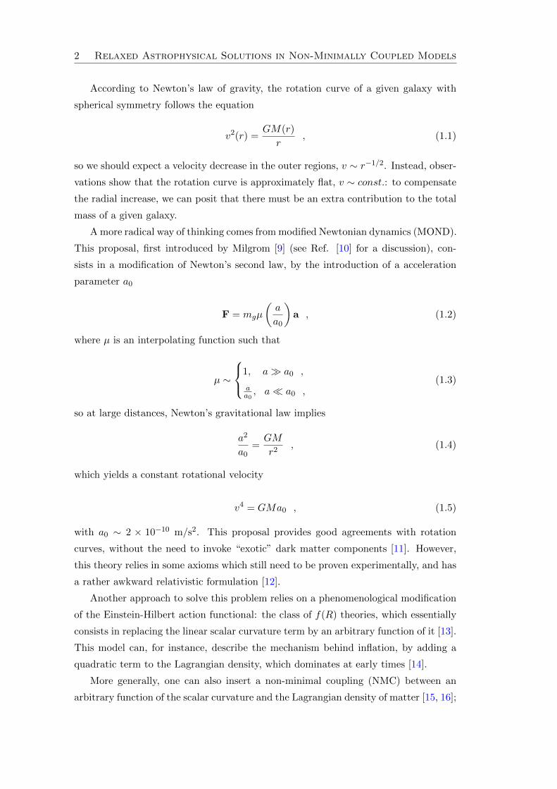
According to Newton’s law of gravity, the rotation curve of a given galaxy with

spherical symmetry follows the equation

v2(r) =GM(r)

r, (1.1)

so we should expect a velocity decrease in the outer regions, v ∼ r−1/2. Instead, obser-

vations show that the rotation curve is approximately flat, v ∼ const.: to compensate

the radial increase, we can posit that there must be an extra contribution to the total

mass of a given galaxy.

A more radical way of thinking comes from modified Newtonian dynamics (MOND).

This proposal, first introduced by Milgrom [9] (see Ref. [10] for a discussion), con-

sists in a modification of Newton’s second law, by the introduction of a acceleration

parameter a0

F = mgµ

(a

a0

)a , (1.2)

where µ is an interpolating function such that

µ ∼

1, a a0 ,

aa0, a a0 ,

(1.3)

so at large distances, Newton’s gravitational law implies

a2

a0=GM

r2, (1.4)

which yields a constant rotational velocity

v4 = GMa0 , (1.5)

with a0 ∼ 2 × 10−10 m/s2. This proposal provides good agreements with rotation

curves, without the need to invoke “exotic” dark matter components [11]. However,

this theory relies in some axioms which still need to be proven experimentally, and has

a rather awkward relativistic formulation [12].

Another approach to solve this problem relies on a phenomenological modification

of the Einstein-Hilbert action functional: the class of f(R) theories, which essentially

consists in replacing the linear scalar curvature term by an arbitrary function of it [13].

This model can, for instance, describe the mechanism behind inflation, by adding a

quadratic term to the Lagrangian density, which dominates at early times [14].

More generally, one can also insert a non-minimal coupling (NMC) between an

arbitrary function of the scalar curvature and the Lagrangian density of matter [15, 16];

1. Introduction 3

this can arise from one-loop vacuum-polarization effects in the formulation of Quantum

Electrodynamics in a curved space-time [17] or from considering a Riemann-Cartan

geometry [18]. In recent years, this theory has been carefully studied and has yielded

several interesting results [19–27], while avoiding potential pitfalls [28, 29] (see Ref.

[30] for a discussion).

Taking these considerations into account, in this thesis we aim to expand upon the

mechanism to mimic dark matter in the outer regions of galaxies resorting to a NMC

model in a relaxed regime, as first described in Ref. [31]. For simplicity, we restrict

the analysis to galaxies which exhibit spherical symmetry, composed of a perfect fluid.

The layout of this thesis is as follows: In Chapter 2, we give a motivation to the

use of NMC theories. In Chapter 3 we introduce the model under study and present

some of its properties. In Chapter 4, we delve in our calculations, starting by what

we call the “relaxed regime”, aiming to show that is possible to obtain an appropriate

dark matter mimicked profile for the model under scrutiny. In Chapter 5, we compare

our solutions with the standard models in the literature and constrain our parameters.

Finally, overall conclusions are presented in Chapter 6.

Chapter 2

General Relativity and

Alternative Theories of Gravity

In this chapter we start by introducing the Einstein-Hilbert action and then proceed

to derive the interior solution that describes the spacetime and energy structure of a

given object. Also, an introduction to conformal transformations will be given. Next,

we show how a conformal transformation induces an equivalence between GR and

the Jordan-Brans-Dicke theory. Later, we provide some introductory remarks about

phenomenological f(R) theories.

2.1 Einstein-Hilbert Action

Although Einstein’s theory of gravity was primarily constructed from the mathematical

description of differential manifolds, where the spacetime structure is non-Euclidean, it

can also be described through a Lagrangian formalism. Hilbert proposed the simplest

Lagrangian, so that the correspondent action functional reads

SEH =

∫d4x√−g (κR+ Lm) , (2.1)

where g denotes the determinant of the metric, κ = c4/16πG, where G is the gravita-

tional constant and c denotes the speed of light in vacuum and Lm is the Lagrangian

density of matter. From now on, we will take c = 1 unless stated otherwise.

Variation of the action functional with respect to the metric yields the Einstein

field equations

Gµν =8πG

c4Tµν , (2.2)

where Gµν is the Einstein tensor defined as

5

6 Relaxed Astrophysical Solutions in Non-Minimally Coupled Models

Gµν = Rµν −1

2gµνR , (2.3)

while Tµν is the energy-momentum tensor defined as

Tµν = − 2√−g

δ(√−gLm)

δgµν. (2.4)

2.2 Birkhoff Metric

One of the outstanding results concerning the structure of spacetime in General Rel-

ativity comes from the Birkhoff Theorem: it states that any spherically symmetric

solution of the vacuum field equations possesses a timelike Killing vector. The mathe-

matical structure behind this theorem is composed by four Killing vector fields ξµ i.e.,

vectors that satisfy the Killing equation:

∇µξν = −∇νξµ , (2.5)

where ∇µ is the covariant derivative. Three of these vectors are spacelike and, for

a spherical symmetric object, they are isomorphic to the generators of SO(3), the

rotation group, and satisfy the closed Lie algebra

[Li, Lj ] = εijkLj , (2.6)

where εijk is the Levi-Civita tensor. They are defined as

L1 = ∂φ , (2.7)

L2 = cosφ ∂θ − cot θ sinφ ∂φ , (2.8)

L3 = − sinφ ∂θ − cot θ cosφ ∂φ . (2.9)

The line element under these generators is written as

dΣ2 = dθ2 + sin2 θdφ2 , (2.10)

which produces the unit sphere S2.

In a four-dimensional spacetime, we can write the line element as

ds2 = −e2φ(r,t)dt2 + e2λ(r,t)dr2 + r2dΣ2 , (2.11)

2. General Relativity and Alternative Theories of Gravity 7

where φ(r, t) and λ(r, t) are arbitrary functions. The last Killing vector is obtained by

solving the Einstein field equations in vacuum, i.e. by setting Tµν = 0 in Eq. (2.2).

The relevant components are given by

Rtr =2

r∂tλ = 0 , (2.12)

which sets λ(t, r) = λ(r). The other one is

Rθθ = e−2λ [r(∂rλ− ∂rφ)− 1] + 1 = 0 . (2.13)

Differentiating with respect to time, this yields

∂t∂rφ = 0→ φ(r, t) = f(r) + g(t) . (2.14)

So that gtt = −e2f(r)e2g(t). Noting that we can always redefine our time coordinate as

dt→ e−g(t)dt and, setting g(t) = 0, we finally obtain the eponymous Birkhoff metric:

ds2 = −e2φ(r)dt2 + e2λ(r)dr2 + r2dΣ2 , (2.15)

we see that our metric elements are time independent, which implies that the last

Killing vector field is timelike.

2.3 Interior Solutions

One of the most interesting and fundamental results regarding GR lies in the solutions

which describe the interior of a spherical symmetric object, like a star.

We consider that our object is described by a perfect and isotropic fluid

Tµν = (p+ ρ)uµuν + pgµν , (2.16)

where ρ = ρ(r) denotes the energy density, p = p(r) the pressure, and uµ the 4-velocity

vector field, with components uµ = (u0, 0, 0, 0) (assuming the fluid at rest), normalized

uµuµ = −1 and with a vanishing gradient field: uµ∇νuµ = 0. Notice that, since the

energy-momentum tensor is diagonal and time independent, the Birkhoff metric (2.15)

can be adopted to this model.

Taking the trace of the Einstein field equation (2.2) we find that

R = −8πGT , (2.17)

8 Relaxed Astrophysical Solutions in Non-Minimally Coupled Models

so that Eq. (2.2) can be written as:

Rµν = 8πG

(Tµν −

1

2gµνT

). (2.18)

The non-vanishing and independent components of this equation are

e−2λ

(φ′′ + (φ′)2 − φ′λ′ + 2φ′

r

)= 4πG(3p+ ρ) , (2.19)

− e−2λ

(φ′′ + (φ′)2 − φ′λ′ − 2λ′

r

)= 4πG(ρ− p) , (2.20)

e−2λ

(λ′ − φ′

r

)+

1− e−2λ

r2= 4πG(ρ− p) . (2.21)

Adding (2.19) and (2.20) yields

e−2λ

(φ′ + λ′

r

)= 4πG(ρ+ p) . (2.22)

Now, adding (2.22) and (2.21) in order to eliminate φ′ and p, one has

e−2λ

(2λ′

r− 1

r2

)+

1

r2= 8πGρ . (2.23)

Given the background knowledge of the Schwarzchild solution, we re-define our metric

component grr as

e−2λ(r) = 1− 2Gm(r)

r. (2.24)

Physically, this can be seen as a straightforward extension of the Schwarzchild metric

to the interior of an object. Noticing that

e−2λ

(2λ′

r− 1

r2

)+

1

r2=

2Gm′

r2, (2.25)

Eq. (2.23) becomes

m′ = 4πρr2 , (2.26)

which, upon integration, yields

m(r) = 4π

∫ρ(r′)r′2dr′ . (2.27)

Thus confirming that m(r) gives the enclosed mass within a sphere of radius r. Sub-

tracting (2.22) with (2.21) in order to eliminate λ′ and ρ, yields after some algebra,

the relation

φ′ = G4πpr3 +m

r(r − 2Gm), (2.28)

2. General Relativity and Alternative Theories of Gravity 9

which, upon integration, defines the element gtt as

e2φ(r) = exp

(2G

∫4πp(r′)r′3 +m(r′)

r′ (r′ − 2Gm(r′))dr′)

. (2.29)

Thus, we can entirely define the spacetime geometry in terms of physical variables.

Obviously, pressure and energy density profile are still to be known. However, there is

still one last equation which can reduce our problem to a single degree of freedom. This

equation can be found in the conservation of the energy momentum tensor. Taking the

covariant derivative of the Einstein field equation (2.2) and resorting to the Bianchi

identity ∇µGµν = 0, one has

∇µTµν = 0 , (2.30)

taking the only non trivial component, ν = r, yields

φ′ = − p′

ρ+ p, (2.31)

which essentially sets a drag force due to the pressure gradient of the fluid. Replacing

this in (2.28), one thus arrives at the Tolman-Oppenheimer-Volkoff (TOV) equation,

the relativistic version of the hydrostatic equilibrium equation:

p′ = −(ρ+ p)4πGpr3 +Gm

r(r − 2Gm). (2.32)

Since Eqs. (2.27) and (2.32) form a system of two equations for three variables, to

solve this explicitly we need to give some a priori information for the system under

scrutiny: this can be supplied by an equation of state (EOS), p = p(ρ) that specifies

the intrinsic behavior of the assumed matter type.

2.4 Conformal Transformations

Given the metric gµν , a conformal transformation is defined as

gµν(x) = Ω2(x)gµν(x) , (2.33)

with an inverse

gµν(x) = Ω−2(x)gµν(x) , (2.34)

where Ω(x) is the conformal factor. In here, we will concern our attention to the

simple case where Ω is a global conformal factor, i.e., a constant, which implies a

scaling transformation of the metric. Below, we will show that in order to have an

10 Relaxed Astrophysical Solutions in Non-Minimally Coupled Models

invariantly conformed theory of gravity a scalar field must be introduced, remarkably

yielding a Brans-Dicke theory of gravity. Setting Ω(x) ≡ Ω, a global conformal factor

simply implies a scaling property of the metric.

Considering the infinitesimal line element:

ds2 = gµν(x)dxµdxν , (2.35)

it is easy to see that it is transformed accordingly to:

ds2 = Ω2ds2 . (2.36)

It is important to remark that this transformation only affects spacetime structure,

i.e., the coordinates xµ remain fixed. Also, they preserve the angle between two

geodesics.

With the metric, we can calculate how the relevant quantities transform accord-

ingly. For the connection, we have

Γαµν = Γαµν , (2.37)

since Γ ∼ g−1∂g. This implies that the Riemann tensor also remains invariant under

this transformations

Rµναβ = Rµναβ , (2.38)

and so does the Ricci scalar

Rµν = Rµν . (2.39)

However, the Ricci scalar gets a multiplicative factor

R = gµνRµν = Ω−2gµνRµν = Ω−2R . (2.40)

Finally, the d’ Alembertian , is transformed accordingly to

= gµν∇µ∇ν = Ω−2gµν∇µ∇ν = Ω−2 . (2.41)

2.4.1 Energy-Momentum Tensor

Given the prescription above, it is interesting to see how the relevant physical quantities

transform. We start by writing the physical part of the action functional S, which

should be naturally invariant under these transformations, since it should not depend

on how we stretch or contract our manifold. We have that:

2. General Relativity and Alternative Theories of Gravity 11

S =

∫d4x√−gL . (2.42)

Noticing that, in 4-dimensions,√−g = Ω4√−g and imposing the invariance of the

action functional, one has

S = S →∫d4x√−gL =

∫d4x√−g(Ω4L) ≡

∫d4x√−gL , (2.43)

so the invariance of the action functional is ascertained if the Lagrangian density is

transformed as

L = Ω−4L . (2.44)

Given this, the energy-momentum tensor is conformally transformed as

Tµν = − 2√g

δ

δgµν

(√−gL

)= −Ω−2 2√

−gδ

δgµν(√−gL

)= Ω−2Tµν . (2.45)

As an standard example, let us consider the energy-momentum tensor of a perfect

and isotropic fluid:

Tµν = (ρ+ p)uµuν + pgµν . (2.46)

Considering that our fluid moves along a geodesic, so that

uµ =dxµds

= gµαdxα

ds, (2.47)

in the conformal frame, one has

uµ = gµαdxα

ds= Ωgµα

dxa

ds= Ωuµ . (2.48)

Thus, we get

Tµν = (ρ+ p) uµuν + pgµν = Ω2 [(ρ+ p)uµuν + pgµν ] , (2.49)

using Eq. (2.45), we have that

Ω−2 [(ρ+ p)uµuν + pgµν ] = Ω2 [(ρ+ p)uµuν + pgµν ] , (2.50)

and this is trivially satisfied if

12 Relaxed Astrophysical Solutions in Non-Minimally Coupled Models

ρ = Ω−4ρ , (2.51)

p = Ω−4p . (2.52)

2.5 Equivalence Between GR and a Scalar Field Theory

In Section 2.4, we saw how the relevant tensors and scalars of GR transform by per-

forming a conformal transformation of the metric. However, that was the simplest

case where the scaling parameter Ω simply implies a global rescaling of the metric.

A more general approach comes from taking a local conformal factor Ω = Ω(x). For

that purpose, we start by writing the D dimensional action functional in the so called

Einstein frame in vacuum as (see Ref. [32])

S =ε

2

∫dDx

√−gR , (2.53)

where

ε =1

4

D − 2

D − 1, (2.54)

where, in 4-dimensions, has units [M2]. For a local conformal factor, the Ricci scalar

and the metric determinant are transformed accordingly to

R = Ω−2

(R− 2(D − 1)

Ω

Ω− (D − 1)(D − 4)gµν

Ω,µΩ,ν

Ω2

), (2.55)

and

√−g = ΩD√−g , (2.56)

so that the action functional becomes

S =ε

2

∫d4x√−gΩD−2

(R− 2(D − 1)

Ω

Ω− (D − 1)(D − 4)gµν

Ω,µΩ,ν

Ω2

), (2.57)

which is clearly not conformally invariant, unless we take the particular case where

Ω = constant and D = 2.

In order to obtain a conformal invariant theory, we introduce a scalar field that

modifies the action functional (2.53) according to

S =ε

2

∫dDx

√−gRΦ2 . (2.58)

2. General Relativity and Alternative Theories of Gravity 13

This is the so called Jordan frame, where the scalar curvature is not decoupled from

other matter fields. Inserting once again our conformally transformed variables, with

the redefined scalar field

Φ = Ω2−D2 Φ , (2.59)

leads to the action functional

S =1

2

∫dDx√−gΦ2

[εR− D − 2

2

Ω

Ω− 1

4(D − 2)(D − 4)gµν

Ω,µΩ,ν

Ω2

]. (2.60)

Adding the dynamical term

SΦ = −1

2

∫dDx

√−gΦΦ , (2.61)

leads to

S =1

2

∫dDx

√−gΦ

(εRΦ− Φ

), (2.62)

which is in fact conformal invariant since

S =1

2

∫dDx√−gΦ (εRΦ−Φ) , (2.63)

under the correspondingly transformation law for the d’Alembertian operator. From

this we conclude that, in order to obtain a conformal invariant theory of gravity, one

must add a scalar field to the action functional with a specific coupling to curvature.

Another important aspect that arises from this formalism is the equivalence with

the Jordan-Brans-Dicke (JBD) theory of gravity [33]. To see this clearly, we note that,

for a scalar, the d’Alembertian can be written as

Φ =1√−g

∂µ(√−g∂µΦ

), (2.64)

so that

S =1

2

∫dDx√−gΦ

(εRΦ− 1√

−g∂µ(√−g∂µΦ

)), (2.65)

integrating the second term by parts, fixing the boundary at the infinity and using

Stoke’s theorem so that the boundary contribution leads to a zero result, yields

S =1

2

∫dDx√−g[εRΦ2 + ∂µΦ∂µΦ

], (2.66)

14 Relaxed Astrophysical Solutions in Non-Minimally Coupled Models

which strikingly resembles the JBD action after redefining the scalar field as Φ =√

Ψ.

Finally, notice that, for a constant scalar field Φ, we have

S =ε

2

∫dDx√−gRΦ2 , (2.67)

so that the Eintein-Hilbert action can be recovered if

εΦ2 = κ→ Φ ∝ 1√G

, (2.68)

which was the motivation behind the Jordan-Brans-Dicken theory to explain gravity,

i.e., this theory relies on a local gravitational constant G. Given this relation between

the Einstein and Jordan frame, we can change our perspective to say that, in order to

go from one frame to another, a conformal transformation must be performed.

2.6 f(R) Action

It is suggestive, from a phenomenological point of view, that, instead of a trivial linear

contribution of the scalar curvature to the Lagrangian, one instead replaces it by a

arbitrary function of it. In this class of modified theories of gravity known as f(R)

models, the action functional is written as

Sf(R) =

∫d4x√−g [κf(R) + Lm] . (2.69)

The variation of action functional with respect to the metric yields the modified

field equation

2κF (R)Gµν − κ[f(R)−RF (R)]gµν = 2κ∆µνF (R) + Tµν , (2.70)

where F (R) ≡ df/dR and ∆µν ≡ ∇µ∇ν − gµν. As expected, GR can be recovered

by setting f(R) = R. Notice that the conservation of energy-momentum tensor is still

obeyed.

Taking the trace of the last equation, we have

κF (R)R− 2κf(R) = 3κF (R) + T , (2.71)

so for a de Sitter expansion, R = const and neglecting forms of matter T = 0, yields

F (R)R− 2f(R) = 0 , (2.72)

which has a trivial solution given by f(R) = αR2. This was first studied by Starobinsky

as an inflationary model [14].

2. General Relativity and Alternative Theories of Gravity 15

2.6.1 Equivalence Between f(R) and Scalar Field Theory

In Section 2.5 we saw that a local conformal transformation of the Einstein-Hilbert

action yields an equivalence between GR and a scalar field with a conformal coupling

and JBD theories. In f(R) models, this can also be ascertained (see, for example, Ref.

[34]): following the literature in [13], we start by deducing the action in the Jordan’s

frame, which can be done by inserting an auxiliary scalar field in the action functional

S =

∫d4x√−g [κ(f(χ) + f,χ (R− χ)) + Lm(gµν ,Ψm)] , (2.73)

where the Lagrangian density of matter not only depends on generic matter fields Ψm,

but also on the metric. Variation with respect to the χ, yields the field equation

f,χχ(χ)(R− χ) = 0 , (2.74)

for f,χχ = 0, R 6= χ, we recover the Einstein-Hilbert action with a constant contribu-

tion, since f(χ) = A + Bχ cancels out the linear scalar field contribution term. For

R = χ and provided that f,χχ 6= 0, the action (2.69) is recovered. Defining the scalaron

scalar field as

ψ = f,χ(χ) , (2.75)

we write the action as

S =

∫d4x√−g [κψR− U(ψ) + Lm(gµν ,Ψm)] , (2.76)

where

U(ψ) = κ [χ(ψ)ψ − f(χ(ψ))] , (2.77)

the action above resembles the one in JBD theory without a kinetic term and an

additional effective potential due to the scalaron: this is the so called O’Hanlon action

[35].

We now transform the action to the Einstein frame, where the scalar curvature

appears uncoupled. Performing a conformal transformation in the same fashion as

(2.33) and inverting Eq. (2.55) for D = 4, we have

S =

∫d4x√−g[κψΩ−2

(R+ 6

Ω

Ω− 6gµν

Ω,µΩ,ν

Ω2

)−

Ω−4U + Ω−4Lm(Ω−2gµν ,Ψm)],

(2.78)

16 Relaxed Astrophysical Solutions in Non-Minimally Coupled Models

defining our conformal factor as Ω2 = ψ and redefining the scalaron through

φ =√

3κ lnψ =√

12κ ln Ω , (2.79)

the action functional yields

S =

∫d4x√−g[κR− 1

2gµνφ,µφ,ν − V (φ) + e

−2φ√3κLm(e

−φ√3κ gµν ,Ψm)

], (2.80)

where

V (φ) =U

ψ2=ψR− fψ2

, (2.81)

and the Lagrangian density of matter is accordingly affected by the conformal trans-

formation of the metric: gµν = eφ√3κ gµν .

In conclusion, for the class of f(R) theories, the Einstein and Jordan frames are

also equivalent, provided that we add an extra scalar field φ to the action functional.

Chapter 3

Non-Minimal Coupling Model

Having introduced the so-called f(R) theories in the previous chapter, we now extend

this proposal to include an arbitrary non-minimal coupling between curvature and

matter.

3.1 Field Equations

For the purpose stated above, we opt for a Lagrangian density of the form

S =

∫d4x√−g [κf1(R) + f2(R)Lm] . (3.1)

The variation of the action with respect to the metric can be written as

δS =

∫d4x

[f2δ(√−gLm

)+ κδ

√−gf1

]+

∫d4x√−g [κF1 + F2Lm] δR , (3.2)

where, Fi ≡ dfi/dR, (i = 1, 2). Taking into account that

δ√−g = −1

2

√−ggµνδgµν , (3.3)

δR = Rµνδgµν −∆µνδg

µν , (3.4)

Tµν = − 2√−g

δ (√−gLm)

δgµν, (3.5)

the action can be written as

δS = −1

2

∫d4x√−g [f2Tµν + f1gµν ] δgµν (3.6)

+

∫d4x√−g [κF1 + F2Lm]Rµνδg

µν

−∫d4x√−g [κF1 + F2Lm] ∆µνδg

µν .

17

18 Relaxed Astrophysical Solutions in Non-Minimally Coupled Models

Fixing the boundary of our manifold at infinity, integrating twice by parts the last

contribution of (3.6), using Stoke’s theorem and finally evoking the Principle of least

action, we arrive at the field equation written below

2(κF1 + F2Lm)Gµν − [κ(f1 − F1R)− F2RLm]gµν = f2Tµν + 2∆µν(κF1 + LmF2) .(3.7)

Naturally, in the particular case f1 = R, f2 = 1, the above collapse to the Einstein

field equations, while f1(R) = f(R), f2(R) = 1 yields the equation of motion of f(R)

theories.

3.2 Non-Conservation of Energy-Momentum Tensor

One of the main features regarding the class of NMC theories is that the energy-

momentum tensor may not be covariantly conserved. This can be seen by resorting to

the Bianchi equation and the relation

(∇ν −∇ν)f = Rµν∇µf , (3.8)

which arises by resorting to the definition of Riemann tensor. Applying it to Eq. (3.7)

yields

∇µTµν =F2

f2(Lmgµν − Tµν)∇µR , (3.9)

which is clearly non conservative. Trivially, the conservation of the energy momentum

tensor can be ascertained by considering a minimal coupling f2(R) = 1. Other hy-

pothesis come from constraining our Lagrangian density such that Lmgµν = Tµν ; this,

however, cannot be assumed for all matter types, and indeed this non-conservation is

an intrinsic feature of the model [36]. From a cosmological perspective, the energy is

conserved by taking the Lagrangian density of a perfect fluid, Lm = −ρ (see Ref. [37]).

Naturally, this non-conservation may imply that a test particle may deviate from

its geodesic motion. To see this clearly, we resort to the energy-momentum tensor

described in Eq. (2.16) and consider the projection operator

Pλν = uλuν + gνλ . (3.10)

Contracting this tensor with Eq. (3.9) yields the modified geodesic equation

(ρ+ p)uµ∇µuλ = −Pλβp,β +F2

f2(uλu

α + δαλ ) (Lm − p)R,α , (3.11)

which, can be written as, in a more natural form,

3. Non-Minimal Coupling Model 19

duλds− Γσµλu

µuσ = fλ , (3.12)

where

fλ = −Pλβp,β

ρ+ p+F2

f2(uλu

α + δαλ )Lm − pρ+ p

R,α , (3.13)

so that, besides the usual force imposed by the gradient pressure of the fluid, an extra

contribution arises from the NMC. Notice that this extra contribution can be set to

zero if the assumed matter type has a Lagrangian density Lm = p. Finally, notice that

this force is perpendicular to the flow direction of the fluid, i.e., fλuλ = 0.

3.3 Choice of the Lagrangian

As we can see in Eq. (3.7), the equations of motion on NMC theories explicitly depends

on the Lagrangian density. In the perfect fluid scenario, this choice is not unique (see

Refs. [37, 38]).

To see this clearly, we start by writing an EOS for the energy density, ρ = ρ(n, s)

as a function of the particle density n and the entropy per particle s under the identi-

fication of the First Law of Thermodynamics

dρ = µdn+ nTds , (3.14)

where µ is the chemical potential defined as

µ ≡ ρ+ p

n. (3.15)

Next, we introduce the flux vector of the particle density

Jµ =√−gnuµ , (3.16)

which under the normalization uµuµ = −1, allow us to define the particle density

as n = |J |/√−g, with |J | ≡

√−gµνJµJν . Finally, we write the action functional

by inserting Lagrange coordinates αA and spacetime scalars φ, θ and βA in order to

enforce constrains on the fluid’s physical variables

S =

∫d4x[−

√−gρ(|J |/

√−g, s) + Jµ(φ,µ + sθ,µ + βAα

A,µ)] , (3.17)

where the index A takes the values 1, 2, 3. Taking into account the definition of the

energy-momentum tensor

20 Relaxed Astrophysical Solutions in Non-Minimally Coupled Models

Tµν =−2√−g

δ (√−gLm)

δgµν, (3.18)

the variation with respect to the metric yields

Tµν = ρuµuν +

(n∂ρ

∂n− ρ)

(gµν + uµuν) , (3.19)

so that the pressure is defined as

p = n∂ρ

∂n− ρ . (3.20)

Direct computation show us that µ = ∂ρ/∂n, the usual definition for the chemical

potential. The variation with respect to Jµ, φ, θ, s, αA and βA, yields the constrains

δS

δJµ= µuµ + φ,µ + sθ,µ + βAα

A,µ = 0 , (3.21)

δS

δφ= −Jµ;µ = 0 , (3.22)

δS

δθ= −(sJµ);µ = 0 , (3.23)

δS

δs= −

√−g∂ρ

∂s+ θ,µJ

µ = 0 , (3.24)

δS

δαA= − (βAJ

µ);µ = 0 , (3.25)

δS

δβA= αA,µJ

µ = 0 , (3.26)

so that, for example, Eq. (3.22) states that the flux / particle density is conserved.

Inspection of Eq. (3.24), show us that, after replacing the definition of density flux,

we have

∂ρ

∂s= nθ,µu

µ , (3.27)

since the temperature is related to the number of particles by

1

n

∂ρ

∂s

∣∣∣n

= T , (3.28)

the temperature may be alternatively defined with respect to the Lagrange multiplier

θ as T ≡ θ,µuµ. Finally, notice that by solving Eq. (3.21) with respect to the 4-velocity

and taking into the account the definition of the chemical potential (3.15), the action

reduces to

S =

∫d4x√−gp , (3.29)

3. Non-Minimal Coupling Model 21

one of the standard choices of the Lagrangian density [39]. Notice that in order to

obtain the constrains (3.21)-(3.26), the pressure must depend on the Lagrangian mul-

tipliers and the vector flux Jµ.

Now, the Lagrangian density that reproduces the Eq. (2.16) is not unique. Suppose

that, instead of starting with the action functional described in Eq. (3.17), we started

with

S =

∫d4x

[−√−gρ(n, s)− φJµ;µ − θ(sJµ);µ − αA(βAJ

µ);µ

], (3.30)

noticing that the satisfy the constrains (3.21)-(3.26), the action functional reduces to

S = −∫d4x√−gρ(n, s) , (3.31)

which, again, reproduces the energy-momentum tensor of a perfect fluid. With this,

we hence conclude that the Lagrangian choice is not unique, implying a degeneracy lift

of it, which may yield different physical systems. Finally, although not discussed here,

there is still, at least, another Lagrangian density which gives us the energy-momentum

tensor of a perfect fluid, Lm = na, where a is the physical free energy. Interestingly

enough, it was shown that for a linear coupling between matter and geometry, the mass

function of a star is strikingly similar regardless the Lagrangian density form (see Ref.

[23]).

3.4 Equivalence Between NMC and Scalar Field Theory

By the same token as in GR and f(R) theories, there is an equivalence between NMC

and scalar field theory [40]. Due to the coupling between matter and geometry, we only

need to notice that another scalar field must be introduced in the action functional

S =

∫d4x√−g [κf1(χ) + ψ(R− χ) + f2(χ)Lm(gµν ,Ψm)] , (3.32)

so that the actional functional in the Jordan frame can be written as

S =

∫d4x√−g [ψR− V (χ, ψ)− f2(χ)Lm(gµν ,Ψm)] , (3.33)

where

V (χ, ψ) = ψχ− κf1(χ) , (3.34)

with ψ and χ satisfying the field equations

χ = R , (3.35)

22 Relaxed Astrophysical Solutions in Non-Minimally Coupled Models

ψ = κF1(χ) + LF2(χ) . (3.36)

The potential V (χ, ψ) can be seen as the interaction potential between these two

fields. Equivalently, the Einstein frame can be recovered by performing the conformal

transformation described in Section 2.6.1, which yields

S =

∫d4x√−g[Ω−2ψ

(R+ 6

Ω

Ω− 6gµν

Ω,µΩ,ν

Ω2

)−

Ω−4ψ2U + Ω−4f2(χ)Lm(Ω−2gµν ,Ψm)],

(3.37)

where U ≡ ψ−2V . Defining

ψ = Ω2 , (3.38)

and

φ =√

3κ lnψ , (3.39)

we find that

S =

∫d4x√−g[R− 1

2κgµνφ,µφ,ν − U + e

−2φ√3κ f2(χ)Lm(e

−φ√3κ gµν ,Ψm)

], (3.40)

where the metric in the Einstein frame is again related to the physical one by a scalar

field: gµν = eφ√3κ gµν .

Chapter 4

Relaxed Non-Minimally Coupled

Regime

Having presented a brief introduction to the class of modified theory of gravity with

a non-minimal coupling, we begin to develop the main work of this thesis. For that,

we follow Refs. [31, 41], where it was shown that under a certain class of coupling

functions, it is possible to mimic dark matter in the outer regions of galaxies with

approximately spherical symmetry. For this, we impose that

κF1 + F2Lm = Ωκ , (4.1)

where Ω is a constant to be determined. This condition fixes what we call the relaxed

regime for the NMC. Notice that this condition can be straightforwardly interpreted

in the Jordan frame, by comparing it to Eq. (3.36) and setting ψ = Ωκ.

This restriction can be seen as a fixed point condition, since the ∆µν term on the

field equations (3.7) vanishes accordingly. Indeed, in a cosmological context it was

found that Eq. (4.1) arises naturally from a dynamical system formulation [42, 43],

allowing for a de Sitter expansion of the Universe in the presence of a non-negligible

matter content; a previous effort had shown that Eq. (4.1) leads to interesting modi-

fications of the Friedmann equation [41] (see Ref. [19] for similar results).

In an astrophysical context, one can interpret it as a way to mimic dark matter

[27, 31]. First used in Ref. [31], the above provides an immediate relation for ρ = ρ(R)

in the case of a pressureless dust distribution; that study also showed that numerical

solutions to the overall field equations admit solutions that have very small oscillations

around the latter.

Condition (4.1) acts as an additional constraint R = R(Lm) to the ensuing system

of differential equations: as such, an extra equation of state (EOS) is no longer required

23

24 Relaxed Astrophysical Solutions in Non-Minimally Coupled Models

a priori: instead, one may in principle solve the full set of equations and then read the

corresponding EOS parameter ω(ρ) = p(ρ)/ρ from it.

Inserting (4.1) into the field equations (3.7) leads to the simplified form

Rµν =1

2Ωκ(f2Tµν + κf1gµν) . (4.2)

The ensuing trace yields

R =1

2Ωκ(f2T + 4κf1) , (4.3)

so that solving it for f1 and replacing into (4.2), one finally arrives at the traceless

form

Rµν −1

4Rgµν =

f2

2Ωκ

(Tµν −

1

4Tgµν

), (4.4)

which is strikingly similar to Unimodular gravity [44], although complemented by an

NMC.

4.1 Dark Matter Mimicking

As we stated, the main objective of this work is to mimic dark matter through a

NMC between curvature and visible matter. Given the relation R = R(Lm) that

arises from the relaxed regime (4.1), we thus interprets the additional contributions

to the field equations (4.4) as an effective dark matter: to ascertain this, we write

the latter as the usual Einstein field equations with an additional energy-momentum

tensor contribution for dark matter,

2κGµν = T (dm)µν + Tµν . (4.5)

Assuming that the latter also behaves as a perfect fluid,

T (dm)µν = (ρdm + pdm)vµvν + pdmgµν , (4.6)

with vµ = uµ (so that this mimicked dark matter is “dragged” by visible matter), one

can easily arrive at

pdm =

(f2

Ω− 1

)ωρ− f2T

4Ω− κR

2,

ρdm =

(f2

Ω− 1

)ρ+

f2T

4Ω+κR

2. (4.7)

4. Relaxed Non-Minimally Coupled Regime 25

In the case of GR, this component naturally vanishes due to the usual trace con-

dition R = −T/2κ and the minimal coupling f2(R) = 1 (after imposing Ω = 1).

4.2 Stationary Case

In this section we obtain a system of differential equations to our variables of interest.

Assuming spherical symmetry and stationarity, we adopt the Birkhoff metric (2.15),

here repeated for convenience:

ds2 = −e2φ(r)dt2 + e2λ(r)dr2 + r2dΣ2 . (4.8)

The non-vanishing components of the energy-momentum tensor of matter (2.16)

can be easily evaluated,

Ttt = ρe2φ, Trr = pe2λ, Tθθ = pr2 , (4.9)

with trace T = 3p− ρ.

Given that a perfect fluid is described by a Lagrangian density L = −ρ [37, 38],

while radiation obeys L = p, we adopt the general description

Lm = −γρ =

−ρ , γ = 1

p , γ = −ω. (4.10)

Taking the radial component of Eq. (3.9), we find

φ′(ρ+ p) =F2

f2(Lm − p)R′ − p′ . (4.11)

Notice that the previous equation resembles Eq. (2.31), with the extra contribution

due to the NMC. Replacing the form of the Lagrangian, we have

φ′ = −βF2

f2R′ − 1

ω + 1

(ω′ + ω

ρ′

ρ

), (4.12)

with the binary parameter

β =γ + ω

1 + ω=

1 , γ = 1

0 , γ = −ω, (4.13)

introduced for convenience.

We now address the field equation (4.4), resorting to the relation

gttRtt − grrRrr = −2

re−2λ

(φ′ + λ′

), (4.14)

26 Relaxed Astrophysical Solutions in Non-Minimally Coupled Models

which, for the adopted diagonal metric, implies that

e−2λ

(φ′ + λ′

r

)=ω + 1

4Ωκf2ρ . (4.15)

The other independent component comes from taking θ − θ in (4.4), which reads

e−2λ

r

(λ′ − φ′

)− e−2λ

r2+

1

r2=R

4+ω + 1

8Ωκf2ρ . (4.16)

Now, we solve Eq. (4.15) for λ′(r) yielding

λ′ =1 + ω

4Ωκf2ρe

2λr − φ′ . (4.17)

Inserting this result into Eq. (4.16) allow us to define grr as

e2λ =1 + 2rφ′

1− r2

4

(R− 1+ω

2Ωκ f2ρ) . (4.18)

Taking into the account the expression for the scalar curvature

e2λ

2R =

e2λ − 1

r2+

(2

r+ φ′

)(λ′ − φ′

)− φ′′ , (4.19)

and replacing the two preceding expressions for e2λ and λ′ into it we find that

(1 + 2rφ′)

[1 + ω

2Ωκf2ρ

(1 +

r

2φ′)− R

2+

1

r2

]= (4.20)[

1

r2+

4

rφ′ + 2(φ′)2 + φ′′

] [1− r2

4

(R− 1 + ω

2Ωκf2ρ

)].

Simplifying both sides, we can write the last equation as

R

8− 3

8

1 + ω

Ωκf2ρr

(1

2r+ φ′

)+φ′

r− 1 + ω

8Ωκf2ρr

2

((φ′)2 − φ′′

2

)(4.21)

+

(1− R

4r2

)((φ′)2 +

φ′′

2

)= 0 .

Notice that, for consistency, one could obtain the same expression by differentiating

Eq. (4.18) and inserting Eq. (4.17) into it.

Differentiating φ′ with respect to the radial coordinate, yields

φ′′ = β

[(F2

f2

)2

(R′)2 − F ′2f2

(R′)2 − F2

f2R′′

]+

ω′

(1 + ω)2

[ω′ + ω

ρ′

ρ

](4.22)

− 1

1 + ω

[ω′′ + ω′

ρ′

ρ− ω

(ρ′

ρ

)2

+ ωρ′′

ρ

],

4. Relaxed Non-Minimally Coupled Regime 27

and replacing φ′ and φ′′ into Eq. (4.21), we finally arrive at the cumbersome expression

below,

3

8

1 + ω

Ωκf2ρr

[1

2r− βF2

f2R′ − 1

ω + 1

(ω′ + ω

ρ′

ρ

)]+

1

r

1

ω + 1

(ω′ + ω

ρ′

ρ

)+

β

r

F2

f2R′ +

1 + ω

8Ωκf2ρr

2

[β

(β − 1

2

)(F2

f2

)2

(R′)2 +β

2

F ′2f2

(R′)2 +β

2

F2

f2R′′

+1

2

ω

1 + ω

ρ′′

ρ+

1 + 4ω

2(1 + ω)2

ρ′

ρω′ +

(ω′)2 + (1 + ω)ω′′

2(1 + ω)2+ ω

ω − 1

2(ω + 1)2

(ρ′

ρ

)2

+ 2β1

1 + ω

F2

f2R′(ωρ′

ρ+ ω′

)]−[1− R

4r2

][β

(β +

1

2

)(F2

f2

)2

(R′)2

− β

2

F ′2f2

(R′)2 − β

2

F2

f2R′′ + ω

3ω + 1

2(ω + 1)2

(ρ′

ρ

)2

+3(ω′)2 − (1 + ω)ω′′

2(1 + ω)2

− 1

2

ω

1 + ω

ρ′′

ρ+

4ω − 1

2(1 + ω)2ω′ρ′

ρ+ 2β

1

1 + ω

F2

f2R′(ωρ′

ρ+ ω′

)]− R

8= 0 , (4.23)

a second order and non-linear differential equation for three variables ρ(r), ω(r) and

R(r).

4.3 Analytical Solution

We now aim to solve the above differential equation. First, we simplify it by defining

the dimensionless variables

x ≡ r√R2 , y ≡ R

R2, % ≡ ρ

2κR2, (4.24)

where R2 is an as of yet arbitrary curvature scale that, as we shall see, equates with

the characteristic curvature scale of the NMC. Given this, the relaxed regime condition

(4.1) and trace Eq. (4.3) can be written as

Ω = F1 − 2γF2R2% , (4.25)

Ωy = f2(3ω − 1)%+2f1

R2,

while the differential equation (4.23) yields

28 Relaxed Astrophysical Solutions in Non-Minimally Coupled Models

3(1 + ω)f2%

Ωx

[1

x− 2β

F2R2

f2y′ − 2

ω + 1

(ω′ + ω

%′

%

)]+

8β

x

F2R2

f2y′

+8

x

1

ω + 1

(ω′ + ω

%′

%

)+ (1 + ω)

f2%

Ωx2

[β (2β − 1)

(F2R2

f2

)2

(y′)2

+ βF ′2R

22

f2(y′)2 + β

F2R2

f2y′′ +

(ω′)2 + (1 + ω)ω′′

(1 + ω)2+ ω

ω − 1

(ω + 1)2

(%′

%

)2

+ω

1 + ω

%′′

%+

1 + 4ω

(1 + ω)2

%′

%ω′ + 4β

1

1 + ω

F2R2

f2y′(ω%′

%+ ω′

)]−

[4− yx2

] [β (2β + 1)

(F2R2

f2

)2

(y′)2 − βF′2R

22

f2(y′)2 − βF2R2

f2y′′

+3(ω′)2 − (1 + ω)ω′′

(1 + ω)2+ ω

3ω + 1

(ω + 1)2

(%′

%

)2

− ω

1 + ω

%′′

%+

4ω − 1

(1 + ω)2ω′%′

%

+ 4β1

1 + ω

F2R2

f2y′(ω%′

%+ ω′

)]− y = 0 . (4.26)

where the derivatives are now with respect to x. In order to proceed with our calcu-

lations, we need to give explicit expressions to fi(R). Following Ref. [31], we assume

a trivial f1(R) and a power law for the NMC of the form

f1(R) = R ,

f2(R) = 1 +

(R

R2

)n, (4.27)

where R2 is a characteristic curvature scale. With the choice of the Lagrangian density

of a perfect fluid Lm = −ρ→ γ = 1, conditions (4.25) read

1− Ω

2ny1−n = % , (4.28)

(Ω− 2)y = (1 + yn)(3ω − 1)% .

Regarding the fixed point condition, in Ref. [31] it was found that the energy density

and curvature were related by

R =1− 2n

2κ

(R

R2

)nρ , (4.29)

which, written in terms of the dimensionless variables (4.24), reads

1

1− 2ny1−n = % . (4.30)

4. Relaxed Non-Minimally Coupled Regime 29

Matching both results, we fix our constant Ω as

Ω =1− 4n

1− 2n. (4.31)

With this, the conditions above translate into

y1−n = (1− 2n)% , (4.32)

y = (1− 2n)(1 + yn)(1− 3ω)% .

Furthermore, notice that the set of relations

f2 = 1 + yn ,

F2R2

f2= n

yn−1

1 + yn, (4.33)

F ′2R22

f2= n(n− 1)

yn−2

1 + yn,

are only dependent on the power law exponent n.

We are finally in position to solve our differential equation under the appropriate

conditions. For that purpose, we notice that visible matter is non-relativistic, so that

the EOS parameter should be small, ω ∼ 0. With this condition, solving the trace in

Eq. (4.32) for the EOS parameter yields

yn = (1 + yn)(1− 3ω)y1−n → yn =1

3ω− 1 ∼ 1

3ω, (4.34)

so that the vanishingly small pressure of visible matter translates into the dominance

of the NMC term, ω ∼ 0→ yn ∼ f2 1; since we consider a negative exponent n < 0,

this translates into a very small reduced curvature y 1.

Given this, the visible matter density ρ and EOS parameter ω are written implicitly

in terms of the scalar curvature as

ρ =2κR2

1− 2n

(R

R2

)1−n, ω =

1

3

(R

R2

)−n, (4.35)

while the mimicked dark matter distribution are given by direct computation of Eqs.

(4.7) after replacing the expressions above and the fi functions in (4.27)

ρdm ∼ 1− n1− 4n

2κR , (4.36)

pdm ∼ n

1− 4n2κR ,

30 Relaxed Astrophysical Solutions in Non-Minimally Coupled Models

where we neglected the extra contributions which arise from the fluid’s pressure, which

are clearly perturbative by Eq. (4.35).

Given the low-curvature regime above, we attempt to solve the differential equation

(4.26) by resorting to the algebraic relations (4.32), (4.33) and (4.34). To do so, we

first solve it for y′′ and expand (4.26) perturbatively y ∼ 0 to first order, yielding the

considerably simplified equation

− 2y′(x)

x+ (1 + 2n)

y′(x)2

y(x)− y′′(x) = 0 . (4.37)

This non-linear second order differential equation has an analytical solution given

by

y(x) = yf

(2x

xf + x

) 12n

, (4.38)

where xf and yf are integration constants: it is easy to check that y(xf ) = yf , so this

normalization simply gives us the value of the scalar curvature evaluated at a given

radius; we choose to identify xf as the reduced radius of the visible part of a given

galaxy, while yf the correspondent value of the reduced scalar curvature.

In the asymptotic regime x xf , i.e. for a region sufficiently far away from our

galaxy, one has

y(x) ∼ 212n yf

(1− 1

2n

xfx

), (4.39)

so that the scalar curvature approaches the value

y(∞) ∼ 212n yf , (4.40)

which we interpret as the background contribution of the curvature.

Conversely, in the limit x xf , i.e. for regions where we aim to obtain a mimicked

dark matter halo, one has

y(x) ∼ yf(

2x

xf

) 12n

. (4.41)

The scalar curvature and the respective dark matter contributions can be explicitly

written as

R(r) = Rf

(2r

rf + r

) 12n

, (4.42)

ρdm(r) =1− n1− 4n

2κRf

(2r

rf + r

) 12n

,

pdm(r) =n

1− 4n2κRf

(2r

rf + r

) 12n

,

4. Relaxed Non-Minimally Coupled Regime 31

while visible matter is characterized by

ρ(r) =2κRf1− 4n

(RfR2

)−n( 2r

rf + r

) 1−n2n

,

ω(r) =1

3√

2

(RfR2

)−n√1 +

rfr

, (4.43)

where rf denotes a given boundary radius of the galaxy and Rf the correspondent

scalar curvature.

Chapter 5

Matter Profiles and Constrains

to the Model

In the previous chapter, we obtained an exact solution to the mimicked dark matter

profile for the halo region of a given galaxy. With this in mind, we now aim to compare

this solution with the standard profiles which can be found in the literature. Also, we

show that the energy conditions are satisfied under the appropriate range of values for

the power law exponent n. Finally, constraints to the non-minimal coupling parameter

will be given.

5.1 Standard Matter Profiles

Given the dark and visible matter energy density solutions, we start this new chapter

by comparing our solutions with the profiles of interest, namely the Hernquist, Navarro-

Frenk-White (NFW) [45] and isothermal [46] distributions. For that, we start by noting

that away from the boundary of the galaxy, r rf and we can use (4.42) to write

ρdm(r) ∼ 1− n1− 4n

2κRf

(2r

rf

) 12n

. (5.1)

Thus, we obtain a direct translation between the slope of the dark matter distri-

bution ρdm and the NMC exponent n. By the same token, the visible profile can also

be approximated in Eq. (4.43) by

ρ(r) ∼2κRf1− 4n

(RfR2

)−n(2r

rf

) 1−n2n

. (5.2)

33

34 Relaxed Astrophysical Solutions in Non-Minimally Coupled Models

5.1.1 Cusped Profiles

Along the years, an exhaustive attempt to theoretically find density profiles which de-

scribe dark matter has been pursued. Through N-body simulations and spectrography,

it was found that most models fit in a empirical density model, the so called cusped

profile [47]

ρ(r) =ρcp(

ra

)γ (1 + r

a

)m−γ , (5.3)

where ρcp denotes the density scale, a the transition radius between visible and dark

matter dominance and γ, m the inner and outer logarithmic slopes, respectively. This

profiles can model not only dark matter, but also the density profile of visible matter.

To determine the correspondent mass profile for the outer region, we start by taking

r a in (5.3),

ρ(r) ∼ ρcp(ar

)m, (5.4)

notice that the density is independent of the inner slope γ. Resorting to Eq. (2.27),

the mass profile is given by

M(r) =4π

3−mamρcpr

3−m , (5.5)

for m 6= 3.

To determine the rotational velocity, we invoke Newton’s law of gravitation and

find that

v2 =GM(r)

r=

4π

3−mamρcpr

2−m . (5.6)

We thus see that the outer logarithmic slope m regulates the asymptotic behavior of

the rotation curve, which is flat if m = 2, while different values of m translate into a

increasing or decreasing behavior, for m < 2 or m > 2, respectively.

5.1.2 Hernquist Visible Matter Profile

Historically, one of the outstanding candidates for density profile of visible matter is

the well known Hernquist profile [48],

ρHernq(r) =M

2πa3

1ra

(1 + r

a

)3 , (5.7)

which was initially introduced to solve the luminosity problem for elliptical galaxies. In

the previous equation, M denotes the total visible mass of a given galaxy. Comparing

5. Matter Profiles and Constrains to the Model 35

with the cusped profile, this is the particular case where γ = 1, m = 4 and ρcp =

M/(2πa3).

For the inner and outer regions, i.e., r a and r a, respectively, one has

ρHern(r) ∼ M

2πa3

ar , r a(ar

)4, r a

, (5.8)

so that comparing the outer region limit with Eq. (5.2), it is trivial to check that this

is realized by setting the NMC exponent nHernq = −1/7.

Resorting to Eq. (5.1), the correspondent DM profile translates into

ρdm =16κRf

11

(2r

rf

)− 72

. (5.9)

5.1.3 Navarro-Frenk-White Dark Matter Profile

Regarding dark matter density profiles, the first one considered here is the Navarro-

Frenk-White [45], which was introduced a priori in order to study N-body simulations

of dark matter halo in galaxies. It is given by

ρNFW (r) =ρcp

ra

(1 + r

a

)2 , (5.10)

and is a cusped profile with γ = 1,m = 3. Following the same procedure as before, we

have that

ρNFW (r) ∼ ρcp

ar , r a(ar

)3, r a

, (5.11)

comparing with (5.1), we find that nNFW = −1/6. Resorting to Eq. (5.2), the density

profile of visible matter translates into

ρ(r) ∼6κRf

5

(RfR2

)1/6(2r

rf

)−7/2

. (5.12)

5.1.4 Isothermal Dark Matter Profile

Finally, we have the isothermal profile, which is also used to model dark matter be-

havior in the outer regions. Mathematically, this can be obtained by considering a

polytropic equation of state p = Kρ and solving the hydrostatic equilibrium equation

dΦ

dr= −1

ρ

dp

dr, (5.13)

36 Relaxed Astrophysical Solutions in Non-Minimally Coupled Models

where Φ ≡ Φ(r) is the gravitational potential. Solving it for ρ, one has

ρI(r) =v2∞

2πGr2. (5.14)

It is a cusped profile with m = γ = 2, and the divergence at r = 0 leads it to being

called the singular isothermal profile, where v∞ is the asymptotically velocity, i.e., the

(constant) velocity for outer regions with the correspondence v2∞ = 2πGρcpa

2.

By the same token as before, one finds nI = −1/4 and the correspondent visible

density profile

ρ(r) = κRf

(RfR2

)1/4(2r

rf

)−5/2

. (5.15)

Finally, we summarize the characteristic behaviors for both dark and visible matter

density in Table. 5.1

Profiles n ρ(r) ρdm(r)

Hernquist −1/7 r−4 r−7/2

NFW −1/6 r−7/2 r−3

Isothermal −1/4 r−5/2 r−2

Table 5.1: Outer region behavior for the relevant profiles

To complete our discussion, we introduce some alternative models, such as the

Burkert profile [49]

ρB(r) = ρva3

(r + a)(r + a)2, (5.16)

where ρv = ρ(0), thus removing the core singularity. Notice that it resembles the NFW

profile for the outer regions (ρ ∼ r−3). With a different family of functions we have

the Einasto profile

ρ(r) = ρv exp

[−dp

([ra

]1/p− 1

)], (5.17)

where dp is an adequate function of p, such that r = a encloses half of the total mass;

and the deprojected Sersic law

ρ(r) = ρv

(ra

)−pmexp

[−dm

(ra

) 1m

], (5.18)

with pm and dm characteristic scales.

5. Matter Profiles and Constrains to the Model 37

5.2 Mass Budget

Since in Section 4.1 we imposed that the total contribution of dark and visible matter

to the energy momentum tensor satisfies the GR equation, we can simply cast the

metric elements which were found in Section 2.3,

m(r) = 4π

∫ρt(r)r

2dr ,

e2λ(r) =

(1− m(r)

8πκr

)−1

,

e2φ(r) = exp

(∫4πpt(r)r

3 +m(r)

r(8πκr −m(r))dr

), (5.19)

where ρt and pt denote, respectively, the total (visible + dark) energy density and

pressure. Regarding this, notice that we could always find the metric elements by using

the expressions found in Section 4.2: however, the above is clearly more convenient,

once the mimicked dark matter behavior has been written explicitly. Furthermore, it

is known that a galaxy is within the validity of the Newtonian regime, gµν ∼ ηµν .

5.2.1 Mass

When computing the mass of our spherical object, one needs to be careful with the

limits of integration: indeed, since the validity of our solution (4.38) is satisfied only in

the halo regions of our galaxy, we cannot simply integrate it from the center to a given

radius r. Hence, we define an inner radius a, in the same sense described in Section

5.1.1, i.e., the transition radius between dark and visible matter dominance.

Using the definition of mass in the first equation (5.19), one has that the mass

component Mi enclosed in the halo region a < r < rf is given by

Mi = 4π

∫ rf

aρi(r)r

2dr . (5.20)

Resorting once more to Eqs. (5.1) and (5.2)

ρ(r) ∼ 1

1− 4n2κR2

(RfR2

)1−n(2r

rf

) 1−n2n

,

ρdm(r) ∼ 1− n1− 4n

2κRf

(2r

rf

) 12n

, (5.21)

we find the contribution of dark matter mass to the galaxy halo,

Mdm = hnRfr

3fc

2

G

[1−

(a

rf

) 1+6n2n

], (5.22)

38 Relaxed Astrophysical Solutions in Non-Minimally Coupled Models

for n 6= −1/6, where

hn ≡2

12nn(1− n)

(1− 4n)(1 + 6n). (5.23)

Notice that in order to keep the mass positive defined, the condition n < −1/6 is

required.

For n = −1/6, it is easy to see that the dark matter mass has a logarithmic

dependence

Mdm =7

160Rfr

2f

rfc2

Gln(rfa

). (5.24)

For any value of the exponent n 6= −1/5 (which does not correspond to any profile

of interest and is thus disregarded), the visible mass enclosed within the mimicked

dark matter halo is given by

Mv = h′n

(RfR2

)−n Rfr3fc

2

G

[1−

(a

rf

) 5n+12n

], (5.25)

with

h′n ≡2

1−n2n n

(1− 4n)(1 + 5n). (5.26)

The ratio between dark matter and visible mass is thus

Mdm

Mv=hnh′n

(RfR2

)n 1−(arf

) 1+6n2n

1−(arf

) 1+5n2n

, (5.27)

for n 6= −1/6 and

Mdm

Mv=

7

6√

2

(R2

Rf

)1/6 ln( rfa

)√rfa − 1

, (5.28)

for n = −1/6. Since h′n ∼ hn and a . rf , the low-curvature regime (Rf/R2)n 1

implies that dark matter mass will dominate, as desired.

5.3 Energy Conditions

In this section, we focus our attention in the energy conditions. These can be obtained

by considering the Raychaudhuri equation in the case of a congruence of null geodesics

defined by a vector field kµ by (see, for example, Refs. [28, 50])

dθ

dτ= −1

2θ2 − σµνσµν + ωµνω

µν −Rµνkµkν , (5.29)

5. Matter Profiles and Constrains to the Model 39

where θ is the expansion parameter, σµν the shear and ωµν the rotation associated

with the congruence. This equation can describe, for instance, the change of volume

of a given ball for a co-moving observer in the center of it. Gravity remains attractive

as long as the variation of θ with respect to the proper time τ stays negative.

Since we interpret our model as equivalent to GR with the effect of the NMC

ascribed to an additional, effective, component that behaves as a perfect fluid, the

strong, null, weak and dominant energy conditions can be cast, respectively, as

ρt + 3pt ≥ 0 , SEC

ρt + pt ≥ 0 , NEC

ρt ≥ 0 , WEC

ρt ≥ pt ≥ −ρt , DEC

. (5.30)

In here, ρt and pt denote the total (visible + dark) energy density and pressure.

Since the low-curvature regimes induces a zero pressure and a perturbative energy

density, we can safely neglect both contributions.

Considering the dark matter components in Eq. (4.36), the SEC, NEC and WEC

can be summarized as (1− 2n

1− 4n

)(1 + En) ρ ≥ 0 , (5.31)

where

En =

2n , SEC

0 , NEC

−n , WEC

, (5.32)

while the DEC is satisfied if

0 ≥(

1− 2n

1− 4n

)(2n− 1) ≥ 2

(1− 2n

1− 4n

)(n− 1) . (5.33)

Thus, the SEC is satisfied for −1/2 ≤ n < 1/4, while the NEC, WEC and DEC

are satisfied for n < 1/4, which encompasses all the relevant visible and dark matter

profiles considered here.

5.4 Model Parameter Constraints

In this section, we aim to compare the expressions found in the section 5.2.1 with

observed values. Since our solutions were found by the assumption that our object

40 Relaxed Astrophysical Solutions in Non-Minimally Coupled Models

has spherical symmetry, we adopt the dataset reported in Refs. [51, 52] for galaxies of

type E0, which display low eccentricity. The relevant quantities (a, rf ) and enclosed

visible and dark matter masses (as inferred from the corresponding rotation curves)

are depicted in Table 5.2.

NGC Mv(1010M) Mdm(1011M) rf (kpc) a(kpc) yf (10−3)

2434 4.6 1.9 18 5.1 0.65846 36.4 8.5 70 21.1 2.16703 5.6 1.2 18 2.7 1.17145 3.8 1.4 25 4.0 0.47192 7.1 2.7 30 4.1 0.37507 7.9 3.5 18 4.7 0.37626 30.7 8.7 50 11.0 0.4

Table 5.2: Data obtained by performing a fit to rotational curves of galaxies.

Following this, a χ2 fitting procedure is followed to ascertain which parameters n

and R2 lead to the best fit of the mimicked dark matter to visible mass ratio (5.27)

and (5.28) to the values obtained from Table 5.2. For that purpose, one eliminates Rf

in this equations by resorting to (5.22) and (5.24) yielding, respectively

Mdm

Mv=h1−nn

h′n

(r2fR2

rfc2

GMdm

)−n [1−

(a

rf

) 5n+12n

]−1 [1−

(a

rf

) 6n+12n

]1−n

, (5.34)

for n 6= −1/6, and

Mdm

Mv=

7

12

(7

20

rfc2

GMdmr2fR2

)1/6 [ln ( rfa )]7/6√rfa − 1

, (5.35)

for n = −1/6. Following through with the numerical session, it is found that the value

for the adjusted correlation coefficient r2 increases as we arbitrarily approach n =

−1/6. The best fit is then found when n = −1/6, yielding a correlation coefficient r2 =

0.86: this relatively low value can be reflected by small deviations from sphericity in the

selected type E0 galaxies, as well as unmodeled localized features and inhomogeneities.

The best fit for the characteristic length scale was found to be R2 ≈ 5 Mpc−2, although

with a large uncertainty stemming from the relative lack of sensitivity of (5.35) to it:

as such, we are only allowed to conclude that R2 ∼ Mpc−2.

Finally, it is also interesting to see where the assumption behind the low-curvature

regime holds. For that, one resort to Eqs. (5.27) and (5.28) and solve it for Rf/R2.

5. Matter Profiles and Constrains to the Model 41

-0.25 -0.20 -0.15 -0.10

0.00

0.05

0.10

0.15

Figure 5.1: Plot of the low-curvature regime validation as a function of the powerlaw exponent n.

This yields

yf =

(Mdm

Mv

) 1n(h′nhn

) 1n

1−(arf

) 1+5n2n

1−(arf

) 1+6n2n

1n

, (5.36)

for n 6= −1/6, and

yf =

(7

6√

2

)6( Mv

Mdm

)6 ln

( rfa

)√rfa − 1

6

, (5.37)

for n = −1/6.

Focusing on Fig. 5.1, we see that the regime holds for the power law exponents

identified with the standard density profiles. However, as n decreases, the fitted curves

of each galaxy, which are representative of Eq. (5.36) tend to break the regime. The

black dots represents the different NGC galaxies for nNFW , where the values of yf are

given in the last column of Table 5.2, which are clearly perturbative.

Chapter 6

Conclusions

In this thesis, we showed that the rich phenomenology of a model endowed with a non-

minimal coupling between curvature and matter allows for the possibility of mimicking

dark matter profiles for galaxies which exhibit spheric symmetry. This result was

obtained by assuming a relaxed regime, interpreted as a fixed point condition, which

allowed us to relate the Lagrangian density with the curvature, with no need for an

additional EOS.

By assuming a power law form to the NMC function f2(R) (motivated by the

previous work found in Ref. [31]), we solved the relevant equations in the perturbative

regime and characterized the ensuing solutions: in particular, we confirmed the relation

between visible and dark matter density profiles found in that study and further refined

it by explicitly deriving their individual dependence on the exponent n of the NMC

function: we recall that Ref. [31] only provide the translation between visible and dark

matter profiles, but did not account for why these adopt a particular radial dependence.

We also showed that the NMC must be strong, f2 1 if the mimicked dark matter

is to dominate at large distances: this translates into a perturbative regime where the

scalar curvature is much smaller than the characteristic curvature scale R R2.

Furthermore, we showed that this condition does not violate the appropriate energy

conditions.

Finally, the enclosed masses were obtained and used to compare with observation,

showing that the NFW profile for the mimicked dark matter component is favored,

given by an exponent nNFW = −1/6 (or an arbitrarily close value). The characteristic

curvature scale was found to be of the order of R2 ∼ 1 Mpc−2, although the quality of

the fit is not sufficient to fix it more accurately.

Given the interesting results obtained, it is tempting to assume that all dark matter

can be regarded as due to the dynamical effect of the NMC between curvature and

matter. However, the striking evidence of the separation between dark and visible

matter provided by the Bullet cluster further complicates the issue [8]: indeed, if dark

43

44 Relaxed Astrophysical Solutions in Non-Minimally Coupled Models

matter is not a real matter type, but merely reflects the enhanced gravity of visible

matter due to the model under scrutiny (or, indeed, any extension of GR), then it is

plausible that it should inherit the spatial symmetry of visible matter: in other words,

if visible matter interacts and produces the shock wave directly observed in the Bullet

cluster, the ensuing gravitational profile should also exhibit this feature, instead of

maintaining an approximate spherical symmetry. This, however, could be tackled by

assuming that the NMC is more strongly coupled to neutrinos, which do not interact,

than to visible matter: such possibility should be further investigated.

Bibliography

[1] A. Silva and J. Paramos, arXiv:1703.10033v2 [gr-qc] .

[2] C. M. Will, Living Rev. Rel. 9, 3 (2006).

[3] O. Bertolami and J. Paramos, “The experimental status of Special and General

Relativity”, in Handbook of Spacetime, Springer, Berlin (2013).

[4] LIGO Scientific Collaboration and Virgo Collaboration, Phys. Rev. Lett. 116,

061102 (2016).

[5] E. J. Copeland, M. Sami and S. Tsujikawa, Int. J. Mod. Phys. D 15, 1753 (2006).

[6] S. Weinberg, Rev. Mod. Phys. 61, 1 (1989).

[7] G. Bertone, D. Hooper and J. Silk, Phys. Repts. 405, 279 (2005).

[8] D. Clowe, A. Gonzalez and M. Markevitch Ap. J. 604, 2 (2004).

[9] M. Milgrom, Ap. J. 270, 365-370 (1983).

[10] O. Bertolami and J. Paramos, [arXiv:gr-qc/0611025].

[11] W. Blok and S. McGaugh Ap. J. 508, 1 (1998).

[12] J. Bekenstein Phys. Rev. D 70, 083509 (2004).

[13] A. De Felice and S. Tsujikawa, Living Rev. Relativ. 13, 3 (2010).

[14] A. Starobinsky, Phys. Lett. B 91, 1 (1980).

[15] L. Amendola and D. Tocchini-Valentini, Phys. Rev. D 64, 043509 (2001); S. ’i. No-

jiri and S. D. Odintsov, PoS WC 2004, 024 (2004); G. Allemandi, A. Borowiec,

M. Francaviglia and S. D. Odintsov, Phys. Rev. D 72, 063505 (2005); T. Koivisto,

Class. Quantum Gravity 23, 4289 (2006).

[16] O. Bertolami, C. G. Boehmer, T. Harko and F. S. N. Lobo, Phys. Rev. D 75,

104016 (2007).

45

46 Relaxed Astrophysical Solutions in Non-Minimally Coupled Models

[17] I. T. Drummond and S. J. Hathrell, Phys. Rev. D 22, 343 (1980).

[18] H. F. M. Goenner, Found. Phys. 14, 865 (1984).

[19] O. Bertolami, P. Frazao and J. Paramos, Phys. Rev. D 81, 104046 (2010).

[20] O. Bertolami and J. Paramos, Phys. Rev. D 84, 064022 (2011).

[21] S. Nojiri, S. D. Odintsov, Phys. Rev. D 72, 063505 (2005).

[22] O. Bertolami and J. Paramos, Phys. Rev. D 84, 064022 (2011).

[23] O. Bertolami and J. Paramos, Gen. Relativity and Gravitation 47, 1835 (2014).

[24] J. Paramos and C. Bastos, Phys. Rev. D 86, 103007 (2012).

[25] N. Castel-Branco , J. Paramos and R. March, Phys. Lett. B 735, 25 (2014).

[26] O. Bertolami and J. Paramos, Class. Quantum Gravity 25, 245017 (2008).

[27] O. Bertolami, P. Frazao and J. Paramos, Phys. Rev. D 86, 044034 (2012).

[28] O. Bertolami and M. C. Sequeira, Phys. Rev. D 79, 104010 (2009).

[29] O. Bertolami and J. Paramos, Gen. Relativity and Gravitation 48 no.3, 34 (2016).

[30] O. Bertolami and J. Paramos, Int. J. Geom. Meth. Mod. Phys. 11, 1460003 (2014).

[31] O. Bertolami and J. Paramos, JCAP 2010, 03 (2010).

[32] Mariusz Dabrowski et al, Ann. Phys. 18, 1 (2009).

[33] C. Brans and R. Dicke Phys. Rev. Lett. 124, 925 (1961).

[34] B. Whitt, Phys. Lett. 145, 3 (1984).

[35] T. Damour and G. Esposito-Farese, Class. Quantum Gravity 9, 2093 (1992).

[36] T. Sotiriou and V. Faraoni, Class. Quantum Gravity 25, 20 (2008).

[37] O. Bertolami, F. S. N. Lobo and J. Paramos, Phys. Rev. D 78, 064036 (2008).

[38] J. D. Brown, Class. Quantum Gravity 10, 8 (1993).

[39] B. F. Schutz, Phys. Rev. D 2, 2762 (1970).

[40] O. Bertolami and J. Paramos, Class. Quantum Gravity 25, 124 (2008).

[41] O. Bertolami and J. Paramos, Phys. Rev. D 89, 044012 (2014).

[42] R. Ribeiro and J. Paramos, Phys. Rev. D 90, 124065 (2014).

BIBLIOGRAPHY 47

[43] R. P. L. Azevedo and J. Paramos, Phys. Rev. D 94, 064036 (2016).

[44] A. Einstein, Siz. Preuss. Acad. Scis. (1919); M. Henneaux, C. Teitelboim, Phys.

Lett. B 222, 195 (1989); W. G. Unruh, Phys. Rev. D 40, 1048 (1989) ; W. G.

Unruh and R. M. Wald, Phys. Rev. D 40, 2598 (1989).

[45] J. F. Navarro, C. S. Frenk and S. D. M. White, Ap. J. 462, 563 (1996).

[46] Y. Suto, S. Sasaki and N. Makino, Ap. J. 509, 2 (1998).

[47] G. van de Ven, R. Mandelbaum and C. Keeton Mon. Not. R. Astron. Soc. 398,

2 (2009).

[48] L. Hernquist, Ap. J. 356, 359 (1990).

[49] A. Burkert Ap. J. Lett. 447, 1 (1995).

[50] S. Hawking and G. Ellis, Cambridge University Press, (2010).

[51] O. Gerhard, A. Kronawitter, R. P. Saglia and R. Bender, Ap. J. 121, 1936 (2001).

[52] A. Kronawitter, R. P. Saglia, O. Gerhard and R. Bender, Astron. Astrophys.

Suppl. Ser. 144, 53 (2000).