Embed Size (px)
Citation preview
Journal of Economic Integration
20(4), December 2005; 688-726
Relaxing the Restrictions on the Temporary Movement of Natural Persons: A Simulation Analysis
Terrie L. Walmsley
Purdue University
L. Alan Winters
World Bank
Abstract
While the liberalisation of trade has been at the forefront of the global agenda
for many decades, the movement of natural persons remains heavily guarded.
Nevertheless restrictions on the movement of natural persons across regions
impose a cost on developing and developed economies that far exceeds that of
trade restrictions on goods. This paper uses a global CGE model to investigate the
extent of these costs, by examining the effects of an increase in developed
countries’ quotas on both skilled and unskilled temporary labour equivalent to 3%
of their labour forces. The results confirm that restrictions on the movement of
natural persons impose significant costs on nearly all countries (over $150 billion
in all), and that those on unskilled labour are more burdensome than those on
skilled labour.
• JEL Classifications: J61, C68
• Key words: Applied general equilibrium modeling, Temporary Movement of
natural persons, GATS Mode 4, Skill, Welfare
*Corresponding address: Terrie L. Walmsley, Agricultural Economics, Purdue University, 403 West State
Street, West Lafayette, IN 46637, USA, Tel: +1-765-494-5837, Fax: +1-765-496-1224, E-mail: twalmsle
@purdue.edu. L. Alan Winters, World Bank, 1818 H Street, Washington, DC 20433, USA, E-mail:
©2005-Center for International Economics, Sejong Institution, All Rights Reserved.
Relaxing the Restrictions on the Temporary Movement of Natural Persons 689
I. Introduction
While there has been an upsurge in bilateral and global agreements on trade in
goods, the liberalisation of services and labour markets have proceeded much more
slowly. Nearly twenty years ago Hamilton and Whalley (1984) suggested that the
liberalisation of world labour markets could double world income and imply
proportionately even larger gains for the developing countries. Thus allowing
labour to move between countries would seem to be an important tool for growth
and development. Far from seeking to exploit such opportunities, however, the
developed world became less open to both migration and to temporary labour
flows.
Recently, however, the temporary movement of workers has moved back onto
the agenda. It was recognised as one of four modes of delivering services abroad
by the Uruguay Round’s General Agreement on Trade in Services (GATS), where
it became known as ‘Mode 4’ liberalisation – the Temporary Movement of Natural
Persons (TMNP). A small number of liberalisations were recorded in the Uruguay
Round and subsequently during negotiations for the accession to WTO by new
members. These, however, mainly aimed to establish the right of intra-corporate
transferees and business visitors from developed countries to move temporarily to
developing countries to pursue their careers and business opportunities.
Even more recently, however, developed economies have begun to realise that
they suffer from shortages of both skilled and unskilled labour, and have started, de
facto or de jure, to relax their entry restrictions on foreign labour. In the USA,
illegal immigrants from Mexico are an important source of unskilled labour and
have slowed the decline in the supply of unskilled labour in the USA considerably
(Borjas, 2000). And the services sectors, facing severe shortages of specific skills,
have been urging reforms that would allow more temporary workers to enter the
country. Developing countries, as the largest potential suppliers of temporary
labour, are intensely interested in the effects of such reforms on their own welfare.
Of course, agreements concluded under Mode 4 of the GATS relate only to the
service sector, where restrictions on the movement of persons is seen as a barrier to
exports, rather than an issue of migration per se. Moreover, all the developments
refer explicitly to temporary movement to provide specific services rather than to
permanent migration and entry into the labour market. These are important
distinctions when it comes to framing policy proposals: where permanent
migration raises fears about social assimilation, cultural identity, and burdens on
690 Terrie L. Walmsley and L. Alan Winters
the public purse, and, for sending countries, the loss of talent in a brain drain,
TMNP is largely free of such difficulties. The distinction between permanent and
temporary mobility is less significant, however, in the analysis of the effects of
mobility on purely economic variables such as income, output and employment.
TMNP shifts workers from one country to another, and thus to a first approxi-
mation may be viewed as inducing changes in labour endowments accompanied by
some income transfers. Moreover, given that agreements under the GATS will be
bound, the jobs created will be permanent even if the incumbents are not - what we
might call “revolving door” mobility.
This paper conducts such an analysis in order to see who might benefit from
increasing the temporary movement of natural persons, and by how much.1 A very
simple computable model, based on the GTAP Model (Hertel, 1997), is developed
to examine the effects of an increase in TMNP between developing and developed
countries, on wages, remittances, income and welfare, amongst other things, taking
account of differences in the productivities of the temporary workers and the resident
workers. These latter differences, which are reflected in the different wages earned
by the two types of workers, can have a significant impact on the effects of
liberalising such flows.
We estimate that by increasing developed economies’ quotas on inward
movements of both skilled and unskilled labour by just 3% of their labour forces,
world welfare would rise by $US156 billion – about 0.6% of world income. This
figure is half as large again as the gains expected from the liberalisation of all
remaining goods trade restrictions2 ($US104 billion). In general, developing
countries gain most from the increase in quotas, with higher gains from the
increase in quotas on unskilled labour than on skilled labour. Developed economies
generally experience falling wages, but their returns to capital and overall welfare
increase in most cases. The relaxation of restrictions on unskilled labour is also
found to be the more important component of TMNP for the developed economies.
This is because it has widespread positive effects on production and hence on real
GDP, whereas the benefits from skilled labour movements are felt primarily in
specific service sectors.
As a global exercise designed to produce aggregate conclusions in an area in
1Companion papers, Winters, Walmsley, Wang and Grynberg (2002a, b), discuss a broader set of issues,
including what exactly the GATS covers and how to frame reform proposals within it.
2Including tariffs and export subsidies as quantified in the GTAP database.
Relaxing the Restrictions on the Temporary Movement of Natural Persons 691
which there is virtually no previous research, our model and data necessarily make
a number of simplifying assumptions. These help us to get a feel for the orders of
magnitude involved, but one should clearly not be taken too literally. Besides, by
making them explicit we make it possible for readers to propose alternatives where
they wish. First, although every effort was made to collect quality data on the flows
of temporary labour, data are scarce and of questionable quality and assumptions
had to be made to fill in the gaps. On the model, first, we decided to assumed that
outward migration is not selective. In practice permanent migrants are often among
the most talented of their home generations-Borjas, 2000--and although this is
probably less true for temporary migrants, if it does still apply here, we will
underestimate the losses that are expected to accrue to the permanent residents in
the developing countries losing labour. In the absence of quantitative estimates of
the average selectivity bias among temporary migrants, it seems best to assume
parity. Second, we model temporary mobility directly in terms of labour movement
rather than in terms of changes in actual policies pertaining to it. This is justified
because (a) there is excess supply of migrants so that small relaxations in policies
will certainly be followed by increasing mobility, and (b) no one knows how to
translate changes in policies into actual movement, which is what counts on the
ground. We strongly believe that this is the appropriate strategy, leaving the
challenge of (b) for later research.
Following this introduction, sections 2 and 3 provide an overview of the model
and data and define some of the terms used to distinguish between the different
types of workers. Following this the various experiments are outlined in section 4
and the results analysed in section 5. Finally in section 6, the paper is summarised
and concluded.3
II. Model
In this section we outline the model used to investigate the effects of the
movement of natural persons.4 Showing how to operationalise the mobility of
labour (for partial rather than complete mobility as in Hamilton and Whalley,
3We do not rehearse the economics of migration per se here, not because they are uninteresting-indeed,
on the contrary-but because the aim of this paper is to model and quantify well-established theory rather
than to establish new theory or empirical tests.
4Further details on the model and data are available in Walmsley (2001).
692 Terrie L. Walmsley and L. Alan Winters
1984) is one of our objectives, and besides, only by spelling out what we have
done, can we hope to persuade readers of the plausibility of our results. The model
and data are based on the GTAP model and database.
The GTAP model, developed by Hertel (1997), is a standard applied general
equilibrium model. It assumes perfect competition and hence there are no scale or
clustering effects, which often figure in the literature on skilled migration. In each
region, a single regional household allocates income across private and government
consumption, and saving according to a Cobb Douglas utility function, and firms
supply commodities to both the domestic and export markets, while minimising the
costs of production. Notable features of the GTAP model include:
• the use of the Constant Difference Elasticity (CDE) system for allocating
private consumption across commodities;
• trade flows by commodity, source and destination based on Armington
assumptions; and
• international transportation margins.
A number of significant changes had to be made to the GTAP model and
database to incorporate the movement of natural persons, but before describing
them, we define the terms used to distinguish between the various groups within
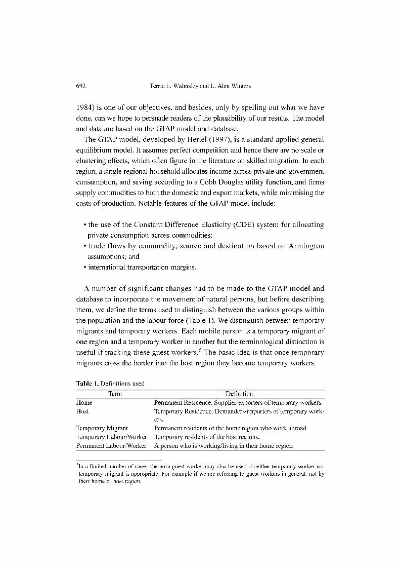
the population and the labour force (Table 1). We distinguish between temporary
migrants and temporary workers. Each mobile person is a temporary migrant of
one region and a temporary worker in another but the terminological distinction is
useful if tracking these guest workers.5 The basic idea is that once temporary
migrants cross the border into the host region they become temporary workers.
5In a limited number of cases, the term guest worker may also be used if neither temporary worker nor
temporary migrant is appropriate. For example if we are referring to guest workers in general, not by
their home or host region.
Table 1. Definitions used
Term Definition
Home Permanent Residence. Supplier/exporters of temporary workers.
Host Temporary Residence. Demanders/importers of temporary work-
ers.
Temporary Migrant Permanent residents of the home region who work abroad.
Temporary Labour/Worker Temporary residents of the host regions.
Permanent Labour/Worker A person who is working/living in their home region
Relaxing the Restrictions on the Temporary Movement of Natural Persons 693
The alterations made to the GTAP model can be divided into six distinct
features: productivity, allocation methods, income, welfare, sectoral allocation and
balancing equations. We refer to the new model as GMig.
A. Productivity
The differences between the productivities of permanent labour and temporary
labour are a significant factor that could potentially affect the expected benefits of
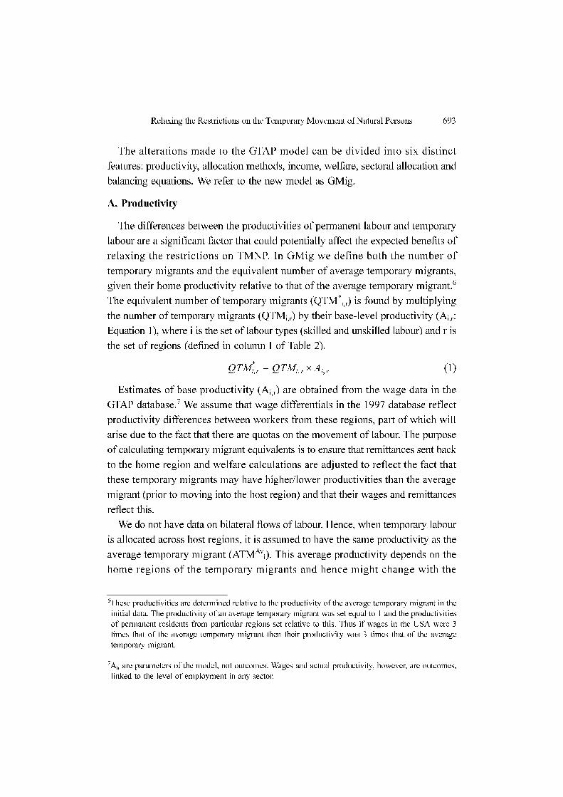
relaxing the restrictions on TMNP. In GMig we define both the number of
temporary migrants and the equivalent number of average temporary migrants,
given their home productivity relative to that of the average temporary migrant.6
The equivalent number of temporary migrants (QTM*i,r) is found by multiplying
the number of temporary migrants (QTMi,r) by their base-level productivity (Ai,r:
Equation 1), where i is the set of labour types (skilled and unskilled labour) and r is
the set of regions (defined in column I of Table 2).
(1)
Estimates of base productivity (Ai,r) are obtained from the wage data in the
GTAP database.7 We assume that wage differentials in the 1997 database reflect
productivity differences between workers from these regions, part of which will
arise due to the fact that there are quotas on the movement of labour. The purpose
of calculating temporary migrant equivalents is to ensure that remittances sent back
to the home region and welfare calculations are adjusted to reflect the fact that
these temporary migrants may have higher/lower productivities than the average
migrant (prior to moving into the host region) and that their wages and remittances
reflect this.
We do not have data on bilateral flows of labour. Hence, when temporary labour
is allocated across host regions, it is assumed to have the same productivity as the
average temporary migrant (ATMAvi). This average productivity depends on the
home regions of the temporary migrants and hence might change with the
QTMi,r
* = QTMi r,
Ai r,×
6These productivities are determined relative to the productivity of the average temporary migrant in the
initial data. The productivity of an average temporary migrant was set equal to 1 and the productivities
of permanent residents from particular regions set relative to this. Thus if wages in the USA were 3
times that of the average temporary migrant then their productivity was 3 times that of the average
temporary migrant.
7Air are parameters of the model, not outcomes. Wages and actual productivity, however, are outcomes,
linked to the level of employment in any sector.
694 Terrie L. Walmsley and L. Alan Winters
composition of temporary flows. For example, if more temporary migrants come
from home regions with lower productivities the average productivity of the
temporary migrant will decline.8 Thus
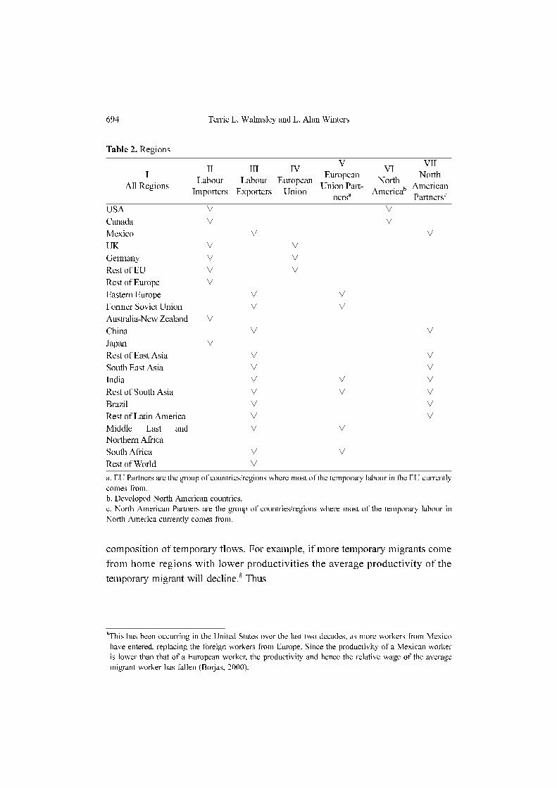
Table 2. Regions
I
All Regions
II
Labour
Importers
III
Labour
Exporters
IV
European
Union
V
European
Union Part-
nersa
VI
North
Americab
VII
North
American
Partnersc
USA ∨ ∨
Canada ∨ ∨
Mexico ∨ ∨
UK ∨ ∨
Germany ∨ ∨
Rest of EU ∨ ∨
Rest of Europe ∨
Eastern Europe ∨ ∨
Former Soviet Union ∨ ∨
Australia-New Zealand ∨
China ∨ ∨
Japan ∨
Rest of East Asia ∨ ∨
South East Asia ∨ ∨
India ∨ ∨ ∨
Rest of South Asia ∨ ∨ ∨
Brazil ∨ ∨
Rest of Latin America ∨ ∨
Middle East and
Northern Africa
∨ ∨
South Africa ∨ ∨
Rest of World ∨
a. EU Partners are the group of countries/regions where most of the temporary labour in the EU currently
comes from.
b. Developed North American countries.
c. North American Partners are the group of countries/regions where most of the temporary labour in
North America currently comes from.
8This has been occurring in the United States over the last two decades, as more workers from Mexico
have entered, replacing the foreign workers from Europe. Since the productivity of a Mexican worker
is lower than that of a European worker, the productivity and hence the relative wage of the average
migrant worker has fallen (Borjas, 2000).
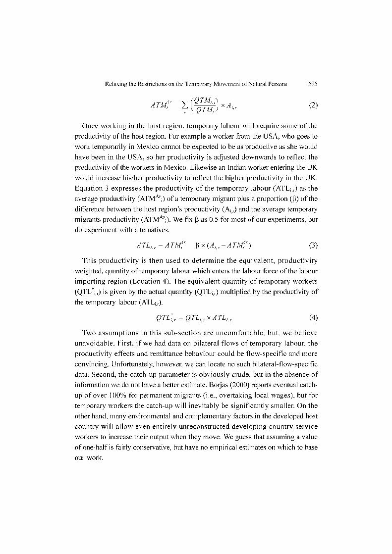
Relaxing the Restrictions on the Temporary Movement of Natural Persons 695
(2)
Once working in the host region, temporary labour will acquire some of the
productivity of the host region. For example a worker from the USA, who goes to
work temporarily in Mexico cannot be expected to be as productive as she would
have been in the USA, so her productivity is adjusted downwards to reflect the
productivity of the workers in Mexico. Likewise an Indian worker entering the UK
would increase his/her productivity to reflect the higher productivity in the UK.
Equation 3 expresses the productivity of the temporary labour (ATLi,r) as the
average productivity (ATMAvi) of a temporary migrant plus a proportion (β) of the
difference between the host region’s productivity (Ai,r) and the average temporary
migrants productivity (ATMAvi). We fix β as 0.5 for most of our experiments, but
do experiment with alternatives.
(3)
This productivity is then used to determine the equivalent, productivity
weighted, quantity of temporary labour which enters the labour force of the labour
importing region (Equation 4). The equivalent quantity of temporary workers
(QTL*i,r) is given by the actual quantity (QTLi,r) multiplied by the productivity of
the temporary labour (ATLi,r).
(4)
Two assumptions in this sub-section are uncomfortable, but, we believe
unavoidable. First, if we had data on bilateral flows of temporary labour, the
productivity effects and remittance behaviour could be flow-specific and more
convincing. Unfortunately, however, we can locate no such bilateral-flow-specific
data. Second, the catch-up parameter is obviously crude, but in the absence of
information we do not have a better estimate. Borjas (2000) reports eventual catch-
up of over 100% for permanent migrants (i.e., overtaking local wages), but for
temporary workers the catch-up will inevitably be significantly smaller. On the
other hand, many environmental and complementary factors in the developed host
country will allow even entirely unreconstructed developing country service
workers to increase their output when they move. We guess that assuming a value
of one-half is fairly conservative, but have no empirical estimates on which to base
our work.
ATMi
Av =
r
∑QTMi r,
QTMi
------------------
⎝ ⎠⎛ ⎞ Ai r,
×
ATLi r, = ATMi
Av + β Ai r,
ATMi
Av–( )×
QTLi r,
* = QTLi r,
ATLi r,×
696 Terrie L. Walmsley and L. Alan Winters
B. Allocation Methods
Since data on bilateral flows of guest workers between regions are generally
unavailable or of dubious quality, the movement of natural persons has been
incorporated into the model in such a way as to minimise the amount of data
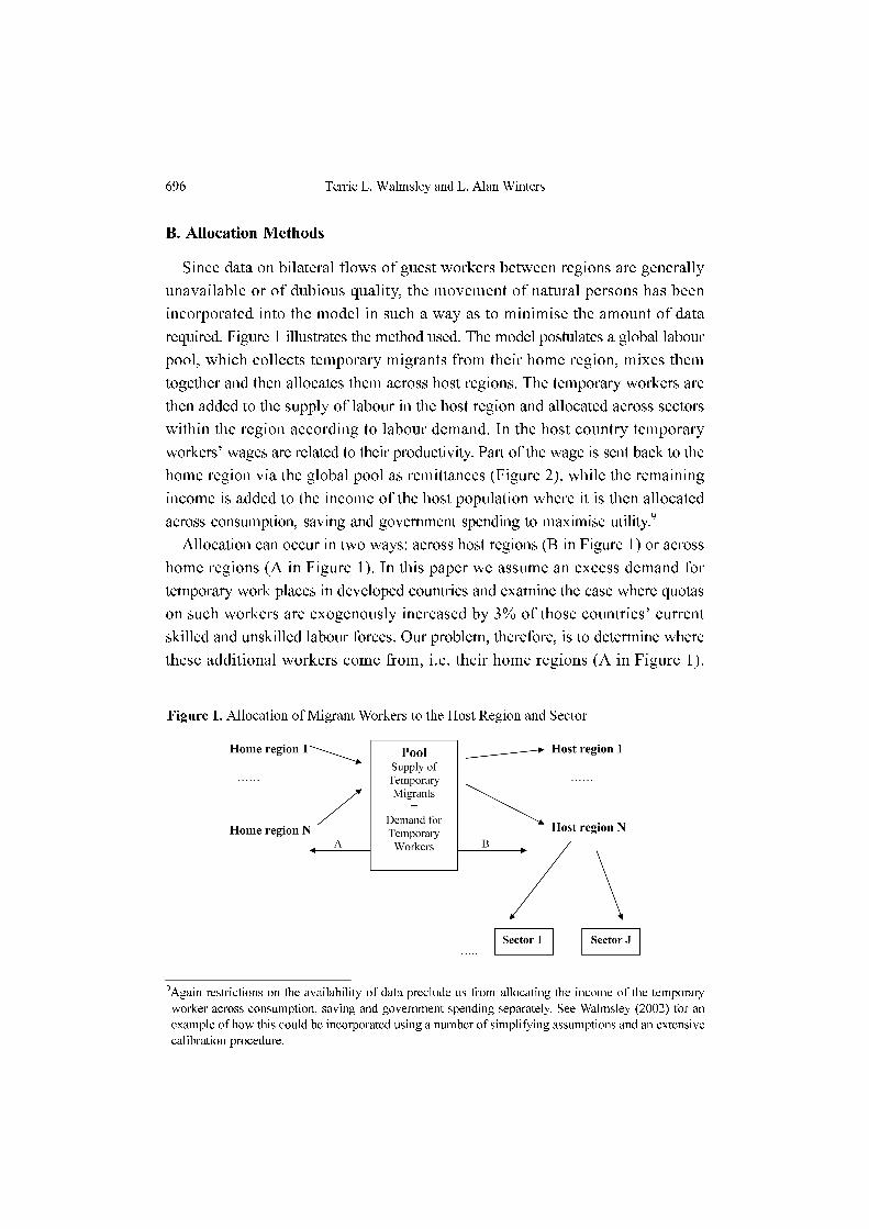
required. Figure 1 illustrates the method used. The model postulates a global labour
pool, which collects temporary migrants from their home region, mixes them
together and then allocates them across host regions. The temporary workers are
then added to the supply of labour in the host region and allocated across sectors
within the region according to labour demand. In the host country temporary
workers’ wages are related to their productivity. Part of the wage is sent back to the
home region via the global pool as remittances (Figure 2), while the remaining
income is added to the income of the host population where it is then allocated
across consumption, saving and government spending to maximise utility.9
Allocation can occur in two ways: across host regions (B in Figure 1) or across
home regions (A in Figure 1). In this paper we assume an excess demand for
temporary work places in developed countries and examine the case where quotas
on such workers are exogenously increased by 3% of those countries’ current
skilled and unskilled labour forces. Our problem, therefore, is to determine where
these additional workers come from, i.e. their home regions (A in Figure 1).
9Again restrictions on the availability of data preclude us from allocating the income of the temporary
worker across consumption, saving and government spending separately. See Walmsley (2002) for an
example of how this could be incorporated using a number of simplifying assumptions and an extensive
calibration procedure.
Figure 1. Allocation of Migrant Workers to the Host Region and Sector
Relaxing the Restrictions on the Temporary Movement of Natural Persons 697
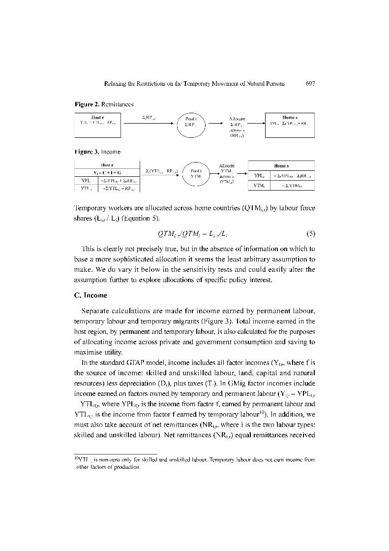
Temporary workers are allocated across home countries (QTMi,r) by labour force
shares (Li,r / Li) (Equation 5).
(5)
This is clearly not precisely true, but in the absence of information on which to
base a more sophisticated allocation it seems the least arbitrary assumption to
make. We do vary it below in the sensitivity tests and could easily alter the
assumption further to explore allocations of specific policy interest.
C. Income
Separate calculations are made for income earned by permanent labour,
temporary labour and temporary migrants (Figure 3). Total income earned in the
host region, by permanent and temporary labour, is also calculated for the purposes
of allocating income across private and government consumption and saving to
maximise utility.
In the standard GTAP model, income includes all factor incomes (Yf,r, where f is
the source of income: skilled and unskilled labour, land, capital and natural
resources) less depreciation (Dr), plus taxes (Tr). In GMig factor incomes include
income earned on factors owned by temporary and permanent labour (Yf,r = YPLf,r
+ YTLf,r, where YPLf,r is the income from factor f, earned by permanent labour and
YTLf,r is the income from factor f earned by temporary labour10). In addition, we
must also take account of net remittances (NRi,r, where i is the two labour types:
skilled and unskilled labour). Net remittances (NRi,r) equal remittances received
QTMi r,
/QTMi = L
i r,/L
i
Figure 2. Remittances
Figure 3. Income
10YTLf,r is non-zero only for skilled and unskilled labour. Temporary labour does not earn income from
other factors of production.
698 Terrie L. Walmsley and L. Alan Winters
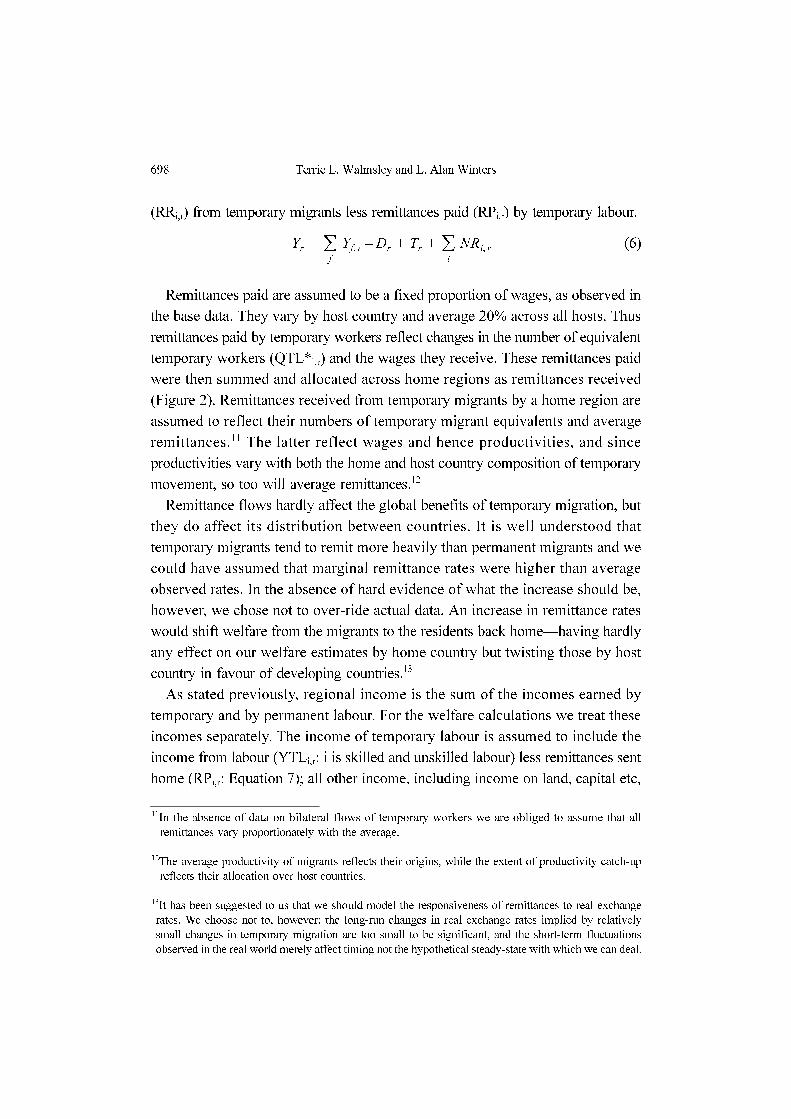
(RRi,r) from temporary migrants less remittances paid (RPi,r) by temporary labour.
(6)
Remittances paid are assumed to be a fixed proportion of wages, as observed in
the base data. They vary by host country and average 20% across all hosts. Thus
remittances paid by temporary workers reflect changes in the number of equivalent
temporary workers (QTL*i,r) and the wages they receive. These remittances paid
were then summed and allocated across home regions as remittances received
(Figure 2). Remittances received from temporary migrants by a home region are
assumed to reflect their numbers of temporary migrant equivalents and average
remittances.11 The latter reflect wages and hence productivities, and since
productivities vary with both the home and host country composition of temporary
movement, so too will average remittances.12
Remittance flows hardly affect the global benefits of temporary migration, but
they do affect its distribution between countries. It is well understood that
temporary migrants tend to remit more heavily than permanent migrants and we
could have assumed that marginal remittance rates were higher than average
observed rates. In the absence of hard evidence of what the increase should be,
however, we chose not to over-ride actual data. An increase in remittance rates
would shift welfare from the migrants to the residents back home—having hardly
any effect on our welfare estimates by home country but twisting those by host
country in favour of developing countries.13
As stated previously, regional income is the sum of the incomes earned by
temporary and by permanent labour. For the welfare calculations we treat these
incomes separately. The income of temporary labour is assumed to include the
income from labour (YTLi,r: i is skilled and unskilled labour) less remittances sent
home (RPi,r: Equation 7); all other income, including income on land, capital etc,
Yr =
f
∑ Yf r,Dr– + Tr +
i
∑ NRi r,
11In the absence of data on bilateral flows of temporary workers we are obliged to assume that all
remittances vary proportionately with the average.
12The average productivity of migrants reflects their origins, while the extent of productivity catch-up
reflects their allocation over host countries.
13It has been suggested to us that we should model the responsiveness of remittances to real exchange
rates. We choose not to, however: the long-run changes in real exchange rates implied by relatively
small changes in temporary migration are too small to be significant, and the short-term fluctuations
observed in the real world merely affect timing not the hypothetical steady-state with which we can deal.
Relaxing the Restrictions on the Temporary Movement of Natural Persons 699
taxes and remittances received are earned by permanent labour.
(7)
The income of temporary migrants by home region is discussed in section 2.4 as
part of the calculation of welfare of temporary migrants.
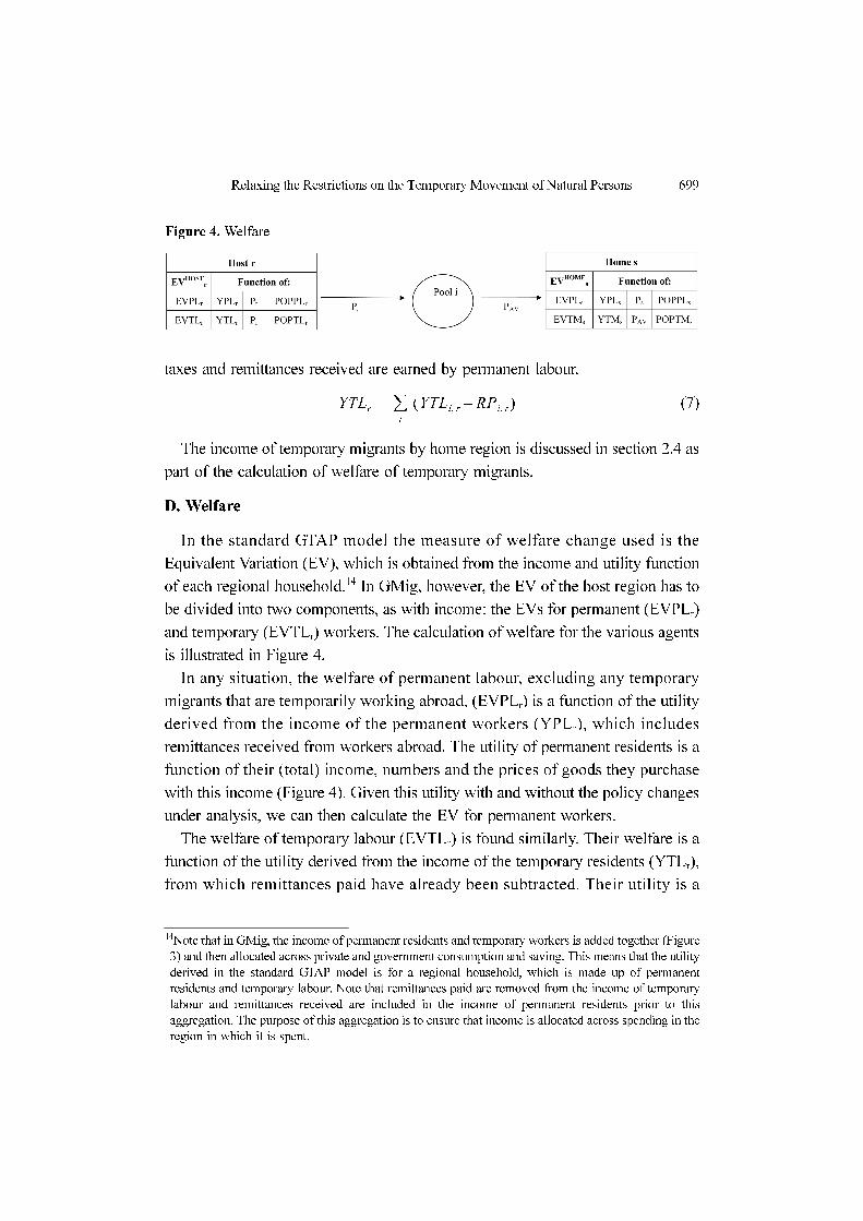
D. Welfare
In the standard GTAP model the measure of welfare change used is the
Equivalent Variation (EV), which is obtained from the income and utility function
of each regional household.14 In GMig, however, the EV of the host region has to
be divided into two components, as with income: the EVs for permanent (EVPLr)
and temporary (EVTLr) workers. The calculation of welfare for the various agents
is illustrated in Figure 4.
In any situation, the welfare of permanent labour, excluding any temporary
migrants that are temporarily working abroad, (EVPLr) is a function of the utility
derived from the income of the permanent workers (YPLr), which includes
remittances received from workers abroad. The utility of permanent residents is a
function of their (total) income, numbers and the prices of goods they purchase
with this income (Figure 4). Given this utility with and without the policy changes
under analysis, we can then calculate the EV for permanent workers.
The welfare of temporary labour (EVTLr) is found similarly. Their welfare is a
function of the utility derived from the income of the temporary residents (YTLr),
from which remittances paid have already been subtracted. Their utility is a
YTLr =
f
∑ YTLi r,RPi r,
–( )
14Note that in GMig, the income of permanent residents and temporary workers is added together (Figure
3) and then allocated across private and government consumption and saving. This means that the utility
derived in the standard GTAP model is for a regional household, which is made up of permanent
residents and temporary labour. Note that remittances paid are removed from the income of temporary
labour and remittances received are included in the income of permanent residents prior to this
aggregation. The purpose of this aggregation is to ensure that income is allocated across spending in the
region in which it is spent.
Figure 4. Welfare
700 Terrie L. Walmsley and L. Alan Winters
function of their (total) income, numbers and the price level in the host region
(Figure 4), and from these EVs can be calculated.
The welfare change for a region as host ( ), can now be found by
summing the parts for permanent and temporary labour (Figure 4). The total EV of
all temporary workers (EVTL) is then equal to the sum across regions of the EVs
of all the temporary workers (EVTLr, Equation 9).
(8)
(9)
The income of the temporary labour by host region and labour type is
aggregated across host regions (Equation 10) and distributed across home regions
to find the income attributable to temporary migrants from each region (Equation
11: Figure 3). The distribution of total income by all temporary labour (YTMi)
across home regions depends on the equivalent quantities of temporary migrants
(QTM*i,r) from the home region relative to the total (QTM*i).
(10)
(11)
This income is then used to determine the utility and EV of the temporary
migrants (Figure 4). An average price has to be used to determine utility of
temporary migrants - the average price for goods paid by temporary labour in their
host regions.15
Once the EV of temporary migrants is determined, the welfare change by home
region ( , Equation 12), regardless of temporary residence (Figure 4), and
the world welfare change (WEV, Equation 13) can also be calculated by simply
summing the relevant regional figures.
(12)
(13)
EVr
HOST
EVr
HOST = EVPLr + EVTLr
EVTL =
r
∑ EVTLr
YTMi =
r
∑ YTLi r,RPi r,
–( )
YTMr = QTMt r,
*
QTMi
*------------------ YTMi×
EVr
HOME
EVr
HOME = EVTMr + EVPLr
WEV =
r
∑ EVr
home =
r
∑ EVr
host
15Another method would have been to aggregate the EV of all temporary labour across host regions and
then allocate this welfare across home regions according to the shares. This would have avoided the
need to determine an average price. However this method would not have allowed us to take into
account differences in the supply of skilled and unskilled labour across home regions.
Relaxing the Restrictions on the Temporary Movement of Natural Persons 701
E. Sectoral Allocation
The last issue to be examined relates to what industries the temporary labour
will be employed in or what sectors the temporary migrants will come from. In the
standard GTAP model, labour moves across sectors to equalise the wage - thus
labour moves to the sectors with the highest demand. This is also the standard
closure for GMig. On the other hand, since Mode 4 is restricted to services and
since particular service sectors in the developed economies, e.g. the computing
sector in the USA, are interested in obtaining skilled temporary workers, it is
interesting to think what happens if labour is restricted to specific sectors.
This is achieved in the model by dividing the sectors into two groups: one group
of sectors which employ temporary labour (A); and a second group of sectors
which do not (B). The supply of labour to each group must equal its demand, and
labour can flow freely within each group but not between them. All temporary
labour flows are supplied to the group of sectors which accept temporary labour
(A), while the supply of labour to the other group (B) is held fixed. This approach
also has implications for permanent labour. In order that the inflow of temporary
labour not just be off-set by outflows of permanent labour, we have to fix supplies
of permanent labour in each group. Hence labour is not perfectly mobile, except
between sectors of the same group, and wages differ between the two groups. We
note that Borjas and Freeman (1992) found that permanent residents do tend, in
fact, to move out of geographical areas in which there has been an influx of foreign
workers, leaving the total labour force unchanged, so our assumption of the
opposite for TMNP should be considered rather carefully.
F. Balancing Equation
Finally, in all our exercises the total number of temporary migrants (QTMi) from
all home regions equals the total number of temporary labour (QTLi) in all host
regions.16
(14)
III. Data
The primary database used to support the GMig model is version 5 of the GTAP
QTMi = QTL
i
16The share allocation method ensures this equality holds, although other methods may not.
702 Terrie L. Walmsley and L. Alan Winters
Database (Dimaranan et al., 2001). Version 5 of the GTAP database contains 66
countries/regions and 57 sectors. The GTAP database was supplemented with
additional data on the labour force, numbers of temporary migrants and workers,
and their remittances and wages. In this section we provide the sources for this
additional data, outlining the assumptions made for filling in any missing data, the
calculation of wage data and the calibration procedure used.
The additional data were collected at the country level for 211 countries and
then aggregated into the 66 regions identified in version 5 of the GTAP database.
The new data include information on population, labour force, numbers of skilled
and unskilled labour, the number of temporary workers by skill level located in
each region, the number of temporary migrants by skill level from each region and
the value of remittances entering and leaving the region. Data were found for as
many countries as possible, using the International Labour Organisation’s
International Labour Migration Database,17 and missing values were then filled to
get estimates for all 211 countries.
The filling process involved using data on the numbers of temporary migrants
and of temporary labour to estimate remittances in and out respectively or
alternatively using remittance data to obtain estimates of numbers of temporary
migrants and/or labour. Where data on neither remittances nor the number of
people were available, the values were assumed be zero. This was the case for
temporary migrants from the United States, Canada, UK and Germany and for
temporary labour working in Mexico.
In a limited number of cases the ILO International Migration database also
included estimates of the skill level of the temporary labour. These estimates were
used wherever possible to obtain a split between skilled and unskilled workers. In
the other regions, the skill levels of migrants were assumed to reflect those of their
home labour force, while the skill levels of temporary workers were assumed to
reflect the overall skill breakdown of the temporary migrants.
Once the numbers of workers were obtained, these were used to find the wages
earned by the temporary workers. A measure of the productivity of a worker,
relative to the average migrant worker was estimated based on the wage per
17A handful of these numbers were altered if other evidence suggested that the number provided by the
ILO International Migration Database was a significant underestimate. For example the number of
temporary migrants from the Philippines and the number of temporary workers in the USA were revised
upwards to reflect other data collected by Walmsley (1999). The revisions to temporary workers in the
USA reflect estimates of the number of illegal temporary workers in the USA.
Relaxing the Restrictions on the Temporary Movement of Natural Persons 703
worker in each region. A temporary worker entering the host region was assumed
to have the average wage of a temporary migrant plus a portion of the difference
between the average wage of a temporary migrant and the wage obtained by a
permanent resident of the host region (Related to Equation 3). This reflects the fact
that the temporary worker’s productivity will partially adjust to reflect the
productivity in the host region. For example, the productivity of an African
entering the UK will increase relative to his productivity at home as he/she will
now have more productive tools. However, it will not increase to the same level as
a permanent resident as foreigners do not have all the specific tools required for the
UK, e.g. language, UK education etc. Borjas (2000) examined the case of
permanent migrants entering the USA and found that they received 80-90% of the
wages of a permanent resident initially.18 This proportion increases as the migrant’s
time in the country increases and additional USA specific skills were gathered.19
As our workers are temporary, they do not have time to adapt and a temporary
migrant is unlikely to have the same entrepreneurial characteristics as a permanent
migrant. Hence we expect that temporary migrants would have a smaller degree of
convergence to the permanent residents’ wage. In this paper we generally assume
that temporary labour acquires 50% of the difference in productivities, but we also
experiment with values of 25% and 75% (Equation 3).
Remittances are an important source of income for many labour exporting
regions, such as Thailand and the Philippines. The inclusion of remittances in the
income of the region means that income is now defined as income earned on land,
labour and capital located in the region plus taxes plus net remittances received.
The GTAP database (which ignores remittances) must be altered to reflect this new
definition and to ensure that this new definition of income is consistent with
aggregate spending.
To ensure that income equals spending in GMig, one of the GTAP components
of spending must be altered. We choose to reduce saving by the value of the net
18Whether the average migrant received 80% or 90% depends on the skills of the migrant worker. In the
1970s migrants to the USA earned 90% of the wage of a USA worker, as many of them were from
Europe and had higher skills. More recently, with the increase in immigrants from Latin America, skills
and hence wages, have declined.
19In fact Borjas (2000) found that as time progressed migrants’ wages increased to 10% more than the
average native wage. He suggested that this may be the result of self-selection, i.e. a migrant who
chooses to move permanently may be more entrepreneurial than the average worker in his/her home
country.
704 Terrie L. Walmsley and L. Alan Winters
remittances paid, because:
• In the construction of the GTAP database, Private Consumption and
Government consumption are adjusted to ensure that they are consistent with
other sources, such as World Bank. Therefore in the GTAP database, it is
saving which adjusts to take account of the fact that GTAP takes no account of
remittances. Hence if we wish to include remittances, saving should be
adjusted back again.
• The use of saving minimises the re-calibration required. The only restriction
pertaining to saving in the GTAP database is that global saving equals global
investment. Since global remittances received equal global remittances paid,
the global saving – investment identity is automatically satisfied when these
remittances are added to or subtracted from saving.
Finally the data were aggregated into 21 regions and 22 sectors for undertaking
the analysis. A list of the regions and the commodities can be found in column I of
Table 2 and the stub of Figure 3, respectively.
IV. Simulations
A number of simulations were undertaken using the GMig model to examine
how relaxing the restrictions on the temporary movement of natural persons
(TMNP) is likely to affect developed and developing countries. The paper
commences by focusing on a single simulation of an increase in developed country
quotas on the numbers of skilled and unskilled temporary workers. Following this
the effects of other issues, such as sectoral allocation, the size of the shock and the
choice of labour importing and exporting regions, are examined.
Quotas on the temporary movement of natural persons are assumed to increase
in a number of traditionally labour importing regions, and to be filled by labour
from a number of traditionally labour exporting countries according to their labour
force shares. Table 2 divides the regions used in this analysis in to labour importing
and labour exporting regions (columns II and III respectively).20 The quotas are
increased by an amount which would allow the quantity of both skilled and
20The decision of whether a region was a labour exporter or importer was based on wage rates (high
wages were expected in labour importing countries and low wages in labour exporters), data on the
quantities of temporary migrants relative to temporary workers and the level of development.
Relaxing the Restrictions on the Temporary Movement of Natural Persons 705
unskilled labour supplied in the host (or labour importing) countries to increase by
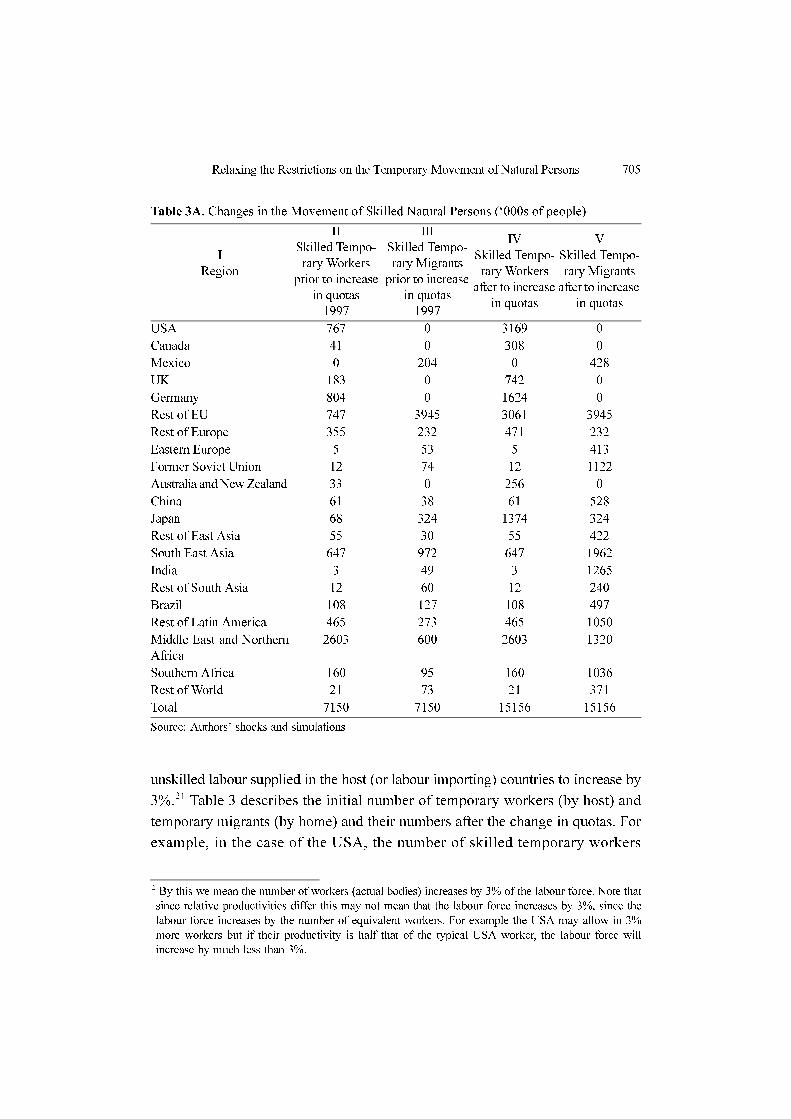
3%.21 Table 3 describes the initial number of temporary workers (by host) and
temporary migrants (by home) and their numbers after the change in quotas. For
example, in the case of the USA, the number of skilled temporary workers
21By this we mean the number of workers (actual bodies) increases by 3% of the labour force. Note that
since relative productivities differ this may not mean that the labour force increases by 3%, since the
labour force increases by the number of equivalent workers. For example the USA may allow in 3%
more workers but if their productivity is half that of the typical USA worker, the labour force will
increase by much less than 3%.
Table 3A. Changes in the Movement of Skilled Natural Persons (‘000s of people)
I
Region
II
Skilled Tempo-
rary Workers
prior to increase
in quotas
1997
III
Skilled Tempo-
rary Migrants
prior to increase
in quotas
1997
IV
Skilled Tempo-
rary Workers
after to increase
in quotas
V
Skilled Tempo-
rary Migrants
after to increase
in quotas
USA 767 0 3169 0
Canada 41 0 308 0
Mexico 0 204 0 428
UK 183 0 742 0
Germany 804 0 1624 0
Rest of EU 747 3945 3061 3945
Rest of Europe 355 232 471 232
Eastern Europe 5 53 5 413
Former Soviet Union 12 74 12 1122
Australia and New Zealand 33 0 256 0
China 61 38 61 528
Japan 68 324 1374 324
Rest of East Asia 55 30 55 422
South East Asia 647 972 647 1962
India 3 49 3 1265
Rest of South Asia 12 60 12 240
Brazil 108 127 108 497
Rest of Latin America 465 273 465 1050
Middle East and Northern
Africa
2603 600 2603 1320
Southern Africa 160 95 160 1036
Rest of World 21 73 21 371
Total 7150 7150 15156 15156
Source: Authors’ shocks and simulations
706 Terrie L. Walmsley and L. Alan Winters
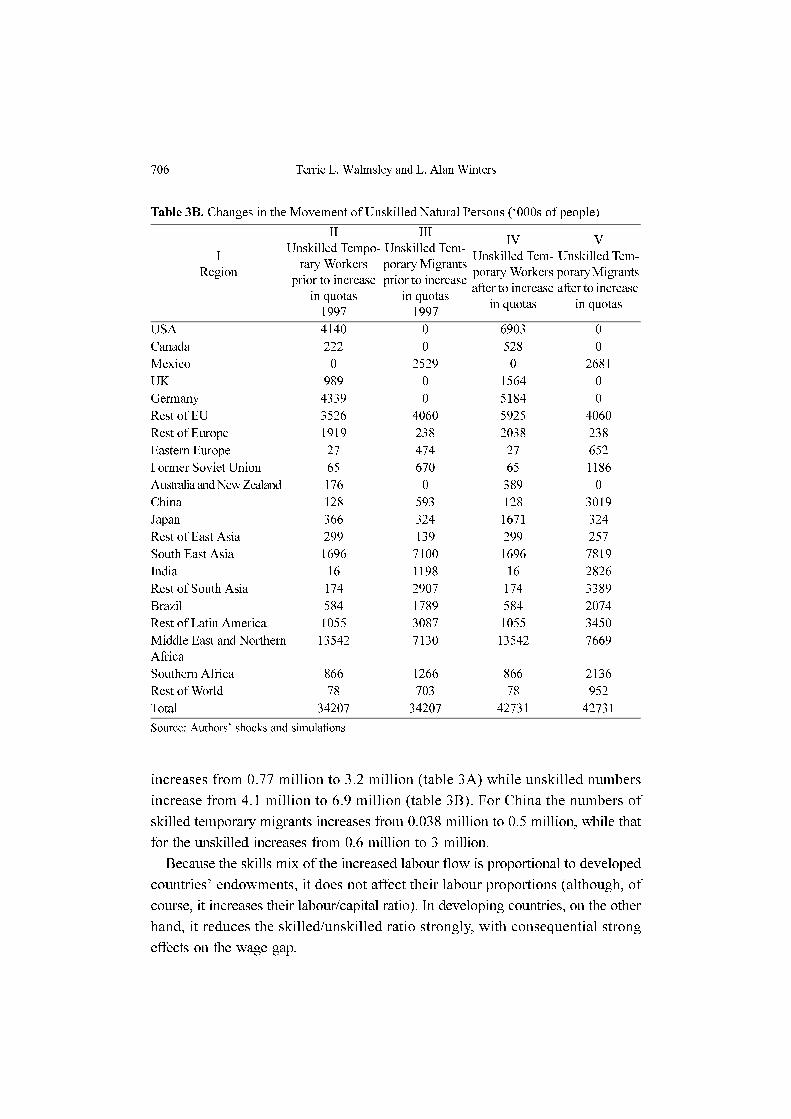
increases from 0.77 million to 3.2 million (table 3A) while unskilled numbers
increase from 4.1 million to 6.9 million (table 3B). For China the numbers of
skilled temporary migrants increases from 0.038 million to 0.5 million, while that
for the unskilled increases from 0.6 million to 3 million.
Because the skills mix of the increased labour flow is proportional to developed
countries’ endowments, it does not affect their labour proportions (although, of
course, it increases their labour/capital ratio). In developing countries, on the other
hand, it reduces the skilled/unskilled ratio strongly, with consequential strong
effects on the wage gap.
Table 3B. Changes in the Movement of Unskilled Natural Persons (‘000s of people)
I
Region
II
Unskilled Tempo-
rary Workers
prior to increase
in quotas
1997
III
Unskilled Tem-
porary Migrants
prior to increase
in quotas
1997
IV
Unskilled Tem-
porary Workers
after to increase
in quotas
V
Unskilled Tem-
porary Migrants
after to increase
in quotas
USA 4140 0 6903 0
Canada 222 0 528 0
Mexico 0 2529 0 2681
UK 989 0 1564 0
Germany 4339 0 5184 0
Rest of EU 3526 4060 5925 4060
Rest of Europe 1919 238 2038 238
Eastern Europe 27 474 27 652
Former Soviet Union 65 670 65 1186
Australia and New Zealand 176 0 389 0
China 128 593 128 3019
Japan 366 324 1671 324
Rest of East Asia 299 139 299 257
South East Asia 1696 7100 1696 7819
India 16 1198 16 2826
Rest of South Asia 174 2907 174 3389
Brazil 584 1789 584 2074
Rest of Latin America 1055 3087 1055 3450
Middle East and Northern
Africa
13542 7130 13542 7669
Southern Africa 866 1266 866 2136
Rest of World 78 703 78 952
Total 34207 34207 42731 42731
Source: Authors’ shocks and simulations
Relaxing the Restrictions on the Temporary Movement of Natural Persons 707
V. The Results
A. Macroeconomic Effects
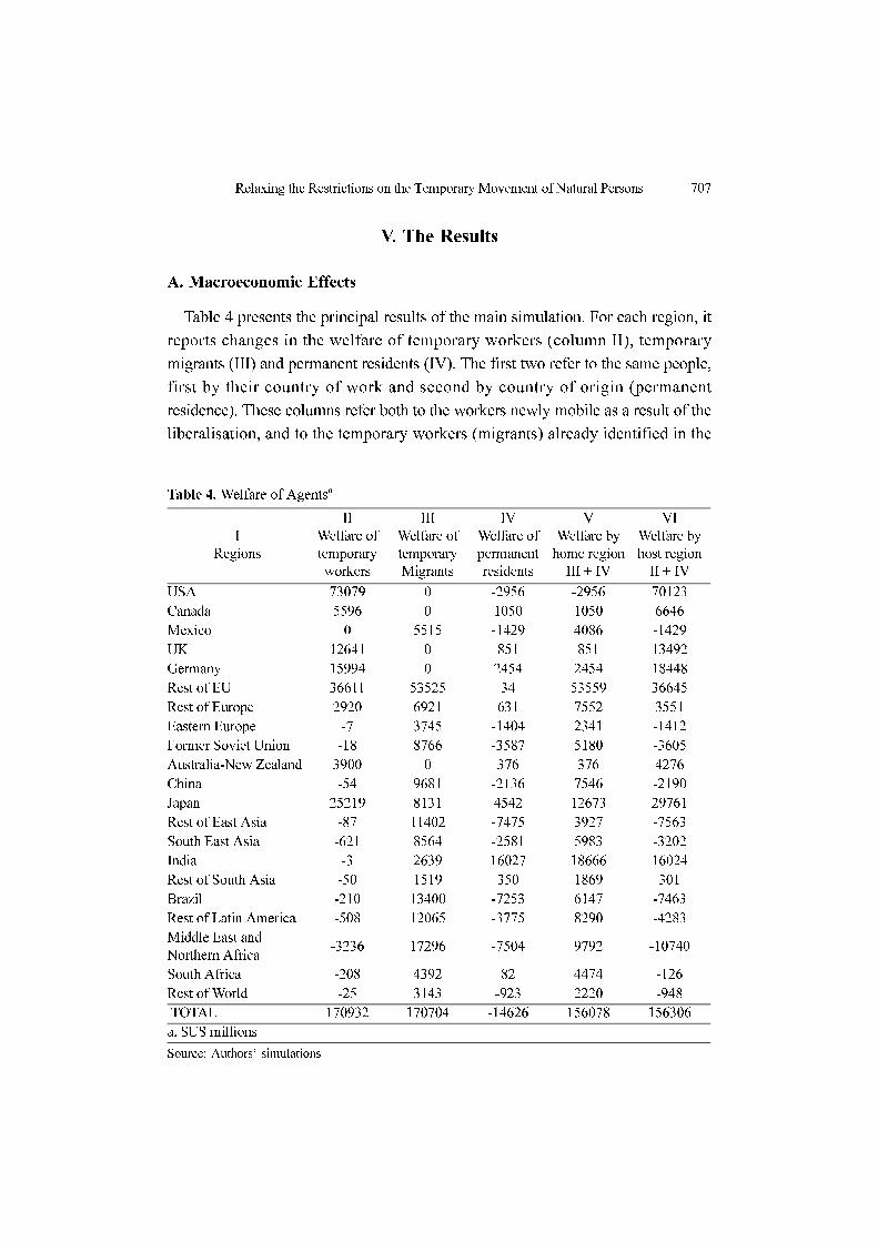
Table 4 presents the principal results of the main simulation. For each region, it
reports changes in the welfare of temporary workers (column II), temporary
migrants (III) and permanent residents (IV). The first two refer to the same people,
first by their country of work and second by country of origin (permanent
residence). These columns refer both to the workers newly mobile as a result of the
liberalisation, and to the temporary workers (migrants) already identified in the
Table 4. Welfare of Agentsa
I
Regions
II
Welfare of
temporary
workers
III
Welfare of
temporary
Migrants
IV
Welfare of
permanent
residents
V
Welfare by
home region
III + IV
VI
Welfare by
host region
II + IV
USA 73079 0 -2956 -2956 70123
Canada 5596 0 1050 1050 6646
Mexico 0 5515 -1429 4086 -1429
UK 12641 0 851 851 13492
Germany 15994 0 2454 2454 18448
Rest of EU 36611 53525 34 53559 36645
Rest of Europe 2920 6921 631 7552 3551
Eastern Europe -7 3745 -1404 2341 -1412
Former Soviet Union -18 8766 -3587 5180 -3605
Australia-New Zealand 3900 0 376 376 4276
China -54 9681 -2136 7546 -2190
Japan 25219 8131 4542 12673 29761
Rest of East Asia -87 11402 -7475 3927 -7563
South East Asia -621 8564 -2581 5983 -3202
India -3 2639 16027 18666 16024
Rest of South Asia -50 1519 350 1869 301
Brazil -210 13400 -7253 6147 -7463
Rest of Latin America -508 12065 -3775 8290 -4283
Middle East and
Northern Africa-3236 17296 -7504 9792 -10740
South Africa -208 4392 82 4474 -126
Rest of World -25 3143 -923 2220 -948
TOTAL 170932 170704 -14626 156078 156306
a. $US millions
Source: Authors’ simulations
708 Terrie L. Walmsley and L. Alan Winters
base run. The table also presents the results for each region as a “home” country
(V) - permanent residents plus temporary migrants (in SNA terms a
“national”concept) - and “host” country - permanent resident plus temporary
workers (a “domestic” concept).
The increase in the developed countries’ quotas of both skilled and unskilled
temporary labour increases world welfare by an estimated $US156 billion – about
0.6% of initial income. The gain, which arises from increasing quotas by only 3%
of the labour force of the developed economies, is considerable, and is around 1.5
times that expected from the liberalisation of all remaining trade restrictions
($US104 billion).
The labour exporting (or developing) economies gain most from the increase in
quotas on the movement of labour (Column V in Table 4). Most of this increase is
the result of higher incomes earned by the temporary migrants themselves (Column
III). Despite the higher remittances received from temporary workers, the
permanent residents of the developing countries generally lose as a result of the
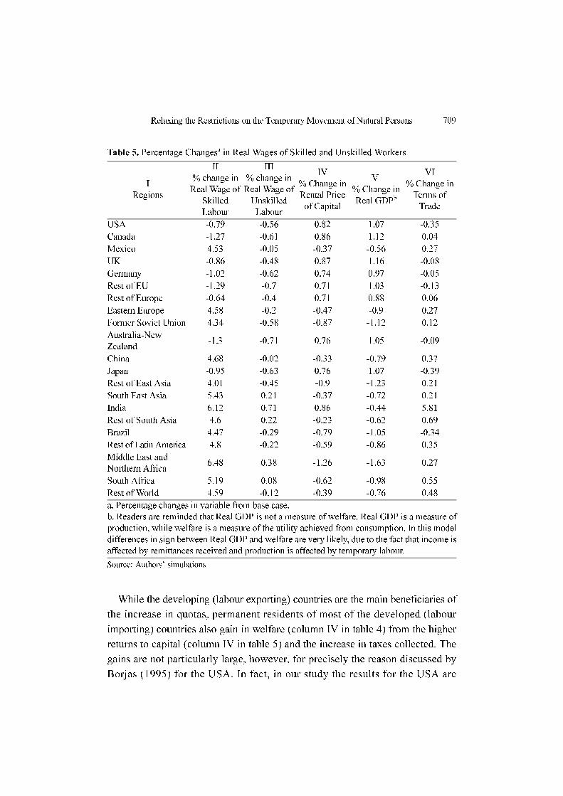
outflow of temporary migrants (Column IV): the decrease in labour endowments
dramatically raises the wages of skilled workers (Column II of Table 5), but has
mixed effects on unskilled wages (Column III). Real GDP (Column V) and the
returns to other factors such as capital (Column IV) fall. In the few cases in which
the income and welfare of permanent residents rise, India, the rest of South Asia
and South Africa, they do so because increased remittances outweigh the declines
in capital income. In India, remittances increase strongly by 4% of the initial level
of income. This increases the demand for domestic goods because India is
relatively closed, reduces the decline in production in the economy, and raises local
prices, which, in turn, generates a large terms of trade gain. Real wages for both
skilled and unskilled workers rise22 (Columns II and III in Table 5). With the
exception of Brazil, developing economies experience an improvement in their
terms of trade (Column VI): shifting factors from developing to developed
countries reduces the relative supply of developing country output and hence raises
its price relative to that of the developed countries.
22There may be a case for modelling India to have a pool of unemployed unskilled workers who will
become employed in India as a result of the outflow of temporary migrants. While in this case the
quantity of unskilled workers would rise, the real wages of unskilled workers would remain fixed. Total
earnings would rise as there would be fewer people in the informal or unproductive sectors and so the
overall welfare effect would not be very different from that reported with flexible wages. This is
examined in section 5.7.
Relaxing the Restrictions on the Temporary Movement of Natural Persons 709
While the developing (labour exporting) countries are the main beneficiaries of
the increase in quotas, permanent residents of most of the developed (labour
importing) countries also gain in welfare (column IV in table 4) from the higher
returns to capital (column IV in table 5) and the increase in taxes collected. The
gains are not particularly large, however, for precisely the reason discussed by
Borjas (1995) for the USA. In fact, in our study the results for the USA are
Table 5. Percentage Changesa in Real Wages of Skilled and Unskilled Workers
I
Regions
II
% change in
Real Wage of
Skilled
Labour
III
% change in
Real Wage of
Unskilled
Labour
IV
% Change in
Rental Price
of Capital
V
% Change in
Real GDPb
VI
% Change in
Terms of
Trade
USA -0.79 -0.56 0.82 1.07 -0.35
Canada -1.27 -0.61 0.86 1.12 0.04
Mexico 4.53 -0.05 -0.37 -0.56 0.27
UK -0.86 -0.48 0.87 1.16 -0.08
Germany -1.02 -0.62 0.74 0.97 -0.05
Rest of EU -1.29 -0.7 0.71 1.03 -0.13
Rest of Europe -0.64 -0.4 0.71 0.88 0.06
Eastern Europe 4.58 -0.2 -0.47 -0.9 0.27
Former Soviet Union 4.34 -0.58 -0.87 -1.12 0.12
Australia-New
Zealand-1.3 -0.71 0.76 1.05 -0.09
China 4.68 -0.02 -0.33 -0.79 0.37
Japan -0.95 -0.63 0.76 1.07 -0.39
Rest of East Asia 4.01 -0.45 -0.9 -1.23 0.21
South East Asia 5.43 0.21 -0.37 -0.72 0.21
India 6.12 0.71 0.86 -0.44 5.81
Rest of South Asia 4.6 0.22 -0.23 -0.62 0.69
Brazil 4.47 -0.29 -0.79 -1.05 -0.34
Rest of Latin America 4.8 -0.22 -0.59 -0.86 0.35
Middle East and
Northern Africa6.48 0.38 -1.26 -1.63 0.27
South Africa 5.19 0.08 -0.62 -0.98 0.55
Rest of World 4.59 -0.12 -0.39 -0.76 0.48
a. Percentage changes in variable from base case.
b. Readers are reminded that Real GDP is not a measure of welfare. Real GDP is a measure of
production, while welfare is a measure of the utility achieved from consumption. In this model
differences in sign between Real GDP and welfare are very likely, due to the fact that income is
affected by remittances received and production is affected by temporary labour.
Source: Authors’ simulations
710 Terrie L. Walmsley and L. Alan Winters
contaminated by data failures which make them absurd.23 Real GDP increases
substantially in all of the labour importing (developed) economies (Column V in
Table 5) as a result of the increase in skilled and unskilled labour endowments, and
in most cases the terms of trade decline, as the output of local varieties grows. The
terms of trade decline is the same effect as Davis and Weinstein (2002) use to
argue that factor mobility is harmful to developed countries. They assumed
equiproportionate increases in all factors, so that the (negative) size effect was all
that remained, whereas we have changes in developed countries’ factor mixes.24
One number of note in table 4 is the strong positive effects on developed
countries’ temporary migrants – i.e. those who leave a developed country to work
abroad. This reflects the fact that over half of the stock of skilled temporary
migrants identified in our database comes from the ‘Rest of the EU’ region (EU
less than UK and Germany). The distribution of total welfare of temporary workers
across temporary migrants is made on the assumption that all temporary migrants
are mobile and can fill the new jobs created by increasing quotas in the labour
importing regions. This includes the temporary migrants from ‘Rest of EU’. Even
though wages in the labour importing regions fall as a result of the inflow of
labour, the average wages of temporary workers rise strongly. This is because the
increase in quotas is restricted to developed economies, where wages are higher, so
that the mix of the world’s supply of temporary jobs becomes much more
favourable, and, as a result, welfare increases strongly for temporary migrants as a
group.25 Given our unavoidable assumption of a global pool of temporary workers,
the benefits of this gain are distributed to all regions which report some temporary
migrants.
23There is no tax information for the USA economy in the GTAP data base, reflecting the fact that no tax
information was provided in the initial IO table. As a result net indirect taxes reflect only subsidies and
the increase in output increases subsidies and hence distortion. If data on taxes were available, welfare
would increase in the USA, as it has in the other developed economies. Assuming taxes of 4% on
private consumption and 1.5% on output (based on tax rates in other developed countries) and adjusting
other US data compatibly, the USA gains $1.61 billion in the exercise above.
24Related to terms-of-trade changes, but not reported are real exchange rate changes as temporary labour
flows affect the relative prices of traded and non-traded goods.
25Of the initial temporary jobs, 7.1 million are skilled, of which 3 million (42%) are in developed
countries; and 34.2 million unskilled, with 1.6 million (45.8%) in developed countries. Our assumed
quota increases the developed country shares of temporary jobs to 73% and 57% respectively. At initial
wage levels the changes in the composition of these jobs raises the average skilled temporary worker
wage from 10.9 to 11.4 and from 7.8 to 8.8 for unskilled workers.
Relaxing the Restrictions on the Temporary Movement of Natural Persons 711
At first blush the assumption that all temporary migrants are mobile and can
move to fill the new quotas in the labour importing regions seems strange, but in
fact is not at all unreasonable. Although the jobs that migrants do are quasi-
permanent, migration is temporary, and the stock of temporary workers is constantly
turning over. Even if the same individuals were involved through time they would
be obliged to circulate among host countries.26
Finally, the increase in the rental price of capital raises the current rate of return -
defined as the rental price relative to the cost of capital net of depreciation. The
high current rate of return leads to higher levels of investment in the developed
economies, which increases final demand in proportion to the base-year investment
vector.27
B. Sectoral Output
Figures 3 and 4 illustrate the effect of the increase in quotas on domestic
production in a selection of labour importing and labour exporting regions.
Agriculture is the least affected of all the sectors in both the developed and
developing economies. Private consumption of agriculture has a low income
elasticity of demand, there is little intermediate demand from other sectors, and
agriculture is very land intensive in developing countries and capital intensive in
developed countries. Conversely, the skilled labour intensive sectors experience the
largest shocks. In the developed economies, services, particularly trade, business
services and other services, and most of the manufacturing sectors are positively
affected, while in developing (labour exporting) countries the opposite is true.
India, again, shows a slightly different pattern, with production in some services
and agricultural sectors increasing. These sectors benefit from the additional
income received as remittances: a high proportion (approximately 97%) of their
output is supplied to the domestic market, and, with the exception of construction,
these sectors are very capital or land intensive, rather than labour intensive. In the
case of construction, the increase in output is primarily due to an increase in
26An alternative assumption in which the initial temporary jobs in the database are presumed not to
change the nationality of their incumbents, and thus in which temporary migrants from developed areas
are not eligible to take up the new positions in the developed economies would lead to a different
distribution of welfare gains. It involves lower gains for developed countries and higher gains for
developing countries, and is discussed in more detail in Appendix 1.
27In the long run, higher investment will reduce rates of return and increase output, but in our static model
only the final demand element is modelled.
712 Terrie L. Walmsley and L. Alan Winters
investment resulting from an increase in the return to capital.
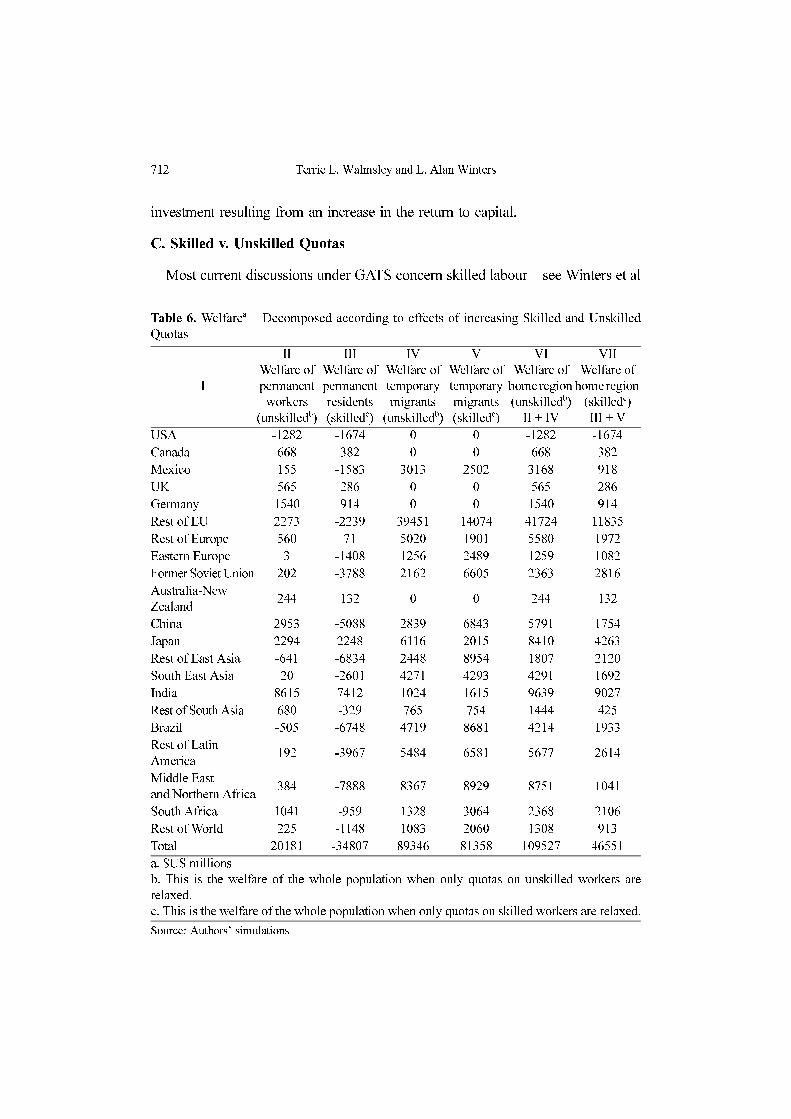
C. Skilled v. Unskilled Quotas
Most current discussions under GATS concern skilled labour – see Winters et al
Table 6. Welfarea – Decomposed according to effects of increasing Skilled and Unskilled
Quotas
I
II
Welfare of
permanent
workers
(unskilledb)
III
Welfare of
permanent
residents
(skilledc)
IV
Welfare of
temporary
migrants
(unskilledb)
V
Welfare of
temporary
migrants
(skilledc)
VI
Welfare of
home region
(unskilledb)
II + IV
VII
Welfare of
home region
(skilledc)
III + V
USA -1282 -1674 0 0 -1282 -1674
Canada 668 382 0 0 668 382
Mexico 155 -1583 3013 2502 3168 918
UK 565 286 0 0 565 286
Germany 1540 914 0 0 1540 914
Rest of EU 2273 -2239 39451 14074 41724 11835
Rest of Europe 560 71 5020 1901 5580 1972
Eastern Europe 3 -1408 1256 2489 1259 1082
Former Soviet Union 202 -3788 2162 6605 2363 2816
Australia-New
Zealand244 132 0 0 244 132
China 2953 -5088 2839 6843 5791 1754
Japan 2294 2248 6116 2015 8410 4263
Rest of East Asia -641 -6834 2448 8954 1807 2120
South East Asia 20 -2601 4271 4293 4291 1692
India 8615 7412 1024 1615 9639 9027
Rest of South Asia 680 -329 765 754 1444 425
Brazil -505 -6748 4719 8681 4214 1933
Rest of Latin
America192 -3967 5484 6581 5677 2614
Middle East
and Northern Africa384 -7888 8367 8929 8751 1041
South Africa 1041 -959 1328 3064 2368 2106
Rest of World 225 -1148 1083 2060 1308 913
Total 20181 -34807 89346 81358 109527 46551
a. $US millions
b. This is the welfare of the whole population when only quotas on unskilled workers are
relaxed.
c. This is the welfare of the whole population when only quotas on skilled workers are relaxed.
Source: Authors’ simulations
Relaxing the Restrictions on the Temporary Movement of Natural Persons 713
(2002). In this section we apply the increases in quotas separately to examine how
much of the gains come from increasing skilled labour quotas and how much from
increasing unskilled labour quotas.
Both the developed and developing countries would benefit more from the
liberalisation of restrictions on unskilled labour than on skilled labour. While the
skilled temporary migrants may earn considerably more overseas than they would
in their home regions, the negative effect of their departure on their home
economies is considerable. Eastern Europe, the Former Soviet Union and East Asia
are cases in which skilled workers obtain greater benefits from working overseas
(Column V of Table 6), than do their unskilled counterparts (Column IV), but in
which the difference is more than offset by the larger losses among permanent
residents from skilled worker mobility (Columns II and III). The reason for this is
that skilled labour is scarce in developing countries, so its loss has more
detrimental effects on production than does the loss of unskilled labour (Column V
of table 7).
For the developed (labour importing) regions relaxing the restrictions on
unskilled labour is also more beneficial in terms of welfare (columns VI and VII in
Table 6) and Real GDP (compare column V in Table 7), than is relaxing them on
skilled workers. The increased supply of unskilled labour reduces unskilled wages
(column III in Table 7), and stimulates most sectors (agricultural and manufactures
and some services), whereas the benefits of increasing skilled labour supplies are
concentrated in a few services sectors. Even though skilled labour is an important
input into the production in most commodities in the developed countries,
unskilled labour is generally more important. The returns to capital and other
inputs (natural resources and land) are increased more as a result of the increase in
unskilled labour quotas, than of those for skilled labour (column IV in Table 7).
Of course, the relative benefits of skilled and unskilled quota relaxations depend
on how far the respective quotas are relaxed. But our results are remarkable in that
we have assumed, based on real data, almost equal increments of skilled and
unskilled labour (8.0 and 8.5 million respectively). It is also interesting that while
developing countries receive a higher share of the benefits of skilled mobility (59
% of $46 billion), they receive absolutely more from unskilled mobility (46 % of
$110 billion).
D. Services Sectors
The GATS concerns only the services sectors. Hence we now assume that all
714 Terrie L. Walmsley and L. Alan Winters
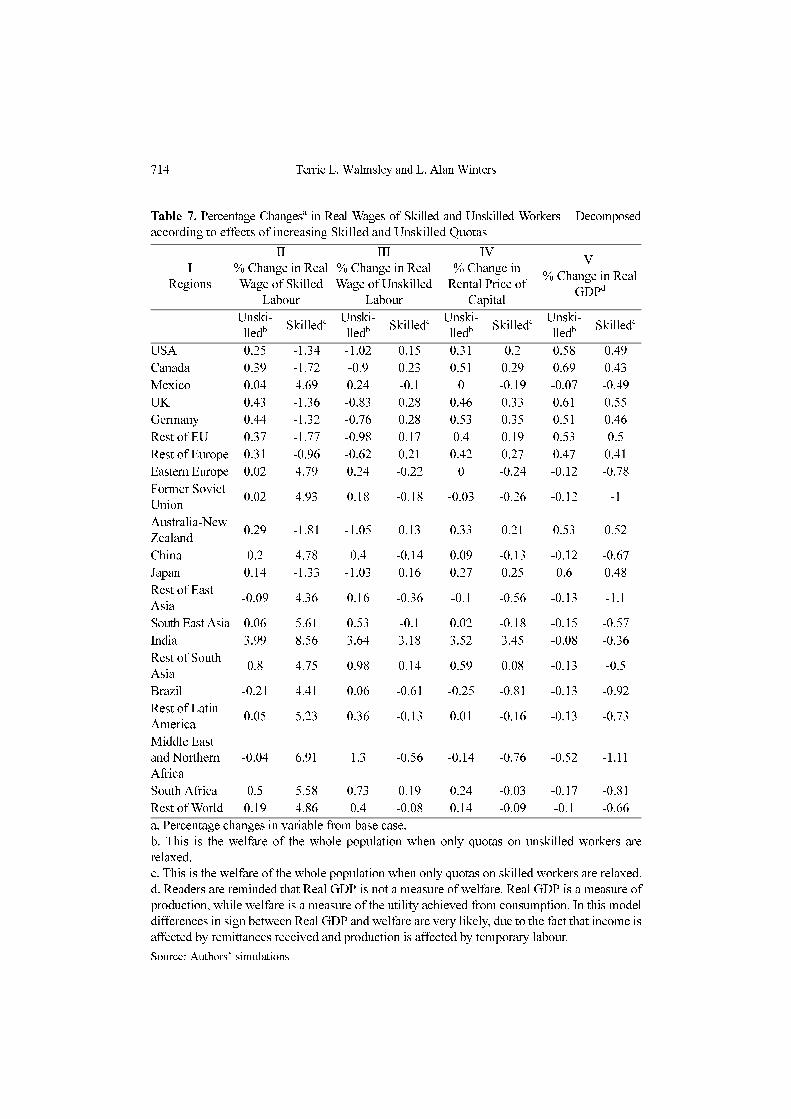
Table 7. Percentage Changesa in Real Wages of Skilled and Unskilled Workers – Decomposed
according to effects of increasing Skilled and Unskilled Quotas
I
Regions
II
% Change in Real
Wage of Skilled
Labour
III
% Change in Real
Wage of Unskilled
Labour
IV
% Change in
Rental Price of
Capital
V
% Change in Real
GDPd
Unski-
lledb Skilledc Unski-
lledb Skilledc Unski-
lledb Skilledc Unski-
lledb Skilledc
USA 0.25 -1.34 -1.02 0.15 0.31 0.2 0.58 0.49
Canada 0.39 -1.72 -0.9 0.23 0.51 0.29 0.69 0.43
Mexico 0.04 4.69 0.24 -0.1 0 -0.19 -0.07 -0.49
UK 0.43 -1.36 -0.83 0.28 0.46 0.33 0.61 0.55
Germany 0.44 -1.32 -0.76 0.28 0.53 0.35 0.51 0.46
Rest of EU 0.37 -1.77 -0.98 0.17 0.4 0.19 0.53 0.5
Rest of Europe 0.31 -0.96 -0.62 0.21 0.42 0.27 0.47 0.41
Eastern Europe 0.02 4.79 0.24 -0.22 0 -0.24 -0.12 -0.78
Former Soviet
Union0.02 4.93 0.18 -0.18 -0.03 -0.26 -0.12 -1
Australia-New
Zealand0.29 -1.81 -1.05 0.13 0.33 0.21 0.53 0.52
China 0.2 4.78 0.4 -0.14 0.09 -0.13 -0.12 -0.67
Japan 0.14 -1.33 -1.03 0.16 0.27 0.25 0.6 0.48
Rest of East
Asia-0.09 4.36 0.16 -0.36 -0.1 -0.56 -0.13 -1.1
South East Asia 0.06 5.61 0.53 -0.1 0.02 -0.18 -0.15 -0.57
India 3.99 8.56 3.64 3.18 3.52 3.45 -0.08 -0.36
Rest of South
Asia0.8 4.75 0.98 0.14 0.59 0.08 -0.13 -0.5
Brazil -0.21 4.41 0.06 -0.61 -0.25 -0.81 -0.13 -0.92
Rest of Latin
America0.05 5.23 0.36 -0.13 0.01 -0.16 -0.13 -0.73
Middle East
and Northern
Africa
-0.04 6.91 1.3 -0.56 -0.14 -0.76 -0.52 -1.11
South Africa 0.5 5.58 0.73 0.19 0.24 -0.03 -0.17 -0.81
Rest of World 0.19 4.86 0.4 -0.08 0.14 -0.09 -0.1 -0.66
a. Percentage changes in variable from base case.
b. This is the welfare of the whole population when only quotas on unskilled workers are
relaxed.
c. This is the welfare of the whole population when only quotas on skilled workers are relaxed.
d. Readers are reminded that Real GDP is not a measure of welfare. Real GDP is a measure of
production, while welfare is a measure of the utility achieved from consumption. In this model
differences in sign between Real GDP and welfare are very likely, due to the fact that income is
affected by remittances received and production is affected by temporary labour.
Source: Authors’ simulations
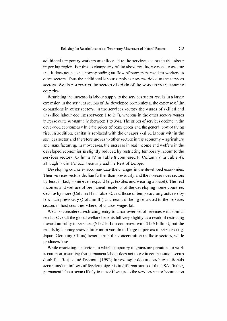
Relaxing the Restrictions on the Temporary Movement of Natural Persons 715
additional temporary workers are allocated to the services sectors in the labour
importing region. For this to change any of the above results, we need to assume
that it does not cause a corresponding outflow of permanent resident workers to
other sectors. Thus the additional labour supply is now restricted to the services
sectors. We do not restrict the sectors of origin of the workers in the sending
countries.
Restricting the increase in labour supply to the services sector results in a larger
expansion in the services sectors of the developed economies at the expense of the
expansions in other sectors. In the services sectors the wages of skilled and
unskilled labour decline (between 1 to 2%), whereas in the other sectors wages
increase quite substantially (between 1 to 3%). The prices of services decline in the
developed economies while the prices of other goods and the general cost of living
rise. In addition, capital is replaced with the cheaper skilled labour within the
services sector and therefore moves to other sectors in the economy – agriculture
and manufacturing. In most cases, the increase in real income and welfare in the
developed economies is slightly reduced by restricting temporary labour to the
services sectors (Column IV in Table 8 compared to Column V in Table 4),
although not in Canada, Germany and the Rest of Europe.
Developing countries accommodate the changes in the developed economies.
Their services sectors decline further than previously and the non-services sectors
by less; in fact, some even expand (e.g. textiles and wearing apparel). The real
incomes and welfare of permanent residents of the developing home countries
decline by more (Column II in Table 8), and those of temporary migrants rise by
less than previously (Column III) as a result of being restricted to the services
sectors in host countries where, of course, wages fall.
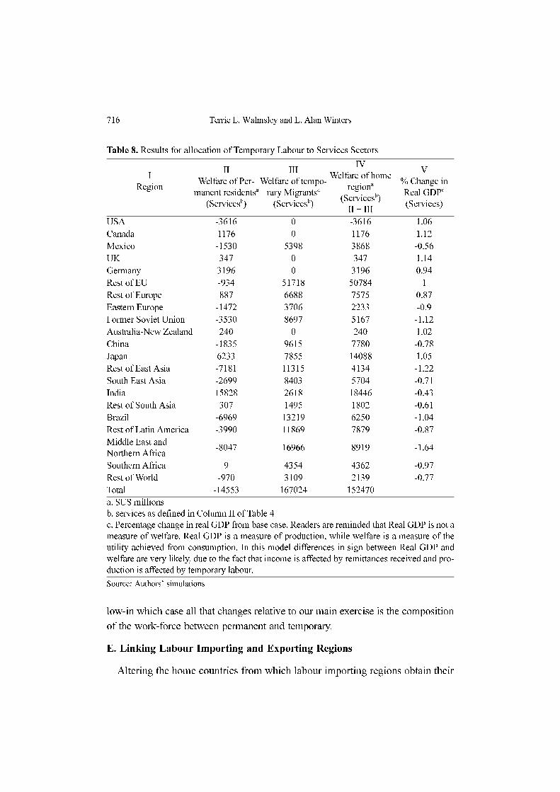
We also considered restricting entry to a narrower set of services with similar
results. Overall the global welfare benefits fall very slightly as a result of restricting
inward mobility to services ($152 billion compared with $156 billion), but the
results by country show a little more variation. Large importers of services (e.g.
Japan, Germany, China) benefit from the concentration on those sectors, while
producers lose.
While restricting the sectors in which temporary migrants are permitted to work
is common, assuming that permanent labour does not move in compensation seems
doubtful. Borjas and Freeman (1992) for example documents how nationals
accommodate inflows of foreign migrants in different states of the USA. Rather,
permanent labour seems likely to move if wages in the services sector became too
716 Terrie L. Walmsley and L. Alan Winters
low-in which case all that changes relative to our main exercise is the composition
of the work-force between permanent and temporary.
E. Linking Labour Importing and Exporting Regions
Altering the home countries from which labour importing regions obtain their
Table 8. Results for allocation of Temporary Labour to Services Sectors
I
Region
II
Welfare of Per-
manent residentsa
(Servicesb)
III
Welfare of tempo-
rary Migrantsa
(Servicesb)
IV
Welfare of home
regiona
(Servicesb)
II + III
V
% Change in
Real GDPd
(Services)
USA -3616 0 -3616 1.06
Canada 1176 0 1176 1.12
Mexico -1530 5398 3868 -0.56
UK 347 0 347 1.14
Germany 3196 0 3196 0.94
Rest of EU -934 51718 50784 1
Rest of Europe 887 6688 7575 0.87
Eastern Europe -1472 3706 2233 -0.9
Former Soviet Union -3530 8697 5167 -1.12
Australia-New Zealand 240 0 240 1.02
China -1835 9615 7780 -0.78
Japan 6233 7855 14088 1.05
Rest of East Asia -7181 11315 4134 -1.22
South East Asia -2699 8403 5704 -0.71
India 15828 2618 18446 -0.43
Rest of South Asia 307 1495 1802 -0.61
Brazil -6969 13219 6250 -1.04
Rest of Latin America -3990 11869 7879 -0.87
Middle East and
Northern Africa-8047 16966 8919 -1.64
Southern Africa 9 4354 4362 -0.97
Rest of World -970 3109 2139 -0.77
Total -14553 167024 152470
a. $US millions
b. services as defined in Column II of Table 4
c. Percentage change in real GDP from base case. Readers are reminded that Real GDP is not a
measure of welfare. Real GDP is a measure of production, while welfare is a measure of the
utility achieved from consumption. In this model differences in sign between Real GDP and
welfare are very likely, due to the fact that income is affected by remittances received and pro-
duction is affected by temporary labour.
Source: Authors’ simulations
Relaxing the Restrictions on the Temporary Movement of Natural Persons 717
temporary labour may also affect the results somewhat, so we now consider
restricting mobility to ‘traditional’ pairs labour importing and exporting regions.
Thus we relax EU and US quotas in turn (by the same amounts as previously), but
restrict the sourcing to their ‘traditional’ labour suppliers – see Table 2.
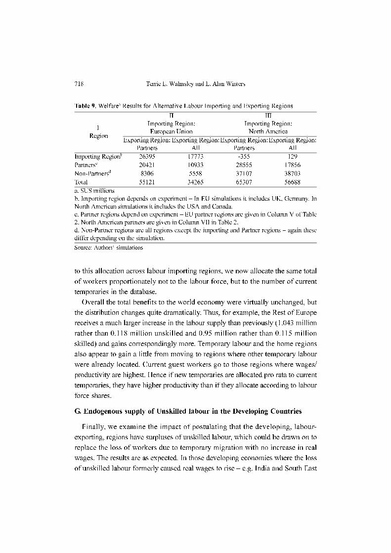
From the perspective of both North America and the EU, taking temporary
migrants only from their traditional partner countries, reduces the welfare benefits
of relaxing quotas.28 The reason is that the partner countries tend to have lower
productivities than the average sending countries so that the increment to
production is less.29
The partner countries, however, generally do better when they are the only
suppliers of temporary labour. Although the gains to the temporary migrants as a
whole are slightly smaller, due to their lower productivities, there are fewer partner
regions to share them. The losses to the permanent residents of the traditional
partner regions are greater as more skilled and unskilled labour move abroad to fill
the quotas. However, overall, taking both the permanent residents and the
temporary migrants into account, the home regions generally gain from the change
(Table 9).
In terms of the non-partners, the welfare loses of the permanent residents are
smaller than previously as they are no longer losing any labour. However, they are
also missing out on the higher incomes and remittances of the temporary labour. In
general, the welfare of the non-partner regions is lower than when they supply
labour – although the extent of the loss depends on the level of development.
F. Quotas increased as a portion of Current Temporary Workers
So far, the shock to the quantity of temporary labour has been equal to 3% of the
labour force of each labour importing region. To test how sensitive the results are
28Note that when comparing the welfare of the EU as the importing region when all regions supply
temporary labour with the case where only the partners supply temporary labour (table 9) it appears as
though welfare increases by more in the partner case. This is because the welfare gain in the partner
case includes a big gain to temporary migrants from the Rest of Europe. If this is removed the results
are consistent with the statement made above.
29In the case of North America, this is mainly because the outflow of workers from the EU is included
in “all” but excluded from “partners”. Likewise, in the case of the EU, North America is included in
“all” but excluded from “partners”. If these developed economies are not included in “all”, productivity
is still lower for “partners” in the EU, since East Asia is not a traditional partners. East Asia has very
high productivity compared to the other labour exporters. In North America, the results would not be
significantly different.
718 Terrie L. Walmsley and L. Alan Winters
to this allocation across labour importing regions, we now allocate the same total
of workers proportionately not to the labour force, but to the number of current
temporaries in the database.
Overall the total benefits to the world economy were virtually unchanged, but
the distribution changes quite dramatically. Thus, for example, the Rest of Europe
receives a much larger increase in the labour supply than previously (1.043 million
rather than 0.118 million unskilled and 0.95 million rather than 0.115 million
skilled) and gains correspondingly more. Temporary labour and the home regions
also appear to gain a little from moving to regions where other temporary labour
were already located. Current guest workers go to those regions where wages/
productivity are highest. Hence if new temporaries are allocated pro rata to current
temporaries, they have higher productivity than if they allocate according to labour
force shares.
G. Endogenous supply of Unskilled labour in the Developing Countries
Finally, we examine the impact of postulating that the developing, labour-
exporting, regions have surpluses of unskilled labour, which could be drawn on to
replace the loss of workers due to temporary migration with no increase in real
wages. The results are as expected. In those developing economies where the loss
of unskilled labour formerly caused real wages to rise – e.g. India and South East
Table 9. Welfarea Results for Alternative Labour Importing and Exporting Regions
I
Region
II
Importing Region:
European Union
III
Importing Region:
North America
Exporting Region:
Partners
Exporting Region:
All
Exporting Region:
Partners
Exporting Region:
All
Importing Regionb 26395 17773 -355 129
Partnersc 20421 10933 28555 17856
Non-Partnersd 8306 5558 37107 38703
Total 55121 34265 65307 56688
a. $US millions
b. Importing region depends on experiment – In EU simulations it includes UK, Germany. In
North American simulations it includes the USA and Canada.
c. Partner regions depend on experiment – EU partner regions are given in Column V of Table
2. North American partners are given in Column VII in Table 2.
d. Non-Partner regions are all regions except the importing and Partner regions – again these
differ depending on the simulation.
Source: Authors’ simulations
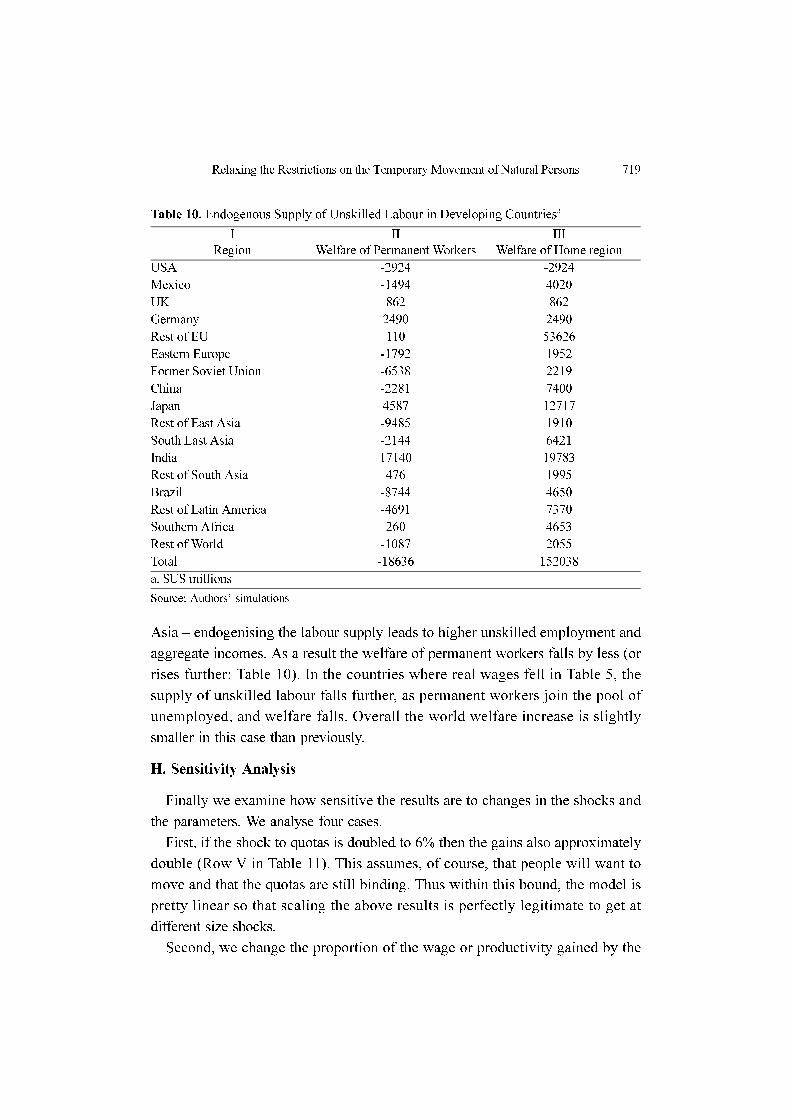
Relaxing the Restrictions on the Temporary Movement of Natural Persons 719
Asia – endogenising the labour supply leads to higher unskilled employment and
aggregate incomes. As a result the welfare of permanent workers falls by less (or
rises further: Table 10). In the countries where real wages fell in Table 5, the
supply of unskilled labour falls further, as permanent workers join the pool of
unemployed, and welfare falls. Overall the world welfare increase is slightly
smaller in this case than previously.
H. Sensitivity Analysis
Finally we examine how sensitive the results are to changes in the shocks and
the parameters. We analyse four cases.
First, if the shock to quotas is doubled to 6% then the gains also approximately
double (Row V in Table 11). This assumes, of course, that people will want to
move and that the quotas are still binding. Thus within this bound, the model is
pretty linear so that scaling the above results is perfectly legitimate to get at
different size shocks.
Second, we change the proportion of the wage or productivity gained by the
Table 10. Endogenous Supply of Unskilled Labour in Developing Countriesa
I
Region
II
Welfare of Permanent Workers
III
Welfare of Home region
USA -2924 -2924
Mexico -1494 4020
UK 862 862
Germany 2490 2490
Rest of EU 110 53626
Eastern Europe -1792 1952
Former Soviet Union -6538 2219
China -2281 7400
Japan 4587 12717
Rest of East Asia -9485 1910
South East Asia -2144 6421
India 17140 19783
Rest of South Asia 476 1995
Brazil -8744 4650
Rest of Latin America -4691 7370
Southern Africa 260 4653
Rest of World -1087 2055
Total -18636 152038
a. $US millions
Source: Authors’ simulations
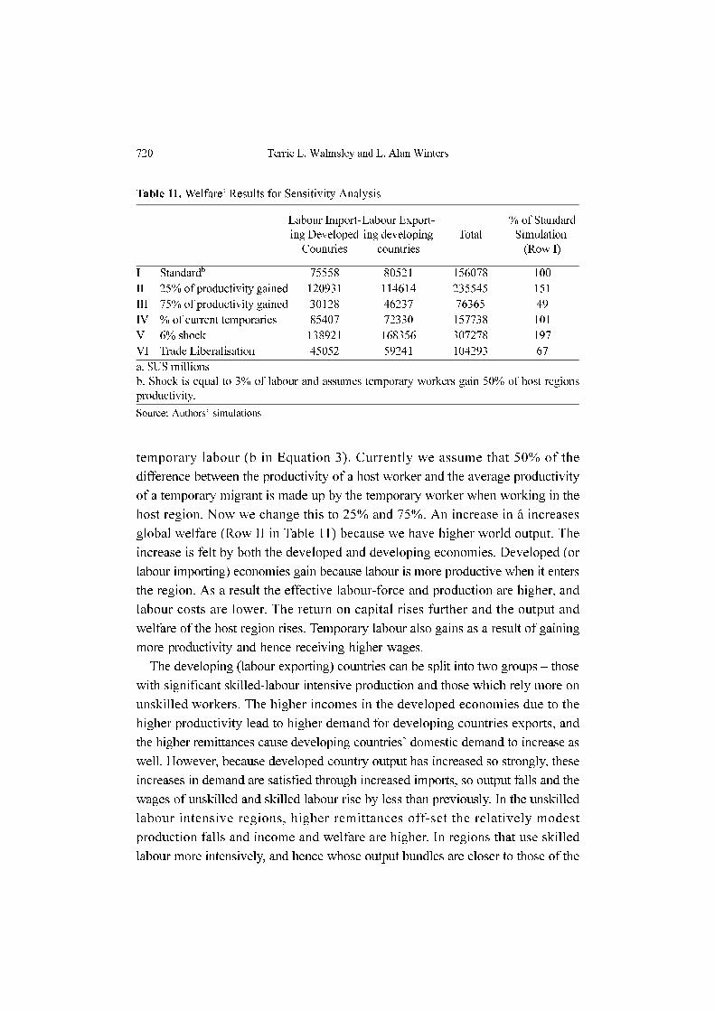
720 Terrie L. Walmsley and L. Alan Winters
temporary labour (b in Equation 3). Currently we assume that 50% of the
difference between the productivity of a host worker and the average productivity
of a temporary migrant is made up by the temporary worker when working in the
host region. Now we change this to 25% and 75%. An increase in â increases
global welfare (Row II in Table 11) because we have higher world output. The
increase is felt by both the developed and developing economies. Developed (or
labour importing) economies gain because labour is more productive when it enters
the region. As a result the effective labour-force and production are higher, and
labour costs are lower. The return on capital rises further and the output and
welfare of the host region rises. Temporary labour also gains as a result of gaining
more productivity and hence receiving higher wages.
The developing (labour exporting) countries can be split into two groups – those
with significant skilled-labour intensive production and those which rely more on
unskilled workers. The higher incomes in the developed economies due to the
higher productivity lead to higher demand for developing countries exports, and
the higher remittances cause developing countries’ domestic demand to increase as
well. However, because developed country output has increased so strongly, these
increases in demand are satisfied through increased imports, so output falls and the
wages of unskilled and skilled labour rise by less than previously. In the unskilled
labour intensive regions, higher remittances off-set the relatively modest
production falls and income and welfare are higher. In regions that use skilled
labour more intensively, and hence whose output bundles are closer to those of the
Table 11. Welfarea Results for Sensitivity Analysis
Labour Import-
ing Developed
Countries
Labour Export-
ing developing
countries
Total
% of Standard
Simulation
(Row I)
I Standardb 75558 80521 156078 100
II 25% of productivity gained 120931 114614 235545 151
III 75% of productivity gained 30128 46237 76365 49
IV % of current temporaries 85407 72330 157738 101
V 6% shock 138921 168356 307278 197
VI Trade Liberalisation 45052 59241 104293 67
a. $US millions
b. Shock is equal to 3% of labour and assumes temporary workers gain 50% of host regions
productivity.
Source: Authors’ simulations
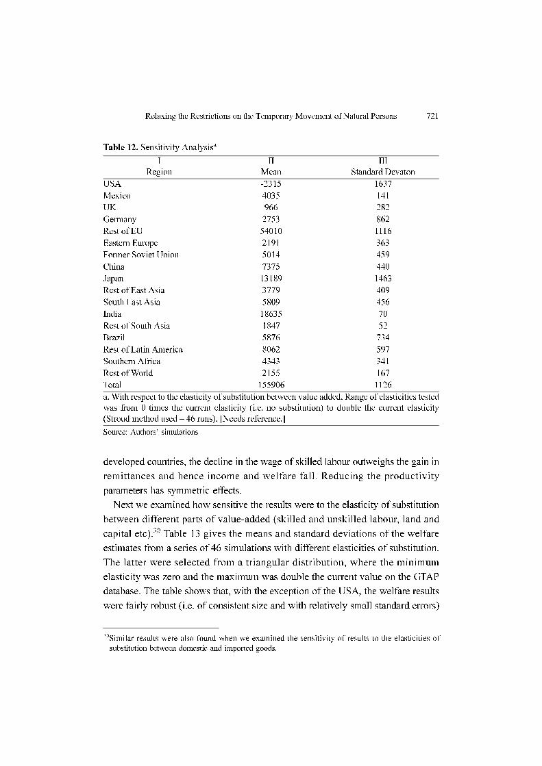
Relaxing the Restrictions on the Temporary Movement of Natural Persons 721
developed countries, the decline in the wage of skilled labour outweighs the gain in
remittances and hence income and welfare fall. Reducing the productivity
parameters has symmetric effects.
Next we examined how sensitive the results were to the elasticity of substitution
between different parts of value-added (skilled and unskilled labour, land and
capital etc).30 Table 13 gives the means and standard deviations of the welfare
estimates from a series of 46 simulations with different elasticities of substitution.
The latter were selected from a triangular distribution, where the minimum
elasticity was zero and the maximum was double the current value on the GTAP
database. The table shows that, with the exception of the USA, the welfare results
were fairly robust (i.e. of consistent size and with relatively small standard errors)
Table 12. Sensitivity Analysisa
I
Region
II
Mean
III
Standard Devaton
USA -2315 1637
Mexico 4035 141
UK 966 282
Germany 2753 862
Rest of EU 54010 1116
Eastern Europe 2191 363
Former Soviet Union 5014 459
China 7375 440
Japan 13189 1463
Rest of East Asia 3779 409
South East Asia 5809 456
India 18635 70
Rest of South Asia 1847 52
Brazil 5876 734
Rest of Latin America 8062 597
Southern Africa 4343 341
Rest of World 2155 167
Total 155906 1126
a. With respect to the elasticity of substitution between value added. Range of elasticities tested
was from 0 times the current elasticity (i.e. no substitution) to double the current elasticity
(Stroud method used – 46 runs). [Needs reference.]
Source: Authors’ simulations
30Similar results were also found when we examined the sensitivity of results to the elasticities of
substitution between domestic and imported goods.
722 Terrie L. Walmsley and L. Alan Winters
to changes in the elasticity of substitution. In the case of the USA, we cannot be
confident of the sign of the effect but as noted above this is almost certainly
because of the idiosyncracies of the US data.
Welfare varies with the elasticity of substitution within value-added because the
latter affects the magnitude (but not necessarily the direction) of the return on
value-added. For example, with greater substitution smaller increases in the rental
price of capital are required to absorb the given increases in labour. This, in turn,
leads to smaller increases in income and welfare. Likewise, when the elasticities
are reduced, the rental price of capital rises more strongly. The effect of these
changes in the elasticity of substitution between elements of value-added are
greatest in the developed economies, where factor shares are more balanced and
hence substitutability between them is of greater importance than in developing
economies, where the main factor of production is unskilled labour.
Finally, the average portions of wages sent home as remittances are determined
by the remittance data collected and are assumed to be constant. In the initial data
an average of 20% of wages was sent home. Here we investigate how different the
results would be if 40% of wages were sent home.31 World welfare does not alter
as a result of the increase in remittances, but there are two important implications
for their distribution. First, the transfer of income to permanent residents of the
labour exporting regions raises their welfare, although at the expense of that of the
temporary migrants. Overall the welfare of the developing economies stays the
same or rises. Second, the welfare of the developed economies falls, as less income
is spent in these countries.
IV. Conclusion
Restrictions on the movement of natural persons are increasingly being
recognised as a severe impediment to trade in services. The relaxation of these
restrictions could result in important benefits to the world as a whole and in
particular to the suppliers of this labour. In this paper a model was developed to
analyse the effect of relaxing these restrictions on the movement of labour.
The model takes into account a number of important issues related to the
movement of labour, including:
31This was achieved by assuming that our initial data on remittances were inaccurate and did not take
account of all remittances sent home. Remittances were therefore doubled and the base data
recalibrated.
Relaxing the Restrictions on the Temporary Movement of Natural Persons 723
a) differences in the productivities of temporary and permanent labour;
b) the importance of remittances on home country income;
c) the calculation of income and welfare of permanent and temporary labour;
and
d) the movement of labour into particular sectors in the host region.
We have treated the temporary movement of natural persons as a shift in labour
services to the host regions rather than as a question of exporting services as is
implied by the institutional framework in which such liberalisations are likely to
take place. Although temporary mobility is not a migration issue, temporary
workers are assumed to produce, earn wages, pay taxes and consume in the host
country, as well as send remittances back to their home countries. Moreover, we
assume that the jobs so created are permanent even though the incumbents are not.
In our main exercise, quotas on the number of temporary workers permitted into
the developed economies are increased by 3% of the developed economies’ labour
forces. The increase in world welfare is substantial and far exceeds the benefits
expected from any remaining trade liberalisation. Overall, the developing countries
gain most from the increase in quotas, highlighting again that this is an important
issue for development. The developed economies also experience gains in welfare,
however, so the liberalisation would be no mere act of charity: their real wages fall,
but increases in the returns to capital and other factors more than offset this,
leaving net gains overall. It is also interesting to note that while most of the
progress in policy discussions have concerned increasing the mobility of skilled
labour, it is the relaxation of quotas on unskilled labour that generates the most
benefits. This is the case for both the developed and developing economies.
Acknowledgements
This paper was supported by the Commonwealth Secretariat, to whom we most
grateful. Its views and opinions are the authors’ and should in no way be attributed
to the Commonwealth Secretariat or its member countries. We are grateful to
Roman Grynberg, Zhen Kun Wang and colleagues at the University of Sussex for
comments on earlier drafts of this work.
Received 7 September 2004, Accepted 29 December 2004
724 Terrie L. Walmsley and L. Alan Winters
References
Borjas, G. J. (1995), “The economic benefits from immigration”, Journal of Economic
Perspectives, vol 9(2), pp. 3-22.
Borjas, G. J. (2000): Labour Economics, 2nd Edition, McGraw-Hill, Boston.
Borjas, G. J. and Freeman (eds) (1992): Immigration and the Workforce: Economic
Consequences for the US and Source Areas, University of Chicago Press: Chicago.
Davis D and Weinstein D (2002), “Technological Superiority and the Losses from
Migration”, NBER Working paper No. 8971.
Dimaranan, B. V. and R. A. McDougall, (2001): Global Trade Analysis and Production:
The GTAP 5 Data Base, Center for Global Trade Analysis, Purdue, University, West
Lafayette, IN, USA. Available at: http://www.agecon.purdue.edu/GTAP/databases/
v5/ v5_doco.asp
Faini R., De Melo, J., and K. F. Zimmerman, (1999): Globalisation and Migratory
pressures from the developing countries: A Simulation Analysis. In Migration: The
Controversies and the Evidence, Faini R., De Melo, J., and K. F. Zimmerman (eds),
Cambridge University Press: Cambridge.
Grynberg, R. (2001): Liberalising Global Labour Markets: Recent Developments at the
WTO, mimeo.
Hamilton, B., and Whalley J. (1984): “Efficiency and Distributional Implications of
Global Restrictions on Labour Mobility: Calculations and Policy Implications”
Journal of Development Economics 14 (1-2), 61-75, Elsevier Science Publishers
(North Holland).
Hertel, T. W. (ed), (1997): Global Trade Analysis: Modeling and Applications Cambridge:
Cambridge University Press.
International Labour Organisation (ILO): International Labour Migration Database 1986
onwards. Available at: http://www.ilo.org/public/english/protection/migrant/
ilmdb.htm.
Walmsley, T. L. (2001): Modelling the Movement of Natural Persons, Mimeo.
Walmsley, T. L. (2002): “Incorporating International Capital Ownership into a Global
CGE Model”, Economic Modelling, Nov. 19(5).
Walmsley, T. L. (1999): Steady-State Comparative Statics with the GTAP Model: The
Long-Run Effects of Asia-Pacific Trade Liberalisation, Thesis submitted for Doctoral
studies at Monash University, Clayton, Vic, 3168, Australia.
Winters, L. A., T. L. Walmsley, Z. K. Wang and Grynberg, R. (2002): Liberalising the
Temporary Movement of Natural Persons, Economics Discussion Paper No ,
University of Sussex.
Relaxing the Restrictions on the Temporary Movement of Natural Persons 725
Appendix 1
In this appendix we show an alternative distribution of welfare gains across
temporary migrants. In this alternative scenario it is assumed that the initial
temporary migrants in the data base are not allowed to move to take up quota
places in the labour exporting region.
Under this assumption the total change in income of all temporary workers
(initial32 or new33) is determined as in the main exercise. Following this the income
of the initial temporary migrants is found by assuming that their wage falls with the
general fall in wages in their host regions. The income of the initial temporary
migrants is then subtracted from the total income of all temporary migrants to
determine the income of the new temporary migrants. This income is then divided
across the home regions of the new temporary migrants according to their shares in
that flow. The relevant income and the average price in the host regions is then used
to determined the change in welfare of the initial and new temporary migrants.
Table A1.1 shows that the welfare of temporary workers (II), permanent
residents (IV) and of the host region (VI) has not changed as a result of this
alternative distribution,34 and that neither has the total welfare of temporary
migrants. However, the distribution of this latter welfare has altered significantly
(compare column III in Table 4 with column III in Table A1.1). In the ‘Rest of EU’
and the other labour importing regions the welfare of the temporary migrants has
fallen by $US13billion as a result of a lower average wage in their host regions as
compared to previous when welfare rose by $US53billion. Thus under this
assumption the ‘Rest of EU’ as a home region loses. This result offers an
additional reason to question the assumption made here. The losses made by these
mobile temporary migrants will be significant enough at least to prompt them to
consider moving to take up the new quota places hence undermining the
assumption made here and validating that in the main text.
32Initial temporary migrants are defined as those migrants in the labour exporting economies who lived
abroad prior to the new shocks. I.e. the temporary migrants in the initial data base. Unfortunately the
method used is crude and it was not possible to include those current temporaries in the labour
exporting regions.
33New temporary migrants are those workers from the labour exporting regions who move as a result of
the increase in quotas in the labour importing regions.
34In fact nothing has changed other than the welfare of the temporary migrants by home region. This is
simply a different distribution method.
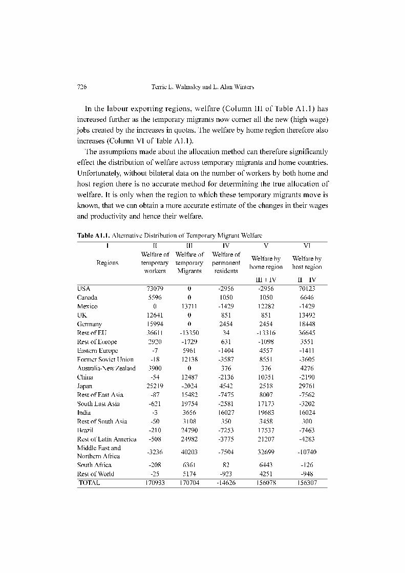
726 Terrie L. Walmsley and L. Alan Winters
In the labour exporting regions, welfare (Column III of Table A1.1) has
increased further as the temporary migrants now corner all the new (high wage)
jobs created by the increases in quotas. The welfare by home region therefore also
increases (Column VI of Table A1.1).
The assumptions made about the allocation method can therefore significantly
effect the distribution of welfare across temporary migrants and home countries.
Unfortunately, without bilateral data on the number of workers by both home and
host region there is no accurate method for determining the true allocation of
welfare. It is only when the region to which these temporary migrants move is
known, that we can obtain a more accurate estimate of the changes in their wages
and productivity and hence their welfare.
Table A1.1. Alternative Distribution of Temporary Migrant Welfare
I II III IV V VI
Regions
Welfare of
temporary
workers
Welfare of
temporary
Migrants
Welfare of
permanent
residents
Welfare by
home region
Welfare by
host region
III + IV II + IV
USA 73079 0 -2956 -2956 70123
Canada 5596 0 1050 1050 6646
Mexico 0 13711 -1429 12282 -1429
UK 12641 0 851 851 13492
Germany 15994 0 2454 2454 18448
Rest of EU 36611 -13350 34 -13316 36645
Rest of Europe 2920 -1729 631 -1098 3551
Eastern Europe -7 5961 -1404 4557 -1411
Former Soviet Union -18 12138 -3587 8551 -3605
Australia-New Zealand 3900 0 376 376 4276
China -54 12487 -2136 10351 -2190
Japan 25219 -2024 4542 2518 29761
Rest of East Asia -87 15482 -7475 8007 -7562
South East Asia -621 19754 -2581 17173 -3202
India -3 3656 16027 19683 16024
Rest of South Asia -50 3108 350 3458 300
Brazil -210 24790 -7253 17537 -7463
Rest of Latin America -508 24982 -3775 21207 -4283
Middle East and
Northern Africa-3236 40203 -7504 32699 -10740
South Africa -208 6361 82 6443 -126
Rest of World -25 5174 -923 4251 -948
TOTAL 170933 170704 -14626 156078 156307