Release 1.0 Florian Wellmann, Sam Thiele · 3.2 Loading Noddy output ﬁles. . . . . . . . . . . . . . . . . . . . . . . . . . . . . . . . . . . . .12

pynoddy DocumentationRelease 1.0

Florian Wellmann, Sam Thiele

Aug 26, 2017

Contents

1 pynoddy 31.1 What is pynoddy . . . . . . . . . . . . . . . . . . . . . . . . . . . . . . . . . . . . . . . . . . 31.2 What is Noddy? . . . . . . . . . . . . . . . . . . . . . . . . . . . . . . . . . . . . . . . . . . . 31.3 Installation . . . . . . . . . . . . . . . . . . . . . . . . . . . . . . . . . . . . . . . . . . . . . . 31.4 Installation of the pynoddy package . . . . . . . . . . . . . . . . . . . . . . . . . . . . . . . . 31.5 Installation of Noddy . . . . . . . . . . . . . . . . . . . . . . . . . . . . . . . . . . . . . . . . 41.6 Using a pre-compiled version of Noddy . . . . . . . . . . . . . . . . . . . . . . . . . . . . . . 41.7 Compiling Noddy from source files (recommended installation) . . . . . . . . . . . . . . . . . . 41.8 Placing the executable noddy in the Path . . . . . . . . . . . . . . . . . . . . . . . . . . . . . . 51.9 Noddy executable and GUI for Windows . . . . . . . . . . . . . . . . . . . . . . . . . . . . . . 51.10 Testing the installation . . . . . . . . . . . . . . . . . . . . . . . . . . . . . . . . . . . . . . . . 51.11 Testing noddy . . . . . . . . . . . . . . . . . . . . . . . . . . . . . . . . . . . . . . . . . . . . 51.12 Testing pynoddy . . . . . . . . . . . . . . . . . . . . . . . . . . . . . . . . . . . . . . . . . . 61.13 How to get started . . . . . . . . . . . . . . . . . . . . . . . . . . . . . . . . . . . . . . . . . . 61.14 Tutorial Jupyter notebooks . . . . . . . . . . . . . . . . . . . . . . . . . . . . . . . . . . . . . . 61.15 The Atlas of Strutural Geophysics . . . . . . . . . . . . . . . . . . . . . . . . . . . . . . . . . . 61.16 Documentation . . . . . . . . . . . . . . . . . . . . . . . . . . . . . . . . . . . . . . . . . . . . 61.17 Technical Notes . . . . . . . . . . . . . . . . . . . . . . . . . . . . . . . . . . . . . . . . . . . 71.18 Dependencies . . . . . . . . . . . . . . . . . . . . . . . . . . . . . . . . . . . . . . . . . . . . . 71.19 3-D Visualisation . . . . . . . . . . . . . . . . . . . . . . . . . . . . . . . . . . . . . . . . . . . 71.20 References . . . . . . . . . . . . . . . . . . . . . . . . . . . . . . . . . . . . . . . . . . . . . . 7

2 pynoddy.noddy module 9

3 Simulation of a Noddy history and visualisation of output 113.1 Compute the model . . . . . . . . . . . . . . . . . . . . . . . . . . . . . . . . . . . . . . . . . . 113.2 Loading Noddy output files . . . . . . . . . . . . . . . . . . . . . . . . . . . . . . . . . . . . . 123.3 Plotting sections through the model . . . . . . . . . . . . . . . . . . . . . . . . . . . . . . . . . 123.4 Export model to VTK . . . . . . . . . . . . . . . . . . . . . . . . . . . . . . . . . . . . . . . . 13

4 Change Noddy input file and recompute model 154.1 Get basic information on the model . . . . . . . . . . . . . . . . . . . . . . . . . . . . . . . . . 164.2 Change model cube size and recompute model . . . . . . . . . . . . . . . . . . . . . . . . . . . 174.3 Estimating computation time for a high-resolution model . . . . . . . . . . . . . . . . . . . . . . 184.4 Simple convergence study . . . . . . . . . . . . . . . . . . . . . . . . . . . . . . . . . . . . . . 21

5 Geological events in pynoddy: organisation and adpatiation 235.1 Loading events from a Noddy history . . . . . . . . . . . . . . . . . . . . . . . . . . . . . . . . 235.2 Changing aspects of geological events . . . . . . . . . . . . . . . . . . . . . . . . . . . . . . . . 255.3 Changing the order of geological events . . . . . . . . . . . . . . . . . . . . . . . . . . . . . . . 255.4 Determining the stratigraphic difference between two models . . . . . . . . . . . . . . . . . . . 27

i

6 Creating a model from scratch 296.1 Defining a stratigraphy . . . . . . . . . . . . . . . . . . . . . . . . . . . . . . . . . . . . . . . . 296.2 Add a fault event . . . . . . . . . . . . . . . . . . . . . . . . . . . . . . . . . . . . . . . . . . . 306.3 Complete Model Set-up . . . . . . . . . . . . . . . . . . . . . . . . . . . . . . . . . . . . . . . 32

7 Read and Visualise Geophysical Potential-Fields 357.1 Read history file from Virtual Explorer . . . . . . . . . . . . . . . . . . . . . . . . . . . . . . . 357.2 Visualise calculated geophysical fields . . . . . . . . . . . . . . . . . . . . . . . . . . . . . . . 377.3 Change history and compare gravity . . . . . . . . . . . . . . . . . . . . . . . . . . . . . . . . . 387.4 Figure with all results . . . . . . . . . . . . . . . . . . . . . . . . . . . . . . . . . . . . . . . . 42

8 Reproducible Experiments with pynoddy 458.1 Defining an experiment . . . . . . . . . . . . . . . . . . . . . . . . . . . . . . . . . . . . . . . 458.2 Loading an example model from the Atlas of Structural Geophysics . . . . . . . . . . . . . . . . 46

9 Gippsland Basin Uncertainty Study 519.1 The Gippsland Basin Model . . . . . . . . . . . . . . . . . . . . . . . . . . . . . . . . . . . . . 519.2 Generate randomised model realisations . . . . . . . . . . . . . . . . . . . . . . . . . . . . . . . 529.3 Exporting results to VTK for visualisation . . . . . . . . . . . . . . . . . . . . . . . . . . . . . 53

10 Sensitivity Analysis 5510.1 Theory: local sensitivity analysis . . . . . . . . . . . . . . . . . . . . . . . . . . . . . . . . . . 5510.2 Defining the responses . . . . . . . . . . . . . . . . . . . . . . . . . . . . . . . . . . . . . . . . 5510.3 Setting up the base model . . . . . . . . . . . . . . . . . . . . . . . . . . . . . . . . . . . . . . 5610.4 Define parameter uncertainties . . . . . . . . . . . . . . . . . . . . . . . . . . . . . . . . . . . . 5710.5 Calculate total stratigraphic distance . . . . . . . . . . . . . . . . . . . . . . . . . . . . . . . . . 5810.6 Function to modify parameters . . . . . . . . . . . . . . . . . . . . . . . . . . . . . . . . . . . . 5810.7 Full sensitivity analysis . . . . . . . . . . . . . . . . . . . . . . . . . . . . . . . . . . . . . . . 59

11 Simulation of a Noddy history and analysis of its voxel topology 6311.1 Compute the model . . . . . . . . . . . . . . . . . . . . . . . . . . . . . . . . . . . . . . . . . . 6311.2 Loading Topology output files . . . . . . . . . . . . . . . . . . . . . . . . . . . . . . . . . . . . 64

12 Fault shapes 67

13 Pynoddy modules, classes and functions 6913.1 Basic modules (low-level access) . . . . . . . . . . . . . . . . . . . . . . . . . . . . . . . . . . 6913.2 Modules for Kinematic experiments . . . . . . . . . . . . . . . . . . . . . . . . . . . . . . . . . 69

ii

pynoddy Documentation, Release 1.0

Contents:

Contents

• pynoddy

– What is pynoddy

– What is Noddy?

– Installation

– Installation of the pynoddy package

– Installation of Noddy

– Using a pre-compiled version of Noddy

– Compiling Noddy from source files (recommended installation)

– Placing the executable noddy in the Path

– Noddy executable and GUI for Windows

– Testing the installation

– Testing noddy

– Testing pynoddy

– How to get started

– Tutorial Jupyter notebooks

– The Atlas of Strutural Geophysics

– Documentation

– Technical Notes

– Dependencies

– 3-D Visualisation

– References

Contents 1


2 Contents

CHAPTER 1

pynoddy

What is pynoddy

pynoddy is a python package to write, change, and analyse kinematic geological modelling simulations. Itprovides methods to define, load, modify, and safe kinematic models for simulation with Noddy. In addition, thepackage contains an extensive range for postprocessing of results. One main aspect of pynoddy is that it enablesthe encapsulation of full scientific kinematic modelling experiments for full reproducibility of results.

What is Noddy?

Noddy itself is a kinematic modelling program written by Mark Jessell [1][2] to simulate the effect of subsequentgeological events (folding, unconformities, faulting, etc.) on a primary sedimentary pile. A typical example wouldbe:

1. Create a sedimentary pile with defined thicknesses for multiple formations

2. Add a folding event (for example simple sinoidal folding, but complex methods are possible!)

3. Add an unconformity and, above it, a new stratigraphy

4. Finally, add a sequence of late faults affecting the entire system.

The result could look something like this:

Noddy has been used to generate models for teaching and interpretation purposes, but also for scientific studies(e.g. [3]).

Installation

Installation of the pynoddy package

A successful installation of pynoddy requires two steps:

1. An installation of the python modules in the package pynoddy

2. The existance of an executable Noddy(.exe) program

3


Installation of the first part is straight-forward:

For the best (and most complete) installation, we suggest to clone the pynoddy repository on:

https://github.com/flohorovicic/pynoddy

To install pynoddy simply run:

python setup.py install

sufficient privileges are required (i.e. run in sudo with MacOSX/ Linux and set permissions on Windows)

The pynoddy packages themselves can also be installed directly from the Python Package Index (pypi.org) viapip:

pip install pynoddy

A Windows installer is also available on the Pypi page:

https://pypi.python.org/pypi/pynoddy/

Installation of Noddy

Noddy is a command line program, written in C, that performs the kinematic simulation itself. The programcompilation is platform dependent, and therefore several ways for installation are possible (see below informationfor specific platforms).

Using a pre-compiled version of Noddy

The easy way to obtain a executable version of Noddy is simply to download the appropriate version for youroperating system. Currently, these executables versions are also stored on github (check the up-to-date onlinedocumentation if this should not anymore be the case) in the directory:

https://github.com/flohorovicic/pynoddy/tree/master/noddyapp

Furthermore, the executables for Windows are also available for download on the webpage:

http://www.tectonique.net/pynoddy

Download the appropriate app, rename it to noddy or noddy.exe and place it into a folder that is in your localenvironment path variable. If you are not sure if a folder is in the PATH or would like to add new one, see belowfor more information.

Compiling Noddy from source files (recommended installation)

The source code for the executable Noddy is located in the repository directory noddy. In order to performthe installation, a gcc compiler is required. This compiler should be available on Linux and MacOSX operatingsystems. On Windows, one possibility is to install MinGW. Otherwise, the code requires no specific libraries.

Note for MacOSX users: some header files have to be adapted to avoid conflicts with local libraries. The requiredadaptations are executed when running the script:

> adjust_for_MacOSX.sh

The compilation is then performed (in a Linux, MacOSX, or Windows MinGW terminal) with the command:

> compile.sh

Compilation usually produces multiple warnings, but should otherwise proceed successfully.

4 Chapter 1. pynoddy

https://github.com/flohorovicic/pynoddy

https://pypi.python.org/pypi/pynoddy/

https://github.com/flohorovicic/pynoddy/tree/master/noddyapp

http://www.tectonique.net/pynoddy


Placing the executable noddy in the Path

For the most general installation, the executable of Noddy should be placed in a folder that can be located fromany terminal application in the system. This (usually) means that the folder with the executable has to be in thePATH environment variable. On Linux and MacOSX, a path can simply be added by:

> export PATH-"path/to/executable/:\$PATH"

Note that this command should be placed into your .bash_profile file to ensure that the path is added wheneveryou start a new Python script.

On windows, adding a folder to the local environment variable Path is usually done through the System ControlPanel (Start - Settings - Control Panel - System). in Advanced mode, open the Environment Variables sub-menu,and find the variable Path. Click to edit the variable, and add the location of your folder to this path.

Noddy executable and GUI for Windows

The original graphical user interface for Noddy and the compiled executable program for Windows can be ob-tained from:

http://tinyurl.com/noddy-site

This site also contains the source code, as well as extensive documentation and tutorial material concerning theoriginal implementation of the software, as well as more technical details on the modelling method itself.

Testing the installation

Testing noddy

Simply test the installation by running the generated (or downloaded) executable in a terminal window (on Win-dows: cmd):

> noddy

or (depending on your compilation or naming convention):

> noddy.exe

Which should produce the general output:

Arguments <historyfile> <outputfile> <calc_mode>:BLOCKGEOPHYSICSSURFACESBLOCK_GEOPHYSBLOCK_SURFACESTOPOLOGYANOM_FROM_BLOCKALL

Note: if the executable is correctly placed in a folder which is recognised by the (Environment) path variable, thenyou should be able to run Noddy from any directory. If this is not the case, please check if it is correctly placedin the path (see above).

1.8. Placing the executable noddy in the Path 5

http://tinyurl.com/noddy-site


Testing pynoddy

The pynoddy package contains a set of tests which can be executed in the standard Python testing environment.If you cloned or downloaded the repository, then these tests can directly be performed through the setup script:

> python setup.py test

Of specific relevance is the test that determines if the noddy(.exe) executable is correctly accessible frompynoddy. If this is the case, then the compute_model test should return:

test_compute_model (test.TestHistory) ... ok}

If this test is not ok, then please check carefully the installation of the noddy(.exe) executable.

If all tests are successful, you are ready to go!

How to get started

Tutorial Jupyter notebooks

The best way to get started with pynoddy is to have a look at the IPython notebooks in pynoddy/docs/notebooks.The numbered notebooks are those that are part of the documentation, and a good point to get started.

The notebooks require an installed Jupyter notebook. More information here:

https://jupyter.org

The notebook can be installed via pip or conda.

The Atlas of Strutural Geophysics

The Atlas of Structural Geophysics contains a collection of structural models, together with their expression asgeophysical potential fields (gravity and magnetics), with a focus on guiding the interpretation of observed featuresin potential-field maps.

The atlas is currently available on:

http://tectonique.net/asg

The structural models are created with Noddy and the history files can be downloaded from the atlas. Models fromthis Atlas can directly be loaded with pynoddy. See example notebooks and documentation for more details.

Documentation

An updated version of the documentation is available within the pynoddy repository (pynoddy/docs).

In addition, an online html version of the documentation is also hosted on readthedocs:

http://pynoddy.readthedocs.org


https://jupyter.org

http://tectonique.net/asg

http://pynoddy.readthedocs.org


Technical Notes

Dependencies

pynoddy depends on several standard Python packages that should be shipped with any standard distribution(and are easy to install, otherwise):

• numpy

• matplotlib

• pickle

The uncertainty analysis, quantification, and visualisation methods based on information theory are implementedin the python package pygeoinfo. This package is available on github and part of the python package index. It isautomatically installed with the setup script provided with this package.

In addition, to export model results for full 3-D visualisation with VTK, the pyevtk package is used, available onbitbucket:

https://bitbucket.org/pauloh/pyevtk/src/9c19e3a54d1e?at-v0.1.0

The package is automatically downloaded and installed when running python setup.py install.

3-D Visualisation

At this stage, we do not supply methods for 3-D visualisation in python (although this may change in the future).However, we provide methods to export results into a VTK format. Exported files can then be viewed with thehighly functional VTK viewers, and several free options are available, for example:

• Paraview: http://www.paraview.org

• Visit: https://wci.llnl.gov/simulation/computer-codes/visit/

• Mayavi: http://docs.enthought.com/mayavi/mayavi/

License ~~~~~~-

pynoddy is free software (see license file included in the repository). Please attribute the work when you use itand cite the publication if you use it in a scientific context - feel free to change and adapt it otherwise!

References

[1] Mark W. Jessell. Noddy, an interactive map creation package. Unpublished MSc Thesis, University of London.1981.

[2] Mark W. Jessell, Rick K. Valenta, Structural geophysics: Integrated structural and geophysical modelling,In: Declan G. De Paor, Editor(s), Computer Methods in the Geosciences, Pergamon, 1996, Volume 15, Pages303-324, ISSN 1874-561X, ISBN 9780080424309, http://dx.doi.org/10.1016/S1874-561X(96)80027-7.

[3] Armit, R. J., Betts, P. G., Schaefer, B. F., & Ailleres, L. (2012). Constraints on long-lived Mesoproterozoicand Palaeozoic deformational events and crustal architecture in the northern Mount Painter Province, Australia.Gondwana Research, 22(1), 207–226. http://doi.org/10.1016/j.gr.2011.11.003

1.17. Technical Notes 7

https://bitbucket.org/pauloh/pyevtk/src/9c19e3a54d1e?at-v0.1.0

http://www.paraview.org

https://wci.llnl.gov/simulation/computer-codes/visit/

http://docs.enthought.com/mayavi/mayavi/

http://dx.doi.org/10.1016/S1874-561X(96)80027-7

http://doi.org/10.1016/j.gr.2011.11.003



CHAPTER 2

pynoddy.noddy module

This module contains the Noddy code that is actually used to compute the kinematic models defined in .his files.

Note that this code must be compiled before pynoddy.compute_model will function correctly. It shouldcompile easily (plus or minus a few thousand warnings) using the compile.sh script. Windows users will firstneed to install the GCC library (e.g. through MinGW), but otherwise the code requires no non-standard libraries.

Usage

The compiled noddy code can be run directly from the command line to a realisation of a model defined in a .hisfile, or called through pynoddy.compute_model.

If the binary is called from the command line it takes the following arguments:

noddy [history_file] [output_name] [calculation_mode]

Where:

• history_file is the filepath (including the extension) of the .his file defining the model

• output_name is the name that will be assigned to the noddy output files

The mode argument determines the type of output that noddy generates, and can be any one of:

• BLOCK - calculates the lithology block model

• GEOPHYSICS - calculates the geophysical expression (magnetics and gravity) of the model

• SURFACES - calculates surfaces representing the lithological contacts

• BLOCK_GEOPHYS - calculates the lithology block model and its geophysical expression

• BLOCK_SURFACES - calculates the lithology block model and lithological surfaces

• TOPOLOGY - calculates the lithology block model and associated topology information

• ANOM_FROM_BLOCK - calculates the geophysical expression of an existing lithology block (out-put_name.g12)

• ALL - calculates the block, geophysics, topology and surfaces

Python Wrapper

As mentioned earlier, the executable can also be accessed from python via pynoddy. This is performed by callingthe pynoddy.compute_model function, as defined below:

9


It is worth noting here that by default pynoddy looks for the compiled Noddy executable in the pynoddy.noddydirectory. However this can be changed by updating the pynoddy.noddyPath variable to point to a newexecutable file (without any extension, .exe is added automatically to the path on windows machines).

10 Chapter 2. pynoddy.noddy module

CHAPTER 3

Simulation of a Noddy history and visualisation of output

This example shows how the module pynoddy.history can be used to compute the model, and how simple visuali-sations can be generated with pynoddy.output.

from IPython.core.display import HTMLcss_file = 'pynoddy.css'HTML(open(css_file, "r").read())

%matplotlib inline

# Basic settingsimport sys, osimport subprocess

# Now import pynoddyimport pynoddyreload(pynoddy)import pynoddy.outputimport pynoddy.history

# determine path of repository to set paths corretly belowrepo_path = os.path.realpath('../..')

Compute the model

The simplest way to perform the Noddy simulation through Python is simply to call the executable. One way thatshould be fairly platform independent is to use Python’s own subprocess module:

# Change to sandbox directory to store resultsos.chdir(os.path.join(repo_path, 'sandbox'))

# Path to exmaple directory in this repositoryexample_directory = os.path.join(repo_path,'examples')# Compute noddy model for history filehistory_file = 'simple_two_faults.his'history = os.path.join(example_directory, history_file)output_name = 'noddy_out'

11


# call Noddy

# NOTE: Make sure that the noddy executable is accessible in the system!!print subprocess.Popen(['noddy.exe', history, output_name, 'BLOCK'],

shell=False, stderr=subprocess.PIPE,stdout=subprocess.PIPE).stdout.read()

#

For convenience, the model computation is wrapped into a Python function in pynoddy:

pynoddy.compute_model(history, output_name)

''

Note: The Noddy call from Python is, to date, calling Noddy through the subprocess function. In a future im-plementation, this call could be substituted with a full wrapper for the C-functions written in Python. Therefore,using the member function compute_model is not only easier, but also the more “future-proof” way to computethe Noddy model.

Loading Noddy output files

Noddy simulations produce a variety of different output files, depending on the type of simulation. The basicoutput is the geological model. Additional output files can contain geophysical responses, etc.

Loading the output files is simplified with a class class container that reads all relevant information and providessimple methods for plotting, model analysis, and export. To load the output information into a Python object:

N1 = pynoddy.output.NoddyOutput(output_name)

The object contains the calculated geology blocks and some additional information on grid spacing, model extent,etc. For example:

print("The model has an extent of %.0f m in x-direction, with %d cells of width %.→˓0f m" %

(N1.extent_x, N1.nx, N1.delx))

The model has an extent of 12400 m in x-direction, with 124 cells of width 100 m

Plotting sections through the model

The NoddyOutput class has some basic methods for the visualisation of the generated models. To plot sectionsthrough the model:

N1.plot_section('y', figsize = (5,3))

12 Chapter 3. Simulation of a Noddy history and visualisation of output


Export model to VTK

A simple possibility to visualise the modeled results in 3-D is to export the model to a VTK file and then tovisualise it with a VTK viewer, for example Paraview. To export the model, simply use:

N1.export_to_vtk()

The exported VTK file can be visualised in any VTK viewer, for example in the (free) viewer Paraview(www.paraview.org). An example visualisation of the model in 3-D is presented in the figure below.

Fig. 3.1: 3-D Visualisation generated with Paraview (top layer transparent)

3.4. Export model to VTK 13


14 Chapter 3. Simulation of a Noddy history and visualisation of output

CHAPTER 4

Change Noddy input file and recompute model

In this section, we will briefly present possibilities to access the properties defined in the Noddy history input fileand show how simple adjustments can be performed, for example changing the cube size to obtain a model with ahigher resolution.

Also outlined here is the way that events are stored in the history file as single objects. For more information onaccessing and changing the events themselves, please be patient until we get to the next section.


cd ../docs/notebooks/

/Users/flow/git/pynoddy/docs/notebooks

%matplotlib inline

import sys, osimport matplotlib.pyplot as pltimport numpy as np# adjust some settings for matplotlibfrom matplotlib import rcParams# print rcParamsrcParams['font.size'] = 15# determine path of repository to set paths corretly belowrepo_path = os.path.realpath('../..')import pynoddyimport pynoddy.historyimport pynoddy.output

First step: load the history file into a Python object:

# Change to sandbox directory to store resultsos.chdir(os.path.join(repo_path, 'sandbox'))# Path to exmaple directory in this repositoryexample_directory = os.path.join(repo_path,'examples')# Compute noddy model for history filehistory_file = 'simple_two_faults.his'

15


history = os.path.join(example_directory, history_file)output_name = 'noddy_out'H1 = pynoddy.history.NoddyHistory(history)

Technical note: the NoddyHistory class can be accessed on the level of pynoddy (as it is imported in the__init__.py module) with the shortcut:

H1 = pynoddy.NoddyHistory(history)

I am using the long version pynoddy.history.NoddyHistory here to ensure that the correct package isloaded with the reload() function. If you don’t make changes to any of the pynoddy files, this is not required.So for any practical cases, the shortcuts are absolutely fine!

Get basic information on the model

The history file contains the entire information on the Noddy model. Some information can be accessed throughthe NoddyHistory object (and more will be added soon!), for example the total number of events:

print("The history contains %d events" % H1.n_events)

The history contains 3 events

Events are implemented as objects, the classes are defined in H1.events. All events are accessible in a list onthe level of the history object:

H1.events

{1: <pynoddy.events.Stratigraphy at 0x103ac2a50>,2: <pynoddy.events.Fault at 0x103ac2a90>,3: <pynoddy.events.Fault at 0x103ac2ad0>}

The properties of an event are stored in the event objects themselves. To date, only a subset of the properties(deemed as relevant for the purpose of pynoddy so far) are parsed. The .his file contains a lot more information!If access to this information is required, adjustments in pynoddy.events have to be made.

For example, the properties of a fault object are:

H1.events[2].properties# print H1.events[5].properties.keys()

{'Amplitude': 2000.0,'Blue': 254.0,'Color Name': 'Custom Colour 8','Cyl Index': 0.0,'Dip': 60.0,'Dip Direction': 90.0,'Geometry': 'Translation','Green': 0.0,'Movement': 'Hanging Wall','Pitch': 90.0,'Profile Pitch': 90.0,'Radius': 1000.0,'Red': 0.0,'Rotation': 30.0,'Slip': 1000.0,'X': 5500.0,'XAxis': 2000.0,'Y': 3968.0,'YAxis': 2000.0,

16 Chapter 4. Change Noddy input file and recompute model


'Z': 0.0,'ZAxis': 2000.0}

Change model cube size and recompute model

The Noddy model itself is, once computed, a continuous model in 3-D space. However, for most visualisationsand further calculations (e.g. geophysics), a discretised version is suitable. The discretisation (or block size) canbe adapted in the history file. The according pynoddy function is change_cube_size.

A simple example to change the cube size and write a new history file:

# We will first recompute the model and store results in an output file for→˓comparisonNH1 = pynoddy.history.NoddyHistory(history)pynoddy.compute_model(history, output_name)NO1 = pynoddy.output.NoddyOutput(output_name)

# Now: change cubsize, write to new file and recomputeNH1.change_cube_size(50)# Save model to a new history file and recompute (Note: may take a while to→˓compute now)new_history = "fault_model_changed_cubesize.his"new_output_name = "noddy_out_changed_cube"NH1.write_history(new_history)pynoddy.compute_model(new_history, new_output_name)NO2 = pynoddy.output.NoddyOutput(new_output_name)

The different cell sizes are also represented in the output files:

print("Model 1 contains a total of %7d cells with a blocksize %.0f m" %(NO1.n_total, NO1.delx))

print("Model 2 contains a total of %7d cells with a blocksize %.0f m" %(NO2.n_total, NO2.delx))

Model 1 contains a total of 582800 cells with a blocksize 100 mModel 2 contains a total of 4662400 cells with a blocksize 50 m

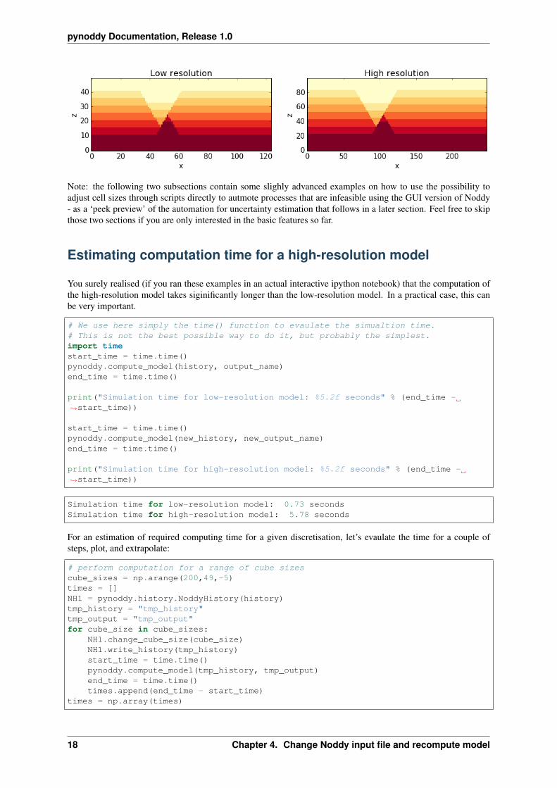
We can compare the effect of the different model discretisations in section plots, created with the plot_sectionmethod described before. Let’s get a bit more fancy here and use the functionality to pass axes to the plot_sectionmethod, and to create one figure as direct comparison:

# create basic figure layoutfig = plt.figure(figsize = (15,5))ax1 = fig.add_subplot(121)ax2 = fig.add_subplot(122)NO1.plot_section('y', position=0, ax = ax1, colorbar=False, title="Low resolution")NO2.plot_section('y', position=1, ax = ax2, colorbar=False, title="High resolution→˓")

plt.show()

4.2. Change model cube size and recompute model 17


Note: the following two subsections contain some slighly advanced examples on how to use the possibility toadjust cell sizes through scripts directly to autmote processes that are infeasible using the GUI version of Noddy- as a ‘peek preview’ of the automation for uncertainty estimation that follows in a later section. Feel free to skipthose two sections if you are only interested in the basic features so far.

Estimating computation time for a high-resolution model

You surely realised (if you ran these examples in an actual interactive ipython notebook) that the computation ofthe high-resolution model takes siginificantly longer than the low-resolution model. In a practical case, this canbe very important.

# We use here simply the time() function to evaulate the simualtion time.# This is not the best possible way to do it, but probably the simplest.import timestart_time = time.time()pynoddy.compute_model(history, output_name)end_time = time.time()

print("Simulation time for low-resolution model: %5.2f seconds" % (end_time -→˓start_time))

start_time = time.time()pynoddy.compute_model(new_history, new_output_name)end_time = time.time()

print("Simulation time for high-resolution model: %5.2f seconds" % (end_time -→˓start_time))

Simulation time for low-resolution model: 0.73 secondsSimulation time for high-resolution model: 5.78 seconds

For an estimation of required computing time for a given discretisation, let’s evaulate the time for a couple ofsteps, plot, and extrapolate:

# perform computation for a range of cube sizescube_sizes = np.arange(200,49,-5)times = []NH1 = pynoddy.history.NoddyHistory(history)tmp_history = "tmp_history"tmp_output = "tmp_output"for cube_size in cube_sizes:

NH1.change_cube_size(cube_size)NH1.write_history(tmp_history)start_time = time.time()pynoddy.compute_model(tmp_history, tmp_output)end_time = time.time()times.append(end_time - start_time)

times = np.array(times)



# create plotfig = plt.figure(figsize=(18,4))ax1 = fig.add_subplot(131)ax2 = fig.add_subplot(132)ax3 = fig.add_subplot(133)

ax1.plot(cube_sizes, np.array(times), 'ro-')ax1.set_xlabel('cubesize [m]')ax1.set_ylabel('time [s]')ax1.set_title('Computation time')ax1.set_xlim(ax1.get_xlim()[::-1])

ax2.plot(cube_sizes, times**(1/3.), 'bo-')ax2.set_xlabel('cubesize [m]')ax2.set_ylabel('(time [s])**(1/3)')ax2.set_title('Computation time (cuberoot)')ax2.set_xlim(ax2.get_xlim()[::-1])

ax3.semilogy(cube_sizes, times, 'go-')ax3.set_xlabel('cubesize [m]')ax3.set_ylabel('time [s]')ax3.set_title('Computation time (y-log)')ax3.set_xlim(ax3.get_xlim()[::-1])

(200.0, 40.0)

It is actually quite interesting that the computation time does not scale with cubesize to the power of three (ascould be expected, given that we have a mesh in three dimensions). Or am I missing something?

Anyway, just because we can: let’s assume that the scaling is somehow exponential and try to fit a model for atime prediction. Given the last plot, it looks like we could fit a logarithmic model with probably an additionalexponent (as the line is obviously not straight), so something like:

𝑓(𝑥) = 𝑎+ (𝑏 log10(𝑥))−𝑐

Let’s try to fit the curve with scipy.optimize.curve_fit:

# perform curve fitting with scipy.optimizeimport scipy.optimize# define function to be fitdef func(x,a,b,c):

return a + (b*np.log10(x))**(-c)

popt, pcov = scipy.optimize.curve_fit(func, cube_sizes, np.array(times), p0 = [-1,→˓0.5, 2])popt

array([ -0.05618538, 0.50990774, 12.45183398])

4.3. Estimating computation time for a high-resolution model 19


Interesting, it looks like Noody scales with something like:

𝑓(𝑥) = (0.5 log10(𝑥))−12

Note: if you understand more about computational complexity than me, it might not be that interesting to you atall - if this is the case, please contact me and tell me why this result could be expected...

a,b,c = poptcube_range = np.arange(200,20,-1)times_eval = func(cube_range, a, b, c)fig = plt.figure()ax = fig.add_subplot(111)ax.semilogy(cube_range, times_eval, '-')ax.semilogy(cube_sizes, times, 'ko')# reverse x-axisax.set_xlim(ax.get_xlim()[::-1])

(200.0, 20.0)

Not too bad... let’s evaluate the time for a cube size of 40 m:

cube_size = 40 # mtime_est = func(cube_size, a, b, c)print("Estimated time for a cube size of %d m: %.1f seconds" % (cube_size, time_→˓est))

Estimated time for a cube size of 40 m: 12.4 seconds

Now let’s check the actual simulation time:

NH1.change_cube_size(cube_size)NH1.write_history(tmp_history)start_time = time.time()pynoddy.compute_model(tmp_history, tmp_output)end_time = time.time()time_comp = end_time - start_time

print("Actual computation time for a cube size of %d m: %.1f seconds" % (cube_size,→˓ time_comp))



Actual computation time for a cube size of 40 m: 11.6 seconds

Not too bad, probably in the range of the inherent variability... and if we check it in the plot:

fig = plt.figure()ax = fig.add_subplot(111)ax.semilogy(cube_range, times_eval, '-')ax.semilogy(cube_sizes, times, 'ko')ax.semilogy(cube_size, time_comp, 'ro')# reverse x-axisax.set_xlim(ax.get_xlim()[::-1])

(200.0, 20.0)

Anyway, the point of this excercise was not a precise evaluation of Noddy’s computational complexity, but toprovide a simple means of evaluating computation time for a high resolution model, using the flexibility of writingsimple scripts using pynoddy, and a couple of additional python modules.

For a realistic case, it should, of course, be sufficient to determine the time based on a lot less computed points. Ifyou like, test it with your favourite model and tell me if it proved useful (or not)!

Simple convergence study

So: why would we want to run a high-resolution model, anyway? Well, of course, it produces nicer pictures - buton a scientific level, that’s completely irrelevant (haha, not true - so nice if it would be...).

Anyway, if we want to use the model in a scientific study, for example to evaluate volume of specific units, or toestimate the geological topology (Mark is working on this topic with some cool ideas - example to be implementedhere, “soon”), we want to know if the resolution of the model is actually high enough to produce meaningfulresults.

As a simple example of the evaluation of model resolution, we will here inlcude a volume convergence study,i.e. we will estimate at which level of increasing model resolution the estimated block volumes do not changeanymore.

4.4. Simple convergence study 21


The entire procedure is very similar to the computational time evaluation above, only that we now also analysethe output and determine the rock volumes of each defined geological unit:

# perform computation for a range of cube sizesreload(pynoddy.output)cube_sizes = np.arange(200,49,-5)all_volumes = []N_tmp = pynoddy.history.NoddyHistory(history)tmp_history = "tmp_history"tmp_output = "tmp_output"for cube_size in cube_sizes:

# adjust cube sizeN_tmp.change_cube_size(cube_size)N_tmp.write_history(tmp_history)pynoddy.compute_model(tmp_history, tmp_output)# open simulated model and determine volumesO_tmp = pynoddy.output.NoddyOutput(tmp_output)O_tmp.determine_unit_volumes()all_volumes.append(O_tmp.unit_volumes)

all_volumes = np.array(all_volumes)fig = plt.figure(figsize=(16,4))ax1 = fig.add_subplot(121)ax2 = fig.add_subplot(122)

# separate into two plots for better visibility:for i in range(np.shape(all_volumes)[1]):

if i < 4:ax1.plot(cube_sizes, all_volumes[:,i], 'o-', label='unit %d' %i)

else:ax2.plot(cube_sizes, all_volumes[:,i], 'o-', label='unit %d' %i)

ax1.legend(loc=2)ax2.legend(loc=2)# reverse axesax1.set_xlim(ax1.get_xlim()[::-1])ax2.set_xlim(ax2.get_xlim()[::-1])

ax1.set_xlabel("Block size [m]")ax1.set_ylabel("Total unit volume [m**3]")ax2.set_xlabel("Block size [m]")ax2.set_ylabel("Total unit volume [m**3]")

<matplotlib.text.Text at 0x107eb7250>

It looks like the volumes would start to converge from about a block size of 100 m. The example model is prettysmall and simple, probably not the best example for this study. Try it out with your own, highly complex, favouritepet model :-)


CHAPTER 5

Geological events in pynoddy: organisation and adpatiation

We will here describe how the single geological events of a Noddy history are organised within pynoddy. We willthen evaluate in some more detail how aspects of events can be adapted and their effect evaluated.


%matplotlib inline

Loading events from a Noddy history

In the current set-up of pynoddy, we always start with a pre-defined Noddy history loaded from a file, and thenchange aspects of the history and the single events. The first step is therefore to load the history file and to extractthe single geological events. This is done automatically as default when loading the history file into the Historyobject:

import sys, osimport matplotlib.pyplot as plt# adjust some settings for matplotlibfrom matplotlib import rcParams# print rcParamsrcParams['font.size'] = 15# determine path of repository to set paths corretly belowrepo_path = os.path.realpath('../..')

import pynoddyimport pynoddy.historyimport pynoddy.eventsimport pynoddy.outputreload(pynoddy)

<module 'pynoddy' from '/Users/flow/git/pynoddy/pynoddy/__init__.pyc'>


23


# Path to exmaple directory in this repositoryexample_directory = os.path.join(repo_path,'examples')# Compute noddy model for history filehistory = 'simple_two_faults.his'history_ori = os.path.join(example_directory, history)output_name = 'noddy_out'reload(pynoddy.history)reload(pynoddy.events)H1 = pynoddy.history.NoddyHistory(history_ori)# Before we do anything else, let's actually define the cube size here to# adjust the resolution for all subsequent examplesH1.change_cube_size(100)# compute model - note: not strictly required, here just to ensure changed cube→˓sizeH1.write_history(history)pynoddy.compute_model(history, output_name)

''

Events are stored in the object dictionary “events” (who would have thought), where the key corresponds to theposition in the timeline:

H1.events

{1: <pynoddy.events.Stratigraphy at 0x10cf2b410>,2: <pynoddy.events.Fault at 0x10cf2b450>,3: <pynoddy.events.Fault at 0x10cf2b490>}

We can see here that three events are defined in the history. Events are organised as objects themselves, containingall the relevant properties and information about the events. For example, the second fault event is defined as:

H1.events[3].properties

{'Amplitude': 2000.0,'Blue': 0.0,'Color Name': 'Custom Colour 5','Cyl Index': 0.0,'Dip': 60.0,'Dip Direction': 270.0,'Geometry': 'Translation','Green': 0.0,'Movement': 'Hanging Wall','Pitch': 90.0,'Profile Pitch': 90.0,'Radius': 1000.0,'Red': 254.0,'Rotation': 30.0,'Slip': 1000.0,'X': 5500.0,'XAxis': 2000.0,'Y': 7000.0,'YAxis': 2000.0,'Z': 5000.0,'ZAxis': 2000.0}

24 Chapter 5. Geological events in pynoddy: organisation and adpatiation


Changing aspects of geological events

So what we now want to do, of course, is to change aspects of these events and to evaluate the effect on theresulting geological model. Parameters can directly be updated in the properties dictionary:

H1 = pynoddy.history.NoddyHistory(history_ori)# get the original dip of the faultdip_ori = H1.events[3].properties['Dip']

# add 10 degrees to dipadd_dip = -10dip_new = dip_ori + add_dip

# and assign back to properties dictionary:H1.events[3].properties['Dip'] = dip_new# H1.events[2].properties['Dip'] = dip_new1

new_history = "dip_changed"new_output = "dip_changed_out"H1.write_history(new_history)pynoddy.compute_model(new_history, new_output)# load output from both modelsNO1 = pynoddy.output.NoddyOutput(output_name)NO2 = pynoddy.output.NoddyOutput(new_output)# create basic figure layoutfig = plt.figure(figsize = (15,5))ax1 = fig.add_subplot(121)ax2 = fig.add_subplot(122)NO1.plot_section('y', position=0, ax = ax1, colorbar=False, title="Dip = %.0f" %→˓dip_ori, savefig=True, fig_filename ="tmp.eps")NO2.plot_section('y', position=1, ax = ax2, colorbar=False, title="Dip = %.0f" %→˓dip_new)plt.show()

Changing the order of geological events

The geological history is parameterised as single events in a timeline. Changing the order of events can beperformed with two basic methods:

1. Swapping two events with a simple command

2. Adjusting the entire timeline with a complete remapping of events

The first method is probably the most useful to test how a simple change in the order of events will effect the finalgeological model. We will use it here with our example to test how the model would change if the timing of thefaults is swapped.

The method to swap two geological events is defined on the level of the history object:

5.2. Changing aspects of geological events 25


H1 = pynoddy.history.NoddyHistory(history_ori)

# The names of the two fault events defined in the history file are:print H1.events[2].nameprint H1.events[3].name

Fault2Fault1

We now swap the position of two events in the kinematic history. For this purpose, a high-level function candirectly be used:

# Now: swap the events:H1.swap_events(2,3)

# And let's check if this is correctly relfected in the events order now:print H1.events[2].nameprint H1.events[3].name

Fault1Fault2

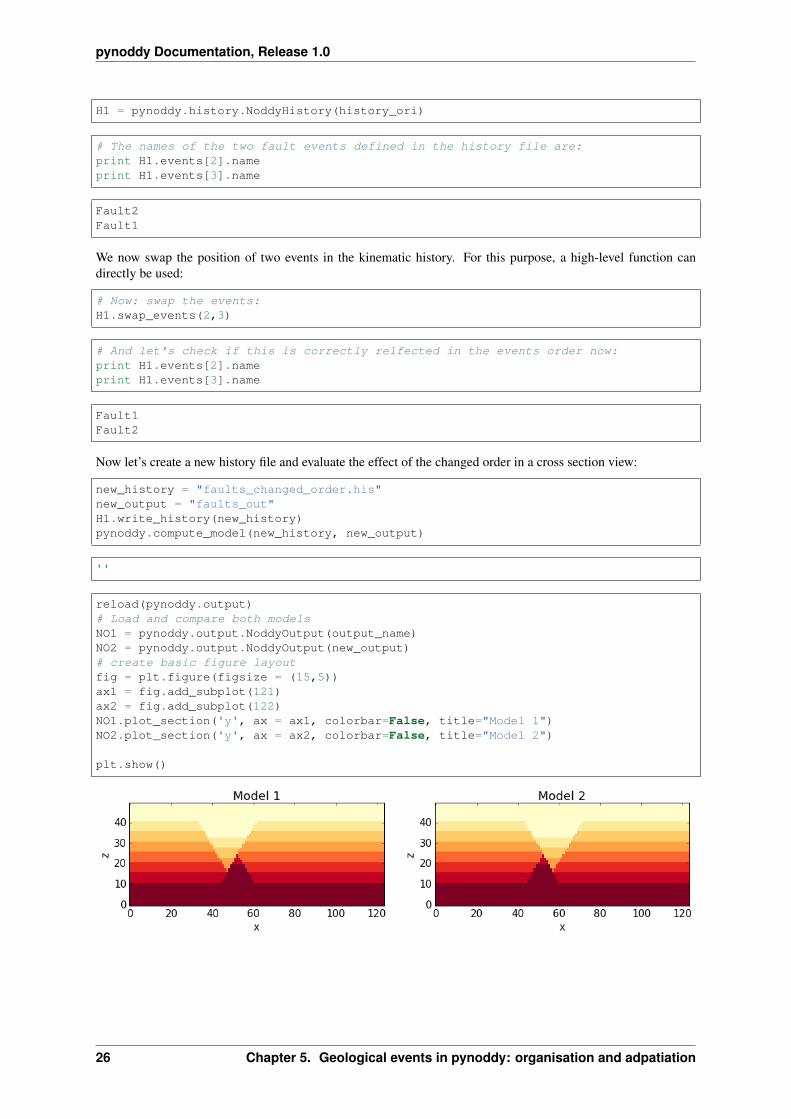
Now let’s create a new history file and evaluate the effect of the changed order in a cross section view:

new_history = "faults_changed_order.his"new_output = "faults_out"H1.write_history(new_history)pynoddy.compute_model(new_history, new_output)

''

reload(pynoddy.output)# Load and compare both modelsNO1 = pynoddy.output.NoddyOutput(output_name)NO2 = pynoddy.output.NoddyOutput(new_output)# create basic figure layoutfig = plt.figure(figsize = (15,5))ax1 = fig.add_subplot(121)ax2 = fig.add_subplot(122)NO1.plot_section('y', ax = ax1, colorbar=False, title="Model 1")NO2.plot_section('y', ax = ax2, colorbar=False, title="Model 2")

plt.show()



Determining the stratigraphic difference between two models

Just as another quick example of a possible application of pynoddy to evaluate aspects that are not simply possiblewith, for example, the GUI version of Noddy itself. In the last example with the changed order of the faults, wemight be interested to determine where in space this change had an effect. We can test this quite simply using theNoddyOutput objects.

The geology data is stored in the NoddyOutput.block attribute. To evaluate the difference between twomodels, we can therefore simply compute:

diff = (NO2.block - NO1.block)

And create a simple visualisation of the difference in a slice plot with:

fig = plt.figure(figsize = (5,3))ax = fig.add_subplot(111)ax.imshow(diff[:,10,:].transpose(), interpolation='nearest',

cmap = "RdBu", origin = 'lower left')

<matplotlib.image.AxesImage at 0x10cf3be10>

(Adding a meaningful title and axis labels to the plot is left to the reader as simple excercise :-) Future versions ofpynoddy might provide an automatic implementation for this step...)

Again, we may want to visualise results in 3-D. We can use the export_to_vtk-function as before, but nowassing the data array to be exported as the calulcated differnce field:

NO1.export_to_vtk(vtk_filename = "model_diff", data = diff)

A 3-D view of the difference plot is presented below.

5.4. Determining the stratigraphic difference between two models 27


Fig. 5.1: 3-D visualisation of stratigraphic id difference


CHAPTER 6

Creating a model from scratch

We describe here how to generate a simple history file for computation with Noddy using the functionality ofpynoddy. If possible, it is advisable to generate the history files with the Windows GUI for Noddy as this methodprovides, to date, a simpler and more complete interface to the entire functionality.

For completeness, pynoddy contains the functionality to generate simple models, for example to automate themodel construction process, or to enable the model construction for users who are not running Windows. Somesimple examlpes are shown in the following.

from matplotlib import rc_params


import sys, osimport matplotlib.pyplot as plt# adjust some settings for matplotlibfrom matplotlib import rcParams# print rcParamsrcParams['font.size'] = 15# determine path of repository to set paths corretly belowrepo_path = os.path.realpath('../..')import pynoddy.history

%matplotlib inline

rcParams.update({'font.size': 20})

Defining a stratigraphy

We start with the definition of a (base) stratigraphy for the model.

# Combined: model generation and output vis to test:history = "simple_model.his"output_name = "simple_out"

29


reload(pynoddy.history)reload(pynoddy.events)

# create pynoddy objectnm = pynoddy.history.NoddyHistory()# add stratigraphystrati_options = {'num_layers' : 8,

'layer_names' : ['layer 1', 'layer 2', 'layer 3','layer 4', 'layer 5', 'layer 6','layer 7', 'layer 8'],

'layer_thickness' : [1500, 500, 500, 500, 500, 500, 500, 500]}nm.add_event('stratigraphy', strati_options )

nm.write_history(history)

# Compute the modelreload(pynoddy)pynoddy.compute_model(history, output_name)

''

# Plot outputimport pynoddy.outputreload(pynoddy.output)nout = pynoddy.output.NoddyOutput(output_name)nout.plot_section('y', layer_labels = strati_options['layer_names'][::-1],

colorbar = True, title="",savefig = False, fig_filename = "ex01_strati.eps")

Add a fault event

As a next step, let’s now add the faults to the model.

reload(pynoddy.history)reload(pynoddy.events)nm = pynoddy.history.NoddyHistory()

30 Chapter 6. Creating a model from scratch


# add stratigraphystrati_options = {'num_layers' : 8,

'layer_names' : ['layer 1', 'layer 2', 'layer 3', 'layer 4',→˓'layer 5', 'layer 6', 'layer 7', 'layer 8'],


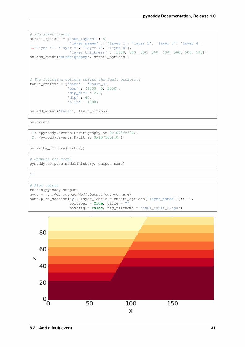
# The following options define the fault geometry:fault_options = {'name' : 'Fault_E',

'pos' : (6000, 0, 5000),'dip_dir' : 270,'dip' : 60,'slip' : 1000}

nm.add_event('fault', fault_options)

nm.events

{1: <pynoddy.events.Stratigraphy at 0x1073fc590>,2: <pynoddy.events.Fault at 0x107565fd0>}


# Compute the modelpynoddy.compute_model(history, output_name)

''

# Plot outputreload(pynoddy.output)nout = pynoddy.output.NoddyOutput(output_name)nout.plot_section('y', layer_labels = strati_options['layer_names'][::-1],

colorbar = True, title = "",savefig = False, fig_filename = "ex01_fault_E.eps")

6.2. Add a fault event 31


# The following options define the fault geometry:fault_options = {'name' : 'Fault_1',


nm.add_event('fault', fault_options)



''

# Plot outputreload(pynoddy.output)nout = pynoddy.output.NoddyOutput(output_name)nout.plot_section('y', layer_labels = strati_options['layer_names'][::-1],→˓colorbar = True)

nm1 = pynoddy.history.NoddyHistory(history)

nm1.get_extent()

(10000.0, 7000.0, 5000.0)

Complete Model Set-up

And here now, combining all the previous steps, the entire model set-up with base stratigraphy and two faults:



reload(pynoddy.history)reload(pynoddy.events)nm = pynoddy.history.NoddyHistory()# add stratigraphystrati_options = {'num_layers' : 8,

'layer_names' : ['layer 1', 'layer 2', 'layer 3','layer 4', 'layer 5', 'layer 6','layer 7', 'layer 8'],

'layer_thickness' : [1500, 500, 500, 500, 500,500, 500, 500]}

nm.add_event('stratigraphy', strati_options )

# The following options define the fault geometry:fault_options = {'name' : 'Fault_W',


nm.add_event('fault', fault_options)# The following options define the fault geometry:fault_options = {'name' : 'Fault_E',


nm.add_event('fault', fault_options)nm.write_history(history)

# Change cube sizenm1 = pynoddy.history.NoddyHistory(history)nm1.change_cube_size(50)nm1.write_history(history)


''

# Plot outputreload(pynoddy.output)nout = pynoddy.output.NoddyOutput(output_name)nout.plot_section('y', layer_labels = strati_options['layer_names'][::-1],

colorbar = True, title="",savefig = True, fig_filename = "ex01_faults_combined.eps",cmap = 'YlOrRd') # note: YlOrRd colourmap should be suitable for

→˓colorblindness!

6.3. Complete Model Set-up 33



CHAPTER 7

Read and Visualise Geophysical Potential-Fields

Geophysical potential fields (gravity and magnetics) can be calculated directly from the generated kinematicmodel. A wide range of options also exists to consider effects of geological events on the relevant rock prop-erties. We will here use pynoddy to simply and quickly test the effect of changing geological structures on thecalculated geophysical response.

%matplotlib inline

import sys, osimport matplotlib.pyplot as plt# adjust some settings for matplotlibfrom matplotlib import rcParams# print rcParamsrcParams['font.size'] = 15# determine path of repository to set paths corretly belowrepo_path = os.path.realpath('../..')import pynoddy

import matplotlib.pyplot as pltimport numpy as np


Read history file from Virtual Explorer

Many Noddy models are available on the site of the Virtual Explorer in the Structural Geophysics Atlas. We willdownload and use one of these models here as the base model.

We start with the history file of a “Fold and Thrust Belt” setting stored on:

http://tectonique.net/asg/ch3/ch3_5/his/fold_thrust.his

The file can directly be downloaded and opened with pynoddy:

35


import pynoddy.historyreload(pynoddy.history)

his = pynoddy.history.NoddyHistory(url = \"http://tectonique.net/asg/ch3/ch3_5/his/fold_thrust.his")

his.determine_model_stratigraphy()

his.change_cube_size(50)

# Save to (local) file to compute and visualise modelhistory_name = "fold_thrust.his"his.write_history(history_name)# his = pynoddy.history.NoddyHistory(history_name)

output = "fold_thrust_out"pynoddy.compute_model(history_name, output)

''

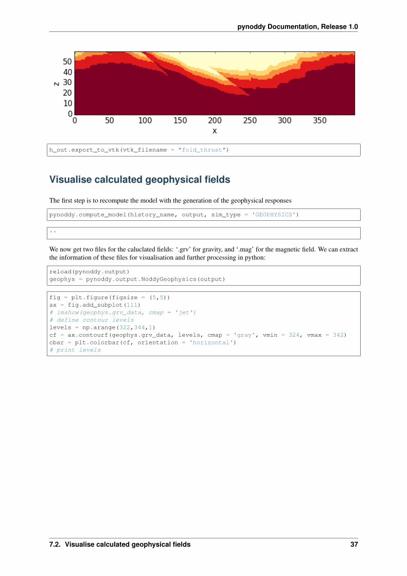
import pynoddy.output# load and visualise modelh_out = pynoddy.output.NoddyOutput(output)

# his.determine_model_stratigraphy()h_out.plot_section('x',

layer_labels = his.model_stratigraphy,colorbar_orientation = 'horizontal',colorbar=False,title = '',

# savefig=True, fig_filename = 'fold_thrust_NS_section.eps',cmap = 'YlOrRd')

h_out.plot_section('y', layer_labels = his.model_stratigraphy,colorbar_orientation = 'horizontal', title = '', cmap = 'YlOrRd

→˓',# savefig=True, fig_filename = 'fold_thrust_EW_section.eps',

ve=1.5)

36 Chapter 7. Read and Visualise Geophysical Potential-Fields


h_out.export_to_vtk(vtk_filename = "fold_thrust")

Visualise calculated geophysical fields

The first step is to recompute the model with the generation of the geophysical responses

pynoddy.compute_model(history_name, output, sim_type = 'GEOPHYSICS')

''

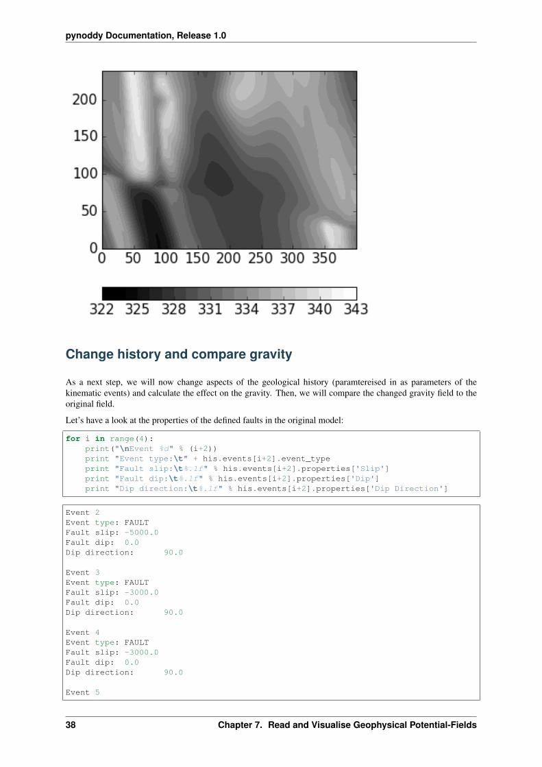
We now get two files for the caluclated fields: ‘.grv’ for gravity, and ‘.mag’ for the magnetic field. We can extractthe information of these files for visualisation and further processing in python:

reload(pynoddy.output)geophys = pynoddy.output.NoddyGeophysics(output)

fig = plt.figure(figsize = (5,5))ax = fig.add_subplot(111)# imshow(geophys.grv_data, cmap = 'jet')# define contour levelslevels = np.arange(322,344,1)cf = ax.contourf(geophys.grv_data, levels, cmap = 'gray', vmin = 324, vmax = 342)cbar = plt.colorbar(cf, orientation = 'horizontal')# print levels

7.2. Visualise calculated geophysical fields 37


Change history and compare gravity

As a next step, we will now change aspects of the geological history (paramtereised in as parameters of thekinematic events) and calculate the effect on the gravity. Then, we will compare the changed gravity field to theoriginal field.

Let’s have a look at the properties of the defined faults in the original model:

for i in range(4):print("\nEvent %d" % (i+2))print "Event type:\t" + his.events[i+2].event_typeprint "Fault slip:\t%.1f" % his.events[i+2].properties['Slip']print "Fault dip:\t%.1f" % his.events[i+2].properties['Dip']print "Dip direction:\t%.1f" % his.events[i+2].properties['Dip Direction']

Event 2Event type: FAULTFault slip: -5000.0Fault dip: 0.0Dip direction: 90.0



Event 5



Event type: FAULTFault slip: 12000.0Fault dip: 80.0Dip direction: 170.0

reload(pynoddy.history)reload(pynoddy.events)his2 = pynoddy.history.NoddyHistory("fold_thrust.his")

print his2.events[6].properties

{'Dip': 130.0, 'Cylindricity': 0.0, 'Wavelength': 12000.0, 'Amplitude': 1000.0,→˓'Pitch': 0.0, 'Y': 0.0, 'X': 0.0, 'Single Fold': 'FALSE', 'Z': 0.0, 'Type':→˓'Fourier', 'Dip Direction': 110.0}

As a simple test, we are changing the fault slip for all the faults and simply add 1000 m to all defined slips. Inorder to not mess up the original model, we are creating a copy of the history object first:

import copyhis = pynoddy.history.NoddyHistory(history_name)his.all_events_end += 1his_changed = copy.deepcopy(his)

# change parameters of kinematic eventsslip_change = 2000.wavelength_change = 2000.# his_changed.events[3].properties['Slip'] += slip_change# his_changed.events[5].properties['Slip'] += slip_change# change fold wavelengthhis_changed.events[6].properties['Wavelength'] += wavelength_changehis_changed.events[6].properties['X'] += wavelength_change/2.

We now write the adjusted history back to a new history file and then calculate the updated gravity field:

his_changed.write_history('fold_thrust_changed.his')

# %%timeit# recompute block modelpynoddy.compute_model('fold_thrust_changed.his', 'fold_thrust_changed_out')

''

# %%timeit# recompute geophysical responsepynoddy.compute_model('fold_thrust_changed.his', 'fold_thrust_changed_out',

sim_type = 'GEOPHYSICS')

''

# load changed block modelgeo_changed = pynoddy.output.NoddyOutput('fold_thrust_changed_out')# load output and visualise geophysical fieldgeophys_changed = pynoddy.output.NoddyGeophysics('fold_thrust_changed_out')

fig = plt.figure(figsize = (5,5))ax = fig.add_subplot(111)# imshow(geophys_changed.grv_data, cmap = 'jet')cf = ax.contourf(geophys_changed.grv_data, levels, cmap = 'gray', vmin = 324, vmax→˓= 342)cbar = plt.colorbar(cf, orientation = 'horizontal')

7.3. Change history and compare gravity 39


fig = plt.figure(figsize = (5,5))ax = fig.add_subplot(111)# imshow(geophys.grv_data - geophys_changed.grv_data, cmap = 'jet')maxval = np.ceil(np.max(np.abs(geophys.grv_data - geophys_changed.grv_data)))# comp_levels = np.arange(-maxval,1.01 * maxval, 0.05 * maxval)cf = ax.contourf(geophys.grv_data - geophys_changed.grv_data, 20,

cmap = 'spectral')cbar = plt.colorbar(cf, orientation = 'horizontal')



# compare sections through modelgeo_changed.plot_section('y', colorbar = False)h_out.plot_section('y', colorbar = False)

for i in range(4):print("Event %d" % (i+2))print his.events[i+2].properties['Slip']print his.events[i+2].properties['Dip']print his.events[i+2].properties['Dip Direction']

Event 2-5000.00.090.0Event 3-3000.00.090.0Event 4-3000.00.090.0Event 512000.080.0170.0

# recompute the geology blocks for comparison:pynoddy.compute_model('fold_thrust_changed.his', 'fold_thrust_changed_out')

''

geology_changed = pynoddy.output.NoddyOutput('fold_thrust_changed_out')

geology_changed.plot_section('x',# layer_labels = his.model_stratigraphy,

colorbar_orientation = 'horizontal',colorbar=False,

7.3. Change history and compare gravity 41


title = '',# savefig=True, fig_filename = 'fold_thrust_NS_section.eps',

cmap = 'YlOrRd')

geology_changed.plot_section('y',# layer_labels = his.model_stratigraphy,

colorbar_orientation = 'horizontal', title = '', cmap = 'YlOrRd→˓',# savefig=True, fig_filename = 'fold_thrust_EW_section.eps',

ve=1.5)

# Calculate block difference and export as VTK for 3-D visualisation:import copydiff_model = copy.deepcopy(geology_changed)diff_model.block -= h_out.block

diff_model.export_to_vtk(vtk_filename = "diff_model_fold_thrust_belt")

Figure with all results

We now create a figure with the gravity field of the original and the changed model, as well as a difference plotto highlight areas with significant changes. This example also shows how additional equations can easily becombined with pynoddy classes.

fig = plt.figure(figsize=(20,8))ax1 = fig.add_subplot(131)# original plotlevels = np.arange(322,344,1)cf1 = ax1.contourf(geophys.grv_data, levels, cmap = 'gray', vmin = 324, vmax = 342)# cbar1 = ax1.colorbar(cf1, orientation = 'horizontal')fig.colorbar(cf1, orientation='horizontal')ax1.set_title('Gravity of original model')



ax2 = fig.add_subplot(132)

cf2 = ax2.contourf(geophys_changed.grv_data, levels, cmap = 'gray', vmin = 324,→˓vmax = 342)ax2.set_title('Gravity of changed model')fig.colorbar(cf2, orientation='horizontal')

ax3 = fig.add_subplot(133)

comp_levels = np.arange(-10.,10.1,0.25)cf3 = ax3.contourf(geophys.grv_data - geophys_changed.grv_data, comp_levels, cmap→˓= 'RdBu_r')ax3.set_title('Gravity difference')

fig.colorbar(cf3, orientation='horizontal')

plt.savefig("grav_ori_changed_compared.eps")

7.4. Figure with all results 43



CHAPTER 8

Reproducible Experiments with pynoddy

All pynoddy experiments can be defined in a Python script, and if all settings are appropriate, then this script canbe re-run to obtain a reproduction of the results. However, it is often more convenient to encapsulate all elements ofan experiment within one class. We show here how this is done in the pynoddy.experiment.Experimentclass and how this class can be used to define simple reproducible experiments with kinematic models.


%matplotlib inline

# here the usual imports. If any of the imports fails,# make sure that pynoddy is installed# properly, ideally with 'python setup.py develop'# or 'python setup.py install'import sys, osimport matplotlib.pyplot as pltimport numpy as np# adjust some settings for matplotlibfrom matplotlib import rcParams# print rcParamsrcParams['font.size'] = 15# determine path of repository to set paths corretly belowrepo_path = os.path.realpath('../..')import pynoddy.historyimport pynoddy.experimentreload(pynoddy.experiment)rcParams.update({'font.size': 15})

Defining an experiment

We are considering the following scenario: we defined a kinematic model of a prospective geological unit at depth.As we know that the estimates of the (kinematic) model parameters contain a high degree of uncertainty, we wouldlike to represent this uncertainty with the model.

45


Our approach is here to perform a randomised uncertainty propagation analysis with a Monte Carlo samplingmethod. Results should be presented in several figures (2-D slice plots and a VTK representation in 3-D).

To perform this analysis, we need to perform the following steps (see main paper for more details):

1. Define kinematic model parameters and construct the initial (base) model;

2. Assign probability distributions (and possible parameter correlations) to relevant uncertain input parameters;

3. Generate a set of n random realisations, repeating the following steps:

(a) Draw a randomised input parameter set from the parameter distribution;

(b) Generate a model with this parameter set;

(c) Analyse the generated model and store results;

4. Finally: perform postprocessing, generate figures of results

It would be possible to write a Python script to perform all of these steps in one go. However, we will here takeanother path and use the implementation in a Pynoddy Experiment class. Initially, this requires more work anda careful definition of the experiment - but, finally, it will enable a higher level of flexibility, extensibility, andreproducibility.

Loading an example model from the Atlas of Structural Geophysics

As in the example for geophysical potential-field simulation, we will use a model from the Atlas of StructuralGeophysics as an examlpe model for this simulation. We use a model for a fold interference structure. A discre-tised 3-D version of this model is presented in the figure below. The model represents a fold interference patternof “Type 1” according to the definition of Ramsey (1967).

Fig. 8.1: Fold interference pattern

Instead of loading the model into a history object, we are now directly creating an experiment object:

46 Chapter 8. Reproducible Experiments with pynoddy


reload(pynoddy.history)reload(pynoddy.experiment)

from pynoddy.experiment import monte_carlomodel_url = 'http://tectonique.net/asg/ch3/ch3_7/his/typeb.his'ue = pynoddy.experiment.Experiment(url = model_url)

For simpler visualisation in this notebook, we will analyse the following steps in a section view of the model.

We consider a section in y-direction through the model:

ue.write_history("typeb_tmp3.his")

ue.write_history("typeb_tmp2.his")

ue.change_cube_size(100)ue.plot_section('y')

Before we start to draw random realisations of the model, we should first store the base state of the model forlater reference. This is simply possibel with the freeze() method which stores the current state of the model as the“base-state”:

ue.freeze()

We now intialise the random generator. We can directly assign a random seed to simplify reproducibility (notethat this is not essential, as it would be for the definition in a script function: the random state is preserved withinthe model and could be retrieved at a later stage, as well!):

ue.set_random_seed(12345)

The next step is to define probability distributions to the relevant event parameters. Let’s first look at the differentevents:

ue.info(events_only = True)

This model consists of 3 events:(1) - STRATIGRAPHY(2) - FOLD(3) - FOLD

8.2. Loading an example model from the Atlas of Structural Geophysics 47


ev2 = ue.events[2]

ev2.properties

{'Amplitude': 1250.0,'Cylindricity': 0.0,'Dip': 90.0,'Dip Direction': 90.0,'Pitch': 0.0,'Single Fold': 'FALSE','Type': 'Sine','Wavelength': 5000.0,'X': 1000.0,'Y': 0.0,'Z': 0.0}

Next, we define the probability distributions for the uncertain input parameters:

param_stats = [{'event' : 2,'parameter': 'Amplitude','stdev': 100.0,'type': 'normal'},{'event' : 2,'parameter': 'Wavelength','stdev': 500.0,'type': 'normal'},{'event' : 2,'parameter': 'X','stdev': 500.0,'type': 'normal'}]

ue.set_parameter_statistics(param_stats)

resolution = 100ue.change_cube_size(resolution)tmp = ue.get_section('y')prob_4 = np.zeros_like(tmp.block[:,:,:])n_draws = 100

for i in range(n_draws):ue.random_draw()tmp = ue.get_section('y', resolution = resolution)prob_4 += (tmp.block[:,:,:] == 4)

# Normaliseprob_4 = prob_4 / float(n_draws)

fig = plt.figure(figsize = (12,8))ax = fig.add_subplot(111)ax.imshow(prob_4.transpose()[:,0,:],

origin = 'lower left',interpolation = 'none')

plt.title("Estimated probability of unit 4")plt.xlabel("x (E-W)")plt.ylabel("z")

<matplotlib.text.Text at 0x10ba80250>



This example shows how the base module for reproducible experiments with kinematics can be used. For furtherspecification, child classes of Experiment can be defined, and we show examples of this type of extension inthe next sections.

8.2. Loading an example model from the Atlas of Structural Geophysics 49



CHAPTER 9

Gippsland Basin Uncertainty Study


%matplotlib inline

#import the ususal libraries + the pynoddy UncertaintyAnalysis class

import sys, os, pynoddy# from pynoddy.experiment.UncertaintyAnalysis import UncertaintyAnalysis

# adjust some settings for matplotlibfrom matplotlib import rcParams# print rcParamsrcParams['font.size'] = 15

# determine path of repository to set paths corretly belowrepo_path = os.path.realpath('../..')import pynoddy.historyimport pynoddy.experiment.uncertainty_analysisrcParams.update({'font.size': 20})

The Gippsland Basin Model

In this example we will apply the UncertaintyAnalysis class we have been playing with in the previous example to a‘realistic’ (though highly simplified) geological model of the Gippsland Basin, a petroleum field south of Victoria,Australia. The model has been included as part of the PyNoddy directory, and can be found at pynoddy/examples/GBasin_Ve1_V4.his

reload(pynoddy.history)reload(pynoddy.output)reload(pynoddy.experiment.uncertainty_analysis)reload(pynoddy)

# the model itself is now part of the repository, in the examples directory:history_file = os.path.join(repo_path, "examples/GBasin_Ve1_V4.his")

51


While we could hard-code parameter variations here, it is much easier to store our statistical information in a csvfile, so we load that instead. This file accompanies the GBasin_Ve1_V4 model in the pynoddy directory.

params = os.path.join(repo_path,"examples/gipps_params.csv")

Generate randomised model realisations

Now we have all the information required to perform a Monte-Carlo based uncertainty analysis. In this example wewill generate 100 model realisations and use them to estimate the information entropy of each voxel in the model,and hence visualise uncertainty. It is worth noting that in reality we would need to produce several thousandmodel realisations in order to adequately sample the model space, however for convinience we only generate asmall number of models here.

# %%timeit # Uncomment to test execution timeua = pynoddy.experiment.uncertainty_analysis.UncertaintyAnalysis(history_file,→˓params)ua.estimate_uncertainty(100,verbose=False)

A few utility functions for visualising uncertainty have been included in the UncertaintyAnalysis class, and canbe used to gain an understanding of the most uncertain parts of the Gippsland Basin. The probabability voxetsfor each lithology can also be accessed using ua.p_block[lithology_id], and the information entropyvoxset accessed using ua.e_block.

Note that the Gippsland Basin model has been computed with a vertical exaggeration of 3, in order to highlightvertical structure.

ua.plot_section(direction='x',data=ua.block)ua.plot_entropy(direction='x')

It is immediately apparent (and not particularly surprising) that uncertainty in the Gippsland Basin model isconcentrated around the thin (but economically interesting) formations comprising the La Trobe and Strzelecki

52 Chapter 9. Gippsland Basin Uncertainty Study


Groups. The faults in the model also contribute to this uncertainty, though not by a huge amount.

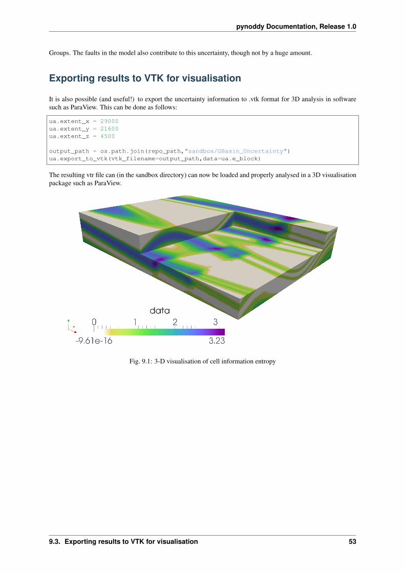
Exporting results to VTK for visualisation

It is also possible (and useful!) to export the uncertainty information to .vtk format for 3D analysis in softwaresuch as ParaView. This can be done as follows:

ua.extent_x = 29000ua.extent_y = 21600ua.extent_z = 4500

output_path = os.path.join(repo_path,"sandbox/GBasin_Uncertainty")ua.export_to_vtk(vtk_filename=output_path,data=ua.e_block)

The resulting vtr file can (in the sandbox directory) can now be loaded and properly analysed in a 3D visualisationpackage such as ParaView.

Fig. 9.1: 3-D visualisation of cell information entropy

9.3. Exporting results to VTK for visualisation 53


54 Chapter 9. Gippsland Basin Uncertainty Study

CHAPTER 10

Sensitivity Analysis

Test here: (local) sensitivity analysis of kinematic parameters with respect to a defined objective function. Aim:test how sensitivity the resulting model is to uncertainties in kinematic parameters to:

1. Evaluate which the most important parameters are, and to

2. Determine which parameters could, in principle, be inverted with suitable information.

Theory: local sensitivity analysis

Basic considerations:

• parameter vector 𝑝

• residual vector �⃗�

• calculated values at observation points �⃗�

• Jacobian matrix 𝐽𝑖𝑗 =𝜕�⃗�𝜕𝑝

Numerical estimation of Jacobian matrix with central difference scheme (see Finsterle):

𝐽𝑖𝑗 =𝜕𝑧𝑖𝜕𝑝𝑗

≈ 𝑧𝑖(𝑝; 𝑝𝑗 + 𝛿𝑝𝑗)− 𝑧𝑖(𝑝; 𝑝𝑗 − 𝛿𝑝𝑗)

2𝛿𝑝𝑗

where 𝛿𝑝𝑗 is a small perturbation of parameter 𝑗, often as a fraction of the value.

Defining the responses

A meaningful sensitivity analysis obviously depends on the definition of a suitable response vector �⃗�. Ideally,these responses are related to actual observations. In our case, we first want to determine how sensitive a kine-matic structural geological model is with respect to uncertainties in the kinematic parameters. We therefore needcalculatable measures that describe variations of the model.

As a first-order assumption, we will use a notation of a stratigraphic distance for discrete subsections of themodel, for example in single voxets for the calculated model. We define distance 𝑑 of a subset 𝜔 as the (discrete)difference between the (discrete) stratigraphic value of an ideal model, 𝑠, to the value of a model realisation 𝑠𝑖:

𝑑(𝜔) = 𝑠− 𝑠𝑖

55


In the first example, we will consider only one response: the overall sum of stratigraphic distances for a modelrealisation 𝑟 of all subsets (= voxets, in the practical sense), scaled by the number of subsets (for a subsequentcomparison of model discretisations):

𝐷𝑟 =1

𝑛

𝑛∑︁𝑖=1

𝑑(𝜔𝑖)

Note: mistake before: not considering distances at single nodes but only the sum - this lead to “zero-difference”for simple translation! Now: consider more realistic objective function, squared distance:

𝑟 =

√︃∑︁𝑖

(𝑧𝑖𝑐𝑎𝑙𝑐 − 𝑧𝑖𝑟𝑒𝑓 )2


%matplotlib inline

Setting up the base model

For a first test: use simple two-fault model from paper

import sys, osimport matplotlib.pyplot as pltimport numpy as np# adjust some settings for matplotlibfrom matplotlib import rcParams# print rcParamsrcParams['font.size'] = 15# determine path of repository to set paths corretly belowrepo_path = os.path.realpath('../..')import pynoddy.historyimport pynoddy.eventsimport pynoddy.output




# The following options define the fault geometry:fault_options = {'name' : 'Fault_W',


nm.add_event('fault', fault_options)# The following options define the fault geometry:fault_options = {'name' : 'Fault_E',

'pos' : (6000, 3500, 5000),'dip_dir' : 270,

56 Chapter 10. Sensitivity Analysis


'dip' : 60,'slip' : 1000}

nm.add_event('fault', fault_options)history = "two_faults_sensi.his"nm.write_history(history)

output_name = "two_faults_sensi_out"# Compute the modelpynoddy.compute_model(history, output_name)

''

# Plot outputnout = pynoddy.output.NoddyOutput(output_name)nout.plot_section('y', layer_labels = strati_options['layer_names'][::-1],

colorbar = True, title="",savefig = False)

Define parameter uncertainties

We will start with a sensitivity analysis for the parameters of the fault events.

H1 = pynoddy.history.NoddyHistory(history)# get the original dip of the faultdip_ori = H1.events[3].properties['Dip']# dip_ori1 = H1.events[2].properties['Dip']# add 10 degrees to dipadd_dip = -20dip_new = dip_ori + add_dip# dip_new1 = dip_ori1 + add_dip

# and assign back to properties dictionary:H1.events[3].properties['Dip'] = dip_new

10.4. Define parameter uncertainties 57


reload(pynoddy.output)new_history = "sensi_test_dip_changed.his"new_output = "sensi_test_dip_changed_out"H1.write_history(new_history)pynoddy.compute_model(new_history, new_output)# load output from both modelsNO1 = pynoddy.output.NoddyOutput(output_name)NO2 = pynoddy.output.NoddyOutput(new_output)

# create basic figure layoutfig = plt.figure(figsize = (15,5))ax1 = fig.add_subplot(121)ax2 = fig.add_subplot(122)NO1.plot_section('y', position=0, ax = ax1, colorbar=False, title="Dip = %.0f" %→˓dip_ori)NO2.plot_section('y', position=0, ax = ax2, colorbar=False, title="Dip = %.0f" %→˓dip_new)

plt.show()

Calculate total stratigraphic distance

# def determine_strati_diff(NO1, NO2):# """calculate total stratigraphic distance between two models"""# return np.sum(NO1.block - NO2.block) / float(len(NO1.block))

def determine_strati_diff(NO1, NO2):"""calculate total stratigraphic distance between two models"""return np.sqrt(np.sum((NO1.block - NO2.block)**2)) / float(len(NO1.block))

diff = determine_strati_diff(NO1, NO2)print(diff)

5.56205897128

Function to modify parameters

Multiple event parameters can be changed directly with the function change_event_params, which takesa dictionarly of events and parameters with according changes relative to the defined parameters. Here a briefexample:



# set parameter changes in dictionary

changes_fault_1 = {'Dip' : -20}changes_fault_2 = {'Dip' : -20}param_changes = {2 : changes_fault_1,

3 : changes_fault_2}

reload(pynoddy.history)H2 = pynoddy.history.NoddyHistory(history)H2.change_event_params(param_changes)

new_history = "param_dict_changes.his"new_output = "param_dict_changes_out"H2.write_history(new_history)pynoddy.compute_model(new_history, new_output)# load output from both modelsNO1 = pynoddy.output.NoddyOutput(output_name)NO2 = pynoddy.output.NoddyOutput(new_output)

# create basic figure layoutfig = plt.figure(figsize = (15,5))ax1 = fig.add_subplot(121)ax2 = fig.add_subplot(122)NO1.plot_section('y', position=0, ax = ax1, colorbar=False, title="Original Model")NO2.plot_section('y', position=0, ax = ax2, colorbar=False, title="Changed Model")

plt.show()

Full sensitivity analysis

Perform now a full sensitivity analysis for all defined parameters and analyse the output matrix. For a betteroverview, we first create a function to perform the sensitivity analysis:

import copynew_history = "sensi_tmp.his"new_output = "sensi_out"def noddy_sensitivity(history_filename, param_change_vals):

"""Perform noddy sensitivity analysis for a model"""param_list = [] # list to store parameters for later analysisdistances = [] # list to store calcualted distances# Step 1:# create new parameter list to change modelfor event_id, event_dict in param_change_vals.items(): # iterate over events

for key, val in event_dict.items(): # iterate over all properties→˓separately

changes_list = dict()

10.7. Full sensitivity analysis 59


changes_list[event_id] = dict()param_list.append("event_%d_property_%s" % (event_id, key))for i in range(2):

# calculate positive and negative valueshis = pynoddy.history.NoddyHistory(history_filename)if i == 0:

changes_list[event_id][key] = val# set changeshis.change_event_params(changes_list)# save and calculate modelhis.write_history(new_history)pynoddy.compute_model(new_history, new_output)# open output and calculate distanceNO_tmp = pynoddy.output.NoddyOutput(new_output)dist_pos = determine_strati_diff(NO1, NO_tmp)NO_tmp.plot_section('y', position = 0, colorbar = False,

title = "Dist: %.2f" % dist_pos,savefig = True,fig_filename = "event_%d_property_%s_val_

→˓%d.png" \% (event_id, key,val))

if i == 1:changes_list[event_id][key] = -valhis.change_event_params(changes_list)# save and calculate modelhis.write_history(new_history)pynoddy.compute_model(new_history, new_output)# open output and calculate distanceNO_tmp = pynoddy.output.NoddyOutput(new_output)dist_neg = determine_strati_diff(NO1, NO_tmp)NO_tmp.plot_section('y', position=0, colorbar=False,

title="Dist: %.2f" % dist_neg,savefig=True,fig_filename="event_%d_property_%s_val_%d.

→˓png" \% (event_id, key,val))

# calculate central differencecentral_diff = (dist_pos + dist_neg) / (2.)distances.append(central_diff)

return param_list, distances

As a next step, we define the parameter ranges for the local sensitivity analysis (i.e. the 𝛿𝑝𝑗 from the theoreticaldescription above):

changes_fault_1 = {'Dip' : 1.5,'Dip Direction' : 10,'Slip': 100.0,'X': 500.0}

changes_fault_2 = {'Dip' : 1.5,'Dip Direction' : 10,'Slip': 100.0,'X': 500.0}

param_changes = {2 : changes_fault_1,3 : changes_fault_2}

And now, we perform the local sensitivity analysis:

param_list_1, distances = noddy_sensitivity(history, param_changes)

The function passes back a list of the changed parameters and the calculated distances according to this change.Let’s have a look at the results:



for p,d in zip(param_list_1, distances):print "%s \t\t %f" % (p, d)

event_2_property_X 2.716228event_2_property_Dip 1.410039event_2_property_Dip Direction 2.133553event_2_property_Slip 1.824993event_3_property_X 3.323528event_3_property_Dip 1.644589event_3_property_Dip Direction 2.606573event_3_property_Slip 1.930455

Results of this local sensitivity analysis suggest that the model is most sensitive to the X-position of the fault,when we evaluate distances as simple stratigraphic id differences. Here just a bar plot for better visualisation (feelfree to add proper labels):

d = np.array([distances])fig = plt.figure(figsize=(5,3))ax = fig.add_subplot(111)ax.bar(np.arange(0.6,len(distances),1.), np.array(distances[:]))

<Container object of 8 artists>

The previous experiment showed how pynoddy can be used for simple scientific experiments. The sensitivityanalysis itself is purely local. A better way would be to use (more) global sensitivity analysis, for exampleusing the Morris or Sobol methods. These methods are implemented in the Python package SALib, and anexperimental implementation of this method into pynoddy exists, as well (see further notebooks on repository,note: no guaranteed working, so far!).

10.7. Full sensitivity analysis 61



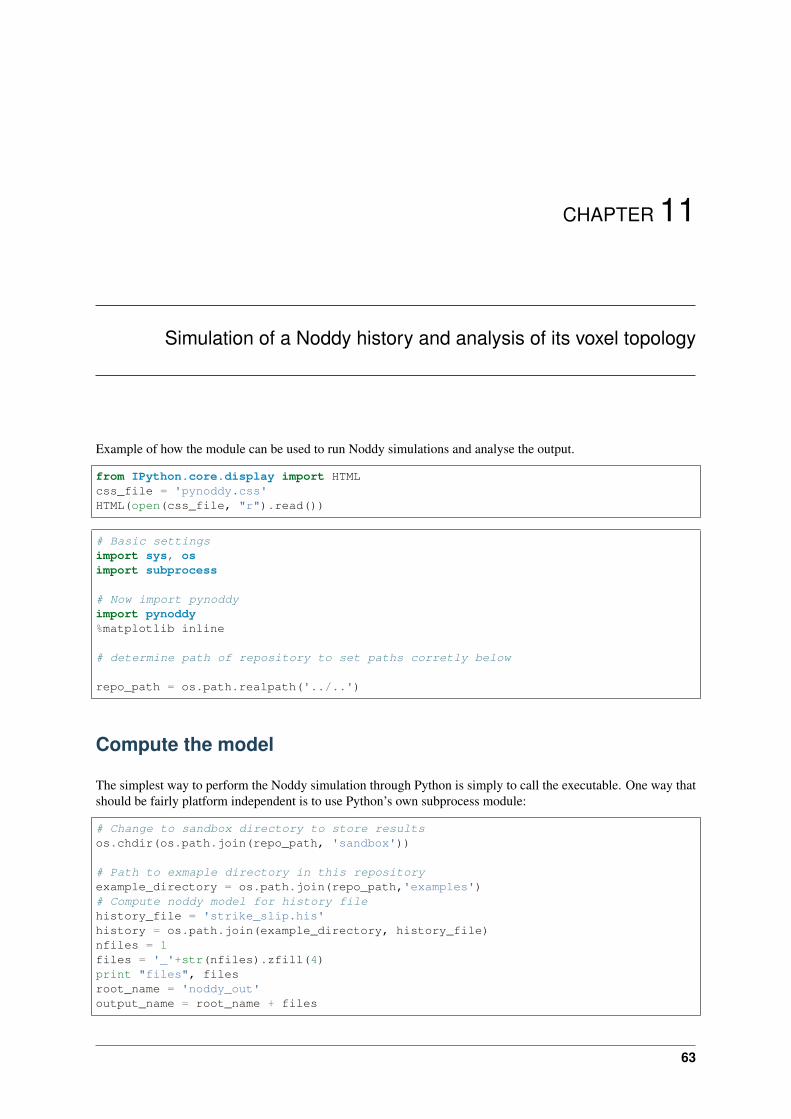
CHAPTER 11

Simulation of a Noddy history and analysis of its voxel topology

Example of how the module can be used to run Noddy simulations and analyse the output.


# Basic settingsimport sys, osimport subprocess

# Now import pynoddyimport pynoddy%matplotlib inline

# determine path of repository to set paths corretly below

repo_path = os.path.realpath('../..')

Compute the model

The simplest way to perform the Noddy simulation through Python is simply to call the executable. One way thatshould be fairly platform independent is to use Python’s own subprocess module:


# Path to exmaple directory in this repositoryexample_directory = os.path.join(repo_path,'examples')# Compute noddy model for history filehistory_file = 'strike_slip.his'history = os.path.join(example_directory, history_file)nfiles = 1files = '_'+str(nfiles).zfill(4)print "files", filesroot_name = 'noddy_out'output_name = root_name + files

63


print root_nameprint output_name# call Noddy

# NOTE: Make sure that the noddy executable is accessible in the system!!sysprint subprocess.Popen(['noddy.exe', history, output_name, 'TOPOLOGY'],


#sysprint subprocess.Popen(['topology.exe', root_name, files],


files _0001noddy_outnoddy_out_0001

For convenience, the model computations are wrapped into a Python function in pynoddy:

pynoddy.compute_model(history, output_name)pynoddy.compute_topology(root_name, files)

Note: The Noddy call from Python is, to date, calling Noddy through the subprocess function. In a future im-plementation, this call could be subsituted with a full wrapper for the C-functions written in Python. Therefore,using the member function compute_model is not only easier, but also the more “future-proof” way to computethe Noddy model.

Loading Topology output files

Here we load the binary adjacency matrix for one topology calculation and display it as an image

from matplotlib import pyplot as pltimport matplotlib.image as mpimgimport numpy as np

N1 = pynoddy.NoddyOutput(output_name)AM= pynoddy.NoddyTopology(output_name)

am_name=root_name +'_uam.bin'print am_nameprint AM.maxlitho

image = np.empty((int(AM.maxlitho),int(AM.maxlitho)), np.uint8)

image.data[:] = open(am_name).read()cmap=plt.get_cmap('Paired')cmap.set_under('white') # Color for values less than vmin

plt.imshow(image, interpolation="nearest", vmin=1, cmap=cmap)plt.show()

maxlitho = 7

noddy_out_uam.bin7

64 Chapter 11. Simulation of a Noddy history and analysis of its voxel topology


11.2. Loading Topology output files 65


66 Chapter 11. Simulation of a Noddy history and analysis of its voxel topology

CHAPTER 12

Fault shapes

We are here briefly showing the possibility of Noddy to model more complex fault shapes than simple planarfaults.

from matplotlib import rc_params


import sys, osimport matplotlib.pyplot as plt# adjust some settings for matplotlibfrom matplotlib import rcParams# print rcParamsrcParams['font.size'] = 15# determine path of repository to set paths corretly belowrepo_path = os.path.realpath('../..')import pynoddy.historyimport pynoddy.experimentimport pynoddy.events

<module 'pynoddy.experiment' from '/Users/flow/git/pynoddy/pynoddy/experiment/__→˓init__.pyc'>

%matplotlib inline

rcParams.update({'font.size': 20})

We will create a model with a listric fault from scratch. In addition to the previous parameters for creating a fault(see notebook 4-Create-model), we now change the fault “geometry” to “Curved” and add parameters defining theamplitude and radius of influence:


67




# The following options define the fault geometry:fault_options = {'name' : 'Fault_E',

'pos' : (3000, 0, 4000),'dip_dir' : 90,'dip' : 30,'slip' : 1000,'amplitude' : 1000.,'radius' : 2000,

'geometry' : 'Curved','xaxis': 5000.,'yaxis': 5000.0,

'zaxis' : 39999.0}nm.add_event('fault', fault_options)nm.change_cube_size(50)

With these settings, we obtain an example of a listric fault in Noddy:

history = "listric_example.his"outout_name = "listric_out"

nm.write_history(history)# Compute the modelpynoddy.compute_model(history, output_name)# Plot outputreload(pynoddy.output)nout = pynoddy.output.NoddyOutput(output_name)nout.plot_section('y', layer_labels = strati_options['layer_names'][::-1],

colorbar = True, title = "",savefig = False, fig_filename = "ex01_fault_listric.eps")

68 Chapter 12. Fault shapes

CHAPTER 13

Pynoddy modules, classes and functions

Basic modules (low-level access)

The modules in this section provide low-level access to the functionality in Noddy. Basically, these modulesprovide parsers for Noddy input and output files and class definitions for suitable Noddy elements.

Main module

History file parser: pynoddy.history

Output file parser: pynoddy.output

Additional useful classes

pynoddy.events

Modules for Kinematic experiments

The modules described in this section are designed to provide a high-level access to the kinematic modellingfunctionality in Noddy. The modules encapsulate the required aspects of complete experiments, including inputfile generation, adaptation of parameters, random number generation, model computation, and postprocessing.

Base classes for pynoddy experiments

The base class for any type of experiments is defined in the pynoddy.experiment module.

MonteCarlo class

This class provides the basic functionality to perform MonteCarlo error propagation experiments with Noddy.

SensitivityAnalysis class

69

Documents

Release 1.0 Florian Wellmann, Sam Thiele · 3.2 Loading Noddy output ﬁles. . . . . . . . . . . . . . . . . . . . . . . . . . . . . . . . . . . . .12