Embed Size (px)
Citation preview

Reliability and Survivial Analysis


Table Of Contents
Copyright © 2003–2005 Minitab Inc. All rights reserved. 3
Table Of Contents Test Plans .............................................................................................................................................................................. 7
Test Plans Overview......................................................................................................................................................... 7 Failure Censoring ............................................................................................................................................................. 7 Time Censoring ................................................................................................................................................................ 8 Type I and Type II Errors.................................................................................................................................................. 8 Demonstration Test Plans ................................................................................................................................................ 8 Estimation Test Plans..................................................................................................................................................... 12 Accelerated Life Test Plans............................................................................................................................................ 16
Distribution Analysis............................................................................................................................................................. 23 Distribution Analysis Overview ....................................................................................................................................... 23 Estimation methods........................................................................................................................................................ 23 Distribution Analysis Data............................................................................................................................................... 24 Goodness-of-fit statistics ................................................................................................................................................ 24 Stacked vs. Unstacked data........................................................................................................................................... 25 Arbitrarily Censored Data ............................................................................................................................................... 25 Right Censored Data ...................................................................................................................................................... 64
Growth Curves ................................................................................................................................................................... 115 Growth Curve Overview ............................................................................................................................................... 115 Data - Growth Curves................................................................................................................................................... 115 Growth curves - exact data........................................................................................................................................... 115 Growth curves - interval data ....................................................................................................................................... 116 Growth curves - grouped interval data ......................................................................................................................... 117 Using Cost or Frequency Columns .............................................................................................................................. 118 Using Time and Retirement Columns .......................................................................................................................... 118 Parametric Growth Curve ............................................................................................................................................. 118 Nonparametric Growth Curve....................................................................................................................................... 130
Accelerated Life Testing .................................................................................................................................................... 141 Regression with Life Data Overview ............................................................................................................................ 141 Accelerated Life Testing............................................................................................................................................... 141 Worksheet Structure for Regression with Life Data ..................................................................................................... 142 To perform accelerated life testing with uncensored/right censored data .................................................................... 142 To perform accelerated life testing with uncensored/arbitrarily censored data ............................................................ 143 Transforming the accelerating variable ........................................................................................................................ 143 Percentiles and survival probabilities ........................................................................................................................... 144 Accelerated Life Testing - Censor ................................................................................................................................ 144 Accelerated Life Testing - Estimate.............................................................................................................................. 144 To estimate percentiles and survival probabilities........................................................................................................ 145 Accelerated Life Testing - Graphs................................................................................................................................ 145 To modify the relation plot ............................................................................................................................................ 145 Relation plot.................................................................................................................................................................. 146 Probability plot for each accelerating level based on fitted model................................................................................ 146 Probability plots ............................................................................................................................................................ 146 Accelerated Life Testing - Options ............................................................................................................................... 147 Accelerated Life Testing - Results................................................................................................................................ 147 Accelerated Life Testing - Storage ............................................................................................................................... 147 Example of Accelerated Life Testing............................................................................................................................ 148

Reliability and Survivial Analysis
Copyright © 2003–2005 Minitab Inc. All rights reserved. 4
Output........................................................................................................................................................................... 150 Regression with Life Data.................................................................................................................................................. 151
Regression with Life Data Overview ............................................................................................................................ 151 Regression with Life Data ............................................................................................................................................ 151 Data - Regression with Life Data.................................................................................................................................. 151 Uncensored/arbitrarily censored data .......................................................................................................................... 152 Uncensored/right censored data .................................................................................................................................. 153 Failure times ................................................................................................................................................................. 153 To perform regression with uncensored/right censored data ....................................................................................... 154 To perform regression with uncensored/arbitrarily censored data ............................................................................... 154 Estimating the model parameters................................................................................................................................. 154 Factor variables and reference levels .......................................................................................................................... 154 Multiple degrees of freedom test .................................................................................................................................. 155 Regression with Life Data - Censor.............................................................................................................................. 155 Regression with Life Data - Estimate ........................................................................................................................... 155 To estimate percentiles and survival probabilities........................................................................................................ 156 Regression with Life Data - Graphs ............................................................................................................................. 156 Probability plots for regression with life data ................................................................................................................ 156 To draw a probability plot of the residuals.................................................................................................................... 156 Regression with Life Data - Options............................................................................................................................. 157 To control estimation of the parameters....................................................................................................................... 157 To change the reference factor level ............................................................................................................................ 157 Regression with Life Data - Results ............................................................................................................................. 157 To perform multiple degrees of freedom tests.............................................................................................................. 158 Regression with Life Data - Storage............................................................................................................................. 158 Example of Regression with Life Data ......................................................................................................................... 158 Default output ............................................................................................................................................................... 161
Probit Analysis ................................................................................................................................................................... 163 Probit Analysis Overview.............................................................................................................................................. 163 Probit Analysis.............................................................................................................................................................. 163 Data - Probit Analysis ................................................................................................................................................... 163 To perform a probit analysis ......................................................................................................................................... 164 Probit model and distribution function .......................................................................................................................... 164 Estimating the model parameters................................................................................................................................. 165 Factor variables and reference levels .......................................................................................................................... 165 Natural response rate ................................................................................................................................................... 165 Percentiles.................................................................................................................................................................... 166 Survival and cumulative probabilities ........................................................................................................................... 166 Probit Analysis - Estimate............................................................................................................................................. 166 To request survival probabilities................................................................................................................................... 167 Probit Analysis - Graphs............................................................................................................................................... 167 To draw a survival plot.................................................................................................................................................. 167 Probability plots ............................................................................................................................................................ 167 Survival plots ................................................................................................................................................................ 168 Probit Analysis - Options .............................................................................................................................................. 168 To control estimation of the parameters....................................................................................................................... 168 Probit Analysis - Results............................................................................................................................................... 168 To modify the table of percentiles ................................................................................................................................ 169 Probit Analysis - Storage.............................................................................................................................................. 169

Table Of Contents
Copyright © 2003–2005 Minitab Inc. All rights reserved. 5
Example of a Probit Analysis........................................................................................................................................ 170 Probit Analysis - Output................................................................................................................................................ 173
References - Reliability and Survival Analysis................................................................................................................... 175 Index .................................................................................................................................................................................. 177


Test Plans
Copyright © 2003–2005 Minitab Inc. All rights reserved. 7
Test Plans Test Plans Overview Use Minitab's test planning commands to determine the sample size and testing time needed to estimate model parameters or to demonstrate that you have met specified reliability requirements. A test plan includes:
• The number of units you need to test
• A stopping rule − the amount of time you must test each unit or the number of failures that must occur
• Success criterion − the number of failures allowed while the test still passes (for example, every unit runs for the specified amount of time and there are no failures)
Three kinds of test plans are available: demonstration, estimation, and accelerated life.
Demonstration test plans Use demonstration test plans to determine the sample size or testing time needed to demonstrate, with some level of confidence, that the reliability exceeds a given standard. There are two types of demonstration tests:
• Substantiation tests provide statistical evidence that a redesigned system has suppressed or significantly reduced a known cause of failure. You are testing:
H0: The redesigned system is no different from the old system. H1: The redesigned system is better than the old system.
• Reliability tests provide statistical basis that a reliability specification has been achieved. You are testing: H0: The system reliability is less than or equal to a goal value. H1: The system reliability is greater than a goal value.
You can rewrite these hypotheses in terms of the scale (Weibull or exponential distributions) or location (other distributions), a percentile, the reliability at a particular time, or the mean time to failure (MTTF). For example, you can test whether or not the MTTF for a redesigned system is greater than the MTTF for the old system. Minitab provides an m-failure test plan for substantiation and reliability testing. If more than m failures occur in an m-failure test, the test fails.
Estimation test plans Use estimation test plans to determine the number of test units that you need to estimate percentiles or reliabilities with a specified degree of precision. Estimation test plans are similar to classical sample-size problems, but computations are more intensive because the data are usually censored. Use estimation test plans to answer questions such as:
• How many units must I test to estimate the 10th percentile with a 95% lower confidence bound within 100 hours of the estimate?
• How long must I run the test to estimate the reliability at 500 hours with a 95% lower confidence bound within 0.05 of the estimate?
Accelerated life test plans Use accelerated life test plans to determine the number of units to test and how to allocate those units across stress levels for an accelerated life test or to determine the standard error for the parameter you wish to estimate given a fixed number of test units. Use accelerated life test plans to answer questions such as:
• How many units must I test to estimate the 10th percentile with a 95% upper confidence bound within 100 hours of the estimate?
• What is the best allocation of 20 units across 3 stress levels in order to estimate the reliability at 1000 hours?
• Twenty units are available for testing. What standard error can you expect for the estimate of the 500-hour reliability? To obtain an accelerated test plan, you provide the stress values and, optionally, the proportionate allocation of test units. Minitab evaluates the resulting plans and displays the "best" plans with respect to minimizing the variance.
Failure Censoring Failure censoring is useful for:
• Testing lower percentiles − For any percentile, increasing the test duration improves the precision of your estimate. However, you will see little improvement in precision when you run a test far beyond the estimated percentile. For example, if you estimate the 10th percentile, you obtain important gains in precision by running the test until around

Reliability and Survivial Analysis
Copyright © 2003–2005 Minitab Inc. All rights reserved. 8
15% of the units fail, but little improvement by running the test longer. In fact, running the test beyond 15% of the units failing could bias your estimate of the 10th percentile.
• Replacing test units − If you have a limited number of test positions, you can use failure censoring to determine when to replace unfailed units. For example, if you want to estimate the 10th percentile, but can only test 5 units at a time, you may want to replace all 5 units after the first failure in each group. In this case, you are failure-censoring when 20% of the units in each group have failed.
Time Censoring Testing all units to failure in a life test usually does not make sense, especially if you are only interested in the lower percentiles of the distribution. For any percentile of interest, the precision of your results depends on:
• Test duration
• Sample size To minimize cost, you need to balance the test duration and sample size. For a given precision, Minitab displays a list of sample sizes for each censoring time you provide. As time increases, the sample size decreases. Choose the time and sample size combination that minimizes costs. For an accelerated life test plan, you only need to provide one set of censor times. Each time in the set corresponds to the censor time at a stress level. The first time corresponds to the lowest stress level, the second time corresponds to the second stress level, and so on.
Type I and Type II Errors Hypothesis tests have four possible outcomes:
Null Hypothesis (H0) Decision True False Fail to reject H0: Correct decision
p = 1 − α Type II error p = β
Reject H0: Type I error p = α
Correct decision p = 1 − β
The outcome of the test depends on whether the null hypothesis (H0) is true or false and whether you reject or fail to reject it.
• When H0 is true and you reject it, you make a Type I error. The probability (p) of making a Type I error is called alpha (α), or the level of significance of the test.
• When H0 is false and you fail to reject it, you make a Type II error. The probability (p) of making a Type II error is called beta (β).
The power of a test is the probability of correctly rejecting H0 when it is false. In other words, power is the likelihood that you will identify a significant effect when one exists.
Demonstration Test Plans Demonstration Test Plans Stat > Reliability/Survival > Demonstration Test Plans Use to demonstrate that you have met a reliability specification or that a redesigned system has improved reliability. In a demonstration test, you verify that only a certain number of failures occur in a set amount of test time.
Dialog box items Minimum Value to be Demonstrated
Scale (Weibull or expo) or location (other dists): Choose to demonstrate the minimum scale for the Weibull and exponential distributions or the minimum location for other distributions, then enter the scale or location value. Percentile: Choose to demonstrate the minimum percentile. In Percentile, enter a percentile. The percentile should be in units of time. In Percent, enter a percent associated with the percentile. The percent must be a number between 0 and 1 or a percentage between 0 and 100. Reliability: Choose to demonstrate the minimum reliability. In Reliability, enter the reliability. The reliability must be a number between 0 and 1. In Time, enter the time associated with the reliability. MTTF: Choose to demonstrate the mean time to failure (MTTF), then enter the MTTF.

Test Plans
Copyright © 2003–2005 Minitab Inc. All rights reserved. 9
Maximum number of failures allowed: Enter one or more maximum number of failures your test allows. Sample sizes: Choose to enter the number of units available for testing. Enter one or more sample sizes. Testing times for each unit: Choose to enter the amount of time available for testing. Enter one or more test durations.
Note Each combination of maximum number of failures allowed and sample size or testing time will result in one test plan. You may wish to request several test plans and compare the results.
Distribution Assumptions Distribution: Choose one of seven common distributions: Weibull (default), exponential, smallest extreme value, normal, lognormal, logistic, and loglogistic. Shape (Weibull) or scale (other distributions): Enter the shape (Weibull) or scale (other distributions). For an exponential distribution, Minitab assumes a shape value of one. See Specifying planning values.
To determine testing time or sample size for a demonstration test 1 Choose Stat > Reliability/Survival > Demonstration Test Plans. 2 Under Minimum Value to be Demonstrated, choose one of the following:
• Scale (Weibull or expo) or location (other dists) to provide the scale of Weibull or exponential distributions or the location of other distributions, then enter the scale or location.
• Percentile, then enter the percentile. In Percent, enter a number between 0 and 100 for the associated percent. • Reliability, then enter a reliability value between zero and one. In Time, enter the time. • MTTF to provide the mean time to failure, then enter the time.
3 In Maximum number of failures allowed, enter a number greater than or equal to zero. See m-failure test plan. 4 Under Specify values for one of the following, choose either:
• Sample sizes, then enter the number of units available for testing. • Testing times for each unit, then enter each unit's test duration.
Note Each combination of maximum number of failures allowed and sample size or testing time will result in one test plan. You may wish to request several test plans and compare the results.
5 Under Distribution Assumptions, choose any distribution from Distribution. Then, enter an estimate of the shape or scale in Shape (Weibull) or scale (other dists). See estimating the shape or scale.
6 If you like, use any dialog box options, then click OK.
Choosing Between a 0-Failure and an M-Failure Test Use the table below to choose between a 0-failure and an m-failure test.
A 0-failure test... An m-failure test (m > 0)...
Usually reduces total test time for highly reliable items. May reduce total test time if you can run the tests sequentially. For example, if you are testing 3 units in a 1-failure test and the first 2 units pass, you do not have to test the third.
Is more practical when failures are unlikely in a reasonable amount of time.
May not be feasible for highly reliable units.
Does not let you check the assumptions of the test design.
• You cannot estimate the shape (Weibull distribution) or scale (other distributions) to compare it to the assumed value.
• You can estimate the scale (Weibull or exponential distribution) or location (other distributions), but your estimate may be conservative.
Allows you to check the assumptions of the test design.
• You can estimate the shape (Weibull distribution) or scale (other distributions) and compare it to the assumed value.
• You can obtain a more accurate estimate of the scale (Weibull or exponential distribution) or location (other distributions).
Does not make sense when you are likely to have at least one failure.
Has a better chance of passing than a 0-failure test when you have a marginally improved design.
M-Failure Test Plan In an m-failure test plan, the test is successful if no more than m failures occur. For example, if m = 3, a test passes if 0, 1, 2, or 3 failures occur among N identical systems that are tested independently and have the same failure distribution. Assumptions of the m-failure test plan:

Reliability and Survivial Analysis
Copyright © 2003–2005 Minitab Inc. All rights reserved. 10
• For the Weibull distribution, you know the shape parameter and wish to demonstrate the scale parameter.
• For the exponential distribution, you wish to demonstrate the scale parameter. The shape parameter is one.
• For the extreme value, normal, lognormal, logistic, and loglogistic distributions, you know the scale parameter and wish to demonstrate the location parameter.
For more information, see Choosing between a 0-failure and m-failure test.
Estimating the shape or scale When running a demonstration test, it is common to have a good estimate of the shape (Weibull distribution) or scale (other distributions) parameter because this parameter is often not impacted by a redesign. However, if your assumptions regarding this value are wrong, your demonstration test plan will be flawed. You should consider rerunning the analysis using a range of reasonable values for the assumed parameter to see how the assumed value is impacting your conclusions.
Increasing Power The power of a test is the probability of correctly rejecting H0 when it is false. In a demonstration test, power is the probability of correctly concluding that you have demonstrated a goal value. You can increase the power of your demonstration test in two ways: 1 Reduce your goal value. As the improvement ratio increases, the power of the test increases. If the improvement ratio
is small, then the goal value is too large. Reduce the minimum value you want to demonstrate. This way, systems that have improved or systems with high reliability values have a better chance of passing the m-failure test. However, reducing the minimum value yields a weaker conclusion about the reliability of the systems.
2 Increase the maximum number of failures allowed in the m-failure test.
Type I and Type II Errors in a Demonstration Test The hypotheses for a demonstration test are:
H0: The system reliability is less than or equal to a goal value. H1: The system reliability is greater than a goal value.
You can make either of these errors:
• The test concludes that you have exceeded the goal value, but you really have not. (Type I error)
• You have exceeded the goal value or a redesigned system has improved, but the test did not detect it. (Type II error)
Minitab provides testing times or sample sizes to control the Type I error (α). You can adjust the Type I error by changing the confidence level in the Options subdialog box. You can reduce the probability of a Type II error (β) by reducing the minimum value for the unknown parameter or by increasing the maximum number of failures your test allows. See Increasing Power.
Demonstration Test Plans − Graphs Stat > Reliability/Survival > Demonstration Test Plans > Graphs Use to draw a POP (probability of passing) graph to assist you in choosing a minimum value for the parameter you want to demonstrate.
Dialog box items Probability of passing the demonstration test: Check to display a POP graph.
Show different sample sizes/testing times overlaid on the same page: Choose to display different sample sizes or testing times overlaid on the same page. Show different test plans overlaid on the same page: Choose to display different test plans overlaid on the same page.
Minimum X scale: Enter a value for the minimum x-axis scale. Maximum X scale: Enter a value for the maximum x-axis scale.
POP Graph Use a POP (Probability of Passing) graph to choose a minimum value for the parameter you wish to demonstrate, so that a system with high reliability has a high probability of passing the m-failure test.

Test Plans
Copyright © 2003–2005 Minitab Inc. All rights reserved. 11
The curve that appears on this graph shows you the likelihood of actually passing the demonstration test that you specified in the dialog box. The likelihood that the test will pass depends on:
• How much the unit's life has truly improved. (The more the unknown true life has improved over the hypothesized value, the more likely the test will pass.)
• The number of failures allowed.
• Testing time and sample size combinations.
Minitab uses the sample size and corresponding testing time to control the Type I error (α). You can adjust the Type I error by changing the confidence level in the Options subdialog box. You can reduce the probability of a Type II error (β) by choosing the minimum value of the unknown parameter. See Type I and Type II errors in a Demonstration Test. The POP graph is a plot of the power of your test (probability of passing your test) against the improvement ratio or the improvement amount. By increasing power, you are reducing the chance of making a Type II error. See Increasing Power.
Note Minitab displays the likelihood of passing as a percent. To re-scale this as a probability, you must edit the displayed graph. Select the y-axis, right-click, and choose Edit > Y Scale. Click the Type tab and choose Probability.
Demonstration Test Plans − Options Stat > Reliability/Survival > Demonstration Test Plans > Options You can enter a confidence level that Minitab will use for all confidence intervals.
Dialog box items Confidence level: Enter a number between 0 and 100. The default is 95.0.
Example of creating a demonstration test plan The reliability goal for a turbine engine combustor is a 1 percentile of at least 2000 cycles. The number of cycles to failure tends to follow a Weibull distribution with shape = 3. You can accumulate up to 8000 test cycles on each combustor. You must determine the number of combustors needed to demonstrate the reliability goal using a 1-failure test plan. 1 Choose Stat > Reliability/Survival > Demonstration Test Plans. 2 Choose Percentile, then enter 2000. In Percent, enter 1. 3 In Maximum number of failures allowed, enter 1. 4 Choose Testing times for each unit, then enter 8000. 5 From Distribution, choose Weibull. In Shape (Weibull) or scale (other dists), enter 3. Click OK.
Session window output
Demonstration Test Plans Reliability Test Plan Distribution: Weibull, Shape = 3 Percentile Goal = 2000, Target Confidence Level = 95% Actual Failure Testing Sample Confidence Test Time Size Level 1 8000 8 95.2122

Reliability and Survivial Analysis
Copyright © 2003–2005 Minitab Inc. All rights reserved. 12
Graph window output
Interpreting the results You must test 8 combustors for 8000 cycles to demonstrate with 95.2% confidence that the first percentile is at least 2000 cycles. The graph shows the likelihood of actually passing the test that you specified. Here,
• The probability that your 1-failure test will pass increases steadily as the improvement ratio increases from zero to two.
• If the improvement ratio is greater than about two, the test has an almost certain chance of passing.
• If the (unknown) true first percentile was 4000, then the improvement ratio = 4000/2000 = 2, and the probability of passing the test would be about 0.88. If you reduced the value to be demonstrated to 1600, then the improvement ratio would increase to 2.5 and the probability of passing the test would increase to around 0.96. By reducing the value to be demonstrated, you would increase the probability of passing the test. However, you would also be making a less powerful statement about the reliability of the turbine engine combustor.
Estimation Test Plans Estimation Test Plans Stat > Reliability/Survival > Estimation Test Plans Use to determine the number of test units that you need to estimate percentiles or reliabilities with a specified degree of precision. The data you collect can be:
• Uncensored or complete
• Right-censored
• Interval-censored A time-censored or failure-censored test plan often gives precise results while minimizing your testing costs.
Dialog box items Parameter to be Estimated
Percentile for percent: Choose to estimate a percentile, then enter the percent.

Test Plans
Copyright © 2003–2005 Minitab Inc. All rights reserved. 13
Reliability at time: Choose to estimate the reliability at a specified time, then enter the time. Precisions as distances from bound of CI to estimate: Choose to estimate the precision between the estimate and lower bound or the estimate and upper bound, then enter the precision value. See Choosing the precision when estimating a percentile or Choosing the precision when estimating a reliability. Assumed distribution: Choose one of seven common distributions: Weibull (default), exponential, smallest extreme value, normal, lognormal, logistic, and loglogistic. Specify planning values for two of the following: Specify one value for the exponential distribution or two values for the other distributions. See Specifying Planning Values.
Shape (Weibull) or scale (other distributions): Enter the shape (Weibull) or scale (other distributions). For the exponential distribution, Minitab does not expect an entry because there is no shape parameter. Scale (Weibull or expo) or location (other dists): Enter the scale (Weibull or exponential) or location (other distributions). Percentile: Enter a percentile. In Percent, enter a percent associated with the percentile. Percentile: Enter a second percentile. In Percent, enter a percent associated with the percentile.
To use an estimation test plan for estimating a percentile 1 Choose Stat > Reliability/Survival > Estimation Test Plans. 2 Under Parameter to be Estimated, choose Percentile for percent, then enter a percent between 0 and 100. 3 From Precisions as distances from bound of CI to estimate, choose whether you wish to provide the desired
precision from the upper or lower bound to the estimate, then enter the precision. See Choosing the precision when estimating a percentile.
4 From Distribution, choose one of the available distributions. 5 In Specify planning values for two of the following, complete two of the following:
• In Shape (Weibull) or scale (other distributions), enter the shape or scale. • In Scale (Weibull or expo) or location (other dists), enter the scale or location. • In Percentile, enter the percentile. In Percent, enter the percent. If you enter planning values for two percentiles,
they must be different. 6 Click Right Cens or Interval Cens to add any censoring information, then click OK. 7 If you like, use any dialog box options, then click OK.
To use an estimation test plan for estimating a reliability 1 Choose Stat > Reliability/Survival > Estimation Test Plans. 2 Under Parameter to be Estimated, choose Reliability at time, then enter the time. 3 From Precisions as distances from bound of CI to estimate, choose whether you wish to provide the desired
precision from the upper or lower bound to the estimate, then enter the precision. See Choosing the precision when estimating a reliability.
4 From Distribution, choose one of the available distributions. 5 In Specify planning values for two of the following, complete two of the following:
• In Shape (Weibull) or scale (other distributions), enter the shape or scale. • In Scale (Weibull or expo) or location (other dists), enter the scale or location. • In Percentile, enter the percentile. In Percent, enter the percent. If you enter planning values for two percentiles,
they must be different. 6 Click Right Cens or Interval Cens to add any censoring information, then click OK. 7 If you like, use any dialog box options, then click OK.
Determining sample size for estimating scale or location parameters You may want to approximate the sample size needed to estimate the scale parameter (Weibull or exponential distribution) or the location parameter (other distributions). To do this, use an estimation test plan to obtain the sample size needed to estimate the corresponding percentile of the distribution. For example, estimating the location parameter for the normal distribution is equivalent to estimating the 50th percentile of that distribution. Use the following table to determine the percent that corresponds to the scale or location parameter for the chosen distribution. Entering this value in Percentile for percent in the Estimation Test Plan dialog box will result in the approximate sample size that you need for estimating the scale of location parameter.

Reliability and Survivial Analysis
Copyright © 2003–2005 Minitab Inc. All rights reserved. 14
Distribution Parameter to estimate PercentNormal µ 0.5
Lognormal exp(µ) 0.5
Logistic µ 0.5 Loglogistic exp(µ) 0.5
Extreme value µ 1 − e-1 Weibull θ 1 − e-1 Exponential θ 1 − e-1
Choosing the precision when estimating a percentile The precision is based on the width around the confidence interval for the parameter you are estimating. The wider your confidence interval, the fewer units you need to test. For example, if you want to estimate the 10th percentile of your failure time distribution, and the lower bound is to be no more than 25 hours less than your estimate, choose Lower bound and enter 25 as your desired precision in Sample sizes or precisions as distances from bound of CI to estimate. You may want to enter a range of values for the precision, to see its impact on your sample size.
Choosing the precision when estimating a reliability The precision is based on the width around the confidence interval for the parameter you are estimating. The wider your confidence interval, the fewer units you need to test. For example, if you want to estimate the reliability of your units at 200 hours, and the lower bound is to be a reliability that is no more than 0.025 below your estimate, choose Lower bound and enter 0.025 as your desired precision in Sample sizes or precisions as distances from bound of CI to estimate. You may want to enter a range of values for the precision, to see its impact on your sample size.
Specifying Planning Values To create a test plan, you need information about the data you expect to collect. You can obtain planning information from:
• Design specifications
• Expert opinions
• Prior studies or small pilot studies For an estimation test plan, you must do one of the following:
• Provide planning values for both unknown parameters (scale and shape or location and scale). Alternatively, you can provide planning values for one or two of the percentiles and Minitab will calculate the value of the unknown parameters.
• Provide a planning value for the unknown scale (Weibull or exponential distribution) or location (other distributions) parameter when the shape (Weibull distribution) or scale (other distributions) is known.
For an accelerated life test plan, you must provide the shape (Weibull distribution) or scale, and planning values for one of the following:
• Percentiles at two different stress levels
• One percentile and the intercept
• One percentile and the slope
• The intercept and the slope
Note The slope represents the activation energy when the Arrhenius relationship is chosen and the assumed distribution is Weibull, exponential, lognormal, or loglogistic.
Estimation Test Plans − Right Censoring Stat > Reliability/Survival > Estimation Test Plans > Right Censoring Use the right-censoring options if your data are censored in either of these ways:

Test Plans
Copyright © 2003–2005 Minitab Inc. All rights reserved. 15
• Time-censored − Test each unit for a preset amount of time.
• Failure-censored − Test the units until a preset proportion of failures occur. Your data can be either singly censored or multiply censored:
• Singly-censored − All of the test units run for the same amount of time or until the same percent of units fail. Units surviving at the end of the study are considered censored data.
• Multiply-censored − Test units are censored at different times or in groups where a different percent of units are allowed to fail.
Dialog box items Type of Censoring
Time censor at: Choose for time-censored data, then enter the censoring time. If your data will be singly censored, enter one or more censoring times. If your data will be multiply censored, enter one or more columns of censoring times. Each row in a column represents a group of test units. See Time Censoring. Failure censor at percent of units failed: Choose for failure-censored data, then enter the percent of failures at which to begin censoring. If your data will be singly censored, enter one or more percents. If your data will be multiply censored, enter one or more columns of percents. Each row in a column represents a group of test units. See Failure Censoring.
Allocation for Multiple Groups Equal percent per group: Choose to run the same percentage of units for each group. Percent of units run in each group: Choose to change the percentage of units run for each group, then enter the percentages.
Estimation Test Plans − Interval Censoring Stat > Reliability/Survival > Estimation Test Plans > Interval Censoring Use interval censoring when you will be inspecting units for failures at pre-set intervals. You can space these intervals equally in time or in log time; or set intervals so that the expected number of failures in each is the same.
Dialog box items Number of Inspections: Enter the number of inspections. Inspection times
Equally spaced: Choose for equally spaced inspection times. In Last inspection time, enter the last inspection time. Equal probability: Choose for the expected proportion of failures to be the same in each interval. In Total percent of failures, enter the expected percent of failures for the entire test. Equally spaced in log time: Choose for equally spaced log inspection times. In First inspection time and Last inspection time, enter the first and last times.
Estimation Test Plans − Options Stat > Reliability/Survival > Estimation Test Plans > Options You can assume a known shape or scale parameter. You can also enter a confidence level that Minitab will use for all confidence intervals.
Dialog box items Assume shape (Weibull) or scale (other distributions) is known: Check if you know the shape (Weibull) or scale (other distributions) parameter. This results in a smaller sample size because Minitab assumes that you do not need to estimate this parameter. For the exponential distribution, Minitab assumes a known shape parameter of one. Confidence level: Enter the confidence level. The default is 95.0.
Example of creating an estimation test plan You want to run a life test to estimate the 5th percentile for the life of a metal component used in a switch. You can run the test for 100,000 cycles. You expect about 5% of the units to fail by 40,000 cycles, 15% by 100,000 cycles, and the life to follow the Weibull distribution. You want the lower bound of your confidence interval to be within 20,000 cycles of your estimate. 1 Choose Stat > Reliability/Survival > Estimation Test Plans. 2 Under Parameter to be Estimated, choose Percentile for percent, then enter 5. 3 From Precisions as distances from bound of CI to estimate, choose Lower bound, then enter 20000.

Reliability and Survivial Analysis
Copyright © 2003–2005 Minitab Inc. All rights reserved. 16
4 From Assumed distribution, choose Weibull. 5 Under Specify planning values for two of the following, do the following:
• In the first Percentile, enter 40000. In Percent, enter 5. • In the second Percentile, enter 100000. In Percent, enter 15.
6 Click Right Cens. 7 Under Type of Censoring, choose Time censor at, then enter 100000. Click OK in each dialog box.
Session window output
Estimation Test Plans Type I right-censored data (Single Censoring) Estimated parameter: 5th percentile Calculated planning estimate = 40000 Target Confidence Level = 95% Planning Values Percentile values 40000, 100000 for percents 5, 15 Planning distribution: Weibull Scale = 423612, Shape = 1.25859 Actual Censoring Sample Confidence Time Precision Size Level 100000 20000 74 95.0516
Interpreting the results To estimate the 5th percentile with a lower confidence bound within 20,000 cycles of the estimate, you must test 74 components for 100,000 cycles.
Accelerated Life Test Plans Accelerated Life Test Plans Stat > Reliability/Survival > Accelerated Life Test Plans Use accelerated life test plans to determine the number of test units and how to allocate these units across stress levels for an accelerated life test. The data you collect can be:
• Uncensored or complete
• Right-censored
• Interval-censored A time-censored or failure-censored test plan often gives precise results while minimizing testing costs.
Dialog box items Parameter to be Estimated
Percentile for percent: Choose to estimate a percentile, then enter the percent. Reliability at time: Choose to estimate the reliability at a specified time, then enter the time.
Sample sizes or precisions as distances from bound of CI to estimate: Choose Sample size, Lower bound, or Upper bound, and enter either the sample size or the precision value. See Choosing the precision when estimating a percentile or Choosing the precision when estimating a reliability. Distribution: Choose one of seven common distributions: Weibull (default), exponential, smallest extreme value, normal, lognormal, logistic, and loglogistic. Relationship: Choose linear (no transformation, the default), Arrhenius, inverse temperature, or loge (power) transformation for the accelerating variable. See Transforming the Accelerating Variable. Shape (Weibull) or scale (other distributions): Enter the shape (Weibull) or scale (other distributions). For the exponential distribution, Minitab does not expect an entry because there is no shape parameter.

Test Plans
Copyright © 2003–2005 Minitab Inc. All rights reserved. 17
Specify planning values for two of the following: Specify planning values for two of the model parameters. If you choose to specify planning values for two percentiles, they must be at different stress levels. See Specifying Planning Values.
Percentile: Enter a percentile. In Percent, enter a percent associated with the percentile. In Stress, enter the stress level. Percentile: Enter a second percentile. In Percent, enter a percent associated with the percentile. In Stress, enter the stress level. Intercept: Enter the intercept for the relationship with the accelerating variable. See Choosing the Slope and Intercept. Slope: Enter the slope for the relationship with the accelerating variable. See Choosing the Slope and Intercept.
To use an accelerated life test plan for estimating a percentile 1 Choose Stat > Reliability/Survival > Accelerated Life Test Plans. 2 Under Parameter to be Estimated, choose Percentile for percent, then enter a percent between 0 and 100. 3 From Sample sizes or precisions as distances from bound of CI to estimate, choose one of the following:
• Sample size, then enter the number of units available to test. • Upper bound, then enter the desired precision from the estimate to the upper bound. See Choosing the precision
when estimating a percentile. • Lower bound, then enter the desired precision from the lower bound to the estimate. See Choosing the Precision
when estimating a percentile. 4 From Distribution, choose one of the available distributions. From Relationship, choose one of the available
relationships. See Transforming the Accelerating Variable. 5 In Shape (Weibull) or scale (other distributions), enter the shape or scale. 6 In Specify planning values for two of the following, complete two of the following:
• In Percentile, enter the percentile. In Percent, enter the percent. In Stress, enter the stress level. If you enter planning values for two percentiles, they must be at different stress levels.
• In Intercept, enter the intercept. See Choosing the Slope and Intercept. • In Slope, enter the slope. See Choosing the Slope and Intercept.
7 Click Stresses. In Design stress, enter the design stress. In Test stresses, enter the levels of the test stresses. You can type the design or level of test stresses, enter a stored constant, or enter a column. Columns must be the same length.
8 If your data are censored, click Right Cens or Interval Cens to add censoring information, then click OK. 9 If you like, use any dialog box options, then click OK.
To use an accelerated life test plan for estimating a reliability 1 Choose Stat > Reliability/Survival > Accelerated Life Test Plans. 2 Under Parameter to be Estimated, choose Reliability at time, then enter the time. 3 From Sample sizes or precisions as distances from bound of CI to estimate, choose one of the following:
• Sample size, then enter the number of units available to test. • Upper bound, then enter the desired precision from the estimate to the upper bound. See Choosing the precision
when estimating a reliability. • Lower bound, then enter the desired precision from the lower bound to the estimate. See Choosing the precision
when estimating a reliability. 4 From Distribution, choose one of the available distributions. From Relationship, choose one of the available
relationships. See Transforming the Accelerating Variable. 5 In Shape (Weibull) or scale (other distributions), enter the shape or scale. 6 In Specify planning values for two of the following, complete two of the following:
• In Percentile, enter the percentile. In Percent, enter the percent. In Stress, enter the stress level. If you enter planning values for two percentiles, they must be at different stress levels.
• In Intercept, enter the intercept. See Choosing the Slope and Intercept. • In Slope, enter the slope. See Choosing the Slope and Intercept.
7 Click Stresses. In Design stress, enter the design stress. In Test stresses, enter the levels of the test stresses. You can type the design or level of test stresses, enter a stored constant, or enter a column. Columns must be the same length.
8 If your data are censored, click Right Cens or Interval Cens to add censoring information, then click OK.

Reliability and Survivial Analysis
Copyright © 2003–2005 Minitab Inc. All rights reserved. 18
9 If you like, use any dialog box options, then click OK.
Accelerated Life Test Models
Relationship Model Arrhenius Y = β0 + β1 ∗ [11604.83/° C + 273.16)] + σεInverse temperature Y = β0 + β1 ∗ [1/(° C + 273.16)] + σε Loge (power) Y = β0 + β1 ∗ log(accelerating variable) + σεLinear Y = β0 + β1 ∗ accelerating variable + σε
where:
• Y = failure time or log failure time.
• β0 = y-intercept (constant)
• β1 = regression coefficient
• σ = reciprocal of the shape parameter (Weibull distribution) or the scale parameter (other distributions).
• ε = random error term.
Note The slope, β1, is the activation energy in Arrhenius models when the assumed distribution is Weibull, exponential, lognormal, or loglogistic.
Choosing the Slope and Intercept If you have previously used accelerated life tests for similar experiments, you can use historical estimates of the slope and intercept as planning values. See Accelerated Life Test Models.
Efficiency and Accuracy of Accelerated Life Test Plans Minitab evaluates the efficiency of each plan and ranks them in order. Efficiency is measured in terms of the variance of the parameter you want to estimate. It is possible, however, for a highly efficient test plan (one with small variance) to produce results that are not accurate. In particular, the results of an accelerated life test are based on obtaining enough failures at each stress level to accurately estimate the parameter of interest. To obtain accurate parameter estimates, a common rule of thumb is that the expected number of failures at each of the test stresses should be at least four or five. By default, Minitab displays three different test plans.
Accelerated Life Test Plans − Stress Levels Stat > Reliability/Survival > Accelerated Life Test Plans > Stresses You must enter the design and test stress levels. By default, Minitab will determine an "optimal" allocation of units across stress levels. Alternatively, you can provide the allocation. See Searching for the Optimum Proportions.
Dialog box items Design stress: Enter the stress level for normal use conditions. Test stresses: Enter one or more fixed test stress levels. You can type the stress levels, enter stored constants, or enter columns. Type or enter stored constants if the test stress levels are for a single test plan. Use columns for a set of test stress levels for a series of test plans. Each column represents a separate set of test stresses. User Defined Allocations for each Stress Level
Percent Allocations: Enter the percent of units to test at each test stress level. You can type the percent allocations, enter stored constants, or enter columns. Type or enter stored constants if the percent allocations are for a single test plan and sum to 100%. Use columns for a set of allocations for a series of test plans. Columns must be the same length as the columns of test stresses and must sum to 100%.
Search for the Best Allocation for each Stress Level: Check to have Minitab find the optimal allocation for each stress level.
Step length in search: Enter a value between 0.01 and 0.5 to use to go through the range of each test stress. The default is 0.05. See Prefixed Ranges and Default Steps. Number of "best" plans to output: Enter the number of test plans for Minitab to display. The default is 3. See Efficiency and Accuracy of Accelerated Life Test Plans.

Test Plans
Copyright © 2003–2005 Minitab Inc. All rights reserved. 19
Searching for the Optimum Proportions The most efficient plan is only the most efficient in the specified search space. Minitab can find the most efficient or "optimum" allocation of test units in two ways:
• You specify the search space as a finite set or sets of proportions. Each column represents a different test plan. Minitab ranks those test plans according to their efficiency.
• Minitab searches for the optimum proportions in ranges. That is, Minitab uses a step to go from one candidate group of proportions to another. The default step length is 0.05, but you can increase or reduce the length.
Pre-fixed Ranges and Default Steps Minitab chooses the pre-fixed ranges for the proportionate allocation of test units based on the following criteria:
• More test units are assigned to the lowest test stress.
• Either a large or small number of test units exists at the middle stresses.
• The proportionate allocation of units at a test stress is not too small relative to the others. The ranges change as the number of stresses change:
• For a two-stress design, the ranges for the proportions at the lowest and highest test stress are RL = [0.05, 0.85] and RH = [0.075, 0.5], respectively.
• For a three-stress design, the lowest test stress range is RL = [0.333, 0.683]. The other test stresses have a common range of R = [0.040, 0.333].
• In general, if your design has K test stresses, the range for the proportions at the − lowest test stress is RL = [1/K, 1/K + 0.35] − middle stresses is R = [(1- 1/K - 0.350)/2K, 1/K] − highest test stress is R = [(1- 1/K - 0.350)/2K, 1/K] and chosen so that the complete set of proportionate allocations
sums to one
Accelerated Life Test Plans − Right Censoring Stat > Reliability/Survival > Accelerated Life Test Plans > Right Censoring Use the right-censoring options if your data will be censored in either of these ways:
• Time-censored − Test each unit for a preset amount of time, which can be different for each stress level.
• Failure-censored − Test the units until a preset proportion of failures occurs. The proportion can be different for each stress level.
Dialog box items Type of Censoring
Time censor for each stress level: Choose for time-censored data, then enter the censoring time for each stress level, in order, from the lowest to the highest. See Time Censoring. Failure censor at percent of units failed for each stress level: Choose for failure-censored data, then enter the percent of failures at which to begin censoring for each stress level, in order, from the lowest to the highest. See Failure Censoring.
Accelerated Life Test Plans − Interval Censoring Stat > Reliability/Survival > Accelerated Life Test Plans > Interval Censoring Use interval censoring when you will be inspecting units for failures at pre-set intervals. You can space these intervals equally in time or in log time; or set intervals so that the expected number of failures in each is the same.
Dialog box items Number of inspections for each stress level: Enter the number of inspections for each stress level, in order, from the lowest stress level to the highest stress level. You must have the same number entries as you have test stress levels. Inspection Times
Equally spaced: Choose for equally spaced inspection times. In Last inspection time for each stress level, enter the last inspection time from the lowest stress level to the highest stress level. You must have the same number entries as you have test stress levels. Equal probability: Choose for the expected proportion of failures to be the same in each interval. In Total percent of failures at each stress level, enter the expected percent of failures in the entire test from the lowest stress level to the highest stress level. You must have the same number entries as you have test stress levels.

Reliability and Survivial Analysis
Copyright © 2003–2005 Minitab Inc. All rights reserved. 20
Equally spaced in log time: Choose for equally spaced log inspection times. In First inspection time for each stress level and Last inspection time for each stress level, enter the first and last times from the lowest stress level to the highest stress level. You must have the same number entries as you have test stress levels.
Accelerated Life Test Plans − Options Stat > Reliability/Survival > Accelerated Life Test Plans > Options You can assume a known shape or scale parameter. You can also enter a confidence level that Minitab will use for all confidence intervals.
Dialog box items Assume shape (Weibull) or scale (other distributions) is known: Check if you know the shape (Weibull) or scale (other distributions) parameter. This results in a smaller sample size because Minitab assumes that you do not need to estimate this parameter. For an exponential distribution, Minitab assumes a known shape parameter of one. Confidence level: Enter the confidence level. The default is 95.0.
Example of creating an accelerated life test plan You want to plan an accelerated life test to estimate the 1000-hour reliability of an incandescent light bulb at the design voltage of 110 volts. You have 20 light bulbs available to test until failure. To accelerate failures, you will run the test at 120 volts and 130 volts. You believe that a power relationship will adequately model the relationship between failure time and voltage. Historical data indicate that a lognormal distribution with a scale of 50 appropriately models light bulb failure. The planning values are 1200 for the 50th percentile at 110 volts and 600 for the 50th percentile at 120 volts. 1 Choose Stat > Reliability/Survival > Accelerated Life Test Plans. 2 Under Parameter to be Estimated, choose Reliability at time, then enter 1000. 3 In Sample sizes or precisions as distances from bound of CI to estimate, choose Sample size, then enter 20. 4 From Distribution, choose Lognormal. From Relationship, choose Loge (Power). 5 In Shape (Weibull) or scale (other distributions), enter 50. 6 Under Specify planning values for two of the following, do the following:
• In the first Percentile, enter 1200. In Percent, enter 50. In Stress, enter 110. • In the second Percentile, enter 600. In Percent, enter 50. In Stress, enter 120.
7 Click Stresses. 8 In Design stress, enter 110. In Test stresses, enter 120 130. Click OK in each dialog box.
Session window output
Accelerated Life Testing Test Plans Uncensored data Power model Estimated parameter: Reliability at time = 1000 Calculated planning estimate = 0.501455 Design stress value = 110 Target Confidence Level = 95% Planning Values Percentile values = 1200, 600 for percents = 50, 50 at stresses = 110, 120 Planning distribution: Lognormal base e Intercept = 44.5349, Slope = -7.96617 and Scale = 50 Selected test plans: "Optimum" allocations test plans Total available sample units = 20

Test Plans
Copyright © 2003–2005 Minitab Inc. All rights reserved. 21
1st Best "Optimum" Allocations Test Plan Test Percent Percent Sample Expected Stress Failure Alloc Units Failures 120 100 65.7524 13 13 130 100 34.2476 7 7 Standard error of the parameter of interest = 0.283150 2nd Best "Optimum" Allocations Test Plan Test Percent Percent Sample Expected Stress Failure Alloc Units Failures 120 100 65 13 13 130 100 35 7 7 Standard error of the parameter of interest = 0.283185 3rd Best "Optimum" Allocations Test Plan Test Percent Percent Sample Expected Stress Failure Alloc Units Failures 120 100 70 14 14 130 100 30 6 6 Standard error of the parameter of interest = 0.284363
Interpreting the results To estimate the 1000-hour reliability at the design voltage of 110 volts, test 13 units until failure at 120 volts and 7 units until failure at 130 volts.


Distribution Analysis
Copyright © 2003–2005 Minitab Inc. All rights reserved. 23
Distribution Analysis Distribution Analysis Overview Use Minitab's distribution analysis commands to understand the lifetime characteristics of a product, part, person, or organism. For instance, you might want to estimate how long a part is likely to last under different conditions, or how long a patient will survive after a certain type of surgery. Your goal is to estimate the failure-time distribution of a product. You do this by estimating percentiles, survival probabilities, cumulative failure probabilities, and distribution parameters and by drawing survival plots, cumulative failure plots, or hazard plots. You can use either parametric or nonparametric estimates. Parametric estimates are based on an assumed parametric distribution, while nonparametric estimates assume no parametric distribution.
Choosing a distribution analysis command How do you know which distribution analysis command to use? You need to consider two things: 1) the type of censoring you have, and 2) whether or not you can assume a parametric distribution for your data.
Censoring − Life data are often censored or incomplete in some way. Suppose you are testing how long a certain part lasts before wearing out and plan to cut off the study at a certain time. Any parts that did not fail before the study ended are censored, meaning their exact failure time is unknown. In this case, the failure is known only to be "on the right," or after the present time. This type of censoring is called right censoring. Similarly, all you may know is that a part failed before a certain time (left censoring), or within a certain interval of time (interval censoring). • Use the right-censoring commands when you have exact failures and right censored data.
• Use the arbitrary-censoring commands when your data are arbitrarily censored to include both exact failures and a varied censoring scheme, including right-censoring, left-censoring, and interval-censoring.
For details on creating worksheets for censored data, see Distribution Analysis Data.
Distribution − Life data can be described using a variety of distributions. Once you have collected your data, you can use the commands in this chapter to select the best distribution to use for modeling your data, and then estimate the variety of functions that describe that distribution. These methods are called parametric because you assume the data follow a parametric distribution. If you cannot find a distribution that fits your data, Minitab provides nonparametric estimates of the same functions.
• Use the parametric distribution analysis commands when you can assume your data follow a parametric distribution.
• Use the nonparametric distribution analysis commands when you cannot assume a parametric distribution.
Estimation methods Minitab provides both parametric and nonparametric methods to estimate functions. If a parametric distribution fits your data, then use the parametric estimates. If no parametric distribution adequately fits your data, then use the nonparametric estimates. For parametric estimates, you can choose either the least squares method or the maximum likelihood method. For nonparametric estimates, available methods depend on the type of censoring.
Estimation methods
Estimate Method Results Available with
Parametric (assumes parametric distribution)
Maximum likelihood
Distribution parameters, survival, cumulative failure, hazard, and percentile estimates
• Right-censored parametric distribution analysis
• Arbitrary-censored parametric distribution analysis
Least-squares estimation
Distribution parameters, survival, cumulative failure, hazard, and percentile estimates
• Right-censored parametric distribution analysis
• Arbitrary-censored parametric distribution analysis

Reliability and Survivial Analysis
Copyright © 2003–2005 Minitab Inc. All rights reserved. 24
Nonparametric (no distribution assumed)
Kaplan-Meier
Survival, cumulative failure, and hazard estimates
• Right-censored nonparametric distribution analysis
• Right-censored distribution overview plot
Actuarial Survival, cumulative failure, hazard, and density estimates, median residual lifetimes
• Right-censored nonparametric distribution analysis
• Arbitrary-censored nonparametric distribution analysis
• Right-censored distribution overview plot
• Arbitrary-censored distribution overview plot
Turnbull Survival and cumulative failure estimates
• Arbitrary-censored nonparametric distribution analysis
• Right-censored distribution overview plot
Distribution Analysis Data The data you gather for the distribution analysis commands are individual failure times. For example, you might collect failure times for units running at a given temperature. You might also collect samples of failure times under different temperatures, or under different combinations of stress variables. Life data are often censored or incomplete in some way. Suppose you are monitoring air conditioner fans to find out the percentage of fans that fail within a three-year warranty period. This table describes the types of observations you can have.
Type of observation Description Example
Exact failure time You know exactly when the failure occurred.
The fan failed at exactly 500 days.
Right censored You only know that the failure occurred after a particular time.
The fan had not yet failed at 500 days.
Left censored You only know that the failure occurred before a particular time.
The fan failed sometime before 500 days.
Interval censored You only know that the failure occurred between two particular times.
The fan failed sometime between 475 and 500 days.
How you set up your worksheet depends, in part, on the type of censoring you have:
• When your data consist of exact failures and right-censored observations, see Distribution analysis (right censored data).
• When your data have exact failures and a varied censoring scheme, including right-censoring, left-censoring, and interval-censoring, see Distribution analysis (arbitrarily censored data).
Goodness-of-fit statistics Minitab displays up to two goodness−of−fit statistics to help you compare the fit of distributions.
• Anderson−Darling statistic for the maximum likelihood and least squares estimation methods.
Distribution Analysis
Copyright © 2003–2005 Minitab Inc. All rights reserved. 25
• Pearson correlation coefficient for the least squares estimation method.
The Anderson−Darling statistic is a measure of how far the plot points fall from the fitted line in a probability plot. The statistic is a weighted squared distance from the plot points to the fitted line with larger weights in the tails of the distribution. Minitab uses an adjusted Anderson−Darling statistic, because the statistic changes when a different plot point method is used. A smaller Anderson−Darling statistic indicates that the distribution fits the data better. The Pearson correlation measures the strength of the linear relationship between the X and Y variables on a probability plot. The correlation will range between 0 and 1, with higher values indicating a better fitting distribution.
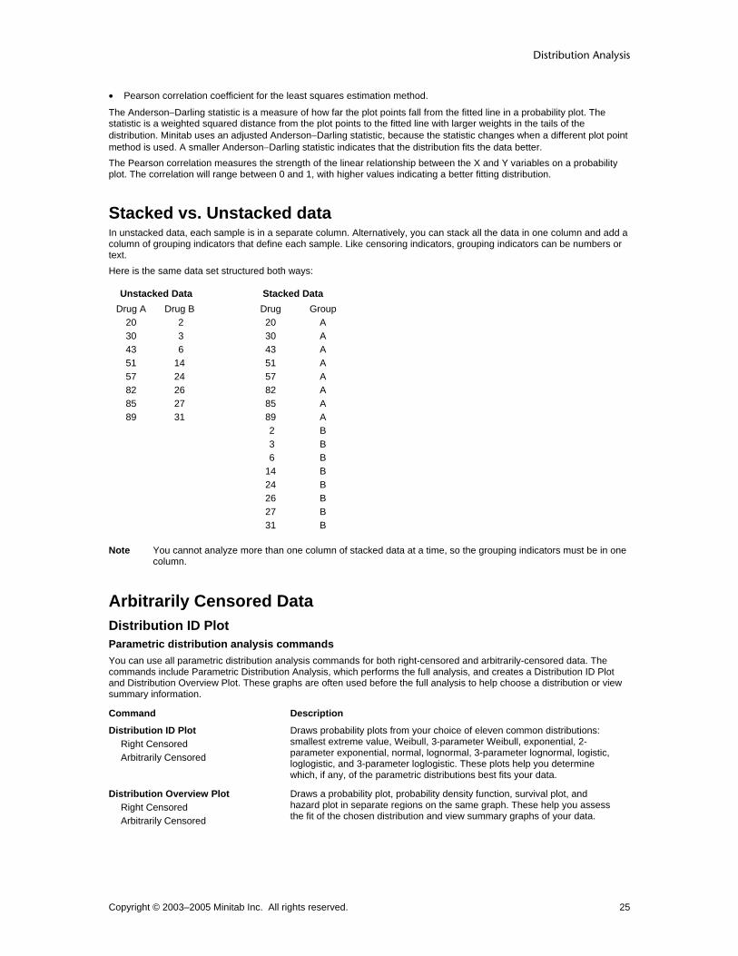
Stacked vs. Unstacked data In unstacked data, each sample is in a separate column. Alternatively, you can stack all the data in one column and add a column of grouping indicators that define each sample. Like censoring indicators, grouping indicators can be numbers or text. Here is the same data set structured both ways:
Unstacked Data Stacked Data Drug A
20 30 43 51 57 82 85 89
Drug B 2 3 6 14 24 26 27 31
Drug 20 30 43 51 57 82 85 89 2 3 6 14 24 26 27 31
Group A A A A A A A A B B B B B B B B
Note You cannot analyze more than one column of stacked data at a time, so the grouping indicators must be in one column.
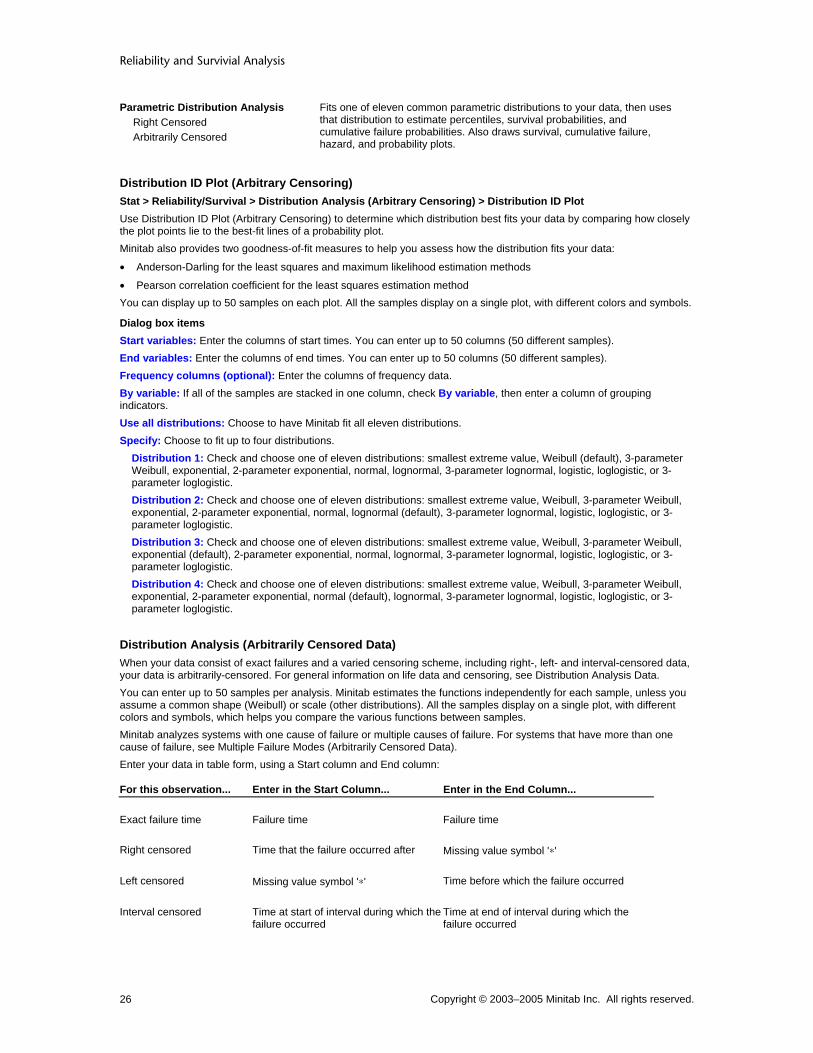
Arbitrarily Censored Data Distribution ID Plot Parametric distribution analysis commands You can use all parametric distribution analysis commands for both right-censored and arbitrarily-censored data. The commands include Parametric Distribution Analysis, which performs the full analysis, and creates a Distribution ID Plot and Distribution Overview Plot. These graphs are often used before the full analysis to help choose a distribution or view summary information.
Command Description
Distribution ID Plot Right Censored Arbitrarily Censored
Draws probability plots from your choice of eleven common distributions: smallest extreme value, Weibull, 3-parameter Weibull, exponential, 2-parameter exponential, normal, lognormal, 3-parameter lognormal, logistic, loglogistic, and 3-parameter loglogistic. These plots help you determine which, if any, of the parametric distributions best fits your data.
Distribution Overview Plot Right Censored Arbitrarily Censored
Draws a probability plot, probability density function, survival plot, and hazard plot in separate regions on the same graph. These help you assess the fit of the chosen distribution and view summary graphs of your data.
Reliability and Survivial Analysis
Copyright © 2003–2005 Minitab Inc. All rights reserved. 26
Parametric Distribution Analysis Right Censored Arbitrarily Censored
Fits one of eleven common parametric distributions to your data, then uses that distribution to estimate percentiles, survival probabilities, and cumulative failure probabilities. Also draws survival, cumulative failure, hazard, and probability plots.
Distribution ID Plot (Arbitrary Censoring) Stat > Reliability/Survival > Distribution Analysis (Arbitrary Censoring) > Distribution ID Plot Use Distribution ID Plot (Arbitrary Censoring) to determine which distribution best fits your data by comparing how closely the plot points lie to the best-fit lines of a probability plot. Minitab also provides two goodness-of-fit measures to help you assess how the distribution fits your data:
• Anderson-Darling for the least squares and maximum likelihood estimation methods
• Pearson correlation coefficient for the least squares estimation method You can display up to 50 samples on each plot. All the samples display on a single plot, with different colors and symbols.
Dialog box items Start variables: Enter the columns of start times. You can enter up to 50 columns (50 different samples). End variables: Enter the columns of end times. You can enter up to 50 columns (50 different samples). Frequency columns (optional): Enter the columns of frequency data. By variable: If all of the samples are stacked in one column, check By variable, then enter a column of grouping indicators. Use all distributions: Choose to have Minitab fit all eleven distributions. Specify: Choose to fit up to four distributions.
Distribution 1: Check and choose one of eleven distributions: smallest extreme value, Weibull (default), 3-parameter Weibull, exponential, 2-parameter exponential, normal, lognormal, 3-parameter lognormal, logistic, loglogistic, or 3-parameter loglogistic. Distribution 2: Check and choose one of eleven distributions: smallest extreme value, Weibull, 3-parameter Weibull, exponential, 2-parameter exponential, normal, lognormal (default), 3-parameter lognormal, logistic, loglogistic, or 3-parameter loglogistic. Distribution 3: Check and choose one of eleven distributions: smallest extreme value, Weibull, 3-parameter Weibull, exponential (default), 2-parameter exponential, normal, lognormal, 3-parameter lognormal, logistic, loglogistic, or 3-parameter loglogistic. Distribution 4: Check and choose one of eleven distributions: smallest extreme value, Weibull, 3-parameter Weibull, exponential, 2-parameter exponential, normal (default), lognormal, 3-parameter lognormal, logistic, loglogistic, or 3-parameter loglogistic.
Distribution Analysis (Arbitrarily Censored Data) When your data consist of exact failures and a varied censoring scheme, including right-, left- and interval-censored data, your data is arbitrarily-censored. For general information on life data and censoring, see Distribution Analysis Data. You can enter up to 50 samples per analysis. Minitab estimates the functions independently for each sample, unless you assume a common shape (Weibull) or scale (other distributions). All the samples display on a single plot, with different colors and symbols, which helps you compare the various functions between samples. Minitab analyzes systems with one cause of failure or multiple causes of failure. For systems that have more than one cause of failure, see Multiple Failure Modes (Arbitrarily Censored Data). Enter your data in table form, using a Start column and End column:
For this observation... Enter in the Start Column... Enter in the End Column...
Exact failure time Failure time Failure time
Right censored Time that the failure occurred after Missing value symbol '∗'
Left censored Missing value symbol '∗' Time before which the failure occurred
Interval censored Time at start of interval during which the failure occurred
Time at end of interval during which the failure occurred

Distribution Analysis
Copyright © 2003–2005 Minitab Inc. All rights reserved. 27
This data set illustrates tabled data. For observations with corresponding columns of frequency, see Using frequency columns.
Start End
* 10000 Left censored at 10000 hours.
10000 20000
20000 30000
30000 30000 Exact failures at 30000 hours.
30000 40000
40000 50000
50000 50000
50000 60000 Interval censored between 50000 and 60000 hours.
60000 70000
70000 80000
80000 90000
90000 * Right censored at 90000 hours.
When you have more than one sample, you can use separate columns for each sample. Alternatively, you can stack all the samples in one column, then set up a column of grouping indicators, which can be numbers or text. For an illustration, see Stacked vs. Unstacked data.
To make a distribution ID plot (arbitrarily censored data) 1 Choose Stat > Reliability/Survival > Distribution Analysis (Arbitrary Censoring) > Distribution ID Plot. 2 In Start variables, enter up to 50 columns of start times. 3 In End variables, enter up to 50 column of end times. The first start column is paired with the first end column, the
second start column is paired with the second end column, and so on. 4 If you have frequency columns, enter them in Frequency columns. 5 If all of the samples are stacked in one column, check By variable, and enter a column of grouping indicators in the
box. 6 Do one of the following:
• Choose Use all distributions to create probability plots for all eleven distributions. • Choose Specify to create up to four probability plots with the distributions of your choice.
7 If you like, use any of the dialog box options, then click OK.
Distribution ID Plot (Arbitrary Censoring) − Options Stat > Reliability/Survival > Distribution Analysis (Arbitrary Censoring) > Distribution ID Plot > Options You can choose the method used to estimate the parameters. You can also estimate percentiles for specified percents, specify the x-axis minimum and maximum, and add your own title.
Dialog box items Estimation Method
Least Squares (failure time(X) on rank(Y)): Choose to estimate the distribution parameters using the least squares (XY) method, which are estimated by fitting a regression line to the points in a probability plot. Maximum Likelihood: Choose to estimate the distribution parameters using the maximum likelihood method, which are estimated by maximizing the likelihood function.
Estimate percentiles for these percents: Enter the additional percents for which you want to estimate percentiles. You can enter individual percents (0 < P < 100) or a column of percents. Show graphs of different variables or by levels: Choose to display the graphs overlaid on the same graph or on separate graphs.
Use default values: Choose to use the default values for the minimum and maximum X scale. Use: Choose to enter your own values for the X scale minimum and maximum.
Minimum X scale: Enter a value for the minimum X scale.

Reliability and Survivial Analysis
Copyright © 2003–2005 Minitab Inc. All rights reserved. 28
Maximum X scale: Enter a value for the maximum X scale. Title: To replace the default title with your own title, type the desired text in this box.
Example of a Distribution ID Plot for arbitrarily-censored data Suppose you work for a company that manufactures tires. You are interested in finding out how many miles it takes for various proportions of the tires to "fail," or wear down to 2/32 of an inch of tread. You are especially interested in knowing how many of the tires last past 45,000 miles. You plan to get this information by using Parametric Distribution Analysis (Arbitrary Censoring), which requires you to specify the distribution for your data. Distribution ID Plot − Arbitrary Censoring can help you choose that distribution. You inspect each good tire at regular intervals (every 10,000 miles) to see if the tire has failed, then enter the data into the Minitab worksheet. 1 Open the worksheet TIREWEAR.MTW. 2 Choose Stat > Reliability/Survival > Distribution Analysis (Arbitrary Censoring) > Distribution ID Plot. 3 In Start variables, enter Start. In End variables, enter End. 4 In Frequency columns, enter Freq. 5 Choose Specify. Leave the first three distributions at the default. From Distribution 4, choose Smallest extreme
value. Click OK.
Session window output
Distribution ID Plot: Start = Start and End = End Using frequencies in Freq Goodness-of-Fit Anderson-Darling Correlation Distribution (adj) Coefficient Weibull 2.387 0.948 Lognormal 2.960 0.880 Exponential 6.411 * Smallest Extreme Value 2.325 0.998 Table of Percentiles Standard 95% Normal CI Distribution Percent Percentile Error Lower Upper Weibull 1 15065.1 4005.60 8946.43 25368.5 Lognormal 1 19317.3 1249.06 17018.0 21927.3 Exponential 1 497.954 15.2114 469.015 528.678 Smallest Extreme Value 1 9380.16 2509.70 4461.24 14299.1 Weibull 5 27623.1 4395.50 20222.1 37732.9 Lognormal 5 27495.1 1333.82 25001.3 30237.6 Exponential 5 2541.38 77.6336 2393.68 2698.18 Smallest Extreme Value 5 33699.7 1700.67 30366.5 37033.0 Weibull 10 36103.8 4050.07 28977.9 44982.1 Lognormal 10 33188.2 1335.70 30670.8 35912.1 Exponential 10 5220.19 159.466 4916.81 5542.28 Smallest Extreme Value 10 44439.8 1356.88 41780.4 47099.3 Weibull 50 72756.0 1504.02 69867.1 75764.4 Lognormal 50 64458.5 1238.08 62077.0 66931.3 Exponential 50 34342.6 1049.09 32346.8 36461.6 Smallest Extreme Value 50 72547.7 635.757 71301.6 73793.8
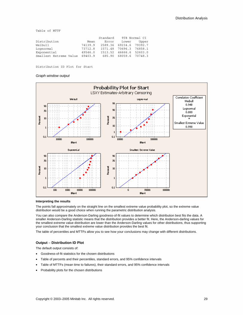
Distribution Analysis
Copyright © 2003–2005 Minitab Inc. All rights reserved. 29
Table of MTTF Standard 95% Normal CI Distribution Mean Error Lower Upper Weibull 74139.9 2589.36 69234.6 79392.7 Lognormal 73712.8 1571.48 70696.3 76858.1 Exponential 49546.0 1513.52 46666.6 52603.0 Smallest Extreme Value 69403.9 685.90 68059.6 70748.3 Distribution ID Plot for Start
Graph window output
Interpreting the results The points fall approximately on the straight line on the smallest extreme value probability plot, so the extreme value distribution would be a good choice when running the parametric distribution analysis. You can also compare the Anderson-Darling goodness-of-fit values to determine which distribution best fits the data. A smaller Anderson-Darling statistic means that the distribution provides a better fit. Here, the Anderson-darling values for the smallest extreme value distribution are lower than the Anderson-Darling values for other distributions, thus supporting your conclusion that the smallest extreme value distribution provides the best fit. The table of percentiles and MTTFs allow you to see how your conclusions may change with different distributions.
Output − Distribution ID Plot The default output consists of:
• Goodness-of-fit statistics for the chosen distributions
• Table of percents and their percentiles, standard errors, and 95% confidence intervals
• Table of MTTFs (mean time to failures), their standard errors, and 95% confidence intervals
• Probability plots for the chosen distributions

Reliability and Survivial Analysis
Copyright © 2003–2005 Minitab Inc. All rights reserved. 30
For example,
Distribution ID Plot: Temp80 Goodness-of-Fit Anderson-Darling Correlation Distribution (adj) Coefficient Weibull 67.606 0.986 Lognormal 67.656 0.982 Exponential 71.519 * Normal 67.589 0.987 Table of Percentiles Standard 95% Normal CI Distribution Percent Percentile Error Lower UpperWeibull 1 17.7339 2.44778 13.5305 23.2431Lognormal 1 21.5948 2.46626 17.2638 27.0123Exponential 1 0.737540 0.115720 0.542291 1.00309Normal 1 15.1273 4.41131 6.48126 23.7733 Weibull 5 27.7571 2.85714 22.6859 33.9618Lognormal 5 28.6233 2.61498 23.9307 34.2361Exponential 5 3.76414 0.590591 2.76766 5.11939Normal 5 27.3722 3.71588 20.0893 34.6552 Weibull 10 33.8299 2.97051 28.4812 40.1830Lognormal 10 33.2625 2.68093 28.4020 38.9548Exponential 10 7.73184 1.21312 5.68499 10.5156Normal 10 33.9000 3.38602 27.2635 40.5365 Weibull 50 56.7777 2.90747 51.3558 62.7720Lognormal 50 56.5033 3.38997 50.2348 63.5539Exponential 50 50.8663 7.98090 37.4005 69.1804Normal 50 56.9267 2.63143 51.7692 62.0842 Table of MTTF Standard 95% Normal CI Distribution Mean Error Lower Upper Weibull 56.6179 2.7394 51.4955 62.2497 Lognormal 61.5452 3.8295 54.4791 69.5279 Exponential 73.3846 11.5140 53.9575 99.8063 Normal 56.9267 2.6314 51.7692 62.0842 Distribution ID Plot for Temp80
Overview Plot Parametric distribution analysis commands You can use all parametric distribution analysis commands for both right-censored and arbitrarily-censored data. The commands include Parametric Distribution Analysis, which performs the full analysis, and creates a Distribution ID Plot and Distribution Overview Plot. These graphs are often used before the full analysis to help choose a distribution or view summary information.
Command Description
Distribution ID Plot Right Censored Arbitrarily Censored
Draws probability plots from your choice of eleven common distributions: smallest extreme value, Weibull, 3-parameter Weibull, exponential, 2-parameter exponential, normal, lognormal, 3-parameter lognormal, logistic, loglogistic, and 3-parameter loglogistic. These plots help you determine which, if any, of the parametric distributions best fits your data.

Distribution Analysis
Copyright © 2003–2005 Minitab Inc. All rights reserved. 31
Distribution Overview Plot Right Censored Arbitrarily Censored
Draws a probability plot, probability density function, survival plot, and hazard plot in separate regions on the same graph. These help you assess the fit of the chosen distribution and view summary graphs of your data.
Parametric Distribution Analysis Right Censored Arbitrarily Censored
Fits one of eleven common parametric distributions to your data, then uses that distribution to estimate percentiles, survival probabilities, and cumulative failure probabilities. Also draws survival, cumulative failure, hazard, and probability plots.
Distribution Overview Plot (Arbitrary Censoring) Stat > Reliability/Survival > Distribution Analysis (Arbitrary Censoring) > Distribution Overview Plot Use Distribution Overview Plot to generate a layout of plots that allow you to view your life data in different ways on one graph. You can draw a parametric overview plot by selecting a distribution for your data, or a nonparametric overview plot. The parametric display includes a probability plot (for a selected distribution), a survival (or reliability) plot, a probability density function, and a hazard plot. The nonparametric display depends on the type of data: if you have right-censored data Minitab displays a Kaplan-Meier survival plot and a hazard plot or an Actuarial survival plot and hazard plot, and if you have arbitrarily-censored data, Minitab displays a Turnbull survival plot or an Actuarial survival plot and hazard plot. These functions are all typical ways of describing the distribution of failure time data. You can enter up to fifty samples per analysis. Minitab estimates the functions independently for each sample. All of the samples display on a single plot, in different colors and symbols, which helps you compare their various functions. To draw these plots with more information, see one of the Distribution Analysis Commands.
Dialog box items Start variables: Enter the columns of start times. You can enter up to 50 columns (50 different samples). End variables: Enter the columns of end times. You can enter up to 50 columns (50 different samples). Frequency columns (optional): Enter the columns of frequency data. By variable: If all of the samples are stacked in one column, check By variable, and enter a column of grouping indicators in the box. Parametric analysis: Choose to perform a parametric distribution analysis.
Distribution: Choose one of eleven distributions: smallest extreme value, Weibull (default), 3-parameter Weibull, exponential, 2-parameter exponential, normal, lognormal, 3-parameter lognormal, logistic, loglogistic, or 3-parameter loglogistic.
Nonparametric analysis: Choose to perform a nonparametric distribution analysis.
Distribution Analysis (Arbitrarily Censored Data) When your data consist of exact failures and a varied censoring scheme, including right-, left- and interval-censored data, your data is arbitrarily-censored. For general information on life data and censoring, see Distribution Analysis Data. You can enter up to 50 samples per analysis. Minitab estimates the functions independently for each sample, unless you assume a common shape (Weibull) or scale (other distributions). All the samples display on a single plot, with different colors and symbols, which helps you compare the various functions between samples. Minitab analyzes systems with one cause of failure or multiple causes of failure. For systems that have more than one cause of failure, see Multiple Failure Modes (Arbitrarily Censored Data). Enter your data in table form, using a Start column and End column:
For this observation... Enter in the Start Column... Enter in the End Column...
Exact failure time Failure time Failure time
Right censored Time that the failure occurred after Missing value symbol '∗'
Left censored Missing value symbol '∗' Time before which the failure occurred
Interval censored Time at start of interval during which the failure occurred
Time at end of interval during which the failure occurred

Reliability and Survivial Analysis
Copyright © 2003–2005 Minitab Inc. All rights reserved. 32
This data set illustrates tabled data. For observations with corresponding columns of frequency, see Using frequency columns.
Start End
* 10000 Left censored at 10000 hours.
10000 20000
20000 30000
30000 30000 Exact failures at 30000 hours.
30000 40000
40000 50000
50000 50000
50000 60000 Interval censored between 50000 and 60000 hours.
60000 70000
70000 80000
80000 90000
90000 * Right censored at 90000 hours.
When you have more than one sample, you can use separate columns for each sample. Alternatively, you can stack all the samples in one column, then set up a column of grouping indicators, which can be numbers or text. For an illustration, see Stacked vs. Unstacked data.
To make a distribution overview plot (arbitrarily-censored data) 1 Choose Stat > Reliability/Survival > Distribution Analysis (Arbitrary Censoring) > Distribution Overview Plot. 2 In Start variables, enter up to 50 columns of start times. 3 In End variables, enter up to 50 columns of end times. 4 If you have frequency columns, enter the columns in Frequency columns. 5 If all of the samples are stacked in one column, check By variable, and enter a column of grouping indicators in the
box. 6 Choose to draw a parametric or nonparametric plot:
• Parametric plot− Choose Parametric analysis. From Distribution, choose to plot one of eleven distributions. • Nonparametric plot− Choose Nonparametric analysis.
7 If you like, use any of the dialog box items, then click OK.
Distribution Overview Plot (Arbitrary Censoring) − Options Stat > Reliability/Survival > Distribution Analysis (Arbitrary Censoring) > Distribution Overview Plot > Options You can choose the method used to estimate the parameters. You can also specify the x-axis minimum and maximum, and add your own title.
Dialog box items Estimation Method
Least Squares (failure time(X) on rank(Y)): Choose to estimate the distribution parameters using the least squares (XY) method, which are estimated by fitting a regression line to the points in a probability plot. Maximum Likelihood: Choose to estimate the distribution parameters using the maximum likelihood method, which are estimated by maximizing the likelihood function.
Show graphs of different variables or by levels Choose to display the graphs overlaid on the same graph or on separate graphs. Minimum and Maximum X Scale:
Use default values: Choose to use the default values for the minimum and maximum X scale. Use: Choose to enter your own values for the X scale minimum and maximum.
Minimum X scale: Enter a value for the minimum X scale. Maximum X scale: Enter a value for the maximum X scale.
Title: To replace the default title with your own title, type the desired text in this box.

Distribution Analysis
Copyright © 2003–2005 Minitab Inc. All rights reserved. 33
Example of a Distribution Overview Plot with arbitrarily-censored data Suppose you work for a company that manufactures tires. You are interested in finding out how many miles it takes for various proportions of the tires to "fail," or wear down to 2/32 of an inch of tread. You are especially interested in knowing how many of the tires last past 45,000 miles. You plan to get this information by using Parametric Distribution Analysis (Arbitrary Censoring), but first you want to have a quick look at your data from different perspectives. You inspect each good tire at regular intervals (every 10,000 miles) to see if the tire has failed, then enter the data into the Minitab worksheet. 1 Open the worksheet TIREWEAR.MTW.
2 Choose Stat > Reliability/Survival > Distribution Analysis (Arbitrary Censoring) > Distribution Overview Plot. 3 In Start variables, enter Start. In End variables, enter End. 4 In Frequency columns, enter Freq. 5 In Distribution, choose Smallest extreme value. Click OK.
Session window output
Distribution Overview Plot: Start = Start and End = End Using frequencies in Freq Goodness-of-Fit Anderson-Darling CorrelationDistribution (adj) CoefficientSmallest Extreme Value 2.325 0.998 Distribution Overview Plot for Start
Graph window output

Reliability and Survivial Analysis
Copyright © 2003–2005 Minitab Inc. All rights reserved. 34
Interpreting the results These four plots describe the failure rate for tires over time. With these plots, you can determine that approximately 90% of the tires last past 45,000 miles.
Output − Distribution Overview Plot The distribution overview plot display differs depending on whether you select the parametric or nonparametric display. When you select a parametric display, you get:
• Goodness-of-fit statistics for the chosen distribution
• Probability plot, which displays estimates of the cumulative distribution function F(y) vs. failure time.
• Parametric survival (or reliability) plot, which displays the survival (or reliability) function 1-F(y) vs. failure time.
• Probability density function, which displays the curve that describes the distribution of your data, or f(y).
• Parametric hazard plot, which displays the hazard function or instantaneous failure rate, f(y)/(1-F(y)) vs. failure time. When you select a nonparametric display, you get:
• For right-censored data with Kaplan-Meier method - Kaplan-Meier survival plot - Nonparametric hazard plot based on the empirical hazard function
• For right-censored data with Actuarial method - Actuarial survival plot - Nonparametric hazard plot based on the empirical hazard function
• For arbitrarily-censored data with Turnbull method - Turnbull survival plot
• For arbitrarily-censored data with Actuarial method - Actuarial survival plot - Nonparametric hazard plot based on the empirical hazard function
The Kaplan-Meier survival estimates, Turnbull survival estimates, and empirical hazard function change values only at exact failure times, so the nonparametric survival and hazard curves are step functions. Parametric survival and hazard estimates are based on a fitted distribution and the curve will therefore be smooth. For example,
Distribution Overview Plot: Temp80 Goodness-of-Fit Anderson-Darling CorrelationDistribution (adj) CoefficientWeibull 67.606 0.986 Distribution Overview Plot for Temp80
Parametric Distribution Analysis Parametric distribution analysis commands You can use all parametric distribution analysis commands for both right-censored and arbitrarily-censored data. The commands include Parametric Distribution Analysis, which performs the full analysis, and creates a Distribution ID Plot and Distribution Overview Plot. These graphs are often used before the full analysis to help choose a distribution or view summary information.
Command Description
Distribution ID Plot Right Censored Arbitrarily Censored
Draws probability plots from your choice of eleven common distributions: smallest extreme value, Weibull, 3-parameter Weibull, exponential, 2-parameter exponential, normal, lognormal, 3-parameter lognormal, logistic, loglogistic, and 3-parameter loglogistic. These plots help you determine which, if any, of the parametric distributions best fits your data.

Distribution Analysis
Copyright © 2003–2005 Minitab Inc. All rights reserved. 35
Distribution Overview Plot Right Censored Arbitrarily Censored
Draws a probability plot, probability density function, survival plot, and hazard plot in separate regions on the same graph. These help you assess the fit of the chosen distribution and view summary graphs of your data.
Parametric Distribution Analysis Right Censored Arbitrarily Censored
Fits one of eleven common parametric distributions to your data, then uses that distribution to estimate percentiles, survival probabilities, and cumulative failure probabilities. Also draws survival, cumulative failure, hazard, and probability plots.
Parametric Distribution Analysis (Arbitrary Censoring) Stat > Reliability/Survival > Distribution Analysis (Arbitrary Censoring) > Parametric Distribution Analysis Use Parametric Distribution Analysis-Arbitrary Censoring when you have data that is arbitrarily censored or actual failure times. You can fit one of eleven common distributions to your data, estimate percentiles, survival probabilities, and cumulative failure probabilities, evaluate the appropriateness of the distribution, and draw survival, cumulative failure, hazard, and probability plots. Use the probability plot to see if the distribution fits your data. To compare the fits of different distributions, see Distribution ID Plot (Arbitrary Censoring), which draws four probability plots in separate regions on the same graph. If no parametric distribution fits your data, use one of the nonparametric distribution analysis commands. To view your data in different ways, see Distribution Overview Plot (Arbitrary Censoring).
Dialog box items Start variables: Enter the columns of start times. You can enter up to 50 columns (50 different samples). End variables: Enter the columns of end times. You can enter up to 50 columns (50 different samples). Frequency columns (optional): Enter the columns of frequency data. By variable: If all of the samples are stacked in one column, check By variable, and enter a column of grouping indicators in the box Assumed distribution: Choose one of eleven common distributions: smallest extreme value, Weibull (default), 3-parameter Weibull, exponential, 2-parameter exponential, normal, lognormal 3-parameter lognormal, logistic, loglogistic, and 3 parameter loglogistic distributions.
Distribution Analysis (Arbitrarily Censored Data) When your data consist of exact failures and a varied censoring scheme, including right-, left- and interval-censored data, your data is arbitrarily-censored. For general information on life data and censoring, see Distribution Analysis Data. You can enter up to 50 samples per analysis. Minitab estimates the functions independently for each sample, unless you assume a common shape (Weibull) or scale (other distributions). All the samples display on a single plot, with different colors and symbols, which helps you compare the various functions between samples. Minitab analyzes systems with one cause of failure or multiple causes of failure. For systems that have more than one cause of failure, see Multiple Failure Modes (Arbitrarily Censored Data). Enter your data in table form, using a Start column and End column:
For this observation... Enter in the Start Column... Enter in the End Column...
Exact failure time Failure time Failure time
Right censored Time that the failure occurred after Missing value symbol '∗'
Left censored Missing value symbol '∗' Time before which the failure occurred
Interval censored Time at start of interval during which the failure occurred
Time at end of interval during which the failure occurred
This data set illustrates tabled data. For observations with corresponding columns of frequency, see Using frequency columns.

Reliability and Survivial Analysis
Copyright © 2003–2005 Minitab Inc. All rights reserved. 36
Start End
* 10000 Left censored at 10000 hours.
10000 20000
20000 30000
30000 30000 Exact failures at 30000 hours.
30000 40000
40000 50000
50000 50000
50000 60000 Interval censored between 50000 and 60000 hours.
60000 70000
70000 80000
80000 90000
90000 * Right censored at 90000 hours.
When you have more than one sample, you can use separate columns for each sample. Alternatively, you can stack all the samples in one column, then set up a column of grouping indicators, which can be numbers or text. For an illustration, see Stacked vs. Unstacked data.
To do a parametric distribution analysis (arbitrarily censored data) 1 Choose Stat > Reliability/Survival > Distribution Analysis (Arbitrary Censoring) > Parametric Distribution
Analysis. 2 In Start variables, enter up to 50 columns of start times. 3 In End variables, enter up to 50 columns of end times. 4 If you have frequency columns, enter them in Frequency columns. 5 If all of the samples are stacked in one column, check By variable, and enter a column of grouping indicators in the
box. 6 If you like, use any of the dialog box options, then click OK.
Choosing a Distribution with a Threshold Parameter The threshold parameter, γ , provides an estimate of the earliest time a failure may occur. The threshold parameter locates the distribution along the time scale and has the same units as time, such as hours, miles, or cycles.
• When γ = 0, the distribution starts at the origin.
• When γ > 0, the distribution starts to the right of the origin. The period from 0 to γ is the failure free operating period.
• When γ < 0, the distribution starts to the left of the origin. A negative γ indicates that failures have occurred prior to the beginning of a test.
Choose a distribution with a threshold parameter (3-parameter Weibull, 2-parameter exponential, 3-parameter lognormal, or 3-parameter loglogistic) when you want to estimate the earliest time-to-failure. The two probability plots show the same

Distribution Analysis
Copyright © 2003–2005 Minitab Inc. All rights reserved. 37
data fit to a Weibull and a 3-parameter Weibull distribution. The Weibull does not account for the threshold parameter and displays as a curve on probability paper. The 3-parameter Weibull adjusts for γ and the points appear straighter.
Note The threshold parameter is assumed fixed when calculating confidence intervals with the 3-parameter lognormal and 2-parameter exponential distributions.
Percentiles By what time do half of the engine windings fail? How long until 10% of the blenders stop working? You are looking for percentiles. The parametric distribution analysis commands automatically display a table of percentiles in the Session window. By default, Minitab displays the percentiles 1-10, 20, 30, 40, 50, 60, 70, 80, and 90-99. In this example, we entered failure times (in months) for engine windings.
Table of Percentiles Standard 95.0% Normal CIPercent Percentile Error Lower Upper 1 10.0765 2.78453 5.86263 17.3193 2 13.6193 3.23157 8.55426 21.6834 3 16.2590 3.48898 10.6767 24.7601 4 18.4489 3.66352 12.5009 27.2270
As shown in the first row of the table, at about 10 months (Percentile), 1% of the windings failed. The values in the Percentile column are estimates of the times at which the corresponding percent of the units failed. The table also includes standard errors and approximate 95.0% confidence intervals for each percentile. In the Estimate subdialog box, you can specify a different confidence level for all confidence intervals. You can also request percentiles to be added the default table.
Survival Probabilities − Parametric Distribution Analysis What is the probability of an engine winding running past a given time? How likely is it that a cancer patient will live five years after receiving a certain drug? You are looking for survival probabilities, which are estimates of the proportion of units that survive past a given time. When you request survival probabilities in the Estimate subdialog box, the parametric distribution analysis commands display them in the Session window. Here, for example, we requested a survival probability for engine windings running at 70 months:

Reliability and Survivial Analysis
Copyright © 2003–2005 Minitab Inc. All rights reserved. 38
Table of Survival Probabilities 95.0% Normal CI Time Probability Lower Upper 70.0000 0.4076 0.2894 0.5222
As shown in the table above, 40.76% of the engine windings last past 70 months.
Parametric Distribution Analysis − Failure Mode Stat > Reliability/Survival > Distribution Analysis (Right Censoring) or Distribution Analysis (Arbitrary Censoring) > Parametric Distribution Analysis > FMode Use to estimate the overall reliability of your system when multiple causes of failure exist in order to investigate the reliability of the individual failure modes. This option is available for both right-censored and arbitrarily censored data.
Dialog box items Use failure mode columns: Enter the columns containing the failure modes. To represent censored observations in the failure mode column, use an asterisk (*) for numeric columns or a space for text columns. Failure Mode Options
Use all failure modes: Choose to include all failure modes in the analysis. Use failure modes: Enter the failure modes to include in the analysis. Eliminate failure modes: Enter the failure modes to exclude from the analysis.
Create right censored observations using (Only available with arbitrary censoring.) Use to determine how Minitab will create right-censored observations for other failure modes when data are interval censored.
Midpoint of intervals: Choose if a failure for any one failure mode causes the experiment to end. Right endpoint of intervals: Choose if the experiment continues until the right endpoint when a failure in the interval occurs.
Change Distribution for Levels Use only if distribution is different from that selected in the main dialog box. Level: Enter failure mode, then choose the corresponding distribution for each failure mode.
Parametric Distribution Analysis − Estimate Stat > Reliability/Survival > Distribution Analysis (Right Censoring) or Distribution Analysis (Arbitrary Censoring) > Parametric Distribution Analysis > Estimate Choose the estimation used to estimate percentiles and survival probabilities for specified values. For more information on selecting estimation methods, see Least squares estimates versus maximum likelihood estimates. You can also enter a confidence level that Minitab will use for all confidence intervals.
Dialog box items Estimation Method
Least Squares (failure time(X) on rank(Y)): Choose to estimate the distribution parameters using the least squares (XY) method, which fits a regression line to the points in a probability plot. Maximum Likelihood: Choose to estimate the distribution parameters using the maximum likelihood method, which maximizes the likelihood function.
Assume common shape (slope−Weibull) or scale (1/slope−other dists): Check to estimate the parameters while assuming a common shape or scale parameter. Bayes analysis
Set shape (slope−Weibull) or scale (1/slope−other dists) at: Enter a value for the shape or scale parameter for all the response variables, or enter a list of values for the shape or scale that is equal in length to the number of variables. Set threshold at: Enter a value for the threshold parameter for all the variables, or enter a list of values equal to the number of response variables. Minitab estimates threshold parameters if you do not provide values to use.
Estimate percentiles for these additional percents: Enter the additional percents for which you want to estimate percentiles. You can enter individual percents (0 < P < 100) or a column of percents. Estimate probabilities for these times (values): Enter one or more times or a column of times for which you want to calculate survival probabilities or cumulative failure probabilities.
Estimate survival probabilities: Choose to estimate survival probabilities. Estimate cumulative failure probabilities: Choose to estimate cumulative failure probabilities.
Confidence level: Enter a confidence level for all of the confidence intervals. The default is 95.0%.

Distribution Analysis
Copyright © 2003–2005 Minitab Inc. All rights reserved. 39
Confidence intervals: Choose to use two-sided confidence intervals (the default) or just an upper or lower confidence interval.
To draw conclusions when you have few or no failures 1 In the main dialog box, click Estimate. 3 Under Estimation Method, choose Maximum Likelihood. 2 Depending on your distribution, under Bayes Analysis:
• In Set shape (slope−Weibull) or scale (1/slope−other dists) at, enter the shape or scale value. • In Set threshold at, enter the threshold value.
3 Click OK. For more information, see Drawing conclusions when you have few or no failures.
To choose the method for estimating parameters 1 In the main dialog box, click Estimate. 2 Under Estimation Method, choose Least Squares (the default) or Maximum Likelihood. 3 Click OK.
To request additional percentiles 1 In the main dialog box, click Estimate. 2 In Estimate percentiles for these additional percents, enter the additional percents for which you want to estimate
percentiles. You can enter individual percents (0 < P < 100) or a column of percents. 3 Click OK.
To request parametric survival probabilities 1 In the main dialog box, click Estimate. 2 In Estimate probabilities for these times (values), enter one or more times, or a column of times for which you want
to calculate survival probabilities. 3 Click OK.
To change confidence levels 1 In the main dialog box, click Estimate. 2 In Confidence level, enter a value. 3 Click OK.
Least squares estimates versus maximum likelihood estimates Least squares estimates are calculated by fitting a regression line to the points in a probability plot. The line is formed by regressing time to failure or log (time to failure) (X) on the transformed percent (Y). Maximum likelihood estimates are calculated by maximizing the likelihood function. The likelihood function describes, for each set of distribution parameters, the chance that the true distribution has the parameters based on the sample. Here are the major advantages of each method:
Least squares (LSXY) • Better graphical display to the probability plot because the line is fitted to the points on a probability plot.
• For small or heavily censored sample, LSXY is more accurate than MLE. MLE tends to overestimate the shape parameter for a Weibull distribution and underestimate the scale parameter in other distributions. Therefore, MLE will tend to overestimate the low percentiles.
Maximum likelihood (MLE) • Distribution parameter estimates are more precise than least squares (XY).
• MLE allows you to perform an analysis when there are no failures. When there is only one failure and some right-censored observations, the maximum likelihood parameter estimates may exist for a Weibull distribution.
• The maximum likelihood estimation method has attractive mathematical qualities.

Reliability and Survivial Analysis
Copyright © 2003–2005 Minitab Inc. All rights reserved. 40
When possible, both methods should be tried; if the results are consistent, then there is more support for your conclusions. Otherwise, you may want to use the more conservative estimates or consider the advantages of both approaches and make a choice for your problem.
Estimating the distribution parameters You can choose to estimate the parameters using either the least squares (XY) method or the maximum likelihood method (modified Newton-Raphson algorithm). Or, if you like, you can set your own parameters. In this case, no estimation is done; all results − such as the percentiles − are based on the parameters you enter. Least squares estimates are calculated by fitting a regression line to the points in a probability plot. The line is formed by regressing time to failure or log (time to failure) (X) on the transformed percent (Y). When Minitab estimates the parameters using the maximum likelihood method, you can:
• Enter starting values for the algorithm. The maximum likelihood solution may not converge if the starting estimates are not in the neighborhood of the true solution. You may want to enter reasonable starting values for parameter estimates: − For Weibull, enter shape and scale. − For exponential, enter mean. − For other 2-parameter distributions, enter location and scale. − For 2-parameter exponential, enter scale and threshold. − For 3-parameter Weibull, enter shape, scale, and threshold. − For other 3-parameter distributions, enter location, scale, and threshold.
• Change the maximum number of iterations for reaching convergence (the default is 20). Minitab obtains maximum likelihood estimates through an iterative process. If the maximum number of iterations is reached before convergence, the algorithm terminates.
When you set historical parameters, you can fix all parameter or you can estimate at least one parameter. Estimate at least one parameter by:
− Fixing the shape OR scale − Fixing the threshold − Fixing the shape OR scale AND threshold
Drawing conclusions when you have few or no failures When you have few or no failures, you can use historical values for distribution parameters to improve your analysis. Providing historical parameters makes the resulting analysis more precise, if your values are an appropriate choice. If your data come from a Weibull or exponential distribution, you can do a Bayes analysis to obtain lower confidence bounds for parameters, percentiles, survival probabilities, and cumulative failure probabilities. If you collect life data and have no failures, Minitab can still analyze when all of the following are met:
• The data come from a Weibull or exponential distribution.
• The data are right-censored.
• The maximum likelihood method will be used to estimate parameters.
• You provide a historical value for the shape parameter (Weibull). If your data are from an exponential distribution, Minitab automatically assigns a shape parameter of 1.
Note If your data come from a three−parameter Weibull or two−parameter exponential, you must also provide a historical value for the threshold parameter.
For example, your reliability specifications require that the 5th percentile is at least 12 months. You run a Bayes analysis on data with no failures, and then examine the lower confidence bound to substantiate that the product is at least as good as specifications require. If the lower confidence bound for the 5th percentile is 13.1 months, you conclude that your product meets specifications and terminate the test. See Demonstration Test Plans to determine the optimal testing time or number of test units to use.
Parametric Distribution Analysis − Test Stat > Reliability/Survival > Distribution Analysis (Right Censoring) or Distribution Analysis (Arbitrary Censoring) > Parametric Distribution Analysis > Test Tests whether distribution parameters for a sample equal specified values, and whether two or more samples share the same shape, scale, location, or threshold parameters. Minitab performs Wald Tests [7] and provides Bonferroni 95.0% confidence intervals for the following hypothesis tests:
Distribution Analysis
Copyright © 2003–2005 Minitab Inc. All rights reserved. 41
• Whether the distribution parameters (scale, shape, location, or threshold) are consistent with specified values
• Whether the sample comes from the historical distribution
• Whether two or more samples come from the same population
• Whether two or more samples share the same shape, scale, location, or threshold parameters
Dialog box items Consistency of Sample with Value
Test shape (slope−Weibull) or scale (1/slope−other dists) equal to: Enter a test value to compare the sample's shape (Weibull) or scale (other distributions). Test scale (Weibull or expo) or location (other dists) equal to: Enter a test value to compare the sample's scale (Weibull or exponential) or location (other distributions). Test threshold equal to: Enter a test value to compare the sample's threshold.
Equality of Parameters
Test for equal shape (slope−Weibull) or scale (1/slope−other distributions): Check to test whether two or more samples have the same shape or scale. Test for equal scale (Weibull or expo) or location (other distributions): Check to test whether two or more samples have the same scale or location. Test for equal threshold: Check to test whether two or more samples have the same threshold.
Note For 2-parameter distributions, check the first two Equality of Parameters options to test whether two or more samples come from the same population. For 3-parameter distributions, check all Equality of Parameters options, to test the same.
To compare distribution parameters to a specified value 1 In the main dialog box, click Test. 2 Do one or more of the following:
• In Test shape (slope−Weibull) or scale (1/slope−other dists) equal to, enter the test value. • In Test scale (Weibull or expo) or location (other dists) equal to, enter the test value. • In Test threshold equal to, enter the test value.
3 Click OK.
To compare parameters from two or more distributions 1 In the main dialog box, click Test. 2 Do one or more of the following:
• Check Test for equal shape (slope−Weibull) or scale (1/slope−other distributions). • Check Test for equal scale (Weibull or expo) or location (other distributions). • Check Test for equal threshold.
3 Click OK.
To determine whether two or more samples come from the same population 1 In the main dialog box, click Test. 2 Do the following:
• Check Test for equal shape (slope−Weibull) or scale (1/slope−other dists). • Check Test for equal scale (Weibull or expo) or location (other distributions). • Check Test for equal threshold.
3 Click OK.
To test whether a sample comes from a historical distribution 1 In the main dialog box, click Test. 2 Do the following:
• In Test shape (slope−Weibull) or scale (1/slope−other dists) equal to, enter the parameter of a historical distribution.

Reliability and Survivial Analysis
Copyright © 2003–2005 Minitab Inc. All rights reserved. 42
• In Test scale (Weibull or expo) or location (other dists) equal to, enter the parameter of a historical distribution.
• In Test threshold equal to, enter the parameter of a historical distribution. 3 Click OK.
Parametric Distribution Analysis (Arbitrary Censoring) − Graphs Stat > Reliability/Survival > Distribution Analysis (Arbitrary Censoring) > Parametric Distribution Analysis > Graphs You can draw a probability plot, a survival plot, cumulative failure plot, and a hazard plot.
Dialog box items Probability plot: Check to display a probability plot. Survival plot: Check to display a survival plot. Cumulative failure plot: Check to display a cumulative failure plot. Display confidence intervals on above plots: Check to display confidence intervals on the probability, survival, and cumulative failure plots. Hazard plot: Check to display a hazard plot. Show graphs of different variables or by levels: Choose to display the graphs overlaid on the same graph or on separate graphs. Minimum X scale: Enter a minimum value to be contained within your scale. Maximum X scale: Enter a maximum value to be contained within your scale. X axis label: Enter text to identify your x-axis.
To draw a parametric survival plot 1 In the main dialog box, click Graphs. 2 Check Survival plot. 3 If you like, do any of the following:
• Uncheck Display confidence intervals on above plots to turn off the 95.0% confidence interval. (See To change confidence levels if you want to change from 95% confidence intervals.)
• In Minimum X scale and Maximum X scale, type values for the x-axis scale. • In X axis label, enter a label for the x-axis.
4 Click OK.
To modify the default probability plot 1 In the main dialog box, click Graphs. 2 Do any of the following:
To... Do... Specify the method used to obtain the plot points
See Tools > Options > Individual Graphs > Probability Plots to choose Median Rank (Benard), Mean Rank (Herd−Johnson), modified Kaplan−Meier (Hazen), or Kaplan−Meier method.
Choose what to plot when you have tied failure times
For Parametric Distribution Analysis (Right Censoring) Under Handle tied failure times by plotting, choose All points (default), Maximum of the tied points, or Average (median) of tied points.
Turn off the 95.0% confidence interval
Uncheck Display confidence intervals on above plots.
Choose how plots are displayed
Choose Overlaid on the same graph to have multiple samples plotted on the same graph, In separate panels on the same graph to have multiple samples plotted in separate panels all on the same graph, or On separate graphs to have each plot displayed separately.
Specify a minimum and/or maximum value for the x-axis scale
In Minimum X scale or Maximum X scale, enter values for the scale minimum and maximum.
Enter a label for the x-axis In X axis label, type a label.

Distribution Analysis
Copyright © 2003–2005 Minitab Inc. All rights reserved. 43
3 Click OK. 4 To change the confidence level for the 95.0% confidence interval to some other level, click Estimate. In Confidence
level, enter a value. Click OK. 5 To change the method used to obtain the fitted line, click Estimate. In Estimation Method, choose Least Squares
(default) or Maximum Likelihood. Click OK.
Cumulative failure plots Cumulative failure plots display the cumulative failure probabilities versus time. Each plot point represents the cumulative percentage of units failing at time t. The cumulative failure curve is surrounded by two outer lines − the approximate 95.0% confidence interval for the curve, which provide reasonable values for the "true" cumulative failure function.
Hazard plots − parametric distribution analysis The hazard plot displays the instantaneous failure rate for each time t. Often, the hazard rate is high at the beginning of the plot, low in the middle of the plot, then high again at the end of the plot. Thus, the curve often resembles the shape of a bathtub. The early period with high failure rate is often called the infant mortality stage. The middle section of the curve, where the failure rate is low, is the normal life stage. The end of the curve, where failure rate increases again, is the wearout stage. This particular example does not have the bathtub shape.

Reliability and Survivial Analysis
Copyright © 2003–2005 Minitab Inc. All rights reserved. 44
To draw a parametric hazard plot, check Hazard plot in the Graphs subdialog box.
Probability plots Use a probability plot to assess whether a particular distribution fits your data. The plot consists of:
• Plot points, which represent the proportion of failures up to a certain time. Minitab calculates the plot points using a nonparametric method. The observed failure times are plotted on the x-axis vs. the estimated cumulative probabilities (p) on the y-axis. Transformations of both the x and y data are needed to ensure that the plotted y values are a linear function of the plotted x values if the data are sampled from the particular distribution.
• Fitted line, which is a graphical representation of the percentiles. To make the fitted line, Minitab first calculates the percentiles for the various percents, based on the chosen distribution. The associated probabilities are then transformed and used as the y-variables. The percentiles may be transformed, depending on the distribution, and are used as the x-variables. The transformed scales, chosen to linearize the fitted line, differ depending on the distribution used.
• Confidence intervals, set of approximate 95.0% confidence intervals for the fitted line. For more information on probability plot calculations, see Methods and formulas - parametric distribution analysis. Because the plot points do not depend on any distribution, they would be the same (before being transformed) for any probability plot made. The fitted line, however, differs depending on the parametric distribution chosen. So you can use the probability plot to assess whether a particular distribution fits your data. In general, the closer the points fall to the fitted line, the better the fit. Minitab provides two goodness of fit measures to help assess how the distribution fits your data. To choose from various methods to estimate the plot points, see Tools > Options > Individual Graphs > Probability Plots. To choose from various methods to obtain the fitted line, see Parametric Distribution Analysis − Estimate.
Tip To quickly compare the fit of up to eleven different distributions at once, see Distribution ID Plot (Right Censoring) or Distribution ID Plot (Arbitrary Censoring).
The Weibull probability plot below shows failure times associated with running engine windings at a temperature of 80° C:

Distribution Analysis
Copyright © 2003–2005 Minitab Inc. All rights reserved. 45
Survival plots Survival (or reliability) plots display the survival probabilities versus time. Each plot point represents the proportion of units surviving at time t. The survival curve is surrounded by two outer lines − the approximate 95.0% confidence interval for the curve, which provide reasonable values for the "true" survival function.

Reliability and Survivial Analysis
Copyright © 2003–2005 Minitab Inc. All rights reserved. 46
To draw a parametric survival plot 1 In the main dialog box, click Graphs. 2 Check Survival plot. 3 If you like, do any of the following:
• Uncheck Display confidence intervals on above plots to turn off the 95.0% confidence interval. (See To change confidence levels if you want to change from 95% confidence intervals.)
• In Minimum X scale and Maximum X scale, type values for the x-axis scale. • In X axis label, enter a label for the x-axis.
4 Click OK.
To modify the default probability plot 1 In the main dialog box, click Graphs. 2 Do any of the following:
To... Do... Specify the method used to obtain the plot points
See Tools > Options > Individual Graphs > Probability Plots to choose Median Rank (Benard), Mean Rank (Herd−Johnson), modified Kaplan−Meier (Hazen), or Kaplan−Meier method.
Choose what to plot when you have tied failure times
For Parametric Distribution Analysis (Right Censoring) Under Handle tied failure times by plotting, choose All points (default), Maximum of the tied points, or Average (median) of tied points.
Turn off the 95.0% confidence interval
Uncheck Display confidence intervals on above plots.
Choose how plots are displayed
Choose Overlaid on the same graph to have multiple samples plotted on the same graph, In separate panels on the same graph to have multiple samples plotted in separate panels all on the same graph, or On separate graphs to have each plot displayed separately.
Specify a minimum and/or maximum value for the x-axis scale
In Minimum X scale or Maximum X scale, enter values for the scale minimum and maximum.
Enter a label for the x-axis In X axis label, type a label.
3 Click OK. 4 To change the confidence level for the 95.0% confidence interval to some other level, click Estimate. In Confidence
level, enter a value. Click OK. 5 To change the method used to obtain the fitted line, click Estimate. In Estimation Method, choose Least Squares
(default) or Maximum Likelihood. Click OK.
Parametric Distribution Analysis − Results Stat > Reliability/Survival > Distribution Analysis (Right Censoring) or Distribution Analysis (Arbitrary Censoring) > Parametric Distribution Analysis > Results You can control the display of Session window output.
Dialog box items Control the Display of Results
Display nothing: Choose to suppress all Session window output. Variable information, censoring information, estimated parameters, log-likelihood, goodness-of-fit and tests of parameters: Choose to display censoring information and the estimation method. Minitab also displays the assumed distribution, parameter estimates, and tests of parameters. In addition, characteristics of distribution, table of percentiles and survival probabilities: Choose to also display the MTTF, standard deviation, median, quartile information, and percentiles. If you select survival probabilities in the Estimate subdialog box, Minitab also displays them.
Display analyses for individual failure modes according to display of results: Check to display the results chosen above for each failure mode. Show log-likelihood for each iteration of algorithm: Check to show the log-likelihood for each iteration of algorithm.

Distribution Analysis
Copyright © 2003–2005 Minitab Inc. All rights reserved. 47
Parametric Distribution Analysis − Options Stat > Reliability/Survival > Distribution Analysis (Right Censoring) or Distribution Analysis (Arbitrary Censoring) > Parametric Distribution Analysis > Options You can specify whether the distribution parameters should be calculated from the data or enter your own historical estimates.
Dialog box items Estimate parameters of distribution: Choose to estimate the distribution parameters from the data (the default).
Use starting estimates: Enter starting estimates for the parameters. Enter one column of values to be used for all samples, or several columns of values that match the order in which the corresponding variables appear in the Variables box in the main dialog box. Maximum number of iterations: Enter the maximum number of iterations. The default number of iterations is 20.
Use historical estimates: Enter one column of values to be used for all samples, or several columns of values which match the order in which the corresponding variables appear in the Variables box in the main dialog box.
To control estimation of the parameters 1 In the main dialog box, click Options. 2 If Least Squares is your estimation method, choose Use historical estimates.
If Maximum Likelihood is your estimation method, choose one of the following:
• Estimate parameters of distribution, to estimate the distribution parameters from the data.
• Use historical estimates, to enter your own estimates for the distribution parameters. 3 If you choose Estimate parameters of distribution, you can do any of the following:
− In Use starting estimates, enter columns of starting values based on your data structure. See Starting estimates for more information.
− In Maximum number of iterations, enter a positive integer to specify the maximum number of iterations for estimation.
4 If you choose Use historical estimates,
− Enter columns of historical values based on your data structure. See Historical estimates for more information.
5 Click OK.
Starting estimates and historical estimates You must enter starting estimates or historical estimates for each distribution of failures each parameter you wish to estimate. Each variable, By variable group level, and failure mode represents a unique distribution that requires estimates in one single column or in separate columns. See the following table for various scenarios: Variables with single failure modes:
Case Enter A single variable with a single failure mode. • Enter one column containing values for each parameter of your
distribution. Two or more variables, each with a single failure mode.
• Enter a single column containing values for each parameter for each variable.
• Enter one column of parameter estimates for each variable. A By variable with several group levels. • Enter a single column containing values for each parameter for
all group levels.
• Enter one column of values for each group level. If there are four group levels, enter four columns containing parameter estimates.

Reliability and Survivial Analysis
Copyright © 2003–2005 Minitab Inc. All rights reserved. 48
Variables with multiple failure modes:
Case Enter A single variable with a multiple failure modes.
• Enter a single column containing values for each parameter for each failure mode.
• Enter one column of parameter estimates for each failure mode. If there are three failure modes, enter three columns of parameter estimates.
Two or more variables, each with multiple failure modes.
• Enter a single column containing values for each parameter for each failure mode and variable.
• Enter one column of parameter estimates for each failure mode of each variable. If there are two variables with two failure modes, enter four columns of parameter estimates.
A By variable with several group levels and multiple failure modes.
• Enter a single column containing values for each parameter for each failure mode of each group level.
• Enter one column of parameter estimates for each failure mode of each group level. If there are two group levels with three failure modes each, enter six columns of parameter estimates.
Parameter estimates are assigned by failure mode then variable. Normally, the first column should contain the parameter estimates of failure mode 1, variable 1; the second column − parameter estimates of failure mode 1, variable 2, etc. If variable 2 does not have failure mode 1, the second column contains the parameter estimates of failure mode 2, variable 1.
Caution Do not enter starting estimates or historical estimates for failure modes that you have eliminated from the analysis.
Parametric Distribution Analysis − Storage Stat > Reliability/Survival > Distribution Analysis (Right Censoring) or Distribution Analysis (Arbitrary Censoring) > Parametric Distribution Analysis > Storage You can store characteristics of the fitted distribution and information on the distribution parameters in your worksheet. With multiple failure modes, you can store information pertaining to the overall distribution only.
Dialog box items Enter number of levels in by variable If all of the samples are stacked in one column, enter the number of levels the column of grouping indicators contains. Characteristics of Fitted Distribution
Percentiles: Check to store percentiles. Percents for percentiles: Check to store percents for percentiles. Standard error of percentiles: Check to store standard error of percentiles. Confidence limits for percentiles: Check to store confidence limits for percentiles. Times for probabilities: Check to store times for survival probabilities and cumulative failure probabilities. Available when you estimate survival probabilities or cumulative failure probabilities at different times. Survival probabilities: Check to store survival probabilities. Available when you estimate survival probabilities at different times. Confidence limits for survival probabilities: Check to store confidence limits for survival probabilities. Available when you estimate survival probabilities at different times. Cumulative failure probabilities: Check to store cumulative failure probabilities. Available when you estimate cumulative failure probabilities at different times. Confidence limits for cumulative failure probabilities: Check to store confidence limits for cumulative failure probabilities. Available when you estimate cumulative failure probabilities at different times.
Information on Parameters Choose to store the following when you have a single failure mode. Parameters estimates: Check to store parameter estimates. Standard error of estimates: Check to store standard error of parameter estimates. Confidence limits for parameters: Check to store confidence limits for parameters. Variance/covariance matrix: Check to store the variance / covariance matrix. Log-likelihood for last iteration: Check to store the log-likelihood ratio for the last iteration.

Distribution Analysis
Copyright © 2003–2005 Minitab Inc. All rights reserved. 49
Example of a parametric distribution analysis with arbitrarily censored data Suppose you work for a company that manufactures tires. You are interested in finding out how many miles it takes for various proportions of the tires to "fail," or wear down to 2/32 of an inch of tread. You are especially interested in knowing how many of the tires last past 45,000 miles. You inspect each tire at regular intervals (every 10,000 miles) to see if the tire has failed, then enter the data into the Minitab worksheet. 1 Open the worksheet TIREWEAR.MTW.
2 Choose Stat > Reliability/Survival > Distribution Analysis (Arbitrary Censoring) > Parametric Distribution Analysis
3 In Start variables, enter Start. In End variables, enter End. 4 In Frequency columns, enter Freq. 5 From Assumed distribution, choose Smallest extreme value. 6 Click Graphs. Check Survival plot, then click OK. 7 Click Estimate. In Estimate probabilities for these times (values), enter 45000. Click OK in each dialog box.
Session window output
Distribution Analysis, Start = Start and End = End Variable Start: Start End: End Frequency: Freq Censoring Information Count Right censored value 71 Interval censored value 694 Left censored value 8 Estimation Method: Least Squares (failure time(X) on rank(Y)) Distribution: Smallest Extreme Value Parameter Estimates Standard 95.0% Normal CI Parameter Estimate Error Lower Upper Location 78016.2 587.866 76864.0 79168.4 Scale 14920.4 517.593 13939.7 15970.1 Log-Likelihood = -1468.686 Goodness-of-Fit Anderson-Darling (adjusted) = 2.325 Correlation Coefficient = 0.998 Characteristics of Distribution Standard 95.0% Normal CI Estimate Error Lower UpperMean(MTTF) 69403.9 685.900 68059.6 70748.3Standard Deviation 19136.2 663.838 17878.3 20482.5Median 72547.7 635.757 71301.6 73793.8First Quartile(Q1) 59426.9 915.593 57632.4 61221.4Third Quartile(Q3) 82889.7 594.993 81723.6 84055.9Interquartile Range(IQR) 23462.8 813.932 21920.6 25113.6

Reliability and Survivial Analysis
Copyright © 2003–2005 Minitab Inc. All rights reserved. 50
Table of Percentiles Standard 95.0% Normal CI Percent Percentile Error Lower Upper 1 9380.16 2509.70 4461.24 14299.1 2 19797.7 2159.90 15564.4 24031.1 3 25923.6 1956.18 22089.6 29757.7 4 30292.8 1812.11 26741.1 33844.5 5 33699.7 1700.67 30366.5 37033.0 6 36498.2 1609.86 33343.0 39653.5 7 38877.1 1533.27 35872.0 41882.3 8 40949.1 1467.08 38073.6 43824.5 9 42786.8 1408.84 40025.5 45548.0 10 44439.8 1356.88 41780.4 47099.3 20 55636.5 1020.23 53636.9 57636.1 30 62634.3 833.021 61001.6 64267.0 40 67993.8 712.680 66597.0 69390.6 50 72547.7 635.757 71301.6 73793.8 60 76711.9 594.162 75547.3 77876.4 70 80785.8 585.974 79637.4 81934.3 80 85116.6 613.919 83913.4 86319.9 90 90460.3 693.170 89101.7 91818.9 91 91127.9 705.872 89744.4 92511.4 92 91840.4 720.004 90429.2 93251.6 93 92609.1 735.876 91166.8 94051.4 94 93449.8 753.934 91972.2 94927.5 95 94386.7 774.855 92868.0 95905.4 96 95458.6 799.741 93891.2 97026.1 97 96735.9 830.594 95107.9 98363.8 98 98368.5 871.722 96659.9 100077 99 100802 936.048 98967.7 102637 Table of Survival Probabilities 95.0% Normal CI Time Probability Lower Upper 45000 0.896380 0.877714 0.912340

Distribution Analysis
Copyright © 2003–2005 Minitab Inc. All rights reserved. 51
Graph window output
Interpreting the results As shown in the Characteristics of Distribution table, the mean and median miles until the tires fail are 69,403.9 and 72,547.7 miles, respectively.

Reliability and Survivial Analysis
Copyright © 2003–2005 Minitab Inc. All rights reserved. 52
To see the times at which various percentages or proportions of the tires fail, look at the Table of Percentiles. For example, 5% of the tires fail by 33,699.7 miles and 50% fail by 72,547.7 miles. In the Table of Survival Probabilities, you can see that 89.64% of the tires last past 45,000 miles.
Output − Parametric Distribution Analysis The default output for Parametric Distribution Analysis (Right Censoring) and Parametric Distribution Analysis (Arbitrary Censoring) is:
• Censoring information
• Parameter estimates and their - Standard errors - 95% confidence intervals - Log-likelihood and goodness-of-fit statistics
• Characteristics of distribution and their - Standard errors - 95% confidence intervals
• Table of percentiles and their - Standard errors - 95% confidence intervals
• Probability plot for each failure mode For example,
Distribution Analysis: Temp80 Variable: Temp80 Censoring Information Count Uncensored value 37 Right censored value 13 Censoring value: Cens80 = 0 Estimation Method: Least Squares (failure time(X) on rank(Y)) Distribution: Weibull Parameter Estimates Standard 95.0% Normal CI Parameter Estimate Error Lower Upper Shape 3.63819 0.296611 3.10091 4.26856 Scale 62.7956 2.84080 57.4674 68.6177 Log-Likelihood = -202.258 Goodness-of-Fit Anderson-Darling (adjusted) = 67.606 Correlation Coefficient = 0.986 Characteristics of Distribution Standard 95.0% Normal CI Estimate Error Lower UpperMean(MTTF) 56.6179 2.73936 51.4955 62.2497Standard Deviation 17.3032 0.872053 15.6757 19.0996Median 56.7777 2.90747 51.3558 62.7720First Quartile(Q1) 44.5866 3.00877 39.0629 50.8914Third Quartile(Q3) 68.6941 2.78798 63.4415 74.3817Interquartile Range(IQR) 24.1075 1.27922 21.7263 26.7498

Distribution Analysis
Copyright © 2003–2005 Minitab Inc. All rights reserved. 53
Table of Percentiles Standard 95.0% Normal CI Percent Percentile Error Lower Upper 1 17.7339 2.44778 13.5305 23.2431 2 21.4857 2.64045 16.8866 27.3374 3 24.0525 2.74337 19.2342 30.0778 4 26.0685 2.81001 21.1039 32.2010 5 27.7571 2.85714 22.6859 33.9618 6 29.2256 2.89222 24.0728 35.4813 7 30.5348 2.91916 25.3174 36.8274 8 31.7228 2.94029 26.4531 38.0423 9 32.8152 2.95707 27.5024 39.1542 10 33.8299 2.97051 28.4812 40.1830 20 41.5795 3.01453 36.0717 47.9283 30 47.3005 2.99523 41.7796 53.5509 40 52.2089 2.95551 46.7259 58.3351 50 56.7777 2.90747 51.3558 62.7720 60 61.3046 2.85684 55.9534 67.1676 70 66.0826 2.80866 60.8008 71.8233 80 71.5708 2.77225 66.3384 77.2159 90 78.9748 2.78019 73.7094 84.6162 91 79.9520 2.78771 74.6707 85.6068 92 81.0084 2.79777 75.7063 86.6817 93 82.1636 2.81118 76.8345 87.8624 94 83.4461 2.82909 78.0814 89.1794 95 84.8988 2.85336 79.4865 90.6796 96 86.5920 2.88716 81.1142 92.4397 97 88.6536 2.93652 83.0809 94.6000 98 91.3603 3.01533 85.6375 97.4656 99 95.5499 3.16895 89.5364 101.967
Note From the Results subdialog box, you can request additional output and display Session window output for each failure mode.
Nonparametric Distribution Analysis Nonparametric distribution analysis commands The nonparametric distribution analysis commands include Nonparametric Distribution Analysis-Right Censoring and Nonparametric Distribution Analysis-Arbitrary Censoring, which perform the full analysis, and create a Distribution Overview Plot. This graph is often used before the full analysis to view summary information.
Command Description
Distribution Overview Plot Right Censored Arbitrary Censored
Draws a Kaplan-Meier survival plot and hazard plot on one graph. Draws a Turnbull survival plot, or an Actuarial survival plot and hazard plot, on one graph.
Nonparametric Distribution Analysis Right Censored Arbitrary Censored
Gives you nonparametric estimates of the survival probabilities, cumulative failure probabilities, hazard rates, and other estimates depending on the nonparametric technique chosen, and draw survival, cumulative failure, and hazard plots. When you have multiple samples, Nonparametric Distribution Analysis - Right Censoring also tests the equality of their survival curves.
Nonparametric Distribution Analysis (Arbitrary Censoring) Stat > Reliability/Survival > Distribution Analysis (Arbitrary Censoring) > Nonparametric Distribution Analysis Use this command when you have arbitrarily censored data or actual failure times and no distribution fits your data. You can estimate survival probabilities, cumulative failure probabilities, hazard estimates, and other functions, and draw survival and hazard plots. You can request Turnbull or Actuarial estimates. If a distribution fits your data, use Parametric Distribution Analysis (Arbitrary Censoring).
Dialog box items Start variables: Enter the columns of start times. You can enter up to 50 columns (50 different samples). End variables: Enter the columns of end times. You can enter up to 50 columns (50 different samples). Frequency columns (optional): Enter the columns of frequency data.

Reliability and Survivial Analysis
Copyright © 2003–2005 Minitab Inc. All rights reserved. 54
By variable: If all of the samples are stacked in one column, check By variable, and enter a column of grouping indicators in the box.
Distribution Analysis (Arbitrarily Censored Data) When your data consist of exact failures and a varied censoring scheme, including right-, left- and interval-censored data, your data is arbitrarily-censored. For general information on life data and censoring, see Distribution Analysis Data. You can enter up to 50 samples per analysis. Minitab estimates the functions independently for each sample, unless you assume a common shape (Weibull) or scale (other distributions). All the samples display on a single plot, with different colors and symbols, which helps you compare the various functions between samples. Minitab analyzes systems with one cause of failure or multiple causes of failure. For systems that have more than one cause of failure, see Multiple Failure Modes (Arbitrarily Censored Data). Enter your data in table form, using a Start column and End column:
For this observation... Enter in the Start Column... Enter in the End Column...
Exact failure time Failure time Failure time
Right censored Time that the failure occurred after Missing value symbol '∗'
Left censored Missing value symbol '∗' Time before which the failure occurred
Interval censored Time at start of interval during which the failure occurred
Time at end of interval during which the failure occurred
This data set illustrates tabled data. For observations with corresponding columns of frequency, see Using frequency columns.
Start End
* 10000 Left censored at 10000 hours.
10000 20000
20000 30000
30000 30000 Exact failures at 30000 hours.
30000 40000
40000 50000
50000 50000
50000 60000 Interval censored between 50000 and 60000 hours.
60000 70000
70000 80000
80000 90000
90000 * Right censored at 90000 hours.
When you have more than one sample, you can use separate columns for each sample. Alternatively, you can stack all the samples in one column, then set up a column of grouping indicators, which can be numbers or text. For an illustration, see Stacked vs. Unstacked data.
To do a nonparametric distribution analysis (arbitrarily censored data) 1 Choose Stat > Reliability/Survival > Distribution Analysis (Arbitrary Censoring) > Nonparametric Distribution
Analysis. 2 In Start variables, enter up to 50 columns of start times. 3 In End variables, enter up to 50 columns of end times. 4 When you have frequency columns, enter them in Frequency columns. 5 If all of the samples are stacked in one column, check By variable, and enter a column of grouping indicators in the
box.

Distribution Analysis
Copyright © 2003–2005 Minitab Inc. All rights reserved. 55
6 If you like, use any of the dialog box options, then click OK.
Nonparametric Distribution Analysis − Failure Mode Stat > Reliability/Survival > Distribution Analysis (Right Censoring) or Distribution Analysis (Arbitrary Censoring) > Nonparametric Distribution Analysis > FMode Use to estimate the overall reliability of your system when multiple causes of failure exist in order to investigate the reliability of the individual failure modes. This option is available for both right-censored and arbitrarily censored data.
Dialog box items Use failure mode columns: Enter the columns containing the failure modes. Failure Mode Options
Use all failure modes: Choose to include all failure modes in the analysis. Use failure modes: Enter the failure modes to include in the analysis. Eliminate failure modes: Enter the failure modes to exclude from the analysis.
Create right censored observations using (Only available with arbitrary censoring.) Use to determine how Minitab will create right-censored observations for other failure modes when data are interval censored.
Midpoint of intervals: Choose if a failure for any one failure mode causes the experiment to end. Right endpoint of intervals: Choose if the experiment continues until the right endpoint when a failure in the interval occurs.
Example of nonparametric distribution analysis with multiple failure modes You work for a medical imaging company and are designing a new x-ray cassette. To be competitive in your market, the overall cassette reliability at 20,000 cycles should be at least 90%. You decide to look at each of the three failure modes (Window, Hinge, and Screen) to see which component to improve. You have interval failure times and are unsure of the distribution of failures. 1 Open the worksheet CASSETTE.MTW. 2 Choose Stat > Reliability/Survival > Distribution Analysis (Arbitrary Censoring) > Nonparametric Distribution
Analysis. 3 In Start variables, enter Start. In End variables, enter End. 4 In Frequency columns (optional), enter Freq. 5 Click FMode. 6 In Use failure mode columns, enter Failure. Click OK. 7 Click Graphs. 8 Check Survival plot. Click OK in each dialog box.
Tip To display Session window output for all of the failure modes, click Results, then check Display analyses for individual failure modes according to display of results.
Session window output
Distribution Analysis, Start = Start and End = End Variable Start: Start End: End Frequency: Freq Failure Mode: Failure = Hinge, Screen, Window Censoring Information Count Right censored value 18 Interval censored value 55 Left censored value 7

Reliability and Survivial Analysis
Copyright © 2003–2005 Minitab Inc. All rights reserved. 56
Turnbull Estimates Interval Probability Standard Lower Upper of Failure Error * 2500 0.0875 0.0315919 2500 5000 0.1375 0.0385022 5000 7500 0.1000 0.0335410 7500 10000 0.0500 0.0243670 10000 12500 0.0250 0.0174553 12500 15000 0.0625 0.0270633 15000 17500 0.0250 0.0174553 17500 20000 0.0375 0.0212408 20000 22500 0.0125 0.0124216 22500 25000 0.1000 0.0335410 25000 27500 0.0500 0.0243670 27500 30000 0.0750 0.0294480 30000 32500 0.0125 0.0124216 32500 * 0.2250 * Survival Standard 95.0% Normal CI Time Probability Error Lower Upper 2500 0.9125 0.0315919 0.850581 0.974419 5000 0.7750 0.0466871 0.683495 0.866505 7500 0.6750 0.0523659 0.572365 0.77763510000 0.6250 0.0541266 0.518914 0.73108612500 0.6000 0.0547723 0.492648 0.70735215000 0.5375 0.0557443 0.428243 0.64675717500 0.5125 0.0558842 0.402969 0.62203120000 0.4750 0.0558318 0.365572 0.58442822500 0.4625 0.0557443 0.353243 0.57175725000 0.3625 0.0537464 0.257159 0.46784127500 0.3125 0.0518223 0.210930 0.41407030000 0.2375 0.0475781 0.144249 0.33075132500 0.2250 0.0466871 0.133495 0.316505
Graph window output
Distribution Analysis
Copyright © 2003–2005 Minitab Inc. All rights reserved. 57
Interpreting the results The overall 20,000-cycle cassette reliability is 0.4750 and you are 95% confident that the true reliability is between 0.365572 and 0.584428. Because the actual reliability is much worse than your target, you need to understand each component's reliability for improvement. By examining the survival plots, you determine that the 20,000-cycle reliability for the components are: Hinge=0.73574; Window=0.6516; and Screen=0.9744. Significant improvements to the hinge and window are required to meet the overall cassette reliability target.
Nonparametric Distribution Analysis (Arbitrary Censoring) − Estimate Stat > Reliability/Survival > Distribution Analysis (Arbitrary Censoring) > Nonparametric Distribution Analysis > Estimate You can choose the method of estimation for the nonparametric estimates of survival probabilities, cumulative failure probabilities, hazard rates, etc.
Dialog box items Estimation Method
Turnbull: Choose to estimate the parameters using the Turnbull method. Actuarial method: Choose to estimate the parameters using the actuarial method.
Estimate survival probabilities: Choose to estimate the survival probabilities. Estimate cumulative failure probabilities: Choose to estimate the cumulative failure probabilities. Confidence level: Enter a confidence level for all of the confidence intervals. The default is 95.0%. Confidence intervals: Choose to use two-sided confidence intervals (the default) or just an upper or lower confidence interval.
To request actuarial estimates 1 In the main dialog box, click Estimate. 2 Under Estimation Method, check Actuarial. 3 With Nonparametric Distribution Analysis (Right Censoring), do one of the following:
• use equally spaced time intervals − choose 0 to_by_ and enter numbers in the boxes. For example, 0 to 100 by 20 gives you these time intervals: 0-20, 20-40, and so on up to 80-100.
• use unequally spaced time intervals − choose Enter endpoints of intervals, and enter a series of numbers, or a column of numbers, in the box. For example, entering 0 4 6 8 10 20 30, gives you these time intervals: 0-4, 4-6, 6-8, 8-10, 10-20, and 20-30.
4 Click OK.
More To display hazard and density estimates in the Actuarial table, from the main dialog box, click Results. Do one of the following and then click :
With Nonparametric Distribution Analysis (Right Censoring), choose In addition, hazard, density (actuarial method) estimates and log-rank and Wilcoxon statistics.
With Nonparametric Distribution Analysis (Arbitrary Censoring), choose In addition, hazard and density estimates (actuarial method).
To change confidence levels 1 In the main dialog box, click Estimate. 2 In Confidence level, enter a value. 3 Click OK.
Nonparametric Distribution Analysis − Graphs Stat > Reliability/Survival > Distribution Analysis (Right Censoring) or Distribution Analysis (Arbitrary Censoring) > Nonparametric Distribution Analysis > Graphs You can draw survival plots, cumulative failure plots, and hazard plots.
Dialog box items Survival plot: Check to display a survival plot.

Reliability and Survivial Analysis
Copyright © 2003–2005 Minitab Inc. All rights reserved. 58
Cumulative failure plot: Check to display a cumulative failure plot. Display confidence intervals on plot: Check to display confidence intervals on the survival and cumulative failure plots. Hazard Plots: Check to display a hazard plot. Show graphs of different variables or by levels: Choose to display the graphs overlaid on the same graph or on separate graphs. Minimum X scale: Enter a value for the minimum X-axis scale. Maximum X scale: Enter a value for the maximum X-axis scale. X axis label: To replace the default X-axis label with your own label, enter the desired text in this box.
Hazard plots − nonparametric distribution analysis The hazard plot displays the instantaneous failure rate for each time t. Often, the hazard rate is high at the beginning of the plot, low in the middle of the plot, then high again at the end of the plot. Thus, the curve often resembles the shape of a bathtub. The early period with high failure rate is often called the infant mortality stage. The middle section of the curve, where the failure rate is low, is the normal life stage. The end of the curve, where failure rate increases again, is the wearout stage. Nonparametric hazard estimates are calculated various ways:
• Nonparametric Distribution Analysis (Right Censoring) automatically plots the empirical hazard function. You can optionally plot Actuarial estimates.
• Nonparametric Distribution Analysis (Arbitrary Censoring) only plots Actuarial estimates. Since the Actuarial method is not the default estimation method, be sure to choose Actuarial method in the Estimate subdialog box when you want to draw a hazard plot.
To draw a hazard plot 1 In the Nonparametric Distribution Analysis (Arbitrary Censoring) dialog box, click Estimate. Choose Actuarial. Click
OK. 2 Click Graphs. 3 Check Hazard plot. 4 If you like, use any dialog box options, then click OK.
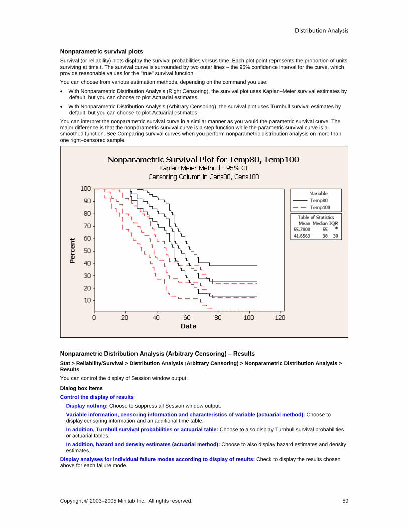
Distribution Analysis
Copyright © 2003–2005 Minitab Inc. All rights reserved. 59
Nonparametric survival plots Survival (or reliability) plots display the survival probabilities versus time. Each plot point represents the proportion of units surviving at time t. The survival curve is surrounded by two outer lines − the 95% confidence interval for the curve, which provide reasonable values for the "true" survival function. You can choose from various estimation methods, depending on the command you use:
• With Nonparametric Distribution Analysis (Right Censoring), the survival plot uses Kaplan−Meier survival estimates by default, but you can choose to plot Actuarial estimates.
• With Nonparametric Distribution Analysis (Arbitrary Censoring), the survival plot uses Turnbull survival estimates by default, but you can choose to plot Actuarial estimates.
You can interpret the nonparametric survival curve in a similar manner as you would the parametric survival curve. The major difference is that the nonparametric survival curve is a step function while the parametric survival curve is a smoothed function. See Comparing survival curves when you perform nonparametric distribution analysis on more than one right−censored sample.
Nonparametric Distribution Analysis (Arbitrary Censoring) − Results Stat > Reliability/Survival > Distribution Analysis (Arbitrary Censoring) > Nonparametric Distribution Analysis > Results You can control the display of Session window output.
Dialog box items Control the display of results
Display nothing: Choose to suppress all Session window output. Variable information, censoring information and characteristics of variable (actuarial method): Choose to display censoring information and an additional time table. In addition, Turnbull survival probabilities or actuarial table: Choose to also display Turnbull survival probabilities or actuarial tables. In addition, hazard and density estimates (actuarial method): Choose to also display hazard estimates and density estimates.
Display analyses for individual failure modes according to display of results: Check to display the results chosen above for each failure mode.

Reliability and Survivial Analysis
Copyright © 2003–2005 Minitab Inc. All rights reserved. 60
Nonparametric Distribution Analysis (Arbitrary Censoring) − Storage Stat > Reliability/Survival > Distribution Analysis (Arbitrary Censoring) > Nonparametric Distribution Analysis > Storage You can store various probability and rate estimates.
Dialog box items Enter number of levels in by variable: If all of the samples are stacked in one column, enter the number of levels the column of grouping indicators contains. Nonparametric estimates Check any of the items below to store them in the worksheet.
Times for probabilities: Check to store times for survival probabilities and cumulative failure probabilities. Survival probabilities: Check to store survival probabilities. Standard error for survival probabilities: Check to store standard errors for survival probabilities. Confidence limits for survival probabilities: Check to store confidence limits for survival probabilities. Cumulative failure probabilities: Check to store cumulative failure probabilities. Standard error for cumulative failure probabilities: Check to store standard errors for cumulative failure probabilities. Confidence limits for cumulative failure probabilities: Check to store confidence limits for cumulative failure probabilities. Hazard rates: Check to store the hazard estimates. Available when you choose the Actuarial estimation method. Times for hazard rates: Check to store the times for the hazard estimates. Available when you choose the Actuarial estimation method.
Example of nonparametric distribution analysis with arbitrarily censored data Suppose you work for a company that manufactures tires. You are interested in finding out how likely it is that a tire will "fail," or wear down to 2/32 of an inch of tread, within given mileage intervals. You are especially interested in knowing how many of the tires last past 45,000 miles. You inspect each good tire at regular intervals (every 10,000 miles) to see if the tire fails, then enter the data into the Minitab worksheet. 1 Open the worksheet TIREWEAR.MTW.
2 Choose Stat > Reliability/Survival > Distribution Analysis (Arbitrary Censoring) > Nonparametric Distribution Analysis.
3 In Start variables, enter Start. In End variables, enter End. 4 In Frequency columns, enter Freq, then click OK.
Session window output
Distribution Analysis, Start = Start and End = End Variable Start: Start End: End Frequency: Freq Censoring Information Count Right censored value 71 Interval censored value 694 Left censored value 8 Turnbull Estimates Interval Probability Standard Lower Upper of Failure Error * 10000 0.010349 0.0036400 10000 20000 0.012937 0.0040644 20000 30000 0.018111 0.0047964 30000 40000 0.032342 0.0063628 40000 50000 0.047865 0.0076784 50000 60000 0.112549 0.0113672 60000 70000 0.187581 0.0140409 70000 80000 0.298836 0.0164640 80000 90000 0.187581 0.0140409 90000 * 0.091850 *

Distribution Analysis
Copyright © 2003–2005 Minitab Inc. All rights reserved. 61
Survival Standard 95.0% Normal CI Time Probability Error Lower Upper10000 0.989651 0.0036400 0.982516 0.99678520000 0.976714 0.0054243 0.966083 0.98734530000 0.958603 0.0071650 0.944560 0.97264640000 0.926261 0.0093999 0.907838 0.94468550000 0.878396 0.0117552 0.855356 0.90143660000 0.765847 0.0152311 0.735995 0.79570070000 0.578266 0.0177621 0.543453 0.61307980000 0.279431 0.0161393 0.247798 0.31106390000 0.091850 0.0103879 0.071490 0.112210
Interpreting the results The Turnbull Estimates table displays the probabilities of failure. For example, 18.76% of the tires are estimated to fail between 60,000 and 70,000 miles. You can see in the column of survival probabilities that 92.63% of the tires are estimated to survive until 40,000 miles.
Output − Nonparametric Distribution Analysis The default output for Nonparametric Distribution Analysis depends on the estimation method you choose:
Data Default estimation method Optional estimation method Right−censored Kaplan−Meier Actuarial
Arbitrarily−censored Turnbull Actuarial
Kaplan−Meier estimates • Censoring information
• Characteristics of the variable, including the mean, its standard error and 95% confidence intervals, median, interquartile range, Q1, and Q3
• Kaplan-Meier estimates of survival probabilities and their - Standard error - 95% confidence intervals
For example,
Distribution Analysis: Temp80 Variable: Temp80 Censoring Information Count Uncensored value 37 Right censored value 13 Censoring value: Cens80 = 0 Nonparametric Estimates Characteristics of Variable Standard 95.0% Normal CI Mean(MTTF) Error Lower Upper 55.7 2.20686 51.3746 60.0254 Median = 55 IQR = * Q1 = 48 Q3 = *

Reliability and Survivial Analysis
Copyright © 2003–2005 Minitab Inc. All rights reserved. 62
Kaplan-Meier Estimates Number at Number Survival Standard 95.0% Normal CI Time Risk Failed Probability Error Lower Upper 23 50 1 0.980000 0.0197990 0.941195 1.00000 24 49 1 0.960000 0.0277128 0.905684 1.00000 27 48 2 0.920000 0.0383667 0.844803 0.99520 31 46 1 0.900000 0.0424264 0.816846 0.98315 34 45 1 0.880000 0.0459565 0.789927 0.97007 35 44 1 0.860000 0.0490714 0.763822 0.95618 37 43 1 0.840000 0.0518459 0.738384 0.94162 40 42 1 0.820000 0.0543323 0.713511 0.92649 41 41 1 0.800000 0.0565685 0.689128 0.91087 45 40 1 0.780000 0.0585833 0.665179 0.89482 46 39 1 0.760000 0.0603987 0.641621 0.87838 48 38 3 0.700000 0.0648074 0.572980 0.82702 49 35 1 0.680000 0.0659697 0.550702 0.80930 50 34 1 0.660000 0.0669925 0.528697 0.79130 51 33 4 0.580000 0.0697997 0.443195 0.71680 52 29 1 0.560000 0.0701997 0.422411 0.69759 53 28 1 0.540000 0.0704840 0.401854 0.67815 54 27 1 0.520000 0.0706541 0.381521 0.65848 55 26 1 0.500000 0.0707107 0.361410 0.63859 56 25 1 0.480000 0.0706541 0.341521 0.61848 58 24 2 0.440000 0.0701997 0.302411 0.57759 59 22 1 0.420000 0.0697997 0.283195 0.55680 60 21 1 0.400000 0.0692820 0.264210 0.53579 61 20 1 0.380000 0.0686440 0.245460 0.51454 62 19 1 0.360000 0.0678823 0.226953 0.49305 64 18 1 0.340000 0.0669925 0.208697 0.47130 66 17 1 0.320000 0.0659697 0.190702 0.44930 67 16 2 0.280000 0.0634980 0.155546 0.40445 74 13 1 0.258462 0.0621592 0.136632 0.38029
Turnbull estimates • Censoring information
• Turnbull estimates of the probability of failure and their standard errors
• Turnbull estimates of the survival probabilities and their standard errors and 95% confidence intervals For example,
Distribution Analysis, Start = Start and End = End Variable Start: Start End: End Frequency: Freq Censoring Information Count Right censored value 71 Interval censored value 694 Left censored value 8 Turnbull Estimates Interval Probability Standard Lower Upper of Failure Error * 10000 0.010349 0.0036400 10000 20000 0.012937 0.0040644 20000 30000 0.018111 0.0047964 30000 40000 0.032342 0.0063628 40000 50000 0.047865 0.0076784 50000 60000 0.112549 0.0113672 60000 70000 0.187581 0.0140409 70000 80000 0.298836 0.0164640 80000 90000 0.187581 0.0140409 90000 * 0.091850 *

Distribution Analysis
Copyright © 2003–2005 Minitab Inc. All rights reserved. 63
Survival Standard 95.0% Normal CI Time Probability Error Lower Upper10000 0.989651 0.0036400 0.982516 0.99678520000 0.976714 0.0054243 0.966083 0.98734530000 0.958603 0.0071650 0.944560 0.97264640000 0.926261 0.0093999 0.907838 0.94468550000 0.878396 0.0117552 0.855356 0.90143660000 0.765847 0.0152311 0.735995 0.79570070000 0.578266 0.0177621 0.543453 0.61307980000 0.279431 0.0161393 0.247798 0.31106390000 0.091850 0.0103879 0.071490 0.112210
Actuarial survival estimates Instead of the default Kaplan-Meier or Turnbull survival estimates, you can request Actuarial estimates in the Estimate subdialog box.
• Median residual lifetimes
• Conditional probabilities of failure
• Survival probabilities With Nonparametric Distribution Analysis-Right Censoring, you can request specific time intervals. In this example, we requested equally spaced time intervals from 0-110, in increments of 20:
Distribution Analysis: Temp80 Variable: Temp80 Censoring Information Count Uncensored value 37 Right censored value 13 Censoring value: Cens80 = 0 Nonparametric Estimates Characteristics of Variable Standard 95.0% Normal CI Median Error Lower Upper 56.1905 3.36718 49.5909 62.7900 Additional Time from Time T until 50% of Running Units Fail Proportion of Running Additional Standard 95.0% Normal CI Time T Units Time Error Lower Upper 20 1.00 36.1905 3.36718 29.5909 42.7900 40 0.84 20.0000 3.08607 13.9514 26.0486 Actuarial Table Conditional Interval Number Number Number Probability StandardLower Upper Entering Failed Censored of Failure Error 0 20 50 0 0 0.000000 0.000000 20 40 50 8 0 0.160000 0.051846 40 60 42 21 0 0.500000 0.077152 60 80 21 8 4 0.421053 0.113269 80 100 9 0 6 0.000000 0.000000 100 120 3 0 3 0.000000 0.000000

Reliability and Survivial Analysis
Copyright © 2003–2005 Minitab Inc. All rights reserved. 64
Survival Standard 95.0% Normal CI Time Probability Error Lower Upper 20 1.00000 0.0000000 1.00000 1.00000 40 0.84000 0.0518459 0.73838 0.94162 60 0.42000 0.0697997 0.28320 0.55680 80 0.24316 0.0624194 0.12082 0.36550 100 0.24316 0.0624194 0.12082 0.36550 120 0.24316 0.0624194 0.12082 0.36550
Note From the Results subdialog box, you can request additional output and display Session window output for each failure mode.
Right Censored Data Goodness-of-fit statistics Minitab displays up to two goodness−of−fit statistics to help you compare the fit of distributions.
• Anderson−Darling statistic for the maximum likelihood and least squares estimation methods.
• Pearson correlation coefficient for the least squares estimation method.
The Anderson−Darling statistic is a measure of how far the plot points fall from the fitted line in a probability plot. The statistic is a weighted squared distance from the plot points to the fitted line with larger weights in the tails of the distribution. Minitab uses an adjusted Anderson−Darling statistic, because the statistic changes when a different plot point method is used. A smaller Anderson−Darling statistic indicates that the distribution fits the data better. The Pearson correlation measures the strength of the linear relationship between the X and Y variables on a probability plot. The correlation will range between 0 and 1, with higher values indicating a better fitting distribution.
Worksheet Structure (Uncensored/Right-Censored Data) To perform reliability studies, enter a column showing the failure times of each sample. For systems with more than one cause of failure, you must also enter a column defining the failure mode. See Multiple Failure Modes (Right Censored Data).
Worksheet structure :
Singly censored data Multiply censored data
Months Censor
50 F
50 F
53 F
53 F
60 F
65 F
70 C
70 C
. .
. .
. .
and so on and so on
Months Censor
50 F
53 F
60 C
65 C
70 F
70 F
50 F
53 F
. .
. .
. .
and so on and so on
The Censor column contains the corresponding censoring indicators: F designates an actual failure; C designates a unit that was removed from the test before failure. The Censor column is optional for singly censored data, but required for multiply censored data.
Note For observations with corresponding columns of frequency, see Using frequency columns.
Singly censored data You can define the censoring in one of the following ways:
• Censoring columns − Enter two columns for each sample, one column of failure times and a corresponding column of censoring indicators. The columns for each sample must be the same length, although pairs of columns from different samples can have different lengths.

Distribution Analysis
Copyright © 2003–2005 Minitab Inc. All rights reserved. 65
Censoring indicators can be numbers or text. If you do not enter a censoring value in the Censor subdialog box, Minitab assumes the lower of the two values indicates censoring, while the higher one indicates an exact failure.
• Time Censoring − Enter a column of failure times and the time at which to begin censoring. Time censoring means that you run the study for a specified period of time. All units still running at the end time are time censored. This is known as Type I censoring on the right. In the example above, units are time censored at 70 months.
• Failure Censoring − Enter a column of failure times and the number of failures at which to begin censoring. Failure censoring means that you run the study until you observe a specified number of failures. This is known as Type II censoring on the right. You specify the number of failures at which to begin censoring. In the example above, units are failure censored at 7.
Multiply censored data You must define the censoring using censoring columns.
Using frequency columns (uncensored/right censored data) You can structure each column so that it contains individual observations (one row = one observation) or unique observations with a corresponding column of frequencies (counts). Here are the same data structured both ways:
Individual observations Frequency columns
Days Censor
140 F
150 F
150 F
150 F
150 F
151 C
151 F
151 F
. .
. .
etc. etc.
Days Censor Freq
140 F 1
150 F 4
151 C 1
151 F 35
153 F 42
161 C 1
170 F 39
199 F 1
. . .
. . .
etc. etc. etc.
Four failures at 150 days.
Frequency columns are useful for data where you have large numbers of observations with common failure and censoring times. For example, warranty data usually includes large numbers of observations with common censoring times.
Stacked vs. Unstacked data In unstacked data, each sample is in a separate column. Alternatively, you can stack all the data in one column and add a column of grouping indicators that define each sample. Like censoring indicators, grouping indicators can be numbers or text.

Reliability and Survivial Analysis
Copyright © 2003–2005 Minitab Inc. All rights reserved. 66
Here is the same data set structured both ways:
Unstacked Data Stacked Data Drug A
20 30 43 51 57 82 85 89
Drug B 2 3 6 14 24 26 27 31
Drug 20 30 43 51 57 82 85 89 2 3 6 14 24 26 27 31
Group A A A A A A A A B B B B B B B B
Note You cannot analyze more than one column of stacked data at a time, so the grouping indicators must be in one column.
Distribution ID Plot Parametric distribution analysis commands You can use all parametric distribution analysis commands for both right-censored and arbitrarily-censored data. The commands include Parametric Distribution Analysis, which performs the full analysis, and creates a Distribution ID Plot and Distribution Overview Plot. These graphs are often used before the full analysis to help choose a distribution or view summary information.
Command Description
Distribution ID Plot Right Censored Arbitrarily Censored
Draws probability plots from your choice of eleven common distributions: smallest extreme value, Weibull, 3-parameter Weibull, exponential, 2-parameter exponential, normal, lognormal, 3-parameter lognormal, logistic, loglogistic, and 3-parameter loglogistic. These plots help you determine which, if any, of the parametric distributions best fits your data.
Distribution Overview Plot Right Censored Arbitrarily Censored
Draws a probability plot, probability density function, survival plot, and hazard plot in separate regions on the same graph. These help you assess the fit of the chosen distribution and view summary graphs of your data.
Parametric Distribution Analysis Right Censored Arbitrarily Censored
Fits one of eleven common parametric distributions to your data, then uses that distribution to estimate percentiles, survival probabilities, and cumulative failure probabilities. Also draws survival, cumulative failure, hazard, and probability plots.
Distribution ID Plot (Right Censoring) Stat > Reliability/Survival > Distribution Analysis (Right Censoring) > Distribution ID Plot Use Distribution ID Plot (Right Censoring) to determine which distribution best fits your data by comparing how closely the plot points lie to the best-fit lines of a probability plot. Minitab also provides two goodness-of-fit measures to help you assess how the distribution fits your data:
• Anderson-Darling for the least squares and maximum likelihood estimation methods
• Pearson correlation coefficient for the least squares estimation method You can display up to 50 samples on each plot. All the samples display on a single plot, with different colors and symbols.
Dialog box items Variables: Enter the columns of failure times. You can enter up to 50 columns (50 different samples). Frequency columns (optional): Enter the columns of frequency data.

Distribution Analysis
Copyright © 2003–2005 Minitab Inc. All rights reserved. 67
By variable: If all of the samples are stacked in one column, check By variable, then enter a column of grouping indicators. Use all distributions: Choose to have Minitab fit all eleven distributions. Specify: Choose to fit up to four distributions.
Distribution 1: Check and choose one of eleven distributions: smallest extreme value, Weibull (default), 3-parameter Weibull, exponential, 2-parameter exponential, normal, lognormal, 3-parameter lognormal, logistic, loglogistic, or 3-parameter loglogistic. Distribution 2: Check and choose one of eleven distributions: smallest extreme value, Weibull, 3-parameter Weibull, exponential, 2-parameter exponential, normal, lognormal (default), 3-parameter lognormal, logistic, loglogistic, or 3-parameter loglogistic. Distribution 3: Check and choose one of eleven distributions: smallest extreme value, Weibull, 3-parameter Weibull, exponential (default), 2-parameter exponential, normal, lognormal, 3-parameter lognormal, logistic, loglogistic, or 3-parameter loglogistic. Distribution 4: Check and choose one of eleven distributions: smallest extreme value, Weibull, 3-parameter Weibull, exponential, 2-parameter exponential, normal (default), lognormal, 3-parameter lognormal, logistic, loglogistic, or 3-parameter loglogistic.
Distribution Analysis (Right Censored Data) If your data include exact failures or if test units do not fail before your study is over, your data are right-censored. For general information on life data and censoring, see Distribution Analysis Data. You can enter up to 50 samples per analysis. Minitab estimates the functions independently for each sample, unless you assume a common shape (Weibull) or scale (other distributions). All of the samples display on a single plot, with different colors and symbols, so you can compare the various functions between samples. Minitab can analyze systems with one cause of failure or multiple causes of failure. For systems that have more than one cause of failure, see Multiple Failure Modes (Right Censored Data). Right censored data can be:
• Singly censored − All of the test units run for the same amount of time. Units surviving at the end of the study are considered censored data. Failed units are considered exact failures. Singly censored data are more common in controlled studies.
• Multiply censored − Test units are censored at different times. Failure times are intermixed with censoring times. Multiply censored data are more common in the field, where units go into service at different times.
When your data are multiply censored, you must have a column of censoring indicators. See Worksheet Structure for more information.
Note Occasionally, you may have life data with no failures. Under certain conditions, Minitab allows you to draw conclusions based on that data. See Drawing conclusions when you have few or no failures.
To make a distribution ID plot (uncensored/right-censored data) 1 Choose Stat > Reliability/Survival > Distribution Analysis (Right Censoring) > Distribution ID Plot. 2 In Variables, enter the columns of failure times. You can enter up to 50 columns (50 different samples). 3 If you have frequency columns, enter the columns in Frequency columns. 4 If all of the samples are stacked in one column, check By variable, and enter a column of grouping indicators in the
box. 5 Do one of the following:
• Choose Use all distributions to create probability plots for all eleven distributions. • Choose Specify to create up to four probability plots with the distributions of your choice.
Note If you have no censored values, you can skip steps 6 & 7.
6 Click Censor. 7 Do one of the following, then click OK.
• For data with censoring columns: Choose Use censoring columns, then enter the censoring columns in the box. The first censoring column is paired with the first data column, the second censoring column is paired with the second data column, and so on. If you like, enter the value you use to indicate censoring in Censoring value. If you do not enter a value, Minitab uses the lowest value in the censoring column.
• For time censored data: Choose Time censor at, then enter a failure time at which to begin censoring. For example, entering 500 says that any observation from 500 time units onward is considered censored.

Reliability and Survivial Analysis
Copyright © 2003–2005 Minitab Inc. All rights reserved. 68
• For failure censored data: Choose Failure censor at, then enter a number of failures at which to begin censoring. For example, entering 150 says to make all (ordered) observations starting with the 150th observation censored, and all other observations uncensored.
8 If you like, use any of the available dialog box options, then click OK.
Censor Stat > Reliability/Survival > Distribution Analysis (Right Censoring) > distribution analysis command > Censor Allows you to designate which observations are censored.
Dialog box items Censoring Options Use censoring columns: Choose Use censoring columns, then enter the censoring columns in the box. The first censoring column is paired with the first data column, the second censoring column is paired with the second data column, and so on.
Censoring value: If you like, enter the value you use to indicate censoring in Censoring value. If you do not enter a value, Minitab uses the lowest value in the censoring column. Text values must be contained in double quotes.
Time censor at: For time censored data, choose Time censor at, then enter a failure time at which to begin censoring. For example, entering 500 says that any observation from 500 time units onward is considered censored. Failure censor at: For failure censored data, choose Failure censor at, then enter a number of failures at which to begin censoring. For example, entering 150 says to make all (ordered) observations starting with the 150th observation censored, and all other observations uncensored.
Distribution ID Plot (Right Censoring) − Options Stat > Reliability/Survival > Distribution Analysis (Right Censoring) > Distribution ID Plot > Options You can choose the method used to estimate the parameters. You can also estimate percentiles for specified percents, specify the x-axis minimum and maximum, and add your own title.
Dialog box items Estimation Method
Least Squares (failure time(X) on rank(Y)): Choose to estimate the distribution parameters using the least squares (XY) method, which are estimated by fitting a regression line to the points in a probability plot. Maximum Likelihood: Choose to estimate the distribution parameters using the maximum likelihood method, which are estimated by maximizing the likelihood function.
Estimate percentiles for these percents: Enter the additional percents for which you want to estimate percentiles. You can enter individual percents (0 < P < 100) or a column of percents. Handle tied failure times by plotting:
All points: Choose to plot the cumulative percents for each occurrence of a failure time. Maximum of tied points: Choose to plot the maximum cumulative percent of identical failure times. Average (median) of tied points: Choose to plot the median cumulative percent of identical failure times.
Show graphs of different variables or by levels: Choose to display the graphs overlaid on the same graph or on separate graphs. Minimum and Maximum X Scale
Use default values: Choose to use the default values for the minimum and maximum X scale. Use: Choose to enter your own values for the X scale minimum and maximum.
Minimum X scale: Enter a value for the minimum X scale. Maximum X scale: Enter a value for the maximum X scale.
Title: To replace the default title, type the desired text in this box.
Note To change the method for calculating probability plot points, see Tools > Options > Individual Graphs > Probability Plots.
Example of a Distribution ID Plot for right-censored data Suppose you work for a company that manufactures engine windings for turbine assemblies. Engine windings may decompose at an unacceptable rate at high temperatures. You want to know − at given high temperatures − the time at which 1% of the engine windings fail. You plan to get this information by using Parametric Distribution Analysis (Right

Distribution Analysis
Copyright © 2003–2005 Minitab Inc. All rights reserved. 69
Censoring), which requires you to specify the distribution for your data. Distribution ID Plot − Right Censoring can help you choose that distribution. First you collect failure times for the engine windings at two temperatures. In the first sample, you test 50 windings at 80° C; in the second sample, you test 40 windings at 100° C. Some of the units drop out of the test for unrelated reasons. In the Minitab worksheet, you use a column of censoring indicators to designate which times are actual failures (1) and which are censored units removed from the test before failure (0). 1 Open the worksheet RELIABLE.MTW.
2 Choose Stat > Reliability/Survival > Distribution Analysis (Right Censoring) > Distribution ID Plot. 3 In Variables, enter Temp80 Temp100. 4 Choose Specify. Leave the default distributions as Weibull, lognormal, exponential, and normal. 5 Click Censor. Choose Use censoring columns and enter Cens80 Cens100 in the box. Click OK in each dialog box.
Session window output
Distribution ID Plot: Temp80, Temp100 Results for variable: Temp80 Goodness-of-Fit Anderson-Darling Correlation Distribution (adj) Coefficient Weibull 67.606 0.986 Lognormal 67.656 0.982 Exponential 71.519 * Normal 67.589 0.987 Table of Percentiles Standard 95% Normal CI Distribution Percent Percentile Error Lower Upper Weibull 1 17.7339 2.44778 13.5305 23.2431 Lognormal 1 21.5948 2.46626 17.2638 27.0123 Exponential 1 0.737540 0.115720 0.542291 1.00309 Normal 1 15.1273 4.41131 6.48126 23.7733 Weibull 5 27.7571 2.85714 22.6859 33.9618 Lognormal 5 28.6233 2.61498 23.9307 34.2361 Exponential 5 3.76414 0.590591 2.76766 5.11939 Normal 5 27.3722 3.71588 20.0893 34.6552 Weibull 10 33.8299 2.97051 28.4812 40.1830 Lognormal 10 33.2625 2.68093 28.4020 38.9548 Exponential 10 7.73184 1.21312 5.68499 10.5156 Normal 10 33.9000 3.38602 27.2635 40.5365 Weibull 50 56.7777 2.90747 51.3558 62.7720 Lognormal 50 56.5033 3.38997 50.2348 63.5539 Exponential 50 50.8663 7.98090 37.4005 69.1804 Normal 50 56.9267 2.63143 51.7692 62.0842 Table of MTTF Standard 95% Normal CI Distribution Mean Error Lower Upper Weibull 56.6179 2.7394 51.4955 62.2497 Lognormal 61.5452 3.8295 54.4791 69.5279 Exponential 73.3846 11.5140 53.9575 99.8063 Normal 56.9267 2.6314 51.7692 62.0842

Reliability and Survivial Analysis
Copyright © 2003–2005 Minitab Inc. All rights reserved. 70
Results for variable: Temp100 Goodness-of-Fit Anderson-Darling Correlation Distribution (adj) Coefficient Weibull 17.396 0.993 Lognormal 17.281 0.988 Exponential 19.338 * Normal 17.830 0.960 Table of Percentiles Standard 95% Normal CI Distribution Percent Percentile Error Lower UpperWeibull 1 4.17857 1.35339 2.21479 7.88357Lognormal 1 6.66562 1.62573 4.13270 10.7510Exponential 1 0.461937 0.0759556 0.334673 0.637595Normal 1 -9.51233 6.17367 -21.6125 2.58784 Weibull 5 9.90287 2.28281 6.30292 15.5589Lognormal 5 11.0401 2.09791 7.60714 16.0222Exponential 5 2.35756 0.387650 1.70805 3.25405Normal 5 5.38694 5.07572 -4.56130 15.3352 Weibull 10 14.4961 2.76563 9.97371 21.0692Lognormal 10 14.4474 2.37705 10.4651 19.9453Exponential 10 4.84262 0.796264 3.50848 6.68409Normal 10 13.3297 4.56053 4.39121 22.2681 Weibull 50 39.2969 3.99440 32.1986 47.9601Lognormal 50 37.3137 4.44473 29.5444 47.1261Exponential 50 31.8587 5.23847 23.0816 43.9733Normal 50 41.3478 3.50454 34.4790 48.2166 Table of MTTF Standard 95% Normal CI Distribution Mean Error Lower Upper Weibull 42.3453 3.78311 35.5434 50.4488 Lognormal 49.0798 6.98322 37.1357 64.8656 Exponential 45.9624 7.55752 33.2997 63.4401 Normal 41.3478 3.50454 34.4790 48.2166 Distribution ID Plot for Temp80, Temp100

Distribution Analysis
Copyright © 2003–2005 Minitab Inc. All rights reserved. 71
Graph window output
Interpreting the results The points fall approximately on the straight line on the lognormal probability plot, so the lognormal distribution would be a good choice when running the parametric distribution analysis. You can also compare the Anderson-Darling goodness-of-fit values to determine which distribution best fits the data. A smaller Anderson-Darling statistic means that the distribution provides a better fit. Here, the Anderson-Darling values for the lognormal distribution are lower than the Anderson-Darling values for other distributions, thus supporting your conclusion that the lognormal distribution provides the best fit. The table of percentiles and MTTFs allow you to see how your conclusions may change with different distributions.
Output − Distribution ID Plot The default output consists of:
• Goodness-of-fit statistics for the chosen distributions
• Table of percents and their percentiles, standard errors, and 95% confidence intervals
• Table of MTTFs (mean time to failures), their standard errors, and 95% confidence intervals
• Probability plots for the chosen distributions For example,
Distribution ID Plot: Temp80 Goodness-of-Fit Anderson-Darling Correlation Distribution (adj) Coefficient Weibull 67.606 0.986 Lognormal 67.656 0.982 Exponential 71.519 * Normal 67.589 0.987
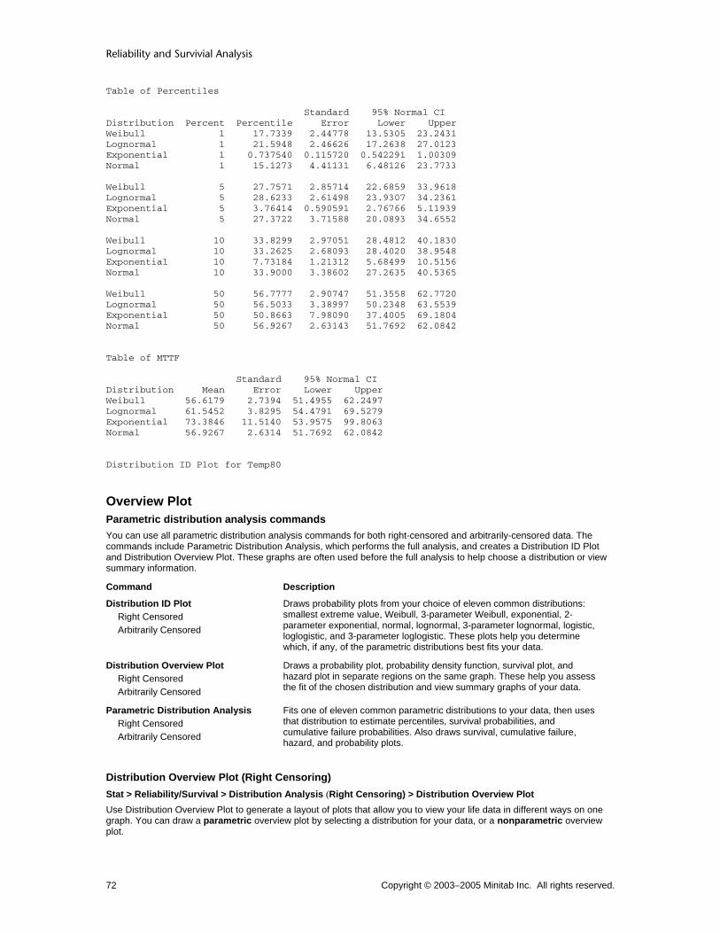
Reliability and Survivial Analysis
Copyright © 2003–2005 Minitab Inc. All rights reserved. 72
Table of Percentiles Standard 95% Normal CI Distribution Percent Percentile Error Lower UpperWeibull 1 17.7339 2.44778 13.5305 23.2431Lognormal 1 21.5948 2.46626 17.2638 27.0123Exponential 1 0.737540 0.115720 0.542291 1.00309Normal 1 15.1273 4.41131 6.48126 23.7733 Weibull 5 27.7571 2.85714 22.6859 33.9618Lognormal 5 28.6233 2.61498 23.9307 34.2361Exponential 5 3.76414 0.590591 2.76766 5.11939Normal 5 27.3722 3.71588 20.0893 34.6552 Weibull 10 33.8299 2.97051 28.4812 40.1830Lognormal 10 33.2625 2.68093 28.4020 38.9548Exponential 10 7.73184 1.21312 5.68499 10.5156Normal 10 33.9000 3.38602 27.2635 40.5365 Weibull 50 56.7777 2.90747 51.3558 62.7720Lognormal 50 56.5033 3.38997 50.2348 63.5539Exponential 50 50.8663 7.98090 37.4005 69.1804Normal 50 56.9267 2.63143 51.7692 62.0842 Table of MTTF Standard 95% Normal CI Distribution Mean Error Lower Upper Weibull 56.6179 2.7394 51.4955 62.2497 Lognormal 61.5452 3.8295 54.4791 69.5279 Exponential 73.3846 11.5140 53.9575 99.8063 Normal 56.9267 2.6314 51.7692 62.0842 Distribution ID Plot for Temp80
Overview Plot Parametric distribution analysis commands You can use all parametric distribution analysis commands for both right-censored and arbitrarily-censored data. The commands include Parametric Distribution Analysis, which performs the full analysis, and creates a Distribution ID Plot and Distribution Overview Plot. These graphs are often used before the full analysis to help choose a distribution or view summary information.
Command Description
Distribution ID Plot Right Censored Arbitrarily Censored
Draws probability plots from your choice of eleven common distributions: smallest extreme value, Weibull, 3-parameter Weibull, exponential, 2-parameter exponential, normal, lognormal, 3-parameter lognormal, logistic, loglogistic, and 3-parameter loglogistic. These plots help you determine which, if any, of the parametric distributions best fits your data.
Distribution Overview Plot Right Censored Arbitrarily Censored
Draws a probability plot, probability density function, survival plot, and hazard plot in separate regions on the same graph. These help you assess the fit of the chosen distribution and view summary graphs of your data.
Parametric Distribution Analysis Right Censored Arbitrarily Censored
Fits one of eleven common parametric distributions to your data, then uses that distribution to estimate percentiles, survival probabilities, and cumulative failure probabilities. Also draws survival, cumulative failure, hazard, and probability plots.
Distribution Overview Plot (Right Censoring) Stat > Reliability/Survival > Distribution Analysis (Right Censoring) > Distribution Overview Plot Use Distribution Overview Plot to generate a layout of plots that allow you to view your life data in different ways on one graph. You can draw a parametric overview plot by selecting a distribution for your data, or a nonparametric overview plot.
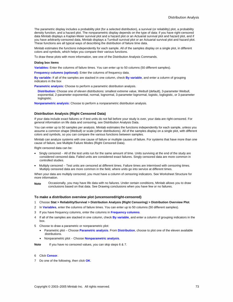
Distribution Analysis
Copyright © 2003–2005 Minitab Inc. All rights reserved. 73
The parametric display includes a probability plot (for a selected distribution), a survival (or reliability) plot, a probability density function, and a hazard plot. The nonparametric display depends on the type of data: if you have right-censored data Minitab displays a Kaplan-Meier survival plot and a hazard plot or an Actuarial survival plot and hazard plot, and if you have arbitrarily-censored data, Minitab displays a Turnbull survival plot or an Actuarial survival plot and hazard plot. These functions are all typical ways of describing the distribution of failure time data. Minitab estimates the functions independently for each sample. All of the samples display on a single plot, in different colors and symbols, which helps you compare their various functions. To draw these plots with more information, see one of the Distribution Analysis Commands.
Dialog box items Variables: Enter the columns of failure times. You can enter up to 50 columns (50 different samples). Frequency columns (optional): Enter the columns of frequency data. By variable: If all of the samples are stacked in one column, check By variable, and enter a column of grouping indicators in the box Parametric analysis: Choose to perform a parametric distribution analysis.
Distribution: Choose one of eleven distributions: smallest extreme value, Weibull (default), 3-parameter Weibull, exponential, 2-parameter exponential, normal, lognormal, 3-parameter lognormal, logistic, loglogistic, or 3-parameter loglogistic.
Nonparametric analysis: Choose to perform a nonparametric distribution analysis.
Distribution Analysis (Right Censored Data) If your data include exact failures or if test units do not fail before your study is over, your data are right-censored. For general information on life data and censoring, see Distribution Analysis Data. You can enter up to 50 samples per analysis. Minitab estimates the functions independently for each sample, unless you assume a common shape (Weibull) or scale (other distributions). All of the samples display on a single plot, with different colors and symbols, so you can compare the various functions between samples. Minitab can analyze systems with one cause of failure or multiple causes of failure. For systems that have more than one cause of failure, see Multiple Failure Modes (Right Censored Data). Right censored data can be:
• Singly censored − All of the test units run for the same amount of time. Units surviving at the end of the study are considered censored data. Failed units are considered exact failures. Singly censored data are more common in controlled studies.
• Multiply censored − Test units are censored at different times. Failure times are intermixed with censoring times. Multiply censored data are more common in the field, where units go into service at different times.
When your data are multiply censored, you must have a column of censoring indicators. See Worksheet Structure for more information.
Note Occasionally, you may have life data with no failures. Under certain conditions, Minitab allows you to draw conclusions based on that data. See Drawing conclusions when you have few or no failures.
To make a distribution overview plot (uncensored/right-censored) 1 Choose Stat > Reliability/Survival > Distribution Analysis (Right Censoring) > Distribution Overview Plot. 2 In Variables, enter the columns of failure times. You can enter up to 50 columns (50 different samples). 3 If you have frequency columns, enter the columns in Frequency columns. 4 If all of the samples are stacked in one column, check By variable, and enter a column of grouping indicators in the
box. 5 Choose to draw a parametric or nonparametric plot:
• Parametric plot − Choose Parametric analysis. From Distribution, choose to plot one of the eleven available distributions.
• Nonparametric plot − Choose Nonparametric analysis.
Note If you have no censored values, you can skip steps 6 & 7.
6 Click Censor. 7 Do one of the following, then click OK.

Reliability and Survivial Analysis
Copyright © 2003–2005 Minitab Inc. All rights reserved. 74
• For data with censoring columns: Choose Use censoring columns, then enter the censoring columns in the box. The first censoring column is paired with the first data column, the second censoring column is paired with the second data column, and so on. If you like, enter the value you use to indicate censoring in Censoring value. If you do not enter a value, Minitab uses the lowest value in the censoring column.
• For time censored data: Choose Time censor at, then enter a failure time at which to begin censoring. For example, entering 500 says that any observation from 500 time units onward is considered censored.
• For failure censored data: Choose Failure censor at, then enter a number of failures at which to begin censoring. For example, entering 150 says to censor all (ordered) observations from the 150th observed failure on, and leave all other observations uncensored.
8 If you like, use any of the available dialog box options, then click OK.
Censor Stat > Reliability/Survival > Distribution Analysis (Right Censoring) > distribution analysis command > Censor Allows you to designate which observations are censored.
Dialog box items Censoring Options Use censoring columns: Choose Use censoring columns, then enter the censoring columns in the box. The first censoring column is paired with the first data column, the second censoring column is paired with the second data column, and so on.
Censoring value: If you like, enter the value you use to indicate censoring in Censoring value. If you do not enter a value, Minitab uses the lowest value in the censoring column. Text values must be contained in double quotes.
Time censor at: For time censored data, choose Time censor at, then enter a failure time at which to begin censoring. For example, entering 500 says that any observation from 500 time units onward is considered censored. Failure censor at: For failure censored data, choose Failure censor at, then enter a number of failures at which to begin censoring. For example, entering 150 says to make all (ordered) observations starting with the 150th observation censored, and all other observations uncensored.
Distribution Overview Plot (Right Censoring) − Options Stat > Reliability/Survival > Distribution Analysis (Right Censoring) > Distribution Overview Plot > Options You can choose the method used to estimate the parameters. You can also define how ties are to be handled, specify the x-axis minimum and maximum, and add your own title.
Dialog box items Estimation Method
Least Squares (failure time(X) on rank(Y)): Choose to estimate the distribution parameters using the least squares (XY) method, which are estimated by fitting a regression line to the points in a probability plot. Maximum Likelihood: Choose to estimate the distribution parameters using the maximum likelihood method, which are estimated by maximizing the likelihood function.
Handle tied failure times by plotting: All points: Choose to plot the cumulative percents for each occurrence of a failure time. Maximum of tied points: Choose to plot the maximum cumulative percent of identical failure times. Average (median) of tied points: Choose to plot the median cumulative percent of identical failure times.
Show graphs of different variables or by levels: Choose to display the graphs overlaid on the same graph or on separate graphs. Minimum and Maximum X Scale
Use default values: Choose to use the default values for the minimum and maximum X scale. Use: Choose to enter your own values for the X scale minimum and maximum.
Minimum X scale: Enter a value for the minimum X scale. Maximum X scale: Enter a value for the maximum X scale.
Title: To replace the default title, type the desired text in this box.
Note To change the method for calculating probability plot points, see Tools > Options > Individual Graphs > Probability Plots.

Distribution Analysis
Copyright © 2003–2005 Minitab Inc. All rights reserved. 75
Example of a Distribution Overview Plot with right-censored data Suppose you work for a company that manufactures engine windings for turbine assemblies. Engine windings may decompose at an unacceptable rate at high temperatures. You want to know, at given high temperatures, at what time do 1% of the engine windings fail. You plan to get this information by using Parametric Distribution Analysis (Right Censoring), but you first want to have a quick look at your data from different perspectives. First you collect data for times to failure for the engine windings at two temperatures. In the first sample, you test 50 windings at 80° C; in the second sample, you test 40 windings at 100° C. Some of the units drop out of the test due to failures from other causes. These units are considered to be right censored because their failures were not due to the cause of interest. In the Minitab worksheet, you use a column of censoring indicators to designate which times are actual failures (1) and which are censored units removed from the test before failure (0). 1 Open the worksheet RELIABLE.MTW. 2 Choose Stat > Reliability/Survival > Distribution Analysis (Right Censoring) > Distribution Overview Plot. 3 In Variables, enter Temp80 and Temp100. 4 In Distribution, choose Lognormal. 5 Click Censor. Choose Use censoring columns and enter Cens80 and Cens100. Click OK in each dialog box.
Session window output
Distribution Overview Plot: Temp80, Temp100 Results for variable: Temp80 Goodness-of-Fit Anderson-Darling Correlation Distribution (adj) Coefficient Lognormal 67.656 0.982 Results for variable: Temp100 Goodness-of-Fit Anderson-Darling Correlation Distribution (adj) Coefficient Lognormal 17.281 0.988 Distribution Overview Plot for Temp80, Temp100

Reliability and Survivial Analysis
Copyright © 2003–2005 Minitab Inc. All rights reserved. 76
Graph window output
Interpreting the results These four plots describe the failure rate of engine windings at two different temperatures. With these plots, you can determine how much more likely it is that engine windings will fail when running at 100° C as opposed to 80° C.
Output − Distribution Overview Plot The distribution overview plot display differs depending on whether you select the parametric or nonparametric display. When you select a parametric display, you get:
• Goodness-of-fit statistics for the chosen distribution
• Probability plot, which displays estimates of the cumulative distribution function F(y) vs. failure time.
• Parametric survival (or reliability) plot, which displays the survival (or reliability) function 1-F(y) vs. failure time.
• Probability density function, which displays the curve that describes the distribution of your data, or f(y).
• Parametric hazard plot, which displays the hazard function or instantaneous failure rate, f(y)/(1-F(y)) vs. failure time. When you select a nonparametric display, you get:
• For right-censored data with Kaplan-Meier method - Kaplan-Meier survival plot - Nonparametric hazard plot based on the empirical hazard function
• For right-censored data with Actuarial method - Actuarial survival plot - Nonparametric hazard plot based on the empirical hazard function
• For arbitrarily-censored data with Turnbull method - Turnbull survival plot
• For arbitrarily-censored data with Actuarial method - Actuarial survival plot - Nonparametric hazard plot based on the empirical hazard function
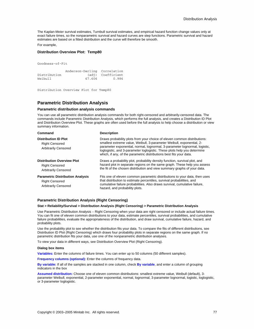
Distribution Analysis
Copyright © 2003–2005 Minitab Inc. All rights reserved. 77
The Kaplan-Meier survival estimates, Turnbull survival estimates, and empirical hazard function change values only at exact failure times, so the nonparametric survival and hazard curves are step functions. Parametric survival and hazard estimates are based on a fitted distribution and the curve will therefore be smooth. For example,
Distribution Overview Plot: Temp80 Goodness-of-Fit Anderson-Darling CorrelationDistribution (adj) CoefficientWeibull 67.606 0.986 Distribution Overview Plot for Temp80
Parametric Distribution Analysis Parametric distribution analysis commands You can use all parametric distribution analysis commands for both right-censored and arbitrarily-censored data. The commands include Parametric Distribution Analysis, which performs the full analysis, and creates a Distribution ID Plot and Distribution Overview Plot. These graphs are often used before the full analysis to help choose a distribution or view summary information.
Command Description
Distribution ID Plot Right Censored Arbitrarily Censored
Draws probability plots from your choice of eleven common distributions: smallest extreme value, Weibull, 3-parameter Weibull, exponential, 2-parameter exponential, normal, lognormal, 3-parameter lognormal, logistic, loglogistic, and 3-parameter loglogistic. These plots help you determine which, if any, of the parametric distributions best fits your data.
Distribution Overview Plot Right Censored Arbitrarily Censored
Draws a probability plot, probability density function, survival plot, and hazard plot in separate regions on the same graph. These help you assess the fit of the chosen distribution and view summary graphs of your data.
Parametric Distribution Analysis Right Censored Arbitrarily Censored
Fits one of eleven common parametric distributions to your data, then uses that distribution to estimate percentiles, survival probabilities, and cumulative failure probabilities. Also draws survival, cumulative failure, hazard, and probability plots.
Parametric Distribution Analysis (Right Censoring) Stat > Reliability/Survival > Distribution Analysis (Right Censoring) > Parametric Distribution Analysis
Use Parametric Distribution Analysis − Right Censoring when your data are right censored or include actual failure times. You can fit one of eleven common distributions to your data, estimate percentiles, survival probabilities, and cumulative failure probabilities, evaluate the appropriateness of the distribution, and draw survival, cumulative failure, hazard, and probability plots. Use the probability plot to see whether the distribution fits your data. To compare the fits of different distributions, see Distribution ID Plot (Right Censoring) which draws four probability plots in separate regions on the same graph. If no parametric distribution fits your data, use one of the nonparametric distribution analyses. To view your data in different ways, see Distribution Overview Plot (Right Censoring).
Dialog box items Variables: Enter the columns of failure times. You can enter up to 50 columns (50 different samples). Frequency columns (optional): Enter the columns of frequency data. By variable: If all of the samples are stacked in one column, check By variable, and enter a column of grouping indicators in the box Assumed distribution: Choose one of eleven common distributions: smallest extreme value, Weibull (default), 3-parameter Weibull, exponential, 2-parameter exponential, normal, lognormal, 3-parameter lognormal, logistic, loglogistic, or 3-parameter loglogistic.

Reliability and Survivial Analysis
Copyright © 2003–2005 Minitab Inc. All rights reserved. 78
Distribution Analysis (Right Censored Data) If your data include exact failures or if test units do not fail before your study is over, your data are right-censored. For general information on life data and censoring, see Distribution Analysis Data. You can enter up to 50 samples per analysis. Minitab estimates the functions independently for each sample, unless you assume a common shape (Weibull) or scale (other distributions). All of the samples display on a single plot, with different colors and symbols, so you can compare the various functions between samples. Minitab can analyze systems with one cause of failure or multiple causes of failure. For systems that have more than one cause of failure, see Multiple Failure Modes (Right Censored Data). Right censored data can be:
• Singly censored − All of the test units run for the same amount of time. Units surviving at the end of the study are considered censored data. Failed units are considered exact failures. Singly censored data are more common in controlled studies.
• Multiply censored − Test units are censored at different times. Failure times are intermixed with censoring times. Multiply censored data are more common in the field, where units go into service at different times.
When your data are multiply censored, you must have a column of censoring indicators. See Worksheet Structure for more information.
Note Occasionally, you may have life data with no failures. Under certain conditions, Minitab allows you to draw conclusions based on that data. See Drawing conclusions when you have few or no failures.
To do a parametric distribution analysis (uncensored/right censored data) 1 Choose Stat > Reliability/Survival > Distribution Analysis (Right Censoring) > Parametric Distribution
Analysis. 2 In Variables, enter the columns of failure times. You can enter up to 50 columns (50 different samples). 3 If you have frequency columns, enter the columns in Frequency columns. 4 If all of the samples are stacked in one column, check By variable, and enter a column of grouping indicators in the
box.
Note If you have no censored values, you can skip steps 5 & 6.
5 Click Censor. 6 Do one of the following, then click OK.
• For data with censoring columns: Choose Use censoring columns, then enter the censoring columns in the box. The first censoring column is paired with the first data column, the second censoring column is paired with the second data column, and so on. If you like, enter the value you used to indicate censoring in Censoring value. If you do not enter a value, by default Minitab uses the lowest value in the censoring column.
• For time censored data: Choose Time censor at, then enter a failure time at which to begin censoring. For example, entering 500 says that any observation from 500 time units onward is considered censored.
• For failure censored data: Choose Failure censor at, then enter a number of failures at which to begin censoring. For example, entering 150 says to censor all (ordered) observations from the 150th observation on, and leave all other observations uncensored.
7 If you like, use any dialog box options, then click OK.
Choosing a Distribution with a Threshold Parameter The threshold parameter, γ , provides an estimate of the earliest time a failure may occur. The threshold parameter locates the distribution along the time scale and has the same units as time, such as hours, miles, or cycles.

Distribution Analysis
Copyright © 2003–2005 Minitab Inc. All rights reserved. 79
• When γ = 0, the distribution starts at the origin.
• When γ > 0, the distribution starts to the right of the origin. The period from 0 to γ is the failure free operating period.
• When γ < 0, the distribution starts to the left of the origin. A negative γ indicates that failures have occurred prior to the beginning of a test.
Choose a distribution with a threshold parameter (3-parameter Weibull, 2-parameter exponential, 3-parameter lognormal, or 3-parameter loglogistic) when you want to estimate the earliest time-to-failure. The two probability plots show the same data fit to a Weibull and a 3-parameter Weibull distribution. The Weibull does not account for the threshold parameter and displays as a curve on probability paper. The 3-parameter Weibull adjusts for γ and the points appear straighter.
Note The threshold parameter is assumed fixed when calculating confidence intervals with the 3-parameter lognormal and 2-parameter exponential distributions.
Percentiles By what time do half of the engine windings fail? How long until 10% of the blenders stop working? You are looking for percentiles. The parametric distribution analysis commands automatically display a table of percentiles in the Session window. By default, Minitab displays the percentiles 1-10, 20, 30, 40, 50, 60, 70, 80, and 90-99. In this example, we entered failure times (in months) for engine windings.

Reliability and Survivial Analysis
Copyright © 2003–2005 Minitab Inc. All rights reserved. 80
Table of Percentiles Standard 95.0% Normal CIPercent Percentile Error Lower Upper 1 10.0765 2.78453 5.86263 17.3193 2 13.6193 3.23157 8.55426 21.6834 3 16.2590 3.48898 10.6767 24.7601 4 18.4489 3.66352 12.5009 27.2270
As shown in the first row of the table, at about 10 months (Percentile), 1% of the windings failed. The values in the Percentile column are estimates of the times at which the corresponding percent of the units failed. The table also includes standard errors and approximate 95.0% confidence intervals for each percentile. In the Estimate subdialog box, you can specify a different confidence level for all confidence intervals. You can also request percentiles to be added the default table.
Survival Probabilities − Parametric Distribution Analysis What is the probability of an engine winding running past a given time? How likely is it that a cancer patient will live five years after receiving a certain drug? You are looking for survival probabilities, which are estimates of the proportion of units that survive past a given time. When you request survival probabilities in the Estimate subdialog box, the parametric distribution analysis commands display them in the Session window. Here, for example, we requested a survival probability for engine windings running at 70 months:
Table of Survival Probabilities 95.0% Normal CI Time Probability Lower Upper 70.0000 0.4076 0.2894 0.5222
As shown in the table above, 40.76% of the engine windings last past 70 months.
Censor Stat > Reliability/Survival > Distribution Analysis (Right Censoring) > distribution analysis command > Censor Allows you to designate which observations are censored.
Dialog box items Censoring Options Use censoring columns: Choose Use censoring columns, then enter the censoring columns in the box. The first censoring column is paired with the first data column, the second censoring column is paired with the second data column, and so on.
Censoring value: If you like, enter the value you use to indicate censoring in Censoring value. If you do not enter a value, Minitab uses the lowest value in the censoring column. Text values must be contained in double quotes.
Time censor at: For time censored data, choose Time censor at, then enter a failure time at which to begin censoring. For example, entering 500 says that any observation from 500 time units onward is considered censored. Failure censor at: For failure censored data, choose Failure censor at, then enter a number of failures at which to begin censoring. For example, entering 150 says to make all (ordered) observations starting with the 150th observation censored, and all other observations uncensored.
Parametric Distribution Analysis − Failure Mode Stat > Reliability/Survival > Distribution Analysis (Right Censoring) or Distribution Analysis (Arbitrary Censoring) > Parametric Distribution Analysis > FMode Use to estimate the overall reliability of your system when multiple causes of failure exist in order to investigate the reliability of the individual failure modes. This option is available for both right-censored and arbitrarily censored data.
Dialog box items Use failure mode columns: Enter the columns containing the failure modes. To represent censored observations in the failure mode column, use an asterisk (*) for numeric columns or a space for text columns. Failure Mode Options
Use all failure modes: Choose to include all failure modes in the analysis. Use failure modes: Enter the failure modes to include in the analysis. Eliminate failure modes: Enter the failure modes to exclude from the analysis.
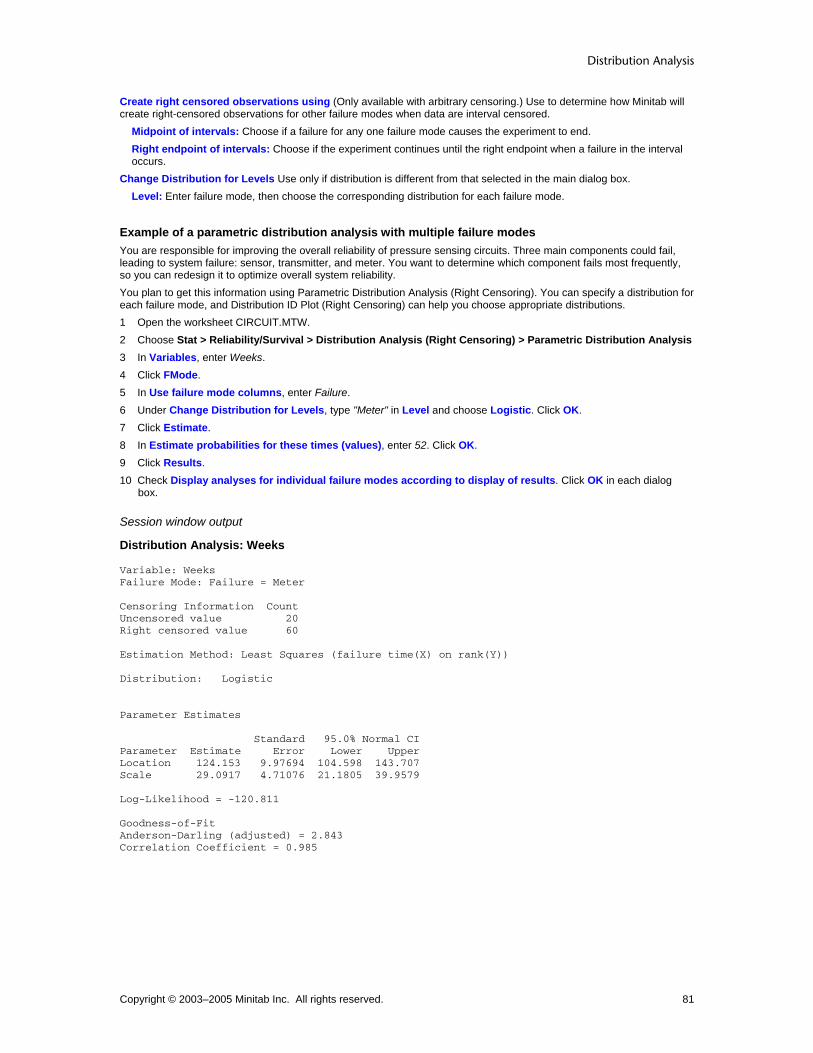
Distribution Analysis
Copyright © 2003–2005 Minitab Inc. All rights reserved. 81
Create right censored observations using (Only available with arbitrary censoring.) Use to determine how Minitab will create right-censored observations for other failure modes when data are interval censored.
Midpoint of intervals: Choose if a failure for any one failure mode causes the experiment to end. Right endpoint of intervals: Choose if the experiment continues until the right endpoint when a failure in the interval occurs.
Change Distribution for Levels Use only if distribution is different from that selected in the main dialog box. Level: Enter failure mode, then choose the corresponding distribution for each failure mode.
Example of a parametric distribution analysis with multiple failure modes You are responsible for improving the overall reliability of pressure sensing circuits. Three main components could fail, leading to system failure: sensor, transmitter, and meter. You want to determine which component fails most frequently, so you can redesign it to optimize overall system reliability. You plan to get this information using Parametric Distribution Analysis (Right Censoring). You can specify a distribution for each failure mode, and Distribution ID Plot (Right Censoring) can help you choose appropriate distributions. 1 Open the worksheet CIRCUIT.MTW. 2 Choose Stat > Reliability/Survival > Distribution Analysis (Right Censoring) > Parametric Distribution Analysis 3 In Variables, enter Weeks. 4 Click FMode. 5 In Use failure mode columns, enter Failure. 6 Under Change Distribution for Levels, type "Meter" in Level and choose Logistic. Click OK. 7 Click Estimate. 8 In Estimate probabilities for these times (values), enter 52. Click OK. 9 Click Results. 10 Check Display analyses for individual failure modes according to display of results. Click OK in each dialog
box.
Session window output
Distribution Analysis: Weeks Variable: Weeks Failure Mode: Failure = Meter Censoring Information Count Uncensored value 20 Right censored value 60 Estimation Method: Least Squares (failure time(X) on rank(Y)) Distribution: Logistic Parameter Estimates Standard 95.0% Normal CI Parameter Estimate Error Lower Upper Location 124.153 9.97694 104.598 143.707 Scale 29.0917 4.71076 21.1805 39.9579 Log-Likelihood = -120.811 Goodness-of-Fit Anderson-Darling (adjusted) = 2.843 Correlation Coefficient = 0.985

Reliability and Survivial Analysis
Copyright © 2003–2005 Minitab Inc. All rights reserved. 82
Characteristics of Distribution Standard 95.0% Normal CI Estimate Error Lower UpperMean(MTTF) 124.153 9.97694 104.598 143.707Standard Deviation 52.7666 8.54438 38.4172 72.4756Median 124.153 9.97694 104.598 143.707First Quartile(Q1) 92.1924 8.88367 74.7807 109.604Third Quartile(Q3) 156.113 13.1805 130.280 181.947Interquartile Range(IQR) 63.9211 10.3506 46.5383 87.7965 Table of Percentiles Standard 95.0% Normal CI Percent Percentile Error Lower Upper 0.1 -76.7765 29.3278 -134.258 -19.2951 1 -9.52708 19.2312 -47.2195 28.1653 2 10.9331 16.3624 -21.1366 43.0028 3 23.0272 14.7545 -5.89101 51.9454 4 31.6978 13.6581 4.92846 58.4672 5 38.4941 12.8407 13.3268 63.6614 6 44.1060 12.1993 20.1957 68.0162 7 48.9016 11.6794 26.0104 71.7929 8 53.1008 11.2485 31.0542 75.1474 9 56.8453 10.8856 35.5098 78.1807 10 60.2318 10.5767 39.5018 80.9619 20 83.8232 9.07580 66.0350 101.611 30 99.5036 8.88319 82.0928 116.914 40 112.357 9.25702 94.2138 130.501 50 124.153 9.97694 104.598 143.707 60 135.949 10.9856 114.417 157.480 70 148.802 12.3301 124.636 172.969 80 164.483 14.2128 136.626 192.339 90 188.074 17.3632 154.043 222.105 91 191.461 17.8370 156.501 226.420 92 195.205 18.3656 159.209 231.201 93 199.404 18.9640 162.235 236.573 94 204.200 19.6538 165.679 242.721 95 209.812 20.4690 169.693 249.930 96 216.608 21.4663 174.535 258.681 97 225.279 22.7524 180.685 269.873 98 237.373 24.5679 189.221 285.525 99 257.833 27.6836 203.574 312.092 Table of Survival Probabilities 95.0% Normal CI Time Probability Lower Upper 52 0.922741 0.847471 0.962510 Distribution Analysis: Weeks Variable: Weeks Failure Mode: Failure = Sensor Censoring Information Count Uncensored value 30 Right censored value 50 Estimation Method: Least Squares (failure time(X) on rank(Y)) Distribution: Weibull

Distribution Analysis
Copyright © 2003–2005 Minitab Inc. All rights reserved. 83
Parameter Estimates Standard 95.0% Normal CI Parameter Estimate Error Lower Upper Shape 2.76775 0.234031 2.34505 3.26664 Scale 99.1759 5.69945 88.6113 111.000 Log-Likelihood = -184.235 Goodness-of-Fit Anderson-Darling (adjusted) = 91.425 Correlation Coefficient = 0.984 Characteristics of Distribution Standard 95.0% Normal CI Estimate Error Lower UpperMean(MTTF) 88.2730 5.20180 78.6444 99.0805Standard Deviation 34.4842 2.39714 30.0919 39.5176Median 86.8751 5.49793 76.7409 98.3477First Quartile(Q1) 63.2279 5.18047 53.8477 74.2421Third Quartile(Q3) 111.599 5.99719 100.442 123.994Interquartile Range(IQR) 48.3708 3.36804 42.2002 55.4436 Table of Percentiles Standard 95.0% Normal CI Percent Percentile Error Lower Upper 0.1 8.17657 1.98116 5.08543 13.1467 1 18.8185 3.27552 13.3791 26.4694 2 24.2183 3.72493 17.9152 32.7388 3 28.0910 3.99019 21.2646 37.1087 4 31.2260 4.17628 24.0255 40.5844 5 33.9114 4.31797 26.4217 43.5241 6 36.2891 4.43125 28.5651 46.1016 7 38.4409 4.52483 30.5211 48.4159 8 40.4188 4.60396 32.3316 50.5291 9 42.2581 4.67210 34.0252 52.4832 10 43.9840 4.73159 35.6227 54.3079 20 57.6828 5.08268 48.5337 68.5566 30 68.3345 5.25677 58.7705 79.4549 40 77.8043 5.37997 67.9431 89.0968 50 86.8751 5.49793 76.7409 98.3477 60 96.0923 5.64198 85.6467 107.812 70 106.055 5.84987 95.1880 118.164 80 117.782 6.19298 106.248 130.567 90 134.053 6.88597 121.214 148.252 91 136.237 6.99962 123.187 150.671 92 138.609 7.12855 125.318 153.309 93 141.213 7.27683 127.647 156.220 94 144.117 7.45040 130.230 159.485 95 147.424 7.65842 133.153 163.225 96 151.301 7.91618 136.555 167.640 97 156.054 8.25215 140.690 173.095 98 162.347 8.72977 146.107 180.391 99 172.203 9.54882 154.468 191.973 Table of Survival Probabilities 95.0% Normal CI Time Probability Lower Upper 52 0.845809 0.755073 0.905001

Reliability and Survivial Analysis
Copyright © 2003–2005 Minitab Inc. All rights reserved. 84
Distribution Analysis: Weeks Variable: Weeks Failure Mode: Failure = Transmitter Censoring Information Count Uncensored value 30 Right censored value 50 Estimation Method: Least Squares (failure time(X) on rank(Y)) Distribution: Weibull Parameter Estimates Standard 95.0% Normal CI Parameter Estimate Error Lower Upper Shape 1.72088 0.181461 1.39957 2.11596 Scale 103.535 9.20506 86.9775 123.244 Log-Likelihood = -187.488 Goodness-of-Fit Anderson-Darling (adjusted) = 182.549 Correlation Coefficient = 0.987 Characteristics of Distribution Standard 95.0% Normal CI Estimate Error Lower UpperMean(MTTF) 92.3038 8.17112 77.6011 109.792Standard Deviation 55.2711 7.14057 42.9072 71.1978Median 83.6738 7.84373 69.6300 100.550First Quartile(Q1) 50.1951 6.15160 39.4770 63.8233Third Quartile(Q3) 125.175 11.1735 105.084 149.107Interquartile Range(IQR) 74.9798 8.75168 59.6474 94.2534 Table of Percentiles Standard 95.0% Normal CI Percent Percentile Error Lower Upper 0.1 1.87034 0.824159 0.788576 4.43608 1 7.14758 2.16923 3.94300 12.9566 2 10.7242 2.81901 6.40640 17.9521 3 13.6138 3.25814 8.51657 21.7618 4 16.1392 3.59506 10.4297 24.9741 5 18.4292 3.86991 12.2114 27.8130 6 20.5514 4.10256 13.8970 30.3922 7 22.5464 4.30450 15.5085 32.7783 8 24.4412 4.48302 17.0606 35.0147 9 26.2546 4.64307 18.5641 37.1312 10 28.0006 4.78821 20.0266 39.1494 20 43.3062 5.79410 33.3169 56.2905 30 56.8738 6.47457 45.5000 71.0909 40 70.0751 7.10925 57.4391 85.4909 50 83.6738 7.84373 69.6300 100.550 60 98.4064 8.81472 82.5614 117.292 70 115.327 10.2130 96.9509 137.186 80 136.516 12.4098 114.237 163.140 90 168.100 16.5175 138.653 203.801 91 172.528 17.1633 141.965 209.671 92 177.383 17.8892 145.568 216.150 93 182.773 18.7163 149.537 223.397 94 188.857 19.6753 153.976 231.639 95 195.875 20.8139 159.049 241.229 96 204.226 22.2113 165.019 252.747 97 214.642 24.0159 172.375 267.272 98 228.733 26.5584 182.177 287.185 99 251.475 30.8855 197.676 319.917

Distribution Analysis
Copyright © 2003–2005 Minitab Inc. All rights reserved. 85
Table of Survival Probabilities 95.0% Normal CI Time Probability Lower Upper 52 0.736598 0.632389 0.815503 Distribution Analysis: Weeks Variable: Weeks Failure Mode: Failure = Meter, Sensor, Transmitter Censoring Information Count Uncensored value 80 Estimation Method: Least Squares (failure time(X) on rank(Y)) Distribution: Logistic, Weibull, Weibull Table of Percentiles 95.0% Normal CI Percent Percentile Lower Upper 0.1 -76.7766 -134.258 -19.2951 1 -9.52708 -47.2195 9.27227 2 4.18134 -16.9494 12.6968 3 7.72617 0.293470 15.1079 4 10.3707 4.35150 17.4591 5 12.5881 6.77289 19.6042 6 14.5404 8.74528 21.5580 7 16.3074 10.4731 23.3531 8 17.9356 12.0401 25.0185 9 19.4550 13.4906 26.5768 10 20.8862 14.8514 28.0459 20 32.4556 25.8527 39.8636 30 41.6745 34.7026 49.1932 40 49.9792 42.7293 57.5579 50 57.9891 50.5031 65.6076 60 66.1511 58.4426 73.8054 70 74.9700 67.0254 82.6733 80 85.3122 77.0704 93.1127 90 99.5548 90.8017 107.623 91 101.456 92.6213 109.576 92 103.518 94.5891 111.698 93 105.778 96.7417 114.032 94 108.296 99.1316 116.639 95 111.157 101.838 119.614 96 114.506 104.993 123.110 97 118.605 108.832 127.411 98 124.023 113.870 133.136 99 132.500 121.669 142.180 Table of Survival Probabilities 95.0% Normal CI Time Probability Lower Upper 52 0.574887 0.480067 0.664499

Reliability and Survivial Analysis
Copyright © 2003–2005 Minitab Inc. All rights reserved. 86
Graph window output
Interpreting the results The overall 52-week circuit reliability is 0.574887. That is, 57% of the circuits survive past 52 weeks. You are 95% confident that the true reliability is between 0.480067 and 0.664499. The 52-week survival probability for each of the components is: meter, 0.922741; sensor, 0.845809; and transmitter, 0.736598. That is, 92%, 84%, and 74% of the meters, sensors, and transmitters respectively survive past 52 weeks. To improve the overall reliability, you may need to improve both the sensor and the transmitter.
Parametric Distribution Analysis − Estimate Stat > Reliability/Survival > Distribution Analysis (Right Censoring) or Distribution Analysis (Arbitrary Censoring) > Parametric Distribution Analysis > Estimate Choose the estimation used to estimate percentiles and survival probabilities for specified values. For more information on selecting estimation methods, see Least squares estimates versus maximum likelihood estimates. You can also enter a confidence level that Minitab will use for all confidence intervals.
Dialog box items Estimation Method
Least Squares (failure time(X) on rank(Y)): Choose to estimate the distribution parameters using the least squares (XY) method, which fits a regression line to the points in a probability plot. Maximum Likelihood: Choose to estimate the distribution parameters using the maximum likelihood method, which maximizes the likelihood function.
Assume common shape (slope−Weibull) or scale (1/slope−other dists): Check to estimate the parameters while assuming a common shape or scale parameter. Bayes analysis
Set shape (slope−Weibull) or scale (1/slope−other dists) at: Enter a value for the shape or scale parameter for all the response variables, or enter a list of values for the shape or scale that is equal in length to the number of variables. Set threshold at: Enter a value for the threshold parameter for all the variables, or enter a list of values equal to the number of response variables. Minitab estimates threshold parameters if you do not provide values to use.
Estimate percentiles for these additional percents: Enter the additional percents for which you want to estimate percentiles. You can enter individual percents (0 < P < 100) or a column of percents.
Distribution Analysis
Copyright © 2003–2005 Minitab Inc. All rights reserved. 87
Estimate probabilities for these times (values): Enter one or more times or a column of times for which you want to calculate survival probabilities or cumulative failure probabilities.
Estimate survival probabilities: Choose to estimate survival probabilities. Estimate cumulative failure probabilities: Choose to estimate cumulative failure probabilities.
Confidence level: Enter a confidence level for all of the confidence intervals. The default is 95.0%. Confidence intervals: Choose to use two-sided confidence intervals (the default) or just an upper or lower confidence interval.
To choose the method for estimating parameters 1 In the main dialog box, click Estimate. 2 Under Estimation Method, choose Least Squares (the default) or Maximum Likelihood. 3 Click OK.
To estimate one parameter while keeping the other parameter fixed 1 In the main dialog box, click Estimate. 2 Do one of the following:
For all distributions: • To estimate the scale parameter while keeping the shape fixed (Weibull); In Set shape (slope−Weibull) or scale
(1/slope−other dists) at, enter one value to be used for all samples, or a series of values, see Starting estimates for more information.
• To estimate the location parameter while keeping the scale fixed (other distributions); In Set shape (slope−Weibull) or scale (1/slope−other dists) at, enter one value to be used for all samples, or a series of values, see Starting estimates for more information.
For distributions with threshold parameter: • To estimate the scale and threshold parameters while keeping the shape fixed; In Set shape (slope−Weibull) or
scale (1/slope−other dists) at, enter one value to be used for all samples, or a series of values, see Starting estimates for more information.
• To estimate the scale and shape parameters while keeping the threshold fixed; In Set threshold at, enter one value to be used for all samples, or a series of values.
3 Click OK.
To request parametric survival probabilities 1 In the main dialog box, click Estimate. 2 In Estimate probabilities for these times (values), enter one or more times, or a column of times for which you want
to calculate survival probabilities. 3 Click OK.
To request additional percentiles 1 In the main dialog box, click Estimate. 2 In Estimate percentiles for these additional percents, enter the additional percents for which you want to estimate
percentiles. You can enter individual percents (0 < P < 100) or a column of percents. 3 Click OK.
To change confidence levels 1 In the main dialog box, click Estimate. 2 In Confidence level, enter a value. 3 Click OK.
To draw conclusions when you have few or no failures 1 In the main dialog box, click Estimate. 3 Under Estimation Method, choose Maximum Likelihood. 2 Depending on your distribution, under Bayes Analysis:

Reliability and Survivial Analysis
Copyright © 2003–2005 Minitab Inc. All rights reserved. 88
• In Set shape (slope−Weibull) or scale (1/slope−other dists) at, enter the shape or scale value. • In Set threshold at, enter the threshold value.
3 Click OK. For more information, see Drawing conclusions when you have few or no failures.
Least squares estimates versus maximum likelihood estimates Least squares estimates are calculated by fitting a regression line to the points in a probability plot. The line is formed by regressing time to failure or log (time to failure) (X) on the transformed percent (Y). Maximum likelihood estimates are calculated by maximizing the likelihood function. The likelihood function describes, for each set of distribution parameters, the chance that the true distribution has the parameters based on the sample. Here are the major advantages of each method:
Least squares (LSXY) • Better graphical display to the probability plot because the line is fitted to the points on a probability plot.
• For small or heavily censored sample, LSXY is more accurate than MLE. MLE tends to overestimate the shape parameter for a Weibull distribution and underestimate the scale parameter in other distributions. Therefore, MLE will tend to overestimate the low percentiles.
Maximum likelihood (MLE) • Distribution parameter estimates are more precise than least squares (XY).
• MLE allows you to perform an analysis when there are no failures. When there is only one failure and some right-censored observations, the maximum likelihood parameter estimates may exist for a Weibull distribution.
• The maximum likelihood estimation method has attractive mathematical qualities.
When possible, both methods should be tried; if the results are consistent, then there is more support for your conclusions. Otherwise, you may want to use the more conservative estimates or consider the advantages of both approaches and make a choice for your problem.
Estimating the distribution parameters You can choose to estimate the parameters using either the least squares (XY) method or the maximum likelihood method (modified Newton-Raphson algorithm). Or, if you like, you can set your own parameters. In this case, no estimation is done; all results − such as the percentiles − are based on the parameters you enter. Least squares estimates are calculated by fitting a regression line to the points in a probability plot. The line is formed by regressing time to failure or log (time to failure) (X) on the transformed percent (Y). When Minitab estimates the parameters using the maximum likelihood method, you can:
• Enter starting values for the algorithm. The maximum likelihood solution may not converge if the starting estimates are not in the neighborhood of the true solution. You may want to enter reasonable starting values for parameter estimates: − For Weibull, enter shape and scale. − For exponential, enter mean. − For other 2-parameter distributions, enter location and scale. − For 2-parameter exponential, enter scale and threshold. − For 3-parameter Weibull, enter shape, scale, and threshold. − For other 3-parameter distributions, enter location, scale, and threshold.
• Change the maximum number of iterations for reaching convergence (the default is 20). Minitab obtains maximum likelihood estimates through an iterative process. If the maximum number of iterations is reached before convergence, the algorithm terminates.
When you set historical parameters, you can fix all parameter or you can estimate at least one parameter. Estimate at least one parameter by:
− Fixing the shape OR scale − Fixing the threshold − Fixing the shape OR scale AND threshold
Drawing conclusions when you have few or no failures When you have few or no failures, you can use historical values for distribution parameters to improve your analysis. Providing historical parameters makes the resulting analysis more precise, if your values are an appropriate choice.
Distribution Analysis
Copyright © 2003–2005 Minitab Inc. All rights reserved. 89
If your data come from a Weibull or exponential distribution, you can do a Bayes analysis to obtain lower confidence bounds for parameters, percentiles, survival probabilities, and cumulative failure probabilities. If you collect life data and have no failures, Minitab can still analyze when all of the following are met:
• The data come from a Weibull or exponential distribution.
• The data are right-censored.
• The maximum likelihood method will be used to estimate parameters.
• You provide a historical value for the shape parameter (Weibull). If your data are from an exponential distribution, Minitab automatically assigns a shape parameter of 1.
Note If your data come from a three−parameter Weibull or two−parameter exponential, you must also provide a historical value for the threshold parameter.
For example, your reliability specifications require that the 5th percentile is at least 12 months. You run a Bayes analysis on data with no failures, and then examine the lower confidence bound to substantiate that the product is at least as good as specifications require. If the lower confidence bound for the 5th percentile is 13.1 months, you conclude that your product meets specifications and terminate the test. See Demonstration Test Plans to determine the optimal testing time or number of test units to use.
Parametric Distribution Analysis − Test Stat > Reliability/Survival > Distribution Analysis (Right Censoring) or Distribution Analysis (Arbitrary Censoring) > Parametric Distribution Analysis > Test Tests whether distribution parameters for a sample equal specified values, and whether two or more samples share the same shape, scale, location, or threshold parameters. Minitab performs Wald Tests [7] and provides Bonferroni 95.0% confidence intervals for the following hypothesis tests:
• Whether the distribution parameters (scale, shape, location, or threshold) are consistent with specified values
• Whether the sample comes from the historical distribution
• Whether two or more samples come from the same population
• Whether two or more samples share the same shape, scale, location, or threshold parameters
Dialog box items Consistency of Sample with Value
Test shape (slope−Weibull) or scale (1/slope−other dists) equal to: Enter a test value to compare the sample's shape (Weibull) or scale (other distributions). Test scale (Weibull or expo) or location (other dists) equal to: Enter a test value to compare the sample's scale (Weibull or exponential) or location (other distributions). Test threshold equal to: Enter a test value to compare the sample's threshold.
Equality of Parameters
Test for equal shape (slope−Weibull) or scale (1/slope−other distributions): Check to test whether two or more samples have the same shape or scale. Test for equal scale (Weibull or expo) or location (other distributions): Check to test whether two or more samples have the same scale or location. Test for equal threshold: Check to test whether two or more samples have the same threshold.
Note For 2-parameter distributions, check the first two Equality of Parameters options to test whether two or more samples come from the same population. For 3-parameter distributions, check all Equality of Parameters options, to test the same.
To compare distribution parameters to a specified value 1 In the main dialog box, click Test. 2 Do one or more of the following:
• In Test shape (slope−Weibull) or scale (1/slope−other dists) equal to, enter the test value. • In Test scale (Weibull or expo) or location (other dists) equal to, enter the test value. • In Test threshold equal to, enter the test value.
3 Click OK.

Reliability and Survivial Analysis
Copyright © 2003–2005 Minitab Inc. All rights reserved. 90
To compare parameters from two or more distributions 1 In the main dialog box, click Test. 2 Do one or more of the following:
• Check Test for equal shape (slope−Weibull) or scale (1/slope−other distributions). • Check Test for equal scale (Weibull or expo) or location (other distributions). • Check Test for equal threshold.
3 Click OK.
To determine whether two or more samples come from the same population 1 In the main dialog box, click Test. 2 Do the following:
• Check Test for equal shape (slope−Weibull) or scale (1/slope−other dists). • Check Test for equal scale (Weibull or expo) or location (other distributions). • Check Test for equal threshold.
3 Click OK.
To test whether a sample comes from a historical distribution 1 In the main dialog box, click Test. 2 Do the following:
• In Test shape (slope−Weibull) or scale (1/slope−other dists) equal to, enter the parameter of a historical distribution.
• In Test scale (Weibull or expo) or location (other dists) equal to, enter the parameter of a historical distribution.
• In Test threshold equal to, enter the parameter of a historical distribution. 3 Click OK.
Parametric Distribution Analysis (Right Censoring) − Graphs Stat > Reliability/Survival > Distribution Analysis (Right Censoring) > Parametric Distribution Analysis > Graphs You can draw a probability plot, a survival plot, cumulative failure plot, and a hazard plot.
Dialog box items Probability plot: Check to display a probability plot. Handle tied failure times by plotting
All points: Choose to plot the cumulative percents for each occurrence of a failure time. Average (median) of tied points: Choose to plot the median cumulative percent of identical failure times. Maximum of tied points: Choose to plot the maximum cumulative percent of identical failure times.
Survival plot: Check to display a survival plot. Cumulative failure plot: Check to display a cumulative failure plot. Display confidence intervals on above plots: Check to display confidence intervals on the probability, survival, and cumulative failure plots. Hazard plot: Check to display a hazard plot. Show graphs of different variables or by levels: Choose to display the graphs overlaid on the same graph or on separate graphs. Minimum X scale: Enter a value for the minimum x-axis scale. Maximum X scale: Enter a value for the maximum x-axis scale. X axis label: To replace the default x-axis label, type the text in this box.
Note To change the method for calculating probability plot points, see Tools > Options > Individual Graphs > Probability Plots.
To draw a parametric survival plot 1 In the main dialog box, click Graphs.

Distribution Analysis
Copyright © 2003–2005 Minitab Inc. All rights reserved. 91
2 Check Survival plot. 3 If you like, do any of the following:
• Uncheck Display confidence intervals on above plots to turn off the 95.0% confidence interval. (See To change confidence levels if you want to change from 95% confidence intervals.)
• In Minimum X scale and Maximum X scale, type values for the x-axis scale. • In X axis label, enter a label for the x-axis.
4 Click OK.
To modify the default probability plot 1 In the main dialog box, click Graphs. 2 Do any of the following:
To... Do... Specify the method used to obtain the plot points
See Tools > Options > Individual Graphs > Probability Plots to choose Median Rank (Benard), Mean Rank (Herd−Johnson), modified Kaplan−Meier (Hazen), or Kaplan−Meier method.
Choose what to plot when you have tied failure times
For Parametric Distribution Analysis (Right Censoring) Under Handle tied failure times by plotting, choose All points (default), Maximum of the tied points, or Average (median) of tied points.
Turn off the 95.0% confidence interval
Uncheck Display confidence intervals on above plots.
Choose how plots are displayed
Choose Overlaid on the same graph to have multiple samples plotted on the same graph, In separate panels on the same graph to have multiple samples plotted in separate panels all on the same graph, or On separate graphs to have each plot displayed separately.
Specify a minimum and/or maximum value for the x-axis scale
In Minimum X scale or Maximum X scale, enter values for the scale minimum and maximum.
Enter a label for the x-axis In X axis label, type a label.
3 Click OK. 4 To change the confidence level for the 95.0% confidence interval to some other level, click Estimate. In Confidence
level, enter a value. Click OK. 5 To change the method used to obtain the fitted line, click Estimate. In Estimation Method, choose Least Squares
(default) or Maximum Likelihood. Click OK.
Cumulative failure plots Cumulative failure plots display the cumulative failure probabilities versus time. Each plot point represents the cumulative percentage of units failing at time t. The cumulative failure curve is surrounded by two outer lines − the approximate 95.0% confidence interval for the curve, which provide reasonable values for the "true" cumulative failure function.
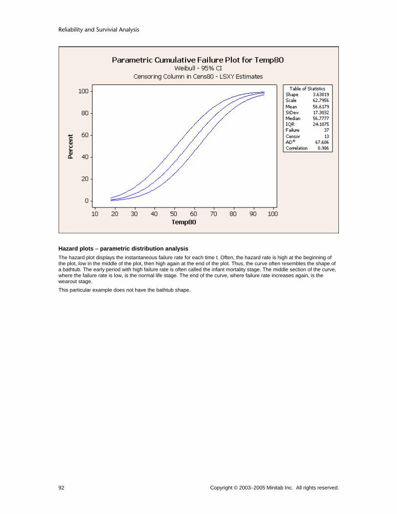
Reliability and Survivial Analysis
Copyright © 2003–2005 Minitab Inc. All rights reserved. 92
Hazard plots − parametric distribution analysis The hazard plot displays the instantaneous failure rate for each time t. Often, the hazard rate is high at the beginning of the plot, low in the middle of the plot, then high again at the end of the plot. Thus, the curve often resembles the shape of a bathtub. The early period with high failure rate is often called the infant mortality stage. The middle section of the curve, where the failure rate is low, is the normal life stage. The end of the curve, where failure rate increases again, is the wearout stage. This particular example does not have the bathtub shape.

Distribution Analysis
Copyright © 2003–2005 Minitab Inc. All rights reserved. 93
To draw a parametric hazard plot, check Hazard plot in the Graphs subdialog box.
Probability plots Use a probability plot to assess whether a particular distribution fits your data. The plot consists of:
• Plot points, which represent the proportion of failures up to a certain time. Minitab calculates the plot points using a nonparametric method. The observed failure times are plotted on the x-axis vs. the estimated cumulative probabilities (p) on the y-axis. Transformations of both the x and y data are needed to ensure that the plotted y values are a linear function of the plotted x values if the data are sampled from the particular distribution.
• Fitted line, which is a graphical representation of the percentiles. To make the fitted line, Minitab first calculates the percentiles for the various percents, based on the chosen distribution. The associated probabilities are then transformed and used as the y-variables. The percentiles may be transformed, depending on the distribution, and are used as the x-variables. The transformed scales, chosen to linearize the fitted line, differ depending on the distribution used.
• Confidence intervals, set of approximate 95.0% confidence intervals for the fitted line. For more information on probability plot calculations, see Methods and formulas - parametric distribution analysis. Because the plot points do not depend on any distribution, they would be the same (before being transformed) for any probability plot made. The fitted line, however, differs depending on the parametric distribution chosen. So you can use the probability plot to assess whether a particular distribution fits your data. In general, the closer the points fall to the fitted line, the better the fit. Minitab provides two goodness of fit measures to help assess how the distribution fits your data. To choose from various methods to estimate the plot points, see Tools > Options > Individual Graphs > Probability Plots. To choose from various methods to obtain the fitted line, see Parametric Distribution Analysis − Estimate.
Tip To quickly compare the fit of up to eleven different distributions at once, see Distribution ID Plot (Right Censoring) or Distribution ID Plot (Arbitrary Censoring).
The Weibull probability plot below shows failure times associated with running engine windings at a temperature of 80° C:

Reliability and Survivial Analysis
Copyright © 2003–2005 Minitab Inc. All rights reserved. 94
Survival plots Survival (or reliability) plots display the survival probabilities versus time. Each plot point represents the proportion of units surviving at time t. The survival curve is surrounded by two outer lines − the approximate 95.0% confidence interval for the curve, which provide reasonable values for the "true" survival function.

Distribution Analysis
Copyright © 2003–2005 Minitab Inc. All rights reserved. 95
Parametric Distribution Analysis − Results Stat > Reliability/Survival > Distribution Analysis (Right Censoring) or Distribution Analysis (Arbitrary Censoring) > Parametric Distribution Analysis > Results You can control the display of Session window output.
Dialog box items Control the Display of Results
Display nothing: Choose to suppress all Session window output. Variable information, censoring information, estimated parameters, log-likelihood, goodness-of-fit and tests of parameters: Choose to display censoring information and the estimation method. Minitab also displays the assumed distribution, parameter estimates, and tests of parameters. In addition, characteristics of distribution, table of percentiles and survival probabilities: Choose to also display the MTTF, standard deviation, median, quartile information, and percentiles. If you select survival probabilities in the Estimate subdialog box, Minitab also displays them.
Display analyses for individual failure modes according to display of results: Check to display the results chosen above for each failure mode. Show log-likelihood for each iteration of algorithm: Check to show the log-likelihood for each iteration of algorithm.
Parametric Distribution Analysis − Options Stat > Reliability/Survival > Distribution Analysis (Right Censoring) or Distribution Analysis (Arbitrary Censoring) > Parametric Distribution Analysis > Options You can specify whether the distribution parameters should be calculated from the data or enter your own historical estimates.
Dialog box items Estimate parameters of distribution: Choose to estimate the distribution parameters from the data (the default).
Use starting estimates: Enter starting estimates for the parameters. Enter one column of values to be used for all samples, or several columns of values that match the order in which the corresponding variables appear in the Variables box in the main dialog box. Maximum number of iterations: Enter the maximum number of iterations. The default number of iterations is 20.
Use historical estimates: Enter one column of values to be used for all samples, or several columns of values which match the order in which the corresponding variables appear in the Variables box in the main dialog box.
To control estimation of the parameters 1 In the main dialog box, click Options. 2 If Least Squares is your estimation method, choose Use historical estimates.
If Maximum Likelihood is your estimation method, choose one of the following:
• Estimate parameters of distribution, to estimate the distribution parameters from the data.
• Use historical estimates, to enter your own estimates for the distribution parameters. 3 If you choose Estimate parameters of distribution, you can do any of the following:
− In Use starting estimates, enter columns of starting values based on your data structure. See Starting estimates for more information.
− In Maximum number of iterations, enter a positive integer to specify the maximum number of iterations for estimation.
4 If you choose Use historical estimates,
− Enter columns of historical values based on your data structure. See Historical estimates for more information.
5 Click OK.
Starting estimates and historical estimates You must enter starting estimates or historical estimates for each distribution of failures each parameter you wish to estimate. Each variable, By variable group level, and failure mode represents a unique distribution that requires estimates in one single column or in separate columns. See the following table for various scenarios:

Reliability and Survivial Analysis
Copyright © 2003–2005 Minitab Inc. All rights reserved. 96
Variables with single failure modes:
Case Enter A single variable with a single failure mode. • Enter one column containing values for each parameter of your
distribution. Two or more variables, each with a single failure mode.
• Enter a single column containing values for each parameter for each variable.
• Enter one column of parameter estimates for each variable. A By variable with several group levels. • Enter a single column containing values for each parameter for
all group levels.
• Enter one column of values for each group level. If there are four group levels, enter four columns containing parameter estimates.
Variables with multiple failure modes:
Case Enter A single variable with a multiple failure modes.
• Enter a single column containing values for each parameter for each failure mode.
• Enter one column of parameter estimates for each failure mode. If there are three failure modes, enter three columns of parameter estimates.
Two or more variables, each with multiple failure modes.
• Enter a single column containing values for each parameter for each failure mode and variable.
• Enter one column of parameter estimates for each failure mode of each variable. If there are two variables with two failure modes, enter four columns of parameter estimates.
A By variable with several group levels and multiple failure modes.
• Enter a single column containing values for each parameter for each failure mode of each group level.
• Enter one column of parameter estimates for each failure mode of each group level. If there are two group levels with three failure modes each, enter six columns of parameter estimates.
Parameter estimates are assigned by failure mode then variable. Normally, the first column should contain the parameter estimates of failure mode 1, variable 1; the second column − parameter estimates of failure mode 1, variable 2, etc. If variable 2 does not have failure mode 1, the second column contains the parameter estimates of failure mode 2, variable 1.
Caution Do not enter starting estimates or historical estimates for failure modes that you have eliminated from the analysis.
Parametric Distribution Analysis − Storage Stat > Reliability/Survival > Distribution Analysis (Right Censoring) or Distribution Analysis (Arbitrary Censoring) > Parametric Distribution Analysis > Storage You can store characteristics of the fitted distribution and information on the distribution parameters in your worksheet. With multiple failure modes, you can store information pertaining to the overall distribution only.
Dialog box items Enter number of levels in by variable If all of the samples are stacked in one column, enter the number of levels the column of grouping indicators contains. Characteristics of Fitted Distribution
Percentiles: Check to store percentiles. Percents for percentiles: Check to store percents for percentiles. Standard error of percentiles: Check to store standard error of percentiles. Confidence limits for percentiles: Check to store confidence limits for percentiles. Times for probabilities: Check to store times for survival probabilities and cumulative failure probabilities. Available when you estimate survival probabilities or cumulative failure probabilities at different times. Survival probabilities: Check to store survival probabilities. Available when you estimate survival probabilities at different times. Confidence limits for survival probabilities: Check to store confidence limits for survival probabilities. Available when you estimate survival probabilities at different times.

Distribution Analysis
Copyright © 2003–2005 Minitab Inc. All rights reserved. 97
Cumulative failure probabilities: Check to store cumulative failure probabilities. Available when you estimate cumulative failure probabilities at different times. Confidence limits for cumulative failure probabilities: Check to store confidence limits for cumulative failure probabilities. Available when you estimate cumulative failure probabilities at different times.
Information on Parameters Choose to store the following when you have a single failure mode. Parameters estimates: Check to store parameter estimates. Standard error of estimates: Check to store standard error of parameter estimates. Confidence limits for parameters: Check to store confidence limits for parameters. Variance/covariance matrix: Check to store the variance / covariance matrix. Log-likelihood for last iteration: Check to store the log-likelihood ratio for the last iteration.
Example of a parametric distribution analysis with exact failure/right censored data Suppose you work for a company that manufactures engine windings for turbine assemblies. Engine windings may decompose at an unacceptable rate at high temperatures. You decide to look at failure times for engine windings at two temperatures, 80° C and 100° C. You want to find out the following information for each temperature:
• Times at which various percentages of the windings fail. You are particularly interested in the 0.1st percentile.
• Proportion of windings that survive past 70 months. You also want to draw two plots: a probability plot to see if the lognormal distribution provides a good fit for your data, and a survival plot. In the first sample, you collect failure times (in months) for 50 windings at 80° C; in the second sample, you collect failure times for 40 windings at 100° C. Some of the windings drop out of the test for unrelated reasons. In the Minitab worksheet, you use a column of censoring indicators to designate which times are actual failures (1) and which are censored units removed from the test before failure (0). 1 Open the worksheet RELIABLE.MTW. 2 Choose Stat > Reliability/Survival > Distribution Analysis (Right Censoring) > Parametric Distribution
Analysis. 3 In Variables, enter Temp80 Temp100. 4 From Assumed distribution, choose Lognormal. 5 Click Censor. Choose Use censoring columns and enter Cens80 Cens100 in the box. Click OK. 6 Click Estimate. In Estimate percentiles for these additional percents, enter 0.1. 7 In Estimate probabilities for these times (values), enter 70. Click OK. 8 Click Graphs. Check Survival plot. Click OK in each dialog box.
Session window output
Distribution Analysis: Temp80 Variable: Temp80 Censoring Information Count Uncensored value 37 Right censored value 13 Censoring value: Cens80 = 0 Estimation Method: Least Squares (failure time(X) on rank(Y)) Distribution: Lognormal Parameter Estimates Standard 95.0% Normal CI Parameter Estimate Error Lower Upper Location 4.03430 0.0599960 3.91671 4.15189 Scale 0.413458 0.0414962 0.339626 0.503340 Log-Likelihood = -182.827

Reliability and Survivial Analysis
Copyright © 2003–2005 Minitab Inc. All rights reserved. 98
Goodness-of-Fit Anderson-Darling (adjusted) = 67.656 Correlation Coefficient = 0.982 Characteristics of Distribution Standard 95.0% Normal CI Estimate Error Lower UpperMean(MTTF) 61.5452 3.82954 54.4791 69.5279Standard Deviation 26.5736 3.70119 20.2253 34.9145Median 56.5033 3.38997 50.2348 63.5539First Quartile(Q1) 42.7524 2.84200 37.5298 48.7018Third Quartile(Q3) 74.6770 4.92345 65.6247 84.9780Interquartile Range(IQR) 31.9246 3.78623 25.3031 40.2788 Table of Percentiles Standard 95.0% Normal CI Percent Percentile Error Lower Upper 0.1 15.7465 2.23848 11.9173 20.8060 1 21.5948 2.46626 17.2638 27.0123 2 24.1712 2.53192 19.6850 29.6798 3 25.9629 2.56907 21.3858 31.5197 4 27.3978 2.59497 22.7560 32.9866 5 28.6233 2.61498 23.9307 34.2361 6 29.7095 2.63147 24.9747 35.3418 7 30.6957 2.64569 25.9245 36.3448 8 31.6064 2.65838 26.8029 37.2708 9 32.4582 2.67001 27.6251 38.1368 10 33.2625 2.68093 28.4020 38.9548 20 39.8979 2.78266 34.8003 45.7422 30 45.4895 2.91315 40.1236 51.5730 40 50.8841 3.10502 45.1482 57.3487 50 56.5033 3.38997 50.2348 63.5539 60 62.7430 3.81469 55.6947 70.6834 70 70.1837 4.46368 61.9584 79.5010 80 80.0198 5.52897 69.8849 91.6244 90 95.9826 7.65393 82.0947 112.220 91 98.3610 8.00485 83.8591 115.371 92 101.012 8.40509 85.8113 118.905 93 104.009 8.86871 88.0014 122.928 94 107.461 9.41666 90.5031 127.597 95 111.539 10.0819 93.4305 133.158 96 116.528 10.9209 96.9744 140.025 97 122.968 12.0421 101.493 148.988 98 132.084 13.6963 107.792 161.851 99 147.842 16.7224 118.446 184.535 Table of Survival Probabilities 95.0% Normal CI Time Probability Lower Upper 70 0.302208 0.206353 0.414111 Distribution Analysis: Temp100 Variable: Temp100 Censoring Information Count Uncensored value 34 Right censored value 6 Censoring value: Cens100 = 0 Estimation Method: Least Squares (failure time(X) on rank(Y))

Distribution Analysis
Copyright © 2003–2005 Minitab Inc. All rights reserved. 99
Distribution: Lognormal Parameter Estimates Standard 95.0% Normal CI Parameter Estimate Error Lower Upper Location 3.61936 0.119118 3.38589 3.85283 Scale 0.740387 0.0949534 0.575829 0.951972 Log-Likelihood = -160.697 Goodness-of-Fit Anderson-Darling (adjusted) = 17.281 Correlation Coefficient = 0.988 Characteristics of Distribution Standard 95.0% Normal CI Estimate Error Lower UpperMean(MTTF) 49.0798 6.98322 37.1357 64.8656Standard Deviation 41.9364 11.4125 24.6006 71.4885Median 37.3137 4.44473 29.5444 47.1261First Quartile(Q1) 22.6459 2.97661 17.5027 29.3003Third Quartile(Q3) 61.4820 8.54241 46.8253 80.7263Interquartile Range(IQR) 38.8361 7.33100 26.8260 56.2232 Table of Percentiles Standard 95.0% Normal CI Percent Percentile Error Lower Upper 0.1 3.78631 1.17097 2.06524 6.94163 1 6.66562 1.62573 4.13270 10.7510 2 8.15631 1.80788 5.28227 12.5941 3 9.27058 1.92809 6.16701 13.9360 4 10.2080 2.02085 6.92520 15.0471 5 11.0401 2.09791 7.60714 16.0222 6 11.8015 2.16476 8.23760 16.9073 7 12.5122 2.22448 8.83086 17.7282 8 13.1848 2.27898 9.39602 18.5013 9 13.8278 2.32954 9.93927 19.2377 10 14.4474 2.37705 10.4651 19.9453 20 20.0101 2.78063 15.2393 26.2744 30 25.3075 3.18917 19.7690 32.3978 40 30.9318 3.71014 24.4516 39.1294 50 37.3137 4.44473 29.5444 47.1261 60 45.0123 5.54010 35.3643 57.2924 70 55.0158 7.26891 42.4642 71.2774 80 69.5806 10.2830 52.0826 92.9574 90 96.3710 16.9469 68.2750 136.029 91 100.689 18.1275 70.7518 143.294 92 105.600 19.5006 73.5320 151.653 93 111.276 21.1262 76.7007 161.438 94 117.978 23.0951 80.3841 173.153 95 126.114 25.5534 84.7800 187.601 96 136.394 28.7576 90.2247 206.188 97 150.186 33.2146 97.3603 231.675 98 170.704 40.1446 107.663 270.658 99 208.880 53.8572 126.016 346.233 Table of Survival Probabilities 95.0% Normal CI Time Probability Lower Upper 70 0.197736 0.107086 0.323727

Reliability and Survivial Analysis
Copyright © 2003–2005 Minitab Inc. All rights reserved. 100
Graph window output
Interpreting the results To see the times at which various percentages of the windings fail, look at the Table of Percentiles. At 80° C, for example, it takes 21.5948 months for 1% of the windings to fail.

Distribution Analysis
Copyright © 2003–2005 Minitab Inc. All rights reserved. 101
You can find the 0.1st percentile, which you requested, within the Table of Percentiles. At 80° C, 0.1% of the windings fail by 15.7465 months; at 100° C, 0.1% of the windings fail by 3.78631 months. So the increase in temperature decreased the percentile by about 9.5 months. What proportion of windings would you expect to still be running past 70 months? In the Table of Survival Probabilities you find your answer. At 80° C, 30.22% survive past 70 months; at 100° C, 19.77% survive.
Output − Parametric Distribution Analysis The default output for Parametric Distribution Analysis (Right Censoring) and Parametric Distribution Analysis (Arbitrary Censoring) is:
• Censoring information
• Parameter estimates and their - Standard errors - 95% confidence intervals - Log-likelihood and goodness-of-fit statistics
• Characteristics of distribution and their - Standard errors - 95% confidence intervals
• Table of percentiles and their - Standard errors - 95% confidence intervals
• Probability plot for each failure mode For example,
Distribution Analysis: Temp80 Variable: Temp80 Censoring Information Count Uncensored value 37 Right censored value 13 Censoring value: Cens80 = 0 Estimation Method: Least Squares (failure time(X) on rank(Y)) Distribution: Weibull Parameter Estimates Standard 95.0% Normal CI Parameter Estimate Error Lower Upper Shape 3.63819 0.296611 3.10091 4.26856 Scale 62.7956 2.84080 57.4674 68.6177 Log-Likelihood = -202.258 Goodness-of-Fit Anderson-Darling (adjusted) = 67.606 Correlation Coefficient = 0.986 Characteristics of Distribution Standard 95.0% Normal CI Estimate Error Lower UpperMean(MTTF) 56.6179 2.73936 51.4955 62.2497Standard Deviation 17.3032 0.872053 15.6757 19.0996Median 56.7777 2.90747 51.3558 62.7720First Quartile(Q1) 44.5866 3.00877 39.0629 50.8914Third Quartile(Q3) 68.6941 2.78798 63.4415 74.3817Interquartile Range(IQR) 24.1075 1.27922 21.7263 26.7498

Reliability and Survivial Analysis
Copyright © 2003–2005 Minitab Inc. All rights reserved. 102
Table of Percentiles Standard 95.0% Normal CI Percent Percentile Error Lower Upper 1 17.7339 2.44778 13.5305 23.2431 2 21.4857 2.64045 16.8866 27.3374 3 24.0525 2.74337 19.2342 30.0778 4 26.0685 2.81001 21.1039 32.2010 5 27.7571 2.85714 22.6859 33.9618 6 29.2256 2.89222 24.0728 35.4813 7 30.5348 2.91916 25.3174 36.8274 8 31.7228 2.94029 26.4531 38.0423 9 32.8152 2.95707 27.5024 39.1542 10 33.8299 2.97051 28.4812 40.1830 20 41.5795 3.01453 36.0717 47.9283 30 47.3005 2.99523 41.7796 53.5509 40 52.2089 2.95551 46.7259 58.3351 50 56.7777 2.90747 51.3558 62.7720 60 61.3046 2.85684 55.9534 67.1676 70 66.0826 2.80866 60.8008 71.8233 80 71.5708 2.77225 66.3384 77.2159 90 78.9748 2.78019 73.7094 84.6162 91 79.9520 2.78771 74.6707 85.6068 92 81.0084 2.79777 75.7063 86.6817 93 82.1636 2.81118 76.8345 87.8624 94 83.4461 2.82909 78.0814 89.1794 95 84.8988 2.85336 79.4865 90.6796 96 86.5920 2.88716 81.1142 92.4397 97 88.6536 2.93652 83.0809 94.6000 98 91.3603 3.01533 85.6375 97.4656 99 95.5499 3.16895 89.5364 101.967
Note From the Results subdialog box, you can request additional output and display Session window output for each failure mode.
Nonparametric Distribution Analysis Nonparametric distribution analysis commands The nonparametric distribution analysis commands include Nonparametric Distribution Analysis-Right Censoring and Nonparametric Distribution Analysis-Arbitrary Censoring, which perform the full analysis, and create a Distribution Overview Plot. This graph is often used before the full analysis to view summary information.
Command Description
Distribution Overview Plot Right Censored Arbitrary Censored
Draws a Kaplan-Meier survival plot and hazard plot on one graph. Draws a Turnbull survival plot, or an Actuarial survival plot and hazard plot, on one graph.
Nonparametric Distribution Analysis Right Censored Arbitrary Censored
Gives you nonparametric estimates of the survival probabilities, cumulative failure probabilities, hazard rates, and other estimates depending on the nonparametric technique chosen, and draw survival, cumulative failure, and hazard plots. When you have multiple samples, Nonparametric Distribution Analysis - Right Censoring also tests the equality of their survival curves.
Nonparametric Distribution Analysis (Right Censoring) Stat > Reliability/Survival > Distribution Analysis (Right Censoring) > Nonparametric Distribution Analysis Use this command when you have right censored data or actual failure times and no distribution fits your data. You can estimate survival probabilities, cumulative failure probabilities, hazard rates, and other functions, and draw survival, cumulative failure, and hazard plots. When you have exact failure/right-censored data, you can request Kaplan-Meier or Actuarial estimates. When you have tabled data with a varied censoring scheme, you can request Turnbull or Actuarial estimates. When you have exact failure/right-censored data and multiple samples, Minitab tests the equality of survival curves. To make a quick Kaplan-Meier survival plot and empirical hazard plot, see Distribution Overview Plot (Right Censoring).

Distribution Analysis
Copyright © 2003–2005 Minitab Inc. All rights reserved. 103
If a distribution fits your data, use Parametric Distribution Analysis (Right Censoring).
Dialog box items Variables: Enter the columns of failure times. You can enter up to 50 columns (50 different samples). Frequency columns (optional): Enter the columns of frequency data. By variable: If all of the samples are stacked in one column, check By variable, and enter a column of grouping indicators in the box
Distribution Analysis (Right Censored Data) If your data include exact failures or if test units do not fail before your study is over, your data are right-censored. For general information on life data and censoring, see Distribution Analysis Data. You can enter up to 50 samples per analysis. Minitab estimates the functions independently for each sample, unless you assume a common shape (Weibull) or scale (other distributions). All of the samples display on a single plot, with different colors and symbols, so you can compare the various functions between samples. Minitab can analyze systems with one cause of failure or multiple causes of failure. For systems that have more than one cause of failure, see Multiple Failure Modes (Right Censored Data). Right censored data can be:
• Singly censored − All of the test units run for the same amount of time. Units surviving at the end of the study are considered censored data. Failed units are considered exact failures. Singly censored data are more common in controlled studies.
• Multiply censored − Test units are censored at different times. Failure times are intermixed with censoring times. Multiply censored data are more common in the field, where units go into service at different times.
When your data are multiply censored, you must have a column of censoring indicators. See Worksheet Structure for more information.
Note Occasionally, you may have life data with no failures. Under certain conditions, Minitab allows you to draw conclusions based on that data. See Drawing conclusions when you have few or no failures.
To do a nonparametric distribution analysis (uncensored/right censored data) 1 Choose Stat > Reliability/Survival > Distribution Analysis (Right Censoring) > Nonparametric Distribution
Analysis. 2 In Variables, enter the columns of failure times. You can enter up to 50 columns (50 different samples). 3 If you have frequency columns, enter the columns in Frequency columns. 4 If all of the samples are stacked in one column, enter a column of grouping indicators in By variable.
Note If you have no censored values, you can skip steps 5 & 6.
5 Click Censor. 6 Do one of the following, then click OK.
• For data with censoring columns: Choose Use censoring columns, then enter the censoring columns in the box. The first censoring column is paired with the first data column, the second censoring column is paired with the second data column, and so on.
If you like, enter the value you use to indicate a censored value in Cens value. If you do not enter a censoring value, Minitab uses the lowest value in the censoring column by default.
• For time censored data: Choose Time censor at, then enter a failure time at which to begin censoring. For example, entering 500 says that any observation from 500 time units onward is considered censored.
• For failure censored data: Choose Failure censor at, then enter a number of failures at which to begin censoring. For example, entering 150 says to censor all (ordered) observations starting with the 150th observation censored, and leave all other observations uncensored.
7 If you like, use any of the available dialog box options, then click OK.
Censor Stat > Reliability/Survival > Distribution Analysis (Right Censoring) > distribution analysis command > Censor Allows you to designate which observations are censored.
Reliability and Survivial Analysis
Copyright © 2003–2005 Minitab Inc. All rights reserved. 104
Dialog box items Censoring Options Use censoring columns: Choose Use censoring columns, then enter the censoring columns in the box. The first censoring column is paired with the first data column, the second censoring column is paired with the second data column, and so on.
Censoring value: If you like, enter the value you use to indicate censoring in Censoring value. If you do not enter a value, Minitab uses the lowest value in the censoring column. Text values must be contained in double quotes.
Time censor at: For time censored data, choose Time censor at, then enter a failure time at which to begin censoring. For example, entering 500 says that any observation from 500 time units onward is considered censored. Failure censor at: For failure censored data, choose Failure censor at, then enter a number of failures at which to begin censoring. For example, entering 150 says to make all (ordered) observations starting with the 150th observation censored, and all other observations uncensored.
Nonparametric Distribution Analysis − Failure Mode Stat > Reliability/Survival > Distribution Analysis (Right Censoring) or Distribution Analysis (Arbitrary Censoring) > Nonparametric Distribution Analysis > FMode Use to estimate the overall reliability of your system when multiple causes of failure exist in order to investigate the reliability of the individual failure modes. This option is available for both right-censored and arbitrarily censored data.
Dialog box items Use failure mode columns: Enter the columns containing the failure modes. Failure Mode Options
Use all failure modes: Choose to include all failure modes in the analysis. Use failure modes: Enter the failure modes to include in the analysis. Eliminate failure modes: Enter the failure modes to exclude from the analysis.
Create right censored observations using (Only available with arbitrary censoring.) Use to determine how Minitab will create right-censored observations for other failure modes when data are interval censored.
Midpoint of intervals: Choose if a failure for any one failure mode causes the experiment to end. Right endpoint of intervals: Choose if the experiment continues until the right endpoint when a failure in the interval occurs.
Nonparametric Distribution Analysis (Right Censoring) − Estimate Stat > Reliability/Survival > Distribution Analysis (Right Censoring) > Nonparametric Distribution Analysis > Estimate You can choose the method of estimation for the nonparametric estimates of survival probabilities, cumulative failure probabilities, hazard rates, etc.
Dialog box items Estimation Method
Kaplan-Meier: Choose to estimate the parameters using the Kaplan-Meier method. Actuarial method: Choose to estimate the parameters using the actuarial method.
Specify time intervals as 0 to __ by __: Choose to use equally spaced time intervals − choose and enter numbers in the boxes. For example, 0 to 100 by 20 gives you these time intervals: 0-20, 20-40, and so on up to 80-100. Enter endpoints of intervals: Choose to use unequally spaced time intervals and enter a series of numbers, or a column of numbers, in the box. For example, entering 0 4 6 8 10 20 30, gives you these time intervals: 0-4, 4-6, 6-8, 8-10, 10-20, and 20-30.
Estimate survival probabilities: Choose to estimate survival probabilities. Estimate cumulative failure probabilities: Choose to estimate cumulative failure probabilities. Confidence level: Enter a confidence level for all of the confidence intervals. The default is 95.0%. Confidence intervals: Choose to use two-sided confidence intervals (the default) or just an upper or lower confidence interval.

Distribution Analysis
Copyright © 2003–2005 Minitab Inc. All rights reserved. 105
To request actuarial estimates 1 In the main dialog box, click Estimate. 2 Under Estimation Method, check Actuarial. 3 With Nonparametric Distribution Analysis (Right Censoring), do one of the following:
• use equally spaced time intervals − choose 0 to_by_ and enter numbers in the boxes. For example, 0 to 100 by 20 gives you these time intervals: 0-20, 20-40, and so on up to 80-100.
• use unequally spaced time intervals − choose Enter endpoints of intervals, and enter a series of numbers, or a column of numbers, in the box. For example, entering 0 4 6 8 10 20 30, gives you these time intervals: 0-4, 4-6, 6-8, 8-10, 10-20, and 20-30.
4 Click OK.
More To display hazard and density estimates in the Actuarial table, from the main dialog box, click Results. Do one of the following and then click :
With Nonparametric Distribution Analysis (Right Censoring), choose In addition, hazard, density (actuarial method) estimates and log-rank and Wilcoxon statistics.
With Nonparametric Distribution Analysis (Arbitrary Censoring), choose In addition, hazard and density estimates (actuarial method).
To change confidence levels 1 In the main dialog box, click Estimate. 2 In Confidence level, enter a value. 3 Click OK.
Nonparametric Distribution Analysis − Graphs Stat > Reliability/Survival > Distribution Analysis (Right Censoring) or Distribution Analysis (Arbitrary Censoring) > Nonparametric Distribution Analysis > Graphs You can draw survival plots, cumulative failure plots, and hazard plots.
Dialog box items Survival plot: Check to display a survival plot. Cumulative failure plot: Check to display a cumulative failure plot. Display confidence intervals on plot: Check to display confidence intervals on the survival and cumulative failure plots. Hazard Plots: Check to display a hazard plot. Show graphs of different variables or by levels: Choose to display the graphs overlaid on the same graph or on separate graphs. Minimum X scale: Enter a value for the minimum X-axis scale. Maximum X scale: Enter a value for the maximum X-axis scale. X axis label: To replace the default X-axis label with your own label, enter the desired text in this box.
To draw a hazard plot 1 In the Nonparametric Distribution Analysis (Right Censoring) dialog box, click Graphs. 2 Check Hazard plot. 3 If you like, use any of the available dialog box options, then click OK.
More By default, the hazard plot for Nonparametric Distribution Analysis (Right Censoring) uses the empirical hazard function. If you want to plot Actuarial estimates, choose Actuarial method in the Estimate subdialog box. See To request actuarial estimates.
Hazard plots − nonparametric distribution analysis The hazard plot displays the instantaneous failure rate for each time t. Often, the hazard rate is high at the beginning of the plot, low in the middle of the plot, then high again at the end of the plot. Thus, the curve often resembles the shape of a bathtub. The early period with high failure rate is often called the infant mortality stage. The middle section of the curve, where the failure rate is low, is the normal life stage. The end of the curve, where failure rate increases again, is the wearout stage.

Reliability and Survivial Analysis
Copyright © 2003–2005 Minitab Inc. All rights reserved. 106
Nonparametric hazard estimates are calculated various ways:
• Nonparametric Distribution Analysis (Right Censoring) automatically plots the empirical hazard function. You can optionally plot Actuarial estimates.
• Nonparametric Distribution Analysis (Arbitrary Censoring) only plots Actuarial estimates. Since the Actuarial method is not the default estimation method, be sure to choose Actuarial method in the Estimate subdialog box when you want to draw a hazard plot.
Nonparametric survival plots Survival (or reliability) plots display the survival probabilities versus time. Each plot point represents the proportion of units surviving at time t. The survival curve is surrounded by two outer lines − the 95% confidence interval for the curve, which provide reasonable values for the "true" survival function. You can choose from various estimation methods, depending on the command you use:
• With Nonparametric Distribution Analysis (Right Censoring), the survival plot uses Kaplan−Meier survival estimates by default, but you can choose to plot Actuarial estimates.
• With Nonparametric Distribution Analysis (Arbitrary Censoring), the survival plot uses Turnbull survival estimates by default, but you can choose to plot Actuarial estimates.
You can interpret the nonparametric survival curve in a similar manner as you would the parametric survival curve. The major difference is that the nonparametric survival curve is a step function while the parametric survival curve is a smoothed function. See Comparing survival curves when you perform nonparametric distribution analysis on more than one right−censored sample.

Distribution Analysis
Copyright © 2003–2005 Minitab Inc. All rights reserved. 107
Comparing survival curves (nonparametric distribution analysis-right censoring only) When you enter more than one sample, Nonparametric Distribution Analysis-Right Censoring automatically compares their survival curves, and displays this table in the Session window:
Comparison of Survival Curves Test Statistics Method Chi-Square DF P-Value Log-Rank 7.7152 1 0.0055 Wilcoxon 13.1326 1 0.0003
This table contains measures that tell you if the survival curves for various samples are significantly different. A p-value < α indicates that the survival curves are significantly different. To get more detailed log-rank and Wilcoxon statistics, choose In addition, hazard, density (actuarial method) estimates and log-rank and Wilcoxon statistics in the Results subdialog box.
Nonparametric Distribution Analysis (Right Censoring) − Results Stat > Reliability/Survival > Distribution Analysis (Right Censoring) > Nonparametric Distribution Analysis > Results You can control the display of Session window output.
Dialog box items Control the display of results
Display nothing: Choose to suppress all Session window output. Variable information, censoring information, characteristics of variable and test statistics for comparing survival curves: Choose to display censoring information and MTTF, standard deviation, median, quartile information, and test statistics for survival curves. In addition, Kaplan-Meier survival probabilities or actuarial tables: Choose to also display Kaplan-Meier survival probabilities or actuarial tables. In addition, hazard, density (actuarial methods) estimates and log-rank and Wilcoxon statistics: Choose to also display hazard estimates, density estimates, log-rank statistics, and Wilcoxon statistics.

Reliability and Survivial Analysis
Copyright © 2003–2005 Minitab Inc. All rights reserved. 108
Display analyses for individual failure modes according to display of results: Check to display the results for each failure mode.
Nonparametric Distribution Analysis (Right Censoring) − Storage Stat > Reliability/Survival > Distribution Analysis (Right Censoring) > Nonparametric Distribution Analysis > Storage You can store various probability and rate estimates.
Dialog box items Enter number of levels in by variable If all of the samples are stacked in one column, enter the number of levels the column of grouping indicators contains. Nonparametric estimates Check any of the items below to store them in the worksheet.
Times for probabilities: Check to store times for survival probabilities and cumulative failure probabilities. Survival probabilities: Check to store survival probabilities. Standard error for survival probabilities: Check to store standard errors for survival probabilities. Confidence limits for survival probabilities: Check to store confidence limits for survival probabilities. Cumulative failure probabilities: Check to store cumulative failure probabilities. Standard error for cumulative failure probabilities: Check to store standard errors for cumulative failure probabilities. Confidence limits for cumulative failure probabilities: Check to store confidence limits for cumulative failure probabilities. Hazard rates: Check to store the hazard estimates. Times for hazard rates: Check to store the times for the hazard estimates.
Example of nonparametric distribution analysis with exact failure/right censored data Suppose you work for a company that manufactures engine windings for turbine assemblies. Engine windings may decompose at an unacceptable rate at high temperatures. You decide to look at failure times for engine windings at two temperatures, 80° C and 100° C. You want to find out the following information for each temperature:
• the times at which half of the windings fail
• the proportion of windings that survive past various times You also want to know whether or not the survival curves at the two temperatures are significantly different. In the first sample, you collect times to failure for 50 windings at 80° C; in the second sample, you collect times to failure for 40 windings at 100° C. Some of the windings drop out of the test for unrelated reasons. In the Minitab worksheet, you use a column of censoring indicators to designate which times are actual failures (1) and which are censored units removed from the test before failure (0). 1 Open the worksheet RELIABLE.MTW. 2 Choose Stat > Reliability/Survival > Distribution Analysis (Right Censoring) > Nonparametric Distribution
Analysis. 3 In Variables, enter Temp80 Temp100. 4 Click Censor. Choose Use censoring columns and enter Cens80 Cens100 in the box. Click OK. 5 Click Graphs. Check Survival plot and Display confidence intervals on plot. Click OK in each dialog box. The output for the 100° C sample follows that of the 80° C sample. The comparison of survival curves appears last.
Session window output
Distribution Analysis: Temp80 Variable: Temp80 Censoring Information Count Uncensored value 37 Right censored value 13 Censoring value: Cens80 = 0

Distribution Analysis
Copyright © 2003–2005 Minitab Inc. All rights reserved. 109
Nonparametric Estimates Characteristics of Variable Standard 95.0% Normal CI Mean(MTTF) Error Lower Upper 55.7 2.20686 51.3746 60.0254 Median = 55 IQR = * Q1 = 48 Q3 = * Kaplan-Meier Estimates Number at Number Survival Standard 95.0% Normal CI Time Risk Failed Probability Error Lower Upper 23 50 1 0.980000 0.0197990 0.941195 1.00000 24 49 1 0.960000 0.0277128 0.905684 1.00000 27 48 2 0.920000 0.0383667 0.844803 0.99520 31 46 1 0.900000 0.0424264 0.816846 0.98315 34 45 1 0.880000 0.0459565 0.789927 0.97007 35 44 1 0.860000 0.0490714 0.763822 0.95618 37 43 1 0.840000 0.0518459 0.738384 0.94162 40 42 1 0.820000 0.0543323 0.713511 0.92649 41 41 1 0.800000 0.0565685 0.689128 0.91087 45 40 1 0.780000 0.0585833 0.665179 0.89482 46 39 1 0.760000 0.0603987 0.641621 0.87838 48 38 3 0.700000 0.0648074 0.572980 0.82702 49 35 1 0.680000 0.0659697 0.550702 0.80930 50 34 1 0.660000 0.0669925 0.528697 0.79130 51 33 4 0.580000 0.0697997 0.443195 0.71680 52 29 1 0.560000 0.0701997 0.422411 0.69759 53 28 1 0.540000 0.0704840 0.401854 0.67815 54 27 1 0.520000 0.0706541 0.381521 0.65848 55 26 1 0.500000 0.0707107 0.361410 0.63859 56 25 1 0.480000 0.0706541 0.341521 0.61848 58 24 2 0.440000 0.0701997 0.302411 0.57759 59 22 1 0.420000 0.0697997 0.283195 0.55680 60 21 1 0.400000 0.0692820 0.264210 0.53579 61 20 1 0.380000 0.0686440 0.245460 0.51454 62 19 1 0.360000 0.0678823 0.226953 0.49305 64 18 1 0.340000 0.0669925 0.208697 0.47130 66 17 1 0.320000 0.0659697 0.190702 0.44930 67 16 2 0.280000 0.0634980 0.155546 0.40445 74 13 1 0.258462 0.0621592 0.136632 0.38029 Distribution Analysis: Temp100 Variable: Temp100 Censoring Information Count Uncensored value 34 Right censored value 6 Censoring value: Cens100 = 0 Nonparametric Estimates Characteristics of Variable Standard 95.0% Normal CI Mean(MTTF) Error Lower Upper 41.6563 3.46953 34.8561 48.4564 Median = 38 IQR = 30 Q1 = 24 Q3 = 54

Reliability and Survivial Analysis
Copyright © 2003–2005 Minitab Inc. All rights reserved. 110
Kaplan-Meier Estimates Number at Number Survival Standard 95.0% Normal CI Time Risk Failed Probability Error Lower Upper 6 40 1 0.97500 0.0246855 0.926617 1.00000 10 39 1 0.95000 0.0344601 0.882459 1.00000 11 38 1 0.92500 0.0416458 0.843376 1.00000 14 37 1 0.90000 0.0474342 0.807031 0.99297 16 36 1 0.87500 0.0522913 0.772511 0.97749 18 35 3 0.80000 0.0632456 0.676041 0.92396 22 32 1 0.77500 0.0660256 0.645592 0.90441 24 31 1 0.75000 0.0684653 0.615810 0.88419 25 30 1 0.72500 0.0706001 0.586626 0.86337 27 29 1 0.70000 0.0724569 0.557987 0.84201 29 28 1 0.67500 0.0740566 0.529852 0.82015 30 27 1 0.65000 0.0754155 0.502188 0.79781 32 26 1 0.62500 0.0765466 0.474972 0.77503 35 25 1 0.60000 0.0774597 0.448182 0.75182 36 24 2 0.55000 0.0786607 0.395828 0.70417 37 22 1 0.52500 0.0789581 0.370245 0.67975 38 21 2 0.47500 0.0789581 0.320245 0.62975 39 19 1 0.45000 0.0786607 0.295828 0.60417 40 18 1 0.42500 0.0781625 0.271804 0.57820 45 17 2 0.37500 0.0765466 0.224972 0.52503 46 15 2 0.32500 0.0740566 0.179852 0.47015 47 13 1 0.30000 0.0724569 0.157987 0.44201 48 12 1 0.27500 0.0706001 0.136626 0.41337 54 11 1 0.25000 0.0684653 0.115810 0.38419 68 8 1 0.21875 0.0666585 0.088102 0.34940 69 7 1 0.18750 0.0640434 0.061977 0.31302 72 6 1 0.15625 0.0605154 0.037642 0.27486 76 5 1 0.12500 0.0559017 0.015435 0.23457 Distribution Analysis: Temp80, Temp100 Comparison of Survival Curves Test Statistics Method Chi-Square DF P-Value Log-Rank 7.7152 1 0.005 Wilcoxon 13.1326 1 0.000

Distribution Analysis
Copyright © 2003–2005 Minitab Inc. All rights reserved. 111
Graph window output
Interpreting the results The estimated median failure time forTemp80 is 55 months and 38 months for Temp100. So the increase in temperature decreased the median failure time by approximately 17 months. The survival estimates are displayed in the Kaplan-Meier Estimates table. For example, at 80° C, 0.9000 of the windings survive past 31 months, while at 100° C, 0.9000 of the windings survive past 14 months.
Are the survival curves for Temp80 and Temp100 significantly different? In the Test Statistics table, a p-value < α indicates that the survival curves are significantly different. In this case, the small p-values (0.005 and 0.000) suggest that a change of 20° C plays a significant role in the breakdown of engine windings.
Output − Nonparametric Distribution Analysis The default output for Nonparametric Distribution Analysis depends on the estimation method you choose:
Data Default estimation method Optional estimation method Right−censored Kaplan−Meier Actuarial
Arbitrarily−censored Turnbull Actuarial
Kaplan−Meier estimates • Censoring information
• Characteristics of the variable, including the mean, its standard error and 95% confidence intervals, median, interquartile range, Q1, and Q3
• Kaplan-Meier estimates of survival probabilities and their - Standard error - 95% confidence intervals

Reliability and Survivial Analysis
Copyright © 2003–2005 Minitab Inc. All rights reserved. 112
For example,
Distribution Analysis: Temp80 Variable: Temp80 Censoring Information Count Uncensored value 37 Right censored value 13 Censoring value: Cens80 = 0 Nonparametric Estimates Characteristics of Variable Standard 95.0% Normal CI Mean(MTTF) Error Lower Upper 55.7 2.20686 51.3746 60.0254 Median = 55 IQR = * Q1 = 48 Q3 = * Kaplan-Meier Estimates Number at Number Survival Standard 95.0% Normal CI Time Risk Failed Probability Error Lower Upper 23 50 1 0.980000 0.0197990 0.941195 1.00000 24 49 1 0.960000 0.0277128 0.905684 1.00000 27 48 2 0.920000 0.0383667 0.844803 0.99520 31 46 1 0.900000 0.0424264 0.816846 0.98315 34 45 1 0.880000 0.0459565 0.789927 0.97007 35 44 1 0.860000 0.0490714 0.763822 0.95618 37 43 1 0.840000 0.0518459 0.738384 0.94162 40 42 1 0.820000 0.0543323 0.713511 0.92649 41 41 1 0.800000 0.0565685 0.689128 0.91087 45 40 1 0.780000 0.0585833 0.665179 0.89482 46 39 1 0.760000 0.0603987 0.641621 0.87838 48 38 3 0.700000 0.0648074 0.572980 0.82702 49 35 1 0.680000 0.0659697 0.550702 0.80930 50 34 1 0.660000 0.0669925 0.528697 0.79130 51 33 4 0.580000 0.0697997 0.443195 0.71680 52 29 1 0.560000 0.0701997 0.422411 0.69759 53 28 1 0.540000 0.0704840 0.401854 0.67815 54 27 1 0.520000 0.0706541 0.381521 0.65848 55 26 1 0.500000 0.0707107 0.361410 0.63859 56 25 1 0.480000 0.0706541 0.341521 0.61848 58 24 2 0.440000 0.0701997 0.302411 0.57759 59 22 1 0.420000 0.0697997 0.283195 0.55680 60 21 1 0.400000 0.0692820 0.264210 0.53579 61 20 1 0.380000 0.0686440 0.245460 0.51454 62 19 1 0.360000 0.0678823 0.226953 0.49305 64 18 1 0.340000 0.0669925 0.208697 0.47130 66 17 1 0.320000 0.0659697 0.190702 0.44930 67 16 2 0.280000 0.0634980 0.155546 0.40445 74 13 1 0.258462 0.0621592 0.136632 0.38029
Turnbull estimates • Censoring information
• Turnbull estimates of the probability of failure and their standard errors
• Turnbull estimates of the survival probabilities and their standard errors and 95% confidence intervals For example,
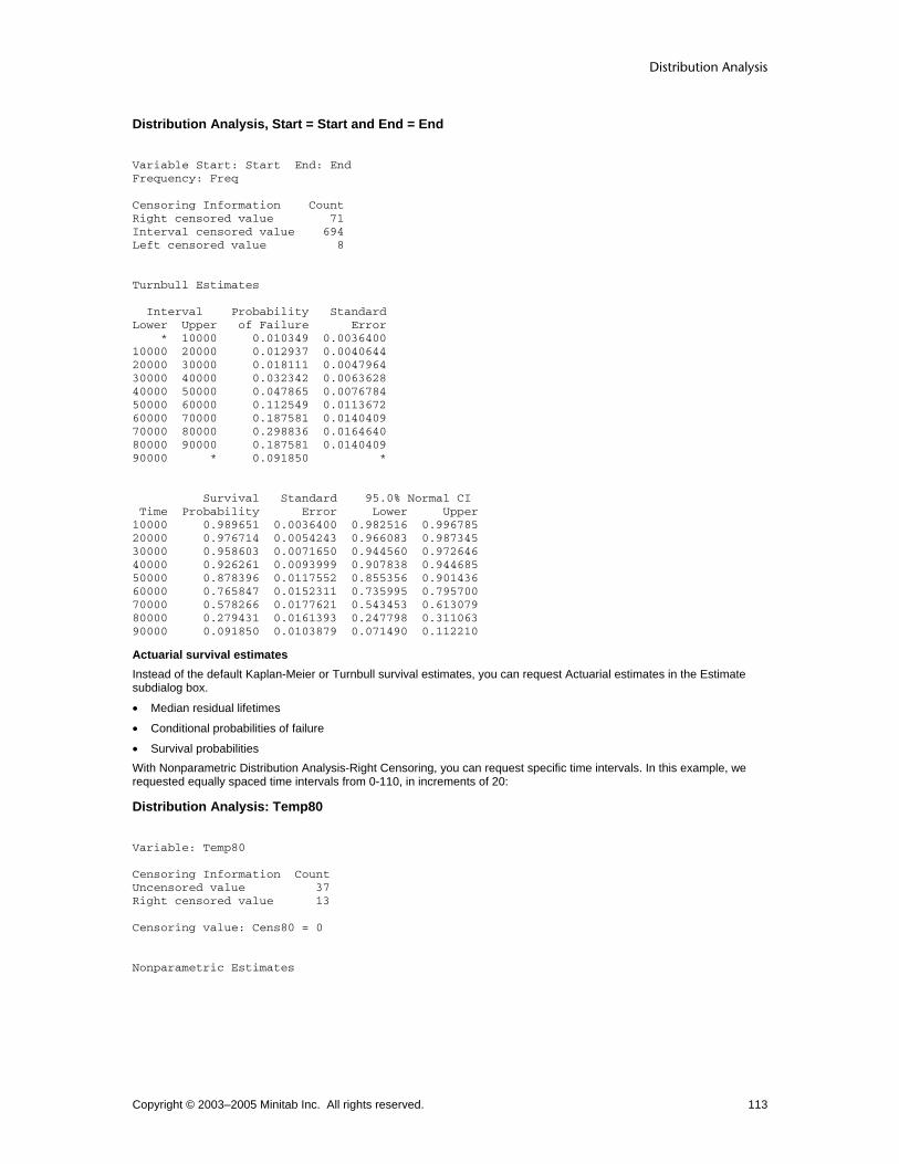
Distribution Analysis
Copyright © 2003–2005 Minitab Inc. All rights reserved. 113
Distribution Analysis, Start = Start and End = End Variable Start: Start End: End Frequency: Freq Censoring Information Count Right censored value 71 Interval censored value 694 Left censored value 8 Turnbull Estimates Interval Probability Standard Lower Upper of Failure Error * 10000 0.010349 0.0036400 10000 20000 0.012937 0.0040644 20000 30000 0.018111 0.0047964 30000 40000 0.032342 0.0063628 40000 50000 0.047865 0.0076784 50000 60000 0.112549 0.0113672 60000 70000 0.187581 0.0140409 70000 80000 0.298836 0.0164640 80000 90000 0.187581 0.0140409 90000 * 0.091850 * Survival Standard 95.0% Normal CI Time Probability Error Lower Upper10000 0.989651 0.0036400 0.982516 0.99678520000 0.976714 0.0054243 0.966083 0.98734530000 0.958603 0.0071650 0.944560 0.97264640000 0.926261 0.0093999 0.907838 0.94468550000 0.878396 0.0117552 0.855356 0.90143660000 0.765847 0.0152311 0.735995 0.79570070000 0.578266 0.0177621 0.543453 0.61307980000 0.279431 0.0161393 0.247798 0.31106390000 0.091850 0.0103879 0.071490 0.112210
Actuarial survival estimates Instead of the default Kaplan-Meier or Turnbull survival estimates, you can request Actuarial estimates in the Estimate subdialog box.
• Median residual lifetimes
• Conditional probabilities of failure
• Survival probabilities With Nonparametric Distribution Analysis-Right Censoring, you can request specific time intervals. In this example, we requested equally spaced time intervals from 0-110, in increments of 20:
Distribution Analysis: Temp80 Variable: Temp80 Censoring Information Count Uncensored value 37 Right censored value 13 Censoring value: Cens80 = 0 Nonparametric Estimates
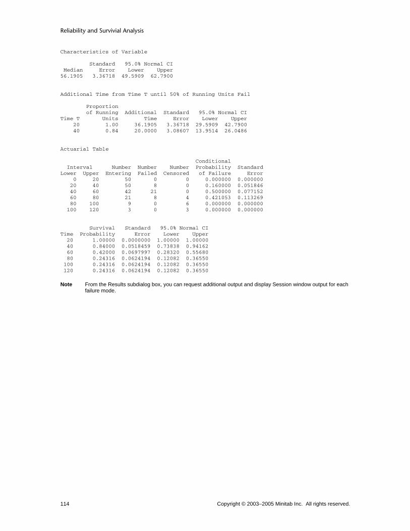
Reliability and Survivial Analysis
Copyright © 2003–2005 Minitab Inc. All rights reserved. 114
Characteristics of Variable Standard 95.0% Normal CI Median Error Lower Upper 56.1905 3.36718 49.5909 62.7900 Additional Time from Time T until 50% of Running Units Fail Proportion of Running Additional Standard 95.0% Normal CI Time T Units Time Error Lower Upper 20 1.00 36.1905 3.36718 29.5909 42.7900 40 0.84 20.0000 3.08607 13.9514 26.0486 Actuarial Table Conditional Interval Number Number Number Probability StandardLower Upper Entering Failed Censored of Failure Error 0 20 50 0 0 0.000000 0.000000 20 40 50 8 0 0.160000 0.051846 40 60 42 21 0 0.500000 0.077152 60 80 21 8 4 0.421053 0.113269 80 100 9 0 6 0.000000 0.000000 100 120 3 0 3 0.000000 0.000000 Survival Standard 95.0% Normal CI Time Probability Error Lower Upper 20 1.00000 0.0000000 1.00000 1.00000 40 0.84000 0.0518459 0.73838 0.94162 60 0.42000 0.0697997 0.28320 0.55680 80 0.24316 0.0624194 0.12082 0.36550 100 0.24316 0.0624194 0.12082 0.36550 120 0.24316 0.0624194 0.12082 0.36550
Note From the Results subdialog box, you can request additional output and display Session window output for each failure mode.

Growth Curves
Copyright © 2003–2005 Minitab Inc. All rights reserved. 115
Growth Curves Growth Curve Overview Use growth curves to analyze life data from a repairable system. A repairable system is one in which the parts are repaired instead of being replaced when they fail. For example, automotive engines are usually repaired many times before being replaced. System repair data usually consist of successive failure (or repair) times. However, data can also be measures such as distance from a reference point or the length of a crack.
• Use nonparametric growth curves to estimate growth curves of the mean cost of maintaining the system or the mean number of repairs over time without making assumptions about the distribution of the cost or number of repairs.
• Use parametric growth curves to estimate growth curves of the mean number of repairs and ROCOF over time using a power-law process or a homogeneous Poisson process.
Use nonparametric and parametric growth curves to determine whether a trend exists in times between successive failures of a repairable system; that is, to determine whether system failures are becoming more frequent, less frequent, or remaining constant. Use this information to make decisions concerning the future operation of your system, such as:
• Setting maintenance schedules
• Making provisions for spare parts
• Assuring suitable performance
• Forecasting repair costs
Data - Growth Curves The data you gather for parametric and nonparametric growth curves are the failure times for a repairable system. For example, an automobile breaks down, is repaired and put back into service, then breaks down again, etc. The data points represent the time of each failure without taking into account the repair time. In other words, the analysis is done as if the system instantaneously works again after failing. This table describes the types of observations you can have.
Type of observation Description Example Exact data You know exactly when each
failure occurred The engine failed at exactly 500 days, was repaired, then failed at 825 days
Interval data You only know that each failure occurred between two particular times
The engine failed sometime between 475 and 500 days, was repaired, and then failed again sometime between 675 and 725 days
How you set up your worksheet depends, in part, on the type of data you have:
• When your data consist of exact failure times, see Growth curves − exact data.
• When your data consist of failures within intervals and you are using nonparametric growth curves, see Growth curves − interval data or Growth curves − grouped interval data.
• When your data consist of failures within intervals and you are using parametric growth curves, see Growth curves − interval data.
Note Stack the system failure time data together if you believe that the rate of failures are identical, as in the case of identical manufacturing processes. Remember to include a system column in this case.
Growth curves - exact data To use growth curves with exact data, you may enter the following information:
• Time − the failure or retirement time of each sample.
• System − identifies each system within a sample. You do not need a system column when you have only one system.
• Retirement − indicates whether the data in each corresponding row is a failure time or a retirement time. Typically, the column will contain two distinct values; one representing failure times, one representing retirement times. By default, the lower value indicates the retirement time for a system. A retirement column is not necessary if all of your data are failure truncated or time truncated.
• Frequency (or Cost) − the total cost of repairs or total frequency of failures at a particular time. You cannot use a cost column with Parametric Growth Curve. See Using cost or frequency columns for more information.

Reliability and Survivial Analysis
Copyright © 2003–2005 Minitab Inc. All rights reserved. 116
This data set illustrates exact data.
Time System Retirement Frequency (or Cost)
1 1 1 2
5 1 1 4
9 1 0 0
4 2 1 2
7 2 1 4
10 2 0 0
8 3 1 2
9 3 1 4
11 3 0 0
Note Retirement times must have a value of 0 in the corresponding frequency column.
Repairable systems data can consist of:
• Failure truncated data: Enter a column of failure times. The retirement time is the largest failure time. A failure-truncated system is retired once a certain number of failures occur. In a failure-truncated system, the system is retired immediately upon the last failure. If the systems in the example above are failure-truncated, system 1 was retired following the failure at 9 hours.
• Time truncated data: Enter a column of failure times. The retirement time for a system is the largest value in the variables (or time) column for that system. A time-truncated system is retired after a specified period of time. In a time-truncated system, the largest time is not a failure time. If the systems in the example above are time-truncated and no retirement column is given, system 1 was retired at 9 hours.
• Data with a retirement column: Enter a column of retirement indicators. Retirement indicators can be numeric, text, or date/time. If you do not specify which value indicates the retirement value in the Retirement subdialog box, Minitab assumes the lower of the two values indicates the retirement value, while the higher one indicates a failure/repair time. If specified, the retirement value applies to every sample in each analysis. The columns for each sample must be the same length, although pairs of columns from different samples can have different lengths. Use retirement columns if one group is time-truncated and another is failure-truncated. In the example above, system 1 failed at the first and fifth hour and is retired at the ninth hour. See Using time and retirement columns for more information about the relationship between your time column and retirement times.
When you have more than one sample, you can use separate columns for each sample. Alternatively, you can stack all the samples in one column, then set up a column of grouping indicators. For an illustration, see Stacked vs. Unstacked data. Each sample is analyzed independently and results in one growth curve. All the samples display on a single plot, with different colors and symbols to help you compare reliability growth between samples.
For general information on repairable systems data, see Data − Growth Curves.
Growth curves - interval data Use a paired response of start and end times when your data are interval failure/retirement times. Enter your data in table form, using Start and End columns:
• Start − the time at the start of the interval.
• End − the time at the end of the interval.
• System − identifies each system within a sample. You do not need a system column when you have only one system.
• Frequency (or Cost) − the total cost of repairs or total frequency of failures at a particular time. See Using cost or frequency columns for more information.

Growth Curves
Copyright © 2003–2005 Minitab Inc. All rights reserved. 117
This data set illustrates interval data, as well as the use of a frequency column.
Start End System Frequency (or Cost)
0 1 1 2
1 5 1 4
9 * 1 0
0 4 2 2
5 7 2 4
10 * 2 0
8 9 3 4
5 8 3 2
11 * 3 0
In this example,
• Two failures occurred between 0 and 1 hours for system 1
• Observation ceased on system 1 at 9 hours When you have more than one sample, you can use separate columns for each sample. Alternatively, you can stack all the samples in one column, then set up a column of grouping indicators. For an illustration, see Stacked vs. Unstacked data. Each sample is analyzed independently and results in one growth curve. All the samples display on a single plot, with different colors and symbols to help you compare reliability growth between samples.
For general information on repairable systems data, see Data − Growth Curves.
Growth curves - grouped interval data Grouped interval data works like interval data except that, instead of a system column, you have a column containing the number of systems. Enter your data in table form, using Start and End columns:
• Start − the time at the start of the interval.
• End − the time at the end of the interval.
• NSystems − the number of systems running at the beginning of each interval.
• Cost − the total cost of repairs in a particular interval.
Note You must have intervals that do not overlap.
This data set illustrates tabled data with a cost column.
Start End NSystems Cost/Total NRepairs
0 5 10 8
5 10 8 10
10 15 6 6
15 * 4 0
In this example,
• Ten systems are running at 0 hours. Between 0 and 5 hours of operation, 8 repairs were made to these systems.
• Four systems are left running after the final observation time of 15 hours. When you have more than one sample, you can use separate columns for each sample. Alternatively, you can stack all the samples in one column, then set up a column of grouping indicators. For an illustration, see Stacked vs. Unstacked data.

Reliability and Survivial Analysis
Copyright © 2003–2005 Minitab Inc. All rights reserved. 118
Each sample is analyzed independently and results in one growth curve. All the samples display on a single plot, with different colors and lines to help you compare reliability growth between samples.
For general information on repairable systems data, see Data − Growth Curves.
Using Cost or Frequency Columns In a parametric analysis, the frequency column represents the total frequency of failures (or number of repairs) at the time listed in the time column.
• If data are exact, it is not theoretically possible to have multiple failures at any one instant for a given system. However, you may need a frequency column because of rounding error that occurred during data collection.
• With interval data, the frequency column indicates the number of failures that have occurred within the corresponding intervals.
In a nonparametric analysis, you can use the column representing the cost/total number of repairs in different ways:
• Total frequency of failures (or number of repairs) at the time listed in the time column
• Cost of each repair
Note If you do not provide a cost or frequency column, Minitab assumes a cost or frequency of 1 for all failures.
Using Time and Retirement Columns The relationship between the time column and the retirement column is summarized below.
• If you provide a retirement column, this column determines whether the time is a failure or a retirement time. Each system must have a retirement time.
• If you do not provide a retirement column and you have only failure-truncated systems, then the retirement time for each system is the largest time for that system. These times are failure times.
• If you have a time-truncated system, then the largest time for each system is the retirement time. This time is not a failure time for that system.
• If you provide multiple retirement columns, and at least one of those columns corresponds to systems that are only time truncated, then you must specify the retirement value. The retirement value will apply to every retirement column.
Parametric Growth Curve Parametric Growth Curve Stat > Reliability/Survival > Parametric Growth Curve Use to perform a parametric analysis on a repairable system. Use either a power-law process or a homogeneous Poisson process to estimate the mean number of failures or the ROCOF over time. If you have a column of data from more than one system, Minitab assumes that your data are from identical processes and provides a pooled growth curve estimate. In this case, Minitab tests for equal shapes or scales across these systems. See Test for equal shapes or scales. If you provide a By variable or two or more columns (exact data) or pairs of columns (interval data), Minitab will also compare across growth curves modeling the different processes. See Test for equal shapes or scales across growth curves.
Dialog box items Data are exact failure/retirement times Choose if you have exact data. Data are interval failure/retirement times Choose if you have interval data.
Variables/Start variables: Enter columns (one column per sample) containing the start times. End variables: If you have interval repair times, enter columns (one column per sample) of end times.
Freq. columns (optional): Enter columns (one column per sample) of frequency data. The columns must contain positive integers (exact data) or nonnegative integers (interval data). System ID (optional): Enter columns (one column per sample) to identify the systems. If a single response column represents more than one system, you must use a System ID column. This results in an additional test for equal shape parameters. By variable: Check if all of the samples are stacked into one column and enter a column of grouping indicators.

Growth Curves
Copyright © 2003–2005 Minitab Inc. All rights reserved. 119
To use parametric growth curves when data are exact failure/retirement times 1 Choose Stat > Reliability/Survival > Parametric Growth Curve. 2 In Variables/Start variables, enter the column containing the failure/retirement times. 3 If your data are from more than one system, choose System ID and enter one column for each sample to identify the
systems within the sample. 4 If you like, use any dialog box options, then click OK.
To use parametric growth curves when data are interval failure/retirement times 1 Choose Stat > Reliability/Survival > Parametric Growth Curve. 2 Choose Data are interval (failure/retirement) times. 3 In Variables/Start variables, enter the column containing the start time of each failure interval. 4 In End variables, enter the column containing the corresponding end time of each failure interval. You must have the
same number of end variable columns as you have start variable columns. 5 If your data are from more than one system, choose System ID and enter one column for each sample to identify the
systems within the sample. 6 If you like, use any dialog box options, then click OK.
Parametric Growth Curve Models The first step in the analysis of a repairable system is to check for a trend in the rate of failures or repairs. Minitab provides two types of models for estimating parametric growth curves:
• Power-law process − Use to model failure/repair times that have an increasing, decreasing, or constant rate. The repair rate for a power-law process is a function of time. With the default (maximum likelihood) estimation method, the power-law model is also referred to as the AMSAA model. With the least squares estimation method, the power-law model is also known as the Duane model.
• Poisson process − Use to model failure/repair times that remain stable over time. Choose your model based on whether or not a trend exists in the failure/repair rate.
Test for Equal Shapes or Scales When your failure/repair data are from more than one system, Minitab provides:
• A test for equal shapes − if you do not provide a known shape • A for equality of the scale parameter − if you provide a known shape • A test for equal MTBFs − if the shape is set at 1
Each of these tests uses the Bartlett's modified likelihood ratio test whenever possible. The hypotheses for these tests are:
• H0: all of the shapes (or scales or MTBFs) are equal
• H1: at least one of the shapes (or scales or MTBFs) is different When estimating a parametric growth curve, Minitab assumes that all systems within a single data column are from identical processes. If you reject the null hypothesis and conclude that the shapes (or scales or MTBFs) are unequal, you cannot make this assumption. In this case, you should analyze the data from different systems separately.
Note These tests are not available for interval data.
Test for Equal Shapes or Scales Across Growth Curves When your failure/repair data are from more than one growth curve, Minitab first performs an analysis on each growth curve. Then it uses the resulting estimates to provide a likelihood ratio test for:
• Equal shapes across groups − if you do not provide a known shape
• Equal scales across groups − if you provide a known shape
• Equal MTBFs across groups − if the shape is set at 1 The hypotheses for these tests are:
• H0: all of the shapes (or scales or MTBFs) are equal

Reliability and Survivial Analysis
Copyright © 2003–2005 Minitab Inc. All rights reserved. 120
• H1: at least one of the shapes (or scales or MTBFs) is different
Note These tests are not available for interval data.
Trend tests The tests for trend are sometimes referred to as goodness of fit tests. Use the tests for trend to determine whether a homogeneous Poisson process or a nonhomogeneous Poisson process is the appropriate model. Regardless of the model you choose, the hypotheses for the tests for trend test are generally: H0: No trend in data (homogeneous Poisson process) H1:Trend in data (nonhomogeneous Poisson process)
• If you reject the null hypothesis, you can conclude that there is some trend in your data and you should model your data with a nonhomogeneous Poisson process such as the power-law process.
• If you fail to reject the null hypothesis, there is insufficient evidence to reject the homogeneous Poisson process model. Although the power-law process may still be appropriate, the homogeneous Poisson process is a simpler model and therefore a better choice.
Note The null hypothesis differs slightly depending on which test you are using. See Comparisons of trend tests for more information about which test is most relevant for your data.
With exact data, Minitab provides three trend tests:
• MIL-Hdbk-189 (The military handbook test)
• Laplace
• Anderson-Darling With exact data from multiple systems, Minitab provides five trend tests:
• MIL-Hdbk-189 (pooled)
• MIL-Hdbk-189 (TTT-based)
• Laplace (pooled)
• Laplace (TTT-based)
• Anderson-Darling With interval data, Minitab provides only the MIL-Hdbk-189 test.
Note Simulation studies have shown that a fairly large difference in p-values between TTT-based tests (including the Anderson-Darling test) and the pooled tests may indicate heterogeneity between systems. You may need to analyze the data separately for each system.
Comparison of trend tests Minitab provides five trend tests for data with multiple systems: MIL-hdbk-189 (TTT-based), MIL-hdbk-189 (Pooled), Laplace's (TTT-based), Laplace's (Pooled), and Anderson-Darling. The pooled Laplace and military handbook tests reduce to their respective TTT-based tests when there is only one system. These tests behave differently under the following two circumstances: 1 the data follow a non-monotonic trend 2 the data are from heterogeneous systems
Monotonic and non-monotonic trends There is a trend in the pattern of times between failure if the times change in a systematic way. Trends can be:
• monotonic − times between failures are getting either consistently longer (decreasing trend) or consistently shorter (increasing trend)
• non-monotonic − times between failures alternate between increasing and decreasing trend (cyclic) or have a decreasing trend, no trend, and then increasing trend (bathtub)
The Anderson-Darling test will reject the null hypothesis in the presence of both monotonic and non-monotonic trends. The other tests will generally only detect monotonic trends. While the Anderson-Darling test is useful if you suspect the existence of a cyclic or other non-monotonic trend, the other tests are more powerful in the case of a monotonic trend.
Homogeneous and heterogeneous systems The null hypothesis of no trend differs slightly for the different tests:
• The null hypothesis for the pooled tests (MIL-hdbk-189 and Laplace's) is that the data come from a homogeneous Poisson processes (HPP) with a possibly different MTBF for each system. Thus, rejecting the null hypothesis means that you can definitely conclude there is a trend in your data.

Growth Curves
Copyright © 2003–2005 Minitab Inc. All rights reserved. 121
• The null hypothesis for the TTT-based tests (MIL-hdbk-189, Laplace's, and Anderson-Darling) is that the data come from a homogeneous Posson process (HPP) with the same MTBF for each system. Thus, rejecting the null hypothesis could mean that either there is a trend in your data or your data come from heterogeneous systems. Therefore, you should use TTT-based tests only when you are confident that your systems are homogeneous.
The table below summarizes the different null hypotheses associated with the trend tests.
MIL-hdbk-189 (Pooled)
MIL-hdbk-189 (TTT-based)
Laplace's (Pooled)
Laplace's (TTT-based)
Anderson-Darling
Null Hypothesis
HPP (possibly different MTBFs)
HPP (equal MTBFs)
HPP (possibly different MTBFs)
HPP (equal MTBFs)
HPP (possibly different MTBFs)
Rejecting H0 means...
monotonic trend monotonic trend or systems are heterogeneous
monotonic trend monotonic trend or systems are heterogeneous
monotonic trend or non-monotonic trend or systems are heterogeneous
See [12] for more information concerning these tests.
Using Parametric Growth Curve to find the probability of failure You can use the results from Parametric Growth Curve to estimate the probability of failure within a given time frame.
The estimated mean cumulative function ( ) = where
• t = the time since the start of the test
• = the estimated shape parameter
• = the estimated scale parameter The probability that at least one failure will occur between now (t) and the next t1 days is:
where X is the number of failures in the time interval (t, t+t1]. For example, assume you are analyzing machinery breakdown and want to find the probability of at least one breakdown in the next seven days. You use Parametric Growth Curve to estimate the current value of the MCF and obtain the following estimates of shape and scale respectively:
• = 0.5
• = 3.5 If the test has already been running for t = 8 days, the probability of at least one failure in the next 7 days is:
Parametric Growth Curve − Retirement Stat > Reliability/Survival > Parametric Growth Curve > Retirement Use to specify the retirement information.
Dialog box items Retirement time at largest time for system Choose if the largest time for each system is the retirement time for the system.
Failure truncated systems: Choose if you have failure-truncated data only; that is, the system is retired immediately upon the last failure. Time truncated systems: Choose if you have time-truncated data only; that is, the largest time for each system is not a failure time.
Retirement time defined by retirement columns Choose to define the retirement time when you have both failure-truncated and time-truncated systems. See Using time and retirement columns for more information.
Retirement columns: Enter the retirement columns in the box. The first retirement column is paired with the first data column, the second retirement column is paired with the second data column, and so on. All retirement columns must have exactly two distinct values unless you specify a retirement value.

Reliability and Survivial Analysis
Copyright © 2003–2005 Minitab Inc. All rights reserved. 122
Retirement value: Enter a value indicating which value in your retirement column represents a retired system. If you do not enter a value, the lowest value in the retirement column is the retirement value. Text values must be contained in double quotes.
Note You cannot use a retirement column when you have interval data.
Parametric Growth Curve − Estimate Stat > Reliability/Survival > Parametric Growth Curve > Estimate Use to specify one of three estimation methods and either a power-law process or Poisson process model. You can also enter a confidence level for Minitab to use for all confidence intervals.
Dialog box items Estimation method: Choose one of three estimation methods: maximum likelihood, conditional maximum likelihood, and least squares. See Estimation methods for parametric growth curves. Power-Law process Choose to model the data using a Power-Law process. See Parametric growth curve models.
Estimate shape parameter: Choose to estimate the shape parameter from the data. Set shape parameter: Choose to specify the shape value and enter a positive numeric constant.
Poisson process: Choose to model the data using a Poisson process. See Parametric growth curve models. Confidence level: Enter a confidence level for all of the confidence intervals. The default is 95.0%. Confidence intervals: Choose to use two-sided confidence intervals (the default) or just an upper or lower confidence bound.
Estimation methods for parametric growth curves Minitab estimates the shape and scale using one of three estimation methods: maximum likelihood, conditional maximum likelihood, and least squares. The log-likelihood is a measure of the fit of the distribution. When estimating the shape and scale parameters, Minitab will make this number as large as possible. By maximizing the likelihood function, Minitab calculates the maximum likelihood and conditional maximum likelihood estimates. Minitab displays output in the Session window based on the chosen estimation method and whether or not the shape parameter is known. The differences are shown in the table below:
Method Shape Parameter estimates Standard error and confidence intervals
Maximum likelihood Unknown Shape and scale Yes Maximum likelihood Known, = 1 MTBF Yes Maximum likelihood Known, not 1 Scale Yes Conditional maximum likelihood Unknown Shape and scale For shape only Least squares Unknown Shape and scale No Least squares Known, = 1 MTBF No Least squares Known, not 1 Scale No
See Comparison of growth curve procedures for a discussion of the advantages and disadvantages of each method.
Comparison of growth curve procedures Minitab provides three estimation methods for the parameter estimates: maximum likelihood, conditional maximum likelihood, and least squares. The table below summarizes the features available with each estimation method.
MLE CMLE LSYXExact standard error and confidence interval for the shape No Yes No Asymptotic standard error and confidence interval for the shape Yes No No Asymptotic standard error and confidence interval for the scale Yes No No Non-iterative solutions, even when data are from multiple systems No Yes Yes Comparison of estimates between growth curves Yes Yes No Available for interval data Yes No Yes Available when the shape is specified Yes No Yes

Growth Curves
Copyright © 2003–2005 Minitab Inc. All rights reserved. 123
Parametric Growth Curve − Graphs Stat > Reliability/Survival > Parametric Growth Curve > Graphs Use to create an event plot, mean cumulative function and Nelson-Aalen plot, Duane plot, or total-time-on-test plot.
Dialog box items Event Plot Check to display an event plot.
Display number of failures on event plot: Check to display the frequency of failures on the event plot. Mean cumulative function (MCF) and Nelson-Aalen plot: Check to display the estimated mean cumulative function overlaid on the Nelson-Aalen plot.
Display confidence intervals on MCF plot: Check to display confidence intervals on the MCF plot. By default, Minitab plots a 95% confidence interval. You can change the confidence level in the Estimate subdialog box.
Duane plot: Check to display a Duane plot. Total time on test (TTT) plot Check to display a total-time-on-test plot. Display (except event plot):
An average plot over all systems: Choose to create plots which are averaged over (or pooled across) all systems. This option does not apply to the event plot. One plot per system: Choose to create separate plots for each system. This option does not apply to the event plot.
Show graphs of different variables/by levels or systems: Choose to display the graphs overlaid on the same page or on separate pages. X axis display (except TTT plot): Minimum X scale: Enter a value for the minimum x-axis scale. This option does not apply to the TTT plot. Maximum X scale: Enter a value for the maximum x-axis scale. This option does not apply to the TTT plot. X axis label: Type the desired text to replace the default x-axis label with your own label. This option does not apply to the TTT plot.
Mean Cumulative Function and Nelson-Aalen Plot Use the mean cumulative function and Nelson − Aalen plot to determine whether your system is improving, deteriorating, or staying constant. The plot consists of:
• The Nelson-Aalen plot, which is a plot of the empirical mean cumulative function. The plot points do not assume a particular model. When you have interval data, Minitab estimates failure times by evenly distributing the number of occurrences in each interval and plotting the appropriate points.
• The mean cumulative function plot, which is a plot of the mean cumulative function based on the estimated shape and scale. For a power-law process, the rate of system failures can increase, decrease, or remain constant. The resulting graph can be straight or a curve that is either concave up or down. For a homogeneous Poisson process, the failure rate is constant, resulting in a straight line.
Because the Nelson-Aalen plot does not depend on the model, the plot points are the same regardless of which estimation method and model type you chose. The mean cumulative function plot, however, differs depending on your model. The plot provides information about the pattern of system failures:
• A straight line pattern indicates that system failures are remaining constant over time − your system is stable
• A concave down pattern indicates that the time between failures is increasing over time − your system reliability is improving
• A concave up pattern indicates that the time between failures is decreasing over time − your system reliability is deteriorating
Below are examples of mean cumulative function plots for improving, stable, and deteriorating systems.

Reliability and Survivial Analysis
Copyright © 2003–2005 Minitab Inc. All rights reserved. 124
Event plot A plot of events (failures and retirements) for all systems. The plot consists of:
• Horizontal lines, which represent the lifetime of each system
• Cross (X) points, which represent the failure and retirement times of each system
• Cost values or frequencies (optional), which represent the cost or frequency of failure at the cross points Use the event plot to visually determine whether successive failures are increasing, decreasing, or remaining constant. Below are examples of event plots for improving, stable, and deteriorating systems.

Growth Curves
Copyright © 2003–2005 Minitab Inc. All rights reserved. 125
Note For interval data, the event plot is constructed using the midpoint of each interval.
Duane plot A scatterplot of the cumulative number of failures at a particular time divided by the time (cumulative failure rate) versus time. Use a Duane plot to:
• Assess whether your data follow a power-law process or a homogeneous Poisson process
• Determine if your system is improving, deteriorating, or remaining stable The fitted line on the Duane plot is the best fitted line when the assumption of the power-law process is valid and the shape and scale are estimated using the least squares method. See Methods and Formulas for the formula for the fitted line. The Duane plot should be roughly linear if the power-law process or homogeneous Poisson process is appropriate. A negative slope shows reliability improvement, a positive slope shows reliability deterioration, and no slope (a horizontal line) shows a stable system. Below are examples of Duane plots for improving, stable, and deteriorating systems.

Reliability and Survivial Analysis
Copyright © 2003–2005 Minitab Inc. All rights reserved. 126
Total Time on Test Plot Use a total-time-on-test (TTT) plot to visualize how well your model fits the data. The TTT plot provides a graphical goodness-of-fit test for the power-law process.
• A power-law process is appropriate if the TTT plot lies close to the diagonal or is a curve that is either concave up or concave down
• If there is no pattern, or a curve that shifts between being concave up and concave down, the power-law process is inadequate
Below are examples of total time on test plots for improving, stable, and deteriorating systems.

Growth Curves
Copyright © 2003–2005 Minitab Inc. All rights reserved. 127
Parametric Growth Curve − Results Stat > Reliability/Survival > Parametric Growth Curve > Results Use to control the display of the Session window output.
Dialog box items Show log-likelihood for each iteration of algorithm Check to display the value of the shape, scale, and the log-likelihood at each iteration when available.
Parametric Growth Curve − Options Stat > Reliability/Survival > Parametric Growth Curve > Options Use to specify starting estimates for the shape and the maximum number of iterations when available.
Dialog box items Use starting estimate for shape: Enter starting estimates for the shape. You can provide as many starting estimates as there are response columns. If you provide fewer starting estimates than there are response columns, the last shape value listed is used for the remaining variables. Maximum number of iterations: Enter a positive integer to specify the number of iterations. The default number of iterations is 20.
Parametric Growth Curve − Storage Stat > Reliability/Survival > Parametric Growth Curve > Storage Use to store various characteristics of the parametric growth curve.
Dialog box items Enter number of levels in by variable: If all of the samples are stacked in one column, enter the number of levels the column of grouping indicators contains.
Mean cumulative function (MCF): Store the mean cumulative function evaluated at the corresponding time (exact data) or end time (interval data). Confidence limits for MCF: Check to store the confidence limits for the mean cumulative function. By default, Minitab stores the 95% confidence limits. You can change the confidence level in the Estimate subdialog box.

Reliability and Survivial Analysis
Copyright © 2003–2005 Minitab Inc. All rights reserved. 128
Failure rate (ROCOF): Check to store the ROCOF evaluated at the corresponding time (exact data) or end time (interval data). Confidence limits for ROCOF: Check to store the confidence limits for the ROCOF. By default, Minitab stores the 95% confidence limits. You can change the confidence level in the Estimate subdialog box. Parameter estimates: Check to store estimates of the shape and scale. Standard error of estimates: Check to store the standard errors of the shape and scale where available. Confidence limits for parameters: Check to store the confidence limits for the shape and scale. By default, Minitab stores the 95% confidence limits. You can change the confidence level in the Estimate subdialog box.
Example of Parametric Growth Curve You want to estimate the replacement rate of a certain valve on a fleet of 65 diesel engines. 1 Open the worksheet VSEAT.MTW. 2 Choose Stat > Reliability/Survival > Parametric Growth Curve. 3 In Variable/Start variables, enter Days. 4 In System ID, enter ID. 5 Click OK.
Session window output
Parametric Growth Curve: Days System: ID Model: Power-Law Process Estimation Method: Maximum Likelihood Parameter Estimates Standard 95% Normal CI Parameter Estimate Error Lower Upper Shape 4.00405 0.406 3.28239 4.88436 Scale 420.130 18.590 385.229 458.193 Test for Equal Shape Parameters Bartlett's Modified Likelihood Ratio Chi-Square Test Statistic 23.62 P-Value 0.425 DF 23 Trend Tests MIL-Hdbk-189 Laplace's TTT-based Pooled TTT-based Pooled Anderson-DarlingTest Statistic 34.73 33.20 9.13 5.73 50.59P-Value 0.000 0.000 0.000 0.000 0.000DF 142 96

Growth Curves
Copyright © 2003–2005 Minitab Inc. All rights reserved. 129
Graph window output
Interpreting the results The estimate of the shape (4.004) is greater than 1, indicating that the failure rate is increasing. You can be 95% confident that the interval (3.282, 4.884) contains the true shape.

Reliability and Survivial Analysis
Copyright © 2003–2005 Minitab Inc. All rights reserved. 130
The test for equal shape parameters indicates that there is not enough evidence to say that the systems come from populations with different shapes (P-Value = 0.425). The pooled estimate of the shape is valid. The tests for trend are all significant (P-Value = 0.000). This means that there is enough evidence to reject the null hypothesis that there is no trend in your data. You can conclude that the increasing trend is significant. The event plot seems to show a pattern of failures that become more frequent as time goes on. The plot of the MCF versus time shows a curve that is concave up. This plot is consistent with a shape that is greater than one, or a system that is deteriorating.
Nonparametric Growth Curve Nonparametric Growth Curve Stat > Reliability/Survival > Nonparametric Growth Curve Use to perform a nonparametric analysis on a repairable system when you want to estimate a growth curve of the mean cost of maintaining a system or the mean number of repairs over time without assuming a distribution. If you provide two or more columns (exact data) or pairs of columns (interval data), Minitab compares the different repairable systems.
Dialog box items Data are exact failure/retirement times Choose if you have exact data. Data are interval failure/retirement times Choose if you have interval data.
Variables/Start variables: Enter columns (one column per sample) containing the start times. End variables: If you have interval repair times, enter columns (one column per sample) of end times.
System Information If you do not provide any system information, Minitab assumes that all data are from the same system.
System ID: Choose to identify the systems within the sample, then enter one column for each sample. If a single response column represents more than one system, you must use a System ID column. Number of systems: Choose if your data are grouped, then enter one column for each sample to specify the number systems entering each time interval. Your data must be in interval format to use this option.
By variable: Check if all of the samples are stacked in one column and enter a column of grouping indicators.
To use nonparametric growth curves when data are exact (failure/retirement) times 1 Choose Stat > Reliability/Survival > Nonparametric Growth Curve. 2 In Variables/Start variables, enter the column containing the failure/retirement times. 3 If your data are from more than one system, choose System ID and enter one column for each sample to identify the
systems within the sample. 4 If you like, use any dialog box options, then click OK.
To use nonparametric growth curves when data are interval (failure/retirement) times 1 Choose Stat > Reliability/Survival > Nonparametric Growth Curve. 2 Choose Data are interval (failure/retirement) times. 3 In Variables/Start variables, enter the column containing the start time of each failure interval. 4 In End variables, enter the column containing the end time of each failure interval. You must have the same number
of end variable columns as you have start variable columns. 5 If your data are from more than one system, do one of the following:
• Choose System ID and enter one column for each sample to identify the systems within the sample • Choose Number of systems and enter one column for each sample to specify the number of systems entering
each time interval 6 If you like, use any dialog box options, then click OK.

Growth Curves
Copyright © 2003–2005 Minitab Inc. All rights reserved. 131
Nonparametric Growth Curve − Retirement Stat > Reliability/Survival> Nonparametric Growth Curve > Retirement Use to specify the retirement information.
Dialog box items Retirement time at largest time for system Choose if the largest time for each system is the retirement time for the system.
Failure truncated systems: Choose if you have failure-truncated data only; that is, the system is retired immediately upon the last failure. Time truncated systems: Choose if you have time-truncated data only; that is, the largest time for each system is not a failure time.
Retirement time defined by retirement columns Choose to define the retirement time. See Using time and retirement columns for more information.
Retirement columns: Enter the retirement columns in the box. The first retirement column is paired with the first data column, the second retirement column is paired with the second data column, and so on. All retirement columns must have exactly two distinct values unless you specify a retirement value. Retirement value: If you like, enter a value indicating which value in your retirement column represents a retired system. If you do not enter a value, the lowest value in the retirement column is the retirement value. Text values must be contained in double quotes.
Note You cannot use a retirement column when you have interval data.
Nonparametric Growth Curve − Cost-Freq Stat > Reliability/Survival > Nonparametric Growth Curve > Cost-Freq Use to enter the total cost of repairs or number of repairs for each row of data. If you do not provide this column, Minitab assumes a cost of 1 for all failures. You must provide a cost/frequency column if you have grouped interval data.
Dialog box items Repair cost/number of repairs for systems: Enter a column containing the total cost of repairs or total frequency of repairs. The column must contain numeric values greater than or equal to 0. The value in this column must be 0 for a retired system. The first cost column is paired with the first data column, the second cost column is paired with the second data column, and so on.
Nonparametric Growth Curve − Graphs Stat > Reliability/Survival > Nonparametric Growth Curve > Graphs Use to create an event plot, plot of the mean cumulative function, or plot of the mean cumulative difference function.
Dialog box items Event Plot Check to display an event plot.
Display cost/number of repairs on event plot: Check to display the cost or number of repairs on the event plot. Mean cumulative function: Check to display a plot of the mean cumulative function. Mean cumulative difference function: Check to display a plot of the mean cumulative difference function. This plot is only available when you have multiple samples. Display confidence intervals on plots: Check to display confidence intervals on the mean cumulative function and mean cumulative difference function plots. By default, Minitab plots a 95% confidence interval. You can change the confidence level in the Options subdialog box. Confidence intervals are only calculated when you have multiple systems. Show graphs of different variables or by levels: Choose to display the graphs overlaid on the same page or on separate pages. Event plots are always on separate pages. Minimum X scale: Enter a value for the minimum x-axis scale. Maximum X scale: Enter a value for the maximum x-axis scale. X axis label: Type the desired text to replace the default x-axis label with your own label.
Event plot A plot of events (failures and retirements) for all systems. The plot consists of:
• Horizontal lines, which represent the lifetime of each system

Reliability and Survivial Analysis
Copyright © 2003–2005 Minitab Inc. All rights reserved. 132
• Cross (X) points, which represent the failure and retirement times of each system
• Cost values or frequencies (optional), which represent the cost or frequency of failure at the cross points Use the event plot to visually determine whether successive failures are increasing, decreasing, or remaining constant. Below are examples of event plots for improving, stable, and deteriorating systems.
Note For interval data, the event plot is constructed using the midpoint of each interval.
Mean Cumulative Function Plot Use the mean cumulative function plot to visualize whether your system reliability is improving, deteriorating, or staying constant. The mean cumulative function plot displays the mean cumulative function versus time. The plot is a step function with steps at system failures or endpoints of intervals. When you have interval data, Minitab plots the middle point. The plot provides information about the pattern of system failures:
• A straight line indicates that system failures are remaining constant over time
• A curve that is concave down indicates that the time between failures is increasing over time − your system reliability is improving
• A curve that is concave up indicates that the time between failures is decreasing over time − your system reliability is deteriorating
Below are examples of mean cumulative function plots for improving, stable, and deteriorating systems.
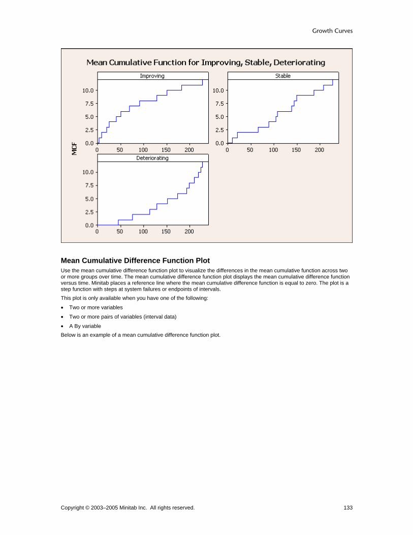
Growth Curves
Copyright © 2003–2005 Minitab Inc. All rights reserved. 133
Mean Cumulative Difference Function Plot Use the mean cumulative difference function plot to visualize the differences in the mean cumulative function across two or more groups over time. The mean cumulative difference function plot displays the mean cumulative difference function versus time. Minitab places a reference line where the mean cumulative difference function is equal to zero. The plot is a step function with steps at system failures or endpoints of intervals. This plot is only available when you have one of the following:
• Two or more variables
• Two or more pairs of variables (interval data)
• A By variable Below is an example of a mean cumulative difference function plot.

Reliability and Survivial Analysis
Copyright © 2003–2005 Minitab Inc. All rights reserved. 134
Nonparametric Growth Curve − Options Stat > Reliability/Survival > Nonparametric Growth Curve > Options Use to specify the confidence level and type of confidence interval.
Dialog box items Confidence level: Enter a confidence level for all of the confidence intervals. The default is 95.0%. Confidence intervals: Choose to use two-sided confidence intervals (the default) or just an upper or lower confidence bound.
Nonparametric Growth Curve − Storage Stat > Reliability/Survival > Nonparametric Growth Curve > Storage Use to store various characteristics of the nonparametric growth curve.
Dialog box items Enter number of levels in by variable: Enter the number of levels the column of grouping indicators contains. Use only if all of the samples are stacked in one column. Individual curve
Mean cumulative function (MCF): Check to store the mean cumulative function. Times for MCF: Check to store the times associated with the mean cumulative function. Standard error of MCF: Check to store the standard error of the mean cumulative function. Confidence limits for MCF: Check to store the confidence limits for the mean cumulative function. By default, Minitab stores the 95% confidence limits. You can change the confidence level in the Options subdialog box.
Difference in individual Difference in mean cumulative function (MCF): Check to store the mean cumulative difference function. Times for difference in MCF: Check to store the times associated with the mean cumulative difference function. Standard error of difference in MCF: Check to store the standard error of the mean cumulative difference function.

Growth Curves
Copyright © 2003–2005 Minitab Inc. All rights reserved. 135
Confidence limits for difference in MCF: Check to store the confidence limits for the mean cumulative difference function. By default, Minitab stores the 95% confidence limits. You can change the confidence level in the Options subdialog box.
Example of Nonparametric Growth Curve You want to compare two different types of a particular brake component used on a subway train. Your data include replacement times and component type for 29 trains. The final time for each train is the final failure for that train. 1 Open the worksheet TRAIN.MTW. 2 Choose Stat > Reliability/Survival > Nonparametric Growth Curve. 3 In Variables/Start variables, enter Days. 4 Under System Information, choose System ID, then enter ID. 5 Check By variable, then enter Type. 6 Click OK.
Session window output
Nonparametric Growth Curve: Days Results for Type = 1 System: ID Nonparametric Estimates Table of Mean Cumulative Function Mean Cumulative Standard 95% Normal CI Time Function Error Lower Upper System 33 0.07143 0.068830 0.01081 0.47218 179 88 0.14286 0.093522 0.03960 0.51540 132 250 0.21429 0.109664 0.07859 0.58426 128 272 0.28571 0.120736 0.12481 0.65408 137 287 0.35714 0.128060 0.17686 0.72120 181 302 0.42857 0.132260 0.23407 0.78471 119 317 0.50000 0.133631 0.29613 0.84423 182 364 0.57143 0.132260 0.36303 0.89945 112 367 0.64286 0.128060 0.43506 0.94990 167 391 0.71429 0.157421 0.46374 1.10019 112 402 0.78571 0.149098 0.54168 1.13970 175 421 0.85714 0.170747 0.58008 1.26653 137 431 0.92857 0.158574 0.66444 1.29771 155 444 1.00000 0.174964 0.70969 1.40906 119 462 1.07143 0.158574 0.80165 1.43200 101 481 1.14286 0.137661 0.90253 1.44718 145 498 1.21429 0.149098 0.95456 1.54468 182 500 1.28571 0.187044 0.96675 1.70992 119 500 1.35714 0.191853 1.02872 1.79042 128 548 1.42857 0.219328 1.05735 1.93013 112 552 1.50000 0.242226 1.09304 2.05848 137 625 1.57143 0.280566 1.10744 2.22982 137 635 1.64286 0.259653 1.20522 2.23940 169 650 1.71429 0.256120 1.27912 2.29750 169 657 1.78571 0.270649 1.32679 2.40338 182 687 1.86264 0.266655 1.40692 2.46596 179 687 1.93956 0.260862 1.49012 2.52456 181 700 2.03047 0.254826 1.58771 2.59671 175 708 2.13047 0.274527 1.65498 2.74258 169 710 2.24158 0.268755 1.77214 2.83537 145 710 2.35269 0.257586 1.89833 2.91581 155 710 2.46380 0.240267 2.03516 2.98273 167 719 2.63047 0.347216 2.03084 3.40714 137 724 2.83047 0.425594 2.10800 3.80055 112 724 3.03047 0.443994 2.27405 4.03849 128 724 3.23047 0.410559 2.51818 4.14424 132

Reliability and Survivial Analysis
Copyright © 2003–2005 Minitab Inc. All rights reserved. 136
730 3.73047 0.471307 2.91221 4.77864 101 730 4.23047 0.410559 3.49769 5.11677 119 Results for Type = 2 System: ID Nonparametric Estimates Table of Mean Cumulative Function Mean Cumulative Standard 95% Normal CI Time Function Error Lower Upper System 19 0.06667 0.064406 0.01004 0.44284 228 22 0.13333 0.087771 0.03670 0.48447 212 39 0.20000 0.103280 0.07269 0.55029 192 54 0.26667 0.114180 0.11521 0.61721 214 61 0.33333 0.121716 0.16295 0.68186 219 91 0.40000 0.157762 0.18465 0.86652 192 93 0.46667 0.159629 0.23869 0.91237 243 119 0.53333 0.207989 0.24834 1.14538 192 148 0.60000 0.263312 0.25386 1.41809 192 173 0.66667 0.261052 0.30945 1.43622 190 185 0.73333 0.274334 0.35227 1.52661 228 187 0.80000 0.269979 0.41289 1.55006 235 192 0.86667 0.264435 0.47658 1.57604 205 194 0.93333 0.257624 0.54335 1.60321 216 203 1.00000 0.249444 0.61330 1.63052 183 205 1.06667 0.257624 0.66442 1.71243 243 211 1.13333 0.264435 0.71738 1.79046 183 242 1.20000 0.269979 0.77210 1.86504 190 250 1.26667 0.257624 0.85023 1.88706 204 264 1.33333 0.277555 0.88664 2.00507 243 277 1.40000 0.295146 0.92615 2.11630 183 293 1.46667 0.280740 1.00786 2.13434 184 306 1.53333 0.324779 1.01238 2.32237 192 369 1.60000 0.309839 1.09468 2.33859 206 373 1.66667 0.335548 1.12325 2.47298 183 382 1.73333 0.319258 1.20810 2.48693 200 415 1.80000 0.342540 1.23962 2.61370 243 416 1.87143 0.340512 1.31007 2.67333 235 419 1.94835 0.338097 1.38662 2.73764 219 419 2.02527 0.349310 1.44435 2.83985 228 432 2.11618 0.347441 1.53391 2.91948 216 434 2.21618 0.345034 1.63337 3.00696 204 441 2.32729 0.341839 1.74512 3.10369 214 447 2.45229 0.337430 1.87262 3.21141 212 448 2.59515 0.331033 2.02109 3.33227 205 448 2.73801 0.315398 2.18466 3.43152 206 460 2.93801 0.298009 2.40832 3.58420 200 461 3.18801 0.449834 2.41776 4.20364 192 464 3.52134 0.511478 2.64893 4.68108 190 503 4.02134 0.535360 3.09778 5.22025 184 511 5.02134 0.535360 4.07443 6.18831 183 Comparisons for Days Comparison: (Type = 1) - (Type = 2)
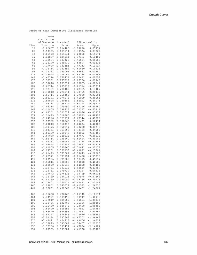
Growth Curves
Copyright © 2003–2005 Minitab Inc. All rights reserved. 137
Table of Mean Cumulative Difference Function Mean Cumulative Difference Standard 95% Normal CI Time Function Error Lower Upper 19 -0.06667 0.064406 -0.19290 0.05957 22 -0.13333 0.087771 -0.30536 0.03869 33 -0.06190 0.111541 -0.28052 0.15671 39 -0.12857 0.124114 -0.37183 0.11469 54 -0.19524 0.133322 -0.45654 0.06607 61 -0.26190 0.139830 -0.53597 0.01216 88 -0.19048 0.153496 -0.49132 0.11037 91 -0.25714 0.183399 -0.61660 0.10231 93 -0.32381 0.185008 -0.68642 0.03880 119 -0.39048 0.228047 -0.83744 0.05649 148 -0.45714 0.279427 -1.00481 0.09052 173 -0.52381 0.277299 -1.06730 0.01969 185 -0.59048 0.289837 -1.15855 -0.02241 187 -0.65714 0.285719 -1.21714 -0.09714 192 -0.72381 0.280486 -1.27355 -0.17407 194 -0.79048 0.274074 -1.32765 -0.25330 203 -0.85714 0.266399 -1.37928 -0.33501 205 -0.92381 0.274074 -1.46099 -0.38663 211 -0.99048 0.280486 -1.54022 -0.44073 242 -1.05714 0.285719 -1.61714 -0.49714 250 -1.05238 0.279994 -1.60116 -0.50360 264 -1.11905 0.298435 -1.70397 -0.53413 272 -1.04762 0.302679 -1.64086 -0.45438 277 -1.11429 0.318886 -1.73929 -0.48928 287 -1.04286 0.321731 -1.67344 -0.41228 293 -1.10952 0.308568 -1.71431 -0.50474 302 -1.03810 0.310335 -1.64634 -0.42985 306 -1.10476 0.350677 -1.79208 -0.41745 317 -1.03333 0.351196 -1.72166 -0.34500 364 -0.96190 0.350677 -1.64922 -0.27459 367 -0.89048 0.349114 -1.57473 -0.20622 369 -0.95714 0.335260 -1.61424 -0.30004 373 -1.02381 0.359155 -1.72774 -0.31988 382 -1.09048 0.343985 -1.76467 -0.41628 391 -1.01905 0.355960 -1.71672 -0.32138 402 -0.94762 0.352358 -1.63823 -0.25701 415 -1.01429 0.373582 -1.74649 -0.28208 416 -1.08571 0.371724 -1.81428 -0.35715 419 -1.23956 0.379800 -1.98395 -0.49517 421 -1.16813 0.388808 -1.93018 -0.40608 431 -1.09670 0.383618 -1.84858 -0.34482 432 -1.18761 0.381917 -1.93616 -0.43907 434 -1.28761 0.379729 -2.03187 -0.54336 441 -1.39872 0.376828 -2.13729 -0.66015 444 -1.32729 0.384013 -2.07995 -0.57464 447 -1.45229 0.380094 -2.19726 -0.70733 448 -1.73801 0.360677 -2.44492 -1.03109 460 -1.93801 0.345574 -2.61532 -1.26070 461 -2.18801 0.482663 -3.13401 -1.24201 462 -2.11658 0.476966 -3.05142 -1.18174 464 -2.44991 0.535496 -3.49947 -1.40036 481 -2.37849 0.529680 -3.41664 -1.34033 498 -2.30706 0.532767 -3.35126 -1.26285 500 -2.16420 0.546276 -3.23488 -1.09352 503 -2.66420 0.568698 -3.77883 -1.54957 511 -3.66420 0.568698 -4.77883 -2.54957 548 -3.59277 0.578546 -4.72670 -2.45884 552 -3.52134 0.587608 -4.67303 -2.36965 625 -3.44991 0.604423 -4.63456 -2.26527 635 -3.37849 0.595004 -4.54467 -2.21230 650 -3.30706 0.593471 -4.47024 -2.14387 657 -3.23563 0.599884 -4.41138 -2.05988

Reliability and Survivial Analysis
Copyright © 2003–2005 Minitab Inc. All rights reserved. 138
687 -3.08178 0.595533 -4.24900 -1.91456 700 -2.99087 0.592914 -4.15296 -1.82878 708 -2.89087 0.601644 -4.07007 -1.71167 710 -2.55754 0.586803 -3.70765 -1.40743 719 -2.39087 0.638098 -3.64152 -1.14022 724 -1.79087 0.674662 -3.11319 -0.46856 730 -0.79087 0.674662 -2.11319 0.53144
Graph window output

Growth Curves
Copyright © 2003–2005 Minitab Inc. All rights reserved. 139
Interpreting the results Minitab displays nonparametric estimates of the mean cumulative function and its corresponding standard error and confidence limits separately for each group. For example, the mean cumulative function is 0.07143 at 33 days for the first type of train. You can be 95% confident that the true mean cumulative function is between 0.01081 and 0.47218. Use the mean cumulative difference function to make comparisons across groups. For example, type 2 trains had, on average, 0.06667 more failures at 19 days. Because all of the confidence intervals contain zero, no significant differences exist in the mean cumulative difference function between groups at any given time. The event plot shows when the failures occurred for each system. Each line extends to the last day of observation. Use this plot to visualize trends within and across groups. Here, system failures are occurring at a constant rate. The first failures occur slightly earlier for the type 1 trains. The mean cumulative function plot displays the mean cumulative function for each group. From this plot, you can conclude that:
• The line representing type 2 trains is relatively straight, not curved, up until around 450 days, indicating that the failure rate is remaining relatively constant until that point
• The line representing type 1 trains is slightly concave up, indicating that the failure rate is slightly increasing
• The line representing type 1 trains is to the right of the line representing type 2 trains, indicating that failures are occurring less often for type 1 trains


Accelerated Life Testing
Copyright © 2003–2005 Minitab Inc. All rights reserved. 141
Accelerated Life Testing Regression with Life Data Overview Use Minitab's regression with life data commands to investigate the relationship between failure time and one or more predictors. For example, you might want to examine how a predictor affects the lifetime of a person, part, product, or organism. The goal is to come up with a model that predicts failure time. Based on these predictions you can estimate the reliability of the system.
• Accelerated Life Testing performs a simple regression with one or two predictors that is used to model failure times for highly reliable products. The first predictor is an accelerating variable; its levels exceed those normally found in the field. The second predictor can be either a second accelerating variable or a factor. The data obtained under the high stress conditions can then be used to extrapolate back to normal use conditions. In order to do this, you must have a good model of the relationship between failure time and the accelerating variable(s).
• Regression with Life Data performs a regression with one or more predictors. The model can include factors, covariates, interactions, and nested terms. This model will help you understand how different factors and covariates affect the lifetime of your part or product.
Both regression with life data commands differ from other regression commands in Minitab in that they use different distributions and accept censored data. You can choose to model your data on one of the following eight distributions: Weibull, smallest extreme value, exponential, normal, lognormal basee, logistic, and loglogistic. Life data is often incomplete or censored in some way. Censored observations are those for which an exact failure time is unknown. Suppose you are testing how long a product lasts and you plan to end the study after a certain amount of time. Any products that have not failed before the study ends are right-censored, meaning that the part failed sometime after the present time. Similarly, you may only know that a product failed before a certain time, which is left-censored. Failure times that occur within a certain interval of time are interval-censored. Minitab uses a modified Newton-Raphson algorithm to calculate maximum likelihood estimates of the model parameters.
Accelerated Life Testing Stat > Reliability/Survival > Accelerated Life Testing Use accelerated life testing to investigate the relationship between failure time and one or two predictors. The first predictor is an accelerating variable. The second predictor can be either a second accelerating variable or a factor. The most common application of accelerated life testing is for studies in which you impose a series of variable levels far exceeding normal field conditions to accelerate the failure process. The variable is thus called the accelerating variable. Accelerated tests are performed to save time and money, since under normal field conditions, it can take a very long time for a unit to fail. Accelerated life testing requires knowledge of the relationship between the accelerating variable(s) and failure times. Here are the steps: 1 Impose levels of the accelerating variable(s) on the units. 2 Record failure (or censoring) times. 3 Run the Accelerated Life Testing analysis, asking Minitab to extrapolate to the design value, or common field
condition. This way, you can find out how the units behave under normal field conditions. The simplest output includes a regression table, relation plot, and probability plot for each level of the accelerating variable(s) based on the fitted model. The relation plot displays the relationship between the accelerating variable(s) and failure time by plotting percentiles for each level of the accelerating variable(s). By default, lines are drawn at the 10th, 50th, and 90th percentiles. The 50th percentile is a good estimate for the time a part will last when exposed to various levels of the accelerating variable(s). The probability plot is created for each level of the accelerating variable(s) based on the fitted model (line) and based on the nonparametric model (points).
Dialog box items Responses are uncens/right censored data: Choose if your data is uncensored or right censored. Responses are uncens/arbitrarily censored data: Choose if your data is uncensored or arbitrarily censored. Variables/Start variables: Enter up to 10 columns (10 different samples) containing the start times. End variables: If you have uncensored or arbitrarily censored data, enter up to 10 columns (10 different samples) of end times. Freq. columns (optional): Enter a column containing frequency data for each variable. Accelerating var: Enter the column containing the predictor values.
Relationship: Choose a linear (no transformation), Arrhenius, inverse temperature, or loge (power) transformation for the accelerating variable. By default, Minitab assumes the relationship is linear.

Reliability and Survivial Analysis
Copyright © 2003–2005 Minitab Inc. All rights reserved. 142
Second Variable: Accelerating: Enter the column containing the predictor values for the second accelerating variable.
Relationship: Choose a linear (no transformation), Arrhenius, inverse temperature, or loge (power) transformation for the accelerating variable. By default, Minitab assumes the relationship is linear.
Factor: Enter the column containing the factor levels. Include interaction term between variables: Check to include an interaction term between the accelerating variable and the second variable.
Assumed distribution: Choose one of eight common lifetime distributions: Weibull (default), smallest extreme value, exponential, normal, lognormal, logistic, and loglogistic.
Worksheet Structure for Regression with Life Data The basic worksheet structure for regression with life data is three columns, although you may have more than three. The three columns in the worksheet:
• the response variable (failure times)
• censoring indicators (for the failure times, if needed)
• predictor variables − For Accelerated Life Testing, enter one or two predictor columns. The first predictor column contains various
levels of an accelerating variable. For example, an accelerating variable may be stresses or catalysts whose levels exceed normal operating conditions. The second predictor column can contain either various levels of a second accelerating variable or various levels of a factor.
− For Regression with Life Data, enter one or more predictor columns. These predictor variables may be treated as factors or covariates in the model. For more information, see How to specify the model terms.
Structure each column so that it contains individual observations (one row = one observation), or unique observations with a corresponding column of frequencies. Frequency columns are useful when you have large numbers of data with common failure and censoring times, and identical predictor values. Here is the same worksheet structured both ways:
Raw Data: one row for each observation Frequency Data: one row for each combination of response, censoring indicator, factor, and covariate.
C1 C2 C3 C4 C5
Response Censor Count Factor Covar
29 F 1 1 12
31 F 19 1 12
37 F 1 1 12
37 C 1 2 12
41 F 19 2 12
Text categories (factor levels) are processed in alphabetical order by default. If you wish, you can define your own order − see Ordering Text Categories. The way you set up the worksheet depends on the type of censoring you have, as described in Failure times. Minitab automatically excludes all observations with missing values from all calculations.
To perform accelerated life testing with uncensored/right censored data 1 Choose Stat > Reliability/Survival > Accelerated Life Testing. 2 In Variables/Start variables, enter the columns of failure times. You can enter up to ten columns (ten different
samples).

Accelerated Life Testing
Copyright © 2003–2005 Minitab Inc. All rights reserved. 143
3 If you have frequency columns, enter them in Freq. columns. 4 In Accelerating var, enter the column of predictors. 5 If you have a second predictor, do one of the following
? If your second predictor is a second accelerating variable, enter the column containing the accelerating levels in Accelerating.
? If your second predictor is a factor, enter the column containing the factor levels in Factor.
Note If you have no censored values, you can skip steps 6 & 7.
6 Click Censor. 7 In Use censoring columns, enter the censoring columns. The first censoring column is paired with the first data
column, the second censoring column is paired with the second data column, and so on. By default, Minitab uses the lowest value in the censoring column to indicate a censored observation. To use some other value, enter that value in Censoring value.
8 If you like, use one or more of the dialog box options, then click OK.
To perform accelerated life testing with uncensored/arbitrarily censored data 1 Choose Stat > Reliability/Survival > Accelerated Life Testing. 2 Choose Responses are uncens/arbitrarily censored data. 3 In Variables/Start variables, enter the columns of start times. You can enter up to ten columns (ten different
samples). 4 In End variables, enter the columns of end times. You can enter up to ten columns (ten different samples). 5 If you have frequency columns, enter them in Freq. columns. 6 In Accelerating var, enter the column of predictor values. 7 If you have a second predictor, do one of the following
? If your second predictor is a second accelerating variable, enter the column containing the accelerating levels in Accelerating.
? If your second predictor is a factor, enter the column containing the factor levels in Factor. 8 If you like, use one or more of the dialog box options, then click OK.
Transforming the accelerating variable If you assume a linear relationship then no transformation is needed. Any change in failure time or loge failure time is directly proportional to the change in the accelerating variable. A loge (power) relationship is used to model the life of products running under constant stress. The loge (power) relationship is most often used in combination with a loge-based failure time distribution. When it is used in combination with a loge-based failure time distribution, an inverse power relationship results. Common applications of the loge transformations include electrical insulations, metal fatigue, and ball bearings. Based on the Arrhenius Rate Law, the rate of a simple chemical reaction depends on the temperature. This relationship is often used to describe failures due to degradation caused by a chemical reaction. Common applications of the Arrhenius transformation include electrical insulations, semiconductor devices, solid state devices, and plastics.
Arrhenius transformation = 11604.83 ° C + 273.16
The inverse temperature transformation is a simple relationship that assumes that failure time is inversely proportional to Kelvin temperature. The inverse and Arrhenius transformations have similar results, but the coefficients have different interpretations.
Inverse temperature transformation = 1 ° C + 273.16

Reliability and Survivial Analysis
Copyright © 2003–2005 Minitab Inc. All rights reserved. 144
Percentiles and survival probabilities When doing accelerated life testing, you subject units to levels of an accelerating variable(s) far exceeding normal field conditions to accelerate the failure process. But most likely, the information you ultimately want is, How do the units behave under normal field conditions? In the Estimate subdialog box, you can ask Minitab to extrapolate information gained from the accelerated situation to the design value, or common field condition.
More Sometimes you may want to estimate percentiles, survival probabilities, or cumulative failure probabilities for the accelerating variable(s) levels used in the study:
In the Estimate subdialog box, choose, Use predictor values in data (storage only). Because of the potentially large amount of output, Minitab store the results in the worksheet rather than printing them in the Session window.
Accelerated Life Testing - Censor Stat > Reliability/Survival > Accelerated Life Testing > Censor Allows you to specify the censoring columns.
Dialog box items Use censoring columns: If you have right censored data, enter the censoring columns. The first censoring column is paired with the first data column, the second censoring column is paired with the second data column, and so on. Censoring value: By default, Minitab uses the lowest value in the censoring column to indicate a censored observation. To use some other value, enter that value in Censoring value. Text values must be contained in double quotes.
Accelerated Life Testing - Estimate Stat > Reliability/Survival > Accelerated Life Testing > Estimate Allows you to estimate percentiles and survival probabilities for predictor values, percentiles for given percents and survival probabilities for times.
Dialog box items Percentile and Probability Estimation
Enter new predictor values: Enter one or two new values or one or two columns of new values. Often you will enter the design value, or common running condition, for the units. The first value or column corresponds to the first variable, and the second value or column corresponds to the second variable. Use predictor values in data (storage only): Choose to use the predictor values from the data to estimate percentiles and/or survival probabilities. Estimate percentiles for percents: Enter the percents for which you want to estimate percentiles. By default, Minitab estimates the 50th percentile. If you want to look at the beginning, middle, and end of the product's lifetime for a given predictor value, enter 10 50 90 (the 10th, 50th, 90th percentiles). Minitab then estimates how long it takes for 10% of the units to fail, 50% of the units to fail, and 90% of the units to fail.
Store percentiles Percentiles: Check to store the percentiles. Standard error: Check to store the standard error of the percentiles. Confidence limits: Check to store the confidence limits for the percentiles.
Estimate probabilities for times: Enter the times for which you want to estimate survival probabilities or cumulative failure probabilities.
Estimate survival probabilities: Choose to estimate the survival probabilities. Estimate cumulative failure probabilities: Choose to estimate the cumulative failure probabilities. Store probabilities
Probabilities: Check to store the survival probabilities or cumulative failure probabilities. Confidence limits: Check to store the confidence limits for the survival probabilities or cumulative failure probabilities.
Confidence level: Enter the confidence level for all of the confidence intervals. The default is 95%. Confidence intervals: Choose to use two-sided confidence intervals (the default) or just an upper or lower confidence interval.

Accelerated Life Testing
Copyright © 2003–2005 Minitab Inc. All rights reserved. 145
To estimate percentiles and survival probabilities 1 In the Accelerated Life Testing dialog box, click Estimate. 2 In Enter new predictor values, enter one new value or column of new values. Often you will enter the design value,
or common running condition, for the units. 3 Do any of the following, then click OK:
• To estimate percentiles, enter the percents in Estimate percentiles for percents. By default, Minitab estimates the 50th percentile. If you want to look at the beginning, middle, and end of the product's lifetime for a given predictor value, enter 10 50 90 (the 10th, 50th, 90th percentiles). Minitab then estimates how long it takes for 10% of the units to fail, 50% of the units to fail, and 90% of the units to fail.
• To estimate survival probabilities, enter the times in Estimate probabilities for times. For example, when you enter 70 (units in hours), Minitab estimates the probability, for each predictor value, that the unit will survive past 70 hours.
Accelerated Life Testing - Graphs Stat > Reliability/Survival > Accelerated Life Testing > Graphs You can draw relation plots and probability plots.
Dialog box items Plots based on fitted model
Design value to include on plots: Enter a design value to include on the plots based on the fitted model (relation plot and probability plot for each accelerating level). You can enter one design value for each accelerating variable. Relation plot: Check to display the relationship between accelerating variable(s) and failure time using a relation plot.
Plot percentiles for percents: To plot percentiles for the percents you specify, type the percents in the box. By default, Minitab plots the 10th, 50th, and 90th percentiles. Display confidence intervals for middle percentile: Choose to display confidence intervals for the middle percentile only. Display confidence intervals for all percentiles: Choose to display confidence intervals for all percentiles. Display no confidence intervals: Choose to suppress display of all the confidence intervals. Display failure times on plot: Check to display points for failure times (exact failure time or midpoint of interval for interval censored observation) on the plot.
Probability plot for each accelerating level based on fitted model: Check to display a probability plot for each level of the accelerating variable based on the fitted model.
Display confidence intervals for design value: Choose to display confidence intervals for design value. Display confidence intervals for all levels: Choose to display confidence intervals for all levels. Display no confidence intervals: Choose to suppress display of all the confidence intervals.
Diagnostic plots Probability plot for each accelerating level based on individual fits: Check to display a probability plot for each accelerating level based on individual fits. Probability plot for standardized residuals: Check to display a probability plot for standardized residuals. Exponential probability plot for Cox-Snell residuals: Check to display an exponential probability plot for Cox-Snell residuals. Display confidence intervals on diagnostic plots: Check to display confidence intervals on the probability plots.
Note To change the method for calculating probability plot points, see Tools > Options > Individual Graphs > Probability Plots.
To modify the relation plot 1 In the Accelerated Life Testing dialog box, click Graphs. 2 Do any of the following:
• To include the design value(s) on the plot, enter the value in Design value to include on plot. • To plot percentiles for the percents you specify, enter the percents or a column of percents in Plot percentiles for
percents. For example, to plot the 30th percentile (how long it takes 30% of the units to fail), enter 30. By default, Minitab plots the 10th, 50th, and 90th percentiles.

Reliability and Survivial Analysis
Copyright © 2003–2005 Minitab Inc. All rights reserved. 146
• Choose one:
− Display confidence intervals for middle percentile
− Display confidence intervals for all percentiles
− Display no confidence intervals • To include failure times (exact failure time or midpoint of interval for interval censored observation) on the plot,
check Display failure times on plot. 3 Click OK. 4 If you like, change the confidence level for the intervals (default = 95%): Click Estimate. In Confidence level, enter a
value, then click OK.
Relation plot The relation plot displays failure time versus an accelerating variable. By default, lines are drawn at the 10th, 50th, and 90th percentiles. The 50th percentile is a good estimate for the time a part will last for the given conditions. For an illustration, see Example of accelerated life testing. You can optionally specify up to 10 percentiles to plot and display the failure times (exact failure time or midpoint of interval for interval censored observation) on the plot. You can enter design value(s) to include on the plot(s). The relation plot(s) displayed depend on the number of predictors in your model:
• When you have one accelerating variable, one relation plot is displayed.
• When you have two accelerating variable, two relation plots are displayed. The first plot contains the first accelerating variable on the x-axis and is held at each level of the second accelerating variable.
• When you have one accelerating variable and one factor, one relation plot is displayed. The accelerating variable is on the x-axis and is held at each level of the factor.
Probability plot for each accelerating level based on fitted model The probability plot displays the percents for each level of the accelerating variable(s) based on the fitted model (line) and a nonparametric model (points). By default, the probability plot includes the shape and scale parameters (Weibull and exponential distributions) or the location and scale parameters (other distributions). These parameters are based on the fitted model. This plot assumes that the observations for each level of the accelerating variable share a common shape (Weibull and exponential distributions) or scale (other distributions). The probability plot also includes the Anderson-Darling statistic, which is a goodness-of-fit measure. A count of failures and right-censored data appears when your data are exact failures/right-censored. You can choose to display confidence intervals for the design value(s), for all levels of the accelerating variable(s), or no confidence intervals. For more information on creating and interpreting probability plots see Probability plots.
Probability plots The Accelerated Life Testing command draws several probability plots to help you assess the fit of the chosen distribution. You can draw probability plots for the standardized and Cox-Snell residuals. You can use these plots to assess whether a particular distribution fits your data. In general, the closer the points fall to the fitted line, the better the fit. You can also choose to draw probability plots for each level of the accelerating variable based on individual fits or on the fitted model. You can use these plots to assess whether the distribution, transformation, and assumption of equal shape (Weibull or exponential) or scale (other distributions) are appropriate. The probability plot based on the fitted model includes fitted lines that are based on the chosen distribution and transformation. If the points do not fit the lines adequately, then consider a different transformation or distribution. The probability plot based on the individual fits includes fitted lines that are calculated by individually fitting the distribution to each level of the accelerating variable. If the distributions have equal shape (Weibull or exponential) or scale (other distributions) parameters, then the fitted lines should be approximately parallel. The points should fit the line adequately if the chosen distribution is appropriate. Minitab provides one goodness-of-fit measure: the Anderson-Darling statistic. A smaller Anderson-Darling statistic indicates that the distribution provides a better fit. You can use the Anderson-darling statistic to compare the fit of competing models. For a discussion of probability plots, see Probability plots.

Accelerated Life Testing
Copyright © 2003–2005 Minitab Inc. All rights reserved. 147
Accelerated Life Testing - Options Stat > Reliability/Survival > Accelerated Life Testing > Options
You can estimate the model parameters from the data or enter historical estimates − see Estimating the Model Parameters for more information.
Dialog box items Estimate model parameters: Choose to estimate the model parameters from the data.
Use starting estimates: If you have starting estimates, enter one column to be used for all of the response variables, or a separate column for each response variable. The column(s) should contain one value for each coefficient in the regression table, in the order that the coefficients appear in the regression table. Maximum number of iterations: Enter a positive integer to specify the maximum number of iterations for the Newton-Raphson algorithm. Set shape (Weibull) or scale (other distributions) at: To estimate other model coefficients while holding the shape or scale parameter fixed, enter one value to be used as the shape or scale parameter for all of the response variables, or a number of values equal to the number of response variables.
Use historical estimates: Choose to enter your own estimates for the model parameters. Enter one column to be used for all of the response variables, or a separate column for each response variable. The column(s) should contain one value for each coefficient in the regression table, in the order that the coefficients appear in the regression table.
Accelerated Life Testing - Results Stat > Reliability/Survival > Accelerated Life Testing > Results You can control the display of Session window output.
Dialog box items Control the Display of Results
Display nothing: Choose to suppress all printed output, but do all requested storage and display graphs. Response information, censoring information, regression table, log-likelihood, and goodness-of-fit: Choose to display the response and censoring information, the regression table, the log-likelihood, and goodness-of-fit measures. In addition, table of percentiles, survival probabilities, list of factor level values and tests for terms with more than 1 degree of freedom: Choose to display the output described above, plus a table of percentiles and/or survival probabilities (if you requested them in Accelerated Life Testing - Estimate), list of factor level terms, and tests for terms with more than 1 degree of freedom.
Show log-likelihood for each iteration of algorithm: Check to display the log-likelihood at each iteration of the parameter estimation process.
Accelerated Life Testing - Storage Stat > Reliability/Survival > Accelerated Life Testing > Storage You can store three types of residuals and information on the estimated equation.
Dialog box items Residuals: Check any of the residual types below to store them in the worksheet.
Ordinary Standardized Cox-Snell
Information on Estimated Equation Estimated coefficients: Check to store the estimated coefficients. Standard error of estimates: Check to store the standard error of the estimated coefficients. Confidence limits for coefficients: Check to store the confidence limits for the coefficients. Variance/covariance matrix: Check to store the variance/covariance matrix for the estimated coefficients. Log-likelihood for last iteration: Check to store the log-likelihood for the last iteration.

Reliability and Survivial Analysis
Copyright © 2003–2005 Minitab Inc. All rights reserved. 148
Example of Accelerated Life Testing Suppose you want to investigate the deterioration of an insulation used for electric motors. The motors normally run between 80 and 100° C. To save time and money, you decide to use accelerated life testing.
First you gather failure times for the insulation at abnormally high temperatures − 110, 130, 150, and 170° C − to speed up the deterioration. With failure time information at these temperatures, you can then extrapolate to 80 and 100° C. It is known that an Arrhenius relationship exists between temperature and failure time. To see how well the model fits, you will draw a probability plot based on the standardized residuals. 1 Open the worksheet INSULATE.MTW. 2 Choose Stat > Reliability/Survival > Accelerated Life Testing. 3 In Variables/Start variables, enter FailureT. In Accelerating variable, enter Temp. 4 From Relationship, choose Arrhenius. 5 Click Censor. In Use censoring columns, enter Censor, then click OK. 6 Click Graphs. In Design value to include on plot, enter 80. Click OK. 7 Click Estimate. In Enter new predictor values, enter Design, then click OK in each dialog box.
Session window output
Accelerated Life Testing: FailureT versus Temp Response Variable: FailureT Censoring Information Count Uncensored value 66 Right censored value 14 Censoring value: Censor = C Estimation Method: Maximum Likelihood Distribution: Weibull Relationship with accelerating variable(s): Arrhenius Regression Table Standard 95.0% Normal CI Predictor Coef Error Z P Lower UpperIntercept -15.1874 0.986180 -15.40 0.000 -17.1203 -13.2546Temp 0.830722 0.0350418 23.71 0.000 0.762042 0.899403Shape 2.82462 0.256969 2.36332 3.37596 Log-Likelihood = -564.693 Table of Percentiles Standard 95.0% Normal CI Percent Temp Percentile Error Lower Upper 50 80 159584 27446.9 113918 223557 50 100 36948.6 4216.51 29543.4 46209.9

Accelerated Life Testing
Copyright © 2003–2005 Minitab Inc. All rights reserved. 149
Graph window output:

Reliability and Survivial Analysis
Copyright © 2003–2005 Minitab Inc. All rights reserved. 150
Interpreting the results From the Regression Table, you get the coefficients for the regression model. For a Weibull distribution, this model describes the relationship between temperature and failure time for the insulation:
Loge (failure time) = -15.1874 + 0.83072 (ArrTemp) + 1/2.8246 εp
where εp = the pth percentile of the standard extreme value distribution
11604.83 ArrTemp = Temp + 273.16
The Table of Percentiles displays the 50th percentiles for the temperatures that you entered. The 50th percentile is a good estimate of how long the insulation will last in the field. At 80° C, the insulation lasts about 159,584.5 hours, or 18.20 years; at 100° C, the insulation lasts about 36,948.57 hours, or 4.21 years.
With the relation plot, you can look at the distribution of failure times for each temperature − in this case, the 10th, 50th, and 90th percentiles. The probability plot based on the fitted model can help you determine whether the distribution, transformation, and assumption of equal shape (Weibull) at each level of the accelerating variable are appropriate. In this case, the points fit the lines adequately, thereby verifying that the assumptions of the model are appropriate for the accelerating variable levels.
Output The default output consists of the regression table and relation plot.
Regression table The regression table displays:
• the estimated coefficients for the regression model and their − standard errors. − Z-values and p-values. The Z-test tests that the coefficient is significantly different than 0; in other words, is it a
significant predictor? − 95% confidence interval.
• the Scale parameter, a measure of the overall variability, and its − standard error. − 95% confidence interval.
• the Shape parameter (Weibull or exponential) or Scale parameter (other distributions), a measure of the overall variability, and its − standard error. − 95% confidence interval. − the log-likelihood.
• Anderson-Darling goodness-of-fit statistics for each level of the accelerating variable based on the fitted model.

Regression with Life Data
Copyright © 2003–2005 Minitab Inc. All rights reserved. 151
Regression with Life Data Regression with Life Data Overview Use Minitab's regression with life data commands to investigate the relationship between failure time and one or more predictors. For example, you might want to examine how a predictor affects the lifetime of a person, part, product, or organism. The goal is to come up with a model that predicts failure time. Based on these predictions you can estimate the reliability of the system.
• Accelerated Life Testing performs a simple regression with one or two predictors that is used to model failure times for highly reliable products. The first predictor is an accelerating variable; its levels exceed those normally found in the field. The second predictor can be either a second accelerating variable or a factor. The data obtained under the high stress conditions can then be used to extrapolate back to normal use conditions. In order to do this, you must have a good model of the relationship between failure time and the accelerating variable(s).
• Regression with Life Data performs a regression with one or more predictors. The model can include factors, covariates, interactions, and nested terms. This model will help you understand how different factors and covariates affect the lifetime of your part or product.
Both regression with life data commands differ from other regression commands in Minitab in that they use different distributions and accept censored data. You can choose to model your data on one of the following eight distributions: Weibull, smallest extreme value, exponential, normal, lognormal basee, logistic, and loglogistic. Life data is often incomplete or censored in some way. Censored observations are those for which an exact failure time is unknown. Suppose you are testing how long a product lasts and you plan to end the study after a certain amount of time. Any products that have not failed before the study ends are right-censored, meaning that the part failed sometime after the present time. Similarly, you may only know that a product failed before a certain time, which is left-censored. Failure times that occur within a certain interval of time are interval-censored. Minitab uses a modified Newton-Raphson algorithm to calculate maximum likelihood estimates of the model parameters.
Regression with Life Data Stat > Reliability/Survival > Regression with Life Data Use Regression with Life Data to see whether one or more predictors affect the failure time of a product. The goal is to come up with a model that predicts failure time. This model uses explanatory variables to explain changes in the response variable, for example why some products fail quickly and some survive for a long time. The model can include factors, covariates, interactions, and nested terms. Regression with Life Data differs from Minitab's regression commands in that it accepts censored data and uses different distributions. To do regression with life data, you must enter the following information:
• the response variable (failure times).
• model terms, which consist of any number of predictor variables and when appropriate, various interactions between predictors and nested terms. See How to specify the model terms. Some of these variables may be factors.
Dialog box items Responses are uncens/right censored data: Choose if your data is uncensored or right censored. Responses are uncens/ arbitrarily censored data: Choose if your data is uncensored or arbitrarily censored. Variables/Start variables: Enter up to 10 columns (10 different samples) containing the start times. End variables: If you have uncensored or arbitrarily censored data, enter up to 10 columns (10 different samples) of end times. Freq. columns (optional): Enter a column for each variable containing the frequency data.
Model: Enter the model terms − see How to specify the model terms. If any of those predictors are factors, enter them again in Factors. Factors (optional): Enter any variables in the model that are factors. Assumed distribution: Choose one of eight common lifetime distributions: Weibull (default), smallest extreme value, exponential, normal, lognormal, logistic, and loglogistic.
Data - Regression with Life Data Enter three types of columns in the worksheet:
• the response variable (failure times) − see Failure times.
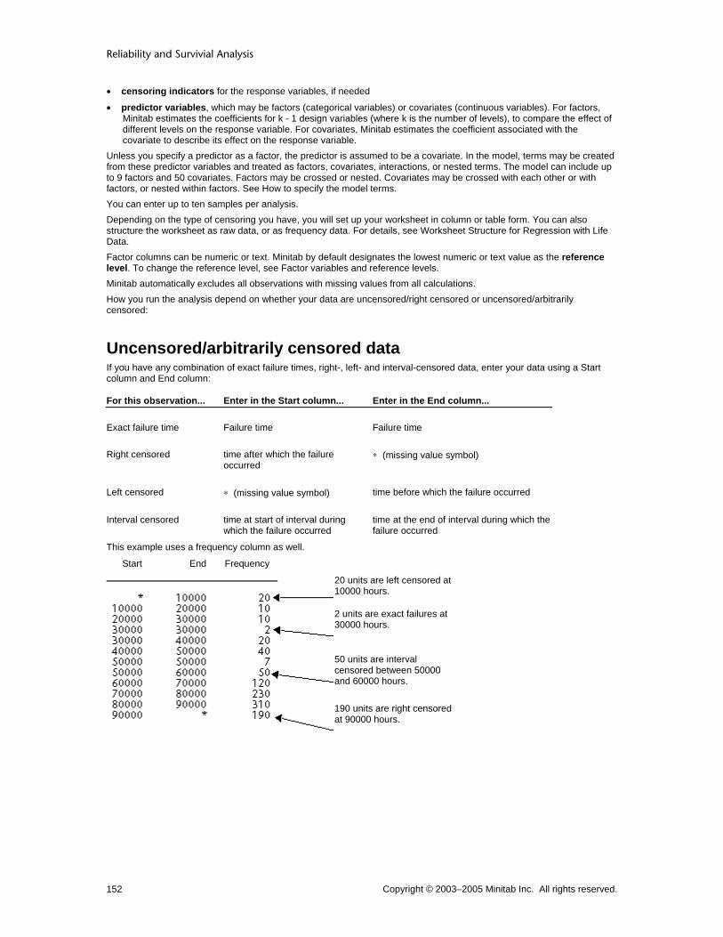
Reliability and Survivial Analysis
Copyright © 2003–2005 Minitab Inc. All rights reserved. 152
• censoring indicators for the response variables, if needed
• predictor variables, which may be factors (categorical variables) or covariates (continuous variables). For factors, Minitab estimates the coefficients for k - 1 design variables (where k is the number of levels), to compare the effect of different levels on the response variable. For covariates, Minitab estimates the coefficient associated with the covariate to describe its effect on the response variable.
Unless you specify a predictor as a factor, the predictor is assumed to be a covariate. In the model, terms may be created from these predictor variables and treated as factors, covariates, interactions, or nested terms. The model can include up to 9 factors and 50 covariates. Factors may be crossed or nested. Covariates may be crossed with each other or with factors, or nested within factors. See How to specify the model terms. You can enter up to ten samples per analysis. Depending on the type of censoring you have, you will set up your worksheet in column or table form. You can also structure the worksheet as raw data, or as frequency data. For details, see Worksheet Structure for Regression with Life Data. Factor columns can be numeric or text. Minitab by default designates the lowest numeric or text value as the reference level. To change the reference level, see Factor variables and reference levels. Minitab automatically excludes all observations with missing values from all calculations. How you run the analysis depend on whether your data are uncensored/right censored or uncensored/arbitrarily censored:
Uncensored/arbitrarily censored data If you have any combination of exact failure times, right-, left- and interval-censored data, enter your data using a Start column and End column:
For this observation... Enter in the Start column... Enter in the End column...
Exact failure time Failure time Failure time
Right censored time after which the failure occurred
∗ (missing value symbol)
Left censored ∗ (missing value symbol) time before which the failure occurred
Interval censored time at start of interval during which the failure occurred
time at the end of interval during which the failure occurred
This example uses a frequency column as well.
Start End Frequency
20 units are left censored at 10000 hours.
2 units are exact failures at 30000 hours.
50 units are interval censored between 50000 and 60000 hours.
190 units are right censored at 90000 hours.

Regression with Life Data
Copyright © 2003–2005 Minitab Inc. All rights reserved. 153
Uncensored/right censored data Enter two columns for each sample − one column of failure (or censoring) times and a corresponding column of censoring indicators.
Time Censor
The Time column contains failure times.
53 60 53 40 51 99 35 53 . . .
etc.
F F F F F C F F . . .
etc.
The Censor column contains the corresponding censoring indicators: an F designates an actual failure time; a C designates a unit that was removed from the test, and was thus censored.
Censoring indicators can be numbers, text, or date/time values. If you do not specify which value indicates censoring in the Censor subdialog box, Minitab assumes the lower of the two values indicates censoring, and the higher of the two values indicates an exact failure. The data column and associated censoring column must be the same length, although pairs of data/censor columns (each pair corresponds to a sample) can have different lengths.
Failure times The response data you gather for the regression with life data commands are the individual failure times. For example, you might collect failure times for units running at a given temperature. You might also collect samples under different temperatures, or under varying conditions of any combination of accelerating variables. Individual failure times are the same type of data used for Distribution Analysis. Life data is often censored or incomplete in some way. Suppose you are monitoring air conditioner fans to find out the percentage of fans that fail within a three-year warranty period. The table below describes the types of observations you can have:
Type of observation Description Example
Exact failure time You know exactly when the failure occurred.
The fan failed at exactly 500 days.
Right censored You only know that the failure occurred after a particular time.
The fan had not yet failed at 500 days.
Left censored You only know that the failure occurred before a particular time.
The fan failed sometime before 500 days.
Interval censored You only know that the failure occurred between two particular times.
The fan failed sometime between 475 and 500 days.
How you set up your worksheet depends, in part, on the type of censoring you have:
• When your data consist of exact failures and right-censored observations, see Uncensored/right censored data.
• When your data have a varied censoring scheme, see Uncensored/arbitrarily censored data.

Reliability and Survivial Analysis
Copyright © 2003–2005 Minitab Inc. All rights reserved. 154
To perform regression with uncensored/right censored data 1 Choose Stat > Reliability/Survival > Regression with Life Data.
2 In Variables/Start variables, enter up to ten columns of failure times (ten different samples).
3 If you have frequency columns, enter them in Freq. columns.
4 In Model, enter the model terms − see How to specify the model terms. If any of those predictors are factors, enter them again in Factors.
Note If you have no censored data, you can skip steps 5 & 6.
5 Click Censor.
6 In Use censoring columns, enter the censoring columns. The first censoring column is paired with the first data column, the second censoring column is paired with the second data column, and so on. By default, Minitab uses the lowest value in the censoring column to indicate a censored value. To use some other value, enter that value in Censoring value.
7 If you like, use any dialog box options, then click OK.
To perform regression with uncensored/arbitrarily censored data 1 Choose Stat > Reliability/Survival > Regression with Life Data.
2 Choose Responses are uncens/arbitrarily censored data.
3 In Variables/Start variables, enter up to ten columns of start times (ten different samples).
4 In End variables, enter up to ten columns of end times (ten different samples).
5 If you have frequency columns, enter them in Freq. columns.
6 In Model, enter the model terms − see How to specify the model terms. If any of those predictors are factors, enter them again in Factors.
7 If you like, use any dialog box options, then click OK.
Estimating the model parameters Minitab uses a modified Newton-Raphson algorithm to estimate the model parameters. If you like, you can enter your own parameters. In this case, no estimation is done; all results − such as the percentiles − are based on these parameters. When you let Minitab estimate the parameters from the data, you can optionally:
• enter starting values for the algorithm.
• change the maximum number of iterations for reaching convergence (the default is 20). Minitab obtains maximum likelihood estimates through an iterative process. If the maximum number of iterations is reached before convergence, the command terminates.
• estimate other model coefficients while holding the shape parameter (Weibull) or the scale parameter (other distributions) fixed at a specific value.
Why enter starting values for the algorithm? The maximum likelihood solution may not converge if the starting estimates are not in the neighborhood of the true solution, so you may want to specify what you think are good starting values for parameter estimates. In all cases, enter a column with entries that correspond to the model terms in the order you entered them in the Model box. With complicated models, find out the order of entries for the starting estimates column by looking at the regression table in the output.
Factor variables and reference levels You can enter numeric, text, or date/time factor levels. Minitab assigns one factor level to be the reference level, meaning that the estimated coefficients are interpreted relative to this level.

Regression with Life Data
Copyright © 2003–2005 Minitab Inc. All rights reserved. 155
Regression with Life Data creates a set of design variables for each factor in the model. If there are k levels, there will be k - 1 design variables and the reference level will be coded as 0. Here are two examples of the default coding scheme:
Factor A with 4 levels Factor B with 3 levels
(1 2 3 4) (High Low Medium)
reference level is 1
1 2 3 4
A1 0 1 0 0
A2 0 0 1 0
A3 0 0 0 1
reference level is High
High Low Medium
B1 0 1 0
B2 0 0 1
By default, Minitab designates the lowest numeric, date/time, or text value as the reference factor level. If you like, you can change this reference value in the Options subdialog box.
Multiple degrees of freedom test When you have a term with more than one degree of freedom, you can request a multiple degrees of freedom test. This procedure tests whether or not the term is significant. In other words: Is at least one of the coefficients associated with this term significantly different than zero?
Regression with Life Data - Censor Stat > Reliability/Survival > Regression with Life Data > Censor Allows you to specify the censoring columns.
Dialog box items Use censoring columns: If you have right censored data, enter the censoring columns. The first censoring column is paired with the first data column, the second censoring column is paired with the second data column, and so on. Censoring value: By default, Minitab uses the lowest value in the censoring column to indicate a censored observation. To use some other value, enter that value in Censoring value. Text values must be contained in double quotes.
Regression with Life Data - Estimate Stat > Reliability/Survival > Regression with Life Data > Estimate Percentile and Probability Estimation
Enter new predictor values: Choose to specify values for predictors to estimate percentiles and/or survival probabilities. Most often, you would enter the design value. You can enter the values separated by spaces, or one or more columns. Values (or columns) should be listed in the order that the corresponding variables appear in the model. Use predictor values in data (storage only): Choose to use the predictor values from the data to estimate percentiles and/or survival probabilities. Estimate percentiles for percents: Enter the percents for which you want to estimate percentiles. By default, Minitab estimates the 50th percentile. If you want to look at the beginning, middle, and end of the product's lifetime for a given predictor value, enter 10 50 90 (the 10th, 50th, 90th percentiles). Minitab then estimates how long it takes for 10% of the units to fail, 50% of the units to fail, and 90% of the units to fail.
Store percentiles Percentiles: Check to store the percentiles. Standard error: Check to store the standard error of the percentiles. Confidence limits: Check to store the confidence limits for the percentiles.
Estimate probabilities for times: Enter the times for which you want to estimate survival probabilities or cumulative failure probabilities.
Estimate survival probabilities: Choose to estimate survival probabilities. Estimate cumulative failure probabilities: Choose to estimate cumulative failure probabilities. Store probabilities
Probabilities: Check to store the survival probabilities or cumulative failure probabilities. Confidence limits: Check to store the confidence limits for the survival probabilities or cumulative failure probabilities.

Reliability and Survivial Analysis
Copyright © 2003–2005 Minitab Inc. All rights reserved. 156
Confidence level: Enter the confidence level for all of the confidence intervals. The default is 95%. Confidence intervals: Choose to use two-sided confidence intervals (the default) or just an upper or lower confidence interval.
To estimate percentiles and survival probabilities You can estimate percentiles and survival probabilities for new predictor values, or the values in your data. 1 In the Regression with Life Data dialog box, click Estimate. 2 Do one of the following:
• To enter new predictor values: In Enter new predictor values, enter a set of predictor values (or columns containing sets of predictor values) for which you want to estimate percentiles or survival probabilities. The predictor values must be in the same order as the main effects in the model. For an illustration, see Example of regression with life data.
• To use the predictor values in the data, choose Use predictor values in data (storage only). Because of the potentially large amount of output, Minitab stores the results in the worksheet rather then printing them in the Session window.
3 Do any of the following, then click OK: • To estimate percentiles, enter the percents or a column of percents in Estimate percentiles for percents. By
default, Minitab estimates the 50th percentile. If you want to look at the beginning, middle, and end of the product's lifetime for a given predictor value, enter 10 50 90 (the 10th, 50th, 90th percentiles). Minitab then estimates how long it takes for 10% of the units to fail, 50% of the units to fail, and 90% of the units to fail.
• To estimate survival probabilities, enter the times or a column of times in Estimate probabilities for times. For example, when you enter 70 (units in hours in this example), Minitab estimates the probability, for each predictor value, that the unit will survive past 70 hours.
Regression with Life Data - Graphs Stat > Reliability/Survival > Regression with Life Data > Graphs You can draw probability plots for the standardized and Cox-Snell residuals.
Dialog box items Probability plot for standardized residuals: Check to display a probability plot for standardized residuals. Exponential probability plot for Cox-Snell residuals: Check to display an exponential probability plot for Cox-Snell residuals. Display confidence intervals on probability plots: Check to display confidence intervals on the probability plots.
Note To change the method for calculating probability plot points, see Tools > Options > Individual Graphs > Probability Plots.
Probability plots for regression with life data The Regression with Life Data command draws probability plots for the standardized and Cox-Snell residuals. You can use these plots to assess whether a particular distribution fits your data. In general, the closer the points fall to the fitted line, the better the fit. Minitab provides one goodness-of-fit measure: the Anderson-Darling statistic. The Anderson-Darling statistic is useful in comparing the fit of different distributions. It measures the distances from the plot points to the fitted line; therefore, a smaller Anderson-Darling statistic indicates that the distribution provides a better fit.
To draw a probability plot of the residuals 1 In the Accelerated Life Testing or Regression with Life Data dialog box, click Graphs. 2 Do any of the following, then click OK:
• To plot the standardized residuals, check Probability plot for standardized residuals • To plot the Cox-Snell residuals, check Exponential probability plot for Cox-Snell residuals
Note To draw a probability plot with more options, store the residuals in the Storage subdialog box, then use the probability plot included with the Parametric Distribution Analysis commands.

Regression with Life Data
Copyright © 2003–2005 Minitab Inc. All rights reserved. 157
Regression with Life Data - Options Stat > Reliability/Survival > Regression with Life Data > Options
You can estimate the model parameters from the data or enter historical estimates − see Estimating the Model Parameters for more information. You can also change the reference level for a factor.
Dialog box items Estimate model parameters: Choose to estimate the model parameters from the data.
Use starting estimates: If you have starting estimates, enter one column to be used for all of the response variables, or a separate column for each response variable. The column(s) should contain one value for each coefficient in the regression table, in the order that the coefficients appear in the regression table. Maximum number of iterations: Enter a positive integer to specify the maximum number of iterations for the Newton-Raphson algorithm. Set shape (Weibull) or scale (other distributions) at: To estimate other model coefficients while holding the shape or scale parameter fixed, enter one value to be used as the shape or scale parameter for all of the response variables, or a number of values equal to the number of response variables.
Use historical estimates: Choose to enter your own estimates for the model parameters. Enter one column to be used for all of the response variables, or a separate column for each response variable. The column(s) should contain one value for each coefficient in the regression table, in the order that the coefficients appear in the regression table. Reference factor level (enter factor followed by level): For each factor you want to set the reference level for, enter a factor column followed by a value specifying the reference level. For text values, the value must be in double quotes. For date/time values, store the value as a constant and then enter the constant.
To control estimation of the parameters 1 In the Regression with Life Data dialog box, click Options. 2 Do one of the following:
• To estimate the model parameters from the data (the default), choose Estimate model parameters.
− To enter starting estimates for the parameters: In Use starting estimates, enter one column to be used for all of the response variables, or a number of columns equal to the number of response variables.
− To specify the Maximum number of iterations, enter a positive integer.
− To estimate other model coefficients while holding the shape parameter (Weibull) or the scale parameter (other distributions) fixed: In Set shape (Weibull) or scale (other distributions) at, enter one value to be used for all of the response variables, or a number of values equal to the number of response variables.
• To enter your own estimates for the model parameters, choose Use historical estimates and enter one column to be used for all of the response variables, or a number of columns equal to the number of response variables.
3 Click OK.
To change the reference factor level 1 In the Regression with Life Data dialog box, click Options. 2 In Reference factor level, for each factor you want to set the reference level for, enter a factor column followed by a
value specifying the reference level. For text values, the value must be in double quotes. For date/time values, store the value as a constant and then enter the constant.
3 Click OK.
Regression with Life Data - Results Stat > Reliability/Survival > Regression with Life Data > Results You can control the display of Session window output.
Dialog box items Control the Display of Results
Display nothing: Choose to suppress all printed output, but do all requested storage and display graphs. Response information, censoring information, regression table, log-likelihood, and goodness-of-fit: Choose to display the response and censoring information, the regression table, the log-likelihood, and goodness-of-fit measures.

Reliability and Survivial Analysis
Copyright © 2003–2005 Minitab Inc. All rights reserved. 158
In addition, table of percentiles and/or survival probabilities: Choose to display the output described above, plus a table of percentiles and/or survival probabilities (if requested in Regression with Life Data - Estimate). In addition, list of factor level values, tests for terms with more than one degree of freedom: Choose to display all of the output described above, plus a list of the factor level values, and a multiple degrees of freedom test.
Show log-likelihood for each iteration of algorithm: Check to display the log-likelihood at each iteration of the parameter estimation process.
To perform multiple degrees of freedom tests 1 In the Regression with Life Data dialog box, click Results. 2 Choose In addition, list of factor level values, tests for terms with more than 1 degree of freedom, then click
OK.
Regression with Life Data - Storage Stat > Reliability/Survival > Regression with Life Data > Storage You can store three types of residuals and information on the estimated equation.
Dialog box items Residuals Check any of the residual types below to store them in the worksheet.
Ordinary Standardized Cox-Snell
Information on Estimated Equation Estimated coefficients: Check to store the estimated coefficients. Standard error of estimates: Check to store the standard error of the estimated coefficients. Confidence limits for coefficients: Check to store the confidence limits for the coefficients. Variance/covariance matrix: Check to store the variance/covariance matrix for the estimated coefficients. Log-likelihood for last iteration: Check to store the log-likelihood for the last iteration.
Example of Regression with Life Data Suppose you want to investigate the deterioration of an insulation used for electric motors. You want to know if you can predict failure times for the insulation based on the plant in which it was manufactured, and the temperature at which the motor runs. It is known that an Arrhenius relationship exists between temperature and loge failure time.
You gather failure times at plant 1 and plant 2 for the insulation at four temperatures − 110, 130, 150, and 170° C. Because the motors generally run at between 80 and 100° C, you want to predict the insulation's behavior at those temperatures. To see how well the model fits, you will draw a probability plot based on the standardized residuals. 1 Open the worksheet INSULATE.MTW. 2 Choose Stat > Reliability/Survival > Regression with Life Data. 3 In Variables/Start variables, enter FailureT. 4 In Model, enter ArrTemp Plant. In Factors (optional), enter Plant. 5 Click Censor. In Use censoring columns, enter Censor, then click OK. 6 Click Estimate. In Enter new predictor values, enter ArrNewT NewPlant, then click OK. 7 Click Graphs. Check Probability plot for standardized residuals, then click OK in each dialog box.

Regression with Life Data
Copyright © 2003–2005 Minitab Inc. All rights reserved. 159
Session window output
Regression with Life Data: FailureT versus ArrTemp, Plant Response Variable: FailureT Censoring Information Count Uncensored value 66 Right censored value 14 Censoring value: Censor = C Estimation Method: Maximum Likelihood Distribution: Weibull Relationship with accelerating variable(s): Linear Regression Table Standard 95.0% Normal CI Predictor Coef Error Z P Lower UpperIntercept -15.3411 0.950822 -16.13 0.000 -17.2047 -13.4775ArrTemp 0.839255 0.0339710 24.71 0.000 0.772673 0.905837Plant 2 -0.180767 0.0845721 -2.14 0.033 -0.346525 -0.0150083Shape 2.94309 0.270658 2.45768 3.52439 Log-Likelihood = -562.525 Table of Percentiles Standard 95.0% Normal CI Percent ArrTemp Plant Percentile Error Lower Upper 50 32.8600 1 182094 32466.2 128390 258261 50 32.8600 2 151981 25286.6 109690 210578 50 31.0988 1 41530.4 5163.76 32548.4 52990.9 50 31.0988 2 34662.5 3913.87 27781.0 43248.6

Reliability and Survivial Analysis
Copyright © 2003–2005 Minitab Inc. All rights reserved. 160
Graph window output:
Interpreting the results From the Regression Table, you get the coefficients for the regression model. For the Weibull distribution, here is the equation that describes the relationship between temperature and failure time for the insulation for plant 1 and 2, respectively:
Loge (failure time) = −15.3411 + 0.83925 (ArrTemp) + 1/2.9431
Loge (failure time) = −15.52187 + 0.83925 (ArrTemp) + 1/2.9431
where = the pth percentile of the error distribution ArrTemp = 11604.83/(Temp + 273.16) The Table of Percentiles displays the 50th percentiles for the combinations of temperatures and plants that you entered. The 50th percentile is a good estimate of how long the insulation will last in the field:
• For motors running at 80° C, insulation from plant 1 lasts about 182093.6 hours or 20.77 years; insulation from plant 2 lasts about 151980.8 hours or 17.34 years.
• For motors running at 100° C, insulation from plant 1 lasts about 41530.38 hours or 4.74 years; insulation from plant 2 lasts about 34662.51 hours or 3.95 years.
As you can see from the low p-values, the plants are significantly different at the α = .05 level, and temperature is a significant predictor. The probability plot for standardized residuals will help you determine whether the distribution, transformation, and equal shape (Weibull or exponential) or scale parameter (other distributions) assumption is appropriate. Here, the plot points fit the fitted line adequately; therefore you can assume the model is appropriate.

Regression with Life Data
Copyright © 2003–2005 Minitab Inc. All rights reserved. 161
Default output The default output consists of the regression table, which displays:
• the estimated coefficients for the regression model and their − standard errors. − Z-values and p-values. The Z-test tests that the coefficient is significantly different than 0; in other words, is it a
significant predictor? − 95% confidence interval.
• the Scale parameter, a measure of the overall variability, and its − standard error. − 95% confidence interval.
• the Shape parameter (Weibull or exponential) or Scale parameter (other distributions), a measure of the overall variability, and its − standard error. − 95% confidence interval.
• the log-likelihood.

Probit Analysis
Copyright © 2003–2005 Minitab Inc. All rights reserved. 163
Probit Analysis Probit Analysis Overview A probit study consists of imposing a stress (or stimulus) on a number of units, then recording whether the unit failed or not. Probit analysis differs from accelerated life testing in that the response data is binary (success or failure), rather than an actual failure time. In the engineering sciences, a common experiment would be destructive inspecting. Suppose you are testing how well submarine hull materials hold up when exposed to underwater explosions. You subject the materials to various magnitudes of explosions, then record whether or not the hull cracked. In the life sciences, a common experiment would be the bioassay, where you subject organisms to various levels of a stress and record whether or not they survive. Probit analysis can answer these kinds of questions: For each hull material, what shock level cracks 10% of the hulls? What concentration of a pollutant kills 50% of the fish? Or, at a given pesticide application, what's the probability that an insect dies?
Probit Analysis Stat > Reliability/Survival > Probit Analysis Use probit analysis when you want to estimate percentiles, survival probabilities, and cumulative failure probabilities for the distribution of a stress, and draw probability plots. When you enter a factor and choose a Weibull, lognormal, or loglogistic distribution, you can also compare the potency of the stress under different conditions. Minitab calculates the model coefficients using a modified Newton-Raphson algorithm.
Dialog box items Response in success/trial format: Choose if your data is in success/trial format.
Number of successes: Enter the column containing the number of successes. Number of trials: Enter the column containing the number of trials.
Response in response/frequency format: Choose if your data is in response/frequency format. Response: Enter the column that contains the response data.
with frequency (optional): Optionally, enter a column of frequencies. Stress (stimulus): Enter a column of stress or stimulus levels. Factor (optional): Enter one column of factor levels. Assumed distribution: Click the drop-down arrow and choose one of seven common lifetime distributions. Choices include the normal (default), lognormal, logistic, loglogistic, Weibull, and smallest extreme value distributions.
Data - Probit Analysis Enter the following columns in the worksheet:
• two columns containing the response variable, set up in success/trial or response/frequency format
• one column containing a stress variable (treated as a covariate in Minitab)
• (optional) one column containing a factor

Reliability and Survivial Analysis
Copyright © 2003–2005 Minitab Inc. All rights reserved. 164
Response variable The response data is binomial, so you have two possible outcomes, success or failure. You can enter the data in either success/trial or response/frequency format. Here is the same data arranged both ways:
Success/trial format Response/frequency format
Temp Success Trials Temp Response Frequency
80 2 10 80 1 2
120 4 10 80 0 8
140 7 10 120 1 4
160 9 10 120 0 6
140 1 7
140 0 3
160 1 9
160 0 1
The Success column contains the number of successes. The Trials column contains the number of observations. For example, when Temp = 140, there were seven successes and three failures.
The Response column contains values which indicate whether the unit succeed or failed. The higher value corresponds to a success. The Frequency column indicates how many times that observation occurred. For example, when Temp = 160, there were nine successes and one failure.
Factors Text categories (factor levels) are processed in alphabetical order by default. If you wish, you can define your own order − see Ordering Text Categories.
To perform a probit analysis How you run the analysis depend on whether your worksheet is in "success/trial" or "response/frequency" format. 1 Choose Stat > Reliability/Survival > Probit Analysis. 2 Do one of the following:
• Choose Responses in success/trial format.
1 In Number of successes, enter one column of successes.
2 In Number of trials, enter one column of trials. • Choose Responses in response/frequency format.
1 In Response, enter one column of response values.
2 If you have a frequency column, enter the column in with frequency.
3 In Stress (stimulus), enter one column of stress or stimulus levels. 4 If you like, use any of the dialog box options, then click OK.
Probit model and distribution function Minitab provides three main distributions − normal, logistic, and extreme value − allowing you to fit a broad class of binary response models. You can take the log of the stress to get the lognormal, loglogistic, and Weibull distributions, respectively. This class of models (for the situation with no factor) is defined by:
where
= the probability of a response for the jth stress level
g(yj) = the distribution function (described below)
β0 = the constant term
xj = the jth level of the stress variable

Probit Analysis
Copyright © 2003–2005 Minitab Inc. All rights reserved. 165
β = unknown coefficient associated with the stress variable
c = natural response rate
The distribution functions are outlined below:
Distribution Distribution function Mean Variance logistic
0 pi**2 / 3
normal
0 1
extreme value
(Euler constant)
pi**2 / 6
Here, pi in the Variance column of the table is 3.14159. The distribution function you choose should depend on your data. You want to choose a distribution function that results in a good fit to your data. Goodness-of-fit statistics can be used to compare fits using different distributions. Certain distributions may be used for historical reasons or because they have a special meaning in a discipline.
Estimating the model parameters Minitab uses a modified Newton-Raphson algorithm to estimate the model parameters. If you like, you can enter historical estimates for these parameters. In this case, no estimation is done; all results − such as the percentiles − are based on these historical estimates. When you let Minitab estimate the parameters from the data, you can optionally:
• enter starting values for the algorithm.
• change the maximum number of iterations for reaching convergence (the default is 20). Minitab obtains maximum likelihood estimates through an iterative process. If the maximum number of iterations is reached before convergence, the command terminates.
Why enter starting values for the algorithm? The maximum likelihood solution may not converge if the starting estimates are not in the neighborhood of the true solution, so you may want to specify what you think are good starting values for parameter estimates.
Factor variables and reference levels You can enter numeric, text, or date/time factor levels. Minitab needs to assign one factor level to be the reference level, meaning that the estimated coefficients are interpreted relative to this level. Probit analysis creates a set of design variables for the factor in the model. If there are k levels, there will be k-1 design variables and the reference level will be coded with all 0's. Here are two examples of the default coding scheme:
Factor A with 4 levels Factor B with 3 levels
(1 2 3 4) (High Low Medium)
reference level is 1
1 2 3 4
A1 0 1 0 0
A2 0 0 1 0
A3 0 0 0 1
reference level is High
High Low Medium
B1 0 1 0
B2 0 0 1
By default, Minitab designates the lowest numeric, date/time, or text value as the reference factor level. If you like, you can change this reference value in the Options subdialog box.
Natural response rate The regression table includes the natural response rate − the probability that a unit fails without being exposed to any of the stress. This statistic is used in situations with high mortality or high failure rates. For example, you might want to know the probability that a young fish dies without being exposed to a certain pollutant. If the natural response rate is greater than 0, you may want to consider the fact that the stress does not cause all of the deaths in the analysis. You can choose to estimate the natural response rate from the data, or set the value. You would set the value when you have a historical estimate, or to use as a starting value for the algorithm.

Reliability and Survivial Analysis
Copyright © 2003–2005 Minitab Inc. All rights reserved. 166
Percentiles At what stress level do half of the units fail? How much pesticide do you need to apply to kill 90% of the insects? You are looking for percentiles. Common percentiles used are the 10th, 50th, and 90th percentiles, also known in the life sciences as the ED 10, ED 50 and ED 90 (ED = effective dose). The probit analysis automatically displays a table of percentiles in the Session window, along with 95% fiducial confidence intervals. You can also request:
• additional percentiles to be added to the table
• normal approximation rather than fiducial confidence intervals
• a confidence level other than 95% The Percentile column contains the stress level required for the corresponding percent of the events to occur. In this example, you exposed light bulbs to various voltages and recorded whether or not the bulb burned out before 800 hours. Table of Percentiles
Standard 95.0% Fiducial CI
Percent Percentile Error Lower Upper
1 104.9931 1.3715 101.9273 107.3982
2 106.9313 1.2661 104.1104 109.1598
3 108.1795 1.1997 105.5144 110.2980
4 109.1281 1.1504 106.5795 111.1656
As shown in the first and second columns of the first row, at 104.9931 volts, 1% of the bulbs burn out before 800 hours.
Survival and cumulative probabilities What is the probability that a submarine hull will survive a given strength of shock? At a given pesticide application, what is the probability that an insect survives? You are looking for survival probabilities − estimates of the proportion of units that survive at a certain stress level. When you request survival probabilities, they are displayed in a table in the Session window. In this example, we exposed light bulbs to various voltages and recorded whether or not the bulb burned out before 800 hours. Then we requested a survival probability for light bulbs subjected to 117 volts: Table of Percentiles
95.0% Fiducial CI
Stress Probability Lower Upper
117.0000 0.7692 0.6224 0.8825
The probability of a bulb lasting past 800 hours is 0.7692 at 117 volts. The cumulative failure probabilities are the likelihood of failing rather than surviving. In this case, the probability of failing before 800 hours at 117 volts is 0.2308.
Probit Analysis - Estimate Stat > Reliability/Survival > Probit Analysis > Estimate You can estimate additional percentiles, survival probabilities, and cumulative failure probabilities. You can
• estimate percentiles for the percents you specify. These percentiles are added to the default table of percentiles.
• estimate survival probabilities for the stress values you specify.
• estimate cumulative failure probabilities for the stress values you specify. You can also change the method of estimation for the confidence intervals and the level of confidence.

Probit Analysis
Copyright © 2003–2005 Minitab Inc. All rights reserved. 167
Dialog box items Estimate percentiles for these additional percents: Enter one or more percents or a column of percent values. Estimate probabilities for these stress values: Enter one or more stress values or columns of stress values.
Estimate survival probabilities: Choose to estimate survival probabilities. Estimate cumulative failure probabilities: Choose to estimate cumulative failure probabilities.
Confidence Intervals Fiducial: Choose to display fiducial (default) confidence intervals. Normal approximation: Choose to display confidence intervals obtained with a normal approximation.
Confidence level: Enter a confidence level for all of the confidence intervals. The default is 95%. Confidence intervals: Choose to use two-sided confidence intervals (the default) or just an upper or lower confidence interval.
To request survival probabilities 1 In the Probit Analysis main dialog box, click Estimate. 2 In Estimate probabilities for these stress values, enter one or more stress values or columns of stress values.
Click OK.
Probit Analysis - Graphs Stat > Reliability/Survival > Probit Analysis > Graphs You can draw probability, survival, and cumulative failure plots. You can also plot the Pearson or deviance residuals versus the event probability. Use these plots to identify poorly fit observations.
Dialog box items Probability Plot: Check to display a probability plot. Survival plot: Check to display a survival plot. Cumulative failure plot: Check to display a cumulative failure plot. Display confidence intervals on above plots: Check to display confidence intervals on the probability, survival, and cumulative failure plots. Show graphs of different variables or by levels: Choose to display the graphs overlaid on the same page or on separate pages. Pearson residuals versus event probability: Check to display a plot of the Pearson residuals versus the event probability. Deviance residuals versus event probability: Check to display a plot of the deviance residuals versus the event probability.
To draw a survival plot 1 In the Probit Analysis dialog box, click Graphs. 2 Check Survival plot.
3 If you like, turn off the 95% confidence interval − uncheck Display confidence intervals on above plots. Click OK.
4 If you like, change the confidence level for the 95% confidence interval − click Estimate. In Confidence level, enter a value. Click OK.
Probability plots A probability plot displays the percentiles. You can use the probability plot to assess whether a particular distribution fits your data. In general, the closer the points fall to the fitted line, the better the fit. When you have more than one factor level, lines and confidence intervals are drawn for each level. If the plot looks cluttered, you can turn off the confidence intervals in the Graphs subdialog box. You can also change the confidence level for the 95% confidence by entering a new value in the Estimate subdialog box.

Reliability and Survivial Analysis
Copyright © 2003–2005 Minitab Inc. All rights reserved. 168
Survival plots Survival plots display the survival probabilities versus stress. Each point on the plot represents the proportion of units surviving at a stress level. The survival curve is surrounded by two outer lines − the 95% confidence interval for the curve, which provide reasonable values for the "true" survival function.
Probit Analysis - Options Stat > Reliability/Survival > Probit Analysis > Options You can choose to estimate model parameters and the natural response rate from the data or enter values, define the event and reference factor level, and change the number of groups for the Hosmer-Lemeshow Test.
Dialog box items Estimate model parameters: Choose to estimate the model parameters from the data (the default).
Use starting estimates: Enter a column that contains starting values for model parameters. The column should include one starting value for each coefficient in the regression table. Values should be listed in the order that they appear in the regression table. Maximum number of iterations: Enter a number to change the maximum number of iterations for reaching convergence (the default is 20). Minitab obtains maximum likelihood estimates through an iterative process. If the maximum number of iterations is reached before convergence, the command terminates.
Use historical estimates: Enter a column that contains historical estimates for the model parameters. The column should include one value for each coefficient in the regression table. Values should be listed in the order that they appear in the regression table. Natural response rate
Estimate from data: Check to estimate the natural response rate. Set value: Enter a value for the estimate of the natural response rate. If Estimate from data is checked, this value will be used as a starting value for the algorithm for estimating the natural response rate. If Estimate from data is unchecked, this value will be used as the natural response rate.
Reference Options Event: If you have response/frequency data, you can enter a value to define the occurrence of a success. If you do not enter a value, the highest value in the column is used. Reference factor level: Enter a reference level for the factor. Otherwise, the lowest value in the column is used.
Option for Hosmer-Lemeshow Test: To see the results of this test, you must choose the option to display all results in the Probit Analysis - Results dialog box.
Number of groups: Enter the number of groups for the Hosmer-Lemeshow goodness-of-fit test. By default, this test bins the data into 10 groups.
To control estimation of the parameters 1 In the Probit Analysis main dialog box, click Options. 2 Do one of the following, then click OK:
• To estimate the model parameters from the data (the default), choose Estimate model parameters.
− To enter starting estimates for the parameters: In Use starting estimates, enter one starting value for each coefficient in the regression table. Enter the values in the order that they appear in the regression table.
Note Do not enter a starting value for the natural response rate here.
− To specify the maximum number of iterations, enter a positive integer. • To enter your own estimates for the model parameters, choose Use historical estimates and enter one starting
value for each coefficient in the regression table. Enter the values in the order that they appear in the regression table.
Probit Analysis - Results Stat > Reliability/Survival > Probit Analysis > Results You can control the display of Session window output.

Probit Analysis
Copyright © 2003–2005 Minitab Inc. All rights reserved. 169
Dialog box items Control the Display of Results Choose one of the options below to control display of Session window output.
Display nothing Choose to suppress display of the results. Response information, regression table, test for equal slopes, log-likelihood, multiple DF test and 2 goodness-of-fit tests Choose to display information about the response, the regression table, the test for equal slopes (if the model contains a factor), the log-likelihood, the multiple degree of freedom test (if the model contains a factor with more than two levels), and the Pearson and Deviance goodness-of-fit tests. In addition, distribution parameter estimates, table of percentiles and survival probabilities: Choose to display the distribution parameter estimates, table of percentiles and/or survival probabilities (if requested in Probit Analysis - Estimate). In addition, characteristic of distribution and the Hosmer-Lemeshow goodness-of-fit test: You must choose this option in order to see the results of the Hosmer-Lemeshow test.
Show log-likelihood for each iteration of algorithm: Check to display the log-likelihood at each iteration of the parameter estimation process.
To modify the table of percentiles 1 In the Probit Analysis main dialog box, click Estimate. 2 Do any of the following, then click OK:
• In Estimate percentiles for these additional percents, enter the percents or a column of percents. • Choose Normal approximation to request normal approximation rather than fiducial confidence intervals. • Change the confidence level for the percentiles (default is 95%): In Confidence level, enter a value. This changes
the confidence level for all confidence intervals.
Probit Analysis - Storage Stat > Reliability/Survival > Probit Analysis > Storage You can store the Pearson and deviance residuals, characteristics of the fitted distribution, and information on the estimated equation.
Dialog box items Enter number of levels in factor variable: If all of the samples are stacked in one column, enter the number of levels the column of grouping indicators contains. Residuals Choose to store one or both of the residual types below:
Pearson Deviance
Characteristics of Fitted Distribution Choose to store any of the fitted distribution characteristics below: Percentiles: Check to store the percentiles. Percents for percentiles: Check to store the percents associated with the percentiles. Standard error of percentiles: Check to store the standard error of the percentiles. Confidence limits for percentiles: Check to store the confidence interval limits for the percentiles. Stress for probabilities: Check to store the stress for survival probabilities or cumulative failure probabilities. Survival probabilities: Check to store the survival probabilities. Confidence limits for survival probabilities: Check to store the confidence limits for survival probabilities. Cumulative failure probabilities: Check to store the cumulative failure probabilities. Confidence limits for cumulative failure probabilities: Check to store the confidence limits for cumulative failure probabilities.
Information on Estimated Equation Choose to store any of the information on the estimated equation below: Event probability: Check to store the event probability. Estimated coefficients: Check to store the estimated coefficients. Standard error of estimates: Check to store the standard error of the estimated coefficients. Variance/covariance matrix: Check to store the variance/covariance matrix for the estimated coefficients. Natural response rate: Check to store the natural response rate. Standard error of natural response: Check to store the standard error of the natural response rate.

Reliability and Survivial Analysis
Copyright © 2003–2005 Minitab Inc. All rights reserved. 170
Log-likelihood for last iteration: Check to store the log-likelihood for the last iteration.
Example of a Probit Analysis Suppose you work for a light bulb manufacturer and have been asked to determine bulb life for two types of bulbs at typical household voltages. The typical line voltage entering a house is 117 volts + 10% (or 105 to 129 volts). You subject the two bulbs to five stress levels within that range: 108, 114, 120, 126, and 132 volts, and define a success as: The bulb fails before 800 hours. 1 Open the worksheet LIGHTBUL.MTW. 2 Choose Stat > Reliability/Survival > Probit Analysis. 3 Choose Response in success/trial format. 3 In Number of successes, enter Blows. In Number of trials, enter Trials. 4 In Stress (stimulus), enter Volts. 5 In Factor (optional), enter Type. 6 From Assumed distribution, choose Weibull. 7 Click Estimate. In Estimate probabilities for these stress values, enter 117, then click OK. 8 Click Graphs. Uncheck Display confidence intervals on above plots. Click OK in each dialog box.
Session Window Output:
Probit Analysis: Blows, Trials versus Volts, Type Distribution: Weibull Response Information Variable Value Count Blows Success 192 Failure 308 Trials Total 500 Factor Information Factor Levels Values Type 2 A, B Estimation Method: Maximum Likelihood Regression Table Standard Variable Coef Error Z P Constant -97.0190 7.67326 -12.64 0.000 Volts 20.0192 1.58695 12.61 0.000 Type B 0.179368 0.159832 1.12 0.262 Natural Response 0 Test for equal slopes: Chi-Square = 0.258463 DF = 1 P-Value = 0.611 Log-Likelihood = -214.213 Goodness-of-Fit Tests Method Chi-Square DF P Pearson 2.51617 7 0.926 Deviance 2.49188 7 0.928 Type = A

Probit Analysis
Copyright © 2003–2005 Minitab Inc. All rights reserved. 171
Tolerance Distribution Parameter Estimates Standard 95.0% Normal CI Parameter Estimate Error Lower Upper Shape 20.0192 1.58695 17.1384 23.3842 Scale 127.269 0.737413 125.832 128.722 Table of Percentiles 95.0% Fiducial Standard CI Percent Percentile Error Lower Upper 1 101.141 1.84244 96.9868 104.341 2 104.731 1.63546 101.043 107.573 3 106.901 1.50897 103.501 109.527 4 108.476 1.41713 105.287 110.946 5 109.720 1.34490 106.698 112.068 6 110.753 1.28539 107.868 113.001 7 111.639 1.23483 108.872 113.802 8 112.416 1.19095 109.752 114.506 9 113.110 1.15225 110.536 115.135 10 113.737 1.11771 111.246 115.706 20 118.082 0.898619 116.121 119.700 30 120.881 0.790097 119.201 122.342 40 123.069 0.735850 121.550 124.472 50 124.960 0.717911 123.523 126.372 60 126.714 0.728520 125.299 128.191 70 128.454 0.764984 127.010 130.050 80 130.330 0.830361 128.802 132.108 90 132.683 0.943441 130.989 134.754 91 132.980 0.959732 131.261 135.092 92 133.298 0.977596 131.551 135.455 93 133.641 0.997402 131.864 135.848 94 134.018 1.01968 132.206 136.280 95 134.439 1.04522 132.587 136.765 96 134.922 1.07534 133.023 137.323 97 135.500 1.11242 133.542 137.993 98 136.243 1.16159 134.207 138.857 99 137.358 1.23831 135.198 140.159 Table of Survival Probabilities 95.0% Fiducial CI Stress Probability Lower Upper 117 0.830608 0.780679 0.878549 Type = B Tolerance Distribution Parameter Estimates Standard 95.0% Normal CI Parameter Estimate Error Lower Upper Shape 20.0192 1.58695 17.1384 23.3842 Scale 126.134 0.704348 124.761 127.522

Reliability and Survivial Analysis
Copyright © 2003–2005 Minitab Inc. All rights reserved. 172
Table of Percentiles 95.0% Fiducial Standard CI Percent Percentile Error Lower Upper 1 100.239 1.86171 96.0399 103.471 2 103.797 1.65621 100.059 106.673 3 105.947 1.53027 102.496 108.607 4 107.508 1.43857 104.267 110.012 5 108.742 1.36626 105.666 111.123 6 109.765 1.30652 106.828 112.045 7 110.643 1.25563 107.823 112.837 8 111.413 1.21135 108.697 113.533 9 112.101 1.17218 109.476 114.156 10 112.723 1.13711 110.180 114.720 20 117.028 0.910842 115.029 118.659 30 119.803 0.792908 118.102 121.256 40 121.972 0.727988 120.452 123.344 50 123.845 0.698947 122.429 125.203 60 125.584 0.698766 124.211 126.984 70 127.309 0.725223 125.925 128.806 80 129.168 0.781440 127.719 130.828 90 131.500 0.885656 129.901 133.434 91 131.794 0.901010 130.172 133.767 92 132.109 0.917912 130.461 134.125 93 132.449 0.936720 130.773 134.513 94 132.822 0.957949 131.114 134.939 95 133.240 0.982380 131.493 135.418 96 133.719 1.01129 131.927 135.969 97 134.292 1.04700 132.444 136.631 98 135.028 1.09453 133.104 137.484 99 136.132 1.16901 134.090 138.772 Table of Survival Probabilities 95.0% Fiducial CI Stress Probability Lower Upper 117 0.800867 0.745980 0.854567 Table of Relative Potency Factor: Type Relative 95.0% Fiducial CI Comparison Potency Lower Upper A VS B 0.991080 0.975363 1.00678

Probit Analysis
Copyright © 2003–2005 Minitab Inc. All rights reserved. 173
Graph window output:
Interpreting the results The goodness-of-fit tests (p-values = 0.926, 0.928) and the probability plot suggest that the Weibull distribution fits the data adequately. Since the test for equal slopes is not significant (p-value = .611), the comparison of light bulbs will be similar regardless of the voltage level. In this case, the light bulbs A and B are not significantly different because the coefficient associated with type B is not significantly different than 0 (p-value = .262). At 117 volts, what percentage of the bulbs lasts beyond 800 hours? Eight-three percent of the bulb A's and 80% of the bulb B's last beyond 800 hours. At what voltage do 50% of the bulbs fail before 800 hours? The table of percentiles shows you that 50% of bulb A's fail before 800 hours at 124.96 volts; 50% of bulb B's fail before 800 hours at 123.85 volts.
Probit Analysis - Output The default output consists of:
• the response information
• the factor information
• the regression table, which includes the estimated coefficients and their − standard errors. − Z-values and p-values. The Z-test tests that the coefficient is significantly different than 0; in other words, is it a
significant predictor? − natural response rate − the probability that a unit fails without being exposed to any of the stress.
• the test for equal slopes, which tests that the slopes associated with the factor levels are significantly different.
• the log-likelihood from the last iteration of the algorithm.
• two goodness-of-fit tests, which evaluate how well the model fits the data. The null hypothesis is that the model fits the data adequately. Therefore, the higher the p-value the better the model fits the data.
• the parameter estimates for the distribution and their standard errors and 95% confidence intervals. The parameter estimates are transformations of the estimated coefficients in the regression table.

Reliability and Survivial Analysis
Copyright © 2003–2005 Minitab Inc. All rights reserved. 174
• the table of percentiles, which includes the estimated percentiles, standard errors, and 95% fiducial confidence intervals.
• the probability plot, which helps you to assess whether the chosen distribution fits your data.
• the relative potency − compares the potency of a stress for two levels of a factor. To get this output, you must have a factor, and choose a Weibull, lognormal, or loglogistic distribution. Suppose you want to compare how the amount of voltage affects two types of light bulbs, and the relative potency is .98. This means that light bulb 1 running at 117 volts would fail at approximately the same time as light bulb 2 running at 114.66 volts (117 x .98).

References, Reliability and Survival
Copyright © 2003–2005 Minitab Inc. All rights reserved. 175
References - Reliability and Survival Analysis [1] R.B. D'Agostino and M.A. Stephens (1986). Goodness-of-Fit Techniques, Marcel Dekker. [2] J.D. Kalbfleisch and R.L. Prentice (1980). The Statistical Analysis of Failure Time Data, John Wiley & Sons. [3] D. Kececioglu (1991). Reliability Engineering Handbook, Vols 1 and 2, Prentice Hall. [4] J.F. Lawless (1982). Statistical Models and Methods for Lifetime Data, John Wiley & Sons, Inc. [5] W.Q. Meeker and L.A. Escobar (1998). Statistical Methods for Reliability Data, John Wiley & Sons, Inc. [6] W. Murray, Ed. (1972). Numerical Methods for Unconstrained Optimization, Academic Press. [7] W. Nelson (1982). Applied Life Data Analysis, John Wiley & Sons. [8] W. Nelson (1985). "Weibull Analysis of Reliability Data with Few or No Failures," Journal of Quality Technology 17, 3,
pp. 140-146. [9] R. Peto (1973). "Experimental Survival Curves for Interval-censored Data," Applied Statistics 22, pp. 86-91. [10] B.W. Turnbull (1976). "The Empirical Distribution Function with Arbitrarily Grouped, Censored and Truncated Data,"
Journal of the Royal Statistical Society 38, pp. 290-295. [11] B.W. Turnbull (1974). "Nonparametric Estimation of a Survivorship Function with Doubly Censored Data," Journal of
the American Statistical Association 69, 345, pp. 169-173. [12] J.T. Kvaloy and B.H. Lindqvist (1998). "TTT-based tests for trend in repairable systems data," Reliability Engineering
and System Safety 60, pp. 13-28. [13] W. Nelson (1990). Accelerated Testing, John Wiley & Sons. [14] S.E. Rigdon and A.P. Basu (2000). Statistical Methods for the Reliability of Repairable Systems, John Wiley & Sons. [15] W. Nelson (2003). Recurrent Events Data Analysis for Product Repairs, Disease Recurrences, and Other
Applications, ASA-SIAM Seires on Statistics and Applied Probability.


Index
Copyright © 2003–2005 Minitab Inc. All rights reserved. 177
Index A
Accelerated life test model.......................................... 18 Accelerated Life Test Plans ........................................ 16
Accelerated Life Test Plans (Stat menu)................. 16 Accelerated Life Testing ........................................... 141
Accelerated Life Testing (Stat menu) .................... 141 Anderson-Darling statistic ..................................... 24, 64 Arrhenius transformation........................................... 143 C
Censored data .7, 8, 24, 26, 31, 35, 54, 67, 73, 78, 103, 115
Cumulative failure plot .......................................... 43, 91 Parametric distribution analysis......................... 43, 91
D
Demonstration Test Plans............................................. 8 Demonstration Test Plans (Stat menu) ..................... 8
Distribution ID Plot (Arbitrary Censoring).................... 26 Distribution ID Plot (Stat menu)............................... 26
Distribution ID Plot (Right Censoring) ......................... 66 Distribution ID Plot (Stat menu)............................... 66
Distribution Overview Plot (Arbitrary Censoring) ........ 31 Distribution Overview Plot (Stat menu) ................... 31
Distribution Overview Plot (Right Censoring) ............. 72 Distribution Overview Plot (Stat menu) ................... 72
Duane plot................................................................. 125 E
Estimation methods for reliability analysis ...... 23, 39, 88 Least squares method....................................... 39, 88 Maximum likelihood method.............................. 39, 88 Parametric growth curves...................................... 122
Estimation Test Plans ................................................. 12 Estimation Test Plans (Stat menu).......................... 12
Event plot .......................................................... 124, 131 F
Failure censoring .......................................................... 7 Frequency column ...................................................... 65 G
Goodness-of-fit statistics....................................... 24, 64 Growth curve data..................................... 115, 116, 117 Growth curves................................................... 118, 130
Nonparametric Growth Curves.............................. 130 Parametric Growth Curve...................................... 118
H
Hazard plots............................................ 43, 58, 92, 105 Nonparametric analysis................................... 58, 105 Parametric analysis ........................................... 43, 92
I Inverse temperature transformation ......................... 143 L
Least squares estimates....................................... 39, 88 Loge (power) transformation .................................... 143 M
Maximum likelihood estimates.............................. 39, 88 Mean cumulative difference function plot ................. 133 Mean cumulative function plot .......................... 123, 132 M-failure test plan......................................................... 9 Multiple failure modes............................. 38, 55, 80, 104
Nonparametric distribution analysis ................ 55, 104 Parametric distribution analysis ........................ 38, 80
N
Natural response rate ............................................... 165 Nonparametric Distribution Analysis (Arbitrary
Censoring) .............................................................. 53 Nonparametric Distribution Analysis (Stat menu) ... 53
Nonparametric Distribution Analysis (Right Censoring).............................................................................. 102 Nonparametric Distribution Analysis (Stat menu) . 102
Nonparametric Growth Curve................................... 130 Nonparametric Growth Curve (Stat menu) ........... 130
P
Parametric Distribution Analysis (Arbitrary Censoring)................................................................................ 35 Parametric Distribution Analysis (Stat menu) ......... 35
Parametric Distribution Analysis (Right Censoring) ... 77 Parametric Distribution Analysis (Stat menu) ......... 77
Parametric Growth Curve ......................................... 118 Parametric Growth Curve (Stat menu) ................. 118
Pearson correlation coefficient ............................. 24, 64 Percentiles............................................................ 37, 79
Accelerated life testing.......................................... 144 Parametric distribution analysis ........................ 37, 79 Probit analysis....................................................... 166
POP graph.................................................................. 10 Probability of passing the demonstration test plot ...... 10 Probability Plot.............................. 44, 93, 146, 156, 167
Probability Plot (Reliability/Survival) 44, 93, 146, 156, 167
Probit Analysis.......................................................... 163 Probit Analysis (Stat menu) .................................. 163
R
Regression with Life Data ........................................ 151 Regression with Life Data (Stat menu) ................. 151
Relation plot.............................................................. 146 Repairable systems analysis ............................ 118, 130

Reliability and Survivial Analysis
Copyright © 2003–2005 Minitab Inc. All rights reserved. 178
S
Stacked data ......................................................... 25, 65 Survival plots................................... 45, 59, 94, 106, 107
Comparing survival plots ....................................... 107 Nonparametric distribution analysis ................ 59, 106 Parametric distribution analysis......................... 45, 94 Probit analysis ....................................................... 168
Survival probabilities ............................. 37, 80, 144, 166 Accelerated life testing .......................................... 144 Parametric distribution analysis......................... 37, 80 Probit analysis ....................................................... 166
T
Test plans ......................................................... 8, 12, 16 Accelerated life test plans....................................... 16 Demonstration test plans .......................................... 8 Estimation test plans............................................... 12
Time censoring ............................................................. 8 Total time on test plot ............................................... 126 Trend tests for parametric growth curves................. 120 U
Unstacked data..................................................... 25, 65