Reliability Assessment of Load Testing for Concrete Buildings

Reliability Assessment of Load Testing for Concrete Buildings

by

Amer Abu-Khajil

A thesis

presented to the University of Waterloo

in fulfilment of the

thesis requirement for the degree of

Master of Applied Science

in

Civil Engineering

Waterloo, Ontario, Canada, 2015

© Amer Abu-Khajil 2015

ii

Author’s Declaration

I hereby declare that I am the sole author of this thesis. This is a true copy of the thesis,

including any required final revisions, as accepted by my examiners.

I understand that my thesis may be made electronically available to the public.

iii

Abstract

Structural rehabilitation is regularly undertaken to diagnose and repair a building during

its service life; this practice ensures that buildings operate under safe and reliable conditions.

Engineers generally rely on existing drawings, site investigation findings, and engineering

judgement to assess the serviceability and ultimate capacity of a structure. Another approach

to evaluating an existing structure is through the use of a structural load test. Under the

authority of the American Concrete Institute (ACI), there are two structural load testing code

provisions that exist: ACI 437.2-13 and Chapter 27 of ACI 318-14. Although both provisions

provide requirements and guidelines for load testing, there are distinct differences in the test

load magnitudes, loading protocols, and acceptance criteria.

The primary purpose of this research was to develop an understanding of reliability-based

load testing safety concepts in the context of the current provisions of ACI 437.2-13 and ACI

318 Chapter 27. Based on these findings, enhanced, diagnostic insight into the assessment of

the outcomes of structural load testing was obtained. By approaching load testing from a

reliability-based perspective, this research was able to provide the information necessary for

practitioners to make more informed decisions regarding the diagnosis and repair of a

structure.

An analytical, reliability-based load testing model was developed using MATLAB. The

primary objective of this model was to determine the reliability of a structural element

following the performance of a successful load test. More importantly, the model was

designed to accommodate practical structural assessment and load testing scenarios. To

accommodate for these scenarios, the reliability of an element or structure was evaluated pre-

and post-load testing for:

a structure with evident or suspected deterioration;

a structure that is to be used for a different occupancy; and,

a structure that has undergone an in-depth site investigation.

The viability of an adjustable test load magnitude (TLM) live load factor was investigated.

By adjusting the TLM live load factor, a post-load testing reliability that is consistently equal

to or greater than the target reliability could be achieved. Through the reliability-based

iv

assessment of multiple structural load testing scenarios, it was determined that an increase or

decrease of the test load magnitude live load factors for ACI 437.2-13 and ACI 318-14

Chapter 27 could be recommended as follows:

For cast-in-place, reinforced concrete (RC) beams experiencing severe deterioration (25%

deterioration), it was determined that an increase of 10-15% in the TLM live load factor

for ACI 437 and ACI 318 Ch. 27 would ensure that the post-load testing reliability was

greater than the target reliability.

For cast-in-place, RC beams, following a favorable site investigation, the TLM live load

factor can be decreased by at least 5% for ACI 437 and ACI 318 Ch. 27. Following a

favorable site investigation outcome of effective depth, the TLM live load factor can be

decreased by at least 15% for ACI 437 and ACI 318 Ch. 27.

For cast-in-place, RC slabs, following a favorable site investigation outcome of effective

depth, the TLM live load factor can be decreased by 15% for both ACI 437 and ACI 318

Ch. 27. However, no reduction in TLM live load factor is permitted if site investigation

outcomes of only f’c or only fy were found to be favorable.

A favorable site investigation parameter is one whose outcome was equal to or greater

than the average value of the investigated parameter. The percent increase or decrease in the

TLM live load factor was also dependent on the typical load component ratios, D/(D+L),

where D = dead load effect and L = live load effect.

v

Acknowledgements

I would like to express my sincerest gratitude to Professor Jeffrey West and Professor Mahesh

Pandey for supporting me throughout the course of my graduate studies; their guidance and

mentorship have allowed me to thrive within this stimulating research environment.

I would also like to acknowledge and express my gratitude to my family who were always

ready to support me and lend a listening ear; their unconditional love has provided me with

the motivation and emotional support to accomplish my academic goals.

vi

Table of Contents

Chapter 1 Introduction ............................................................................................................... 1

1.1 Problem Statement ........................................................................................................... 2

1.2 Research Objectives ......................................................................................................... 3

1.3 Research Approach .......................................................................................................... 4

1.4 Organization of Thesis ..................................................................................................... 5

Chapter 2 Literature Review ...................................................................................................... 6

2.1 ACI 437.2-13 ................................................................................................................... 6

2.1.1 ACI 437: Test Load Magnitude ................................................................................ 6

2.1.2 Cyclic Loading Protocol ........................................................................................... 7

2.1.3 ACI 437: Acceptance Criteria ................................................................................... 7

2.1.4 ACI 437: Advantages and Disadvantages of the Cyclic Load Test ........................ 10

2.2 ACI 318-14 Chapter 27 .................................................................................................. 11

2.2.1 ACI 318 Ch. 27: Test Load Magnitude ................................................................... 11

2.2.2 Monotonic Loading Protocol .................................................................................. 12

2.2.3 ACI 318 Ch. 27: Acceptance Criteria for the Monotonic Load Test ...................... 12

2.2.4 ACI 318 Ch. 27: Advantages and Disadvantages of the Monotonic Load Test ..... 13

2.3 CSA A23.3-14 ................................................................................................................ 14

2.3.1 CSA A.23.3 Ch. 20: Test Load Magnitude ............................................................. 14

2.3.2 CSA A.23.3 Ch. 20: Acceptance Criteria ............................................................... 14

2.4 Application of Cyclic and 24-hr Monotonic Load Tests ............................................... 14

2.4.1 In Situ Load Testing of Parking Garage Reinforced Concrete Slabs: Comparison

between 24 h and Cyclic Load Testing ............................................................................ 15

2.4.2 In-Situ Evaluation of Concrete Slab Systems ......................................................... 15

vii

2.4.3 Evaluation of Reinforced Concrete Beam Specimens with Acoustic Emission and

Cyclic Load Test Methods ............................................................................................... 17

2.4.4 Assessment of Performance of Reinforced Concrete Strips by In-Place Load

Testing .............................................................................................................................. 18

2.5 Reliability-Based Design ............................................................................................... 19

2.5.1 Normal Random Variables ...................................................................................... 20

2.6 Reliability-Based Calibration of Design Code for Buildings ........................................ 21

2.6.1 Calibration Procedure ............................................................................................. 21

2.7 Structural Load Testing Reliability: Conditional Probability ........................................ 23

2.7.1 Reliability-based Approaches to Load Testing ....................................................... 24

2.8 Load Testing in Bridge Evaluation: AASHTO MBE .................................................... 24

Chapter 3 Reliability Assessment of Test Load Magnitudes: ACI 437 and ACI 318 Ch. 27 .. 26

3.1 Problem Statement ......................................................................................................... 26

3.2 Research Objective......................................................................................................... 27

3.3 Background for Reliability Analysis .............................................................................. 27

3.3.1 Test Load Magnitudes ............................................................................................. 27

3.3.3 Statistical Parameters of Resistance for Beams and Slabs ...................................... 28

3.4 Procedure Overview ....................................................................................................... 30

3.5 Reliability Assessment Results ...................................................................................... 33

3.5.1 As-Designed Case: Target Reliability and Load Test Reliability ........................... 36

3.5.2 Effects of Deterioration on Post-Load Testing Reliability ..................................... 38

3.5.3 Effects of Occupancy Change on Post-Load Testing Reliability............................ 44

3.6 Effects of Member Over-Design on Load Testing Reliability ....................................... 48

3.7 Conclusions .................................................................................................................... 49

3.7.1 Load Testing Reliability at Baseline Design Levels ............................................... 50

3.7.2 Effects of Deterioration on Post-Load Testing Reliability ..................................... 50

viii

3.7.3 Effects of Occupancy Change on Post-Load Testing Reliability............................ 51

Chapter 4 Effects of Site Investigation Findings on Structural Resistance and Reliability ..... 52



4.3 Background of Resistance Statistical Parameters .......................................................... 54

4.3.1 Statistical R Models for RC Beams and RC Slabs .................................................. 54

4.3.2 Statistical Parameters for Reinforcing Steel ........................................................... 55

4.3.3 Statistical Parameters for Concrete Compressive Strength ..................................... 55

4.3.4 Statistical Parameters for Dimensions of Concrete Components ........................... 55

4.3.5 Professional Factors ................................................................................................ 56

4.3.6 OAT Scatter Plot and Regression Analysis ............................................................ 56


4.5 Results ............................................................................................................................ 58

4.5.1 Confirming Baseline: Single Parameter versus Multi-Parameter Models .............. 58

4.5.2 Deterministic Parameter Investigation Approach ................................................... 61

4.5.3 CIP Beam (ρ = 0.6%) – Deterministic Parameter Investigation Results ................ 62

4.5.4 CIP Slab (ρ = 0.3%) – Deterministic Parameter Investigation Results .................. 69

4.5.5 Deterministic Parameter Investigation Summary ................................................... 74

4.5.6 OAT Scatter Plot and Regression Analysis Results ................................................ 77

4.6 Conclusions .................................................................................................................... 78

4.6.1 Deterministic Parameter Investigation Conclusions ............................................... 78

Chapter 5 Effects of Adjustable Test Load Magnitude Live Load Factors ............................. 80



5.3 Background of Adjustable TLM Live Load Factors ...................................................... 82

ix


5.5 Results ............................................................................................................................ 83

5.5.1 CIP Beam Results – Experiencing Excessive Deterioration ................................... 83

5.5.2 CIP Beam Results – Following Site Investigation .................................................. 87

5.5.3 CIP Slab Results – Following Site Investigation .................................................... 90

5.6 Conclusions .................................................................................................................... 93

Chapter 6 Case Studies............................................................................................................. 96

6.1 Case Study I ................................................................................................................... 96

6.1.1 Element Geometry and Material Properties ............................................................ 96

6.1.2 Deterministic Structural Analysis ........................................................................... 97

6.1.3 Probabilistic Structural Analysis ............................................................................. 97

6.1.4 Load Testing: Conditional Probability .................................................................. 101

6.1.5 Case Study I Conclusions ..................................................................................... 102

6.2 Case Study II ................................................................................................................ 103

6.2.1 Element Geometry and Material Properties .......................................................... 103

6.2.2 Deterministic Structural Analysis ......................................................................... 103

6.2.3 Probabilistic Structural Analysis ........................................................................... 105


6.2.5 Case Study II Conclusions .................................................................................... 106

6.3 Case Study III ............................................................................................................... 107





6.4 Case Study IV .............................................................................................................. 111

x





6.5 Conclusions .................................................................................................................. 114

Chapter 7 Conclusions and Recommendations ...................................................................... 115

7.1 Conclusions .................................................................................................................. 115

7.1.1 Literature Review .................................................................................................. 115

7.1.2 Reliability Assessment of Test Load Magnitudes ................................................. 116

7.1.3 Effects of Site Investigation Findings on Structural Resistance and Reliability .. 117

7.1.4 Test Load Magnitude – Adjustable Live Load Factor .......................................... 118

7.1.5 Reliability-based Load Testing Case Studies ........................................................ 119

7.2 Recommendations ........................................................................................................ 119

References .............................................................................................................................. 120

Appendix A – Reliability-based Assessment of Bridges Using Structural Load Tests

Literature Review………………………………………………………………………….. 122

Appendix B – Base MATLAB Code………………………………………………………. 132

Appendix C – Scatter Plot Linear Regression Analysis: Effects of Material and Fabrication

Properties on Structural Resistance………………………………………………………... 137

Appendix D – Deterministic Parameter Investigation: Additional Results………………... 144

xi

List of Figures

Figure 2.1. Test Load Application for the Cyclic Load Test (ACI 437.2-13, 2014) ................................................ 7

Figure 2.2. Schematic of Load vs. Deflection for the Cyclic Load Test (ACI 437.2-13, 2014) .............................. 8

Figure 2.3. Load-deflection schematic of twin cycles (ACI 437.2-13, 2014) .......................................................... 9

Figure 2.4. Test Load Application for the Monotonic Load Test (ACI 437.2-13, 2014) ....................................... 12

Figure 2.5. Schematic of the CLT versus the SCLT Loading and Unloading Pattern (Liu & Ziehl, 2009) .......... 17

Figure 2.6. Probability of Failure (A) and Reliability Index (B)............................................................................ 20

Figure 2.7. Probability of Failure Regions before (A) and after (B) the application of a load test ........................ 23

Figure 3.1. Procedure Flowchart ............................................................................................................................ 30

Figure 3.2. Left: RC Beam β Model (Szerszen & Nowak, 2003); Right: Recreated β MATLAB Model ............. 35

Figure 3.3. Left: RC Slab β Model (Szerszen & Nowak, 2003); Right: Recreated β MATLAB Model ............... 35

Figure 3.4. Pf for Design and Test Loads Cases for Beam Element ...................................................................... 37

Figure 3.5. Pf for Design and Test Loads Cases for Slab Segment ........................................................................ 38

Figure 3.6. Effects of Deterioration on the R Distribution and the Pf Region ........................................................ 39

Figure 3.7. Pf - Beam Element: Design, 10% Deterioration, and Test Loads ........................................................ 41

Figure 3.8. Pf - Beam Element: Design, 20% Deterioration, 30% Deterioration, and Test Loads ......................... 41

Figure 3.9. Pf- Slab Segment: Design, 10% Deterioration, and Test Loads ........................................................... 43

Figure 3.10. Pf - Slab Segment: Design, 20% Deterioration, 30% Deterioration, and Test Loads ........................ 43

Figure 3.11. Effects of Occupancy Change on the R and S Distributions ............................................................. 44

Figure 3.12. Pf - Beam Element: Design, 10% Occupancy Change, and Test Load .............................................. 45

Figure 3.13. Pf- Beam Element: Design, 20% Occupancy Change, 30% Occupancy Change, and Test Load ...... 46

Figure 3.14. Pf - Slab Segment: Design, 10% Occupancy Change, and Test Load .............................................. 47

Figure 3.15. Pf - Slab Segment: Design, 20% Occupancy Change, 30% Occupancy Change, and Test Load ...... 47

Figure 3.16. Reliability and Probability of Failure of Design and Over-Designed Members ................................ 49

Figure 4.1. Resistance PDF for Single Parameter and Multi Parameter Models of cast-in-place, RC Beam

Element, ρ = 0.6% ........................................................................................................................................ 59

Figure 4.2. Resistance PDF for Single Parameter and Multi Parameter Models of cast-in-place, RC Beam

Element, ρ = 1.6% ........................................................................................................................................ 60

Figure 4.3. Resistance PDF for Single Parameter and Multi Parameter Models of cast-in –place, RC Slab

Segment, ρ = 0.3% ....................................................................................................................................... 61

Figure 4.4. Beam - Multi-Parameter Resistance Pf vs. D/(D+L): f’c deterministic ................................................ 63

Figure 4.5. Beam - Multi-Parameter Resistance Model: Baseline PDF and PDF for fy = average ........................ 64

Figure 4.6. Beam - Multi-Parameter Resistance Pf vs. D/(D+L): fy deterministic ................................................. 65

Figure 4.7. Beam - Multi-Parameter Resistance Model: Baseline PDF and PDF for d= average .......................... 66

Figure 4.8. Beam - Multi-Parameter Resistance Pf vs. D/(D+L): d deterministic ................................................. 67

Figure 4.9. Beam - Multi-Parameter Resistance Pf vs. D/(D+L): b deterministic ................................................. 68

Figure 4.10. Slab - Multi-Parameter Resistance Pf vs. D/(D+L): f’c deterministic ................................................ 70

xii

Figure 4.11. Slab - Multi-Parameter Resistance Pf vs. D/(D+L): fy deterministic ................................................ 71

Figure 4.12. Slab - Multi-Parameter Resistance Model: Baseline PDF and PDF for d= average .......................... 72

Figure 4.13. Slab - Multi-Parameter Resistance Pf vs. D/(D+L): d deterministic .................................................. 73

Figure 4.14. Beam – Deterministic Parameter Investigation Summary: Pf vs. D/(D+L) ....................................... 75

Figure 4.15. Slab – Deterministic Parameter Investigation Summary: Pf vs. D/(D+L)) ........................................ 76

Figure 5.1. Pf - Beam Element: Design, 20% Deterioration, and Test Loads ........................................................ 84

Figure 5.2. Beam in Poor condition - Investigation of TLM Live Load Factor Increase ....................................... 85

Figure 5.3. Beam - Investigation of TLM Live Load Factor Decrease Following In-Depth Inspection ................ 88

Figure 5.4. Slab - Investigation of TLM Live Load Factor Decrease Following In-Depth Inspection .................. 91

Figure 6.1. Case Study I: (a) Original Drawing of Typical Floor Plan; (b) Slab Strip Layout (De Luca et al.,

2013) ............................................................................................................................................................ 98

Figure 6.2. Case Study I: Probability of Failure Design Limits for Old and New Material Data ........................ 100

Figure 6.3. Case Study I: Probability of Failure Design and Load Testing Limits .............................................. 102

Figure 6.4. Case Study II: Floor Plan of Loading Test Area (U.S. units; 1 in. = 2.54 cm) (Casadei et al., 2005)

.................................................................................................................................................................... 104

Figure 6.5. Case Study II: Probability of Failure Design and Load Testing Limits ............................................. 106

Figure 6.6. Case Study III: Plan View of Simply-supported Interior Beam ........................................................ 108

Figure 6.7. Case Study III: Cross Section Schematic of Beam Element .............................................................. 108

Figure 6.8. Case Study III: Probability of Failure Design and Load Testing Limits ........................................... 110

Figure 6.9. Case Study III: As-Built - Cross Section Schematic of Beam Element ............................................. 111

Figure 6.10. Case Study III: As-Built - Probability of Failure Design and Load Testing Limits ........................ 113

Figure 6.11. Expected Outcomes of Load Testing Case Studies and Feasible Testing Regions .......................... 114

xiii

List of Tables

Table 2.1. Test Load Magnitudes for ACI 437 (ACI 437.2-13, 2014) ..................................................................... 6

Table 2.2. Concept Summary: Application of 24-h LT and CLT; Ultimate Capacity Margin .............................. 14

Table 2.3. Acceptance Criteria Proposed by Ziehl et al. (2008) ............................................................................ 16

Table 2.4. Liu and Ziehl Experimental Summary (2009) ...................................................................................... 18

Table 2.5. Reliability Index and Probability of Failure (Cremona, 2011).............................................................. 21

Table 2.6. Statistical Parameters of Load Combinations (Szerszen & Nowak, 2003) ........................................... 22

Table 2.7. Test Load Magnitude Live Load Factor Adjustments for Bridge Evaluation (AASHTO, 2014) ......... 25

Table 3.1. Test Load Magnitudes for ACI 437 and ACI_318_Chapter 27 ............................................................ 28

Table 3.2. Statistical Parameters of Resistance for RC Beam and RC Slab (Nowak et al., 2012) ......................... 29

Table 4.1. Ordinary, Read-Mix Concrete - Statistical Parameters (Nowak et al., 2012) ....................................... 55

Table 4.2. Concrete Component Dimensions – Statistical Parameters (Ellingwood et al., 1980) ......................... 56

Table 4.3. Resistance Bias and COV values for Single Parameter and Multi Parameter Models of cast-in-place,

RC Beam Element, ρ = 0.6% and 1.6%........................................................................................................ 60

Table 4.4. Resistance Bias and COV values for Single Parameter and Multi Parameter Models of cast-in-place,

RC Slab Segment, ρ = 0.3% ......................................................................................................................... 61

Table 4.5. Beam - Multi-Parameter Resistance Model: Bias & COV (f’c = deterministic) ................................... 63

Table 4.6. Beam - Multi-Parameter Resistance Model: Bias & COV (fy = deterministic) ..................................... 65

Table 4.7. Beam - Multi-Parameter Resistance Model: Bias & COV (d = deterministic) ..................................... 66

Table 4.8. Beam - Multi-Parameter Resistance Model: Bias & COV (b = deterministic) ..................................... 68

Table 4.9. Slab - Multi-Parameter Resistance Model: Bias & COV (f’c = deterministic) ...................................... 69

Table 4.10. Slab - Multi-Parameter Resistance Model: Bias & COV (fy = deterministic) ..................................... 71

Table 4.11. Slab - Multi-Parameter Resistance Model: Bias & COV (d = deterministic) ..................................... 73

Table 4.12. Beam – Deterministic Parameter Investigation Summary: Bias and COV ......................................... 74

Table 4.13. Slab – Deterministic Parameter Investigation Summary: Bias and COV ........................................... 74

Table 4.14. Coefficient of Determination (r2) and Correlation Coefficient (r) for the resistance of CIP, RC Beam

and CIP, RC Slab ......................................................................................................................................... 77

Table 5.1. Load Testing Considerations and Xp Adjustments (AASHTO, 2014) .................................................. 82

Table 5.2. Cast-in-place, RC Beams Experiencing Excessive Deterioration: Recommended Percent Increase in

TLM Live Load Factor ................................................................................................................................. 87

Table 5.3. Cast-in-place, RC Beams Following In-Depth Inspection: Recommended Percent Decrease in TLM

Live Load Factor .......................................................................................................................................... 90

Table 5.4. Cast-in-place, RC Slab Following In-Depth Inspection: Recommended Percent Decrease in TLM Live

Load Factor .................................................................................................................................................. 93

Table 6.1. Case Study I: Summary of Geometry, Material Properties, Load Effects, and Resistance ................... 99

Table 6.2. Case Study I: Probabilistic Structural Analysis .................................................................................... 99

Table 6.3. Case Study II: Summary of Geometry, Material Properties, Load Effects, and Resistance ............... 104

xiv

Table 6.4. Case Study II: Probabilistic Structural Analysis ................................................................................. 105

Table 6.5. Case Study III: Geometry, Material Properties, and Load Effects ...................................................... 109

Table 6.6. Case Study III: Resistance and Load Distributions; β and Pf ............................................................. 109

Table 6.7. Case Study III – Test Load Magnitudes .............................................................................................. 110

Table 6.8. Case Study IV: Resistance and Load Distributions; β and Pf ............................................................. 112

Table 6.9. Case Study III: As-Built – Test Load Magnitudes with Live Load Factor Adjustment ...................... 113

1

Chapter 1 Introduction

The rehabilitation of existing reinforced concrete (RC) structures is a practice that

continues to experience growth in North America as economics, aesthetics, and sustainability

become more significant factors in structural engineering decision making.

When attempting to determine whether an existing structure meets the requirements for

serviceability or ultimate capacity, practitioners rely on existing drawings, site investigations,

and engineering judgment to conduct an analytical evaluation. This process is complicated by

the following potential issues:

construction error that could lead to disparities between drawings and as-built conditions,

investigations of covered or inaccessible members that could lead to limited information

or incorrect assumptions, and

practitioners that may have restricted knowledge to adequately judge the state of critical

members.

By evaluating an existing structure using a structural load test, stakeholders are able to

determine whether the structure demonstrates a consistent safety level with respect to code-

required loads. A structural load test, also known as a proof load test, is the process of

applying a prescribed load to a structure to prove its satisfactory performance (Hall, 1988).

The structural load test is an assessment tool that has experienced increased use as the practice

of rehabilitation and renovation of existing structure continues to grow (De Luca et al., 2013).

There are many different methods to apply the prescribed test load to a structure that

include, but are not limited to: water (placed in a temporary dam or reservoir), sand or cement

bags, or hydraulic jack (Galati et al., 2008). In buildings, the load is typically applied using a

hydraulic jack according to safe loading practices. The intensity of the proof load is typically

defined by a load combination prescribed in governing code provisions. The acceptance

criteria assessing the performance of the structure following the load test are measured

differently based on the governing code provisions; visual indications of failure, deflection

measurements, and deflection recovery are common performance measurements that are

typically considered.

2

As the field of structural rehabilitation continues to grow, more research into structural

load testing has been conducted and is still needed. Historically, the outcome of a structural

load test was binary; the structure either passed or failed the load test by applying the test load

and examining the response of the structure with respect to the acceptance criteria. De_Luca et

al. (2013) state that the ultimate goal would be to transform the traditional, pass-or-fail load

test into an informative, diagnostic test that would be able to describe the probability of

failure and the remaining strength of an existing structure.

1.1 Problem Statement

Under the authority of the American Concrete Institute (ACI), there are two codes of

interest relating to strength evaluation and load testing of RC buildings: ACI 437.2-13 and

Chapter 27 of ACI 318-14.

1. ACI 437.2-13 (hereafter referred to as ACI 437): is the code publication titled Code

Requirements for Load Testing of Existing Concrete Structures. This document was first

published in October 2013. ACI 437 provides the requirements for conducting a load test

with the purpose of evaluating a concrete structural member or system in an existing

building as provided by ACI 562-13: Code Requirements for Evaluation, Repair, and

Rehabilitation of Concrete Buildings. This code includes loading protocols for both a

long-term, monotonic load test and a short-term, cyclic load test.

2. Chapter 27 of ACI 318-14 (hereafter referred to as ACI 318 Ch. 27): is the chapter

titled Strength Evaluation of Existing Structures within the ACI 318 code publication

titled Building Code Requirements for Structural Concrete. ACI 318 Ch. 27 provides the

provisions “used to evaluate whether a structure or portion of a structure satisfied the

safety requirements of this Code” (ACI 318-11, 2011). The load testing protocol

prescribed by ACI 318 Ch. 27 is a long-term, monotonic load test.

In Canada, load testing of concrete buildings is addressed in Chapter 20 of the Canadian

Standards Association (CSA) A23.3-14 Design of Concrete Structures. The chapter specifies

the requirements “for evaluating the strength or safe load rating of structures or structural

elements” (CSA A.23.3-14, 20014). Due to the similarity of the load testing provisions of

CSA A23.3-14 to the load testing provisions of ACI 318 Ch. 27, the load testing provisions of

CSA A23.3-14 are not investigated separately in this research.

3

Within the US, engineers and practitioners use one of the ACI code provisions when

approaching a project that requires a load testing assessment depending on the governing code

(ACI 318 or ACI 562) for the project in question. Having two analogous code provisions,

with differing test load magnitudes and acceptance criteria, under the authority of a single

organization is an area of concern to members of ACI Committee 437 and ACI Committee

318. The differing provisions may demonstrate inconsistent safety margins of capacity when

compared to the baseline design safety levels. Additionally, there are no clear guidelines

regarding the quantitative level of safety following the successful application of a load test.

The lack of an explicit quantitative reliability estimate following the application of a load test

produces limited qualitative, pass-or-fail outcomes and no clear indication of the anticipated

level of safety.

The primary purpose of this research is to develop an understanding of reliability-based

load testing safety concepts in the context of the current provisions of ACI 437 and ACI 318

Ch. 27. Then, based on these findings, stakeholders will have improved insight into assessing

the probability of failure of an element after load testing. By understanding the probability of

failure of an element after load testing, more informed decisions could be made regarding the

need for rehabilitation or the level of rehabilitation necessary to have the element meet

original design-level reliability.

1.2 Research Objectives

The overall objective of this research was to develop a quantitative, reliability-based

understanding of proof load testing. Specific sub-objectives were:

1. To review the calibration of the Building Code Requirements for Structural Concrete

(ACI 318-14, 2014) so that the as-designed (target) reliability levels are explicitly

identified.

2. To use conditional probability theory to evaluate post-load testing reliability. Two

scenarios were considered in this regard:

a. investigating the reliability of a structural element post-load testing considering initial

deterioration, and

b. investigating the reliability of a structural element post-load testing considering a

postulated occupancy change.

4

3. Given the inherent material, fabrication, and design uncertainty incorporated into code

calibration, to examine the effect that site investigation data have on the estimated

reliability of an element prior to load testing.

4. To combine the load testing reliability data attained from Objective 2 and 3 in order to

propose adjustments to the test load magnitude live load factor under set considerations.

5. To apply reliability-based load testing approaches developed in this thesis to existing load

testing case studies presented in the literature.

This research focuses on the difference between the values of the test load magnitude for

each load test; the mechanistic differences in loading protocols and the acceptance criteria

between the tests are not quantitatively investigated in this research. Additionally, within the

scope of this research, it is assumed that investigated elements successfully pass the load test

based on the provisions of the code requirements used for load testing.

1.3 Research Approach

To satisfy the objectives of this research, the following primary tasks were conducted.

Tasks 2-4 are outlined in more detail under headings titled Procedure Overview in each

respective chapter.

1. Literature Review: To build the foundation of knowledge necessary to tackle the

objectives of this research, a thorough literature review was conducted in the following

areas: load testing code provisions, application of load testing, reliability-based design,

reliability-based calibration of design codes, reliability-based load testing concepts, and

current load testing practices in bridge evaluation.

2. Reliability Assessment of Test Load Magnitudes: To understand the reliability of a

concrete structure after load testing, the as-designed (target) reliability was to be

established first. Then, conditional probability theory was applied to target reliability

levels using the test load magnitudes from ACI 437 and ACI 318 Ch. 27; this defined the

baseline post-load testing reliability. Finally, the effects of deterioration and occupancy

change on the post-load testing reliability were investigated.

3. Effects of Site Investigation on Structural Resistance and Reliability: To further refine

reliability models from Task 2, the effects of conducting a site investigation on structural

resistance were reviewed. Probabilistically, the effects of conducting a site investigation

5

corresponded to removing the uncertainty associated with the investigated parameters.

Thus, following a site investigation, a more refined and accurate estimate of structural

reliability was determined.

4. Outcomes of Adjustable Test Load Magnitude (TLM) Live Load Factor on Post-

Load Testing Reliability: To achieve the target, post-load testing level of reliability, the

viability of adjusting the TLM live load factor prescribed in the code provisions was

investigated. Changes in the test load magnitude live load factor were considered for

deterioration and site investigation scenarios to meet target reliability levels desired by the

practitioner or building official.

5. Case Studies: To better understand the outcomes of this research, probabilistic

(reliability-based) assessment of existing and hypothetical load testing application was

considered. Through the reliability-based assessment of load testing project, improved

insight into the pre- and post-load testing reliability and probability of failure was gained

beyond the information gathered from a deterministic analysis.

1.4 Organization of Thesis

Chapter 2 of this thesis covers the literature review and background related to load testing

code provisions, application of load testing, reliability-based design, reliability-based

calibration of design codes, reliability-based load testing concepts, and current load testing

practices in bridge evaluation.

Chapter 3 presents the analytical model used to investigate ACI 437 and ACI 318 load

testing provisions from a reliability standpoint. Chapter 4 investigates the effects of

deterministically defining parameters through a site investigation on the reliability model of a

cast-in-place, RC beam and a cast-in-place, RC slab. Chapter 5 investigates the viability of

creating a variable test load magnitude live load factor for load testing.

Chapter 6 examines structural load testing case studies presented in the literature and

additional hypothetical load testing case studies; however, these case studies are approach

from a reliability-based standpoint using findings developed and concluded in previous

chapters. Finally, Chapter 7 summarizes the conclusions and recommendations that have been

developed throughout this research.

6

Chapter 2 Literature Review

A literature review was conducted on the various facets of load testing including load testing

code provisions, reliability and probability theory related to load testing, and investigations of

load testing application. The scope of the load testing code provisions examined in the literature

review is focused primarily on the American Concrete Institute (ACI) code provisions. In

addition, the American Association of State Highway and Transportation Officials (AASTHO)

and the Canadian Standards Association (CSA) load testing code provisions are summarized.

2.1 ACI 437.2-13

ACI 437.2-13, Code Requirements for Load Testing of Existing Concrete Structures,

presents load testing code requirements for test load magnitudes, loading protocols, and

acceptance criteria. ACI 437.2-13 (hereafter referred to as ACI 437), contains provisions for

both a monotonic load test and a cyclic load test.

2.1.1 ACI 437: Test Load Magnitude

For a load test conducted based on the requirements of ACI 437, the test load magnitude

(TLM) that is to be applied to the structure is the same regardless of the loading protocol:

monotonic or cyclic load test. Table 2.1 showcases the two cases to be considered when

selecting a TLM. Within the ACI 437 commentary, it is stated that “the TLM is appropriate

for evaluating concrete structures designed in accordance with the current or previous editions

of ACI 318” (ACI 437.2-13, 2014).

Table 2.1. Test Load Magnitudes for ACI 437 (ACI 437.2-13, 2014)

Case I Case II

Only part of the portions of a structure that are

suspected of containing deficiencies are to be load

tested and members to be tested are statically

indeterminate.

All suspect portions of a structure are to be load

tested or when the elements to be tested are

determinate and the suspected flaw is controlled

by flexure.

Largest of:

TLM = 1.3 ( DW + DS )

TLM = 1.0 DW +1.1 DS +1.6 L+0.5 (LR or S or R)


Largest of:

TLM = 1.2 ( DW + DS )


TLM = 1.0 DW +1.1 DS + 0.9 L+1.4 (LR or S or R)

where: Dw = dead load due to self-weight; Ds = superimposed dead load; L = live load; LR = roof live

load; S = snow load; and R = rain load.

7

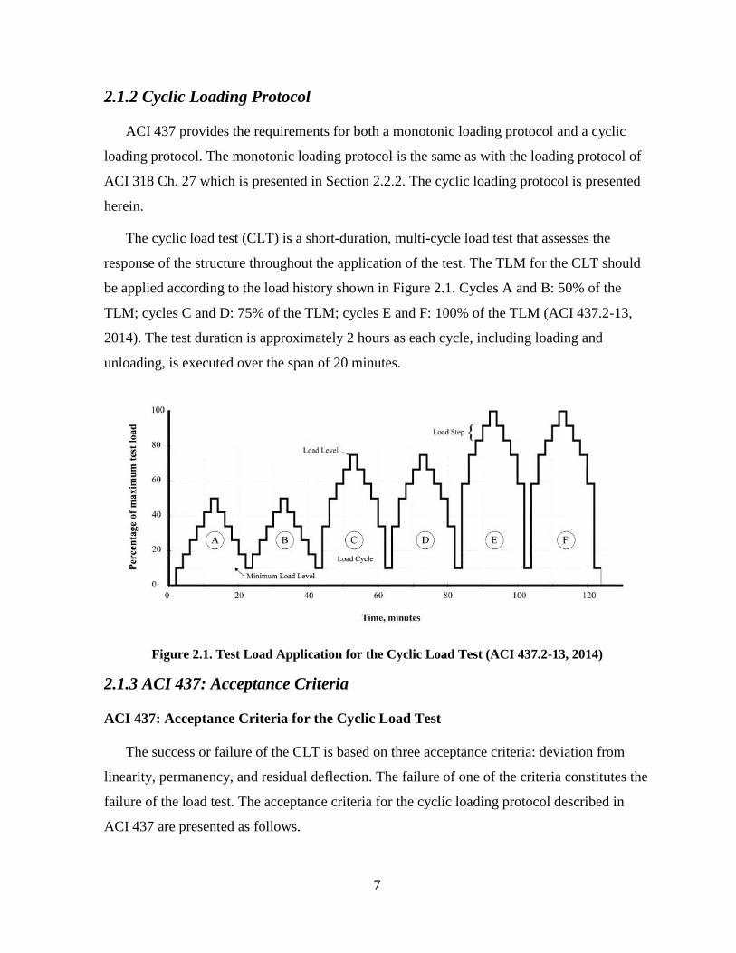
2.1.2 Cyclic Loading Protocol

ACI 437 provides the requirements for both a monotonic loading protocol and a cyclic

loading protocol. The monotonic loading protocol is the same as with the loading protocol of

ACI 318 Ch. 27 which is presented in Section 2.2.2. The cyclic loading protocol is presented

herein.

The cyclic load test (CLT) is a short-duration, multi-cycle load test that assesses the

response of the structure throughout the application of the test. The TLM for the CLT should

be applied according to the load history shown in Figure 2.1. Cycles A and B: 50% of the

TLM; cycles C and D: 75% of the TLM; cycles E and F: 100% of the TLM (ACI 437.2-13,

2014). The test duration is approximately 2 hours as each cycle, including loading and

unloading, is executed over the span of 20 minutes.

Figure 2.1. Test Load Application for the Cyclic Load Test (ACI 437.2-13, 2014)

2.1.3 ACI 437: Acceptance Criteria

ACI 437: Acceptance Criteria for the Cyclic Load Test

The success or failure of the CLT is based on three acceptance criteria: deviation from

linearity, permanency, and residual deflection. The failure of one of the criteria constitutes the

failure of the load test. The acceptance criteria for the cyclic loading protocol described in

ACI 437 are presented as follows.

8

1. Deviation from linearity: is a measure of the nonlinear behavior of the tested member.

Linearity is expressed as the tangent to the slope of two secant lines intersecting the load-

deflection envelope. The reference line is taken at the maximum point in the first cycle

while the other point is taken at any point along the load-deflection envelope that minimizes

linearity. Figure 2.2 presents the load versus deflection schematic of a cyclic load test. A

value of deviation from linearity less than 0.25 indicates a successful outcome of the load

test (ACI 437.2-13, 2014).

𝐼𝐷𝐿 = 𝐷𝑒𝑣𝑖𝑎𝑡𝑖𝑜𝑛 𝑓𝑟𝑜𝑚 𝐿𝑖𝑛𝑒𝑎𝑟𝑖𝑡𝑦 = 1 − tan(𝛼𝑖)

tan(𝛼𝑟𝑒𝑓)

However, ACI 437 Commentary provides a stipulation that states that if a structural section

is uncracked prior to load testing and cracks during the load test, the change in flexural

stiffness due to cracking can cause significant deviations from linearity which would likely

cause this acceptance criterion to fail (ACI 437.2-13, 2014). In such a case, retesting of the

element is permitted as the effects of the uncracked cross section are eliminated in the retest.

Figure 2.2. Schematic of Load vs. Deflection for the Cyclic Load Test (ACI 437.2-13, 2014)

9

2. Permanency: is a measure of the relative value of residual deflection compared to the

corresponding maximum deflection for the second of the two twin loading cycles. This

relationship is illustrated in Figure 2.3. The permanency ratio is considered acceptable if it

does not exceed 0.50 for all load cycle pairs.

𝐼𝑝𝑟 = 𝑝𝑒𝑟𝑚𝑎𝑛𝑒𝑛𝑐𝑦 𝑟𝑎𝑡𝑖𝑜 = 𝐼𝑝(𝑖+1)

𝐼𝑝𝑖

𝐼𝑝𝑖 = ∆𝑟

𝑖

∆𝑚𝑎𝑥𝑖

𝐼𝑝(𝑖+1) = ∆𝑟

(𝑖+1)

∆𝑚𝑎𝑥(𝑖+1)

Figure 2.3. Load-deflection schematic of twin cycles (ACI 437.2-13, 2014)

3. Residual deflection: is the deflection measured 24 hours after the application of the load

test. As residual deflection is measured 24 hours following the removal of the test load,

the total duration of the CLT and post-test evaluation of acceptance criteria is

approximately 26 hours. The residual deflection has to meet the following requirement,

where Δl is the maximum deflection measured during testing (ACI 437.2-13, 2014).

∆𝑟 ≤ ∆𝑙

4

It is important to note that in ACI 437.1R-07 (2007), residual deflection was not considered

as an acceptance criteria for the CLT; however, repeatability was defined as the third

acceptance criterion alongside deviation from linearity and permanency. Repeatability is

briefly described as it is commonly referred to in the CLT application literature between

2005 and 2014.

10

4. Repeatability: is a measure of the response based on the similarity between twin loading

cycles (ACI 437.1R-07, 2007). A repeatability index between 95% - 105% indicates that a

structure or member has passed the load test and is defined as:

𝐼𝑅 = 𝑟𝑒𝑝𝑒𝑎𝑡𝑎𝑏𝑖𝑙𝑖𝑡𝑦 𝑖𝑛𝑑𝑒𝑥 = ∆𝑚𝑎𝑥

𝐵 − ∆𝑟𝐵

∆𝑚𝑎𝑥𝐴 − ∆𝑟

𝐴 × 100%

ACI 437: Acceptance Criteria for the Monotonic Load Test

Under the ACI 437 acceptance criteria for a monotonic loading protocol, a member is

considered to have passed a load test if the test satisfies the following:

∆𝑚𝑎𝑥 ≤ 𝑙𝑡

180

∆𝑟𝑚𝑎𝑥 ≤ ∆𝑚𝑎𝑥

4

If the maximum deflection criteria (∆max) is less than 0.05 in (1.27 mm) or lt/2000, the

residual deflection criterion (∆r max) does not need to be satisfied (ACI 437.2-13, 2014).

2.1.4 ACI 437: Advantages and Disadvantages of the Cyclic Load Test

The CLT was developed to create a novel, reliable testing method to meet the increasing

needs of the structural load testing practice. Some of the advantages of the CLT are:

1. The CLT uses loading and unloading cycles to create a more realistic, real-time assessment

of the performance of an element (Casadei et al., 2005).

2. The CLT acceptance criteria do not only assess maximum deflection but they also assess

the manner in which an element behaves under and recovers from a loading cycle (Casadei

et al., 2005).

3. The overall cost of the CLT has the potential of being lower than the monotonic load test

as the testing duration can be significantly shorter.

4. Although the failure of one of the criteria constitutes the failure of the CLT, the success or

failure of the test is not binary. In the case of failure, practitioners are able to note which

criterion failed and to what degree the failure occurred. Thus, it is possible to make more

educated, diagnostic decisions based on the test results.

11

Although the CLT utilizes modern technology methods, its novelty plays a role in some of

the associated disadvantages.

1. Due to its novelty, there is minimal existing experimental data to provide certainty of

reliability for the CLT. Thus, the TLM, loading protocol, and acceptance criteria may

require calibration as more experimental data becomes available (Galati et al., 2008).

2. Practitioners are likely to recommend either a monotonic or a cyclic load test to building

officials. Thus, in practice, it becomes very unlikely for both tests to be applied and

compared on the same structure. Consequently, it is the responsibility of researchers to

pursue experimental programs that would allow for the comparison of both testing methods

under identical conditions.

2.2 ACI 318-14 Chapter 27

ACI 318-14 is the Building Code Requirements for Structural Concrete; this is the model

code adopted by many building codes in the US and elsewhere. Chapter 27 of ACI 318

(hereafter referred to as ACI 318 Ch. 27) presents code provisions for the strength evaluation

of existing structures through the use of a 24-hour monotonic load test. ACI 318 Ch. 27

Commentary states that a strength evaluation could be performed for various reasons

including, but not limited to:

the quality of materials is considered to be deficient,

there is evidence of faulty or erroneous construction,

there exists noticeable deterioration that may affect structural performance,

if the building is to be repurposed for a new function, or

for any other reasons where the structure does not appear to meet the requirements of the

code (ACI 318-14, 2014).

2.2.1 ACI 318 Ch. 27: Test Load Magnitude

The testing required for the 24-hour monotonic load test (24-h LT) is based on arranging

the TLM to generate maximum, critical deflections over a 24-hour period. The TLM for the

24-h LT should be at least the greatest of (ACI 318-14, 2014):

12

𝑇𝐿𝑀 = 1.3 𝐷

𝑇𝐿𝑀 = 1.15 𝐷 + 1.5 𝐿 + 0.4 (𝐿𝑅 𝑜𝑟 𝑆 𝑜𝑟 𝑅)

𝑇𝐿𝑀 = 1.15 𝐷 + 0.9 𝐿 + 1.5 (𝐿𝑅 𝑜𝑟 𝑆 𝑜𝑟 𝑅)

, where D = dead load; L = live load; LR = roof live load; S = snow load; and R = rain load.

2.2.2 Monotonic Loading Protocol

The TLM is to be applied in not less than four approximately equal increments. Once

100% of the applied test load is achieved, the test load is sustained for 24 hours. Once the 24

hours have passed, the response measurements are made then the load is removed. Then, 24

hours after the test load has been removed, another set of response measurements may be

collected to measure the residual deflection, if necessary. Figure 2.4 illustrates the test load

application of the monotonic load test; the monotonic loading protocol is the same for ACI

437, ACI 318 Ch. 27, and Chapter 20 of CSA A23.3.

Figure 2.4. Test Load Application for the Monotonic Load Test (ACI 437.2-13, 2014)

2.2.3 ACI 318 Ch. 27: Acceptance Criteria for the Monotonic Load Test

The success or failure of the 24-h LT is based on two acceptance criteria. The first

criterion involves visual observation of the tested element; the practitioner must ensure no

excessive cracking, spalling, or deflection is observed during the duration of the test. The

second criterion is a quantitative assessment of the maximum deflection and residual

deflection values after each load increment is applied, after the TLM is sustained for 24 hours,

and 24 hours after the sustained load is removed (ACI 318-14, 2014). Given that the residual

13

deflection is measured 24 hours after the sustained load is removed, the total duration of the

24-h LT is approximately 48 hours. The quantitative criterion considers the maximum

deflection limits satisfying one of the following equations (ACI 318-14, 2014).

∆𝑚𝑎𝑥 ≤ 𝑙𝑡

2

20,000ℎ

∆𝑟𝑚𝑎𝑥 ≤ ∆𝑚𝑎𝑥

4

If the test satisfies the maximum deflection criterion (∆max) then the residual deflection

criterion (∆r max) does not need to be satisfied (Ziehl et al., 2008). Additionally, if the test does

not meet the equations for maximum and residual deflection, it is permitted to repeat the test

72 hours following the completion of the initial test.

2.2.4 ACI 318 Ch. 27: Advantages and Disadvantages of the Monotonic Load Test

The advantages associated with the 24-h LT are:

1. The test uses simple acceptance criteria that are easy to measure, quantify, and assess.

2. Having been in practice for more than 90 years, the 24-h LT is a seemingly reliable method

that has been validated through its application over the period of its existence.

The work of ACI Committee 437 to develop provisions for the CLT included carefully

investigating the validity of the existing 24-h LT. Within that work, the following observations

regarding the 24-h LT were made:

1. Acceptance criteria for the 24-h LT were developed for simply-supported members based

on working stress design limits using material properties and technology available in the

1920s. The acceptance criteria does not provide any flexibility to accommodate for end

fixity or material properties (ACI 437.2-13, 2014).

2. The cost and time associated with the 24-h LT are considerable given that the tested area

has to be cleared and out of service for at least 48 hours, as the residual deflection is

measured 24 hours after the initial 24 hour test is completed (Galati et al., 2008).

3. The result of the 24-h LT is a binary pass-fail as it was designed as a proof load test. The

success of the test only indicates that the member can successfully withstand the TLM; no

additional information beyond that about the ultimate resistance is provided.

14

2.3 CSA A23.3-14

CSA A23.3-14 is the Design of Concrete Structures code provision used in Canada.

Chapter 20 of CSA A23.3-14 (hereafter referred to as CSA A23.3 Ch. 20) presents the code

requirements for load testing of existing structures. The loading protocol used in CSA A23.3

Ch. 20 is a 24-hour monotonic load test similar to that described under Section 2.2.2 for ACI

318 Ch. 27. The advantages and disadvantages of the monotonic loading protocol used in

CSA A.23.3 Ch. 20 is similar to those described under Section 2.2.4 for ACI 318 Ch. 27.

2.3.1 CSA A.23.3 Ch. 20: Test Load Magnitude

The test load shall be equal to 90% of the factored load if the entire structural system is to

be investigated. Otherwise, the test load shall be equal to 100% of the factored load if only one

element is to be investigated (CSA A.23.3-14, 20014).

2.3.2 CSA A.23.3 Ch. 20: Acceptance Criteria

For CSA A23.3, within 24 hours after the removal of the test load, a system or member is

required to have a deflection recovery of 60%, 75%, or 80% based on first test, retest, or

prestressed members, respectively (CSA A.23.3-14, 20014).

2.4 Application of Cyclic and 24-hr Monotonic Load Tests

This section of the literature review provides a review of existing in-situ and experimental

applications for the CLT and 24-hr LT. Table 2.2 summarizes the concepts discussed in each

application paper included in this section. Reinforced concrete (RC) slabs and beams were the

primary type of elements investigated in these studies with one application study investigating

a two-way, post-tensioned slab.

Table 2.2. Concept Summary: Application of 24-h LT and CLT; Ultimate Capacity Margin

Proof Load Testing To Failure

Author (Year) Geometry 24-h LT CLT in-situ FEM UCM

Casadei et al. (2005) RC slab √ √ √ √

Galati et al. (2008) Part 1

Ziehl et al. (2008) Part 2

PT slab

RC slab √ √ √ √

Liu and Ziehl (2009) 14, RC beam

samples √ √ √ √

De Luca et al. (2013) RC slab √ √ √ √

15

2.4.1 In Situ Load Testing of Parking Garage Reinforced Concrete Slabs:

Comparison between 24 h and Cyclic Load Testing

Casadei et al. (2005) use in-situ application of both the CLT and the 24-hr LT on a

parking garage with one-way reinforced concrete slabs. This is one of the earliest application

papers reporting on the comparison between the CLT and the 24-hr LT. The tests were

conducted on identical slabs in the parking structure.

It was determined that both slabs did not pass each respective load test which showcased a

consistent outcome regardless of load testing protocol. For this specific case study, the CLT

and 24-hr LT yielded the same final outcome considering slabs that were subjected to the

same test load magnitude.

Since the structure was scheduled for demolition, the slabs were loaded to failure

following each load test. This allowed for the calculation of the Ultimate Collapse or Ultimate

Capacity Margin (UCM) to be determined as per the following equation:

𝑈𝐶𝑀(%) = ( 1 − 𝑃𝑡𝑒𝑠𝑡−𝑙𝑜𝑎𝑑

𝑃𝑢𝑙𝑡−𝑓𝑎𝑖𝑙𝑢𝑟𝑒 ) × 100%

; where, Ptest-load is the load at which the structure exceeded an acceptance criterion and Pult-

failure is the load at which the structure was deemed to have reached its ultimate capacity.

It was determined that the remaining strength reserve of the system beyond the test load

magnitude was 18% for the CLT and 20% for the 24-hr LT. The similarity of the outcome

between the CLT and 24-hr LT showcased promise that there is a likelihood of consistency

between the two load tests. It was demonstrated that quantifying the UCM may provide

greater insight into the resistance of a structure beyond proof loading which may be helpful to

stakeholders and practitioners (Casadei et al., 2005).

2.4.2 In-Situ Evaluation of Concrete Slab Systems

This two-part research paper focused on conducting the CLT and the 24-hr LT in two

experimental scenarios: a two-way post-tensioned (PT) concrete slab system and a two-way

reinforced concrete (RC) slab system. The two-way PT concrete slab was investigated as it

was believed that the system was inadequate in both flexure and shear resistance due to many

16

areas being characterized by tendon and reinforcement misplacement. The two-way RC slab

system was investigated as the system exhibited distributed cracking at the positive and

negative moment regions (Galati et al., 2008).

Using commercial Finite Element (FE) software, SAP 2000, the maximum theoretical

deflection was generated in comparison to the maximum experimental deflection collected on

site. Using uncracked and cracked assumptions in the FE model and comparing to the

experimental results, it was evident that the first two CLT cycles exhibited uncracked

behavior and the last two CLT cycles exhibited cracked behavior. The two middle CLT cycles

exhibited uncracked behavior in the two-way post-tensioned concrete slab and cracked

behavior in the two-way RC concrete slab. The outcomes of the CLT acceptance criteria are

highly sensitive to the status of the section, whether cracked or uncracked, prior to load

testing (Galati et al., 2008).

In Part II of this paper, the use of Acoustic Emission (AE) in both experimental

procedures was discussed. Ziehl et al. state that AE used in conjunction with CLT creates

more informative, complimentary testing outcomes. The acceptance criteria used to assess the

structures in this research are presented in Table 2.3 (2008).

Table 2.3. Acceptance Criteria Proposed by Ziehl et al. (2008)

CLT 24-Hour Load Test AE

Repeatability Maximum Deflection Calm Ratio vs. Load Ratio

Permanency Residual Deflection Cumulative Signal Strength Ratio

Deviation from Linearity

The two-way PT concrete slab was deemed satisfactory under both the CLT and the 24-hr

LT with AE results confirming cracking and deflection phenomena throughout testing. Only

CLT and AE experimentation was conducted for the two-way RC slab. Under the CLT, the

slab failed the permanency and deviation from linearity criteria at load set 3 and beyond.

Under AE, the slab exceeded the Cumulative Signal Strength Ratio limit at load set 4 and

beyond.

As both experimental structures were still in service, the slabs were not taken to failure.

However, the UCM was obtained using the calibrated FE model which was developed

17

previously to estimate deflections. Ptest-load was the load at which an acceptance criteria failed

while Pult._failure was the theoretical ultimate load or moment capacity of the slab. The UCM for

each acceptance criteria was calculated based on the findings from the FE model; UCM

results ranged from 19 – 33% with one data set at 54%. UCM values of 19 – 33% from the FE

model were comparable to the UCM values of 18% and 20% from the experimental results

presented by Casadei et al (2005).

2.4.3 Evaluation of Reinforced Concrete Beam Specimens with Acoustic

Emission and Cyclic Load Test Methods

This paper presents CLT and AE results applied to 14 controlled, RC beam specimens in a

laboratory environment. It is important to note that the samples used in this research were

reduced-scale (152 x 152 x 762 mm) samples. Three dimensional, nonlinear FE models were

created to establish the ultimate load of each specimen.

The cyclic loading protocol used in this research included additional cycles compared to

the cyclic loading protocol proposed in ACI 437. Furthermore, the Simplified CLT (SCLT)

was used on some samples. The SCLT involved using the same loading schematic as the CLT

while applying continuous loading and unloading cycles instead of discrete incremental cycles

as illustrated in Figure 2.5.

Figure 2.5. Schematic of the CLT versus the SCLT Loading and Unloading Pattern

(Liu & Ziehl, 2009)

The experiment was designed using the breakdown presented in Table 2.4. The number in

the bracket indicated the number of samples tested using that experiment.

18

Table 2.4. Liu and Ziehl Experimental Study Summary (2009)

Failure Mode Concrete Type Load Pattern

Flexure

Conventional (5) CLT (5)

Self-consolidating (4) CLT (2)

SCLT (2)

Shear

Conventional (2) CLT (2)

Self-consolidating (3) CLT (2)

SCLT (1)

The following findings were observed for samples tested under flexure and samples tested

under shear:

The deviation from linearity criterion is usually exceeded if the initially uncracked

condition is assumed; however, when the cracked condition is assumed, this criterion was

the most sensitive to the degree of damage of the specimen (Liu & Ziehl, 2009).

There was no difference in the evaluation results attributed to CLT and SCLT or

conventional and self-consolidating concrete.

Similar to previous research, the UCM was calculated for the CLT acceptance criteria. In

this case, Pult-failure is the experimentally defined ultimate load capacity. The research

primarily focused on the effects of AE acceptance criteria on the UCM.

2.4.4 Assessment of Performance of Reinforced Concrete Strips by In-Place

Load Testing

The experimental site utilized in De Luca et al. (2013) is a three-story apartment building

which was scheduled for demolition. Two identical strips of one-way RC slabs were tested

under the CLT and the 24-hr LT.

The two slabs were tested under the CLT followed by the monotonic 24-hr LT; then, both

tests were repeated (total of 4 load tests per slab strip). After all testing was conducted, both

slabs were taken to failure; failure was defined by the midspan deflection exceeding 1/100 of

the clear span. The two slabs presented similar behavior under each load test; however, one of

the slabs was slightly stiffer and experienced less permanent changes than the other. This

difference is possibly attributed to the type of service condition that each slab experienced

19

during its service life (De_Luca_et_al.,_2013). Additionally, consideration was given to the

type and ideality of support conditions present in each case.

Both slab assemblies initially failed the first CLT, based on the deviation from linearity

criterion, but passed the second test; it was determined that this was likely due to the sections

being in an uncracked state prior to load testing. The 24-hr LT does not seem to add any

supplementary valuable information beyond what is concluded through the CLT.

The findings from this study were inconsistent with UCM outcomes identified in previous

studies. After the second test, where the slab passed the load test once the section was

cracked, the TLM based on ACI 437-12 was approximately one quarter of the ultimate load.

Although the UCM was not explicitly calculated in this research, the TLMeq was 1,600 lbs

while the Failure Load was 9,400 lbs. That constitutes a UCM of ~83% which is significantly

higher than previously defined UCM values generally in the 18% to 30% range.

2.5 Reliability-Based Design

The first step to understanding the reliability assessment of load testing is to gain an

understanding of the reliability-based calibration of design codes. Design reliability is a

method to probabilistically assess the resistance and load effects acting on a structural

element. Assuming the resistance of an element, R, and load effects acting on the element, S,

are random variables, the limit state results in the inequality:

Probability of Failure: Pf = P[R ≤ S]

Considering the failure domain where the set of couples of (r,s) exist, the probability of

failure for a typical design case can be assessed using Equation 1 (Cremona, 2011)..

𝑃𝑓 = 𝑃[𝑆 > 𝑅]

= ∫ 𝑃[𝑆 > 𝑅 = 𝑟 | 𝑅 = 𝑟] 𝑃[𝑅 = 𝑟]

= ∫ 𝑃[𝑆 > 𝑟] 𝑓𝑅(𝑟) 𝑑𝑟∞

0

= ∫ [1 − 𝐹𝑆(𝑟)] 𝑓𝑅(𝑟) 𝑑𝑟∞

0

𝑃𝑓 = 1 − ∫ 𝐹𝑆(𝑟) 𝑓𝑅(𝑟) 𝑑𝑟∞

0

− − − − − − − − − − − − − − − − − − − [𝐸𝑞𝑢𝑎𝑡𝑖𝑜𝑛 1]

20

2.5.1 Normal Random Variables

Where both R and S are assumed to have normal distributions, the process of computing

the reliability index, β, and the probability of failure, Pf, is expedited. Since the difference

between two normal variables is a normal variable, the difference between R and S can be

defined by the normal variable Z; such that μZ = μR – μS and σ2Z = σ

2R – σ

2S (Cremona, 2011).

The shaded area in Figure 2.6 (A) represents the probability of failure region where the load

effect exceeds the resistance of an element

(A) (B)

Figure 2.6. Probability of Failure (A) and Reliability Index (B)

The reliability index, β, and the probability of failure, Pf, are defined by:

𝑃𝑓 = 𝑃[𝑅 − 𝑆 ≤ 0] = 𝑃[𝑍 ≤ 0]

𝛽 = 𝜇𝑅 − 𝜇𝑆

√𝜎𝑅2 + 𝜎𝑆

2 − − − − − − − − − − − − − − − [𝐸𝑞𝑢𝑎𝑡𝑖𝑜𝑛 2. 𝑎]

𝑃𝑓 ≈ Φ (−𝛽) − − − − − − − − − − − − − − − − − [𝐸𝑞𝑢𝑎𝑡𝑖𝑜𝑛 2. 𝑏]

, where μi = mean of i; σi = standard deviation of i; and Φ = standard normal density function.

The reliability index, β, expresses the relationship of standard deviation between Z and 0.

As β increases, the level of required safety increases; therefore, the probability of failure

decreases. As can be seen in Figure 2.6 (A), β σZ is equal to the difference between the µR and

µS (the numerator of the β equation). As can be seen in Figure 2.6 (B), β σZ is equal to the

difference between µZ and 0 in the Z distribution.

21

Table 2.5 showcases the relationship between the reliability index, β, and the probability

of failure, Pf. It is important to note that β must be taken to at least two significant figures as

the value and order of magnitude of Pf is highly sensitive to the value of β (Cremona, 2011).

Table 2.5. Reliability Index and Probability of Failure (Cremona, 2011)

β 0.0 1.28 2.33 3.09 3.72 4.26 4.75 5.20

Pf 5 10-1 10-1 10-2 10-3 10-4 10-5 10-6 10-7

2.6 Reliability-Based Calibration of Design Code for Buildings

A two-part technical paper was presented by Nowak and Szerszen (2003) summarizing

the process used in the calibration of ACI 318 following the adoption of loads and load

combinations from ASCE 7, Standard on Minimum Design Loads for Buildings and Other

Structures, in 2002. Understanding the reliability-based calibration process is the foundation

of the reliability-based load testing assessment.

2.6.1 Calibration Procedure

The selection of resistance factors for different structural types and limit states is based on

the following calibration process. The goal of the calibration procedure is to identify the most

probable range of reliability indices that a structural type experiences based on its resistance

properties and loading parameters.

1. Element Selection: the types of structural elements and materials covered by ACI 318 are

identified. The most representative dimensions and reinforcement ratios for structural

elements are selected and modeled over load component values of D/(D+L), where D =

dead load and L = live load.

2. Statistical Load Model: using the database of load parameters available in the literature,

statistical models of load components are developed based on Turkstra’s Rule. Turkstra

observed that only one load component experiences its extreme value while others are at

their corresponding average values (Nowak & Szerszen, 2003).

3. Resistance Model Selection: resistance properties are defined by the statistical

parameters of the material, fabrication, and professional design. This is done by reviewing

existing databases of material properties or collecting new data.

22

4. Reliability Analysis: based on the resistance model and load model for each structural

element and failure mode, the reliability index is measured to investigate levels of safety

across all D/(D+L) values.

Statistical Parameters of Load Combinations:

The statistical parameters of load combinations from literature are summarized in Table

2.6. The dead load is time invariant; therefore, it is the same for both the arbitrary point-in-

time load and the maximum 50-year load. ACI 318 includes load combinations using dead,

live, snow, wind, and earthquake loads. As demonstrated in Szerszen & Nowak (2003), and

used hereafter in this research, reliability-based calibration utilizes the basic load combination

of D_+_L; the load models presented in Szerszen & Nowak (2003) are normally distributed.

Table 2.6. Statistical Parameters of Load Combinations (Szerszen & Nowak, 2003)

Load Component Arbitrary Point-in-time Load Maximum 50-year Load

Bias COV Bias COV

Dead load (cast-in-place) 1.05 0.10 1.05 0.10

Dead load (plant-cast) 1.03 0.08 1.03 0.08

Live Load 0.24 0.65 1.00 0.18

Snow 0.20 0.87 0.82 0.26

The mean and standard deviation of the total load distribution are calculated by summing

the components from the governing load combination using Turkstra’s Rule. Turkstra’s Rule

observed that the maximum value of a load combination is attributed to the occurrence of the

maximum value of one of its components; for example, if a dead, live, and snow load

combination (D_+_L_+_S) was considered, the maximum value of that load combination

would occur when either the live load or the snow load is at its maximum 50-year load while

the other is at the arbitrary point-in-time load.

Statistical Parameters of Resistance:

The resistance model is the combination of three factors: material properties parameter,

fabrication properties parameter, and the professional factor. As resistance modelling is a

major component of this research, relevant outlines of resistance modelling are provided

within each chapter of this thesis as needed.

23

2.7 Structural Load Testing Reliability: Conditional Probability

In probability theory, conditional probability is defined as the probability of an occurrence

of an event given that another has already occurred. In load testing, conditional probability

will revise and enhance the estimate of reliability of an element assuming that the element has

withstood the test load. Figure 2.7 (B) illustrates the manner in which the existing resistance

probability distribution, fR, changes to the truncated probability distribution, f’R, after the

proof load, q*, is applied (Hall, 1988). This can be described by conditional probability theory

using the following equations:

𝑓𝑅′(𝑟) =

𝑓𝑅 (𝑟)

1 − 𝐹𝑅 (𝑞∗) 𝑟 ≥ 𝑞∗ − − − − − − − − − − − − − − − [𝐸𝑞𝑢𝑎𝑡𝑖𝑜𝑛 3. 𝑎]

𝑓𝑅′(𝑟) = 0 𝑟 < 𝑞∗ − − − − − − − − − − − − − − − [𝐸𝑞𝑢𝑎𝑡𝑖𝑜𝑛 3. 𝑏]

(A) (B)

Figure 2.7. Probability of Failure Regions before (A) and after (B) the application of a load test

The probability of failure, Pf, is defined as the intersection of the load effects, fS, and

resistance, fR, probability distributions. Once the proof load is applied, the updated resistance,

f’R, has a smaller intersection with fS, thus has a lower probability of failure. A successful

proof load test statistically confirms that the possibility of erroneously constructed, low-

strength members is non-existent in the tested scenario up to the test load level, q*.

Therefore, to calculate the probability of failure after proof load testing, the probability of

failure can be updated by substituting f’R (r) from Equation 3 in place of fR (r) in Equation 1.

In addition, the lower integral limit defining Pf becomes equal to the TLM, q*. This yields:

24

𝑃𝑓 = 1 − ∫ 𝐹𝑆(𝑟) 𝑓𝑅′′(𝑟) 𝑑𝑟

∞

𝑞∗

= 1 − ∫𝐹𝑆(𝑟) 𝑓𝑅(𝑟)

1 − 𝐹𝑅(𝑞∗) 𝑑𝑟

∞

𝑞∗

= 1 − 1

1 − 𝐹𝑅(𝑞∗) ∫ 𝐹𝑆(𝑟) 𝑓𝑅(𝑟) 𝑑𝑟

∞

𝑞∗

− − − − − − − − − − − − − [𝐸𝑞𝑢𝑎𝑡𝑖𝑜𝑛 4]

2.7.1 Reliability-based Approaches to Load Testing

Stewart (1997) uses concepts presented in Hall’s research (1988) to develop probabilistic

models of structural reliability based on proof load testing, inspections, and gross error. The

research uses resistance and load parameter variability to develop Monte Carlo Simulations for

a single case study. Stewart provides clear steps to complete the computational procedure to

calculate the probability of failure by modelling resistance and load probability distributions

based on parameter variability using Monte Carlo simulations. The concepts of model error,

construction error, human reliability analysis, and service proven structures are incorporated

into the probabilistic resistance and load models.

2.8 Load Testing in Bridge Evaluation: AASHTO MBE

Concepts of load testing in the evaluation of bridges are similar to those of structures;

however, load testing in bridge evaluation provides practitioners with additional flexibility in

the assessment of an existing bridge. Chapter 8 of the American Association of State Highway

and Transportation Officials (AASHTO) The Manual for Bridge Evaluation (MBE) includes

the provisions for nondestructive load testing of bridges.

AASTHO MBE prescribes an adjustable test load magnitude live load factor depending

on several considerations; this is quite different from the fixed test load magnitudes associated

with load testing for building evaluation prescribed by ACI 437 and ACI 318 Ch. 27. Table

2.7 presents the considerations for the adjustment of the test load magnitude live load factor.

The MBE states that these “should be considered as minimum values; larger values may be

selected by the Engineer as deemed appropriate” (AASHTO, 2014).

25

Table 2.7. Test Load Magnitude Live Load Factor Adjustments for Bridge Evaluation

(AASHTO, 2014)

Consideration Adjustment

One-Lane Load Controls +15%

Nonredundant Structure +10%

Facture-Critical Details Present +10%

Bridges in Poor Condition +10%

In-Depth Inspection Performed -5%

Rateable, Existing RF > 1.0 - 5%

ADTT < 1000 -10%

ADTT < 100 - 15%

Appendix A of this thesis includes a literature review of reliability-based assessment of

bridges using structural load testing. Most notably, Faber et al. (2000) developed complex

models proposing variable proof load magnitudes based on the age of the bridge at the time of

load testing to achieve a desired rating.

26

Chapter 3 Reliability Assessment of Test Load

Magnitudes: ACI 437 and ACI 318 Ch. 27

To develop the fundamentals of reliability-based load testing, the foundations of structural

design calibration and target reliability levels were reviewed. Once the code calibration

models were recreated, a conditional probability algorithm was developed and applied using

MATLAB to demonstrate the post-load testing reliability of an element. The test load

magnitudes (TLM) used within the conditional probability algorithm were based on the TLMs

of ACI 437 and ACI 318 Ch. 27.

Once the as-designed post-load testing model was examined, the effects of assumed

deterioration (reduced strength) or occupancy change (increased live load) on post-load

testing reliability were considered. These two cases were considered as they were deemed to

be common situations in the evaluation of an existing structure.


Target reliability levels are not explicitly or quantitatively defined for the cyclic load test

(CLT) or the 24-hour monotonic load test (24-h LT) prescribed by ACI 437 and ACI 318 Ch.

27, respectively. Therefore, the current qualitative pass-or-fail outcome based on the

acceptance criteria of each code may not provide indication of a consistent, quantitative level

of post-load testing reliability, typically defined by the reliability index, β, or probability of

failure, Pf. The test load magnitude (TLM) and loading protocols are different for each of the

load tests; thus, the current qualitative reliability verification achieved by performing a load

test is expected to be quantitatively inconsistent between each of the two load tests.

A further consideration is that a successful load test satisfying the acceptance criteria

implies that the element or structure is adequate for the design loads and corresponding TLM

as specified in the governing Code. However, since the post-load testing reliability index (or

probability of failure) is not known, the underlying post-load testing reliability with respect to

the target design reliability levels used in the calibration of ACI 318 is also not known.

27

3.2 Research Objective

The primary objective of the reliability assessment described in this chapter is to provide

insight into the reliability of a structural element or system as indicated by proof load test. The

specific objectives are:

To establish the post-load testing reliability associated with each of the TLMs presented in

ACI 437.2-13 and ACI 318 Ch. 27 using conditional probability.

To compare the post-load test reliability levels with target design reliability of a reinforced

concrete (RC) element designed according to ACI 318-14.

Demonstrate the effects of assumed deterioration (reduced strength) or occupancy change

(increased live load) on the post-load testing reliability in scenarios where load testing

may be applied.

The reliability analyses in this chapter are limited to assessing the differences between the

TLM of ACI 437 and ACI 318 Ch. 27 and are based on the assumption that the tested element

or structure passed the load test by meeting the specified acceptance criteria; the mechanistic

difference in load protocols and acceptance criteria between the tests is not quantitatively

investigated in this research.

The target reliability indices and statistical parameters as used in the calibration of ACI

318 were obtained from Nowak & Szerszen (2003). Furthermore, updated parameters for

certain statistical parameters of resistance were obtained from Nowak et al. (2012).

3.3 Background for Reliability Analysis

3.3.1 Test Load Magnitudes

Table 3.1 summarizes the TLM for ACI 437 (Case I and Case II) and ACI 318 Ch. 27.

Probabilistically, the TLM is considered to be the load level, q*, at which the resistance

probability density function is truncated. The most noticeable differences between the TLM

for ACI 437 and ACI 318 Ch. 27 are the difference in the live load factor and the separation,

or amalgamation, of dead load components. The live load factors constituting the TLMs can

be arranged from lowest to highest in the following order: ACI 437 Case II (αL = 1.40), ACI

318 Ch. 27 (αL = 1.50), and ACI 437 Case I (αL = 1.60). It can be conceived that ACI 437

28

made a distinction between Case I and Case II as upper and lower bounds while the TLM for

ACI 318 Ch. 27 falls in the middle of that range of live load factors.

Table 3.1. Test Load Magnitudes for ACI 437 and ACI_318_Chapter 27

Code Provision Test Load Magnitude – not to be less than the largest of:

ACI 437 Case I TLM = 1.3 ( DW + DS )



; only part of the portions of a structure that are suspected of

containing deficiencies are to be load tested and members to be

tested are statically indeterminate.

ACI 437 Case II TLM = 1.2 ( DW + DS )


TLM = 1.0 DW +1.1 DS + 0.9 L+1.4 (LR or S or R)

; all suspect portions of a structure are to be load tested or when

the elements to be tested are determinate and the suspected flaw

is controlled by flexure.

ACI 318 Ch. 27 TLM = 1.3 D

TLM = 1.15 D +1.5 L+0.4 (LR or S or R)

TLM = 1.15 D +0.9 L+1.5 (LR or S or R)

where: D = dead load; Dw = dead load due to self-weight; Ds = superimposed dead load; L

= live load; LR = roof live load; S = snow load; and R = rain load.

ACI 437 makes the distinction between the dead load due to self-weight (αDw = 1.0) and

the dead load due to superimposed dead load (αDs = 1.1) while ACI 318 Ch. 27 combined both

dead load components into a single, larger factor (αD = 1.15). ACI 437 states that the reason

dead load separation is implemented is due to the notion that a proof load should be defined in

terms of the components of the load that are likely subject to variability; therefore, given that

the dead load due to self-weight is not subject to variability, its factor should be equal to 1.0

(ACI 437.1R-07, 2007).

3.3.3 Statistical Parameters of Resistance for Beams and Slabs

To characterize the resistance distribution in the processes of defining the reliability of an

element, Nowak et al. (2012) derived the statistical parameters (bias and COV) of resistance

for different element types and failure modes. The statistical parameters of the resistance

distribution are dependent on the variability of the material and fabrication properties (f’c, fy,

29

As, d, b) that are inputs of the moment resistance equation. Note that the statistical parameters

of each of the material and fabrication properties are detailed in Section_4.3.

𝑹 = 𝑨𝒔 𝒇𝒚 (𝒅 −𝒂

2) [𝐸𝑞𝑢𝑎𝑡𝑖𝑜𝑛 5. 𝑎]

where,

𝒂 =𝑨𝒔 𝒇𝒚

0.85 𝒇𝒄′ 𝒃

[𝐸𝑞𝑢𝑎𝑡𝑖𝑜𝑛 5. 𝑏]

The statistical properties of resistance, R, for an RC beam and RC slab are presented in

Table 3.2. The resistance models utilized by Nowak et al. (2012) are assumed to have a

normal distribution.

Table 3.2. Statistical Parameters of Resistance for RC Beam and RC Slab (Nowak et al., 2012)

Structural Type Design Case Bias Factor, λ Coefficient of Variation, COV

RC Beam, flexure ρ = 0.6% 1.140 0.080

RC Beam, flexure ρ = 1.6% 1.130 0.085

RC Slab, flexure ρ = 0.3% 1.055 0.145

The statistical parameters of resistance were developed through conducting Monte Carlo

simulations (Nowak & Szerszen, 2003). The bold values in the equation for bending

resistance of flexural members (Equation 5) represent values that are variable in each iteration

of the Monte Carlo simulation. Note that the element width, b, is variable for beam elements

but is constant (1 m width) for slab segments.

Monte Carlo Simulation

Monte Carlo simulation is a rigorous method of reproducing real world problems using

hypotheses and models to determine the probability of failure of a system. For each trial, a

random variable is generated based on the statistical properties of each parameter. This is

conducted repeatedly for a predetermined number of trials. Then, taking into consideration the

limit state function, Pf can be calculated by dividing the number of times the simulation

exceeded the limit state functions by the total number of simulations (Cremona, 2011).

30

For a single iteration of the Monte Carlo simulation for the resistance, R, single values of

f’c, fy, As, d, and b were generated; these values are different in each iteration based on the

statistical parameters of each material and fabrication property (summarized in Section 4.3).

Then, the material and fabrication properties were combined using the equation for bending

resistance for flexural members (Equation 5) to generate a single value of resistance, R.

Finally, R is adjusted by the professional factor, P. The recommended bias for P is 1.02

while the recommended COV for P is 0.06 (Ellingwood et al., 1980). Therefore, for a single

iteration of the Monte Carlo simulation, a P factor was generated. The P factor was generated

by calculating the inverse of the normal cumulative distribution with a mean 1.02 and

standard deviation = 0.06 at a randomly generated value between 0 and 1 (which acts as the

randomly generated probability). Then, R is multiplied by P and thus accommodating for the

variability in analysis and testing methods associated with obtaining R. To determine the final

statistical parameter of resistance, this single iteration of R was repeated by a specified

number of iterations, N.

3.4 Procedure Overview

To examine the reliability of a structural element after load testing using ACI 437 and

ACI 318 Ch. 27, the probability of failure was used as the quantitative reliability parameter.

The target Pf was used as a reference benchmark in comparison to the post-load test Pf.

MATLAB was used to facilitate the computation of numerical integrals and create the

visualizations presented hereafter; the base MATLAB function is provided in Appendix B. An

overview of the procedure used to conduct this reliability assessment is outlined in Figure 3.1.

Figure 3.1. Procedure Flowchart

1. Case Selection: to provide a holistic representation of various occupancy scenarios, data

was plotted along a scale of D/(D+L) from 0 to 1, where D = dead load effect and L = live

1. Case Selection

2. Baseline Design

Reliability

3. Load Testing Reliability

4. & 5. Effects of Deterioration

and Occupancy Change

31

load effect. The structural elements selected for investigation were cast-in-place, RC

beams and cast-in-place, RC slabs.

2. Design Reliability: for cast-in-place, RC beams and cast-in-place RC slabs governed by

flexural failure, using statistical parameters for load components and resistance models,

the design Pf was established as a representative target or benchmark. The detailed

procedure to establish design reliability is outlined under Section 2.5 and 2.6. The as-

designed (target) β and Pf are shown below. The equation for β assumes that both the

resistance and load distributions are normally distributed.



2 [𝐸𝑞𝑢𝑎𝑡𝑖𝑜𝑛 2. 𝑎] 𝑃𝑓 ≈ Φ(−𝛽) [𝐸𝑞𝑢𝑎𝑡𝑖𝑜𝑛 2. 𝑏]

To calculate the mean and standard deviation of resistance to be used in the equation for β,

the design resistance, R, and the resistance statistical parameters (bias and COV from

Table 3.2) must be defined. Additionally, the element strength reduction factor, ϕ = 0.9 for

both beams and slabs, must be identified as per the Code (ACI 318-14, 2014).

For a cast-in-place, RC beam, the bias and COV values are 1.140 and 0.080, respectively

(from Table 3.2). Assuming a design resistance, Rdesign, equal to 129 kN-m, the mean, μR,

and standard deviation, σR, are equal to:

𝜇𝑅 = 𝑅𝑛 × 𝑏𝑖𝑎𝑠𝑅 𝜇𝑅 = 129

0.9 × 1.140 = 163.4 𝑘𝑁𝑚

𝜎𝑅 = 𝜇𝑅 × 𝐶𝑂𝑉𝑅 𝜎𝑅 = 163.4 𝑘𝑁𝑚 × 0.080 = 13.07

where, the nominal resistance, 𝑅𝑛 = 𝑅𝑑𝑒𝑠𝑖𝑔𝑛

𝜙.

Similarly, the mean, μS, and standard deviation, σS, of the load effects distribution, S, can

be evaluated using the statistical parameters of load combinations presented in Table 2.6.

3. Load Testing Reliability - Test Load Magnitude: using the concepts of conditional

probability and proof load testing (from Section 2.7), the TLM was applied, according to

TLMs prescribed in ACI 437 and ACI 318, over all D/(D+L) values. Then, the updated Pf

values were computed for each D/(D+L) and compared to the design Pf.

32

𝑃𝑓 = 1 − 1


∞

𝑞∗

− − − − − − − − − − − [𝐸𝑞𝑢𝑎𝑡𝑖𝑜𝑛 4]

; where, q* is the TLM at each D/(D+L) value based on the prescribed code.

Appendix B includes the base MATLAB code used to compute this integral through

trapezoidal numerical integration. For a given TLM, q*, defined through ACI 437 or ACI

318, at a given D/(D+L) ratio:

a. Increments, i, between q* and ∞ were created at 0.001 increments. The value of ∞ was

taken as a value that is sufficiently greater than q*. Various discretization increments

were considered; 0.001 was selected as it provided accurate and smooth graphical

output while allowing the MATLAB code to compute within a reasonable time.

b. For each increment, i, the interior of the integral was computed. The load normal

cumulative distribution, FS, computed at i is multiplied by the resistance normal

probability density distribution, fR, computed at i. As the upper bound of the integral

increases, the computation of the interior of the integral approaches zero (thus, ∞ was

selected at a value, sufficiently greater than q*, where this condition is satisfied).

c. Now, the integral was computed through trapezoidal numerical integration, by

integrating the output of 3.b. by the increments from 3.a.

d. The coefficient outside the integral was calculated; the resistance normal cumulative

distribution, FR, (with a μR and σR) was calculated at each i to compute FR (q*).

e. Finally, Pf is computed by multiplying the resulting coefficient (3.d.) with the integral

(3.c.). This Pf represents the post-load testing Pf of the investigated TLM, q*, based on

ACI 437 or ACI 318 at a single D/(D+L) increment. These steps are repeated at each

D/(D+L) increment.

For the ACI 437 TLM, the model assumed that the dead load component is divided

equally between the self-weight, Dw, and the superimposed dead load, Ds.

4. Effects of Deterioration: by postulating incremental deterioration levels, the reliability

effects of each load test were investigated over all D/(D+L) values. Deterioration was

defined as the percentage transformation to the mean of the R distribution; it was assumed

that the change in the mean of R does not cause a change in the COV. Then, the updated

33

values of μR and σR were used in Step 2 and Step 3 to calculate the deteriorated β and the

post-load testing Pf for the deteriorated element.

5. Effects of Occupancy Change: by postulating incremental occupancy (live load) change

levels, the reliability effects of each load test were investigated over all D/(D+L) values.

Occupancy change was defined as the percentage transformation to the mean of the live

load which in turn transforms the S distribution. The updated values of μS and σS were

used in Step 2 and Step 3 to calculate the updated β and the post-load testing Pf for the

element being investigated for a proposed occupancy change.

By observing how Pf varies for each load test in each of these analyses, a reliability-based

understanding of load testing was achieved.

3.5 Reliability Assessment Results

To ensure that the baseline reliability was calibrated to data generated by Szerszen &

Nowak (2003), a baseline β model was developed in MATLAB. This initial step was

conducted using data from Szerszen & Nowak (2003) as their research included clear

graphical output. However, once the MATLAB model was deemed to be an accurate

reflection of the Szerszen & Nowak (2003) output, the updated resistance statistical

parameters from Nowak et al. (2012) were used in the MATLAB model. The goal of using

the Nowak et al. data for this research was to reflect the most up-to-date statistical parameters

of resistance available in the literature.

As illustrated in Figure 3.2 and Figure 3.3, the reliability index model developed by

Szerszen & Nowak (2003) was accurately recreated in the MATLAB model developed for

this research. For the cast-in-place, RC beam models in Figure 3.2, this was verified by

comparing key points on the original and MATLAB models; β was equal to 4.25, 4.0, and 3.5

at D/(D+L) values of 0, 0.65, and 0.88, respectively. For the cast-in-place, RC slab models in

Figure 3.3, this was verified by comparing key points on the original and MATLAB models; β

was equal to 2.75, 2.5, and 2.0 at D/(D+L) values of 0, 0.55, and 0.80, respectively.

For cast-in-place, RC beams governed by flexural failure, Figure 3.2 showcases the

reliability index associated with the design case at an element resistance factor, ϕ, of 0.9. The

resistance factor, ϕ, is determined for each structural type and limit state through calibration

34

so that “the reliability of designed elements is consistent with a predetermined target level”

(Szerszen & Nowak, 2003). Although D/(D+L) values were presented from 0 to 1, the most

probable D/(D+L) values for beams are from 0.3 to 0.7 (Szerszen & Nowak, 2003). For cast-

in-place, RC slabs governed by flexural failure, Figure 3.3 showcases the reliability index

associated with the design case at a resistance factor, ϕ, of 0.9. The most probable D/(D+L)

values for slabs are from 0.3 to 0.6 (Szerszen & Nowak, 2003).

For the design case β model for cast-in-place, RC beam and cast-in-place, RC slab, β

values were plotted for the load combination of αD D + αL L from D/(D+L) values of 0 to

0.88; beyond that, the load combination of αD D dominated. Therefore, the point of inflection

in the reliability index over the range of D/(D+L) values was caused by a change in the

governing load combination.

It is evident that the reliability of a cast-in-place, RC beam is different from a cast-in-

place, RC slab. There is inherent uncertainty in the effective depth of an element, especially

for cast-in-place construction. Given that the member resistance is highly sensitive to the

effective depth, even a small change in the effective depth can have a large impact on the

reliability index. This phenomena is more significant in slabs as the effective depth tends to

be small relative to the effective depth of a beam; thus, any small change in the effective

depth has a more drastic effect on the slab resistance (Szerszen & Nowak, 2003).

Figure 3.3 showcases the reliability for a slab with a 1 ft (or 1m) unit width. From a

reliability-based standpoint, a slab assembly is designed as a parallel system of combined

elements of unit widths. Thus, the overall reliability of a slab system is significantly higher

than the reliability of each individual unit width slab strip and, in many cases, may be similar

to or larger than the reliability of a beam (Szerszen & Nowak, 2003).

35

Figure 3.2. Left: RC Beam β Model (Szerszen & Nowak, 2003); Right: Recreated β MATLAB

Model

Figure 3.3. Left: RC Slab β Model (Szerszen & Nowak, 2003); Right: Recreated β MATLAB

Model

36

The baseline data from statistical parameters for beams and slabs was based on a

predetermined reinforcement ratio, ρ. The resistance models for beams were investigated

based on ρ = 0.6% and 1.6% while slabs were investigated based on ρ = 0.3%. These ratios

are based on most probable bounds identified by ACI 318 (Nowak et al., 2012). The models

developed hereafter use statistical parameters of resistance from Nowak et al. (2012).

3.5.1 As-Designed Case: Target Reliability and Load Test Reliability

The probability of failure for the new design case was computed using Equation 2 while

the probability of failure for the load test cases was computed using Equation 4 by numerical

integration. It was assumed that load testing was conducted on a beam with a Pf equal to that

of the design case, had not experienced any deterioration, and had been constructed as-

designed.

As illustrated in Figure 3.4, Pf decreases by approximately an order of magnitude for all

three load test cases considering a cast-in-place, RC beam element. Likewise, Figure 3.5

illustrates a Pf decrease of approximately one to two orders of magnitude for all three load test

cases considering a cast-in-place, RC slab strip. This significant decrease in Pf, and thus

increase in reliability, is likely associated with the confirmation that the successfully tested

element is not one that contains any gross errors or flaws.

In the scenario where load testing was conducted on design-level elements, the TLM

causing the greatest decrease in Pf, and thus increase in reliability, was ACI 437 Case 1 for

D/(D+L) values of 0 - 0.5 and ACI 318 for D/(D+L) values of 0.5 - 0.88. Beyond D/D(+L) of

0.88, where αD D dominates, both TLM for ACI 437 Case 1 and ACI 318 provided an equal

decrease in Pf. This was true for the reliability assessment of both beam elements and slab

strip segments.

In these D/(D+L) regions, the TLM causing the greatest decrease in Pf is associated with

the TLM that has the greatest magnitude in that region. Based on the D/(D+L) value, the

TLM for ACI 437 and ACI 318 Ch. 27 change accordingly. Assuming the TLM, q*,

increases, the lower bound of the integral increases; probabilistically, this is the same as

truncating more of the resistance distribution based on the q* level.

37

𝑃𝑓 = 1 − 1


∞

𝑞∗

[𝐸𝑞𝑢𝑎𝑡𝑖𝑜𝑛 4]

With regards to ACI 437 post-load testing reliability, the Case I TLM (αL = 1.6) provides

greater reliability levels post-load testing compared to the Case II TLM (αL = 1.4). This is due

to the Case I TLM having a larger TLM over all values of D/(D+L). Given that Case I deals

with indeterminate structures, which generally have more complex behavior, the TLM live

load factor is increased to provide confirmation of the load carrying capacity of the structural

system carrying the load.

Figure 3.4. Pf for Design and Test Loads Cases for Beam Element

38

Figure 3.5. Pf for Design and Test Loads Cases for Slab Segment

3.5.2 Effects of Deterioration on Post-Load Testing Reliability

A common situation in the evaluation of an existing structure is the assessment of some

degree of deterioration. The effect of the deterioration on the reliability of structure or Pf can

be assessed using a reliability analysis. The deterioration causes an increase in the Pf , or

decrease in reliability, with respect to the as-designed case. Using conditional probability to

establish the post-load test reliability can then be used to determine whether the target (as-

designed) reliability can be verified for the deteriorated element.

For the purpose of this analysis, the degree of deterioration was characterized as a percent

reduction in the member resistance. A postulated deterioration percentage was assumed to

cause a change in the Pf due to a shift in the R distribution; it is important to note that the

deterioration is represented by a percent decrease in the mean of R. It is assumed that the

change in the mean of R does not cause a change in the COV; therefore, the value of the

standard deviation of R is also decreased by the postulated deterioration percentage. The

effects of deterioration on the Pf region are illustrated in Figure 3.6.

39

Design S and R Distributions

Pf original Design S and Deteriorated R Distributions

Pf deteriorated > Pf original Design S and Truncated R Dist. Pf truncated (post-load testing) < Pf original

Figure 3.6. Effects of Deterioration on the R Distribution and the Pf Region

It is important to understand the factors causing deterioration or deficiency and their

effects on the moment resistance. For example: a change of f’c, the effective concrete

compressive strength, by ~45% causes a change of ~10% on the value of Mr assuming that the

member experiences tension-controlled, flexural failure. Whereas a change of As, the area of

steel in a section, by ~10% causes a change of ~10% on the value of Mr. This is due to the

relationship between resistance and its parameters represented by:

𝑅 = 𝐴𝑆 𝑓𝑦 (𝑑 −𝑎


where,

𝑎 =𝐴𝑆 𝑓𝑦

0.85 𝑓𝑐′ 𝑏


The statistical parameters of each of the material and fabrication properties and their

effects on the resistance are detailed in Chapter 4.

Postulated deterioration in member strength can be attributed to one, or a combination, of

the following factors:

Deterioration: The element has experienced physical damage or distress over time

characterized by a change in dimension of an element or a decrease in the area of

reinforcement.

Construction Error: The as-built element was not constructed as-designed due to

construction error. This could be due to rebar misplacement causing a change in the

effective depth, rebar displacement causing a decrease in the area of steel in the cross-

40

section of the element, or the use of a concrete mixture with a lower compressive strength

than as-designed. Additionally, construction error could be caused by incorrectly

dimensioning the constructed member in comparison to the design requirements.

Beam Element - Effects of Deterioration on Post-Load Testing Reliability

Figure 3.7 presents the Pf associated with the design case, 10% deterioration case, and

post-load test cases conducted on a deteriorated beam element. As can be seen, conducting a

proof load test on a member that has experienced 10% deterioration decreases Pf of the

element to levels comparable to the original design case using the ACI 318 and ACI 437 Case

I TLM. Thus, for a cast-in-place, RC beam experiencing 10% deterioration, a successful load

test confirms that the post-load testing reliability is equal to or greater than the reliability level

assumed in the calibration of the building code.

At D/(D+L) values below 0.5, the TLM for ACI 437 Case I provided the highest decrease

in Pf. At D/(D+L) values between 0.5 and 0.88, the TLM for ACI 318 provided the highest

decrease in Pf. At D/(D+L) values beyond 0.88, the TLM for ACI 437 C1 and ACI 318 is

equal and thus provided an equal decrease in Pf. This behavior was expected given that the

governing code provision in a given D/(D+L) region is attributed to the test load with the

highest TLM.

Figure 3.8 presents Pf associated with postulated deterioration of 20% and 30% for cast-

in-place, RC beams. From a probabilistic standpoint, even after load testing is conducted and

the test is considered successful, it may be inferred that at higher deterioration levels (20-

30%) it was unlikely for an element to return to the as-designed reliability assumed in the

calibration of the building code. This is observed in Figure 3.8 given that the post-load testing

reliability Pf lines are greater than the as-designed Pf lines over all D/(D+L) values. This

phenomenon is investigated further in Chapter 5.

41

Figure 3.7. Pf - Beam Element: Design, 10% Deterioration, and Test Loads

Figure 3.8. Pf - Beam Element: Design, 20% Deterioration, 30% Deterioration, and Test Loads

42

Slab Segment - Effects of Deterioration on Post-Load Testing Reliability

Figure 3.9 presents Pf associated with the design case, 10% deterioration case, and post-

load test cases conducted on a deteriorated slab segment. As illustrated, conducting a proof

load test on a member that has experienced 10% deterioration decreases Pf of the element to

levels lower than the original design case based on all three investigated TLMs. The

governing TLM, or the TLM providing the highest change in reliability, was the same as

described for beam elements.

Figure 3.10 presents the Pf associated with postulated deterioration of 20% and 30%.

Although the post-load testing Pf decreased approximately by the same amount as for beams,

the Pf baseline is significantly higher in slabs. Therefore, for 20% and 30% deterioration,

unlike beam elements, the reliability of a slab segment remained greater than or equal to

original design levels after load testing.

It is important to note that the illustrated results, although theoretically achievable, may

not be always be practical due to the high Pf after deterioration is considered. For example, a

slab with a D/(D+L) value of 0.5 that experienced 30% deterioration has a Pf of 0.3 compared

to design Pf of 0.02. A Pf of 0.3 is extremely significant given that a Pf of 1 relates to absolute

probabilistic failure.

It can be concluded that as an element has a higher likelihood of failure, a successful load

test has the chance of providing a more significant increase in reliability; however, in that

case, it is less likely that a load test would be successful without permanently damaging the

structure. That is, it is unlikely that the element would pass the load test at the specified TLM.

43

Figure 3.9. Pf- Slab Segment: Design, 10% Deterioration, and Test Loads

Figure 3.10. Pf - Slab Segment: Design, 20% Deterioration, 30% Deterioration, and Test Loads

44

3.5.3 Effects of Occupancy Change on Post-Load Testing Reliability

Another common scenario in the evaluation of an existing structure is that there is a desire

to change the use and occupancy of the building, resulting in an increase in the specified live

loading. The proposed increase in load effects may cause an increase in the Pf with respect to

the as-designed case. Then, conditional probability can be used to establish the post-load test

reliability by applying the TLM live load associated with the new occupancy level.

For the purpose of this analysis, the occupancy change was characterized as a percent

increase in the live load. To model occupancy change, the R distribution was assumed to be

unchanged from the design case while the S distribution was updated to accommodate for a

percent change in live load. Figure 3.11 demonstrates the effects of occupancy change on the

R and S distributions. For example: a 10% occupancy change is equivalent to a 10% change in

the live load (2.4 kPa to 2.64 kPa).

Design S and R Distributions Pf original

Updated S and Design R Distributions Pf occ. change > Pf original

Updated S and Truncated R Dist. Pf truncated (occ. change) < Pf original

Figure 3.11. Effects of Occupancy Change on the R and S Distributions

Beam Element - Effects of Occupancy Change on Post-Load Testing Reliability

Figure 3.12 presents the probabilities of failure associated with the design case, 10%

occupancy change case, and post-load test cases. If an occupancy change of 10% was

postulated and proof load testing was conducted on that given element, it was observed that

the probability of failure of the element was equal to or less than the original design case for

all three TLMs.

Similar to previously discussed scenarios (deterioration and design), at D/(D+L) values

below 0.5, the TLM for ACI 437 Case I provided the largest decrease in Pf. At D/(D+L)

values between 0.5 and 0.88, the TLM for ACI 318 provided the largest decrease in Pf. At

45

D/(D+L) values beyond 0.88, the TLM for ACI 437 C1 and ACI 318 was equal and thus

provided an equal decrease in Pf.

Figure 3.13 illustrates the probabilities of failure associated with postulated occupancy

change of 20% and 30%. Since change in occupancy is highly dependent on the live load, it

had more significant effects at lower D/(D+L) values where the live load dominates. It may

be inferred that at occupancy change levels of 30%, a load test decreased the probabilistic Pf

of an element to design levels or better if the D/(D+L) value was greater than 0.5. At

occupancy change levels of 30% and D/(D+L) values less than 0.5, for ACI 437 Case 2 and

ACI 318 TLM, the post-load testing reliability fell below the baseline.

Figure 3.12. Pf - Beam Element: Design, 10% Occupancy Change, and Test Load

46

Figure 3.13. Pf- Beam Element: Design, 20% Occupancy Change, 30% Occupancy Change, and

Test Load

Slab Segment - Effects of Occupancy Change on Post-Load Testing Reliability

Figure 3.14 presents the probabilities of failure associated with the design case, 10%

occupancy change case, and post-load test cases. The governing TLM, or the TLM providing

the highest change in reliability, was the same as for beam elements that experienced

occupancy change.

Figure 3.15 presents the Pf associated with postulated deterioration of 20% and 30% for

slab segment. It may be inferred that even at occupancy change levels of 20% and 30%, a load

test at the TLMs prescribed in the ACI codes can decrease the Pf of a slab segment to design

levels or better regardless of the D/(D+L) value. However, as mentioned previously, it

becomes less likely that a load test would be successful without permanently damaging the

structure. That is, it is unlikely that the element would pass the load test at the specified TLM.

47

Figure 3.14. Pf - Slab Segment: Design, 10% Occupancy Change, and Test Load

Figure 3.15. Pf - Slab Segment: Design, 20% Occupancy Change, 30% Occupancy Change, and

Test Load

48

3.6 Effects of Member Over-Design on Load Testing Reliability

The analyses presented thus far assumed that the moment resistance of a beam is

equivalent to the factored load effects (Mr = Mf) given an element resistance factor, ϕ= 0.9 for

beams and slabs with tension controlled failure. In most practical instances when beams or

slabs are designed, the moment resistance exceeds the factored load effects; for example,

when the area of steel reinforcement is marginally increased when a single bar is added to the

cross section, the moment resistance increases incrementally. From a practical standpoint, that

incremental increase may seem trivial; however, over-designing a member has notable effects

on increasing the reliability (or decreasing Pf) of an element due to the high sensitivity of

some resistance components on the final reliability level. The baseline models developed by

Nowak et al. (2012) were based on predetermined reinforcement ratio values of 0.6% and

1.6% for beams and 0.3% for slabs.

For example, if a given configuration leads to a factored moment, Mf = 143.5 kN-m, an

initial beam design using 5-20M bars may yield a moment resistance, Mr = 142.5 kN-m. Since

Mr is less than Mf, the element is redesigned by adding an additional bar. For the updated

design using 6-20M bars, the Mr = 160.9 kN-m which is sufficiently above Mf. This 11%

margin between Mr and Mf leads to significant reliability enhancements due to the increase in

the reinforcement ratio, ρ. Figure 3.16 illustrates the reliability index and probability of failure

changes caused by over-designing a cast-in-place, RC beam by 10%.

The results illustrated in Figure 3.16 indicate that the as-designed (target) structural

reliability could be significantly exceeded due to minor design adjustments. Therefore, the

target reliability, which is deterministically associated with the Mr = Mf case, is considered to

be the minimum level of reliability required by the code. In practice, structures that have been

constructed correctly and have not experienced deterioration, should always have reliability

levels equal to or greater than the baseline.

49

Figure 3.16. Reliability and Probability of Failure of Design and Over-Designed Members

3.7 Conclusions

The TLMs of ACI 437 Case I, ACI 437 Case II, and ACI 318 Ch. 27 were applied to the

design baseline using conditional probability; the design baseline calibration was defined by

the target reliability levels for ACI 318 identified by Nowak and Szerszen (2003). This

chapter focused solely on the variation between the values of the TLM for each load test and

assumed that the load test was successful; the difference in loading protocols and acceptance

criteria between the two code provisions were not quantitatively investigated.

The illustrated results are theoretically and probabilistically attainable; however, in

practice, the data must be viewed in conjunction with the outcomes of the acceptance criteria.

In practice, as deterioration levels increase, the structure becomes less likely to pass the load

test due to the higher probability of failure prior to testing caused by deterioration. Similarly,

for significant increases in occupancy change, the structure becomes less likely to pass the

load test since the applied TLM becomes greater due to the increase in the new occupancy

(live) load.

The post-load testing reliability of cast-in-place, RC beams was less than the as-designed

(target) reliability under high levels of postulated deterioration (10% - 30%) or occupancy

change (10% - 30%). Therefore, from a probabilistic perspective, there may be some cases

where a successful load test provides reliability levels below the as-designed (target)

50

reliability; this means that the structure may be performing at lower reliability (or higher risk)

levels than assumed in the calibration of the building code.

For cast-in-place, RC slab segments, the post-load testing reliability was equal to or

greater than the as-designed (target) reliability experiencing postulated deterioration levels

(10% - 30%) or occupancy change levels (10% - 30%).

It is recommended that a reliability-based assessment of load testing it considered to

ensure that the selected TLM provides a post-load testing reliability equal to or greater than

the as-designed (target) reliability; this is of particular importance to cast-in-place, RC beams

experiencing large changes in deterioration or occupancy.

3.7.1 Load Testing Reliability at Baseline Design Levels

The probability of failure, Pf, after load testing decreased by approximately one order of

magnitude relative to the as-designed Pf for both ACI 437 and ACI 318 TLMs for a cast-in-

place, RC beam element. Likewise, Pf decreased by approximately one to two orders of

magnitude for the load test cases in comparison to the as-designed Pf threshold for a cast-in-

place, RC slab segment. This significant decrease in Pf, and thus increase in reliability, is

associated with the confirmation that the successfully tested element is not one that contains

any gross errors or flaws.

Assuming that the load test of a cast-in-place RC beam or slab is successful, it was

determined that a greater test load magnitude provided a greater increase in reliability

following a load test. Thus, the TLM that caused the greatest decrease in Pf (increase in

reliability) was ACI 437 Case 1 for D/(D+L) values of 0 - 0.5 and ACI 318 for D/(D+L)

values of 0.5 - 0.88. For D/D(+L)values greater than 0.88, where the governing load

combination is αD D, both ACI 437 Case 1 and ACI 318 TLMs provided an equal decrease in

Pf.

3.7.2 Effects of Deterioration on Post-Load Testing Reliability

For cast-in-place, RC beam elements, conducting a proof load test on a member that had

experienced 10% deterioration decreased Pf of the element to levels comparable to as-

designed Pf based on ACI 437 Case I and ACI 318 TLMs. From a probabilistic perspective, at

51

deterioration levels greater than 20%, an element was unlikely to return to its original design

reliability even after load testing was conducted and the test was considered successful. From

the perspective of building code calibration, this situation was concerning as it could describe

a scenario where a load test was considered successful but the post-load testing reliability is

below the assumed target reliability level set out by the code. Thus, to ensure that the target

reliability is met following a load testing, an increase of the TLM may be recommended to;

this is investigated further in Chapter 5.

For cast-in-place, RC slab segments, conducting a proof load test on a segment that had

experienced 10% - 30% deterioration decreased Pf of the element to levels comparable to or

higher than initial target reliabilities for all three investigated TLMs. Therefore, for cast-in-

place, RC slabs, it was determined that the current TLM satisfied the goal of having the post-

load testing reliability be equal to or greater than the as-designed (target) reliability.

3.7.3 Effects of Occupancy Change on Post-Load Testing Reliability

Since change in occupancy is highly dependent on the live load, it had more significant

effects at lower D/(D+L) values where the live load dominates. At occupancy change levels

of 30% and D/(D+L) values less than 0.5, for ACI 437 Case 2 and ACI 318 TLM, the post-

load testing Pf was greater than the as-designed Pf limit. At occupancy change levels of 30%

and D/(D+L) values less than 0.5, for ACI 437 Case 2 and ACI 318 TLM, the post-load

testing reliability fell below the baseline.

For cast-in-place, RC slab segments, it may be inferred that even at occupancy change

levels of 30%, a load test can decrease the probabilistic Pf of an element to design levels or

beyond regardless of the D/(D+L) value.

52

Chapter 4 Effects of Site Investigation Findings

on Structural Resistance and Reliability

Through the analysis presented in Chapter 3, the levels of probability of failure, Pf, for

cast-in-place, RC beams and slabs were identified at design levels and at post-load testing

levels. To identify Pf levels after proof load testing, the test load magnitude (TLM) was

probabilistically applied to the as-designed reliability of a beam or slab using conditional

probability theory. The TLMs used were based on the load combinations detailed in ACI 437

and ACI 318 Ch. 27 which were summarized in Section 3.3.1

Within Chapter 4, the effects of site investigation findings on structural resistance and

reliability will be examined; this investigation will be conducted for cast-in-place, RC beams

and cast-in-place, RC slabs. By verifying material properties or fabrication properties through

a site investigation, part of the uncertainty within the reliability-based structural resistance

model is reduced; thus, following a site investigation, a more refined and accurate estimate of

structural reliability will be determined. The refined resistance models due to site

investigation findings will then be evaluated in Chapter 5 alongside reliability-based load

testing findings.


The moment resistance, R, is a function of the area of steel (As), steel yield strength (fy),

concrete compressive strength (f’c), effective depth (d), and, for beams, beam width (b). The

relationship between R and the material and fabrication properties is presented in by:

𝑅 = 𝐴𝑆 𝑓𝑦 (𝑑 −𝑎


where,

𝑎 =𝐴𝑆 𝑓𝑦

0.85 𝑓𝑐′ 𝑏


53

Deterministically, it can be observed that properties such as As, fy, and d are directly

related to R while properties such as f’c and b are indirectly related to R through a, the

equivalent rectangular stress block. Probabilistically, the variability of the resistance

distribution, R, is an amalgamation of the variability of the collective parameters that create it.

The values used to model the resistance distribution, such as f’c, fy, d, and, for beams, b, are

probabilistic: each value has a bias and coefficient of variation (COV) from existing literature.

To further develop understanding of reliability-based load testing, the effects of refining

the resistance distribution prior to load testing through site investigation are examined. If a

given parameter is defined through site investigation, the variability associated with that

parameter becomes absent from the R equation thus providing a more refined estimate of R.

By minimizing the variability of the resistance distribution prior to conducting a load test, a

more accurate post-load test estimate of reliability can be achieved. The resistance distribution

variability can be minimized by deterministically defining material or fabrication properties

by conducting a site investigation.

The purpose of Chapter 4 is to investigate the effects of deterministically defining material

or fabrication properties through site investigation on the resistance distribution, and

consequently reliability, of a given element prior to load testing.


The primary objective of this research is to better understand the implications that a site

investigation has on the design-level (target) reliability by developing a versatile, multi-

parameter resistance model. The specific objectives are:

To calibrate the outcome of the multi-parameter resistance model to the as-design

statistical parameters (bias and COV) from Nowak et al. (2012). This will ensure that the

multi-parameter model used in this chapter accurately represents the calibration of the

Code.

To deterministically set individual material or fabrication properties in the multi-

parameter resistance model. Setting a material or fabrication property deterministically

corresponds with defining such a property through a site investigation. For example, if the

54

effective depth was determined through a site investigation, the uncertainty within the

resistance model that is associated with the effective depth would be eliminated.

To determine the effects of setting individual material or fabrication properties on the

statistical parameters of the resistance model; the refined resistance statistical parameters

(bias and COV) associated with defining a parameter deterministically (through

conducting a site investigation) are identified.

To illustrate the effects of setting individual material or fabrication properties on the

reliability of an element. If a property is deterministically defined through a site

investigation, the resistance distribution of the investigated element is refined (as the

uncertainty associated with the investigated property is eliminated). The effects of the

refined resistance distribution on the reliability of an element are investigated.

Monte Carlo simulations will be used to develop the multi-parameter resistance model.

This model will allow the input of deterministic values of material and fabrication properties

that can be identified through a site investigation. For each case where a property is set

deterministically, a refined bias and COV can be attained for the resistance distribution. Then,

the refined resistance distribution can provide an updated estimate of reliability.

4.3 Background of Resistance Statistical Parameters

4.3.1 Statistical R Models for RC Beams and RC Slabs

In 2003, Nowak and Szerszen presented a two-part, technical paper on the calibration of

ACI 318 following the adoption of loads and load combinations from ASCE 7. Part I

investigated the statistical models for resistance with a primary focus of collecting statistical

parameters for material properties such as fy (for varying bar sizes) and f’c (for ready-mix,

plant-cast, and high-strength concrete). Using that data and additional statistical parameters on

fabrication and professional variability, Part II developed the reliability analysis and

resistance factors for various structural types such as beams, slabs, and columns.

The calibration of the ACI 318 Code resistance models was revised in 2012 by Nowak et

al. (2012). This publication presented new data on statistical parameters for reinforced

concrete beams and slabs. The updated statistical parameters for material properties,

fabrication, and professional variation were presented; then, the parameters were combined

55

using Monte Carlo Simulations to provide the bias and coefficient of variation (COV) for

each structural element type (Nowak et al., 2012). The recommended statistical parameters

presented by Nowak et al. (2012) that are relevant to the load testing reliability-based

assessment presented in this chapter are summarized in the following sections.

4.3.2 Statistical Parameters for Reinforcing Steel

The statistical parameters for reinforcing steel are quite similar over the data collected for

different bar sizes; therefore, there is a single value recommended for bias and COV for the

yield strength for reinforcing steel bars. The yield strength of reinforcing steel was determined

to be normally distributed. The recommended bias for fy is equal to 1.13. The recommended

COV for fy is equal to 0.03 (Nowak et al., 2012).

4.3.3 Statistical Parameters for Concrete Compressive Strength

Table 4.1 presents the recommended statistical parameters for the compressive strength of

ordinary concrete. The concrete compressive strength was determined to be normally

distributed.

Table 4.1. Ordinary, Read-Mix Concrete - Statistical Parameters (Nowak et al., 2012)

f’c Bias Factor, λ Coefficient of Variation, COV

3000 psi (20.7 MPa) 1.31 0.170

3500 psi (24.1 MPa) 1.27 0.160

4000 psi (27.6 MPa) 1.24 0.150

4500 psi (31.0 MPa) 1.21 0.140

5000 psi (34.5 MPa) 1.19 0.135

5500 psi (37.9 MPa) 1.17 0.130

6000 psi (41.4 MPa) 1.15 0.125

6500 psi (44.8 MPa) 1.14 0.120

4.3.4 Statistical Parameters for Dimensions of Concrete Components

An additional source of variability in concrete components is the variability attributed to

fabrication. This includes variability of the area of reinforcing steel, the width of a beam, the

effective depth of a beam, and the effective depth of a slab. The values provided are based on

studies by Ellingwood et al. (1980).

56

Table 4.2. Concrete Component Dimensions – Statistical Parameters (Ellingwood et al., 1980)

Dimension Bias Factor, λ Coefficient of Variation, COV

Area of reinforcing steel, As 1.00 0.015

Width of beam, cast-in-place 1.01 0.04

Effective depth of RC beam 0.99 0.04

Effective depth of RC slab, cast-in-place 0.92 0.12

4.3.5 Professional Factors

In addition to the material variability and fabrication variability, a professional factor, P,

is included in modelling the resistance of a structural component. The professional factor, or

analysis factor, represents the ratio of actual behavior to predicted behavior by the analysis.

The statistical parameters for the professional factor are equal for a beam in flexure and a slab

in flexure. The recommended bias for P is 1.02 while the recommended COV for P is 0.06

(Ellingwood et al., 1980).

4.3.6 OAT Scatter Plot and Regression Analysis

Results of a sensitivity analysis provide a guide for the information collection process in a

given study; parameters that a model or system are more sensitive to typically require more

attention than other parameters that may either have a lesser effect or no effect on the model

or system (Sterman, 2000).

The sensitivity analysis method considered is a one-at-a-time (OAT) method where one

input variable maintains its variability while all other parameters are deterministically set to

their average values. Qualitatively, sensitivity is illustrated by using a scatter plot to plot each

input variable against the resulting output. Quantitatively, relative sensitivity is determined by

performing a linear regression and determining the coefficient of determination, r2. Values of

r2 can fall between 0 and 1. r2 values close to 1 indicate that the trend line fits the data; r2

values close to 0 indicate there is not a statistically significant relationship between the input

and the output.


The following procedure was conducted to quantitatively examine the resistance statistical

parameters after a specific material or fabrication property was deterministically defined. A

57

representative number of Monte Carlo simulations was used (N = 100,000). The available

parameter variability data for cast-in-place, RC beams and cast-in-place, RC slabs was used in

the multi-parameter model.

1. Confirming Baseline: the single parameter model was partitioned into its multiple

components; this was achieved by developing a multi-parameter resistance model using

Monte Carlo simulations in Microsoft Excel to replicate the output of the single parameter

model. Once the multi-parameter resistance model was created, its bias and COV were

compared to those of the single parameter model to ensure that the output of the baseline

scenario was accurate for the specified reinforcement ratios, ρ.

2. Monte Carlo Simulations – Multi Parameter Model: multi-parameter resistance models

were developed with ρ = 0.6% and 1.6% for cast-in-place, RC beams and ρ = 0.3% for

cast-in-place, RC slabs. For each model, the Monte Carlo simulation assumed a given

parameter or set of parameters were set deterministically while others remained

probabilistic. Then, for each model and parameter combination, the resistance probability

density function was generated and compared to the baseline case from Step #1. The

simulations was conducted such that the following parameters are set deterministically:

a. f’c only;

b. fy only;

c. effective depth, d, only;

d. width only (beam element only);

e. f’c and fy;

f. f’c, fy, and effective depth.

3. Bias and COV – Multi Parameter Model: using the output for scenarios 2.a. – 2.f., the

probabilistic characteristics, bias and COV, of the resistance distributions were collected.

These bias and COV values were compared to the baseline resistance models that were

calibrated in Step #1.

To provide a holistic representation of various occupancy scenarios, Pf data were plotted

against a D/(D+L) scale from 0 to 1. For scenario 2a. further investigation was considered

where the deterministic value of f’c is +10%, +20%, -10%, and -20% from the average.

58

For cases 2b. – 2d. further investigation was considered where the deterministic value of

the parameter is +5%, +10%, -5%, and -10% from the average.

4. Scatter Plot and Linear Regression Analysis: using the multi parameter resistance

model, all variable parameters were set deterministically to their average value while only

the parameter of interest remained variable.

Then, a scatter plot was generated of the parameter of interest versus the resistance; this

showcased the relative effect that each investigated parameter had on the resistance of a

cast-in-place, RC beam element or cast-in-place, RC slab segment. This basic sensitivity

analysis was conducted for the following parameters of interest:

a. f’c

b. fy

c. effective depth

Results from the OAT Scatter Plot and Linear Regression Analysis can be found in

Appendix C.

4.5 Results

4.5.1 Confirming Baseline: Single Parameter versus Multi-Parameter Models

Monte Carlo simulations were used in Excel to create the multi-parameter resistance

model; the process of confirming the multi-parameter resistance model to the resistance

statistical parameters (single parameter model) from literature (Nowak et al., 2012) is as

follows:

1. An element type and reinforcement ratio was selected (cast-in-place, RC beam or cast-in-

place, RC slab); this populated the relevant statistical parameter values (bias and COV)

for material properties (f’c, fy, As) and fabrication properties (effective depth, d; element

width, b). The professional factor is identical for cast-in-place, RC beams and cast-in-

place, RC slabs (λ = 1.02, COV = 0.06).

2. The nominal values for each material and section property was input into the model.

3. The model used Monte Carlo simulations of the resistance function (from the randomized

material and section property values) to create the resistance distribution R with a mean of

μR and standard deviation of σR.

59

4. The bias and COV for the multi-parameter resistance model were identified. The

following relationships between the nominal resistance, bias, COV, μR, and σR.

𝑏𝑖𝑎𝑠𝑅 = 𝑅𝑛

𝜇𝑅 𝐶𝑂𝑉𝑅 =

𝜇𝑅

𝜎𝑅

where, 𝑅𝑛 = 𝑅𝑑𝑒𝑠𝑖𝑔𝑛

𝜙

5. Then, these updated statistical parameters were compared to the baseline resistance

statistical parameters from literature (Nowak et al., 2012).

Beam Element – Confirming Baseline: Single Parameter vs. Multi-Parameter Models

The multi-parameter resistance model was first generated for a cast-in-place, RC beam

element. Two such models were created; one for an element with a ρ = 0.6% and another for

an element with a ρ =1.6%. These reinforcement ratio values were selected to reflect the

single parameter reinforcement ratios for a beam element as identified in Nowak et al. (2012).

The comparison between the resistance distribution of the single parameter and multi-

parameter model for a beam element is illustrated in Figure 4.1 and Figure 4.2 for ρ = 0.6%

and ρ = 1.6%, respectively. The bias and COV are compared in Table 4.3 for ρ = 0.6% and ρ

= 1.6%. As demonstrated, the multi-parameter Monte Carlo model generated in Excel

provides results which are comparable (less than 2% error in bias) to the resistance statistical

parameter model from Nowak et al. (2012).

Figure 4.1. Resistance PDF for Single Parameter and Multi Parameter Models of cast-in-place,

RC Beam Element, ρ = 0.6%

60

Figure 4.2. Resistance PDF for Single Parameter and Multi Parameter Models of cast-in-place,

RC Beam Element, ρ = 1.6%

Table 4.3. Resistance Bias and COV values for Single Parameter and Multi Parameter Models of

cast-in-place, RC Beam Element, ρ = 0.6% and 1.6%

ρ = 0.6% ρ = 1.6%

Bias COV Bias COV

Single Parameter

(Nowak et al., 2012) 1.140 0.080 1.130 0.085

Multi-Parameter 1.145 0.080 1.150 0.085

Slab Segment – Confirming Baseline: Single Parameter vs. Multi-Parameter Models

Similarly, to conduct the baseline comparison for a slab segment (with a unit width), the

multi-parameter model was performed for a cast-in-place, RC slab segment with a ρ = 0.3%;

this reinforcement ratio value was selected as it was used as the single parameter

reinforcement ratios for a slab segment in Nowak et al. (2012). The comparison between the

resistance distribution of the single parameter and multi-parameter model for the slab segment

is illustrated in Figure 4.3 and the bias and COV are compared in Table 4.4. As demonstrated

for a cast-in-place, RC slab segment (ρ = 0.3%), the multi-parameter Monte Carlo model

generated in Excel provides results which are comparable (less than 2% error) to the

resistance statistical parameter model from Nowak et al. (2012).

61

Figure 4.3. Resistance PDF for Single Parameter and Multi Parameter Models of cast-in –place,

RC Slab Segment, ρ = 0.3%

Table 4.4. Resistance Bias and COV values for Single Parameter and Multi Parameter Models of

cast-in-place, RC Slab Segment, ρ = 0.3%

Bias COV

Single Parameter

(Nowak et al., 2012) 1.055 0.145

Multi-Parameter 1.057 0.142

4.5.2 Deterministic Parameter Investigation Approach

As the accuracy of both the cast-in-place, RC beam and RC slab models have been

verified, the bias and COV of the multi-parameter resistance models was used as the baseline

for the upcoming analysis. The effect of defining one parameter or a combination of

parameters as deterministic was reviewed for the following cases:

A. f’c deterministic;

B. fy deterministic;

C. effective depth, d, deterministic;

D. width, b, deterministic (beam only)

E. f’c and fy are deterministic (Appendix D); and,

F. f’c, fy, and d are deterministic (Appendix D).

62

For each case, the deterministic value was defined as the average of that parameter based

on the bias provided in the literature. Additionally, for Case A. further investigation was

considered where the deterministic value of f’c is +10%, +20%, -10%, and -20% of the

average; for Cases B. – D. further investigation was considered where the deterministic value

is +5%, +10%, -5%, and -10% the average. These incremental changes applied to the average

value of each parameter were investigated to provide a more practical understanding of the

effects of a given parameter on the reliability of an element.

To investigate the impact of deterministically setting material or fabrication properties on

reliability, beam elements with a ρ = 0.6% and slab segments with a ρ = 0.3% were selected

for investigation. Cases E. and F. are outlined in Appendix D as the primary objective was to

investigate the effects of individually defining f’c, fy, d, and b.

4.5.3 CIP Beam (ρ = 0.6%) – Deterministic Parameter Investigation Results

CIP Beam (ρ = 0.6%) – f’c Deterministic

Table 4.5 showcases the bias and COV resulted by setting f’c deterministically while

leaving other parameters variable. There was no change in COV between the baseline case

and the cases where f’c was set deterministically; this meant that the uncertainty contributed to

the resistance model from the variability of f’c is very small or non-existent. To illustrate this

further, values that are +10%, +20%, -10%, and -20% of the average value of f’c were

investigated; the resulting bias and COV of the resistance distribution are provided in Table

4.5. There is a very small change, only a 1% difference, between the bias at +20% and the

average f’c.

Figure 4.4 illustrates Pf versus D/(D+L) values for each of the cases included in Table 4.5.

As can be clearly seen, f’c had little to no effect on changing the reliability of a cast-in-place,

RC beam element. This conclusion is relevant to the under-reinforced, flexural failure

mechanism being investigate; however, the relationship between f’c and reliability may be

different under other failure mechanisms.

63

Table 4.5. Beam - Multi-Parameter Resistance Model: Bias & COV (f’c = deterministic)

MCS f’c Input [MPa]

(nominal = 30)

Resistance

Bias COV

MP Baseline variable 1.145 0.080

average 36.570 1.148 0.080

+20% average 43.884 1.157 0.080

+10% average 40.227 1.153 0.080

-10% average 32.913 1.141 0.080

-20% average 29.256 1.133 0.080

Figure 4.4. Beam - Multi-Parameter Resistance Pf vs. D/(D+L): f’c deterministic

CIP Beam (ρ = 0.6%) – fy Deterministic

Next, fy was set deterministically in the multi-parameter model while other parameters

were variable. As illustrated in Figure 4.5, setting fy equal to its average value provided a

64

slight, yet noticeable, decrease in the width of the updated resistance PDF; this is due to the

removal of a significant amount of uncertainty attributed to fy from the resistance distribution.

Setting fy deterministically had a more significant impact on the moment resistance than when

setting f’c deterministically. This is due to the near direct relationship between fy and

resistance in the Mr equation.

Next, values that are +5%, +10%, -5%, and -10% from the average value of fy were

investigated. Smaller increments of percentage were used for fy than f’c since fy was deemed to

have a more noticeably significant effect on resistance. The bias and COV are provided for all

of the aforementioned cases in Table 4.6. There was a significant change in bias over the

range of deterministic fy values: 9.3% difference in bias between fy = 10% above average and

fy = average. A 0.005 decrease in the COV of resistance was attributed to setting fy

deterministically for all levels +/- % levels; the uncertainty associated when fy was eliminated

from the resistance distribution was equal regardless of the deterministic value of fy.

Figure 4.6 illustrates the Pf versus D/(D+L) values for each of the aforementioned levels

at which fy is deterministically set. The effects of fy on the reliability of an element are

considered notable, even for cases where fy is 5% less than, or greater than, its average value.

Figure 4.5. Beam - Multi-Parameter Resistance Model: Baseline PDF and PDF for fy = average

65

Table 4.6. Beam - Multi-Parameter Resistance Model: Bias & COV (fy = deterministic)

MCS fy Input [MPa]

(nominal = 400)

Resistance

Bias COV


average 452 1.147 0.075

+10% average 497.2 1.254 0.075

+5% average 474.2 1.201 0.075

-5% average 429.4 1.091 0.075

-10% average 406.8 1.037 0.075

Figure 4.6. Beam - Multi-Parameter Resistance Pf vs. D/(D+L): fy deterministic

CIP Beam (ρ = 0.6%) – Effective Depth Deterministic

Conducting the same analysis on the effective depth, d, as shown previously for f’c and fy,

the following output was generated. Deterministically setting d to its average value provided a

66

noticeable decrease in the width of the updated PDF (Figure 4.7); COV decreased by 0.012

which is a change of 17.5%. When setting d to a deterministic value, the amount of

uncertainty that was removed from the resistance distribution was greater than the effect

previously identified for fy or f’c.

To illustrate this further, values that are +5%, +10%, -5%, and -10% from the average

value of d were investigated. The bias and COV is provided for all of the aforementioned

cases in Table 4.7. There was a 10.5% change in bias between the 10% above average and the

d = average cases. Figure 4.8 illustrates the Pf versus D/(D+L) for each of the aforementioned

levels at which d was deterministically set. As can be clearly seen, d has a noticeable effect on

the reliability of an element, even in cases where d was only greater, or smaller, by 5%.

Figure 4.7. Beam - Multi-Parameter Resistance Model: Baseline PDF and PDF for d= average

Table 4.7. Beam - Multi-Parameter Resistance Model: Bias & COV (d = deterministic)

MCS d Input [mm]

(nominal = 440)

Resistance

Bias COV


average 436 1.145 0.068

+10% average 480 1.267 0.068

+5% average 458 1.206 0.068

-5% average 414 1.084 0.069

-10% average 392 1.024 0.069

67

Figure 4.8. Beam - Multi-Parameter Resistance Pf vs. D/(D+L): d deterministic

CIP Beam (ρ = 0.6%) – Beam Width Deterministic

Using the multi-parameter model and deterministically setting the beam width, b, while

leaving all other parameters variable, the results in Table 4.8 were attained. There was no

change in COV between the baseline case and the cases where b was set deterministically to

its average value; this meant that the uncertainty contributed to the resistance model from the

variability of b is very small or non-existent. This is comparable to the outcome of setting f’c

deterministically.

To investigate this further, additional values that are +10%, +20%, -10%, and -20% of the

average value of b were used in the model; the generated bias and COV of the resistance

distribution are provided in Table 4.8. There was very little noticeable change, approximately

1%, in the bias between the 20% above average width and the average width. Figure 4.9

illustrates the Pf versus D/(D+L) values for each of the aforementioned levels at which b was

68

deterministically set. As can be clearly seen, deterministically setting b had little to no effect

on changing the reliability of an element.

Table 4.8. Beam - Multi-Parameter Resistance Model: Bias & COV (b = deterministic)

MCS b Input [mm]

(nominal = 275)

Resistance

Bias COV


average 278 1.146 0.080

+20% average 334 1.156 0.080

+10% average 306 1.152 0.080

-10% average 250 1.139 0.080

-20% average 222 1.132 0.081

Figure 4.9. Beam - Multi-Parameter Resistance Pf vs. D/(D+L): b deterministic

69

4.5.4 CIP Slab (ρ = 0.3%) – Deterministic Parameter Investigation Results

CIP Slab (ρ = 0.3%) – f’c Deterministic

To investigate the effects that given parameters have on the sensitivity of the resistance of

a cast-in-place, RC slab segment, f’c was set deterministically while other parameters

remained variable; the results are outlined in Table 4.9. There was no change in COV between

the baseline case and the cases where f’c was set deterministically to its average value; this

meant that the uncertainty contributed to the resistance model from the variability of f’c is

very small or non-existent. This is comparable to the outcome of setting f’c deterministically

in cast-in-place, RC beam elements.

To illustrate this further, bias and COV values that are +10%, +20%, -10%, and -20% of

the average value of f’c were generated; the generated statistical parameters of the resistance

distribution are provided in Table 4.9. There was a very small change, less than 1%

difference, between the bias at +20% and the average f’c. The change in COV between the

baseline case and the cases where f’c was set deterministically is 0.001; therefore, it can be

deduced that the uncertainty contributed to the resistance model from the variability of f’c is

very small.


at which f’c was deterministically set. As can be clearly observed, f’c has little to no effect on

affecting the reliability of an element when the considered failure mode was under-reinforced,

flexural failure.

Table 4.9. Slab - Multi-Parameter Resistance Model: Bias & COV (f’c = deterministic)

MCS f’c Input [MPa]

(nominal = 30)

Resistance

Bias COV


average 36.570 1.058 0.142

+20% average 43.884 1.063 0.141

+10% average 40.227 1.061 0.142

-10% average 32.913 1.053 0.143

-20% average 29.256 1.049 0.143

70

Figure 4.10. Slab - Multi-Parameter Resistance Pf vs. D/(D+L): f’c deterministic

CIP Slab (ρ = 0.3%) – fy Deterministic

For a cast-in-place, RC slab segment, fy was set deterministically while other parameters

remained variable. The COV changed from 0.142 for the baseline case versus 0.140 for the

case where fy was set deterministically to its average value. This change in COV of 1.5%

indicates that the amount of uncertainty that was removed from the resistance distribution due

to setting fy deterministically was noticeably less for a cast-in-place RC slab segment

compared to a cast-in-place RC beam element (which experienced a 6.5% change in COV).

This was likely due to the smaller reinforcement ratio in the slab element; having a lower

reinforcement ratio meant that less of the resistance of the slab segment was attributed to the

Fy x As component of the resistance equation.

Values that are +5%, +10%, -5%, and -10% from the average value of fy were then

investigated. The bias and COV were provided for all the aforementioned cases in Table 4.10.

There was a significant change in bias over the range of deterministic fy values: 9.6%

71

difference in bias between fy = 10% above average and fy = average. This change in bias was

comparable to the change observed for the cast-in-place, RC beam element.


at which fy was deterministically set; fy has a small, yet noticeable, effect on the reliability of

an element, even in cases where fy was only greater, or smaller, by 5%.

Table 4.10. Slab - Multi-Parameter Resistance Model: Bias & COV (fy = deterministic)

MCS fy Input [MPa]

(nominal = 400)

Resistance

Bias COV


average 452 1.057 0.140

+10% average 497.2 1.159 0.140

+5% average 474.2 1.108 0.140

-5% average 429.4 1.006 0.139

-10% average 406.8 0.955 0.139

Figure 4.11. Slab - Multi-Parameter Resistance Pf vs. D/(D+L): fy deterministic

72

CIP Slab (ρ = 0.3%) – Effective Depth Deterministic

Conducting the same analysis on the effective depth, d, the following output was

generated. As can be seen from the resistance PDF plot in Figure 4.12, setting d equal to its

average value provides a very large decrease in the width of the updated PDF; when setting d

deterministically, a significant amount of uncertainty was removed from the resistance

distribution since the COV changes from 0.142 in the baseline case to 0.068 for d =

deterministic cases; that is a change in COV of 52%. Setting d to a deterministic value had a

much more significant effect than setting fy or f’c to a deterministic value.

Figure 4.12. Slab - Multi-Parameter Resistance Model: Baseline PDF and PDF for d= average

Additional values that are +5%, +10%, -5%, and -10% from the average value of d were

investigated; the statistical parameters for the aforementioned cases are provided in Table

4.11. There was a 9% change in bias between the 10% above average and the d = average

cases; therefore, a higher or lower value of d directly impacted the resistance. Figure 4.13

illustrates the Pf versus D/(D+L) for each of the aforementioned levels at which d was

deterministically set.

As can be clearly seen, d had a noticeable effect on the reliability of an element, even in

cases where d was only greater, or smaller, by 5% which could be attributed to a 5 mm

difference in slab thickness. As identified in Table 4.11 and illustrated in Figure 4.13, a 1”

difference in slab thickness (between the 10% above and 10% below average values of d)

could cause a change in reliability as significant as two orders of magnitude.

73

Additionally, as can be seen in Figure 4.13, deterministically setting the effective depth of

a cast-in-place, RC slab segment, even to 20% below the average effective depth, produced a

reliability level greater than the baseline level. This was due to the large amount of

uncertainty associated with a variable, or non-deterministic, effective depth. Recall, the bias

and COV of the fabrication property associated with the effective depth of a cast-in-place slab

is equal to 0.92 and 0.12, respectively.

Table 4.11. Slab - Multi-Parameter Resistance Model: Bias & COV (d = deterministic)

MCS d Input [mm]

(nominal = 124)

Resistance

Bias COV


average 114 1.059 0.068

+10% average 125 1.165 0.068

+5% average 120 1.117 0.068

-5% average 108 1.000 0.068

-10% average 103 0.953 0.068

Figure 4.13. Slab - Multi-Parameter Resistance Pf vs. D/(D+L): d deterministic

74

4.5.5 Deterministic Parameter Investigation Summary

For cast-in-place, RC beam elements, Table 4.12 summarizes the bias and COV

associated with the baseline resistance and the resistance where parameters are set

deterministically to their average value (f’c, fy, d, b, f’c and fy, f’c fy and d); Figure 4.14 plots Pf

along D/(D+L) values associated with the most probable D/(D+L) values for beams (0.3 to

0.7).

Similarly, for cast-in-place, RC slab segments, Table 4.13 summarizes the bias and COV

associated with the baseline resistance and the resistance associate with setting parameters

deterministically to the average values (f’c, fy, d, f’c and fy, f’c fy and d); Figure 4.15 plots Pf

along D/(D+L) values associated with the most probable D/(D+L) values for slabs (0.3 to

0.6).

Table 4.12. Beam – Deterministic Parameter Investigation Summary: Bias and COV

Resistance Bias COV

Baseline (Design-level) 1.145 0.080

Set

equ

al

to a

vera

ge

f'c 1.148 0.080

fy 1.147 0.075

d 1.145 0.068

b 1.146 0.080

f'c and fy 1.145 0.075

f'c, fy, and d 1.145 0.062

Table 4.13. Slab – Deterministic Parameter Investigation Summary: Bias and COV

Resistance Bias COV

Baseline (Design-level) 1.057 0.142

Set

equ

al

to a

vera

ge

f'c 1.058 0.142

fy 1.057 0.140

d 1.059 0.068

f'c and fy 1.058 0.139

f'c, fy, and d 1.060 0.062

75

Figure 4.14. Beam – Deterministic Parameter Investigation Summary: Pf vs. D/(D+L)

76

Figure 4.15. Slab – Deterministic Parameter Investigation Summary: Pf vs. D/(D+L))

77

4.5.6 OAT Scatter Plot and Regression Analysis Results

The results of the OAT (one-at-a-time) parameter analysis using scatter plot and

regression analysis provided a confirmation of the outcomes presented in the deterministic

parameter investigation outlined in the previous section. The OAT scatter plot and regression

analysis provided a guide for the information collection process in a site investigation;

material or fabrication properties that the resistance distribution was highly sensitive to

require more attention than other parameters that have a lesser effect or no effect on

resistance.

Based on the both the deterministic parameter investigation, by observing the change in

COV, and the OAT scatter plot and regression analysis it was determined that, for both cast-

in-place, RC beams and slabs, the sensitivity of the resistance distribution was affected by the

following parameters (from most effective to least effective):

1. Effective depth, d

2. Steel yield strength, fy

3. Concrete compressive strength, f’c (and beam width, b, for beam elements)

Table 4.14 summarizes the results from the OAT Scatter Plot and Regression Analysis.

Detailed results and discussion from the OAT Scatter Plot and Linear Regression Analysis are

found in Appendix C. Quantitatively, relative sensitivity is determined by performing a linear

regression and determining the coefficient of determination, r2. Values of r2 can fall between

0 and 1. r2 values close to 1 indicate that the trend line fits the data; r2 values close to 0

indicate there is not a statistically significant relationship between the input and the output.

Table 4.14. Coefficient of Determination (r2) and Correlation Coefficient (r) for the resistance of

CIP, RC Beam and CIP, RC Slab

Cast-in-place, RC Beam Cast-in-place, RC Slab

MC Simulation

(N = 105 trials)

Random Variable

Coefficient of

Determination

(r2)

Correlation

Coefficient

(r)

Coefficient of

Determination

(r2)

Correlation

Coefficient

(r)

Effective Depth, d 0.3142 0.5605 0.8088 0.8993

fy 0.1891 0.4349 0.1879 0.4335

f'c 0.0132 0.1149 0.0080 0.0894

78

4.6 Conclusions

Through the analysis presented in this chapter, a clear understanding of the statistical

resistance model for cast-in-place, RC beams and cast-in-place, RC slabs was achieved. The

resistance model was separated into its individual components (f’c, fy, d, b); then, the effects of

identifying each parameter through a site investigation on the reliability of a beam element or

slab segment was evaluated. This analysis was conducted using two methods which provided

similar outcomes; the methods used are:

1. Deterministic Parameter Investigation: All components were considered variable based

on their statistical parameters while the component of interest was defined

deterministically; then, the statistical parameters of the resulting resistance model were

compared to the baseline resistance model.

2. Scatter Plot Linear Regression Analysis: The component of interest was kept variable

based on its statistical parameters while all other components were defined

deterministically to their average value. Then, a scatter plot and linear regression analysis

was performed on each parameter of interest versus the resulting resistance.

The outcomes of both methods concluded similar findings for both the cast-in-place, RC

beams and cast-in-place, RC slabs. The order of resistance sensitivity to each component,

from most significantly influencing resistance to least significantly influencing resistance is:


2. Yield strength for reinforcing steel, fy

3. Compressive strength of concrete, f'c (and beam width, b, for cast-in-place, RC beam)

4.6.1 Deterministic Parameter Investigation Conclusions

The primary benefit of the deterministic parameter investigation is that the values of the

bias and COV were identified for each of the cases where a parameter was deterministically

set. This provided a clear quantitative understanding of the effects that each individual

parameter has on the bias and COV of the resistance distribution and, consequently, the

reliability of an element.

79

When a site investigation is conducted, practitioners can identify the in-situ value of a

given material or fabrication property (f’c, fy, d). By identifying one or more properties, a

refined estimate of the resistance can be achieved both from a deterministic and probabilistic

viewpoint. From a probabilistic viewpoint, identifying a property (and in turn refining the

resistance distribution) allows for the refinement of the reliability of an element.

If load testing projects were to be approached probabilistically, collecting field data would

allow for the refinement of the resistance distribution and element reliability prior to load

testing. Thus, a more accurate estimate of reliability pre- and post- load testing would be

achieved. By collecting field data and accordingly refining reliability estimates, practitioners

will have the knowledge to ensure that the pre- and post-load testing reliability is more

accurately estimated and is always equal to or greater than the target reliability. This could be

achieved by increasing or decreasing the TLM to ensure that the post-load testing reliability

was equal to or greater than the target reliability set by the Code.

80

Chapter 5 Effects of Adjustable Test Load

Magnitude Live Load Factors

Through the discussion presented in previous chapters, fixed-factor test load magnitudes

were used; αL and αD were considered constant as prescribed by each ACI 437 and ACI 318

Ch. 27. However, it was determined that in some scenarios, the post-load testing reliability

was either significantly greater than or less than the as-designed (target) reliability.

Chapter 5 will investigate the characteristics of Pf curves developed in previous chapters

to determine the viability of proposing an adjustable TLM live load factor (αL). As the TLM

live load factor increases, the post-load testing reliability increases (Pf decreases). As the

TLM live load factor decreases, the post-load testing reliability decreases (Pf increases). The

purpose of investigating an adjustable TLM live load factor is to establish a more consistent

level of post-load testing reliability that is in closer proximity to the target reliability.


As presented within Chapter 3 and Chapter 4, the quantitative levels of reliability were, in

general, highly variable to the refinement of the resistance distribution; consequently, the

post-load testing reliability was also variable at levels above or below the as-designed

reliability. For cases where the post-load testing reliability was below the level of the as-

designed (or baseline) reliability, there is obvious concern that a structure that may have

passed the load test was not performing at the level of reliability assumed in the calibration of

the building code.

The purpose of a load test is to “demonstrate a consistent safe margin of capacity over

code-required service load levels” (ACI 437.1R-07, 2007); however, this safe margin capacity

may not be achieved for beams experiencing deterioration levels greater than 10%.

Conversely, for beams or slabs that have undergone site investigations that yielded favorable

investigation outcomes, a decrease in the TLM may still demonstrate that the beam or slab is

performing at the same level of reliability assumed in the calibration of the building code.

Favorable investigation outcomes are hereafter defined as investigated values that were equal

to or greater than the average as-designed value of the material or fabrication property.

81

The purpose of investigating an adjustable TLM live load factor is twofold. First, for cases

where the reliability post-load testing was below the target reliability, an increase in the live

load factor was investigated to ensure that the target reliability levels are met after load

testing. Second, if a site investigation yields favorable as-built results, an engineer may

determine that the reliability of the structure prior to load testing is sufficiently greater than

the target reliability. In this case, load testing may not be necessary or the TLM live load

factor could be decreased to accommodate for the increase in confidence achieved through

performing a site investigation with favorable results.

In the evaluation of bridges through load testing, the AASHTO MBE presents conditions

under which the TLM live load factor may be adjusted. These conditions are illustrated in

Table 5.1. Given the flexibility in the TLM live load factor provided in the Manual for Bridge

Evaluation (MBE) for load testing, this research aims to consider if similar outcomes relating

to an adjustable TLM live load factor can be achieved for buildings.


The primary objective of this chapter is to investigate the viability of proposing an

adjustable TLM live load factor for ACI 437, ACI 318 Ch. 27, or both. The specific

objectives are:

To examine the possible increase in the TLM live load factor to ensure that the post-load

testing reliability of a cast-in-place, RC beam is equal to or greater than the as-designed

(baseline) reliability.

To investigate the post-load testing reliability for cast-in-place, RC beams and cast-in-

place, RC slabs for cases where favorable site investigation data was collected.

To determine the potential decrease in the TLM live load factor for scenarios where the

reliability of a cast-in-place, RC beam and a cast-in-place, RC slab is significantly

increased due to favorable site investigation outcomes. In cases where favorable site

investigation data is collected, the updated reliability (by site investigation outcomes) is

compared to the post-load testing reliability of the as-designed (target) member.

82

5.3 Background of Adjustable TLM Live Load Factors

The foundation of this analysis evolved from Section 8: Nondestructive Load Testing of

the AASHTO MBE (AASHTO, 2014). In Section 8, consideration was given to an adjustable

TLM live load factor which was provided to guide practitioners when developing load testing

plans. For bridge evaluation, there are several conditions that could be considered when

adjusting the TLM. Typically, for proof load testing a bridge, the TLM can be expressed by:

𝑅𝑛 = 𝑋𝑝 (𝐿 + 𝐼) + 𝐷

, where: L = permit vehicle load; I = dynamic load allowance; D = dead load; Xp = 1.40

(before any adjustments are taken into consideration) (AASHTO, 2014).

Table 5.1 provides the conditions under which the TLM live load factor (Xp) adjustments

may be considered. As per the MBE, these adjustments “should be considered as minimum

values; larger values may be selected by the Engineer as deemed appropriate” (AASHTO,

2014). The two primary considerations that have parallels to load testing in structures are:

bridges (or structure) in poor condition, in-depth inspection performed.

Table 5.1. Load Testing Considerations and Xp Adjustments (AASHTO, 2014)

Consideration Adjustment

One-Lane Load Controls +15%

Nonredundant Structure +10%

Facture-Critical Details Present +10%

Bridges in Poor Condition +10%

In-Depth Inspection Performed -5%

Rateable, Existing RF > 1.0 - 5%

ADTT < 1000 -10%

ADTT < 100 - 15%


To graphically and quantitatively investigate the viability of an adjustable TLM live load

factor, Pf curves were generated for each scenario while under the constraint that the post-load

test reliability must be equal to or greater than the as-designed (baseline) reliability.

MATLAB was used to facilitate the computations and visualizations presented.

83

The analysis focused on the two governing TLMs: ACI 437 Case I and ACI 318 Ch. 27.

The procedure focused on the region of most probable load ratios: D/(D+L) = 0.3 to 0.7 for

beams and D/(D+L) = 0.3 to 0.6 for slabs.

TLM live load factors that are +5%, +10%, and +15% were investigated for cases where a

cast-in-place, RC beam element experienced deterioration equal to and greater than 10%. This

analysis considered the TLMs for both ACI 437 and ACI 318 Ch. 27; the governing constraint

was that the post-load testing reliability must be equal to or greater than the baseline

reliability.

TLM live load factors that are -5%, -10%, and -15% were investigated for both cast-in-

place, RC beam elements and cast-in-place, RC slab segments underwent in-depth site

inspections that yielded favorable outcomes; a favorable site investigation outcome is defined

as an outcome where the investigated f’c, fy, or d were equal to or greater than their average

value.

5.5 Results

5.5.1 CIP Beam Results – Experiencing Excessive Deterioration

As detailed in Chapter 3, and recreated in Figure 5.1, it was demonstrated that a cast-in-

place, RC beam element experiencing deterioration levels equal to 20% achieve post-load

testing reliability levels that are less than the target reliability along all D/(D+L) values.

Based on the moment resistance equation [𝑅 = 𝐴𝑆 𝑓𝑦 (𝑑 −𝑎

2)], a 20% decrease in moment

resistance can be caused by a ~20% decrease in the area of steel (bar displacement or area loss

due to corrosion), strength of steel, or effective depth (bar misplacement).

To investigate adjustments to the TLM live load factor for ACI 437 CI and ACI 318 Ch.

27, discrete increments (+5%, +10%, and +15%) were added to the TLM live load factor at

incremental deterioration levels (15%, 20%, 25%). This analysis was conducted between

D/(D+L) values of 0.3 to 0.7 which is the most probable range of D/(D+L) values for beam

elements (Szerszen & Nowak, 2003). The cutoff deterioration level selected was at 25%

deterioration; this is assumed to be a reasonable upper limit of a member, which may have

originally been over-designed, that could potentially pass a load test.

84

Figure 5.1. Pf - Beam Element: Design, 20% Deterioration, and Test Loads

For ACI 437 CI, the code-prescribed TLM live load factor is 1.6. The investigated TLM

live load factors at +5%, +10%, and +15% are 1.68, 1.76, and 1.84, respectively. For ACI

318, the code-prescribed TLM live load factor is 1.5. The investigated TLM live load factors

at +5%, +10%, and +15% are 1.58, 1.65, and 1.73, respectively. Figure 5.2 outlines the

figures for beam elements at deterioration levels of 15%, 20%, and 25% which are further

divided based on the TLM of ACI 437 CI and the TLM of ACI 318 Ch. 27.

From initial insights, it was determined that the ACI 437 CI post-load testing Pf had a

steeper slope than the ACI 318 Ch. 27 post-load testing Pf. The difference in slope was

attributed to the difference of the TLM dead load factor. For ACI 437 CI, αDw = 1.0 and αDs =

1.1 while for ACI 318 Ch. 27, αD = 1.15.

85

ACI 437 Case I ACI 318 Ch. 27

15% Deterioration

Figure A Figure B

20% Deterioration

Figure C Figure D

Figure 5.2. Beam in Poor condition - Investigation of TLM Live Load Factor Increase

86


25% Deterioration

Figure E* Figure F

* for ACI 437 CI TLM +15% Pf approaches 0 at D/(D+L) = 0.3 – 0.45

Figure 5.2. Continued: Beam in Poor condition - Investigation of TLM Live Load Factor

Increase

Table 5.2 summarizes the recommended adjustment to the TLM live load factor at

D/(D+L) values for cast-in-place, RC beams experiencing incremental deterioration levels as

per the graphical data from Figure 5.2. In summary, a 15% increase in the TLM live load of

ACI 437 (αL, ACI 437 = 1.84) and 10% increase in the TLM live load of ACI 318 Ch. 27 (αL, ACI

318 = 1.65) would allow a cast-in-place, RC beam element experiencing significant

deterioration to achieve post-load testing reliability levels equal to the as-designed reliability.

Increasing the TLM will cause the element to have a higher likelihood of failing the load

test; however, this adjustment in TLM live load increase is necessary for a cast-in-place, RC

beam element to meet the target reliability levels post-load testing.

87

Table 5.2. Cast-in-place, RC Beams Experiencing Excessive Deterioration: Recommended

Percent Increase in TLM Live Load Factor

Percent Increase in

TLM Live Load

Factor (αL)

ACI 437 CI ACI 318 Ch. 27

Deterioration Percentage

15% 20% 25% 15% 20% 25%

D/(

D+

L)

0.30 – 0.35

0 5

5

5 10

10

0.35 – 0.40

0.40 – 0.45

10 0.45 – 0.50

5 0.50 – 0.55 10

0.55 – 0.60

15 0.60 – 0.65 10 15 15

0.65 – 0.70

5.5.2 CIP Beam Results – Following Site Investigation

As detailed in Chapter 4, information collected during a site investigation has a substantial

effect on the reliability of an element. Favorable outcomes of a site investigation include

outcomes equal to or greater than the average value of the investigated parameter. Following

favorable outcomes of a site investigation, the estimate of reliability may be significantly

enhanced such that the TLM live load factor may be reduced. In practice, a reduction in the

TLM live load factor may seem unnecessary; however, if an engineer approaches load testing

using a probabilistic approach he or she can choose to adjust the TLM live load factor to

achieve the desired reliability. This reduction in TLM live load would allow the desired post-

load testing reliability to be achieve, if the test is successful, while reducing the risk of

damaging the structure during testing.

For the purpose of this research, the post-load testing reliability following a site-

investigation was compared to the post-load testing reliability of the as-designed (baseline)

case. Thus, the viability of reducing the TLM live load factor was assessed for different

scenarios considering both the ACI 437 CI and ACI 318 Ch. 27 TLMs.

To review the viability of reducing the TLM live load factor for ACI 437 CI and ACI 318

Ch. 27, the TLM live load factor was adjusted by discrete increments of -5%, -10%, and -15%

for different site investigation scenarios. The region investigated was within the most

probable D/(D+L) range of 0.3 to 0.7 for beam elements. The site investigation scenarios

88

reviewed include cases where f’c, fy, or d is known and is equal to its average value or greater.

These cases are illustrated by the figures in Figure 5.3.

For ACI 437 CI, the code-prescribed TLM live load factor = 1.6. The investigated TLM

live load factors are -5%, -10%, and -15% are 1.52, 1.44, and 1.36, respectively. For ACI 318,

the code-prescribed TLM live load factor = 1.5. The TLM live load factors investigated are

+5%, +10%, and +15% are 1.43, 1.35, and 1.28, respectively.


f’c = average

Figure A Figure B

Figure 5.3. Beam - Investigation of TLM Live Load Factor Decrease Following In-Depth

Inspection

89


fy = average

Figure C Figure D

d = average

Figure E Figure F

Figure 5.3. Continued: Beam - Investigation of TLM Live Load Factor Decrease Following In-

Depth Inspection

90

Table 5.3 summarizes the viable percent reduction in the TLM live load factor for ACI

437 CI and ACI 318 Ch.27 for cast-in-place, RC beams following a favorable site

investigation; favorable outcomes of a site investigation include outcomes equal to or greater

than the average value of the investigated parameter.

Table 5.3. Cast-in-place, RC Beams Following In-Depth Inspection: Recommended Percent

Decrease in TLM Live Load Factor

Percent Decrease in

TLM Live Load

Factor (αL)


Favorable Site Investigation Data (= average)

f'c fy d f'c fy d

D/(

D+

L)

0.30 – 0.35

5

10

15 + 5 15 + 15 +

0.35 – 0.40

0.40 – 0.45 15

0.45 – 0.50

15 +

0.50 – 0.55

0.55 – 0.60

0.60 – 0.65 10

0.65 – 0.70

In summary, a minimum of 5% decrease in the TLM live load factor for both ACI 437 and

ACI 318 Ch. 27 would be viable across all scenarios where a site investigation yielded

favorable outcomes in cast-in-place, RC beam elements. A 15% decrease in the TLM live

load factor was deemed viable for cases where d was investigated and determined to be equal

to or greater than its as-designed average value. In practice, if load testing projects were

assessed probabilistically prior to testing, engineers may tailor TLM live load factors based on

the collected information from site investigation and the desired reliability that is to be

achieved post-load testing.

5.5.3 CIP Slab Results – Following Site Investigation

Similar to the discussion presented in the previous section, the possibility of reducing the

TLM live load factor was examined for cast-in-place, RC slab segments following a favorable

site investigation. The site investigation scenarios reviewed include cases where f’c, fy, or d is

known and is equal to its average value. As determined in Chapter 4, the flexural resistance of

91

slab segments was highly sensitive to their effective depth while there was little to no

sensitivity to f’c and fy.

To review the viability of reducing the TLM live load factor for ACI 437 CI and ACI 318

Ch. 27, the TLM live load factor was adjusted by discrete increments of -5%, -10%, and -

15%. The region investigated was within the most probable D/(D+L) range of 0.3 to 0.6 for

slab segments. The outcomes of this investigation are illustrated in Figure 5.4. The graphical

results from Figure 5.4 are summarized in Table 5.4.

For ACI 437 CI, the code-prescribed TLM live load factor = 1.6. The investigated TLM

live load factors are -5%, -10%, and -15% are 1.52, 1.44, and 1.36, respectively. For ACI 318,

the code-prescribed TLM live load factor = 1.5. The investigated TLM live load factors are

+5%, +10%, and +15% are 1.43, 1.35, and 1.28, respectively.


f’c = average

Figure A Figure B

Figure 5.4. Slab - Investigation of TLM Live Load Factor Decrease Following In-Depth

Inspection

92


fy = average

Figure C Figure D

d = average

Figure E Figure F

Figure 5.4. Continued: Slab - Investigation of TLM Live Load Factor Decrease Following In-

Depth Inspection

93

Table 5.4. Cast-in-place, RC Slab Following In-Depth Inspection: Recommended Percent

Decrease in TLM Live Load Factor

Percent Decrease in TLM

Live Load Factor (αL)


Favorable Site Investigation Data (= average)

D/(D+L) f'c fy d f'c fy d

0.30 – 0.60 0 0 15 + 0 0 15 +

In summary, for cast-in-place, RC slabs, no decrease in the TLM live load factor was

viable for ACI 437 CI and ACI 318 Ch. 27 for cases where a site investigation resulted in

favorable f’c and fy outcomes. The as-designed load testing and the post-inspection load

testing reliability levels overlap due to the minimal effect that f’c and fy have on reliability.

Conversely, a 15% decrease in the TLM live load factor was deemed viable for cases

where d was investigated and determined to be equal to or greater than its as-designed average

value due to the significantly enhanced level of reliability achieved when d is

deterministically identified.

Therefore, in practice, if load testing projects were assessed probabilistically prior to

testing, an engineer may be able to reduce the TLM live load factor significantly if d was

identified and deemed to have favorable impacts on the reliability; this would reduce the risk

of damaging the structure during load testing but still achieve the desired target reliability.

5.6 Conclusions

The analyses provided in this chapter were developed based on concepts from Chapter 3

and 4. If a load testing project were to be analyzed probabilistically prior to testing,

practitioners could identify the as-built reliability levels of an element and estimate the post-

load testing reliability by applying conditional probability theory.

In structures, it was concluded that two scenarios may be considered for the adjustment of

the TLM live load factor:

1. Cast-in-place RC beam experiencing severe deterioration: it was determined that the

post-load testing reliability of cast-in-place, RC beams experiencing severe deterioration

levels (15% or greater) may be less than target reliability levels; this is considering that

94

the TLMs of ACI 437 CI and ACI 318 Ch. 27 are used for load testing and the target

reliability is as calibrated for use in ACI 318. In such a scenario, even if a load test is

considered successful, the post-load testing reliability may be quantitatively less than the

target reliability.

To accommodate for this deficit in post-load testing reliability, it was determined that

a TLM live load factor increase as per Table 5.2 would be recommended.

If the TLM live load factor increase from Table 5.2 are utilized in the load test, a

successful load test would provide a post-load testing reliability that is equal to or

greater than the target reliability.

In summary, for beams experiencing severe deterioration (~25% deterioration), it was

determined that a 15% increase in the TLM live load of ACI 437 (αL, ACI 437 = 1.84) and

10% increase in the TLM live load of ACI 318 Ch. 27 (αL, ACI 318 = 1.65) would ensure

that the post-load testing reliability was greater than the target reliability.

2. Cast-in-place RC beam or RC slab following in-depth, favorable site investigation: it

was determined that following a site investigation with favorable outcomes (material or

fabrication properties equal to or greater than their mean value) the as-built resistance of a

cast-in-place, RC beam or RC slab is sufficiently improved; the increased estimate of

resistance provides a significant increase in reliability. If a load test is conducted based on

the TLMs of ACI 437 and ACI 318 Ch. 27, the post-load testing reliability is significantly

higher than the target reliability assumed in the calibration of ACI 318. In such a case, it

may be recommended that a practitioner decreases the TLM such that the post-load testing

reliability is in closer proximity to (but always greater than) the target reliability. The

decrease in the TLM live load factor may be chosen to decrease the risk of damaging the

structure while still providing an acceptable confirmation of post-load testing reliability.

To accommodate for the significant increase in reliability due to in-depth favorable

site investigation, it was determined that the TLM live load factor could be reduced

The TLM live load factor percent reduction is outlined in Table 5.3 for cast-in-place,

RC beams and Table 5.4 for cast-in-place RC slabs.

If the TLM live load factor decrease from Table 5.3 and Table 5.4 are utilized in the

load test, a successful load test would provide a post-load testing reliability that is in

closer proximity to (but always greater than) the target reliability.

95

The selected goal level of post-load testing reliability was equal to the post-load

testing reliability of an as-designed member.

In summary, for cast-in-place, RC beams, following a favorable site investigation, the

TLM live load factor can be decreased by at least 5% for ACI 437 (αL, ACI 437 = 1.52)

and ACI 318 Ch. 27 (αL, ACI 318 = 1.425). Following a favorable site investigation

outcome of effective depth, the TLM live load factor can be decreased by at least 15%

for ACI 437 (αL, ACI 437 = 1.36) and ACI 318 Ch. 27 (αL, ACI 318 = 1.28).

In summary, for cast-in-place, RC slabs, following a favorable site investigation

outcome of effective depth, the TLM live load factor can be decreased by 15% for

both ACI 437 and ACI 318 Ch. 27. However, no reduction in TLM live load factor is

permitted if site investigation outcomes of only f’c or only fy were found to be

favorable.

96

Chapter 6 Case Studies

The purpose of the case studies presented in this chapter is to demonstrate the use of

reliability-based analysis for load testing application. Four case studies are presented to relate

the concepts developed within this research to existing application conducted by members of

the research community.

The case studies presented herein are limited to providing an illustration of the application

of reliability-based load testing and in no way override the analyses and conclusions provided

in the research which they are extracted from.

Case Study I and Case Study II utilize single-parameter resistance concepts developed

within Chapter 3. Case Study III utilizes multi-parameter resistance concepts developed

within Chapter 3 – Chapter 5.

6.1 Case Study I

The first case study investigates the reliability of a structural slab assembly as presented

by De Luca et al. (2013). The paper reports one of the recent application of the Cyclic Load

Test which, at the time of testing, was prescribed in ACI 437-12.

6.1.1 Element Geometry and Material Properties

The three-story apartment building, located on the University of Miami campus, was built

in 1947 and scheduled for demolition in 2011. Construction drawings prescribing design

conditions were available. In addition, a field investigation was completed to assess the as-

built conditions and note any variability from the design drawings. Figure 6.1 illustrates the

overall floor plan geometry and the slab strip layout where load testing was conducted. Table

6.1 provides a summary of the geometry and material property findings presented in the case

study. As evident in the findings presented in Table 6.1, the as-built condition is significantly

over-designed in comparison to the original design. This is expected to yield significantly

higher element resistance and thus a significantly higher reliability.

97

6.1.2 Deterministic Structural Analysis

Considering the deterministic structural analysis of the described assembly, the factored

moment resistance can be evaluated for each of the as-designed and as-built conditions. The

moment resistance is evaluated based on ACI 318-11. As expected, the as-built condition

results in a moment resistance that is approximately 3 times larger than the as-designed

condition; this is attributed to the placement of larger main reinforcing bars (No. 5 in place of

No. 3) and the increase in effective depth (5” in place of 4”).

6.1.3 Probabilistic Structural Analysis

By computing the factored load and using resistance values from Table 6.1, the

deterministic structural analysis can be transformed into an informative probabilistic analysis

through applying load and resistance variability.

It must be noted that resistance variation (As, d, etc.) and material property variation (f'c, fy,

etc.) were aggregated into a single resistance parameter, R. Similarly, statistical parameters

for load factors are used to compute the variability in the load distribution using Turskstra’s

Rule. Once the mean and standard deviation of resistance and load distributions are computed,

the reliability index and probability of failure can be calculated.

Nowak et al. (2012) present both old and new statistical material variability data. Old

statistical data is representative of material variability data collected in the 1970s and early

1980s; therefore, old statistical material variability data may be more applicable to this case

study.

98

Figure 6.1. Case Study I: (a) Original Drawing of Typical Floor Plan; (b) Slab Strip Layout

(De Luca et al., 2013)

Old and new resistance statistical data (bias, COV) for a cast-in-place, RC slab are

presented in Table 6.2. The resulting reliability index and probability of failure for the as-

designed and as-built conditions using each the old and new statistical data are presented in

Table 6.2. The reliability index is calculated by Equation 2.a assuming that both resistance

and load are normal random variables.



2 [𝐸𝑞𝑢𝑎𝑡𝑖𝑜𝑛 2. 𝑎]

99

Table 6.1. Case Study I: Summary of Geometry, Material Properties, Load Effects, and

Resistance

As-Designed As-Built

Geometry

Short Span 12.0 ft (3.66 m) 12.0 ft (3.66 m)

Long Span 24.0 ft (7.32 m) 24.0 ft (7.32 m)

Thickness 4.0 in. (102 mm) 5.0 in. (127 mm)

Effective Depth (supports) 3.0 in. (76 mm) 3.75 in. (95.3 mm)

Effective Depth (midspan) 3.0 in. (76 mm) 4.25 in. (104 mm)

Material Properties

Concrete Strength 3000 psi (20 MPa) 3000 psi (20 MPa)

Steel Yield Strength 65,000 psi (448 MPa)* 65,000 psi (448 MPa)

Main Reinforcement No. 3 at 8 in.

(9.5 at 203 mm)

No. 5 at 10 in.

(16 at 203 mm)

Secondary Reinforcement No. 3 at 18 in.

(9.5 at 457 mm)

No. 3 at 16 in.

(9.5 at 406 mm)

Load Effects

Dead Load (self-weight) 50 lb/ft2 (2.39 kN/m2) 62.5 lb/ft2 (2.99 kN/m2)

Live Load 40 lb/ft2 (1.92 kN/m2) 40 lb/ft2 (1.92 kN/m2)

D/(D+L) 0.56 0.61

Resistance Properties

Moment Resistance (per ACI 318) 9.31 kN-m/m 28.29 kN-m/m

Notes:

1. Main reinforcement negative-moment bars missing at some locations.

2. Main and secondary reinforcement consist of two layers of smooth bars

* Steel Strength for the as-designed case is presented as 40,000 psi (276 MPa) in Table 2 of the De Luca et al.

paper (2013); however, in the text of the paper it is stated that the “yield strength of the steel reinforcement

was not indicated in the original drawings.” Therefore, it was assumed that the as-designed steel yield strength

was equal to the as-built steel yield strength.

Table 6.2. Case Study I: Probabilistic Structural Analysis

Slab Resistance

(Nowak, 2012) As-Designed As-Built

Bias COV β Pf β Pf

Old Material Data 1.030 0.170 3.35 0.00148 4.95 0.000002

New Material Data 1.055 0.145 3.96 0.00016 5.82 0.00000002

100

For Case Study I, no consideration is given to the fact that deterministic values were

defined through a site investigation leading to the results provided in the as-built assessment.

The following analysis considers the differing load and resistance values between the as-

designed and as-built case and the differing bias and COV values between the old material

data and new material data.

Figure 6.2 illustrates the Pf baselines for a cast-in-place, RC slab for both old material

statistical data (OD) and new material statistical data (ND) along all D/(D+L) values; the

baseline for the OD and ND are represented by the dashed lines. Given that the as-built

condition has a higher dead load due to an increased slab depth, Pf is plotted at D/(D+L) =

0.56 for the as-designed case and a D/(D+L) = 0.61 for the as-built case.

As can be concluded from the graph, the slab strip is noticeably over-designed in

comparison to the prescribed Pf limit for both old and new material data reference limits and

considering both the as-designed and as-built conditions. Based on the site investigation

presented in De Luca et al. (2013), no deterioration is noted. Therefore, the element

probabilistically meets reliability standards since both the as-designed and as-built Pf values

are well below the baseline Pf (the as-designed and as-built have a reliability well above the

baseline reliability).

Figure 6.2. Case Study I: Probability of Failure Design Limits for Old and New Material Data

101

6.1.4 Load Testing: Conditional Probability

As discussed previously, based on both the deterministic and probabilistic analysis, the

element exceeds the target reliability levels. However, load testing can be performed to

confirm or prove that the element or structure do, in fact, meet that target reliability. Since the

case study building was constructed prior to 1970, it can be assumed that the representative

target Pf is that of the as-designed and as-built old material statistical data (OD) points.

However, as this structure is in the process of load testing to meet current reliability standards,

the new material statistical data Pf threshold level (new material statistical data target

reliability) must be achieved.

Figure 6.3 illustrates the as-designed Pf limit based on new material statistical data and the

corresponding Pf levels achieved through conditional probability using the TLMs prescribed

in ACI 437; the slab strips were not tested using the ACI 318 Ch. 27 TLM. The as-designed

and as-built Pf points are presented using old material properties data.

It can be concluded that if the slab strip was built as designed, such that the as-designed Pf

is representative of physical the slab strip reliability, a load test based on current load test

standards would enhance the reliability of the slab segment to a Pf of 7 × 10−5 for ACI 437

C1 (as indicated by the arrow).

From the analysis of the as-built condition, it is determined that the reliability of the slab

strip is beyond the Pf threshold for the load test; therefore, conducting the load test would not

provide any additional reliability enhancements from a conditional probability standpoint

since the element already has a reliability greater than the testing limits.

102

Figure 6.3. Case Study I: Probability of Failure Design and Load Testing Limits

6.1.5 Case Study I Conclusions

The outcome of this case study determined that the as-built element had a reliability far

beyond the baseline design threshold; hence, even the application of a load test, based on the

prescribed TLMs, does not provide any reliability enhancements. This outcome is comparable

to the findings represented by De Luca et al. (2013) which determined that the element

successfully passed the load test and had an ultimate capacity four times the computed load

level.

Although the load test initially failed the deviation from linearity criteria, as the elements

were likely uncracked at the start of the load test, the repeated test on the slab strips was

successful. Probabilistically, a successful load test confirms that the tested element has a

reliability comparable, at least, to the limits of the load test which is clearly the case as per

Figure 6.3.

103

6.2 Case Study II

The second case study investigated the reliability of a structural slab assembly presented

by Casadei et al. (2005). The paper reports one of the early applications comparing the 24-hr

Monotonic Load Test to the Cyclic Load Test which, at the time of testing, was prescribed in

Concrete Innovation Appraisal Service (CIAS) Report No. 00-1.


The parking garage, located in St. Louis, Missouri, was built in the early 1950s and

scheduled for demolition in 2002. There were no construction drawings or maintenance

records available; therefore, a detailed field investigation was completed to assess the as-built

conditions of the structure.

Figure 6.4 illustrates the one-way RC slab strip layout where load testing was conducted.

Table 6.3 provides a summary of the geometry and material property findings outlined in the

case study.


To assess this slab system deterministically, approximate moments were computed using

ACI 318-11 8.3.3 while the factored moment resistance was computed based on the physical

properties determined in the site investigation. The computed moment resistance was

established to be sufficiently greater than the factored moment at critical points; therefore, the

element, from a design and investigation standpoint, was deemed adequate.

104

Figure 6.4. Case Study II: Floor Plan of Loading Test Area (U.S. units; 1 in. = 2.54 cm)

(Casadei et al., 2005)

Table 6.3. Case Study II: Summary of Geometry, Material Properties, Load Effects, and

Resistance

As-Built

Geometry

Short Span 8.38 ft (2.55 m)

Long Span 16.8 ft (5.12 m)

Thickness 5.5 in. (140 mm)

Effective Depth Assumed: 4 in. (101.6 mm)

Material Properties

Concrete Strength 4,500 psi (31 MPa)

Steel Yield Strength 60,000 psi (415 MPa)

Main Reinforcement No. 4 at 12 in. (12 at 300 mm)

Secondary Reinforcement No. 4 at 18 in. (12 at 457 mm)

Load Effects

Dead Load (self-weight) 69 lb/ft2 (3.30 kN/m2)

Design (live) Load 107 lb/ft2 (5.12 kN/m2)

D/(D+L) 0.39

Resistance Properties

Moment Resistance (per ACI 318) 14.75 kN-m/m

Factored Moment

(Approx. Method wL2/10) 7.9 kN-m/m

105


As previously analyzed, the deterministic values can be transformed into probabilistic

distributions using load and resistance variability. As it is known that the structure was

constructed prior to 1970, old material variability data can be used to compute the reliability

index, β, and the probability of failure, Pf, for the element. Similar to Case Study I, as this

structure is in the process of load testing to meet current reliability standards, the new material

statistical data Pf threshold (new material statistical data target reliability threshold) must be

achieved.

Resistance variability based on old statistical data (bias, COV) for a RC slab, cast-in-place

are presented in Table 6.4. The resulting reliability index and probability of failure for the

investigated assembly considering old material statistical data are presented in Table 6.4.

As there is only the as-built case to review, it can be seen that the assembly achieved a β

of 2.73 which is above the target β of 2.50 identified in Szerszen and Nowak for a cast-in-

place, RC slab. This outcome enforces the result computed in the deterministic analysis.

Table 6.4. Case Study II: Probabilistic Structural Analysis

Slab Resistance (Nowak, 2012) As-Built

Bias COV β Pf

Old Material Data 1.030 0.170 2.73 0.0095


The purpose of load testing in Casadei et al. (2005) was to identify how two identical slab

assemblies interacted to each a monotonic load test and a cyclic load test at the same test load

magnitude.

As illustrated in Figure 6.5, based on the reliability-based assessment of this case study,

the as-built element was adequate as it has a lower Pf than the new material threshold limit.

This was also identified deterministically as the computed resistance was greater than the load

effects. Notably, the plot in Figure 6.5 contains only a single test load threshold as both the

monotonic and cyclic load tests were conducted to the same TLM.

Theoretically, if the load test is performed and the element successfully passes the load

test, the Pf of the element is decreased, or reliability is increased, to the corresponding level of

106

Pf at the given D/(D+L) value. In this case, if the test was completed successfully, the

improved level of Pf = 0.0001, or β = 3.72, following the arrow shown on Figure 6.5.

Figure 6.5. Case Study II: Probability of Failure Design and Load Testing Limits

6.2.5 Case Study II Conclusions

The slab segment investigated in Case Study II was adequately constructed such that the

estimated resistance of the element exceeded the expected load effects. The probabilistic

result of the as-built case, using old material variability data, was in close proximity to the

required design threshold considering new material data. Theoretically, given that the as-built

reliability is estimated to be greater than the baseline reliability, this case study would have

led to a successful load test.

In Casadei et al. (2005), the slab segments failed both the monotonic and cyclic load tests

conducted at the same load level. Since both tests failed, under both loading protocols, the

likely reason for failure is related to analysis assumptions causing the initial reliability to be

estimated at a higher level greater than the baseline limit. Although the element

deterministically and probabilistically seemed adequate, the outcome of the test was not

successful based on the acceptance criteria.

107

Probabilistically, an unsuccessful load test confirms that the tested element has a

reliability below the limits of the load test. The reliability of the element has the potential to

be updated according to the test load level at which an acceptance criterion is exceeded.

6.3 Case Study III


Case Study III considers the interior beam with the configuration presented in Figure 6.6,

cross-section presented in Figure 6.7, and having the material properties outlined in Table 6.5.

This is a hypothetical scenario assumed for an upper floor of an office building constructed in

2000. As per ASCE 7-10, the minimum uniformly distributed live load is equal to 2.4 kPa

(ASCE 7-10, 2013). A superimposed dead load of 0.75_kPa is considered for partition

allowance. The tributary width is 2.3 m based on the structural configuration.

𝐷𝑒𝑎𝑑 𝐿𝑜𝑎𝑑 = 𝐷𝑠𝑢𝑝𝑒𝑟𝑖𝑚𝑝𝑜𝑠𝑒𝑑 + 𝐷𝑠𝑒𝑙𝑓−𝑤𝑒𝑖𝑔ℎ𝑡

= (0.75 𝑘𝑃𝑎 × 2.3 𝑚) + (0.475 𝑚 × 0.3 𝑚 × 24𝑘𝑁

𝑚3) = 5.14 𝑘𝑁/𝑚

𝐿𝑖𝑣𝑒 𝐿𝑜𝑎𝑑 = 𝐿𝐿𝐴𝑆𝐶𝐸 7−05 × 𝑤𝑡𝑟𝑖𝑏𝑢𝑡𝑎𝑟𝑦 = 2.4 𝑘𝑃𝑎 × 2.3 𝑚 = 5.52 𝑘𝑁/𝑚


Using ASCE 7-10 to select occupancy levels, it was determined that the beam must be

designed to sustain a factored moment, Mf = 120.00 kN-m. Using ACI 318-14 requirements,

the beam was designed with 4 - #5 bars to achieve a moment resistance, Mr =126.9 kN-m.


Using new material variability data, as the structure was constructed after 1970, the

resistance and load effects distributions were generated. The data is presented in Table 6.6

including the resulting β and Pf. The as-designed β of this element is greater than the target β

(the as-designed Pf is greater than the target Pf) which would be acceptable with respect to the

Code.

108

The average load effect, S, in Table 6.6 is calculated using the equation for maximum

beam bending under a distributed load: wL2/8; where w is equal to the addition of the mean of

the dead load and live load (unfactored).

Figure 6.6. Case Study III: Plan View of Simply-supported Interior Beam

Figure 6.7. Case Study III: Cross Section Schematic of Beam Element

109

Table 6.5. Case Study III: Geometry, Material Properties, and Load Effects

As-Built

Geometry

Length 8 m

Height 475 mm

Effective Depth 418 mm

Width 300 mm

Tributary Width 2.3 m

Material Properties

Concrete Strength 30 MPa

Steel Yield Strength 400 MPa

Reinforcement 4 - #5 bars

Steel Area 800 mm2

Reinforcement Ratio 0.56%

Load Effects

Dead Load (Dw + Ds) 5.14 kN/m

Live Load 5.52 kN/m

D/(D+L) 0.48

Table 6.6. Case Study III: Resistance and Load Distributions; β and Pf

Design Bias COV Mean Std. Dev.

Resistance, R 126.90 kN-m 1.140 0.080 160.74 kN-m 12.86

Dead Load, D 5.14 kN/m 1.05 0.10 5.40 kN/m 0.54

Live Load, L 5.52 kN/m 1.0 0.18 5.52 kN/m 0.99

Load Effect, S - - - 87.34 kN-m 9.05

β 4.67 Pf 7.37 × 10-6

βtarget 3.5 Pf 2.3 × 10-3

110


The as-designed point, using new material data, is plotted on Figure 6.8. As described in

the deterministic and probabilistic design sections, it can be seen that the design is adequate

(at D/(D+L) value of 0.48) with a Pf equal to 7.37 × 10-6.

Table 6.7 showcases the TLM calculation for both load tests. It is likely required to apply

this loading using equivalent point loads based on the given configuration and loading

mechanism. At D/(D+L) = 0.48, both successful load tests provide approximately equal

enhancement in reliability as per the arrow on Figure 6.8. If the test is successful, the updated

Pf level is approximately 2.0 × 10-6.

Table 6.7. Case Study III – Test Load Magnitudes

Code Provision Test Load Magnitude

ACI 437 Case I TLM = 1.0 DW +1.1 DS +1.6 L+0.5 (LR or S or R)

TLM = 1.0 (3.525) + 1.1 (1.61) + 1.6 (5.52)

TLM437 = 14.13 kN/m

ACI 318 Ch. 27 TLM = 1.15 D +1.5 L+0.4 (LR or S or R)

TLM = 1.15 (5.135) + 1.5 (5.52)

TLM318 = 14.19 kN/m

Figure 6.8. Case Study III: Probability of Failure Design and Load Testing Limits

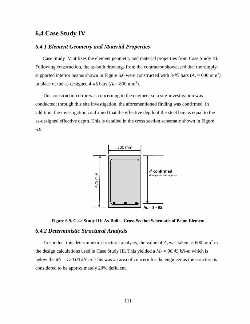
111

6.4 Case Study IV


Case Study IV utilizes the element geometry and material properties from Case Study III.

Following construction, the as-built drawings from the contractor showcased that the simply-

supported interior beams shown in Figure 6.6 were constructed with 3-#5 bars (As = 600 mm2)

in place of the as-designed 4-#5 bars (As = 800 mm2).

This construction error was concerning to the engineer so a site-investigation was

conducted; through this site investigation, the aforementioned finding was confirmed. In

addition, the investigation confirmed that the effective depth of the steel bars is equal to the

as-designed effective depth. This is detailed in the cross section schematic shown in Figure

6.9.

Figure 6.9. Case Study III: As-Built - Cross Section Schematic of Beam Element


To conduct this deterministic structural analysis, the value of As was taken as 600 mm2 in

the design calculations used in Case Study III. This yielded a Mr = 96.45 kN-m which is

below the Mf = 120.00 kN-m. This was an area of concern for the engineer as the structure is

considered to be approximately 20% deficient.

112


Probabilistically, the original as-designed element was reassessed using the new

information from the contractor regarding the missing steel bar resulting in an As = 600 mm2.

Additionally, since the value of effective depth of the steel reinforcement, d, was confirmed

during the site investigation, the statistical parameters (bias and COV) used to calculate the

resistance distribution are the bias and COV values in Table 4.5 which consider the multi-

parameter resistance model where d was defined deterministically at its average value. The

probabilistic structural analysis for the as-built scenario for Case Study IV is presented in

Table 6.8; the as-built β of this element is less than the target β (the as-built Pf is greater than

the target Pf) which would represent deficiency with respect to the Code.

Table 6.8. Case Study IV: Resistance and Load Distributions; β and Pf

Design Bias COV Mean Std. Dev.

Resistance, R * 96.45 kN-m 1.145 0.068 122.71 kN-m 8.34

Dead Load, D 5.14 kN/m 1.05 0.10 5.40 kN/m 0.54

Live Load, L 5.52 kN/m 1.0 0.18 5.52 kN/m 0.99

Load Effect, S - - - 87.34 kN-m 9.05

β * 2.88 Pf * 6.35 × 10-3

βtarget 3.5 Pf 2.3 × 10-3

* Bold values are values that have been updated from Case Study III - Table 6.6


The as-built point, considering the new As and deterministically defining d, is plotted on

Figure 6.10. The as-built Pf point has a higher probability of failure compared to the baseline

Pf limit at a D/(D+L) value of 0.48. This point represents data similar to postulated

deterioration levels of 16.5%. It was deemed appropriate to conduct structural load testing to

determine if the structure can meet the target Pf limit.

However, as can be seen in Figure 6.10, the post-load testing Pf was still greater than the

Pf threshold (i.e. the reliability of the element after load testing was less than the target

reliability threshold). To ensure that the post-load testing reliability is equal to or greater than

the target reliability, an adjustable TLM live load factor was selected from Table 5.2. At a

113

deterioration level approximately equal to 15%, a 5% increase in the TLM live load factor for

ACI 437 Case I and ACI 318 was deemed sufficient to increase the post-load testing

reliability to target reliability levels.

Following the TLM live load factor increase, the resulting Pf level following a successful

load test will be approximately 4.0 × 10-6; this is the Pf at D/(D+L) = 0.48 on the design threshold.

Table 6.9 showcases the TLM calculation for both load tests given a 5% increase in the

TLM live load factor. In practice, it is required to apply this loading using equivalent point

loads based on the given configuration and loading mechanism.

Figure 6.10. Case Study III: As-Built - Probability of Failure Design and Load Testing Limits

Table 6.9. Case Study III: As-Built – Test Load Magnitudes with Live Load Factor Adjustment

Code Provision Test Load Magnitude

ACI 437 Case I TLM = 1.0 DW +1.1 DS +1.68 L+0.5 (LR or S or R)

TLM = 1.0 (3.525) + 1.1 (1.61) + 1.68 (5.52)

TLM437 = 14.57 kN/m

ACI 318 Ch. 27 TLM = 1.15 D +1.575 L+0.4 (LR or S or R)

TLM = 1.15 (5.135) + 1.575 (5.52)

TLM318 = 14.60 kN/m

114

6.5 Conclusions

Figure 6.11 represents the sample outcomes of a successful load test with respect to three

elements with different reliabilities prior to load testing.

Similar to Case Study IV, Sample Point 1 represents an under-designed element as its Pf is

higher than the target Pf level. If the element is successfully load tested, its reliability will

enhance to the Pf level of the test used to complete the load test (as per arrow 1). This

element has a low chance of passing a load test given that its initial estimate of reliability

is less than the design; however, in the likelihood of a successful load test, the improved

post-load testing reliability is significant compared to other scenarios.

Similar to Case Study II and Case Study III, Sample Point 2 represents an adequately

designed element as its Pf is lower than the target Pf level. If the element is successfully

load tested, its reliability will increase to the Pf level of the load test used (as per arrow 2).

Similar to Case Study I, Sample Point 3 represents a significantly over-designed element

such that its Pf is lower than both the target Pf level and the load testing Pf levels. An

element with a reliability beyond the load testing Pf levels is probabilistically much more

likely to pass the load test given the high resistance caused by over-designing the element.

This element lies in a region where load testing has a higher likelihood of success; in the

likelihood of a successful load test, the improved post-load testing reliability is negligible.

Figure 6.11. Expected Outcomes of Load Testing Case Studies and Feasible Testing Regions

115

Chapter 7 Conclusions and Recommendations

7.1 Conclusions

This section summarizes the findings developed throughout this thesis.

7.1.1 Literature Review

The following observations summarize the different facets of load testing that were taken

into consideration during the development of this thesis. The thesis investigated load testing

code provisions, application of load testing, reliability-based design, reliability-based

calibration of design codes, reliability-based load testing concepts, and current load testing

practices in bridge evaluation.

Two load testing code provisions exist under the authority of ACI: ACI 437 and ACI 318

Chapter 27. ACI 437 provides recommendations on structural load testing for both a

monotonic load test and a cyclic load. ACI 318 Ch. 27 provides guidelines on structural

load testing using a monotonic load test. The primary differences between the two code

provisions are the loading protocols (cyclic versus monotonic), the acceptance criteria,

and the dead and live factors used for the test load magnitudes load combinations.

Application studies of load testing provided insight into the similarities and differences of

cyclic load testing versus monotonic load testing. However, the scope of these studies was

usually limited to specific structures (or test experiments) and there was no consideration

given to the differing test load magnitude levels between the two tests; generally, the

application studies of load testing focused on the loading protocols and assessment of

acceptance criteria.

Recent load testing application literature by De Luca et al. (2013) emphasized the need to

transform load testing from a binary, pass-or-fail-outcome testing method into an

informative, diagnostic testing method. It was concluded that a better understanding of the

probability of failure and remaining strength of an element following a load test would

provide valuable insight to practitioners tackling load testing projects.

The concept of reliability-based load testing was developed based on existing literature

which uses conditional probability theory to model proof load testing on structural

116

elements (Hall, 1988). Probabilistically, the concept of conditional probability theory was

determined to be an acceptable method to evaluate the probability of failure of an element

at a given proof load level.

7.1.2 Reliability Assessment of Test Load Magnitudes

Although load testing application and reliability-based load testing literature existed,

there was no existing literature investigating the outcomes of load testing caused by differing

test load magnitudes.

The target reliability levels used throughout this thesis were based on the target reliability

levels calibrated for ACI 318 by Nowak et al. (2012). The test load magnitudes assessed

within this thesis are the TLMs prescribed by ACI 437 and ACI 318 Ch. 27. A MATLAB

model that applied conditional probability theory to the load and resistance distributions

assumed in the calibration of the ACI 318 code at TLM levels prescribed in ACI 437 and ACI

318 Ch. 27 was created. The primary model provided graphical output of the target reliability

and post-load testing reliability. It was determined that:

At as-designed (target) reliability levels, the probability of failure, Pf, of a cast-in-place,

RC beam decreased by approximately an order of magnitude while the Pf of a cast-in-

place, RC slab decreased by approximately 2 orders of magnitude following a load test.

By load testing at the as-designed (target) reliability levels, the reduction in Pf could be

attributed to confirming that the tested element is not one that contains any gross errors or

flaws.

When a deterioration level greater than 10% was postulated, it was determined that the

post-load testing reliability was less than the target reliability for cast-in-place, RC beams;

this implies that a structure may be performing at lower reliability (or higher risk) levels

than assumed in the calibration of the building code even in cases where it may have

successfully passed a load tested.

117

7.1.3 Effects of Site Investigation Findings on Structural Resistance and

Reliability

Chapter 4 focused primarily on conducting an analysis of the flexural resistance model for

cast-in-place, RC beams and cast-in-place, RC slabs. Two methods were considered when

conducting this analysis:

1. Deterministic Parameter Investigation: All components were considered variable based on

their statistical parameters while the component of interest was defined deterministically;

then, the statistical parameters of the resulting resistance model were compared to the

baseline resistance model.

2. Scatter Plot Linear Regression Analysis: The component of interest was kept variable

based on its statistical parameters while all other components were defined

deterministically to their average value. Then, a scatter plot and linear regression analysis

was performed on each parameter of interest versus the resulting resistance.

The main conclusions developed throughout Chapter 4 are summarized as follows:

It was determined that the resistance sensitivity, from the most significant parameter to the

least significant parameter was:


2. Yield strength for reinforcing steel, fy

3. Compressive strength of concrete, f'c (and beam width, b, for cast-in-place, RC

beam)

Through the deterministic parameter investigation, representative resistance statistical

parameters (bias and COV) were developed for cast-in-place, RC beams and slabs

assuming that a material or fabrication property (f’c, fy, d, b) was deterministically defined

through a site investigation. These statistical parameters more accurately represented the

resistance of an element by incorporating site investigation findings.

The refined resistance was then used to develop refined reliability models; by

deterministically defining a material or fabrication property through a site investigation, a

refined estimate of the resistance (and therefore reliability) of an element could be

computed.

118

7.1.4 Test Load Magnitude – Adjustable Live Load Factor

In structures, it was concluded that two scenarios may be considered for the adjustment of

the TLM live load factor:

1. Cast-in-place RC beam experiencing severe deterioration: it was determined that the post-

load testing reliability of cast-in-place, RC beams experiencing severe deterioration levels

(15% or greater) may be less than target reliability levels; this is considering that the

TLMs of ACI 437 CI and ACI 318 Ch. 27 are used for load testing and the target

reliability is as calibrated for use in ACI 318. In such a scenario, even if a load test is

considered successful, the post-load testing reliability may be quantitatively less than the

target reliability.

For beams experiencing severe deterioration (~25% deterioration), it was determined

that a 15% increase in the TLM live load of ACI 437 (αL, ACI 437 = 1.84) and 10%

increase in the TLM live load of ACI 318 Ch. 27 (αL, ACI 318 = 1.65) would permit the

post-load testing reliability to be greater than the target reliability.

2. Cast-in-place RC beam or RC slab following in-depth, favorable site investigation: it was

determined that following a site investigation with favorable outcomes (material or

fabrication properties equal to or greater than their mean value) the as-built resistance of a

cast-in-place, RC beam or RC slab is sufficiently improved. In such a case, it may be

recommended that a practitioner decreases the TLM such that the post-load testing

reliability is in closer proximity to (but always greater than) the target reliability. The

decrease in the TLM live load factor may be chosen to decrease the risk of damaging the

structure while still providing an acceptable confirmation of post-load testing reliability.

For cast-in-place, RC beams, following a favorable site investigation, the TLM live

load factor can be decreased by at least 5% for ACI 437 (αL, ACI 437 = 1.52) and ACI

318 Ch. 27 (αL, ACI 318 = 1.425). Following a favorable site investigation outcome of

effective depth, the TLM live load factor can be decreased by at least 15% for ACI

437 (αL, ACI 437 = 1.36) and ACI 318 Ch. 27 (αL, ACI 318 = 1.28).

For cast-in-place, RC slabs, following a favorable site investigation outcome of

effective depth, the TLM live load factor can be decreased by 15% for both ACI 437

119

and ACI 318 Ch. 27. However, no reduction in TLM live load factor is permitted if

site investigation outcomes of only f’c or only fy were found to be favorable.

7.1.5 Reliability-based Load Testing Case Studies

The first two case studies presented were adapted from load testing application literature;

the third and fourth case studies represented a hypothetical structural assembly. The case

studies were used to showcase how a reliability-based analysis of a structure allows for

improved insight into the probability of failure of an element pre- and post-load testing. It was

demonstrated that reliability-based load testing studies can be used in conjunction with load

testing application to provide supplementary information relating to the reliability of the

investigated element pre- and post-load testing.

7.2 Recommendations

The insights provided in this thesis were based on an analytical, reliability-based

assessment of the American Concrete Institute structural load testing provisions reported in

ACI 437.2-13 and Chapter 27 of ACI 318-14. To supplement the findings presented in this

research and to further develop the practice of load testing from a binary pass-or-fail test into

an informative, diagnostic test, the following recommendations are made:

Reliability-based assessment of load testing projects is encouraged so that engineers,

practitioners, and building officials can gather additional, valuable information about a

structural element or system prior to, during, and following a load test.

Stakeholders involved in the development of load testing codes should give further

consideration to the viability of introducing an adjustable TLM live load factor. This is

especially important for the assessment of cast-in-place, RC beams that have experienced

extensive deterioration.

Consideration should be given to amalgamating the two load testing code provisions

under the authority of ACI as they both fulfill the same purpose.

Further load testing experiments and application case studies that take into consideration

both a varying test load magnitude and the two loading protocols (cyclic and monotonic)

should be developed. The effectiveness of reliability-based load testing could be examined

through feedback received from researchers and practitioners.

120

References

AASHTO. (2014). 2014 Interim Revisions to the Manual for Bridge Evaluation (pp. 8-1 –

816). Washington, DC: American Association of State Highway and Transportation

Officials.

ACI 318-14. (2014). Building Code Requirements for Structural Concrete (ACI 318-14).

Farmington Hills, MI: American Concrete Institute.

ACI 437.1R-07. (2007). Load Tests of Concrete Structures: Methods, Magnitude, Protocols,

and Acceptance Criteria. Farmington Hills, MI: American Concrete Institute.

ACI 437.2-13. (2014). Code Requirements for Load Testing of Existing Structures (ACI

437.2-13) and Commentary. Farmington Hills, MI: American Concrete Institute.

ASCE 7-10. (2013). Minimum Design Loads for Buildings and Other Structures (ASCE/SEI

7-05). Reston, VA: American Society of Civil Engineers.

CAN/CSA-S6-06. (2006). Evaluation. In CAN/CSA-S6-06 Canadian Highway Bridge Design

Code (pp. 675). Mississauga, Ontario, Canada: Canadian Standards Association.

CAN/CSA-S6-06. (2006). Evaluation. In Commentary on CAN/CSA-S6-06 Canadian

Highway Bridge Design Code (p. 562). Mississauga, Ontario, Canada: Canadian

Standards Association.

Casadei, P., Parretti, R., Nanni, A., & Heinze, T. (2005). In Situ Load Testing of Parking

Garage Reinforced Concrete Slabs: Comparison between 24 h and Cyclic Load Testing.

ASCE Practice Periodical on Structural Design and Construction, 40-48.

Casas, J. R., & Gomez, J. D. (2013). Load Rating of Highway Bridges by Proof-loading.

KSCE Journal of Civil Engineering, 556-567.

Cremona, C. (2011). Structural Performance: Probability-based Assessment. Hoboken, NJ:

Wiley.

CSA A.23.3-14 (2014). CSA A23.3-14 Design of Concrete Structures. Mississauga, Ontario,

Canada: Canadian Standards Association.

De Luca, A., Zadeh, H. J., & Nanni, A. (2013). Assessment of Performance of Reinforced

Concrete Strips by In-Place Load Testing. ACI Structural Journal, 813-822.

Ellingwood, B., Galambos, T. V., McGregor, J. G., & Cornell, C. A. (1980). Development of

a Probability Based Load Criterion for American National Standard A58. Cambridge,

MA: U.S. Department of Commerce.

121

Faber, M. H., Val, D. V., & Stewart, M. G. (2000). Proof load testing for bridge assessment

and upgrading. Engineering Structures, 1677-1689.

Galati, N., Nanni, A., Tumialan, J. G., & Ziehl, P. H. (2008). In-Situ Evaluation of Two

Concrete Slab Systems I: Load Determination and Loading Procedure. Journal of

Performance of Constructed Facilities, 207-216.

Hall, W. B. (1988). Reliability of Service-Proven Structures. Journal of Structural

Engineering, 608-624.

Hammad, A., Yan, J., & Mostofi, B. (2007). Recent Development of Bridge Management

Systems in Canada. 2007 Annual Conference of the Transportation Association of

Canada, 1-20.

Liu, Z., & Ziehl, P. H. (2009). Evaluation of Reinforced Concrete Beam Specimens with

Acoustic Emission and Cyclic Load Test Methods. ACI Structural Journal, 288-299.

Nowak, A. S. (1995). Calibration of LRFD Bridge Code. Journal of Structural Engineering,

1245-1251.

Nowak, A. S., & Szerszen, M. M. (2003). Calibration of Design Code for Buildings (ACI

318): Part 1 - Statistical Models for Resistance. ACI Strcutral Journal, 377-382.

Nowak, A. S., Rakoczy, A. M., & Szeliga, E. K. (2012). ACI SP-284-6: Revised Statistical

Resistance Models for R/C Structural Components. ACI Special Publication, 6-1 – 6-16.

Sterman, J. D. (2000). Business Dynamics: Systems Thinking and Modeling for a Complex

World. New York, NY: McGraw-Hill.

Stewart, M. G. (1997). Time-Dependent Reliability of Existing RC Structures. Journal of

Structural Engineering, 896-902.

Szerszen, M. M., & Nowak, A. S. (2003). Calibration of Design Code for Buildings (ACI

318): Part 2 - Reliability Analysis and Resistance Factors. ACI Structural Journal, 383-

391.

Wang, N., Ellingwood, B., & Zureick, A. (2013). Reliability-based framework for improving

highway bridge capacity rating. Safety, Reliability, Risk and Life-Cycle Performance of

Structures and Infrastructures, 3567-3574.

Ziehl, P. H., Galati, N., Nanni, A., & Tumialan, J. G. (2008). In-Situ Evaluation of Two

Concrete Slab Systems II: Evaluation Criteria and Outcomes. Journal of Performance of

Constructed Facilities, 217-227.

122

Appendix A – Reliability-based Assessment of

Bridges Using Structural Load Tests Literature

Review

123

Adapted from a project completed for University of Waterloo CIVE 704: Bridge Design.

Reliability-based Assessment of Bridges Using Structural Load Tests

Amer M. Abu-Khajil, EIT

Abstract

The application of bridge load testing to evaluate structural integrity has existed for many years; nevertheless, reliability-based analyses of load testing can provide further information about assessing and upgrading bridges’ load ratings. As the population of aging bridges increases, reliability concerns continue to rise due to deterioration concerns and increasing traffic loads and densities. Given the aging population of bridges that require feasible assessments, reliability-based load testing methods to assess reliability or upgrade load rating are gaining in popularity. This paper will consider both code provisions relating to load testing and landmark journal articles investigating reliability-based proof load testing.

1. Introduction

Based on Recent Development of Bridge Management Systems in Canada, more than 40% of bridges currently used in Canada are more than 50 years old (Hammad, Yan, & Mostofi, 2007). Figure A.1 presents the sample distribution of time of construction of transportation structures in Quebec; this data includes 4300 provincial bridges, 4400 municipal bridges, and the remaining units are retaining walls and other transportation structures. As can be seen, approximately 60% of transportation structures in Quebec are more than 50 years old.

Figure A.1. Distribution of Time of Construction of Transportation Structures in Quebec

(Hammad, Yan, & Mostofi, 2007)

Over this time period, even with regular inspections, structural deterioration is unavoidable due to material degradation, corrosion, and fatigue. It is typical to assume that many aging bridges will require replacement or structural rehabilitation; however, a significant portion of existing bridges could

124

continue being used if a reliable method of assessing and confirming their load carrying capacity is achieved.

An analytical bridge assessment, considering effects such as deterioration and real truck load data, could provide a baseline of the predicted capacity of a bridge. It is important to consider that the in-situ strength of an existing bridge is typically higher than analytical strength.

Proof load testing is the process of applying a test load on a structural system or element to confirm its satisfactory performance; a successful proof load test states that resistance of the tested structural system or element is greater than the level of the proof load test.

Using a proof load test, the structural capacity can be confirmed and refined to reduce uncertainty and analysis conservatism. Thus, the service life of a bridge could be extended providing a financial incentive over avoidable rehabilitation. However, there are some implications of an unsuccessful load test. There is an inherent risk associated with conducting the test: the test may damage the structure. Additionally, extensive proof load testing could cost up to 6% of a bridge replacement cost (Faber, Val, & Stewart, 2000).

2. Reliability Theory

To best understand the reliability-based method of applying proof load testing to a bridge element or system, the basics of structural reliability theory must be reviewed.

2.1 Design Reliability

Design reliability of structural elements considers the resistance and load effects distributions – R and S distribution, respectively. The probability of failure, Pf, is the probability where the load effect, S, is greater than the resistance, R. Reliability is defined as the likelihood of successful performance and is equal to (1 – Pf). For normally distributed distributions, the reliability index, β, can be defined as:

𝑃𝑓 = 𝑃(𝑅 − 𝑆 < 0) ≈ Φ(𝛽)

, where Φ is the cumulative probability function of a standard normal variable (Cremona, 2011).

Where both the resistance and load effects distributions are normal probability density functions, the reliability index, β, can be defined as:

𝛽 = 𝜇𝑅− 𝜇𝑆

√𝜎𝑅2+ 𝜎𝑆

2 Equation (1)

, where μR = mean of resistance; σR = standard deviation of resistance; μS = mean of load effects; σS =

standard deviation of load effects (Cremona, 2011).

2.2 Load Test Reliability

Conditional probability is defined as the probability of an occurrence of an event given that another event has already occurred. In load testing, the resistance distribution of a bridge element or system is updated given that the structure has survived the applied test load.

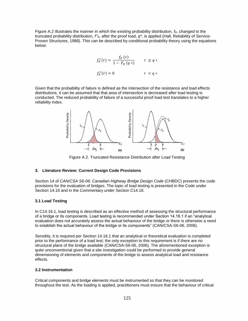
125

Figure A.2 illustrates the manner in which the existing probability distribution, fR, changed to the truncated probability distribution, f’’R, after the proof load, q*, is applied (Hall, Reliability of Service-Proven Structures, 1988). This can be described by conditional probability theory using the equations below:

𝑓𝑅′′(𝑟) =

𝑓𝑅 (𝑟)

1 − 𝐹𝑅 (𝑞 ∗) 𝑟 ≥ 𝑞 ∗

𝑓𝑅′′(𝑟) = 0 𝑟 < 𝑞 ∗

Given that the probability of failure is defined as the intersection of the resistance and load effects distributions, it can be assumed that that area of intersection is decreased after load testing is conducted. The reduced probability of failure of a successful proof load test translates to a higher reliability index.

Figure A.2. Truncated Resistance Distribution after Load Testing

3. Literature Review: Current Design Code Provisions

Section 14 of CAN/CSA S6-06: Canadian Highway Bridge Design Code (CHBDC) presents the code provisions for the evaluation of bridges. The topic of load testing is presented in the Code under Section 14.16 and in the Commentary under Section C14.16.

3.1 Load Testing

In C14.16.1, load testing is described as an effective method of assessing the structural performance of a bridge or its components. Load testing is recommended under Section 14.16.1 if an “analytical evaluation does not accurately assess the actual behaviour of the bridge or there is otherwise a need to establish the actual behaviour of the bridge or its components” (CAN/CSA-S6-06, 2006).

Sensibly, it is required per Section 14.16.1 that an analytical or theoretical evaluation is completed prior to the performance of a load test; the only exception to this requirement is if there are no structural plans of the bridge available (CAN/CSA-S6-06, 2006). The aforementioned exception is quite unconventional given that a site investigation could be performed to provide general dimensioning of elements and components of the bridge to assess analytical load and resistance effects.

3.2 Instrumentation

Critical components and bridge elements must be instrumented so that they can be monitored throughout the test. As the loading is applied, practitioners must ensure that the behaviour of critical

126

components and elements of the bridge are acting as expected in the analysis. If there are any deviations from an expected response, testing must be stopped to ensure components and elements do not fail or are overstressed (CAN/CSA-S6-06, 2006).

3.3 Test Load Procedure

The CHBDC prescribes either a static or dynamic loading procedure for the load test.

Static loading is applied using full-sized test trucks or by jacking loads into the bridge; these loads are to be placed at predetermined locations on the bridge. Loading patterns are applied such that critical components and elements experience the maximum load effects. Static loading is to be applied until one of the following conditions occurs:

(a) “the measured strain or displacement deflection increments start deviating from linearity.” Once the structural component or elements experiences non-linear behaviour, it is expected that the structural behaviour has changed or that the induced deflections may not be recoverable;

(b) the loading equipment is loaded to its capacity; or,

(c) A maximum predetermined loading is achieved (Commentary on CAN/CSA-S6-06, 2006).

Dynamic loading is applied using testing vehicles or normal traffic. Dynamic loading is typically used to better understand or identify the dynamic amplifications of the static effects. The behaviour of the bridge is monitored under:

(a) test vehicles with known axle loads only;

(b) normal traffic conditions; or,

(c) other approved methods (Commentary on CAN/CSA-S6-06, 2006).

3.4 Live Load Capacity

For static loading condition (a), where the observed behaviour indicates non-linear deformations, the maximum applied test load may be assumed to be representative of the ultimate capacity.

For static loading conditions (b) and (c), test results can be extrapolated, as necessary, to determine the live-load-carrying capacity. Extrapolation is to be conducted by establishing an acceptable level of maximum strain and then predicting, using approved methods, which load level would achieve that strain.

3.5 Evaluation Using Observed Behaviour

Within CHBDC C14.16.4.1, a discussion of anticipated bridge behaviour during testing is presented. It is recommended that practitioners rationalize the behaviour before considering any change in strength concluded from the testing. Some of the behaviours to consider when analyzing load testing results include composite action in non-composite decks, load sharing in trusses, seized bearings, and out-of-place bending of vertical members.

3.6 Current Design Code Provisions: Concluding Remarks

As can be observed, the CHBDC provides a general overview of load testing within Chapter 14: Evaluations. The CHBDC does not provide any specific loading limits or acceptance criteria for the load test. The loading limits are only confined by the structure’s capability to resist those loads within its linear behaviour. The acceptance criteria of load testing are defined by the structural behaviour’s shift towards non-linearity. These general parameters place the control of the load testing assessment in the hands of the practitioner. Therefore, load testing procedures, instrumentation, loading, and

127

evaluation should be conducted by a qualified practitioner with previous experience to minimize the potential of permanently damaging the structure after load testing.

Notably, the load testing provisions with the CHBDC do not discuss the use of load testing to assess or update the load rating of bridges. No discussion of reliability-based approaches to attain target proof load levels or target reliability indices is provided in the CHBDC. The CHBDC only presents load testing as a means of confirming structural performance.

4. Literature Review: Journal Papers

The following landmark papers provide theoretical and practical insight into the process of load testing of bridges beyond the scope of load testing provided in CHBDC Section 14.16.

1. Reliability-based Framework for Improving Highway Bridge Capacity Rating.

N. Wang; B. R. Ellingwood; A. Zureick. 2013.

2. Load Rating of Highway Bridges by Proof-Loading.

J. R. Casas; J. D. Gomez. 2013.

3. Proof Load Testing for Bridge Assessment and Upgrading.

M. H. Faber; D. V. Val; M. G. Stewart. 2000.

4.1 Reliability Considerations Prior to Load Testing

In each of the reviewed documents, considerable discussion is included relating to transforming the deterministic analyses to reliability, or probabilistic, analyses. Deterministic analyses tend to consider the most conservative assumptions in conducting an analysis to accommodate for uncertainties. Conversely, a reliability-based analysis collects all available information about resistance and loading that may influence the outcome. This reliability-based approach allows for better-informed decision making.

To assess the resistance and load distributions prior to load testing, these uncertainties must be considered:

(a) representing real structures by idealized models (model error);

(b) material property variation;

(c) variability in workmanship and element dimensions;

(d) variability of in-service loading; and,

(e) assessment of deterioration processes currently affecting the structure (Faber, Val, & Stewart, 2000).

Each of these uncertainties can be probabilistically defined through different methods. (a) can be estimated by an experienced practitioner as the expected margin of error between the probabilistic analysis and the real structure. (b) and (c) can be defined by data from existing literature on the variability of material properties and element dimensions. (d) can be estimated by conducting load monitoring on the structure over a predetermined period of time. (e) can be estimated by conducting a thorough site inspection by a qualified investigator to assess fatigue, corrosion, and other deterioration mechanisms affecting the structure.

For example, to accommodate for (d) variability of in-service loading, a detailed method of defining lifetime load effects of traffic on highway bridges is described in Load Rating of Highway Bridges by Proof-Loading by Casas and Gomez. Characteristic, 50-year mean, and 50-year COV of lifetime load effects are defined for 5 European counties with respect to lane density and approximate bridge span.

128

Another consideration related to load testing involves test risk: the likelihood that a load test will incur permanent damage to the structure. A structure could experience non-linear behaviour and non-recoverable deformation if continuous monitoring is not conducted. However, test risk is extremely small if proper planning, execution, and monitoring is conducted. Of more than 250 bridge tests conducted in Ontario, not a single bridge suffered any test-related damage (Casas & Gomez, 2013). The failure mechanism of the structure, whether ductile or sudden, should be carefully understood prior to load testing.

4.2 Paper #1: Reliability-based Framework for Improving Highway Bridge Capacity Rating (2013)

Wang et al. argue that analytical methods specified in AASHTO Manual of Bridge Evaluation provide unnecessarily conservative load rating results. Since bridge maintenance decisions are influenced by the load rating of a bridge, this undue conservatism could cause economic repercussions when it comes to the rehabilitation or replacement of sufficiently serviceable structures. However, load ratings concluded from proof load testing, which are more representative of realistic, in-situ behaviour of the bridge, are too costly and possess a test risk. This paper focuses on providing a framework that considers the use of both in-situ data and “virtual” proof load testing using finite element analysis to provide a more cost-effective and realistic representation of the structure.

4.2.1 Paper #1: Methodology

The 52-year old, straight, reinforced concrete, T-beam bridge shown in Figure A.3 selected as the test bed for this study as it was scheduled for demolition. To determine in-situ material strengths, seven cores were taken from the concrete slab at seven different locations. Additionally, fourteen cores were taken from various girders along the bridge. It was determined that the mean strength of f’c is 1.93 times the specified compression strength; this time-dependent increase is typical for good-quality concrete. The increased in-situ f’c value provides significant improvements to the shear capacity, over 30% increase, and modest improvements to the moment resistance of the bridge (Wang, Ellingwood, & Zureick, 2013).

To create calibrated FE models, three-dimensional, nonlinear representations of this structures and three other similar bridges was developed. The FE models considered failure modes, strength-reduction caused by cracking, realistic boundary conditions, and rebar-to-concrete compatibility, amongst other factors. Realistic data from the in-situ investigation was used within the input of material properties.

4.2.2 Paper #1: Results

By experimentally conducting the load test, the maximum bending moment and deflections were well within the limits stipulated in AASHTO LRFD; thus, it is concluded that a significant margin of safety was incorporated into the code provisions.

Once both FE and experimental data was recovered, a comparison was conducted between the “virtual” FE testing and the experimental measurements. The comparison investigated each of the four girders at different loading levels. Figure A.4 showcases a sample of the results for the girders loaded by the full test load: four GOT test trucks. The maximum noted discrepancies were within a 20% limit; however, in most cases, the model was significantly more accurate.

129

Figure A.3. Straight, RC T-Beam Bridge

Figure A.4. Girder Displacement –

Measured Data vs. FE Analysis

(Wang, Ellingwood, & Zureick, 2013)

4.2.3 Paper #1: Conclusions

By calibrating a FE model using similar bridges and in-situ material properties, a “virtual” load test may provide outcomes that are comparable to an experimental proof load test. Although this is obviously tedious and impractical, if a database of tested structures and their response was created, “virtually” proof load testing could provide practical results that are more accurate than deterministic analytical principles. Although these analyses will differ from one bridge to another, the collection of in-situ data combined with intelligent modeling methods could yield methods of evaluation that are more accurate and cost-effective than conservative, deterministic analyses or costly, relatively-risky load testing.

4.3 Paper #2: Load Rating of Highway Bridges by Proof-Loading (2013)

The goal of Casas and Gomez’s paper was to create a systematic method to develop target proof load factors based on target reliability levels. The primary purpose is to develop a framework that facilitates proof load testing of bridges for various European Union countries based significantly varied traffic loadings. In this work, the method to calculate the target proof load factor is based on a reliability-based approach proposed in ARCHES and AASHTO. However, this reliability-based approach is not explicitly outline in the CHBDC.

4.3.1 Paper #2: Methodology

Five countries were selected to represent the variable truck load traffic present in the European Union. For each of the countries, traffic effects are considered for different lane factors and spans. The characteristic value, 50-year mean, and 50-year COV of the midspan moment are calculated using Monte Carlo Simulations and simple statistical projection techniques. The investigation of load effects is extensive given that the purpose of the paper is to review the differences of these load effects between the different locations within the European Union for enhanced selection of proof load testing load factors (Casas & Gomez, 2013).

Using a database of values on different bridge types and spans, then using calculated permanent and traffic loads, the nominal resistance, Rn, is assessed. The resistance, R, is calculated using bias and COVs from literature.

Then by combining these large datasets of loads from each of the countries and the R/Rn ratio, target proof load factors can be calculated for each country for different spans based on predetermined target reliability values.

130

4.3.2 Paper #2: Results

To facilitate the process of calculating target proof load factors that provide target reliability levels after testing, large data sets of traffic loads are used to represent different countries. This makes it easier for practitioners to select proof load factors depending on the safety levels the structure aims to achieve. A sample of results is shown in Table A.1. As can be seen, practitioners can consult these tables to determine the necessary target proof load factor to run the load test.

Table A.1. Target Proof Load Factors for Czech Republic Traffic and Reliabil ity Values

(Casas & Gomez, 2013)

4.3.3 Paper #2: Conclusions

Although this data effectively summarized target proof load factors for different countries throughout the EU, the authors note that these may be too conservative for some situations – especially for highways on local or secondary roads. The tabulated version of this data is useful; however, given that the purpose of defining the proof load factors is crucial to conducting the test, the tabulated values may provide unnecessary conservatism which may be comparable to conservative results from the analytical assessments. It is important that the assessment of bridges is not overly conservative so that satisfactory bridges are not unnecessarily rehabilitated or replaced.

4.4 Paper #3: Proof Load Testing for Bridge Assessment and Upgrading (2000) Similar to the outcomes presented in Load Rating of Highway Bridges by Proof-Loading by Casas and Gomez, Faber et al. utilize the reliability-based concept of proof load testing to allow practitioners to extract the proof load intensity, or factor, to maintain or increase load ratings. Based on the selected proof load intensity and the age of the bridge at the time of load testing, the test reliability could be attained. The analysis also considers two postulated deterioration scenarios. 4.4.1 Paper #3: Methodology The resistance and load effects of the bridge are modelled based on an analysis of variability from existing literature and codes. To accommodate for time-dependent structural reliability, considering the reliability of a bridge at the time of load testing, a time variant reliability analysis component was added to the analysis. Additionally, a degradation function from existing literature was adopted to accommodate for low and medium deterioration levels based on the age of the structure. To accommodate and represent various bridge spans and types, three different types of dead to live load ratios, ρ, are represented in the analysis. By adopting the methodology of reliability-based load testing presented in Section 3.2, the test load magnitude of the test is selected based on a percentage of the characteristic live load used in the

131

initial design of the bridge. The assumed target reliability is equal to 3.4 for an intended design life of 100 years. 4.4.2 Paper #3: Results By distinctly applying the reliability-based concepts of load testing, a series of graphs were generated to represent the data. A sample of the final results is illustrated in Figure A.5 below.

For example, once a deterioration level, dead to live load ratio, and age of the bridge are determined, practitioners can select a load rating that they wish to achieve (100%, 105%, 110%, 115%). Using Figure 5.a, the proof load intensity to be used is selected. Then, using Figure 5.b and the selected proof load intensity, the test reliability can be determined (Faber, Val, & Stewart, 2000). The test reliability describes the probability of the bridge successfully surviving the load test.

Figure A.5. 'Low deterioration', Vr = 0.15, ρ = 2, and different bridges ages:

(a) required proof load intensit ies; (b) test reliabil ity (Faber, Val, & Stewart, 2000).

4.4.3 Paper #3: Conclusions Faber et al. present these complex outcomes graphically which allows for a more flexible selection of load intensities and identification of test reliability. By considering time-dependent, reliability-based proof load testing, Faber et al. were capable of providing probabilistic inferences about bridge assessment and upgrading. The practical findings developed in this work provide practitioners with a general foundation to adequately select proof load intensities based on desired levels of reliability necessary for assessment.

5. Conclusions

As more of the population of in-service bridges experiences deterioration and distress, stakeholders are seeking definitive methods of evaluation that would accurately assess structural integrity and reliability. Load testing, when performed correctly, is emerging as a means of providing an accurate, in-situ health assessment of the bridge. Understanding the reliability of a bridge using load testing allows for better decision making with respect to whether rehabilitation or replacement is needed over conventional analysis methods.

132

Appendix B – Base MATLAB Code

133

function ACILoadTest (ElementAndFailureMode, LoadCase, DeterOccPercent, DETAILS)

%% Selection of the element type;

% Statistical parameters of resistance (bias and COV)

% Rprop = [BIAS COV PHI]

if ElementAndFailureMode == 'B' Rprop = [1.021 0.061 0.90]; element= 'Beam, flexure [Nowak, 2012]'; elseif ElementAndFailureMode == 'S' Rprop = [1.055 0.145 0.90]; element= 'Slab, flexure [Nowak, 2012]'; else outputA= 'Please review input arguments'; end

%% Selection of governing load case;

if LoadCase == 1 scenario = 'Dead + Live'; elseif LoadCase == 2 scenario = 'Dead + Live + Snow; live load dominates'; else outputB = 'Please review input arguments; Load Case value must equal 1 or 2'; end

%% Setting-up D/(D+L) Loading Values

DLratio = 0.02 : 0.01 : 0.99; % D/(D+L) values from 0.02 to 0.99 @ 0.01 DwDsratio = [0.25 0.5 0.75 1]; % Dead w to Dead s Ratios: 0.25, 0.5, 0.75, 1 Dcomp = 1; % D component for D/(D+L) values Dw = Dcomp * DwDsratio; % Dw = 0.25, 0.5, 0.75, 1 Ds = Dcomp - Dw; % Ds = 0.75, 0.5, 0.25, 0 Lcomp = (Dcomp - DLratio) ./ DLratio; % L components for D/(D+L) increments Scomp = 0.5 .* Dcomp; % S = 0.5L as per Nowak & Szerszen (2003)

%% Setting-up Load Statistical Parameters % [Bias COV] Dprop1 = [1.05 0.10]; % Dead Load (cast-in-place) Lprop1 = [1.00 0.18]; % Live Load Dominating Sprop = [0.20 0.87]; % Snow Load Point-in-Time

% Dead Load Components MeanD = Dcomp * Dprop1(1); % Mean of Dead Load component StdDevD = MeanD * Dprop1(2); % Standard Deviation of Dead Load component

% Live Load Components; where *Live is dominating* MeanL1 = Lcomp .* Lprop1(1); % Mean of Live Load at each D/(D+L) StdDevL1 = MeanL1 .* Lprop1(2); % Std Dev of Live Load at each D/(D+L)

% Nominal Snow Load Parameters; where *Snow is NOT dominating* MeanS1 = Scomp .* Sprop(1); % Mean Snow Load at each D/(D+L) StdDevS1 = MeanS1 .* Sprop(2); % Std Dev of SNow Load at each D/(D+L)

%% Load Probability Density Function: % Calculates the MeanS and StdDevS to generate the Load Distribution % Case 1: D + L % Case 2: D + L + S ; where L dominates

134

if LoadCase == 1 MeanS = (MeanD + MeanL1); StdDevS = sqrt(StdDevD.^2 + StdDevL1.^2); elseif LoadCase == 2 MeanS = (MeanD + MeanL1 + MeanS1); StdDevS = sqrt(StdDevD.^2 + StdDevL1.^2 + StdDevS1.^2); end

%% Design Resistance Probability Density Function [index 1]: % Calculates the MeanR1 and StdDevR1 to generate DESIGN (TARGET) % Resistance Distribution (index 1) and the associated % beta & Pf values. % ~~~ NOTES ~~~ % Rprop(3) is the phi value associated with the element % The Load Factors are defined by ACI 318-11 (Page 119-120)

if LoadCase == 1 Rfact1(1:87) = (1/Rprop(3)) .* (1.2 * Dcomp + 1.6 .* Lcomp(1:87)); Rfact1(88:98) = (1/Rprop(3)) .* 1.4 * Dcomp; elseif LoadCase == 2 Rfact1 = (1/Rprop(3)) .* (1.2 * Dcomp + 1.6 .* Lcomp + 0.5 .* Scomp); end

MeanR1 = Rfact1 .* Rprop(1); StdDevR1 = MeanR1 .* Rprop(2); beta1 = (MeanR1 - MeanS)./(sqrt(StdDevR1.^2 + StdDevS.^2)); Pf1 = normpdf(beta1);

%% Deteriorated Resistance Probability Density Function [index 2]: % Calculates the MeanR2 and StdDevR2 to generate DETERIORATED % Resistance Distribution (index 2) and the associated % beta & Pf values

% ~~~ NOTES ~~~ % The deterioration is a percent change to the mean of the original (design) R

MeanR2 = MeanR1 .* ((100 - DeterOccPercent)/100); StdDevR2 = MeanR2 .* Rprop(2); beta2 = (MeanR2 - MeanS)./(sqrt(StdDevR2.^2 + StdDevS.^2)); Pf2 = normpdf(beta2);

%% ACI 318 24-hour Load Test* [load test index 1]: % Uses Trapezoidal Rule to approximate Pf at each D/(D+L) using % the DETERIORATED resistance properties (i.e. the test load is applied % onto the deteriorated element). The TLM is based on the ACI 318 TLM

if LoadCase == 1 TLM1(1:90) = 1.15 .* Dcomp + 1.5 .* Lcomp(1:90); TLM1(90:98) = 1.3 .* Dcomp; elseif LoadCase == 2 TLM1 = 1.15 .* Dcomp + 1.5 .* Lcomp + 0.4 .* Scomp; end

135

% Numerical Integration algorithm to calculate probability of failure using

% conditional probability

sizeTLM = size(TLM1); FrTLM = normcdf(TLM1, MeanR2, StdDevR2);

for i = 1:sizeTLM(2), X1 = TLM1(i):0.001:(TLM1(i)+100); calc = normcdf(X1, MeanS(i), StdDevS(i)) .* normpdf(X1, MeanR2(i),StdDevR2(i)); trapzint = trapz(X1, calc); PfTLM1(i) = 1 - ((1/(1-normcdf(TLM1(i), MeanR2(i), StdDevR2(i)))) * trapzint); end

%% ACI 437 Cyclic Load Test Case 1 [load testing index 2]: % Uses Trapezoidal Rule to approximate Pf at each D/(D+L) using % the DETERIORATED resistance properties (i.e. the test load is applied % onto the deteriorated element). The TLM is based on ACI 437 Case I.

for j = 1:length(Dw) if LoadCase == 1 TLM2(1:85) = Dw(j) + 1.1 .* Ds(j) + 1.6 .* Lcomp(1:85); TLM2(86:98) = 1.3 * (Dw(j) + Ds(j)); elseif LoadCase == 2 TLM2 = Dw(j) + 1.1 .* Ds(j) + 1.6 .* Lcomp + 0.5 .* Scomp; end


for i = 1:sizeTLM(2), X1 = TLM2(i):0.001:(TLM2(i)+100); calc = normcdf(X1, MeanS(i), StdDevS(i)) .* normpdf(X1, MeanR2(i),StdDevR2(i)); trapzint = trapz(X1, calc); PfTLM2(i, j) = 1 - ((1/(1-normcdf(TLM2(i), MeanR2(i), StdDevR2(i))))*trapzint); end end

%% ACI 437 Cyclic Load Test Case 2 [load testing index 3]: % Uses Trapezoidal Rule to approximate Pf at each D/(D+L) using % the DETERIORATED resistance properties (i.e. the test load is applied % onto the deteriorated element). The TLM is based on ACI 437 Case II.

for j = 1:length(Dw) if LoadCase == 1 TLM3(1:89) = Dw(j) + 1.1 .* Ds(j) + 1.4 .* Lcomp(1:89); TLM3(90:98)= 1.2 * (Dw(j) + Ds(j)); elseif LoadCase == 2 TLM3 = Dw(j) + 1.1 .* Ds(j) + 1.4 .* Lcomp + 0.4 .* Scomp; end

136


for i = 1:sizeTLM(2), X1 = TLM3(i):0.001:(TLM3(i)+100); calc = normcdf(X1, MeanS(i), StdDevS(i)).* normpdf(X1, MeanR2(i), StdDevR2(i)); trapzint = trapz(X1, calc); PfTLM3(i, j) = 1 - ((1/(1-normcdf(TLM3(i), MeanR2(i), StdDevR2(i))))* trapzint); end

end

%% Plot Design, Deteriorated, ACI 318 Pf, ACI 437 CI Pf, and ACI 437 CII Pf. % It is assumed that the dead weight and the superimposed dead load are % each one half of the dead load component.

if DETAILS == 0 figure('Position', [0, 0, 600, 600]);

semilogy(DLratio, Pf1,'k','LineWidth',1.5); % plot Design case Pf hold on

semilogy(DLratio, Pf2,'r','LineWidth',2); % plot Deteriorated case hold on

semilogy(DLratio, PfTLM1,'b:', 'LineWidth',1.5); % plot ACI 318 Test hold on

semilogy(DLratio, PfTLM2(:,2), 'g-.', 'LineWidth',1.5); % plot ACI 437 Case I hold on

semilogy(DLratio, PfTLM3(:,2), '--m', 'LineWidth',1.5); % plot ACI 437 Case II %hold on

Title ({'Probability of Failure: Design and Load Testing Cases', element, ...

[scenario ' at \phi =' num2str(Rprop(3))]}, 'FontSize', 12, 'FontWeight', ...

'bold'); xlabel('D/(D+L)', 'FontSize',12); ylabel('Pf', 'FontSize',12); axis([0 1 0.00000001 1]);

legend({'Overall Design', ...

'Postulated Deterioration ' num2str (DeterOccPercent) '%'], ...

'Post-ACI 318 - Deteriorated Member', ...

'Post-ACI 437 C1 - Deteriorated Member', ... 'Post-ACI 437 C2 - Deteriorated Member'}, 'Location', 'SouthOutside'); end

137

Appendix C – Scatter Plot Linear Regression

Analysis: Effects of Material and Fabrication

Properties on Structural Resistance

138

CIP Beam (ρ = 0.6%) – Linear Regression Sensitivity Analysis Results

By considering a linear regression sensitivity analysis for the effects of f’c on the

resistance of a beam element, variable parameters were set deterministically to their average

values. The As, fy, d, and b were set equal to their average values while f’c remained variable.

Figure C.1 plots the resulting f’c values and their associated resistance; then, a linear trendline

is plotted along the data set resulting in a coefficient of determination (r2) equal to 0.0132.

Next, to conduct a linear regression sensitivity analysis for the effects of fy on the

resistance of a beam element, variable parameters (As, f’c, d, and b) were set deterministically

to their average values while fy remained variable. Figure C.2 plots the scatter plot regression

analysis results for fy ; the resulting r2 is equal to 0.1891.

Finally, to conduct a linear regression sensitivity analysis for the effects of d on the

resistance of a beam element, variable parameters (As, f’c, fy, and b) were set deterministically

to their average values while d remained variable. Figure C.3 plots the scatter plot regression

analysis for d; the resulting r2 is equal to 0.3142.

Figure C.1. Scatter Plots of f’c versus Moment Resistance for a CIP Beam Element (ρ = 0.6%)

139

Figure C.2. Scatter Plots of fy versus Moment Resistance for a CIP Beam Element (ρ = 0.6%)

Figure C.3. Scatter Plots of d versus Moment Resistance for a CIP Beam Element (ρ = 0.6%)

The OAT scatter plot linear regression was performed by sampling each variable

parameter of interest (f’c, fy, and d) against the moment resistance; this was conducted to

determine the relative effects of the investigated parameters on the output (moment

resistance). The coefficient of determination, r2, and the correlation coefficient, r, were used

to model the linear relationship between each random variable and the resulting value of the

moment resistance. Values of r close to +1 or -1 indicate a higher confidence in predicting

resistance using the investigated random variable. Values of r2 close to 1 indicate that the

140

trend line fits the data; r2 values close to 0 indicate there is not a statistically significant

relationship between the input and the output.

As can be clearly seen in Table C.1, the effective depth had the highest effect on the

resistance of a beam element while f’c had the lowest effect on the resistance of a beam

element investigated under flexure. The results from the linear regression sensitivity analysis

match the conclusions identified previously in the deterministic parameter investigation.

Table C.1. CIP, RC Beam Element, Coefficient of Determination (r2) and Correlation Coefficient (r)

MC Simulation

(N = 105 trials)

Random Variable

Coefficient of

Determination

(r2)

Correlation

Coefficient

(r)

f'c 0.0132 0.1149

fy 0.1891 0.4349

Effective Depth, d 0.3142 0.5605

CIP Slab (ρ = 0.3%) – Linear Regression Sensitivity Analysis Results

By considering a linear regression sensitivity analysis for the effects of f’c on the

resistance of a slab segment, variable parameters were set deterministically to their average

values. The As, fy, and d were set equal to their average values while f’c remained variable.

Figure C.4 plots the resulting f’c values and their associated resistance; then, a linear trendline

is plotted along the data set resulting in a r2 equal to 0.0080. This can be compared to r2 =

0.0132 for the sensitivity associated with f’c for a beam element. A value of r2 ≈ 0 indicates a

statistically insignificant relationship between f’c and the resistance. Thus, f’c can be

considered to have an insignificant effect on R.

Next, to conduct a linear regression sensitivity analysis for the effects of fy on the

resistance of a slab segment, variable parameters (As, f’c, and d) were set deterministically to

their average values while fy remained variable. Figure C.5 plots the scatter plot regression

analysis results for fy; the resulting r2 is equal to 0.1879. This value was very similar to r2 =

0.1891 associated with the sensitivity of fy for a beam element. When fy is considered relative

141

to the other resistance parameters, it can be concluded that fy had an equivalent effect on the

resistance of cast-in-place, RC beams and cast-in-place, RC slabs.

By setting As, f’c, and fy deterministically to their average values while d remained

variable, the effects of d on the moment resistance of a slab segment was examined. Figure

C.6 illustrates the scatter plot regression analysis for of d; the resulting r2 is 0.8088. For

comparison, the r2 value for the effective depth of a CIP, RC beam was 0.3142. The effective

depth had the most significant effect on the moment resistance of both cast-in-place RC

beams and cast-in-place RC slabs; however, the effective depth had a significantly higher r2

value in slabs compared to beams. A small change in the effective depth of a slab is

associated with a significant change in its moment resistance.

Figure C.4. Scatter Plots of f’c versus Moment Resistance for a CIP Slab Segment (ρ = 0.3%)

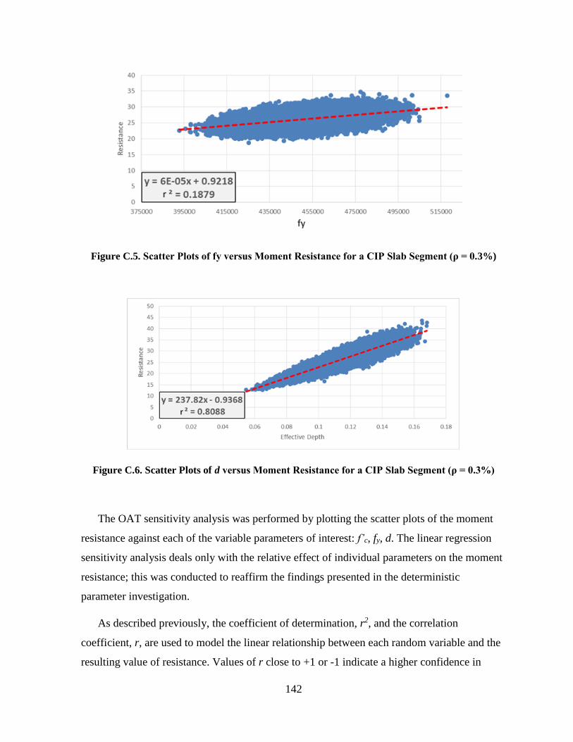
142

Figure C.5. Scatter Plots of fy versus Moment Resistance for a CIP Slab Segment (ρ = 0.3%)

Figure C.6. Scatter Plots of d versus Moment Resistance for a CIP Slab Segment (ρ = 0.3%)

The OAT sensitivity analysis was performed by plotting the scatter plots of the moment

resistance against each of the variable parameters of interest: f’c, fy, d. The linear regression

sensitivity analysis deals only with the relative effect of individual parameters on the moment

resistance; this was conducted to reaffirm the findings presented in the deterministic

parameter investigation.

As described previously, the coefficient of determination, r2, and the correlation

coefficient, r, are used to model the linear relationship between each random variable and the

resulting value of resistance. Values of r close to +1 or -1 indicate a higher confidence in

143

predicting resistance using the investigated random variable. Values of r2 close to 1 indicate

that the trend line fits the data; r2 values close to 0 indicate there is not a statistically

significant relationship between the input and the output.

As can be clearly seen in Table C.2, the effective depth had the highest effect on the

resistance of a slab segment while f’c had the lowest, and practically negligible, effect on the

resistance of a slab segment investigated under flexure.

It is also important to note that the resistance was significantly more sensitive to the

effective depth in slab segments compared to beam elements. Accurately placing and

confirming the placement of rebar in a slab, by determining the effective depth, is crucial

given that a small decrease in the effective depth of a slab may cause significant decrease in

the ability of the slab to resist moments.

The results from the linear regression sensitivity analysis match the conclusions identified

in the deterministic parameter investigation.

Table C.2. CIP, RC Slab Segment Coefficient of Determination (r2) and Correlation Coefficient (r)

MC Simulation

(N = 105 trials)

Random Variable

Coefficient of

Determination

(r2)

Correlation

Coefficient

(r)

f'c 0.0080 0.0894

fy 0.1879 0.4335

Effective Depth, d 0.8088 0.8993

144

Appendix D – Deterministic Parameter

Investigation: Additional Results

145

CIP Beam (ρ = 0.6%) – Multiple Parameter Combinations Deterministic

To further investigate the multi-parameter model sensitivity, combinations of multiple

parameters were set deterministically. Two cases were investigated:

A. f’c and fy are deterministic; and,

B. f’c, fy, and d known.

As can be seen when f’c and fy are deterministic (Case A), the resulting bias = 1.145 and

COV = 0.075 are approximately equivalent to the case where only fy is set to its average value

(λ= 1.147 and a COV = 0.075). Therefore, as concluded previously, deterministically setting

f’c contributes a very small effect to the reliability of a beam section in flexural.

Figure D.1. Beam - Multi-Parameter Resistance Model: Baseline PDF and PDF for f’c and fy =

average

Table D.1. Beam - Multi-Parameter Resistance Model: Bias & COV (f’c and fy = average)

MCS Input [MPA]

(f’c = 30)

(fy = 400)

Resistance

Bias COV

MP Baseline f’c = variable

fy = variable 1.145 0.080

Average f'c = 36.57

fy = 452 1.145 0.075

146

For Case B, where f’c, fy, and d are deterministic, the resulting bias = 1.145 and COV =

0.062. The change in COV for Case B is equal to 0.018 which is similar to the superposition

of the change in COV from fy (0.005) and d (0.012). Table D.2 showcases the resulting bias

and COV for case B.

Figure D.2. Beam - Multi-Parameter Resistance Model: Baseline PDF and PDF for f’c, fy, and d

= average

Table D.2. Beam - Multi-Parameter Resistance Model: Bias & COV (f’c, fy, and d = average)

MCS Input

(f’c = 30 MPa)

(fy = 400 MPa)

(d = 441 mm)

Resistance

Bias COV

MP Baseline

f’c = variable

fy = variable

d = variable

1.145 0.080

Average

f'c = 36.57 MPa

fy = 452 MPa

d = 436 mm

1.145 0.062

147

CIP Slab (ρ = 0.3%) – Multiple Parameter Combinations Deterministic

To further investigate multi-parameter sensitivity, combinations of multiple parameters

were set deterministically. Two cases were investigates:

A. f’c and fy are deterministic; and,

B. f’c, fy, and effective depth are deterministic.

As can be seen when f’c and fy are deterministic (Case A), the resulting bias = 1.058 and

COV = 0.139 are approximately equivalent to the case where only fy is set to its average value

(λ= 1.057 and a COV = 0.140). Specifically for a slab segment, identifying f’c and fy or fy

only results in statistical parameters that are quite similar to the baseline case (λ= 1.057 and a

COV = 0.142). Therefore, from a reliability and flexural failure perspective, for a cast-in-

place, RC slab segment, there is very little benefit of deterministically identifying f’c, fy, or

both f’c and fy.

Figure D.3. Slab - Multi-Parameter Resistance Model: Baseline PDF and PDF for f’c and fy =

average

Table D.3. Slab - Multi-Parameter Resistance Model: Bias & COV (f’c and fy = average)

MCS Input [MPA]

(f’c = 30)

(fy = 400)

Resistance

Bias COV

MP Baseline f’c = variable

fy = variable 1.057 0.142

Average f'c = 36.57

fy = 452 1.058 0.139

148

For Case B, where f’c, fy, and d are deterministic, the resulting bias and COV are 1.060

and 0.062, respectively. The change in COV for Case B, a change of 0.080, is comparable to

the superposition of the change in COV due to setting fy (0.002 ) and d (0.074)

deterministically. Table D. 4 showcases the resulting bias and COV for Case B. Therefore, as

identified previously, the majority of change in COV is attributed to removing the uncertainty

associated with the effective depth.

Figure D.4. Slab - Multi-Parameter Resistance Model: Baseline PDF and PDF for f’c, fy, and d =

average

Table D.4. Slab - Multi-Parameter Resistance Model: Bias & COV (f’c, fy, and d = average)

MCS Input

(f’c = 30 MPa)

(fy = 400 MPa)

(d = 124 mm)

Resistance

Bias COV

MP Baseline

f’c = variable

fy = variable

d = variable

1.057 0.142

Average

f'c = 36.57 MPa

fy = 452 MPa

d = 114 mm

1.060 0.062

Documents

Reliability Assessment of Load Testing for Concrete Buildings