Reliability Design and Structural Optimization -

Literature Survey

MARTIN TAPANKOV

School of EngineeringJönköping University

Research Report No. 2013:03ISSN 1404-0018

RR

Reliability Design in Structural OptimizationLiterature Survey

Martin Tapankov

June 3, 2013

Contents

Nomenclature 3

1 Introduction 41.1 Survey purpose and goals . . . . . . . . . . . . . . . . . . . . . . 41.2 Survey Structure . . . . . . . . . . . . . . . . . . . . . . . . . . . 4

2 Background 52.1 Reliability and safety . . . . . . . . . . . . . . . . . . . . . . . . . 52.2 Risk-Based Design . . . . . . . . . . . . . . . . . . . . . . . . . . 52.3 Limit State Design . . . . . . . . . . . . . . . . . . . . . . . . . . 6

3 Reliability-Based Design Optimization 83.1 General RBDO formulation . . . . . . . . . . . . . . . . . . . . . 83.2 Early Developments . . . . . . . . . . . . . . . . . . . . . . . . . 9

3.2.1 Hasofer-Lind Reliability index . . . . . . . . . . . . . . . 123.2.2 Finding the Most Probable Point . . . . . . . . . . . . . . 123.2.3 Transformation in standard normal space . . . . . . . . . 13

3.3 Double-loop approaches . . . . . . . . . . . . . . . . . . . . . . . 133.4 Single-loop approaches . . . . . . . . . . . . . . . . . . . . . . . . 143.5 Decoupled approaches . . . . . . . . . . . . . . . . . . . . . . . . 163.6 Comparative studies . . . . . . . . . . . . . . . . . . . . . . . . . 18

4 Metamodels 194.1 Design of experiments . . . . . . . . . . . . . . . . . . . . . . . . 204.2 Extensions of RSM . . . . . . . . . . . . . . . . . . . . . . . . . . 26

4.2.1 Kriging . . . . . . . . . . . . . . . . . . . . . . . . . . . . . 274.2.2 Radial basis functions . . . . . . . . . . . . . . . . . . . . 274.2.3 Sequential RSM . . . . . . . . . . . . . . . . . . . . . . . . 284.2.4 Optimal Regression Models . . . . . . . . . . . . . . . . . 28

5 Metamodels in RBDO 30

6 Current and future trends 31

1

Glossary 32

Acronyms 33

References 36

2

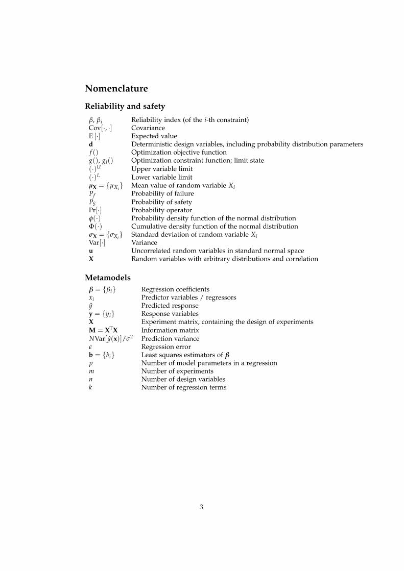
Nomenclature

Reliability and safety

β, βi Reliability index (of the i-th constraint)Cov[·, ·] CovarianceE [·] Expected valued Deterministic design variables, including probability distribution parametersf () Optimization objective functiong(), gi() Optimization constraint function; limit state(·)U Upper variable limit(·)L Lower variable limitµX = µXi Mean value of random variable XiPf Probability of failurePS Probability of safetyPr[·] Probability operatorφ(·) Probability density function of the normal distributionΦ(·) Cumulative density function of the normal distributionσX = σXi Standard deviation of random variable XiVar[·] Varianceu Uncorrelated random variables in standard normal spaceX Random variables with arbitrary distributions and correlation

Metamodelsβ = βi Regression coefficientsxi Predictor variables / regressorsy Predicted responsey = yi Response variablesX Experiment matrix, containing the design of experimentsM = XTX Information matrixNVar[y(x)]/σ2 Prediction varianceε Regression errorb = bi Least squares estimators of βp Number of model parameters in a regressionm Number of experimentsn Number of design variablesk Number of regression terms

3

1 Introduction

Reliability-Based Design Optimization (RBDO) has seen rapid developmentin the recent decades, and a number of studies which document, review andcompare the available algorithsm have appeared. Most recently, the works of(Aoues and Chateauneuf 2010) and (Valdebenito and Schuëller 2010) providea solid review of existing RBDO methods as well as an attempt to compareobjectively a selection of reviewed algorithms. A large number of methodsand approaches have been published in the recent decade, which signifies thelevel of interest in the field and its relative immaturity. Practical applicationsof RBDO methods have also been well documented, and some of the methodseven gain traction in commercial finite element analysis codes, for exampleAltair HyperStudy (Altair Engineering Inc. 2012).

None of the available RBDO methods can be considered “best in class” forall possible optimization problems. The numerical difficulties in solving theRBDO problem caused the development of many methods, each with theirunique assumptions and features.

1.1 Survey purpose and goals

This survey focuses primarily on the historical development of RBDO and thevarious classes of methods which emerged through the years. While reviewson contemporary RBDO methods have been done previously, they haven’tincorporated the basis on which such developments were possible in the firstplace — risk-based design and limit-state design. This study attempts to linkthe RBDO field with these methodologies for a more complete picture of thefield of reliability and safety.

In addition, metamodelling and particuarly its use in the context of RBDOis reviewed as well. While a number of research publications use standardmetamodels in their exposition, there are many works which attempt to tailora particular metamodel to the unique properties and features of RBDO.

While this study tries to provide a comprehensive perspective on RBDOmethods, their development and related technologies, it does not attempt tocompare various RBDO methods. Such studies have already been performedand replicated, see the aforementioned reviews by (Aoues and Chateauneuf2010) and (Valdebenito and Schuëller 2010).

1.2 Survey Structure

This study is comprised of several distinct sections which treat different as-pects of reliability, RBDO and metamodelling. In section 2, some backgroundinformation is presented on reliability and safety, as well as structural opti-mization. Section three discusses in detail reliability-based design optimizationand the development of various methods and algorithms in the field throughthe years. Section four gives an overview response surfaces and presents a fewother related metamodelling techniques. In the fifth section, the combined useof metamodels and RBDO is explored, particularly metamodels specificallyadapted for the needs of RBDO as opposed to general modelling methodspresented in the previous section. Finally, the survey concludes with a briefreview of current and anticipated future trends in the field.

4

2 Background

2.1 Reliability and safety

When talking about safety design, the concept of reliability is invariably men-tioned. (ISO 2394:1998) defines reliability as

[. . .] the ability of a structure to comply with given requirementsunder specified conditions during the intended life.

Structural engineering is one of the first disciplines which recognized theimportance of safety and reliability, due to the difference of magnitude ofinvestment, time and cost of failure compared to other engineering fields,for example mechanical engineering. Due to the varying material properties,manufacturing conditions and load uncertainties, the concept of permissiblestress design (PSD)1 was developed. In PSD, the design stresses in a structureare reduced by use of safety factors so that they do not exceed the elastic limitof materials.

The PSD design philosophy is straight-forward to understand and is ade-quate for simple load cases, but its trustworthiness is reduced when more thana few interdependent loads are used. For example, consider a simple rotatingshaft supported by two bearings. Some of the factors that can influence themaximum stress in the shaft are: variations in the elastic properties of the ma-terial, misalignment of the bearings during assembly, shaft imbalancing duringoperation, presence of stress concentrators and their severity, etc. Moreover, acombination of these factors can be present simultaneously, and a safety factorshould be associated to every possible (or at least most common) combinationof these influences. The number of necessary safety factors increases signifi-cantly for each new aspect considered, and renders this approach unusable forcomplicated load cases.

2.2 Risk-Based Design

Risk-based design is an early probabilistic approach, developed in the 1950’s,which tries to follow a probabilistic to the previously used heuristic andexperience-based method of determining safety factors. A comprehensivesummary of the risk-based design concept can be found in (Freudenthal,Garelt, and Shinozuka 1966). In risk-based design, only two variables areconsidered — the load of the structure, S, and its resistance or capacity R. Bothof these variables are assumed to be random, with given means, variances andprobability density functions (PDFs). Failure is defined as the condition inwhich the resistance of the structure is smaller than the applied load, i.e. theratio

ν =RS

(1)

is smaller than one. In terms of probability of failure, we can estimate it asfollows:

Pf = Pr(ν < 1) (2)

1In USA, PSD is more commonly called “allowable stress design” (ASD).

5

2.3 Limit State Design

Limit state design (LSD) is a design format that incorporates multiple safety fac-tors and provide a more uniform way of treating multiple load cases. LSD hasbeen introduced by various national industry standard organizations duringthe 1960’s and the 1970’s, for example under the name ultimate strength design in(ACI 318-63), partial safety factor formats (NKB 1978), load and resistance factordesign (LRFD) in USA (Ravindra and Galambos 1978), and as limit state designwhich is adopted as the design methodology of the Eurocodes (EN 1990:2002).

A central concept in LSD is limit state. (EN 1990:2002) supplies the followingdefiniton:

[. . . ] a condition beyond which a structure (or one or more of itsconstituent members) is no longer able to satisfy the provisions forwhich it was designed.

Some examples of limit states from structural mechanics are tensile failure,bending fracture, buckling, wearing, surface scratching etc. Distinction is madebetween ultimate limit states and serviceability limit states. The first appliesto conditions that cause, complete loss of load bearing ability of the structure,including structural collapse, loss of equilibrium, loss of connection betweenstructural members, buckling; as well as structural conditions that presenta risk for people’s safety. Serviceability limit states are conditions relatedto structure’s functionality, durability, usability and appearance that do notcompromise the load-bearing capacity of the structure, for example cracks,permanent deformations or vibrations (Madsen, Krenk, and N. C. Lind 1986).

Limit states are represented by mathematical models which are functionsof various load, resistance and geometric parameters. The general form of alimit state is as follows:

g(sid, rjd, lkd) > 0 (3)

where sid, rjd and lkd are the design values of the load, resistance and geometricparameters, respectively. These design values are determined from a set ofcharacteristic values which are commonly the expected (nominal) values of thecorresponding actions, and are augmented by a set of factors which take intoaccount various uncertainty sources and their severity. Load factors typicallyare greater than one to compensate for above-average loads, impact loads,wear etc., while resistance factors are commonly less than zero to account forvarying material properties and manufacturing defects.

For example, a bar loaded in tension, the stress caused by the tensile force isthe load parameter, while the allowable yield stress is the resistance parameter.The condition of tensile failure (tensile stress exceeding yield stress) is the limitstate. This can be expressed mathematically with the well-known relationship

g = σall − σt ≥ 0 (4)

In limit state design, by convention g < 0 signifies violation of the limit state,i.e. structural failure.

The basic definition can be expanded in several ways: the load and resis-tance factors can be further decomposed into additional factors that account

6

for multiple sources of uncertainty; additional load combination and impor-tance factors can be assigned to compensate for positive feedback effects frommultiple simultaneous actions; inclusion of accidental or progressive limitstates.

Drawbacks of the LSD method

The LSD method has merits for attempting to structure the existing approachesin dealing with uncertainties, however it has some significant drawbacks aswell:

Proliferation of factors While the LSD method can be efficient and straight-forward for small number of actions, the temptation to add yet another influ-ence and factor to the model can lead to unwieldy tables with a large number ofparameters. For example, (EN 1990:2002) distinguishes between three differentvariable action factors: frequent, quasi-permanent and the combination of thetwo. For buildings, the standard lists four different types of loads with differentcategories within each, giving a grand total of more than 30 possible factorvalues, depending on the load type and supplemental conditions. One can seethat, taken to the extreme, this approach ceases to be effective due to the effortrequired from the designer to navigate the requirements and determine theapplicable factors and conditions. Once the factors are determined, however,calculating the design values becomes a simple matter.

Handling of dynamic effects There is no inherent mechanism to account forthe dynamics of the structure. Dynamic actions are simply augmented withlarger load factors which do not take into account the frequency and amplitudeof the dynamic loading. This leads to systemic overdesign of the structure tocope with a worst-case scenario which can occur only in a small fraction of theproduct life cycle.

Stagnancy Once determined, the factors can continue to be used for extendedperiods of time without revision while new materials, more precise manufac-turing methods and construction techniques are introduced. Due to the purelynumerical nature of the factors which don’t have any physical relevance, ap-plying the same factors in a new set of circumstances can be cost-inefficient atbest, and life-threatening and worst.

Unquantifiable reliability When using safety factor formats, the reliabilityof the structure cannot be established accurately, since the factors are chosen insuch a way as to impart a certain predefined reliability in advance. There isno way to predict the reliability of a structure with values of its design state.Designs can easily be compared one to another, but the lack of a quantifiablereliability estimation promotes usage of higher than necessary safety factors.

7

3 Reliability-Based Design Optimization

RBDO is a natural extension of deterministic optimization. In performingthe latter, a question that often arise is how sensitive is the optimal solutionto changes in design parameters. Estimation of sensitivity is generally notpossible without performing a prohibitively costly sensitivity analysis. Instructural optmization, this often requires performing a number of additionaltime-consuming finite element simulations, which is not desireable.

The uncertainties of design parameters are not a new phenomenon, andtraditionally designers coped with them by using safety factors which are eitherprescribed in codified standards or are established internally in each companydepending on the availability of manufacturing processes and quality controlmethods. However, safety factors are rarely more than empirical rules ofthumb and it is not obvious how they should be applied to new situations andproducts without previous experience. Moreover, emprical safety factors tendto become inaccurate in time due to the development of new manufacturingtechniques and utilization of new materials.

Both over- and underdesign of machine components carry a cost for acompany — overdesign is associated with higher manufacturing and operatingcosts, while underdesign can cause significant raise in service costs and canhave immeasureable operational safety implications.

The reliability-based design optimization methods attempt to include theinherent variability of design parameters into the optimization process itself,thus providing a more

Comprehensive studies on RBDO methods (Aoues and Chateauneuf 2010),(Valdebenito and Schuëller 2010) divide RBDO methods into three categoriesdepending on the methods’ structure: double-loop, single-loop approach anddecoupled approaches.

3.1 General RBDO formulation

The basic problem of RBDO is posed as a minimization of an objective functionunder probabilistic and also possibly deterministic constraints.

minX

E [ f (X)]

s.t. Pr[gi(X) ≤ 0] ≥ PSi, i = 1, . . . , m(5)

where X is a vector of random variables with known distributions, gi(X)denotes a set of constraints, each with a prescribed probability of safety PSi.Deterministic constraints and variables can also be treated without specialarrangements, but for simplicity they will not be considered in this text.

The presence of the probabilistic constraint precludes use of traditionalgradient-based methods.

The actual probability of failure of the structure is given by integrating overthe failure region:

Pr[gi(X > 0)] =∫· · ·

∫gi(X)>0

fX(x)dx1dx2 . . . dxn, i = 1, . . . , m (6)

8

Here, fX is the joint probability density function (JPDF) of all design parametersin x. The evaluation of this integral is comppounded by two factors: forpractical problems, the JPDF is either unknown or very difficult to estimate,especially for interdependent variables; the multi-dimensional nature of theintegral makes its numerical computation challenging. To overcome thesedifficulties, analytical approximations of first and second order have beenproposed.

The probability constraint in (5) can also be evaluated using the MonteCarlo method (Metropolis and Ulam 1949). The Monte Carlo method involvesgenerating a large number of sampling data and estimating the probabilitybased on these samples. This is typically considered a heavy-handed, brute-force approach, due to the significant computational effort required. In orderto guarantee sufficiently good accuracy and minimize sampling error, a largenumber of experiments need to be performed. For example, probabilitiesof the order of 99% i.e. failure rate of 1% would require a few hundredsamples to establish reasonable bounds on the sample probability, while formore practical reliability levels with failure rates of 0.01% or lower, tens ofthousands of sample points are necessary. Additionally, sufficiently accuratemodelling of non-uniform probability distributions of the design variables isrequired to guarantee that each sample set conforms to the desired distributionparameters, which complicates the random number screening procedure. Whenfinite element analysis is used to provide experimental data, a Monte Carlosimulation becomes extremely time-consuming and practically infeasible.

The reliability estimation is only a part, albeit crucial, of the RBDO problem.Accurate reliability estimation is central to the development of successfulreliability-based design optimization algorithms.

3.2 Early Developments

One of the first major advances in reliability theory was the idea of (Cornell1969) to express all uncertainties of the random variables only in terms of theirfirst and second moments (means and covariances). The method introducesa failure function (limit state function) which divides the variable space intofailure region and safe region. A safety margin M represents the value of thefailure function at each point in the design space:

M = g(Xi) (7)

and a reliability index βC is defined as the ratio between the expected valueof the safety margin and the distance between the failure function and theexpected value of the safety margin:

βC =E[M]

D[M](8)

In the spirit of risk-based design, Cornell proposes the failure function as adifference between the resistance and the load on the system:

g(r, s) = r− s (9)

which corresponds to safety margin

M = R− S (10)

9

Using general statistical relations, formulas can be derived for uncorrelatedload and resistance variables as functions of their means and standard devia-tions. The Cornell method, while representing a novel approach to reliability,suffers from two major disadvantages: formulation of a linear safety marginis not possible if the failure function is not a hyperplane; and its arbitrarinessprecludes using the reliability index as a more universal measure of reliabilitybetween different problems, or even two different formulations of the sameproblem.

A logarithmic scaling of the load and resistance variables has been intro-duced in (Rosenblueth and Esteva 1972) to restrict the variable domain only topositive values, which allows for a more natural treatment of physical variableswithout introducing additional constraints. The safety margin becomes a non-linear function in this case, which requires the use of a linearization procedure.This formulation circumvents some of the drawbacks of the reliability indexdefined by Cornell, but the question of arbitrariness of the failure function stillremains, further compounded by the arbitrariness in selecting the linearizationpoint.

For a general limit state as a function of many random variables, a first-order approximation around the mean point can be written as

g(X) ≈ g(X) = g(µX) +n

∑i=1

∂g∂Xi

(Xi − µXi )

+12

n

∑i=1

n

∑j=1

∂2g∂Xi∂Xj

(Xi − µXi )(Xj − µXj) + · · ·(11)

If we collect only the linear terms, we can estimate the first-order approximatemean and variance of the limit state function as

µg ≈ g(µX1 , µX2 , . . . , µXn)

σ2g ≈

n

∑i=1

n

∑j=1

∂g∂Xi

∂g∂Xj

Cov(Xi, Xj)(12)

This is possible due to the properties of the normal distribution — linearcombinations of normally distributed variables are also normally distributed,and their means and variances are calculated as shown above. For uncorrelatedvariables, the standard deviation is simply

σg ≈

√√√√ n

∑i=1

(∂g∂Xi

)2σ2

Xi(13)

where β is the reliability index of the design and is calculated as the ratiobetween the mean and the standard deviation of the limit state:

β =µg

σg(14)

The corresponding probability constraint is then estimated as follows:

Pr[g(X ≤ 0)] ≈ Φ(

0− µg

σg

)= Φ(β) (15)

10

This approximation of the probability of failure using only first-order informa-tion as well as the first and second moments of the probability distributionsof the design avariables is known as first-order reliability method (FORM). Ifthe Taylor expansion is performed around the mean point of the limit state,the method bears the name mean value first-order second-moment method(MVFOSM). A significant drawback of MVFOSM is that no information onthe actual distribution of the random variables is used. For linear limit states,the estimated reliability is accurate, but for non-linear failure functions theomission of high-order terms can introduce a significant error.

The first-order approximations of the probability of failure in (15) is onlyappropriate when the limit state is linear or close to linear in the region ofthe current design point: general non-linear limit states cannot be modelledappropriately using only linear terms. Approximations which incorporatesecond-order information, called second-order reliability method (SORM),were first investigated by (Fiessler, Neumann, and R. Rackwitz 1979). Aclosed-form solution was later provided by (Breitung 1984), as follows:

Pr[g(X ≤ 0)] ≈ Φ(β)n−1

∏i=1

1√1 + 2βκi

(16)

where κi are the principal curvatures of the limit state at the MPP, and β is thefirst-order reliability index obtained using FORM. The principal curvatures areobtained by first performing an affine rotation around the origin of the designspace, so that it coincides with the gradient vector α of the limit state at theMPP. The rotation matrix R is calculated by orthonormalising of the matrix R0,defined as:

R0 =

1 0 · · · 00 1 · · · 0...

.... . .

...α1 α2 · · · αn

(17)

The principal curvatures are the eigenvalues of the matrix A, whose elements aijare computed as

aij =(RGRT)ij

||∇g(z∗)| | , i = 1, . . . , n− 1

G = ∇2g(z∗)

(18)

The Breitung approximation includes only parabolic terms — mixed second-order terms and their derivatives are ignored. SORM estimates using thisformula are generally only accurate for high target reliability. An alternativeformulation has been proposed by (Hohenbichler et al. 1987), as follows:

Pr[g(X ≤ 0)] ≈ Φ(β)

n−1

∏i=1

1√1 + 2 Φ(β)

Φ(−β)κi

(19)

Another method is proposed by (Tvedt 1990) which uses both parabolic and asecond-order approximation of the limit state, but without using asymptoticapproximations. This method circumvents the low accuracy of the Breitungformula at low reliability levels, while still remaining accurate at high targetreliabilities.

11

3.2.1 Hasofer-Lind Reliability index

THasofer and Lind (1974) introduced a method that builds on the ideas ofCornell, particularly the use of the reliability index and the first and secondmoments only to estimate the reliability. An important feature of the proposedreliability criterion is the invariance of the reliability index under equivalenttransformations of the design variables. Hasofer and Lind introduce a nonho-mogenous linear mapping between the original set of random variables Xi ontoa new set Zi of normalized and uncorrelated variables. Formally, this meansthat the expected values of the new variables are zero, and the covariancematrix is the unit matrix:

E [Z] = 0

Cov(Z, ZT) = I

In the newly-constructed design space of variables Zi, the geometrical distancebetween the origin and the transformed failure surface g(Z) corresponds tothe distance (in standard deviation units) from the mean point in x-space tog(X). In other words,

βHL(z) =√

zTz (20)

For normal variables, this is readily achieved by transforming the variablesinto standard normal form with zero mean and unity standard deviation:

Zi =Xi − µXi

σXi

, i = 1, . . . , n (21)

For other distributions, however, such transformations are not possible, whichputs a severe restriction on the method’s applicability. Still, near-equivalenttransformations to normally distributed uncorrelated variables are possible, forexample the two-parameter equivalent normal transformation due to Rackwitzand Fiessler (1976). With this transformation, the cumulative distributionfunction (CDF) and the PDF are made equal at the design point on the failuresurface. While appropriate for symmetric distributions, the Rackwitz-Fiesslermethod is increasingly inaccurate for highly-skewed distributions such asextreme value distributions like Gumbel, Frèchet or Weibull.

The point on the failure surface which corresponds to the reliability indexis called design point or most probable point (MPP). When the failure surface isa hyperplane, the reliability indices of Cornell and Hasofer-Lind coincide. TheMPP can be selected as a linearization point, and this approach is commonlyknown as advanced first-order second-moment method (AFOSM) in literature.

3.2.2 Finding the Most Probable Point

Using equation (20), the most probable point is the point on the failure surfaceclosest to the origin in the reduced coordinates. Formally, this corresponds tosolving the following optimization problem:

minz

√zTz

s.t. g(z) = 0(22)

12

Initially, an iterative algorithm was devised for solving such problems, dueto Rackwitz and Fiessler (1978), later expanded by Ditlevsen (1981) to coverdependent variables. The algorithm is simple to implement and understand,and it uses first-order derivative information to calculate the point of nextiteration. However, its convergence is not guaranteed, and standard constrainedoptimization algorithms can be successfully used instead.

3.2.3 Transformation in standard normal space

The Hasofer-Lind reliability index is defined only for normally distributeddesign variables; the transformation to standard normal space is not validfor other probability distributions. The Rosenblatt transformation (Rosenblatt1952) can be used to obtain a set of uncorrelated variables with standard normaldistribution, provided that the joint CDF of all original design variables isavailable.

Alternative methods, such as Rackwitz-fiessler method (Rüdiger Rackwitzand Fiessler 1976), can be used to provide a two-parameter equivalent transfor-mation into standard normal variables. With this algorithm, the CDF and thePDF at the current design point x∗ = x∗i should be equivalent in the actualand the normalized variables:

Φ

(x∗i − µN

Xi

σNXi

)= FXi (x∗i ), i = 1, . . . , n (23)

which results in the following expressions for the mean and standard deviationof the normalized variables:

µNXi

= x∗i −Φ−1 (FXi (x∗i ))

σNXi

σNXi

=φ(Φ−1 (FXi (x∗i )

))fXi (x∗i )

(24)

This transformation is fairly accurate for close-to-symmetric probability dis-tributions, but the estimates of the mean and standard deviation are oftennot satisfactory for highly skewed or naturally bounded distributions, such asFréchet or beta distributions. Extensions of the Rackwitz-Fiessler algorithmhave also been published, for example the three-parameter transformationdue to Chen-Lind (X. Chen and N. Lind 1982), which in addition to the meanand standard deviation also uses a scale factor that equates the slopes of theoriginal and the transformed distributions at the design point.

3.3 Double-loop approaches

Nikolaidis and Burdisso (1988) utilized the idea of Hasofer and Lind and pro-posed an iterative nested optimization procedure to solve the RBDO problem asstated in (5). The inner optimization loop estimates the reliability at the currentsolution, while the outer loop optimizes the overall cost function using thereliability calculated in the inner loop. The authors used both MVFOSM andAFOSM for reliability assessment in the inner loop and ultimately concludedthat the latter is more accurate and robust. This approach is commonly referredin the literature as reliability index approach (RIA).

13

The reliability index method, while capable of solving the RBDO problem,was later found to be slowly convergent, numerically unstable and compu-tationally expensive, especially at high reliability levels. Tu and Choi (1999)introduced the performance measure approach (PMA) which performs in-verse reliability analysis, under the assumption that it is simpler to optimize acomplex function with simple constraints than vice versa.

The method is shown to be more robust and efficient in a comparativestudy performed by (J.-O. Lee, Y.-S. Yang, and Ruy 2002). The main differencebetween RIA and PMA is the formulation of the MPP problem. While in RIAthe MPP is found by minimizing the distance to the failure surface, in PMAthe objective and the constraint have been interchanged:

minz

g(z)

s.t. ||z|| = βa(25)

The constraint always has the shape of a hypersphere, which simplifies signifi-cantly the optimization problem as specialized algorithms for solving them aredevised.

3.4 Single-loop approaches

Double-loop approaches require significant computational effort due to thenested optimization and probabilistic loops, and efforts to increase the perfor-mance of RBDO algorithms lead to the work of (Xiaoguang Chen, Hasselman,and Neill 1997), which replaces the probabilistic constraints with approximatedeterministic ones. Thus, the inner probabilistic loop is eliminated, result-ing in a more efficient algorithm. This method is known in the literature assingle-loop, single-vector approach (SLSV). A similar work has been publishedpreviously by (Thanedar and Kodiyalam 1992). However, the method wasshown to be inadequate for non-linear problems due to the linear assumptionof FORM (R. Yang and Gu 2004).

Single-loop approaches based on Karush-Kuhn Tucker conditions (KKT)Parallel to the development of SLSV, (Madsen and Hansen 1992), and laterimprovements by (Kuschel and Rüdiger Rackwitz 1997), approached the prob-lem from a different perspective — the reliability analysis is replaced by thecorresponding KKT optimality conditions, thus allowing the use of standardoptimization algorithms. Two formulations of RBDO problems are suggested,which differ somewhat from the problems typically studied: total cost min-imization (CRP) and reliability maximization (RCP). The CRP has a generalformulation as follows:

minu

Ct(p) = Ci(p) + C f (p)Φ(−∥∥u∥∥)

s.t.

g(u, p) = 0uT∇ug(u, p) +

∥∥u∥∥ · ∥∥∇ug(u, p)

∥∥ = 0

(26)

where Ct, Ci C f are the total, initial and failure cost respectively; u is a transfor-mation of the original vector X of random variables into uncorrelated variableswith standard normal distribution, and p is a vector of deterministic variables

14

and distribution parameters. Additional constraints on the design parameterscan also be specified as necessary.

While the method does away with the inner optimization loop, it requirescalculation of second-order derivatives of the constraints, which can be compu-tationally costly and inaccurate. Only FORM assumption of the probability offailure is made, with authors claiming that expansion to second-order reliabil-ity method can be problematic. The probabilistic transformation from X to uneeds to be specified explicitly, with its associated approximation errors.

However, the probabilistic transformation need to be specified explicitly,and while only first-order optimality conditions are used, second-order deriva-tives of the constraints are required as well. The authors also observe sensitivityto initial values, and the necessity of monotonic transformation of the objectiveand the constraints to improve convergence.

This work is later extended in (Kuschel and Rüdiger Rackwitz 2000) tosolve optimization problems with time-variant constraints, although underthe assumption of Poisson failure process and limited to first-order reliabilityestimation.

In a related paper, (Agarwal et al. 2007) applied the same first-order KKTnecessary conditions, but this time replacing the RIA-formulated reliability loopused in (Kuschel and Rüdiger Rackwitz 2000) with PMA. The authors observeimproved computational efficiency and robustness compared to double-loopapproaches.

Improvements to the SLSV were suggested in (Liang, Mourelatos, andNikolaidis 2007), which relates the approximations to the KKT conditions ofthe inverse FORM. The suggested optimization problem to solve looks like

minµX

f (µX)

s.t. gi(xki ) ≤ 0, i = 1, . . . , m

where

xk

i = µkX − αk

i σXβTi

αki =

σX∇gi(xk−1i )∥∥∥σX∇gi(xk−1i )

∥∥∥σX = σXi

(27)

This approach is commonly referred to as single-loop approach (SLA). NoMPPs are calculated in this formulation — by solving the KKT conditions,an approximation of the MPPs of the active constraints is used. The KKTconditions involve the normalized sensitivities αi which are approximate bythe MPP estimate from the previous iteration. One of tha major differenceswith the approach of (Xiaoguang Chen, Hasselman, and Neill 1997) is that thenormalized sensitivities are calculated exactly instead of being approximatedor assumed.

The authors recognize a drawback of SLA, particularly problems withconverging to the global optimum, if the limit states are very non-linear. Sincethis approach uses approximations of MPPs instead of actually calculatingthem, it is more sensitive to non-linearities than double-loop methods.

Another method that can be classified as single-loop approach is the proce-dure outlined in (Shan and G. G. Wang 2008). In contrast to other methods,this algorithm first determines a reliable design space in which the reliability

15

constraints are enforced throughout, and subsequently performs a determin-istic optimization within this constrained space. The gradients at the currentsolution are used as approximation for the gradients at the MPP, thus eliminat-ing the reliability analysis altogether. This has the advantage of not needing aspecialized optimization algorithm which embeds reliability analysis, and stan-dart deterministic optimization methods can be used instead. The approach isshown to work for a set of known analytical benchmarks, however its accuracycan be suboptimal for very non-linear problems.

3.5 Decoupled approaches

Reliability analysis has proven to be the bottleneck of most RBDO methods, andwhich spurred the development of a class of methods that avoid performingreliability analysis at each step of the optimization. Those methods are com-monly referred to as decoupling approaches. A key feature of all decouplingapproaches is the deterministic approximation of the reliability index.

Sequential optimization and reliability assessment (SORA), introduced in(Xiaoping Du and Wei Chen 2004), performs reliability analysis and determinis-tic optimization in two alternating cycles in each optimization step. In the firstcycle, the deterministic solution of the optimization problem is first obtained,using standard optimization procedures. Since the reliability requirements ofmost constraints will be likely violated, in the second cycle they are shiftedinto the probabilistic feasible region by means of a shifting vector

s = µX − xMPP (28)

The inverse MPPs of the constraints are calculated after the second cycle usingthe method of (Tu, Kyung K. Choi, and Park 1999), and since the feasible spacehas been reduced, the reliabilities of the violated constraints are expected toimprove. The method formulation can be more formally expressed as follows:

minµX

f (d, µX)

s.t. g(d, ux − s) ≤ 0(29)

The two cycles are repeated until the objective converges and the shiftingdistances become zero, i.e. the reliability requirements are satisfied. In thisformulation, the design variables are assumed to be normally distributed anduncorrelated, however arbitrary distributions can be used provided that atransformation to standard normal random variables is available.

An extension of SORA has been suggested by (Cho and B. Lee 2010), usingmethod of moving asymptotes (MMA) and convex linearization (CONLIN)approximations instead of linear Taylor expansion. CONLIN, developed by(Fleury and Braibant 1986), and MMA, first presented by (Svanberg 1987) andfurther extended in (Svanberg 2002), are adaptive approximation schemeswhich can utilize the specific structure of the problem and linearize the ob-jectives and constraints with respect to the reciprocals of the design variables.Cho et al. tested the method on various types of problem and its accuracy andnumerical performance match or exceed those of SORA.

16

Approximating reliability index A class of decoupled approaches forego thereliability analysis altogether by utilizing an approximation of the reliabilityindex. An early attempt in this direction can be found in (Royset, Kiureghian,and Polak 2001), where the reliability index is replaced by its approximationusing deterministic functions.

This class of methods utilize a direct constraint on the reliability indexrather than a probabilistic constraint:

mind

f (d)

s.t.

βt ≤ β(d)dL ≤ d ≤ dU

(30)

(Chandu and Grandhi 1995) proposed a first-order approximation of the relia-bility index based on linear Taylor expansion:

βk(d) ≈ β(dk−1) + (∇β(dk−1))T(d− dk−1) (31)

where the sensitivities of the reliability index are calculated according to (L.Wang, Grandhi, and Hopkins 1995). However, this method of approximat-ing the reliability index is not very efficient and holds little advantage overtraditional double-loop methods. (Cheng, Xu, and Jiang 2006) proposed asequential approximate programming (SAP) strategy which provides an ap-proximation of the reliability index and its gradient derived from the necessaryKKT conditions:

βk(d) ≈ β(dk−1) + (∇β(dk−1))T(d− dk−1)

λk−1 =1∥∥∇ug(dk−1, uk−1)

∥∥β(dk−1) = λk−1

(g(dk−1, uk−1)− (uk−1)

T∇ug(dk−1, uk−1))

uk = −β(dk−1)λk−1∇ug(dk−1, uk−1)

(32)

A similar approach using an active set strategy has been proposed by (Zou andMahadevan 2006).

A sequential linear programming approach has been suggested by (Chan,Skerlos, and Papalambros 2007). At each iteration, a new step s is calculatedwithin a trust region, which is used to obtain the new design point

µk+1X = µk

X + s (33)

The constraints can be approximated using either FORM or SORM assumptions;in case of FORM, the LP subproblem has the form

minsk

f T(µkX) · sk

s.t.

gk(xkMPP) +

(∇gk(xk

MPP))T· sk ≤ 0∥∥∥sk

∥∥∥ ≤ ∆k

where xkMPP = µk

X + σXβt∇gj∥∥∇gj

∥∥(34)

17

The MPPs are derived using KKT conditions in a similar fashion as in (Liang,Mourelatos, and Nikolaidis 2007). SORM-based SLP uses the principal curva-tures κ to estimate the reliability index.

3.6 Comparative studies

There is no shortage of RBDO methods developed in the last decade, andwhile there have been attempts to categorize and compare different approachesto find the “best” one, there is currently no method that is recognized assuperior in all situations. The main reason for this is that RBDO methodsare often developed to solve a particular type of problems, factoring numberand distributions of design variables, linearity of the problem, system vs.component reliability, static vs. stochastic loading, large or small numberof limit states, etc. Direct, objective comparison between methods is thusproblematic. Still, a number of studies attempted independent tests of variousRBDO approaches. (R. Yang and Gu 2004) provided an early study comparingSORA and SLSV to double-loop approaches for a variety of analytical andstructural optimization problems. In this study, SORA and SLSV consistentlyshowed superior performance and accuracy compared to traditional double-loop methods.

In recent years, (Aoues and Chateauneuf 2010) provided a comparisonbetween the most well-known methods currently in use, including RIA, PMA,KKT-based methods, SLA, SORA and SAP. A variety of problems with distinctcharacteristics were shown. SLA, SORA and SAP show overall good perfor-mance and accuracy for problems with nonlinear limit states, large numberof design variables and non-normally distributed random parameters. Othermethods were shown to perform more favourably in certain situations — KKTconverges quickly for problems with small number of variables and constraints,but can be numerically unstable and inefficient for problems with non-normallydistributed variables; PMA and RIA have adequate efficiency when limit statesensitivities are given analytically, and work well with variables with non-Gaussian distribution, but are generally the slowes, sometimes by a factor ofthree or more.

Another comprehensive study comparing various methods that appearedrecently is due to (Valdebenito and Schuëller 2010). The authors assert thatobjective testing of RBDO algorithms is problematic and instead discuss variousaspects which differentiate the methods, such as dimensionality of the designvariables and uncertain parameters, application of meta-modelling, componentvs. system reliability.

18

4 Metamodels

Computer models of various processes have been used extensively in the lastfew decades — for example, finite element simulations, climate models, molec-ular models, etc. Such abstractions have proven their accuracy in predictionof the properties of the observed process, however obtaining results fromutilizing these models can be time-consuming and computationally intensive.For instance, a typical finite element simulation in industrial setting can runfrom an hour to a week — clearly undesirable situation if a large number ofsimulations need to be carried out. For this reason, metamodels (i.e. “mod-els of models”) have been developed. Metamodels (also referred sometimesas “surrogate models”) are not phenomenological, but purely mechanistic —instead of simulating the actual physical process, they mimic its behaviourin a limited domain, for which they have been deemed sufficiently accurate.Metamodels are typically very fast to evaluate, and are a valuable tool when alarge number of results are desired. Process optimization also benefits greatlyfrom using metamodels.

Response surface method (RSM) is a popular metamodelling technique.According to (Roux, Stander, and Haftka 1998), response surface methodologyis defined as

. . . a method for constructing global approximations to system be-haviour based on results calculated at various points in the designspace.

Response surfaces are constructed using a predefined set of data points (adesign of experiments) within the range of all variables of interest, and aregression model is fitted to the data points. The DoE and the chosen regressionmodel are critical to achieving good model accuracy and predicting capabilitiesin the unsampled portions of the design domain.

Regression models of various complexity and structure are at the heart ofRSM. The simplest such model is a linear regression of multiple variables, asshown below:

y = β0 +k

∑j=1

β jxj + ε (35)

Here, ε is the regression error term with assumed E(ε) = 0 and Var(ε) = σ2,and uncorrelated components.

Given m observations, we can write an expression for each experimentusing (35):

yi = β0 +k

∑j=1

β jxij + εi, i = 1, . . . , m (36)

19

We can write (36) in matrix form as follows,:

y = Xβ + ε

y =

y1y2...

ym

, X =

1 x11 x12 · · · x1k1 x21 x22 · · · x2k...

......

...1 xm1 xm2 · · · xmk

β =

β1β2...

βk

, ε =

ε1ε2...

εm

(37)

Minimizing the deviation of the regression model from the actual responseat the design points is equivalent to minimizing εi in the least squares sense.The least squares estimator of β and the fitted regression model can then beexpressed by

b = (XTX)−1XTyy = Xb

(38)

The least squares estimator is unbiased — its expected value is equal to theregression coefficients β. The covariance of b can be expressed as

Cov(b) = σ2(XTX)−1 (39)

where an unbiased estimator of σ2 is given by

σ2 =SSE

m− k=

m

∑i=1

(yi − yi)2

m− k(40)

Quadratic and higher-order models are also used, however the increasednumber of interactions between variables requires more regression coefficientsto be calculated and more experiments to create an adequate model.

A comprehensive historical perspective of the development of RSM can befound in (Myers, Khuri, and Carter Jr. 1989). An excellent introduction to RSMand DoE can be found in (Myers and Montgomery 2002).

4.1 Design of experiments

One of the most important elements that influence the accuracy and efficiencyof the regression model is how the design points are selected in the feasibledesign space. Important considerations when building response surface modelsare coverage and size, as the number of experiments one is allowed to performis typically constrained by cost and/or available time. From time and costperspective, it is advantageous to minimize the number of experiments —physical tests require significant effort to set up and execute, and a singlenumerical simulation of a large model can easily take from one hour to oneweek or more wall clock time. However, large samples allow building morecomplex and accurate models, and have generally better predictive capabilitiesthan smaller smaples.

20

Effcient designs of experiments have a number of desirable properties thataffect their accuracy and prediction power:

• Prediction variance. The variance of a predicted response is given by

Var[y(x)] = ξxT(XTX)−1ξ(x) · σ2 (41)

where ξ(x) is the selected basis of the model as a function of the designpoints. This makes the prediction variance an explicit function of theselected experimental design.

The scaled prediction variance is useful when comparing various sam-pling schemes, as it is dimensionless:

v(x) =NVar[y(x)]

σ2 (42)

A stable prediction variance (rather, its scaled version) is preferablefeature of experimental designs, as it provides assurance that predictedresponses would be similarly accurate regardless of the position of themeasured point in the design space.

• Orthogonality. For a design to be orthogonal, the scalar product of anytwo column vectors in the design must evaluate to zero; in other words,the information matrix XTX becomes diagonal. This minimizes predictionvariance over the regression coefficients when using linear regressions.

• Rotatability. The concept of rotatability is introduced in (Box and Hunter1957) and refer to a design for which the prediction variance is constantat any point situated at the same distance from the design center. Thus,spherical designs are inherently rotatable and thus preferable.

Rule-based designs Factorial designs are simple and straight-forward toimplement — a few (two or three are most common) levels of each variablesare selected, and a DoE capturing all possible combinations between all levelsof design variables are created. This type of designs is suitable for screeningexperiments to identify the most important variables in the modelled process. 2k

designs are suitable for fitting a first-order model, and are often the basis formore complex experiment setups.

While adequate for small number of variables, the number of experimentsgrow exponentially with number of variables: the number of necessary designpoints m can be calculated using the expression

m =n

∏i=1

li (43)

where li is the number of levels for each design variable and n is the numberof design variables. For example, a 2k design of ten variables, each with twolevels, would require 1024 experiments, which often is prohibitively expensiveand time-consuming for practical problems. For this reason, more compactdesigns of experiments have been devised through the years that scale betterwith increasing the number of variables.

21

One instance where factorial designs of low order are particularly valuableis screening experiments — eliminating factors with negligible effect on theresponse. This allows exclusion of the associated design variables from fur-ther investigations, which yields simpler and faster to construct and evaluatemetamodels.

Central composite designs (CCDs), introduced in (Box and Wilson 1951),is a sequential scheme which combines a full two-level factorial designs withaxial and central runs to create a spherical coverage of the design domain.According to (Myers and Montgomery 2002, p. 321), this design is one of themost used second-order schemes. The rationale for this kind of design is toprovide a stable prediction variance through the use of factorial design, and atthe same time give information about coupling effects between variables. Anexample CCD matrix for three design variables is shown below:

D =

−1 −1 −1−1 −1 1−1 1 −1−1 1 1

1 −1 −11 −1 11 1 −11 1 1−α 0 0

α 0 00 −α 00 α 00 0 −α0 0 α0 0 0

(44)

The model has an adjustable parameter, α, which controls the extents of theaxial runs. α is commonly set to achieve spherical, thus rotatable design.

Face-centered designs (FCDs) are similar to CCD, with the design spanninga cube rather than a sphere, i.e. the parameter α is set to unity. These areapplicable when the design variables have strict upper and lower limits.

Box-Behnken designs (BBDs), due to (Box and Behnken 1960), featurethree levels of the design variables and are suitable for fitting second-orderresponse surfaces. Box-Behnken designs explore all possible combinations ofthe extremes of the design variables, taken two at a time, while the remainingvariables are set at their mid-level. A Box-Behnken design of three normalized

22

variables is given below:

D =

−1 −1 0−1 1 0

1 −1 01 1 0−1 0 −1−1 0 1

1 0 −11 0 10 −1 −10 −1 10 1 −10 1 10 0 0

(45)

BBDs occupy spherical region of interest, and as such, the scaled predictionvariance NVar[y(x)]/σ2 is constant. This is a desirable feature of sphericaldesigns, as it provides some assurance of how good y(x) is as a responseprediction. However, if the corners of the design space are of interest, BBD isnot an appropriate choice, as there are no runs that cover all variables at theirextremes.

Compact designs A class of compact designs are also available, for situationswhere every experiment counts — these designs feature adequate coverage ofthe design domain, but with reduced density and prediction accuracy.

Small composite designs (SCDs) are a variation of CCD, but without a fullfactorial design. Augmented and central runs are used in the same fashionas in CCD. A symmetry in selecting which 2k runs to include in the design isdesirable to stabilize the prediction variance. A compelling feature of SCD isthe possibility for sequential experimentation — after the factorial part of thedesign is executed, the remaining runs can be foregone if a linear model is asufficiently good fit.

Koshal designs, presented in (Koshal 1933), examine the response of thedesign variables taken only one at a time. This leads to a compact design, butwith limited possibilities of estimating interaction terms.

First-order Koshal designs follow the structure below:

D =

0 0 · · · 01 0 · · · 00 1 · · · 0...

......

0 0 · · · 1

(46)

Hybrid designs (Roquemore 1976) combine central composite designs of re-duced order with levels of the remaining variable selected in a way thatproduces near-rotatable and near-orthogonal design. The number of experi-ments is close to the minimum required to establish the desired model. Whileefficient, these designs are nearly saturated, which leaves little room for com-pensating for lack of fit of the chosen regression model. Another drawback

23

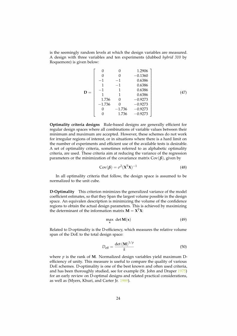
is the seemingly random levels at which the design variables are measured.A design with three variables and ten experiments (dubbed hybrid 310 byRoquemore) is given below:

D =

0 0 1.29060 0 −0.1360−1 −1 0.6386

1 −1 0.6386−1 1 0.6386

1 1 0.63861.736 0 −0.9273−1.736 0 −0.9273

0 −1.736 −0.92730 1.736 −0.9273

(47)

Optimality criteria designs Rule-based designs are generally efficient forregular design spaces where all combinations of variable values between theirminimum and maximum are accepted. However, these schemes do not workfor irregular regions of interest, or in situations where there is a hard limit onthe number of experiments and efficient use of the available tests is desirable.A set of optimality criteria, sometimes referred to as alphabetic optimalitycriteria, are used. These criteria aim at reducing the variance of the regressionparameters or the minimization of the covariance matrix Cov(β), given by

Cov(β) = σ2(XTX)−1 (48)

In all optimality criteria that follow, the design space is assumed to benormalized to the unit cube.

D-Optimality This criterion minimizes the generalized variance of the modelcoefficient estimates, so that they Span the largest volume possible in the designspace. An equivalen description is minimizing the volume of the confidenceregions to obtain the actual design parameters. This is achieved by maximizingthe determinant of the information matrix M = XTX:

maxx

det M(x) (49)

Related to D-optimality is the D-efficiency, which measures the relative volumespan of the DoE to the total design space:

Deff =det (M)1/p

k(50)

where p is the rank of M. Normalized design variables yield maximum D-efficiency of unity. This measure is useful to compare the quality of variousDoE schemes. D-optimality is one of the best known and often used criteria,and has been thoroughly studied, see for example (St. John and Draper 1975)for an early review on D-optimal designs and related practical considerations,as well as (Myers, Khuri, and Carter Jr. 1989).

24

D-optimal designs inherenhtly depend on the type of regression modelused, and are prone to biasing if inadequate regression models are used; ad-ditinoally, have the tendency to have repeated experiments at exactly the samedesign points, especially for non-regular design domains. The latter issue isparticularly problematic — while repeated trials are acceptable for physicaltesting situations, such experiments are wasteful in cases of fully deterministicnumerical simulations. A Bayesian modification has been proposed by (Du-Mouchel and B. Jones 1994) and recently investigated by (Magnus Hofwingand Niclas Strömberg 2009), which adds higher-order terms to the regressionmodel to reduce occurence of duplicates. As D-optimality is a highly non-linearproblem, algorithms to construct D-optimal designs do not converge to theglobal optimums. Search strategies based on simulated annealing and geneticalgorithms have been successfully applied, see for example (Broudiscou, Leardi,and Phan-Tan-Luu 1996).

A-Optimality Minimize the average variance of the model coefficient esti-mates without taking into consideration covariances among regression coef-ficients — that is, only the trace of the information matrix M is considered.Formally, A-optimality is defined as

minx

tr[M(x)]−1 (51)

S-Optimality S-optimal designs maximize the geomatric mean of the dis-tances between nearest neighbours of the design points:

maxx

n

∑i=1

min |xi − xj|

n(52)

Unlike other optimality criteria, S-optimal designs are independent on theassumed regression model. S-optimal designs inherently do not produceduplicates, however finding the global optimum or even a satisfactory solutioncan be difficult due to the presence of multiple local optima. (Magnus Hofwingand Niclas Strömberg 2009) applied a hybrid genetic algorithm together withsequential linear programming (SLP) to find S-optimal designs in irregulardesign domains.

I-Optimality Minimize the average of the expected variance (taken as anintegral) over the region of prediction:

minx

1K

∫Ω

fT(x)M−1f(x)w(x)dx, K =∫Ω

dx (53)

where f(x) is a row from the design matrix X and w(x) is a weighting function.This formulation is equivalent toe the following optimization problem:

minx

tr[M−1B], B =1K

∫Ω

f(x)fT(x)w(x)dx (54)

25

Given the trace operator and the integral in the definition above, direct applica-tion of standard optimization packages is difficult. Zeroth order optimizationalgorithms, for example simulated annealing in (Haines 1987), are commonlyapplied.

Prediction variance criteria A class of optimality criteria focus on measuresdirectly related to controlling the prediction variance by limiting its maximumor average over the whole design domain, a part of it, or only using a subset ofthe available design points.

G-Optimality G-optimal designs minimizes the maximum prediction vari-ance is minimized:

minζ

[maxv∈R

v(x)]

(55)

V-Optimality In V-optimality, the goal is to minimize the average predictionvariance over a set of points of interest, which may not necessarily be thedesign points used to construct the response surface.

Q-Optimality In similar vein to V-optimality, Q-optimal designs minimizethe average prediction variance, but instead of performing this on the wholedesign space, a region of interest R is used instead. The Q-optimal design isgiven by

minx

1K

∫R

v(x)dx, K =∫R

dx (56)

Space-filling designs As an alternative to alphabetical optimality criteria,other heuristic sampling-based methods can be used. Latin hypercube sam-pling (LHS) is a popular choice as it could be both efficient and easy to construct,as evidenced by a comparison study between random, stratified and Latinhypercube sampling found in (McKay, Beckman, and Conover 1979) which firstintroduced the concept. LHS designs show less estimate variance compared tosimple random sampling, as detailed in (Stein 1987). Multiple LHS-conformantdesigns can exist for the majority of problems, and choosing an “optimal”among those has been the goal of multiple studies: (Palmer and Tsui 2001)presented a LHS scheme which minimizes the integrated square basis over theregion of interest; (Morris and Mitchell 1995) describe a maximin-optimizedLHS which maximizes the minimum distance between neighbour points in theDoE; (Tang 1993) utilize orthogonal arrays to control the distribution of pointsin the design domain.

4.2 Extensions of RSM

The basic response surface method is a powerful modelling tool which hasproven its usefulness in a number of practical applications. However, is isnot always accurate or reliable enough for very non-linear problems. Severalmethods have emerged as extensions to RSM, notably Kriging method, radialbasis functions (RBFs) and successive response surface method (SRSM).

26

4.2.1 Kriging

The method was suggested originally by Danie Krige in his Master thesis (Krige1951) and further developed by (Matheron 1963). While these works providerigorous derivation of the method, a more gentle introduction to Kriging canbe found in e.g. (D. R. Jones 2001). The Kriging predictor is unbiased, basedon minimum expected squared prediction error and is a linear combination ofthe measured responses.

The regression is modelled as a realization of a stochastic process, byestimating the uncertainty of the value of the function at an arbitrary point.A mean µ and variance σ2, can be ascribed to this uncertainty, as well asa correlation function between any two sample points in the design space.The correlation function is modelled as exponentially decaying function withparameters θ and p, with the former controlling the rate of decay of correlationas a function of distance between the points, and the latter determining thesmoothness. The parameters µ, σ2, θ and p are estimated in a maximumlikelihood sense with respect to the observed data, thus obtaining a modelwhich is most consistent with the observations.

Kriging approximations have been used heavily in recent years, due to theirsuperior prediction capabilities and adaptability, since no basis model needsto be assumed in advance. A key difference between Kriging and ordinaryresponse surfaces is the presence of parameters in the basis functions, whichallow ‘fine tuning’ of the model to the particular observation data. Additionally,no model scaling and normalization is necessary to achieve accurate response,which is often necessary in response surface modelling.

4.2.2 Radial basis functions

Radial basis functions are commonly used for function approximations insteadof polynomial regressions or RSM in problems with large number of dimen-sions. The approximating function is represented by a finite sum of radialbasis functions with certain centers and weight coefficients. Formally, thisapproximation can be written as

y(x) =n

∑i=1

λiφ(||x− ζ i||) (57)

where φ(·) is a radial function, λ = λi is a vector of associated weights, andζ i is the center point of each radial function. For a given set of function valuesf = fi corresponding to x which is to be interpolated, the weight coefficientscan be obtained by solving f1

...fn

=

A11 · · · A1n...

. . ....

An1 · · · Ann

λ1

...λn

Ai j = φ(||xi − ζ j||), i, j = 1, 2, . . . , n

(58)

Provided that the matrix A is invertible, the weight coefficients can be uniquelydetermined through λ = A−1f. If a function fitting instead of interpolation

27

is desired, linear least squares method can be used to minimize the sum ofsquares of ||Aλ− f||2.

An excellent introduction to RBF, as well as efficient methods to obtain theapproximant can be found in (Broomhead and Lowe 1988), (Buhmann 2000)and references therein. (Jin, X. Du, and W. Chen 2003) shows in a comparativestudy between RBF, kriging, polynomial regression and multivariate adaptiveregression splines that radial basis functions shows good accuracy and perfor-mance over a set of 14 test cases with varying degrees of nonlinearity, noiseand number of variables.

4.2.3 Sequential RSM

In structural optimization, the number of experiments that can be performed isoften limited, as each numerical simulation can be computationally expensive;thus the quality of fit and the prediction accuracy of the regression modelcan be largely unknown for complex non-linear simulations. In the settingof structural optimization. Moreover, local non-linearities and optima can gocompletely undetected, and a potentially better solution missed altogether.

To overcome these difficulties, (Stander and Craig 2002) suggests a methodcalled SRSM. In essence, after each regression model is created and an opti-mum solution based on it is found, a new, reduced region of interest as wellas a corresponding DoE is created around the current optimum, with the ex-pectation that the smaller the design domain, the more accurate the regressionmodel is. The authors suggest a simple panning and zooming technique todetermine the region of interest after each iteration, based on how closely theprevious and the current optimal design are — zooming is more rapid if thesolutions are close to each other, suggesting that the prediction is close to anactual optimum of the original model. While Stander and Craig originallyapplied the model on standard regression models, other models have also beensuggested, for example neural networks in (Gustafsson and Niclas Strömberg2007).

The advantage of this method is its simplicity and adaptability, as it canbe viewed as an extension of RSM, not as a completely different type ofregression model. Stander and Craig argue that SRSM can be used insteadof numerical gradient-based methods such as SQP, particularly for noisy anddiscontinuous functions. As a disadvantage, the method require increasednumber of experiments, which can be alleviated somewhat by the fact thatonly a few successive DoE evaluations are typically required.

4.2.4 Optimal Regression Models

The general form of the regression equation in (38) does not stipulate the useof a particular basis of the regression — while linear and quadratic bases arewell-known and common, other bases can be used as well. In (M. Hofwing,N. Strömberg, and Tapankov 2011), an optimal regression model is suggested,which utilizes a parametric polynomial basis with variables the exponents ofthe design variables, with a generic form

yi = β1xγ11i1 xγ12

i2 . . . xγ1kik + β2xγ21

i2 xγ22i2 . . . xγ2k

ik + · · ·+ βmxγm1i1 xγm2

i2 . . . xγmkik (59)

28

A genetic algorithm is used in conjunction with the normal equation in (38) —a number of sets of exponents are generated, and for each, the regressioncoefficients are calculated. The sum of square errors is used to rank thecandidate designs.

This method has proven to be easy to implement and superior to linear andquadratic regression models for the same number of design points, especiallyfor highly non-linear responses. Computationally, it is significantly moreexpensive, however for practical applications this is of little consequence — asingle numerical simulation can take hours or days to complete, and the vastmajority of time in building a regression model would be spent performingthe simulations themselves rather than constructing the regression model.

A limitation of this regression model is the practical number of designvariables that can be used — the design space for the genetic algorithm growsexponentially with introducing of new variables, which slows down signifi-cantly the discovery of sufficiently good regression models.

A similar technique has also been suggested in (Zhao, Kyung K Choi, et al.2010), which utilizes genetic algorithm to find optimal polynomial basis forKriging approximations.

29

5 Metamodels in RBDO

Due to the increased computational effort of RBDO problems, metamodels area natural complement to them. The works combining metamodels and RBDOcan be separated in two broad groups

In some cases, metamodels are used without modifications specific toRBDO, for example (Jin, X. Du, and W. Chen 2003) compares RBF, kriging andpolynomial regressions for optimization under uncertainty. (Zhao, Kyung K.Choi, et al. 2009) utilize a dynamic Kriging method for sampling-based RBDOfor a small set of analytical and numerical problems, with results showing theincreased accuracy and efficiency of this method for low-dimensional problems,although at the expense of higher computational effort.

Modifications specifically tailored to the RBDO have also been regularlyproposed — for example, an early work by (Qu et al. 2001) integrate RIA witha RSM, although with low efficiency, mostly due to the limitations of RIA; later,(Youn and Kyung K. Choi 2004) embed a response surface within a hybridmean value (HMV) method for RBDO which shows greater performance andaccuracy; for example, (T. Lee and Jung 2008) suggest a constraint boundarysampling technique which emphasises the importance of accurate modellingof limit states, and show that this method performs better than comparablesampling methods for use with space-filling designs.

(Papadrakakis and Lagaros 2002) utilizes a combination of neural networks,evolution strategies and Monte Carlo simulations. In the training phase,a neural network is constructed using sampling data obtained with MonteCarlo simulations, and is validated using the deterministic and probabilisticconstraints of the problem. In the optimization phase, an evolution strategy isapplied to generate large number of possible designs, and the trained networkis used as a predictor of response and validates both the deterministic andthe probabilistic constraints. This method is completely gradient-free andpotentially very efficient due to the possibility to apply all algorithms on manydesigns simultaneously by applying parallel or distributed computing.

In (Kang, Koh, and Choo 2010), a moving least squares method is usedinstead of the least-squares approximation widely adopted in RSM. Pointsclose to the MPP are weighted more heavily, which increases the accuracy ofrepresentation of the design space in the region around it.

This technique has been further investigated in (Song and J. Lee 2011), whichproposes a constraint-feasible version of the moving least-squares method. Theconstructed regression model is guaranteed to be always feasible, i.e. theapproximation errors shift the response only in the feasible region, whichensures feasible optimal solution.

(Kim and Kyung K. Choi 2008) adopts a standard RSM which is refinedby additional sampling at the MPPs for the active constraints as part of theRBDO algorithm. A prediction interval on the reliability is used as a metric foraccuracy of the RBDO, and a lower and upper bounds are placed to avoid tooconservative solutions.

30

6 Current and future trends

With the advancement of RBDO methods and the falling price of computingresources, RBDO has started to see traction in the field of topology optimiza-tion as well. (Maute and Frangopol 2003) published an early work in the field,applying PMA and topology optimization on compliant mechanisms. (Khar-manda et al. 2004) provides a more comprehensive study of how reliabilityaffects the topology, and gives visual comparison for a few basic topology opti-mization problems. Both these works follow a more or less standard approachto topology optimization (compliance minimization, SIMP, filtering, optimalitycriteria method) without modifications related to reliability. (Kim, S. Wang, etal. 2006) proposes a volume-minimization topology optimization formulationwith reliability constraints, with reliability computed using PMA and RIA. Thework of (Eom et al. 2011) uses a quadratic response surface to approximatethe response of 3D structures instead of direct evaluation. Three-dimensionalstandard problems are studied with volume minimization under probabilisticconstraint on the maximum displacement. A FORM approximation is usedfor reliability assessment. In (Silva et al. 2010), the reliabilty assessment isperformed using a single-loop method — a marked difference from previousworks which only used double-loop approaches — coupled with standardtopology optimization method.

Very few works are published in the field of reliability-based topologyoptimization, but there’s a clear desire to combine the more advanced methodsin RBDO with topology optimization for imparting reliability into structuraldesign as early as possible in the design process.

31

Glossary

characteristic value

A value of a parameter chosen to satisfy a given reliability level, com-monly taken at . Often augmented with additional factors to compensatefor load uncertainties, dynamic effects, variations in material propertiesetc. 6, 32

design of experiments

A structured sampling plan, as opposed to random sampling, which aimsat maximizing metamodel, accuracy and prediction power by efficientchoice of sample points. 19

design value

A value of a parameter that is used in limit state relationships, and is cho-sen to satisfy a given reliability level. It is a function of the correspondingparameter’s characteristic value and its load or resistance factor. 6, 32

factor

A dimensionless coefficient which modifies a characteristic value to obtainthe design value used in a limit state expression. Load factors are usuallygreater than one, while resistance factors are less than unity. 6, 32

failure function

See limit state. 9

limit state

A condition beyond which a structure (or one or more of its constituentmembers) is no longer able to satisfy the provisions for which it wasdesigned (EN 1990:2002). Limit states are usually represented as functionsof various load, resistance and geometric parameters. 6, 32

reliability index

A non-dimensional measure of the relative reliability of a design. Byconvention, positive values indicate safe design, while negative valuescorrespond to failure. See (Cornell 1969) and (Hasofer and Niels C. Lind1974). 9

run

A combination of values of the design variables used to conduct a singleexperiment. 22

serviceability limit state

Conditions which imply deformations but without exceeding the load-carrying capacity of the structure (Madsen, Krenk, and N. C. Lind 1986).Examples include cracks, vibrations, surface damage etc. 6

32

single-loop approach

A reliability-based design optimization method in which the reliabilityassessment and the cost function optimization are performed in a singleoptimization cycle. 8

ultimate limit state

Corresponds to limit of load-carrying capacity of a member or the struc-ture as a whole (Madsen, Krenk, and N. C. Lind 1986). Examples includeplastic yielding, brittle or fatigue fracture, buckling. 6

Acronyms

AFOSM

Advanced first-order second-moment method. A reliability estimation methodbased on the reliability index concept introduced by Hasofer and Lind(1974). 12

BBD

Box-Behnken design. A three-level design featuring combinations of alldesign variables, taken two at a time, at their extremes. First suggestedby (Box and Behnken 1960). 22

CCD

Central composite design. A spherical design of experiments featuring atwo-level factorial design augmented with central and axial runs. 22, 33

CDF

Cumulative distribution function. The probability that a random variablewith a given probability distribution will be found at or less than a certaingiven value. 12, 13

CONLIN

Convex linearization. An approximation method in structural optimizationthat utilizes linearization of the reciprocal of the design variables toreduce approximation error. First presented in (Fleury and Braibant1986). 16

FCD

Face-centered design. A rectangular design, variation of CCD with axialruns on the faces of the design domain hypercube. 22

FORM

First-order reliability method. A common designation for all reliabilityassessment methods which utilize first-order linearization of the failurefunction. 11

33

JPDF

Joint probability density function. A multivariate version of the probabilitydensity function. 9

KKT

Karush-Kuhn-Tucker conditions are the first-order necessary optimalityconditions for a given solution to be optimal. 14

LHS

A sampling technique in which the domain of each design variables isdivided into equally spaced levels, and a set of design points is picked tocover each level of each design variables. 26

LRFD

Load and Resistance Factor Design. 6, see also LSD

LSD

Limit state design. A design method used in structural engineering thatincorporates multiple safety factors. 6

MMA

Method of moving asymptotes. An efficient optimization technique firstproposed in (Svanberg 1987). 16

MPP

Most probable point. The point on the failure surface at which failure ismost likely to occur. 12

MVFOSM

Mean value first-order second-moment method. A reliability estimationmethod based on the reliability index concept of Cornell (1969). 11

PDF

Probability density function. The relative likelihood that a random variablewould take a certain value. 5

PMA

Performance measure approach. A double-loop method for reliability-baseddesign optimization proposed by Tu and Choi (1999). 14

RBDO

Reliability-based design optimization is an optimization methodologywhich takes into consideration the uncertainties of the design variablesduring the optimization process, with target reliability prescribed to eachdesign constraint. 4, 8, 35

34

RBF

A class of real-valued functions whose value depend only on the distancefrom the origin or a designated center point.. 26

RIA

Reliability index approach. A double-loop method for reliability-baseddesign optimization proposed by Nikolaidis and Burdisso (1988). 13

SAP

Sequential approximate programming.. 17

SCD

Small composite designs is a compact DoE that feature an incompletefactorial design augmented with central runs. 23, see

SLA

A single-loop RBDO method, developed by (Liang, Mourelatos, andNikolaidis 2007). 15

SLP

Sequential linear programming is a gradient-based optimization method,in which succesive linear approximations of the problem are createdaround the current iterate, which are solved using linear programming.25

SLSV

Single-loop, single-vector approach — one of the first single-loop methods,suggested by (Xiaoguang Chen, Hasselman, and Neill 1997). 14

SORA

Sequential Optimization and Reliability Assessment method. A popular de-coupled RBDO method, due to (Xiaoping Du and Wei Chen 2004). 16

SORM

Second-order reliability method. Second-order approximation of the proba-bility of failure, which provides more accurate estimation of the reliabilityindex for very non-linear limit states. Most commonly used SORM for-mulations can be found in (Breitung 1984), (Hohenbichler et al. 1987) and(Tvedt 1990). 11

SRSM

Successive response surface method. A sequential approximation of RSMwith progressively smaller regions of interest around the optimal solutionobtained in the previous optimization step. First proposed by (Standerand Craig 2002). 26, 28

35

References

ACI 318-63: Building Code Requirements for Reinforced Concrete (1963). FarmingtonHills, Michigan, USA: American Concrete Institute (ACI).

Agarwal, Harish et al. (2007). “An inverse-measure-based unilevel architecturefor reliability-based design optimization”. In: Structural and MultidisciplinaryOptimization 33.3 (3), pp. 217–227. issn: 1615-147X. doi: 10.1007/s00158-006-0057-3. url: http://dx.doi.org/10.1007/s00158-006-0057-3.

Altair Engineering Inc. (2012). Altair HyperStudy capabilities. Altair. url: http://www.altairhyperworks.com/HWTemp3Product.aspx?product_id=10&

item_name=Capabilities.Aoues, Younes and Alaa Chateauneuf (2010). “Benchmark study of numeri-

cal methods for reliability-based design optimization”. In: Structural andMultidisciplinary Optimization 41.2, pp. 277–294.

Box, G. E. P. and D. W. Behnken (1960). “Some New Three Level Designs forthe Study of Quantitative Variables”. In: Technometrics 2.4, pp. 455–475. issn:00401706.

Box, G. E. P. and J. S. Hunter (Mar. 1957). “Multi-Factor Experimental Designsfor Exploring Response Surfaces”. In: The Annals of Mathematical Statistics28.1, pp. 195–241. issn: 00034851. url: http://www.jstor.org/stable/2237033.

Box, G. E. P. and K. B. Wilson (1951). “On the Experimental Attainment ofOptimum Conditions”. In: Journal of the Royal Statistical Society. Series B(Methodological) 13.1, pp. 1–45. issn: 00359246.

Breitung, K. (1984). “Asymptotic Approximations for Multinormal Integrals”.In: Journal of Engineering Mechanics 110, pp. 357–366.

Broomhead, D. S and David Lowe (1988). Radial Basis Functions, Multi-VariableFunctional Interpolation and Adaptive Networks. Tech. rep. RSREMEMO4148.Royal Signals and Radar Establishment Malvern (United Kingdom).

Broudiscou, Anne, Riccardo Leardi, and Roger Phan-Tan-Luu (Nov. 1996).“Genetic algorithm as a tool for selection of D-optimal design”. In: Chemo-metrics and Intelligent Laboratory Systems 35.1, pp. 105–116. issn: 0169-7439. url: http://www.sciencedirect.com/science/article/pii/S0169743996000287.

Buhmann, M. D. (2000). “Radial basis functions”. In: Acta Numerica 9, pp. 1–38.Chan, Kuei-Yuan, Steven Skerlos, and Panos Papalambros (2007). “An Adap-

tive Sequential Linear Programming Algorithm for Optimal Design Prob-lems With Probabilistic Constraints”. In: Journal of Mechanical Design 129.2,pp. 140–149.

Chandu, Swamy V.L. and Ramana V. Grandhi (1995). “General purpose pro-cedure for reliability based structural optimization under parametric un-certainties”. In: Advances in Engineering Software 23.1, pp. 7–14. issn: 0965-9978. url: http://www.sciencedirect.com/science/article/pii/096599789500049W.

Chen, X. and N.C. Lind (1982). “Fast probability integration by three-parameternormal tail approximation”. In: Structural Safety 1.4, pp. 269–276. issn:

36

0167-4730. url: http://www.sciencedirect.com/science/article/pii/0167473082900030.

Chen, Xiaoguang, Timothy Hasselman, and Douglas Neill (Apr. 1997). “Re-liability based structural design optimization for practical applications”.In: 38th AIAA/ASME/ASCE/ASC Structures, Structural Dynamics and Mate-rials Conference. American Institute of Aeronautics and Astronautics. doi:10.2514/6.1997-1403. url: http://dx.doi.org/10.2514/6.1997-1403.

Cheng, Gengdong, Lin Xu, and Lei Jiang (2006). “A sequential approximateprogramming strategy for reliability-based structural optimization”. In:Computers & Structures 84.21, pp. 1353–1367. issn: 0045-7949.

Cho, Tae and Byung Lee (2010). “Reliability-based design optimization usinga family of methods of moving asymptotes”. In: Structural and Multidisci-plinary Optimization 42.2 (2). 10.1007/s00158-010-0480-3, pp. 255–268. issn:1615-147X. url: http://dx.doi.org/10.1007/s00158-010-0480-3.

Cornell, C.A. (1969). “A Probability-Based Structural Code”. In: Journal of theAmerican Concrete Institute 66.12, pp. 974–985.

Ditlevsen, Ove (1981). “Principle of Normal Tail Approximation”. In: Journal ofthe Engineering Mechanics Division 107, pp. 1191–1208.

Du, Xiaoping and Wei Chen (2004). “Sequential Optimization and Reliabil-ity Assessment Method for Efficient Probabilistic Design”. In: Journal ofMechanical Design 126.2, pp. 225–233.

DuMouchel, William and Bradley Jones (Feb. 1994). “A Simple Bayesian Mod-ification of D-Optimal Designs to Reduce Dependence on an AssumedModel”. In: Technometrics 36.1, pp. 37–47. issn: 00401706. url: http://www.jstor.org/stable/1269197.

EN 1990: Eurocode: Basis of Structural Design (2002). Brussels, Belgium: ComitéEuropéen de Normalisation (CEN).

Eom, Young-Sop et al. (2011). “Reliability-based topology optimization usinga standard response surface method for three-dimensional structures”. In:Structural and Multidisciplinary Optimization 43.2 (2). 10.1007/s00158-010-0569-8, pp. 287–295. issn: 1615-147X. url: http://dx.doi.org/10.1007/s00158-010-0569-8.

Fiessler, B., H.J. Neumann, and R. Rackwitz (1979). “Quadratic Limit States inStructural Reliability”. In: Journal of Engineering Mechanics 1095.4, pp. 661–676.

Fleury, Claude and Vincent Braibant (1986). “Structural optimization: A newdual method using mixed variables”. In: International Journal for NumericalMethods in Engineering 23.3, pp. 409–428.

Freudenthal, Alfred M., Jewell M. Garelt, and Masanobu Shinozuka (1966).“The Analysis of Structural Safety”. In: Journal of Structural Engineering92.ST1, pp. 267–324.

Gustafsson, Erik and Niclas Strömberg (May 2007). “Successive ResponseSurface Methodology by using Neural Networks”. In: 7th World Congess onStructural and Multidisciplinary Optimization, pp. 820–829.

Haines, Linda M. (Nov. 1987). “The Application of the Annealing Algorithm tothe Construction of Exact Optimal Designs for Linear-Regression Models”.

37

In: Technometrics 29.4, pp. 439–447. issn: 00401706. url: http://www.jstor.org/stable/1269455.

Hasofer, Abraham M. and Niels C. Lind (Feb. 1974). “Exact and InvariantSecond-Moment Code Format”. In: Journal of the Engineering MechanicsDivision 100.EM1, pp. 111–121.

Hofwing, M., N. Strömberg, and M. Tapankov (June 2011). “Optimal Poly-nomial Regression Modls by using a Genetic Algorithm”. In: Second In-ternational Conference on Soft Computing Technologies in Civil, Structural andEnvironmental Engineering. Chania, Crete, Greece.

Hofwing, Magnus and Niclas Strömberg (2009). “D-optimality of Non-regularDesign Spaces by using a Bayesian Modification and a Hybrid Method”. In:Structural and Multidisciplinary Optimization 42, pp. 73–88.

Hohenbichler, M. et al. (1987). “New Light on First- and Second-Order Reliabil-ity Methods”. In: Structural Safety 4, pp. 267–284.

ISO 2394: General principles of reliability of structures (1998). Geneva, Switzerland:International Standards Organization (ISO).

Jin, R., X. Du, and W. Chen (2003). “The use of metamodeling techniquesfor optimization under uncertainty”. In: Structural and MultidisciplinaryOptimization 25.2 (2), pp. 99–116. issn: 1615-147X. doi: 10.1007/s00158-002-0277-0. url: http://dx.doi.org/10.1007/s00158-002-0277-0.

Jones, Donald R. (2001). “A Taxonomy of Global Optimization Methods Basedon Response Surfaces”. In: Journal of Global Optimization 21.4, pp. 345–383.issn: 09255001. url: http://login.bibl.proxy.hj.se/login?url=http://search.proquest.com/docview/194641765?accountid=11754.

Kang, Soo-Chang, Hyun-Moo Koh, and Jinkyo F. Choo (2010). “An efficientresponse surface method using moving least squares approximation forstructural reliability analysis”. In: Probabilistic Engineering Mechanics 25.4,pp. 365–371. issn: 0266-8920. doi: DOI:10.1016/j.probengmech.2010.04.002. url: http://www.sciencedirect.com/science/article/B6V4M-4YWXSKK-1/2/1bdc5d5e900ac1696e2309b4d63b4068.

Kharmanda, G. et al. (2004). “Reliability-based topology optimization”. In: 26.5,pages. issn: 1615-147X. url: http://dx.doi.org/10.1007/s00158-003-0322-7.

Kim, Chwail and Kyung K. Choi (Dec. 2008). “Reliability-Based Design Opti-mization Using Response Surface Method With Prediction Interval Estima-tion”. In: Journal of Mechanical Design 130.12, 121401, pages.

Kim, Chwail, Semyung Wang, et al. (2006). “Reliability-based topology opti-mization with uncertainties”. In: 20.4, pages. issn: 1738-494X. url: http://dx.doi.org/10.1007/BF02916480.

Koshal, R. S. (1933). “Application of the Method of Maximum Likelihood tothe Improvement of Curves Fitted by the Method of Moments”. In: Journalof the Royal Statistical Society 96.2, pp. 303–313. issn: 09528385.

Krige, Danie Gerhardus (1951). “A statistical approach to some mine valua-tions and allied problems at the Witwatersrand”. MA thesis. University ofWitwatersrand.

38

Kuschel, Norbert and Rüdiger Rackwitz (1997). “Two Basic Problems inReliability-Based Structural Optimization”. In: Mathematical Methods of Op-erations Research 46.3, pp. 309–333.

Kuschel, Norbert and Rüdiger Rackwitz (2000). “Optimal design under time-variant reliability constraints”. In: Structural Safety 22.2, pp. 113–127. issn:0167-4730. doi: 10.1016/S0167-4730(99)00043-0.

Lee, Jae-Ohk, Young-Soon Yang, and Won-Sun Ruy (2002). “A comparativestudy on reliability-index and target-performance-based probabilistic struc-tural design optimization”. In: Computers & Structures 80.3–4, pp. 257–269.issn: 0045-7949. doi: 10.1016/S0045-7949(02)00006-8.

Lee, T.H. and J.J. Jung (2008). “A sampling technique enhancing accuracy andefficiency of metamodel-based RBDO: Constraint boundary sampling”. In:Computers & Structures 86.13–14. Structural Optimization, pp. 1463–1476.issn: 0045-7949.

Liang, Jinghong, Zissimos P. Mourelatos, and Efstratios Nikolaidis (2007). “ASingle-Loop Approach for System Reliability-Based Design Optimization”.In: Journal of Mechanical Design 129.12, pp. 1215–1224.

Madsen, H. O. and F. Friis Hansen (1992). “A comparison of some algorithmsfor reliability-based structural optimization and sensitivity analysis”. In:4th IFIP WG 7.5 conference, Munich. Ed. by Rüdiger Rackwitz and P. Thoft-Christensen. Springer-Verlag, pp. 443–451.

Madsen, H. O., S. Krenk, and N. C. Lind (1986). Methods of Structural Safety.2nd ed. Englewood Cliffs, NJ: Prentice Hall, p. 407.

Matheron, Georges (1963). “Principles of geostatistics”. In: Economic Geology 58,pp. 1246–1266.

Maute, Kurt and Dan M. Frangopol (May 2003). “Reliability-based design ofMEMS mechanisms by topology optimization”. In: Computers & Structures81.8-11, pp. 813–824. issn: 0045-7949. url: http://www.sciencedirect.com/science/article/pii/S0045794903000087.

McKay, M. D., R. J. Beckman, and W. J. Conover (May 1979). “A Comparisonof Three Methods for Selecting Values of Input Variables in the Analysis ofOutput from a Computer Code”. In: Technometrics 21.2, pp. 239–245. issn:00401706. url: http://www.jstor.org/stable/1268522.

Metropolis, Nicholas and S. Ulam (Sept. 1949). “The Monte Carlo Method”.In: Journal of the American Statistical Association 44.247, pp. 335–341. issn:01621459. url: http://www.jstor.org/stable/2280232.

Morris, Max D. and Toby J. Mitchell (Feb. 1995). “Exploratory designs forcomputational experiments”. In: Journal of Statistical Planning and Inference43.3, pp. 381–402. issn: 0378-3758. url: http://www.sciencedirect.com/science/article/pii/037837589400035T.

Myers, Raymond H., André I. Khuri, and Walter H. Carter Jr. (May 1989).“Response Surface Methodology: 1966–1988”. In: Technometrics 31.2, pp. 137–157. issn: 00401706. url: http://www.jstor.org/stable/1268813.

Myers, Raymond H. and Douglas C. Montgomery (2002). Response SurfaceMethodology : Process and Product Optimization using Designed Experiments.2nd ed. New York: John Wiley & Sons, p. 798.

39

Nikolaidis, Efstratios and Ricardo Burdisso (1988). “Reliability based optimiza-tion: A safety index approach”. In: Computers & Structures 28.6, pp. 781–788.issn: 0045-7949. doi: 10.1016/0045-7949(88)90418-X.

NKB (The Nordic Committee on Building Regulations) (Nov. 1978). “Recom-mendations for Loading and Safety Regulations for Structural Design”. In:NKB-report 36.

Palmer, Kurt and Kwok-Leung Tsui (Sept. 2001). “A minimum bias Latinhypercube design”. In: IIE Transactions 33.9, pp. 793–808. issn: 0740-817X.doi: 10.1080/07408170108936873. url: http://dx.doi.org/10.1080/07408170108936873.

Papadrakakis, Manolis and Nikos D. Lagaros (2002). “Reliability-based struc-tural optimization using neural networks and Monte Carlo simulation”. In:Computer Methods in Applied Mechanics and Engineering 191, p. 3507.

Qu, X et al. (2001). “Reliability, weight, and material improvement tradeoffs inthe design of composite laminates for cryogenic environments.” In: 42ndAIAA/ASME/ASCE/AHS/ASC Structures, Structural Dynamics, and MaterialsConference. AIAA.

Rackwitz, Rüdiger and B. Fiessler (1976). Note on Discrete Safety Checking WhenUsing Non-Normal Stochastic Models for Basic Variables. Load Project WorkingSession. Cambridge, MA: MIT.

Rackwitz, Rüdiger and B. Fiessler (1978). “Structural Reliability Under Com-bined Random Load Sequences”. In: Computers & Structures 9.5, pp. 484–494.

Ravindra, Mayasandra K. and Theodore V. Galambos (Sept. 1978). “Load andResistance Factor Design for Steel”. In: Journal of the Structural Division 104.9,pp. 1337–1353.

Roquemore, K. G. (Nov. 1976). “Hybrid Designs for Quadratic Response Sur-faces”. In: Technometrics 18.4, pp. 419–423. issn: 00401706. url: http://www.jstor.org/stable/1268657.

Rosenblatt, Murray (1952). “Remarks on a Multivariate Transformation”. In:The Annals of Mathematical Statistics 23.3, pp. 470–472. issn: 00034851.

Rosenblueth, E. and V. Esteva (1972). “Reliability Basis for Some MexicanCodes”. In: ACI Publication SP-31, pp. 1–41.

Roux, W. J., Nielen Stander, and Raphael T. Haftka (1998). “Response surfaceapproximations for structural optimization”. In: International Journal forNumerical Methods in Engineering 42.3, pp. 517–534.

Royset, J.O, A. Der Kiureghian, and E. Polak (Sept. 2001). “Reliability-basedoptimal structural design by the decoupling approach”. In: Reliability En-gineering & System Safety 73.3, pp. 213–221. issn: 0951-8320. url: http://www.sciencedirect.com/science/article/pii/S0951832001000485.

Rozvany, George and Kurt Maute (2011). “Analytical and numerical solutionsfor a reliability-based benchmark example”. In: Structural and Multidisci-plinary Optimization 43.6 (6). 10.1007/s00158-011-0637-8, pp. 745–753. issn:1615-147X. url: http://dx.doi.org/10.1007/s00158-011-0637-8.

Shan, Songqing and G. Gary Wang (2008). “Reliable design space and completesingle-loop reliability-based design optimization”. In: Reliability Engineering

40

& System Safety 93.8, pp. 1218–1230. issn: 0951-8320. doi: DOI:10.1016/j.ress.2007.07.006.

Silva, Mariana et al. (2010). “Component and system reliability-based topologyoptimization using a single-loop method”. In: Structural and MultidisciplinaryOptimization 41.1 (1). 10.1007/s00158-009-0401-5, pp. 87–106. issn: 1615-147X.url: http://dx.doi.org/10.1007/s00158-009-0401-5.

Song, Chang Yong and Jongsoo Lee (Apr. 2011). “Reliability-based designoptimization of knuckle component using conservative method of movingleast squares meta-models”. In: Probabilistic Engineering Mechanics 26.2,pp. 364–379. issn: 0266-8920. url: http : / / www . sciencedirect . com /science/article/pii/S0266892010000792.

St. John, R. C. and N. R. Draper (Feb. 1975). “D-Optimality for RegressionDesigns: A Review”. In: Technometrics 17.1, pp. 15–23. issn: 00401706. url:http://www.jstor.org/stable/1267995.

Stander, Nielen and K. J. Craig (2002). “On the robustness of simple domainreduction scheme for simulation-based optimisation”. In: Engineering Com-putations 19.3/4, pp. 413–450.

Stein, Michael (May 1987). “Large Sample Properties of Simulations Using LatinHypercube Sampling”. In: Technometrics 29.2, pp. 143–151. issn: 00401706.url: http://www.jstor.org/stable/1269769.

Svanberg, Krister (1987). “The method of moving asymptotes — a new methodfor structural optimization”. In: International Journal for Numerical Methodsin Engineering 24.2, pp. 359–373.

Svanberg, Krister (2002). “A Class of Globally Convergent Optimization Meth-ods Based on Conservative Convex Separable Approximations”. In: SIAMJournal on Optimization 12.2, pp. 555–573. issn: 10526234. url: http://login.bibl.proxy.hj.se/login?url=http://search.proquest.com/

docview/920679339?accountid=11754.Tang, Boxin (Dec. 1993). “Orthogonal array-based Latin hypercubes”. In: Journal

of the American Statistical Association 88.424, pp. 1392–1397.Thanedar, P.B. and S. Kodiyalam (1992). “Structural optimization using prob-

abilistic constraints”. In: Structural Optimization 4 (3–4), pp. 236–240. issn:0934-4373. doi: 10.1007/BF01742750. url: http://dx.doi.org/10.1007/BF01742750.

Tu, J., Kyung K. Choi, and Y. H. Park (1999). “A New Study on Reliability-BasedDesign Optimization”. In: Journal of Mechanical Design 121.4, pp. 557–564.

Tvedt, L. (1990). “Distribution of Quadratic Forms in Normal Space — Appli-cation to Structural Reliability”. In: Journal of Engineering Mechanics 116.6,pp. 1183–1197.

Valdebenito, Marcos and Gerhart Schuëller (2010). “A survey on approachesfor reliability-based optimization”. In: Structural and Multidisciplinary Opti-mization 42.5 (5), pp. 645–663. issn: 1615-147X. url: http://dx.doi.org/10.1007/s00158-010-0518-6.

Wang, Liping, Ramana V. Grandhi, and Dale A. Hopkins (May 1995). “Struc-tural reliability optimization using an efficient safety index calculationprocedure”. In: Int. J. Numer. Meth. Engng. 38.10, pp. 1721–1738. issn: 1097-0207. url: http://dx.doi.org/10.1002/nme.1620381008.

41

Yang, R.J. and L. Gu (2004). “Experience with approximate reliability-basedoptimization methods”. In: Structural and Multidisciplinary Optimization 26(1). 10.1007/s00158-003-0319-2, pp. 152–159. issn: 1615-147X. url: http://dx.doi.org/10.1007/s00158-003-0319-2.

Youn, Byeng D. and Kyung K. Choi (2004). “A new response surface methodol-ogy for reliability-based design optimization”. In: Computers & Structures82.2–3, pp. 241–256. issn: 0045-7949.

Zhao, Liang, Kyung K. Choi, et al. (Aug. 2009). “Response Surface MethodUsing Sequential Sampling for Reliability-Based Design Optimization”. In:ASME 2009 International Design Engineering Technical Conference. Computersand Information in Engineering. San Diego, USA, pp. 1–11.

Zhao, Liang, Kyung K Choi, et al. (Sept. 2010). “A metamodel method usingdynamic Kriging and sequential sampling”. In: 13th AIAA/ISSMO Multidis-ciplinary Analysis and Optimization Conference. Forth Worth, Texas.

Zou, T. and S. Mahadevan (2006). “A direct decoupling approach for efficientreliability-based design optimization”. In: Structural and MultidisciplinaryOptimization 31.3, pp. 190–200.

42