THE UNIVERSITY OF ONTARIO INSTITUTE OF TECHNOLOGY FACULTY OF ENGINEERING AND APPLIED SCIENCE

RELIABILITY EVALUATION OF THE TWO BUS INTERFACE CONTROLLERS IN THE DARLINGTON SIMULATOR

Dong K. Le

ENGR 5002G M.ENG PROJECT FINAL REPORT IN PARTIAL FULFILLMENT OF THE

REQUIREMENTS FOR THE DEGREE

OF

MASTER OF ENGINEERING

Faculty Advisor: Dr. Lixuan Lu

ACKNOWLEDGEMENTS I would like to express my sincere gratitude to the following:

Dr. Lixuan Lu (School of Energy Systems and Nuclear Science, UOIT), the project

advisor, for her advice, guidance and support throughout the entire duration of this

project.

Mr. Youn-Wah Chan (the designer of the new Ethernet Bus Interface Controller,

Simulator Services Department, Ontario Power Generation Inc., Pickering, Ontario) for

his advice, support and for providing of the much-needed information required for the

analysis of the eBIC covered in this project.

Dr. Mikael Eklund, for being the reviewer of this project report. His many helpful

recommendations are vital in shaping the final form of the report.

SBS Technologies, for providing the reliability prediction summaries of the PCI-VME

adapters that are very much needed for this report.

Oshawa, Dec 2007.

TABLE OF CONTENTS ABSTRACT……… ............................................................................................................7 LIST OF ABBREVIATION.................................................................................................8 CHAPTER 1: INTRODUCTION ........................................................................................9

1.1 BACKGROUND ......................................................................................................9 1.2 OBJECTIVES .......................................................................................................13 1.3 SCOPE OF THE PROJECT .................................................................................13 1.4 REPORT ORGANIZATION ..................................................................................14

CHAPTER 2: FUNDAMENTALS OF RELIABILITY THEORY ........................................15 2.1 KEY CONCEPTS IN RELIABILITY ENGINEERING.............................................15

2.1.1 Definition ........................................................................................................15 2.1.2 Constant Failure Rate ....................................................................................16 2.1.3 Mean Time Between Failure (MTBF) .............................................................18 2.1.4 Mean Time To Repair (MTTR) .......................................................................18 2.1.5 Mean Time To Failure (MTTF) .......................................................................18 2.1.6 Availability ......................................................................................................19 2.1.7 Maintainability ................................................................................................20

2.2 RELIABILITY PREDICTION METHODS...............................................................20 2.2.1 Similar Item Analysis ......................................................................................20 2.2.2 Parts Count Analysis ......................................................................................21 2.2.3 Parts Stress Analysis .....................................................................................23 2.2.4 Physics-of-failure analysis..............................................................................32 2.2.5 State of the art – newer methodologies..........................................................33

CHAPTER 3: THE RELIABILITY PREDICTION OF THE NEW AND EXISTING BUS INTERFACE CONTROLLERS ...................................................................................38 3.1 DESCRIPTION OF THE HARDWARE .................................................................38

3.1.1 The existing Bus Interface Controller Architect...............................................38 3.1.2 The new Bus Interface Controller Architecture (eBIC)....................................42

3.2 PREDICTION METHOD SELECTION..................................................................43 3.3 SOFTWARE AIDS ................................................................................................44 3.4 ANALYSIS PROCESS..........................................................................................44 3.5 INPUTS REQUIRED TO THE SOFTWARE .........................................................45 3.6 ASSUMPTIONS....................................................................................................49 3.7 RELIABILITY PREDICTION RESULTS................................................................50

3.7.1 Prediction Method Summary...........................................................................50

3.7.2 Reliability Analysis Part Data ..........................................................................51 3.7.3 Results ............................................................................................................53 3.7.4 Discussion.......................................................................................................54 3.7.5 Recommendation............................................................................................57

CHAPTER 4: CONCLUSION..........................................................................................58 REFERENCES………………………………………………………………………………….59 APPENDIX A: BIC BOARD RELIABILITY PREDICTION REPORT ..............................61 APPENDIX B: IOB BOARD RELIABILITY PREDICTION REPORT ..............................63 APPENDIX C: DSA BOARD RELIABILITY PREDICTION REPORT.............................64 APPENDIX D: PCI ADAPTER VENDOR RELIABILITY PREDICTION REPORT .........66 APPENDIX E: VME ADAPTER VENDOR RELIABILITY PREDICTION REPORT........67 APPENDIX F: eBIC ADAPTER RELIABILITY PREDICTION REPORT ........................68 APPENDIX G: PCI-VME BUS ADAPTERS DATA SHEETS .........................................69 APPENDIX H: DETAILED SPECIFIC PART DATA.......................................................73

LIST OF FIGURES Figure 1:Simplified Simulator Block Diagram..................................................................10 Figure 2: Main Control Panel Interface (MCPI) ...............................................................11 Figure 3: New eBIC Design.............................................................................................12 Figure 4: Exponential Density Function ..........................................................................16 Figure 5: Exponential Reliability Function .......................................................................16 Figure 6: BathTub Curve - Failure Rate vs. Time ...........................................................17 Figure 7: Failure Rate vs. Stress Level ...........................................................................24 Figure 8: BIC Functional Block Diagram.........................................................................39 Figure 9: IOB Functional Block Diagram.........................................................................40 Figure 10: DSA Functional Block Diagram......................................................................41 Figure 11: eBIC Functional Block Diagram.....................................................................42 Figure 12: Typical Relex Prediction Data Window..........................................................46 Figure 13: IOB Differential Outputs To DACBUS Cable .................................................48 Figure 14: Differential Signals Waveform........................................................................49 Figure 15: eBIC Module Part Stress Data.......................................................................52 Figure 16: IOB Module Part Stress Data.........................................................................53

LIST OF TABLES

Table 1: Generic Failure Rate (per 106 hours) for Discrete Semiconductor__________23 Table 2: Discrete Semiconductor Quality Factor ______________________________23 Table 3: Major Factors on Part Reliability ___________________________________25 Table 4: Parts Stress Method Failure Rate Models ____________________________26 Table 5: Parts Stress Method Failure Rate Factors____________________________27 Table 6: Base Failure Rate - Bipolar Transistor_______________________________29 Table 7: Application Factor – Bipolar Transistor ______________________________29 Table 8: Temperature Factor – Bipolar Transistor _____________________________29 Table 9: Power Rating Factor - Bipolar Transistor_____________________________30 Table 10: Voltage Stress Factor - Bipolar Transistor ___________________________30 Table 11: Environment Factor - Bipolar Transistor ____________________________31 Table 12: Quality Factor - Bipolar Transistor _________________________________31 Table 13: Relex Reliability Prediction Parameters_____________________________46 Table 14: Prediction Method Summary _____________________________________51 Table 15: Reliability Prediction Results _____________________________________53

ABSTRACT

The Darlington simulator is now two decades old and, in common with any nuclear

simulator of a similar age, suffers the problem of parts aging and obsolescence. In the

past, replacement parts were available from the original vendor, Canadian Aviation

Electronics. This is no longer an option, as the vendor has shown no interest in

continuing to supply spare parts. Over the years, the Simulator Services Department

has undertaken several projects. These projects were carried out aiming at different

goals: (i) solving the problem with spare parts scarcity, (ii) modifying the simulator to

adapt it to increased usage requirements, or (iii) upgrading the simulator to improve its

reliability. One such project is the re-design of the Bus Interface Controller used in the

I/O system of the simulator. The Bus Interface Controller is probably the most important

piece of hardware in the whole I/O system. As such, it is important that reliability

evaluation of the new design be carried out.

Reliability has become increasingly important in the design of engineering systems. The

key factor driving this is the demand of the customers [6]. The Darlington simulator

usage time has always been consistently high, sometimes reaching the level of

continuous use during some periods of the past years. The increase usage requirement

creates a demand for higher availability, while the allocated maintenance time has been

cut back substantially. The only way to meet this demand is to have better designs,

where reliability consideration and evaluation are incorporated into the design cycle.

Following this design methodology, during the early design cycle of the new Ethernet

Bus Interface Controller, an analysis was done to evaluate its reliability. This report

presents the details of the analysis and compares the reliability of the new design with

the existing one.

LIST OF ABBREVIATION

BIC : Bus Interface Controller

BOM : Bill of Materials

CAE : Canadian Aviation Electronics

COTS : Commercial Off-The-Shelf

DACBUS : Data Acquisition and Control bus. Proprietary bus system developed by

CAE

DSA : DACBUS-SCS Adapter

DCC : Digital Control Computer

eBIC : Ethernet Bus Interface Controller

FIFO : First In First Out

I/O : Input Output

IOB : Input Output Buffer

MCP : Main Control Panel

MCPI : Main Control Panel Interface

MCR : Main Control Room

MIPS : Millions of Instructions Per Seconds

MTBF : Mean Time Between Failure

MTTF : Mean Time To Failure

MTTR : Mean Time To Repair

OS : Operating System

PCI : Peripheral Component Interconnect

RAM : Random Access Memory

SCS : Simulation Computer System

SIMH : Computer History Simulation System. It can be deployed to simulate a

variety of computer systems, including PDP, VAX, IBM, etc…

VHSIC : Very-High-Speed Integrated Circuit

VLSI : Very-Large-Scale Integration

VME : VERSAmodule Eurocard. Bus system developed by Motorola

CHAPTER 1: INTRODUCTION

1.1 BACKGROUND

Ontario Power Generation (OPG) currently has three generating stations in its nuclear

fleet: Pickering A, B, and Darlington nuclear power plant (NPP) Each has a

corresponding fullscope replica simulator, where licensed shift personnel are trained,

certified and re-qualified, as required by law. Among the three simulators, the Darlington

simulator is the newest one, originally built by Canadian Aviation Electronics (CAE) in

the late 1980s. It was placed in service in 1989 and has been maintained by the

simulator service department. The computer equipment and electronics with which the

simulator was built are typical of the mid 1980’s. For instance, the Encore Seahawk

32/2040 was used as simulation computer, while Ramtek 9400 was used as the display

system. Over the years, as the simulator aged, reliability and parts obsolescence have

become increasingly problematic. A number of projects have, therefore, been carried

out to resolve these issues. A few important projects in recent years are the upgrade of

the simulator computer system (SCS), the emulation of the PDP11-70 station digital

control computer (DCC), with the SIMH emulator, and the redesign of the I/O system. A

simplified post-upgrade block diagram of the simulator is depicted in figure 1. As shown,

the simulator consists of the main control panel (MCP), the main control panel interface

(MCPI), and the simulation computer system (SCS). The SCS is an Alpha ES40 server

running Tru64 Unix OS hosting the simulation software, which runs in real time. The

MCPI comprises of a set of fan-out and I/O cabinets through which the simulation

software controls the panel devices. The MCP is a set of panels mimicking the real

control panels at the station. In addition, the simulation software employs a display sub-

system to display various kinds of graphical data, such as trend, alarms summary, etc.

The display system includes a set of standard PCs running Exceed, acting as local X

servers for the simulation software. Finally, the PDP 11/70 digital control computer

(DCC) is emulated in the simulator using the SIMH emulator.

SIMULATION COMPUTERSYSTEM ALPHA ES40

PCI ADAPTER VME ADAPTER

DACBUS (DSA) ADAPTERMAIN CONTROLPANEL

INTERFACE (MCPI)

MAIN CONTROL ROOM (MCR)

MCR PANEL MCR PANEL .......... MCR PANEL

MCR PANEL MCR PANEL .......... MCR PANEL

.............................................................UNIT 2

UNIT 0

DISPLAYSYSTEM

DIGITAL CONTROLCOMPUTER (DCC)

AI DI DO AO

CRT'S

Figure 1: Simplified Simulator Block Diagram

Of all the sub-systems of the simulator, the MCPI is most relevant to this project. A

detailed block diagram of the existing MCPI is presented in figure 2. As shown, the

MCPI consists of several I/O cabinets connected to two fan-out chassis. The SCS

communicates to the MCPI fan-out chassis through the PCI-VME adapters and the DSA

(DACBUS – SCS Adapter) boards. The data transfer between the fan-out chassis and

FAN-OUT CHASSIS 1

BIC IOB IOB IOB IOB IOB

AI

CABINET

AO

CABINET

DI

CABINET

DO

CABINET

DACBUSFROM DSA

BOARD

FAN-OUT CHASSIS 2

BIC IOB IOB IOB IOB

AI

CABINET

AO

CABINET

DI

CABINET

DO

CABINET

DI CABINET

CHASSIS #1

BIC IOB IOBUP TO 24 DI MODULES..........

CBUS

DBUS

RE-GENERATED

DACBUS

RE-GENERATED

DACBUSFROM FAN-

OUT CHASSISIOB CHASSIS #1

BIC IOB IOBUP TO 24 DI MODULES..........

CBUS

.............

UP TO 5 CHASSIS

TYPICAL IO CABINET

LEGENDS:BIC: BUS INTERFACE CONTROLLERIOB: INPUT OUTPUT BUFFERAI: ANALOG INPUTAO: ANALOG OUPUTDI: DIGITAL INPUTDO: DIGITAL OUTPUT

Figure 2: Main Control Panel Interface (MCPI)

the I/O cabinets is handled by a number of BIC and IOB cards. This architecture suffers

one major shortcoming regarding to the maintainability and, more importantly, the

availability of the whole system: all communication to the MCPI system relies on the first

BIC in the chain. It represents the weakest link, whose failure would render the whole

I/O system unavailable. In a similar fashion, if any particular IOB card fails, the whole

I/O cabinet associated with that IOB will stop functioning. In other words, this

architecture represents a single point of failure system. The system would have to be

redesigned, either partially or entirely, if reliability and maintainability are to be improved.

An investigation was launched to look into feasible design approaches to address the

shortcoming of the existing I/O system and it was decided that a new BIC (called eBIC)

be designed. Its mission is to replace the existing BIC and eliminate all intermediate

hardware components between the SCS and the MCPI. In doing so, the hardware

configuration is greatly simplified, resulting in higher system robustness and hence

higher reliability. The new MCPI hardware configuration is depicted in figure 3.

IO CABINET

IOBOARD

IOBOARD

eBIC

C-BUS

UP TO 24 MODULES

IOBOARD

IOBOARD

eBIC

C-BUS

UP TO 24 MODULES

IOBOARD

IOBOARD

eBIC

C-BUS

UP TO 24 MODULES

IOBOARD

IOBOARD

eBIC

C-BUS

UP TO 24 MODULES

HOSTCOMPUTER

PRIVATELAN

MODBUS TCP/IP

Figure 3: New eBIC Design

The new configuration possesses many advantages, among them those most critical are

as follows:

1. Each I/O chassis is individually connected to the SCS via Ethernet.

2. The whole VME chassis is eliminated.

3. The two fan-out chassis are entirely eliminated.

4. All intermediate circuit boards, such as the PCI-VME adapters, the DSA board, and

the IOB are eliminated.

1.2 OBJECTIVES

As described, the scope of the change to the I/O system is rather significant, and the

success of the new design depends largely on the reliability of the newly designed eBIC.

As such, it becomes inevitable that the reliability of the new eBIC must be evaluated.

This M. Eng project proposes that such a reliability prediction analysis be performed on

not only the newly designed board, but also on all the boards that it is supposed to

replace. The reliability of the new and existing systems will be compared against one

another, and recommendation on further improvement, if any, on the new design, will be

drawn based on the results of the analysis.

1.3 SCOPE OF THE PROJECT

The reliability prediction analysis will cover the following components:

(i) Existing architecture:

• The Bus Interface Controller.

• The Input Output Buffer.

• The DSA board.

(ii) New architecture:

• The Ethernet Bus Interface Controller.

As for the other two circuit boards belonged to the existing architecture, namely the PCI-

VME adapters, the reliability prediction reports obtained from the manufacturer will be

used, as the BOM and schematic are not provided to buyers, as normally the case with

commercial off-the-shelf products.

Other hardware components belonged to the old system, such as the VME chassis and

the fan-out chassis will not be evaluated, due to the lack of data.

1.4 REPORT ORGANIZATION

This report consists of the following chapters:

Chapter 1 provides the background of the project, its scope and motivation.

Chapter 2 outlines the theoretical background needed in carrying out the project.

Chapter 3 presents the reliability prediction analysis of the I/O interface architectures

involved.

Chapter 4 summarizes the result of the project work and makes recommendation as to

future works.

CHAPTER 2: FUNDAMENTALS OF RELIABILITY THEORY

2.1 KEY CONCEPTS IN RELIABILITY ENGINEERING

Since the objective of the project is to perform reliability prediction on the two above-

mentioned I/O architectures, this section will only present the reliability concepts

applicable to the prediction methods, rather than the modeling aspect of reliability. In the

following, definition of reliability, key concepts and prediction methods will be presented.

2.1.1 Definition

Reliability is defined as the ability of a system or component to perform its required

functions under stated conditions for a period of time [1].

The reliability function is expressed as:

(2.1) )(1)( tFtR −=

F(t) is the cumulative distribution function, or the unreliability function. It is defined as:

(2.2) ∫ ∞−=

tdttftF )()(

Where is the probability density function, representing the failure probability of the

random variable [2].

)(tf

If the failure rate is constant, exponential distribution can be used to model the reliability

function [5]. For exponential distribution, the density function is expressed as [6]:

tetf λλ −=)( 0,0 ≥≥ λt (2.3)

Where λ is defined as the constant failure rate.

Since f(t) is only defined for t ≥ 0 for exponential distribution, evaluating the integral in

(2.2) gives

tetF λ−−= 1)( (2.4)

The reliability function can then be re-written as:

(2.5) tetR λ−=)(

The graphs of typical density and reliability functions are illustrated in figure 4 and 5.

Figure 4: Exponential Density Function

Figure 5: Exponential Reliability Function

2.1.2 Constant Failure Rate

The constant failure rate can be used since it is true for most electronics systems, where

moving parts are not present [4]. The widely used bathtub curve, depicted in figure 6,

can be used to illustrate the concept of constant failure rate. On the graph, the first

interval represents the decreasing failure rate (also called infant mortality period), where

high initial rate is seen; due mainly to the lack of adequate quality control. The high

failure rate in this interval can normally be reduced by the use of “burn-in” test, where the

parts are operated at maximum operating conditions, in order to speed up the failure

mechanism, so that early failures can be screened out [3]. The middle interval of the

curve represents the period of usefulness, or the lifetime, of the equipment. During this

period, the failures are mostly by random, having a number of possible causes such as

human factors, usage outside specified boundaries (i.e. higher stresses), or low design

factors [4]. The last interval – the wear out period, is characterized by an increasing

failure rate representing the natural deterioration of the equipment as a result of the

aging process or due to the depletion of material [22].

Failu

re R

ate

Time

Early Failure Normal Operating Wear Out

Constant (Random)Failure Rate Interval

Figure 6: BathTub Curve - Failure Rate vs. Time

2.1.3 Mean Time Between Failure (MTBF)

MTBF is defined as the expected time between consecutive failures in a system or

component [1]. It is expressed as:

MTBF = λ1 (2.6)

Where λ is the constant failure rate, as mentioned above.

The reliability function can then be expressed in terms of MTBF as [2]:

MTBFtetR /)( −=

(2.7)

2.1.4 Mean Time To Repair (MTTR)

MTTR is defined as the expected time required to repair a system or component to bring

it back to its normal (working) state [1]. It can be thought of as a measurement of

maintainability. It follows that the higher the MTTR, the lower the maintainability.

2.1.5 Mean Time To Failure (MTTF)

MTTF is the expected time to failure and is defined as [2]:

∫∞

=0

)( dtttfMTTF (2.8)

From [2.1] and [2.2],

∫ ∞−−=

tdttftR )(1)(

Since unreliability has no meaning for t < 0, the equation can be re-written as:

∫−=t

dttftR0

)(1)(

However,

∫ ∫∞

−=t

tdttfdttf

0)(1)(

Hence [2],

(2.9) ∫∞

=t

dttftR )()(

Differentiating gives [2]

)()( tfdt

tdR −= (2.10)

Thus,

∫∞

⎥⎦⎤

⎢⎣⎡−=

0

)( dtdt

tdRtMTTF (2.11)

Applying integration by parts yields:

+ [ ])(ttRMTTF −=∞0 ∫

∞

0)( dttR

Since tR(t) evaluates to 0, for both t=0 and t= , MTTF equation becomes: ∞

(2.12) ∫∞

=0

)( dttRMTTF

2.1.6 Availability

Availability is defined as the degree to which a system or component is operational and

accessible when required for use [1]. The steady state availability is defined as:

MTBFMTTRMTTRAv +

= (2.13)

2.1.7 Maintainability

Maintainability is defined as the ease at which a system can be restored to its

operational state, upon failure [1]. It can also be thought as the ease at which the

system can be modified, upgraded or expanded to improve its performance, correct its

shortcomings, or to adapt it to new requirements. The maintainability function is given

as [2]:

(2.14) ∫=t

dttgtM0

)()(

Where is the repair rate density function, and is defined as: )(tg

(2.15) tetg μμ −=)(

μ is the repair rate. For exponential distribution, it is constant and defined as:

MTTR

1=μ (2.16)

Equation (2.14) then becomes:

(2.17) tt t edtetM μμμ −− −== ∫ 1)(

0

2.2 RELIABILITY PREDICTION METHODS

There are various methods that have been developed to help with reliability prediction.

According to the MIL-HDBK-388 handbook [2], these methods can be categorized into 4

groups: similar item, part counts, stress, and physics-of-failure analysis. In the following

a summary of these methods will be presented. The information is mainly based on [2]

and [7].

2.2.1 Similar Item Analysis

With this technique, the reliability of the item under consideration can be estimated by

comparing it with similar items whose reliability is known. This is the quickest method to

estimate reliability. It is best used early in the design cycle. Using this method, the

reliability level of a new component is estimated based on past experiences of similar

known components. This method assumes that the new component, due to its similarity

with the existing components, will behave in a similar fashion. While this assumption is

reasonable, the accuracy of the estimation totally depends on the accuracy of the data

collected from the existing components, and care must always be exercised to validate

the similarity assumption. For instance, components having the same functionality may

not be produced using the same technologies, and therefore may not be considered

similar.

2.2.2 Parts Count Analysis

This method estimates the equipment’s level of reliability based on the total number of

parts utilized. It is normally used in the preliminary stage of the design cycle, when data

(stress data, in particular), is not readily available. It can also be useful when one has

access to the bill of materials (BOM) but lacks other data that allows the determination of

the parts operating conditions (i.e. no detailed schematic). A typical and well known

method that employs this concept is the Reliability Prediction of Electronic Equipment

MIL-HDBK-217 [6] part counts method. It defines the failure rate of an equipment as the

summation of all parts failure rates. The use of this technique requires the following

data:

• Generic part types

• Quality of the parts

• Quantity of the parts

The general equation for total failure rate of an equipment is given in the MIL-HDBK-217

handbook as [7]:

(2.18) (∑=

=

=ni

iQigiiTOTAL N

1πλλ )

Where

TOTALλ is the total failure rate of the equipment;

gλ is the generic failure rate of the ith part;

Qπ is the quality factor of the ith part;

is the quantity of the ith part, and iN

n is the number of the different part types utilized in the equipment.

As such, in calculating the failure rate of an equipment, one would, for every part type,

1. look up the generic failure rate of that type (i.e. general purpose ceramic

capacitor) in one of the tables provided in the MIL-HDBK-217 handbook,

2. multiply it with the corresponding quality factor, then

3. multiply the result with that part type quantity.

These steps are repeated for every part type being used in the equipment. The

equipment failure rate is then calculated by summing failure rates of all part types. In the

following, two typical part counts tables from the handbook are shown. An example

calculation is also presented.

Example:

Referring to table 1 and 2, the failure rate of a hermetically-packaged general purpose

diode, having a junction temperature of 50 degree C, operating in a ground benign

environment (non-mobile, temperature and humidity controlled), would be 0.0036

failures per 106 hours.

diodeλ = Qg πλ = 0.0036 * 1

Table 1: Generic Failure Rate (per 106 hours) for Discrete Semiconductor

Table 2: Discrete Semiconductor Quality Factor

2.2.3 Parts Stress Analysis

The part counts prediction method is based on generic parts failure rates, and does not

take into account the stress factor. Parts failure rates, however, can vary significantly

with different levels of stress that the parts are exposed to. The burn-in test is a good

example of the effect of stress on failure rate, where parts are operated in over-stressed

conditions (i.e. outside normal operating specifications) to speed up the failure process.

Figure 7 illustrates the relationship between stress levels and failure rates [8].

Figure 7: Failure Rate vs. Stress Level

For the above reasons, whenever sufficient data is available, the parts stress method

should be used in lieu of the parts count method. According to the MIL-HDBK-217

handbook, the parts stress method should be used when the design is complete, and a

detailed parts list and operating data, including stress data are available. This method is

based on a set of empirical models fitted to field data to calculate the failure rates of

different part types. The most important factors that affect the component failure rate

are parts quality, environment factor, and stress applied (i.e. operating temperature and

power). The MIL-338 provides a comprehensive list of factors that affect parts reliability.

This list is cited in table 3.

Table 3: Major Factors on Part Reliability

In the following a few models used to calculate various part types are cited. A sample

calculation will then be provided to demonstrate the use of the MIL-HDBK-217 parts

stress failure rate models.

Components Failure Rates (per 106 hours)

Microcircuits, gate/logic arrays and

microprocessor λ = (C1πT + C2πE) πQπL

Microcircuits, VHSIC and VLSI CMOS

λ = λ BDπMFGπTπCD +

λ BPπQπEπPT + λBEOS Diodes, low frequency λ = λ bπQπTπSπCπE Transistors, low frequency, bipolar λ = λ bπTπAπRπSπQπE Transistors, high frequency, GaAs FET λ = λ bπTπAπMπQπE Resistors, fixed, composition λ = λ bπRπQπE Resistors, variable, wirewound λ = λ bπTAPSπRπVπQπE Capacitor, fixed, paper, by-pass λ = λ bπCVπQπE Inductive devices, coils λ = λ bπCπQπE Relays, solid state and time delay λ = λ bπQπE

Connectors, general

(except printed circuit board) λ = λ bπPπKπE

Quartz Crystals λ = λ bπQπE

Table 4: Parts Stress Method Failure Rate Models

Parameters Description

λ b Base failure rate calculated using models that reflect the

effect of temperature and stress on the parts.

λ BD Die base failure rate, based on type of IC (i.e. gate array or

logic)

λ BP Package base failure rate, based on number of pins.

λ EOS Electrical overstress failure rate, based on voltage range that

will cause part failure

C1 Die complexity failure rate, based on number of gates

C2 Package failure rate for microcircuits, based on number of

functional pins and package type (i.e. DIP)

πA Application factor (i.e. low power, driver, etc.)

πC Construction factor (i.e. πC = 1 fixed; πC = 2 for variable

capacitors)

πCD Die complexity correction factor for VHSIC & VLSI

πCV Capacitance factor

πE Environment factor (i.e. non-mobile ground benign).

πK Mating factor, based on connecting and disconnecting cycles.

πL Learning factor, base on number of years in production

πM Matching network factor (i.e. both input and output are

matched or none is matched)

πMFG Manufacturing process correction factor (i.e. QML or QPL)

πP Active pin factor

πPT Package type correction factor (i.e. DIP or SMT)

πR Resistance factor (for e.g. a >10MOhm resistor will have a πR

of 2.5)

πS Voltage stress factor, based on the ratio of Applied VCE over

Rated VCEO. VCEO is the Collector to Emitter voltage with

the base open.

πT Temperature factor, based on junction temperature (TJ)

πTAPS Potentiometer taps factor, based on number of taps.

πV Voltage factor, based on the ratio of applied voltage over rated

voltage.

Table 5: Parts Stress Method Failure Rate Factors

Sample calculation:

In the following example, the failure rate calculation of a JAN grade bipolar transistor

is shown. Its operating conditions are:

• Operating power, Pop = 0.12W, rated at 0.625W.

• Thermal resistance (junction-to-case) θJC = 83.30C/W.

• Case temperature, TC = 350C.

• Operating voltage is 30% of rated voltage.

• Ambient temperature = 250C with a specified Tmax = 1500C.

• Temperature and humidity controlled environment.

• Frequency range < 200 MHz.

• Linear range.

For a bipolar transistor operating at low frequency (i.e. < 200MHz), the failure rate

model is [7]:

λ = λ bπTπAπRπSπQπE

The values of the parameter are calculated in reference to tables 6-12 cited from the

handbook. These tables provide the factors required for the failure rate calculation of

low frequency bipolar transistors.

1. λ b = 0.00074 # base failure rate

2. πE = 1.0 # ground benign

3. πA = 1.5 # linear application

4. πS = 0.11 # 0 < 3.0≤VCEOVCE

5. πQ = 2.4 # JAN grade

6. πR = (Pr)0.37 = (0.625)0.37 = 0.8404 # for rated power > 0.1W.

7. TJ = TC + θJC * Pop

= 35 + 83.3 * 0.12 = 450C # [7] and [16]

8. πT = 1.6 # for TJ = 450C

Thus, the failure rate of the transistor is:

λ = (0.00074)*(1.6)*(1.5)*(0.8404)*(0.11)*(2.4)*(1) = 3.94E-4 (failures/106 hours)

Table 6: Base Failure Rate - Bipolar Transistor

Table 7: Application Factor – Bipolar Transistor

Table 8: Temperature Factor – Bipolar Transistor

Table 9: Power Rating Factor - Bipolar Transistor

Table 10: Voltage Stress Factor - Bipolar Transistor

Table 11: Environment Factor - Bipolar Transistor

Table 12: Quality Factor - Bipolar Transistor

2.2.3.1 Other Stress Analysis Techniques

Besides the MIL-HDBK-217, there are several other prediction techniques. Among them

the most popular are Bellcore (Telcordia), HRD5, NTT Procedure, and RDF 2000.

These techniques will be briefly described below.

• Telcordia [23]: Telcordia’s reliability prediction procedure (RPP) was

developed by AT&T Bell Labs in 1975 and later issued by Bellcore (which

later became Telcordia) in 1984. It was originally developed mainly for use in

the telecommunication industry, but has been used in other industries as well.

Telcordia method allows the incorporation of additional data such as burn-in,

field and laboratory into the reliability prediction. This method also allows the

calculation of infant mortality rate. In general, the RPP includes three

different calculation models: method I (previously known as the black box

method), method II (previously known as the black box method integrated

with laboratory data), and method III (previously known as the black box

method integrated with field data). Method I is, in general, similar to the MIL-

HDBK-217, and is based on generic failure rates. Method II combines the

generic failure rates and the weighted laboratory data. Method III combines

the generic failure rates and the weighted field data.

• HDR5: HDR5 is the British telecom handbook of reliability data used

primarily, as Telcordia, in the telecom industry. It is, in general, less detailed

than the MIL-HDBK-217 [15].

• NTT Procedure: This procedure was developed by the Nippon Telegraph and

Telephone Corporation as a means to determine the reliability for

semiconductor devices. This procedure uses one temperature acceleration

factor for all components, while other procedures use different factors for

different components [24].

• RDF 2000 [23]: previously known as CNET, RDF 2000 is a French telecom

standard developed by the Union Technique de l’Ectricite, this method is

rather different than other methods, in that it combines empirical model with

mission profiles including operational cycling thermal variations.

2.2.4 Physics-of-failure analysis

This science-based physics-of-failure method makes use of detailed fabrication and

materials data in modeling parts failure mechanism by utilizing the root cause analysis of

failure such as fatigue, fracture, wear, and corrosion [9]. For electronic equipment, the

physics-of-failure method can be used to perform:

• Circuit card vibration and thermal analysis.

• Circuit card failure mechanism modeling and life prediction.

• Device level failure mechanism.

• Accelerated test design.

• Box-level thermal analysis.

• Virtual qualification.

• Probabilistic modeling.

• Technology expansion assessments.

• Commercial off-the-shelf (COTS) product evaluation.

The difference between physics-of-failure method and others is the fact that this

approach can be incorporated into early design cycle to effectively prevent, detect and/or

correct failures [10].

2.2.5 State of the art – newer methodologies

In 2006, the Reliability Information Analysis Center (RIAC), released a new method

called 217Plus, as an alternate to the long overdue MIL-217. While largely based on the

its predecessor (MIL-217), 217Plus incorporates new aspects of reliability modeling to

increase the accuracy of the prediction. These can be listed as:

• Process grades: To address the fact that single part failure is not the sole factor

that accounts for system failure, process grades take into accounts the effect of

manufacturing and design process on reliability. As such, factors including

manufacturing, part quality, design, system management, induced and no-

defect-found, wear-out, growth, and can-not-duplicate are covered during the

prediction process. As an example, in the part quality section, questions such

as how and with which standards the parts are selected are to be answered.

• Infant mortality and environmental factors: the prediction also considers

conditions during screening tests, such as temperature and vibration type, stress

condition, detection efficiency, estimated percentage of infant mortality, and

instantaneous failure time base.

• Predecessor analysis: in case the new system is built out of an existing one, the

existing system’s predicted failure rate and actual failure rate are combined into

an average failure rate which is subsequently used in the reliability prediction of

the new system.

• In addition, Bayesian analysis is used to improve the accuracy of the prediction

by factoring in test data (with optional acceleration factor) such as number of

failure during tests and the duration of the tests.

Before being named 217Plus this model was known as PRISM (Reliability Prediction

and Database for Electronic and Non-Electronic Parts). This was the time when it was

still owned by RAC. The PRISM system failure rate model is [14]:

λS = λIA . (ΠP . ΠIM . ΠE + ΠD . ΠG + ΠS . ΠG + ΠM . ΠIM . ΠE . ΠG + ΠI + ΠN + ΠW) + λSW (2.19)

Where the factors are defined as follows: λIA: Initial assessment of the failure rate of the system; ΠP: Parts process multiplier; ΠIM: Infant mortality; ΠE: Environmental; ΠD: Design process; ΠG: Reliability growth; ΠS: System management process; ΠM: Manufacturing process multiplier; ΠI: Induced process;

ΠN: No-defect process; ΠW: Wear-out process multiplier, and λSW: Software failure rate detection.

Of the above factors, the initial assessment failure rate is derived from the RAC Rates

failure rate model and RAC database, combined with user-defined failure data. Other

factors are determined using a rigorous question and answer process to confirm

measures are taken to improve reliability during design, manufacturing and management

process. The RAC Rates are component reliability prediction models where a separate

failure rate is used for each generic class of failure of a component. In addition, these

rates are accelerated by an appropriate stress multiplier. The model takes the following

form [14]:

λp = λo . Πo + λe . Πe + λc . Πc + λi + λsj . Πsj (2.20)

Where the factors are defined as follows:

λp: Predicted failure rate; λo: Failure rate resulting from operational stress; Πo: Product of failure rate multiplier resulting from operational stress; λe: Failure rate caused by environmental stress; Πe: Product of failure rate multiplier resulting from environmental stress; λc: Failure rate due to temperature or power cycling stress; Πc: Product of failure rate multiplier for cycling stress; λi: Failure rate due to induced stress; λsj: Failure rate from solder joint; Πsj: Product of failure rate multiplier for solder joint stress.

FIDES

This newest methodology is the result of a joint effort between the French Ministry of

Defense and a group of aeronautical companies [14]. According to the FIDES group

[11], the goal of this (constant failure rate) methodology is to provide a means to

realistically predict reliability of systems, especially for those operating under severe

conditions, such as those found in transport, defense or aeronautical. Meanwhile, the

methodology also intends to create a concrete tool set to aid in developing and

controlling reliability.

FIDES covers both intrinsic and extrinsic failures. The former depends on factors such

as item technology and distribution quality, while the latter depends on equipment

specification, design, production, and integration, plus procurement route selection [12].

In its simplest form (i.e. top level), the FIDES model can be expressed as:

λItem = λPhysical . ΠPart Manufaturing . ΠProcess (2.21)

As shown, the item failure rate (λItem) depends on the physical contribution, the quality

and manufacturing technical control (ΠPart Manufaturing), and the processes, including all

from development to field operation and maintenance.

The physical contribution can be expressed as:

(2.22) InducedntributionPhysicalCo

onAcceleratiPhysical Π⎥⎦

⎤⎢⎣

⎡Π= ∑ .).( 0λλ

Where λ0 denotes the base failure rate; ΠAcceleration denotes the acceleration factor

which reflects the sensitivity to usage conditions, and ΠInduced represents the induced

factors that reflect the actual field conditions, such as over-stresses.

ΠPart Manufacturing represents component quality and can be expressed as:

([ 11_ _1.exp ) ]αδ −−=Π GradePartingManufacturPart (2.23)

and

Part_Grade = ⎥⎦⎤

⎢⎣⎡ ++

36).( εcomponentcomponentermanufactur RAQAQA

(2.24)

In the above equations, δ1 and α1 represent the correlating factors that dictate how ΠPart

Manufacturing affects items reliability; QAmanufacturer reflects manufacturer quality

assurance criteria; QAcomponent represents component quality assurance criteria, and

RAcomponent represents component reliability assurance.

The process factor can be expressed as:

(2.25) ([ eadProcess_Grocess −=Π 1.exp 2Pr δ )]

The Process_Grade indicates the process control, and δ2 represents the correlation

factor that dictates the range of the ΠProcess.

Among the three methodologies (MIL-217, PRISM and FIDES), MIL-217 takes the most

conservative approach. Its results are, therefore, rather pessimistic. The PRISM

prediction, on the other hand, tends to be most optimistic, while FIDES stands

somewhere in between the other two. According to [12], this is an indication that FIDES

is a valid tool.

As of the writing of this report, according to [13], MIL-217 continues to be used by the

majority of engineers (80% - according to a Crane survey), despite of the fact that it has

not been updated for a long time. This is probably due to the reasons mentioned in [14],

which state that the PRISM software is relatively expensive, while the FIDES method is

rather new, and perhaps has not been sufficiently validated in practice.

CHAPTER 3: THE RELIABILITY PREDICTION OF THE NEW AND EXISTING BUS

INTERFACE CONTROLLERS

3.1 DESCRIPTION OF THE HARDWARE

In this section, a functional description of the hardware components under analysis is

provided. As mentioned in chapter I, a total of four circuit boards will be analyzed; three

from the existing architect, and one from the new architect.

3.1.1 The existing Bus Interface Controller Architect

• Bus Interface Controller (BIC)

The BIC is essentially a three-port device. These ports are formed by the

DACBUS (P3), CBUS (P1) and DBUS (P2) through which the BIC

communicates with the host, the I/O cards and the IOB, respectively, as seen

from figure 8. For the DBUS, it acts as a relay, simply passing on the data from

the host to the IOB. For the CBUS, the BIC acts as a bus master, organizing

the data flow between the host and the I/O function cards. A typical transfer

cycle starts with an address (ADR) probe, followed by either a data request

(DR) or data available (DA) probe from the host. The function card with the

matching address will acknowledge the request and send or accept the data,

provided that the parity check is satisfactory.

• IOB

In simplest form, the IOB performs the function of a buffer. It is equipped with a

set of drivers and receivers to provide the electrical interface between the

DBUS and DACBUS. It functions in two modes: relay and receive. In the

former mode, the receiver is disabled allowing data to flow directly from the

DBUS to the drivers though which the TTL data and control signals are

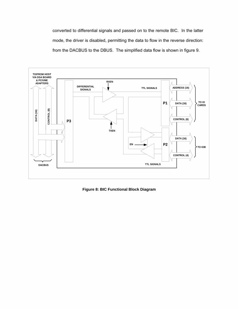
converted to differential signals and passed on to the remote BIC. In the latter

mode, the driver is disabled, permitting the data to flow in the reverse direction:

from the DACBUS to the DBUS. The simplified data flow is shown in figure 9.

P3

P1

P2

CO

NTR

OL

(8)

DA

TA (1

6)

DACBUS

TO/FROM HOSTVIA DSA BOARD

& PCIVMEADAPTERS

ADDRESS (16)

DATA (16)

CONTROL (6)

DATA (16)

CONTROL (4)

DIFFERENTIALSIGNALS TTL SIGNALS

TTL SIGNALS

TO IOCARDS

TO IOB

RXEN

TXEN

EN

Figure 8: BIC Functional Block Diagram

IOB

REMOTE BIC

IO BOARD

CBUS

IO BOARD

RXEN

TXEN

DBUSBIC

REGENERATEDDACBUS

.......

Figure 9: IOB Functional Block Diagram

• DSA board

The DSA board is essentially a bus controller that interfaces two different

buses, VME and DACBUS. The latter is a proprietary bus system developed

by CAE. The DSA is responsible for the data transfer between the host

computer and the MCPI, utilizing the DMA (direct memory address) method.

Its main component is a dual port RAM which is mapped into host

computer’s VME address space. At start up, as part of the initialization, the

host downloads all valid DACBUS addresses to the DSA’s address table

residing in its RAM. During normal operation, the host initiates a transfer

cycle which includes a read and a write operation. During the write

operation, the host sends a block of I/O data (including host memory

address, DACBUS address and word count) to the DSA by writing directly to

its data table (which also resides in the RAM). The DSA then writes the data

out to the MCPI. During a read operation, the host initiates a data request

to the DSA, which then scans the MCPI and stores the data in its data table.

The host then reads the data directly from there. The DSA can operate in

two modes: free run, where it continually cycles through each point in its

address table, writing to or reading from the MCPI, and trigger, where it

scans the MCPI whenever triggered by the hosts. The timing requirement

for a transfer cycle is 50 milliseconds. Any errors encountered during the

transfer cycles (e.g. address time out) are logged into a serial FIFO (first in

first out) memory, where they can be read back to the host for diagnostic

purposes. A simplified block diagram of the DSA is presented in figure 10.

VME BusInterface

Control Registers

Error FIFO

DACBUSInterface

Address Type Status Data

DSA RAM Table

MCPI

Figure 10: DSA Functional Block Diagram

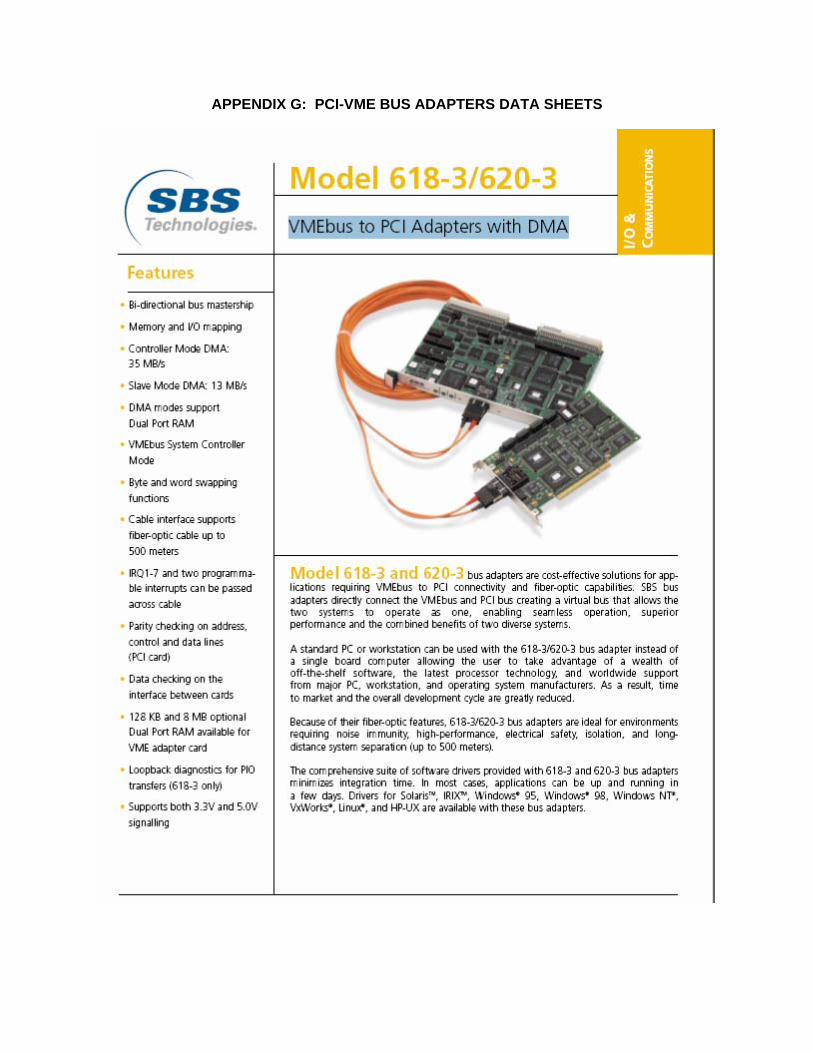
• PCI-VME adapters

The application software running on the Alpha host computer (Unix Tru64

OS) requires some interface to allow it to communicate to the DSA board.

The PCI-VME adapters provide that capability. These bidirectional bus

adapters allow the direct connection between the two bus systems, utilizing

the concept of virtual bus to make them work as one. One of its main

advantages is that it allows the sharing of memory and a special purpose

board between a PCI local bus and VME bus. For the simulator case, this

special purpose board is the DSA board. The PCI-VME adapters are

manufactured by SBS Technologies. A brochure is attached in appendix G.

3.1.2 The new Bus Interface Controller Architecture (eBIC)

As described above, for the old system, the data flow from the host to the function card

goes through several bus systems, namely the PCI, VME, DACBUS, DBUS, and CBUS.

This makes the control and interfacing rather complicated. The eBic, by contrast,

implemented using the ModBus TCP/IP protocol, is far simpler. Its key components are,

as illustrated in figure 11, the microcontroller, the Ethernet controller, the data and

control bi-directional drivers, plus the address drivers.

ETHERNETCONTROLLER

ENC28J60

EPROM32KBYTE

MICROCONTROLLER

dsPIC33FJ256

BIDIRECT-IONAL

DATA &CONTROL

BUSDRIVERS

(22)

ADDRESSBUS

DRIVERS(16)

P1CBUSTO IO

MODULESETHERNET

D00..D15

A00..A15

Figure 11: eBIC Functional Block Diagram

• Microcontroller

The microcontroller is a 16-bit, 40 MIPS digital signal controller, with up to 85

programmable digital I/O pins. The controller operates at 3.3V and also

provides a built-in A/D converter.

• C-Bus drivers and receivers

These drivers provide the necessary electrical interface between the

controller and the function cards. The scanning of the function card is done

via the C-bus.

• Ethernet controller

The Ethernet controller is a stand-alone IEEE 802.3 compatible controller,

with SPI (serial peripheral interface) via which it communicates with

microcontroller.

• EPROM

The memory is basically the storage area for an HTTP server though which

on line diagnostic is provided.

3.2 PREDICTION METHOD SELECTION

The prediction method deemed most suitable for the objective of the project is the MIL-

HDBK-MIL-217F (Notice 2). It was selected because of the following reasons:

• The analysis will be done at the component level.

• Up-to-date, the company (OPG) still accepts reliability evaluations done using

this method from vendors, whenever new electronic designs are to be procured.

• The circuit boards to be evaluated in this project are all used in an OPG

environment. As such it makes sense to employ the same method.

• As mentioned earlier, MIL-217 is still being used by 80% of engineers [13].

• For two of the boards in the old system, the PCI- VME adapters, no schematics

or parts lists are available. Consequently, reliability reports must be obtained

from the vendor. These reports were done using Relex’s MIL-217. Thus, it is

sensible to employ the same method to evaluate other components.

3.3 SOFTWARE AIDS

Calculating the components failure rates of large, complex circuit board is time

consuming. In order to help alleviate the tediousness of the calculation process, it will

be essential that software tools be utilized.

Two software package demos were evaluated. These are the Reliasoft’s Lambda

Predict, and Relex’s suite Architect 2007. Both packages offer a wide variety of

reliability prediction models in their reliability suites, such as Bellcore, HRD5, RDF 2000,

MIL-HDBK-217, etc…While they cost about the same, the Relex suite claims to have a

more extensive component library (400,000 as compared to 240,000 from Reliasoft). In

addition, as shown in appendixes D and E, the prediction reports provided by the vendor

of the PCI-VME adapters (SBS Technologies) are actually prepared using Relex’s

software. As such it is sensible to use the same tool to analyze the rest of the circuit

boards. Consequently, the Relex software was selected as the analysis tool for this

project.

3.4 ANALYSIS PROCESS

The analysis process includes the following steps:

1. Gather needed information, such as bill of materials, schematic (where possible),

and parts data sheets.

2. Calculate required inputs to the prediction software (i.e. operating power)

3. Calculate the failure rates and MTTB of each circuit board using the prediction

software.

4. Summarize the failure rates of the new and existing BICs, and compare the results.

3.5 INPUTS REQUIRED TO THE SOFTWARE

Table 13 shows the inputs required by the Relex software. In addition to these

parameters, the global settings such as temperature and environment (i.e. ground

benign) must be specified at the board level. A snapshot of the prediction data window

for a microprocessor using the MIL-HDBK-217 FN2 (version F, notice 2) is provided in

figure 12.

Prediction Method

Part Type Parameters Required

IC, Microprocessor

Quality Level, Technology, Word Size, Years in Production.

IC, Logic Quality Level, Technology, Number of Gates, Years in Production.

IC, Memory Quality Level, Technology, Type (i.e. Flotox), Number of Bits, Years in Production.

Transistor Quality Level, Power Level (e.g. High or Low). Capacitor Quality Level. Resistor Quality Level, Type (e.g. RN, RL, etc…) Inductor Quality Level, Type (i.e. Fixed or Variable) Diode Quality Level, Type (i.e. rectifier). Crystal Quality Level

Parts Count

Connector Quality Level, Connector Type (e.g. RF Coaxial). IC, Microprocessor

Quality Level, Technology Type (i.e. MOS), Word Size, Pins, Package, Years in Production, Operating Power, Thermal Resistance.

IC, Logic Quality Level, Technology Type (i.e. MOS), Gates, Pins, Package, Years in Production, Operating Power, Thermal Resistance.

IC, Memory Quality Level, Technology Type (i.e. MOS), Type (i.e. Flotox), Bits, Package, Years in Production, Operating Power, Thermal Resistance.

Transistor Quality Level, Operating Voltage and Power, Thermal Resistance, Application, Voltage and Power Ratings .

Capacitor Quality Level, Applied DC Voltage, Voltage Rating, Capacitance, Ambient Temperature.

Parts Stress

Resistor Quality Level, Operating Power, Type (e.g. RN, RL,etc…), Power Rating

Inductor Quality Level, Type (I.e. coil), Hot Spot Temperature. Diode Quality Level, Type (I.e. rectifier), Operating Voltage and

Power, Voltage Rating, Construction Type (i.e. Metallurgically), Thermal Resistance.

Crystal Quality Level, Frequency.

Connector Quality Level, Pairing (i.e. mated), Mating Cycles, Contact Rating, Case Temperature

Table 13: Relex Reliability Prediction Parameters

Figure 12: Typical Relex Prediction Data Window

As mentioned above, the Relex’s software has an extensive components library. Since

information such as technology, maximum ratings (power, voltage and thermal), learning

factor (i.e. years in production) are taken care of by the software, the efforts to find and

provide such information are reduced significantly. Other inputs such as applied voltage

(DC and AC RMS), and operating power are obtained, either from the designer (as the

case of the eBIC), or calculated from the schematics (as the case of the IOB and BIC).

A few samples of such calculations are presented below.

• Power dissipation in ICs:

The following equation from the dsPIC33F (shown as U1 in the eBIC Relex

report) microcontroller data sheet is used to calculate ICs power dissipation:

PD = PINT + PI/O

Where PI/O is the I/O pin power dissipation,

PI/O = ∑ ({VDD – VOH} x IOH) + ∑ (VOL x IOL)

and PINT is the internal power dissipation, calculated as

PINT = VDD (IDD -∑ IOH)

In the above equations, the parameters are defined as follows:

• IOH: output current when the output voltage is high.

• IOL: output current when the output voltage is lo.

• VOH: minimum output voltage when the gate is at logic high level.

• VOL: maximum output voltage when the gate is at logic low level.

• VDD: supply voltage.

• IDD: operating current.

A thorough discussion of these parameters, as applied to digital circuits can be

found in (17).

From the data sheet,

IDD = 74mA (for 40MIPS); VDD = 3.3V; VOH = 2.4V; VOL = 0.4V;

IOH = -3.0mA; IOL = 4mA

Thus, given the number of IOH’s is 9 (8 data lines, plus one clock), and that of

IOL’s is 29 (21 address and control lines, plus 8 data lines), the total power

dissipation would be:

PD = 3.3(74-9*3) + [ 9(3.3-2.4)3.0 + 29*0.4*4] = 0.226W

Alternatively, the typical power dissipation can be approximated using IDD and

VDD, which results in a power dissipation of 244mW (74*3.3). Since the typical

value is larger, for conservative reason, it will be used.

• AC Voltage RMS

In figure 13, a portion of the O/P section of the IOB, presenting a differential data

line, is shown. The differential signal can be approximated as a square wave

having period of T and a duty cycle of 50%, as shown in figure 14.

DUAL LINE DRIVERSN75LS113

D00

D00-1YP

1ZP

Figure 13: IOB Differential Outputs To DACBUS Cable

t

V(t)

Vm

-Vm

T/2 T

Figure 14: Differential Signals Waveform

The RMS voltage can then be calculated as;

Vrms = ∫T

dttVT 0

)(1, where

)(tV = -Vm, for 0 < t T/2, and ≤

)(tV = Vm, for T/2 < t T. ≤

Thus,

Vrms = Vm

Given Vm = 5V, the power dissipated in the resistor can be calculated as:

P = (5)2 / 150 = 167mW.

3.6 ASSUMPTIONS

In performing the reliability prediction of the two I/O architectures, the following

assumptions are made:

• The equipment under consideration is in its normal operating life, hence constant

failure rate is assumed.

• The equipment is operating in a non-mobile, temperature and humidity control

environment. In light of these conditions, the environmental settings are set at

ground benign, 250C.

• The equipment is repairable. Otherwise the definition of MTBF, as presented in

2.2.1 does not apply.

• Where detailed schematics or stress data are not available, the parts count

prediction method will be used. This condition applies to the DSA board.

• In case where even a part list is not available, the vendor reliability report will be

used. This condition applies to the PCI-VME adapters.

3.7 RELIABILITY PREDICTION RESULTS

3.7.1 Prediction Method Summary

As previously mentioned, the prediction method being used to evaluate the individual

hardware components is dictated by the availability of data. If both schematic and BOM

are available, part stress can be used (as power consumption and voltage level can be

calculated); whereas if only BOM is available, part counts is the only option. In the worst

case, where neither schematic nor BOM is available, reliability evaluation must be

obtained from the vendor. The method used for each hardware component is

summarized in table 14.

HW Component Prediction Method Comments

EBIC Board Part Stress Both schematic and BOM are available

BIC Board Part Stress Both schematic and BOM are available

IOB Board Part Stress Both schematic and BOM are available

DSA Board Part Counts Only BOM is available

PCI Adapter Vendor Data Schematic and BOM are not available. Reliability Evaluation provided by vendor

VME Adapter Vendor Data Schematic and BOM are not available. Reliability Evaluation provided by vendor

Table 14: Prediction Method Summary

3.7.2 Reliability Analysis Part Data

While appendices A, B C and F show the final failure rates of the hardware components

of the old and new system, they do not show the specific part data being used. For this

reason, appendix H was provided. It lists all the parameters input into the reliability

software to arrive at the results shown in appendices A, B, C and D. Two snapshots

taken from appendix H will be used to explain where and how the data is used. Figure

15 shows an excerpt from the specific data listing of the EBIC module. In this figure, the

data pertaining to U1 are as follows.

• Type: this field indicates the technology type.

• Quality: commercial grade was used (the eBIC module uses commercial grade

parts, while the existing BIC uses military grade).

• Pi Q: a quality factor of 10 was used as recommended by the handbook, since

the screening process is not known.

• Word: the IC is 16 bit.

• Pin: the 100-pin version was used in the eBic design.

• Package: the flatpack package was used.

• Years: the number of years in production of equal or greater than 2 was used

since the part has been around for a few years.

• Power: the power dissipation as calculated above was used (i.e. 244mW).

• Thermal resistance: a typical thermal resistance of 48.4 for the 100-pin TQFP

(Microchip datasheet) was used.

• Thermal rise: this value is calculated by the software.

Figure 15: eBIC Module Part Stress Data

In figure 16, a snapshot from the specific data listing of the IOB module is shown. As an

example, the parameters used for C2-10 are listed below:

• Quality: these capacitors are military grade.

• Operating DC voltage: from the IOB schematic, these capacitors are operating at

5.0V.

• Their rated voltage is 100V.

• Their voltage ratio is calculated by the software.

• Their capacitance is 10nF.

Figure 16: IOB Module Part Stress Data

The data as explained above are used to populate the fields shown in figure 12. The analysis was run and the failure rates are tabulated in the final prediction reports attached in appendices A, B, C and F. 3.7.3 Results

A summary of the prediction results is shown in table 14. Detailed prediction reports will

be shown in the appendices.

OLD BIC ARCHITECTURE Components Description MTBF (hrs) Failure Rate (/106 hours)

1 PCI bus adapter 202,350 4.941934

2 VME bus adapter 156,394 6.394119

3 DSA board 338,328 2.955715

4 IOB board 294,456 3.396086

5 BIC board 290,332 3.444329

Total 47,321 21.132183

NEW BIC ARCHITECTURE

1 EBIC board 240,454 4.158803

Total 240,454 4.158803

Table 15: Reliability Prediction Results

Note: The combined MTBF of the old system is calculated as 106 / Total failure rate.

3.7.4 Discussion

From table 15, it is quite evident that the new architecture is far more reliable than the

old one. The combined failure rate of the old architecture is 21.132183 (failures per 106

hours), around five times higher than that of the new architecture, 4.158803. The main

factors that contribute to this much higher failure rate are the parts quality, the

components count and the overall system complexity.

3.7.4.1 Parts Quality

Looking at the predictions reports in the appendices, the following can be noticed:

• The highest individual part failure rate is found in the eBIC’s report. The

failure rate of the digital signal processor microcontroller is 1.125343/106

hours. The high rate is mainly due to the complexity of the microcircuit, and

a conservative value of the quality factor used in the calculation of the failure

rate (πQ = 10, as recommended in the handbook for products with unknown

screening level).

• The failure rates of discrete components are low for the BIC and IOB. It is so

because all discrete components used on these boards are of military grade.

The eBIC, on the other hand, uses all commercial grade parts, resulting in

higher failure rates for its discrete parts.

3.7.4.2 Components Count

The most complex board in the old system is the BIC board. It has a components count

of 214. The components count of the new eBIC, in contrast, is only 52. If one were to

add the components of all boards together, the components count of the old system will

be several times higher than that of the new system. From the parts count aspect, a

higher parts count would likely contribute to a higher system failure rate. O’Connor

points out that reducing the number of components and their connections not only

reduces the cost, but also improves the reliability [20]. As such, even though better

quality parts are used in the old design, its combined failure rate is still higher than that

of the new design.

3.7.4.3 System complexity

The existing architecture requires five different circuit boards: the BIC, the DSA board,

the PCI-VME adapters, and the IOB, with five different types of buses, namely the PCI

bus, the VME bus, the DACBUS, the CBUS, and the DBUS. That is not to mention the

two fan-out chassis that are not covered in this analysis, due to the lack of data. This

level of complexity of the existing system makes it rather hard to diagnose, repair and

maintain. In fact, in order to maintain high availability, preventative maintenance has to

be performed on a regular basis. Failed boards are normally replaced instantly with

spares, and then repaired later. As such, at any time, a good spare inventory has to be

maintained. In addition, the system had occasionally failed in such a way that the

provided diagnostic tools fail to pin-point where the problem is. In such situations,

lengthy trouble-shootings are entailed. Finally, due to the complexity of the existing

system, modifications to the I/O system required for different simulator usage are not

easy. For instance, at one point in time, due to the increasing need of simulator usage,

it was required that the simulator be split in half, allowing two training sessions to be run

simultaneously, one on each side (i.e. Unit 2 and Unit 0). To meet that requirement, the

simplest approach was to split the I/O system in half. One half serves Unit 2 control

panels, and the other serves Unit 0. It was found that due to the complexity of the

existing system, splitting the I/O in a certain way affects the quality of the signals, due to

the use of additional hardware (.i.e. switches), causing the I/O system to intermittently

malfunction. In this aspect, it is evident that the existing system is not highly

maintainable. For, the ease to adapt to arising requirement is one important aspect of

maintainability, as defined in section 2.2.5.

The new design, in contrast, consists of only one board, communicating to the simulation

computer via the Ethernet, using MODBUS TCP/IP. The overall architecture is simple

and effective, making it easier to maintain, and hence more reliable. In addition, since it

is implemented using the well-established MODBUS TCP/IP protocol, a widely used

protocol in the industry, it would be easy to modify it to meet future requirement, should

such a need arise. Even though the eBIC is still in its design stage, it has already been

foreseen that the task of splitting up the simulator as described above, would be straight

forward, as no additional hardware is required to achieve that goal. Further, in the

existing system, the use of the intermediate circuit boards operating on different types of

buses requires different drivers to be written (for instance, the DSA board), or acquired

(i.e. the PCI-VME adapters). Such an issue will not arise with the eBIC, as it utilizes the

standard TCP/IP protocol. Writing an application to handle the I/O communication is, in

general, simpler using TCP/IP, as compared to other bus architectures. Finally, the

simulation software is currently running on Tru64 Unix, a soon-to-be obsolete OS. It is

inevitable that the simulation software will, sooner or later, have to be migrated to

another OS. Be it Windows or be it Linux, the task of converting the I/O application from

Unix to other operating systems will not be an issue, as the implementation of the

TCP/IP protocol would be greatly similar between different platforms.

3.7.5 Recommendation

As described in section 3.1.1, the timing requirement for a complete I/O transfer cycle is

50ms. This is an important requirement due to the real-time nature of the simulation

software application. As of the writing of this report, a program has been written to test

the communication of the eBIC to the Alpha computer, and to preliminarily evaluate the

performance of the new design. While the board works well, it was observed that

timeouts do occur occasionally. Although this is normal for a network application, and

the program can be written to minimize the effect of the timeouts (i.e. retry), it would be

desirable to not have the timeouts at all. The eBIC is currently built around a 16-bit DSP

microcontroller. It is expected that the use of a 32-bit DSP microcontroller will

significantly boost the performance of the board, thus eliminating the timeout issue.

Further, commercial grade parts are used in the eBIC design; it is expected that using

military grade would yield higher reliability.

CHAPTER 4: CONCLUSION

As summarized in the last section, the new eBIC design possesses many outstanding

features. It is designed with the capability to adapt to new requirements, be it the

expansion of the hardware, or be it the migration of the software application. The eBIC

eliminates all intermediate hardware required by the old system, such as the PCI-VME,

the DSA, and the IOB circuit boards. As such, it greatly simplifies the hardware

architecture. The end results are the reduced cost and the higher maintainability. At the

beginning, it is expected that due to its many advantages over the old system, the eBIC

will be more reliable and robust. The results of the reliability evaluation have proved just

that: the predicted failure rate of the new system is five times lower than the failure rate

of the existing system; its predicted MTBF of approximately 27 years looks rather

promising, and would even stand out better, considering the (overly) pessimistic nature

of the MIL-217. As this is a new design, the incorporation of the reliability evaluation into

the design cycle is useful, especially in raising the level of confidence in the new design.

REFERENCES

1. The Institute of Electrical and Electronics Engineers, “IEEE Standard Computer

Dictionary: A Compilation of IEEE Standard Computer Glossaries”, New York, 1990.

2. “MIL-HDBK-338B Electronic Design Handbook”, Department of Defense, USA,

October 1, 1998.

3. http://parts.jpl.nasa.gov

4. Torelli, Wendy and Avelar, Victor, “Mean Time Between Failure: Explanation and

Standards”, APC, Kingston, 2004.

5. Scheaffer, Richard and McClave, T. James, “Probability for Statistics for Engineer”s,

Duxbury Press, USA, 1995.

6. Dhillon, B.S, Reliability, “Quality and Safety for Engineers”, CRC Press, USA, 2004.

7. MIL-HDBK-217F Notice 2, “Reliability Prediction of Electronic Equipment”,

Department of Defense, USA , Feb. 1995.

8. Ward, Tony, Ward, A E and Angus, James, “Electronic Product Design”, CRC Press,

USA, 1996.

9. http://www.amsaa.army.mil

10. http://www.calce.umd.edu/

11. The FIDES group, “FIDES Guide 2004 issue AReliability Methodologyfor Electronic

Systems”, http://fides-reliability.org, 2007.

12. Marin, J. J, Pollard, R. W, “Experience report on the FIDES reliability prediction

method”, Annual Reliability and Maintainability Symposium, IEEE, 2005.

13. White, Mark, Bernstein, Joseph, “Microelectronics Reliability: Physics-of-Failure

Based Modeling and Lifetime Evaluation”, Jet Propulsion Laboratory, California,

2008.

14. Vintr, M., “Reliability Assessment for Components of Complex Mechanisms and

Machines”, Brno University of Technology, Czech Republic, 2007.

15. Goel, Anuj, and Graves, J. Robert, “Electronic System Reliability: Collating Prediction

Models”, IEEE Transactions on Device and Materials Reliability, Vol. 6, No. 2, June

2006.

16. www.actel.com

17. Faraci, Vito Jr., “Hazadous Events”, Reliability Analysis Centre, BAE Systems, US,

2004.

18. Yun, Young Won, “Reliability Evaluation on Digital Control Module Used In ABB-CE

Nuclear Power Plan in Korea”, Korea Institution of Nuclear Safety, Taejeon, 2000.

19. Torelli, Wendy and Avelar, Victor, “Performing Effective MTBF Comparisons for Data

Center Infrastructure”, APC, Kingston, 2004.

20. O’Connor, Patrick D.T, “Practical Reliability Engineering”,” 4th edition, Wiley, 2002.

21. Bali, S. P, “2000 Solved Problems in Digital Electronics”, Tata McGraw-Hiil, 2005.

22. www.weibull.com/hotwire/issue22/hottopics22.htm

23. http://www.rfhic.com/data/qnr/Mixer/MU0941.pdf

24. Bowles, B. Jones, “A Survey of Reliability-Prediction Procedures For Microelectronic

Devices”, IEEE Transaction On Reliability, Vol. 41, 1992.

APPENDIX A: BIC BOARD RELIABILITY PREDICTION REPORT

APPENDIX B: IOB BOARD RELIABILITY PREDICTION REPORT

APPENDIX C: DSA BOARD RELIABILITY PREDICTION REPORT

APPENDIX D: PCI ADAPTER VENDOR RELIABILITY PREDICTION REPORT

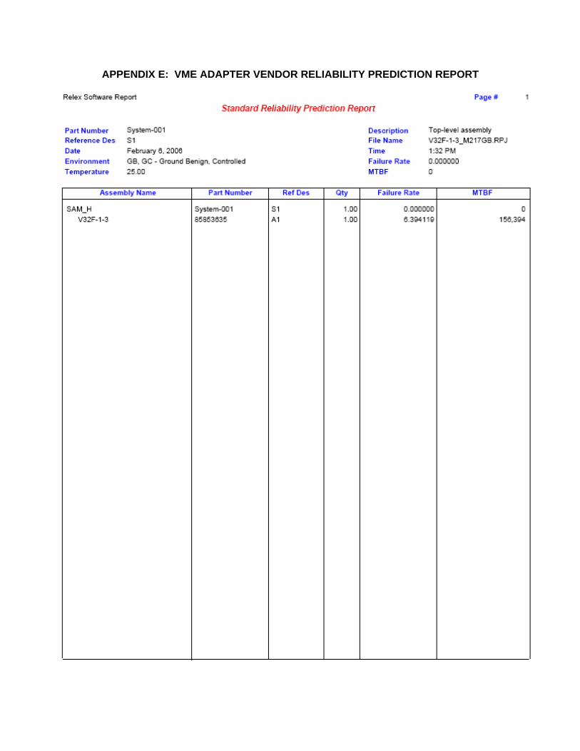
APPENDIX E: VME ADAPTER VENDOR RELIABILITY PREDICTION REPORT

APPENDIX F: eBIC ADAPTER RELIABILITY PREDICTION REPORT

APPENDIX G: PCI-VME BUS ADAPTERS DATA SHEETS

APPENDIX H: DETAILED SPECIFIC PART DATA