C. Ebeling, Intro to Reliability & Maintainability Engineering, 2nd ed. Waveland Press, Inc. Copyright © 2010

Chapter 13Reliability Testing

13.1 Product Testing 13.2 Reliability Life Testing13.3 Test Time Calculations13.4 Burn-in & screen testing13.6 Accelerated life testing

Test Design

• Test objective• e.g. reliability demonstration, reliability improvement,

screening

• Type of test• e.g. sequential, accelerated

• Operating & environmental conditions• Number of units to be tested (sample size)• Duration of test

• failure terminated vs time terminated• Definition of a failure

Chapter 13 2

Cumulative Time on Test - CFR

Chapter 13 3

n = nbr on testr = nbr failuresk = nbr multiply censorsti = failure timeti

+ = censor timet* = test time (Type I)tr = test time (Type II)

MTTF = T / r

( )

( )

( )

( )

1

*1

1

*1

1

*

Complete: ;

TypeI:

TypeII:

TypeI multiply:

TypeII multiply:

TypeI replacement:TypeII replacement:

n

ii

n

ii

n

i ri

n

ii

n

i ri

r

t r n

t n r t

t n r t

t n r k t

t n r k t

ntnt

=

=

=

+

=

+

=

=

+ −

+ −

+ − −

+ − −

∑

∑

∑

∑

∑

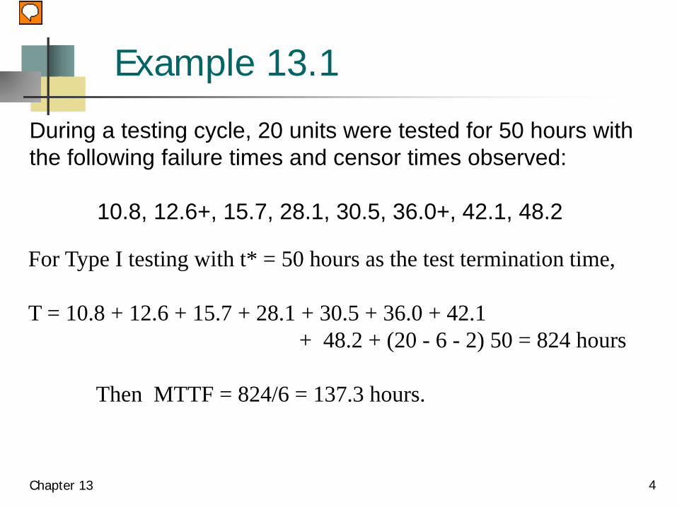
Example 13.1

Chapter 13 4

During a testing cycle, 20 units were tested for 50 hours with the following failure times and censor times observed:

10.8, 12.6+, 15.7, 28.1, 30.5, 36.0+, 42.1, 48.2

For Type I testing with t* = 50 hours as the test termination time,

T = 10.8 + 12.6 + 15.7 + 28.1 + 30.5 + 36.0 + 42.1 + 48.2 + (20 - 6 - 2) 50 = 824 hours

Then MTTF = 824/6 = 137.3 hours.

Example 13.2

Chapter 13 5

Ten units were placed on test with a failed unit immediately replaced. The test was terminated after the 8th failure which occurred at 20 hours.

This is type II testing with replacement. Therefore

T = (10) (20) = 200 hours

MTTF = 200/8 = 25 hours

Length of Test - Type II Testing - CFR

Chapter 13 6

with replacement:

λ = failure rate of single unit

n λ = system failure rate with n units operating

1/(n λ) = MTTF/n = system MTTF

E(test time) = r x MTTF / n

Length of Test - Type II Testing - CFR

Chapter 13 7

E test time MTTF x TTF = MTTF 1n

+ 1n -1

+...+ 1n - r + 1r n( ) ,= L

NMOQP

without replacement: generate r failures:

With n units on test: system MTTF = MTTF/n With n-1 units on test: system MTTF = MTTF/(n-1)With n-2 units on test: system MTTF = MTTF/(n-2)

With n-r+1 units on test: system MTTF = MTTF/(n-r+1)

TTFr,n

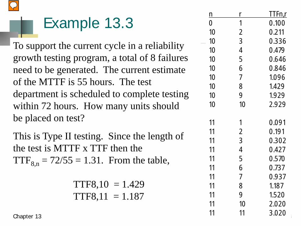
Example 13.3

Chapter 13 8

To support the current cycle in a reliability growth testing program, a total of 8 failures need to be generated. The current estimate of the MTTF is 55 hours. The test department is scheduled to complete testing within 72 hours. How many units should be placed on test?

This is Type II testing. Since the length of the test is MTTF x TTF then the TTF8,n = 72/55 = 1.31. From the table,

TTF8,10 = 1.429TTF8,11 = 1.187

n r TTFn,r0 1 0.100 10 2 0.211 10 3 0.336 10 4 0.479 10 5 0.646 10 6 0.846 10 7 1.096 10 8 1.429 10 9 1.929 10 10 2.929

11 1 0.091 11 2 0.191 11 3 0.302 11 4 0.427 11 5 0.570 11 6 0.737 11 7 0.937 11 8 1.187 11 9 1.520 11 10 2.020 11 11 3.020

Example 13.4

Chapter 13 9

For the problem in Example 13.3, the test department is told they must complete the testing within 48 hours. How many failures would they expect to generate?

E(r) = 11(1- e ) = 6.4 units- 4855

Burn-in Testing

Goal is to increase the mean residual life

Eliminate “early” customer failures by generating test

hours in the factory

There must be a dominate DFR failure mode

Primary question is how long to test?

Specification model

cost model

Chapter 13 10

Burn-in Testing Specification Model

Chapter 13 11

Given a reliability goal of R0 where R(t0 ) < R0 and R(t) has a DFR, then a burn-in period, T, is desired such that R(t0 | T) = R0.

For the Weibull distribution

R t T e

e

R

t T

T( | )0 0

0

= =−

+FHGIKJ

−FHGIKJ

θ

β

θ

β

e R et T T

−+FHGIKJ −FHG

IKJ− =

0

0 0θ

β

θ

β

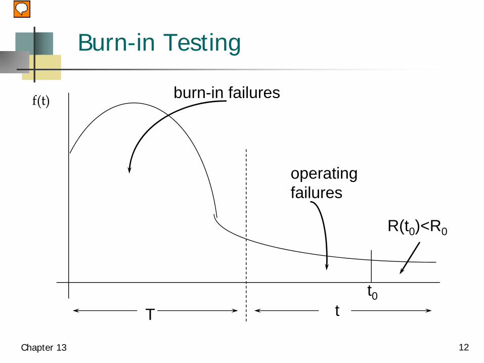
Burn-in Testing

Chapter 13 12

burn-in failures

operatingfailures

T tt0

R(t0)<R0

f(t)

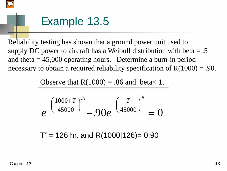
Example 13.5

Chapter 13 13

Reliability testing has shown that a ground power unit used to supply DC power to aircraft has a Weibull distribution with beta = .5 and theta = 45,000 operating hours. Determine a burn-in period necessary to obtain a required reliability specification of R(1000) = .90.

Observe that R(1000) = .86 and beta< 1.

e eT T

−+F

HGIKJ −FHG

IKJ− =

100045000

5

4500090 05.

..

T* = 126 hr. and R(1000|126)= 0.90

Burn-in Testing - Cost Model

Chapter 13 14

Cb = cost per unit time for burn-in testingCf = cost per failure during burn-inCo = cost per failure when operationalT = length of burn-in testingt = operational life of the units

E[C(T)] = Cb T + Cf [ 1 - R(T)] + Co [ R(T) - R(t+T) ]

for the Weibull:

[ ( )] 1T T T t

b f oE C T C T C e C e eβ β β

θ θ θ+⎛ ⎞ ⎛ ⎞ ⎛ ⎞− − −⎜ ⎟ ⎜ ⎟ ⎜ ⎟

⎝ ⎠ ⎝ ⎠ ⎝ ⎠⎡ ⎤ ⎡ ⎤⎢ ⎥ ⎢ ⎥= + − + −⎢ ⎥ ⎢ ⎥⎣ ⎦ ⎣ ⎦

Example 13.6

Chapter 13 15

The replacement cost on a new product if it fails during its operational life of 10 years (3650 days) is $6200. It will cost the company $70 a day per unit tested to operate a burn-in program and any failures during burn-in will cost $500. Reliability testing has established the life distribution of the product to be Weibull with beta = .35, and theta = 3500 days. What is the minimum cost time period for the burn-in?

3650.35 .35 .353500 3500 3500[ ( )] 70 500[1 ] 6200 [ ]

T T T

E C T T e e e+⎛ ⎞ ⎛ ⎞ ⎛ ⎞− − −⎜ ⎟ ⎜ ⎟ ⎜ ⎟

⎝ ⎠ ⎝ ⎠ ⎝ ⎠= + − + −

T* = 1.9 days with E[C(T)] = $ 3690

Example 13.6

Chapter 13 16

362036403660368037003720374037603780380038203840

Expected Cost

Burn-in Time (days)

E[C(T)]=$ 3690

T = 0, E[C(T)] = $3952

E[C(T)] = $3704

Accelerated Life Testing

• Increase the number of units on test (compressed time)

• Accelerate the number of cycles per unit of time

• Increase the stresses that generate failures (accelerated stress testing)

Chapter 13 17

Problem: test time < expected lifetimesSolution:

Increase Number of Units on Test

Chapter 13 18

fTTFTTFr n

n r

r r,

,

,

=For CFR: without replacement

fr,n = r/n with replacement

fr,n is the factor reduction in expected test time100(1-fr,n) is the percent savings in expected test time

then

Increase Number of Units on Test

Chapter 13 19

fTTFTTFr n

n r

r r,

,

,

/

=FHGIKJ

1 βfor Weibull: without replacement

f rnr n,

/

= FHGIKJ

1 β

with replacement

fr,n is the factor reduction in expected test time100(1-fr,n) is the percent savings in expected test time

then

Example 13.10

Chapter 13 20

Given n = 15 and r = 8:

without replacement with replacement

CFR model: f8,15 = TTF8,15 / TTF8,8 f8,15 = 8/15 = .533 = .725/2.718 = .2667

Weibull f8,15 = (.725/2.718)1/2 f8,15 = (8/15)1/2 = .730(Beta = 2) = .516

replacing vs not replacing failed units: ( ),

8 .735615 0.725r n

rnTTF

= =

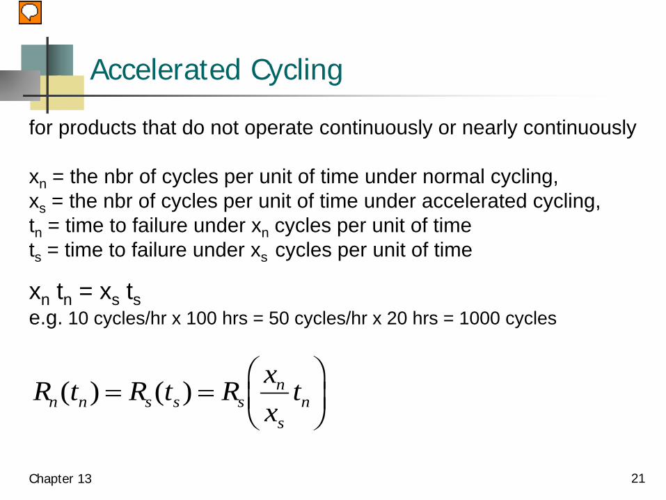
Accelerated Cycling

Chapter 13 21

for products that do not operate continuously or nearly continuously

xn = the nbr of cycles per unit of time under normal cycling,xs = the nbr of cycles per unit of time under accelerated cycling,tn = time to failure under xn cycles per unit of timets = time to failure under xs cycles per unit of time

xn tn = xs tse.g. 10 cycles/hr x 100 hrs = 50 cycles/hr x 20 hrs = 1000 cycles

R t R t R xx

tn n s s sn

sn( ) ( )= =

FHGIKJ

An Observation

Chapter 13 22

[ ] [ ]

[ ] [ ]2 2

2

n n n ns n s n n n

s s s s

n n ns n n n

s s s

x x x xT T and E T E T E Tx x x x

x x xVar T Var T Var Tx x x

μ

σ

⎡ ⎤= = = =⎢ ⎥

⎣ ⎦

⎡ ⎤ ⎛ ⎞ ⎛ ⎞= = =⎜ ⎟ ⎜ ⎟⎢ ⎥

⎣ ⎦ ⎝ ⎠ ⎝ ⎠

Let Ts = a random variable, the time to failure under accelerated cyclingTn = a random variable, the time to failure under normal cycling

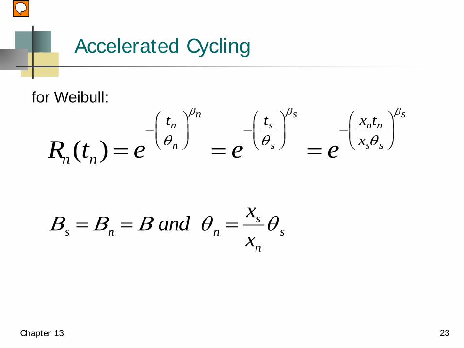
Accelerated Cycling

Chapter 13 23

for Weibull:

R t e e en n

t t x tx

n

n

ns

s

sn n

s s

s

( ) = = =−FHGIKJ −

FHGIKJ −

FHGIKJθ θ θ

β β β

Β Β Βs n ns

nsand x

x= = =θ θ

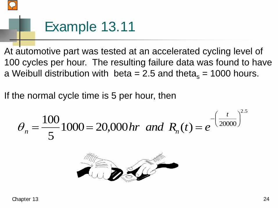
Example 13.11

Chapter 13 24

At automotive part was tested at an accelerated cycling level of 100 cycles per hour. The resulting failure data was found to have a Weibull distribution with beta = 2.5 and thetas = 1000 hours.

If the normal cycle time is 5 per hour, then

θn n

t

hr and R t e= = =−FHG

IKJ100

51000 20 000 20000

2 5

, ( ).

Accelerated Cycling and the Normal Distribution

Chapter 13 25

( ) 1 1

1 1

therefore: and

n n s sn n

n s

n sn s n s

s n

sss

n

s sn s n s

n n

t tR t

x xt tx x

xx

x xx x

μ μσ σ

μ μ

σ σ

μ μ σ σ

⎛ ⎞ ⎛ ⎞− −= −Φ = −Φ⎜ ⎟ ⎜ ⎟

⎝ ⎠ ⎝ ⎠⎛ ⎞ ⎛ ⎞− −⎜ ⎟ ⎜ ⎟⎜ ⎟ ⎜ ⎟= −Φ = −Φ⎜ ⎟ ⎜ ⎟⎜ ⎟ ⎜ ⎟⎝ ⎠ ⎝ ⎠

= =

Accelerated Cycling and the LogNormal Distribution

Chapter 13 26

,

,,

, ,

1 1( ) 1 ln 1 ln,

1 11 ln 1 ln

therefore: and

n sn n

n med n s med

nn

s n

ss med s smed s

n

smed n med s n s

n

t tR ts t s t s

x tx t

xs t s tx

xt t s sx

⎛ ⎞ ⎛ ⎞= −Φ = −Φ⎜ ⎟ ⎜ ⎟⎜ ⎟ ⎝ ⎠⎝ ⎠

⎛ ⎞ ⎛ ⎞⎜ ⎟ ⎜ ⎟⎜ ⎟ ⎜ ⎟= −Φ = −Φ⎜ ⎟ ⎜ ⎟⎜ ⎟ ⎜ ⎟⎝ ⎠ ⎝ ⎠

= =

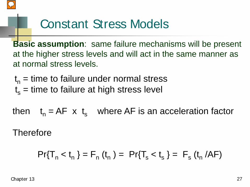
Constant Stress Models

Chapter 13 27

Basic assumption: same failure mechanisms will be presentat the higher stress levels and will act in the same manner asat normal stress levels.

tn = time to failure under normal stressts = time to failure at high stress level

then tn = AF x ts where AF is an acceleration factor

Therefore

Pr{Tn < tn } = Fn (tn ) = Pr{Ts < ts } = Fs (tn /AF)

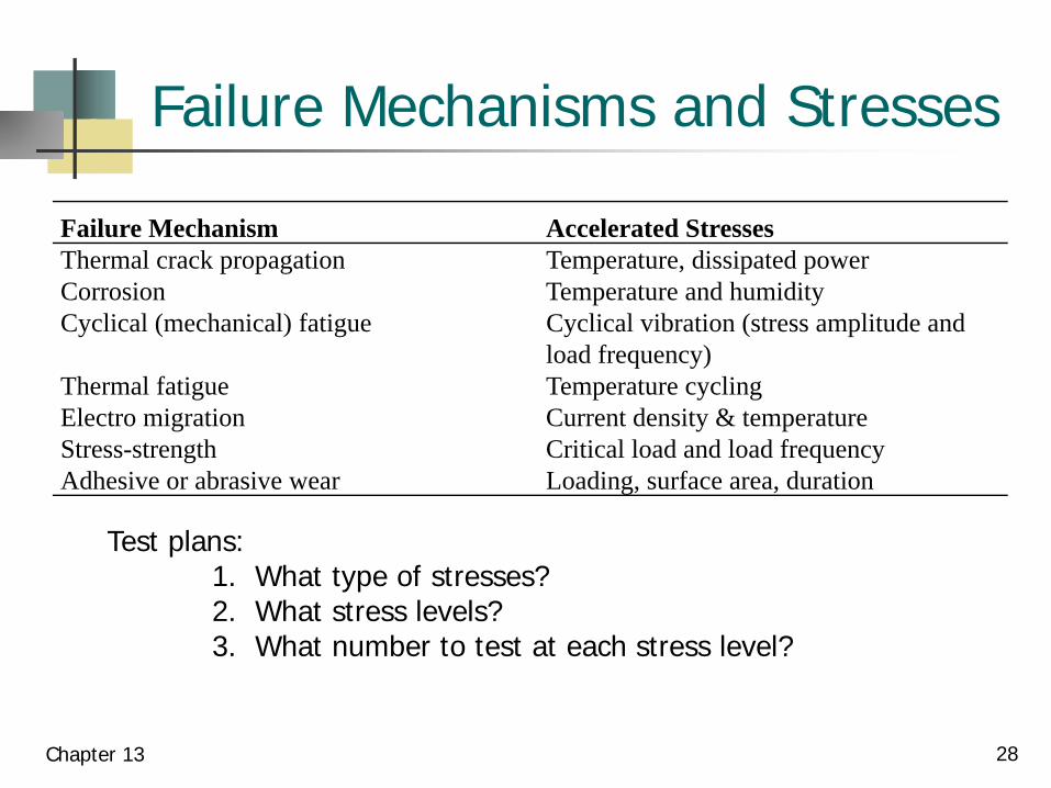
Failure Mechanisms and Stresses

Chapter 13 28

Test plans:1. What type of stresses?2. What stress levels?3. What number to test at each stress level?

Failure Mechanism Accelerated StressesThermal crack propagation Temperature, dissipated powerCorrosion Temperature and humidityCyclical (mechanical) fatigue Cyclical vibration (stress amplitude and

load frequency)Thermal fatigue Temperature cyclingElectro migrationStress-strengthAdhesive or abrasive wear

Current density & temperatureCritical load and load frequencyLoading, surface area, duration

Example 13.12

Chapter 13 29

For the CFR model, a component is tested at 120°C and found to have an MTTF = 500 hours. Normal use is at 25°C. Assuming AF = 15, determine the components MTTF and reliability function at normal stress levels.

n s- t

AFF (t) = Ft

AF = 1-e s

FHGIKJ

FHGIKJλ = 1-e- t

500x15

R(t) = e- t7500 and MTTF = 7500 hr.

Weibull Case

Chapter 13 30

s- t

F (t) = 1-es

s

β

θFHGIKJ

n- t

AFF (t) = 1-es

s

β

θFHGIKJ

n s n s = AFx = .θ θ β βand

estimate AF by:^

^n

s

AF = θθ

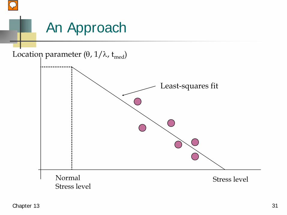
An Approach

Chapter 13 31

Stress level

Location parameter (θ, 1/λ, tmed)

NormalStress level

Least-squares fit

Example 13.15

Accelerated life testing for fracture stress failures at high temperature was conducted on 40 units at four different accelerated stress levels with the following results in hours:

Chapter 13 32

Βθ

stress level* 7 8 9 10sample time to fail time to fail time to fail time to fail

1.0 4355 1677 784 10672.0 4951 4707 1813 6813.0 7503 2407 2240 13394.0 1475 1367 2731 11515.0 4703 5709 1533 14366.0 5002 2976 1639 5077.0 4091 2343 1979 11748.0 2514 2879 1612 6559.0 4775 3551 1233 1156

10.0 1898 2804 1705 773

*stress levels are measured in psi

Example 13.15

Chapter 13 33

stress level 7 8 9 10

β 2.7 2.5 3.2 3.1

θ 4647 3445 1938 1117

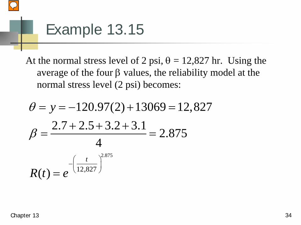
Example 13.15

At the normal stress level of 2 psi, θ = 12,827 hr. Using the average of the four β values, the reliability model at the normal stress level (2 psi) becomes:

Chapter 13 34

2.875

12,827

120.97(2) 13069 12,8272.7 2.5 3.2 3.1 2.875

4

( )t

y

R t e

θ

β

⎛ ⎞−⎜ ⎟⎝ ⎠

= = − + =+ + +

= =

=

Nonlinear stress effects

Assume , m ≠ 1.

both the scale and shape parameters change

Chapter 13 35

mn st kt=

( )( )

ss/n

1/n

n nn s

1 exp 1 exp 1 expm

mn n

ms

t ttF tk k

βββ

θ θ θ

⎡ ⎤⎡ ⎤⎡ ⎤ ⎛ ⎞⎛ ⎞⎛ ⎞ ⎢ ⎥⎢ ⎥⎢ ⎥= − − = − − = − −⎜ ⎟⎜ ⎟⎜ ⎟ ⎜ ⎟⎢ ⎥⋅ ⋅⎢ ⎥⎢ ⎥⎝ ⎠ ⎝ ⎠ ⎝ ⎠⎣ ⎦ ⎣ ⎦ ⎣ ⎦

Arrhenius Modelused when increased temperature is the applied stress

Chapter 13 36

r = Ae- BT

where r is the reaction or process rate, A and B are constants, and T is temperature measured in degrees Kelvin

AF = AeAe

= e- BT

- BT

B ( 1T

- 1T

)2

1

1 2

1

2

ln

1 2

AFB = where AF1 1( - )T T

θθ

=

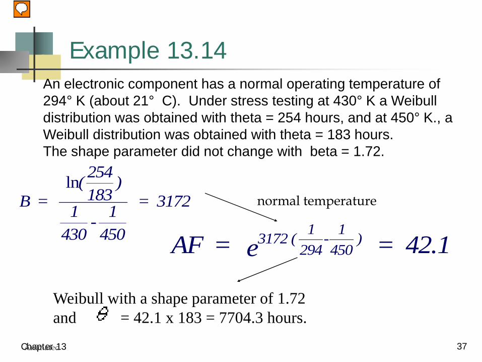
Example 13.14

Chapter 13 37

An electronic component has a normal operating temperature of 294° K (about 21° C). Under stress testing at 430° K a Weibull distribution was obtained with theta = 254 hours, and at 450° K., a Weibull distribution was obtained with theta = 183 hours. The shape parameter did not change with beta = 1.72.

B = ( 254183

)

1430

- 1450

= 3172ln

AF = e = 42.13172 ( 1294

- 1450

)

Weibull with a shape parameter of 1.72 and = 42.1 x 183 = 7704.3 hours.

Animated

normal temperature

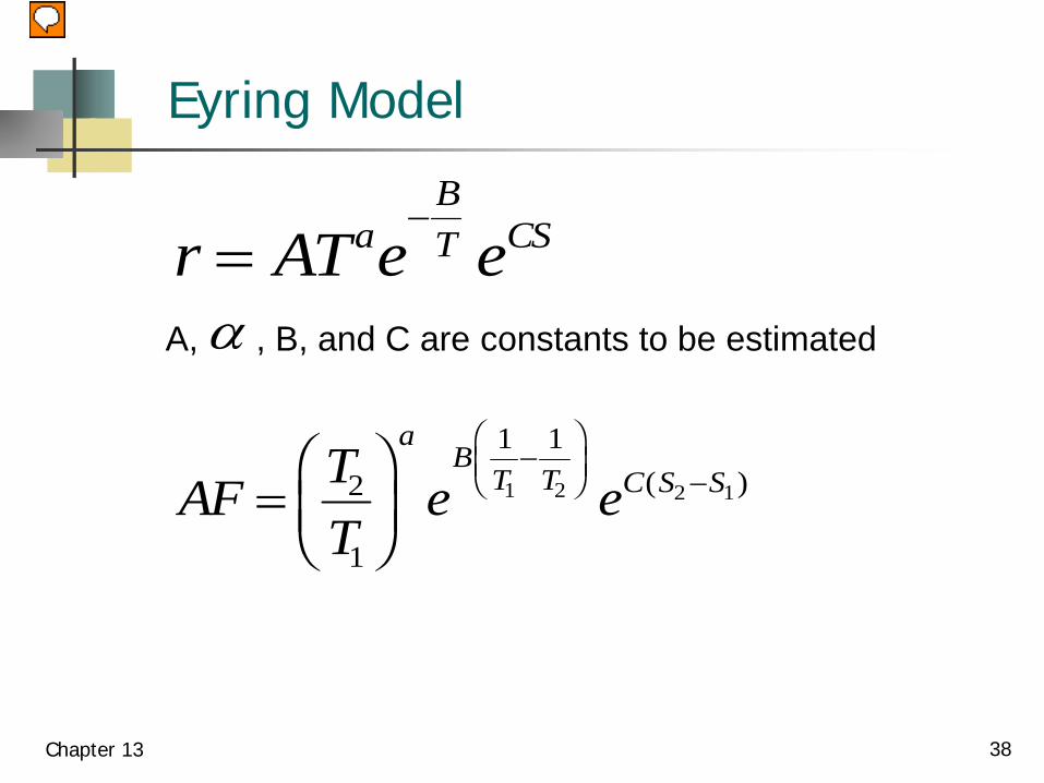
Eyring Model

Chapter 13 38

r AT e eaBT CS=

−

AF TT

e ea

BT T C S S=

FHGIKJ

−FHGIKJ −2

1

1 1

1 2 2 1( )

A, , B, and C are constants to be estimatedα

Degradation Models

Chapter 13 39

y = a - b t , where y is the performance measure, a and b are constants to be determined experimentally, and t is the amount of time the product is exposed at a constant stress level

ta y

bff=

−time to failure, tf :

where yf is the performance level at which a failure occurs

Example 13.15

Chapter 13 40

CPR kw tAt

=( )

ρt = exposure time in hours,w(t) = weight loss due to corrosion after t hours exposure in mg

= density of the material in grams per cubic centimeterA = exposed surface area in square centimetersk = 87.6, a constant which converts CPR to millimeters per year

If lf is the allowable loss in millimeters after which the material is no longer structurally sound, then the time to failure is projected to be

tf = lf / CPR

Example 13.16

Chapter 13 41

p e rt= −where p = potency of the drugr = rate of chemical reactiont = drug exposure time

then t = - ln p / r

r Ae then t pAe

BT

B T= =−−

−

ln/

Cumulative Damage Models

Chapter 13 42

tL

i

ii

n

=∑ =

1

1

Minor’s rule:

ti = the amount of time at stress level iLi = the expected lifetime at stress level i

tL

tL

or t L LL

t1

1

2

22 2

2

111+ = = −

Cumulative Damage Models

Chapter 13 43

normal stress timeL1

L2failure line

t2

t1

high stress time

1. test to failure

2. test to t1 then to failure t2

L ttL

11

2

2

1=

−

3. solve

The End of Chapter 13

Chapter 13 44

I have found this discussion

to be quite stress full

I feel I have degraded in an

accelerated way!