Journal of Applied Mathematics and Physics, 2014, 2, 1242-1256 Published Online December 2014 in SciRes. http://www.scirp.org/journal/jamp http://dx.doi.org/10.4236/jamp.2014.213145

How to cite this paper: Yusuf, I., et al. (2014) Reliability Modelling and Analysis of Redundant Systems Connected to Sup-porting External Device for Operation Attended by a Repairman and Repairable Service Station. Journal of Applied Mathe-matics and Physics, 2, 1242-1256. http://dx.doi.org/10.4236/jamp.2014.213145

Reliability Modelling and Analysis of Redundant Systems Connected to Supporting External Device for Operation Attended by a Repairman and Repairable Service Station Ibrahim Yusuf1, Rabia Salihu Said2, Fatima Salman Koki2, Mansur Babagana3 1Department of Mathematical Sciences, Bayero University, Kano, Nigeria 2Department of Physics, Bayero University, Kano, Nigeria 3Department of Computer Science and Information Technology, Bayero University, Kano, Nigeria Email: iyusuf.mth@buk.edu.ng, rssaidu.phy@buk.edu.ng, FatimaSK2775@gmail.com, mbabagana.cs@buk.edu.ng Received 5 October 2014; revised 1 November 2014; accepted 24 November 2014

Copyright © 2014 by authors and Scientific Research Publishing Inc. This work is licensed under the Creative Commons Attribution International License (CC BY). http://creativecommons.org/licenses/by/4.0/

Abstract In this paper, probabilistic models for three redundant configurations have been developed to analyze and compare some reliability characteristics. Each system is connected to a repairable supporting external device for operation. Repairable service station is provided for immediate repair of failed unit. Explicit expressions for mean time to system failure and steady-state avail-ability for the three configurations are developed. Furthermore, we compare the three configura-tions based on their reliability characteristics and found that configuration II is more reliable and efficient than the remaining configurations.

Keywords Availability, Supporting Device, Service Station, Redundancy

1. Introduction High system reliability and availability play a vital role towards industrial growth as the profit is directly de-pendent on production volume which depends upon system performance. Thus the reliability and availability of a system may be enhanced by proper design, optimization at the design stage and by maintaining the same dur-

I. Yusuf et al.

1243

ing its service life. Because of their prevalence in power plants, manufacturing systems, and industrial systems, many researchers have studied reliability and availability problem of different systems (see, for instance, Ref [1]-[8] and the references therein). In real-life situations we often encounter cases where the systems that cannot work without the help of external supporting devices connect to such systems. These external supporting devices are systems themselves that are bound to fail. Where such systems exist, a repairable service station is provided for the immediate repair of failed unit. Such systems are found in power plants, manufacturing systems, and in-dustrial systems. Ref [9] [10] performed comparative analysis of some reliability characteristics between redun-dant systems requiring supporting units for their operation.

The problem considered in this paper is different from the work of Ref [9] [10]. The objectives of the present paper are three. The first is to develop the explicit expressions for the mean time to system failure (MTSF) and steady- state availability. The second objective is to perform a parametric investigation of various system parameters on mean time to system failure (MTSF) and steady-state availability and capture their impact on the mean time to sys- tem failure (MTSF) and steady-state availability. The third objective is to perform comparative analysis between the three configurations based on assumed numerical values in order to determine the optimal configuration.

2. Description of the Systems We consider three redundant systems connected to an external supporting device for their operation as follows. The first system is a 2-out-of-3 system connected to a supporting device and has a repairable service station. The second is also a 2-out-of-3 system connected to supporting device and has two standby repairable service sta-tions. The third system is a 3-out-of-4 system connected to a supporting device and has a repairable service sta-tion. We assume that switching is perfect and instantaneous. We also assume that two units cannot fail simulta-neously. Whenever a unit fails with failure rate 1β , it is immediately sent to a service station for repair with service rate 1α . However, on the course of repairing failed unit, the service is bound to fail with failure rate of

2β and service rate of 2α and failed unit must wait whenever the service station is under repair for first and third system, while the standby service will continue repairing failed unit for the second system. The supporting device is a system that is prone to failure. Whenever the supporting device failed with rate 3β it is attended by a repairman, the system stop working and must wait until the supporting device is repaired with rate 3α .

3. Mean Time to System Failure Models Formulation 3.1. MTSF Formulation for Configuration I For configuration I, we define ( )iP t to be the probability that the system at time 0t ≥ is in state iS . Also let ( )P t be the probability row vector at time t , we have the following initial condition:

( ) ( ) ( ) ( ) ( ) ( ) ( ) ( ) ( ) [ ]0 1 2 3 4 5 6 70 0 , 0 , 0 , 0 , 0 , 0 , 0 , 0 1,0,0,0,0,0,0,0P P P P P P P P P= =

We obtain the following differential equations: ( ) ( ) ( ) ( ) ( )( ) ( ) ( ) ( ) ( ) ( )( ) ( ) ( )( ) ( ) ( ) ( ) ( )( ) ( ) ( ) ( ) ( )( ) ( ) ( ) ( ) ( )( ) ( )

01 2 0 1 1 2 2

31

1 1 1 0 3 3 1 4 2 51

22 2 2 0

33 1 2 3 3 1 2 7

41 3 4 1 1 3 6

52 3 5 2 1 3 7

63 6

dd

dd

dd

dd

dd

dd

dd

kk

P tP t P t P t

tP t

P t P t P t P t P tt

P tP t P t

tP t

P t P t P tt

P tP t P t P t

tP t

P t P t P tt

P tP t

t

β β α α

α β β α α α

α β

α β β β α

α β β α

α β β α

α β

=

= − + + +

= − + + + + +

= − +

= − + + + +

= − + + +

= − + + +

= − +

∑

( ) ( )( ) ( ) ( ) ( ) ( )

1 3 3 4

72 3 7 2 3 3 5

dd

P t P tP t

P t P t P tt

β

α α β β

+

= − + + +

(1)

I. Yusuf et al.

1244

This can be written in the matrix form as

1P T P= (2) where

( )

( )( )

( )

( )

1 2 1 23

1 1 3 1 21

2 2

3 3 1 2 21

1 1 3 3

2 2 3 3

1 3 3

2 3 2 3

0 0 0 0 0

0 0 0

0 0 0 0 0 00 0 0 0 00 0 0 0 00 0 0 0 00 0 0 0 00 0 0 0 0

kk

T

β β α α

β α β α α α

β αβ α β β αβ α β αβ α β α

β β αβ β α α

=

− + − + − − + += − + − +

− − +

∑

It is difficult to evaluate the transient solutions, the procedure to develop the explicit expression for 1MTSF is to delete the rows and column of absorbing states of matrix 1T and take the transpose to produce a new ma-trix, say 1M . Following Ref [11] [12], the expected time to reach an absorbing state is obtained from

( ) ( ) ( )( )1 01 10 absorbing

0

10 1

1P P

NE T MTSF P Q

D−

→

= = − =

(3)

where ( )

( )

1 2 13

1 1 1 31

3 3 1 2

0

0

kk

Q

β β β

α α β β

α α β β=

− + = − + − + +

∑

( ) ( ) ( )0 1 3 1 2 1 3 1 2 3 2 3 2 32 2N α α β β β α β β β β α β β= + + + + + + + + +

2 3 2 2 2 2 2 3 20 1 1 2 3 1 1 1 2 3 1 2 1 2 1 3 1 2 3 1 3 2 1 2 3 2 2 2 33 2 3 2D α β β α β β β β α β β β β β β β β β α α β α β α β β β β= + + + + + + + + + + + +

3.2. MTSF Formulation for Configuration II For configuration II, we define ( )iP t to be the probability that the system at time 0t ≥ is in state iS . Also let ( )P t be the probability row vector at time t , we have the following initial condition:

( ) ( ) ( ) ( ) ( ) ( ) ( ) [ ]0 1 2 3 4 100 0 , 0 , 0 , 0 , 0 , , 0 1,0,0,0,0,0,0,0,0,0,0P P P P P P P= =

The differential equations are expressed in the form

2P T P= (4) where

( )1 2 1 2

1 1 3 1 2

2 2

3 2 2 1 3

1 3 3

2 2 2

2 2

1 3 4 3

3 5 2

3 3

2 2

0 0 0 0 0 0 0 00 0 0 0 0 0

0 0 0 0 0 0 0 0 00 0 0 0 0 00 0 0 0 0 0 0 00 0 0 0 0 0 0 0 00 0 0 0 0 0 0 0 00 0 0 0 0 0 00 0 0 0 0 0 0 00 0 0 0 0 0 0 0 00 0 0 0 0 0 0 0 0

y

yy

T

yy

β β α αβ α α αβ α

β α α αβ αβ α

β αβ β αβ α

β αβ α

− + −

− −

− = −

− − −

− −

I. Yusuf et al.

1245

and

( ) ( ) ( ) ( ) ( )1 1 1 2 3 2 3 1 2 3 3 1 3 4 1 3 3 5 3 1 2, , , ,y y y y yα β β β α β β β α β α α β α β β= + + + = + + + = + = + + = + +

Using the procedure described in Subsection 3.1, the expected time to reach an absorbing state is

( ) ( ) ( )( )1 12 20 absorbing

1

11

011

P PNE T MTSF P QD

−→

= = − =

(5)

where

( )( )

( )( )

1 2 1

1 1 1 2 3 32

3 3 1 2 3 3

3 3 1 2

0 00

00 0

Q

β β βα α β β β β

α α β β β βα α β β

− + − + + + = − + + +

− + +

(

1 1 2 3 1 3 1 1 3 2 1 1 2 1 1 3 1 2 3 3 1 2 3 1 32 2 2 3 3 2 2 2 2

3 2 3 1 3 1 1 1 2 1 2 3 1 3 1 1 2 1 2

2 2 2 2 2 2 21 3 3 2 3 2 2 3 1 3 2 3 1 3 3 1 3 2

2 21 1 2 2 1 3

4 2 2 2 4

2 3 3

2 2 2 2 2

2

N β β β α α β α α β α β β α β β α β β α β β α β β

α β β α α α β α β β β α β α β β β β β

β β α β α β β β β β β β β α α β α β

β β β β β β

= + + + + + + +

+ + + + + + + + + +

+ + + + + + + + +

+ + + + + ) ( )22 3 1 3 1 3 3 1 2β β β β β β α β β+ + + +

2 2 3 2 21 1 2 3 1 2 3 1 3 1 2 1 1 2 3 3 1 2 3 1 2 3 1

3 3 2 2 3 2 2 3 2 2 3 33 1 1 2 1 2 1 3 1 3 1 2 3 2 3 2 2 3

2 2 2 2 2 2 2 23 2 1 1 2 3 1 2 1 1 3 1 3 2 1 2 3 3 2 3

2 21 1 2 3 1

6 6 2 2 4

2 4 6 2 2 2

6 2

2 2

D β β β β β β α α β β α β β β α β β β β β α β

α β β β β β β β β β α β α β α β β β

β β α β β α β β α β β α α β α β β α β β

α β β α β β

= + + + + + +

+ + + + + + + + +

+ + + + + + +

+ + 2 2 2 4 42 1 1 2 1 2 3 1 3 2 1 26 2α β β β β β α α β β β+ + + + +

3.3. MTSF Formulation for Configuration III For configuration II, we define ( )iP t to be the probability that the system at time 0t ≥ is in state iS . Also let ( )P t be the probability row vector at time t , we have the following initial condition:

( ) ( ) ( ) ( ) ( ) ( ) ( ) ( ) ( ) [ ]0 1 2 3 4 5 6 70 0 , 0 , 0 , 0 , 0 , 0 , 0 , 0 1,0,0,0,0,0,0,0P P P P P P P P P= =

The differential equations are expressed in the form

3P T P= (6)

where

( )( )

( )( )

( )

( )

1 2 1 2

1 1 1 2 3 1 2 3

2 2

1 1 3 33

2 2 3 3

3 3 1 2 2

3 1 3

3 2 2 3

0 0 0 0 00 0 0

0 0 0 0 0 00 0 0 0 00 0 0 0 00 0 0 0 00 0 0 0 00 0 0 0 0

T

β β α αβ α β β β α α αβ α

β α β αβ α β αβ α β β α

β β αβ β α α

− + − + + + −

− + = − +

− + + − − +

Using the procedure described in Subsection 3.1, the expected time to reach an absorbing state is

I. Yusuf et al.

1246

( ) ( ) ( )( )1 23 30 absorbing

2

10 1

1P P

NE T MTSF P QD

−→

= = − =

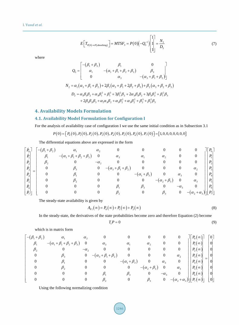
(7)

where

( )( )

( )

1 2 1

3 1 1 1 2 3 3

3 3 1 2

0

0Q

β β βα α β β β β

α α β β

− + = − + + + − + +

( ) ( ) ( )2 1 3 1 2 1 3 1 2 3 2 3 2 32 2N α α β β β α β β β β α β β= + + + + + + + + + 2 3 2 2 2

2 1 1 2 3 1 1 1 2 3 1 2 1 2 1 32 2 3 2

1 2 3 1 3 2 1 2 3 2 2 2 3

3 2 3

2

D α β β α β β β β α β β β β β β

β β β α α β α β α β β β β

= + + + + + +

+ + + + + +

4. Availability Models Formulation 4.1. Availability Model Formulation for Configuration I For the analysis of availability case of configuration I we use the same initial condition as in Subsection 3.1

( ) ( ) ( ) ( ) ( ) ( ) ( ) ( ) ( ) [ ]0 1 2 3 4 5 6 70 0 , 0 , 0 , 0 , 0 , 0 , 0 , 0 1,0,0,0,0,0,0,0P P P P P P P P P= =

The differential equations above are expressed in the form

( )( )

( )( )

( )

( )

1 2 1 20

1 1 1 2 3 3 1 21

2 22

3 3 1 2 23

1 1 3 34

2 2 3 35

1 3 36

2 3 2 37

0 0 0 0 00 0 0

0 0 0 0 0 00 0 0 0 00 0 0 0 00 0 0 0 00 0 0 0 00 0 0 0 0

PPPPPPPP

β β α αβ α β β β α α αβ α

β α β β αβ α β αβ α β α

β β αβ β α α

− + − + + + −

− + + = − +

− + − − +

0

1

2

3

4

5

6

7

PPPPPPPP

The steady-state availability is given by

( ) ( ) ( ) ( )1 0 1 3VA P P P∞ = ∞ + ∞ + ∞ (8)

In the steady-state, the derivatives of the state probabilities become zero and therefore Equation (2) become

1 0T P = (9)

which is in matrix form

( )( )

( )( )

( )

( )

( )( )( )( )( )( )( )( )

1 2 1 2 0

1 1 1 2 3 3 1 2 1

2 2 2

3 3 1 2 2 3

1 1 3 3 4

2 2 3 3 5

1 3 3 6

2 3 2 3 7

0 0 0 0 00 0 0

0 0 0 0 0 00 0 0 0 00 0 0 0 00 0 0 0 00 0 0 0 00 0 0 0 0

PPPPPPPP

β β α αβ α β β β α α αβ α

β α β β αβ α β αβ α β α

β β αβ β α α

− + ∞ − + + + ∞ − ∞

− + + ∞ − + ∞

− + ∞ − ∞ − + ∞

00000000

=

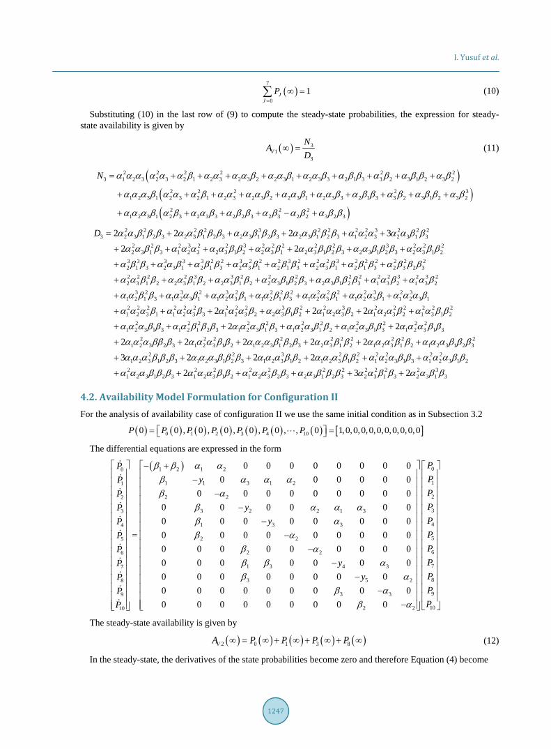
Using the following normalizing condition

I. Yusuf et al.

1247

( )7

01J

JP

=

∞ =∑ (10)

Substituting (10) in the last row of (9) to compute the steady-state probabilities, the expression for steady- state availability is given by

( ) 31

3V

NA

D∞ = (11)

( )( )( )

2 2 2 2 2 23 1 2 3 2 3 2 1 2 3 2 3 2 2 3 1 2 3 3 2 1 3 3 2 3 1 2 3 2

2 2 2 2 31 2 3 1 2 3 2 1 2 3 2 3 2 2 3 1 2 3 3 2 1 3 3 2 3 1 2 3 2

2 2 21 2 3 1 2 3 2 3 3 2 2 3 2 3 2 2 3 2 3

N α α α α α α β α α α α β α α β α α β α β β α β α β β α β

α α α β α α α β α α α α β α α β α α β α β β α β α β β α β

α α α β α β α α β α β β α β α β α β β

= + + + + + + + + +

+ + + + + + + + + +

+ + + + − +

2 2 2 2 3 2 2 2 2 3 2 2 23 2 3 1 2 3 2 3 1 2 3 2 3 1 2 3 2 3 1 2 3 1 2 3 2 3 1 3

2 2 2 3 2 2 3 2 2 2 2 2 3 2 2 22 3 1 3 1 2 3 2 3 1 2 2 3 1 2 3 1 2 3 2 3 1 2 3 2 3 1 2

3 3 3 3 3 2 2 3 2 22 1 3 2 3 1 2 1 3 2 3 1

2 2 2 3

2 2

D α α β β β α α β β β α α β β β α α β β β α α α α α β β

α α β β α α α α α β β α α β α α β β β α α β β β α α β β

α β β α α β α β β α α β α

= + + + + +

+ + + + + + +

+ + + + + 2 3 2 2 2 3 2 2 2 2 2 22 1 3 2 3 1 2 1 3 2 3 2 3

2 2 2 2 3 3 2 2 2 2 2 2 2 3 2 3 22 3 1 2 2 3 1 2 2 3 1 2 2 3 1 2 3 2 3 1 2 3 1 3 2 1 3 2

3 2 3 2 3 2 2 2 2 2 2 2 2 3 2 31 2 1 3 1 2 3 1 1 2 3 1 1 2 1 3 1 2 3 1 1 2 3 1 1 2 3 1

β β α α β α β β α β β β

α α β β α α β β α α β β α α β β β α α β β β α α β α α β

α α β β α α α β α α α β α α β β α α α β α α α β α α α β

+ + +

+ + + + + + +

+ + + + + + +

+ 2 2 2 2 2 2 2 2 2 3 2 2 3 2 2 2 2 2 21 2 3 1 1 2 3 3 1 2 3 2 2 3 1 2 1 2 3 2 1 2 3 2 1 3 1 2

2 2 2 2 2 2 2 2 2 2 21 2 3 1 3 1 2 1 2 3 1 2 3 1 3 1 2 3 1 2 1 2 3 1 3 1 2 3 1 3

2 2 21 2 3 2 3 1 2 3 1 2 1 2 3

2 2 2

2 2

2 2 2

α α α β α α α β α α α β α α β β α α α β α α α β α α β β

α α α β β α α β β β α α α β β α α α β β α α α β β α α α β β

α α α ββ β α α α β β α α α β

+ + + + + +

+ + + + + +

+ + + 2 2 2 2 2 2 21 2 3 2 3 1 2 1 2 3 1 2 1 2 3 1 2 3

2 2 3 2 2 2 2 2 21 2 3 1 2 3 1 2 3 1 2 3 1 2 3 1 2 1 2 3 1 2 1 2 3 1 3 1 2 3 1 2

2 2 2 2 2 2 2 2 2 21 2 3 1 2 3 1 2 3 1 2 1 2 3 2 3 2 3 1 2 3 2 3 1 3

2 2

3 2 2 2

2 3 2

β β α α β β α α α β β α α α β β β

α α α β β β α α α β β β α α α β β α α α β β α α α β β α α α β β

α α α β β β α α α β β α α α β β α α β β β α α β β α

+ + +

+ + + + + +

+ + + + + + 2 32 3 1 3α β β

4.2. Availability Model Formulation for Configuration II For the analysis of availability case of configuration II we use the same initial condition as in Subsection 3.2

( ) ( ) ( ) ( ) ( ) ( ) ( ) [ ]0 1 2 3 4 100 0 , 0 , 0 , 0 , 0 , , 0 1,0,0,0,0,0,0,0,0,0,0P P P P P P P= =

The differential equations are expressed in the form

( )1 2 1 20

1 1 3 1 21

2 22

3 2 2 1 33

1 3 34

2 25

2 26

1 3 4 37

8

9

10

0 0 0 0 0 0 0 00 0 0 0 0 0

0 0 0 0 0 0 0 0 00 0 0 0 0 00 0 0 0 0 0 0 00 0 0 0 0 0 0 0 00 0 0 0 0 0 0 0 00 0 0 0 0 0 00 0 0

PyP

PyP

yPPP

yPPPP

β β α αβ α α αβ α

β α α αβ αβ α

β αβ β αβ

− + − −

− −

= − − −

0

1

2

3

4

5

6

7

83 5 2

93 3

102 2

0 0 0 0 00 0 0 0 0 0 0 0 00 0 0 0 0 0 0 0 0

PPPPPPPPPyPP

αβ α

β α

− −

−

The steady-state availability is given by

( ) ( ) ( ) ( ) ( )2 0 1 3 8VA P P P P∞ = ∞ + ∞ + ∞ + ∞ (12)

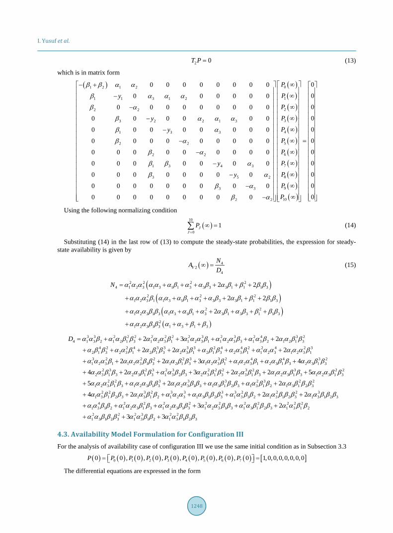
In the steady-state, the derivatives of the state probabilities become zero and therefore Equation (4) become

I. Yusuf et al.

1248

2 0T P = (13)

which is in matrix form

( )1 2 1 2

1 1 3 1 2

2 2

3 2 2 1 3

1 3 3

2 2

2 2

1 3 4 3

3 5 2

3 3

2 2

0 0 0 0 0 0 0 0

0 0 0 0 0 0

0 0 0 0 0 0 0 0 0

0 0 0 0 0 0

0 0 0 0 0 0 0 0

0 0 0 0 0 0 0 0 0

0 0 0 0 0 0 0 0 0

0 0 0 0 0 0 0

0 0 0 0 0 0 0 0

0 0 0 0 0 0 0 0 0

0 0 0 0 0 0 0 0 0

y

y

y

y

y

β β α α

β α α α

β α

β α α α

β α

β α

β α

β β α

β α

β α

β α

− +

− − − −

−

− − − −

−

( )( )( )( )( )( )( )( )( )( )( )

0

1

2

3

4

5

6

7

8

9

10

0

0

0

0

0

0

0

0

0

0

0

P

P

P

P

P

P

P

P

P

P

P

∞

∞ ∞ ∞ ∞

=∞ ∞ ∞ ∞ ∞

∞

Using the following normalizing condition

( )10

01J

JP

=

∞ =∑ (14)

Substituting (14) in the last row of (13) to compute the steady-state probabilities, the expression for steady- state availability is given by

( ) 42

4V

NAD

∞ = (15)

( )( )( )( )

2 2 2 24 1 2 3 1 3 1 1 3 3 3 3 1 1 1 3

2 2 21 2 3 1 1 3 1 1 3 3 3 3 1 1 1 3

2 21 2 3 1 3 1 3 1 1 3 3 1 3 3 1 1 3

21 2 3 1 3 1 3 1 3

2 2

2 2

2

N α α α α α α β α α β α β β β β

α α α β α α α β α α β α β β β β

α α α β β α α α β α α β α β β β β

α α α β β α α β β

= + + + + + +

+ + + + + + +

+ + + + + + +

+ + + + 3 3 2 2 2 2 2 2 2 3 2 3 2 4 3 2

4 1 3 2 1 2 1 3 1 2 3 1 1 2 3 1 1 2 3 3 1 3 2 1 2 1 34 2 2 4 3 3 3 3 2 4 4 2 2 4 2 3

2 1 3 2 3 1 2 1 3 2 3 1 2 1 3 2 3 1 1 2 3 1 2 3 13 2 2 2 2 31 2 3 1 1 2 3 1 3 1 2 1 3 1 2

2 3 2

2 2 2

2 2 3

D α α β α α β β α α α β α α α β α α α β α α β α α β β

α β β α α β α β β α α β α β β α α β α α α α α α β

α α α β α α α β β α α β β α α

= + + + + + +

+ + + + + + + +

+ + + + 3 2 4 4 3 23 1 1 2 3 1 2 3 1 3 2 3 1 3

2 3 2 3 2 3 2 2 2 3 2 3 2 22 3 1 3 2 3 1 3 1 3 2 3 2 3 1 3 2 3 1 3 1 2 3 1 3 1 2 3 1 3

2 2 3 3 3 2 3 21 2 3 1 3 1 2 3 1 3 1 2 3 1 3 1 3 1 2 3 1 3 1 2 1 3 1 2 3

4

4 2 3 2 2 5

5 2 2

α β α α α β α α β β α α β β

α α β β α α β β α α β β α α β β α α β β α α α β β α α α β β

α α α β β α α α β β α α α β β α α β β β α α β β α α β β β

+ + +

+ + + + + + +

+ + + + + + 2

2 2 3 2 3 3 3 3 2 2 2 31 3 1 2 3 1 3 1 2 1 2 3 1 3 1 2 3 1 3 1 2 1 3 1 2 3 1 3 1 2 3

4 2 2 2 2 2 2 2 2 2 2 21 3 1 2 1 2 3 1 3 1 2 3 1 3 1 2 3 1 3 1 3 1 2 3 1 3 1 22 2 2 3 2 21 3 1 2 3 1 3 1 2 1 3 1 2

4 2 2 2

3 2

3 3

α α β β β α α β β α α α α α β β β α α β β α α β β β α α β β β

α α β β α α α β β α α α β β α α α β β α α β β β α α β β

α α β β β α α β β α α β β β

+ + + + + + +

+ + + + + +

+ + + 3

4.3. Availability Model Formulation for Configuration III For the analysis of availability case of configuration III we use the same initial condition as in Subsection 3.3

( ) ( ) ( ) ( ) ( ) ( ) ( ) ( ) ( ) [ ]0 1 2 3 4 5 6 70 0 , 0 , 0 , 0 , 0 , 0 , 0 , 0 1,0,0,0,0,0,0,0P P P P P P P P P= =

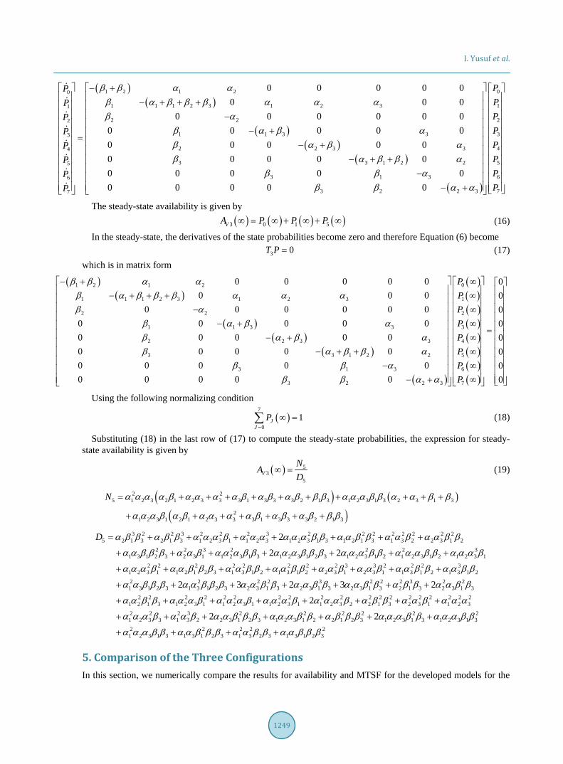
The differential equations are expressed in the form

I. Yusuf et al.

1249

( )( )

( )( )

( )

( )

1 2 1 20

1 1 1 2 3 1 2 31

2 22

1 1 3 33

2 2 3 34

3 3 1 2 25

3 1 36

3 2 2 37

0 0 0 0 00 0 0

0 0 0 0 0 00 0 0 0 00 0 0 0 00 0 0 0 00 0 0 0 00 0 0 0 0

PPPPPPPP

β β α αβ α β β β α α αβ α

β α β αβ α β αβ α β β α

β β αβ β α α

− + − + + + −

− + = − +

− + + − − +

0

1

2

3

4

5

6

7

PPPPPPPP

The steady-state availability is given by

( ) ( ) ( ) ( )3 0 1 5VA P P P∞ = ∞ + ∞ + ∞ (16)

In the steady-state, the derivatives of the state probabilities become zero and therefore Equation (6) become

3 0T P = (17) which is in matrix form

( )( )

( )( )

( )

( )

( )( )( )( )( )( )( )( )

1 2 1 2 0

1 1 1 2 3 1 2 3 1

2 2 2

1 1 3 3 3

2 2 3 3 4

3 3 1 2 2 5

3 1 3 6

3 2 2 3 7

0 0 0 0 00 0 0

0 0 0 0 0 00 0 0 0 00 0 0 0 00 0 0 0 00 0 0 0 00 0 0 0 0

PPPPPPPP

β β α αβ α β β β α α αβ α

β α β αβ α β αβ α β β α

β β αβ β α α

− + ∞ − + + + ∞ − ∞

− + ∞ − + ∞

− + + ∞ − ∞ − + ∞

00000000

=

Using the following normalizing condition

( )7

01J

JP

=

∞ =∑ (18)

Substituting (18) in the last row of (17) to compute the steady-state probabilities, the expression for steady- state availability is given by

( ) 53

5V

NA

D∞ = (19)

( ) ( )

( )

2 25 1 2 3 2 1 2 3 3 3 1 3 3 3 2 1 3 1 2 3 1 3 2 3 1 3

21 2 3 1 2 1 2 3 3 3 1 3 3 3 2 1 3

N α α α α β α α α α β α β α β β β α α α β β α α β β

α α α β α β α α α α β α β α β β β

= + + + + + + + + + +

+ + + + + + +

3 2 2 3 2 2 2 3 2 2 2 2 2 2 2 25 2 1 3 2 1 3 1 2 3 1 1 2 3 1 2 3 1 3 1 2 1 3 1 3 2 2 3 1 2

2 2 3 2 2 2 31 3 1 2 3 2 3 1 1 2 3 1 3 1 2 3 1 2 3 1 2 3 1 2 1 2 3 1 2 1 2 3 1

2 2 2 2 21 2 3 1 1 2 1 2 3 1 3 1

2

2 2

D α β β α β β α α α β α α α α α α β β α α β β α α β α α β β

α α β β β α α β α α α β β α α α β β β α α α β β α α α β β α α α β

α α α β α α β β β α α β β

= + + + + + + +

+ + + + + + +

+ + + 2 2 2 3 3 2 2 2 32 1 3 1 2 2 3 1 2 3 1 1 3 1 2 1 3 1 2

2 2 2 2 3 2 2 2 3 2 21 3 1 2 3 1 3 1 2 3 2 3 1 3 2 3 1 3 2 3 1 3 2 1 3 2 3 1 3

2 2 2 2 2 2 2 2 2 2 2 2 21 2 1 3 1 2 3 1 1 2 3 1 1 2 3 1 1 2 3 2 2 1 3

2 3 2 3 2

2

α α β β α α β α α β α α β β α α β β

α α β β β α α β β β α α β β α α β β α α β β α β β α α β β

α α β β α α α β α α α β α α α β α α α β α β β α

+ + + + +

+ + + + + + +

+ + + + + + + 2 2 2 2 2 22 3 1 1 2 3

2 2 2 3 2 2 2 2 2 21 2 3 3 1 3 2 2 3 1 2 3 1 2 3 1 2 2 1 2 3 1 2 3 1 3 1 2 3 1 32 2 2 2 21 2 3 1 3 1 3 1 2 3 1 3 2 3 1 3 1 2 3

2 2

α β α α α

α α α β α α β α α β β β α α α β β α β β β α α α β β α α α β β

α α α β β α α β β β α α β β α α β β β

+

+ + + + + + +

+ + + +

5. Comparison of the Three Configurations In this section, we numerically compare the results for availability and MTSF for the developed models for the

I. Yusuf et al.

1250

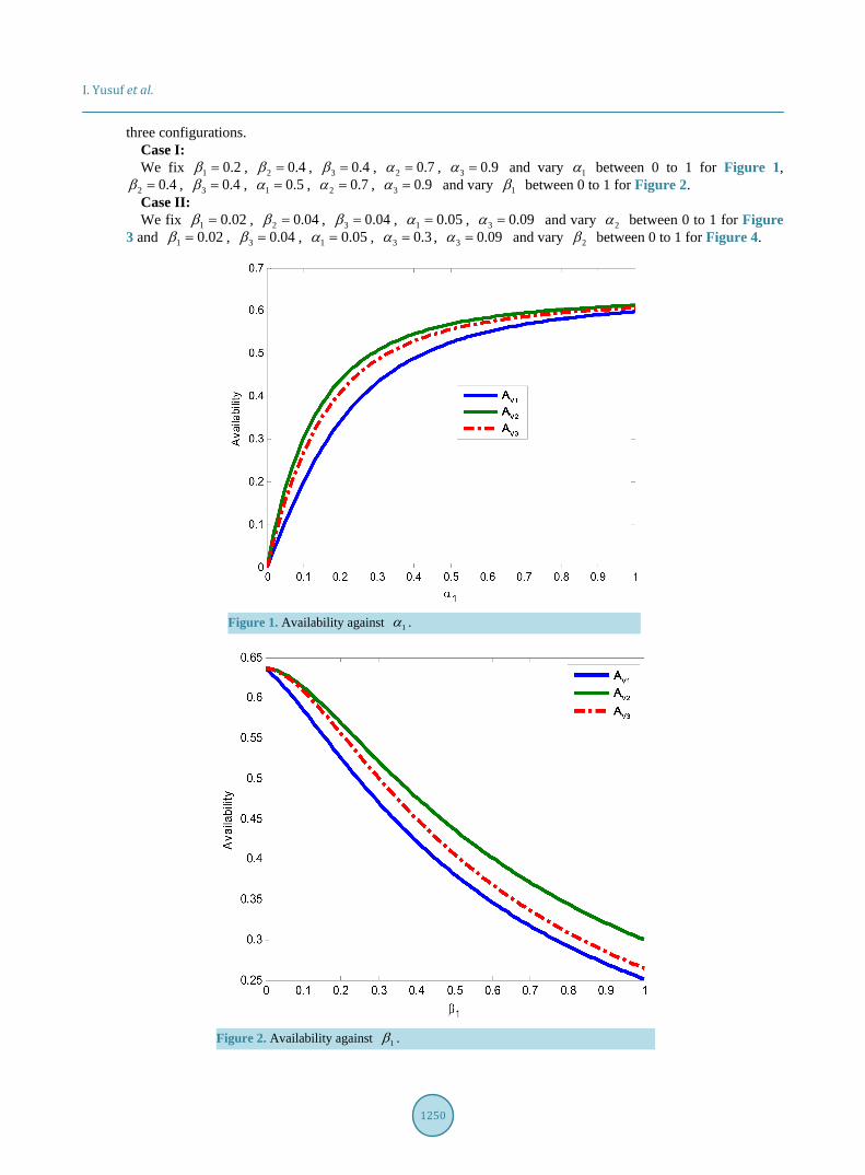
three configurations. Case I: We fix 1 0.2β = , 2 0.4β = , 3 0.4β = , 2 0.7α = , 3 0.9α = and vary 1α between 0 to 1 for Figure 1,

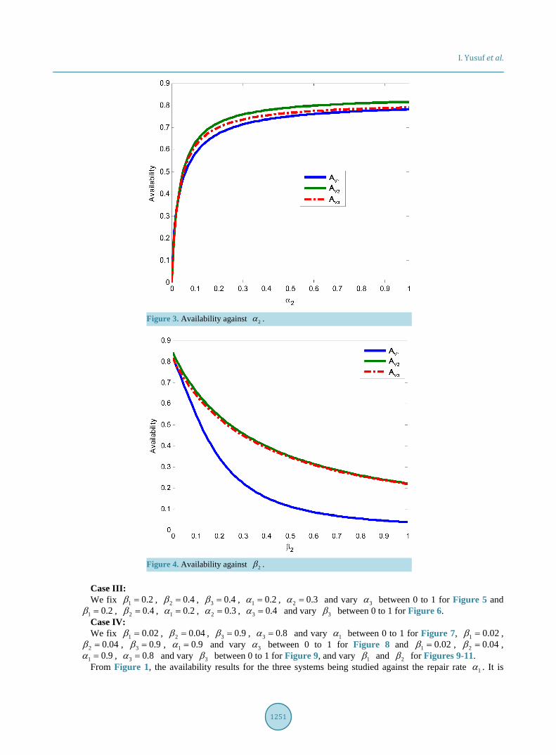
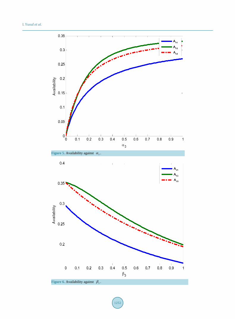
2 0.4β = , 3 0.4β = , 1 0.5α = , 2 0.7α = , 3 0.9α = and vary 1β between 0 to 1 for Figure 2. Case II: We fix 1 0.02β = , 2 0.04β = , 3 0.04β = , 1 0.05α = , 3 0.09α = and vary 2α between 0 to 1 for Figure

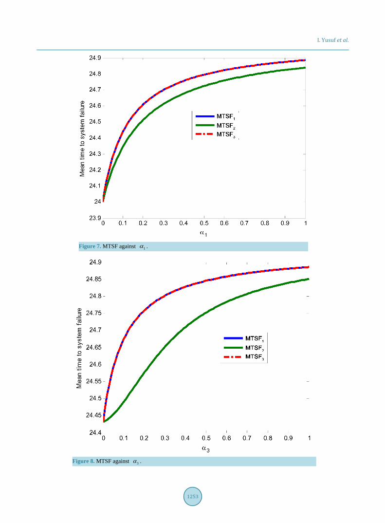
3 and 1 0.02β = , 3 0.04β = , 1 0.05α = , 3 0.3α = , 3 0.09α = and vary 2β between 0 to 1 for Figure 4.

Figure 1. Availability against 1α .

Figure 2. Availability against 1β .

I. Yusuf et al.

1251

Figure 3. Availability against 2α .

Figure 4. Availability against 2β .

Case III: We fix 1 0.2β = , 2 0.4β = , 3 0.4β = , 1 0.2α = , 2 0.3α = and vary 3α between 0 to 1 for Figure 5 and

1 0.2β = , 2 0.4β = , 1 0.2α = , 2 0.3α = , 3 0.4α = and vary 3β between 0 to 1 for Figure 6. Case IV: We fix 1 0.02β = , 2 0.04β = , 3 0.9β = , 3 0.8α = and vary 1α between 0 to 1 for Figure 7, 1 0.02β = ,

2 0.04β = , 3 0.9β = , 1 0.9α = and vary 3α between 0 to 1 for Figure 8 and 1 0.02β = , 2 0.04β = , 1 0.9α = , 3 0.8α = and vary 3β between 0 to 1 for Figure 9, and vary 1β and 2β for Figures 9-11. From Figure 1, the availability results for the three systems being studied against the repair rate 1α . It is

I. Yusuf et al.

1252

Figure 5. Availability against 3α .

Figure 6. Availability against 3β .

I. Yusuf et al.

1253

Figure 7. MTSF against 1α .

Figure 8. MTSF against 3α .

I. Yusuf et al.

1254

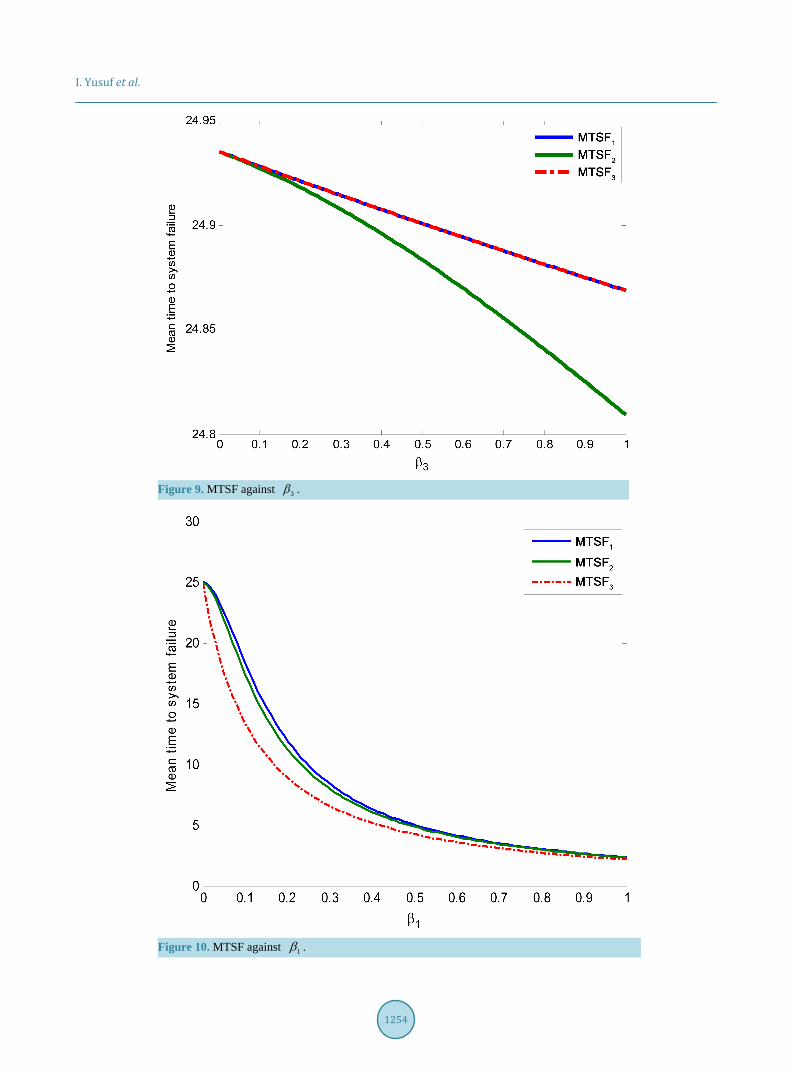
Figure 9. MTSF against 3β .

Figure 10. MTSF against 1β .

I. Yusuf et al.

1255

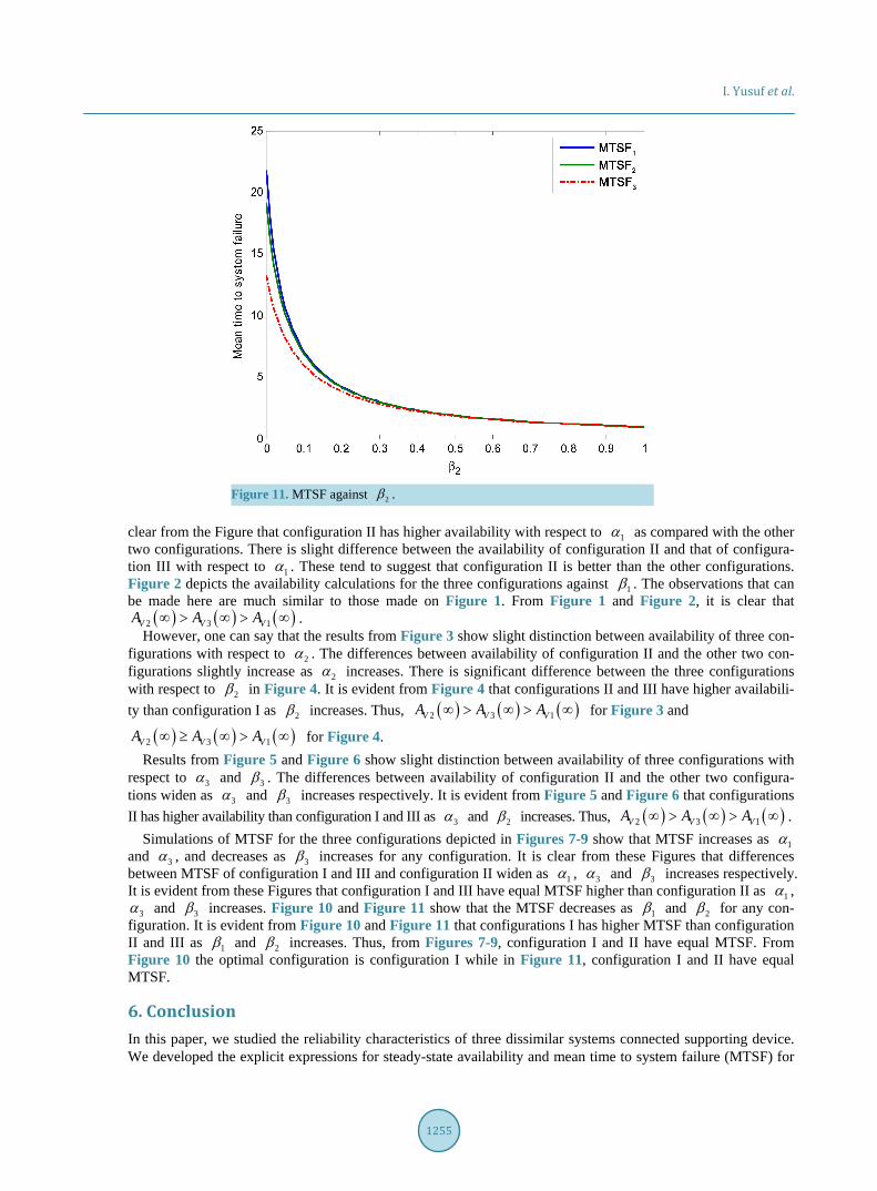
Figure 11. MTSF against 2β .

clear from the Figure that configuration II has higher availability with respect to 1α as compared with the other two configurations. There is slight difference between the availability of configuration II and that of configura-tion III with respect to 1α . These tend to suggest that configuration II is better than the other configurations. Figure 2 depicts the availability calculations for the three configurations against 1β . The observations that can be made here are much similar to those made on Figure 1. From Figure 1 and Figure 2, it is clear that

( ) ( ) ( )2 3 1V V VA A A∞ > ∞ > ∞ . However, one can say that the results from Figure 3 show slight distinction between availability of three con-

figurations with respect to 2α . The differences between availability of configuration II and the other two con-figurations slightly increase as 2α increases. There is significant difference between the three configurations with respect to 2β in Figure 4. It is evident from Figure 4 that configurations II and III have higher availabili- ty than configuration I as 2β increases. Thus, ( ) ( ) ( )2 3 1V V VA A A∞ > ∞ > ∞ for Figure 3 and

( ) ( ) ( )2 3 1V V VA A A∞ ≥ ∞ > ∞ for Figure 4. Results from Figure 5 and Figure 6 show slight distinction between availability of three configurations with

respect to 3α and 3β . The differences between availability of configuration II and the other two configura-tions widen as 3α and 3β increases respectively. It is evident from Figure 5 and Figure 6 that configurations II has higher availability than configuration I and III as 3α and 2β increases. Thus, ( ) ( ) ( )2 3 1V V VA A A∞ > ∞ > ∞ .

Simulations of MTSF for the three configurations depicted in Figures 7-9 show that MTSF increases as 1α and 3α , and decreases as 3β increases for any configuration. It is clear from these Figures that differences between MTSF of configuration I and III and configuration II widen as 1α , 3α and 3β increases respectively. It is evident from these Figures that configuration I and III have equal MTSF higher than configuration II as 1α ,

3α and 3β increases. Figure 10 and Figure 11 show that the MTSF decreases as 1β and 2β for any con-figuration. It is evident from Figure 10 and Figure 11 that configurations I has higher MTSF than configuration II and III as 1β and 2β increases. Thus, from Figures 7-9, configuration I and II have equal MTSF. From Figure 10 the optimal configuration is configuration I while in Figure 11, configuration I and II have equal MTSF.

6. Conclusion In this paper, we studied the reliability characteristics of three dissimilar systems connected supporting device. We developed the explicit expressions for steady-state availability and mean time to system failure (MTSF) for

I. Yusuf et al.

1256

each configuration and performed comparative analysis numerically to determine the optimal configuration. It is evident from Figures 1-6 that configuration II is optimal configuration using steady-state availability while us-ing MTSF, the optimal configuration depends on the values of 1α , 3α , 1β , 2β and 3β . The present study will help the engineers and designers to develop sophisticated models and to design more critical system in in-terest of human kind.

References [1] Khatab, A., Nahas, N. and Nourelfath, M. (2009) Availability of k-out-of-n: G Systems with Non Identical Compo-

nents Subject to Repair Priorities. Reliability Engineering & System Safety, 94, 142-151. http://dx.doi.org/10.1016/j.ress.2008.02.017

[2] Fathabadi, H.S. and Khodaei, M. (2012) Reliability Evaluation of Network Flows with Stochastic Capacity and Cost Constraint. International Journal of Mathematics in Operational Research, 4, 439-452. http://dx.doi.org/10.1504/IJMOR.2012.048904

[3] Khalili-Damghani, K. and Amiri, M. (2012) Solving Binary-State Multi-Objective Reliability Redundancy Allocation Seriesparallel Problem Using Efficient Epsilon Constraint, Multi-Start Partial Bound Enumeration Algorithm, and DEA. Reliability Engineering and System Safety, 103, 35-44. http://dx.doi.org/10.1016/j.ress.2012.03.006

[4] Khalili-Damghani, K., Abtahi, A.R., and Tavana, M. (2013) A New Multi-Objective Particle Swarm Optimization Method for Solving Reliability Redundancy Allocation Problems. Reliability Engineering and System Safety, 111, 58- 75. http://dx.doi.org/10.1016/j.ress.2012.10.009

[5] Wang, K.-H., Yen, T.-C. and Fang, Y.-C. (2012) Comparison of Availability between Two Systems with Warm Standby Units and Different Imperfect Coverage. Quality Technology and Quantitative Management, 9, 265-282

[6] Srinivasan, S.K. and Subramanian, R. (2006) Reliability Analysis of a Three Unit Warm Standby Redundant System with Repair. Annals of Operations Research, 143, 227-235. http://dx.doi.org/10.1007/s10479-006-7384-z

[7] Singh, V.V., Singh, B., Mangeyram and Goel, C.K. (2010) Availability Analysis of a System Having Three Units Su-per Priority, Priority and Ordinary under Peemmptive Resume Repair Policy. International Journal of Reliability and Applications, 11, 41-53.

[8] Singh, V.V. and Rawal, D.K. (2011) Availability Analysis of a System Having Two Units in Series Configuration with Controller and Human Failure under Different Repair Policies. International Journal of Scientific and Engineering Re-search, 2, 1-9.

[9] Yusuf, I. (2013) Comparison of Some Reliability Characteristics between Redundant Systems Requiring Supporting Units for Their Operation. Journal of Mathematical and Computational Sciences, 3, 216-232.

[10] Yusuf, I. (2014) Comparative Analysis of Profit between Three Dissimilar Repairable Redundant Systems Using Sup-porting External Device for Operation. Journal of Industrial Engineering International, 10, 2-9. http://dx.doi.org/10.1007/s40092-014-0077-3

[11] Wang, K.H. and Kuo, C.C. (2000) Cost and Probabilistic Analysis of Series Systems with Mixed Standby Components. Applied Mathematical Modelling, 24, 957-967. http://dx.doi.org/10.1016/S0307-904X(00)00028-7

[12] Wang, K., Hsieh, C. and Liou, C. (2006) Cost Benefit Analysis of Series Systems with Cold Standby Components and a Repairable Service Station. Journal of Quality Technology and Quantitative Management, 3, 77-92.