RELIABILITY OF TEST METHODS FOR METALLIC PRODUCTS - FINAL ...dwi.defra.gov.uk/research/.../reports/DWI70_2_151_testmethods.pdf · Reliability of test methods for metallic products

DETR/DWI DWI 6090 DECEMBER 2002

Reliability of test methods for metallic products - Final Report to the Drinking Water Inspectorate

Final Report to the Department for Environment, Food and Rural Affairs

RELIABILITY OF TEST METHODS FOR METALLIC PRODUCTS - FINAL REPORT TO THE DRINKING WATER INSPECTORATE

Final Report to the Department for Environment, Food and Rural Affairs

Report No: DETR/DWI 6090

December 2002

Authors: R J Oliphant, E B Glennie

Contract Manager: J Trew

Contract No: 12969-0

DETR Reference No: 70/2/151

Contract Duration: December 2001 - December 2002

Any enquiries relating to this report should be referred to the Contract Manager at the following address: WRc-NSF plc, Henley Road, Medmenham, Marlow, Buckinghamshire SL7 2HD. Telephone: + 44 (0) 1491 636500 Fax: + 44 (0) 1491 636501

This report has the following distribution: External: DWI

Internal: Authors and Contract Manager

RELIABILITY OF TEST METHODS FOR METALLIC PRODUCTS - FINAL REPORT TO THE DRINKING WATER INSPECTORATE

i

EXECUTIVE SUMMARY

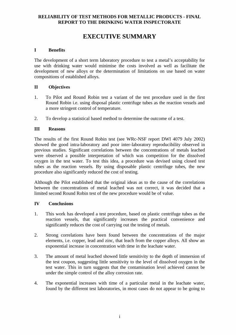
I Benefits

The development of a short term laboratory procedure to test a metal’s acceptability for use with drinking water would minimise the costs involved as well as facilitate the development of new alloys or the determination of limitations on use based on water compositions of established alloys.

II Objectives

1. To Pilot and Round Robin test a variant of the test procedure used in the first Round Robin i.e. using disposal plastic centrifuge tubes as the reaction vessels and a more stringent control of temperature.

2. To develop a statistical based method to determine the outcome of a test.

III Reasons

The results of the first Round Robin test (see WRc-NSF report DWI 4079 July 2002) showed the good intra-laboratory and poor inter-laboratory reproducibility observed in previous studies. Significant correlations between the concentrations of metals leached were observed a possible interpretation of which was competition for the dissolved oxygen in the test water. To test this idea, a procedure was devised using closed test tubes as the reaction vessels. By using disposable plastic centrifuge tubes, the new procedure also significantly reduced the cost of testing.

Although the Pilot established that the original ideas as to the cause of the correlations between the concentrations of metal leached was not correct, it was decided that a limited second Round Robin test of the new procedure would be of value.

IV Conclusions

1. This work has developed a test procedure, based on plastic centrifuge tubes as the reaction vessels, that significantly increases the practical convenience and significantly reduces the cost of carrying out the testing of metals.

2. Strong correlations have been found between the concentrations of the major elements, i.e. copper, lead and zinc, that leach from the copper alloys. All show an exponential increase in concentration with time in the leachate water.

3. The amount of metal leached showed little sensitivity to the depth of immersion of the test coupon, suggesting little sensitivity to the level of dissolved oxygen in the test water. This in turn suggests that the contamination level achieved cannot be under the simple control of the alloy corrosion rate.

4. The exponential increases with time of a particular metal in the leachate water, found by the different test laboratories, in most cases do not appear to be going to

ii

the same equilibrium value. This suggests that the contamination level achieved cannot be under the simple control of the solubility of the corrosion product formed.

5. The levels of copper and zinc leached in the tests were so far below their respective PCV’s that the acceptability for these elements of the alloys tested could be made unambiguously. This was not the case for lead.

6. Although the differences between measured lead concentrations at the three laboratories were considerable, a statistical procedure to decide the outcome of the test, that takes these ‘between laboratory’ differences into account, can be suggested.

iii

CONTENTS Page

EXECUTIVE SUMMARY i

LIST OF TABLES iii

LIST OF FIGURES iv

1. INTRODUCTION 1

2. RESULTS 3

3. DISCUSSION 7

4. CONCLUSIONS 11

APPENDICES

APPENDIX A REPORT ON THE EFFECT OF DEPTH OF IMMERSION STUDY – SECOND PILOT USING MODIFIED DD 256:2002 PROCEDURE 21

APPENDIX B METHOD FOR BS7766 ROUND-ROBIN 2 EXERCISE 27 APPENDIX C RESULTS 31 APPENDIX D ANALYSIS OF VARIANCE: GENSTAT OUTPUT 37 APPENDIX E DERIVATION OF TEST OUTCOME RULES 41

LIST OF TABLES

Table 1 Test water analyses 3 Table 2a Summary of Stagnation Results - Average metal concentration

µg/l 4 Table 2b Summary of Stagnation Results - Average metal concentration

µg-equivalents/l 5

Table 3 Sixteen hour stagnation concentrations for Lead 6 Table 4 Weighted average stagnation time concentrations for Lead

(µg/l) after a 16 day aging period 8 Table 5 Decisions based on test results 9 Table E.1 Estimation of between laboratory variability 41

Page

iv

LIST OF FIGURES

Figure 1 Copper stagnation concentrations – average of 5 replicates 12 Figure 2 Lead stagnation concentrations – average of 5 replicates 13 Figure 3 Zinc stagnation concentrations – average of 5 replicates 14 Figure 4 Sum of 3 metals gm equivalents – average of 5 replicates 15 Figure 5 Correlations between Levels of Copper and Zinc Leaching 16 Figure 6 Copper + Zinc versus Lead Leaching 17 Figure 7 Copper, 2nd Round robin, 24 hour stagnation concentrations 18 Figure 8 Lead, 2nd Round Robin, 24 hour stagnation concentrations 18 Figure 9 Zinc, 2nd Round Robin, 24 hour stagnation concentrations 19 Figure 10 ITS Lead 16 hour stagnation concentrations 19 Figure 11 WRC-NSF Lead 16 hour stagnation concentrations 20 Figure 12 TW Lead 16 hour stagnation concentrations 20

1

1. INTRODUCTION

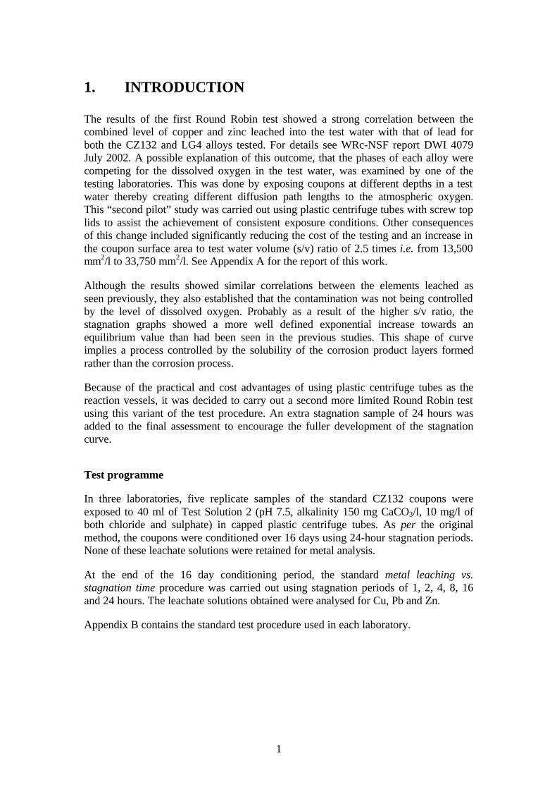
The results of the first Round Robin test showed a strong correlation between the combined level of copper and zinc leached into the test water with that of lead for both the CZ132 and LG4 alloys tested. For details see WRc-NSF report DWI 4079 July 2002. A possible explanation of this outcome, that the phases of each alloy were competing for the dissolved oxygen in the test water, was examined by one of the testing laboratories. This was done by exposing coupons at different depths in a test water thereby creating different diffusion path lengths to the atmospheric oxygen. This “second pilot” study was carried out using plastic centrifuge tubes with screw top lids to assist the achievement of consistent exposure conditions. Other consequences of this change included significantly reducing the cost of the testing and an increase in the coupon surface area to test water volume (s/v) ratio of 2.5 times i.e. from 13,500 mm2/l to 33,750 mm2/l. See Appendix A for the report of this work.

Although the results showed similar correlations between the elements leached as seen previously, they also established that the contamination was not being controlled by the level of dissolved oxygen. Probably as a result of the higher s/v ratio, the stagnation graphs showed a more well defined exponential increase towards an equilibrium value than had been seen in the previous studies. This shape of curve implies a process controlled by the solubility of the corrosion product layers formed rather than the corrosion process.

Because of the practical and cost advantages of using plastic centrifuge tubes as the reaction vessels, it was decided to carry out a second more limited Round Robin test using this variant of the test procedure. An extra stagnation sample of 24 hours was added to the final assessment to encourage the fuller development of the stagnation curve.

Test programme

In three laboratories, five replicate samples of the standard CZ132 coupons were exposed to 40 ml of Test Solution 2 (pH 7.5, alkalinity 150 mg CaCO3/l, 10 mg/l of both chloride and sulphate) in capped plastic centrifuge tubes. As per the original method, the coupons were conditioned over 16 days using 24-hour stagnation periods. None of these leachate solutions were retained for metal analysis.

At the end of the 16 day conditioning period, the standard metal leaching vs. stagnation time procedure was carried out using stagnation periods of 1, 2, 4, 8, 16 and 24 hours. The leachate solutions obtained were analysed for Cu, Pb and Zn.

Appendix B contains the standard test procedure used in each laboratory.

2

3

2. RESULTS

Average stagnation curves of five replicates

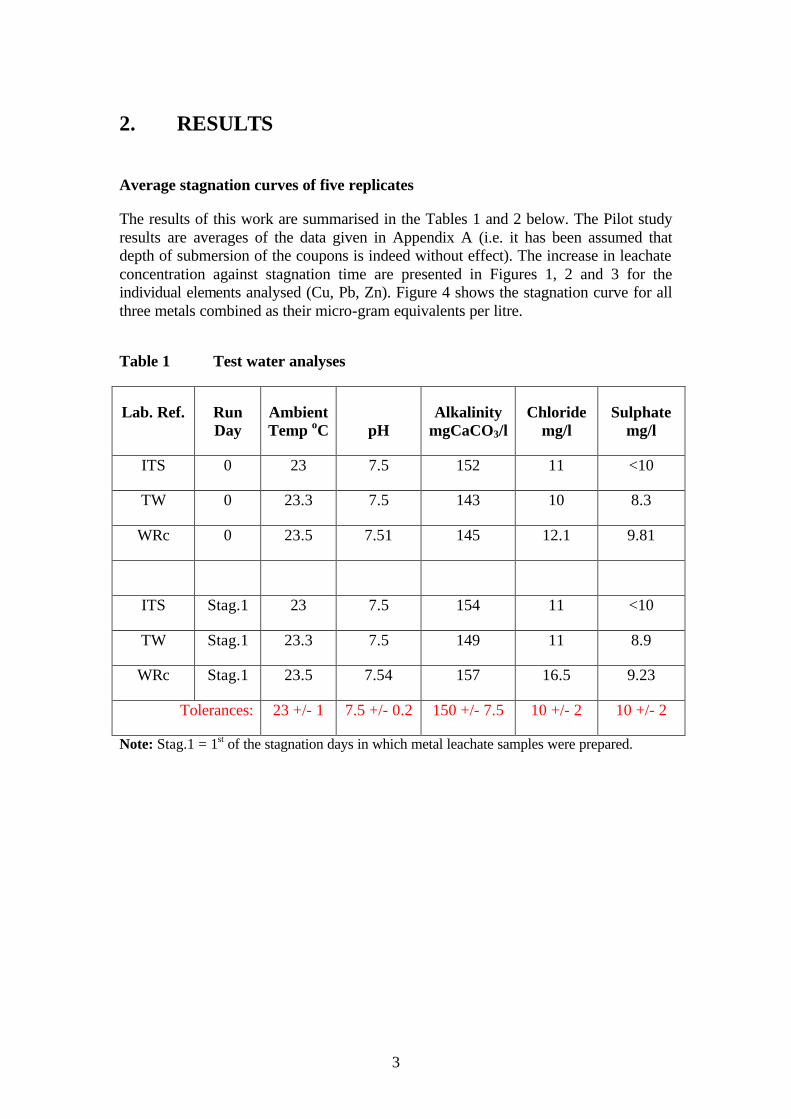
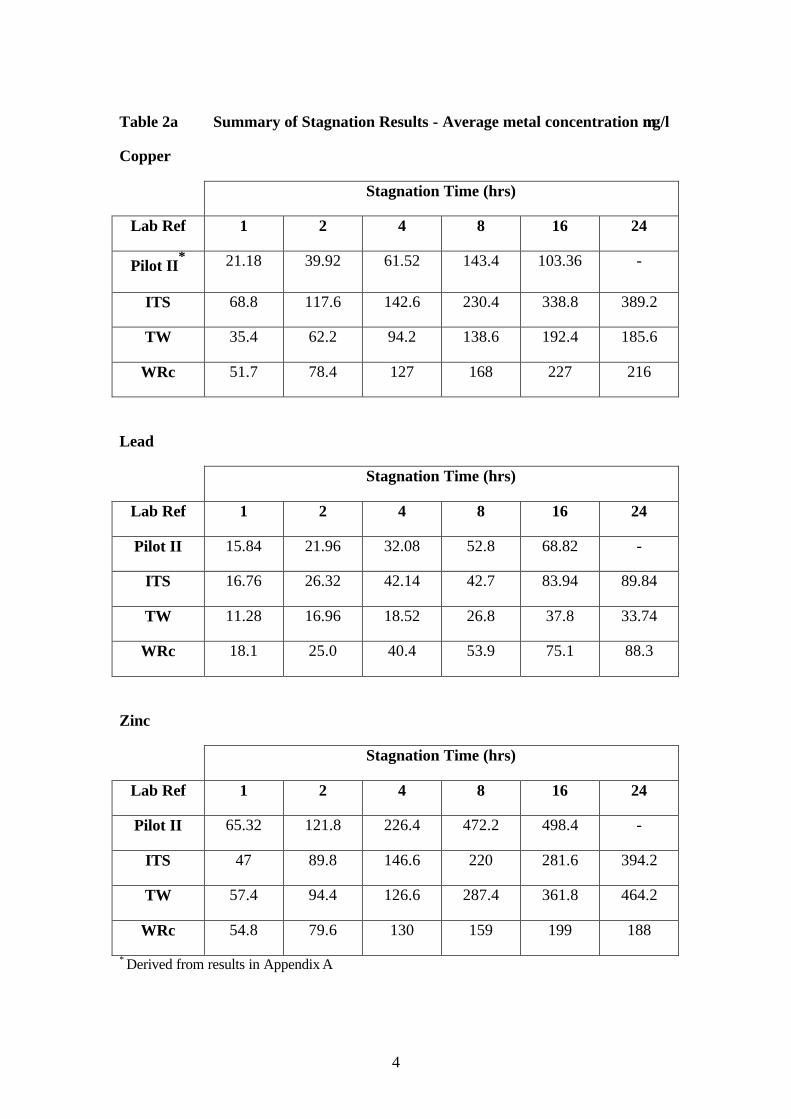
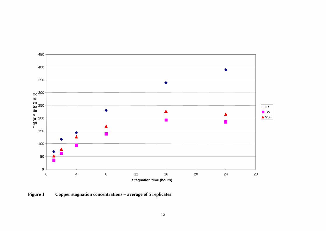
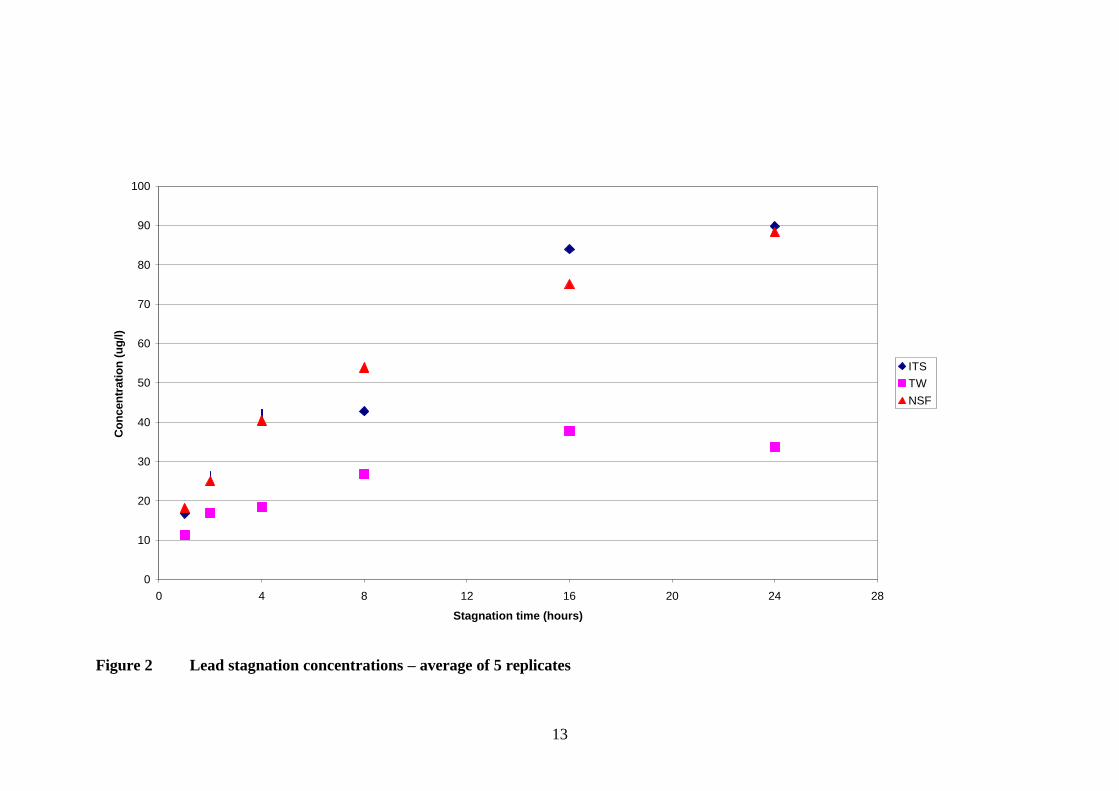
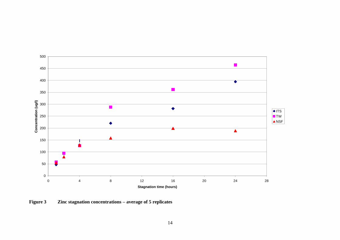
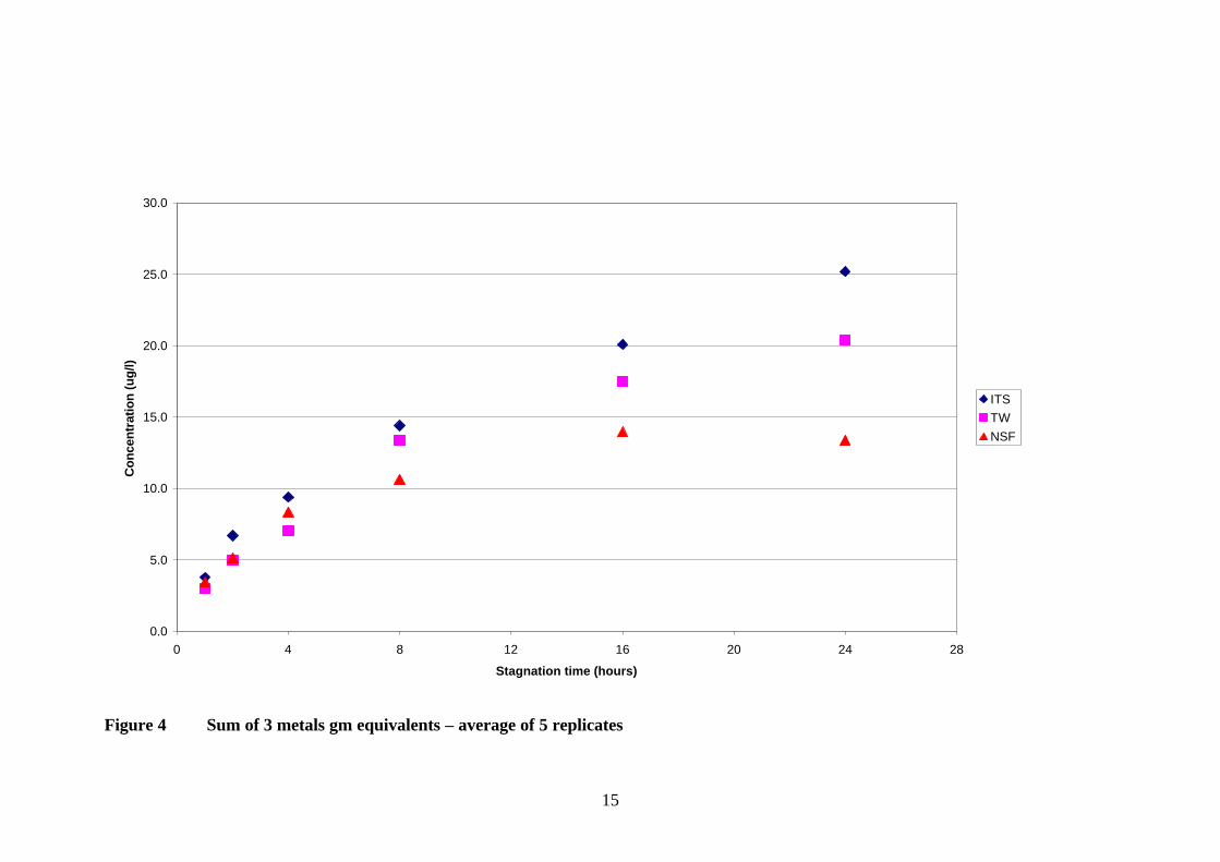
The results of this work are summarised in the Tables 1 and 2 below. The Pilot study results are averages of the data given in Appendix A (i.e. it has been assumed that depth of submersion of the coupons is indeed without effect). The increase in leachate concentration against stagnation time are presented in Figures 1, 2 and 3 for the individual elements analysed (Cu, Pb, Zn). Figure 4 shows the stagnation curve for all three metals combined as their micro-gram equivalents per litre.

Table 1 Test water analyses

Lab. Ref. Run Day

Ambient Temp oC

pH

Alkalinity mgCaCO3/l

Chloride mg/l

Sulphate mg/l

ITS 0 23 7.5 152 11 <10

TW 0 23.3 7.5 143 10 8.3

WRc 0 23.5 7.51 145 12.1 9.81

ITS Stag.1 23 7.5 154 11 <10

TW Stag.1 23.3 7.5 149 11 8.9

WRc Stag.1 23.5 7.54 157 16.5 9.23

Tolerances: 23 +/- 1 7.5 +/- 0.2 150 +/- 7.5 10 +/- 2 10 +/- 2

Note: Stag.1 = 1st of the stagnation days in which metal leachate samples were prepared.

4

Table 2a Summary of Stagnation Results - Average metal concentration µµg/l

Copper

Stagnation Time (hrs)

Lab Ref 1 2 4 8 16 24

Pilot II* 21.18 39.92 61.52 143.4 103.36 -

ITS 68.8 117.6 142.6 230.4 338.8 389.2

TW 35.4 62.2 94.2 138.6 192.4 185.6

WRc 51.7 78.4 127 168 227 216

Lead


Lab Ref 1 2 4 8 16 24

Pilot II 15.84 21.96 32.08 52.8 68.82 -

ITS 16.76 26.32 42.14 42.7 83.94 89.84

TW 11.28 16.96 18.52 26.8 37.8 33.74

WRc 18.1 25.0 40.4 53.9 75.1 88.3

Zinc


Lab Ref 1 2 4 8 16 24

Pilot II 65.32 121.8 226.4 472.2 498.4 -

ITS 47 89.8 146.6 220 281.6 394.2

TW 57.4 94.4 126.6 287.4 361.8 464.2

WRc 54.8 79.6 130 159 199 188

* Derived from results in Appendix A

5

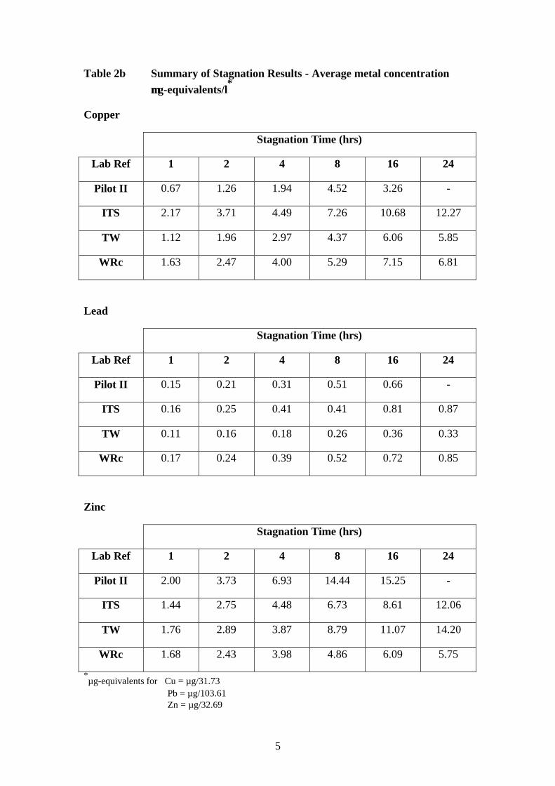
Table 2b Summary of Stagnation Results - Average metal concentration

µµg-equivalents/l*

Copper


Lab Ref 1 2 4 8 16 24

Pilot II 0.67 1.26 1.94 4.52 3.26 -

ITS 2.17 3.71 4.49 7.26 10.68 12.27

TW 1.12 1.96 2.97 4.37 6.06 5.85

WRc 1.63 2.47 4.00 5.29 7.15 6.81

Lead


Lab Ref 1 2 4 8 16 24

Pilot II 0.15 0.21 0.31 0.51 0.66 -

ITS 0.16 0.25 0.41 0.41 0.81 0.87

TW 0.11 0.16 0.18 0.26 0.36 0.33

WRc 0.17 0.24 0.39 0.52 0.72 0.85

Zinc


Lab Ref 1 2 4 8 16 24

Pilot II 2.00 3.73 6.93 14.44 15.25 -

ITS 1.44 2.75 4.48 6.73 8.61 12.06

TW 1.76 2.89 3.87 8.79 11.07 14.20

WRc 1.68 2.43 3.98 4.86 6.09 5.75

*µg-equivalents for Cu = µg/31.73

Pb = µg/103.61 Zn = µg/32.69

6

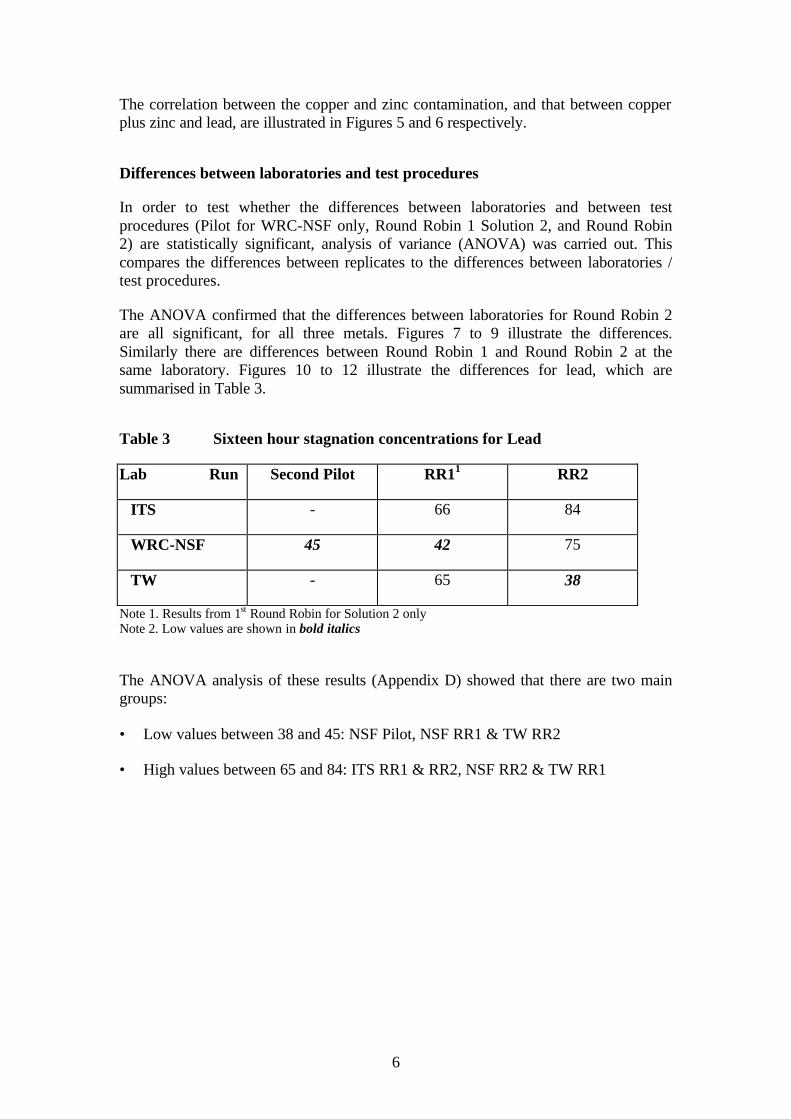
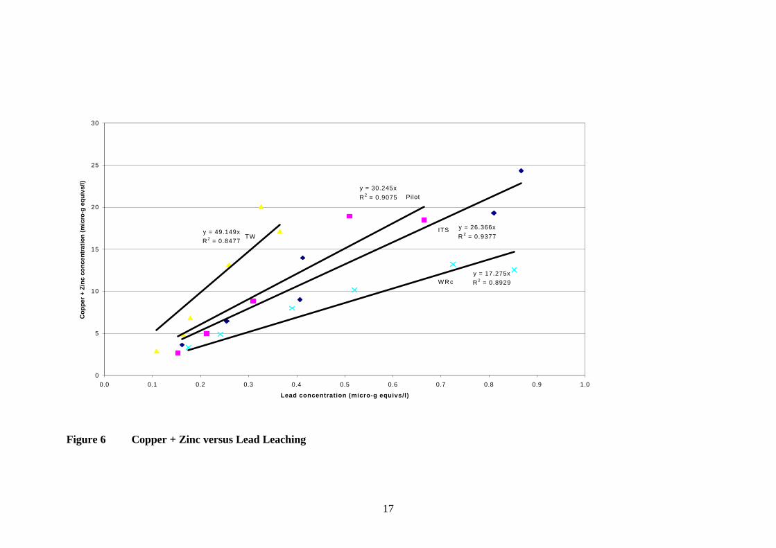
The correlation between the copper and zinc contamination, and that between copper plus zinc and lead, are illustrated in Figures 5 and 6 respectively.

Differences between laboratories and test procedures

In order to test whether the differences between laboratories and between test procedures (Pilot for WRC-NSF only, Round Robin 1 Solution 2, and Round Robin 2) are statistically significant, analysis of variance (ANOVA) was carried out. This compares the differences between replicates to the differences between laboratories / test procedures.

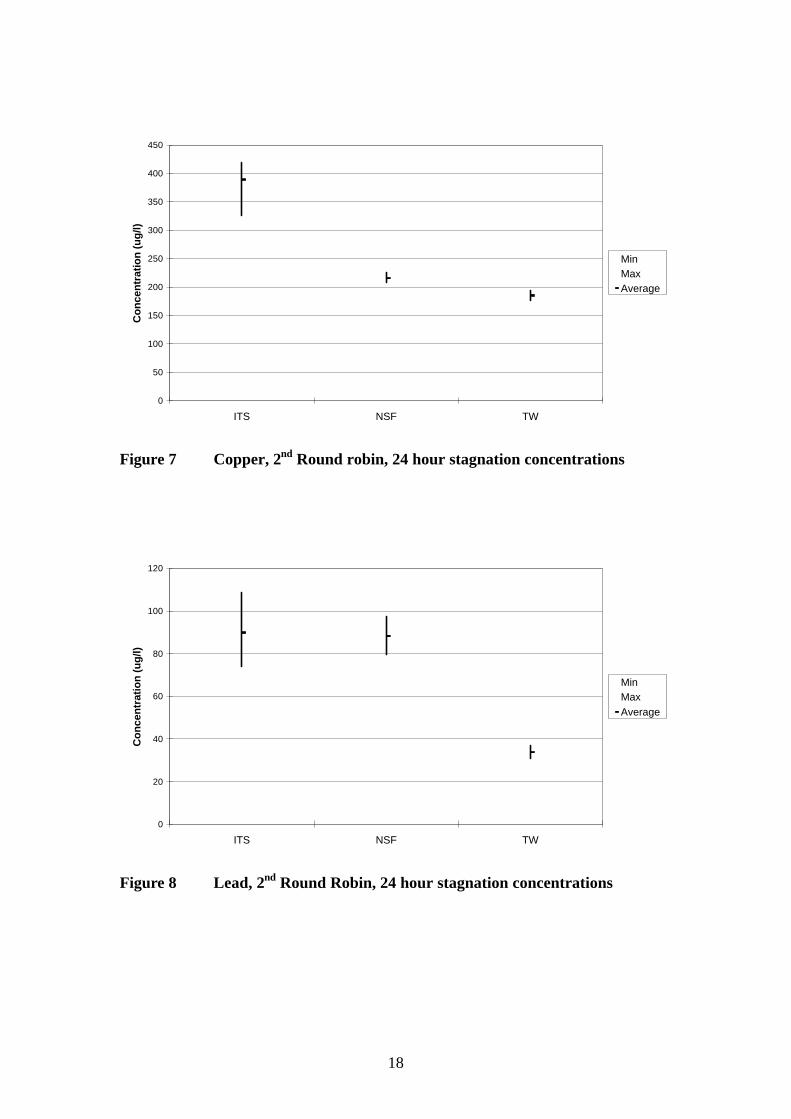
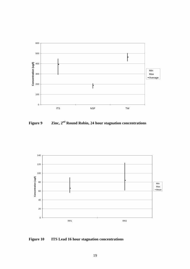
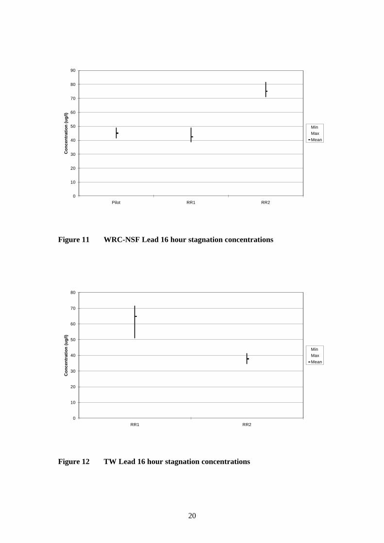
The ANOVA confirmed that the differences between laboratories for Round Robin 2 are all significant, for all three metals. Figures 7 to 9 illustrate the differences. Similarly there are differences between Round Robin 1 and Round Robin 2 at the same laboratory. Figures 10 to 12 illustrate the differences for lead, which are summarised in Table 3.

Table 3 Sixteen hour stagnation concentrations for Lead

Lab Run Second Pilot RR11 RR2

ITS - 66 84

WRC-NSF 45 42 75

TW - 65 38

Note 1. Results from 1st Round Robin for Solution 2 only Note 2. Low values are shown in bold italics

The ANOVA analysis of these results (Appendix D) showed that there are two main groups:

• Low values between 38 and 45: NSF Pilot, NSF RR1 & TW RR2

• High values between 65 and 84: ITS RR1 & RR2, NSF RR2 & TW RR1

7

3. DISCUSSION

It is immediately obvious from the Figures that the new test procedure has not improved the inter-laboratory reproducibility. It is apparent that, apart from the lead results from ITS and WRc-NSF laboratories and the combined metal curve from the Pilot and the ITS laboratory, the exponential stagnation curves for each metal are not tending to the same maximum, i.e. saturated solubility, value. This implies that the level of contamination cannot be under simple solubility control. As the study of the effects of depths of immersion of the test samples indicated that the contamination was not under simple corrosion control either, see Appendix A, this leaves us with some hybrid of the two mechanisms.

The 16-day ageing period of the test coupons used in the current test procedure is unlikely to ensure the full development of a corrosion product layer. This implies that the corrosion rate ought still to be a major factor in determining the contamination level in the water. Slight differences in the exposure conditions of the coupons could affect the physical form of the deposit produced during the ageing stage. These effects might continue to influence the service performance of the material in the long term because of the often critical nature of the initially formed film.

Interpretation of test results

In none of the tests of copper alloys, carried out in this or in any other similar programmes, has the leached levels for copper or zinc approached their PVC values, (2,000 and 5,000 µg/l respectively). Thus the decision as to the acceptability of these alloys from the point of view of these elements can be made unambiguously. This is not the case for lead. This is in a large measure due to the much lower PCV for lead (currently 50 µg/l) which would test the sensitivity of any procedure.

The current British Standard, DD 256:2002, recognises that amongst the possible outcomes of a test, as well as the usual pass or fail options, there can be a “null” result where the data does not allow a definitive decision to be made. The results of the present study can be used to define the limits of the null outcome for lead.

The lead results from all the tests carried out in this project are summarised in Table 4.

8

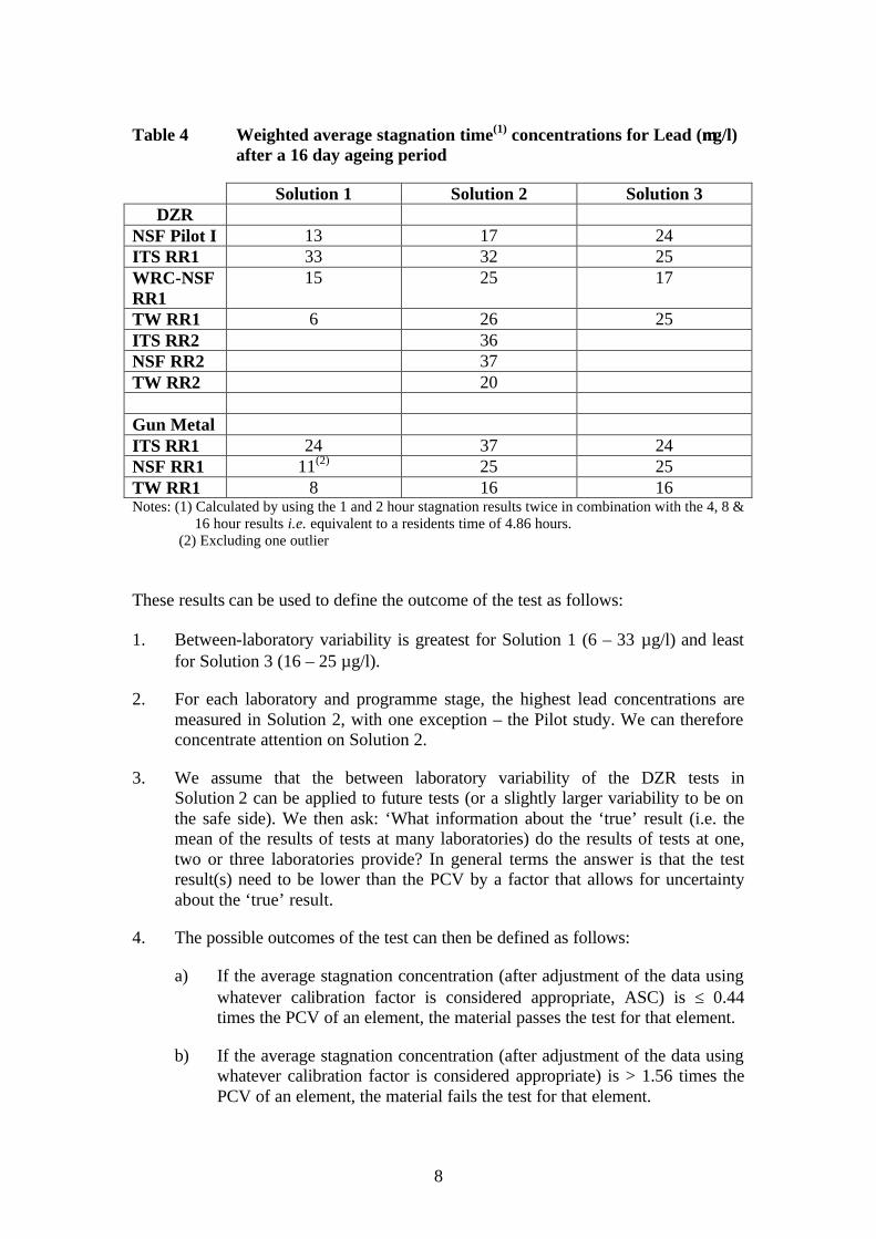
Table 4 Weighted average stagnation time(1) concentrations for Lead (µµg/l) after a 16 day ageing period

Solution 1 Solution 2 Solution 3 DZR

NSF Pilot I 13 17 24 ITS RR1 33 32 25 WRC-NSF RR1

15 25 17

TW RR1 6 26 25 ITS RR2 36 NSF RR2 37 TW RR2 20 Gun Metal ITS RR1 24 37 24 NSF RR1 11(2) 25 25 TW RR1 8 16 16 Notes: (1) Calculated by using the 1 and 2 hour stagnation results twice in combination with the 4, 8 &

16 hour results i.e. equivalent to a residents time of 4.86 hours. (2) Excluding one outlier These results can be used to define the outcome of the test as follows:

1. Between-laboratory variability is greatest for Solution 1 (6 – 33 µg/l) and least for Solution 3 (16 – 25 µg/l).

2. For each laboratory and programme stage, the highest lead concentrations are measured in Solution 2, with one exception – the Pilot study. We can therefore concentrate attention on Solution 2.

3. We assume that the between laboratory variability of the DZR tests in Solution 2 can be applied to future tests (or a slightly larger variability to be on the safe side). We then ask: ‘What information about the ‘true’ result (i.e. the mean of the results of tests at many laboratories) do the results of tests at one, two or three laboratories provide? In general terms the answer is that the test result(s) need to be lower than the PCV by a factor that allows for uncertainty about the ‘true’ result.

4. The possible outcomes of the test can then be defined as follows:

a) If the average stagnation concentration (after adjustment of the data using whatever calibration factor is considered appropriate, ASC) is ≤ 0.44 times the PCV of an element, the material passes the test for that element.

b) If the average stagnation concentration (after adjustment of the data using whatever calibration factor is considered appropriate) is > 1.56 times the PCV of an element, the material fails the test for that element.

9

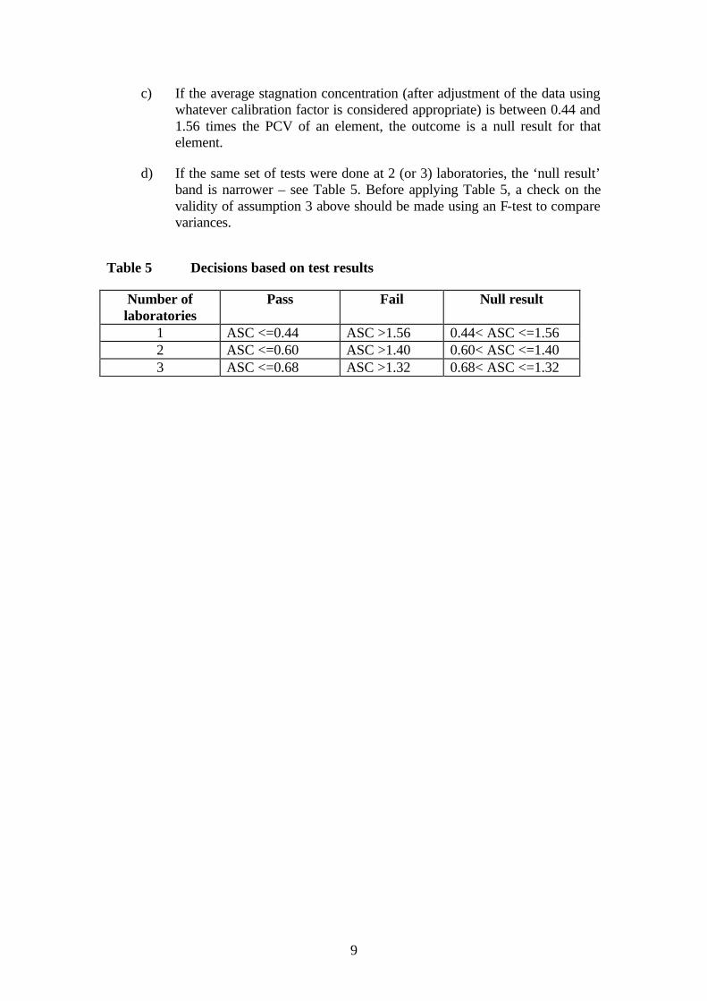
c) If the average stagnation concentration (after adjustment of the data using whatever calibration factor is considered appropriate) is between 0.44 and 1.56 times the PCV of an element, the outcome is a null result for that element.

d) If the same set of tests were done at 2 (or 3) laboratories, the ‘null result’ band is narrower – see Table 5. Before applying Table 5, a check on the validity of assumption 3 above should be made using an F-test to compare variances.

Table 5 Decisions based on test results

Number of laboratories

Pass Fail Null result

1 ASC <=0.44 ASC >1.56 0.44< ASC <=1.56 2 ASC <=0.60 ASC >1.40 0.60< ASC <=1.40 3 ASC <=0.68 ASC >1.32 0.68< ASC <=1.32

10

11

4. CONCLUSIONS

1. This work has developed a test procedure, based on plastic centrifuge tubes as the reaction vessels, that significantly increases the practical convenience and significantly reduces the cost of carrying out the testing of metals.

2. Strong correlations have been found between the concentrations of the major elements, i.e. copper, lead and zinc, that leach from the copper alloys. All show an exponential increase in concentration with time in the leachate water.

3. The amount of metal leached showed little sensitivity to the depth of immersion of the test coupon, suggesting little sensitivity to the level of dissolved oxygen in the test water. This in turn suggests that the contamination level achieved cannot be under the simple control of the alloy corrosion rate.

4. The exponential increases with time of a particular metal in the leachate water, found by the different test laboratories in most cases do not appear to be going to the same equilibrium value. This suggests that the contamination level achieved cannot be under the simple control of the solubility of the corrosion product formed.

5. The levels of copper and zinc leached in the tests were so far below their respective PCV’s that the acceptability for these elements of the alloys tested could be made unambiguously. This was not the case for lead.

6. Although the differences between measured lead concentrations at the three laboratories were considerable, a statistical procedure to decide the outcome of the test, that takes these ‘between laboratory’ differences into account, can be suggested.

12

Figure 1 Copper stagnation concentrations – average of 5 replicates

Figure 1: Copper stagnation concentrations - average of 5 replicates

0

50

100

150

200

250

300

350

400

450

0 4 8 12 16 20 24 28

Stagnation time (hours)

Concentration(ug/l)

ITS

TW

NSF

13

Figure 2 Lead stagnation concentrations – average of 5 replicates

Figure 2: Lead stagnation concentrations - average of 5 replicates

0

10

20

30

40

50

60

70

80

90

100

0 4 8 12 16 20 24 28


Co

nce

ntr

atio

n (

ug

/l)

ITS

TW

NSF

14

Figure 3 Zinc stagnation concentrations – average of 5 replicates

Figure 3: Zinc stagnation concentrations - average of 5 replicates

0

50

100

150

200

250

300

350

400

450

500

0 4 8 12 16 20 24 28


Co

nce

ntr

atio

n (

ug

/l)

ITS

TW

NSF

15

Figure 4 Sum of 3 metals gm equivalents – average of 5 replicates

Figure 4: Sum of 3 metals gm equivalents - average of 5 replicates

0.0

5.0

10.0

15.0

20.0

25.0

30.0

0 4 8 12 16 20 24 28


Co

nce

ntr

atio

n (

ug

/l)

ITS

TW

NSF

16

Figure 5. Correlations between Levels of Copper & Zinc Leaching

y = 0.9055x

R2 = 0.9632

y = 3.6491x

R 2 = 0.8892

y = 1.9977x

R 2 = 0.8971

y = 0.8855x

R 2 = 0.9704

0

2

4

6

8

10

12

14

16

18

0 2 4 6 8 10 12 14

Concentration of Copper (micro-g equivs/l)

Co

nce

ntr

atio

n o

f Z

inc

(mic

ro-g

eq

uiv

s/l)

ITS

Pilot

TW

WRc

Figure 5 Correlations between Levels of Copper and Zinc Leaching

17

Figure 6. Copper+Zinc versus Lead Leaching

y = 26.366x

R 2 = 0.9377

y = 30.245x

R2 = 0.9075

y = 49.149x

R2 = 0.8477

y = 17.275x

R2 = 0.8929

0

5

10

15

20

25

30

0.0 0.1 0.2 0.3 0.4 0.5 0.6 0.7 0.8 0.9 1.0

Lead concentration (micro-g equivs/l)

Co

pp

er +

Zin

c co

nce

ntr

atio

n (

mic

ro-g

eq

uiv

s/l)

ITS

Pilot

TW

WRc

Figure 6 Copper + Zinc versus Lead Leaching

18

Figure 7 Copper, 2nd Round robin, 24 hour stagnation concentrations

Figure 8 Lead, 2nd Round Robin, 24 hour stagnation concentrations

Figure 7: Copper, 2nd Round robin, 24 hour stagnation concentrations

0

50

100

150

200

250

300

350

400

450

ITS NSF TW

Co

nce

ntr

atio

n (

ug

/l)

Min Max Average

Figure 8: Lead, 2nd Round Robin, 24 hour stagnation concentrations

0

20

40

60

80

100

120

ITS NSF TW

Co

nce

ntr

atio

n (

ug

/l)

Min Max

Average

19

Figure 9 Zinc, 2nd Round Robin, 24 hour stagnation concentrations

Figure 10 ITS Lead 16 hour stagnation concentrations

Figure 9: Zinc,2nd Round Robin, 24 hour stagnation concentrations

0

100

200

300

400

500

600

ITS NSF TW

Co

nce

ntr

atio

n (

ug

/l)

Min Max Average

Figure 10: ITS Lead 16 hour stagnation concentrations

0

20

40

60

80

100

120

140

RR1 RR2

Co

nce

ntr

atio

n (

ug

/l)

Min

Max

Mean

20

Figure 11 WRC-NSF Lead 16 hour stagnation concentrations

Figure 12 TW Lead 16 hour stagnation concentrations

Figure 11: NSF Lead 16 hour stagnation concentrations

0

10

20

30

40

50

60

70

80

90

Pilot RR1 RR2

Co

nce

ntr

atio

n (

ug

/l)

Min

Max

Mean

Figure 12: TW Lead 16 hour stagnation concentrations

0

10

20

30

40

50

60

70

80

RR1 RR2

Co

nce

ntr

atio

n (

ug

/l)

Min

Max

Mean

21

APPENDIX A REPORT ON THE EFFECT OF DEPTH OF IMMERSION STUDY – SECOND PILOT USING MODIFIED DD 256:2002 PROCEDURE

Introduction

The results of the first Round Robin test showed a strong correlation between the combined level of copper and zinc leached into the test water with that of lead for both the CZ132 and LG4 alloys tested. For details see WRc-NSF report DWI 4079 July 2002. A possible explanation of this outcome could be that the phases of each alloy were competing for the same limited resource i.e. the dissolved oxygen in the test water. Slight differences in the depths of immersion of the test coupons might then explain the differences in the test results between laboratories. It was decided to test this hypothesis by exposing coupons at different depths in a test water thereby giving them different lengths to their respective diffusion paths to atmospheric oxygen.

Test method

Five replicate samples of the standard CZ132 coupons were exposed to 40 ml of Test Solution 2 (alkalinity 150 mg CaCO3/l, 10 mg/l of both chloride and sulphate) in capped plastic centrifuge tubes. As per the original method, the coupons were conditioned over 16 days using 24 hour stagnation periods. None of the leachate solutions were retained for metal analysis.

At the end of the 16 day conditioning period, the standard metal leaching vs. stagnation time procedure was carried out using stagnation periods of 1, 2, 4, 8 & 16 hours. The solutions obtained were analysed for Cu, Pb & Zn.

Results and Discussion

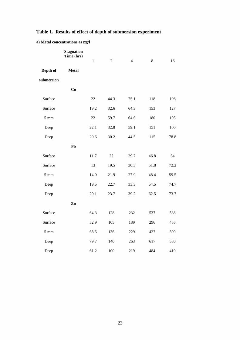
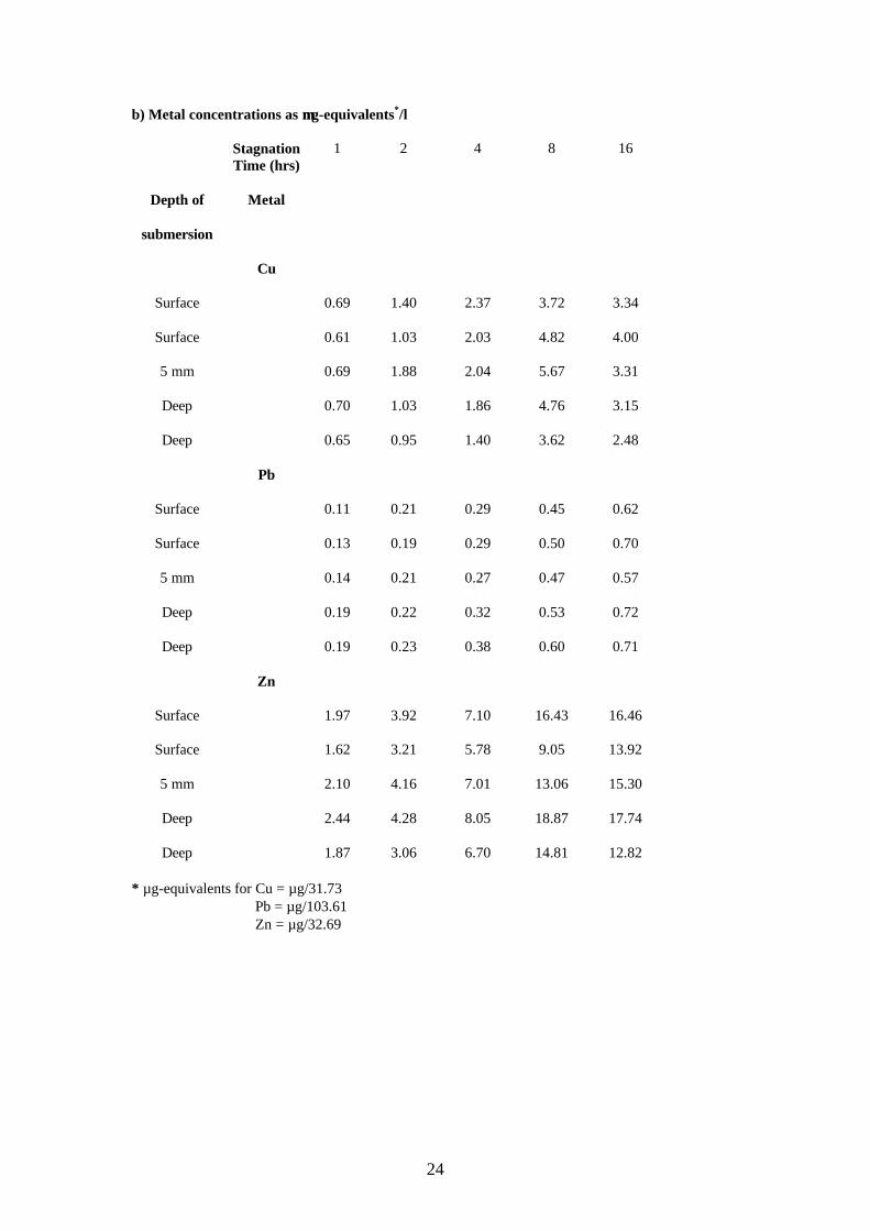
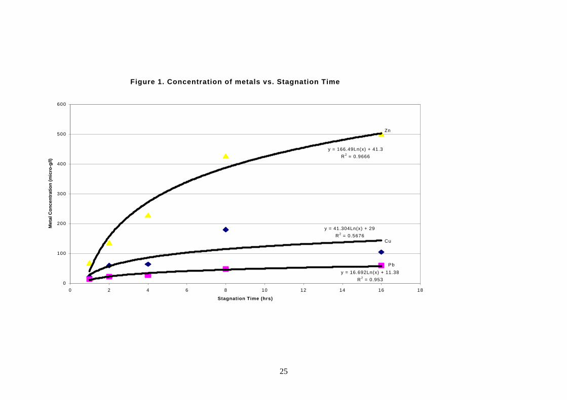
The results of this work, in units of µg/l and µg-equivalents/l, are given in the Tables 1a & 1b below. The increase in leachate concentration, for the individual elements analysed (Cu, Pb, Zn), against stagnation time is presented in Figure 1. These results show a better defined exponential pattern than that observed in the original Round Robin test. This may reflect the significantly higher surface area of coupon to test water volume in the modified procedure used in this work. If thought desirable, the ratio could be restored to the value specified in DD 256:2002 by reducing the coupon length when using test-tubes as the reaction containers.

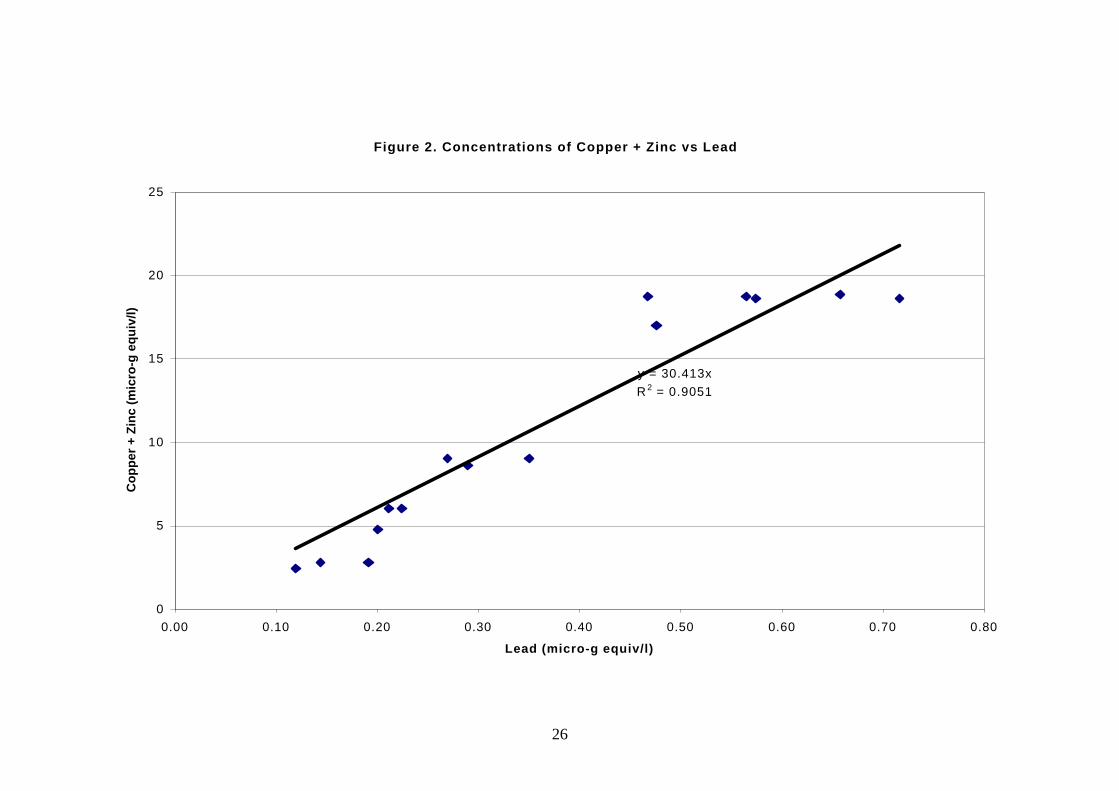
The relationship between the concentration of copper plus zinc leached with that for lead found in the Round Robin was observed even more strongly in this work; see Figure 2. However, it is quite clear from the results that the depth of immersion of the coupon is having little influence of the level of metal leached, see Table 1a. This means the relationship observed cannot arise, as originally thought, by the different phases of the alloy competing for the diffusion limited supply of dissolved oxygen.

22

This leaves a correlation in the rates of dissolution of the respective corrosion products formed by the elements concerned the exact value of which is determined by the ratio of the surface areas of the different phases in the alloy. This idea is supported by the fact that the correlation becomes less convincing at high concentrations of the elements (see Figure 2) when the rates of dissolution will significantly reduce as equilibrium solubility levels are approached.

Conclusions

� It is clear from the results of this work that the depth of immersion of the test coupons does not affect the leaching of metals in the test procedure followed.

� This means that the level contamination is not being controlled by the local concentration of dissolved oxygen, and hence the rates of corrosion achieved, which leaves the rate of dissolution of the corrosion products formed as the controlling mechanism.

RJO 16.9.02.

23

Table 1. Results of effect of depth of submersion experiment

a) Metal concentrations as µµg/l


1

2

4

8

16

Depth of Metal

submersion

Cu

Surface 22 44.3 75.1 118 106

Surface 19.2 32.6 64.3 153 127

5 mm 22 59.7 64.6 180 105

Deep 22.1 32.8 59.1 151 100

Deep 20.6 30.2 44.5 115 78.8

Pb

Surface 11.7 22 29.7 46.8 64

Surface 13 19.5 30.3 51.8 72.2

5 mm 14.9 21.9 27.9 48.4 59.5

Deep 19.5 22.7 33.3 54.5 74.7

Deep 20.1 23.7 39.2 62.5 73.7

Zn

Surface 64.3 128 232 537 538

Surface 52.9 105 189 296 455

5 mm 68.5 136 229 427 500

Deep 79.7 140 263 617 580

Deep 61.2 100 219 484 419

24

b) Metal concentrations as µµg-equivalents*/l


1 2 4 8 16

Depth of Metal

submersion

Cu

Surface 0.69 1.40 2.37 3.72 3.34

Surface 0.61 1.03 2.03 4.82 4.00

5 mm 0.69 1.88 2.04 5.67 3.31

Deep 0.70 1.03 1.86 4.76 3.15

Deep 0.65 0.95 1.40 3.62 2.48

Pb

Surface 0.11 0.21 0.29 0.45 0.62

Surface 0.13 0.19 0.29 0.50 0.70

5 mm 0.14 0.21 0.27 0.47 0.57

Deep 0.19 0.22 0.32 0.53 0.72

Deep 0.19 0.23 0.38 0.60 0.71

Zn

Surface 1.97 3.92 7.10 16.43 16.46

Surface 1.62 3.21 5.78 9.05 13.92

5 mm 2.10 4.16 7.01 13.06 15.30

Deep 2.44 4.28 8.05 18.87 17.74

Deep 1.87 3.06 6.70 14.81 12.82

* µg-equivalents for Cu = µg/31.73 Pb = µg/103.61 Zn = µg/32.69

25

Figure 1. Concentration of metals vs. Stagnation Time

y = 166.49Ln(x) + 41.3

R2 = 0.9666

y = 41.304Ln(x) + 29

R2 = 0.5676

y = 16.692Ln(x) + 11.38

R2 = 0.9530

100

200

300

400

500

600

0 2 4 6 8 10 12 14 16 18


Met

al C

on

cen

trat

ion

(m

icro

-g/l)

Zn

Cu

Pb

26

Figure 2. Concentrations of Copper + Zinc vs Lead

y = 30.413x

R 2 = 0.9051

0

5

10

15

20

25

0.00 0.10 0.20 0.30 0.40 0.50 0.60 0.70 0.80

Lead (micro-g equiv/l)

Co

pp

er +

Zin

c (m

icro

-g e

qu

iv/l)

27

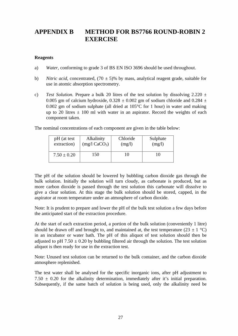
APPENDIX B METHOD FOR BS7766 ROUND-ROBIN 2 EXERCISE

Reagents

a) Water, conforming to grade 3 of BS EN ISO 3696 should be used throughout.

b) Nitric acid, concentrated, (70 ± 5)% by mass, analytical reagent grade, suitable for use in atomic absorption spectrometry.

c) Test Solution. Prepare a bulk 20 litres of the test solution by dissolving 2.220 ± 0.005 gm of calcium hydroxide, 0.328 ± 0.002 gm of sodium chloride and 0.284 ± 0.002 gm of sodium sulphate (all dried at 105°C for 1 hour) in water and making up to 20 litres ± 100 ml with water in an aspirator. Record the weights of each component taken.

The nominal concentrations of each component are given in the table below:

pH (at test extraction)

Alkalinity (mg/l CaCO3)

Chloride (mg/l)

Sulphate (mg/l)

7.50 ± 0.20 150 10 10

The pH of the solution should be lowered by bubbling carbon dioxide gas through the bulk solution. Initially the solution will turn cloudy, as carbonate is produced, but as more carbon dioxide is passed through the test solution this carbonate will dissolve to give a clear solution. At this stage the bulk solution should be stored, capped, in the aspirator at room temperature under an atmosphere of carbon dioxide.

Note: It is prudent to prepare and lower the pH of the bulk test solution a few days before the anticipated start of the extraction procedure.

At the start of each extraction period, a portion of the bulk solution (conveniently 1 litre) should be drawn off and brought to, and maintained at, the test temperature (23 ± 1 °C) in an incubator or water bath. The pH of this aliquot of test solution should then be adjusted to pH 7.50 ± 0.20 by bubbling filtered air through the solution. The test solution aliquot is then ready for use in the extraction test.

Note: Unused test solution can be returned to the bulk container, and the carbon dioxide atmosphere replenished.

The test water shall be analysed for the specific inorganic ions, after pH adjustment to 7.50 ± 0.20 for the alkalinity determination, immediately after it’s initial preparation. Subsequently, if the same batch of solution is being used, only the alkalinity need be

28

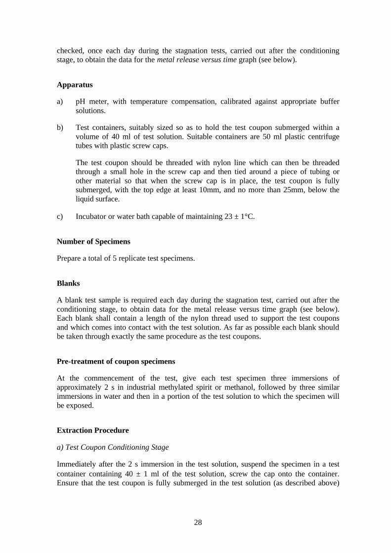
checked, once each day during the stagnation tests, carried out after the conditioning stage, to obtain the data for the metal release versus time graph (see below).

Apparatus

a) pH meter, with temperature compensation, calibrated against appropriate buffer solutions.

b) Test containers, suitably sized so as to hold the test coupon submerged within a volume of 40 ml of test solution. Suitable containers are 50 ml plastic centrifuge tubes with plastic screw caps.

The test coupon should be threaded with nylon line which can then be threaded through a small hole in the screw cap and then tied around a piece of tubing or other material so that when the screw cap is in place, the test coupon is fully submerged, with the top edge at least 10mm, and no more than 25mm, below the liquid surface.

c) Incubator or water bath capable of maintaining 23 ± 1°C.

Number of Specimens

Prepare a total of 5 replicate test specimens.

Blanks

A blank test sample is required each day during the stagnation test, carried out after the conditioning stage, to obtain data for the metal release versus time graph (see below). Each blank shall contain a length of the nylon thread used to support the test coupons and which comes into contact with the test solution. As far as possible each blank should be taken through exactly the same procedure as the test coupons.

Pre-treatment of coupon specimens

At the commencement of the test, give each test specimen three immersions of approximately 2 s in industrial methylated spirit or methanol, followed by three similar immersions in water and then in a portion of the test solution to which the specimen will be exposed.

Extraction Procedure

a) Test Coupon Conditioning Stage

Immediately after the 2 s immersion in the test solution, suspend the specimen in a test container containing 40 ± 1 ml of the test solution, screw the cap onto the container. Ensure that the test coupon is fully submerged in the test solution (as described above)

29

and that it is not touching the wall of the test container. Store in an incubator or water bath for 24 hr as the first 24 hr extraction period.

Following each extraction period lift the cap and test specimen gently clear of the surface of the test solution and allow it to drain for approximately 2 s before touching its lower edge momentarily on the liquid surface. Then re-immerse it and repeat the procedure twice. Transfer the test specimen immediately to another test container containing a fresh 40 ± 1 ml portion of test solution (brought to the correct temperature and pH as described above).

Discard the old test extract.

Repeat the extraction procedure for a minimum of a further 15 days.

b) Metal Release vs Time

At the end of the 16 day coupon-conditioning series of 24 hr extractions, a second stage of extractions is carried out.

The data required shall be obtained by consecutively exposing each test specimen to different samples of the test water for different periods and determining the concentration of metals in these extracts.

For the sake of reproducibility, and to avoid the necessity of overnight working, the stagnation times to be used, and their order of application, shall be 4, 2, 1, 0.5 hours (during day 1), 16 hours (overnight following), 8 hours (during the next day) and 24 hours.

Note that, due to reasons of practicability, there can be a delay between the completion of the 16 day conditioning period and the time when the stagnation procedure can be started. During this delay, the 24h extract test should be continued, so that the test materials are maintained under the original test conditions.

Suspend the specimen in a test container containing 40 ± 1 ml of the test solution, screw the cap onto the container. Ensure that the test coupon is fully submerged in the test solution (as described above) and that it is not touching the wall of the test container. Store at (23 ± 1) ºC in an incubator or water bath for the first stagnation period.

Following each stagnation period, lift the cap and test specimen gently clear of the surface of the test solution and allow it to drain for approximately 2 s before touching its lower edge momentarily on the liquid surface. Then re-immerse it and repeat the procedure twice. Transfer the test specimen immediately to another test container containing a fresh 40 ± 1 ml portion of test solution (brought to the correct temperature and pH as described above).

The container with the stagnation period test extract should then be acidified by adding 0.40 ± 0.05 ml of concentrated nitric acid. Cap the container with a new cap, mix the contents and leave to stand for a minimum of 12 hours before analysis for Copper, Zinc and Lead.

30

Repeat the extraction procedure for the remainder of the stagnation periods.

31

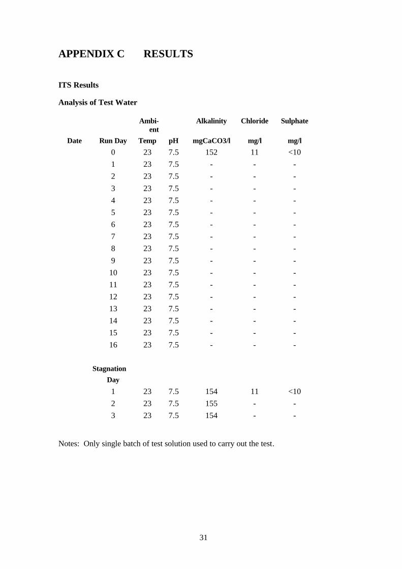
APPENDIX C RESULTS

ITS Results

Analysis of Test Water

Ambi-ent

Alkalinity Chloride Sulphate

Date Run Day Temp pH mgCaCO3/l mg/l mg/l

0 23 7.5 152 11 <10

1 23 7.5 - - -

2 23 7.5 - - -

3 23 7.5 - - -

4 23 7.5 - - -

5 23 7.5 - - -

6 23 7.5 - - -

7 23 7.5 - - -

8 23 7.5 - - -

9 23 7.5 - - -

10 23 7.5 - - -

11 23 7.5 - - -

12 23 7.5 - - -

13 23 7.5 - - -

14 23 7.5 - - -

15 23 7.5 - - -

16 23 7.5 - - -

Stagnation

Day

1 23 7.5 154 11 <10

2 23 7.5 155 - -

3 23 7.5 154 - -

Notes: Only single batch of test solution used to carry out the test.

32

ITS Results continued

Leachate Concentration vs Stagnation Time - DZR Brass Coupons

Time (Hrs)

Time (Hrs)

1.0 2.0 Cu Pb Zn Cu Pb Zn ug/l ug/l ug/l ug/l ug/l ug/l

Replicate 1 65 18.5 57 114 31.3 96 Replicate 2 73 16.2 45 113 25.80 89 Replicate 3 74 21.2 39 118 30.1 76 Replicate 4 72 16.2 42 130 27.5 84 Replicate 5 60 11.7 52 113 16.9 104

Average 68.8 16.76 47 117.6 26.32 89.8 Time

(Hrs) Time

(Hrs)

4 8 Replicate 1 138 45.7 131 220.0 43.9 217 Replicate 2 133 40 147 236 40.3 242 Replicate 3 141 52.8 129 230 50.9 193 Replicate 4 147 42.3 141 233 40.8 207 Replicate 5 154 29.9 185 233 37.8 241

Average 142.6 42.14 146.6 230.4 42.74 220 Time

(Hrs) Time

(Hrs)

16 24 Replicate 1 341 84.7 289 389 94.5 426 Replicate 2 409 79.3 350 420 87.3 448 Replicate 3 335 122.9 263 412 109.0 415 Replicate 4 314 71.3 258 398 84.5 389 Replicate 5 295 61.5 248 327 73.9 293

Average 338.8 83.94 281.6 389.2 89.84 394.2

Day 1 Blank <4 <0.5 10 Day 2 Blank 9 <0.5 <4 Day 3 Blank <4 <0.5 9

33

Thames Results

Analyses of the Test Water

Ambient Alkalinity Chloride Sulphate

Date Run Day Temp pH mgCaCO3/l mg/l mg/l

20/10/02 0 23.3 7.5 143 10 8.3

21/10/02 1 23.3 7.5 - - -

22/10/02 2 23.3 7.5 - - -

23/10/02 3 23.3 7.5 - - -

24/10/02 4 23.4 7.5 - - -

25/10/02 5 23.3 7.5 - - -

26/10/02 6 23.3 7.5 - - -

27/10/02 7 23.3 7.5 - - -

28/10/02 8 23.3 7.5 - - -

29/10/02 9 23.3 7.5 - - -

30/10/02 10 23.3 7.5 - - -

31/10/02 11 23.3 7.5 - - -

01/11/02 12 23.3 7.5 - - -

02/11/02 13 23.3 7.5 - - -

03/11/02 14 23.3 7.5 - - -

04/11/02 15 23.3 7.5 - - -

05/11/02 16 23.3 7.5 - - -

Stagnation

Day

06/11/02 1 23.3 7.5 149 11 8.9

07/11/02 2 23.3 7.5 149 - -

08/11/02 3 23.3 - - - -

Note: Only a single batch of test solution used to carry out the test.

34

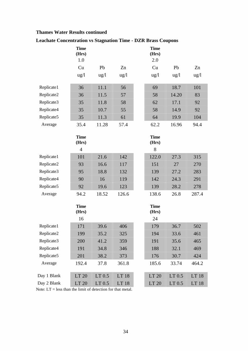
Thames Water Results continued


Time (Hrs)

Time (Hrs)


Replicate1 36 11.1 56 69 18.7 101 Replicate2 36 11.5 57 58 14.20 83 Replicate3 35 11.8 58 62 17.1 92 Replicate4 35 10.7 55 58 14.9 92 Replicate5 35 11.3 61 64 19.9 104 Average 35.4 11.28 57.4 62.2 16.96 94.4

Time (Hrs)

Time (Hrs)

4 8 Replicate1 101 21.6 142 122.0 27.3 315 Replicate2 93 16.6 117 151 27 270 Replicate3 95 18.8 132 139 27.2 283 Replicate4 90 16 119 142 24.3 291 Replicate5 92 19.6 123 139 28.2 278 Average 94.2 18.52 126.6 138.6 26.8 287.4

Time (Hrs)

Time (Hrs)

16 24 Replicate1 171 39.6 406 179 36.7 502 Replicate2 199 35.2 325 194 33.6 461 Replicate3 200 41.2 359 191 35.6 465 Replicate4 191 34.8 346 188 32.1 469 Replicate5 201 38.2 373 176 30.7 424 Average 192.4 37.8 361.8 185.6 33.74 464.2

Day 1 Blank LT 20 LT 0.5 LT 18 LT 20 LT 0.5 LT 18 Day 2 Blank LT 20 LT 0.5 LT 18 LT 20 LT 0.5 LT 18

Note: LT = less than the limit of detection for that metal.

35

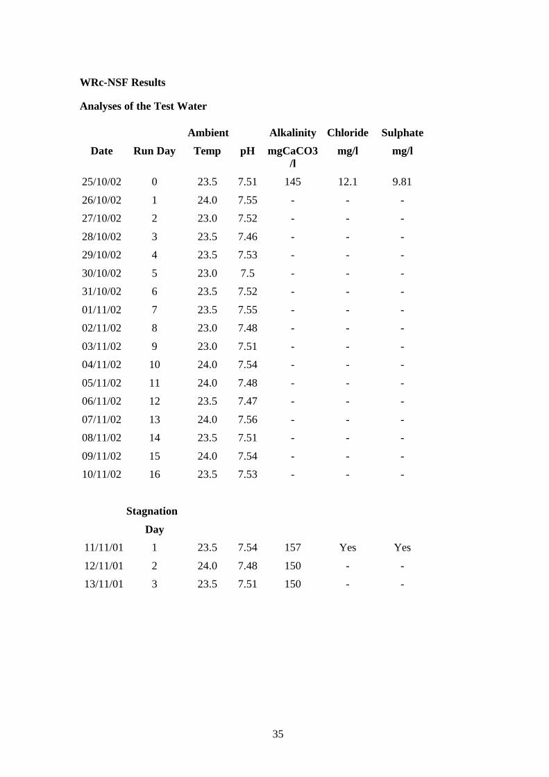
WRc-NSF Results

Analyses of the Test Water

Ambient Alkalinity Chloride Sulphate

Date Run Day Temp pH mgCaCO3/l

mg/l mg/l

25/10/02 0 23.5 7.51 145 12.1 9.81

26/10/02 1 24.0 7.55 - - -

27/10/02 2 23.0 7.52 - - -

28/10/02 3 23.5 7.46 - - -

29/10/02 4 23.5 7.53 - - -

30/10/02 5 23.0 7.5 - - -

31/10/02 6 23.5 7.52 - - -

01/11/02 7 23.5 7.55 - - -

02/11/02 8 23.0 7.48 - - -

03/11/02 9 23.0 7.51 - - -

04/11/02 10 24.0 7.54 - - -

05/11/02 11 24.0 7.48 - - -

06/11/02 12 23.5 7.47 - - -

07/11/02 13 24.0 7.56 - - -

08/11/02 14 23.5 7.51 - - -

09/11/02 15 24.0 7.54 - - -

10/11/02 16 23.5 7.53 - - -

Stagnation

Day

11/11/01 1 23.5 7.54 157 Yes Yes

12/11/01 2 24.0 7.48 150 - -

13/11/01 3 23.5 7.51 150 - -

36

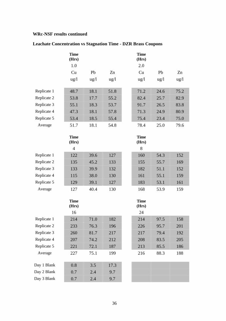
WRc-NSF results continued


Time (Hrs)

Time (Hrs)


Replicate 1 48.7 18.1 51.8 71.2 24.6 75.2 Replicate 2 53.8 17.7 55.2 82.4 25.7 82.9 Replicate 3 55.1 18.3 53.7 91.7 26.5 83.8 Replicate 4 47.3 18.1 57.8 71.3 24.9 80.9 Replicate 5 53.4 18.5 55.4 75.4 23.4 75.0

Average 51.7 18.1 54.8 78.4 25.0 79.6 Time

(Hrs) Time

(Hrs)


Average 127 40.4 130 168 53.9 159 Time

(Hrs) Time

(Hrs)


Average 227 75.1 199 216 88.3 188

Day 1 Blank 0.8 3.5 17.3 Day 2 Blank 0.7 2.4 9.7 Day 3 Blank 0.7 2.4 9.7

37

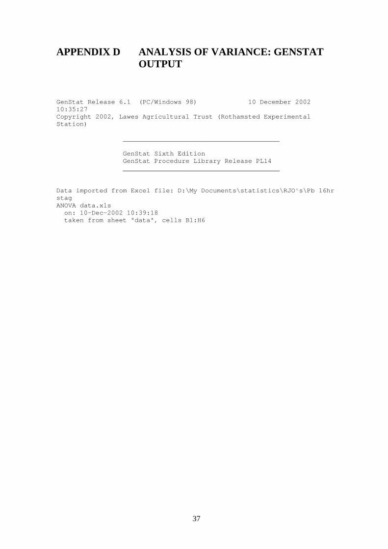
APPENDIX D ANALYSIS OF VARIANCE: GENSTAT OUTPUT

GenStat Release 6.1 (PC/Windows 98) 10 December 2002 10:35:27 Copyright 2002, Lawes Agricultural Trust (Rothamsted Experimental Station) ________________________________________ GenStat Sixth Edition GenStat Procedure Library Release PL14 ________________________________________ Data imported from Excel file: D:\My Documents\statistics\RJO's\Pb 16hr stag ANOVA data.xls on: 10-Dec-2002 10:39:18 taken from sheet "data", cells B1:H6

38

Summary statistics

Summary statistics for ITS_RR1 Number of values = 5 Mean = 66.20 Minimum = 56.00 Maximum = 90.00 Variance = 185.20 Summary statistics for ITS_RR2 Number of values = 5 Mean = 83.9 Minimum = 61.5 Maximum = 122.9 Variance = 550.8 Summary statistics for NSF_Pilot Number of values = 5 Mean = 45.10 Minimum = 41.40 Maximum = 48.70 Variance = 7.17 Summary statistics for NSF_RR1 Number of values = 5 Mean = 42.44 Minimum = 38.60 Maximum = 48.80 Variance = 19.01 Summary statistics for NSF_RR2 Number of values = 5 Mean = 75.06 Minimum = 71.00 Maximum = 81.70 Variance = 17.90 Summary statistics for TW_RR1 Number of values = 5 Mean = 64.78 Minimum = 51.01 Maximum = 71.41 Variance = 82.07 Summary statistics for TW_RR2 Number of values = 5 Mean = 37.80 Minimum = 34.80 Maximum = 41.20 Variance = 7.68

39

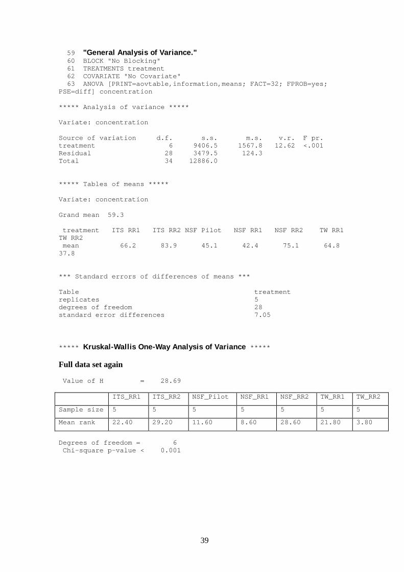
59 "General Analysis of Variance." 60 BLOCK "No Blocking" 61 TREATMENTS treatment 62 COVARIATE "No Covariate" 63 ANOVA [PRINT=aovtable,information,means; FACT=32; FPROB=yes; PSE=diff] concentration ***** Analysis of variance ***** Variate: concentration Source of variation d.f. s.s. m.s. v.r. F pr. treatment 6 9406.5 1567.8 12.62 <.001 Residual 28 3479.5 124.3 Total 34 12886.0 ***** Tables of means ***** Variate: concentration Grand mean 59.3 treatment ITS RR1 ITS RR2 NSF Pilot NSF RR1 NSF RR2 TW RR1 TW RR2 mean 66.2 83.9 45.1 42.4 75.1 64.8 37.8 *** Standard errors of differences of means *** Table treatment replicates 5 degrees of freedom 28 standard error differences 7.05

***** Kruskal-Wallis One-Way Analysis of Variance *****

Full data set again

Value of H = 28.69 ITS_RR1 ITS_RR2 NSF_Pilot NSF_RR1 NSF_RR2 TW_RR1 TW_RR2

Sample size 5 5 5 5 5 5 5

Mean rank 22.40 29.20 11.60 8.60 28.60 21.80 3.80

Degrees of freedom = 6 Chi-square p-value < 0.001

40

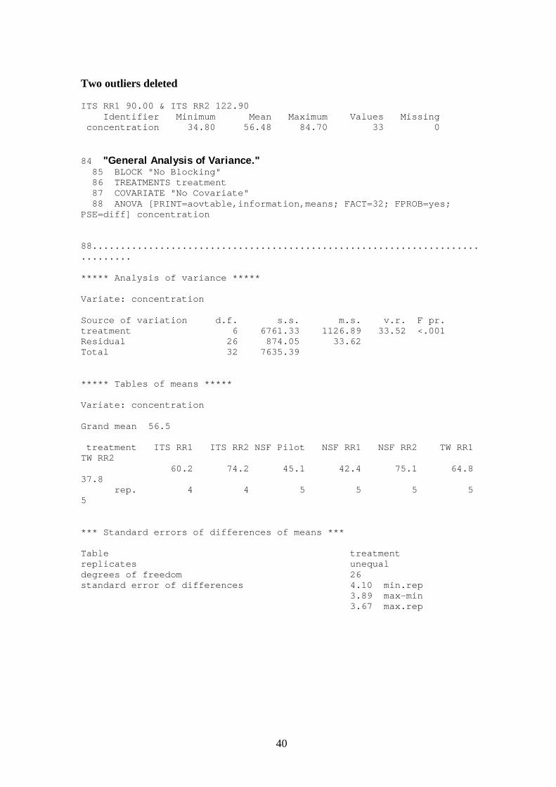
Two outliers deleted

ITS RR1 90.00 & ITS RR2 122.90 Identifier Minimum Mean Maximum Values Missing concentration 34.80 56.48 84.70 33 0

84 "General Analysis of Variance." 85 BLOCK "No Blocking" 86 TREATMENTS treatment 87 COVARIATE "No Covariate" 88 ANOVA [PRINT=aovtable,information,means; FACT=32; FPROB=yes; PSE=diff] concentration 88.............................................................................. ***** Analysis of variance ***** Variate: concentration Source of variation d.f. s.s. m.s. v.r. F pr. treatment 6 6761.33 1126.89 33.52 <.001 Residual 26 874.05 33.62 Total 32 7635.39 ***** Tables of means ***** Variate: concentration Grand mean 56.5 treatment ITS RR1 ITS RR2 NSF Pilot NSF RR1 NSF RR2 TW RR1 TW RR2 60.2 74.2 45.1 42.4 75.1 64.8 37.8 rep. 4 4 5 5 5 5 5 *** Standard errors of differences of means *** Table treatment replicates unequal degrees of freedom 26 standard error of differences 4.10 min.rep 3.89 max-min 3.67 max.rep

41

APPENDIX E DERIVATION OF TEST OUTCOME RULES

Key assumption

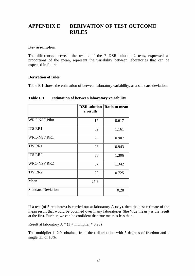
The differences between the results of the 7 DZR solution 2 tests, expressed as proportions of the mean, represent the variability between laboratories that can be expected in future.

Derivation of rules

Table E.1 shows the estimation of between laboratory variability, as a standard deviation.

Table E.1 Estimation of between laboratory variability

DZR solution 2 results

Ratio to mean

WRC-NSF Pilot 17 0.617

ITS RR1 32 1.161

WRC-NSF RR1 25 0.907

TW RR1 26 0.943

ITS RR2 36 1.306

WRC-NSF RR2 37 1.342

TW RR2 20 0.725

Mean 27.6

Standard Deviation 0.28

If a test (of 5 replicates) is carried out at laboratory A (say), then the best estimate of the mean result that would be obtained over many laboratories (the ‘true mean’) is the result at the first. Further, we can be confident that true mean is less than:

Result at laboratory A * (1 + multiplier * 0.28)

The multiplier is 2.0, obtained from the t distribution with 5 degrees of freedom and a single tail of 10%.

42

Similarly we can be confident that the true mean is greater than:

Result at laboratory A * (1 - multiplier * 0.28)

Similarly, if tests at N (= 2 or more) laboratories are carried out, the 80%ile range for the true mean is:

Mean of results at N laboratories * (1 +/- multiplier * 0.28 / �N )

The values for N = 1, 2 and 3 are shown in the main text, table 5.