Relocation of Eastern Tennessee Earthquakes Using

hypoDD

by

Meredith M. Dunn

Thesis submitted to the Faculty of the Virginia Polytechnic Institute and State University in partial

fulfillment of the requirements for the degree of

Masters of Science in Geophysics in the

Department of Geosciences

Martin C. Chapman, Chair John A. Hole

J. Arthur Snoke

August 2, 2004 Blacksburg, Virginia

(Keywords: Earthquakes, Eastern Tennessee Seismic Zone,

Hypocenter Relocation)

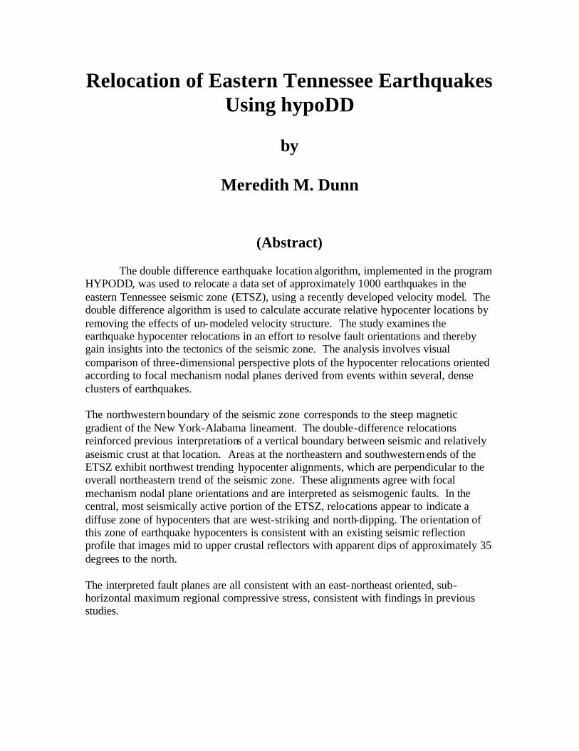
Relocation of Eastern Tennessee Earthquakes Using hypoDD

by

Meredith M. Dunn

(Abstract) The double difference earthquake location algorithm, implemented in the program HYPODD, was used to relocate a data set of approximately 1000 earthquakes in the eastern Tennessee seismic zone (ETSZ), using a recently developed velocity model. The double difference algorithm is used to calculate accurate relative hypocenter locations by removing the effects of un-modeled velocity structure. The study examines the earthquake hypocenter relocations in an effort to resolve fault orientations and thereby gain insights into the tectonics of the seismic zone. The analysis involves visual comparison of three-dimensional perspective plots of the hypocenter relocations oriented according to focal mechanism nodal planes derived from events within several, dense clusters of earthquakes. The northwestern boundary of the seismic zone corresponds to the steep magnetic gradient of the New York-Alabama lineament. The double-difference relocations reinforced previous interpretations of a vertical boundary between seismic and relatively aseismic crust at that location. Areas at the northeastern and southwestern ends of the ETSZ exhibit northwest trending hypocenter alignments, which are perpendicular to the overall northeastern trend of the seismic zone. These alignments agree with focal mechanism nodal plane orientations and are interpreted as seismogenic faults. In the central, most seismically active portion of the ETSZ, relocations appear to indicate a diffuse zone of hypocenters that are west-striking and north-dipping. The orientation of this zone of earthquake hypocenters is consistent with an existing seismic reflection profile that images mid to upper crustal reflectors with apparent dips of approximately 35 degrees to the north. The interpreted fault planes are all consistent with an east-northeast oriented, sub-horizontal maximum regional compressive stress, consistent with findings in previous studies.

iii

ACKNOWLEDGMENTS I would like to express my deepest gratitude to my advisor, Dr. Martin Chapman.

He suggested the topic of this thesis, provided unlimited instruction and guidance in my

studies, and provided me with the research assistantship that made it possible. I thank

him for his wisdom, patience, and continued support in my academic endeavors. I also

thank Dr. J.A. Snoke for his painstaking instruction in the classroom and his

contributions to the writing of the manuscript. Thanks to Dr. John Hole for his review

and comments on the manuscript.

Thanks go to the faculty and staff of Virginia Polytechnic Institute and State

University who have provided me the necessary atmosphere, instruction, and resources to

undertake this project. Also, a very special thanks to my fellow geophysics graduate

students, from whom I have learned so much and without whom I would not have been

able to complete this project or the necessary class work.

My sincerest gratitude goes to my family. My father and mother, Scott and Amy,

have seen me through all situations in my life to help me reach this place. Thanks to my

siblings, Marsha, Michael, and Mark for supporting me and helping me have fun along

the way. They continue to be an inspiration to my life.

The financial support for my graduate studies was provided through grant award

number 01HQAG0016 through the United States Geological Survey.

iv

Table of Contents Introduction…………………………………………………….………… 1

Chapter 1: Geologic and Tectonic History of the Study Area………… 4

Previous Studies of the Eastern Tennessee Seismic Zone………………………... 7

Summary…………………………………………………………………………….. 12

Chapter 2: Description and Analysis Approach………………….......... 14

Double-Difference Algorithm……………………………………...………..……... 15

HypoDD………………………………………………………………………...... …. 19

Example of hypoDD from Hayward Fault, California………………………........ 25

Chapter 3: Testing HypoDD with a Synthetic Data Set……………. ... 28

Chapter 4: HypoDD applied to the Eastern Tennessee Seismic Zone……………………………………………………………... 34

MAXSEP 20 km……………………………………………………………………... 35

MAXSEP 10 km…………………………………………………………………….. 37

Cluster 1, MAXSEP 10 km……………………………………………………..… 37

Cluster 2, MAXSEP 10 km…………………………………………………..…… 41

Cluster 3, MAXSEP 10 km…………………………………………………..…… 43

Cluster 4,5, and 6, MAXSEP 10 km........................................................................ 48

MAXSEP 5 km…………………………………………………………………...… 49

Cluster 1, MAXSEP 5 km…………………………………………………..…… 50

Cluster 2, MAXSEP 5 km………………………………………………..………. 52

Cluster 3, MAXSEP 5 km……………………………………………..…………. 56

v

Combined Subset of Clusters 1 and 2, MAXSEP 5 km……………......……….. 58

Sensitivity Testing of hypoDD…………………………………………………… 62

Conclusions…………………………………………………………..….. 64

References……………………………………………………………..…. 68

Appendix 1.………………………………………………………….…… 71

Appendix 2……………………………………………………………………………73

Appendix 3…………………………………………………………....………………74

vi

List of Illustrations Figure 1 The Eastern Tennessee Seismic Zone………………………………….……3

Figure 1.1 Magnetic Intensity and Bouguer Gravity Anomalies of NY-AL lineament..7

Figure 1.2 Focal Mechanisms for eastern Tennessee seismic zone…………………....12

Figure 2.1 Illustration of hypoDD parameters…………………………………………22

Figure 2.2 Example of hypoDD from Northern Hayward Fault…………………….…26

Figure 3.1 HYPOELLIPSE locations of synthetic data using error- free arrival times...28

Figure 3.2 HYPOELLIPSE locations of synthetic data using systematic errors………30

Figure 3.3 HYPODD relocations of synthetic data using systematic errors………...…31

Figure 3.4 HYPOELLIPSE locations of synthetic data containing systematic and

random errors………………………………………………………………32

Figure 3.5 HYPODD relocations of synthetic data containing systematic and random

errors……………………………………………………………………….33

Figure 4.1 MAXSEP 20 km…………………………………………………………....36

Figure 4.2 Cluster Locations, MAXSEP 10 km……….………………………...…….38

Figure 4.3 Cluster 1,MAXSEP 10 km-Comparison of Epicenters……….………...….39

Figure 4.4 Cluster 1, MAXSEP 10 km-Comparison of Hypocenters…………….……40

Figure 4.5 Cluster 2, MAXSEP 10 km…………………………………...……………44

Figure 4.6 Cluster 3, MAXSEP 10 km-Comparison of Epicenters………………...….45

Figure 4.7 Cluster 3, MAXSEP 10 km-Comparison of Hypocenters……………….....47

Figure 4.8 Cluster 4, MAXSEP 10 km………………………………...………………48

Figure 4.9 Cluster Locations, MAXSEP 5 km…………………………..…………….50

vii

Figure 4.10 Cluster 1, MAXSEP 5 km……………………………………..…………..53

Figure 4.11 Cluster 2, MAXSEP 5 km………………………………………...……….55

Figure 4.12 Cluster 3, MAXSEP 5 km…………………………………………..……..57

Figure 4.13 Subset of Clusters 1 and 2, MAXSEP 5 km……………………………….59

Figure 4.14 ARAL1 Reflection Profile………………………………………...……….61

Figure 4.15 Interpreted Orientations of Possible Seismogenic Features……….…….67

viii

List of Tables Table 4.1 Cluster Breakdown, MAXSEP 10 km………………………....……………41

Table 4.2 Focal Mechanisms Solutions…………………………………...…………..43

Table 4.3 Cluster Breakdown, MAXSEP 5 km………………………………………..49

1

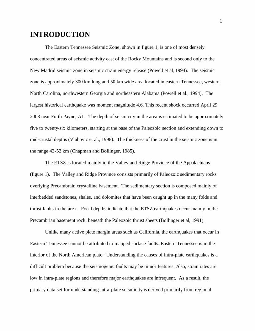
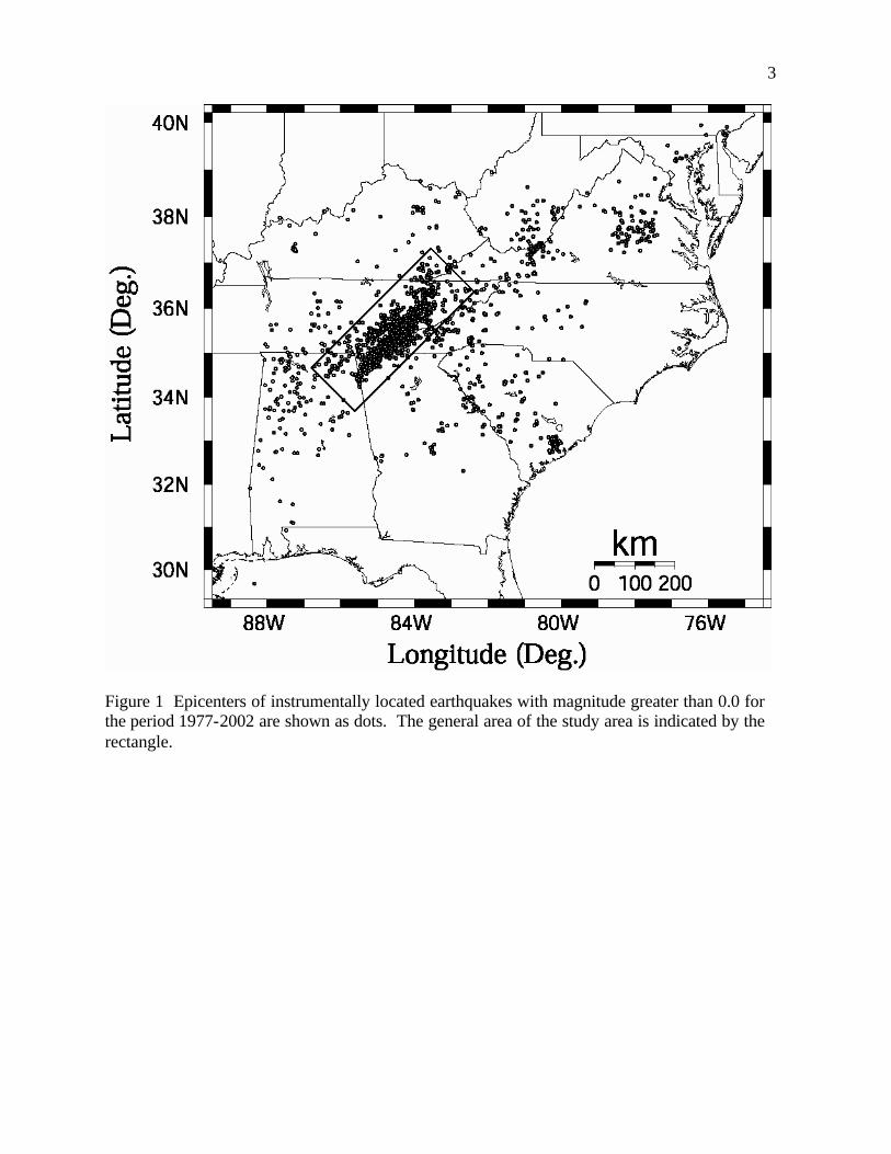
INTRODUCTION The Eastern Tennessee Seismic Zone, shown in figure 1, is one of most densely

concentrated areas of seismic activity east of the Rocky Mountains and is second only to the

New Madrid seismic zone in seismic strain energy release (Powell et al, 1994). The seismic

zone is approximately 300 km long and 50 km wide area located in eastern Tennessee, western

North Carolina, northwestern Georgia and northeastern Alabama (Powell et al., 1994). The

largest historical earthquake was moment magnitude 4.6. This recent shock occurred April 29,

2003 near Forth Payne, AL. The depth of seismicity in the area is estimated to be approximately

five to twenty-six kilometers, starting at the base of the Paleozoic section and extending down to

mid-crustal depths (Vlahovic et al., 1998). The thickness of the crust in the seismic zone is in

the range 43-52 km (Chapman and Bollinger, 1985).

The ETSZ is located mainly in the Valley and Ridge Province of the Appalachians

(figure 1). The Valley and Ridge Province consists primarily of Paleozoic sedimentary rocks

overlying Precambrain crystalline basement. The sedimentary section is composed mainly of

interbedded sandstones, shales, and dolomites that have been caught up in the many folds and

thrust faults in the area. Focal depths indicate that the ETSZ earthquakes occur mainly in the

Precambrian basement rock, beneath the Paleozoic thrust sheets (Bollinger et al, 1991).

Unlike many active plate margin areas such as California, the earthquakes that occur in

Eastern Tennessee cannot be attributed to mapped surface faults. Eastern Tennessee is in the

interior of the North American plate. Understanding the causes of intra-plate earthquakes is a

difficult problem because the seismogenic faults may be minor features. Also, strain rates are

low in intra-plate regions and therefore major earthquakes are infrequent. As a result, the

primary data set for understanding intra-plate seismicity is derived primarily from regional

2

network monitoring of small magnitude earthquakes. In the case of ETSZ, the seismicity occurs

in the Precambrian basement and may be totally unrelated to the surface geology. Knowledge

of the locations and orientations of brittle faults in the Precambrian Basement rocks of the ETSZ

is fundamental for understanding the nature of the seismicity. The faults may exist as a result of

the long and complex tectonic history of the Southern Appalachians. Modern seismicity may be

occurring on ancient faults that are being reactivated in the current stress field.

The purpose of my study is to examine the fault orientation in the Eastern Tennessee

Seismic Zone. I approach the problem by using an earthquake location algorithm developed by

Felix Waldhauser and William Ellsworth (2000). The program that implements the algorithm is

named HYPODD (Waldhauser, 2001).

HYPODD is based on a double difference approach that greatly reduces the errors in

relative earthquake locations introduced by un-modeled velocity variations. The algorithm

produces more reliable relative hypocenter locations than does the standard individual event

location approach (e.g., Hypoellipse, Lahr, 1980). A number of conditions must be fulfilled in

order for the potential advantages of the double difference algorithm to be realized. These

conditions, along with the theory underlying the double difference algorithm will be reviewed

below in chapter #2

Accurate relative hypocenter locations and earthquake focal mechanisms are most

important for understanding the tectonic framework of a seismically active area. Hypocenter

clusters in the seismic zone provide the only available data set from which the orientations of

potential seismogenic faults can be inferred. Therefore, the relocation of earthquake hypocenters

in the Eastern Tennessee Seismic Zone (ETSZ) is the basic objective of my study. Focal

mechanisms greatly aid in the interpretation of the results obtained from the relocation effort.

3

Figure 1 Epicenters of instrumentally located earthquakes with magnitude greater than 0.0 for the period 1977-2002 are shown as dots. The general area of the study area is indicated by the rectangle.

4

Chapter 1: Geologic and Tectonic History of the Study Area The geologic history of the study area is complex. Seismicity occurs within Precambrian

basement rocks that are covered by younger Paleozoic thrust sheets. The tectonic history of the

basement is most relevant to this study. The modern seismicity indicates that basement faults are

being reactivated by a modern stress field that may or may not be aligned with the ancient stress

field that originally created the basement tectonic fabric.

The first major tectonic event to impact the Southern Appalachian region was the

Grenville Orogeny approximately 1.3 to 1.1 billion years ago. Seismicity is occurring in

Grenville basement rocks. The Grenville orogeny was the culmination of the formation of the

supercontinent Rodinia. Between 600 and 800 million years ago, Rodinia fragmented and

subsequently re- formed as a new supercontinent, Pannotia. At the beginning of the Paleozoic,

Pannotia broke up yielding Laurentia (North America and Greenland) Gondwana (South

America, Africa, Antarctica, India, and Australia), Siberia and Baltica and creating the Iapetus

Ocean. As the Iapetus Ocean grew, a passive plate margin was formed along the eastern edge of

Laurentia, or proto- North America (Marshak, 2001).

The next major collisional orogenic event to affect the eastern margin of Laurentia was

the Taconic Orogeny, in the middle Ordovician, marking the collision of Laurentia with a

volcanic island arc. The collision deformed and metamorphosed strata of the former passive

margin basin and created a mountain range (Marshak, 2001). In the Devonian (380 million years

ago) another continent- island arc collision occurred, resulting in the Acadian Orogeny (Wheeler,

1995).

5

The final closing of the Iapetus Ocean occurred 250 to 300 million years ago, in the

Permian. This was a major continent-continent collision believed to be between the proto-North

American continent and the South American continent (Wheeler, 1995). The result of this

continent-continent collision was the formation of the supercontinent Pangea. The deformation

associated with the formation of Pangea is known in eastern North America as the Alleghanian

Orogeny and is the major episode of deformation in the southern Appalachian region (Cook et

al., 1979).

Pangea began to break apart in the Late Triassic. At the end of the Jurassic, rifting had

created the early Atlantic Ocean (Marshak, 2001). Eastern North America was in an extensional

stress field regime and rift basins developed along the Appalachian margin. The modern day

stress field has been in place since the Cretaceous, approximately 70 million years ago. This is a

compressive stress field, produced from an initial continental resistance to plate motion and from

ridge-push along the East Coast (Zoback & Zoback, 1991).

The eastern margin of North America was tectonically active during the Paleozoic and

early Mesozoic (Marshak, 2001). Since the Cretaceous, the area has been a passive margin.

There is no obvious explanation for many of the aspects of the seismicity of eastern North

America in the context of plate tectonics. Generally, it is accepted that the seismicity is due to

reactivation of existing faults (Wheeler, 1995 and references therein); however, the question

remains as to the location and type of the faults and when the faults were originally formed. For

example, one explanation for seismicity in the Valley and Ridge and Blue Ridge regions

proposed by Wheeler (1995) holds that the earthquakes occur as compressional reactivation of

normal faults formed originally during the rifting of Pannotia and opening of the Iapetus Ocean.

Other authors have proposed possible relationships between a variety of geological and

6

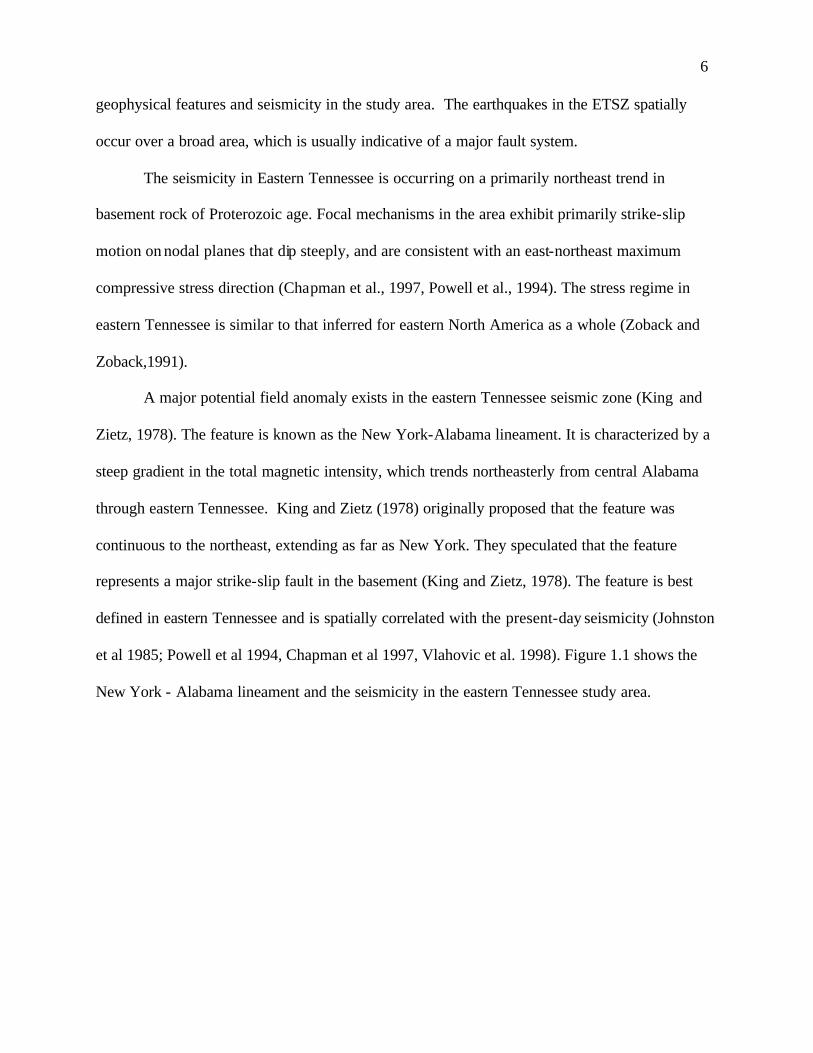
geophysical features and seismicity in the study area. The earthquakes in the ETSZ spatially

occur over a broad area, which is usually indicative of a major fault system.

The seismicity in Eastern Tennessee is occurring on a primarily northeast trend in

basement rock of Proterozoic age. Focal mechanisms in the area exhibit primarily strike-slip

motion on nodal planes that dip steeply, and are consistent with an east-northeast maximum

compressive stress direction (Chapman et al., 1997, Powell et al., 1994). The stress regime in

eastern Tennessee is similar to that inferred for eastern North America as a whole (Zoback and

Zoback,1991).

A major potential field anomaly exists in the eastern Tennessee seismic zone (King and

Zietz, 1978). The feature is known as the New York-Alabama lineament. It is characterized by a

steep gradient in the total magnetic intensity, which trends northeasterly from central Alabama

through eastern Tennessee. King and Zietz (1978) originally proposed that the feature was

continuous to the northeast, extending as far as New York. They speculated that the feature

represents a major strike-slip fault in the basement (King and Zietz, 1978). The feature is best

defined in eastern Tennessee and is spatially correlated with the present-day seismicity (Johnston

et al 1985; Powell et al 1994, Chapman et al 1997, Vlahovic et al. 1998). Figure 1.1 shows the

New York - Alabama lineament and the seismicity in the eastern Tennessee study area.

7

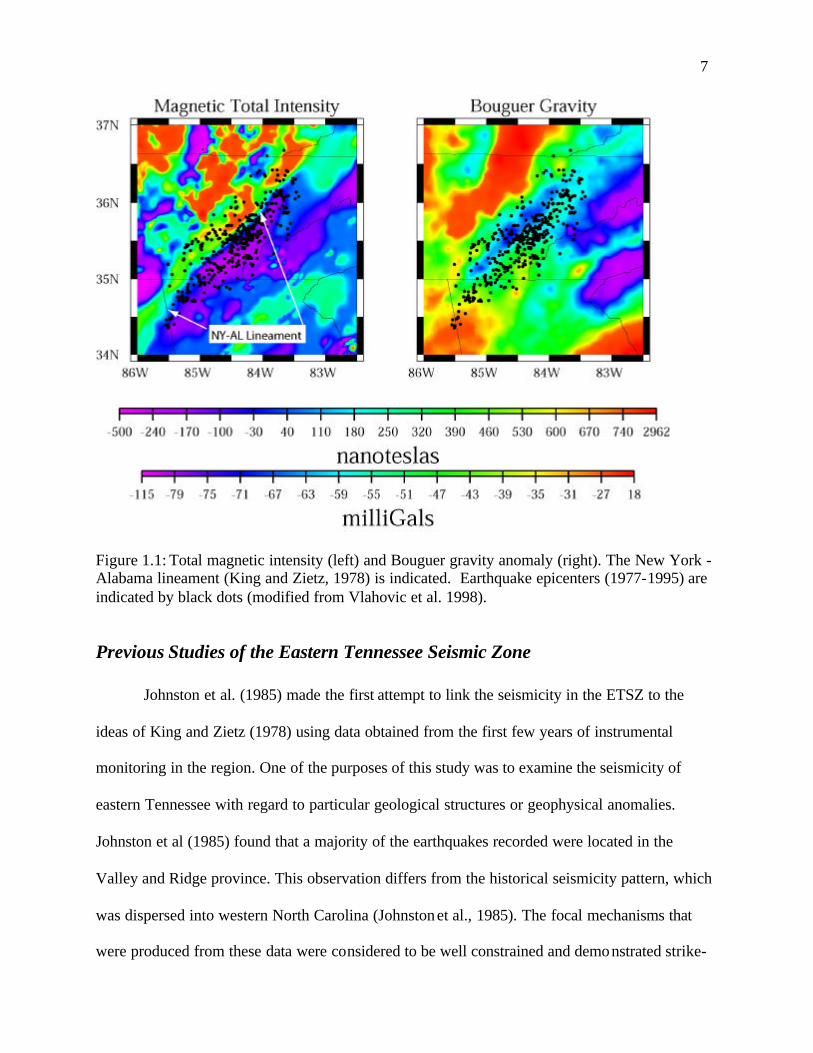
Figure 1.1: Total magnetic intensity (left) and Bouguer gravity anomaly (right). The New York - Alabama lineament (King and Zietz, 1978) is indicated. Earthquake epicenters (1977-1995) are indicated by black dots (modified from Vlahovic et al. 1998).

Previous Studies of the Eastern Tennessee Seismic Zone

Johnston et al. (1985) made the first attempt to link the seismicity in the ETSZ to the

ideas of King and Zietz (1978) using data obtained from the first few years of instrumental

monitoring in the region. One of the purposes of this study was to examine the seismicity of

eastern Tennessee with regard to particular geological structures or geophysical anomalies.

Johnston et al (1985) found that a majority of the earthquakes recorded were located in the

Valley and Ridge province. This observation differs from the historical seismicity pattern, which

was dispersed into western North Carolina (Johnston et al., 1985). The focal mechanisms that

were produced from these data were considered to be well constrained and demonstrated strike-

8

slip faulting on north-south or east-west planes (Johnston et al., 1985). Johnston et al. cited four

focal mechanisms, and the following year Teague et al. (1986) added ten more focal

mechanisms. These additional focal mechanisms agreed with the earlier observations of

Johnston et al. regarding possible fault plane orientation and slip direction. The studies of

Johnston et al (1985) and Teague et al. (1986) indicated that the seismicity in eastern Tennessee

occurs primarily in the basement, and hence may be largely unrelated to surface geology.

Johnston et al. (1985) observed very few hypocenters occurring to the northwest of the

New York-Alabama lineament. Most earthquakes were located to the southeast of the lineament,

suggesting that the magnetic lineament is the western boundary of the ETSZ (Johnston et al.,

1985). Another magnetic lineament, the Clingman/Ocoee lineament, which is less obvious than

the NY-AL lineament, appeared to mark an eastern bound of the seismicity (Johnston et al.,

1985). Johnston et al. proposed that the two lineaments are not seismogenic, but are the bounds

of a crustal block, referred to by Johnston as the Ocoee Block, that is producing the earthquakes

(1985). Johnston et al. (1985) suggest that there is a vertical lithologic difference associated with

the NY-AL lineament that corresponds with the western edge of the zone of seismicity.

The earthquake focal mechanisms and stress orientations in Eastern Tennessee were

studied by Davison (1988). He inverted eleven focal mechanisms in eastern Tennessee to derive

an estimate of the stress tensor. Davison found that the P-axes for a majority of the events

trended northeast-southwest. The estimated maximum horizontal stress direction in eastern

Tennessee was N50°E, in agreement with the previous studies of Johnston et al. (1985) and

Teague et al. (1986). Davison's (1988) results are in good agreement with Zoback and Zoback

(1988, 1991) indicating pervasive northeast trending maximum horizontal compressive stress.

Powell et al. (1994) developed a seismotectonic model based on the observed trend of

seismicity in the ETSZ. The hypothesis that was ultimately proposed is that the ETSZ is

9

narrowing into a through-going strike-slip fault, trending along the western boundary of the

Ocoee block, which coincides with the NY-AL lineament (Powell et al., 1994). The observation

of an expanded pattern of seismicity in historical times versus a narrow belt of instrumentally

located shocks suggested that seismicity in the Valley and Ridge of Tennessee is condensing

(Powell et al., 1994). Powell et al. ruled out the possibility that the apparent narrowing of the

recent seismicity was due to increased detection capability due to the seismic network. This was

tested by comparing the locations of recent shocks derived from felt reports with those of pre-

instrument shocks.

Powell et al. (1994) proposed that seismicity is occurring in the Ocoee block on North

and east striking faults that are most favorably oriented in the modern stress field. Orientations of

the nodal planes within the block are different from the northeast-southwest trend of the seismic

zone because the overall trend of the seismic zone is controlled by the subsurface orientation of

the Ocoee block (Powell et al., 1994). However, Powell et al. propose that the modern northerly

and easterly trending slip is coalescing into a northeast trending, major strike-slip zone. Powell

et al. proposed that faults within the Ocoee block may date from rifting associated with the

formation of the Iapetus Ocean and may have been modified by Paleozoic compression and

Mesozoic extension.

Kaufmann and Long (1996) looked further into the probable causes of Eastern Tennessee

seismicity. They preformed an inversion of earthquake travel time residuals to better understand

the velocity structure of the area. Two solutions were obtained. In one case, the velocity

anomalies were constrained by Bouguer gravity anomalies. In the other case, the velocity

anomalies were unconstrained. The results of the inversion led Kaufmann and Long to conclude

that earthquake hypocenters in the ETSZ were associated with low velocity zones at mid-crustal

depths. The area of the densest seismic activity, the central ETSZ, exhibited average to low

10

velocities (Kaufmann and Long 1996). Previous studies (Long and Zelt, 1991) proposed that this

central area of seismicity in the eastern Tennessee seismic zone corresponds to a zone of

weakness. Kaufmann and Long (1996) propose that this zone of weakness is due to increased

fluid content in the crust, caused by increases in porosity and fracture density. In contrast to

Johnston et al (1985), Kaufmann and Long (1996) view the New York Alabama lineament as

unrelated to the seismicity in eastern Tennessee.

Hopkins (1995) reprocessed several petroleum industry reflection profiles in eastern

Tennessee in a study that examined the New York - Alabama lineament and its possible

relationship to the Grenville Front. Hopkins interpreted the source of the magnetic anomaly as a

wedge-shaped block beneath Paleozoic sedimentary rocks in the Cumberland Plateau, which lies

to the west of the ETSZ. The base of the wedge-shaped body imaged on the reflection profiles

dips at 30 degrees to the northwest. The wedge pinches out to zero thickness beneath the location

of the steep gradient in the magnetic field. The interpretation of Hopkins, if valid, challenges

earlier conjecture by King and Zietz (1978), Johnston et al. (1985) and Powell et al (1994)

concerning the nature of the anomaly and its relationship to seismicity. Those authors assumed

that the source of the lineament is some sort of vertical lithologic contrast. Regardless of

interpretation, the data set assembled by Hopkins (1995) shows that seismicity at latitude 35.5

degrees north in the most active part of the seismic zone is occurring in rocks that are strongly

reflective. Average apparent dip on the reflection profile in this area is 35 degrees to the north.

Recently, Vlahovic et al. (1998) performed a joint hypocenter-velocity inversion for the

eastern Tennessee seismic zone in an effort to resolve features in the basement below the

Appalachian thrust sheets. This is the most recent ly developed velocity model for the region,

and is based on a data set of 492 earthquakes occurring prior to 1995. The study resolved a

strong low-velocity zone trending northeast, parallel to the seismicity. The southeastern margin

11

of the low velocity zone coincides with the NY-AL lineament. Areas of high velocity were

resolved to the southeast and northwest (Vlahovic et al., 1998). The hypocenter locations occur

mostly in a vertically bounded region approximately 30 km wide with depths of 4 to 22 km. The

northwestern vertical boundary coincides with the NY-AL lineament. The earthquakes tend to

occur in regions of average velocity or small velocity anomalies (Vlahovic et al., 1998).

In marked contrast to the interpretation of Kaufmann and Long (1996), Vlahovic et al.

(1998) proposed that earthquakes concentrate along the steepest velocity gradients. The lack of

correlation between seismicity and the regions of lowest velocity suggest that elevated pore

pressure in fluid saturated rocks is not the dominant controlling mechanism for earthquake

generation. Vlahovic et al. (1998) conclude that the earthquakes may occur on ancient faults

separating rocks of different compositions.

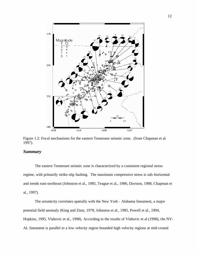
Chapman et al. (1997) examined the spatial distribution of epicenters and focal

mechanisms of earthquake in the data set used by Vlahovic et al (1998). A majority of the

earthquakes exhibited strike-slip faulting (figure 1.2). The focal mechanism nodal planes trend

predominately either north-south or east west: however, several mechanisms exhibit nodal planes

oriented northeast and northwest. The study showed statistically significant epicenter alignments

in the north-south, east-west and northeast-southwest directions, generally consistent with the

focal mechanism solutions. Chapman et al., (1997) speculate that the seismic zone is comprised

of reactivated left-stepping, en echelon, northeast striking basement faults, with intervening east-

west trending faults.

12

Figure 1.2: Focal mechanisms for the eastern Tennessee seismic zone. (from Chapman et al. 1997). Summary

The eastern Tennessee seismic zone is characterized by a consistent regional stress

regime, with primarily strike-slip faulting. The maximum compressive stress is sub-horizontal

and trends east-northeast (Johnston et al., 1985, Teague et al., 1986, Davison, 1988, Chapman et

al., 1997).

The seismicity correlates spatially with the New York - Alabama lineament, a major

potential field anomaly (King and Zietz, 1978, Johnston et al., 1985, Powell et al., 1994,

Hopkins, 1995, Vlahovic et al., 1998). According to the results of Vlahovic et al (1998), the NY-

AL lineament is parallel to a low velocity region bounded high velocity regions at mid-crustal

13

depths. They find that earthquakes tend to occur not in regions of extremely high or low

velocities, but in transitional zones between the two. Kaufmann and Long (1996) propose a

different explanation, where the seismicity is associated with a low velocity zone. The results of

Chapman et al. (1997) support the explanation of Vlahovic et al. (1998) and propose that the

velocity transitions, discussed in represent a system of northeast trending en echelon basement

faults.

Work discussed in the following chapters will attempt to test these hypotheses.

14

Chapter 2: Description of Data and Analysis Approach The data set for this study is a compilation of 993 earthquakes recorded in east

Tennessee, Alabama, Georgia, and North Carolina. The arrival time data were taken from the

Southeastern United States Seismic Network Bulletins, from 1984 through 2002. This is the

most comprehensive list of instrumentally recorded earthquakes to be considered to date for the

Eastern Tennessee Seismic Zone. The ETSZ has been monitored by the Tennessee Valley

Authority, the University of Memphis, the Georgia Institute of Technology, and the University of

Tennessee at Knoxville since the early 1980's.

The earthquakes were recorded using a network of approximately 120 vertical

component, 1Hz seismographs. It is important to note that not all of these stations were

continuously operational from 1984 through 2002. Some stations have been de-activated and

others have become operational during this period. The magnitudes of the earthquakes range

from 0.0 to 4.6. The magnitude scale used is mb(Lg), which is equivalent to the short period

teleseismic mb scale (Nuttli, 1973). Earthquakes were initially located individually using the

program Hypoellipse (Lahr, 1980). In the interest of consistency, each earthquake was located

again with hypoellipse, using only the Vlahovic et al. (1998) velocity model, unless otherwise

specifically stated.

Although the eastern Tennessee seismic zone is the most seismically active area in the

southeast, the data set for this study is small in comparison to that available for areas such as

California. In active regions, such as the San Francisco Bay region, major faults are illuminated

by recent seismicity. In comparison, far fewer earthquakes have been recorded in eastern

Tennessee, and the seismic station density is much less. Thus, relating the observed seismicity to

tectonic structures is more difficult in the ETSZ than in the San Francisco Bay area. To make

15

progress in the ETSZ, one must identify and examine small areas with the most frequent

earthquake activity. Within such areas it may be possible to derive accurate locations of one

earthquake relative to another. The basis of this study is the possibility that sufficiently accurate

relative event locations in a few small clusters will illuminate seismogenic faults. The accuracy

of individually located hypocenters is not sufficient for these purposes.

The program HYPODD (Waldhauser, 2001) will be used to identify and group clusters of

earthquakes. The program then derives relative relocations within these clusters. It has been

shown that these relative locations can greatly improve the image of seismogenic features in

situations where adequate data are available (Waldhauser and Ellsworth, 2000).

Double-Difference Algorithm

HYPODD determines relative locations within clusters using the double-difference

algorithm, developed by Waldhauser and Ellsworth (2000). Earthquakes are initially located

individually with single event programs such as Hypoellipse. These programs require an a-priori

velocity model of the crustal volume containing the hypocenters. The resulting event locations

contain errors due to un-modeled velocity structure. The double-difference algorithm can

improve relative location accuracy by removing effects due to un-modeled velocity structure.

For success, the algorithm requires that the difference between two events be small

compared to the distance between the hypocenters of the earthquakes and a station. In that case,

the travel time difference between the two events at a single station is approximately independent

of un-modeled velocity heterogeneity along the ray paths between paired events at each station.

The double difference algorithm attempts to minimize residual travel time differences, double

differences, for a pair of earthquakes at a single station. The resulting solution will be largely

free of systematic travel time errors due to velocity heterogeneity, but will retain any random

errors that were present in the original locations. For example, error due to arrival time reading

16

inaccuracies will remain in the HYPODD solutions. For that reason all attempts must be made

to reduce arrival time reading errors between event pairs.

Following Waldhauser and Ellsworth (2000), the first step in double-difference relocation

is to determine the arrival time from a point (the hypocenter) to a seismic station.

∫+=k

i

iik udsT τ (1)

The arrival time is represented by T, and is determined for one earthquake, i, to a seismic station,

k, expressed as a path integral along the ray. The origin time of event i is expressed by ti, u is

the slowness field, and ds is the element of path length.

The relationship between the travel time and the location of the event is nonlinear; it is

linearized through a Taylor expansion.

ik

iik r

t=∆

∂∂

mm

(2)

where,

( )ikcalobsik ttr −= (3)

Equation (2) relates the travel time residuals, r, for one event, i, linearly to the perturbation

vector ∆mi; which is the change in the hypocentral parameters: x,y,z, and the travel time, t. The

travel time residuals are defined as the difference between the calculated travel time (tcal) and the

observed travel time (tobs ).

These equations are relevant for only one earthquake. For the double difference

relocation to be successful there must be a relationship between two events.

ijk

ijijk dr

t=∆

∂

∂m

m (4)

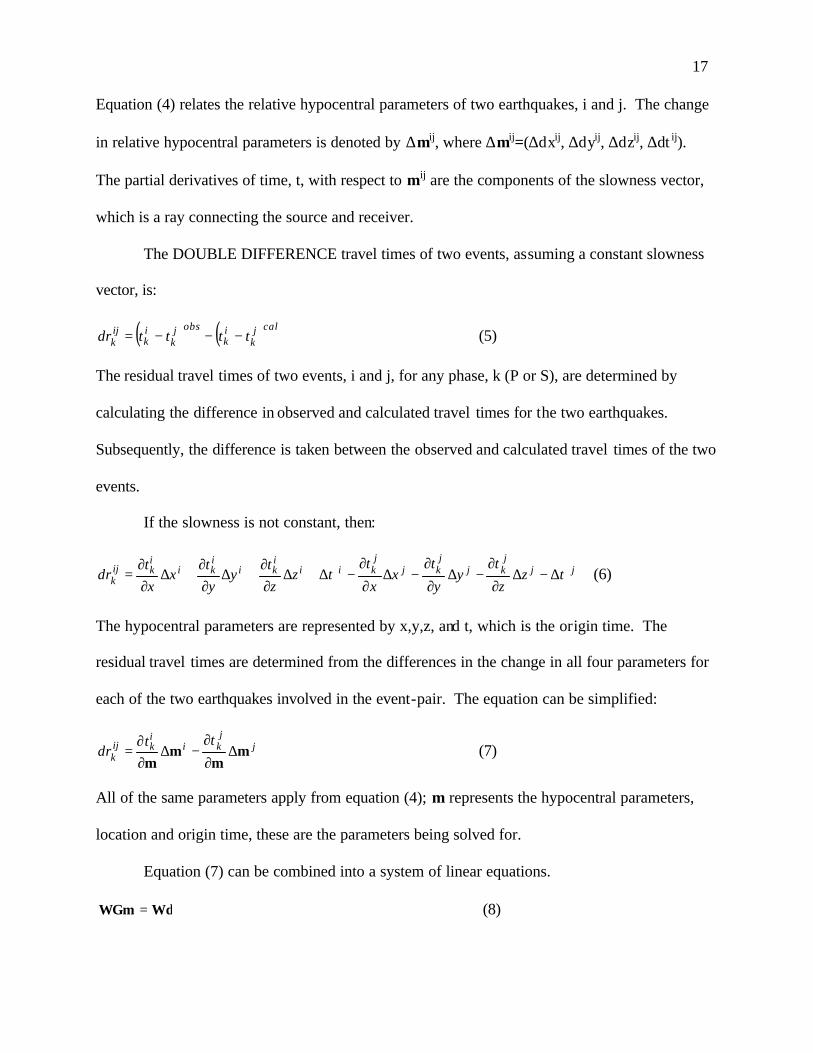
17

Equation (4) relates the relative hypocentral parameters of two earthquakes, i and j. The change

in relative hypocentral parameters is denoted by ∆mij, where ∆mij=(∆dxij, ∆dyij, ∆dzij, ∆dt ij).

The partial derivatives of time, t, with respect to mij are the components of the slowness vector,

which is a ray connecting the source and receiver.

The DOUBLE DIFFERENCE travel times of two events, assuming a constant slowness

vector, is:

( ) ( )caljk

ik

obsjk

ik

ijk ttttdr −−−= (5)

The residual travel times of two events, i and j, for any phase, k (P or S), are determined by

calculating the difference in observed and calculated travel times for the two earthquakes.

Subsequently, the difference is taken between the observed and calculated travel times of the two

events.

If the slowness is not constant, then:

jjj

kjj

kjj

kiiiki

iki

ikij

k zz

ty

y

tx

x

tz

zt

yyt

xxt

dr ττ ∆−∆∂

∂−∆

∂

∂−∆

∂

∂−∆+∆

∂∂

+∆∂∂

+∆∂∂

= (6)

The hypocentral parameters are represented by x,y,z, and t, which is the origin time. The

residual travel times are determined from the differences in the change in all four parameters for

each of the two earthquakes involved in the event-pair. The equation can be simplified:

jj

kiikij

ktt

dr mm

mm

∆∂

∂−∆

∂∂

= (7)

All of the same parameters apply from equation (4); m represents the hypocentral parameters,

location and origin time, these are the parameters being solved for.

Equation (7) can be combined into a system of linear equations.

WdWGm = (8)

18

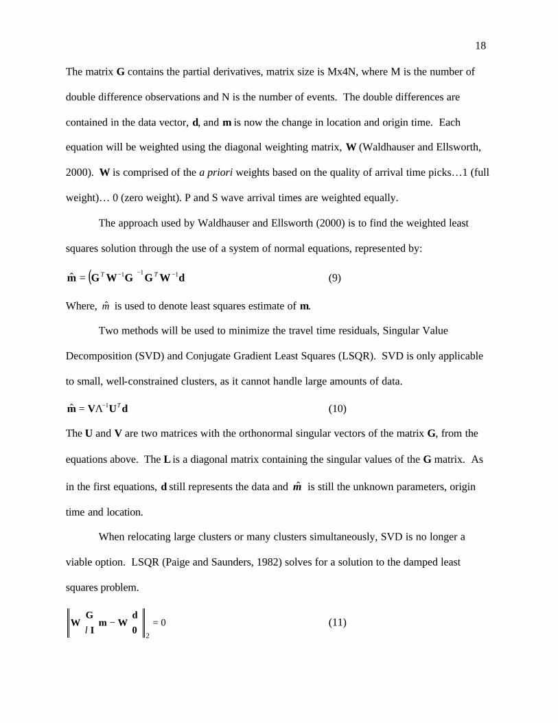
The matrix G contains the partial derivatives, matrix size is Mx4N, where M is the number of

double difference observations and N is the number of events. The double differences are

contained in the data vector, d, and m is now the change in location and origin time. Each

equation will be weighted using the diagonal weighting matrix, W (Waldhauser and Ellsworth,

2000). W is comprised of the a priori weights based on the quality of arrival time picks…1 (full

weight)… 0 (zero weight). P and S wave arrival times are weighted equally.

The approach used by Waldhauser and Ellsworth (2000) is to find the weighted least

squares solution through the use of a system of normal equations, represented by:

( ) dWGGWGm 111ˆ −−−= TT (9)

Where, m̂ is used to denote least squares estimate of m.

Two methods will be used to minimize the travel time residuals, Singular Value

Decomposition (SVD) and Conjugate Gradient Least Squares (LSQR). SVD is only applicable

to small, well-constrained clusters, as it cannot handle large amounts of data.

dUVm T1ˆ −Λ= (10)

The U and V are two matrices with the orthonormal singular vectors of the matrix G, from the

equations above. The Λ is a diagonal matrix containing the singular values of the G matrix. As

in the first equations, d still represents the data and m̂ is still the unknown parameters, origin

time and location.

When relocating large clusters or many clusters simultaneously, SVD is no longer a

viable option. LSQR (Paige and Saunders, 1982) solves for a solution to the damped least

squares problem.

02

=

−

0d

WmI

GW

λ (11)

19

When using LSQR, m still represents the location and origin time to be estimated and, I is the

identity matrix.

One of the problems faced in minimizing the travel time residuals is the sparseness of the

G matrix, since only two events are being linked together. If one event is poorly linked to

another, the G matrix can become ill conditioned, leaving the solution un-stable when using

LSQR. This problem can be dealt with by only allowing well- linked events into the solution

process; however, this becomes a problem when moderately sized clusters or data sets are being

used. LSQR deals with ill-conditioned systems by allowing damping of the solution; ? is the

damping factor in equation (11).

A well-constrained solution to the least squares problem is essential for reliable

earthquake relocations. An assessment of constraints and reliability involves sensitivity testing

of the parameters that control HYPODD, such as MAXSEP, WDCT, and DIST. This is

especially true when using a data of less than 1000 earthquakes, as well- linked events are

difficult to establish and poorly linked events must be taken into account in order to reach any

solution. This is the situation with the data set for this study.

HypoDD

In order for HYPODD to be effective, random errors must be minimized as much as

possible. In principle, cross correlations of digital waveforms can be used to reduce uncertainty

of travel time differences between earthquake pairs. Unfortunately, this is possible only for a

very few events in the eastern Tennessee seismic zone. The bulk of the travel time data are

determined from analog recordings. A major concern with analog data are reading errors in the

determination of arrival times; HYPODD cannot reduce these types of errors.

P and S wave arrivals can be used by HYPODD, either jointly or independently. In the

instance of a large data set it may be more computationally viable to perform separate relocations

20

using the P or S phases; however for this study, both phases are used jointly during each

relocation. The basic procedure behind the HYPODD relocation is to identify events that can

make an event pair, and identify the station or stations that each pair can be linked to in order to

make travel time corrections to that station; ultimately a group of event pairs are linked together

in clusters and the least squares solution for each cluster is found to achieve relative locations.

HYPODD is useful for relocation of small magnitude earthquakes; it is often used in areas with

very few large recorded earthquakes or with aftershocks of major earthquakes.

There are essentially three steps involved when relocating earthquakes with HYPODD:

1.) the forming of event pairs and links to neighbors, 2.) the formation of clusters, and 3.)

double-difference relocation. The initial step is done using the program ph2dt. Ph2dt establishes

links for each event-pair to neighboring event pairs that will ultimately determine clustering

during the next step of relocation. An event-pair are two hypocenters that fall within a pre-

defined distance of one another, and recorded at common stations. When ph2dt is run an event-

pair is linked to a certain number of neighbors to form a continuous chain of event-pairs that will

define a cluster. A neighbor is an event-pair that falls within a certain radius of another event-

pair, the MAXSEP, and meets the minimum number of phase pair links, MINLNK, established

by the program input. The MINLNK is the minimum number of phases that two pairs must

record at a single station in order to be considered neighbors. The minimum number of phase

links is typically at least eight, to allow at least one observation for the eight degrees of freedom.

In the instance that the minimum number of links is not present, a weakly linked neighbor will be

identified and may be used in relocation. These are considered the two most important criteria in

establishing a neighbor.

There are several other parameters that are used to further screen event-pairs for possible

neighbors. The MAXDIST is the maximum distance that can exist between an event pair and a

21

station; however, this parameter is typically used very liberally as there is a similar input for

HYPODD which can be used to better constrain a cluster. For very large data sets it is possible

for the large number of event pairs to exceed the limits of the computer storage and practical

limits of execution time. Ph2dt gives several options to limit the possible neighbors and phases

that will be used when running HYPODD. The most significant of these is the MAXNGH, the

maximum number of neighbors that each pair is allowed to have. An event-pair's neighbors are

listed from closest to farthest unt il the MAXNGH is reached. Also, the maximum number of

links per pair can be specified under MAXOBS. Limits imposed by small values of these last

two parameters are rarely utilized on data sets of a few thousand or less, such as in this study;

they are only necessary for data sets consisting of several thousand or more events.

Five files are created in a ph2dt run: dt.ct, dt.cc, event.sel, event.dat, and ph2dt.log. The

ph2dt.log file keeps a record of the most recent ph2dt run and pertinent information such as

weakly linked and strongly linked events; also, it records any stations not present in the station

list. The dt.ct file stores catalog data, and absolute travel time for pairs of selected earthquakes.

The dt.cc file collects differential travel times for waveform cross-correlated earthquakes, if

used. All of the events that were made available for the ph2dt program are recorded in event.dat

and the selected events are recorded in event.sel. The files that HYPODD will use are the dt.ct,

dt.cc, and event.sel; again since no cross-correlation data were used in this study, the file dt.cc

was not created or used.

After analysis using ph2dt, strongly linked event-pairs have been identified and recorded,

and can serve as input to HYPODD for the double-difference relocations. HYPODD first groups

the event-pairs into clusters. A cluster can be as small as two earthquakes (one event-pair) or as

large as the computer can computationally handle. A cluster is a continuous chain of event-pairs

that are strongly linked and meet user defined criteria set forth in the HYPODD input, by the

22

values of WDCT or DIST. It is possible and likely that two clusters may be extremely close to

each other and still be two separate clusters rather than one larger cluster. Depending on the

input parameters, HYPODD may form a few large clusters with many events in them or several

small clusters with a smaller number in each one; this is determined by the pre-specified values,

such as MAXSEP or WDCT. HYPODD can relocate all of the clusters or a selected sub-set of

clusters.

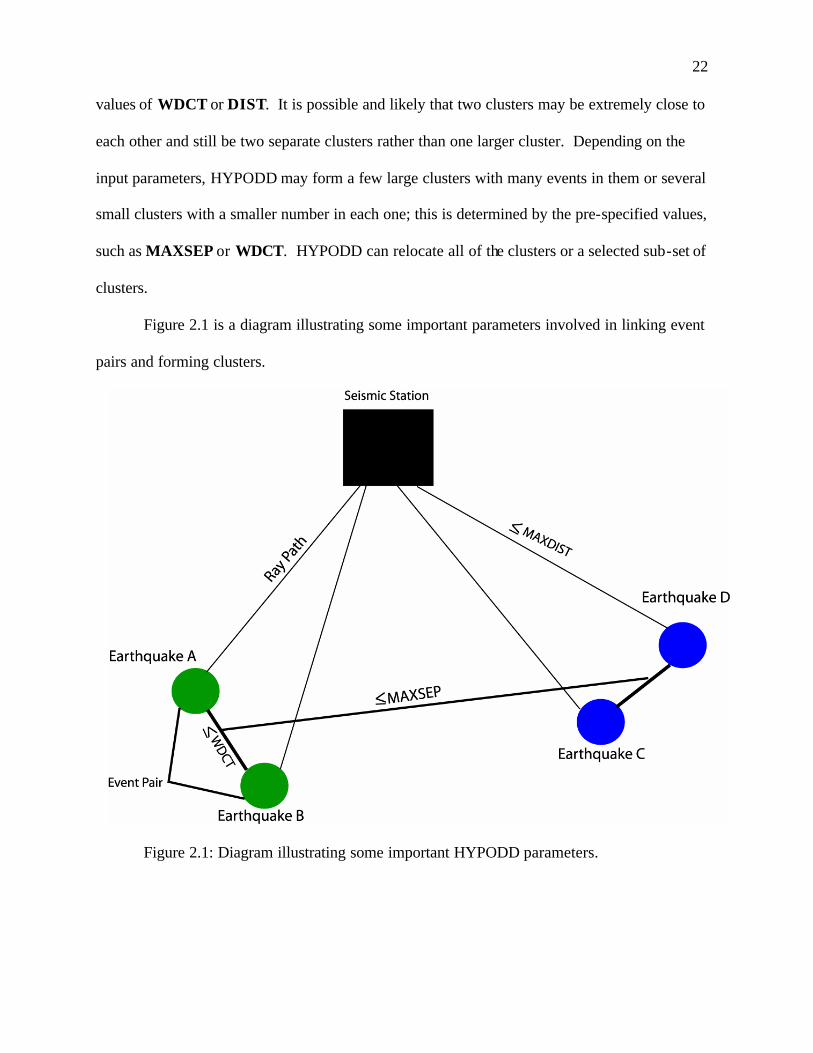
Figure 2.1 is a diagram illustrating some important parameters involved in linking event

pairs and forming clusters.

Figure 2.1: Diagram illustrating some important HYPODD parameters.

23

There are several input parameters that may be used to filter and strengthen the relocation

solution. The type of data, whether catalog or waveforms of cross-correlation data as well as

which phases (P or S, or both) are specified. One of the parameters used to define how large a

cluster will be and how many events will be included is the maximum distance between the

cluster centroid and possible stations, DIST. The larger the DIST, the more station pair-wise

corrections can be made. The clustering is actually defined by the values of OBSCC and

OBSCT, which define the minimum number of cross-correlation or catalog links, respectively,

that must be present to form a continuous chain needed to identify a cluster. Typically this

number is at least eight to account for the degrees of freedom, however, in the instance of

smaller clusters this number may be increased to sixteen or more. HYPODD gives two options

for the type of inversion to be used, singular value decomposition (SVD) or conjugate gradient

least squares (LSQR); the inversion must be identified each time HYPODD is run.

The relocation process proceeds by iterative reduction of double difference residuals.

The number of iterations is specified, considering the size of the data set and the size of the

clusters. Weights are determined for P and S waves and assigned to a certain number of

iterations. There can be any combination of the number of user specified iterations and

weighting. Also included in the iteration process are the parameters WDCT and WDCC, which

are the maximum event separation, in kilometers, for the catalog and cross-correlated data,

respectively. These parameters are similar to MAXSEP in the ph2dt program, however,

MAXSEP is the maximum distance between neighboring event-pairs and WDCT is the

maximum distance between two hypocenters to form event-pairs. Considering the similarities

between these two parameters in conjunction with the station and hypocenter spacing in eastern

Tennessee, in order to maintain consistency, MAXSEP and WDCT were always set equal to

each other in this study. Damping is used only when LSQR is the option chosen for inversion.

24

Damping is chosen for the different sets of iterations specified, between one and 100. The screen

output from HYPODD gives a condition number for each iteration and the damping should be

adapted based on this number. Waldhauser (2001) suggests that a condition number of 40-50 is

desirable when using LSQR.

The damping chosen for each HYPODD run depends on the number of clusters being

relocated and the ir size. For large clusters, or several clusters, the damping must be assigned

liberally. A major problem in relocating a large number of clusters simultaneously is that the

damping will usually be high; if the damping is too high, the relocated earthquake hypocenters

may not move. The best approach is to relocate each major cluster individually, varying the

damping for each, according to the condition number. For example, a cluster with 40

hypocenters might need a damping of 15 or 20, while, a cluster of 20 hypocenters may only need

a damping of 10 or less. Wolfe (2002) examined the trade-off involved in relocations and

damping. Wolfe found that the double-difference algorithm could successfully handle effects of

un-modeled velocity structure in earthquakes spaced close together. However, at greater

distances the need for a greater dmping value causes the relocations to be less well resolved.

The final input into HYPODD is a one-dimensional velocity model. This velocity model

can have a maximum of twelve layers. The Vp/Vs ratio is input and fixed throughout the model.

(The use of a fixed Vp/Vs ratio is a limitation of HYPODD). The P wave velocity and layer

thickness are assigned for each layer. In this study the Vp/Vs ratio is held fixed at 1.73, the P

wave travel times are held constant and the S wave travel times are varied by this ratio. The P

and S wave arrival times are weighted the same in the HYPODD input. However, the original

weights used in HYPOELLIPSE are preserved, therefore, the weighting of both P and S waves

varies. It is also important to note that the HYPOELLIPSE single-event locations calculated for

the data set did not use a constant Vp/Vs ratio, this value was varied in each layer.

25

The output from the HYPODD program is six files: hypoDD.loc, hypoDD.reloc,

hypoDD.sta, hypoDD.res, hypoDD.src, and hypoDD.log. The hypoDD.loc file contains the

individual locations before the relocations are preformed. The hypoDD.reloc file reports the

relocations in the same format as the initial locations for comparison in matlab or other visual

software. The hypoDD.sta file outputs station travel time residuals, and the hypoDD.res file

outputs double difference residuals. The hypocenter-station take-off angles are contained in

hypoDD.src, and hypoDD.log contains a summary of input and control parameters.

Another program that is included in the package with HYPODD and ph2dt is a plotting

tool for matlab, eqplot.m that is a two- dimensional program to look at epicenter location and

relocations and two possible cross-sections at specified points. This study utilizes this program

for initial inspection of relocations before inputting the locations and relocations into a 3-D

visualization package, Origin. Several tests to examine the sensitivity of the relocations to the

choices of parameter values are necessary to assess solution stability.

Example of hypoDD from Hayward Fault, California

Waldhauser and Ellsworth (2000) applied the double difference algorithm to the northern

Hayward Fault in California. The data set consisted of 346 earthquakes, ranging in magnitude

from 0.7 to 4.0, recorded between 1984 and 1998. A maximum event separation, WDCT, of 10

km was used, as well as a 200 km maximum distance between the cluster centroid and stations,

DIST; cross-correlation data were used. Two major clusters were formed and relocated. The

initial, single event locations exhibited a diffuse zone of seismicity trending to the northwest,

shown in figure 2.2. The HYPODD relocations, when performed on only the catalog data show

a much more linear northwest striking zone of earthquakes, aligned with the map fault trace, an

obvious improvement. When both the catalog and cross-correlation data are used in the

relocation, the linear features are improved in the area of dense seismicity. The sub-surface

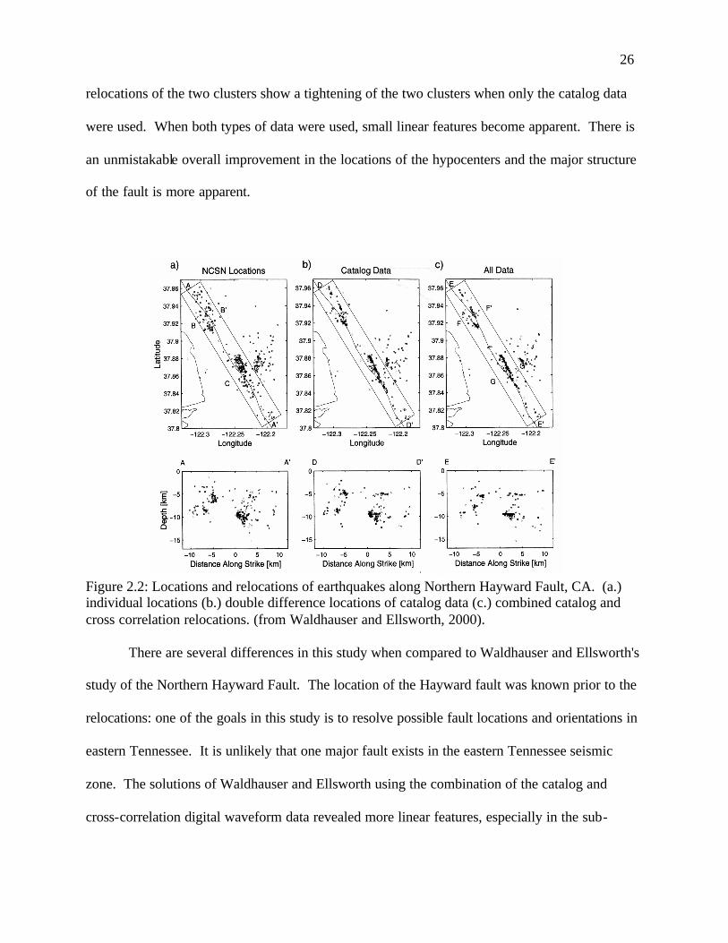
26

relocations of the two clusters show a tightening of the two clusters when only the catalog data

were used. When both types of data were used, small linear features become apparent. There is

an unmistakable overall improvement in the locations of the hypocenters and the major structure

of the fault is more apparent.

Figure 2.2: Locations and relocations of earthquakes along Northern Hayward Fault, CA. (a.) individual locations (b.) double difference locations of catalog data (c.) combined catalog and cross correlation relocations. (from Waldhauser and Ellsworth, 2000). There are several differences in this study when compared to Waldhauser and Ellsworth's

study of the Northern Hayward Fault. The location of the Hayward fault was known prior to the

relocations: one of the goals in this study is to resolve possible fault locations and orientations in

eastern Tennessee. It is unlikely that one major fault exists in the eastern Tennessee seismic

zone. The solutions of Waldhauser and Ellsworth using the combination of the catalog and

cross-correlation digital waveform data revealed more linear features, especially in the sub-

27

surface: however, this third step cannot as yet be performed in eastern Tennessee, due to the lack

of sufficient digital data.

The analysis procedure described above will be applied to the ETSZ. Hopefully the

diffuse pattern of hypocenters will condense into something that can be interpreted geologically.

28

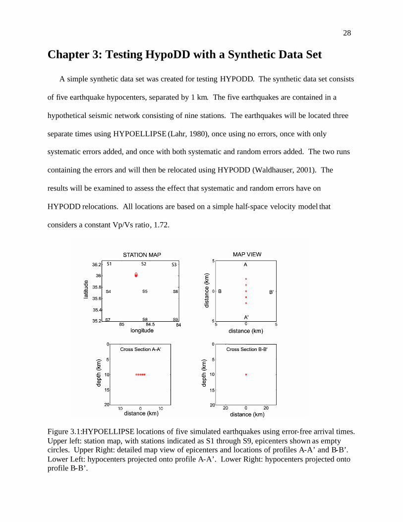
Chapter 3: Testing HypoDD with a Synthetic Data Set

A simple synthetic data set was created for testing HYPODD. The synthetic data set consists

of five earthquake hypocenters, separated by 1 km. The five earthquakes are contained in a

hypothetical seismic network consisting of nine stations. The earthquakes will be located three

separate times using HYPOELLIPSE (Lahr, 1980), once using no errors, once with only

systematic errors added, and once with both systematic and random errors added. The two runs

containing the errors and will then be relocated using HYPODD (Waldhauser, 2001). The

results will be examined to assess the effect that systematic and random errors have on

HYPODD relocations. All locations are based on a simple half-space velocity model that

considers a constant Vp/Vs ratio, 1.72.

Figure 3.1:HYPOELLIPSE locations of five simulated earthquakes using error-free arrival times. Upper left: station map, with stations indicated as S1 through S9, epicenters shown as empty circles. Upper Right: detailed map view of epicenters and locations of profiles A-A’ and B-B’. Lower Left: hypocenters projected onto profile A-A’. Lower Right: hypocenters projected onto profile B-B’.

29

Figure 3.1 shows the location of the five earthquakes with no errors. The five

earthquakes occur along a linear north-south trend, shown in map view at the top right. The top

left of figure 3.1 shows the hypothetical seismic network, the locations of the nine seismic

stations (S1 through S9), and their relation to the cluster of five earthquakes. The sub-surface

will be examined using two cross sections, A-A’ and B-B’. The hypocenters associated with

zero error are in a line at 10 kilometers depth, as shown on the north-south oriented profile A-A’.

The hypocenters appear as one point at 10 kilometers on the east-west oriented profile B-B’.

The purpose of HYPODD is to identify and correct for systematic travel time errors, thus

improving the locations of earthquake hypocenters. The ability of the program to achieve this

was tested by adding systematic error to the theoretical travel times of the error- free events,

shown in figure 3.1. The arrival times at stations S1 and S5 were made systematically early by

subtracting 0.7 seconds and the arrival times at stations S2 and S4 were made late by adding 0.7

seconds. The effects of these systematic errors on the single-event HYPOELLIPSE locations are

illustrated in figure 3.2. The epicenters were not significantly affected by the addition of the

systematic error. However, the focal depths did show significant changes; the linear trend along

cross section A-A’ (bottom left of figure 3.2) has now been distorted. The cross section B-B’

(bottom right of figure 3.2) is no longer a point, since the depths of the five earthquakes have

been affected by the errors.

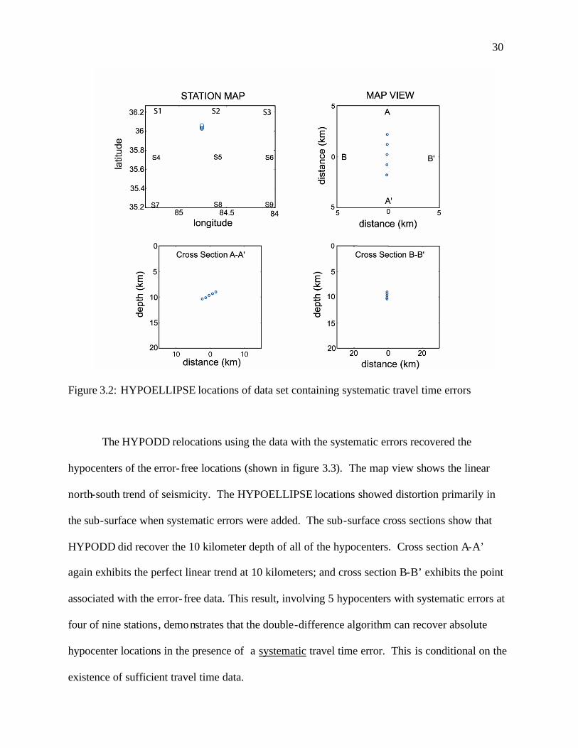
30

Figure 3.2: HYPOELLIPSE locations of data set containing systematic travel time errors

The HYPODD relocations using the data with the systematic errors recovered the

hypocenters of the error- free locations (shown in figure 3.3). The map view shows the linear

north-south trend of seismicity. The HYPOELLIPSE locations showed distortion primarily in

the sub-surface when systematic errors were added. The sub-surface cross sections show that

HYPODD did recover the 10 kilometer depth of all of the hypocenters. Cross section A-A’

again exhibits the perfect linear trend at 10 kilometers; and cross section B-B’ exhibits the point

associated with the error- free data. This result, involving 5 hypocenters with systematic errors at

four of nine stations, demonstrates that the double-difference algorithm can recover absolute

hypocenter locations in the presence of a systematic travel time error. This is conditional on the

existence of sufficient travel time data.

31

Figure 3.3: HYPODD relocations of synthetic data set with systematic errors only

In order to test HYPODD on a yet more realistic data set, random errors were added to

the same systematic errors. The random errors were drawn from a random distribution with 0

mean and a standard deviation of 0.7 seconds. The single event HYPOELLIPSE locations are

shown in figure 3.4. In map view, the north-south lineation is now more diffuse. Both cross

sections, A-A’ and B-B’, show major changes in the focal depths.

32

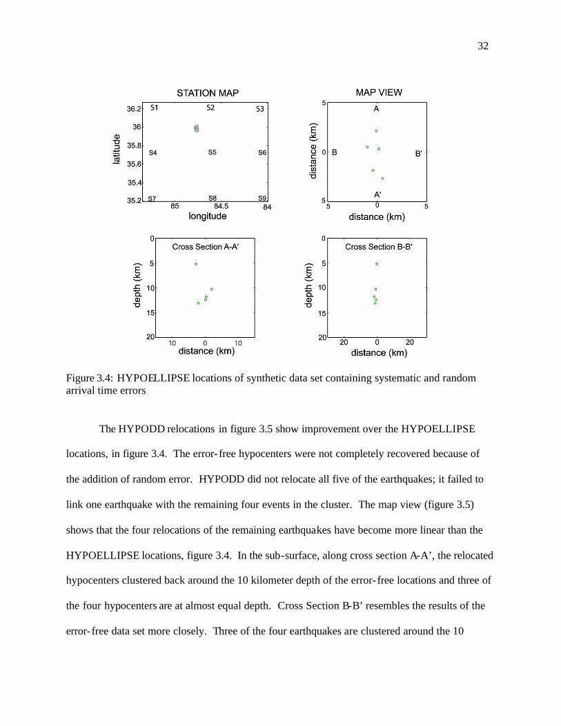
Figure 3.4: HYPOELLIPSE locations of synthetic data set containing systematic and random arrival time errors

The HYPODD relocations in figure 3.5 show improvement over the HYPOELLIPSE

locations, in figure 3.4. The error- free hypocenters were not completely recovered because of

the addition of random error. HYPODD did not relocate all five of the earthquakes; it failed to

link one earthquake with the remaining four events in the cluster. The map view (figure 3.5)

shows that the four relocations of the remaining earthquakes have become more linear than the

HYPOELLIPSE locations, figure 3.4. In the sub-surface, along cross section A-A’, the relocated

hypocenters clustered back around the 10 kilometer depth of the error- free locations and three of

the four hypocenters are at almost equal depth. Cross Section B-B’ resembles the results of the

error- free data set more closely. Three of the four earthquakes are clustered around the 10

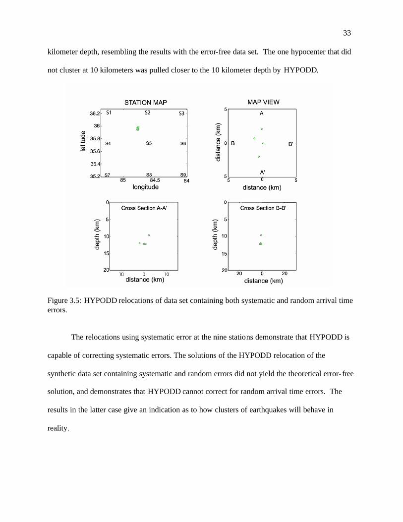
33

kilometer depth, resembling the results with the error-free data set. The one hypocenter that did

not cluster at 10 kilometers was pulled closer to the 10 kilometer depth by HYPODD.

Figure 3.5: HYPODD relocations of data set containing both systematic and random arrival time errors.

The relocations using systematic error at the nine stations demonstrate that HYPODD is

capable of correcting systematic errors. The solutions of the HYPODD relocation of the

synthetic data set containing systematic and random errors did not yield the theoretical error- free

solution, and demonstrates that HYPODD cannot correct for random arrival time errors. The

results in the latter case give an indication as to how clusters of earthquakes will behave in

reality.

34

Chapter 4: HypoDD applied to the Eastern Tennessee Seismic Zone The complete data set contains 993 earthquakes that were located using Hypoellipse

(Lahr, 1980) and the one dimensional velocity model of Vlahovic et al. (1998). A series of runs

were based on three different values of MAXSEP: 5, 10 and 20 km. The MAXSEP of five

kilometers carries the most stringent criteria to form event-pairs, neighbors, and clusters.

Larger maximum event separations (e.g., MAXSEP=20) result in the inclusion of a large

number of earthquakes in each cluster. Unfortunately, the relative locations of these events are

not substantially improved over the results obtained from HYPOELLIPSE. HYPODD is

effective when the distance between event pairs is small, compared to the earthquake-station

distance. This condition is not adequately met by the 20 km MAXSEP. Given the relatively

small number of stations and large inter-station distances, solutions using MAXSEP equal to 20

km required high damping, with the result that most relocations were not significantly changed

from original single event locations. Following the suggestion of Waldhauser and Ellsworth

(2000), a MAXSEP of 10 km was applied. Again, relatively large damping values were

required, and the largest cluster contained 280 relocated events. This suggested that optimal

results could be obtained using smaller MAXSEP. Small values of MAXSEP reduce the number

of events in the seismic zone that are relocated, but those events feature strong links. This in turn

produces improved relative event locations. The results obtained using a maximum event

separation of five kilometers will form the basis for most of the conclusions drawn in this study.

Below, I demonstrate examples of results obtained with MAXSEP values of 20 km and

10 km, and focus attention on the best event clusters resulting from relocations using a maximum

event separation of 5 km.

35

MAXSEP 20 km

The maximum event separation of twenty kilometers resulted in 628 HYPOELLIPSE

locations for input into HYPODD. HYPODD formed three clusters. The first cluster contained

most of the hypocenters, 624 events. Of those, 576 earthquakes were used in the relocation. The

remaining four earthquakes were broken into two small clusters, each containing two events,

which were not relocated successfully.

In order to achieve a marginal condition number for the solution, a high value of

damping was required. If large values of damping are required to achieve condition numbers in

the range 1 to 80, instabilility of the system of double-difference equations is indicated.

Waldhauser (2001) recommends using damping values in the range 0 to 80 in conjunction with

condition numbers in the range 40 to 80. Solution stability is usually characterized by achieving

a condition number of 40 or less with small damping values. In the case of MAXSEP 20 km, the

solution is essentially unstable, and the high damping value results in insignificant changes in the

relocations. The resulting cluster is extremely large and does not represent a useful improvement

of the original locations.

Figure 4.1 shows a plot of the epicenters from the HYPODD relocations for cluster 1,

MAXSEP 20 km. The locations are approximately the same as the original HYPOELLIPSE

locations.

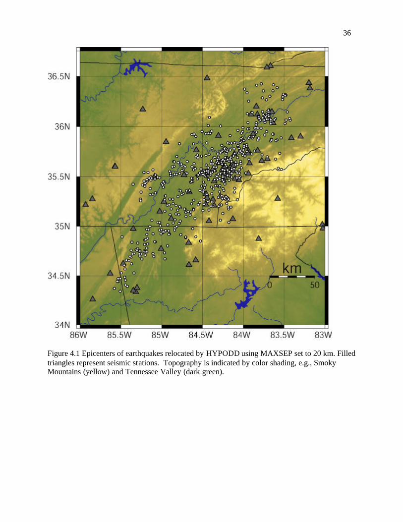
36

Figure 4.1 Epicenters of earthquakes relocated by HYPODD using MAXSEP set to 20 km. Filled triangles represent seismic stations. Topography is indicated by color shading, e.g., Smoky Mountains (yellow) and Tennessee Valley (dark green).

37

MAXSEP 10 km

The HYPODD relocations using MAXSEP 10 km formed thirty clusters, ranging in size

from almost 300 hypocenters to just two events. Most of the clusters contained very few events.

In most cases clusters containing only two events were not successfully relocated. In total, 536

HYPOELLIPSE locations formed the input data set and 507 events were relocated.

HYPODD does not relocate all events that meet the MAXSEP criteria imposed on the

data set. Events are deleted if they are not linked as a result of user-specified criteria that define

the weighting scheme used for each iteration (see Chapter 2). Also, during the interation

procedure, some events are relocated near or above the Earth's surface. The occurrence of

airquakes in small clusters can result in the entire cluster not being relocated. This problem can

be addressed by increasing damping (which prevents large fluctuation of focal depth) or by

improving spatial control (adding data from more stations near the event cluster). HYPODD

removes airquakes and then relocates the remaining events in a given cluster.

Cluster 1, MAXSEP 10:

For MAXSEP 10 km, eleven clusters formed that contained five or more events. The

largest cluster, cluster 1, contained 298 single-event locations. In cluster 1, 280 events were

relocated with a final damping value of 45 and corresponding condition number of 45. Two

other clusters have 40 or more relocated events. The remaining clusters have many fewer events

and lack earthquakes with focal mechanism solutions. Table 4.1 lists cluster number, the

geographic coordinates of the cluster-corner points, the number of HYPOELLIPSE single event

locations, and the damping and condition number of final iteration. Figure 4.2 plots the events in

the six largest clusters.

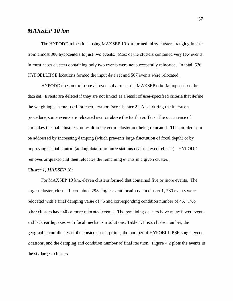
38

Figure 4.2 Locations of the six largest clusters, MAXSEP 10 km. Each epicenter cluster is indicated by numbers, 1(red), 2(yellow), 3(white), 4, 5, and 6 (black). Station locations are represented by triangles. Topography is indicated by color shading, e.g., Smoky Mountains (yellow) and Tennessee Valley (dark green).

The earthquakes comprising cluster 1 represent the most dense concentration of

seismicity in the eastern Tennessee Seismic Zone, and for that reason cluster 1 can be expected

to offer the best opportunity for the double difference algorithm to improve the locations.

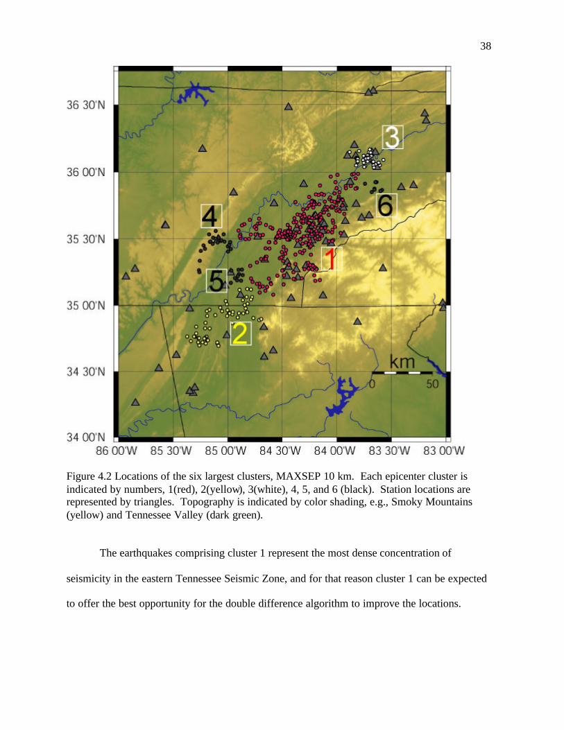
39

Figure 4.3. Comparison of HYPOELLIPSE original epicenters with those relocated in Cluster 1 using MAXSEP 10 km. The latitude and longitude of the corner points of the cluster are indicated on the top plot. Numbers correspond to focal mechanisms, listed in Table 4.2.

Figure 4.3 (above) compares the original HYPOELLIPSE epicenter locations for cluster

1 to the relocations derived using MAXSEP 10 km. Figure 4.4 (below) shows a perspective plot

of the original hypocenters in cluster 1 and those relocated with HYPODD, using MAXSEP 10.

40

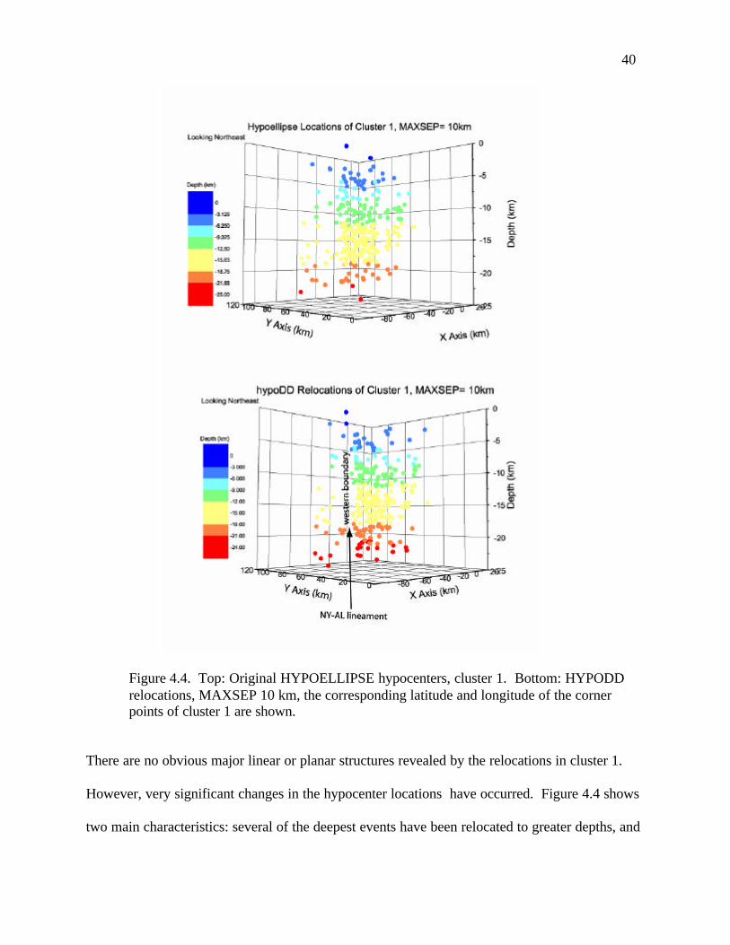
Figure 4.4. Top: Original HYPOELLIPSE hypocenters, cluster 1. Bottom: HYPODD relocations, MAXSEP 10 km, the corresponding latitude and longitude of the corner points of cluster 1 are shown.

There are no obvious major linear or planar structures revealed by the relocations in cluster 1.

However, very significant changes in the hypocenter locations have occurred. Figure 4.4 shows

two main characteristics: several of the deepest events have been relocated to greater depths, and

41

there is an obvious "tightening" of the relocated hypocenters. In figure 4.4 the northwestern

margin of cluster 1 has been sharply defined by the relocations as a vertical boundary between

seismogenic crust and relatively aseismic crust.

The mean change in the hypocenter locations for cluster 1 is 2.1 km, the mean absolute

value of the change in depth is 1.7 km, and the mean horizontal shift is 1.0 km. The mean

change in focal depth is only 0.2 km with the relocations on average being slightly deeper.

However, particular events were shifted considerably. The maximum change in depth was 11.5

km and the maximum change in a horizontal direction was 3.6 km. The ten and ninety percentile

changes in the hypocenter relocations were 0.7 km and 3.98 km respectively.

Table 4.1 Breakdown of Clusters Analyzed using MAXSEP 10 km Cluster Number

Number of Events

Damping Value

Condition Number (last iteration)

Geographic Coordinates Of Corner Points °N °W

1 298 45 45 36.08 36.10 35.00 35.00

85.10 83.67 85.10 83.67

2 63 25 30 35.35 35.35 34.64 34.64

85.47 84.60 85.47 84.60

3 27 15 36 36.40 36.40 35.99 35.99

84.00 83.50 84.00 83.50

4 11 15 15 35.63 35.63 35.22 35.22

84.94 85.21 84.94 85.21

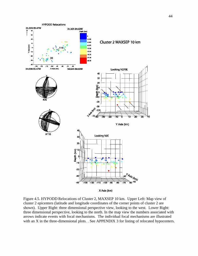
Cluster 2, MAXSEP 10:

The relocated hypocenters for cluster 2 are shown in figure 4.5, below. Cluster 2 consists

of 56 relocated earthquakes. Two focal mechanisms (Chapman et al., 1997) are available from

42

among events in this cluster and are shown in figure 4.5. My strategy is to use the focal

mechanisms as a guide for examining the three dimensional spatial characteristics of the

HYPODD relocations. Therefore, I have created a series of three dimensional plots aligned with

the strike directions of the focal mechanism nodal planes. Table 4.2 identifies and outlines the

location, strike, dip, and rake of the focal mechanisms examine with each cluster. The focal

mechanisms available for cluster 2 indicate northerly and easterly striking nodal planes. When

viewed in perspective, looking to the west, the relocated hypocenters suggest at least two

possible northerly dipping planes. This interpretation is equivocal: however, it is consistent with

focal mechanism #116. When the hypocenter view is oriented in a northerly direction, the

pattern of hypocenters does not suggest planar features. Based upon the available information, I

interpret the available information as suggesting that the seismogenic structures in cluster 2 may

strike to the west and dip to the north.

The mean change in the hypocenter locations is 2.4 km. The mean change in a horizontal

direction was 1.0 km and the mean change in the depth was 2.0 km. The range of hypocenter

depths is approximately from 1 to 24 km. A majority of the events after relocation are at depths

less than 10 km (figure 4.5).

43

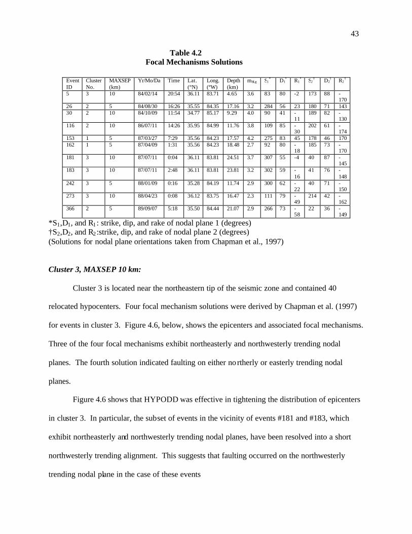
Table 4.2 Focal Mechanisms Solutions

*S1,D1, and R1 : strike, dip, and rake of nodal plane 1 (degrees) †S2,D2, and R2 :strike, dip, and rake of nodal plane 2 (degrees) (Solutions for nodal plane orientations taken from Chapman et al., 1997)

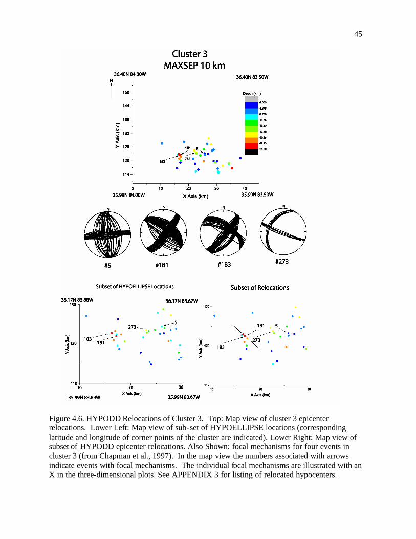
Cluster 3, MAXSEP 10 km:

Cluster 3 is located near the northeastern tip of the seismic zone and contained 40

relocated hypocenters. Four focal mechanism solutions were derived by Chapman et al. (1997)

for events in cluster 3. Figure 4.6, below, shows the epicenters and associated focal mechanisms.

Three of the four focal mechanisms exhibit northeasterly and northwesterly trending nodal

planes. The fourth solution indicated faulting on either northerly or easterly trending nodal

planes.

Figure 4.6 shows that HYPODD was effective in tightening the distribution of epicenters

in cluster 3. In particular, the subset of events in the vicinity of events #181 and #183, which

exhibit northeasterly and northwesterly trending nodal planes, have been resolved into a short

northwesterly trending alignment. This suggests that faulting occurred on the northwesterly

trending nodal plane in the case of these events

Event ID

Cluster No.

MAXSEP (km)

Yr/Mo/Da Time Lat. (°N)

Long. (°W)

Depth (km)

mbLg S1* D1

* R1* S2

† D2† R2

†

5 3 10 84/02/14 20:54 36.11 83.71 4.65 3.6 83 80 -2 173 88 -170

26 2 5 84/08/30 16:26 35.55 84.35 17.16 3.2 284 56 23 180 71 143 30 2 10 84/10/09 11:54 34.77 85.17 9.29 4.0 90 41 -

11 189 82 -

130 116 2 10 86/07/11 14:26 35.95 84.99 11.76 3.8 109 85 -

30 202 61 -

174 153 1 5 87/03/27 7:29 35.56 84.23 17.57 4.2 275 83 45 178 46 170 162 1 5 87/04/09 1:31 35.56 84.23 18.48 2.7 92 80 -

18 185 73 -

170 181 3 10 87/07/11 0:04 36.11 83.81 24.51 3.7 307 55 -4 40 87 -

145 183 3 10 87/07/11 2:48 36.11 83.81 23.81 3.2 302 59 -

16 41 76 -

148 242 3 5 88/01/09 0:16 35.28 84.19 11.74 2.9 300 62 -

22 40 71 -

150 273 3 10 88/04/23 0:08 36.12 83.75 16.47 2.3 111 79 -

49 214 42 -

162 366 2 5 89/09/07 5:18 35.50 84.44 21.07 2.9 266 73 -

58 22 36 -

149

44

Figure 4.5. HYPODD Relocations of Cluster 2, MAXSEP 10 km. Upper Left: Map view of cluster 2 epicenters (latitude and longitude coordinates of the corner points of cluster 2 are shown). Upper Right: three dimensional perspective view, looking to the west. Lower Right: three dimensional perspective, looking to the north. In the map view the numbers associated with arrows indicate events with focal mechanisms. The individual focal mechanisms are illustrated with an X in the three-dimensional plots. . See APPENDIX 3 for listing of relocated hypocenters.

45

Figure 4.6. HYPODD Relocations of Cluster 3. Top: Map view of cluster 3 epicenter relocations. Lower Left: Map view of sub-set of HYPOELLIPSE locations (corresponding latitude and longitude of corner points of the cluster are indicated). Lower Right: Map view of subset of HYPODD epicenter relocations. Also Shown: focal mechanisms for four events in cluster 3 (from Chapman et al., 1997). In the map view the numbers associated with arrows indicate events with focal mechanisms. The individual focal mechanisms are illustrated with an X in the three-dimensional plots. See APPENDIX 3 for listing of relocated hypocenters.

46

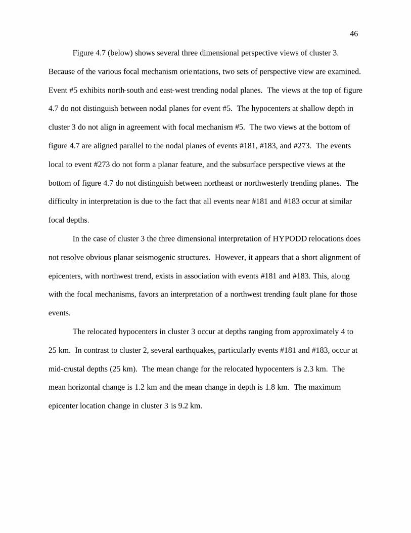
Figure 4.7 (below) shows several three dimensional perspective views of cluster 3.

Because of the various focal mechanism orientations, two sets of perspective view are examined.

Event #5 exhibits north-south and east-west trending nodal planes. The views at the top of figure

4.7 do not distinguish between nodal planes for event #5. The hypocenters at shallow depth in

cluster 3 do not align in agreement with focal mechanism #5. The two views at the bottom of

figure 4.7 are aligned parallel to the nodal planes of events #181, #183, and #273. The events

local to event #273 do not form a planar feature, and the subsurface perspective views at the

bottom of figure 4.7 do not distinguish between northeast or northwesterly trending planes. The

difficulty in interpretation is due to the fact that all events near #181 and #183 occur at similar

focal depths.

In the case of cluster 3 the three dimensional interpretation of HYPODD relocations does

not resolve obvious planar seismogenic structures. However, it appears that a short alignment of

epicenters, with northwest trend, exists in association with events #181 and #183. This, along

with the focal mechanisms, favors an interpretation of a northwest trending fault plane for those

events.

The relocated hypocenters in cluster 3 occur at depths ranging from approximately 4 to

25 km. In contrast to cluster 2, several earthquakes, particularly events #181 and #183, occur at

mid-crustal depths (25 km). The mean change for the relocated hypocenters is 2.3 km. The

mean horizontal change is 1.2 km and the mean change in depth is 1.8 km. The maximum

epicenter location change in cluster 3 is 9.2 km.

47

Figure 4.7. Hypocenter relocations of cluster 3. Top Left: three dimensional perspective oriented north. Top Right: Perspective view oriented west. Bottom Left: Perspective oriented northeast. Bottom Right: Perspective oriented northwest. Also Shown: focal mechanisms for four events in cluster 3 (from Chapman et al., 1997). In the map view the numbers associated with arrows indicate events with focal mechanisms. The individual focal mechanisms are illustrated with an X in the three-dimensional plots. See APPENDIX 3 for listing of relocated hypocenters.

48

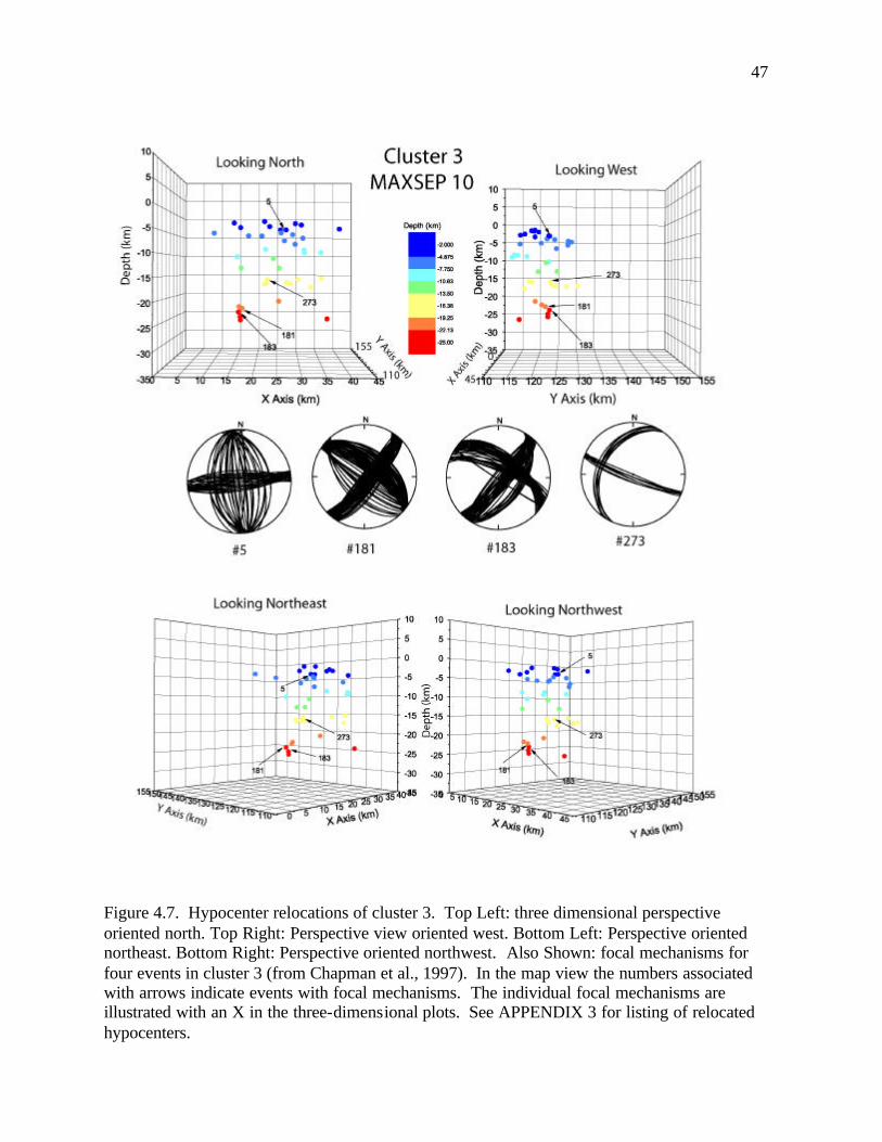
Clusters 4, 5, and 6, MAXSEP 10 km:

Clusters 5 and 6 do not contain enough events for meaningful geologic interpretation.

Cluster 4 is interesting because it lies to the west of the NY-AL lineament. Unfortunately, there

are no focal mechanism solutions for this cluster. Figure 4.8 shows the HYPOELLIPSE single

event locations and HYPODD relocations of the hypocenters. The relocations produced

somewhat greater focal depths in this cluster. It is interesting to note that most of the events,

more than 50 percent, occurred between 15 and 25 km, whereas, at least 50% of the events in

clusters 1,2, and 3 are shallow events (depths less than 15 km).

Figure 4.8. Comparison of HYPOELLIPSE single event locations and HYPODD relocations of cluster 4. Left: three dimensional plot of HYPOELLIPSE locations looking to the west. Right: HYPODD relocations.

49

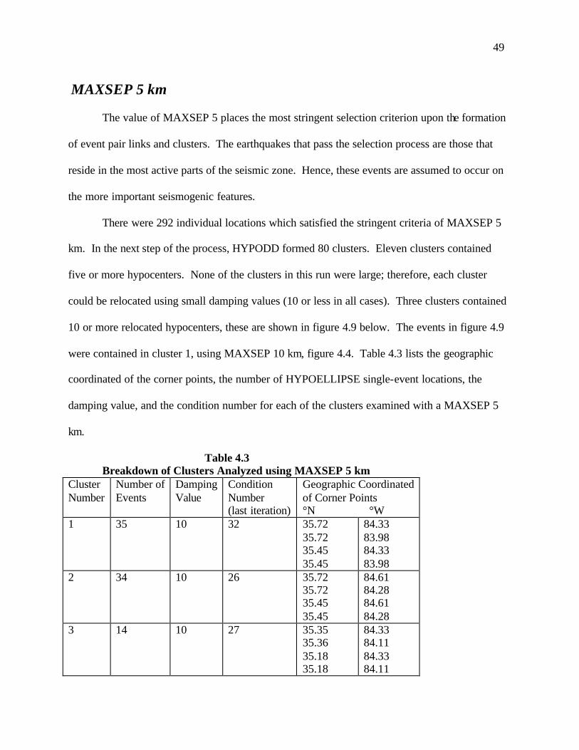
MAXSEP 5 km The value of MAXSEP 5 places the most stringent selection criterion upon the formation

of event pair links and clusters. The earthquakes that pass the selection process are those that

reside in the most active parts of the seismic zone. Hence, these events are assumed to occur on

the more important seismogenic features.

There were 292 individual locations which satisfied the stringent criteria of MAXSEP 5

km. In the next step of the process, HYPODD formed 80 clusters. Eleven clusters contained

five or more hypocenters. None of the clusters in this run were large; therefore, each cluster

could be relocated using small damping values (10 or less in all cases). Three clusters contained

10 or more relocated hypocenters, these are shown in figure 4.9 below. The events in figure 4.9

were contained in cluster 1, using MAXSEP 10 km, figure 4.4. Table 4.3 lists the geographic

coordinated of the corner points, the number of HYPOELLIPSE single-event locations, the

damping value, and the condition number for each of the clusters examined with a MAXSEP 5

km.

Table 4.3 Breakdown of Clusters Analyzed using MAXSEP 5 km Cluster Number

Number of Events

Damping Value

Condition Number (last iteration)

Geographic Coordinated of Corner Points °N °W

1 35 10 32 35.72 35.72 35.45 35.45

84.33 83.98 84.33 83.98

2 34 10 26 35.72 35.72 35.45 35.45

84.61 84.28 84.61 84.28

3 14 10 27 35.35 35.36 35.18 35.18

84.33 84.11 84.33 84.11

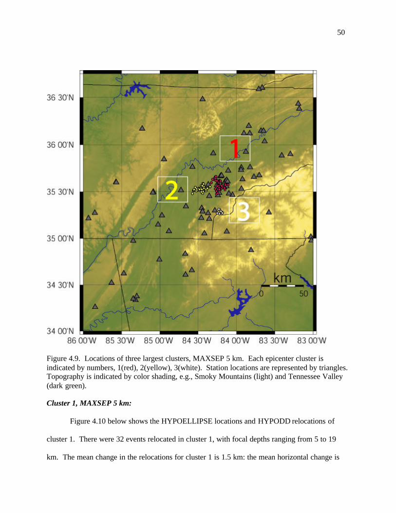
50

Figure 4.9. Locations of three largest clusters, MAXSEP 5 km. Each epicenter cluster is indicated by numbers, 1(red), 2(yellow), 3(white). Station locations are represented by triangles. Topography is indicated by color shading, e.g., Smoky Mountains (light) and Tennessee Valley (dark green). Cluster 1, MAXSEP 5 km:

Figure 4.10 below shows the HYPOELLIPSE locations and HYPODD relocations of

cluster 1. There were 32 events relocated in cluster 1, with focal depths ranging from 5 to 19

km. The mean change in the relocations for cluster 1 is 1.5 km: the mean horizontal change is

51

0.7 km, and the mean change in depth is 1.2 km. The maximum horizontal change is 5.3 km and

the maximum change in depth is 4.9 km. These changes represent approximately half of the

values encountered when relocating the events in clusters described above using MAXSEP 10

km. Note that because of the selection criteria (MAXSEP 5 km), these events sample the most

active parts of the ETSZ.

Two focal mechanisms were calculated for cluster 1 by Chapman et al. (1997). These

mechanisms exhibit strike-slip faulting, with north-south and east-west trending nodal planes.

Event #153 was the magnitude 4.2, Vonore, TN earthquake; which is the third largest earthquake

to have been instrumentally recorded in the seismic zone and the largest earthquake included in

this data set. The Vonore earthquake produced an aftershock sequence that was monitored by a

temporary local network (Nava et al., 1989). Nava et al. inferred unilateral rupture on a north-

south nodal plane, based on location of the main shock and a sub-set of nearby aftershocks

recorded using the temporary network. Nine aftershock epicenters were located within 3.5 km of

the main shock and 6 of those aftershocks formed a north-south trending alignment with the

main shock. However, as noted by Chapman et al. (1997), 12 additional "aftershocks" occurred

at distances up to 50 km from the main shock and lie generally on an east-west alignment with

the epicenter of the main shock. Event #162 was the largest of the local aftershocks and the only

one recorded well by the permanent network, therefore, it is the only aftershock considered in

this data set.

The three dimensional plots of cluster 1, figure 4.10, are oriented along the two nodal

plane strike directions for events #153 and #162. Both the map view for the epicenters and the

perspective view looking to the north support the conclusion of Nava et al. (1989), that faulting

occurred on the north trending nodal plane. In Figure 4.10 there is an east-west trend of

epicenters at Y coordinate value 63, extending from X coordinates -23 km to -12 km. In

52

perspective view to the west, the hypocenters local to events #153 and #162 suggest a northerly

dipping planar feature. The dip of the westerly trending nodal plane of #153 is 83 degrees. The

dip of event #162 is steep, but not well constrained. On the basis of the data in cluster 1, the

HYPODD relocations fail to distinguish between the two possible fault orientations.

Cluster 2, MAXSEP 5 km:

Cluster 2 is located directly to the west of cluster 1 (figure 4.9). HYPODD relocated 34

events in this cluster. Figure 4.11 shows the HYPOELLIPSE locations and HYPODD

relocations of cluster 2. The relocated focal depths in this cluster range from 8 to 22 km. The

mean change in location in cluster 2 was 2.2 km. The mean horizontal change was 1.4 km and

the mean change in depth was also 1.4 km. The maximum horizontal change in this cluster was

13.8 km and the maximum change in depth was 3.9 km. The mean changes for cluster 2 are

approximately twice as large as cluster 1.

Two focal mechanisms were calculated for cluster 2 (Chapman et al., 1997). Event #366

shows a west trending, steeply dipping nodal plane; and a northerly trending, shallow dipping

nodal plane. Event #26, on the western edge of the cluster, also has north-south and east-west

trending nodal planes, with a steep dip on the northerly plane and a 56 degree dip on the east-

west nodal plane.

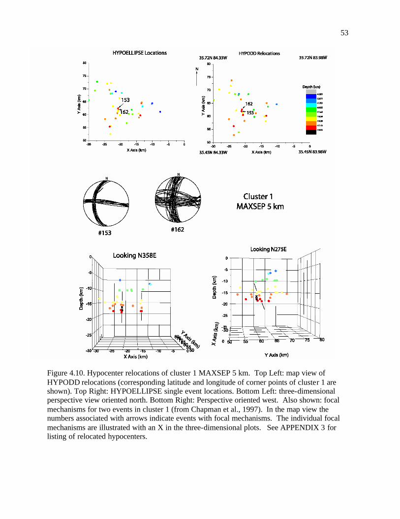
53

Figure 4.10. Hypocenter relocations of cluster 1 MAXSEP 5 km. Top Left: map view of HYPODD relocations (corresponding latitude and longitude of corner points of cluster 1 are shown). Top Right: HYPOELLIPSE single event locations. Bottom Left: three-dimensional perspective view oriented north. Bottom Right: Perspective oriented west. Also shown: focal mechanisms for two events in cluster 1 (from Chapman et al., 1997). In the map view the numbers associated with arrows indicate events with focal mechanisms. The individual focal mechanisms are illustrated with an X in the three-dimensional plots. See APPENDIX 3 for listing of relocated hypocenters.

54

Event #26 was magnitude 3.2 and event #366 was magnitude 2.9. Generally, the cluster trends

east-west, which is parallel to one nodal plane of both focal mechanisms. This is significant,

because the cluster represents, based on the selection criteria, one of the most seismically active

areas in the seismic zone. Events on the western end of the cluster tend to be more shallow than

the events occurring on the eastern edge.

The three-dimensional perspectives are oriented along the two nodal planes of the focal

mechanisms. The perspective oriented to the north suggests a diffuse planar feature with shallow

dip to the east. The perspective oriented to the west suggests a diffuse planar feature dipping

more steeply to the north. Of the two possibilities suggested by the available data, I interpret the

more likely case to be that represented by the west striking, north dipping feature. My reason for

this interpretation is that both focal mechanisms suggest a steeply dipping, west striking, nodal

plane. Whereas, focal mechanism #26 does not support a shallow dipping north striking fault

plane.

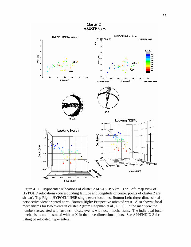
55

Figure 4.11. Hypocenter relocations of cluster 2 MAXSEP 5 km. Top Left: map view of HYPODD relocations (corresponding latitude and longitude of corner points of cluster 2 are shown). Top Right: HYPOELLIPSE single event locations. Bottom Left: three-dimensional perspective view oriented north. Bottom Right: Perspective oriented west. Also shown: focal mechanisms for two events in cluster 2 (from Chapman et al., 1997). In the map view the numbers associated with arrows indicate events with focal mechanisms. The individual focal mechanisms are illustrated with an X in the three-dimensional plots. See APPENDIX 3 for listing of relocated hypocenters.

56

Cluster 3, MAXSEP 5 km:

Cluster 3 is located on the Tennessee-North Carolina border, figure 4.9. The cluster

consists of 14 HYPOELLIPSE single event locations, all of which were relocated by HYPODD.

Figure 4.12 shows the HYPOELLIPSE locations and the HYPODD relocations of cluster

3. The hypocenters in this cluster range in depth from 7 to 17 km. The mean change in the

relocated hypocenters for cluster 3 is 2.3 km. The mean horizontal change is 0.6 km and the

mean change in depth is 1.3 km. The maximum horizontal change for cluster 3 is 1.1 km and the

maximum change is depth is 4.6 km. The HYPODD relocations of cluster 3 resolved a linear

trend of epicenters.

There was one focal mechanism calculated for cluster 3 (Chapman et al., 1997). This

event was a magnitude 2.9 earthquake. Event #242 is not a well constrained focal mechanism.

However, the northwest trending nodal plane agrees perfectly with the linear trend of epicenters

resolved by HYPODD. On the basis of this excellent correspondence, I conclude that the fault

corresponds to the steeply dipping northwest trending plane.

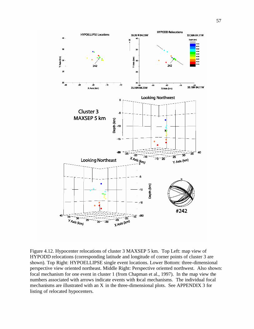
57

Figure 4.12. Hypocenter relocations of cluster 3 MAXSEP 5 km. Top Left: map view of HYPODD relocations (corresponding latitude and longitude of corner points of cluster 3 are shown). Top Right: HYPOELLIPSE single event locations. Lower Bottom: three-dimensional perspective view oriented northeast. Middle Right: Perspective oriented northwest. Also shown: focal mechanism for one event in cluster 1 (from Chapman et al., 1997). In the map view the numbers associated with arrows indicate events with focal mechanisms. The individual focal mechanisms are illustrated with an X in the three-dimensional plots. See APPENDIX 3 for listing of relocated hypocenters.

58

Combined Subset of Clusters 1 and 2, MAXSEP 5 km:

Clusters 1 and 2 represent adjacent areas of the densest seismic activity within the eastern

Tennessee seismic zone. The area of densest activity is represented by two clusters, rather than

one, because a small gap exceeding 5 km broke the chain that would have linked the two into

one cluster. Therefore, I will examine both clusters simultaneously. There were two focal

mechanisms calculated for each cluster (Chapman et al., 1997). The two focal mechanisms in

cluster 1, #153 and #162, are located in the western portion of the cluster. The two focal

mechanisms for cluster 2, #26 and #366, are located near the eastern edge of that cluster. In

order to examine the spatial distribution of hypocenters in the vicinity of the events with focal

mechanisms, I combine a subset of events from both clusters. The events included those in the

western section of cluster 1 and those in the eastern section of cluster 2. Figure 4.13 shows the

HYPODD relocations of these events in map-view and in three-dimensions.

Within the subset are the four focal mechanisms associated with the two clusters. The

four focal mechanisms discussed in each cluster contained nodal planes trending to the north and

west. The dips of the north-south trending nodal planes range from shallow dip to the east (event

#366), to steep dip to the west (event #153). The east-west trending nodal planes of the four

focal mechanisms show better agreement in terms of consistent dip to the north. Therefore, I

favor the east-west trending nodal plane as a potential fault plane for all four mechanisms. This

interpretation is strengthened by the overall east-west trend of the epicenters, as shown in map

view at the top of figure 4.13. This interpretation appears consistent with the perspective plots

shown at the bottom of figure 4.13. The view looking north shows no obvious planar features.

However, the view looking west does suggest a west striking, north dipping, planar concentration

of hypocenters. The dip, inferred from figure 4.13, is approximately 50 degrees. This

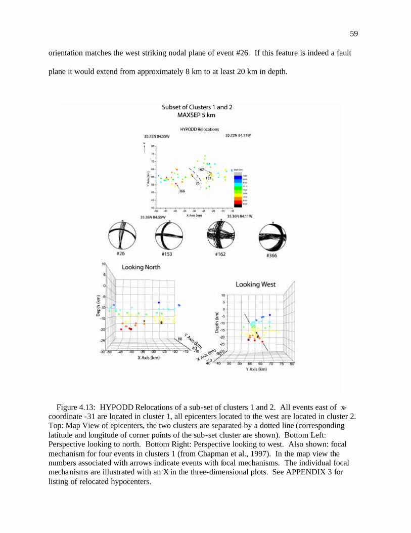
59

orientation matches the west striking nodal plane of event #26. If this feature is indeed a fault

plane it would extend from approximately 8 km to at least 20 km in depth.

Figure 4.13: HYPODD Relocations of a sub-set of clusters 1 and 2. All events east of x-coordinate -31 are located in cluster 1, all epicenters located to the west are located in cluster 2. Top: Map View of epicenters, the two clusters are separated by a dotted line (corresponding latitude and longitude of corner points of the sub-set cluster are shown). Bottom Left: Perspective looking to north. Bottom Right: Perspective looking to west. Also shown: focal mechanism for four events in clusters 1 (from Chapman et al., 1997). In the map view the numbers associated with arrows indicate events with focal mechanisms. The individual focal mechanisms are illustrated with an X in the three-dimensional plots. See APPENDIX 3 for listing of relocated hypocenters.

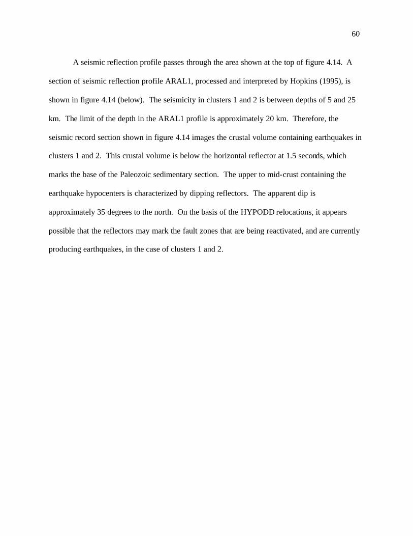
60

A seismic reflection profile passes through the area shown at the top of figure 4.14. A

section of seismic reflection profile ARAL1, processed and interpreted by Hopkins (1995), is

shown in figure 4.14 (below). The seismicity in clusters 1 and 2 is between depths of 5 and 25

km. The limit of the depth in the ARAL1 profile is approximately 20 km. Therefore, the

seismic record section shown in figure 4.14 images the crustal volume containing earthquakes in

clusters 1 and 2. This crustal volume is below the horizontal reflector at 1.5 seconds, which

marks the base of the Paleozoic sedimentary section. The upper to mid-crust containing the

earthquake hypocenters is characterized by dipping reflectors. The apparent dip is

approximately 35 degrees to the north. On the basis of the HYPODD relocations, it appears

possible that the reflectors may mark the fault zones that are being reactivated, and are currently

producing earthquakes, in the case of clusters 1 and 2.

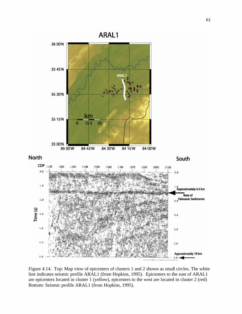
61

Figure 4.14. Top: Map view of epicenters of clusters 1 and 2 shown as small circles. The white line indicates seismic profile ARAL1 (from Hopkins, 1995). Epicenters to the east of ARAL1 are epicenters located in cluster 1 (yellow), epicenters to the west are located in cluster 2 (red) Bottom: Seismic profile ARAL1 (from Hopkins, 1995).

62

Sensitivity Testing of hypoDD:

There were two tests done on HYPODD to test for its sensitivity to different input

velocity models.

In the first test, I compared the HYPODD relocations described above, with those

developed using a different velocity model for single event location. The individual events were

located using a velocity model developed for Giles County, Virginia instead of the velocity

model developed by Vlahovic et al, (1998). The Giles County velocity model contains four

layers, as opposed to the six layers used by Vlahovic et al. (1998). These single-event locations

were then relocated with HYPODD, using MAXSEP 5 km. The Vlahovic one-dimensional P

wave velocity model was used in all the HYPODD relocations described above. This test is

done to simulate a situation in which many decades of single-event locations exist, in which a

number of different velocity models may have been used, and test to see if HYPODD will

accurately relocate the events, regardless of the initial velocity model.

The two sets of hypocenter locations for cluster 1, using MAXSEP 5 km, were compared

to access any differences. The average difference in hypocenter locations was 0.18 km. The

average horizontal difference was 0.1 km and the average difference in focal depth was 0.05 km.

The average changes were all less than 1 km, supporting the assumption that the double

difference algorithm is insensitive to the initial velocity model.

The second test applied examined the program's sensitivity to the one-dimensional

velocity model used in the double difference algorithm. The HYPOELLIPSE single-event

locations, all located with the Vlahovic et al. (1998) velocity model, were relocated by

HYPODD using the Giles County 1-D velocity model in one run and the Vlahovic et al. velocity

63

model in another, for MAXSEP 5 km. The Giles County velocity model relocations of cluster 1

were compared to the cluster 1 relocations using the Vlahovic et al. velocity model. The average

difference between the cluster 1 hypocenters was 1.6 km. The average epicenter difference was

0.3 km and the average difference in focal depths was 1.5 km. Both three-dimensional location

changes, as well as changes in focal depths were greater than expected. This indicates that

HYPODD is sensitive to the one-dimensional velocity model used for relocation. The test

discussed above provides a minimum estimate of the errors involved in the relocation results.

These errors apply only to this particular data set, located using the stations distribution

illustrated above in eastern Tennessee.

The strength of HYPODD is its ability to obtain accurate relative hypocenter locations.

The tests above that indicate sensitivity to the velocity model and suggest that the absolute

locations are not necessarily improved by the double-difference algorithm. Accurate absolute

locations require accurate velocity models and dense seismic network coverage. In the future, as

more earthquakes are recorded in the ETSZ and more stations are installed, the relocations will

become less sensitive to the velocity model. Despite these problems, I am confident that the

relocations discussed above improved upon the original earthquake locations, primarily when

considering the relative locations of events in the most active areas of the seismic zone.

64

Conclusions The double difference algorithm of Waldhauser and Ellsworth (2000) was used to

relocate earthquakes in the eastern Tennessee seismic zone. The data set was not ideal for this

application. Station spacing is relatively sparse and approximately 800 earthquakes were

recorded within an area approximately 300 km long by 50 km wide. Also, arrival time data

contain considerable error, being based primarily on phase picks from analog records; as analog

recording prevents the use of waveform cross correlations to reduce arrival time reading errors.

Despite these limitations, HYPODD was very successful in developing improved hypocenter

locations in several relatively small areas of the seismic zone. The relocations are interpreted as

an improvement based on the increased agreement with specific nodal planes of available focal

mechanisms, the tightening of clusters, and the increased presence of linear trends within some

clusters. Within earthquake clusters, the analysis made it possible, for the first time, to

meaningfully compare hypocenter spatial distributions with the available focal mechanism

solutions for several small magnitude earthquakes.

HYPODD relocated two significant clusters using a maximum event separation of 10 km.

In northwestern Georgia, HYPODD appears to have resolved a west-striking, northerly dipping

planar structure that may correspond to a seismogenic fault (cluster 2, figure 4.5). Results for

another cluster of earthquakes at the opposite end of the seismic zone, in northeastern Tennessee

were more equivocal, but suggest the possibility that faulting may occur on northwest trending

planes in that area (cluster 3, figure 4.6). Focal depths are systematically different in these two

widely separated clusters. Earthquakes in the cluster in northwestern Georgia occur largely at

depths less than 10 km. Events in clusters to the northeast occur at depths extending to 25 km.

65

Figure 15 shows the locations and orientations of potential seismogenic features associated with

the various clusters involved in the study.

Analysis using MAXSEP 5 km provided the most encouraging results. Spatial tightening

of the seismicity was demonstrated dramatically in a small cluster of earthquakes near the

Tennessee-North Carolina border (cluster 3, figure 4.12). The hypocenters form a well defined,

northwest-trending plane with near vertical dip. This spatial organization agrees perfectly with

the one focal mechanism solution available for the cluster.

Analysis of the most seismically active area of the seismic zone, using MAXSEP 5 km,

suggests that seismicity in two clusters at latitude 35.5 degrees north is occurring on west-

striking, northerly-dipping faults (figure 4.13). These new results are important because a

seismic reflection profile in this area indicates that the mid-to-upper crust is characterized by

north-dipping reflectors. It appears possible that these reflectors may correspond to seismogenic

faults in that part of the eastern Tennessee seismic zone.

The HYPODD relocations did show a vertical "tightening" along the northwest boundary

of the eastern Tennessee seismic zone (figure 4.4). This boundary coincides with the steep

magnetic gradient associated with the New York-Alabama lineament (King and Zietz, 1978).

The presence of a vertical northwest boundary is consistent with previous arguments (Johnston et

al. 1985, Teague et al. 1986, Powell et al. 1994, Vlahovic et al. 1998) concerning the association

of seismicity with the NY-AL lineament. However, my results do not resolve any planar

features dipping vertically along the northwest boundary. The data do not support the concept

that the NY-AL lineament represents a major active strike slip fault as proposed by King and

Zietz (1978).

Analysis of the most seismically active area indicates a west- trending, north- dipping

zone of seismicity (figure 4.13). This orientation is completely different from the trend of the

66

ETSZ and the trend of the NY-AL lineament. However, this orientation is consistent with

seismic reflection data that images the upper and mid-crust in the area (figure 4.14). The zone of

relocated seismicity dips approximately 50 degrees to the north. Four focal mechanisms in the

zone indicate dips in the range of 50 to 80 degrees on north trending planes. Apparent dips on

mid-crustal reflectors are approximately 35 degrees (Hopkins, 1995). It is possible that the

reflectors represent seismogenic faults in some cases. However, the difference in dips may

indicate that the seismogenic features are imbedded within a larger scale tectonic fabric that is

imaged by the reflection data.

The results of other areas within the seismic zone, such as cluster 3, MAXSEP 5 km

(figure 4.12) and cluster 2, MAXSEP 10 km (figure 4.5), strongly suggest the presence of

northwest trending seismogenic faults. This trend is perpendicular to the overall northeasterly

trend of the ETSZ. The results of the HYPODD relocations indicate the possibility of several

different faulting orientations within the eastern Tennessee seismic zone. All possible fault

planes resolved by this study are consistent with an east-northeast oriented, sub-horizontal

maximum regional compressional stress, consistent with findings by previous studies (Johnston

et al., 1985, Teague et al., 1986, Davison, 1988, Chapman et al., 1997).

The analysis approach used in this study is promising, but the data set used here was

derived from 20 years of monitoring and is capable of resolving major geological structures

associated with the seismicity in only a few areas of the seismic zone. Future success in

applying this approach in the study area will require substantial increases in the density of

stations and the length of time those stations operate.

67

Figure 4.15 Strike and Dip symbols indicate interpreted orientation of potential seismogenic features.

68

References Bollinger, G.A., A.C. Johnston, P. Talwani, L.T. Long, K.M. Shedlock, M.S. Sibol, and M.C.

Chapman (1991). Seismicity of the southeastern United States; in Neotectonics of North America, Decade Map Col. 1, D.B. Slemmons, E.R. Engdahl, M.D. Zoback, and D.D. Blackwell (Editors), Geological Society of America, Boulder, Colorado.

Chapman, M.C. and G.A. Bollinger (1985). Crustal thickness variation in Virginia, derived from

earthquake travel times, Earthquake Notes 56, no. 3, 71. Chapman, M.C., C.A. Powell, G.C. Vlahovic, and M.S. Sibol (1997). A statistical analysis of

earthquake focal mechanisms and epicenter locations in the Easter Tennessee Seismic Zone, Bulletin of the Seismological Society of America 87, no. 6, 1522-1536.

Cook, F.A., D.S. Albaugh, L.D. Brown, S.Kaufman, J.E. Oliver, and R.D. Hatcher Jr. (1979).

Thin-skinned tectonics in the crystalline southern Appalachians; COCORP seismic-reflection profiling of the Blue Ridge and Piedmont, Geology 7, 563-567.

Davison, F.C. (1988). Stress tensor estimates derived from focal mechanism solutions of sparse

data sets: Applications to the seismic zones in Virginia and eastern Tennessee, Ph.D. thesis, Virginia Polytechnic Institute and State University, Blacksburg.

Hopkins, D.L. (1995). The New York-Alabama magnetic lineament: its reflection character and

relationship to the Grenville Front, Ph.D. thesis, Virginia Polytechnic Institute and State University, Blacksburg.

Johnston, A.C., D.J. Reinbold, and S.I. Brewer (1985). Seismotectonics of the southern

Appalachians, Bulletin of the Seismological Society of America 75, 291-312. Kaufmann, R.D. and L.T. Long (1996). Velocity structure and seismicity of southeastern

Tennessee, Journal of Geophysical Research 101, 8531-8542. King, E.R. and I. Zietz (1978). The New York-Alabama lineament: geophysical evidence for a

major crustal break beneath the Appalachian basin, Geology 6, 312-318. Lahr, J.C. (1980). HYPOELLIPSE/MULTICS, A computer program for determining local

earthquake hypocentral parameters, magnitude, and first motion pattern, U.S. Geologic Survey Open-File Report.

Long, L.T. and K.H. Zelt (1991). A local weakening of the brittle-ductile transition can explain

some intraplate seismic zones, Tectonophysics, 186, 175-192. Marshak, S.(2001). Earth: Portrait of a Planet, W.W. Norton and Company, pp. 402-

410.

69

Nava, S.J., J.W. Munsey, and A.C. Johnston (1989). First fault plane identification in the southeastern Appalachians: the mbLg 4.2 Vonore, Tennessee earthquake of March 27, 1987, Seismological Research Letters 60, no. 3 119-129.

Nuttli, O.W., (1973), Seismic wave attenuation and magnitude relations for eastern North

America, Journal of Geophysical Research, v. 78, pp. 876-885. Paige, C.C. and M.A. Saunders (1982). LSQR:Sparse linear equations and least squares

problems, ACM Transactions on Mathematical Software 8/2, 195-209. Prejean, S.G., W.L. Ellsworth, M.D. Zoback, and F. Waldhauser (2002). Fault structure and

kinematics of the Long Valley Caldera region, California, revealed by high-accuracy earthquake hypocenters and focal mechanism stress inversions, Journal of Geophysical Research 107, 2355-2373.

Powell, C.A., G.A. Bollinger, M.C. Chapman, M.S. Sibol, A.C. Johnston, and R.L. Wheeler

(1994). A seismotectonic model for the 300 kilometer long eastern Tennessee seismic zone, Science 264, 686-688.

Southeastern U.S. Seismic Network Operators (1977-2002). Southeastern U.S. Seismic Network

Bulletins, vols. 1-37, compiled and edited by Seismological Observatory, Virginia Polytechnic Institute and State University, Blacksburg, VA.

Teague, A.G., G.A. Bollinger, and A.C. Johnston (1988). Focal mechanism analysis for eastern

Tennessee earthquakes (1981-1983), Bulletin of the Seismological Society of America, 76, 95-109.

Vlahovic, G.C. C.A. Powell, M.C. Chapman, and M.S. Sibol (1998). Joint hypocenter-velocity

inversion for the eastern Tennessee seismic zone, Journal of Geophysical Research 103, 4879-4896.

Waldhauser, F. (2001). HYPODD--A program to compute double-difference hypocenter

locations, U.S. Geologic Survey Open-File Report. Waldhauser, F. and W.L. Ellsworth (2000). A double-difference earthquake location algorithm:

Method and application to the Hayward fault, Bulletin of the Seismological Society of America 90, 1353-1368.

Wheeler, R.L. (1995). Earthquakes and the cratonwide limit of Iapetan faulting in eastern North

America, Geology 23, 105-108. Wheeler, R.L. (1996). Earthquakes and the southeastern boundary of the intact Iapetan margin

in eastern North America, Seismological Research Letters 67, 77-83. Wolfe, C.J. (2002). On the mathematics of using difference operators to relocate earthquakes,

Bulletin of the Seismological Society of America 92, no. 8, 2879-2892.

70

Zoback, M.L. and M.D. Zoback (1980). State of stress in the conterminous United States, Journal of Geophysical Research, 85, 6113-6156.

Zoback, M.L. and M.D. Zoback (1985). Uniform NE to ENE maximum horizontal compressive

stress throughout mid-plate North America, EOS Trans. Am. Geophys. U.,66,1056. Zoback, M.L., M.D. Zoback, and R. Dart (1985). Reassessment of the state of stress in the

Atlantic Coast region, Geological Society of America abstracts with Programs, 17. 759. Zoback, M.D. and M.L. Zoback (1991). Tectonic stress field of North America and relative plate

motions, in Slemmons, D.B., Engdahl, E.R., Zoback, M.D. and Blackwell, D.D., eds., Neotectonics of North America. Geol. Soc. Amer., Decade Map Volume 1, Boulder, Co.

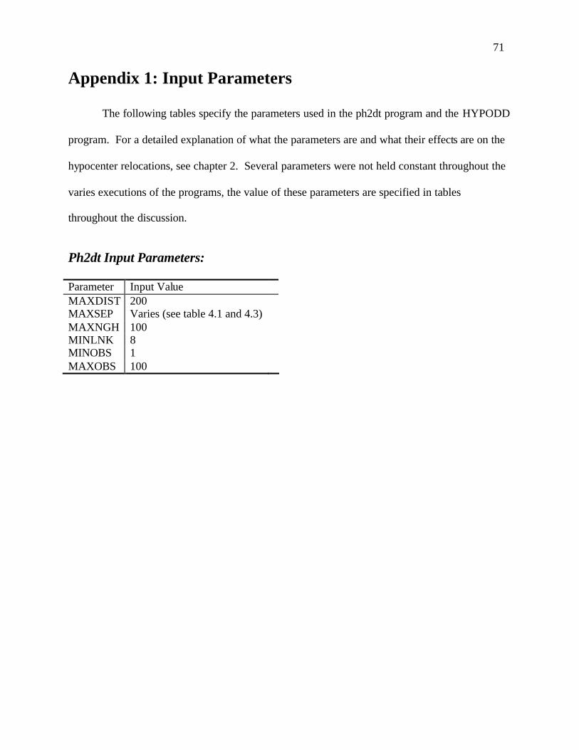
71

Appendix 1: Input Parameters The following tables specify the parameters used in the ph2dt program and the HYPODD

program. For a detailed explanation of what the parameters are and what their effects are on the

hypocenter relocations, see chapter 2. Several parameters were not held constant throughout the

varies executions of the programs, the value of these parameters are specified in tables

throughout the discussion.

Ph2dt Input Parameters: Parameter Input Value MAXDIST MAXSEP

200 Varies (see table 4.1 and 4.3)

MAXNGH 100 MINLNK 8 MINOBS 1 MAXOBS 100

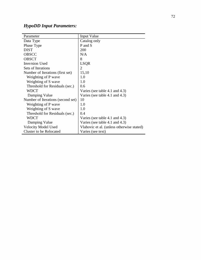
72

HypoDD Input Parameters: Parameter Input Value Data Type Catalog only Phase Type P and S DIST 200 OBSCC N/A OBSCT 8 Inversion Used LSQR Sets of Iterations 2 Number of Iterations (first set) 15,10 Weighting of P wave 1.0 Weighting of S wave 1.0 Threshold for Residuals (sec.) WDCT

0.6 Varies (see table 4.1 and 4.3)

Damping Value Varies (see table 4.1 and 4.3) Number of Iterations (second set) 10 Weighting of P wave Weighting of S wave

1.0 1.0

Threshold for Residuals (sec.) 0.4 WDCT Varies (see table 4.1 and 4.3) Damping Value Varies (see table 4.1 and 4.3) Velocity Model Used Vlahovic et al. (unless otherwise stated) Cluster to be Relocated Varies (see text)

73

Appendix 2: Velocity Models Two velocity models were used as input into HYPOELLIPSE (Lahr, 1980) or HYPODD

(Waldhauser, 2002). Unless otherwise specifically stated within the discussion, the Vlahovic et

al. (1998) velocity model was used. Below are both the Vlahovic et al. and Giles County

velocity models used as input.

Giles County Velocity Model: Layer P Wave

Velocity (km/s) Depth to the Top of Layer

Vp/Vs ratio (km/s)

1 5.63 0.0 1.64 2 6.05 5.7 1.72 3 6.53 14.7 1.70 4 8.18 50.7 1.71 **** when used in HYPODD, the Vp/Vs ratio is held constant at 1.72 km/s Vlahovic et al. Velocity Model: Layer P Wave

Velocity (km/s) Depth to the Top of Layer

Vp/Vs ratio (km/s)

1 6.05 0.0 1.74 2 6.24 5.7 1.73 3 6.34 10.0 1.73 4 6.43 14.7 1.72 5 6.52 20.0 1.72 6 8.00 45.0 1.72 ****when used in HYPODD, the Vp/Vs ratio is held constant at 1.73 km/s

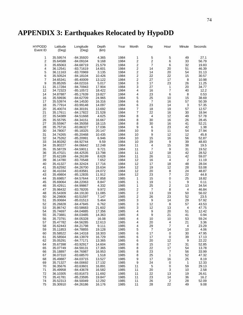
74

APPENDIX 3: Earthquakes Relocated by HypoDD

HYPODD Event ID

Latitude (Deg)

Longitude (Deg)

Depth (km)

Year Month Day Hour Minute Seconds

1 35.59574 -84.35920 4.365 1984 1 5 5 49 27.1 2 35.64588 -84.09104 9.168 1984 2 2 6 33 56.79 3 35.65063 -84.68719 21.579 1984 2 7 6 32 19.83 4 36.12541 -83.71619 14.601 1984 2 14 20 51 46.39 5 36.11163 -83.70969 3.135 1984 2 14 20 54 31.13 6 35.50524 -84.18104 10.426 1984 2 22 22 15 30.57 7 34.65341 -85.40009 13.122 1984 2 27 17 8 10.98 9 35.85265 -84.02316 5.017 1984 3 17 23 26 11.25

11 35.17284 -84.70943 17.904 1984 3 27 1 20 34.77 12 34.72323 -85.10572 18.422 1984 4 16 7 40 12.2 14 34.87887 -85.17639 19.827 1984 4 23 6 8 0.53 16 35.59936 -84.62709 24.965 1984 5 25 10 15 38.69 17 35.53974 -84.14530 16.316 1984 6 7 16 57 50.39 18 35.77914 -83.99148 14.097 1984 6 23 14 3 57.35 20 35.40074 -84.30191 13.692 1984 7 18 19 57 12.57 21 35.17611 -84.17822 21.528 1984 7 22 16 30 18.94 22 35.54389 -84.51668 4.625 1984 8 4 12 49 57.78 26 35.55795 -84.34151 16.667 1984 8 30 16 26 28.45 27 35.55967 -84.35058 18.115 1984 8 30 16 41 52.21 28 35.75716 -83.86327 17.036 1984 9 6 23 42 1.38 30 34.78007 -85.18325 20.147 1984 10 9 11 54 27.94 31 34.74265 -85.20468 10.435 1984 10 9 12 12 45.8 32 34.75262 -85.20991 6.946 1984 10 15 16 56 52.87 33 34.80282 -84.92744 9.59 1984 10 29 9 39 48.83 34 35.80227 -84.06642 12.248 1984 11 4 15 38 19.5 35 35.58729 -84.59011 9.721 1984 11 7 9 31 19.52 36 35.47021 -84.42535 13.798 1984 11 12 18 42 28.52 37 35.62189 -84.26199 8.628 1984 11 26 11 42 59.07 39 36.14780 -83.70548 7.652 1984 12 16 4 2 11.19 40 35.41327 -84.32424 17.716 1984 12 17 18 48 28.04 41 35.62592 -84.26700 15.634 1984 12 19 12 28 53.08 42 36.41034 -83.83581 24.072 1984 12 20 8 24 48.87 43 35.49804 -85.12835 11.912 1984 12 23 7 22 44.8 44 35.69857 -84.57644 17.858 1985 1 15 0 25 18.82 45 35.69064 -84.22063 8.847 1985 1 19 1 9 0.11 46 35.42911 -84.99867 4.332 1985 1 25 2 13 34.54 47 35.98432 -83.78205 9.972 1985 2 7 8 4 46.84 48 35.54309 -84.19130 11.085 1985 2 13 19 50 56.02 50 36.29806 -83.51597 7.147 1985 2 26 23 52 23.5 51 35.00684 -85.01513 5.464 1985 3 9 14 29 57.92 52 35.26828 -84.47845 6.762 1985 3 12 8 57 43.53 53 35.86742 -83.58683 21.602 1985 3 12 13 4 47.75 54 35.74697 -84.04885 17.356 1985 4 9 20 51 12.42 55 35.73881 -84.03485 14.363 1985 4 9 21 41 0.94 56 35.73791 -84.05328 16.08 1985 4 10 10 53 59.24 57 35.47782 -84.56285 12.613 1985 4 20 4 21 3.36 58 35.62443 -84.21798 9.111 1985 4 29 7 4 23.29 59 35.11853 -84.78855 19.128 1985 5 7 14 10 4.06 60 35.58522 -84.14318 18.303 1985 6 17 0 30 47.95 61 35.58564 -84.13979 16.729 1985 6 17 0 39 17.13 62 35.05291 -84.77171 13.365 1985 6 20 12 9 22.22 64 35.67398 -83.92917 14.604 1985 8 15 17 31 52.85 65 35.07749 -84.59131 17.365 1985 8 22 17 54 13.78 66 35.18897 -84.76987 16.953 1985 8 23 7 56 33.99 67 36.07310 -83.68570 1.518 1985 8 25 1 52 47.32 68 35.49887 -84.03715 13.527 1985 9 17 16 25 8.19 69 35.71327 -84.00692 17.132 1985 9 24 0 1 12.33 70 36.35676 -83.63601 16.891 1985 11 5 0 59 29.13 71 35.49958 -84.43678 16.582 1985 11 20 3 10 2.58 72 36.10305 -83.81673 11.692 1985 11 22 13 19 26.61 73 35.41781 -85.23595 19.847 1985 11 23 14 36 16.2 74 35.52313 -84.50049 12.292 1985 11 26 2 28 52.09 75 35.30910 -84.26186 16.176 1985 11 28 22 49 9.08

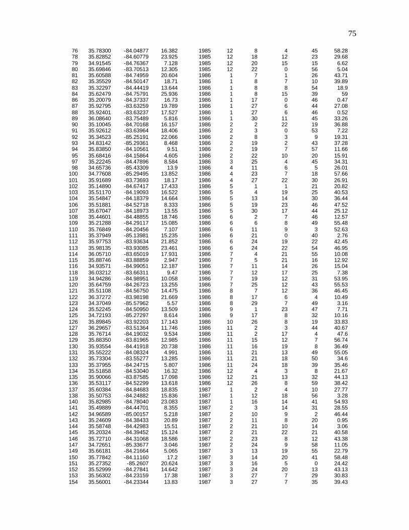
75

76 35.78300 -84.04877 16.382 1985 12 8 4 45 58.28 78 35.82852 -84.60779 23.925 1985 12 18 12 23 29.68 79 34.91545 -84.76367 7.128 1985 12 20 15 15 6.62 80 35.69846 -83.70513 12.305 1985 12 22 0 56 5.04 81 35.60588 -84.74959 20.604 1986 1 7 1 26 43.71 82 35.35529 -84.50147 18.71 1986 1 8 7 10 39.89 83 35.32297 -84.44419 13.644 1986 1 8 8 54 18.9 84 35.62479 -84.75791 25.936 1986 1 8 15 39 59 86 35.20079 -84.37337 16.73 1986 1 17 0 46 0.47 87 35.92795 -83.63259 19.789 1986 1 27 6 44 27.08 88 35.92401 -83.63237 17.527 1986 1 27 6 46 0.52 89 36.08640 -83.75489 5.816 1986 1 30 11 45 33.26 90 35.10045 -84.70168 16.157 1986 2 2 22 19 36.88 91 35.92612 -83.63964 18.406 1986 2 3 0 53 7.22 92 35.34523 -85.25191 22.066 1986 2 8 3 9 19.31 93 34.83142 -85.29361 8.468 1986 2 19 2 43 37.28 94 35.83850 -84.10561 9.51 1986 2 19 7 57 11.66 95 35.68416 -84.15864 4.605 1986 2 22 10 20 15.91 97 35.22245 -84.47896 8.584 1986 3 25 4 45 34.31 98 34.65736 -85.43309 13.9 1986 4 11 6 5 26.01

100 34.77608 -85.29495 13.852 1986 4 23 7 18 57.66 101 35.91689 -83.73693 18.17 1986 4 27 22 30 26.91 102 35.14890 -84.67417 17.433 1986 5 1 1 21 20.82 103 35.51170 -84.19093 16.522 1986 5 4 19 25 40.53 104 35.54847 -84.18379 14.664 1986 5 13 14 30 36.44 106 35.51881 -84.52718 8.333 1986 5 19 23 46 47.52 107 35.67047 -84.18973 13.55 1986 5 30 17 44 25.12 108 35.44601 -84.48855 18.746 1986 6 2 7 46 12.57 109 35.21288 -84.29117 15.085 1986 6 6 8 49 55.48 110 35.76849 -84.20456 7.107 1986 6 11 9 3 52.63 111 35.37949 -85.13981 15.235 1986 6 21 0 40 2.76 112 35.97753 -83.93634 21.852 1986 6 24 19 22 42.45 113 35.98135 -83.93085 23.461 1986 6 24 22 54 46.95 114 36.05710 -83.65019 17.931 1986 7 4 21 55 10.08 115 35.88746 -83.88859 2.947 1986 7 5 21 16 12.92 116 34.93571 -84.99051 12.187 1986 7 11 14 26 15.04 118 36.03212 -83.66311 9.47 1986 7 12 17 25 7.38 119 34.94286 -84.98951 10.058 1986 7 19 12 31 53.95 120 35.64759 -84.26723 13.255 1986 7 25 12 43 55.53 121 35.51108 -84.56750 14.475 1986 8 7 12 36 46.45 122 36.37272 -83.98198 21.669 1986 8 17 6 4 10.49 123 34.37049 -85.57962 5.57 1986 8 29 7 49 3.16 124 35.52245 -84.50950 13.509 1986 9 1 23 47 7.71 125 34.72193 -85.27297 8.614 1986 9 17 8 32 10.16 126 35.89845 -83.92203 17.143 1986 10 26 8 19 33.83 127 36.29657 -83.51364 11.746 1986 11 2 3 44 40.67 128 35.76714 -84.19032 9.534 1986 11 2 17 4 47.6 129 35.88350 -83.81965 12.985 1986 11 15 12 7 56.74 130 35.93554 -84.41918 20.738 1986 11 16 19 8 36.49 131 35.55222 -84.08324 4.991 1986 11 21 13 49 55.05 132 35.73304 -83.55277 13.285 1986 11 21 18 50 34.6 133 35.37955 -84.24715 5.807 1986 11 24 18 39 35.46 134 35.51858 -84.53040 16.32 1986 12 4 3 8 21.67 135 35.90066 -83.87585 17.098 1986 12 21 13 32 44.13 136 35.53117 -84.52299 13.618 1986 12 26 8 59 38.42 137 35.60384 -84.84683 18.835 1987 1 2 4 10 27.77 138 35.50753 -84.24882 15.836 1987 1 12 18 56 3.28 140 35.82985 -84.78040 23.083 1987 1 16 14 41 54.93 141 35.49889 -84.44701 8.355 1987 2 3 14 31 28.55 142 34.96589 -85.00157 5.218 1987 2 10 9 2 46.44 143 35.24609 -84.38433 20.89 1987 2 11 8 20 0.95 144 35.58748 -84.42983 15.51 1987 2 21 10 14 3.06 145 35.20324 -84.39452 15.124 1987 2 21 22 21 40.58 146 35.72710 -84.31068 18.586 1987 2 23 8 12 43.38 147 34.72651 -85.33677 3.046 1987 2 24 9 58 11.05 149 35.66181 -84.21664 5.065 1987 3 13 19 55 22.79 150 35.77842 -84.11160 17.2 1987 3 14 20 41 58.48 151 35.27352 -85.2607 20.624 1987 3 16 5 0 24.42 152 35.52999 -84.27841 14.642 1987 3 24 20 13 43.13 153 35.56302 -84.23159 17.38 1987 3 27 7 29 30.83 154 35.56001 -84.23344 13.83 1987 3 27 7 35 39.43

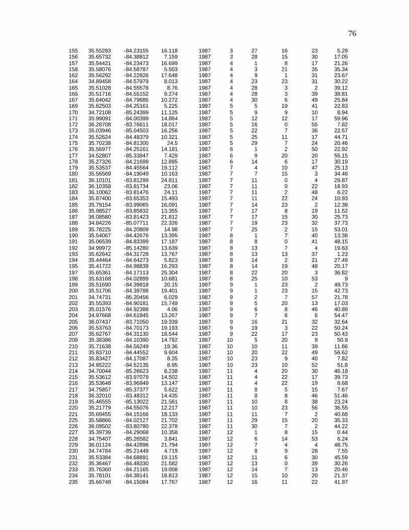
76

155 35.55283 -84.23155 16.118 1987 3 27 16 23 5.29 156 35.65732 -84.38812 7.159 1987 3 28 15 30 17.05 157 35.54421 -84.23473 16.699 1987 4 1 8 17 21.26 158 35.58076 -84.58787 5.503 1987 4 3 21 35 35.34 162 35.56292 -84.22826 17.648 1987 4 9 1 31 23.67 164 34.89458 -84.57979 8.013 1987 4 23 23 31 30.22 165 35.51028 -84.55578 8.76 1987 4 28 3 2 39.12 166 35.51716 -84.55152 9.274 1987 4 28 3 39 38.81 167 35.64042 -84.79685 10.272 1987 4 30 6 49 25.84 169 35.62503 -84.25161 5.225 1987 5 5 19 41 22.83 170 34.72108 -85.24399 11.125 1987 5 9 9 10 8.94 171 35.99091 -84.00399 14.864 1987 5 12 12 17 59.96 172 36.28708 -83.76611 18.017 1987 5 16 0 55 7.82 173 35.03946 -85.04503 16.256 1987 5 22 7 36 22.57 174 35.52624 -84.48379 10.321 1987 5 25 11 17 44.71 175 35.70238 -84.81300 24.5 1987 5 29 7 24 20.46 176 35.56977 -84.25161 14.181 1987 6 1 2 50 22.92 177 34.52807 -85.33847 7.429 1987 6 9 20 20 55.15 178 35.27326 -84.21699 12.895 1987 6 14 6 17 30.19 179 35.53537 -84.45564 19.112 1987 7 4 10 47 25.13 180 35.56569 -84.19049 10.163 1987 7 7 15 3 34.46 181 36.10101 -83.81299 24.811 1987 7 11 0 4 29.87 182 36.10358 -83.81734 23.06 1987 7 11 0 22 18.93 183 36.10062 -83.81476 24.11 1987 7 11 2 48 6.22 184 35.87400 -83.65353 15.493 1987 7 11 22 24 10.93 185 35.79154 -83.99065 16.091 1987 7 14 23 2 12.38 186 35.98527 -83.85832 13.355 1987 7 17 8 19 11.52 187 36.08580 -83.81423 21.812 1987 7 17 15 30 25.73 188 34.84226 -85.07711 22.326 1987 7 19 23 32 37.73 189 35.78225 -84.20809 14.98 1987 7 25 2 15 53.01 190 35.54067 -84.42676 13.395 1987 8 1 7 40 13.38 191 35.06539 -84.83399 17.187 1987 8 8 0 41 48.15 192 34.99972 -85.14280 13.639 1987 8 13 7 4 19.63 193 35.62642 -84.31728 13.767 1987 8 13 13 37 1.23 194 35.44464 -84.64273 5.823 1987 8 14 2 21 27.49 195 35.41722 -84.98839 16.293 1987 8 14 19 48 20.17 197 35.65361 -84.17113 25.304 1987 8 22 20 3 36.82 198 35.63168 -84.02899 10.681 1987 8 25 10 53 9 199 35.51690 -84.39818 20.15 1987 9 1 23 2 49.73 200 35.51706 -84.39788 19.401 1987 9 1 23 15 42.73 201 34.74731 -85.20456 6.029 1987 9 2 7 57 21.78 202 35.55393 -84.90181 15.749 1987 9 5 20 13 17.03 203 35.01576 -84.92388 4.06 1987 9 6 8 46 40.89 204 34.97668 -84.61845 13.267 1987 9 7 6 6 54.47 205 36.07437 -83.71050 19.339 1987 9 16 21 32 32.64 206 35.53763 -84.70173 19.193 1987 9 19 3 22 50.24 207 35.62767 -84.31130 18.544 1987 9 22 17 23 50.43 209 35.38386 -84.10390 14.792 1987 10 5 20 9 50.9 210 35.71638 -84.56249 19.36 1987 10 10 11 39 11.66 211 35.83710 -84.44552 9.604 1987 10 20 22 49 56.62 212 35.83427 -84.17087 8.35 1987 10 23 9 40 7.82 213 34.85222 -84.52135 8.95 1987 10 23 10 52 51.8 214 34.70044 -85.26623 8.238 1987 11 4 20 30 46.18 215 35.53612 -83.97079 14.502 1987 11 4 22 17 39.73 216 35.53648 -83.96849 13.147 1987 11 4 22 19 8.68 217 34.75857 -85.37377 5.622 1987 11 8 5 15 7.67 218 36.32010 -83.48312 14.435 1987 11 8 8 46 51.46 219 35.46555 -85.13022 21.561 1987 11 10 8 38 23.24 220 35.21779 -84.55076 12.217 1987 11 10 23 56 36.55 221 35.69455 -84.15166 18.133 1987 11 11 7 2 40.68 225 35.58866 -84.02127 21.702 1987 11 29 15 20 35.33 226 36.09502 -83.80780 22.378 1987 11 30 7 2 44.22 227 35.39739 -84.29068 10.358 1987 12 1 8 15 0.44 228 34.75407 -85.26582 3.841 1987 12 6 14 53 6.24 229 36.01124 -84.42896 21.794 1987 12 7 4 4 48.75 230 34.74784 -85.21449 4.719 1987 12 8 9 28 7.55 231 35.53384 -84.68891 19.115 1987 12 11 6 30 45.59 232 35.36467 -84.48330 21.582 1987 12 13 0 39 30.26 233 35.76360 -84.21165 19.008 1987 12 14 7 13 20.46 234 35.78101 -84.38141 18.813 1987 12 15 10 20 21.37 235 35.66748 -84.15084 17.767 1987 12 16 11 22 41.97

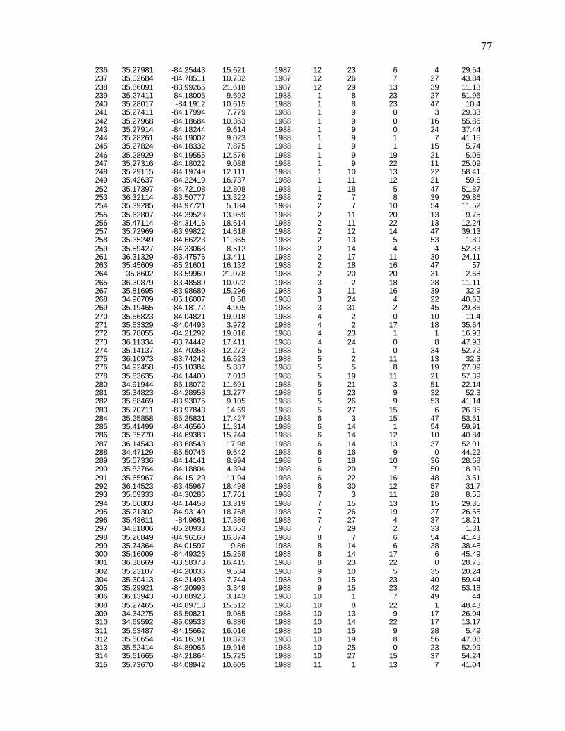
77

236 35.27981 -84.25443 15.621 1987 12 23 6 4 29.54 237 35.02684 -84.78511 10.732 1987 12 26 7 27 43.84 238 35.86091 -83.99265 21.618 1987 12 29 13 39 11.13 239 35.27411 -84.18005 9.692 1988 1 8 23 27 51.96 240 35.28017 -84.1912 10.615 1988 1 8 23 47 10.4 241 35.27411 -84.17994 7.779 1988 1 9 0 3 29.33 242 35.27968 -84.18684 10.363 1988 1 9 0 16 55.86 243 35.27914 -84.18244 9.614 1988 1 9 0 24 37.44 244 35.28261 -84.19002 9.023 1988 1 9 1 7 41.15 245 35.27824 -84.18332 7.875 1988 1 9 1 15 5.74 246 35.28929 -84.19555 12.576 1988 1 9 19 21 5.06 247 35.27316 -84.18022 9.088 1988 1 9 22 11 25.09 248 35.29115 -84.19749 12.111 1988 1 10 13 22 58.41 249 35.42637 -84.22419 16.737 1988 1 11 12 21 59.6 252 35.17397 -84.72108 12.808 1988 1 18 5 47 51.87 253 36.32114 -83.50777 13.322 1988 2 7 8 39 29.86 254 35.39285 -84.97721 5.184 1988 2 7 10 54 11.52 255 35.62807 -84.39523 13.959 1988 2 11 20 13 9.75 256 35.47114 -84.31416 18.614 1988 2 11 22 13 12.24 257 35.72969 -83.99822 14.618 1988 2 12 14 47 39.13 258 35.35249 -84.66223 11.365 1988 2 13 5 53 1.89 259 35.59427 -84.33068 8.512 1988 2 14 4 4 52.83 261 36.31329 -83.47576 13.411 1988 2 17 11 30 24.11 263 35.45609 -85.21601 16.132 1988 2 18 16 47 57 264 35.8602 -83.59960 21.078 1988 2 20 20 31 2.68 265 36.30879 -83.48589 10.022 1988 3 2 18 28 11.11 267 35.81695 -83.98680 15.296 1988 3 11 16 39 32.9 268 34.96709 -85.16007 8.58 1988 3 24 4 22 40.63 269 35.19465 -84.18172 4.905 1988 3 31 2 45 29.86 270 35.56823 -84.04821 19.018 1988 4 2 0 10 11.4 271 35.53329 -84.04493 3.972 1988 4 2 17 18 35.64 272 35.78055 -84.21292 19.016 1988 4 23 1 1 16.93 273 36.11334 -83.74442 17.411 1988 4 24 0 8 47.93 274 35.14137 -84.70358 12.272 1988 5 1 0 34 52.72 275 36.10973 -83.74242 16.623 1988 5 2 11 13 32.3 276 34.92458 -85.10384 5.887 1988 5 5 8 19 27.09 278 35.83635 -84.14400 7.013 1988 5 19 11 21 57.39 280 34.91944 -85.18072 11.691 1988 5 21 3 51 22.14 281 35.34823 -84.28958 13.277 1988 5 23 9 32 52.3 282 35.88469 -83.93075 9.105 1988 5 26 9 53 41.14 283 35.70711 -83.97843 14.69 1988 5 27 15 6 26.35 284 35.25858 -85.25831 17.427 1988 6 3 15 47 53.51 285 35.41499 -84.46560 11.314 1988 6 14 1 54 59.91 286 35.35770 -84.69383 15.744 1988 6 14 12 10 40.84 287 36.14543 -83.68543 17.98 1988 6 14 13 37 52.01 288 34.47129 -85.50746 9.642 1988 6 16 9 0 44.22 289 35.57336 -84.14141 8.994 1988 6 18 10 36 28.68 290 35.83764 -84.18804 4.394 1988 6 20 7 50 18.99 291 35.65967 -84.15129 11.94 1988 6 22 16 48 3.51 292 36.14523 -83.45967 18.498 1988 6 30 12 57 31.7 293 35.69333 -84.30286 17.761 1988 7 3 11 28 8.55 294 35.66803 -84.14453 13.319 1988 7 15 13 15 29.35 295 35.21302 -84.93140 18.768 1988 7 26 19 27 26.65 296 35.43611 -84.9661 17.386 1988 7 27 4 37 18.21 297 34.81806 -85.20933 13.653 1988 7 29 2 33 1.31 298 35.26849 -84.96160 16.874 1988 8 7 6 54 41.43 299 35.74364 -84.01597 9.86 1988 8 14 6 38 38.48 300 35.16009 -84.49326 15.258 1988 8 14 17 6 45.49 301 36.38669 -83.58373 16.415 1988 8 23 22 0 28.75 302 35.23107 -84.20036 9.534 1988 9 10 5 35 20.24 304 35.30413 -84.21493 7.744 1988 9 15 23 40 59.44 305 35.29921 -84.20993 3.349 1988 9 15 23 42 53.18 306 36.13943 -83.88923 3.143 1988 10 1 7 49 44 308 35.27465 -84.89718 15.512 1988 10 8 22 1 48.43 309 34.34275 -85.50821 9.085 1988 10 13 9 17 26.04 310 34.69592 -85.09533 6.386 1988 10 14 22 17 13.17 311 35.53487 -84.15662 16.016 1988 10 15 9 28 5.49 312 35.50654 -84.16191 10.873 1988 10 19 8 56 47.08 313 35.52414 -84.89065 19.916 1988 10 25 0 23 52.99 314 35.61665 -84.21864 15.725 1988 10 27 15 37 54.24 315 35.73670 -84.08942 10.605 1988 11 1 13 7 41.04

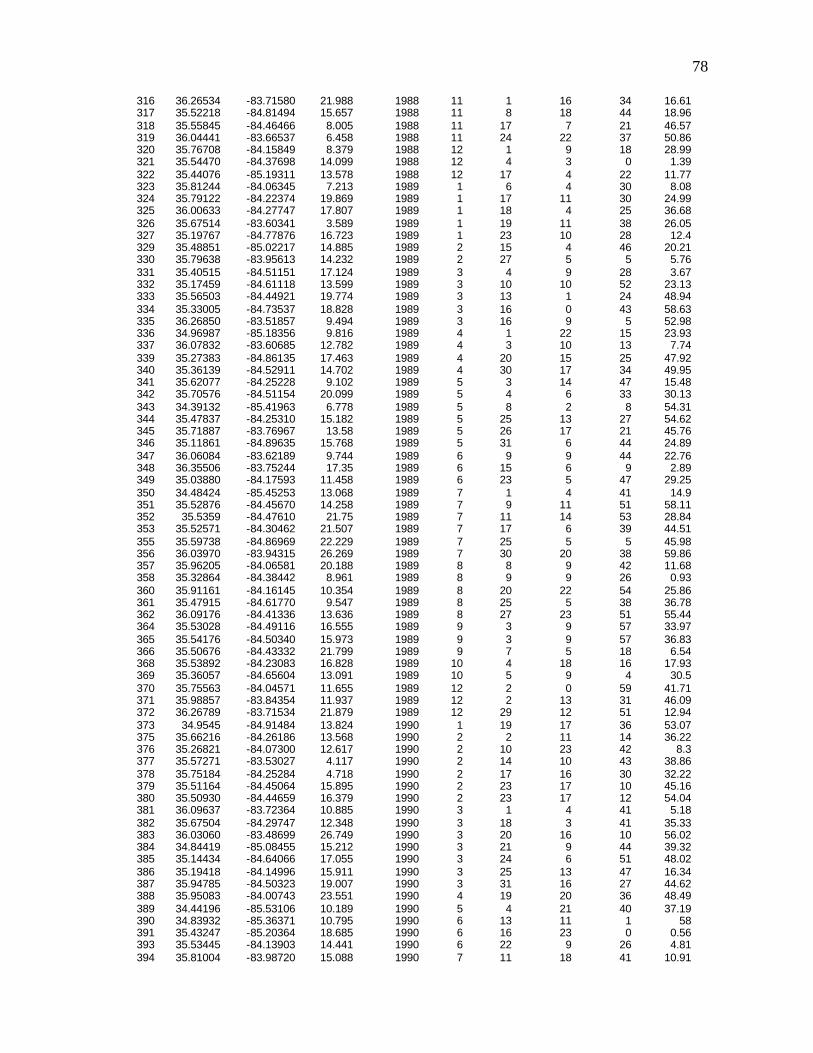
78

316 36.26534 -83.71580 21.988 1988 11 1 16 34 16.61 317 35.52218 -84.81494 15.657 1988 11 8 18 44 18.96 318 35.55845 -84.46466 8.005 1988 11 17 7 21 46.57 319 36.04441 -83.66537 6.458 1988 11 24 22 37 50.86 320 35.76708 -84.15849 8.379 1988 12 1 9 18 28.99 321 35.54470 -84.37698 14.099 1988 12 4 3 0 1.39 322 35.44076 -85.19311 13.578 1988 12 17 4 22 11.77 323 35.81244 -84.06345 7.213 1989 1 6 4 30 8.08 324 35.79122 -84.22374 19.869 1989 1 17 11 30 24.99 325 36.00633 -84.27747 17.807 1989 1 18 4 25 36.68 326 35.67514 -83.60341 3.589 1989 1 19 11 38 26.05 327 35.19767 -84.77876 16.723 1989 1 23 10 28 12.4 329 35.48851 -85.02217 14.885 1989 2 15 4 46 20.21 330 35.79638 -83.95613 14.232 1989 2 27 5 5 5.76 331 35.40515 -84.51151 17.124 1989 3 4 9 28 3.67 332 35.17459 -84.61118 13.599 1989 3 10 10 52 23.13 333 35.56503 -84.44921 19.774 1989 3 13 1 24 48.94 334 35.33005 -84.73537 18.828 1989 3 16 0 43 58.63 335 36.26850 -83.51857 9.494 1989 3 16 9 5 52.98 336 34.96987 -85.18356 9.816 1989 4 1 22 15 23.93 337 36.07832 -83.60685 12.782 1989 4 3 10 13 7.74 339 35.27383 -84.86135 17.463 1989 4 20 15 25 47.92 340 35.36139 -84.52911 14.702 1989 4 30 17 34 49.95 341 35.62077 -84.25228 9.102 1989 5 3 14 47 15.48 342 35.70576 -84.51154 20.099 1989 5 4 6 33 30.13 343 34.39132 -85.41963 6.778 1989 5 8 2 8 54.31 344 35.47837 -84.25310 15.182 1989 5 25 13 27 54.62 345 35.71887 -83.76967 13.58 1989 5 26 17 21 45.76 346 35.11861 -84.89635 15.768 1989 5 31 6 44 24.89 347 36.06084 -83.62189 9.744 1989 6 9 9 44 22.76 348 36.35506 -83.75244 17.35 1989 6 15 6 9 2.89 349 35.03880 -84.17593 11.458 1989 6 23 5 47 29.25 350 34.48424 -85.45253 13.068 1989 7 1 4 41 14.9 351 35.52876 -84.45670 14.258 1989 7 9 11 51 58.11 352 35.5359 -84.47610 21.75 1989 7 11 14 53 28.84 353 35.52571 -84.30462 21.507 1989 7 17 6 39 44.51 355 35.59738 -84.86969 22.229 1989 7 25 5 5 45.98 356 36.03970 -83.94315 26.269 1989 7 30 20 38 59.86 357 35.96205 -84.06581 20.188 1989 8 8 9 42 11.68 358 35.32864 -84.38442 8.961 1989 8 9 9 26 0.93 360 35.91161 -84.16145 10.354 1989 8 20 22 54 25.86 361 35.47915 -84.61770 9.547 1989 8 25 5 38 36.78 362 36.09176 -84.41336 13.636 1989 8 27 23 51 55.44 364 35.53028 -84.49116 16.555 1989 9 3 9 57 33.97 365 35.54176 -84.50340 15.973 1989 9 3 9 57 36.83 366 35.50676 -84.43332 21.799 1989 9 7 5 18 6.54 368 35.53892 -84.23083 16.828 1989 10 4 18 16 17.93 369 35.36057 -84.65604 13.091 1989 10 5 9 4 30.5 370 35.75563 -84.04571 11.655 1989 12 2 0 59 41.71 371 35.98857 -83.84354 11.937 1989 12 2 13 31 46.09 372 36.26789 -83.71534 21.879 1989 12 29 12 51 12.94 373 34.9545 -84.91484 13.824 1990 1 19 17 36 53.07 375 35.66216 -84.26186 13.568 1990 2 2 11 14 36.22 376 35.26821 -84.07300 12.617 1990 2 10 23 42 8.3 377 35.57271 -83.53027 4.117 1990 2 14 10 43 38.86 378 35.75184 -84.25284 4.718 1990 2 17 16 30 32.22 379 35.51164 -84.45064 15.895 1990 2 23 17 10 45.16 380 35.50930 -84.44659 16.379 1990 2 23 17 12 54.04 381 36.09637 -83.72364 10.885 1990 3 1 4 41 5.18 382 35.67504 -84.29747 12.348 1990 3 18 3 41 35.33 383 36.03060 -83.48699 26.749 1990 3 20 16 10 56.02 384 34.84419 -85.08455 15.212 1990 3 21 9 44 39.32 385 35.14434 -84.64066 17.055 1990 3 24 6 51 48.02 386 35.19418 -84.14996 15.911 1990 3 25 13 47 16.34 387 35.94785 -84.50323 19.007 1990 3 31 16 27 44.62 388 35.95083 -84.00743 23.551 1990 4 19 20 36 48.49 389 34.44196 -85.53106 10.189 1990 5 4 21 40 37.19 390 34.83932 -85.36371 10.795 1990 6 13 11 1 58 391 35.43247 -85.20364 18.685 1990 6 16 23 0 0.56 393 35.53445 -84.13903 14.441 1990 6 22 9 26 4.81 394 35.81004 -83.98720 15.088 1990 7 11 18 41 10.91

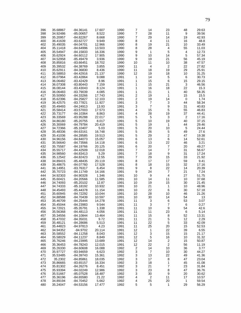
79

396 35.68867 -84.36141 17.607 1990 7 14 23 48 29.63 398 34.92486 -85.00657 8.522 1990 7 28 11 9 39.56 399 35.20957 -84.82267 8.668 1990 7 29 14 19 42.93 400 36.41639 -83.62727 9.949 1990 8 4 11 16 48.8 402 35.49035 -84.04701 12.966 1990 8 19 21 10 33.49 404 35.11418 -84.64996 13.503 1990 8 28 4 55 11.03 405 35.54947 -84.15833 16.336 1990 9 1 5 4 12.73 406 35.62924 -84.60112 17.905 1990 9 10 14 5 57.34 407 34.52958 -85.49479 3.936 1990 9 19 21 56 45.19 408 35.85816 -83.66451 18.702 1990 10 11 10 38 47.57 409 35.39532 -84.38769 3.855 1990 11 4 2 22 27.82 410 35.62911 -84.36830 8.436 1990 11 18 19 29 25.91 411 35.58853 -84.42916 21.137 1990 12 19 18 10 31.25 412 36.07964 -83.42864 9.088 1991 1 14 5 6 30.73 413 36.06482 -83.42429 8.96 1991 1 15 6 15 29.15 414 36.07308 -83.80443 7.159 1991 1 15 21 3 46.56 415 36.08144 -83.43043 8.124 1991 1 16 18 22 15.3 416 36.06483 -83.79039 4.085 1991 1 21 1 40 58.35 417 35.50950 -84.33266 17.743 1991 2 19 1 15 15.5 418 35.62396 -84.25827 12.103 1991 2 19 14 0 1.74 419 36.42575 -83.77821 11.927 1991 3 7 3 44 58.34 420 35.49493 -84.24913 13.93 1991 3 7 9 31 40.83 421 35.58414 -83.57003 17.573 1991 4 15 5 55 46.83 422 35.73177 -84.10364 8.863 1991 4 28 19 37 44.41 423 36.33569 -83.95288 22.017 1991 5 5 3 2 17.16 425 34.86180 -85.20755 8.017 1991 5 10 19 40 37.15 426 35.30069 -84.79784 20.419 1991 5 19 1 44 29.46 427 34.72366 -85.10407 5.03 1991 5 20 10 5 24.44 428 35.48336 -84.63161 16.748 1991 5 26 5 49 27.6 429 35.41036 -84.28585 19.513 1991 5 29 2 47 19.38 430 34.96156 -84.84073 15.057 1991 6 13 6 14 52.61 431 35.56640 -84.73566 14.118 1991 6 13 22 46 3.21 432 35.75587 -84.19766 20.125 1991 6 20 7 20 49.27 434 35.55717 -84.42509 12.018 1991 7 14 7 31 56.67 435 34.98560 -84.83413 5.29 1991 7 18 9 31 17.24 436 35.12542 -84.82423 12.55 1991 7 29 15 33 21.92 438 34.89415 -85.48435 20.119 1991 8 17 17 59 9.41 439 35.48675 -84.07760 17.528 1991 8 18 15 32 17.16 441 36.14951 -83.76317 6.454 1991 9 8 22 14 20.39 442 35.70723 -84.11749 14.166 1991 9 24 7 21 7.24 444 34.92303 -84.90328 1.346 1991 10 9 4 27 51.75 445 35.60421 -84.20566 11.585 1991 10 14 11 10 37.68 446 34.74093 -85.20102 12.87 1991 10 19 15 30 21.45 447 34.74333 -85.18192 10.932 1991 10 21 1 10 48.96 448 34.45493 -85.44378 11.154 1991 10 22 6 30 57.18 451 35.60945 -84.72292 10.044 1991 10 28 10 46 21.26 452 34.88588 -84.70439 10.597 1991 10 30 14 54 13 453 35.46709 -84.25444 14.278 1991 11 3 6 53 3.07 454 35.45044 -84.23983 9.544 1991 11 3 7 6 0.27 455 34.72021 -85.35791 1.338 1991 11 10 9 54 42.6 456 35.56368 -84.48113 4.056 1991 11 11 23 6 5.14 457 35.34556 -84.10844 13.464 1991 11 15 8 52 13.31 458 35.47032 -84.35031 9.72 1991 11 21 5 12 2.29 459 35.48121 -84.28686 5.513 1991 11 22 5 33 42.09 461 35.44823 -84.97813 4.23 1991 11 25 20 15 52.53 462 34.94352 -84.9702 20.114 1991 12 1 22 39 6.55 463 35.58552 -84.11258 8.043 1991 12 3 15 15 21.17 464 35.58029 -84.11237 8.849 1991 12 5 16 10 31.32 465 35.76246 -84.23995 13.689 1991 12 14 2 15 50.87 466 35.36453 -84.78243 12.015 1991 12 22 2 56 11.19 469 35.26330 -84.60608 16.088 1992 2 14 10 36 3.77 470 35.97727 -83.94659 6.623 1992 3 7 10 30 44.27 471 35.53485 -84.39743 15.361 1992 3 13 22 49 41.36 472 35.2302 -84.85861 18.035 1992 3 17 8 47 23.04 473 35.86665 -83.65157 16.334 1992 3 18 1 45 41.08 474 35.81302 -84.26276 8.451 1992 3 21 7 23 31.84 475 35.93394 -84.02249 12.986 1992 3 23 8 47 36.76 476 35.51667 -85.07528 18.487 1992 3 30 9 20 30.62 477 35.36196 -84.65580 21.22 1992 4 2 11 17 10.57 478 34.89194 -84.70452 5.662 1992 4 25 20 1 59.54 480 35.24047 -84.53156 17.477 1992 5 5 1 29 56.29

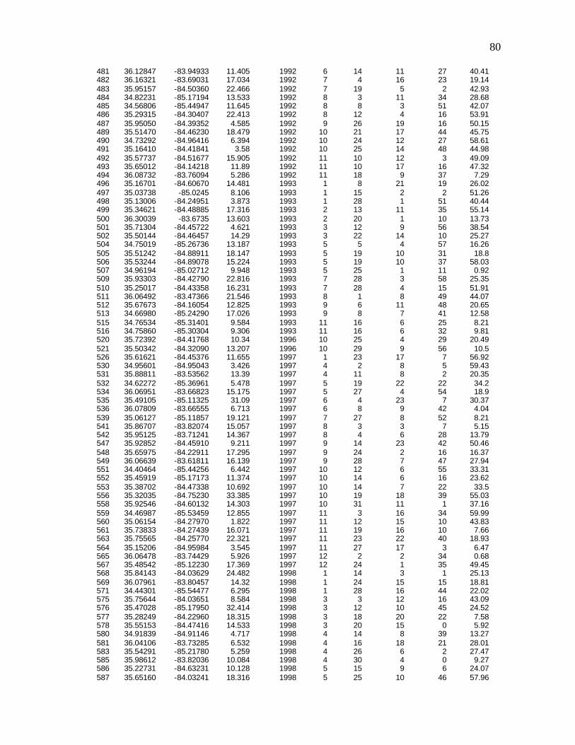
80

481 36.12847 -83.94933 11.405 1992 6 14 11 27 40.41 482 36.16321 -83.69031 17.034 1992 7 4 16 23 19.14 483 35.95157 -84.50360 22.466 1992 7 19 5 2 42.93 484 34.82231 -85.17194 13.533 1992 8 3 11 34 28.68 485 34.56806 -85.44947 11.645 1992 8 8 3 51 42.07 486 35.29315 -84.30407 22.413 1992 8 12 4 16 53.91 487 35.95050 -84.39352 4.585 1992 9 26 19 16 50.15 489 35.51470 -84.46230 18.479 1992 10 21 17 44 45.75 490 34.73292 -84.96416 6.394 1992 10 24 12 27 58.61 491 35.16410 -84.41841 3.58 1992 10 25 14 48 44.98 492 35.57737 -84.51677 15.905 1992 11 10 12 3 49.09 493 35.65012 -84.14218 11.89 1992 11 10 17 16 47.32 494 36.08732 -83.76094 5.286 1992 11 18 9 37 7.29 496 35.16701 -84.60670 14.481 1993 1 8 21 19 26.02 497 35.03738 -85.0245 8.106 1993 1 15 2 2 51.26 498 35.13006 -84.24951 3.873 1993 1 28 1 51 40.44 499 35.34621 -84.48885 17.316 1993 2 13 11 35 55.14 500 36.30039 -83.6735 13.603 1993 2 20 1 10 13.73 501 35.71304 -84.45722 4.621 1993 3 12 9 56 38.54 502 35.50144 -84.46457 14.29 1993 3 22 14 10 25.27 504 34.75019 -85.26736 13.187 1993 5 5 4 57 16.26 505 35.51242 -84.88911 18.147 1993 5 19 10 31 18.8 506 35.53244 -84.89078 15.224 1993 5 19 10 37 58.03 507 34.96194 -85.02712 9.948 1993 5 25 1 11 0.92 509 35.93303 -84.42790 22.816 1993 7 28 3 58 25.35 510 35.25017 -84.43358 16.231 1993 7 28 4 15 51.91 511 36.06492 -83.47366 21.546 1993 8 1 8 49 44.07 512 35.67673 -84.16054 12.825 1993 9 6 11 48 20.65 513 34.66980 -85.24290 17.026 1993 9 8 7 41 12.58 515 34.76534 -85.31401 9.584 1993 11 16 6 25 8.21 516 34.75860 -85.30304 9.306 1993 11 16 6 32 9.81 520 35.72392 -84.41768 10.34 1996 10 25 4 29 20.49 521 35.50342 -84.32090 13.207 1996 10 29 9 56 10.5 526 35.61621 -84.45376 11.655 1997 1 23 17 7 56.92 530 34.95601 -84.95043 3.426 1997 4 2 8 5 59.43 531 35.88811 -83.53562 13.39 1997 4 11 8 2 20.35 532 34.62272 -85.36961 5.478 1997 5 19 22 22 34.2 534 36.06951 -83.66823 15.175 1997 5 27 4 54 18.9 535 35.49105 -85.11325 31.09 1997 6 4 23 7 30.37 536 36.07809 -83.66555 6.713 1997 6 8 9 42 4.04 539 35.06127 -85.11857 19.121 1997 7 27 8 52 8.21 541 35.86707 -83.82074 15.057 1997 8 3 3 7 5.15 542 35.95125 -83.71241 14.367 1997 8 4 6 28 13.79 547 35.92852 -84.45910 9.211 1997 9 14 23 42 50.46 548 35.65975 -84.22911 17.295 1997 9 24 2 16 16.37 549 36.06639 -83.61811 16.139 1997 9 28 7 47 27.94 551 34.40464 -85.44256 6.442 1997 10 12 6 55 33.31 552 35.45919 -85.17173 11.374 1997 10 14 6 16 23.62 553 35.38702 -84.47338 10.692 1997 10 14 7 22 33.5 556 35.32035 -84.75230 33.385 1997 10 19 18 39 55.03 558 35.92546 -84.60132 14.303 1997 10 31 11 1 37.16 559 34.46987 -85.53459 12.855 1997 11 3 16 34 59.99 560 35.06154 -84.27970 1.822 1997 11 12 15 10 43.83 561 35.73833 -84.27439 16.071 1997 11 19 16 10 7.66 563 35.75565 -84.25770 22.321 1997 11 23 22 40 18.93 564 35.15206 -84.95984 3.545 1997 11 27 17 3 6.47 565 36.06478 -83.74429 5.926 1997 12 2 2 34 0.68 567 35.48542 -85.12230 17.369 1997 12 24 1 35 49.45 568 35.84143 -84.03629 24.482 1998 1 14 3 1 25.13 569 36.07961 -83.80457 14.32 1998 1 24 15 15 18.81 571 34.44301 -85.54477 6.295 1998 1 28 16 44 22.02 575 35.75644 -84.03651 8.584 1998 3 3 12 16 43.09 576 35.47028 -85.17950 32.414 1998 3 12 10 45 24.52 577 35.28249 -84.22960 18.315 1998 3 18 20 22 7.58 578 35.55153 -84.47416 14.533 1998 3 20 15 0 5.92 580 34.91839 -84.91146 4.717 1998 4 14 8 39 13.27 581 36.04106 -83.73285 6.532 1998 4 16 18 21 28.01 583 35.54291 -85.21780 5.259 1998 4 26 6 2 27.47 585 35.98612 -83.82036 10.084 1998 4 30 4 0 9.27 586 35.22731 -84.63231 10.128 1998 5 15 9 6 24.07 587 35.65160 -84.03241 18.316 1998 5 25 10 46 57.96

81

589 36.12068 -83.75390 17.592 1998 6 17 4 1 2.01 590 35.95457 -84.38572 13.464 1998 6 17 8 0 23.74 591 35.93228 -84.40333 9.088 1998 6 17 18 7 45.99 592 34.7084 -85.20179 1.889 1998 6 18 5 9 59.36 594 35.56763 -85.10495 22.829 1998 7 3 13 6 49.45 595 35.53721 -84.53459 7.642 1998 7 4 11 24 18.67 597 35.77852 -84.23755 9.813 1998 8 8 6 54 33.84 598 35.77816 -84.22938 4.266 1998 8 8 7 53 52.16 602 34.86520 -85.19493 4.027 1998 9 5 7 16 34.69 603 35.2158 -84.26791 12.879 1998 9 13 11 22 43.24 604 36.12149 -83.68126 9.238 1998 9 13 15 47 8.5 608 35.40911 -84.33997 6.778 1998 10 20 16 30 10.74 610 35.40369 -85.20666 15.776 1998 11 13 22 28 48.62 611 34.60581 -85.45823 1.567 1998 12 5 5 46 58.8 614 35.56806 -84.60655 9.368 1999 1 16 22 49 28.71 619 36.02876 -83.66320 8.111 1999 3 13 6 57 56.78 620 35.49695 -84.14817 13.191 1999 4 2 11 3 24.72 621 35.49605 -84.14326 14.529 1999 4 2 11 34 42.36 623 34.99689 -84.81431 11.388 1999 4 12 6 42 40.04 624 35.88823 -84.01088 18.516 1999 4 15 1 11 56.82 625 35.64172 -84.32854 15.741 1999 4 17 0 31 0.05 626 35.55819 -84.44640 11.137 1999 4 24 10 43 51.86 627 36.11687 -83.68983 7.046 1999 4 27 1 6 51.96 628 35.30636 -84.956 9.415 1999 5 17 17 29 32.94 629 35.30754 -84.95133 5.726 1999 5 18 2 34 15.69 630 35.30664 -84.94978 8.251 1999 5 18 2 45 20.85 631 35.59954 -84.71144 23.055 1999 5 22 8 55 36.57 632 35.72701 -83.89456 22.671 1999 5 22 15 20 54.11 633 35.75147 -83.95476 16.013 1999 5 27 11 21 0.3 636 36.10293 -83.68581 0.094 1999 5 30 3 41 56.67 639 35.33840 -85.07542 9.864 1999 6 28 1 53 4.01 640 35.63502 -84.30471 27.336 1999 7 6 6 21 4.57 642 36.06804 -83.66218 4.429 1999 7 16 1 54 22.45 647 35.36282 -84.23611 25.602 1999 9 17 12 24 14.35 649 35.61602 -84.22115 15.918 1999 10 19 9 38 14.99 652 35.44782 -84.61825 11.617 1999 11 17 3 31 22.81 654 35.61778 -84.09335 8.995 1999 11 28 9 30 31.17 656 35.03312 -84.85881 8.133 1999 12 8 21 18 41.86 658 35.35742 -84.76864 22.913 2000 1 3 21 24 59.9 662 35.65631 -84.31710 4.337 2000 3 4 19 8 24.96 663 35.32379 -85.10728 12.1 2000 3 12 6 20 23.72 664 34.68782 -85.37566 11.736 2000 3 20 10 0 50.62 665 34.69636 -85.38698 7.906 2000 3 20 19 36 50.4 666 35.42440 -85.34932 12.399 2000 3 24 19 45 26.81 667 35.47575 -85.08097 20.79 2000 4 3 23 39 34.26 668 35.46373 -84.17242 17.16 2000 4 10 12 48 15.39 669 35.67113 -84.31596 7.791 2000 4 12 3 54 5.77 670 36.25286 -83.93386 11.576 2000 4 16 2 38 44.72 671 35.53052 -84.77809 13.247 2000 4 25 3 0 19.43 672 35.90247 -84.57987 25.858 2000 5 3 12 48 31.21 674 35.17504 -84.88263 3.925 2000 5 15 15 5 34.31 676 35.55076 -84.16821 9.814 2000 6 4 5 6 47.57 678 35.20297 -84.29849 15.242 2000 7 2 14 20 21.99 680 35.80457 -83.95900 13.453 2000 7 8 21 41 2.08 681 35.88677 -83.80862 12.98 2000 7 11 14 59 47.61 682 35.48564 -85.15323 20.512 2000 7 11 17 44 26.83 683 35.54238 -85.16744 16.18 2000 7 12 6 27 5.32 684 35.31910 -85.14016 16.934 2000 7 21 15 35 12.03 685 35.66848 -84.25034 16.355 2000 7 28 20 16 39.4 689 35.92153 -84.62807 19.693 2000 8 23 8 12 43.06 696 35.62277 -84.06882 7.08 2000 10 19 6 39 27.01 697 35.72996 -84.21058 20.2 2000 10 21 18 36 0.48 698 35.56171 -84.75045 9.75 2000 10 23 7 57 30.51 700 35.49536 -85.04865 16.388 2000 11 9 15 13 55.51 701 35.53067 -84.48425 13.215 2000 11 18 16 22 9.71 702 35.51542 -84.47334 14.117 2000 11 18 17 8 1.99 704 35.45169 -84.62983 34.748 2000 12 10 17 51 50.53 714 35.76654 -83.99796 7.31 2001 2 18 19 17 4.26 715 35.16201 -84.80193 11.404 2001 2 20 7 8 36.28 718 35.69314 -84.34763 23.11 2001 2 27 16 46 26.88 719 35.52412 -84.83973 14.058 2001 3 7 17 12 24.05

82

723 35.52275 -84.49177 15.434 2001 3 30 22 1 12.58 724 35.63378 -84.30080 6.93 2001 4 5 23 20 33.22 733 36.03911 -83.83907 4.582 2001 5 17 6 43 48.5 734 35.82045 -83.95873 3.236 2001 5 21 2 36 6 748 35.21674 -84.90629 23.73 2001 10 29 21 40 41.82 755 35.69219 -84.06832 20.003 2001 12 5 13 7 39.44 760 35.68838 -84.55464 8.205 2002 2 17 7 0 43.57 762 36.01712 -83.84101 8.536 2002 2 25 1 53 16.06 766 34.67133 -84.95742 9.995 2002 4 6 20 49 51.79 769 35.53726 -84.07339 19.876 2002 5 15 6 34 50.34 770 35.62119 -84.21688 18.991 2002 5 16 7 5 30.18 773 35.94528 -83.83785 13.015 2002 7 24 11 31 21.69 774 35.88061 -84.02473 21.603 2002 8 4 1 56 54.05 775 35.65113 -84.85143 4.271 2002 8 16 13 40 12.35 777 35.64809 -84.84318 5.621 2002 8 27 14 7 35.57 780 35.37647 -84.36163 15.975 2002 10 2 21 55 19.66