IZA DP No. 808

Remittances and Inequality:A Dynamic Migration Model

Frédéric DocquierHillel Rapoport

DI

SC

US

SI

ON

PA

PE

R S

ER

IE

S

Forschungsinstitutzur Zukunft der ArbeitInstitute for the Studyof Labor

June 2003

Remittances and Inequality: A Dynamic Migration Model

Frédéric Docquier CADRE, University of Lille 2

and IZA Bonn

Hillel Rapoport CREDPR, Stanford University, CADRE and Bar-Ilan University

Discussion Paper No. 808 June 2003

IZA

P.O. Box 7240 D-53072 Bonn

Germany

Tel.: +49-228-3894-0 Fax: +49-228-3894-210

Email: iza@iza.org

This Discussion Paper is issued within the framework of IZA’s research area Mobility and Flexibility of Labor. Any opinions expressed here are those of the author(s) and not those of the institute. Research disseminated by IZA may include views on policy, but the institute itself takes no institutional policy positions. The Institute for the Study of Labor (IZA) in Bonn is a local and virtual international research center and a place of communication between science, politics and business. IZA is an independent, nonprofit limited liability company (Gesellschaft mit beschränkter Haftung) supported by Deutsche Post World Net. The center is associated with the University of Bonn and offers a stimulating research environment through its research networks, research support, and visitors and doctoral programs. IZA engages in (i) original and internationally competitive research in all fields of labor economics, (ii) development of policy concepts, and (iii) dissemination of research results and concepts to the interested public. The current research program deals with (1) mobility and flexibility of labor, (2) internationalization of labor markets, (3) welfare state and labor market, (4) labor markets in transition countries, (5) the future of labor, (6) evaluation of labor market policies and projects and (7) general labor economics. IZA Discussion Papers often represent preliminary work and are circulated to encourage discussion. Citation of such a paper should account for its provisional character. A revised version may be available on the IZA website (www.iza.org) or directly from the author.

IZA Discussion Paper No. 808 June 2003

ABSTRACT

Remittances and Inequality: A Dynamic Migration Model

We develop a model of the interdependencies between migration, remittances and inequality, and investigate how migration and subsequent remittances affect inter-household inequality in the origin communities. An important feature of our model is that we take into account the impact of migration on the local (rural) labor market. Migration is shown to decrease wealth inequality but may generate higher income inequality. Moreover, the short-run and long-run impacts of migration on income inequality may also be of opposite signs, suggesting that the dynamic relationship between migration and inequality may well be characterized by an inverse U-shaped pattern. This is consistent with the findings of the empirical literature on remittances and inequality, but offers a different interpretation, with no need to endogenize migration costs through the role of migrant networks. JEL Classification: O11, O15, J61, D31 Keywords: migration, remittances, inequality Corresponding author: Frédéric Docquier CADRE University of Lille 2 1 Place Déliot 59084 Lille France Email: f.docquier@skynet.be

1 Introduction

The economic analysis of migrants’ remittances has traditionally been divided

into two parts.1 At a micro level, an impressive body of work endeavors to un-

derstand remittance behavior and motivations to remit. Remittances are now

well recognized as part of an informal familial arrangement that goes well beyond

altruism, with bene…ts in the realms of mutual insurance, consumption smooth-

ing, and alleviation of liquidity constraints.2 At a macro level, the short-run

e¤ects of remittances have been analyzed mainly within the framework of trade-

theoretic models (e.g., Djajic, 1986, McCormick and Wahba, 2000); at the same

time, a series of recent studies have demonstrated the growth potential of migra-

tion in a context of capital market imperfections, with remittances and savings

accumulated abroad allowing households at the middle-to-bottom end of the

wealth distribution to accumulate productive assets (e.g., Lucas, 1987, Rozelle

et al., 1999) and access to self-employment and entrepreneurship.3 Another

strand of the literature has been concerned with the impact of international mi-

gration on income inequality at origin. For example, Adams (1989) found that

international migration tends to worsen economic inequality in rural Egypt,

while the same author found a neutral e¤ect in rural Pakistan (Adams, 1992).

In the case of rural Mexico, Taylor and Wyatt (1996) showed that remittances

are distributed almost evenly across income groups, hence inducing a direct

equalizing e¤ect in terms of economic inequality. In addition, they also showed

1For a survey on the economics of migrants’ remittances, see Rapoport and Docquier(2003).

2 In particular, the ’investment hypothesis’, according to which remittances must be seenas repayments of familial loans aimed at …nancing investments in education and/or migration,has recently received strong empirical support (Lucas and Stark, 1985, Poirine, 1997, Cox etal., 1998, Ilahi and Jafarey, 1999).

3For recent case-studies on return migration and access to entrepreneurship, see Ilahi (1999)on Pakistan, McCormick and Wahba (2001) on Egypt, Woodru¤ and Zenteno (2001) onMexico, Mesnard and Ravallion (2001) on Tunisia, or Dustmann and Kirchkamp (2002) onTurkey.

2

that remittances have the highest shadow value for households at the middle-

to-low-end of the income distribution; for such households indeed, remittances

allow for accessing to productive assets (land) and/or complementary inputs; a

second equalizing e¤ect is thereby obtained. This suggests that the impact of

remittances on rural development depends not only on the initial distribution

of wealth in the origin community, but also on a host of factors a¤ecting their

shadow value (e.g., degree of liquidity of land rights, costs of complementary

inputs, availability of local labor, etc.). In their study of remittances to a small

coastal city of Nicaragua, Barham and Boucher (1998) also …nd that remittances

apparently decrease income inequality. However, using di¤erent no-migration

counterfactuals to control for self-selection into migration and local labor-force

participation, they show that in reality remittances increase income inequal-

ity; this is explained by the fact that the potential home earnings of erstwhile

migrants have a more equalizing e¤ect on income distribution than remittances.

The impact of remittances in terms of economic inequality, however, needs

not be monotonic. Stark, Taylor and Yitzhaki (1986 and 1988) emphasized

that remittances tend to reduce economic inequality at origin, but suggested

that the dynamics of migration and remittances may be represented by an in-

verse U-shaped relationship: in the presence of liquidity constraints and initially

high migration costs, high-income groups only can access higher income oppor-

tunities abroad and, consequently, remittances tend to increase inter-household

inequality; as the number of migrants increases, migration costs tend to de-

crease thanks to the role of migrants’ networks, thus making migration a¤ord-

able to low-income households so that ultimately economic inequality at origin

decreases. Their analysis was based on the decomposition of a Gini index of

household income per income sources, taking account of the correlations be-

3

tween di¤erent income components. The method was applied to household data

from two Mexican villages, one with a relatively recent Mexico-to-US migration

experience, and one with a longer migration history. The distributional impact

of remittances was shown to depend on the village’s migration history, which

implicitly captures the magnitude of migration costs.4 They showed that income

dispersion was decreased in both villages once migrants’ remittances were taken

into account, but more so in the village characterized by a longer migration

tradition. With a similar approach applied to Yugoslavia, Milanovic (1987) also

tested for the possibility of such a ”trickle-down” e¤ect. Using inter-temporal

data from the 1973, 1978 and 1983 Yugoslavian household surveys, Milanovic

found no empirical support for this hypothesis. Indeed, his results were that

remittances tend to raise income inequality, although their e¤ects di¤er over the

periods and social categories considered (it was mainly for agricultural house-

holds that such an inequality-enhancing e¤ect over time was found). Finally,

Taylor’s (1992) longitudinal study of a Mexican village shows that remittances

may well have an inequality-enhancing e¤ect in the short-run and yet contribute

to decrease income inequality in the long-run in allowing poor rural households

to transform remittance income into productive assets.

On the whole, cross-sectional as well as panel data studies of remittances and

inequality do not o¤er a decisive conclusion as to whether international migra-

tion increases or decreases economic inequality at origin. This may be attributed

to the diversity of the environments studied in terms of initial inequality, as well

as to di¤erences in the empirical methodologies implemented: static v. dynamic

4Treating migration costs as exogenous may be adapted to situations where migration costsmainly include transportation and border crossing expenditures, but is clearly unsatisfactorywhen information costs (e.g., search process for a destination, and a job at destination) aresubstantial; in this case, it is well known that migration costs tend to decrease as the size ofthe relevant network at destination increases. Such network e¤ects have …rst been recognizedin the sociological literature (e.g, Massey et al., 1994) and, more recently, in the economicliterature (Carrington et al., 1996, Munshi, 2003).

4

studies with or without endogenous migration costs, and whether remittances

must be treated as a substitute for domestic earnings, in which case the e¤ect

of migration on domestic income sources must also be taken into account. In

this paper we propose a dynamic framework that goes part of the way towards

reconciling the con‡icting results of the empirical literature. We …rst qualify

di¤erent regimes of low, middle and high initial inequality which condition the

dynamics of migration and inequality in the migrants’ origin communities. A

notable feature of the model is that we take into account the impact of migra-

tion on local (rural) wages, and investigate whether domestic wages responses

reinforce or o¤set the inequality-e¤ect of remittances per se. Finally, while we

treat migration costs as exogenous, we also explore the e¤ect of decreasing mi-

gration costs, possibly through migration network e¤ects. Recall that the main

implication of the network hypothesis is that the impact of remittances on eco-

nomic inequality is likely to vary over time since migration may be viewed as a

di¤usion process with decreasing information costs. We complement this view

in showing that the same results may be obtained in a dynamic framework with

exogenous (i.e., constant) migration costs.

The remainder of this paper is organized as follows. In Section 2 we build a

model with two classes of agents characterized by di¤erent wealth (e.g., land)

endowments; this determines the household members’ labor productivity, labor-

supply or demand on the local labor market, and migration decisions. As to the

dynamics of the model, we make the classical assumption that familial wealth

is an asset accumulated over time and transmitted to future generations. In

the rural regions, this asset generally takes the form of a plot of land, the

quality and quantity of which determines the family’s income potential and mi-

gration incentives. Obviously, migration incentives would seem to be stronger

5

for poor households (since the productivity of their members in familial activi-

ties is lower), but richer households are less constrained; as a result, the exact

composition of migration ‡ows in terms of social origin is a priori unclear.5

In Sections 3 and 4, we characterize three regimes of low, medium and high-

inequality and investigate how migration and subsequent remittances a¤ect the

level of inter-household inequality. We show that migration always decreases

the wealth inequality ratio (at least if poor households have a minimal access to

migration) but may either increase or decrease income inequality, depending on

the initial distribution of wealth. Moreover, short-run and long-run e¤ects on

the income distribution may be of opposite signs, meaning that the dynamics of

intergenerational wealth accumulation may well generate an inverse U-shaped

relationship between migration and income inequality. This is similar - but dif-

ferently motivated - to the migration networks hypothesis, and suggests that the

presence of such network e¤ects must be tested for directly rather than inferred

from the observation of lower inequality levels within communities with a longer

migration tradition.

2 The model

Consider a rural economy with two classes of households characterized by di¤er-

ent wealth endowments and, consequently, di¤erent intrinsic levels of productiv-

ity in the familial activity. Low-productivity households and high-productivity

households are denoted by LP and HP, respectively. These households consist of

a given number of one-period-lived agents making their living from agriculture.

Without loss of generality, the size of each household is normalized to unity.

5Migrations decisions may also be a¤ected by the level of information on foreign oppor-tunities, which may be related to skills and income, or by incentive compatibility constraints(e.g., wealthy households have a stronger enforcement power to secure remittance through in-heritance - see for example Hoddinott, 1994, or de la Briere et al., 2002). Although important,these aspects are not dealt with in this paper.

6

The proportion of LP households is time-invariant and denoted by ½. Total

familial output in agriculture depends on two elements:

² the quantity and quality of familial land: these characteristics are capturedby a technological parameter ® equal to ® for HP households and ® for

LP households, with ® >®>1;

² the proportion of households members employed in the domestic activity.In a closed economy, there is no external migration but we assume that a

fraction n 2 [0; 1] of LP households may be employed in HP farms.

We assume a quadratic production function for each family.6 We write:

qt= ®(1¡ nt)¡ (1¡ nt)

2

2(1a)

qt = ®(1 + ½nt)¡ (1 + ½nt)2

2(1b)

where the negative term captures the decreasing marginal productivity of la-

bor. For mathematical convenience, we assume that the scale parameter ® only

a¤ects the linear term.

LP households determine their labor supply (nst) on the local (rural) labor

market by maximizing total income, yt =qt + ntwt; where wt measures the

equilibrium wage rate on the local labor market at time t. This gives

nst =0 if wt · ®¡ 11 +w ¡ ® if ®¡ 1 < wt < ®1 if wt ¸ ®

(2)

HP households select their labor demand (ndt ) on the local labor market by

maximizing their pro…t, yt = qt ¡ ½ntwt. This gives

ndt =

0 if wt ¸ ®¡ 1®¡wt¡1

½ if ®¡ (1 + ½) < wt < ®¡ 11 if wt · ®¡ (1 + ½)

(3)

6With a quadratic function, the marginal productivity of labor is bounded from above.This avoids unrealistic solutions where a very small proportion of household members staysin the familial farm with a very high marginal productivity.

7

Two types of solution may be obtained (see …g. 1):

² if ®¡ (1 + ½) ¸ ® (the minimal marginal labor productivity in HP farmsexceeds the maximal labor productivity in LP farms), all LP members are

employed by HP households and receive a time invariant wage ® (see the

left diagram on Fig. 1);

² if ® ¡ (1 + ½) < ®, the proportion of LP households employed in HP

farms is positive but lower than one (see the central diagram on Fig. 1).

Equalizing the labor demand and supply gives:

wt =®+ ½®

1 + ½¡ 1 < ®

nt =®¡ ®1 + ½

< 1

² Note that a solution with n = 0 (or with negative labor ‡ows) is ruled outby assumption since it would require ® < ® (see the right diagram on Fig.

1).

Fig. 1. The closed economy labor market equilibrium

n=1 0<n<1 n=0

1

α )1( ρα +− w )1( ρα +− α w 1−α 1−α w

Since we are primarily interested in the characterization of inter-household

inequality and not in the intra-household distribution of income, we assume that

income is equally shared between the members of a given family. The utility

function of each household depends on the consumption per member and on

8

the assets bequeathed to the next generation. Assuming a Cobb-Douglas utility

function:

ut = (xt ¡ xm)1¡¾ b¾t+1 (4a)

ut = (xt ¡ xm)1¡¾ b¾t+1 (4b)

where xt and xt represent the consumption per member in LP and HP house-

holds, xm ¸ 0 denotes a given minimum of subsistence for each agent, bt+1 and

bt+1 measure the amounts bequeathed to generation t + 1, and ¾ 2 [0; 1] is aparameter of intergenerational altruism.

Utility is maximized subject to the closed economy budget constraint:

xt + bt+1 = yt+ bt (5a)

xt + bt+1 = yt + bt (5b)

This gives:

xt = (1¡ ¾)(yt+ bt) + ¾xm; bt+1 = ¾(yt + bt ¡ xm) (6a)

xt = (1¡ ¾)(yt + bt) + ¾xm; bt+1 = ¾(yt + bt ¡ xm) (6b)

These …rst order conditions determine the dynamics of assets transmission

for each type of household. Since the closed economy wage rate is time invariant,

the equilibrium ‡ows of income are also time invariant (yt= y and yt = y).

Given that ¾ < 1, the steady state levels of wealth are given by bss =¾(y¡xm)1¡¾

and bss =¾(y¡xm)1¡¾ , leading to the following wealth-inequality ratio:

¡bss =bssbss

=y ¡ xmy ¡ xm (7)

Figure 2 represents the phase diagram for the closed economy: the steady

state corresponds to point A. This wealth-inequality ratio can be measured by

9

the slope of the segment OA. In the long-run, the relation between the wealth

ratio and the income ratio (¡yss = y=y) is given by

(1¡ °ss)¡bss = °ss¡yss ¡ °ss (8)

where °ss = xm=y measures the share of the subsistence level of consumption

in total income for LP households.

Fig. 2. The closed economy phase diagramtb

σσ

−−

1)( mxy

A

Γ

O

σ

σ−

−

1

)( mxytb

Using (6a-6b), the steady state amount of consumption equals the amount

of income in each household. For each type of household, the steady-state level

of utility may thus be written as:

uss =

·¾

1¡ ¾¸¾(y ¡ xm)

uss =

·¾

1¡ ¾¸¾(y ¡ xm)

Hence, the steady-state utility-inequality ratio equals to the steady-state

wealth-inequality ratio (¡uss =ussuss

= ¡bss). Both ¡yss and ¡bss are possible

measures of inter-household inequality.

In the closed economy, the income-inequality ratio is time invariant. Using

the above results, two cases emerge:

10

(i) if ®¡ 1¡ ½ > ® (and hence nt = 1), we have

¡yt = ¡yss =

®

®(1 + ½)¡ (1+½)2

2 ¡ ½®

(ii) if ®¡ 1¡ ½ < ® (and hence nt 2 [0; 1]), we have

¡yt = ¡yss =

®(1¡ ®¡®1+½ )¡ 1

2 (1¡ ®¡®1+½ )

2 + ®¡®1+½

³®+½®1+½ ¡ 1

´®(1 + ½®¡®1+½ )¡ 1

2(1 + ½®¡®1+½ )

2 ¡ ½®¡®1+½

³®+½®1+½ ¡ 1

´However, the households’ assets and utility evolve over time according to

the dynamics of wealth. The wealth ratio and the utility ratio are not time

invariant. In the next section, we explore: (i) how the slope of the segment OA

(measuring the steady state level of inequality) may be a¤ected by migration

and remittances, and, (ii) how inequality evolves on the transition path.

3 Openness to migration

Let us now assume that there is a migration possibility to a high-wage destina-

tion (foreign country or urban area). The foreign (or urban) wage per migrant,

w¤; is given (i.e., the home country is small enough to keep foreign wages un-

a¤ected by migration). The familial motivation for sending out migrants is to

increase total family income. Migration by some members is an implicit famil-

ial arrangement involving: (i) collective …nancing of migration costs, and, (ii)

remittances from the migrants to the remaining household members.

Each migrant incurs a …xed migration cost c, and we assume the net-of-

migration-cost foreign wage (w¤ ¡ c) to be higher than ®, the maximal wagerate in the closed domestic economy. Due to credit markets imperfections,

migration costs must be …nanced using the family’s …nancial assets.

Low-productivity households. The optimization problem of LP house-

holds consists in selecting their labor supply and share of migrants so as to

11

maximize the total income of the group:

[nt;mt] = Argmax

½®(1¡ nt ¡mt)¡

(1¡ nt ¡mt)2

2+ ntwt +mt(w

¤ ¡ c)¾

subject to mtc · bt. The …rst order conditions are given by:

¡®+ 1¡ nt ¡mt +wt T 0 (10a)

¡®+ 1¡ nt ¡mt +w¤ ¡ c T 0 (10b)

Obviously, these two equations cannot be simultaneously solved with equal-

ity. If the liquidity constraint is not binding, and given the assumption that

w¤ ¡ c > ® ¸ wt, LP households would send all their members abroad. As-

suming more realistically that LP households are liquidity-constrained (that is,

bt < c), then mt = mct = bt=c.

The household’s labor supply is then determined by condition (10a), so that:

nst =0 if wt · ®¡ 1 +mc

t

1¡mct +wt ¡ ® if ®¡ 1 +mc

t < wt < ®1¡mc

t if wt = ®(11)

High-productivity households. The optimization problem of HP house-

holds consists in selecting their labor demand and share of migrants so as to

maximize pro…ts:

[nt;mt] = Argmax

½®(1 + ½nt ¡mt)¡ (1 + ½nt ¡mt)

2

2¡ ½ntwt +mt(w

¤ ¡ c)¾

subject to mtc · bt. The …rst order conditions are given by:

®¡ 1¡ ½nt +mt ¡ wt T 0 (12a)

¡®+ 1+ ½nt ¡mt +w¤ ¡ c T 0 (12b)

12

As for LP households, these two equations cannot be simultaneously solved

with equality. If liquidity constraints are not binding, three cases arise:

(i) if ® · ½nt +w¤¡ c (we shall refer to this case as to the ”low inequalitycase”), the net marginal return to migration is strictly positive: the optimal

migration rate ism¤t = 1. No HP member remains in the rural region. Since this

is obviously not realistic (and, in addition, this would invalidate our inequality

measure), we will not consider in the rest of the paper the case where inequality

is low and liquidity constraints are not binding for HP households;

(ii) if ½nt+w¤¡ c < ® < 1+ ½nt+w¤¡ c (we shall refer to this case as tothe ”medium inequality case”), the optimal migration rate is given by:

m¤t = 1 + ½(1¡ nt) +w¤ ¡ c¡ ® 2 [0; 1] (13)

Substituting this result into condition (12a), it comes out that the net return of

a marginal worker is strictly positive, implying ndt = 1;

(iii) if 1 + ½nt + w¤ ¡ c · ® (we shall refer to this case as to the ”high

inequality case”), the net marginal return to migration is strictly negative: the

optimal migration rate is m¤t = 0. Substituting this result into condition (12a)

gives:

ndt =Max

½®¡wt ¡ 1

½; 0

¾Figure 3 depicts these solutions. In the medium inequality case, the demand

for labor exceeds the supply of labor: HP households employ all remaining LP

members (nt = 1 ¡mct = 1 ¡ bt

c ). The medium inequality case occurs when

½(1¡ btc )+w

¤¡c < ® < 1+½(1¡ btc )+w

¤¡c. In that case, the optimal migrationrate within HP households is a decreasing function of their productivity (®) and

of the migration rate within LP households.

13

Fig. 3. HP households' optimal migration rate

m SMALL INEQ.

MEDIUM INEQ.1

HIGH INEQ.

α

1 w*-c 1+w*-c ρ+w*-c 1+ρ+w*-c

b/c

Liquidity constraints, however, are likely to modify the picture, at least in

the low and medium inequality cases. If the liquidity constraint is binding

for HP households (bt < c), then mt = mct = bt=c and the labor demand is

determined by condition (12a), so that:

ndt =Max

½®¡wt ¡ 1 +mc

t

½; 0

¾(14)

The general result. In the remainder of this paper, we focus on the case

where LP households are always liquidity constrained whereas for HP house-

holds, liquidity constraints are also binding if inequality is low but may or may

not be binding in the cases of medium and high inequality. In other words, we

only retain realistic situations where a positive fraction of LP and HP house-

holds stay put. With these understandings, it may be shown that migration

unambiguously reduces the labor supply of LP households on the local labor

market: the labor supply shifts downwards and reaches its maximum when the

wage rate equals ®. Comparing (2) and (11), it comes out that the slope of the

14

labor supply curve does not change compared to the closed economy case, as

apparent from Figure 4. The maximal employment level equals to 1¡mct (i.e.,

the remaining LP households’ members).

In parallel, migration reduces self-employment in HP farms. Pro…t maxi-

mization then implies that HP households increase their demand for local labor

(in a way that depends on their own migration rate). In the ”high inequality

case”, however, since HP households do not migrate, the demand for labor is

una¤ected and remains the same as in the closed economy. In the ”medium in-

equality case” with non-binding liquidity constraints, HP households migrate in

optimal numbers. Given our quadratic production function, their labor demand

becomes horizontal and equal to 1. Finally, in the low inequality case and in

the medium inequality cases with binding liquidity constraints, HP households’

migration rate is below the optimal level. The labor demand shifts upwards with

a similar slope as in the closed economy.

Fig. 4. The open economy labor market equilibrium

n

ctm−1 sn

dn

α w

As apparent from Figure 4, migration is likely to increase the wage rate but

has an ambiguous e¤ect on the quantity of labor exchanged. As in the closed

economy, the maximal wage rate amounts to ®, the wage above which the labor

supply equals to 1¡mct .

15

The remittances function. The equilibrium amount of remittances is

given by the di¤erence between the average income of the group and the domes-

tic income per member in the home region. After simpli…cation, the amount

received by each remaining member may be written as:

rt = mt

·w¤ ¡ ®(1¡ nt ¡mt)

1¡mt

+(1¡ nt ¡mt)

2

2(1¡mt)¡ ntwt(1¡mt)

¸rt = mt

·w¤ ¡ ®(1 + ½nt ¡mt)

1¡mt+(1 + ½nt ¡mt)

2(1¡mt)+½ntwt1¡mt

¸This is the product of two terms, the migration rate and the income gap

between migrants and remaining HP household members.

4 Remittances and inequality

We now characterize the dynamics of the model in the three cases of high,

medium and low initial inequality.

4.1 The high inequality case

Recall that the high inequality case arises when ® ¸ 1 + ½(1 ¡ bssc ) + w

¤ ¡ c,implying that there is no migration among HP households.

Lemma 1 In the high inequality case, the post-migration equilibrium wage rate

equals to ®

Proof. The condition ® ¸ 1+½(1¡ bssc )+w

¤¡c implies that ® ¸ 1+½(1¡bssc ) + ®. Using (11) and (14), it follows that the demand for labor exceeds the

supply of labor. Therefore, the equilibrium wage rate is maximal and equals to

®.

Clearly, nobody works in LP farms: all LP households’ members either

emigrate or sell their labor force on the local labor market and are employed

on HP households’ farms. The initially highly unequal rural society becomes

16

totally polarized between a class of salaried agricultural workers and a class of

rich landowners once migration is introduced. Since the wage rate equals to ®

and given (6a)-(6b), the dynamics of wealth is characterized by the following

system:

bt+1 = ¾®(1¡ btc) + ¾(w¤ ¡ c)bt

c+ ¾bt ¡ ¾xm (15a)

bt+1 = ¾®

·1 + ½(1¡ bt

c)

¸¡ ¾2

·1 + ½(1¡ bt

c)

¸2¡¾½®(1¡ bt

c) + ¾bt ¡ ¾xm (15b)

The phase diagram corresponding to the high inequality case is represented

on Figure 5. As a benchmark, point A describes the closed economy case.

For convenience, let us assume that the closed economy wage rate equals ®.

The possibility of migration leads LP households to send migrants abroad and

accumulate …nancial wealth up to bss =¾(®¡xm)

1¡¾(w¤¡®)=c . The LP vertical phase

line thus shifts to the right. As LP households labor supply decreases (i.e., as

their …nancial assets increase), pro…ts decrease in HP farms. The HP phase line

(bt+1 = bt) is therefore a decreasing and concave function of bt.

17

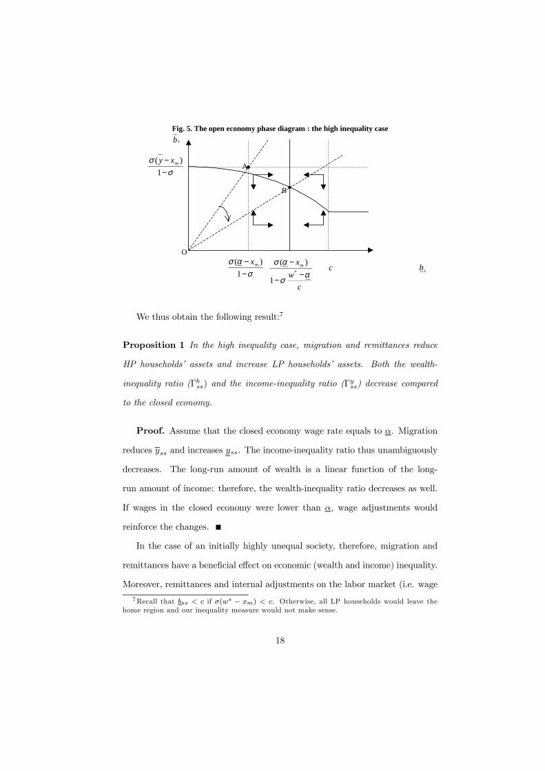
Fig. 5. The open economy phase diagram : the high inequality casetb

σσ

−−

1)( mxy

A

B

O

σ

ασ−−

1)( mx

cw

xm

ασ

ασ−

−

−*

1

)( c tb

We thus obtain the following result:7

Proposition 1 In the high inequality case, migration and remittances reduce

HP households’ assets and increase LP households’ assets. Both the wealth-

inequality ratio (¡bss) and the income-inequality ratio (¡yss) decrease compared

to the closed economy.

Proof. Assume that the closed economy wage rate equals to ®. Migration

reduces yss and increases yss. The income-inequality ratio thus unambiguously

decreases. The long-run amount of wealth is a linear function of the long-

run amount of income: therefore, the wealth-inequality ratio decreases as well.

If wages in the closed economy were lower than ®, wage adjustments would

reinforce the changes.

In the case of an initially highly unequal society, therefore, migration and

remittances have a bene…cial e¤ect on economic (wealth and income) inequality.

Moreover, remittances and internal adjustments on the labor market (i.e. wage

7Recall that bss < c if ¾(w¤ ¡ xm) < c. Otherwise, all LP households would leave thehome region and our inequality measure would not make sense.

18

responses) are both reducing inequality. This suggests that empirical models

based on Gini Index decomposition are likely to underestimate the impact of

migration on inequality by considering that the distribution of domestic earnings

is given.

4.2 The medium inequality case

The medium inequality case arises when ½(1 ¡ btc ) + w

¤ ¡ c < ® < 1 + ½(1 ¡btc ) +w

¤ ¡ c (i.e., on a limited range of values for ®). The equilibrium depends

on whether liquidity constraints are binding for HP households.

Non-biding liquidity constraints for HP households. If liquidity con-

straints are not binding, HP households select their optimal migration rate m¤

as given by equation (13). The demand for labor is the same as in the high

inequality case. In such a situation, HP households want to employ all LP

households’ members (ndt = 1) and this sets the wage rate at its maximal value

wt =®.

Given (6a)-(6b), the dynamics of wealth is characterized by the following

system:

bt+1 = ¾®(1¡ btc) + ¾(w¤ ¡ c)bt

c+ ¾bt ¡ ¾xm (16a)

bt+1 = ¾®(1 + ½¡ ½btc¡m¤)¡ ¾

2(1 + ½¡ ½bt

c¡m¤)2 (16b)

¡¾½®(1¡ btc) + ¾m¤(w¤ ¡ c) + ¾bt ¡ ¾xm

where m¤ = 1 + ½(1¡ btc ) +w

¤ ¡ c¡ ® 2 [0; 1] is the optimal migration rate ofHP households.

The corresponding phase diagram is represented on Figure 6. The closed

economy steady state equilibrium is at point A. The migration-and-remittances

process leads LP households to accumulate the same level of …nancial wealth as

19

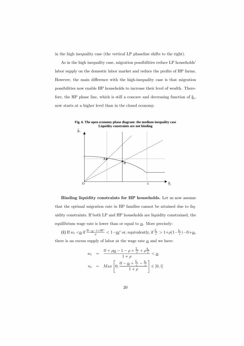
in the high inequality case (the vertical LP phaseline shifts to the right).

As in the high inequality case, migration possibilities reduce LP households’

labor supply on the domestic labor market and reduce the pro…ts of HP farms.

However, the main di¤erence with the high-inequality case is that migration

possibilities now enable HP households to increase their level of wealth. There-

fore, the HP phase line, which is still a concave and decreasing function of bt,

now starts at a higher level than in the closed economy.

Fig. 6. The open economy phase diagram: the medium inequality caseLiquidity constraints are not binding

tb

A B

O c tb

Binding liquidity constraints for HP households. Let us now assume

that the optimal migration rate in HP families cannot be attained due to liq-

uidity constraints. If both LP and HP households are liquidity constrained, the

equilibrium wage rate is lower than or equal to ®. More precisely:

(i) If wt <® if®¡®¡1+mc

½ < 1¡mc or, equivalently, if btc > 1+½(1¡ btc )¡®+®,

there is an excess supply of labor at the wage rate ® and we have:

wt =®+ ½®¡ 1¡ ½+ bt

c + ½btc

1 + ½< ®

nt = Max

"0;®¡ ®+ bt

c ¡btc

1 + ½

#2 [0; 1]

20

(ii) If wt =® if®¡®¡1+mc

½ > 1¡mc or, equivalently, if btc · 1+ ½(1¡ btc )¡

(® ¡ ®), there is an excess demand of labor at the wage rate ® and we havent = 1¡mc = 1¡ bt

c .

For illustrative purpose, let us focus on the second case with wt =®. Given

(6a)-(6b), the dynamics of wealth is characterized by the following system:

bt+1 = ¾®(1¡ nt ¡ btc)¡ ¾

2(1¡ nt ¡ bt

c)2 (17a)

+¾ntwt + ¾btc(w¤ ¡ c)bt

c+ ¾bt ¡ ¾xm

bt+1 = ¾®(1 + ½nt ¡ btc)¡ ¾

2(1 + ½nt ¡ bt

c)2 (17b)

¡¾½ntwt + ¾ btc(w¤ ¡ c) + ¾bt ¡ ¾xm

with wt and nt as de…ned above.

The dynamics is therefore non-linear. Both phase lines may be expressed

as the positive root of a second degree polynomial in bt. The same qualitative

results obtain when wt <®.

The typical representation is given in …gure 7. Point A represents the closed

economy equilibrium. Point B is the open economy equilibrium when liquidity

constraints are not binding for HP households (as depicted on …gure 6). When

liquidity constraints are binding, both phaselines are non linear and represented

by continuous curves. They only correspond to the unconstrained curves when

the assets of HP members exceed their ”optimal” migration costs, m¤c (i.e.,

above point X). Therefore, on …gure 7, liquidity constraints are only binding

below X.

The impact of liquidity constraints is to displace the HP phase line down-

wards. Then point B’ is the …nal steady state when liquidity constraints are

binding. The e¤ect of liquidity constraints on HP households, therefore, is to

21

further reduce the long-run level of assets of HP households and to increase the

level of assets within LP households. Hence, they reduce the wealth inequality

ratio: The slope of OB0 is lower than the slope of OB.

Fig. 7. The open economy phase diagram: the medium inequality caseLiquidity constraints are binding

tb

XA B

B’

O c tb

General result. Inequality is always decreased in the ”medium inequality

case” independently of whether liquidity constraints are binding for HP house-

holds:

Proposition 2 In the ”medium inequality case”, remittances and migration

reduce the level of assets of HP households and increase the level of assets of

LP households. Both the wealth-inequality ratio (¡bss) and the income-inequality

ratio (¡yss) are reduced once migration opportunities are introduced compared to

the closed economy.

Proof. Let us denote the long-run e¤ect of openness on HP households’

assets by ¢bss. Let us assume that: (i) liquidity constraints are not binding

(condition C1), and, (ii) both the pre- and post-migration local wages are given

by ® (condition C2). C2 requires that ½ < ®¡®-1. After some manipulations,one obtains ¢bss <

m2¡½2m2

2 . Using m = 1 + ½(1 ¡ bc ) + w

¤ ¡ c ¡ ® and

22

m = bc , it follows that ¢bss < 0 for ½(1¡ b

c )+w¤¡c < ®: the unconstrained HP

amount of assets decreases. If C1 does not hold (i.e., HP households are liquidity

constrained), the phase line shifts downwards and the e¤ect is even stronger.

If C2 does not hold (either the pre- or post-migration local wage is below ®),

a wage e¤ect reinforces the redistribution from HP to LP households. Finally,

since the long-run level of assets is a linear and increasing function of income,

migration reduces yss and increases yss: hence, ¡yss unambiguously decreases.

As in the high inequality case, openness to migration is not pareto-improving:

it improves the situation of LP households but reduces HP households’ income

and wealth.

4.3 The low inequality case

The ”low inequality case” holds for ® < ½(1¡ btc ) +w

¤ ¡ c (i.e., when the highincome class is not too di¤erent from the low income class). We assume that

the distribution of wealth is such that it cannot be that all HP members leave

the country (i.e., bt < c). Analytically, the low inequality case is equivalent to

the ”medium inequality case” when liquidity constraints are binding. However,

under the condition that ® < ½(1¡ btc ) + w

¤ ¡ c, the predictions on inequalitymay be di¤erent. More precisely:

Proposition 3 In the ”low inequality case”, remittances and migration in-

crease the amount of assets of LP households and have an ambiguous e¤ect

on the amount of assets of HP households. However, the wealth-inequality ratio

(¡bss) unambiguously decreases compared to the closed economy and the variation

in the income-inequality ratio (¡yss) may be either positive or negative.

23

Proof. Part 1. From Proposition 2, ½(1 ¡ bc ) + w

¤ ¡ c > ® implies that

¢bss S 0. Part 2. Let us assume that: (i) the post-migration amount of

HP assets equals to the migration cost (C1), and, (ii) both the pre- and post-

migration local wages are given by ® (C2). The property ¡bss < ¡b0 (where the

subscript 0 stands for the initial closed economy solution) may be rewritten as

c¡ ¾w¤ ¡ ¾® < ¾®(1 + ½)¡ ¾2 (1 + ½)

2 ¡ ¾®½¡ ¾xm. Using (17a) with bss = c(C1) and 1 + ½ < ®¡® (C2), this property becomes ¡½ bssc < 1, which always

holds. If either condition C1 or condition C2 do not hold, this reinforces the

result: liquidity constraints within HP households or an increase in the wage

rate both limit the rise in HP households’ assets and stimulate the rise in LP

households’ assets. Part 3. Using (8), the variation in the income ratio may be

expressed as:

¢¡y = ¡yss ¡ ¡y0 = (°ss ¡ °0) + (¡bss ¡ ¡b0) + (°0¡b0 ¡ °ss¡bss)

The …rst two terms are negative, meaning that the marginal propensity to save

among LP households increases and wealth inequality decreases (see part 2).

The third term is positive. The general e¤ect on income inequality is thus am-

biguous.

Fig. 7 also depicts the case of low initial inequality, except that the HP phase

line may shift above the closed economy phase line. Migration and remittances

can be pareto-improving compared to the closed economy solution. However,

the slope of OB’ is always lower than the slope of OA: wealth inequality is

always lower with migration. The major di¤erence with the medium inequality

case is that, as indicated in the proof of Proposition 3 above, income inequality

can be lower or greater than in the closed economy.

Numerical simulations illustrate these results. Consider the following pa-

rameters set: ® = 4:0, ®=1:25, ½ = 1:5, w¤ = 7:5, c = 2:0, ¾ = 0:15. Three

24

scenarios are distinguished: xm = 0:2 (scenario 1), xm = 0:4 (scenario 2) and

xm = 0:6 (scenario 3). The income inequality path (¡yt ) is represented on Fig.

8. In scenario 1, LP households’ marginal propensity to save is high; since mi-

gration and remittances give rise to an important wealth accumulation within

LP households, wealth and income inequality are reduced in the long-run. In

scenario 3, the opposite result emerges. In the intermediate scenario, the short-

run impact of remittances on inequality is negative while the long-run impact

is positive. This corresponds to the ”trickle-down” e¤ect suggested by Stark et

al. (1986 and 1988). Nevertheless, such a phenomenon is not due to the dynam-

ics of migration costs (which are kept constant in our simulations) but is fully

determined by the dynamics of wealth accumulation.

Fig. 8. Income inequality path

-15,0%

-10,0%

-5,0%

0,0%

5,0%

10,0%

0 1 2 3 4 5 6 7 8 9 10 11 12 13 14 15

Scenario 1 Scenario 2 Scenario 3

In the low inequality case, the inequality impact of remittances, on the one

hand, and of domestic wages, on the other hand, may be of opposite signs. While

wage responses always reduce the level of inequality (see …gure 4), remittances

can have a detrimental e¤ect on income dispersion. Most empirical models of

Gini index decomposition are only capturing the second e¤ect; however, evalu-

25

ating the global impact of migration on inequality requires endogenizing wage

dispersion as a function of migration ‡ows.

5 Conclusion

Our analysis sheds light on the short-run and long-run impact of migration and

remittances on economic inequality in the migrants’ communities of origin. This

impact largely depends on the initial distribution of wealth, which determines

migration incentives and opportunities.

A …rst result is that in the case of an initially highly unequal society, openess

to migration leads to a totally polarized economy with a class of poor salaried

workers and a class of rich landowners, and to a redistribution of wealth from

rich to poor households; since in our setting wealth and utility are identical

in the long-run, the induced changes are therefore not pareto-improving. In a

more homogenous society where rich households have an incentive to send some

members out, openness to migration may be pareto improving. In all cases,

however, migration and remittances bring about a decrease in wealth inequality

at origin.

A second result concerns income inequality. The relationship between in-

come and utility is linear but changes over time according to the evolution of

the propensity to save within poor households. Income- and wealth-inequality

responses to migration need not be identical in size and nature. In some realistic

cases, income inequality may be increased while wealth inequality decreases. In

addition, due to a combination of changes in people’s income and propensity

to save over time, income inequality may be characterized by a ”trickle-down”

transition path even if the dynamics of assets is basically monotonic. This could

be reinforced by the evolution of migration costs thanks to the role of migrants’

26

networks; however, migration network e¤ects are not a necessary condition for

observing such an inverse U-shaped inequality path.

A third result is that the inequality impacts of remittances, on the one hand,

and of local wages adjustments, on the other hand, tend to reinforce one another

when initial inequality is relatively high (high and medium inequality cases) but

may be of opposite signs in the low inequality case. This has strong implications

for empirical studies based on Gini Index decompositions with exogenous dis-

tributions of domestic incomes. Our framework suggests that such distributions

should be treated as endogenous, as advocated by Adams (1989), Taylor (1992)

or Braham and Boucher (1998). This also suggests that the lack of consensus

in the empirical literature on the inequality impact of migration may be partly

explained by the omission of labor market responses. Indeed, in a country such

as Mexico where inequality is high by international standards, this omission is

likely to lead to an underestimation of the inequality-reducing e¤ect of migra-

tion, but not to a reversal of the sign of the e¤ect. By contrast, in a country such

as Yugoslavia where inequality is much lower, taking labor market responses into

account could possibly reverse the …ndings of an inequality-enhancing e¤ect.

27

Finally, it holds true that the evolution of migration costs is crucial for

the determination of the long-run impact of migration and remittances. In all

cases, a drop in migration costs induces strong inequality-reducing e¤ects. The

short-run impact, however, is ambiguous. If rich and poor households are both

liquidity constrained, a drop in migration costs may well increase the inequality

ratio in the short-run since rich households derive more pro…ts from migration.8

Hence, a decrease in migration costs may generate higher inequality in the …rst

stages of the migration history. In the long-run, however, lower migration costs

are always bene…cial in terms of reduced economic inequality. These results are

consistent with the …ndings of the remittances-and-inequality empirical litera-

ture, but o¤er a di¤erent interpretation, with no need to endogenize migration

costs through network e¤ects.

6 References

Adams, R. (1989): Workers remittances and inequality in rural Egypt, Economic De-

velopment and Cultural Change, 38, 1: 45-71.

Adams, R. (1992): The impact of migration and remittances on inequality in rural

Pakistan, Pakistan Development Review, 31, 4: 1189-203.

Barham, B. and S. Boucher (1998): Migration, remittances and inequality: esti-

mating the net e¤ects of migration on income distribution, Journal of Development

Economics, 55: 307-31.

8To illustrate this result, consider the numerical example of scenario 2 and compare thedynamic paths with respectively c = 2:0 and c = 1:5. As depicted in Table 1, a drop inmigration costs raises the income ratio in period 1 and reduces the inequality rate thereafter,reinforcing the likelihood of observing a trickle down phenomenon.

Table 1: Policy analysis (e¤ect of openness on the income ratio in percent)Period 0 1 2 3 ssScen. 2 (c=2.0) 0.0% 2.9% 0.7% -1.4% -5.8%Scen. 2’ (c=1.5) 0.0% 3.4% -1.9% -12.9% -36.8%

28

Carrington, W.J., E. Detragiache and T. Vishwanath (1996): Migration with en-

dogenous moving costs, American Economic Review, 86 (4): 909-30.

Cox, D., Z. Eser and E. Jimenez (1998): Motives for private transfers over the

life cycle: An analytical framework and evidence for Peru, Journal of Development

Economics, 55: 57-80.

de la Briere, B., A. de Janvry, S. Lambert and E. Sadoulet (2002): The roles of

destination, gender, and household composition in explaining remittances: An analysis

for the Dominican Sierra, Journal of Development Economics, 68, 2: 309-28.

Djajic, S. (1986): International migration, remittances and welfare in a dependent

economy, Journal of Development Economics, 21: 229-34.

Dustmann, C. and O. Kirchkamp (2002): The optimal migration duration and

activity choice after remigration, Journal of Development Economics, 67, 2: 351-72.

Hoddinott, J. (1994): A model of migration and remittances applied to Western

Kenya, Oxford Economic Papers, 46(8): 459-76.

Ilahi, N. (1999): Return migration and occupational change, Review of Develop-

ment Economics, 3, 2: 170-86.

Ilahi, N. and S. Jafarey (1999): Guestworker migration, remittances and the ex-

tended family: evidence from Pakistan, Journal of Development Economics, 58: 485-

512.

Lucas, R.E.B. (1987): Emigration to South Africa’s mines, American Economic

Review, 77,3: 313-30.

Lucas, R.E.B. and O. Stark (1985): Motivations to remit: evidence from Botswana,

Journal of Political Economy, 93 (5): 901-18.

Massey, D.S, L. Goldring and J. Durand (1994): Continuities in Transnational

Migration: An Analysis of Nineteen Mexican Communities, American Journal of So-

ciology, 99, 6: 1492-1533.

29

McCormick, B. and J. Wahba (2000): Overseas unemployment and remittances to

a dual economy, Economic Journal, 110: 509-34.

McCormick, B. and J. Wahba (2001): Overseas experience, savings and entrepreneur-

ship amongst return migrants to LDCs, Scottish Journal of Political Economy, 48, 2:

164-78.

Mesnard, A. and M. Ravallion (2001): Wealth distribution and self-employment

in a developing economy, CEPR Discussion Paper No 3026.

Milanovic, B. (1987): Remittances and income distribution, Journal of Economic

Studies, 14(5): 24-37.

Munshi, K. (2003): Networks in the modern economy. Mexican migrants in the

US labor market, Quarterly Journal of Economics, 118, 2: 549-99..

Poirine, B. (1997): A theory of remittances as an implicit family loan arrangement,

World Development, 25(5): 589-611.

Rapoport, H. and F. Docquier (2003): The economics of migrants’ remittances; in

L.-A. Gerard-Varet, S.-C. Kolm and J. Mercier Ythier, eds.: Handbook of the Eco-

nomics of Reciprocity, Giving and Altruism, Amsterdam: North-Holland, forthcoming.

Rozelle, S., J.E. Taylor and A. deBrauw (1999): Migration, remittances and agri-

cultural productivity in China, American Economic Review, 78, 2: 245-50.

Stark, O., J.E. Taylor and S. Yitzhaki (1986): Remittances and inequality, Eco-

nomic Journal, 96(383): 722-40.

Stark, O., J.E. Taylor and S. Yitzhaki (1988): Migration, remittances and in-

equality: a sensitivity analysis using the extended Gini index, Journal of Development

Economics, 28: 309-22.

Taylor, J.E. (1992): Remittances and inequality reconsidered: direct, indirect and

intertemporal e¤ects, Journal of Policy Modeling, 14, 2: 187-208.

Taylor J.E. and T.J. Wyatt (1996), ”The Shadow Value of Migrant Remittances,

30

Income and Inequality in a Household-farm Economy”, Journal of Development Stud-

ies, 32, 6: 899-912.

Woodru¤, C. and R. Zenteno (2001): Remittances and micro-enterprises in Mexico,

Mimeo., University of California at San Diego.

31

IZA Discussion Papers No.

Author(s) Title

Area Date

794 P. Frijters M. A. Shields S. Wheatley Price

Investigating the Quitting Decision of Nurses: Panel Data Evidence from the British National Health Service

1 06/03

795 B. T. Hirsch Reconsidering Union Wage Effects: Surveying New Evidence on an Old Topic

3 06/03

796 P. Apps

Gender, Time Use and Models of the Household 5 06/03

797 E. Bratberg Ø. A. Nilsen K. Vaage

Assessing Changes in Intergenerational Earnings Mobility

2 06/03

798 J. J. Heckman J. A. Smith

The Determinants of Participation in a Social Program: Evidence from a Prototypical Job Training Program

6 06/03

799 R. A. Hart General Human Capital and Employment Adjustment in the Great Depression: Apprentices and Journeymen in UK Engineering

2 06/03

800 T. Beissinger C. Knoppik

Sind Nominallöhne starr? Neuere Evidenz und wirtschaftspolitische Implikationen

7 06/03

801 A. Launov A Study of the Austrian Labor Market Dynamics Using a Model of Search Equilibrium

2 06/03

802 H. Antecol P. Kuhn S. J. Trejo

Assimilation via Prices or Quantities? Labor Market Institutions and Immigrant Earnings Growth in Australia, Canada, and the United States

1 06/03

803 R. Lalive Social Interactions in Unemployment

3 06/03

804 J. H. Abbring Dynamic Econometric Program Evaluation

6 06/03

805 G. J. van den Berg A. van Vuuren

The Effect of Search Frictions on Wages 6 06/03

806 G. J. van den Berg Multiple Equilibria and Minimum Wages in Labor Markets with Informational Frictions and Heterogeneous Production Technologies

6 06/03

807 P. Frijters M. A. Shields N. Theodoropoulos S. Wheatley Price

Testing for Employee Discrimination Using Matched Employer-Employee Data: Theory and Evidence

5 06/03

808 F. Docquier H. Rapoport

Remittances and Inequality: A Dynamic Migration Model

1 06/03

An updated list of IZA Discussion Papers is available on the center‘s homepage www.iza.org.