Contents lists available at ScienceDirect

Remote Sensing of Environment

journal homepage: www.elsevier.com/locate/rse

Estimating surface soil moisture from SMAP observations using a NeuralNetwork technique

J. Kolassa*,a,b, R.H. Reichleb, Q. Liuc,b, S.H. Alemohammadd, P. Gentined, K. Aidae, J. Asanumae,S. Bircherl, T. Caldwellm, A. Collianderf, M. Coshg, C. Holifield Collinsn, T.J. Jacksong,J. Martínez-Fernándezh, H. McNairni, A. Pachecoi, M. Thibeaultj, J.P. Walkerk

a Universities Space Research Association/NPP, Columbia, MD, USAb Global Modelling and Assimilation Office, NASA Goddard Spaceflight Center, Greenbelt, MD, USAc Science Systems and Applications Inc., Lanham, MD, USAd Columbia University, New York, NY, USAe University of Tsukuba, Tsukuba, Japanf Jet Propulsion Laboratory, California Institute of Technology, Pasadena, CA, USAg USDA ARS Hydrology and Remote Sensing Laboratory, Beltsville, MD, USAh Instituto Hispano Luso de Investigaciones Agrarias (CIALE), Universidad de Salamanca, Salamanca, Spaini Agriculture and Agri-food Canada, Ottawa, Ontario, Canadaj Comisiòn Nacional de Actividades Espaciales (CONAE), Buenos Aires, Argentinak Department of Civil Engineering, Monash University, Clayton, Victoria, Australial Centre d’Etudes Spatiales de la BIOsphère, (CESBIO-CNES, CNRS, IRD, Université Toulouse III), Toulouse, Francem University of Texas at Austin, TX, USAn USDA ARS Southwest Watershed Research Center, Tucson, AZ, USA

A R T I C L E I N F O

Keywords:Soil moisture remote sensingSMAPData assimilationMicrowave radiometer

A B S T R A C T

A Neural Network (NN) algorithm was developed to estimate global surface soil moisture for April 2015 toMarch 2017 with a 2–3 day repeat frequency using passive microwave observations from the Soil MoistureActive Passive (SMAP) satellite, surface soil temperatures from the NASA Goddard Earth Observing SystemModel version 5 (GEOS-5) land modeling system, and Moderate Resolution Imaging Spectroradiometer-basedvegetation water content. The NN was trained on GEOS-5 soil moisture target data, making the NN estimatesconsistent with the GEOS-5 climatology, such that they may ultimately be assimilated into this model withoutfurther bias correction. Evaluated against in situ soil moisture measurements, the average unbiased root meansquare error (ubRMSE), correlation and anomaly correlation of the NN retrievals were 0.037 m3m−3, 0.70 and0.66, respectively, against SMAP core validation site measurements and 0.026 m3m−3, 0.58 and 0.48, respec-tively, against International Soil Moisture Network (ISMN) measurements. At the core validation sites, the NNretrievals have a significantly higher skill than the GEOS-5 model estimates and a slightly lower correlation skillthan the SMAP Level-2 Passive (L2P) product. The feasibility of the NN method was reflected by a lower ubRMSEcompared to the L2P retrievals as well as a higher skill when ancillary parameters in physically-based retrievalswere uncertain. Against ISMN measurements, the skill of the two retrieval products was more comparable. Atriple collocation analysis against Advanced Microwave Scanning Radiometer 2 (AMSR2) and AdvancedScatterometer (ASCAT) soil moisture retrievals showed that the NN and L2P retrieval errors have a similarspatial distribution, but the NN retrieval errors are generally lower in densely vegetated regions and transitionzones.

1. Introduction

Soil moisture is a key variable for many surface and boundary layerprocesses, such as the coupling of the water and energy cycles

(Seneviratne et al., 2006; Gentine et al., 2011; Bateni and Entekhabi,2012) or the partitioning of precipitation into runoff and infiltration(Philip, 1957, Corradini et al., 1998, Assouline, 2013). Soil moisture isalso a key determinant of the carbon cycle (McDowell, 2011; Sevanto

https://doi.org/10.1016/j.rse.2017.10.045Received 21 April 2017; Received in revised form 24 October 2017; Accepted 30 October 2017

* Corresponding author.E-mail address: jana.kolassa@nasa.gov (J. Kolassa).

Remote Sensing of Environment 204 (2018) 43–59

Available online 11 November 20170034-4257/ Published by Elsevier Inc.

T

et al., 2014; Jung et al., 2017). The importance of soil moisture hasbeen recognized by the World Meteorological Organization by namingit an Essential Climate Variable (GCOS, 2009) and thus encouragingefforts to obtain better soil moisture observations, which is challengingbecause of its high variability both in space and time.

One avenue to obtain observations of soil moisture is through sa-tellite instruments that provide global observations with a relativelyshort revisit period of 2–3 days. In particular, L-band (1.4 GHz) mi-crowave instruments exhibit a high sensitivity to soil moisture in thetop ∼5 cm of the soil in sparsely to moderately vegetated areas. Thishas led to the launch of two L-band satellite missions to observe soilmoisture, the European Soil Moisture and Ocean Salinity (SMOS) mis-sion in 2009 (Kerr et al., 2010) and the NASA Soil Moisture ActivePassive (SMAP) mission (Entekhabi et al., 2010) in 2015.

Traditionally, satellite soil moisture retrievals from L-band (andother) sensors are implemented through the inversion of RadiativeTransfer Models (RTMs) (e.g. Owe et al., 2001; Kerr et al., 2012; O’Neillet al., 2015), which explicitly formulate the physical relationshipslinking surface soil moisture to satellite brightness temperature ob-servations. The RTM inversion technique is used to produce the officialSMOS and SMAP retrieval products, and is able to provide high qualitysoil moisture estimates (Al Bitar et al., 2012; Chan et al., 2016b;Colliander et al., 2017) with a typical latency of 12 to 24 h. However,this approach requires accurate knowledge of the physical relationshipsbetween the surface state and the satellite observations as well as theirassociated parameters, which are often empirically estimated and thusuncertain. Moreover, RTM inversions also require explicit informationon other surface states, including surface soil temperature and vegeta-tion, and are thus typically ill-posed problems. Additionally, for timecritical applications, such as near real time flood prediction or soilmoisture assimilation into weather prediction models, retrieval pro-ducts with a shorter latency are required.

Data assimilation provides another option to generate improved soilmoisture estimates through the merging of satellite and model in-formation, and can yield soil moisture estimates that are of higherquality than estimates from satellite observations or models alone (e.g.Entekhabi et al., 1994; Walker and Houser, 2001; Liu et al., 2011; Lahozand De Lannoy, 2014). For soil moisture assimilation, the observationsand model estimates have to be unbiased with respect to each other,which is typically achieved by locally matching the mean and varia-bility of the satellite observations to those of the model (Reichle andKoster, 2004). While this satisfies the requirements of the assimilationsystem, it has the side effect of removing some independent informationin the satellite observations. Given the high quality of soil moistureobservations from SMOS and SMAP this is undesirable.

As an alternative to RTM inversions, statistical Neural Network(NN) retrieval algorithms have been successfully implemented for anumber of sensors in recent years (Aires et al., 2005; Chai et al., 2009;Kolassa et al., 2013, 2016; Rodríguez-Fernández et al., 2015; Santiet al., 2016). Instead of explicitly formulating physical relationships,NNs are calibrated on a sample of satellite observations and corre-sponding soil moisture estimates (the target data) to model the globalstatistical relationship between the satellite observations and surfacesoil moisture. As a result, NN retrievals can offer several general ad-vantages over traditional RTM inversions. First, they do not require anexplicit parameterization of physical relationships and are thus notaffected by errors in our knowledge of these relationships or theirparameters. Second, after a one-time calibration, NNs are computa-tionally extremely efficient and can provide soil moisture estimatesalmost immediately after arrival of the instrument data, therebyshortening the latency. Third, training a NN non-locally on target datafrom a model, yields NN retrievals that are globally unbiased with re-spect to the model, with spatial and temporal patterns that are drivenby the satellite observations (e.g. Alemohammad et al. (2017), Jimenezet al. (2013), Kolassa et al. (2016)). This may reduce the need for biascorrection prior to an assimilation and at the same time retain more of

the independent information contained in the spatial and temporalpatterns of the satellite observations.

In this study, we develop the first NN algorithm to retrieve globalsurface soil moisture from SMAP observations. The motivation for thiswork is twofold. First, we investigate statistical retrieval techniques as apossible alternative or supplement to the existing physically-basedSMAP retrieval algorithms. Since statistical techniques require lessancillary data and are subject to different algorithm-related errors thanphysically-based retrievals, NN retrievals may provide useful informa-tion where and when RTMs are known to be uncertain. For SMOS, theNN technique has been successfully implemented (Rodríguez-Fernández et al., 2015). However, it is not obvious that a NN for SMAPwill work equally well, given the differences between SMOS and SMAPin the observing geometry (multiple vs. single incidence angle) andinstrument error characteristics (De Lannoy et al., 2015). Second, weaim to investigate the potential of statistical techniques to generate asoil moisture product with characteristics beneficial to SMAP soilmoisture assimilation. The NN algorithm retrieves soil moisture in theclimatology of the target model and thus may reduce the need for biascorrection prior to data assimilation. In a follow-on study, we will in-vestigate whether this results in a more efficient use of SMAP ob-servations during data assimilation.

The NN retrieval algorithm is trained with SMAP brightness tem-peratures and two ancillary datasets as inputs, and with target datafrom the NASA Goddard Earth Observing System version 5 (GEOS-5)model (Section 2). Using the trained NN, we compute global estimatesof volumetric surface soil moisture for the period April 2015 to March2017 and evaluate them using a number of different metrics andtechniques (Section 3). We compare the SMAP NN soil moisture esti-mates to the target GEOS-5 model soil moisture to identify the in-dependent information provided by the SMAP observations that canpotentially inform the model during data assimilation (Section 4.1).Next, we assess the SMAP NN retrievals against independent in situmeasurements and compare their skill to that of the SMAP Level-2passive (L2P) retrieval product and the GEOS-5 model soil moisture(Section 4.2). Finally, we assess the global error distributions of theSMAP NN, GEOS-5 and SMAP L2P products using a triple collocation(TC) analysis in conjunction with soil moisture retrievals based onobservations from the Advanced Microwave Scanning Radiometer 2(AMSR2) and the Advanced Scatterometer (ASCAT), which have in-dependent errors with respect to the SMAP and GEOS-5 products(Section 4.3).

2. Datasets

2.1. Neural Network inputs and target datasets

2.1.1. SMAP observationsThe main input to the NN soil moisture retrieval algorithm are the

SMAP brightness temperatures. SMAP was launched in January 2015and is equipped with an L-band (1.4 GHz) radiometer observing on fourdifferent channels, horizontal and vertical polarization as well as the3rd and 4th Stokes' parameter. SMAP is in a sun-synchronous, near-circular orbit with equator crossings at 6 AM and 6 PM local time and arevisit time of 2–3 days (Entekhabi et al., 2010). Brightness tempera-ture data have been collected since 31 March 2015.

For our NN retrieval product we use SMAP Level-1C brightnesstemperatures (Chan et al., 2016) for the April 2015 to March 2017period. The data are provided on the 36-km resolution Equal-AreaScalable Earth version 2 (EASEv2) grid (Brodzik et al., 2012) as dailyhalf-orbit files. We only use observations from the 6 AM overpass, inorder to minimize observation errors due to Faraday rotation and thedifference between the soil and canopy temperatures (Entekhabi et al.,2010; O’Neill et al., 2015). A test of different input combinations in-dicated that using data from all four SMAP channels as inputs to theretrieval algorithm yielded the best NN retrieval performance (not

J. Kolassa et al. Remote Sensing of Environment 204 (2018) 43–59

44

shown). While the 3rd and 4th Stokes' parameters are not directlysensitive to soil moisture, including them as inputs helps the NN algo-rithm to distinguish between different observing conditions and thusdetermine the weight for a given brightness temperature observation.

2.1.2. GEOS-5 model surface soil moisture and temperatureThe model soil moisture estimates used here are generated using the

GEOS-5 Catchment land surface model (Koster et al., 2000; Ducharneet al., 2000). The Catchment model version used in this study is verysimilar to that of the SMAP Level-4 Soil Moisture (L4_SM) version 2system (Reichle et al., 2015, 2016, 2017b), but SMAP brightness tem-perature observations are not assimilated. The surface meteorologicalforcing data were provided at 0.25° resolution by the GEOS-5 ForwardProcessing atmospheric data assimilation system (Lucchesi, 2013). TheGEOS-5 precipitation forcing data were corrected using global, daily,0.5 ° resolution, gauge-based observations from the Climate PredictionCenter Unified (CPCU) product, which have been scaled to the GlobalPrecipitation Climatology Project (GPCP) v2.2 pentad precipitationproduct climatology (Reichle et al., 2017b; Reichle and Liu, 2014;Reichle et al., 2017a). The GEOS-5 background precipitation was alsoscaled to the GPCP v2.2 climatology. Output fields were produced as 3-hourly time averages and provided on the 9-km EASEv2 grid.

In this study, we use two model output fields: (1) the surface soilmoisture (0–5 cm soil layer) and (2) the surface soil temperature (0–10cm soil layer). The GEOS-5 soil moisture fields served as target data inthe NN training (Section 3.1) and were also used in the evaluationphase to assess the skill of the NN retrieval compared to that of thetarget model. The surface soil temperature data were used as an input tothe retrieval algorithm to account for the surface soil temperaturecontribution to the observed brightness temperatures (Section 3.1).Using surface soil temperature estimates from the target model poten-tially introduces some of the GEOS-5 spatial patterns into the NN es-timates and could lead to model dependency issues during a later as-similation of the NN estimates into the GEOS-5 model. The same wouldbe true, however, for the assimilation of the SMAP L2P product, whichalso uses GEOS-5 ancillary soil temperatures (Section 2.2.1). We assumehere that the canopy temperature and surface soil temperature are inequilibrium for the 6 AM (local time) SMAP observations used here, soonly a single temperature estimate is required. The surface soil tem-perature data were also used in the data quality control to identifyfrozen soil conditions (Section 2.3).

2.2. Validation datasets

2.2.1. SMAP Level-2 passive retrievalsThe SMAP L2P soil moisture retrieval product uses SMAP radio-

meter Level-1C brightness temperatures to provide soil moisture esti-mates on the 36-km EASEv2 grid as daily half-orbit files. The retrievalalgorithm is based on a physical tau-omega model (O’Neill et al., 2015;Wigneron et al., 1995) to isolate the soil emission from the total ob-served surface emission (soil and vegetation) and to subsequentlyconvert it into a soil moisture estimate through the use of soil emissionand mixing models. The surface soil temperature data required by thetau-omega model are provided by the quasi-operational GEOS-5 For-ward Processing system (Lucchesi, 2013) with a 0.25° resolution. Thetau-omega model also requires information on the vegetation watercontent (VWC), which is estimated from a climatology of the Normal-ized Difference Vegetation Index based on Moderate Resolution Ima-ging Spectroradiometer (MODIS) observations using an empirical re-lationship established from prior investigations. No retrieval isperformed for frozen soil conditions based on GEOS-5 surface soiltemperature. Soil moisture retrievals are flagged as ‘not recommended’when the VWC within the satellite footprint exceeds 5 kg m−2 (O’Neillet al., 2015).

In this study, we use version 4 of the L2P ‘baseline’ soil moistureestimates derived from the SMAP morning (6 AM) overpass vertical

polarization brightness temperatures (O’Neill et al., 2016). Only datapoints flagged as having the ‘recommended’ retrieval quality were used.

2.2.2. AMSR2 and ASCAT soil moisture retrievalsThe Advanced Multichannel Scanning Radiometer 2 (AMSR2) is a

multichannel passive microwave satellite instrument that has beencollecting data since July 2012. AMSR2 measures brightness tempera-tures at frequencies ranging from 6.9 GHz to 89 GHz with a revisit timeof approximately 2 days and equator crossings at 1.30 AM and 1.30 PMlocal time (Kasahara et al., 2012).

Here we use the Japan Aerospace Exploration Agency AMSR2 soilmoisture product computed from the 10.7 GHz and 36.5 GHz verticaland horizontal polarization brightness temperatures (Maeda andTaniguchi, 2013). The data are provided as daily estimates of volu-metric surface soil moisture on a grid with 0.1° × 0.1° resolutionspacing.

The Advanced Scatterometer (ASCAT) (Figa-Saldaña et al., 2002) isan active microwave satellite instrument aboard the MetOp satellites,which have been collecting data since 2006. ASCAT measures surfacebackscatter at C-band (5.3 GHz) with a revisit time of 1–2 days andequator crossings at 9.30 AM and 9.30 PM.

Here we use the ASCAT surface soil moisture product developed byWagner et al. (2013). The data are provided in units of surface degree ofsaturation with a sampling distance of 12.5×12.5 km and were con-verted into estimates of volumetric surface soil moisture using the soilporosity data of Reynolds et al. (2000).

Despite being posted on finer resolution grids, the spatial resolutionof the AMSR2 and ASCAT observations is very similar to the SMAP 36-km resolution.

2.2.3. In situ measurements2.2.3.1. SMAP core validation sites. The SMAP core validation sites(referred to here as ‘core sites') represent locally dense networks of insitu soil moisture measurements that are specifically designed for thecalibration and validation of SMAP soil moisture products (Collianderet al., 2017). Each site features an array of soil moisture sensors torepresent the different spatial scales of the SMAP products (3 km, 9 kmand 36 km). The measurements from each site's sensors are combinedinto and area-weighted average to yield one soil moisture time seriesper site that is representative of a 36-km satellite grid cell.

Table 1 summarizes the main characteristics of the 36-km core sitesused here. Out of the 14 locations, nine are in North America, two inEurope, and one each in Asia, Australia and South America. The sitesrepresent a range of different climatic conditions and land cover types,and the average number of sensors that contribute to the 36-km re-ference pixel data ranges between 5 and 32. Fig. 1 shows the dis-tribution of the SMAP core sites and their corresponding dominant landcover.

2.2.3.2. International Soil Moisture Network (ISMN). We furtherevaluate the NN retrieval product against independent in situ soilmoisture measurements from the International Soil Moisture Network(ISMN), a database of soil moisture networks hosted at the TechnicalUniversity (TU) of Vienna (Dorigo et al., 2011) and referred to here asthe ‘sparse networks'. We used only ISMN networks that are not part ofthe SMAP core sites (Table 2). The REMEDHUS network comprises adifferent set of sensors for the core site and as a sparse network and thusappears for both in situ data types. The measurement depth, repeatfrequency, coverage, station density and measurement method dependon the contributing network. The number of stations in each networkranges between 1 and 441 (Table 2), but - unlike for the core sites -there is typically only one sensor per 36-km grid cell. That is, the ISMNmeasurements are not necessarily representative of the spatial scale ofthe satellite observations. Fig. 1 shows the spatial distribution of theISMN stations and the dominant land cover at each location.

For two of the ISMN networks, SCAN (Schaefer et al., 2007) and

J. Kolassa et al. Remote Sensing of Environment 204 (2018) 43–59

45

USCRN (Diamond et al., 2013), the data were already available in-house and had been subjected to additional quality control as describedin De Lannoy et al. (2014) and (Reichle et al., 2015b) (their AppendixC). Hence, the in-house data were used for SCAN and USCRN instead ofthe data provided through the ISMN. As a result, more reliable metricscould be estimated for these two sparse networks.

2.3. Data preprocessing

2.3.1. Satellite observations and modelWe co-located all datasets spatially and temporally, using the 36-km

EASEv2 grid and the SMAP morning (6 AM) overpass times as a re-ference. The GEOS-5, AMSR2 and ASCAT data were aggregated fromtheir higher-resolution native grids to the 36-km EASEv2 grid usingsimple averaging. The temporal co-location was implemented by usingthe GEOS-5 3-hourly average that includes the SMAP morning overpassfor a given location and day. For the AMSR2 and ASCAT retrievalproducts, only data from their night-time/morning overpasses for thesame day - at 1.30 AM and 9.30 AM, respectively - were used sincethese are closest in time to the SMAP overpass at 6 AM. Likewise, forthe L2P retrievals we used only the morning overpass estimates, and noregridding was required because the SMAP-based NN and L2P productsare provided on the same 36-km EASEv2 grid.

We additionally applied several quality control steps to the satellite

and model data sets to identify and exclude conditions in which a soilmoisture retrieval was not feasible. Using the GEOS-5 surface soiltemperature, we excluded times and locations with a surface soil tem-perature below 1°C. The MODIS-based VWC estimates provided withthe L2P data were used to exclude times and locations with a VWChigher than 5 kg m−2, where the SMAP radiometer is not expected toprovide reliable retrievals. Finally, we excluded all pixels within 72 kmof a water body - defined as a grid cell with a water fraction in excess of

Table 1Overview of the SMAP Cal/Val core sites. Shown are (from left to right) the site name, reference pixel ID (RPID), location, climate, land cover and the average number of sensors thatcontribute to the reference pixel average. Soil moisture is measured at 5 cm depth or over the top 5 cm. (Colliander et al., 2017).

Site (abbreviation) RPID Location Climate Land cover Number of sensors

REMEDHUS (RM) 03013602 Spain Temperate Croplands 14Reynolds Creek (RC) 04013601 USA (Idaho) Arid Grasslands 5Yanco (YC) 07013601 Australia Arid Croplands 26Carman (CM) 09013601 Canada Cold Croplands 19Twente (TW) 12043602 Holland Temperate Croplands/natural mosaic 9Walnut Gulch (WG) 16013603 USA (Arizona) Arid Shrub open 20Little Washita (LW) 16023602 USA (Oklahoma) Temperate Grasslands 16Fort Cobb (FC) 16033602 USA (Oklahoma) Temperate Grasslands 12Little River (LR) 16043602 USA (Georgia) Temperate Croplands/natural mosaic 19South Fork (SF) 16073602 USA (Iowa) Cold Croplands 18Monte Buey (MB) 19023601 Argentina Temperate Croplands 10Kenaston (KN) 27013601 Canada Cold Croplands 26TxSON (TX) 48013601 USA (Texas) Temperate Grasslands 32Mahasri (MH) 53013601 Mongolia Cold Grasslands 5

YC

MHTWRMLRSFCMKN

RC

FC

LW

WG

TX

MB

Fig. 1. Location of the SMAP core validation sites (blue circles) and ISMN stations (red crosses). The background shows the dominant International Geosphere-Biosphere Program (IGBP,(Belward et al., 1999)) land cover class for each location.

Table 2Overview of the ISMN (Dorigo et al., 2011). Shown are the location, number of stationsper network and the network-specific reference.

Network Location # Stations Reference

Dahra Senegal 1 Tagesson et al. (2015)FMI Finland 27 Dorigo et al. (2011)iRON USA 6 Taylor et al. (2015)PBO H2O USA 161 Larson et al. (2008)REMEDHUS Spain 24 Sanchez et al. (2012)RSMN Romania 20 Dorigo et al. (2011)SCAN USA 181 Schaefer et al. (2007)SMOSMANIA France 21 Calvet et al. (2007)SNOTEL USA 441 Leavesley et al. (2008)SOILSCAPE USA 171 Moghaddam et al. (2016)USCRN USA 115 Diamond et al. (2013)

J. Kolassa et al. Remote Sensing of Environment 204 (2018) 43–59

46

5% according to the GEOS-5 land mask - to mitigate the impact of waterbodies, as their low brightness temperatures cause erroneously high soilmoisture retrievals (O’Neill et al., 2015).

2.3.2. In situ dataThe core site measurements are representative of the 36-km spatial

resolution of the retrievals and the aggregated model, however, thegeographical center of the in situ sensors for a given reference pixeldoes not generally coincide with the EASEv2 grid cell center of thesatellite and model products. Similarly, the location of a (single point)ISMN measurement is typically offset from the center of a EASEv2 gridcell. To account for this, the retrieval and (aggregated) model soilmoisture were linearly interpolated to the in situ location using datafrom the nearest EASEv2 grid cell and its 8 surrounding neighbors,requiring a minimum of 4 data points. Where applicable, ISMN mea-surements located in the same EASEv2 grid cell were averaged and theiraverage location was used for the interpolation. For each day, the insitu measurement closest in time and within a 3 h window of the SMAPoverpass was used.

Using the GEOS-5 surface temperature for the ISMN measurementsand the in situ surface soil temperature observations for the core sitemeasurements, the in situ data were screened for (nearly) frozen soilconditions by applying the same 1°C threshold that was used for thesatellite and model data.

3. Methodology

3.1. Neural Network retrieval algorithm

In this study we use a NN approach to retrieve global surface soilmoisture with a 2–3 day repeat using SMAP brightness temperatures,GEOS-5 soil temperatures and the MODIS-based VWC climatology thatis used in the generation of the SMAP L2P product. The NN retrievalalgorithm is first calibrated (trained) using a subset of the availableSMAP and model data to determine the statistical relationship betweenthe satellite observations and surface soil moisture. Once calibrated, thetrained NN is used to retrieve surface soil moisture from the entire set ofsatellite observations.

3.1.1. Neural Network architectureA neural network is a group of computational nodes arranged in a

layered and inter-connected architecture. Fig. 2 shows a schematic of abasic NN for soil moisture retrievals. The NN used here consists of 3layers: (1) an input layer that receives the satellite observations andancillary inputs, (2) one hidden layer, and (3) an output layer thatproduces the soil moisture estimates. This architecture is sufficient toapproximate any continuous function (Cybenko, 1989). The inputs forthe SMAP NN retrieval algorithm are the observations from the fourSMAP channels, the GEOS-5 surface soil temperature and the MODIS-based VWC estimates. The output from the NN algorithm is an estimateof the volumetric surface soil moisture.

While the number of neurons in the input and output layers is de-termined by the number of input and output variables (here, 6 for theinput layer and 1 for the output layer), the optimal number of neuronsin the hidden layer depends on the problem complexity. We found thatfor this study 15 hidden layer neurons constituted the lowest number ofneurons that was able to converge to a solution during the NN training.We use a fully connected feed-forward network, in which all neuronsfrom one layer are connected to all neurons in the next layer. Theseconnections are assigned weights - the synaptic weights - used by eachneuron to compute a weighted sum of all its input plus a bias beforeapplying a transfer function. Neurons in the input and output layers usea linear transfer function, while hidden layer neurons use the typicaltangent-sigmoid transfer function.

3.1.2. Neural Network trainingIn order to determine the statistical function that relates the NN

input data, including the satellite brightness temperature observations,to surface soil moisture, the NN is calibrated on a sample set of NNinputs and coincident soil moisture estimates (the target data), togetherreferred to as the training data. This process is referred to as the NNtraining and is schematically illustrated in Fig. 3 (a). To generate atraining dataset representative of all expected conditions, we used thefirst year (April 2015–March 2016) of our study period for NN training.The second year (April 2016–March 2017) of the study period was usedfor the evaluation presented in Sections 4.1 and 4.2. Model soilmoisture estimates from GEOS-5 are used as the target data, because (1)the model estimates have a similar resolution as the satellite observa-tions while providing complete spatio-temporal coverage and (2)training on a model yields NN estimates in the global model clima-tology, which could be beneficial for a later assimilation of the retrievedsoil moisture.

The total training dataset is split into three subsets - the calibration,validation and test data - by sampling the total dataset. The calibrationdata constitute 60% of the total training data and are used to optimizethe NN synaptic weights (Note: In the literature these data are oftenreferred to as ‘training data’. In order to avoid confusion with the totaltraining dataset, we have decided to use the term ‘calibration data’instead). The validation data constitute 20% of the total training dataand are used to detect over-fitting of the NN weights (see below). Theseare part of the training data and should not be confused with the in-dependent evaluation data used in Sections 4.1 and 4.2 to assess theSMAP NN retrieval quality. The test data constitute the remaining 20%of the training data and are used to assess the NN fit.

The NN training is non-localized, meaning that one NN is fitted to aglobal training dataset that contains data from the entire trainingperiod (April 2015–March 2016). Furthermore, no information re-garding the location and acquisition time of the training points isprovided to the NN. The NN training thus essentially involves an as-sociation of the same sets of input values (that is, the same brightnesstemperatures, Stokes' parameters, and ancillary data) with the meanvalue of the corresponding target soil moisture data. If, for example, thetarget data in a specific region overestimate the soil moisture, they willappear as outliers in the NN training, and the NN will thus not inheritsuch regional errors (e.g., (Jimenez et al., 2013)). As a result, the spatialand temporal patterns of the NN estimates are mostly driven by theinput satellite observations. Moreover, the NN estimates match theglobal (single-value) mean and variability of the target data, but meandifferences in the spatial patterns between the satellite observations andthe model estimates are retained. These remaining local biases couldrepresent an issue during an assimilation of the NN product. Furtherinvestigation will be needed to determine whether the disadvantage oflocal biases in the assimilation is outweighed by the benefit of retainingmore of the independent information in the assimilated SMAP ob-servations.

The training itself consists of an iterative optimization of the NNsynaptic weights to minimize the error between the NN output and thetarget data (Fig. 3 (a)). Three different scenarios cause the NN trainingto stop. First, the training is stopped when the mean squared errorbetween the NN outputs and the target data is less than 0.001 m3m−3

and the training goal is met. Second, the training is stopped when theNN training does not converge to a solution after a maximum number ofiterations - set here at 1000. Third, training is stopped when over-fittingof the NN weights to the calibration data is detected. For this, the errorbetween NN estimates computed from the validation input data and thevalidation model soil moistures is estimated upon each iteration. Adivergence of the validation estimates from the corresponding valida-tion model soil moisture indicates an over-fitting of the NN weights tothe calibration data and a loss of the NN's generalization ability. Whensuch a divergence is detected for six subsequent iterations, the trainingis stopped and the weights from the last iteration before the occurrence

J. Kolassa et al. Remote Sensing of Environment 204 (2018) 43–59

47

Fig. 2. Schematic of a Neural Network with close-up of asingle neuron (adapted from Kolassa (2013)).

Fig. 3. The two phases of the NN soil moisture retrieval approach. (a) NN training and (b) soil moisture estimation using the trained network. NN inputs include the SMAP brightnesstemperatures at vertical and horizontal polarization (Tbv and Tbh), the 3rd and 4th Stokes' parameters (Tb3 and Tb4), the GEOS-5 surface soil temperature (Ts), and the MODIS-basedvegetation water content (V WC).

J. Kolassa et al. Remote Sensing of Environment 204 (2018) 43–59

48

of the divergence are used as the final solution.Here we use a Levenberg-Marquardt training algorithm (Levenberg,

1944; Marquardt, 1963) and apply an error back-propagation approach(Rumelhart and Chauvin, 1995) to update the weights. The Levenberg-Marquardt algorithm stops when a local minimum is found and thusdoes not permit a full exploration of the error surface. To account forthis, the NN training is repeated four times, using a different randominitialization for the NN weights (and thus a different starting point onthe error surface) each time. This corresponds to four repetitions of thetraining process illustrated in Fig. 3 (a). After the training is stopped,we compute the root mean square error (RMSE) between the NN esti-mates computed from the test data and the corresponding test modelsoil moistures to assess the NN fit. The NN with the lowest RMSE errorout of the four repetitions is then retained as the optimal NN and usedto generate the soil moisture retrieval product.

The trained NN is used to compute global estimates of volumetricsoil moisture from the complete set of satellite observations and an-cillary data (Fig. 3 (b)). The soil moisture estimates are computed forthe period April 2015 to March 2017 and include both the training data(first year) and the evaluation data (second year) that were not used inthe training phase.

3.2. Evaluation metrics

As part of the NN retrieval development, we evaluate our retrievalproduct against in situ soil moisture measurements and assess its fitwith respect to the target model. To quantify different aspects of theretrieval product and model skill, we use the correlation R, anomalycorrelation Ranom and unbiased root mean square error ubRMSE. Thesemetrics have been chosen, because they evaluate different aspects of theretrieval products and provide complementary information on theproduct skill. Additionally, they are well-established for the evaluationof soil moisture retrievals (Al Bitar et al., 2012; Albergel et al., 2013;Chan et al., 2016b; Colliander et al., 2017). The evaluation metrics arecomputed with respect to the model soil moisture estimates(Section 4.1) and in situ measurements (Section 4.2).

The correlation (R) estimates the ability to capture soil moisturevariations at all time scales and is computed as the Pearson correlationcoefficient between the raw soil moisture and reference data time seriesin each location. The anomaly correlation (Ranom) estimates the abilityto capture individual drying and wetting events and is computed si-milarly to the correlation, but using the anomaly time series, with theanomalies defined with respect to the 30-day moving average centeredon the current day. The ubRMSE measures the RMSE excluding the biasand is computed after removing the long-term mean from the soilmoisture and reference data time series in each location. When asses-sing the fit between the NN retrieval product and its target model(Section 4.1), we use the term unbiased root mean square difference(ubRMSD) to indicate that the target model is not considered the truthin this case. Rather, the ubRMSD simply aims to identify differencesbetween the observed and modeled soil moistures.

When evaluating the skill of the retrieval and model productsagainst in situ measurements, only data points common to all fourdatasets (i.e., the NN and L2P retrievals, GEOS-5 model estimates, andin situ measurements) contributed to the metric calculations, with aminimum of 30 data points required. For the evaluation against ISMNdata, we report the average metrics across all stations in a network.Following the approach used by De Lannoy and Reichle (2016), weemploy a k-means clustering to avoid a dominance of areas with a highstation density and to obtain realistic confidence intervals. The spatialextent of each cluster is limited to 1° around its center. Additionally, wereport average metrics computed across all sites for the evaluationagainst core site data and across all networks for the evaluation againstthe ISMN data, applying the same clustering approach.

3.3. Triple collocation analysis

The evaluation of the NN retrieval product against in situ observa-tions is limited by the availability of the in situ measurements and thusonly covers a limited range of climate regions and land cover types.However, for most applications, and in particular for data assimilation,retrieval error estimates are required for every location. Here, we im-plement a triple collocation (TC) analysis (Stoffelen, 1998; McCollet al., 2014) in order to compute a global map of error estimates for theNN soil moisture product.

Triple collocation resolves the linear relationships between threeindependent datasets of the same variable (here, soil moisture) in orderto estimate the errors in each dataset independent of a reference. It is alocalized technique that estimates the errors for all three datasets ineach location independently, yielding a map of error estimates. Severalstudies have successfully applied TC to estimate soil moisture retrievalerrors (e.g., Scipal et al., 2008; Draper et al., 2013; Su et al., 2014; Chenet al., 2017). Here, we use TC to estimate the NN retrieval producterrors and, for comparison, the errors of the GEOS-5 model and L2P soilmoisture. However, one of the main assumptions of the TC analysis isan independence of the errors in the three datasets that constitute thetriplet. In the case of the NN, GEOS-5 and L2P products this assumptioncannot be made, since the NN uses information from the GEOS-5 modelwhile the NN and L2P retrievals rely on the same satellite input data.We therefore use the independent soil moisture retrieval products fromAMSR2 and ASCAT (Section 2.2.2) to create three suitable triplets:[SMAP NN, AMSR2, ASCAT], [GEOS-5, AMSR2, ASCAT] and [SMAPL2P, AMSR2, ASCAT]. This allows us to derive error estimates for SMAPNN, GEOS-5 and SMAP L2P.

Following McColl et al. (2014) and Draper et al. (2013), we applythe extended TC to the anomaly soil moisture time series (Section 3.2)and compute an error estimate in each location with at least 10common data points in the three contributing datasets. A bootstrappingapproach with 100 samples is applied to ensure a robust error estima-tion. To mitigate the error dependence on the (product- and location-specific) soil moisture variability, we estimate the fractional errorstandard deviation (Draper et al., 2013; Gruber et al., 2016), definedhere as the error standard deviation divided by the soil moisture stan-dard deviation of the corresponding product in each location. Thefractional error standard deviation is an approximation of the noise-to-signal ratio, with values below 1 indicating that the noise is smallerthan the signal and values greater than 1 indicating that the noise ex-ceeds the signal.

4. Results and discussion

4.1. Neural Network fit

As a first assessment, we compare the NN soil moisture estimates tothe GEOS-5 modeled soil moisture used as the target data. The purposeof this is to (1) assess the NN fit with respect to the target data over thetraining period, (2) evaluate the NN's ability to generalize beyond thetraining data and (3) identify areas of disagreement between the SMAPdriven NN estimates and the model soil moisture. In such areas, anassimilation of the NN retrievals should result in the largest changes tothe model.

Over the training period, the domain average ubRMSD, correlationand anomaly correlation between the NN and GEOS-5 soil moistures are0.037 m3m−3, 0.60 and 0.53, respectively. These fit values are typicalfor daily NN soil moisture retrievals (for example (Kolassa et al.,2016)). For the NN training it is not desirable to obtain a perfect fit withrespect to the target data, since the non-localized calibration results inspatial and temporal patterns that are driven by the satellite inputobservations and are thus expected to differ from patterns in the targetdata (Jimenez et al., 2013). Nevertheless, the fairly high correlation andlow ubRMSD values indicate that the SMAP based NN soil moisture

J. Kolassa et al. Remote Sensing of Environment 204 (2018) 43–59

49

-150 -100 -50 0 50 100 150

Longitude [deg]

-40

-20

0

20

40

60

80

Latit

ude

[deg

]

0

0.1

0.2

0.3

0.4

0.5

0.6

0.7

0.8

0.9

1

correlation [-]

-150 -100 -50 0 50 100 150

Longitude [deg]

-40

-20

0

20

40

60

80

Latit

ude

[deg

]

0

0.1

0.2

0.3

0.4

0.5

0.6

0.7

0.8

0.9

1

anomaly correlation [-]

-150 -100 -50 0 50 100 150

Longitude [deg]

-40

-20

0

20

40

60

80

Latit

ude

[deg

]

0

1

2

3

4

5

6

7

8

ubRM

SD

[m3 m

-3]

× 10 -3

(a) (b)

(c)-150 -100 -50 0 50 100 150

Longitude [deg]

-40

-20

0

20

40

60

80

Latit

ude

[deg

]

-0.02

-0.015

-0.01

-0.005

0

0.005

0.01

0.015

0.02

bias [m3 m

-3]

(d)

Fig. 4. (a) Correlation, (b) anomaly correlation, (c) ubRMSD and (d) bias between the SMAP NN soil moisture retrievals and the GEOS-5 model soil moisture for data points from theevaluation period (April 2016–March 2017). White spaces indicate areas with less than 30 data points, for which no robust metric could be computed.

0

20

40

60

80

100

prec

ipita

tion

[mm

]

-0.15

-0.1

-0.05

0

0.05

0.1

0.15

-0.15

-0.1

-0.05

0

0.05

0.1

0.15

-0.15

-0.1

-0.05

0

0.05

0.1

0.15

anom

aly

soil

moi

stur

e [m

3 m

-3]

anom

aly

soil

moi

stur

e [m

3 m

-3]

SMAP NN GEOS-5 SMAP L2P in situ precip

0

20

40

60

80

100

prec

ipita

tion

[mm

]

6102-016102-706102-405102-015102-705102-40

0

20

40

60

80

100

prec

ipita

tion

[mm

]

6102-016102-706102-405102-015102-705102-40

6102-016102-706102-405102-015102-705102-40

time [dd-mm-yyyy]

anom

aly

soil

moi

stur

e [m

3 m

-3]

(b) Walnut Gulch

(c) Carman

(a) TxSON

Fig. 5. Soil moisture anomalies with respect to a 30-day moving average at the (a) TxSON, (b) Walnut Gulch and (c) Carman core sites for April–September of 2015 and 2016. Shown arethe SMAP NN retrievals (red squares), the GEOS-5 model soil moisture (blue diamonds), the SMAP L2P retrievals (green circles) and the core site in situ soil moisture measurements(magenta triangles). Gray bars indicate the corrected GEOS-5 precipitation (Section 2.1.2) interpolated to the ground station site. The gray background shading indicates data belongingto the training period.

J. Kolassa et al. Remote Sensing of Environment 204 (2018) 43–59

50

corresponds with the estimates generated by the model in most regions.To assess the NN's ability to generalize beyond the training dataset

and to investigate the spatial distribution of the differences between theNN estimates and the GEOS-5 soil moisture, we also compared bothdatasets over the evaluation period, i.e., using only data points thatwere not part of the training dataset. Fig. 4 shows maps of the ubRMSD,correlation, anomaly correlation and bias between the NN estimatesand the model soil moisture. Averaging across these maps yields aubRMSD, correlation and anomaly correlation of 0.037 m3m−3, 0.61and 0.55, respectively, which are similar to the average metrics ob-tained for the training period and indicate that the NN is able to gen-eralize beyond the training dataset.

The correlations (Fig. 4 (a)) and anomaly correlations (Fig. 4 (b))exhibit similar spatial patterns, with high values in the transition zonesbetween wet and dry climates and in regions with strong soil moisturevariability, such as the Sahel, Eastern Brazil and India. However, strongcorrelations and anomaly correlations are also observed in semi-arid,sparsely to moderately vegetated regions, such as the Western US, theArabian Peninsula and large parts of Australia. The (anomaly) corre-lations are lowest in arid regions (e.g., the Sahara and Central Aus-tralia), where the soil moisture signal tends to be small and noisy, aswell as in extensive cropland regions (e.g., the US corn belt or thecroplands of Argentina, Uruguay and Paraguay), where irrigation and

other agricultural practices are likely to cause differences between thesatellite retrieval product and the model.

The spatial patterns of the ubRMSD between the SMAP NN esti-mates and the GEOS-5 soil moisture (Fig. 4 (c)) are different from thoseobserved for the (anomaly) correlations, with large portions of theglobe showing a ubRMSD of less than 0.001 m3m−3, including Africa,Australia and large parts of South America (excluding the Andes).Larger differences occur near mountainous regions, such as the RockyMountains or the Southern Andes, likely caused by higher uncertaintyin the SMAP retrieval product. High-latitude boreal regions, where thedata availability is low and the model precipitation forcing is less re-liable (Reichle and Liu, 2014), also exhibit larger differences betweenthe NN retrieval product and the model. Finally, the ubRMSD betweenthe NN retrievals and the model estimates is large in the croplands ofthe US as well as Southern Russia and Kazakhstan, which is possibly aresult of the missing representation of irrigation and other agriculturalpractices in the model that is being corrected by the NN.

The bias between the NN estimates and the GEOS-5 model over thetraining period (Fig. 4 (d)) ranges between −0.02 m3 m−3 and 0.02 m3

m−3 and, by design, has a global average close to zero. In arid regionssuch as the Arabian Peninsula, Central Australia or the Kalahari, the NNretrievals tend to indicate wetter conditions than the GEOS-5 model. Anexception is the Western Sahara, where the NN retrievals show a dry

SMAP NN GEOS-5 SMAP L2P

0

0.02

0.04

0.06

0.08

ubR

MS

E [m

3 m

-3]

0

0.2

0.4

0.6

0.8

1

corr

elat

ion

[-]

0

0.2

0.4

0.6

0.8

1

anom

aly

corr

elat

ion

[-]

RM

RC YC

CM

TW

WG

LW

FC LR

SF

MB

KN TX

MH

All

(a)

(b)

(c)

Fig. 6. (a) Correlation, (b) anomaly correlation and (c) ubRMSE between the core site in situ measurements and the SMAP NN retrievals (red squares), the SMAP L2P retrievals (greencircles) and the GEOS-5 model soil moisture (blue diamonds). Shown are the metrics for each site as well as the average across all sites. The error bars represent the 95% confidenceinterval.

J. Kolassa et al. Remote Sensing of Environment 204 (2018) 43–59

51

bias with respect to the GEOS-5 estimates, which might be an artifact ofincreased surface roughness in this region that lowers the observed soilemissivity.

In order to illustrate the behavior of the NN retrievals relative to theGEOS-5 model soil moisture in the training and evaluation periods,Fig. 5 shows the anomaly time series with respect to a 30-day movingaverage of the NN soil moisture estimates (red squares) and the GEOS-5model soil moisture (blue diamonds) for three SMAP core site stations -TxSON, Walnut Gulch and Carman. (The figure also shows the in situand L2P data, which will be discussed in Section 4.2.1.) For betterreadability and to reduce the effect of seasonal differences, we only plotthe months April–September for 2015 and 2016 to represent thetraining and evaluation periods, respectively, with the former indicatedthrough gray background shading. There is no obvious difference be-tween the behavior of the NN retrieval product in both periods, un-derlining once more the ability of the trained NN to generalize beyondthe training dataset. For the TxSON (Fig. 5 (a)) and Walnut Gulch(Fig. 5 (b)) sites, the time series average and dynamic range of the NNretrieval product and the GEOS-5 soil moisture are comparable, butthere are differences in the response to individual events, illustrated forinstance during the stronger drying in the NN soil moisture at theTxSON station in June 2015. At the Carman site (Fig. 5 (c)), the NN soilmoisture has a stronger variability compared to the model. This illus-trates that while the NN estimates globally match the bias and varia-bility of the target data, local biases and differences in variability be-tween the NN estimates and the target data occur.

4.2. Evaluation against in situ observations

In this section, we evaluate the skill of the NN retrieval productagainst independent in situ soil moisture measurements from the SMAPcore sites and the ISMN (Section 2.2.3). The skill of the NN retrievals iscompared against that of the GEOS-5 model soil moisture and the L2Pretrievals. Only data from the period April 2016–March 2017 are usedin the evaluation, since these data did not contribute to the NN training.

4.2.1. Core site dataFirst, we assess the skill of the soil moisture products against core

site in situ measurements. The NN retrieval product has a higher cor-relation than the GEOS-5 soil moisture for most core sites (Fig. 6 (a)),which is reflected in the higher average correlation of 0.70 for the NNretrievals compared to 0.64 for the model. The model has higher cor-relations than both retrieval products at Reynolds Creek and a highercorrelation than the NN retrievals at Carman and Kenaston. TheCarman and Kenaston watersheds are both located at high latitudeswhere an incomplete seasonal cycle due to frozen soil filtering couldprevent the NN from accurately learning the SM-Tb relationship forsuch conditions in the training phase. The NN retrievals tend to have anotably higher skill than the model in moderately vegetated regions,such as the shrub- and grassland sites of Little Washita or TxSON, aswell as at most of the sites characterized by an arid climate (seeTable 1). However, while the results appear to connect the relativeperformances of the NN product and model with climate and land covercharacteristics, more sites would be required to draw a firm conclusion.The poor performance of the model at the South Fork site is partly dueto agricultural tile drainage, which is not accounted for in the model.

The L2P retrieval product has a higher correlation skill than both ofthe other soil moisture products for the majority of core sites andconsequently has the highest average correlation of 0.78 (Fig. 6 (a)).The magnitude of the skill difference between the two retrieval pro-ducts is not obviously related to the climate or land cover of the in situsites. In regions with a moderate to strong seasonal cycle, the correla-tion (R) primarily reflects the skill of capturing seasonal soil moisturevariations. Hence, the above results indicate a better representation ofthe soil moisture seasonal cycle in the two retrieval products comparedto the model.

In terms of the anomaly correlations (Fig. 6 (b)), the NN retrievalproduct has higher skill than the model estimates for most core sitesand an average skill of 0.66 compared to 0.57 for the model. The L2Pretrieval product has the highest average skill overall (0.71) as well asfor a majority of the core sites. In terms of the ubRMSE (Fig. 6 (c)), theskill of all three products is more similar. The NN product has asomewhat lower error than the L2P product at a majority of the stationsand an overall lower average error of 0.037 m3m−3 compared to0.041 m3m−3 for the L2P and GEOS-5 model estimates.

Our findings for the L2P skill are consistent (within error bars) withthose of Colliander et al. (2017) (not shown). The only significant dif-ference occurs at the Twente site, where Colliander et al. (2017) used adifferent set of sensors. Compared to Chan et al. (2016b), we obtainhigher correlations and a slightly larger ubRMSE for the L2P product.This is in part a result of the more refined validation approach used byChan et al. (2016b), who generated special L2P retrievals on customgrid cells that better match the locations of the in situ measurementsand thus did not perform the spatial interpolation that was required forthe published L2P retrievals used here (Section 3.2). Other factorscontributing to the differences in the L2P metrics are the different va-lidation periods and L2P product versions used here and by Chan et al.(2016b).

To further investigate the cause for the skill differences between theretrieval products and the model at select sites, we now revisit Fig. 5. Atthe TxSON and Walnut Gulch sites the anomalies for both retrievalproducts follow the in situ measurements very closely. The differentaverage anomaly correlations obtained for these sites are mostly due todifferent responses to isolated events. An example is the dry down inJune 2015 at the TxSON site, which is better captured by the L2P re-trievals than by the NN retrievals.

At the Carman site, both retrieval products are very noisy comparedto the model and in situ measurements (Fig. 5 (c)). The L2P product isnoisier than the NN product, which is also reflected in its higherubRMSE at this site (see Fig. 6 (c)). The higher ubRMSE might becaused by ancillary soil texture data in the L2P retrieval algorithm thatpoorly describes the highly variable conditions in the Carman wa-tershed. This suggests that the NN retrieval approach has the potentialto supplement the physically-based SMAP retrievals in regions wherethe ancillary data used in the RTM are uncertain. Additionally, bothretrieval products suffer from using a VWC climatology that does notaccurately describe the rapidly changing vegetation dynamics atCarman.

The above results show that both SMAP retrieval products havehigher correlations than the model soil moisture with respect to the insitu measurements (Fig. 6). This is encouraging, given that most of thecore sites are located in North America, where models typically havebeen well tested and already have a high skill (e.g. Albergel et al.(2013)). Additionally, the retrievals are at a slight disadvantage in thecomparison, since for most locations the SMAP emission depth will beless than the 5 cm depth represented by the in situ measurements andthe model estimates. The better correlations of the retrieval productsthus illustrate the high quality of the SMAP observations and theirpotential to provide independent information that is not captured in themodels, likely related to agricultural practices, land use differences orphenology. This is corroborated by the benefit of the SMAP brightnesstemperature assimilation performed in the Level-4 soil moisture algo-rithm (Reichle et al., 2017b).

Against the core site data, the L2P retrievals generally have a higherskill than the NN retrievals in terms of the correlations and anomalycorrelations, while the NN retrievals have a better average ubRMSE(Fig. 6). This behavior could indicate the existence of a conditional biasin the SMAP NN retrievals, as a result of dynamic range reduction thatis typical for statistical techniques (e.g. (Kolassa et al., 2013)). Theglobal average of the anomaly soil moisture temporal standard devia-tions for the SMAP NN retrievals, the SMAP L2P retrievals and theGEOS-5 estimates are 0.020 m3 m−3, 0.036 m3m−3 and 0.015 m3m−3,

J. Kolassa et al. Remote Sensing of Environment 204 (2018) 43–59

52

respectively, suggesting that the lower dynamic range of the NN re-trievals compared to the L2P retrievals is driven by the lower dynamicrange of the model. At the core sites in Fig. 5, the NN estimates appearto better match to dynamic range of the in situ measurements than theL2P retrievals, however, the limited number of core validation sitesdoes not permit conclusions regarding the general suitability of theretrieval products' dynamic range.

A notable exception from the typical relative skill ranking is theReynolds Creek site, where the NN retrievals have a significantly higherskill than the L2P retrievals in terms of the correlations and ubRMSE.Since the retrieval inputs are very similar for both products, the skilldifference is likely caused by uncertainties in the ancillary data used bythe L2P algorithm (for example the soil texture or roughness).

From the NN retrieval perspective, differences in the core site cor-relation skill between the NN and L2P retrievals can be caused by (1)errors in the target data, (2) errors in the satellite input data or (3)missing information in the NN inputs. The first two error sources affectthe quality of the NN fit, whereas the latter would prevent the NN fromcapturing the full range of soil moisture variability. Errors in the SMAPobservations would affect both of the retrieval products, such thattarget data errors or missing input information are more likely causesfor the slightly lower NN retrieval correlations against the core sitemeasurements. The results indicate that for the purpose of generating a‘stand-alone’ soil moisture retrieval product, the L2P retrieval algorithmis slightly more suitable than the NN approach. However, our findingsalso demonstrated the potential of the NN retrievals to supplement thephysically-based approaches in regions where the ancillary data or RTMparameterization is uncertain. The core site results also show that theNN retrievals are of sufficient quality to warrant further study into theirassimilation as motivated above.

4.2.2. International soil moisture networkNext, we analyze the NN retrieval skill against in situ measurements

from the ISMN. While these are single point measurements and thus lesssuitable than the core site data for evaluating satellite retrievals, theyare more numerous and are available for a greater variety of climateand land cover conditions. As before, we also estimate the skill of theL2P retrievals and the GEOS-5 model estimates against the ISMN datafor comparison.

In contrast to the evaluation against the core site data, the corre-lation skill of the three soil moisture products against the ISMN mea-surements is more similar, with an average correlation of 0.52 for theGEOS-5 model, 0.58 for the NN retrievals and 0.56 for the L2P re-trievals (Fig. 7 (a)). This suggests that at the ISMN sites the NN re-trievals slightly better capture the soil moisture seasonal variations.However, the lower correlations compared to the core site evaluationalso illustrate that the single-sensor measurements of the ISMN lessadequately represent the retrieval and model spatial scales.

To further interpret the correlation differences between the threeproducts, Fig. 8 maps the ranking of the three datasets, with the markerat each ISMN site indicating the dataset with the highest skill. For betterreadability we only plotted sites located in the contiguous US (i.e.,iRON, PBO H2O, SCAN, SNOTEL, SOILSCAPE and USCRN), whichconstitutes the majority of sites used in this study. A large part of theISMN stations where a skill assessment was possible are located in theWestern US, as the screening for dense vegetation reduces the dataavailability in the Eastern US below the threshold for computing a skillmetric.

The model shows the highest correlation skill at many of the stationslocated in or near the Rocky Mountains (Fig. 8 (a)). In mountainous andrough terrain the microwave retrievals are less reliable, because of theincreased surface roughness at the instrument footprint scale(Schmugge et al., 1980). Furthermore, the screening for frozen soilremoves a large part of the SMAP time series and reduces the retrievalalgorithm's ability to correctly capture the soil moisture seasonal cyclein the training phase. In flatter regions away from the mountains, such

as the Central Valley, Arizona, South East New Mexico or North Dakota,the retrievals mostly have higher correlations than the model (Fig. 8(a)). Thus, the high station density near the Rocky Mountains slightlyskews the average correlation in favor of the model resulting in a modelcorrelation that is comparable to those of the retrieval products. Ourclustering approach (Section 3.2) mitigates this skew to some extent,but with a cluster spatial extent limited to 1°, we still use a highernumber of clusters in the Rocky Mountain region than in other parts ofthe US. A longer SMAP time series will allow for more correlations to becomputed for stations in the Eastern US and would likely lead to dif-ferent relative correlation skill values for the retrievals and the modelestimates.

It is worth noting that our correlation value of 0.65 versus SCAN forthe SMAP NN retrievals (Fig. 7 (a)) is similar to the 0.61 correlationversus SCAN obtained for SMOS NN retrievals by Rodríguez-Fernándezet al. (2015). However, it is not possible to draw firm conclusions re-garding the relative quality of the SMAP and SMOS NN products, owingto the differences in the validation period and data quality controlbetween Rodríguez-Fernández et al. (2015) and our study.

In terms of the network average anomaly correlations (Fig. 7 (b)),the L2P retrievals have the highest skill with an average anomaly cor-relation of 0.50 compared to 0.48 and 0.44 for the NN and GEOS-5products, respectively. Investigating the ranking in terms of theanomaly correlations (Fig. 8 (b)) shows that the L2P product has thehighest anomaly correlation for most of the stations leading to thehighest average anomaly correlation.

Finally, the NN retrievals have the lowest average ubRMSE of0.026 m3 m−3 compared to 0.030 m3 m−3 for the L2P retrievals andthe GEOS-5 estimates (Fig. 7 (c)). This relative behavior is largelydriven by a significantly lower ubRMSE for the NN retrievals against theDAHRA and RSMN networks. Across all stations, the ubRMSE rankingof the three products in Fig. 8 (c) is fairly evenly distributed. This alsoindicates that the lower network average errors observed for the L2Pproduct are not consistent, but driven by a few stations with a low L2Perror.

Overall, the correlations of all three products with respect to theISMN data are lower than for the comparison against the core site data,owing to the lower representativeness of the ISMN stations compared tothe core sites.

4.3. Triple collocation analysis

For a global evaluation of the SMAP retrieval products and theGEOS-5 model estimates, we estimate the fractional error standarddeviations using the TC analysis (Section 3.3).

The fractional error spatial patterns mostly show good agreementacross the three soil moisture products (Fig. 9), corroborated by thevery similar global mean fractional error of∼ 1.1 for all three products.All products have fractional errors higher than 1 in the arid and semi-arid regions of the Sahara, the Tibetan Plateau, Northern Mexico andthe Northern Arabian Peninsula, indicating that the noise (even thoughit is small in absolute terms) dominates the small soil moisture signalhere and limits the accuracy of all three products. Other arid and semi-arid regions, however, including most of Australia, Southwest Africaand the Southern Andes, have low fractional errors for all products.This indicates that the local fractional errors are driven by a combi-nation of factors, likely including the mean soil moisture level, thesurface roughness, land cover and soil type.

Despite a general similarity of the fractional error spatial patterns ofall three soil moisture products, several differences between the re-trieval and model error patterns exist. For example, the GEOS-5 esti-mates have higher errors than the retrieval products in the high latitudeboreal regions of Alaska and Eastern Siberia, where the precipitationforcing is less reliable (Reichle and Liu, 2014). In contrast, both re-trieval products have higher fractional errors than the model in areassurrounding the tropical forests, where a denser vegetation cover limits

J. Kolassa et al. Remote Sensing of Environment 204 (2018) 43–59

53

the canopy penetration of the microwave signal and the higher surfaceroughness increases the signal noise.

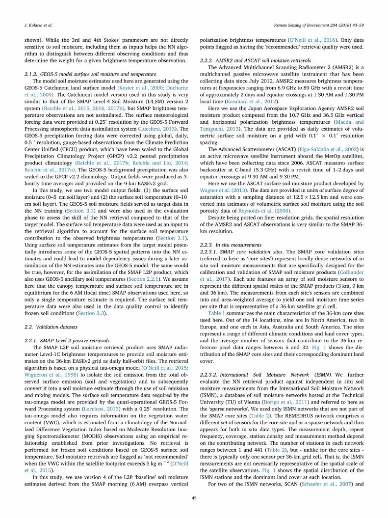
The NN and L2P retrieval products show a generally good agree-ment of the fractional error spatial patterns, but differences in the ab-solute values exist (Fig. 10). For example, the L2P retrievals tend tohave lower fractional errors (or noise-to-signal ratios) in the arid re-gions of Central Australia, the Kalahari or the Southern Sahara, possiblyindicating that the ancillary soil data used by the L2P algorithm allowsit to better account for the effect of surface roughness, which can besignificant in arid regions. However, this behavior is not observed inother arid areas, such as the Central Sahara or the Arabian Peninsula.The NN retrievals have a lower fractional error in moderately to denselyvegetated regions and transition zones, such as India, Central Africa,Eastern Brazil and Northern Australia. This suggests that in these re-gions, the NN method can produce soil moisture estimates with a highercertainty and could be used to supplement or improve the L2P re-trievals. However, due to the lack of in situ stations in these areas, thisfinding cannot be further corroborated.

While the characterization of the global error distributions is in-formative, it is important to keep in mind that the error estimates de-rived from the TC analysis here are also subject to uncertainties. Theseare related to (1) differences in the overpass times between AMSR2 andASCAT relative to SMAP and the simulation times of the model, (2) theslightly lower emission depth of the higher frequency AMSR2 andASCAT data compared to SMAP and the depth of the model's surfacelayer, and (3) potential errors in the porosity data used to convert theASCAT data into volumetric surface soil moisture estimates.

5. Summary

In this study we developed and evaluated a NN based retrieval al-gorithm to estimate global surface soil moisture from SMAP brightnesstemperatures. The SMAP NN retrieval product was trained on GEOS-5model estimates and evaluated against in situ measurements from theSMAP core validation sites and the ISMN. The skill of the NN retrievalwas compared against that of the GEOS-5 estimates and the SMAP L2Pretrievals.

The comparison of the SMAP NN retrieval product against theGEOS-5 model soil moisture showed that globally the two datasetsagree well. Differences occur in mountainous regions, where the mi-crowave satellite retrievals are uncertain, and in agricultural areas,where the satellite retrieval product possibly captures the result ofagricultural practices (such as irrigation, tilling and harvesting) that arenot represented in the model. Combined with the generally higher skillof the SMAP retrievals against in situ measurements, the results confirmthe potential for the SMAP observations to inform a model through dataassimilation, as has been shown with the SMAP Level-4 products(Reichle et al., 2017b).

The SMAP NN soil moisture estimates compare favorably againstthe SMAP core site in situ measurements with an average correlationand anomaly correlation of 0.70 and 0.66, respectively, and an averageubRMSE of 0.037 m3m−3. Evaluated against ISMN sparse network insitu measurements, the correlation and anomaly correlation were 0.58and 0.48, respectively, and the ubRMSE was 0.026 m3m−3. The coresite data better represent the spatial scales of a satellite footprint ormodel grid cell, leading to the higher skill of the NN retrieval againstcore site data than against ISMN data.

0

0.02

0.04

0.06

ubR

MS

E [m

3 m

-3]

ubRMSE

DAHRA FM

I

PBO H2O

REMEDHUS

RSMN

SMOSM

ANIA

SNOTEL

SOILSCAPE

iRON

SCAN

USCRN All

SMAP NN GEOS-5 SMAP L2P

S L E

0

0.2

0.4

0.6

0.8

1

anom

aly

corr

elat

ion

[-]

0

0.2

0.4

0.6

0.8

1

corr

elat

ion

[-]

(a)

(b)

(c)

SMAP NN GEOS-5 SMAP L2P

Fig. 7. Network average (a) correlation, (b) anomaly correlation and (c) ubRMSE between the ISMN in situ observations and the SMAP NN retrievals (red squares), the SMAP L2Pretrievals (green circles) and the GEOS-5 model soil moisture (blue diamonds). Shown are the metrics for each network as well as the average across all networks. All averages are cluster-based (Section 3.2) The error bars represent the 95% confidence interval.

J. Kolassa et al. Remote Sensing of Environment 204 (2018) 43–59

54

The NN retrievals had a higher correlation (by 0.06) and a higheranomaly correlation (by 0.09) against core site in situ measurementsthan the GEOS-5 model estimates, which were used as the NN targetdata. The corresponding average ubRMSE of the NN retrievals was0.004 m3m−3 lower than that of the GEOS-5 estimates. Evaluatedagainst ISMN data, the relative skill of the NN retrievals and modelestimates was comparable to that found during the core site evaluation.

Overall, the results suggest that (1) the NN retrievals are able to usethe SMAP brightness temperatures to correct potential errors in themodel-based target data and (2) the NN retrievals capture soil moistureinformation not present in the model, resulting in better agreementwith the core site and ISMN in situ measurements. The latter indicatesthat the NN retrievals may be beneficial in data assimilation, in parti-cular for the short-term soil moisture variations (captured by theanomaly correlations against the cores sites) for which the skill differ-ence between the retrievals and the model estimates is the highest.

Generally, the (anomaly) correlation skill of the NN retrievalsagainst core site measurements is lower than that of the SMAP L2Pproduct (by 0.08 and 0.05 for the correlations and anomaly correla-tions, respectively). The ubRMSE of the NN retrievals, however, islower than that of the L2P retrievals by 0.004 m3m−3. Evaluatedagainst ISMN data, which represent a more diverse set of local condi-tions but only provide point-scale information, the NN and L2P

retrievals have a very similar (anomaly) correlation skill, but the NNretrievals have a lower ubRMSE (by 0.04 m3m−3) than the L2P re-trievals. The slightly lower (anomaly) correlation skill of the NN re-trievals at the core sites is most likely related to errors in the trainingtarget data or missing information in the input data, whereas the higherubRMSE of the L2P retrieval at the core sites is likely related to thehigher time series variability of this product.

A triple collocation analysis using AMSR2 and ASCAT soil moistureretrievals as the additional two datasets showed that at the global scaleall three products have comparable errors relative to their respectivesoil moisture dynamic range. The NN and L2P retrieval products havevery similar error spatial patterns, but the NN retrievals have a betterskill than the L2P product in densely vegetated regions and transitionzones outside of CONUS. The GEOS-5 model has a slightly differenterror spatial patterns compared to the retrievals, with notable differ-ences in high latitudes, where the model has higher errors owing to theincreased uncertainty in its precipitation forcing, and in densely vege-tated areas, where the retrieval products are less reliable owing to thelower soil moisture sensitivity of SMAP brightness temperatures in thepresence of dense vegetation.

Overall, the skill of the SMAP NN retrievals is only slightly worsethat of the SMAP L2P retrieval product, but the NN retrievals are pro-vided in the global climatology of the GEOS-5 model, which may reduce

-120 -110 -100 -90 -80 -7025

30

35

40

45

-120 -110 -100 -90 -80 -7025

30

35

40

45

-120 -110 -100 -90 -80 -7025

30

35

40

45

Latit

ude

[deg

]

Longitude [deg]

(a) R

(b) Ranom

(c) ubRMSE

SMAP NN GEOS-5 SMAP L2PFig. 8. Skill ranking in terms of (a) correlation, (b) anomalycorrelation and (c) ubRMSE of the SMAP NN retrievals (redsquares), the GEOS-5 model soil moisture (blue diamonds) andthe SMAP L2P retrievals (green circles) at the ISMN stationslocated in the US. Each marker indicates the dataset that ob-tained the highest skill at a given station. The contributingnetworks are iRON, PBO H2O, SCAN, SNOTEL, SOILSCAPE andUSCRN.

J. Kolassa et al. Remote Sensing of Environment 204 (2018) 43–59

55

the need for further bias correction before data assimilation. Localbiases between the NN retrievals and the model, however, are retainedin the NN retrievals, which would violate typical data assimilation re-quirements. Additionally, local discrepancies between the dynamicrange of the NN retrievals and the model estimates could result in non-orthogonal errors between the observations and the model estimates,which would also violate typical data assimilation requirements.Consequently, further investigation is needed to determine the impact

of such violations on the quality of the hydrological fields and surfaceflux estimates obtained from data assimilation, and whether the as-similation system can use NN retrievals more efficiently than standardretrievals or brightness temperatures.

The natural next step is thus to assimilate the SMAP NN retrievalproduct and compare the resulting analysis skill against that of assim-ilation experiments using traditional localized or other non-localizedbias correction techniques, and against the assimilation of L2P

Longitude [deg]

Latit

ude

[deg

]

(a) SMAP NN

(b) GEOS-5

(c) SMAP L2P

Fig. 9. Fractional error standard deviations estimated fromTC for the (a) SMAP NN retrieval product, (b) GEOS-5modeled soil moisture and (c) SMAP L2P retrieval product.

J. Kolassa et al. Remote Sensing of Environment 204 (2018) 43–59

56

retrievals and brightness temperatures. Another possible extension tothis study would be to use the higher-resolution SMAP Enhanced Level-1C brightness temperature product (Chaubell et al., 2016) to generateSMAP NN soil moisture retrievals at a higher spatial resolution.

Acknowledgments

J. Kolassa was supported by the NASA Postdoctoral Program, ad-ministered by Universities Space Research Association under contractwith NASA. Additional funding was provided by the NASA SoilMoisture Active Passive mission. P. Gentine was supported by grantNNX15AB30G. Computational resources for this study were providedby the NASA High-End Computing (HEC) Program through the NASACenter for Climate Simulation (NCCS) at the Goddard Space FlightCenter. We thank Aaron Berg, Tracy Rowlandson and Erica Tetlock forproviding soil moisture measurements from the Kenaston network,which is funded by Environment and Climate Change Canada and theCanadian Space Agency. We also thank Mark Seyfried and Rogier vander Velde for providing soil moisture measurements from the ReynoldsCreek and Twente networks, respectively.

References

Aires, F., Prigent, C., Rossow, W.B., 2005. Sensitivity of satellite microwave and infraredobservations to soil moisture at a global scale: 2. Global statistical relationships. J.Geophys. Res. 110, D11103. http://dx.doi.org/10.1029/2004JD005094.

Al Bitar, A., Leroux, D., Kerr, Y.H., Merlin, O., Richaume, P., Sahoo, A., Wood, E.F., 2012.Evaluation of SMOS soil moisture products over continental US using the SCAN/SNOTEL network. IEEE Trans. Geosci. Remote Sens. 50 (5), 1572–1586. http://dx.doi.org/10.1109/TGRS.2012.2186581.

Albergel, C., Dorigo, W., Reichle, R.H., Balsamo, G., De Rosnay, P., Mu noz Sabater, J.,Isaksen, L., De Jeu, R., Wagner, W., 2013. Skill and global trend analysis of soilmoisture from reanalyses and microwave remote sensing. J. Hydrometeorol. 14 (4),1259–1277. http://dx.doi.org/10.1175/JHM-D-12-0161.1. Vancouver.

Alemohammad, S.H., Fang, B., Konings, A.G., Green, J.K., Kolassa, J., Prigent, C., Aires,F., Miralles, D., Gentine, P., 2017. Water, energy and carbon with artificial neuralnetworks (WECANN): a statistically-based estimate of global surface turbulent fluxesusing solar-induced fluorescence. Biogeosci. Discuss. http://dx.doi.org/10.5194/bg-2016-495.

Assouline, S., 2013. Infiltration into soils: conceptual approaches and solutions. WaterResour. Res. 49 (4), 1755–1772. http://dx.doi.org/10.1002/wrcr.20155.

Bateni, S.M., Entekhabi, D., 2012. Relative efficiency of land surface energy balancecomponents. Water Resour. Res. 48 (4). http://dx.doi.org/10.1029/2011WR011357.

Belward, A.S., Estes, J.E., Kline, K.D., 1999. The IGBP-DIS global 1-km land-cover data setDISCover: a project overview. Photogramm. Eng. Remote. Sens. 65 (9), 1013–1020.

Brodzik, M.J., Billingsley, B., Haran, T., Raup, B., Savoie, M.H., 2012. EASE-grid 2.0:incremental but significant improvements for Earth-gridded data sets. ISPRS Int. J.Geo-Inf. 1 (1), 32–45. http://dx.doi.org/10.3390/ijgi1010032.

Calvet, J.C., Fritz, N., Froissard, F., Suquia, D., Petitpa, A., Piguet, B., 2007. in situ soilmoisture observations for the CAL/VAL of SMOS: the SMOSMANIA network. In:Geoscience and Remote Sensing Symposium, 2007. IGARSS 2007. IEEE International(pp. 1196-1199). IEEE.

Chai, S.S., Walker, J.P., Makarynskyy, O., Kuhn, M., Veenendaal, B., West, G., 2009. Useof soil moisture variability in artificial neural network retrieval of soil moisture.Remote Sens. 2 (1), 166–190. http://dx.doi.org/10.3390/rs2010166.

Chan, S.K., Bindlish, R., O’Neill, P.E., Njoku, E., Jackson, T., Colliander, A., Chen, F.,Burgin, M., Dunbar, S., Piepmeier, J., Yueh, S., 2016b. Assessment of the SMAPpassive soil moisture product. IEEE Trans. Geosci. Remote Sens. 54 (8), 4994–5007.http://dx.doi.org/10.1109/TGRS.2016.2561938.

Chan, S., Njoku, E.G., Colliander, A., 2016. SMAP L1c Radiometer Half-Orbit 36 KmEASE-Grid Brightness Temperatures, Version 3. Boulder, Colorado USA. NASANational Snow and Ice Data Center Distributed Active Archive Centerhttp://dx.doi.org/10.5067/E51BSP6V3KP7.

Chaubell, M.J., Chan, S., Dunbar, R.S., Peng, J., Yueh, S., 2016. SMAP Enhanced L1CRadiometer Half-Orbit 9 Km EASE-Grid Brightness Temperatures Version 1. Boulder,Colorado USA. NASA National Snow and Ice Data Center Distributed Active ArchiveCenterhttp://dx.doi.org/10.5067/2C9O9KT6JAWS.

Chen, F., Crow, W.T., Colliander, A., Cosh, M.H., Jackson, T.J., Bindlish, R., Reichle, R.H.,Chan, S.K., Bosch, D.D., Starks, P.J., Goodrich, D.C., 2017. Application of triplecollocation in ground-based validation of Soil Moisture Active/Passive (SMAP) level2 data products. IEEE Journal of Selected Topics in Applied Earth Observations andRemote Sensing 10 (2), 489–502.

Colliander, A., Jackson, T.J., Bindlish, R., Chan, S., Das, N., Kim, S.B., Cosh, M.H.,Dunbar, R.S., Dang, L., Pashaian, L., Asanuma, J., 2017. Validation of SMAP surfacesoil moisture products with core validation sites. Remote Sens. Environ. 191,215–231.

Corradini, C., Morbidelli, R., Melone, F., 1998. On the interaction between infiltrationand Hortonian runoff. J. Hydrol. 204 (1), 52–67. http://dx.doi.org/10.1016/S0022-1694(97)00100-5.

Cybenko, G.V., 1989. Approximation by superpositions of a sigmoidal function,Mathematics of Control. Signals Syst. 2, 303–314. http://dx.doi.org/10.1007/BF02551274.

De Lannoy, G.J., Koster, R.D., Reichle, R.H., Mahanama, S.P., Liu, Q., 2014. An updatedtreatment of soil texture and associated hydraulic properties in a global land mod-eling system. J. Adv. Model. Earth Syst. 6 (4), 957–979. http://dx.doi.org/10.1002/2014MS000330.

De Lannoy, G.J., Reichle, R.H., 2016. Global assimilation of multiangle and multi-polarization SMOS brightness temperature observations into the GEOS-5 catchmentland surface model for soil moisture estimation. J. Hydrometeorol. 17 (2), 669–691.http://dx.doi.org/10.1175/JHM-D-15-0037.1.

De Lannoy, G.J.M., Reichle, R.H., Peng, J., Kerr, Y., Castro, R., Kim, E.J., Liu, Q., 2015.Converting between SMOS and SMAP level-1 brightness temperature observationsover nonfrozen land. IEEE Geosci. Remote Sens. Lett. 12, 1908–1912. http://dx.doi.org/10.1109/LGRS.2015.2437612.

Diamond, H.J., Karl, T.R., Palecki, M.A., Baker, C.B., Bell, J.E., Leeper, R.D., Easterling,D.R., Lawrimore, J.H., Meyers, T.P., Helfert, M.R., Goodge, G., 2013. US climatereference network after one decade of operations: status and assessment. Bull. Am.Meteorol. Soc. 94 (4), 485–498. http://dx.doi.org/10.1175/BAMS-D-12-00170.1.

Dorigo, W.A., Wagner, W., Hohensinn, R., Hahn, S., Paulik, C., Xaver, A., Gruber, A.,Drusch, M., Mecklenburg, S., van Oevelen, P., Robock, A., Jackson, T., 2011. TheInternational Soil Moisture Network: a data hosting facility for global in situ soilmoisture measurements. Hydrol. Earth Syst. Sci. 15, 1675–1698. http://dx.doi.org/10.5194/hess-15-1675-2011.

Longitude [deg]

Latit

ude

[deg

]

Fig. 10. Difference of the fractional error standard devia-tions between the NN and L2P retrievals (NN - L2P).Negative values (red) indicate a lower fractional error andhigher signal-to-noise ratio for the NN retrievals and posi-tive values (blue) indicate a lower fractional error of theL2P retrievals.

J. Kolassa et al. Remote Sensing of Environment 204 (2018) 43–59

57

Draper, C.S., Reichle, R., de Jeu, R., Naeimi, V., Parinussa, R., Wagner, W., 2013.Estimating root mean square errors in remotely sensed soil moisture over continentalscale domains. Remote Sens. Environ. 137, 288–298. http://dx.doi.org/10.1016/j.rse.2013.06.013.

Ducharne, A., Koster, R.D., Suarez, M.J., Stieglitz, M., Kumar, P., 2000. A catchment-based approach to modeling land surface processes in a general circulation model: 2.Parameter estimation and model demonstration. J. Geophys. Res. 105 (24), 823–824.http://dx.doi.org/10.1029/2000JD900328.

Entekhabi, D., Nakamura, H., Njoku, E.G., 1994. Solving the inverse problem for soilmoisture and temperature profiles by sequential assimilation of multifrequency re-motely sensed observations. IEEE Trans. Geosci. Remote Sens. 32 (2), 438–448.http://dx.doi.org/10.1109/36.295058.

Entekhabi, D., Njoku, E.G., O’Neill, P.E., Kellogg, K.H., Crow, W.T., Edelstein, W.N., 2010.The soil moisture active passive (SMAP) mission. Proc. IEEE 98 (5), 704–716. http://dx.doi.org/10.1109/JPROC.2010.2043918.

Figa-Saldaña, J., Wilson, J.J., Attema, E., Gelsthorpe, R., Drinkwater, M.R., Stoffelen, A.,2002. The advanced scatterometer (ASCAT) on the meteorological operational(MetOp) platform: a follow on for European wind scatterometers. Can. J. Remote.Sens. 28 (3), 404–412. http://dx.doi.org/10.5589/m02-035.

Gentine, P., Polcher, J., Entekhabi, D., 2011. Harmonic propagation of variability insurface energy balance within a coupled soil-vegetation-atmosphere system. WaterResour. Res. 47 (5). http://dx.doi.org/10.1029/2010WR009268.

Gruber, A., Su, C.H., Zwieback, S., Crow, W., Dorigo, W., Wagner, W., 2016. Recentadvances in (soil moisture) triple collocation analysis. Int. J. Appl. Earth Obs. Geoinf.45, 200–211. http://dx.doi.org/10.1016/j.jag.2015.09.002.

Jimenez, C., Clark, D.B., Kolassa, J., Aires, F., Prigent, C., 2013. A joint analysis ofmodeled soil moisture fields and satellite observations. J. Geophys. Res 118 (12),6771–6782. http://dx.doi.org/10.1002/jgrd.50430.

Jung, M., Reichstein, M., Schwalm, C.R., Huntingford, C., Sitch, S., Ahlström, A., Arneth,A., Camps-Valls, G., Ciais, P., Friedlingstein, P., Gans, F., 2017. Compensatory watereffects link yearly global land CO2 sink changes to temperature. Nature 541 (7638),516–520. http://dx.doi.org/10.1038/nature20780.

Kasahara, M., Imaoka, K., Kachi, M., Fujii, H., Naoki, K., Maeda, T., Ito, N., Nakagawa, K.,Oki, T., 2012. Status of AMSR2 on GCOM-w1. In: SPIE Remote Sensing. InternationalSociety for Optics and Photonics. http://proceedings.spiedigitallibrary.org/pdfaccess.ashx?url=/data/conferences/spiep/69394/853307.pdf 853307–853307.

Kerr, Y.H., Waldteufel, P., Richaume, P., Wigneron, J.P., Ferrazzoli, P., Mahmoodi, A., AlBitar, A., Cabot, F., Gruhier, C., Juglea, S.E., Leroux, D., 2012. The SMOS soilmoisture retrieval algorithm. IEEE Trans. Geosci. Remote Sens. 50 (5), 1384–1403.http://dx.doi.org/10.1109/TGRS.2012.2184548.

Kerr, Y.H., Waldteufel, P., Wigneron, J.P., Delwart, S., Cabot, F., Boutin, J., Escorihuela,M.J., Font, J., Reul, N., Gruhier, C., Juglea, S.E., Drinkwater, M.R., Hahne, A., Martin-Neira, M., Mecklenburg, S., 2010. The SMOS mission: new tool for monitoring keyelements of the global water cycle. Proc. IEEE 98 (5), 666–687. http://dx.doi.org/10.1109/JPROC.2010.2043032.

Kolassa, J., 2013. Soil moisture retrieval from multi-instrument satellite observations. In:Doctoral Dissertation. Université Pierre et Marie Curie (Paris 6). http://www.theses.fr/2013PA066392.

Kolassa, J., Aires, F., Polcher, J., Prigent, C., Jimenez, C., Pereira, J.M., 2013. Soilmoisture retrieval from multi-instrument observations: information content analysisand retrieval methodology. J. Geophys. Res 118 (10), 4847–4859. http://dx.doi.org/10.1029/2012JD018150.

Kolassa, J., Gentine, P., Prigent, C., Aires, F., 2016. Soil moisture retrieval from AMSR-eand ASCAT microwave observation synergy. Part 1: Satellite data analysis. RemoteSens. Environ. 173, 1–14. http://dx.doi.org/10.1016/j.rse.2015.11.011.

Koster, R.D., Suarez, M.J., Ducharne, A., Stieglitz, M., Kumar, P., 2000. A catchment-based approach to modeling land surface processes in a general circulation model: 1.Model structure. J. Geophys. Res. Atmos. 105 (D20), 24809–24822. http://dx.doi.org/10.1029/2000JD900327.

Lahoz, W.A., De Lannoy, G.J., 2014. Closing the gaps in our knowledge of the hydro-logical cycle over land: conceptual problems. Surv. Geophys. 35 (3), 623–660. http://dx.doi.org/10.1007/s10712-013-9221-7.

Larson, K.M., Small, E.E., Gutmann, E.D., Bilich, A.L., Braun, J.J., Zavorotny, V.U., 2008.Use of GPS receivers as a soil moisture network for water cycle studies. Geophys. Res.Lett. 35 (24). http://dx.doi.org/10.1029/2008GL036013.

Leavesley, G.H., David, O., Garen, D.C., Lea, J., Marron, J.K., Pagano, T.C., Perkins, T.R.,Strobel, M.L., 2008. A modeling framework for improved agricultural water supplyforecasting. In: AGU Fall Meeting Abstracts.

Levenberg, K., 1944. A method for the solution of certain non-linear problems in leastsquares. Q. Appl. Math. 2 (2), 164–168.

Liu, Q., Reichle, R.H., Bindlish, R., Cosh, M.H., Crow, W.T., de Jeu, R., De Lannoy, G.J.,Huffman, G.J., Jackson, T.J., 2011. The contributions of precipitation and soilmoisture observations to the skill of soil moisture estimates in a land data assimila-tion system. J. Hydrometeorol. 12 (5), 750–765. http://dx.doi.org/10.1175/JHM-D-10-05000.1.

Lucchesi, R., 2013. File Specification for GEOS-5 FP. NASA Global Modeling andAssimilation Office (GMAO) Office Note No. 4 (Version 1.0), pp. 63.

Maeda, T., Taniguchi, Y., 2013. Descriptions of GCOM-W1 AMSR2 Level 1R and Level 2Algorithms. Japan Aerospace Exploration Agency Earth Observation Research Center,Ibaraki, Japan. suzaku.eorc.jaxa.jp/GCOM_W/data/doc/NDX-120015A.pdf.

Marquardt, D.W., 1963. An algorithm for least-squares estimation of nonlinear para-meters. J. Soc. Ind. Appl. Math. 11 (2), 431–441. http://dx.doi.org/10.1137/0111030.

McColl, K.A., Vogelzang, J., Konings, A.G., Entekhabi, D., Piles, M., Stoffelen, A., 2014.Extended triple collocation: estimating errors and correlation coefficients with re-spect to an unknown target. Geophys. Res. Lett. 41 (17), 6229–6236. http://dx.doi.

org/10.1002/2014GL061322.McDowell, N.G., 2011. Mechanisms linking drought, hydraulics, carbon metabolism, and

vegetation mortality. Plant Physiol. 155 (3), 1051–1059. http://dx.doi.org/10.1104/pp.110.170704.

Moghaddam, M., Silva, A.R., Clewley, D., Akbar, R., Hussaini, S.A., Whitcomb, J.,Devarakonda, R., Shrestha, R., Cook, R.B., Prakash, G., Vannan, S.S., 2016. SoilMoisture Profiles and Temperature Data from SoilSCAPE Sites, USA. ORNL DAACOak Ridge. Tennessee, USA. http://dx.doi.org/10.3334/ORNLDAAC/1339.

O’Neill, P., Chan, S., Njoku, E., Jackson, T., Bindlish, R., 2015. SMAP algorithm theore-tical basis document: L2 & l3 radiometer soil moisture (passive) products. In: SMAPProject, JPL D-66480. Jet Propulsion Laboratory, Pasadena, CA. https://nsidc.org/sites/nsidc.org/files/technical-references/L2_SM_P_ATBD_v7_Sep2015-po-en.pdf.

O’Neill, P.E., Chan, S., Njoku, E.G., Jackson, T., Bindlish, R., 2016. SMAP L2 RadiometerHalf-Orbit 36 Km EASE-Grid Soil Moisture, Version 3. Boulder, Colorado USA.National Snow and Ice Data Center Distributed Active Archive Centerhttp://dx.doi.org/10.5067/PLRS64IU03IT. Accessed: June 2016.

Owe, M., deJeu, R., Walker, J., 2001. A methodology for surface soil moisture and ve-getation optical depth retrieval using the microwave polarization difference index.IEEE Trans. Geosci. Remote Sens. 39, 1643–1654. http://dx.doi.org/10.1109/36.942542.

Philip, J.R., 1957. The theory of infiltration: 5. The influence of the initial moisturecontent. Soil Sci. 84 (4), 329–340.

Reichle, R.H., Lannoy, G.J.M.D.e., Liu, Q., Colliander, A., Conaty, A., Jackson, T.,Kimball, J., Koster, R.D., 2015. Soil moisture active passive (SMAP) project assess-ment report for the beta-release l4_SM data product. In: NASA Technical ReportSeries on Global Modeling and Data Assimilation, NASA/TM-2015-104606, Vol. 40,National Aeronautics and Space Administration. Goddard Space Flight Center,Greenbelt, Maryland, USA, pp. 63. Available at: https://gmao.gsfc.nasa.gov/pubs/.

Reichle, R.H., De Lannoy, G.J., Liu, Q., Ardizzone, J.V., Chen, F., Colliander, A., Conaty,A., Crow, W., Jackson, T., Kimball, J., Koster, R.D., 2016. Soil moisture active passivemission l4_SM data product assessment (version 2 validated release). In: NASA GlobalModelling and Assimilation Office (GMAO) Office Note No. 12, . https://nsidc.org/sites/nsidc.org/files/technical-references/Reichle851.pdf.

Reichle, R.H., De Lannoy, G.J., Liu, Q., Ardizzone, J.V., Colliander, A., Conaty, A., Crow,W., Jackson, T.J., Jones, L.A., Kimball, J.S., Koster, R.D., 2017b. Assessment of theSMAP Level-4 Surface and Root-Zone Soil Moisture Product Using In SituMeasurements. J. Hydrometeorol. 18 (10), 2621–2645. http://dx.doi.org/10.1175/JHM-D-17-0063.1.

Reichle, R.H., De Lannoy, G.J., Liu, Q., Colliander, A., Conaty, A., Jackson, T., Kimball, J.,Koster, R.D., 2015b. Soil moisture active passive (SMAP) project assessment reportfor the beta-release l4_SM data product. In: NASA Technical Report Series on GlobalModeling and Data Assimilation. 104606. NASA/TM-2015, pp. 40–63. https://nsidc.org/sites/nsidc.org/files/technical-references/Reichle788.pdf.

Reichle, R.H., Koster, R.D., 2004. Bias reduction in short records of satellite soil moisture.Geophys. Res. Lett. 31, L19501. http://dx.doi.org/10.1029/2004GL020938.

Reichle, R.H., Liu, Q., 2014. Observation-Corrected Precipitation Estimates in GEOS-5.35 NASA/TM 2014-104606 doi: 20150000725.

Reichle, R.H., Liu, Q., Koster, R.D., Draper, C.S., Mahanama, S.P., Partyka, G.S., 2017a.Land surface precipitation in MERRA-2. J. Clim. 30, 1643–1664. http://dx.doi.org/10.1175/JCLI-D-16-0570.1.

Reynolds, C.A., Jackson, T.J., Rawls, W.J., 2000. Estimating soil water-holding capacitiesby linking the Food and Agriculture Organization soil map of the world with globalpedon databases and continuous pedotransfer functions. Water Resour. Res. 36 (12),3653–3662. http://dx.doi.org/10.1029/2000WR900130.

Rodríguez-Fernández, N.J., Aires, F., Richaume, P., Kerr, Y.H., Prigent, C., Kolassa, J.,Cabot, F., Jiménez, C., Mahmoodi, A., Drusch, M., 2015. Soil moisture retrieval usingneural networks: application to SMOS. IEEE Trans. Geosci. Remote Sens. 53 (11),5991–6007. http://dx.doi.org/10.1109/TGRS.2015.2430845.

Rumelhart, D.E., Chauvin, Y., 1995. Backpropagation: Theory, Architectures, andApplications. Lawrence Erlbaum Associates ISBN: 0-8058-1258-X.

Sanchez, N., Martínez-Fernández, J., Scaini, A., Perez-Gutierrez, C., 2012. Validation ofthe SMOS L2 soil moisture data in the REMEDHUS network (Spain). IEEE Trans.Geosci. Remote Sens. 50 (5), 1602–1611. http://dx.doi.org/10.1109/TGRS.2012.2186971.

Santi, E., Paloscia, S., Pettinato, S., Fontanelli, G., 2016. Application of artificial neuralnetworks for the soil moisture retrieval from active and passive microwave space-borne sensors. Int. J. Appl. Earth Obs. Geoinf. 48, 61–73. http://dx.doi.org/10.1016/j.jag.2015.08.002.

Schaefer, G.L., Cosh, M.H., Jackson, T.J., 2007. The USDA natural resources conservationservice soil climate analysis network (SCAN). J. Atmos. Ocean. Technol. 24 (12),2073–2077. http://dx.doi.org/10.1175/2007JTECHA930.1.

Schmugge, T.J., Jackson, T.J., McKim, H.L., 1980. Survey of methods for soil moisturedetermination. Water Resour. Res. 16 (6), 961–979.

Scipal, K., Holmes, T., De Jeu, R., Naeimi, V., Wagner, W., 2008. A possible solution forthe problem of estimating the error structure of global soil moisture data sets.Geophys. Res. Lett. 35 (24). http://dx.doi.org/10.1029/2008GL035599.

Seneviratne, S.I., Lüthi, D., Litschi, M., Schär, C., 2006. Land-atmosphere coupling andclimate change in Europe. Nature 443 (7108), 205–209. http://dx.doi.org/10.1038/nature05095.

Sevanto, S., McDowell, N.G., Dickman, L.T., Pangle, R., Pockman, W.T., 2014. How dotrees die? A test of the hydraulic failure and carbon starvation hypotheses. Plant CellEnviron. 37 (1), 153–161. http://dx.doi.org/10.1111/pce.12141.

Stoffelen, A., 1998. Toward the true near-surface wind speed: error modeling and cali-bration using triple collocation. J. Geophys. Res. 103 (C4), 7755–7766. http://dx.doi.org/10.1029/97JC03180.

Su, C.H., Ryu, D., Crow, W.T., Western, A.W., 2014. Beyond triple collocation:

J. Kolassa et al. Remote Sensing of Environment 204 (2018) 43–59

58

applications to soil moisture monitoring. J. Geophys. Res. Atmos. 119 (11),6419–6439. http://dx.doi.org/10.1002/2013JD021043.

World Meteorological Organization - Global Climate Observing System, 2009. Guidelinefor the generation of satellite-based datasets and products meeting GCOS require-ments. WMO technical document 1488. https://public.wmo.int/en/programmes/global-climate-observing-system/Publications/gcos-143.pdf.

Tagesson, T., Fensholt, R., Guiro, I., Rasmussen, M.O., Huber, S., Mbow, C., Garcia, M.,Horion, S., Sandholt, I., Holm?Rasmussen, B., Göttsche, F.M., 2015. Ecosystemproperties of semiarid savanna grassland in west Africa and its relationship withenvironmental variability. Glob. Chang. Biol. 21 (1), 250–264. http://dx.doi.org/10.1111/gcb.12734.

Taylor, J.R., Osenga, E.C., Jack-Scott, E., Arnott, J.C., Katzenberger, J., 2015. Establishinga Long Term High-Altitude Soil Moisture Monitoring Network at the Watershed Scale.

AGU Fall Meeting Abstracts.Wagner, W., Hahn, S., Kidd, R., Melzer, T., Bartalis, Z., Hasenauer, S., Rubel, F., 2013. The

ASCAT soil moisture product: a review of its specifications, validation results, andemerging applications. Meteorol. Z 22 (1), 5–33. http://dx.doi.org/10.1127/0941-2948/2013/0399.

Walker, J.P., Houser, P.R., 2001. A methodology for initializing soil moisture in a globalclimate model: assimilation of near-surface soil moisture observations. J. Geophys.Res. 106 (D11), 11761–11774. http://dx.doi.org/10.1029/2001JD900149.

Wigneron, J.P., Chanzy, A., Calvet, J.C., Bruguier, N., 1995. A simple algorithm to re-trieve soil moisture and vegetation biomass using passive microwave measurementsover crop fields. Remote Sens. Environ. 51 (3), 331–341. http://dx.doi.org/10.1016/0034-4257(94)00081-W.

J. Kolassa et al. Remote Sensing of Environment 204 (2018) 43–59

59