Remote Sensing of Environment - USGS & Javier Gallego, 2005; Hanuschak et al., 2001; Wardlow & Egbert, 2008). ... data and Monte Carlo simulation. Their results suggest that the

Remote Sensing of Environment 114 (2010) 1190–1204

Contents lists available at ScienceDirect

Remote Sensing of Environment

j ourna l homepage: www.e lsev ie r.com/ locate / rse

The spatial distribution of crop types from MODIS data: Temporal unmixing usingIndependent Component Analysis

Mutlu OzdoganCenter for Sustainability and the Global Environment (SAGE) 1710 University Avenue Madison, WI 53726, USA

E-mail address: [email protected].

0034-4257/$ – see front matter © 2010 Elsevier Inc. Aldoi:10.1016/j.rse.2010.01.006

a b s t r a c t
a r t i c l e i n f o
Article history:Received 6 September 2009Received in revised form 26 December 2009Accepted 9 January 2010

Keywords:AgricultureICAUnmixingMODISCropsWheatTurkey

Remote sensing plays an important role in delivering accurate and timely information on the location and areaof major crop types with important environmental, economic, and policy considerations. The purpose of thispaper is to report on an unsupervised signal processing algorithm called Independent Component Analysis(ICA) to temporally decompose MODerate-resolution Imaging Spectroradiometer (MODIS) data toautomatically map major crop types in three agricultural regions covering parts of Kansas and Nebraska inthe US and a third in northwestern Turkey. The approach proposed here is based on the premise that thetemporal profiles of individual crops are observed as mixtures with a moderate-resolution sensor whencultivated fields are smaller than the spatial resolution of the observing sensor. The purpose of ICA is todecompose these mixed observations by a remote sensor into individual crop signals, using only the mixedobservations without the aid of information about the crop signatures and the mixing process. Results usingboth synthetic data and real observations suggest that the ICA approach can successfully separate generalized,landscape-level cropping patterns using only available temporalmeasurements. There is very little need to usecomplicated indices or derivative spectral products to map crop types using ICA: availability of high temporalobservations, either as raw spectral bands or simple vegetation indices is sufficient to identify crop types at thescale of landscapes. Results also suggest that crop map predictions aggregated to coarser resolutions havebetter accuracy than at native resolution when compared to maps made from fine-scale observations used asground truth. These accuracies range from RMSE of 15–30% at 500 m to less than 10% at 2000 m. The success ofthe initial results presented here to automaticallymap crop distributions across large areas usingMODIS data isparticularly encouraging given the existing and planned worldwide observations of agriculturally importantregions. However, the use of ICA for operational crop monitoring will require algorithms that will take intoaccount prior information on crop growth curves, constrained estimation of independent components, andscaling of mixing vectors to obtain physically possible ranges.

l rights reserved.

© 2010 Elsevier Inc. All rights reserved.

1. Introduction

Accurate and timely information on the location and area of majorcrop types has significant economic, food, policy, and environmentalimplications. For example, annual crop production data from differentparts of the globe are used to predict commodity prices (Deaton &Laroque, 1992; Nelson, 2002). Spatially disaggregated agriculturalarea and production statistics are required to distinguish patterns ortrends that are heterogeneous within countries (You et al., 2004).Policy decision makers also require information on food production tobetter assess the food aid requirements for areas affected by cropfailures (FEWSNET, 2005). Traditionally, crop acreage over large areashas been obtained with statistically-based ground surveys that arevery costly and do not provide information sufficiently detailed todetermine either the extent or the geographical distribution of major

crops. As a result, remote sensing, either alone or in combination withground surveys, has been used in crop acreage assessment (Allen, 1990;Carfagna & Javier Gallego, 2005; Hanuschak et al., 2001; Wardlow &Egbert, 2008).

Synoptic view, spatial coverage, spectral response, and the digitalnature of data are some of the advantages of using remotely sensedobservations in annual crop surveys. Suchdatapermit thepreparationofbase maps on land-use classification as well as land degradation mapsthat are spatially explicit for natural resource assessment. Vegetativephenomena associated with agriculture are dynamic due to sowing,growth, and harvest practices and remote sensing offers the ability toappraise vegetation conditions at any time essential for crop conditionand yield assessment. Thus, remote sensing and the variety of methodsto process image data represent essential tools for the enhancementof traditional agricultural management strategies.

While all dimensions of remotely sensed data are relevant, forpractical purposes it is the temporal information dimension that hasbeenmost useful for identifyingmajor crop typeswith remote sensing

mailto:[email protected]

http://dx.doi.org/10.1016/j.rse.2010.01.006

http://www.sciencedirect.com/science/journal/00344257

1191M. Ozdogan / Remote Sensing of Environment 114 (2010) 1190–1204

(Smith & Ramey, 1982; Badhwar, 1984c; Hall & Badhwar, 1987;Price et al., 1997; Wardlow et al., 2007). This is because agriculturalproducts have well established crop calendars that follow water andenergy availability. At any point during the growing season, crops areat different stages of maturity, and these stages are manifested asdifferential levels of spectral reflectance in remotely sensed signals,thereby building a crop-specific temporal record. Hence, by monitor-ing spectral indices that are sensitive to vegetation cover over time, itis possible to distinguish crops and other land-cover types.

A long list of studies has exploited the temporal nature of remotelysensed signals for crop identification. For example, Badhwar (1984a)proposed a methodology to extract crop characteristics from themulti-temporal/multi-spectral Landsat Multi-Spectral Scanner (MSS)data over large areas. Some of these characteristic features were alsopredictable from agro-meteorological models. Badhwar (1984b) alsodeveloped a crop proportion estimation method based on at least twotemporal acquisitions over the growing season, positioned at char-acteristic crop growth stages. Additionally, he proposed (1984c) amulti-temporal greenness profile applied to the Landsat MSS data toseparate corn, soybean and other ground cover classes in the US. Later,Hall and Badhwar (1987) successfully extended the temporal profilebased signatures across many geographic regions for cropmonitoring.Menenti et al. (1993) used Fourier time-series analysis to map agro-ecological zones using coarse resolution data. More recently, Vyaset al. (2005) proposed a multi-temporal crop classification in Indiathat could classify various crops in this study area regardless of date.

Despite the long history and the promise of temporalmonitoring ofcrop types however, remote sensing has not been widely operationalfor crop acreage assessment, at least not over large areas. Two reasonscontribute to this lack. First, in most places around the world, agri-culturalfields are relatively small, so they require data frommedium tohigh spatial resolution sensors, such as those provided by Landsat andSPOT (Système Pour l'Observation de la Terre) to resolve individualfields. But this spatial detail comes at the cost of reduced temporalavailability: due to predetermined acquisition strategies and obstruc-tions by clouds, only a few high spatial resolution images are usuallyavailable during critical growing periods. Even if the necessary imagedata were available, the increased number of datasets makes the costprohibitive for operational applications.Moreover,medium resolutiondata such as those provided by the Landsat systemmaybe too coarse inlocations with very small cultivated fields (e.g. China), even though inlocationswith large field sizes (e.g. USA) suchmedium resolution dataare considered “high resolution” (Ozdogan & Woodcock, 2006).

Second, there is a tradeoff between spatial detail and area cover-age. The high spatial resolution data, while providing detailed in-formation on the shapes and sizes of individual fields, cover only smallgeographical areas at a time, so that mosaics must be made frommultiple images that are often acquired at different times during thegrowing cycle of a crop. In contrast, lower spatial resolution dataprovide extensive coverage at continental and global scales, but lackthe ability to reveal specific details on the fields of interest. Thusmanyof the pixels generated by coarse resolution sensors are not char-acteristic of any one crop but relate to a mixture.

To overcome this mixed pixel issue, several investigators havedeveloped methods that utilize the concept of “temporal unmixing”(Adams et al., 1986) of high frequency observations at low spatialresolutions. Much like the traditional spectral unmixing technique,where pure endmembers are characterized by their spectral response,temporal unmixing utilizes endmembers defined by their unique tem-poral shape. The unmixingproblem then is to recover the fractional areaof each endmember based on its contribution to the mixed temporalresponse observed by the sensor. Quarmby et al. (1992) developed atechnique for estimatingcrop coverageusing linearmixturemodelingofmulti-temporal Advanced Very High Resolution Radiometer (AVHRR)data and estimated crop areas with an average accuracy of 89% ona regional scale. Kerdiles and Grondona (1995) reported on a similar

method to decompose AVHRR pixels in the Argentine Pampas to re-cover crop time profiles and crop acreage estimates with good results.Puyou-Lascassies et al. (1994) reported a regression-based approachfor unmixing coarse resolution data for crop assessment by simulatingSPOT-HRVdata. Faivre and Fischer (1997), in an important contribution,proposed a statistical modeling of coarse resolution satellite data topredict information relative to crops observed through mixed pixels.The model assumes that the reflectance of a single crop has Gaussiandistribution with parameters depending on the crop in a homogeneousagro-climatic region. The model then uses the best linear unbiasedprediction to predict the individual variations of reflectances condi-tional on the percentage of land occupation.When applied to simulatedSPOT images, the model gives good results. In a similar vein, Cherchaliet al. (2000) described a methodology for radiometrically unmixingcoarse resolution signals through the inversion of linearmixturemodel-ing on heterogeneous regions. More recently, Lobell and Asner (2004)proposed a temporal extension of the multi-endmember spectralunmixing approach, termed probabilistic temporal unmixing, whereendmember sets, and their uncertainty, are constructed using Landsatdata and Monte Carlo simulation. Their results suggest that theperformance of the mixture model varies depending on the scale ofcomparison, ranging from 50% for individual pixels to greater than 80%for crop cover across regions.

A closer look at these studies reveal that they all use a “supervised”approach tomixed pixel decompositionwhere temporal endmembersare required a priori to extract desired outputs. However, in manylocations around the world, these learning samples may not be avail-able or, even if available, may not be of good quality or be availablefor every crop type in question. An alternative approach to the tem-poral unmixing problem is to use unsupervised learning, much liketraditional unsupervised classification, where a clustering algorithmis used to extract spectral classes from image data. In the temporalcase, spectral classes become temporal classes defined by character-istic time curves, which are then interpreted by an experienced userto match crop profiles and crop area distributions. Development ofunsupervisedmethods to extract crop temporal profiles in the absenceof prior information is attractive, especially in places where thequantity and quality of learning examples are limited.

The purpose of this paper is to report on an unsupervised signaldecomposition algorithm called the Independent Component Analysis(ICA) (Comon, 1994) to unmix observed remote sensing signals in acoarse resolution pixel in order to extract the original source signals,or crop temporal signatures. Note that throughout this paper, “sourcesignals” and “crop temporal signatures” are used interchangeably. TheICA method is a special case of the Blind Source Separation (BSS)technique, which is used to separate a specific set of signals from a setof mixed observations without the aid of information about the sourcesignals or the mixing process. BSS relies on the assumption that thesource signals are completely uncorrelated and thus separates oneset of signals into a set of different signals, such that the statisticalindependence between signals is maximized. As it happens, thetemporal unmixing problem typical of crop type extraction problemslends itself nicely to the BSS approach. Our objectives here are to firstdemonstrate the temporal unmixing capabilities of the ICA methodwith a synthetic dataset to answer questions related to the effects ofinput features and scaling, and then to apply the technique to MODISvegetation index data in three distinct locations that are agriculturallyimportant. We will first provide details on the ICA algorithm, thenpresent a small numerical example using simulated data, and finallypresent results from application of ICA to real MODIS data.

2. Independent Component Analysis (ICA)

ICA is a relatively new statistical and computational techniquebased on a generativemodel,whose purpose is to reveal hidden factorsthat underlie sets of random variables, measurements, or signals that

1192 M. Ozdogan / Remote Sensing of Environment 114 (2010) 1190–1204

are assumed to be a mixture of several underlying sources called in-dependent components (Comon, 1994; Hyvärinen & Oja, 2000). Thesesource variables are also assumed to be non-Gaussian and mutuallyindependent of each other. The most attractive property of ICA is thatneither the sources nor the mixing model needs to be known. ICA issuperficially related to Principal Component Analysis (PCA) but ICA is amuch more powerful technique, capable of finding the underlyingfactors or sourceswhenPCAor factor analysis fails (Hyvärinen, 1999a).

Let N be the number of pixels in a remotely sensed image and T bethe number of images acquired over an observation period (e.g. a cropgrowing season). Let X=[xtn] be the (T×N) data matrix whose rowsare the individual images, and whose columns are the single pixelreflectance time series, or vegetation index temporal curves. TheICA model assumes that the observed data matrix X is obtained byconvolving the source matrix Swhose rows areM independent sourceimages (M×N) with the mixing matrix A (T×M) with M≤T:

X = AS: ð1Þ

For remotely sensed imagery over croplands, this notation meansthat the observed reflectance in a coarse resolution pixel (X) is amixture of several independent source signals (S) characteristic ofindividual crops grown in cultivated fields that are smaller than theinstantaneous field of view (IFOV) of an observing sensor. Here themixing matrix (A) represents the entire remote sensing convolutionprocess including the noise and themodulator transfer function (MTF)process (Markham, 1985).

It is more convenient to write the ICA model in a vector form:

xn = Asn; n = 1;…:;N ð2Þ

where xn is the T dimensional vector representing the nth pixel timecurve through all the T images over the observation period, and snis the corresponding source vector with independent components,or crop temporal curves. Once again, the linear combination of thesource vectors, sn with the mixing vector am in Eq. (3)

xn = ∑M

m=1amsmn ð3Þ

gives rise to the observed temporal profiles, xn. The mixing vector amcharacterizes the temporal behavior of the mth source, while thesource image (smn), n=1,…,N characterizes the spatial behavior of themth source over the pixel field. The ICAmodel in Eq. (3) is considered agenerative model, which describes how the observed data vector inx is generated by a process of mixing original sources in s. As such,neither the mixing matrix nor the independent components areknown and theymust be estimated from only the observation vector xunder a few general assumptions (Hyvärinen & Oja, 2000). The ICAproblem is then to solve the mixing matrix A, or more correctly itsinverse, the “unmixing” matrix W to get at the sources sn, given onlythe (mixed) observations xn:

sn = Wxn; n = 1;…:;N: ð4Þ

The two most important assumptions in the ICA generative modelare statistical independence and non-Gaussian distribution of sourcesignals. Statistically, two random variables are said to be mutuallyindependent if their probability density functions can be factorized.In cumulative distribution form, this definition leads to the mostimportant property of independent random variables defined by:

E g xð Þh yð Þf g−E g xð Þf gE h yð Þf g = 0; for i≠j ð5Þ

where g(x) and h(y) are any integrable functions of x and y. Thiscondition also distinguishes independence from uncorrelatedness

(which is a much weaker requirement) and allows the coefficients ofthemixingmatrix to be determined uniquely (Hyvärinen&Oja, 2000).

Two random variables with a joint Gaussian distribution present aspecial case where independence and uncorrelatedness are equiva-lent and this property gives rise to non-applicability of ICA forGaussian variables. In fact, the key to estimating the ICA model is ameasure of non-Gaussianality (Hyvärinen & Oja, 2000), which is oftenaccomplished by kurtosis (or the fourth-order cumulant).

A large variety of ICA methods exist for solving Eq. (4), includingstatistical or theoretical information criteria like maximum likelihoodestimation, minimization of mutual information between the sources,or maximizing the non-Gaussianality of the sources (Hyvärinen,1999a). For the temporal unmixing example presented here, we havechosen the FastICA algorithm (Hyvärinen & Oja, 2000; Hyvärinen,1999b) because of its appealing fast convergence properties, as wellas its robustness. Unlike the majority of its equivalents, the FastICAalgorithm uses negative entropy (negentropy), which is used as ameasure of (negative) distance to normality, as a non-Gaussianalitymetric using a fixed-point iteration scheme (Hyvärinen, 1999b). Theuse of negentropy in this situation is justified because in informationtheory, a Gaussian variable is said to have the largest entropy amongall random variables of equal variance (Cover & Thomas, 1991).

It is worth noting that ICA can be used in two complementaryways to decompose remotely sensed image sequences into a set ofimages and a corresponding set of time courses: Temporal ICA finds aset of independent component time courses and a corresponding setof unconstrained images, while Spatial ICA finds a set of mutuallyindependent component images and a corresponding set of uncon-strained time courses. Although ICA is commonly applied in the formerway, in agricultural applications, the temporal growth curves of dif-ferent crops may not be statistically independent (which is the basicrequirement of ICA) as different cropsmayhave large overlapof timingof their greenness peaks. In this case, Spatial ICA ismore suitable and issimply achieved by transposing the observation matrix X. Then, eachtime point is considered as one observed signal, and each spatial point(pixel) as one data point. The basic requirement for this to be possibleis that the data come from a large number (at least thousands) ofdata points (i.e. spatial points on the ground), which is easily satisfiedwith the large number of pixels present in remotely sensed images.Mathematically, the mixing matrix and the matrix of the independentcomponents then switch places, so the “unmixing” of the crops wouldthen happen so that the columns of the mixing matrix find the timecourses of vegetation greenness, and the independent componentsreveal their spatial distributions. Note that the existence of spatialautocorrelation inherent in satellite imagery does not in any wayviolate the independence of the components. However, it does violatethe independence of the samples/observations, or the “independentand identically distributed or (i.i.d)” observations, but the i.i.d.assumption is not necessary for estimation in the ICA model. The i.i.dassumption ismade in some theoretical analyses to simplify things andthe estimation methods (like FastICA) are valid even if the observa-tions are not independent.

One of the challenges in ICA is that it is always difficult to determinethe scale and that the scales of the columns of the mixing matrix Acannot be accurately estimated. The variances of the components arearbitrarily set equal to one, and this defines the scales of the columns,but need not be the same scale the original data encompass. Soboth the columns of mixing matrix and the independent componentcan be estimated only up to this global scale factor because any con-stant multiplied by an independent component could be canceled bydividing the corresponding column of the mixing matrix A by thesame constant without changing the data or the model's assumptions.Although there is no general method for correcting this problem,for mathematical convenience one usually defines that the indepen-dent components to have unit variance. This scaling makes the in-dependent components unique, up to a multiplicative sign, which is

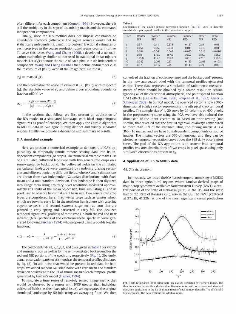
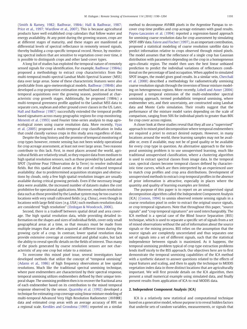
Table 1Coefficients of the double logistic regression function (Eq. (8)) used to describesimulated crop temporal profiles in the numerical example.

Coef WinterNIR

WinterRED

SummerNIR

SummerRED

OtherNIR

OtherRED

k 0.57 0.11 0.275 0.127 0.15 0.05c 0.054 −0.065 0.038 −0.041 0.018 −0.011d 0.034 −0.06 0.046 −0.033 0.016 −0.016p 95.0 110.0 167.0 167.0 158.0 158.0q 125.0 135.0 235.0 260.0 220.0 250.0vb 0.247 0.095 0.23 0.153 0.103 0.103ve 0.17 0.117 0.25 0.143 0.09 0.09

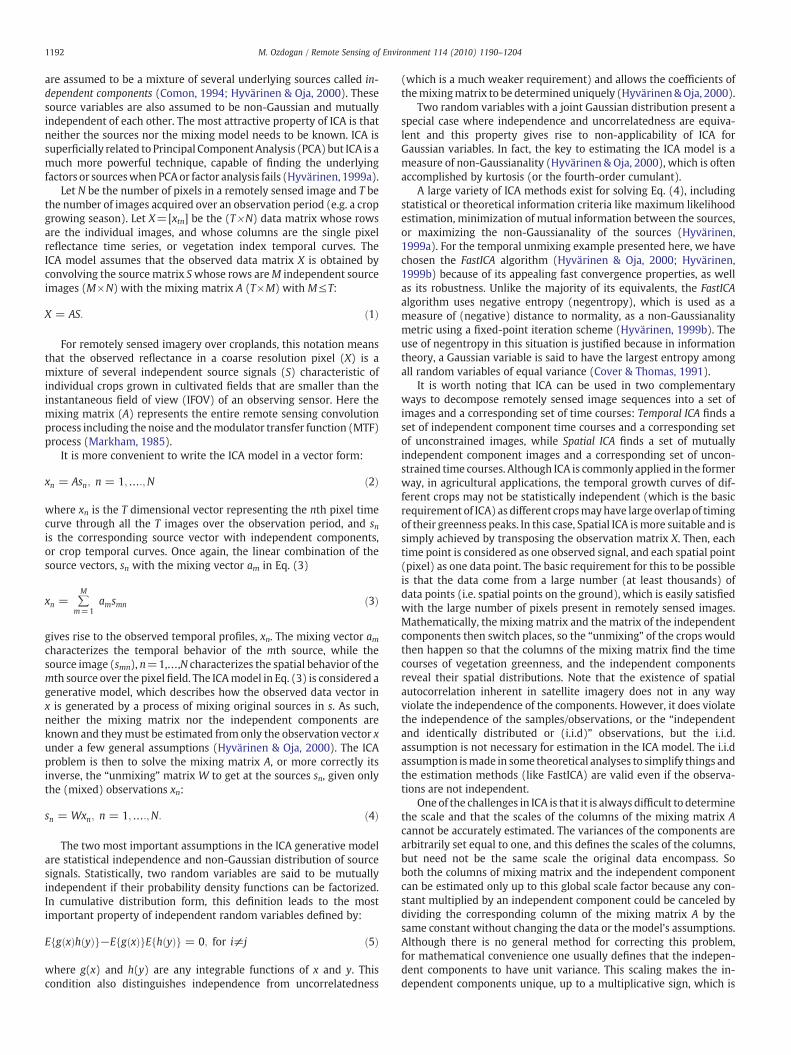
Fig. 1. NIR reflectance for all three land-use classes predicted by Fischer's model. Thethin lines show data with added random Gaussian noise with zero mean and standarddeviation equivalent to the 5% of annual mean of each temporal profile. The thick solidlines represent the data without the additive noise.


often different for each component (Comon, 1994). However, there isstill the ambiguity in the sign of the mixing matrix and the estimatedindependent components.

Finally, since the ICA method does not impose constraints onabundance fractions (otherwise the signal sources would not bestatistically independent), using it to perform fractional estimates ofeach crop type in the coarse resolution pixel seems counterintuitive.To solve this issue, Wang and Chang (2006a) developed a normali-zation methodology similar to that used in traditional linear mixturemodels. Let ICi(r) denote the value of each pixel r in ith independentcomponent. Wang and Chang (2006a) then define endmember ei asthe maximum of |ICi(r)| over all the image pixels in the ICi:

jeij = maxr jICi rð Þj ð6Þ

and then normalize the absolute value of ICi(r), |ICi(r)| with respect to|ei|, the absolute value of ei, and define a corresponding abundancefraction αICi(r) by

αICi=

jICi rð Þj−minr jICi rð Þjjeij−minrjICi rð Þj : ð7Þ

In the sections that follow, we first present an application ofthe ICA model to a simulated landscape with ideal crop temporalsignatures as proof of concept. We then apply the FastICA algorithmto MODIS data in two agriculturally distinct and widely separatedregions. Finally, we provide a discussion and summary of results.

3. A simulated example

Here we present a numerical example to demonstrate ICA's ap-plicability to temporally unmix remote sensing data into its in-dependent components (or crops). The numerical example makes useof a simulated cultivated landscape with two generalized crops on asemi-vegetative background. The cultivated fields on the simulatedagricultural landscape were generated by randomly placing rectan-gles and ellipses, depicting different fields, whose X and Y dimensionsare drawn from two independent Gaussian distributions with fixedmean and a unit standard deviation. This landscape is then digitizedinto image form using arbitrary pixel resolution measured approxi-mately at a tenth of the mean object size, thus simulating a Landsatpixel used to observe fields that are 1 ha in size. Two generalized croptypes are considered here: first, winter crops such as winter wheatwhich are sown in early fall in the northern hemisphere with a springvegetative peak; and second, summer crops such as corn that areplanted in early spring and harvested in early fall. The idealizedtemporal signatures (profiles) of these crops in both the red and nearinfrared (NIR) portions of the electromagnetic spectrum were gen-erated following Fischer (1994) who proposed using a double logisticfunction:

x tð Þ = vb +k

1 + e−c t−pð Þ −k + vb + ve1 + ed t−qð Þ : ð8Þ

The coefficients vb, ve, k, c, p, d, and q are given in Table 1 for winterand summer crops, aswell as for the semi-vegetated background for thered and NIR portions of the spectrum, respectively (Fig. 1). Obviously,actual observations are not as smooth as the temporal profiles simulatedby Eq. (8). To add noise that would be present in real data for bothcrops, we added random Gaussian noise with zero mean and standarddeviation equivalent to the 5% of annual mean of each temporal profilegenerated by Fischer's model (Fischer, 1994).

To simulate a time series of remotely sensed image matrix thatwould be observed by a sensor with IVOF greater than individualcultivated fields (i.e. themixed pixel issue), we aggregated the originalsimulated landscape by 50-fold using an averaging filter. We then

convolved the fraction of each crop type (and the background) presentin the new aggregated pixel with the temporal profiles generatedearlier. These data represent a simulation of radiometric measure-ments of what should be obtained by a coarse resolution sensor,ignoring all of the directional, atmospheric, and point spread function(PSF) effects (Lee & Kaufman, 1986; Roujean et al., 1992; Keiser &Schneider, 2008). In our ICA model, the observed vector is now a 365-dimensional (daily) vector representing the nth pixel crop temporalprofiles. The sample size N is 20 rows by 20 columns or 400 pixels.In the preprocessing stage using the PCA, we have also reduced thedimension of the input vectors to 10 based on prior testing (notshown) that revealed that the first 10 eigenvalues always contributedto more than 95% of the variance. Thus, the mixing matrix A is a365×10 matrix, and we have 10 independent components or sourceimages. The mixing vectors are 365-dimensional and they can beplotted as temporal vegetation curves over the 365 daily observationtimes. The goal of the ICA application is to recover both temporalprofiles and area distributions of two crops in pixel space using onlysimulated observations present in xn.

4. Application of ICA to MODIS data

4.1. Site descriptions

In this study,we tested the ICA-based temporal unmixing ofMODISdata in three agricultural regions where Landsat-derived maps ofmajor crop types were available: Northwestern Turkey (NWT), a cen-tral portion of the state of Nebraska (NEB) in the US, and the westhalf of the state of Kansas (KST), also in the US. The NWT (centeredat 27.31E, 41.22N) is one of the most significant cereal production


centers in Turkey and comprises roughly a million hectares domi-nated by rain-fed winter wheat (55%), sunflower (30%), and lowlandirrigated rice (4%) cultivation. Winter wheat is planted in October andNovember and harvested the following May and June. Sunflower andlowland rice are planted in late spring through early summer and areharvested in early fall. As the most important product, we concen-trated on extraction of winter wheat as the dominant winter crop andcombined sunflower and lowland rice data as the major summer cropat this location. The summer and winter crops, along with other land-cover types for the year 2003, were mapped from Landsat data withgreater than 90% class accuracy (Ozdogan, unpublished data).

The NEB site (centered at 97.65W, 40.83N) is dominated by rota-tion of corn and soybeans supported by summer irrigation. The areagrows slightly more corn than soybeans each year, along with lesseramounts of small grains and alfalfa. Corn is planted in the spring(April–May) and harvested in October and November. Soybeansare typically planted a few weeks later than corn (May–June) andharvested at the same time (October–November). For this site, weused the Cropland Data Layer (CDL) produced by the US Departmentof Agriculture (USDA) National Agricultural Statistics Service (NASS).The CDL crop-specific land-cover data layer has a ground resolution of56 m. The CDL for 2008 was produced using satellite imagery fromthe Indian Remote Sensing RESOURCESAT-1 (IRS-P6) Advanced WideField Sensor (AWiFS) collected during the 2008 growing season. Theaccuracy of the land-cover classifications in the CDL is generallybetween 85% and 95% for the producer's accuracy for the major crop-specific land-cover categories in each region (NASS, 2009).

The KST site (centered at 99.0W, 38.0N) covers the western half ofKansas in the US and consists of winter wheat, sorghum, corn, andsoybean crops as well as grasslands. Winter wheat is the dominantwinter crop, encompassing roughly 60% of grain harvested in thestate. Wheat is sown in September and October period and harvestedin early- to mid-summer. Corn and soybeans are the major summercrops in the region and together cover roughly a quarter of the totalagricultural harvest. Both crops are planted in May and June and areharvested in early- to mid-fall. For the KST site, we again utilized theNASS CDL product, but this time for three years [2006–2008]. For allthree years, the CDL crop-specific land-cover data sets were producedby applying a statistical classifier to AWiFS data collected duringthe 2006–2008 growing season at 56-meter spatial resolution (NASS,2009).

4.2. MODIS data

The MODIS instrument includes seven spectral bands that aredesigned exclusively formonitoring Earth's land surfaces (Townshend& Justice, 2002). When combined, the Terra and Aqua MODIS providesub-daily global coverage at 250- and 500-m spatial resolutions andoffer enhanced spectral, spatial, radiometric, and geometric quality forimproved mapping and monitoring of vegetation activity. To date,MODIS land data have been an integral part of the production of avariety of land-cover maps, including crop types (Friedl et al., 2002;Wardlow & Egbert, 2008; Xiao et al., 2006).

A large array of standard MODIS data products is operationallyproduced and made available to the scientific community on a timelybasis. One of these products is the Nadir Bidirectional ReflectanceDistribution Function (BRDF)-Adjusted Reflectance (NBAR) data(MOD34B4, Schaaf et al., 2002). This product provides cloud-screenedand atmospherically corrected surface reflectances for all MODIS landbands that have been corrected for viewing- and illumination-angleeffects. Currently, the NBAR data are produced at 500 m spatial reso-lution every 8 days over the calendar year, geographically organized ina MODIS tile system with the Sinusoidal Projection. In this study,we used a single calendar year of NBAR data for both the NWT site(2003) and the NEB site (2008) and three calendar years (2006–2008)

of NBAR data for the KST site, all at 8-day acquisition frequency, a totalof 46 observations per year.

For each study site, MODIS images were re-projected to theUniversal Transverse Mercator reference system and sub-scenes wereextracted covering 80,000 km2, 35,000 km2, and 10,000 km2 in theKST, NWT, and NEB sites, respectively. Each of these sub-imagesconsisted of 46 layers, made of cloud-free observations within an8-day window throughout each calendar year. There were a totalof seven multi-layer images, one for each MODIS spectral banddesigned for land observations (Townshend & Justice, 2002). Theinput to our ICA model consisted of only the red or NIR reflectanceor their combinations in the form of vegetation indices such as theSimple Ratio (SR) (Jordan, 1969) and Normalized Difference VegetationIndex (NDVI) (Rouse et al., 1973). Note that nonlinear indices suchas NDVI have not been useful in linear unmixing problems, since thesum of endmembers (however defined) does not equal the observedindex value. However, given the nonlinear nature of the ICA approach,we tested the utility of NDVI, along with the SR and red and NIRreflectances to recover the fractional cover of different crop types ineach location.

5. Results

5.1. Simulation data

By presenting 365 available images depicting daily (simulated)observations of our synthetic landscape to the FastICA algorithm,we obtained the mixing matrix of A with two columns and twoindependent source images. Analyzing these two columns of A, or themixing vectors, as well as the corresponding two source images, wefind vectors whose profiles mimic modeled temporal vegetationprofiles characteristic of winter and summer crops. What is shown inFig. 2 is temporally sampled (every 16th observation) time profiles ofwinter crops (left panel) and summer crops (right panel) in red (toprow), in NIR (second row), in SR (third row), and in NDVI (bottomrow). In all profiles, the reflectance values are standardized to unitvariance. In each of the mixing vectors, the vegetation peak (or troughin the case of red reflectance) on the temporal axis occurs at adifferent time for each crop. The location of the peak reflectance in NIRand in vegetation indices corresponds to the early season (around day140) for winter crops, and later in the season (around day 210) forsummer crops. One might question whether these temporal profilescould in fact be characteristic of temporal profiles of the cropsconsidered here. Fig. 2 also shows the observed (by Fischer's model)temporal profiles for summer and winter crops in all four spectralregions. There is a close correspondence between the “observed”and modeled temporal profiles in all spectral regions, including thevegetation indices. In some cases there is not a strong overlap ofthe two profiles, for example in NIR and SR winter profiles. This isdue to the inherent difficulty of scaling output in the ICA approach.Nevertheless, what matters most for detecting crop signatures intemporal remote sensing is the location of peaks and troughs(Wardlow et al., 2007), which are well modeled with the ICAtechnique. The simulation experiment further reveals that the ICAmethod is somewhat insensitive to spectral inputs whether they areoriginal bands or a combination of them in vegetation index form.Statistically, the correlation between “observed” and ICA-modeledtemporal profiles is similar for all four inputs. Fig. 2 also suggests thatin all cases, identification of peak (trough) location in the wintercrops' temporal profile is more accurate than for the summer crops.Such estimation errors can have many different sources, such as lackof independence of the sources, dimension reduction by PCA, outliers,and simple random effects. One other possibility for the increasedmismatch in summer crops may be related to the ordering inidentification of the independent components. However, ordering ofindependent components is generally not an issue in ICA and the

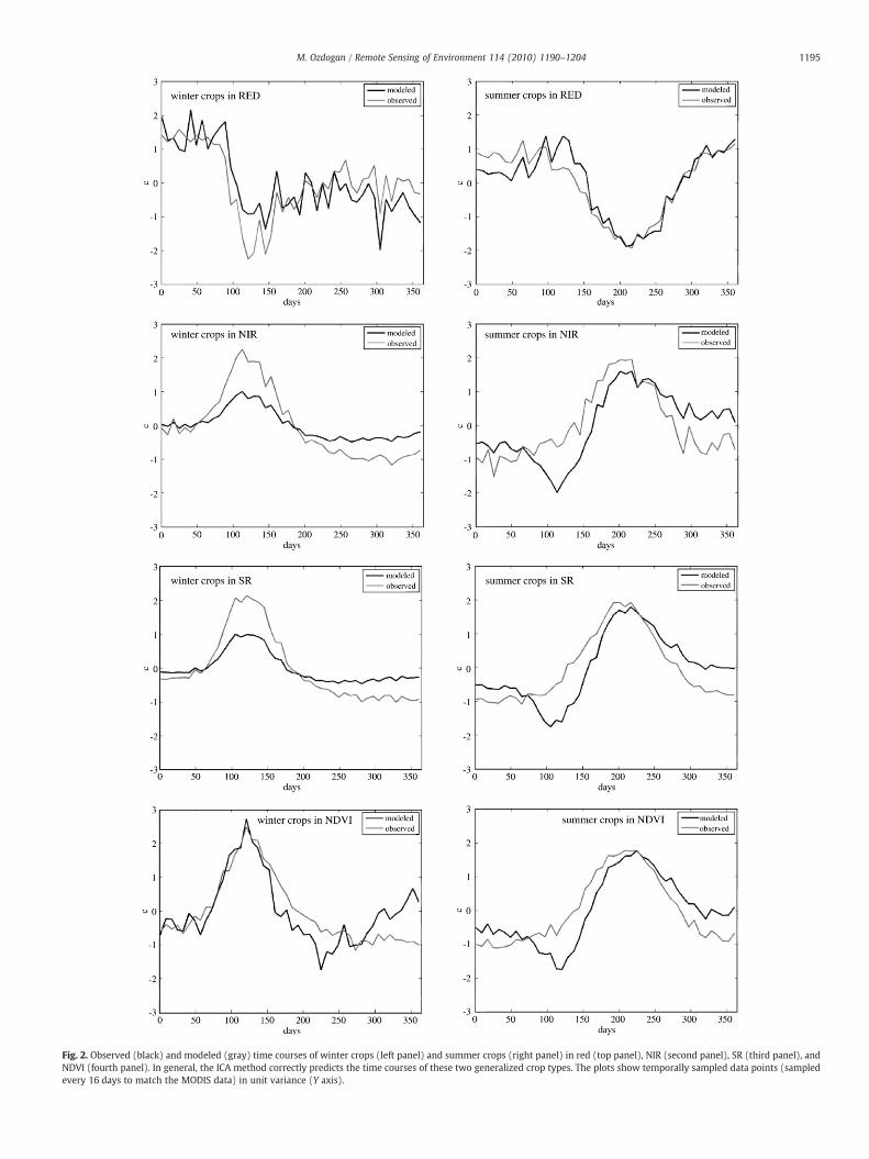
Fig. 2. Observed (black) and modeled (gray) time courses of winter crops (left panel) and summer crops (right panel) in red (top panel), NIR (second panel), SR (third panel), andNDVI (fourth panel). In general, the ICA method correctly predicts the time courses of these two generalized crop types. The plots show temporally sampled data points (sampledevery 16 days to match the MODIS data) in unit variance (Y axis).



FastICA algorithm tends to provide them in the same order. On theother hand, the order is more related to the issue of non-Gaussianality(most non-Gaussian independent component tend to come first),although this ordering too often occurs at random. To test whetherthis ordering is the source of the mismatch, we computed the normsof the columns of themixingmatrix to obtain the relative contributionof each component to the variance (not shown) and found that it wasnot the case.

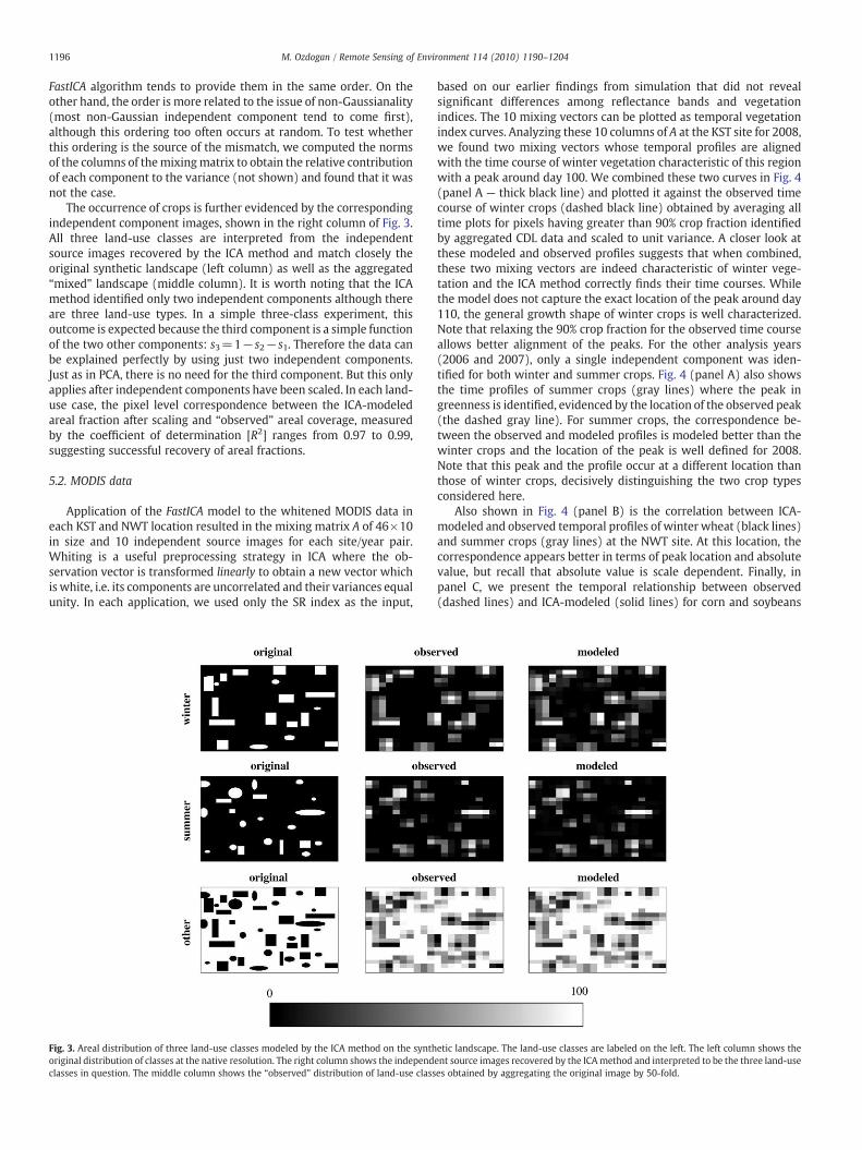
The occurrence of crops is further evidenced by the correspondingindependent component images, shown in the right column of Fig. 3.All three land-use classes are interpreted from the independentsource images recovered by the ICA method and match closely theoriginal synthetic landscape (left column) as well as the aggregated“mixed” landscape (middle column). It is worth noting that the ICAmethod identified only two independent components although thereare three land-use types. In a simple three-class experiment, thisoutcome is expected because the third component is a simple functionof the two other components: s3=1− s2−s1. Therefore the data canbe explained perfectly by using just two independent components.Just as in PCA, there is no need for the third component. But this onlyapplies after independent components have been scaled. In each land-use case, the pixel level correspondence between the ICA-modeledareal fraction after scaling and “observed” areal coverage, measuredby the coefficient of determination [R2] ranges from 0.97 to 0.99,suggesting successful recovery of areal fractions.

5.2. MODIS data

Application of the FastICA model to the whitened MODIS data ineach KST and NWT location resulted in the mixing matrix A of 46×10in size and 10 independent source images for each site/year pair.Whiting is a useful preprocessing strategy in ICA where the ob-servation vector is transformed linearly to obtain a new vector whichis white, i.e. its components are uncorrelated and their variances equalunity. In each application, we used only the SR index as the input,

Fig. 3. Areal distribution of three land-use classes modeled by the ICA method on the synthoriginal distribution of classes at the native resolution. The right column shows the independclasses in question. The middle column shows the “observed” distribution of land-use class

based on our earlier findings from simulation that did not revealsignificant differences among reflectance bands and vegetationindices. The 10 mixing vectors can be plotted as temporal vegetationindex curves. Analyzing these 10 columns of A at the KST site for 2008,we found two mixing vectors whose temporal profiles are alignedwith the time course of winter vegetation characteristic of this regionwith a peak around day 100. We combined these two curves in Fig. 4(panel A — thick black line) and plotted it against the observed timecourse of winter crops (dashed black line) obtained by averaging alltime plots for pixels having greater than 90% crop fraction identifiedby aggregated CDL data and scaled to unit variance. A closer look atthese modeled and observed profiles suggests that when combined,these two mixing vectors are indeed characteristic of winter vege-tation and the ICA method correctly finds their time courses. Whilethe model does not capture the exact location of the peak around day110, the general growth shape of winter crops is well characterized.Note that relaxing the 90% crop fraction for the observed time courseallows better alignment of the peaks. For the other analysis years(2006 and 2007), only a single independent component was iden-tified for both winter and summer crops. Fig. 4 (panel A) also showsthe time profiles of summer crops (gray lines) where the peak ingreenness is identified, evidenced by the location of the observed peak(the dashed gray line). For summer crops, the correspondence be-tween the observed and modeled profiles is modeled better than thewinter crops and the location of the peak is well defined for 2008.Note that this peak and the profile occur at a different location thanthose of winter crops, decisively distinguishing the two crop typesconsidered here.

Also shown in Fig. 4 (panel B) is the correlation between ICA-modeled and observed temporal profiles of winter wheat (black lines)and summer crops (gray lines) at the NWT site. At this location, thecorrespondence appears better in terms of peak location and absolutevalue, but recall that absolute value is scale dependent. Finally, inpanel C, we present the temporal relationship between observed(dashed lines) and ICA-modeled (solid lines) for corn and soybeans

etic landscape. The land-use classes are labeled on the left. The left column shows theent source images recovered by the ICAmethod and interpreted to be the three land-usees obtained by aggregating the original image by 50-fold.

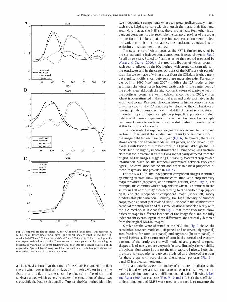
Fig. 4. Temporal profiles predicted by the ICA method (solid lines) and observed byMODIS data (dashed lines) for all sites using the SR index as input. A) KST site 2008results; B) NWT site 2003 results; and C) NEB site 2008 results. Refer to the legend forcrop types analyzed at each site. The observations were generated by averaging theresponse of MODIS SR for pixels having greater than 90% crop area in question in theaggregated “ground truth” map available for each site. Both ICA predictions andobservations are scaled to have unit variance.


at the NEB site. Note that the range of the X-axis is changed to reflectthe growing season limited to days 75 through 280. An interestingfeature of this figure is the close phenological profile of corn andsoybean crops, which generally makes the separation of these twocrops difficult. Despite this small difference, the ICA method identifies

two independent components whose temporal profiles closely matcheach crop, helping to correctly distinguish them and their fractionalarea. Note that at the NEB site, there are at least four other inde-pendent components that resemble the temporal profiles of the cropsin question. It is likely that these independent components reflectthe variation in both crops across the landscape associated withagricultural management practices.

The occurrence of winter crops at the KST is further revealed bythe corresponding independent component images, shown in Fig. 5for all three years. Scaled to fractions using the method proposed byWang and Chang (2006a), the area distribution of winter crops ineach year predicted by the ICA method with strong concentrations inthe southwest and in the center portions of the KST site (left panels)is similar to the maps of winter crops from the CDL data (right panel),but significant differences between these maps also exist. For exam-ple, both in 2006 (top) and 2007 (middle), the ICA model under-estimates the winter crop fraction, particularly in the center part ofthe study area, although the high concentrations of winter wheat inthe southeast corner are well modeled. In contrast, in 2008, winterwheat is overestimated in the central area and underestimated in thesouthwest corner. One possible explanation for higher concentrationsof winter crops in the ICA map may be related to the combination oftwo independent components with slightly different representationof winter crops to depict a single crop type. It is possible to selectonly one of these components to reflect winter crops but a singlecomponent tends to underestimate the distribution of winter cropsat this location (not shown).

The independent component images that correspond to themixingvectors further reveal the location and intensity of summer crops inthe image field for each analysis year (Fig. 6). In general, there is astrong correlation between modeled (left panels) and observed (rightpanels) distribution of summer crops in all years, although the ICAmodel tends to slightly underestimate the summer crop area fraction.Note that these fractional distributions are not easily detected from theoriginal MODIS images, suggesting ICA's ability to extract crop relatedinformation based on the temporal differences between two croptypes. The correlation coefficient and other statistical properties ofthese images are also provided in Table 2.

For the NWT site, the independent component images identifiedby mixing vectors show significant correlation with crop intensitymaps for winter (top panel) and summer (bottom) crops (Fig. 7). Forexample, the common winter crop, winter wheat, is dominant in thesouthern half of the study area according to the Landsat map (upperright) and the independent component image (upper left) nicelypredicts this phenomenon. Similarly, the high intensity of summercrops, made up mostly of lowland rice, is evident in the southwesterncorner of the study area and this same location is modeled nicely withthe ICA method. It is clear from Fig. 7 that these two maps showdifferent crops in different locations of the image field and are fullyindependent events. Again, these differences are not easily detectedfrom the original MODIS images.

Similar results were obtained at the NEB site. Fig. 8 shows thecorrelation between modeled (left panel) and observed (right panel)area fractions for corn (top panel) and soybeans (bottom panel) incentral Nebraska. The abundance of corn in the central and westernportions of the study area is well modeled and general temporalshapes of land-use types are very satisfactory. Similarly, the variabilityof soybean abundance in the northeast is captured nicely. Note thatthe close correspondence between modeled and observed fractionsfor these crops with very similar phenological patterns (Fig. 4 —

panel C) is a pleasant outcome.To quantitatively assess the quality of crop area predictions, the

MODIS-based winter and summer crop maps at each site were com-pared to existing crop maps at different spatial scales following Lobelland Asner (2004) at each site (Figs. 9, 10 and 11). Both the coefficientof determination and RMSE were used as the metric to measure the

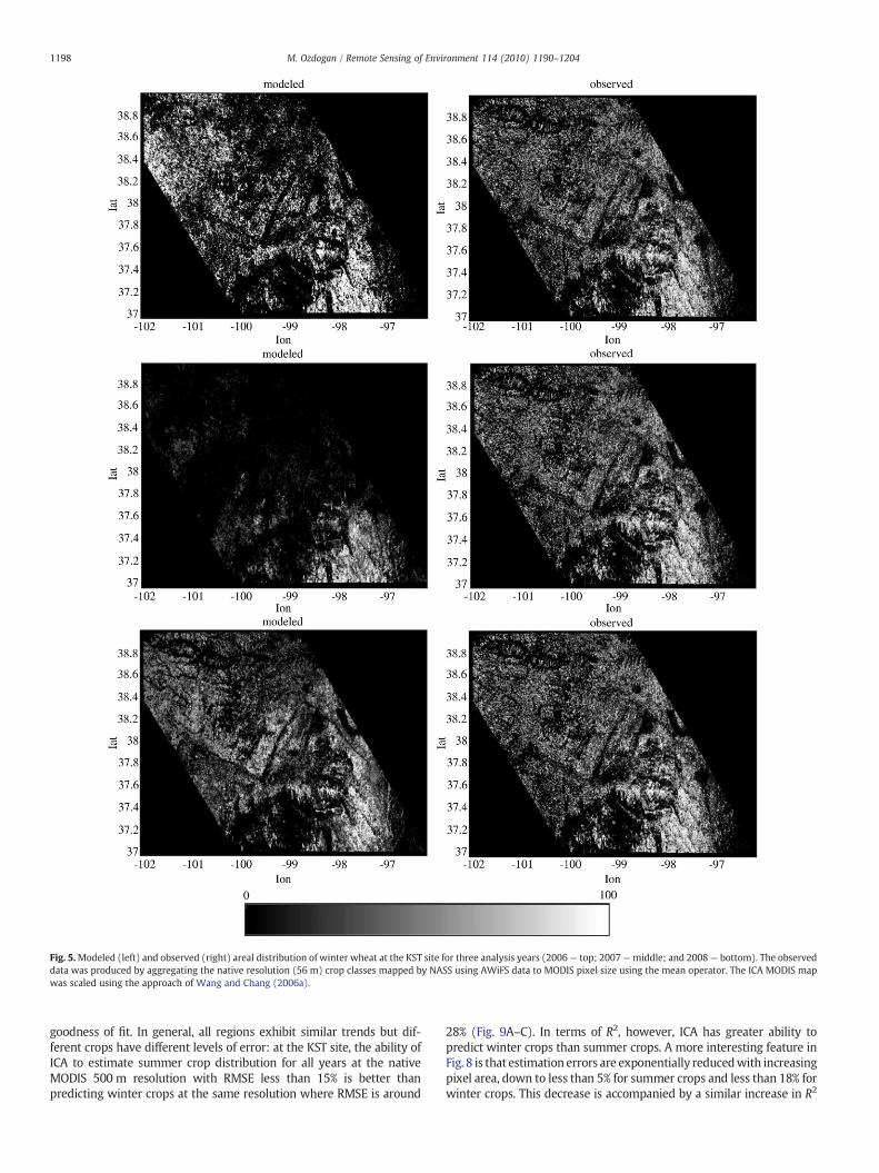
Fig. 5.Modeled (left) and observed (right) areal distribution of winter wheat at the KST site for three analysis years (2006— top; 2007—middle; and 2008— bottom). The observeddata was produced by aggregating the native resolution (56 m) crop classes mapped by NASS using AWiFS data to MODIS pixel size using the mean operator. The ICA MODIS mapwas scaled using the approach of Wang and Chang (2006a).


goodness of fit. In general, all regions exhibit similar trends but dif-ferent crops have different levels of error: at the KST site, the ability ofICA to estimate summer crop distribution for all years at the nativeMODIS 500 m resolution with RMSE less than 15% is better thanpredicting winter crops at the same resolution where RMSE is around

28% (Fig. 9A–C). In terms of R2, however, ICA has greater ability topredict winter crops than summer crops. A more interesting feature inFig. 8 is that estimation errors are exponentially reducedwith increasingpixel area, down to less than 5% for summer crops and less than 18% forwinter crops. This decrease is accompanied by a similar increase in R2

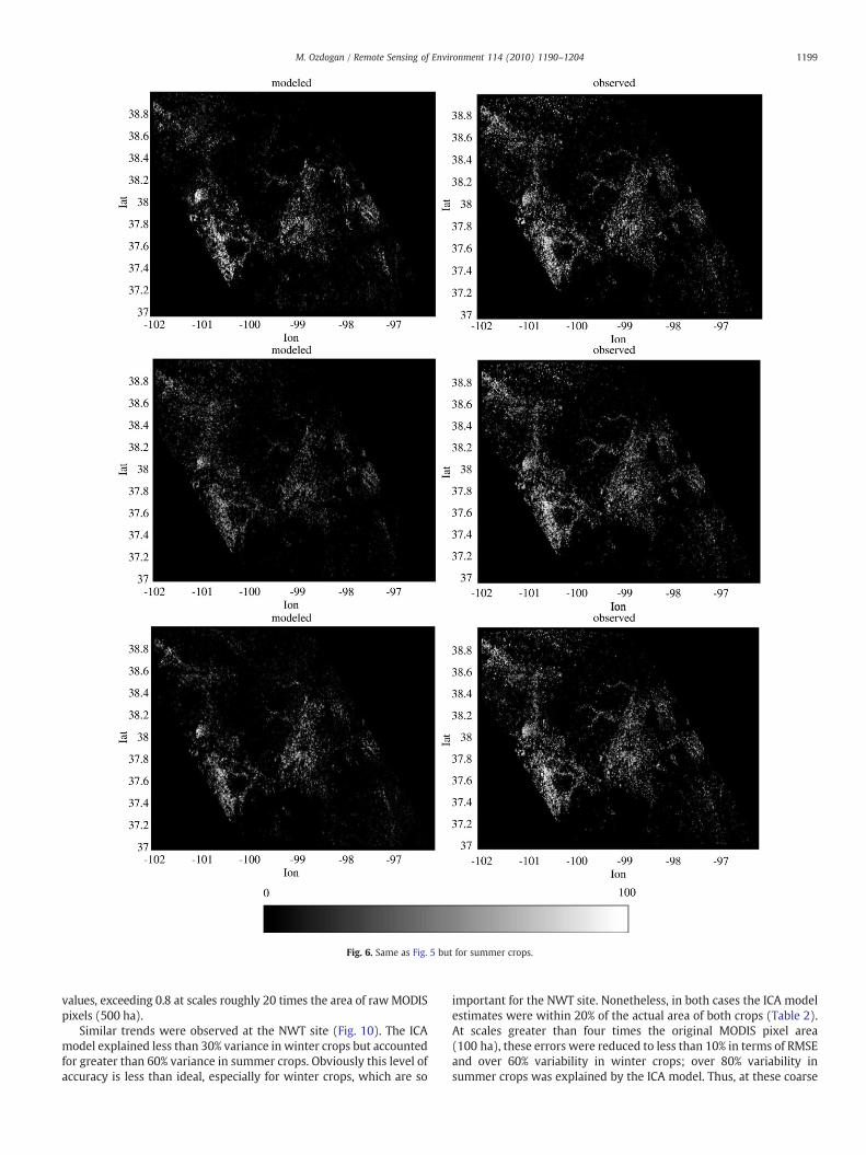
Fig. 6. Same as Fig. 5 but for summer crops.


values, exceeding 0.8 at scales roughly 20 times the area of rawMODISpixels (500 ha).

Similar trends were observed at the NWT site (Fig. 10). The ICAmodel explained less than 30% variance in winter crops but accountedfor greater than 60% variance in summer crops. Obviously this level ofaccuracy is less than ideal, especially for winter crops, which are so

important for the NWT site. Nonetheless, in both cases the ICA modelestimates were within 20% of the actual area of both crops (Table 2).At scales greater than four times the original MODIS pixel area(100 ha), these errors were reduced to less than 10% in terms of RMSEand over 60% variability in winter crops; over 80% variability insummer crops was explained by the ICA model. Thus, at these coarse

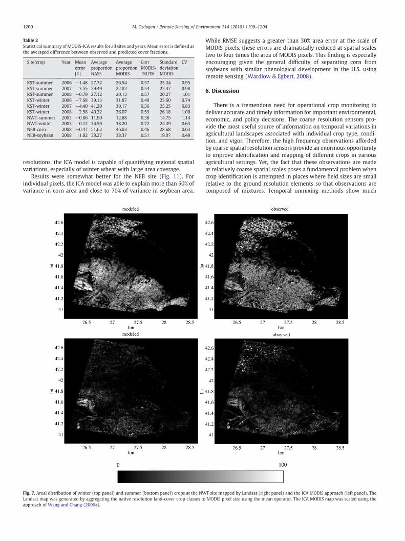
Table 2Statistical summary of MODIS-ICA results for all sites and years. Mean error is defined asthe averaged difference between observed and predicted cover fractions.

Site/crop Year Meanerror[%]

AverageproportionNASS

AverageproportionMODIS

CorrMODIS-TRUTH

StandarddeviationMODIS

CV

KST-summer 2006 −1.48 27.72 26.54 0.57 25.34 0.95KST-summer 2007 3.55 29.49 22.82 0.54 22.37 0.98KST-summer 2008 −0.79 27.12 20.13 0.57 20.27 1.01KST-winter 2006 −7.68 39.13 31.87 0.49 23.60 0.74KST-winter 2007 −4.40 41.20 30.17 0.36 25.25 0.83KST-winter 2008 −2.58 40.22 26.07 0.59 26.18 1.00NWT-summer 2003 −0.86 11.90 12.88 0.38 14.75 1.14NWT-winter 2003 0.12 34.59 38.20 0.72 24.39 0.63NEB-corn 2008 −0.47 51.62 46.03 0.46 28.68 0.63NEB-soybean 2008 11.82 38.27 38.37 0.51 19.07 0.49


resolutions, the ICA model is capable of quantifying regional spatialvariations, especially of winter wheat with large area coverage.

Results were somewhat better for the NEB site (Fig. 11). Forindividual pixels, the ICA model was able to explain more than 50% ofvariance in corn area and close to 70% of variance in soybean area.

Fig. 7. Areal distribution of winter (top panel) and summer (bottom panel) crops at the NWLandsat map was generated by aggregating the native resolution land-cover crop classes toapproach of Wang and Chang (2006a).

While RMSE suggests a greater than 30% area error at the scale ofMODIS pixels, these errors are dramatically reduced at spatial scalestwo to four times the area of MODIS pixels. This finding is especiallyencouraging given the general difficulty of separating corn fromsoybeans with similar phenological development in the U.S. usingremote sensing (Wardlow & Egbert, 2008).

6. Discussion

There is a tremendous need for operational crop monitoring todeliver accurate and timely information for important environmental,economic, and policy decisions. The coarse resolution sensors pro-vide the most useful source of information on temporal variations inagricultural landscapes associated with individual crop type, condi-tion, and vigor. Therefore, the high frequency observations affordedby coarse spatial resolution sensors provide an enormous opportunityto improve identification and mapping of different crops in variousagricultural settings. Yet, the fact that these observations are madeat relatively coarse spatial scales poses a fundamental problem whencrop identification is attempted in places where field sizes are smallrelative to the ground resolution elements so that observations arecomposed of mixtures. Temporal unmixing methods show much

T site mapped by Landsat (right panel) and the ICA MODIS approach (left panel). TheMODIS pixel size using the mean operator. The ICA MODIS map was scaled using the

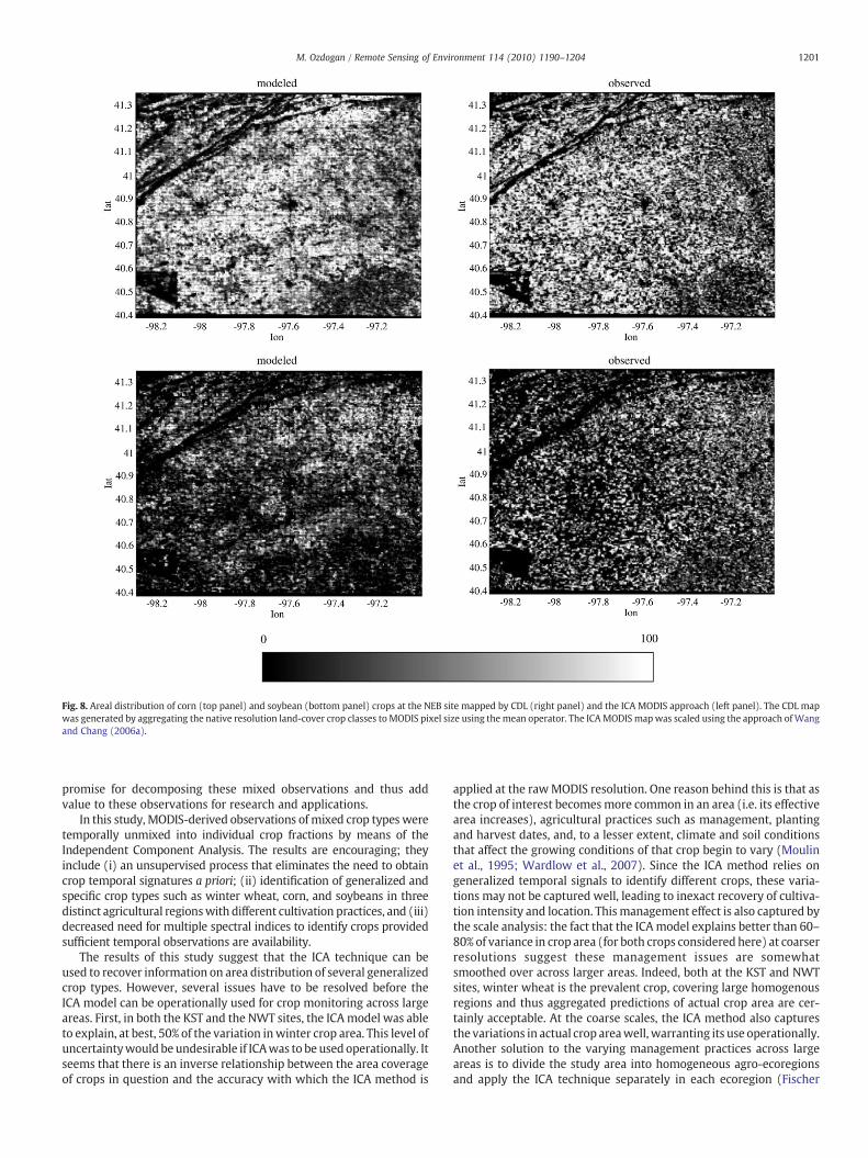
Fig. 8. Areal distribution of corn (top panel) and soybean (bottom panel) crops at the NEB site mapped by CDL (right panel) and the ICA MODIS approach (left panel). The CDL mapwas generated by aggregating the native resolution land-cover crop classes to MODIS pixel size using the mean operator. The ICAMODISmapwas scaled using the approach ofWangand Chang (2006a).


promise for decomposing these mixed observations and thus addvalue to these observations for research and applications.

In this study, MODIS-derived observations of mixed crop types weretemporally unmixed into individual crop fractions by means of theIndependent Component Analysis. The results are encouraging; theyinclude (i) an unsupervised process that eliminates the need to obtaincrop temporal signatures a priori; (ii) identification of generalized andspecific crop types such as winter wheat, corn, and soybeans in threedistinct agricultural regionswith different cultivation practices, and (iii)decreased need for multiple spectral indices to identify crops providedsufficient temporal observations are availability.

The results of this study suggest that the ICA technique can beused to recover information on area distribution of several generalizedcrop types. However, several issues have to be resolved before theICA model can be operationally used for crop monitoring across largeareas. First, in both the KST and the NWT sites, the ICAmodel was ableto explain, at best, 50% of the variation inwinter crop area. This level ofuncertaintywould be undesirable if ICAwas to be used operationally. Itseems that there is an inverse relationship between the area coverageof crops in question and the accuracy with which the ICA method is

applied at the rawMODIS resolution. One reason behind this is that asthe crop of interest becomesmore common in an area (i.e. its effectivearea increases), agricultural practices such as management, plantingand harvest dates, and, to a lesser extent, climate and soil conditionsthat affect the growing conditions of that crop begin to vary (Moulinet al., 1995; Wardlow et al., 2007). Since the ICA method relies ongeneralized temporal signals to identify different crops, these varia-tions may not be captured well, leading to inexact recovery of cultiva-tion intensity and location. Thismanagement effect is also captured bythe scale analysis: the fact that the ICAmodel explains better than 60–80% of variance in crop area (for both crops considered here) at coarserresolutions suggest these management issues are somewhatsmoothed over across larger areas. Indeed, both at the KST and NWTsites, winter wheat is the prevalent crop, covering large homogenousregions and thus aggregated predictions of actual crop area are cer-tainly acceptable. At the coarse scales, the ICA method also capturesthe variations in actual crop areawell, warranting its use operationally.Another solution to the varying management practices across largeareas is to divide the study area into homogeneous agro-ecoregionsand apply the ICA technique separately in each ecoregion (Fischer

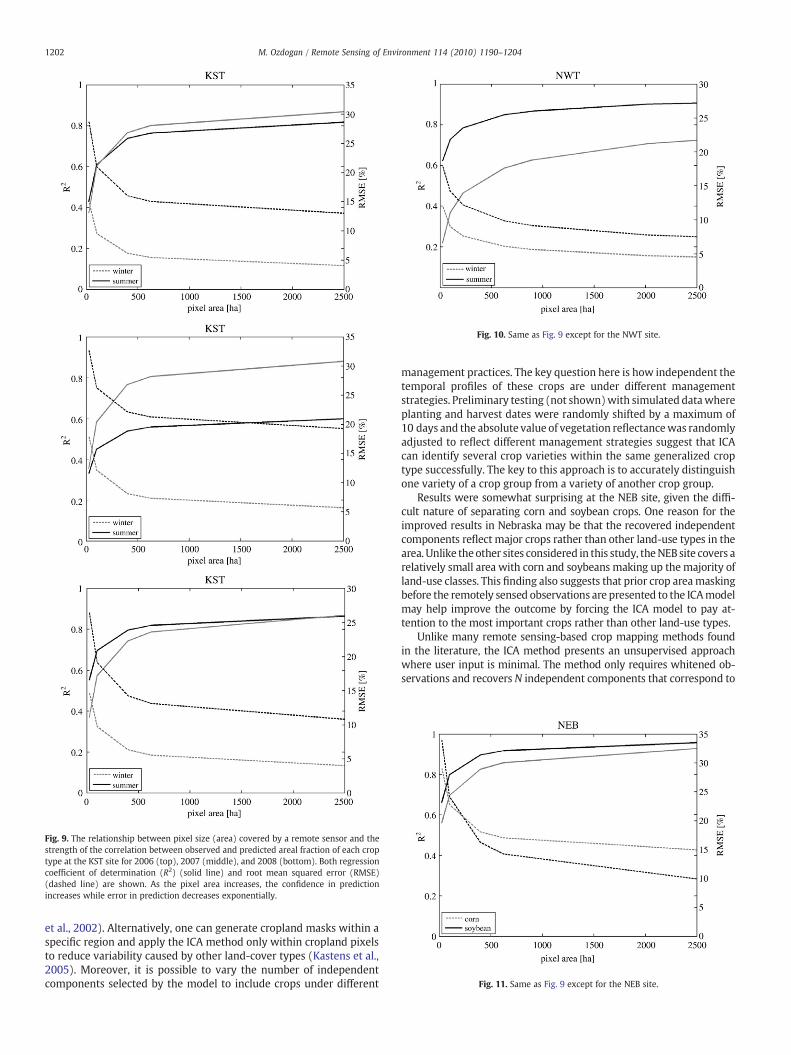
Fig. 9. The relationship between pixel size (area) covered by a remote sensor and thestrength of the correlation between observed and predicted areal fraction of each croptype at the KST site for 2006 (top), 2007 (middle), and 2008 (bottom). Both regressioncoefficient of determination (R2) (solid line) and root mean squared error (RMSE)(dashed line) are shown. As the pixel area increases, the confidence in predictionincreases while error in prediction decreases exponentially.

Fig. 10. Same as Fig. 9 except for the NWT site.

Fig. 11. Same as Fig. 9 except for the NEB site.


et al., 2002). Alternatively, one can generate cropland masks within aspecific region and apply the ICA method only within cropland pixelsto reduce variability caused by other land-cover types (Kastens et al.,2005). Moreover, it is possible to vary the number of independentcomponents selected by the model to include crops under different

management practices. The key question here is how independent thetemporal profiles of these crops are under different managementstrategies. Preliminary testing (not shown)with simulated datawhereplanting and harvest dates were randomly shifted by a maximum of10 days and the absolute value of vegetation reflectancewas randomlyadjusted to reflect different management strategies suggest that ICAcan identify several crop varieties within the same generalized croptype successfully. The key to this approach is to accurately distinguishone variety of a crop group from a variety of another crop group.

Results were somewhat surprising at the NEB site, given the diffi-cult nature of separating corn and soybean crops. One reason for theimproved results in Nebraska may be that the recovered independentcomponents reflect major crops rather than other land-use types in thearea. Unlike theother sites considered in this study, theNEB site covers arelatively small area with corn and soybeans making up themajority ofland-use classes. This finding also suggests that prior crop areamaskingbefore the remotely sensed observations are presented to the ICAmodelmay help improve the outcome by forcing the ICA model to pay at-tention to the most important crops rather than other land-use types.

Unlike many remote sensing-based crop mapping methods foundin the literature, the ICA method presents an unsupervised approachwhere user input is minimal. The method only requires whitened ob-servations and recovers N independent components that correspond to


a variety of features in the input image set, including those featurescharacteristic of different crop types (as well as those that are not). Theprimary input from the user comes at the end of the mapping process,that is, the identification of these independent components. As withPCA, the components do not always reveal physically meaningfulcharacteristics of the landscape and are often difficult to interpret. Oneway to improve the interpretation process would be to use simulatedtemporal crop growth curves obtained from various crop growthmodels and eliminate independent components that are not physicallyrepresentative of crops. Furthermore, it is possible to use the ICAmethodas a data-mining tool to pre-process the raw remotely sensed imagesinto a few physically meaningful independent components and thensubject these new sets of images to a classification process using knowntraining samples (Wang & Chang, 2006b).

The issue of the interpretability of independent components pri-marily stems from the inherent unconstrained nature of the signalsthat allows them to adopt physically improbable forms so that thecorresponding components are statistically independent (Stone et al.,2000). Put another way, ICA exploits the extra degrees of freedomimplicit in the unconstrained signals to find statistically independentsource signals in a dataset and thus, the independence of extractedsignals is achieved at the cost of physically improbable forms for theirunconstrained spatial or temporal signals. This allows the ICA to findindependent signals but not necessarily the underlying constrainedsources (Stone et al., 2000). There are, however, recent preliminarydevelopments in medical applications of ICA that successfully extractindependent components in constrained form (e.g. Van Hulle, 2008).Moreover, users often know a great deal about agricultural practicesin a region, which have been determined by many years of traditionand climate and soil resources. It has been recently shown that this apriori information can be successfully incorporated into the ICAmodelduring the signal decomposition phase so it automatically allowsextraction of only significant components (e.g. Balsi et al., 2005).

Finally, successful application of the ICA method to reflectancedata and simple vegetation indices in both the simulated and actualremote sensing observations suggests that the ICA technique can beused to extract crop related information from sensors withoutextensive sets of spectral bands, as long as the temporal availabilityof signals is available. One implication of these results concernspossible tradeoffs between temporal and spectral resolution whenselecting data from existing sensors. The results here indicate that theability to resolve crop types is dependent on temporal capabilities ofthe sensor more than the availability of spectral bands (including thenumber, location and width of these bands). The majority of spaceborne sensors today have at least one visible and one NIR spectralregion and this makes them particularly suitable for the ICA method.As a result, it may be possible to provide similar quality crop areaestimates from finer temporal resolution sensors with fewer spectralbands (AVHRR, AWiFS, or SPOT VEGETATION) when compared tosensors with somewhat improved spectral sensing capabilities (suchas Landsat ETM+ or Hyperion). Given the significant cost savingsassociated with limited spectral coverage in a sensor, the resultspresented here imply that temporally available observations may infact be a reasonable substitute for spectral coverage for crop areaestimation problems, at least withmethods involving the ICAmethod.

7. Conclusions

The use of satellite remote sensing for crop area estimation isconditioned by the frequency of the measurements, and sensors withfrequent observation capabilities provide information at moderate tocoarse spatial resolutions that results in mixed pixels. We havepresented a new unsupervised temporal unmixing methodology builton the Independent Component Analysis of satellite signals to recoverboth the time profile and area distribution of different crop types.ICA is a relatively new statistical and computational technique whose

purpose is to reveal factors hidden beneath sets of measurements.These are assumed to be amixture of several underlying sources that intheir turn are assumed to be non-Gaussian andmutually independent.The most attractive property of ICA is that neither these sources northe mixing model needs to be known. This study demonstrates thatwhen applied to time-series MODIS data in locations considered here,the ICA method is a viable tool for regional-scale and automatedmapping of generalized crop typeswith relatively good accuracies. Thegeneral, landscape-level cropping patterns for winter and summercrops depicted in the ICAmaps are similar to thosemade fromLandsat-style observations in both locations, especially when aggregated toscales greater than the native MODIS resolution (250–500 m). Theapplication of ICA for operational crop monitoring will require in-creasingly sophisticated algorithms that will take into account priorinformation on crop growth curves, constrained estimation of in-dependent components, and scaling of mixing vectors to obtainphysically possible ranges. Nevertheless, the success of the initialattempts to automatically map crop distributions across large areasusing MODIS data is particularly encouraging, given the existing andplanned observations over agriculturally important regions aroundthe world such as those from the MEdium Resolution Imaging Spec-trometer (MERIS), Advanced Wide Field Sensor (AWiFS), and Visible/Infrared Imager/Radiometer Suite (VIIRS) on board TheNational Polar-orbiting Operational Environmental Satellite System (NPOESS). Thisstudy should be viewed as an initial step in the development of anoperationalMODIS-based cropmonitoring tool based on newmachinelearning algorithms such as the ICA. At the very least ICA can be used asa data-mining tool to pre-process MODIS data into a few physicallymeaningful independent components that are then subjected to aclassification algorithm. These ICA derived components are certainly asignificant addition to other derivative products such as vegetationphenology and spectral metrics that have been found to be importantfor crop mapping across large regions.

Acknowledgements

This researchwas partly funded by the NASA Applications ProgramGrantNNX08AM69G, awarded toMutluOzdogan. The early commentsof Dr. Tobias Kuemmerle and Dr. Peter Wolter greatly improved thismanuscript. Dr. Ozdogan is also indebted to Mr. George Allez for hismeticulous editing that improved the readability of this document.Finally, the author is indebted to Dr. Aapo Hyvärinen of the Universityof Helsinki for making the FastICA tool publicly available and for adiscussion in its use for remote sensing data analysis.

References

Adams, J. B., Smith, M. O., & Johnson, P. E. (1986). Spectral mixture modeling: A newanalysis of rock and soil types at Viking Lander I site. Journal of Geophysical Research,91, 8098−8112.

Allen, J. D. (1990). A look at the remote sensing applications program of the NationalAgricultural Statistics Service. Journal of Official Statistics, 6, 393−409.

Badhwar, G. D. (1984). Automatic corn–soybean classification using LandsatMSS data. I.Near-harvest crop proportion estimation. Remote Sensing of Environment, 14(1–3),15−29.

Badhwar, G. D. (1984). Automatic corn–soybean classification using Landsat MSS data.II. Early season crop proportion estimation. Remote Sensing of Environment, 14(1–3),31−37.

Badhwar, G. D. (1984). Classification of corn and soybeans using multitemporalthematic mapper data. Remote Sensing of Environment, 16(2), 175−181.

Balsi, M., Filosa, G., Valente, G., & Pantano, P. (2005). Constrained ICA for functionalmagnetic resonance imaging. Proceedings of the 2005 European Conference on circuittheory and design, 28 August–2 September, 2005, Vol. 2, II/67–II/70.

Carfagna, E., & Javier Gallego, F. (2005). Using remote sensing for agricultural statistics.International Statistical Review, 73(3), 389−404.

Cherchali, S., Amram, O., & Flouzat, G. (2000). Retrieval of temporal profiles of reflectancesfrom simulated and real NOAA-AVHRR data over heterogeneous landscapes. Inter-national Journal of Remote Sensing, 21(4), 753−775.

Comon, P. (1994). Independent Component Analysis: A new concept? Signal Processing,36(3), 287−314.

Cover, T. M., & Thomas, J. A. (1991). Elements of information theory.NewYork: JohnWiley& Sons 542 pp.


Deaton, A., & Laroque, G. (1992). On the behavior of commodity prices.Review of EconomicStudies, 59(1), 1−23.

Faivre, R., & Fischer, A. (1997). Predicting crop reflectances using satellite data observingmixed pixels. Journal of Agricultural, Biological, and Environmental Statistics, 2(1),87−107.

Famine Early Warning System (FEWS) (2005). Famine early warning system networkhome page, USAID FEWS NET.

Fischer, A. (1994). A simple model for the temporal variations of NDVI at regional scaleover agricultural countries. Validation with ground radiometric measurements.International Journal of Remote Sensing, 15(7), 1421−1446.

Fischer, G., van Velthuizen, H., Shah,M., & Nachtergaele, F. (2002). Global agro-ecologicalassessment for agriculture in the 21st century: Methodology and results (researchreport RR-02-02). Laxenburg, Austria: International Institute for Applied SystemsAnalysis (IIASA) and Food and Agriculture Organization (FAO) of the UnitedNations(UN).

Friedl, M. A., McIver, D. K., Hodges, J. C. F., Zhang, X. Y., Muchoney, D., Strahler, A. H.,et al. (2002). Global land cover mapping fromMODIS: Algorithms and early results.Remote Sensing of Environment, 83, 287−302.

Hall, Forrest G., & Badhwar, Gautam D. (1987). Signature-extendable technology:Global space-based crop recognition. IEEE Transactions on Geoscience and RemoteSensing, GE-25(1), 93−103.

Hanuschak, G., Hale, R., Craig, M., Mueller, R., & Hart, G. (2001). The new economics ofremote sensing for agricultural statistics in the United States. Proc. of the Conferenceon agricultural and environmental statistical applications in Rome (CAESAR), Vol. 2.(pp. XXII.1−XXII.10) June 5–7.

Hyvärinen, A. (1999). Survey on independent component analysis. Neural ComputingSurveys, 2, 94−128.

Hyvärinen, A. (1999). Fast and robust fixed-point algorithms for Independent ComponentAnalysis. IEEE Transactions on Neural Networks, 10(3), 626−634.

Hyvärinen, A., & Oja, E. (2000). Independent component analysis, algorithms andapplications. Neural Networks, 13(4–5), 411−430.

Jordan, C. F. (1969). Derivation of leaf area index from quality measurements of light onthe forest floor. Ecology, 50, 663−666.

Kastens, J. J., Kastens, T. L., Kastens, D. L. A., Price, K. P., Martinko, E. A., & Lee, R. Y. (2005).Image masking for crop yield forecasting using AVHRR NDVI time series imagery.Remote Sensing of Environment, 99, 341−356.

Keiser, G., & Schneider, W. (2008). Estimation of sensor point spread function by spatialsubpixel analysis. International Journal of Remote Sensing, 29(7), 2137−2155.

Kerdiles, H., & Grondona, M. (1995). NOAA-AVHRR NDVI decomposition and subpixelclassification using linear mixing in the Argentina Pampa. International Journal ofRemote Sensing, 16, 1303−1325.

Lee, T. Y., & Kaufman, Y. J. (1986). Non-Lambertian effects on remote sensing of surfacereflectance and vegetation index. IEEE Transactions on Geoscience and Remote Sensing,24, 699−708.

Lobell, D. B., & Asner, G. P. (2004). Cropland distributions from temporal unmixing ofMODIS data. Remote Sensing of Environment, 93, 412−422.

Markham, B. L. (1985). The Landsat sensors' spatial responses. IEEE Transactions onGeoscience and Remote Sensing, GE-23(6), 864−875.

Menenti, M., Azzali, S., Verhoef, W., & Van Swol, R. (1993). Mapping agro-ecologicalzones and time lag in vegetation growth by means of Fourier analysis of time seriesof NDVI images. Advances in Space Research, 13, 233−237.

Moulin, S. A., Fischer, G. Dedieu, & Delecolle, R. (1995). Temporal variations in satellitereflectances at field and regional scales compared with values simulated by linkingcrop growth and SAIL models. Remote Sensing of Environment, 54(3), 261−272.

NASS (2009). National Agricultural Statistics Service (NASS), Cropland Data Layer (2008)NASS Cropland Data Layer webpage http://www.nass.usda.gov/research/Cropland/SARS1a.htm (last accessed 27 November 2009).

Nelson, G. C. (2002). Introduction to the special issue on spatial analysis for agriculturaleconomists. Agricultural Economics, 27, 197−200.

Ozdogan, M., & Woodcock, C. E. (2006). Resolution dependent errors in remote sensingof cultivated areas. Remote Sensing of Environment, 103, 203−217.

Price, K. P., Egbert, S. L., Nellis, M. D., Lee, R. Y., & Boyce, R. (1997). Mapping land cover ina high plains agro-ecosystem using a multidate Landsat thematic mapper modelingapproach. Transactions of the Kansas Academy of Science, 100(1–2), 21−33.

Puyou-Lascassies, P., Flouzat, G., Gay, M., & Vignolles, C. (1994). Validation of the use ofmultiple linear regression as a tool for unmixing coarse spatial resolution images.Remote Sensing of Environment, 49, 155−166.

Quarmby, N. A., Townshend, J. R. G., Settle, J. J., White, K. H., Milnes, M., Hindle, T. L., &Silleos, N. (1992). Linear mixture modeling applied to AVHRR data for crop areaestimation. International Journal of Remote Sensing, 13(3), 415−425.

Roujean, J. -L., Leroy, M., & Deschamps, P. Y. (1992). A bidirectional reflectance model ofthe Earth's surface for the correction of remote sensing data. Journal of GeophysicalResearch, 97, 20,455−20,468.

Rouse, J. W., Haas, R. H., Schell, J. A., & Deering, D. W. (1973). Monitoring vegetationsystems in the great plains with ERTS. Third ERTS symposium, NASA SP-351, vol. I.(pp. 309−317).

Schaaf, C. B., Gao, F., Strahler, A. H., Lucht, W., Li, X., Tsang, T., et al. (2002). Firstoperational BRDF, Albedo and Nadir reflectance products from MODIS. RemoteSensing of Environment, 83, 135−148.

Smith, J. H., & Ramey, D. B. (1982). A crop area estimator based on changes in thetemporal profile of a vegetative index. American Statistical Association: Proceed-ings of the Survey Research Methods Section 495–498.

Stone, J. V., Porril, J., Porter, N. R., & Hunkin, N. M. (2000). Spatiotemporal ICA of fMRIdata. Computational neuroscience report, vol. 202. (pp. 7).

Townshend, J. R. G., & Justice, C. (2002). Towards operational monitoring of terrestrialsystems by moderate-resolution remote sensing. Remote Sensing of Environment,83, 351−359.

Van Hulle, M. M. (2008). Constrained subspace ICA based on mutual informationoptimization directly. Neural Computation, 20(4), 964−973.

Vyas, S. P., Oza, M. P., & Dadhwal, V. K. (2005). Multi-crop separability study of Rabicrops using multi-temporal satellite data. Journal of Indian Society of RemoteSensing, 33(1), 75−79.

Wang, J., & Chang, C. -I. (2006). Applications of Independent Component Analysis (ICA)in endmember extraction and abundance quantification for hyperspectral imagery.IEEE Transactions on Geoscience and Remote Sensing, 44(9), 2601−2616.

Wang, J., & Chang, C. -I. (2006). Independent component analysis-based dimensionalityreduction with applications in hyperspectral image analysis. IEEE Transactions onGeoscience and Remote Sensing, 44(6), 1586−1600.

Wardlow, B. D., & Egbert, S. L. (2008). Large-area crop mapping using time-seriesMODIS 250 m NDVI data: An assessment for the U.S. Central Great Plains. RemoteSensing of Environment, 112, 1096−1116.

Wardlow, B. D., Egbert, S. L., & Kastens, J. H. (2007). Analysis of time-series MODIS 250m vegetation index data for crop classification in the U.S. Central Great Plains.Remote Sensing of Environment, 108(3), 290−310.

Xiao, X., Boles, S., Frolking, S., Li, C., Babu, J. Y., Salas, W., et al. (2006). Mapping paddyrice agriculture in South and Southeast Asia using multi-temporal MODIS images.Remote Sensing of Environment, 100, 95−113.

You, L., Wood, S., Wood-Sichra, U., & Chamberlin, J. (2004). Generating plausible cropdistribution maps for sub-Sahara Africa using spatial allocation model. InformationDevelopment, 23(2–3), 151−159.

http://www.nass.usda.gov/research/Cropland/SARS1a.htm

http://www.nass.usda.gov/research/Cropland/SARS1a.htm

Documents

Remote Sensing of Environment - USGS & Javier Gallego, 2005; Hanuschak et al., 2001; Wardlow & Egbert, 2008). ... data and Monte Carlo simulation. Their results suggest that the