Remote Water Quality Monitoring Network

Data Report of Baseline Conditions for 2010 — 2013Susquehanna River Basin Commission

Publication No. 297 June 2015

Executive Summary

Dawn R. Hintz, Environmental Scientist/Database Analyst

Luanne Y. Steffy, Aquatic Ecologist

Contact: Dawn HintzPhone: (717) 238-0423 Email: dhintz@srbc.net

In 2010, the Susquehanna River Basin Commission (SRBC) initiated a real-time, continuous water quality monitoring network (RWQMN) to monitor the water quality in small, headwater streams that would potentially be impacted by unconventional natural gas drilling. The monitoring network is currently comprised of 59 stations. In addition to monitoring pH, temperature, dissolved oxygen, specific conductance, and turbidity continuously, metals, nutrients, ions, and radionuclides are sampled on a quarterly basis at each monitoring station. Macroinvertebrates, commonly used as indicators of the biological health and integrity of streams, are collected at each station annually. These data continue to build a baseline dataset for smaller streams in the basin.

The monitoring stations are located within three Level III ecoregions: North Central Appalachian (NCA), Northern Appalachian Plateau and Uplands (NAPU), and Central Appalachian Ridges and Valleys (Ridges and Valleys). The majority of the stations are located in the NCA and NAPU

ecoregions. In order to determine if natural gas drilling is having an impact on the monitored watersheds, the monitoring stations were grouped by ecoregion and analyses were ran on the water chemistry and biological data.

The NCA ecoregion is a largely forested region that is distinctly different from the NAPU and Ridges and Valleys ecoregions in both water chemistry and biological data. Median specific conductance and turbidity concentrations are significantly different from the other two ecoregions. Specific conductance and turbidity were not significantly different between the monitored years. The lowest median values for both parameters are found in the NCA ecoregion.

The NAPU and Ridges and Valleys ecoregions are more closely related. Specific conductance and turbidity values by ecoregion are significantly different from the other ecoregion. However, when looking at median turbidity and specific conductance concentrations by year within the

NAPU ecoregion, some years are more closely related to a year within the Ridges and Valleys ecoregion and vice versa. Macroinvertebrate IBI scores do not show a significant difference between the ecoregions.

Well pad density was compared to summer water temperatures and macroinvertebrate IBI scores. There was no correlation found between water temperature or IBI score and well pad density. Macroinvertebrate IBI score was also compared to drilled well density and well distance from the monitoring station; again, no correlation was seen. The best correlation to macroinvertebrate IBI score was instream habitat score. The valuable datasets collected within the RWQMN have proven to be not only useful in analyzing the data for potential gas drilling impacts, but also impacts from construction, agriculture, development, climate change and other activities influencing the water quality parameters and biological communities.

Photo: West Creek, Cameron County, Pa.

SRBC • 4423 N. Front St. • Harrisburg, PA 17110 • 717-238-0423 • 717-238-2436 Fax • www.srbc.net

2

Parameters and EquipmentEach RWQMN station contains the following equipment: data sonde, data platform, and a power source – typically a solar panel. The data sonde is a multi-parameter water quality sonde with optical dissolved oxygen and turbidity probes, a pH probe, and a conductance and temperature probe. The data sonde also includes a non-vented relative depth sensor. The entire unit is placed in protective housing and secured in free-flowing water at each site. Water chemistry data are recorded every five minutes and transmitted to an in-house database every two to four hours.

The data are uploaded to a public web site maintained by SRBC. The web site allows users to view, download, graph, and determine basic statistics from the raw data. General project information and maps are also found on the user-friendly web site at http://mdw.srbc.net/remotewaterquality/.

IntroductionIn 2010, the Susquehanna River Basin Commission (SRBC) established a real-time, continuous water quality monitoring network called the Remote Water Quality Monitoring Network (RWQMN). The initial purpose of the project was to monitor small headwater streams for potential impacts from natural gas drilling as 85 percent of the Susquehanna River Basin is underlain with natural gas shales. Since 2008, unconventional gas drilling by means of hydraulic fracturing (fracking) has greatly increased throughout the basin. However, the applicability of a continuous, real-time data network is not limited to the impacts of gas drilling. The RWQMN allows SRBC and other agencies/groups to gain a better understanding of water quality conditions in headwater streams and monitor impacts from any activities in the watershed.

The RWQMN currently includes 59 continuous monitoring stations; 58 of the stations have been monitoring pH, specific conductance (conductance), temperature, dissolved oxygen (DO), and turbidity for a minimum period of one year (Appendix B). The data for these 58 stations, through December 31, 2013, are included in the analysis covered in this report (Appendix A).

In order to supplement the continuous monitoring data, additional water chemistry parameters are collected quarterly. These additional parameters include metals, nutrients, common cations/anions, and radionuclides. Macroinvertebrate samples are collected in October at every station and fish are sampled at select stations during the spring/summer season. Beginning in 2014, fish will be sampled annually on a rotating basis at each site. The continuous and supplemental sampling data collected at each station have resulted in a substantial baseline dataset for smaller streams in Pennsylvania and New York, where previously very little data existed.

Data sonde at Pleasant Creek, Lycoming County, Pa. The data sonde is a multi-parameter water quality sonde with optical dissolved oxygen and turbidity probes, a pH probe, and a conductance and temperature probe. The data sonde also includes a non-vented relative depth sensor. The entire unit is placed in protective housing and secured in free-flowing water at each site.

Data platform.

Data sonde.

3

Map 1. RWQMN Stations Shown with Level III Ecoregions

Monitoring Station BackgroundThe majority of the Susquehanna River Basin is underlain with natural gas shales (85 percent); these natural gas shales are mainly located in two Level III ecoregions – North Central Appalachian and Northern Appalachian Plateau and Uplands (Wood and others, 1996). Within the RWQMN, 31 monitoring stations are located in the North Central Appalachian ecoregion and 22 monitoring stations are located in the Northern Appalachian Plateau and Uplands ecoregion (Map 1). The remaining six monitoring stations are located in the Central Appalachian Ridges and Valleys ecoregion. Table 1 contains a station list and descriptive characteristics for each of the watersheds. Elk Run, Tioga County, Pa.

4

Table 1. RWQMN Station List with Basic Watershed Characteristics

Watershed Name Dominant Landuse(s) Watershed Size (mi2)

Bedrock Geology

Impaired Miles1

% Impaired Stream Miles1

SRBC Well Pad Approvals*2

PADEP Horizontal Well Drilling Permits

Issued*2

Northern Appalachian Plateau and Uplands

Apalachin Creek Forest (70%)Agriculture (26%) 43 Shale 0 0% 11 20

Baldwin Creek Forest (73%)Agriculture (21%) 35 Shale 0 0% 0 0

Canacadea Creek Forest (70%)Agriculture (23%) 47 Shale 0 0% 0 0

Cherry Valley Creek Forest (67%)Agriculture (23%) 51 Shale 0 0% 0 0

Choconut Creek Forest (73%)Agriculture (23%) 38 Shale 0 0% 10 8

East Branch Wyalusing Creek Forest (51%)Agriculture (45%) 69 Sandstone 4.3 3% 40 154

Hammond Creek Agriculture (51%)Forest (46%) 29 Shale 0 0% 12 22

Little Mehoopany Creek Forest (68%)Agriculture (26%) 11 Sandstone 0 0% 8 24

Meshoppen Creek Forest (48%)Agriculture (48%) 52 Sandstone 0 0% 66 153

Nanticoke Creek Forest (62%)Agriculture (34%) 48 Shale 0 0% 0 0

Sangerfield River Forest (35%)Agriculture (32%) 52 Shale 0 0% 0 0

Sing Sing Creek Forest (60%)Agriculture (21%) 35 Shale 0 0% 0 0

Snake Creek Forest (68%)Agriculture (28%) 45 Sandstone 0 0% 21 57

South Branch Tunkhannock Creek Forest (55%)Agriculture (32%) 70 Sandstone 26.7 22% 0 0

Sugar Creek Agriculture (51%)Forest (48%) 56 Sandstone 10.8 13% 46 209

Sugar Run Forest (65%)Agriculture (31%) 33 Sandstone 0 0% 23 48

Tomjack Creek Agriculture (55%)Forest (42%) 27 Shale 0 0% 21 25

Trout Brook Forest (64%)Agriculture (31%) 36 Shale 0 0% 0 0

Upper Catatonk Creek Forest (70%)Agriculture (16%) 30 Shale 0 0% 0 0

Upper Crooked Creek Agriculture (53%)Forest (44%) 47 Shale 0 0% 19 32

Upper Tuscarora Creek Agriculture (52%)Forest (42%) 53 Shale 0 0% 0 0

Wappasening Creek Forest (64%)Agriculture (33%) 47 Shale 1.8 2% 23 30

North Central AppalachianBaker Run Forest (99%) 35 Sandstone 0 0% 9 16

Blockhouse Creek Forest (75%)Agriculture (21%) 38 Sandstone 0 0% 10 32

Bowman Creek Forest (90%) 54 Sandstone 0.3 1% 0 0

Driftwood Branch Forest (93%)Grassland (5%) 83 Sandstone 0 0% 6 35

East Branch Fishing Creek Forest (93%) 13 Sandstone 23.7 100% 0 0*As tracked by SRBC1 PA 2014 Integrated List and NY State 2012 Priority Waterbodies List2 Multiple wells can be located on one pad. Data last updated January 2015.

5

Watershed Name Dominant Landuse(s) Watershed Size (mi2)

Bedrock Geology

Impaired Miles

% Impaired Stream Miles1

SRBC Well Pad Approvals*2

PADEP Horizontal Well Drilling Permits

Issued*2

East Fork Sinnemahoning Creek Forest (89%)Grassland (10%) 33 Sandstone 0 0% 2 4

Elk Run Forest (82%)Agriculture (11%) 21 Sandstone 0 0% 20 25

Grays Run Forest (95%) 16 Sandstone 5.1 15% 9 16

Hicks Run Forest (92%) 34 Sandstone 0 0% 3 5

Hunts Run Forest (91%) 31 Sandstone 0 0% 0 0

Kettle Creek Forest (84%)Agriculture (10%) 81 Sandstone 0 0% 6 6

Kitchen Creek Forest (88%) 20 Sandstone 1.8 5% 0 1

Lackawanna River Forest (68%)Agriculture (23%) 38 Sandstone 4.3 6% 0 0

Larrys Creek Forest (76%)Agriculture (22%) 29 Sandstone 1.8 4% 24 63

Little Pine Creek Forest (83%)Agriculture (13%) 180 Sandstone 7.1 2% 41 148

Long Run Forest (81%)Agriculture (14%) 21 Sandstone 0 0% 0 0

Loyalsock Creek Forest (86%)Grassland (9%) 27 Sandstone 0 0% 0 0

Marsh Creek (Tioga County) Forest (71%)Agriculture (22%) 78 Sandstone 14.8 12% 32 38

Moose Creek Forest (95%) 3 Sandstone 0 0% 1 1

Ninemile Run Forest (85%) 16 Sandstone 0 0% 6 2

Pine Creek Forest (80%)Agriculture (11%) 385 Sandstone 23.8 3% 81 101

Pleasant Stream Forest (89%)Grassland (9%) 21 Sandstone 0 0% 0 0

Portage Creek Forest (92%)Grassland (4%) 71 Sandstone 0 0% 1 2

Starrucca Creek Forest (74%)Agriculture (18%) 52 Sandstone 0 0% 1 0

Tioga River Forest (88%)Grassland (9%) 14 Sandstone 4.2 18% 5 25

Trout Run Forest (91%)Grassland (8%) 33 Sandstone 1.5 3% 9 40

Upper Pine Creek Forest (75%)Agriculture (17%) 19 Sandstone 0 0% 0 0

West Branch Pine Creek Forest (86%)Grassland (13%) 70 Sandstone 0 0% 1 1

West Creek Forest (84%)Agriculture (7%) 59 Sandstone 3.8 3% 2

3

Young Womans Creek Forest (97%) 41 Sandstone 0 0% 0 0

Ridges and ValleysBobs Creek Forest (92%) 17 Sandstone 0 0% 0 3

Chest Creek Forest (60%)Agriculture (35%) 44 Shale 30.8 25% 0 0

Little Clearfield Creek Forest (74%)Agriculture (22%) 44 Sandstone 0 0% 0 7

Little Muncy Creek Forest (57%)Agriculture (39%) 51 Sandstone 1.8 2% 23 77

Marsh Creek Forest (88%)Agriculture (11%) 44 Sandstone 17.1 20% 1 0

West Branch Susquehanna River Forest (73%)Agriculture (20%) 36 Shale 37.0 63% 0 0

6

North Central Appalachian (NCA) EcoregionThe North Central Appalachian ecoregion is a forested, sedimentary upland that has high hills and low mountains. It encompasses the majority of the West Branch Susquehanna River Subbasin and spans across Lycoming, Sullivan, Luzerne, Wyoming, and Lackawanna Counties (Map 1). The land use is dominated by forest, with 65 percent of the region being forested in the Susquehanna River Basin (Map 2). Over 2000 square miles of the NCA ecoregion is covered with state forest providing a large arena for outdoor recreational activities (SRBC, 2013). Forestry and recreational activities are the major contributors to the economy in the ecoregion (Sayler, 2014). It is divided into two subecoregions, a glaciated eastern region and unglaciated western region. The monitoring stations are located throughout both subecoregions.

With forests dominating the landscape in the NCA ecoregion, the majority of the RWQMN stations are located in heavily forested watersheds. Forests

comprise over 90 percent of the land use in 10 of the monitored watersheds and only five monitored watersheds have less than 80 percent forested land use.

There are a variety of designated uses assigned to the monitored streams in the NCA ecoregion. The designated uses include exceptional value (EV), high-quality cold water fisheries (HQ-CWF), high quality trout stocked fisheries (HQ-TSF), cold water fisheries (CWF), trout stocked fisheries (TSF), and warm water fisheries (WWF). Exceptional value waters comprise 16 percent of the nearly 3000 stream miles monitored. Approximately 3.5 percent of the monitored stream miles are listed as not meeting the designated uses with acid deposition being the most common source of impairment. Eighteen stations meet their designated uses. The entire watershed of East Branch Fishing Creek is listed as impaired by acid deposition and Grays Run, Kitchen Creek, Tioga River, and Bowman Creek each have small sections impaired by acid deposition. The Lackawanna River

has several miles listed as impaired by natural sources and Pine Creek and Marsh Creek (Tioga County) are listed as impaired by urban sources. Little Pine Creek, Trout Run, West Creek, and Larrys Creek are short segments listed as impaired by abandoned mine drainage (AMD).

Continuous data from the RWQMN in the NCA ecoregion generally indicate good water chemistry. The mean DO concentrations range from 10.3 to 11.8 mg/l with 20 stations having a mean DO concentration of over 11 mg/l. Overall, the water temperatures remain cool in these streams with mean temperatures ranging from 8.4°C to 12.1°C. The large forested tracts provide canopy cover and erosion control which helps to maintain cooler water temperatures, which in turn sustains higher DO concentrations.

Water clarity, or turbidity, can also influence stream temperature and DO levels (USEPA, 2015). Turbidity is a measurement of water clarity–how much the material suspended in water will decrease the passage of light through the water. Material suspended in the water will absorb more heat, increasing the water temperature and lowering the DO levels because warmer water holds less DO. Median turbidity values range from 0.0 to 7.23 Nephelometric Turbidity Units (NTU) in the NCA ecoregion. Marsh Creek and Pine Creek are the only stations with median turbidity values greater than 5.0 NTU; the average turbidity in the ecoregion is 1.03 NTU. Marsh Creek is a slow, meandering stream that is impacted by agriculture and urban influences and Pine Creek is a large stream system (385 mi2) and in general, larger systems tend to have higher turbidity.

The range of median pH values show slightly acidic to neutral systems (5.9 – 7.5). The low concentrations of alkalinity and calcium, shown in the lab chemistry analyses, indicate these Staff samples fish along Marsh Creek, Tioga County, Pa., in the North Central

Appalachian Ecoregion.

7

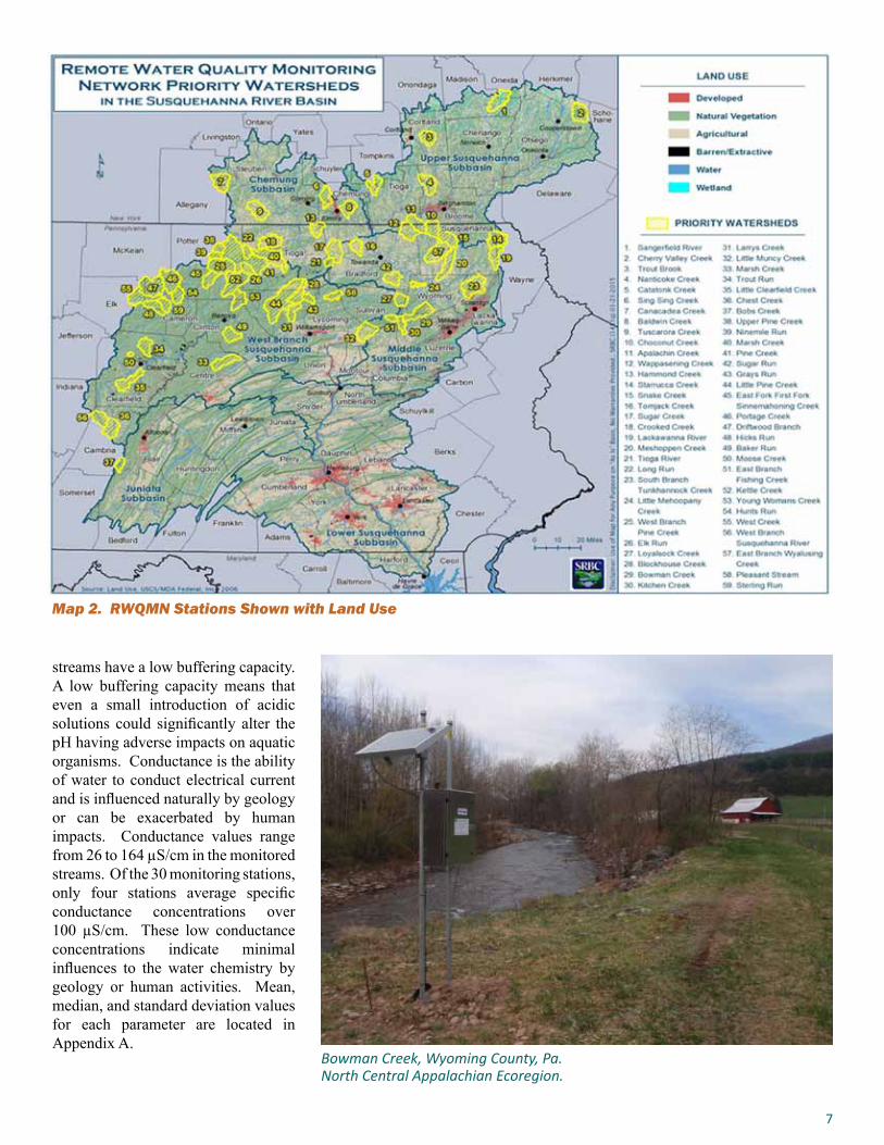
Map 2. RWQMN Stations Shown with Land Use

streams have a low buffering capacity. A low buffering capacity means that even a small introduction of acidic solutions could significantly alter the pH having adverse impacts on aquatic organisms. Conductance is the ability of water to conduct electrical current and is influenced naturally by geology or can be exacerbated by human impacts. Conductance values range from 26 to 164 µS/cm in the monitored streams. Of the 30 monitoring stations, only four stations average specific conductance concentrations over 100 µS/cm. These low conductance concentrations indicate minimal influences to the water chemistry by geology or human activities. Mean, median, and standard deviation values for each parameter are located in Appendix A.

Bowman Creek, Wyoming County, Pa.North Central Appalachian Ecoregion.

8

contributing watersheds. In the NAPU ecoregion, only five watersheds are greater than 70 percent forested while the NCA ecoregion only has one watershed that is less than 70 percent forested. Agricultural land uses comprise over 50 percent of the area in five watersheds in the NAPU ecoregion; agricultural land uses in the NCA ecoregion were greater than 20 percent at only four RWQMN stations (maximum 23 percent).

Two subecoregions make up the NAPU ecoregion – the Glaciated Low Plateau and Northeastern Uplands. The two subecoregions share similar characteristics with the Northeastern Uplands having a greater lake and bog density and steeper stream gradient (Woods and others, 1999). Six stations are located in the Northeastern Uplands subecoregion: Apalachin Creek, Meshoppen Creek, Wappasening Creek, Snake Creek, East Branch Wyalusing Creek and Choconut Creek — the remaining stations are located in the Glaciated Low Plateau subecoregion.

There is a wide range of designated uses for the 22 watersheds in the NAPU ecoregion. These uses include HQ-CWF, CWF, TSF, and WWF in Pa. and C, C(T), C(TS), B and AA in NY. Class C indicates fisheries are supported by the waterbody and it is protected for non-contact activities. Classes C(T) and C(TS) are Class C water which may support a trout population and trout spawning, respectively. Class B supports contact activities and Class AA is a drinking water source. Only four watersheds are listed as not meeting their designated uses. Sugar Creek and Wappasening Creek each have impairments from agriculture. East Branch Wyalusing Creek and South Branch Tunkhannock Creek are impaired by municipal point sources and South Branch Tunkhannock Creek is impaired by urban and unknown sources.

Northern Appalachian Plateau and Uplands (NAPU)EcoregionThe Northern Appalachian Plateau and Uplands ecoregion spans the northern portion of the Susquehanna River Basin (Map 1). It covers the majority of the New York portion of the basin and Pennsylvania counties along the NY/PA state border. This area has experienced a significant amount of the natural gas activity in recent years. Susquehanna, Bradford, and Tioga Counties, located along the PA/NY border in the NAPU ecoregion, comprise more than half

of the gas well pad approvals in the basin (SRBC, 2015). Twenty-two of the monitoring stations are located in this ecoregion.

Rolling hills and fertile valleys make this ecoregion more conducive to agricultural activities than the NCA ecoregion. However, forested land still covers over 58 percent of the area and agricultural land uses cover almost 32 percent of the ecoregion in the Susquehanna River Basin (Map 2). When comparing these monitoring stations to those in the NCA ecoregion, land use is a major difference in the

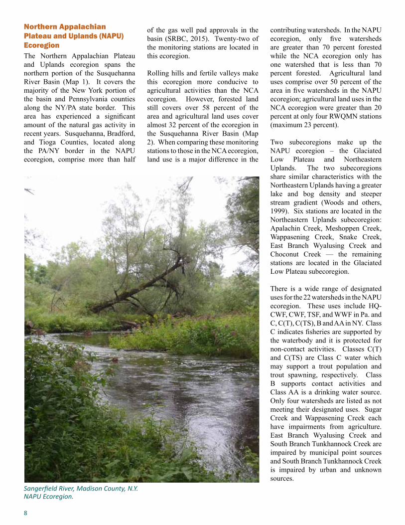
Sangerfield River, Madison County, N.Y. NAPU Ecoregion.

9

Central Appalachian Ridges and Valleys (Ridges and Valleys) EcoregionThe Central Appalachian Ridges and Valleys ecoregion is an area of parallel ridges and valleys with folded and faulted bedrock. Long, even ridges with long valleys in between dominate the landscape. Natural gas development pressure has been relatively low in this ecoregion in the Susquehanna River Basin; because of this, only six monitoring stations are located in this ecoregion.

These six monitoring stations are grouped together because they are located in the same ecoregion, but the watershed characteristics vary causing the water chemistry and biological data to differ. There are three designated uses assigned to the six monitored watersheds — HQ-CWF, CWF, and WWF. Bobs Creek and Little Clearfield Creek are the only stations meeting their designated uses. Chest Creek and West Branch Susquehanna River each are impaired by AMD. Chest Creek, Little Muncy Creek, and Marsh Creek (Centre County) have stream segments impaired by agricultural sources. Erosion from derelict land is a source of impairment for Chest Creek and the West Branch Susquehanna River; the West Branch Susquehanna River is also listed as impaired by on-site waste water and unknown sources. Overall, approximately 18 percent of the monitored stream miles in the Ridges and Valleys are not meeting their designated uses.

Conductance concentrations range from 76 – 634 µS/cm. Bobs Creek, mean concentration of 76 µS/cm, is 92 percent forested and has no impaired stream miles; the West Branch Susquehanna River, mean concentration of 634 µS/cm, is 73 percent forested and has 37 impaired stream miles (63 percent of the stream miles). The remaining four stations have specific conductance concentrations scattered throughout

Overall, the continuous data in the streams in the NAPU ecoregion exhibit good water chemistry. The mean dissolved oxygen concentrations range from 8.8 to 11.7 mg/l with only two stations having mean concentrations of less than 10 mg/l. Mean water temperatures range from 7.9°C to 16.1°C with the highest temperatures located in watersheds with the least amount of forested land use. Median pH values, range of 7.0 to 8.1, indicate neutral and basic systems.

Median turbidity values in the NAPU ecoregion range from 0.9 to 10.54 NTU; 3.3 NTU is the average turbidity observed in the ecoregion. Cherry Valley Creek and Nanticoke Creek are the only two stations to exceed 5.0 NTU; both of these monitoring stations are located in large, slow moving pools allowing for extended periods of turbidity after a storm or other turbidity-causing events.

Conductance shows the greatest range of all of the parameters (86 – 452 µS/cm) between the monitoring stations in this ecoregion. The NAPU ecoregion can be divided into two subecoregions: six monitoring stations are located in the Northeastern Uplands and the remaining stations are located in the Glaciated Low Plateau. The mean conductance range in the Northeastern Uplands is 94 – 152 µS/cm and 86 – 452 µS/cm in the Glaciated Plateau subecoregion. Glacial till geology underlays the majority of the NAPU ecoregion and can influence conductance.

the range. DO concentrations do not vary much between the monitoring locations (10.6 – 11.2 mg/l) nor do the pH values. The pH ranges from 7.2 to 7.8 indicating slightly basic systems. The water temperature ranges from 9.7°C to 14.5°C, which is most likely a result of the months used to determine the average temperature. West Branch Susquehanna River has the lowest average water temperature, but the limited dataset (14 months) contains more cool water months compared to warm water months. Little Clearfield Creek has the highest average water temperature, but is missing data from cool water months the first year it was installed.

Turbidity ranged from 2.05 to 7.2 NTU in the Ridges and Valleys ecoregion; the average turbidity in the ecoregion is 2.8 NTU. Chest Creek was the only station to have a median value greater than 5.0 NTU. This station is located downstream of Patton Borough, Cambria County, Pa., and has a gravel/sediment substrate. It is also bordered for many miles by a flood protection berm which is mowed grass. The mowed grass allows for minimal infiltration of overland flow and the substrate easily re-suspends material.

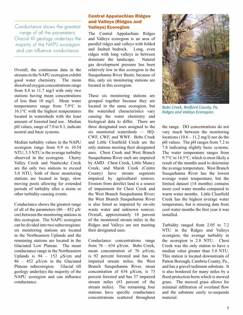
Bobs Creek, Bedford County, Pa. Ridges and Valleys Ecoregion.

Conductance shows the greatest range of all the parameters.

Glacial till geology underlays the majority of the NAPU ecoregion and can influence conductance.

10

there was no significant difference or interaction between ecoregion and year (p=0.44). The Tukey Method grouped the ecoregions using mean concentrations, significantly different means are grouped with different letters, and a box plot provides a graphical representation of the differences in conductance (Figure 1). The Tukey Method assigns letter groupings from highest to lowest mean conductance. The NAPU ecoregion has the highest mean conductance and was grouped as A, the NCA ecoregion had the lowest mean conductance and was grouped as C, and the Ridges and Valleys ecoregion fell in the middle and was grouped as B.

The NCA ecoregion shows the least variability of conductance with small quartile and outlier ranges (Figure 1). The stations in this ecoregion are mainly forested watersheds with little human impacts. The NAPU and Ridges and Valleys ecoregions show greater variability with larger quartile and outlier ranges. The NAPU ecoregion is underlain with glacial till geology, which does impact the conductance of a stream. The Ridges and Valleys ecoregion only has five monitoring stations included in the analysis and these stations vary

in land use and stream impairments; the small sample size and watershed characteristics can help explain the variability seen in the box plot.

Specific Conductance and Turbidity by Ecoregion

Natural gas drilling in the Susquehanna River Basin has brought two continuous field parameters to the forefront: conductance and turbidity. The chemicals used in natural gas fracking produce flowback with very high specific conductance concentrations. Any significant spill or leak into a waterbody will quickly influence the conductance of the stream adversely impacting water quality.

Turbidity is important because of the land disturbance activities associated with natural gas drilling. New roads, additional truck traffic on existing roads, well pad construction, and pipeline construction under and through streams can negatively impact the water quality with increased siltation, which will be seen with increased turbidity levels.

Box plots were created using the continuous records for conductance and turbidity by ecoregion. Monthly median values of conductance and turbidity were calculated for each station and then grouped by ecoregion. The box plots show the median value and quartile ranges. The lower and upper edges of the box represent the lower and upper quartiles, respectively, and the line inside the box represents the median value. Twenty-five percent of the data are less than the lower quartile and 25 percent of the data are greater than the upper quartile. The lines (whiskers) extending from the box represent the maximum and minimum values excluding outliers.

A two-way ANOVA was performed to determine if there was a significant difference (α=0.05) in conductance between ecoregions and between years within each ecoregion. There was a significant difference between ecoregions (p<0.001); however,

Figure 1. Monthly Median Conductance Concentration by Ecoregion (2010 – 2013)

Table 2 shows the grouping information for conductance means by ecoregion and year using the Tukey Method. The groupings indicate the interaction between the ecoregions and years. Within the NCA ecoregion, each of the years was more closely related to each other than any year in the NAPU or Ridges

Ecoregion Year GroupingNAPU 2012 A

NAPU 2013 A

NAPU 2011 A B

NAPU 2010 A B

Ridges & Valleys 2013 A B

Ridges & Valleys 2012 A B

Ridges & Valleys 2011 B

Ridges & Valleys 2010 B

NCA 2013 C

NCA 2010 C

NCA 2012 C

NCA 2011 C

Table 2. Ecoregion and Year Specific Conductance Grouping using Tukey Method (α=0.05)

11

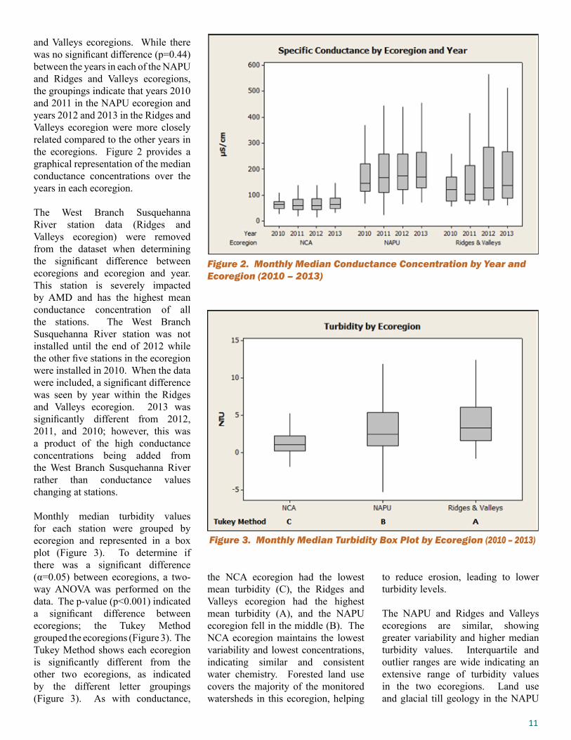
Figure 2. Monthly Median Conductance Concentration by Year and Ecoregion (2010 – 2013)

and Valleys ecoregions. While there was no significant difference (p=0.44) between the years in each of the NAPU and Ridges and Valleys ecoregions, the groupings indicate that years 2010 and 2011 in the NAPU ecoregion and years 2012 and 2013 in the Ridges and Valleys ecoregion were more closely related compared to the other years in the ecoregions. Figure 2 provides a graphical representation of the median conductance concentrations over the years in each ecoregion.

The West Branch Susquehanna River station data (Ridges and Valleys ecoregion) were removed from the dataset when determining the significant difference between ecoregions and ecoregion and year. This station is severely impacted by AMD and has the highest mean conductance concentration of all the stations. The West Branch Susquehanna River station was not installed until the end of 2012 while the other five stations in the ecoregion were installed in 2010. When the data were included, a significant difference was seen by year within the Ridges and Valleys ecoregion. 2013 was significantly different from 2012, 2011, and 2010; however, this was a product of the high conductance concentrations being added from the West Branch Susquehanna River rather than conductance values changing at stations.

Monthly median turbidity values for each station were grouped by ecoregion and represented in a box plot (Figure 3). To determine if there was a significant difference (α=0.05) between ecoregions, a two-way ANOVA was performed on the data. The p-value (p<0.001) indicated a significant difference between ecoregions; the Tukey Method grouped the ecoregions (Figure 3). The Tukey Method shows each ecoregion is significantly different from the other two ecoregions, as indicated by the different letter groupings (Figure 3). As with conductance,

the NCA ecoregion had the lowest mean turbidity (C), the Ridges and Valleys ecoregion had the highest mean turbidity (A), and the NAPU ecoregion fell in the middle (B). The NCA ecoregion maintains the lowest variability and lowest concentrations, indicating similar and consistent water chemistry. Forested land use covers the majority of the monitored watersheds in this ecoregion, helping

Figure 3. Monthly Median Turbidity Box Plot by Ecoregion (2010 – 2013)

to reduce erosion, leading to lower turbidity levels.

The NAPU and Ridges and Valleys ecoregions are similar, showing greater variability and higher median turbidity values. Interquartile and outlier ranges are wide indicating an extensive range of turbidity values in the two ecoregions. Land use and glacial till geology in the NAPU

12

Figure 4. Monthly Median Turbidity by Ecoregion and Year (2010 – 2013)

Ecoregion Year GroupingRidges & Valleys 2011 A

Ridges & Valleys 2012 A B C

NAPU 2011 A B

Ridges & Valleys 2013 A B C

NAPU 2012 A B C

Ridges & Valleys 2010 A B C D E F

NAPU 2013 C D

NAPU 2010 B C D E

NCA 2011 D E F

NCA 2012 E F

NCA 2010 D E F

NCA 2013 F

Table 3. Ecoregion and Year Turbidity Grouping using Tukey Method (α=0.05)

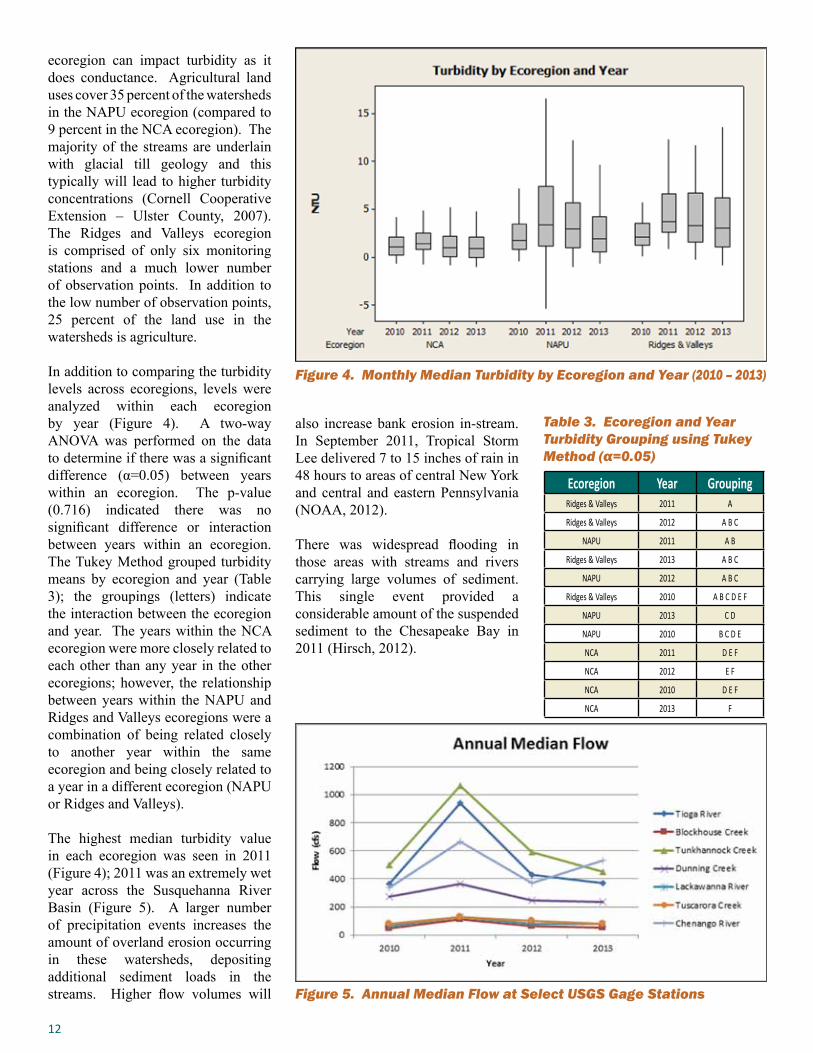
ecoregion can impact turbidity as it does conductance. Agricultural land uses cover 35 percent of the watersheds in the NAPU ecoregion (compared to 9 percent in the NCA ecoregion). The majority of the streams are underlain with glacial till geology and this typically will lead to higher turbidity concentrations (Cornell Cooperative Extension – Ulster County, 2007). The Ridges and Valleys ecoregion is comprised of only six monitoring stations and a much lower number of observation points. In addition to the low number of observation points, 25 percent of the land use in the watersheds is agriculture.

In addition to comparing the turbidity levels across ecoregions, levels were analyzed within each ecoregion by year (Figure 4). A two-way ANOVA was performed on the data to determine if there was a significant difference (α=0.05) between years within an ecoregion. The p-value (0.716) indicated there was no significant difference or interaction between years within an ecoregion. The Tukey Method grouped turbidity means by ecoregion and year (Table 3); the groupings (letters) indicate the interaction between the ecoregion and year. The years within the NCA ecoregion were more closely related to each other than any year in the other ecoregions; however, the relationship between years within the NAPU and Ridges and Valleys ecoregions were a combination of being related closely to another year within the same ecoregion and being closely related to a year in a different ecoregion (NAPU or Ridges and Valleys).

The highest median turbidity value in each ecoregion was seen in 2011 (Figure 4); 2011 was an extremely wet year across the Susquehanna River Basin (Figure 5). A larger number of precipitation events increases the amount of overland erosion occurring in these watersheds, depositing additional sediment loads in the streams. Higher flow volumes will

also increase bank erosion in-stream. In September 2011, Tropical Storm Lee delivered 7 to 15 inches of rain in 48 hours to areas of central New York and central and eastern Pennsylvania (NOAA, 2012).

There was widespread flooding in those areas with streams and rivers carrying large volumes of sediment. This single event provided a considerable amount of the suspended sediment to the Chesapeake Bay in 2011 (Hirsch, 2012).

Figure 5. Annual Median Flow at Select USGS Gage Stations

13

Continuous Stream Temperature Data

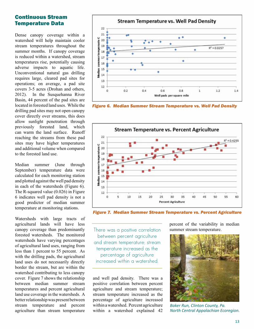
Dense canopy coverage within a watershed will help maintain cooler stream temperatures throughout the summer months. If canopy coverage is reduced within a watershed, stream temperatures rise, potentially causing adverse impacts to aquatic life. Unconventional natural gas drilling requires large, cleared pad sites for operations; on average, a pad site covers 3-5 acres (Drohan and others, 2012). In the Susquehanna River Basin, 44 percent of the pad sites are located in forested land uses. While the drilling pad sites may not open canopy cover directly over streams, this does allow sunlight penetration through previously forested land, which can warm the land surface. Runoff reaching the streams from these pad sites may have higher temperatures and additional volume when compared to the forested land use.

Median summer (June through September) temperature data were calculated for each monitoring station and plotted against the well pad density in each of the watersheds (Figure 6). The R-squared value (0.026) in Figure 6 indicates well pad density is not a good predictor of median summer temperature at monitoring stations.

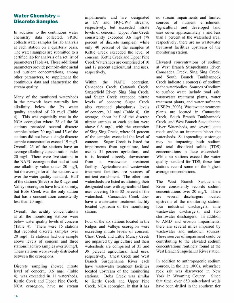
Watersheds with large tracts of agricultural lands will have less canopy coverage than predominantly forested watersheds. The monitored watersheds have varying percentages of agricultural land uses, ranging from less than 1 percent to 55 percent. As with the drilling pads, the agricultural land uses do not necessarily directly border the stream, but are within the watershed contributing to less canopy cover. Figure 7 shows the relationship between median summer stream temperatures and percent agricultural land use coverage in the watersheds. A better relationship was present between stream temperature and percent agriculture than stream temperature

and well pad density. There was a positive correlation between percent agriculture and stream temperature; stream temperature increased as the percentage of agriculture increased within a watershed. Percent agriculture within a watershed explained 42

Figure 6. Median Summer Stream Temperature vs. Well Pad Density

Figure 7. Median Summer Stream Temperature vs. Percent Agriculture

There was a positive correlation between percent agriculture

and stream temperature; stream temperature increased as the

percentage of agriculture increased within a watershed.

percent of the variability in median summer stream temperature.

Baker Run, Clinton County, Pa.North Central Appalachian Ecoregion.

14

Water Chemistry – Discrete Samples

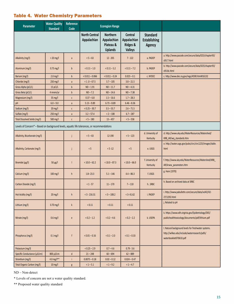
In addition to the continuous water chemistry data collected, SRBC collects water samples for lab analysis at each station on a quarterly basis. The water samples are submitted to a certified lab for analysis of a set list of parameters (Table 4). These additional parameters provide point-in-time metal and nutrient concentrations, among other parameters, to supplement the continuous data and characterize the stream quality.

Many of the monitored watersheds in the network have naturally low alkalinity, below the PA water quality standard of 20 mg/l (Table 4). This was especially true in the NCA ecoregion where 28 of the 30 stations recorded several discrete samples below 20 mg/l and 15 of the stations did not have a single discrete sample concentration exceed 19 mg/l. Overall, 23 of the stations have an average alkalinity concentration under 20 mg/l. There were five stations in the NAPU ecoregion that had at least one alkalinity value under 20 mg/l, but the average for all the stations was over the water quality standard. Half of the stations (three) in the Ridges and Valleys ecoregion have low alkalinity, but Bobs Creek was the only station that has a concentration consistently less than 20 mg/l.

Overall, the acidity concentrations at all the monitoring stations were below water quality levels of concern (Table 4). There were 15 stations that recorded discrete samples over 20 mg/l: 12 stations had one sample above levels of concern and three stations had two samples over 20 mg/l. These stations were evenly distributed between the ecoregions.

Discrete sampling showed nitrate level of concern, 0.6 mg/l (Table 4), was exceeded in 11 watersheds. Kettle Creek and Upper Pine Creek, NCA ecoregion, have no stream

impairments and are designated as EV and HQ-CWF streams, respectively, but exceeded nitrate levels of concern. Upper Pine Creek consistently exceeded 0.6 mg/l (78 percent of discrete samples), while only 40 percent of the samples at Kettle Creek exceeded the level of concern. Kettle Creek and Upper Pine Creek Watersheds are comprised of 10 and 17 percent agricultural land uses, respectively.

Within the NAPU ecoregion, Canacadea Creek, Catatonk Creek, Sangerfield River, Sing Sing Creek, and Sugar Creek exceeded nitrate levels of concern; Sugar Creek also exceeded phosphorus levels of concern, 0.1 mg/l (Table 4). On average, about half of the discrete nitrate samples at each station were above 0.6 mg/l, with the exception of Sing Sing Creek, where 91 percent of the samples exceeded the level of concern. Sugar Creek is listed for impairments from agriculture, land use is 51 percent agriculture, and it is located directly downstream from a wastewater treatment facility. Agriculture and wastewater treatment facilities are sources of nutrient enrichment. The other four watersheds are listed as attaining their designated uses with agricultural land uses covering 16 to 32 percent of the watershed. Canacadea Creek does have a wastewater treatment facility located upstream of the monitoring station.

Four of the six stations located in the Ridges and Valleys ecoregion were exceeding nitrate levels of concern. Chest Creek and Little Muncy Creek are impaired by agriculture and their watersheds are comprised of 35 and 39 percent agricultural land uses, respectively. Chest Creek and West Branch Susquehanna River each have wastewater treatment facilities located upstream of the monitoring stations. Bobs Creek was similar to Kettle Creek and Upper Pine Creek, NCA ecoregion, in that it has

no stream impairments and limited sources of nutrient enrichment. Agricultural and developed land uses cover approximately 7 and less than 1 percent of the watershed area, respectively; there are no wastewater treatment facilities upstream of the monitoring station.

Elevated concentrations of sodium at West Branch Susquehanna River, Canacadea Creek, Sing Sing Creek, and South Branch Tunkhannock Creek indicate a source(s) of sodium to the waterbodies. Sources of sodium to surface water include road salt, wastewater treatment plants, water treatment plants, and water softeners (USEPA, 2003). Wastewater treatment plants are located in Canacadea Creek, South Branch Tunkhannock Creek, and West Branch Susquehanna River Watersheds, and several state roads and/or an interstate bisect the watersheds. Salt spreading or storage may be impacting both sodium and total dissolved solids (TDS) concentrations in these watersheds. While no stations exceed the water quality standard for TDS, these four stations record some of the highest average concentrations.

The West Branch Susquehanna River consistently records sodium concentrations over 20 mg/l. There are several dischargers located upstream of the monitoring station: four industrial dischargers, nine wastewater dischargers, and two stormwater dischargers. In addition to AMD and erosion impairments, there are several miles impaired by wastewater and unknown sources. These sources of impairment could be contributing to the elevated sodium concentrations routinely found at the West Branch Susquehanna River station.

In addition to anthropogenic sodium sources, in the late 1800s, subsurface rock salt was discovered in New York in Wyoming County. Since that time, over 650 salt-related wells have been drilled in the southern tier

15

Table 4. Water Chemistry Parameters

ParameterWater Quality

StandardReference

CodeEcoregion Range

North Central Appalachian

Northern Appalachian

Plateau & Uplands

Central Appalachian

Ridges & Valleys

Standard Establishing

Agency

Alkalinity (mg/l) > 20 mg/l a < 5 – 63 12 - 205 7 - 122 a. PADEPa. http://www.pacode.com/secure/data/025/chapter93/

s93.7.html

Aluminum (mg/l) 0.75 mg/l b < 0.11 – 1.0 < 0.11 – 5.2 < 0.11 – 7.2 b. PADEPb. http://www.pacode.com/secure/data/025/chapter93/

s93.8c.html

Barium (mg/l) 2.0 mg/l b < 0.011 – 0.066 < 0.011 – 0.24 0.023 – 0.1 c. NYDEC c. http://www.dec.ny.gov/regs/4590.html#16132

Chloride (mg/l) 250 mg/l a < 1 .0 – 67.5 3.7 – 105 3.8 – 21.5

Gross Alpha (pCi/L) 15 pCi/L b ND – 1.91 ND – 11.7 ND – 4.31

Gross Beta (pCi/L) 4 mrem/yr b ND – 7.2 ND – 14.6 ND – 7.38

Magnesium (mg/l) 35 mg/l c 0.37 – 6.8 1.5 – 16.6 1.7 – 28.3

pH 6.0 – 9.0 a 5.13 – 9.89 6.73 – 8.89 6.46 – 8.36

Sodium (mg/l) 20 mg/l c < 0.25 – 30.7 3.5 – 53.7 2.6 – 71.5

Sulfate (mg/l) 250 mg/l a 3.2 – 57.4 < 2 – 108 6.7 – 287

Total Dissolved Solids (mg/l) 500 mg/l c < 5 – 180 13 – 457 < 5 – 558

Levels of Concern* – Based on background levels, aquatic life tolerances, or recommendations

Alkalinity, Bicarbonate (mg/l) j < 5 – 63 12-190 < 5 – 123d. University of

Kentucky

d. http://www.uky.edu/WaterResources/Watershed/

KRB_AR/wq_standards.htm

Alkalinity, Carbonate (mg/l) j < 5 < 5 -12 < 5 e. USGS

e. http://water.usgs.gov/pubs/circ/circ1225/images/table.

html

Bromide (µg/l) 50 µg/l l < 10.0 – 62.2 < 10.0 – 87.3 < 10.0 – 66.0f. University of

Kentucky

f. http://www.uky.edu/WaterResources/Watershed/KRB_

AR/krww_parameters.htm

Calcium (mg/l) 100 mg/l h 1.8– 23.3 5.1 – 146 4.4 – 86.3 f. USGSg. Hem (1970)

Carbon Dioxide (mg/l) < 1 - 57 11 – 170 7 – 110 h. .SRBCh. Based on archived data at SRBC

Hot Acidity (mg/l) 20 mg/l h < 3 - 216.31 < 3 – 108.2 < 3- 41.62 i. PADEPi. http://www.pabulletin.com/secure/data/vol42/42-

27/1292.html

Lithium (mg/l) 0.70 mg/l k < 0.11 < 0.11 < 0.11j. Related to pH

Nitrate (mg/l) 0.6 mg/l e < 0.2 – 1.2 < 0.2 – 4.6 < 0.2 – 2.2 k. USEPA

k. https://www.vdh.virginia.gov/Epidemiology/DEE/

publichealthtoxicology/documents/pdf/lithium.pdf

Phosphorus (mg/l) 0.1 mg/l f < 0.01 – 0.16 < 0.1 – 2.0 < 0.1 – 0.33

l. Natural background levels for freshwater systems.

http://wilkes.edu/include/waterresearch/pdfs/

waterbooklet070610.pdf

Potassium (mg/l) < 0.25 – 2.9 0.7 – 4.6 0.79 - 3.6

Specific Conductance (µS/cm) 800 µS/cm d 21 – 248 60 – 694 62 – 889

Strontium (mg/l) 4.0 mg/l** i 0.0075 – 0.18 0.02 – 0.12 0.024 – 0.47

Total Organic Carbon (mg/l) 10 mg/l g < 1 – 5.1 < 1 – 9.2 < 1 – 4.7

ND – Non-detect

* Levels of concern are not a water quality standard.

** Proposed water quality standard

16

Monitoring Station R-squared value p-valueBaldwin Creek 0.854 0.008

Canacadea Creek 0.313 N.S.

Hammond Creek 0.422 N.S.

Snake Creek 0.744 N.S.

Sugar Creek 0.735 0.036

Sugar Run 0.584 N.S.

Tuscarora Creek 0.833 N.S.

West Branch Susquehanna River 0.586 N.S.

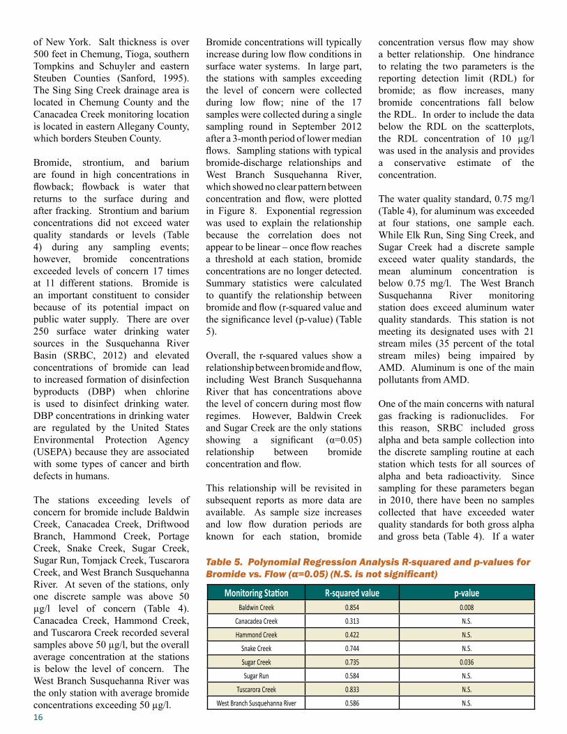
Table 5. Polynomial Regression Analysis R-squared and p-values for Bromide vs. Flow (α=0.05) (N.S. is not significant)

of New York. Salt thickness is over 500 feet in Chemung, Tioga, southern Tompkins and Schuyler and eastern Steuben Counties (Sanford, 1995). The Sing Sing Creek drainage area is located in Chemung County and the Canacadea Creek monitoring location is located in eastern Allegany County, which borders Steuben County.

Bromide, strontium, and barium are found in high concentrations in flowback; flowback is water that returns to the surface during and after fracking. Strontium and barium concentrations did not exceed water quality standards or levels (Table 4) during any sampling events; however, bromide concentrations exceeded levels of concern 17 times at 11 different stations. Bromide is an important constituent to consider because of its potential impact on public water supply. There are over 250 surface water drinking water sources in the Susquehanna River Basin (SRBC, 2012) and elevated concentrations of bromide can lead to increased formation of disinfection byproducts (DBP) when chlorine is used to disinfect drinking water. DBP concentrations in drinking water are regulated by the United States Environmental Protection Agency (USEPA) because they are associated with some types of cancer and birth defects in humans.

The stations exceeding levels of concern for bromide include Baldwin Creek, Canacadea Creek, Driftwood Branch, Hammond Creek, Portage Creek, Snake Creek, Sugar Creek, Sugar Run, Tomjack Creek, Tuscarora Creek, and West Branch Susquehanna River. At seven of the stations, only one discrete sample was above 50 µg/l level of concern (Table 4). Canacadea Creek, Hammond Creek, and Tuscarora Creek recorded several samples above 50 µg/l, but the overall average concentration at the stations is below the level of concern. The West Branch Susquehanna River was the only station with average bromide concentrations exceeding 50 µg/l.

Bromide concentrations will typically increase during low flow conditions in surface water systems. In large part, the stations with samples exceeding the level of concern were collected during low flow; nine of the 17 samples were collected during a single sampling round in September 2012 after a 3-month period of lower median flows. Sampling stations with typical bromide-discharge relationships and West Branch Susquehanna River, which showed no clear pattern between concentration and flow, were plotted in Figure 8. Exponential regression was used to explain the relationship because the correlation does not appear to be linear – once flow reaches a threshold at each station, bromide concentrations are no longer detected. Summary statistics were calculated to quantify the relationship between bromide and flow (r-squared value and the significance level (p-value) (Table 5).

Overall, the r-squared values show a relationship between bromide and flow, including West Branch Susquehanna River that has concentrations above the level of concern during most flow regimes. However, Baldwin Creek and Sugar Creek are the only stations showing a significant (α=0.05) relationship between bromide concentration and flow.

This relationship will be revisited in subsequent reports as more data are available. As sample size increases and low flow duration periods are known for each station, bromide

concentration versus flow may show a better relationship. One hindrance to relating the two parameters is the reporting detection limit (RDL) for bromide; as flow increases, many bromide concentrations fall below the RDL. In order to include the data below the RDL on the scatterplots, the RDL concentration of 10 µg/l was used in the analysis and provides a conservative estimate of the concentration.

The water quality standard, 0.75 mg/l (Table 4), for aluminum was exceeded at four stations, one sample each. While Elk Run, Sing Sing Creek, and Sugar Creek had a discrete sample exceed water quality standards, the mean aluminum concentration is below 0.75 mg/l. The West Branch Susquehanna River monitoring station does exceed aluminum water quality standards. This station is not meeting its designated uses with 21 stream miles (35 percent of the total stream miles) being impaired by AMD. Aluminum is one of the main pollutants from AMD.

One of the main concerns with natural gas fracking is radionuclides. For this reason, SRBC included gross alpha and beta sample collection into the discrete sampling routine at each station which tests for all sources of alpha and beta radioactivity. Since sampling for these parameters began in 2010, there have been no samples collected that have exceeded water quality standards for both gross alpha and gross beta (Table 4). If a water

17

Figure 8. Scatterplot Showing Non-linear Relationships between Bromide vs. Flow

Monitoring Station R-squared value p-valueBaldwin Creek 0.854 0.008

Canacadea Creek 0.313 N.S.

Hammond Creek 0.422 N.S.

Snake Creek 0.744 N.S.

Sugar Creek 0.735 0.036

Sugar Run 0.584 N.S.

Tuscarora Creek 0.833 N.S.

West Branch Susquehanna River 0.586 N.S.

Figure 9 shows the chemical diversity of the RWQMN stations. The NAPU ecoregion shows the least diversity as

seen by the red squares. The cations and anions are grouped together indicating similar water chemistry.

sample were to exceed water quality standards for gross alpha or beta, SRBC would investigate further for specific radionuclides.

The major anion (bicarbonate and carbonate, sulfate, and chloride) and cation (sodium and potassium, calcium, and magnesium) structure were plotted as percentages for each monitoring location and grouped by ecoregion using a Piper Diagram. A Piper Diagram displays the chemical characteristics of each station on one diagram, allowing for visual comparison. The cations are plotted on the left triangle while anions are plotted on the right triangle. The points on the two triangles are projected upward into the diamond until they intersect to visually show difference of ion chemistry between stations and ecoregions (University of Idaho, 2001).

Figure 9. RWQMN Piper Diagram

Outlier Stations

1. Trout Run

2. East Branch Fishing Creek

3. Baker Run

4. Kitchen Creek

5. Moose Creek

Ecoregion North Central Appalachian

Northern Appalachian Plateau

and Uplands

Central Appalachians Ridges

and Valleys

12

3

45

18

The Ridges and Valleys ecoregion stations show some diversity in the water chemistry. The cations plot close together, but there is a range in the anion percentages. Overall, the stations in this ecoregion do not plot in one tight group. The limited number of stations in the ecoregion and pollutant sources mentioned in the Monitoring Station Background section most likely contribute to this as more stations would potentially fill in the gaps between as seen in the other two ecoregions.

Within the NCA ecoregion, the anion structure shows a large diversity with the stations scattered throughout the anion plot. However, the cation structures are similar with the exception of Moose Creek and Kitchen Creek. These two stations have lower percentages of calcium and higher percentages of sodium and potassium when compared to the other stations in the NCA ecoregion. The use of road salt in Moose Creek and Kitchen Creek may lead to the difference in cation structure.

Road salt (NaCl) has been used as a road deicer in the northeastern United States since World War II; during runoff events, NaCl makes its way into surface water systems. Several watersheds in the network, including Moose Creek and Kitchen Creek, have major state roads and/or interstates passing through the watershed upstream of the monitoring station. Chloride/bromide ratios can be used to determine if road salt is the source of increased chloride and

sodium (Johnson, 2014). Typically, water impacted by road salt will have a chloride/bromide ratio between 1000 and 10,000 (Davis et al., 1998; Panno et al., 2006). Seven stations in the RWQMN have mean chloride/bromide ratios above 1000 (Table 6); Moose Creek is the only station in the NCA with a ratio over 1000.

Seventy percent and 50 percent of the cation structures of Moose Creek and Kitchen Creek, respectively, are comprised of sodium and potassium. Sodium and potassium percentages range from 10 to 35 percent in the remaining stations in the NCA ecoregion. Moose Creek and Kitchen Creek also have the largest percentages of chloride in the anion structure (80 and 50 percent, respectively).

Moose Creek is a predominantly forested watershed (95 percent) that is bordered by Interstate 80. Interstate 80 is a main corridor in northern

Station Chloride/Bromide Ratio EcoregionMoose Creek 2747 NCA

Sing Sing Creek 2209 NAPU

Canacadea Creek 1625 NAPU

South Branch Tunkhannock Creek 1361 NAPU

Trout Brook 1351 NAPU

Baldwin Creek 1230 NAPU

Nanticoke Creek 1025 NAPU

Table 6. Mean Chloride/Bromide Ratio in Road Salt Impacted Watersheds

Pennsylvania; road salt is the primary deicer applied to roads during freezing precipitation events. Each discrete sampling event conducted on Moose Creek in which chloride and bromide were detected, the chloride/bromide ratio is over 1000, for an average ratio of 2747.

Kitchen Creek also shows a different cation structure from the other stations in the NCA ecoregion; however, bromide was only detected once above the RDL (10 µg/l). With the limited number of bromide samples above the RDL, the chloride/bromide ratio cannot be used to determine the source of chloride. Six stations in the NAPU ecoregion have chloride/bromide ratios that indicate road salt as a source of chloride. These stations are not outliers in the cation structure as there are more stations impacted compared to the NCA ecoregion and there are other potential sources of salt, such as brine.

When the anion and cation percentages are combined in the quadrilateral, the majority of the stations group together, leaving only five stations as outliers. These stations include Baker Run, Kitchen Creek, Moose Creek, Trout Run, and East Branch Fishing Creek. The water quality at these sites is not poor or degraded, just the anion/cation composition did not group well with other streams in the ecoregion.

Moose Creek, Clearfield County, Pa.

19

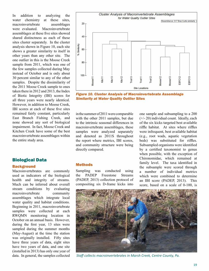
In addition to analyzing the water chemistry at these sites, macroinvertebrate assemblages were evaluated. Macroinvertebrate assemblages at these five sites showed shared distinctness as each of these sites cluster separately. In the cluster analysis shown in Figure 10, each site shows a greater similarity to itself in other years than any other site. The one outlier in this is the Moose Creek sample from 2011, which was one of the few samples collected during May instead of October and is only about 30 percent similar to any of the other samples. Despite the dissimilarity of the 2011 Moose Creek sample to ones taken there in 2012 and 2013, the Index of Biotic Integrity (IBI) scores for all three years were nearly identical. However, in addition to Moose Creek, IBI scores at each of these five sites remained fairly constant, particularly East Branch Fishing Creek, and none showed any sort of biological impairment. In fact, Moose Creek and Kitchen Creek have some of the best macroinvertebrate assemblages within the entire study area.

Figure 10. Cluster Analysis of Macroinvertebrate Assemblage Similarity at Water Quality Outlier Sites

Biological DataBackgroundMacroinvertebrates are commonly used as indicators of the biological health and integrity of streams. Much can be inferred about overall stream conditions by evaluating macroinvertebrate community assemblages which integrate local water quality and habitat conditions. Beginning in 2011, macroinvertebrate samples were collected at each RWQMN monitoring location in October on an annual basis. However, during the first year, 13 sites were sampled during the summer months (May-August) at the time the station was originally installed. Fifty sites have three years of data, eight sites have two years of data, and one site (installed in 2013) has only one year of data. In general, the samples collected

in the summer of 2011 were comparable with the other 2011 samples, but due to the intrinsic seasonal differences in macroinvertebrate assemblages, these samples were analyzed separately and denoted as 2011S throughout the report where metrics, IBI scores, and community structure were being directly compared.

MethodsSampling was conducted using the PADEP Freestone Streams (PADEP, 2013) collection protocol of compositing six D-frame kicks into

one sample and subsampling to a 200 (+/- 20) individual count. Ideally, each of the six kicks targeted best available riffle habitat. At sites where riffles were infrequent, best available habitat (e.g., root wads, aquatic vegetation beds) was substituted for riffles. Subsampled organisms were identified by a certified taxonomist to genus when possible, with the exception of Chironomidae, which remained at family level. The taxa identified in the subsample were scored through a number of individual metrics which were combined to determine an IBI score (PADEP, 2013). This score, based on a scale of 0-100, is

Staff collects macroinvertebrates in Marsh Creek, Centre County, Pa.

20

Metric Explanation

Taxa RichnessA count of the total number of taxa in a sub-sample. This metric is expected to decrease with increasing anthropogenic stress to a stream ecosystem, reflecting loss of taxa and increasing dominance of a few pollution-tolerant taxa.

EPT Taxa (PTV 0-4)

A count of the number of taxa belonging to the orders Ephemeroptera, Plecoptera, and Trichoptera (EPT) in a sub-sample. This version of the EPT metric only counts EPT taxa with Pollution Tolerance Values (PTVs) of 0 to 4. This metric is expected to decrease in value with increasing anthropogenic stress to a stream ecosystem.

Becks Index (version 3)A weighted count of taxa with PTVs of 0, 1, or 2. This metric is expected to decrease in value with increasing anthropogenic stress to a stream ecosystem, reflecting the loss of pollution-sensitive taxa.

Shannon Diversity

A measure of taxonomic richness and evenness of individuals across taxa in a sub-sample. This metric is expected to decrease in value with increasing anthropogenic stress to a stream ecosystem, reflecting loss of pollution-sensitive taxa and increasing dominance pollution-tolerant taxa.

Hilsenhoff Biotic IndexThis community composition and tolerance metric is an average of the number of individuals in a sub-sample, weighted by PTVs. Generally increases with increasing ecosystem stress, reflecting increasing dominance of pollution-tolerant taxa.

Percent Sensitive Individuals (PTV 0-3)

This community composition and tolerance metric is the percentage of individuals with PTVs of 0 to 3 in a sub-sample and is expected to decrease in value with increas-ing anthropogenic stress to a stream ecosystem, reflecting loss of pollution-sensitive organisms.

Table 7. Explanation of Individual Metrics Comprising PA IBI (PADEP, 2013)a representation of the quality of the macroinvertebrate assemblage based on six separate metrics which describe different aspects of the community. Table 7 gives an explanation for each of these metrics and the expected response as a result of increasing anthropogenic stress.

Two different approaches were used to analyze the biological data. One approach relied primarily on the IBI score, which is useful in combining some of the most discriminatory metrics into a single number for easy comparison across sites and also takes into account index period and stream size. However, there are drawbacks to simply using an IBI score, as dissimilar communities can have comparable IBI scores. The second analysis approach is based on community similarity and uses numerous statistical tools that are centered around the Bray-Curtis similarity matrix.

IBI scores are a helpful starting place when evaluating macroinvertebrate communities, but the identification of what metrics or even specific taxa are driving those IBI scores is important. For instance, within the IBI framework, Pollution Tolerance Values (PTVs) are assigned by genera and reflect an organism’s susceptibility to organic pollution; examples of organic pollution include wastewater effluent, runoff from agricultural lands, and discharges from manufacturing processes. One of the drawbacks of relying on PTVs is that PTVs do not account for other sources of stream impairments. For example, a stream may have acidic conditions due to AMD pollution. The resulting macroinvertebrate assemblage may contain many acid-tolerant stoneflies that have low PTV scores, which will inflate the IBI score despite the impaired water quality conditions. Similarly, sedimentation often goes hand-in-hand with some forms of organic pollution, but in cases where it does not, PTVs may not always accurately reflect any tolerance to sediment or increased turbidity.

Identifying specific genera that may be abundant in a subsample and asserting a dominance effect on the IBI score is helpful to interpreting the score. A dominance of one sensitive taxa with a low PTV can inflate an IBI score by impacting four of the six metrics. When one genus dominates a sample in any one year, the comparability of the data across all years can be compromised. In the same manner, a one-time dominance of a tolerant taxa within the subsample can cause a drop

in IBI score that may not be indicative of actual conditions.

For this analysis, a combination of IBI scores, discrete metrics, and non-parametric statistical methods will be used to identify spatial and temporal patterns within the data and evaluate potential factors behind these patterns. In addition, relationships between macroinvertebrate communities and unconventional gas drilling activity will be explored.

Staff processes macroinvertebrates in Baker Run, Clinton County, Pa.

21

Results and Discussion

A majority of the watersheds within the RWQMN are in fairly undeveloped areas where streams consist of sufficient habitat and water quality to support a healthy macroinvertebrate assemblage. The average forest coverage in RWQMN watersheds is 74 percent, with a minimum of 35 percent (Sangerfield River) and a maximum of 99 percent (Baker Run). Of all samples taken over the three years, less than 6 percent of samples scored as impaired using the PA IBI. These ten impaired samples were from seven different sites, and many of the sites scored just above the impairment line in other years. Sites with poor IBI scores in more than one year were Hammond Creek, Trout Brook, West Branch Susquehanna River, Chest Creek, Canacadea Creek, and Sugar Creek. These sites also scored consistently low on the habitat assessment, with most years falling in the lower 25th percentile of all Rapid Bioassessment Protocol (RBP) habitat scores. Severe erosion, lack of stream cover, infrequent riffle-run habitat units, and excessive algal growth create sub-optimal conditions for macroinvertebrate assemblages at these sites. Although not a strong correlation, overall RBP habitat score is positively and significantly correlated with IBI score (Pearson r=0.419, p<0.05). Having less-than-optimal habitat scores correlate with impaired macroinvertebrate assemblages is not surprising.

Comparison of IBI Scores Across YearsCalculated IBI scores for each site were compared to evaluate differences in IBI scores between sampling periods. A Kruskall-Wallis test was used to determine there was a difference between IBI scores across sampling periods: 2011S, 2011, 2012, and 2013 (p=0.002). By examining the associated z scores, the summer 2011 summer samples were the most

different from the other sampling periods, as could be expected due to natural seasonal variation between summer and October. Figure 11 shows a boxplot of the results for differences in IBI score across the temporal range as well as sample size for each group.

To determine which specific sampling periods were significantly different

Figure 11. Macroinvertebrate Index of Biotic Integrity (IBI) Scores at Remote Water Quality Monitoring Stations from 2011 to 2013

(α=0.05) from each other, a Mann-Whitney test was used for each combination (Table 8). The 2011S sampling period was significantly different from all other sampling periods and 2011 was also significantly different from 2012. Again, this is not unexpected given the seasonal influences on macroinvertebrate assemblages.

IBI(Mann-Whitney)

Community Similarity (ANOSIM)

Comparative groups p-value p-value

2011S vs. 2011 0.049 0.001

2011S vs. 2012 0.003 0.001

2011S vs. 2013 0.009 0.001

2011 vs. 2012 0.040 0.001

2011 vs. 2013 N.S. 0.001

2012 vs. 2013 N.S. 0.001

Table 8. Summary Results of Significance (α=0.05) Testing Between Sampling Periods (N.S. is not significant)

n=13 n=37 n=58 n=59

Of all [biological] samples taken over the three years, less than 6 percent of the sampled scored

as impaired using the PA IBI.

22

IBI(Mann-Whitney) Community Similarity (ANOSIM)

Comparative groups p-value p-value

NAPU vs NCA < 0.001 0.001

NAPU vs RV N.S. N.S.

NCA vs RV <0.001 0.006

Comparison of Community Similarity Between YearsBecause it is possible for dissimilar macroinvertebrate assemblages to have similar IBI scores, the ANOSIM function within the PRIMER-E software package was used to indicate significant differences between assemblage factors based on the Bray-Curtis similarity matrix. Essentially, ANOSIM is an ANOVA constructed from similarity values between biological communities. The results from the ANOSIM between sampling periods for community similarity showed a significant difference (p=0.001) among all years even though the IBI scores between 2011 and 2013 and 2012 and 2013 were not significantly different (Table 8). This confirms differences in macroinvertebrate community structure even if IBI scores are comparable.

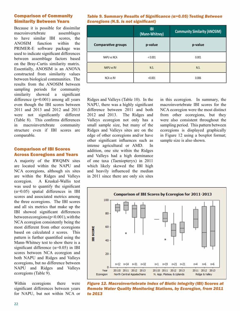
Comparison of IBI Scores Across Ecoregions and YearsA majority of the RWQMN sites are located within the NAPU and NCA ecoregions, although six sites are within the Ridges and Valleys ecoregion. A Kruskal-Wallis test was used to quantify the significant (α=0.05) spatial differences in IBI scores and associated metrics among the three ecoregions. The IBI scores and all six metrics that make up the IBI showed significant differences between ecoregions (p<0.001), with the NCA ecoregion consistently being the most different from other ecoregions based on calculated z scores. This pattern is further quantified using the Mann-Whitney test to show there is a significant difference (α=0.05) in IBI scores between NCA ecoregion and both NAPU and Ridges and Valleys ecoregions, but no difference between NAPU and Ridges and Valleys ecoregions (Table 9).

Within ecoregions there were significant differences between years for NAPU, but not within NCA or

Table 9. Summary Results of Significance (α=0.05) Testing Between Ecoregions (N.S. is not significant)

Figure 12. Macroinvertebrate Index of Biotic Integrity (IBI) Scores at Remote Water Quality Monitoring Stations, by Ecoregion, from 2011 to 2013

Ridges and Valleys (Table 10). In the NAPU, there was a highly significant difference between 2011 and both 2012 and 2013. The Ridges and Valleys ecoregion not only has a small sample size, but many of the Ridges and Valleys sites are on the edge of other ecoregions and/or have other significant influences such as intense agricultural or AMD. In addition, one site within the Ridges and Valleys had a high dominance of one taxa (Taeniopteryx) in 2011 which likely skewed the IBI high and heavily influenced the median in 2011 since there are only six sites

in this ecoregion. In summary, the macroinvertebrate IBI scores for the NCA ecoregion were the most distinct from other ecoregions, but they were also consistent throughout the sampling period. This pattern between ecoregions is displayed graphically in Figure 12 using a boxplot format; sample size is also shown.

n=12 n=14 n=31 n=32 n=1 n=19 n=21 n=21 n=4 n=6 n=6

23

Comparison of Community Similarity Across Ecoregions and Years

ANOSIM analysis indicated that community assemblages were also significantly different in the NCA when compared to both other ecoregions but that there was no significant difference between NAPU and Ridges and Valleys. However, the pairwise analysis of community similarity between years revealed significant differences that were not evident by only using IBI scores. Within the NAPU, which has the most obvious differences in spread of data and non-overlapping interquartile ranges (see Figure 12), the results were the same but within NCA and Ridges and Valleys, other significant differences are seen (Table 8). The NCA shows significant assemblages differences between each sampling period although the IBI scores are not significantly different.

NCA NAPU RV

IBI Score(Mann-Whitney)

Community Similarity (ANOSIM)

IBI Score (Mann-Whitney)

Community Similarity (ANOSIM)

IBI Score(Mann-Whitney)

Community Similarity (ANOSIM)

2011S vs 2011 N.S 0.002 --- --- --- ---

2011S vs 2012 N.S 0.001 --- --- --- ---

2011S vs 2013 N.S 0.001 --- --- --- ---

2011 vs 2012 N.S 0.016 < 0.001 0.001 N.S. N.S.

2012 vs 2013 N.S 0.001 N.S. N.S. N.S. N.S.

2011 vs 2013 N.S 0.001 0.001 0.001 N.S. 0.024

Table 10. Summary Results Of Significance Testing (α=0.05) Between Years Within Ecoregion (N.S. is not significant)

The macroinvertebrate IBI scores for the NCA ecoregion

are the most distinct from other ecoregions, but they are also consistent throughout the

sampling period.

Staff processes fish sampled along Little Pine Creek, Lycoming County, Pa.

Staff measures brown trout captured in East Fork Sinnemahoning Creek, Potter County, Pa.

24

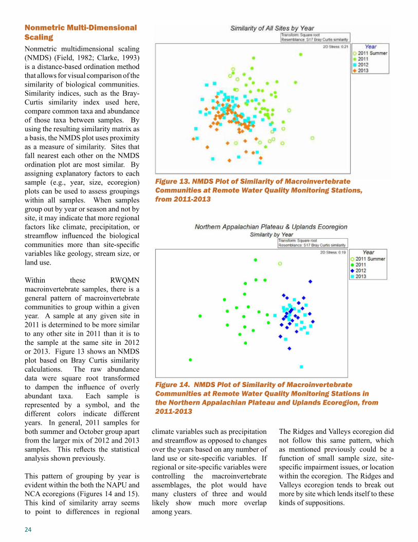
Nonmetric Multi-Dimensional ScalingNonmetric multidimensional scaling (NMDS) (Field, 1982; Clarke, 1993) is a distance-based ordination method that allows for visual comparison of the similarity of biological communities. Similarity indices, such as the Bray-Curtis similarity index used here, compare common taxa and abundance of those taxa between samples. By using the resulting similarity matrix as a basis, the NMDS plot uses proximity as a measure of similarity. Sites that fall nearest each other on the NMDS ordination plot are most similar. By assigning explanatory factors to each sample (e.g., year, size, ecoregion) plots can be used to assess groupings within all samples. When samples group out by year or season and not by site, it may indicate that more regional factors like climate, precipitation, or streamflow influenced the biological communities more than site-specific variables like geology, stream size, or land use.

Within these RWQMN macroinvertebrate samples, there is a general pattern of macroinvertebrate communities to group within a given year. A sample at any given site in 2011 is determined to be more similar to any other site in 2011 than it is to the sample at the same site in 2012 or 2013. Figure 13 shows an NMDS plot based on Bray Curtis similarity calculations. The raw abundance data were square root transformed to dampen the influence of overly abundant taxa. Each sample is represented by a symbol, and the different colors indicate different years. In general, 2011 samples for both summer and October group apart from the larger mix of 2012 and 2013 samples. This reflects the statistical analysis shown previously.

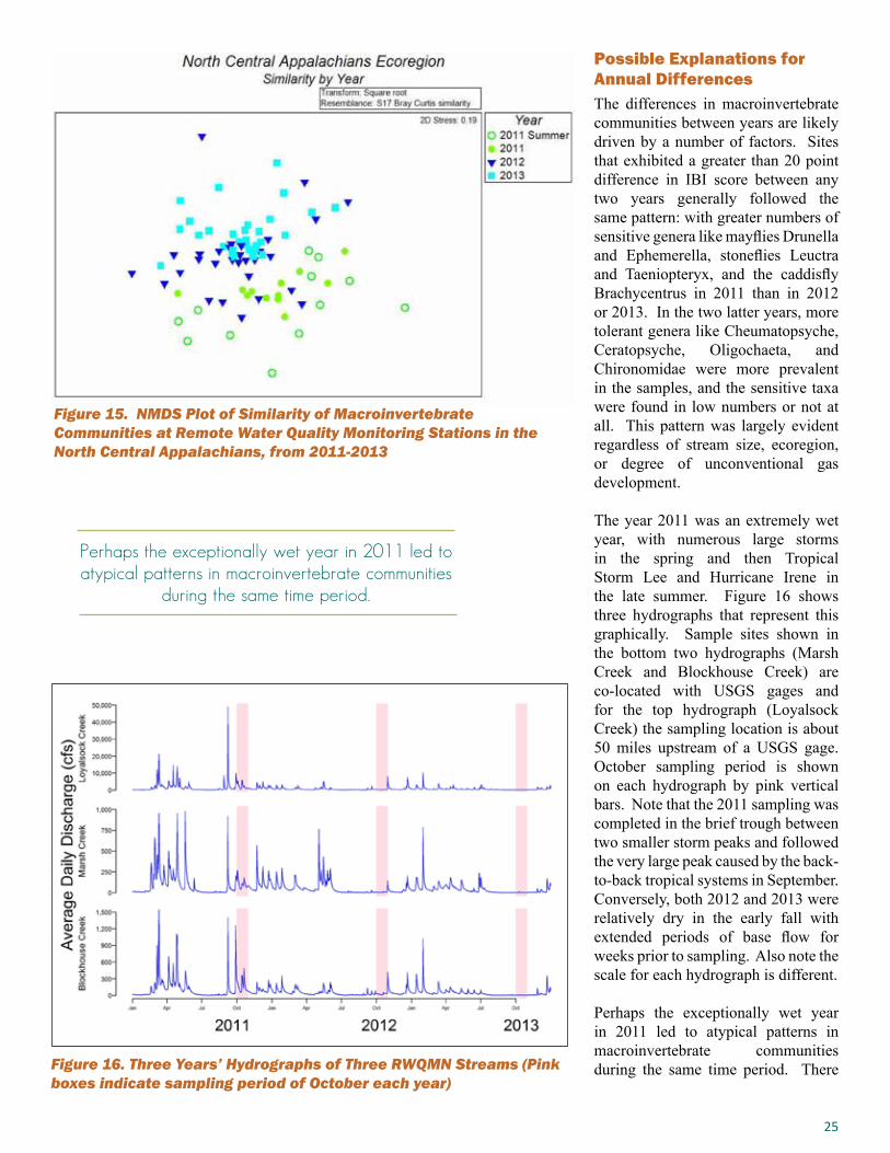
This pattern of grouping by year is evident within the both the NAPU and NCA ecoregions (Figures 14 and 15). This kind of similarity array seems to point to differences in regional

climate variables such as precipitation and streamflow as opposed to changes over the years based on any number of land use or site-specific variables. If regional or site-specific variables were controlling the macroinvertebrate assemblages, the plot would have many clusters of three and would likely show much more overlap among years.

Figure 13. NMDS Plot of Similarity of Macroinvertebrate Communities at Remote Water Quality Monitoring Stations, from 2011-2013

The Ridges and Valleys ecoregion did not follow this same pattern, which as mentioned previously could be a function of small sample size, site-specific impairment issues, or location within the ecoregion. The Ridges and Valleys ecoregion tends to break out more by site which lends itself to these kinds of suppositions.

Figure 14. NMDS Plot of Similarity of Macroinvertebrate Communities at Remote Water Quality Monitoring Stations in the Northern Appalachian Plateau and Uplands Ecoregion, from 2011-2013

25

Figure 15. NMDS Plot of Similarity of Macroinvertebrate Communities at Remote Water Quality Monitoring Stations in the North Central Appalachians, from 2011-2013

Possible Explanations for Annual Differences The differences in macroinvertebrate communities between years are likely driven by a number of factors. Sites that exhibited a greater than 20 point difference in IBI score between any two years generally followed the same pattern: with greater numbers of sensitive genera like mayflies Drunella and Ephemerella, stoneflies Leuctra and Taeniopteryx, and the caddisfly Brachycentrus in 2011 than in 2012 or 2013. In the two latter years, more tolerant genera like Cheumatopsyche, Ceratopsyche, Oligochaeta, and Chironomidae were more prevalent in the samples, and the sensitive taxa were found in low numbers or not at all. This pattern was largely evident regardless of stream size, ecoregion, or degree of unconventional gas development.

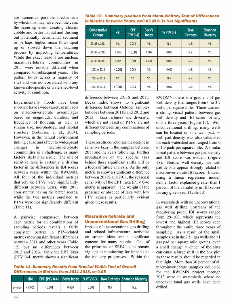
The year 2011 was an extremely wet year, with numerous large storms in the spring and then Tropical Storm Lee and Hurricane Irene in the late summer. Figure 16 shows three hydrographs that represent this graphically. Sample sites shown in the bottom two hydrographs (Marsh Creek and Blockhouse Creek) are co-located with USGS gages and for the top hydrograph (Loyalsock Creek) the sampling location is about 50 miles upstream of a USGS gage. October sampling period is shown on each hydrograph by pink vertical bars. Note that the 2011 sampling was completed in the brief trough between two smaller storm peaks and followed the very large peak caused by the back-to-back tropical systems in September. Conversely, both 2012 and 2013 were relatively dry in the early fall with extended periods of base flow for weeks prior to sampling. Also note the scale for each hydrograph is different.

Perhaps the exceptionally wet year in 2011 led to atypical patterns in macroinvertebrate communities during the same time period. There Figure 16. Three Years’ Hydrographs of Three RWQMN Streams (Pink

boxes indicate sampling period of October each year)

Perhaps the exceptionally wet year in 2011 led to atypical patterns in macroinvertebrate communities

during the same time period.

26

are numerous possible mechanisms by which this may have been the case: the scouring event creating cleaner cobble and better habitat and flushing out potentially detrimental sediment or perhaps higher mean flows sped up or slowed down the hatching process by impacting temperatures. While the exact reasons are unclear, macroinvertebrate communities in 2011 were notably different when compared to subsequent years. The pattern holds across a majority of sites and was not correlated with any known site-specific or watershed-level activity or condition.

Experimentally, floods have been shown to have a wide variety of impacts on macroinvertebrate assemblages based on magnitude, duration, and frequency of flooding, as well as stream size, morphology, and habitat structure (Robinson et al., 2004). However, in the natural environment linking cause and effect to widespread changes in macroinvertebrate communities is a challenge, as many factors likely play a role. The role of sensitive taxa is certainly a driving factor in the differences in IBI scores between years within the RWQMN. All four of the individual metrics that rely on PTVs were significantly different between years, with 2011 consistently having the better scores, while the two metrics unrelated to PTVs were not significantly different (Table 11).

A pairwise comparison between each metric for all combinations of sampling periods reveals a fairly consistent pattern in PTV-related metrics showing significant differences between 2011 and other years (Table 12) but no differences between 2012 and 2013. Only the EPT Taxa (PTV 0-4) metric shows a significant

difference between 2011S and 2011. Becks Index shows no significant difference between October samples but does between 2011S and 2012 and 2013. Taxa richness and diversity, which are not based on PTVs, are not different between any combinations of sampling periods.

These results corroborate the decline in sensitive taxa in the samples between 2011 and the years following. Further investigation of the specific taxa behind these significant shifts will be a focus of future analysis. As the only metric to show a significant difference between 2011S and 2011, the seasonal sensitivity of the EPT Taxa (PTV 0-4) metric is apparent. The weight of the presence or absence of taxa with low PTV values is particularly evident given these results.

Table 11. Summary Results from Kruskal-Wallis Test of Overall Differences in Metrics from 2011-2013, α=0.05

HBI EPT (PTV 0-4) Becks Index % PTV 0-3 Taxa Richness Shannon Diversity

p-value < 0.001 < 0.001 0.029 < 0.001 N.S. N.S.

Comparative Groups HBI EPT

(PTV 0-4)Beck’s Index % PTV 0-3 Taxa

RichnessShannon Diversity

2011S vs 2011 N.S. 0.034 N.S. N.S. N.S. N.S.

2011S vs 2012 0.006 < 0.001 0.006 0.007 N.S. N.S.

2011S vs 2013 0.002 0.001 0.040 0.003 N.S. N.S.

2011 vs 2012 < 0.001 0.004 N.S. 0.001 N.S. N.S.

2012 vs 2013 N.S. N.S. N.S. N.S. N.S. N.S.

2011 vs 2013 < 0.001 0.034 N.S. 0.001 N.S. N.S.

Table 12. Summary p-values from Mann-Whitney Test of Differences in Metrics Between Years, α=0.05 (N.S. is Not Significant)

Macroinvertebrate and Unconventional Gas Drilling Impacts of unconventional gas drilling and related infrastructural activities on stream biota are a significant concern for many people. One of the priorities of SRBC is to remain vigilant in monitoring for impacts as the industry progresses. Within the

RWQMN, there is a gradient of gas well density that ranges from 0 to 3.7 wells per square mile. There was not a strong visual pattern between gas well density and IBI score for any of the three years (Figure 17). With unconventional drilling, many wells can be located on one well pad, so well pad density was also calculated for each watershed and ranged from 0 to 1.3 pads per square mile. A similar visual pattern between gas pad density and IBI score was evident (Figure 18). Neither well density nor well pad density appear strongly related to macroinvertebrate IBI score. Indeed, using a linear regression model, neither factor explained greater than 1 percent of the variability in IBI scores for any given year (Table 13).

In watersheds with no unconventional gas well drilling upstream of the monitoring point, IBI scores ranged from 29–100, which represents the lowest and highest IBI scores seen throughout the entire three years of sampling. As a result of the small sample size in the 2.5+ gas wells and >1 gas pad per square mile groups, even a small change at either of the sites can cause a large shift in the box plot so those results should be regarded in that light. More than 30 percent of all macroinvertebrate samples collected for the RWQMN project through 2013 were in watersheds where no unconventional gas wells have been drilled.

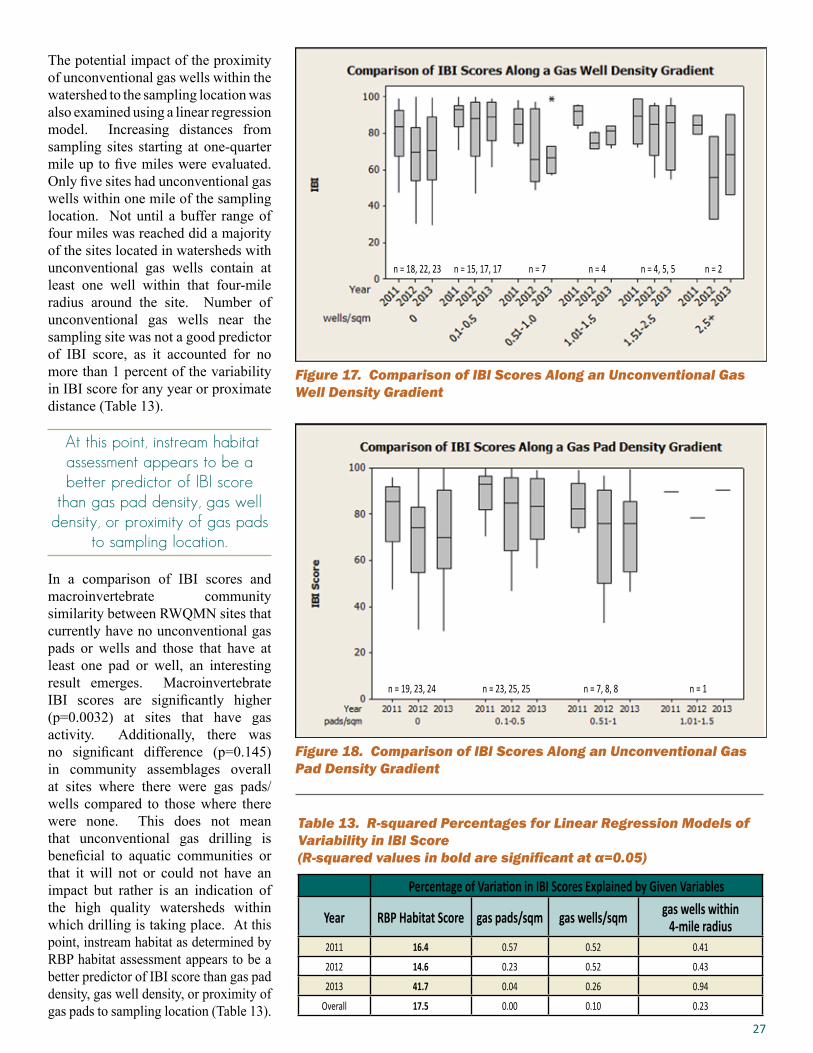
27

Figure 17. Comparison of IBI Scores Along an Unconventional Gas Well Density Gradient

Figure 18. Comparison of IBI Scores Along an Unconventional Gas Pad Density Gradient

Percentage of Variation in IBI Scores Explained by Given Variables

Year RBP Habitat Score gas pads/sqm gas wells/sqm gas wells within 4-mile radius

2011 16.4 0.57 0.52 0.41

2012 14.6 0.23 0.52 0.43

2013 41.7 0.04 0.26 0.94

Overall 17.5 0.00 0.10 0.23

Table 13. R-squared Percentages for Linear Regression Models of Variability in IBI Score(R-squared values in bold are significant at α=0.05)

The potential impact of the proximity of unconventional gas wells within the watershed to the sampling location was also examined using a linear regression model. Increasing distances from sampling sites starting at one-quarter mile up to five miles were evaluated. Only five sites had unconventional gas wells within one mile of the sampling location. Not until a buffer range of four miles was reached did a majority of the sites located in watersheds with unconventional gas wells contain at least one well within that four-mile radius around the site. Number of unconventional gas wells near the sampling site was not a good predictor of IBI score, as it accounted for no more than 1 percent of the variability in IBI score for any year or proximate distance (Table 13).

In a comparison of IBI scores and macroinvertebrate community similarity between RWQMN sites that currently have no unconventional gas pads or wells and those that have at least one pad or well, an interesting result emerges. Macroinvertebrate IBI scores are significantly higher (p=0.0032) at sites that have gas activity. Additionally, there was no significant difference (p=0.145) in community assemblages overall at sites where there were gas pads/wells compared to those where there were none. This does not mean that unconventional gas drilling is beneficial to aquatic communities or that it will not or could not have an impact but rather is an indication of the high quality watersheds within which drilling is taking place. At this point, instream habitat as determined by RBP habitat assessment appears to be a better predictor of IBI score than gas pad density, gas well density, or proximity of gas pads to sampling location (Table 13).

n = 18, 22, 23 n = 15, 17, 17 n = 7 n = 4 n = 2n = 4, 5, 5

n = 19, 23, 24 n = 23, 25, 25 n = 7, 8, 8 n = 1

At this point, instream habitat assessment appears to be a better predictor of IBI score

than gas pad density, gas well density, or proximity of gas pads

to sampling location.

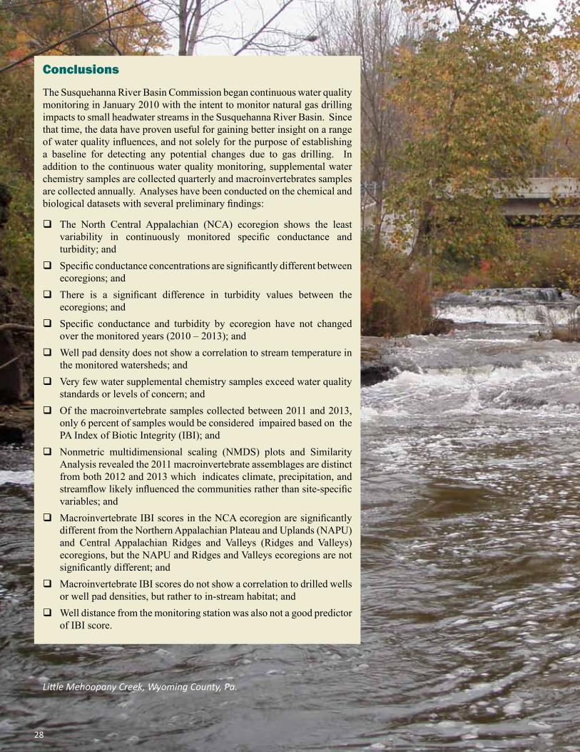
Conclusions

The Susquehanna River Basin Commission began continuous water quality monitoring in January 2010 with the intent to monitor natural gas drilling impacts to small headwater streams in the Susquehanna River Basin. Since that time, the data have proven useful for gaining better insight on a range of water quality influences, and not solely for the purpose of establishing a baseline for detecting any potential changes due to gas drilling. In addition to the continuous water quality monitoring, supplemental water chemistry samples are collected quarterly and macroinvertebrates samples are collected annually. Analyses have been conducted on the chemical and biological datasets with several preliminary findings:

� The North Central Appalachian (NCA) ecoregion shows the least variability in continuously monitored specific conductance and turbidity; and

� Specific conductance concentrations are significantly different between ecoregions; and

� There is a significant difference in turbidity values between the ecoregions; and

� Specific conductance and turbidity by ecoregion have not changed over the monitored years (2010 – 2013); and

� Well pad density does not show a correlation to stream temperature in the monitored watersheds; and

� Very few water supplemental chemistry samples exceed water quality standards or levels of concern; and

� Of the macroinvertebrate samples collected between 2011 and 2013, only 6 percent of samples would be considered impaired based on the PA Index of Biotic Integrity (IBI); and

� Nonmetric multidimensional scaling (NMDS) plots and Similarity Analysis revealed the 2011 macroinvertebrate assemblages are distinct from both 2012 and 2013 which indicates climate, precipitation, and streamflow likely influenced the communities rather than site-specific variables; and

� Macroinvertebrate IBI scores in the NCA ecoregion are significantly different from the Northern Appalachian Plateau and Uplands (NAPU) and Central Appalachian Ridges and Valleys (Ridges and Valleys) ecoregions, but the NAPU and Ridges and Valleys ecoregions are not significantly different; and

� Macroinvertebrate IBI scores do not show a correlation to drilled wells or well pad densities, but rather to in-stream habitat; and

� Well distance from the monitoring station was also not a good predictor of IBI score.

28

Little Mehoopany Creek, Wyoming County, Pa.

Overall, the cation and anion structures from all the stations are similar with the exception of five stations in the NCA ecoregion. These stations exhibit good water chemistry, but show differences in the cation structure (Moose and Kitchen Creeks) and overall structure (Moose, Kitchen, and East Branch Fishing Creeks and Trout and Baker Runs). Macroinvertebrate communities were analyzed at these stations and no biological impairments were noted; in fact, these stations have some of the highest IBI scores.

A few incidents have occurred as a result of drilling activities upstream of select monitoring stations. In those cases, Pennsylvania agencies have used the continuous water chemistry data to track the events and determine if any water quality impacts occurred. In addition to other agencies using the continuous water chemistry data to track events, SRBC staff collects supplemental lab water chemistry data if significant deviations are seen in the continuous data. SRBC staff receives an email alert if continuously monitored parameters deviate from an established concentration range which prompts the use of established plans outlining protocols on where and how to collect water samples within the watershed. These data assist in determining the reason behind deviations in the continuous water chemistry data.

Impacts from construction, agricultural practices, development, climate change, and other activities influencing the continuously monitored water quality parameters and biological communities will be analyzed along with natural gas impacts as chemical and biological data continue to be collected by the Remote Water Quality Monitoring network. SRBC will continue to monitor the stations and provide a technical summary of all the data collected by the network, but future reports will begin to focus more on analysis of water chemistry by potential impacts, trend analyses of the continuous data, and more in-depth assessments of the biological data. In addition to SRBC analyzing the data, there are numerous agencies and universities using the data for research purposes and to study the impacts of climate change, road salt use, and natural gas impacts.

29

References

Clarke, K.R. 1993. Non-parametric multivariate analysis of changes in community structure. Australian Journal of Ecology, 18, 117-143.

Cornell Cooperative Extension – Ulster County, New York City Department of Environmental Protection, and U.S. Army Engineer Research Development Center. 2007. Upper Esopus Creek Management Plan. Volume I: Summary of Finding and Recommendations.

Davis, S.N, D.O. Whittemore, & J. Fabryka-Martin. 1998. Uses of Chloride/Bromide Ratios in Studies of Potable Water. Ground Water, Vol. 36, No. 2. 338 – 350.

Drohan, P.J, M. Brittingham, J. Bishop, & K. Yoder. 2012. Early Trends in Landcover Change and Forest Fragmentation Due to Shale-Gas Development in Pennsylvania: A Potential Outcome for the Northcentral Appalachians. Environmental Management. Springer Science+Business Media, LLC.

Field, J.G., K.R. Clarke, & R.M. Warwick. 1982. A practical strategy for analyzing multispecies distribution patterns. Marine Ecology Progress Series 8, 37-52.

Hintz, D. 2013. Remote Water Quality Monitoring Network, Data Report of Baseline Conditions for 2010 - 2012. Susquehanna River Basin Commission (Publication No. 292), Harrisburg, Pennsylvania.

_____. 2012. Remote Water Quality Monitoring Network, Data Report of Baseline Conditions for 2010/2011. Susquehanna River Basin Commission (Publication No. 280), Harrisburg, Pennsylvania.

Hirsch, R.M. 2012. Flux of nitrogen, phosphorus, and suspended sediment from the Susquehanna River Basin to the Chesapeake Bay during Tropical Storm Lee, September 2011, as an indicator of the effects of reservoir sedimentation on water quality: U.S. Geological Survey Scientific Investigations Report 2012–5185, 17 p.

Johnson, J. D. 2014. Unpublished. Coupling Geochemistry and Real-time Water Quality Sensing for Identifying and Quantifying Basin Brine and Road Salt Sources in Watersheds Along the New York Pennsylvania Border. Dissertation for Doctor of Philosophy in Geology in the Graduate School of Binghamton University State University of New York.

Missouri Department of Natural Resources. 2006. Water Quality in Missouri’s Larger Rivers. http://dnr.mo.gov/pubs/pub2020.pdf.

National Oceanic and Atmospheric Administration. 2012. Regional Assessment Remnants of Tropical Storm Lee and the Susquehanna River Basin Flooding of September 6-10, 2011. U.S. Department of Commerce. National Weather Service, Eastern Region Headquarters. Bohemia, NY. http://www.nws.noaa.gov/om/assessments/pdfs/LeeSusquehanna12.pdf.

New York State Department of Environmental Conservation. 2006. Standardized Biological Field Collection and Laboratory Methods. http://www.elibrary.dep.state.pa.us/dsweb/Get/Document-59743.

_____. 1999. §703.3 Water quality standards for pH, dissolved oxygen, dissolved solids, odor, color and turbidity. http://www.dec.ny.gov/regs/4590.html#16132.

Panno, S.V., et al. 2006. Characterization and Identification of Na-Cl Sources in Ground Water. Ground Water, Vol. 44, No. 2. 176-187.

Pennsylvania Department of Environmental Protection. 2014. 2014 Pennsylvania Integrated Water Quality Monitoring and Assessment Report. http://www.portal.state.pa.us/portal/server.pt/community/water_quality_standards/10556/draft_integrated_water_quality_report_-_2014/1702856.

30

_____. 2013. A Benthic Macroinvertebrate Index of Biotic Integrity for Wadeable Freestone Riffle--Run Streams in Pennsylvania. Pennsylvania Department of Environmental Protection. Division of Water Quality Standards.

_____. 2010. Chapter 93. Water Quality Standards. http://www.pacode.com/secure/data/025/chapter93/025_0093.pdf.

_____. 2006. Standardized Biological Field Collection and Laboratory Methods. http://www.elibrary.dep.state.pa.us/dsweb/Get/Document-59743.

Robinson, C., S. Aebischer, and U. Uehlinger. 2004. Immediate and habitat-specific responses of macroinvertebrates to sequential, experimental floods. Journal of the North American Benthological Society. 23:4 (853-867).

Rogers, W.B., Y.W. Isachsen, T.D Mock, and R.E. Nyahay. 1990. Overview of New York Geology. Adapted from Education Leaflet 33. http://gretchen.geo.rpi.edu/roecker/nys/nys_edu.pamphlet.html.

Sanford, K.F. 1995. New York State Department of Environmental Conservation, Division of Mineral Resources. Solution Salt Mining in New York. http://www.dec.ny.gov/docs/materials_minerals_pdf/ssmny96.pdf.

Sayler, Kristi L. 2014. United States Geological Survey, Center for Earth Resources and Observation and Science. Land Cover Trends Project – North Central Appalachian. http://landcovertrends.usgs.gov/east/eco62Report.html.

Susquehanna River Basin Commission. 2015. Hydra Database. Well Pad Approvals. January 2015.

_____. 2013. SRB_StForest. State Forest Lands. GIS shapefile.

_____. 2012. SRB_PWSSW_12.shp. Surface Water Drinking Sources. GIS shapefile.

United States Environmental Protection Agency. 2015. Water: Monitoring and Assessment. 5.5 Turbidity. http://water.epa.gov/type/rsl/monitoring/vms55.cfm.

_____. 2003. Office of Water. Drinking Water Advisory: Consumer Acceptability Advice and Health Effects Analysis on Sodium. http://water.epa.gov/action/advisories/drinking/upload/2003_03_05_support_cc1_sodium_dwreport.pdf.

United States Geological Survey. 2015. USGS Surface-Water Annual Statistics for New York. http://nwis.waterdata.usgs.gov/ny/nwis/annual?referred_module=sw.

_____. 2015. USGS Surface-Water Annual Statistics for Pennsylvania. http://nwis.waterdata.usgs.gov/pa/nwis/annual/?referred_module=sw.

University of Idaho. 2001. Groundwater Chemistry. Graphical Displays. http://www.sci.uidaho.edu/geol464_564/Powerpoint/Lecture%201d%20468_568n c.ppt.

Woods, A.J., J.M. Omernik, and D.D. Brown. 1999. Level III and IV Ecoregions of Delaware, Maryland, Pennsylvania, Virginia, and West Virginia. United States Environmental Protection Agency. National Health and Environmental Effects Research Laboratory, Corvallis, Oregon. ftp://ftp.epa.gov/wed/ecoregions/reg3/reg3_eco_desc.doc.

Woods, A.J., J.M. Omernik, D.D. Brown, and C.W. Kiilsgaard. 1996. Level III and IV ecoregions of Pennsylvania and the Blue Ridge Mountains, the Ridge and Valley, and Central Appalachians of Virginia, West Virginia, and Maryland: EPA/600/R-96/077, U.S. Environmental Protection Agency, National Health and Environmental Effects Research Laboratory, Corvallis, Oregon. 50 pp. 

Pleasant Stream, Lycoming County, Pa.

31

Site Map IDMedian SpCond µS/cm

Mean SpCondµS/cm

StDev SpCond µS/cm

Median DO mg/l

Mean DO mg/l

StDev DO mg/l

Median pH

Median Turb NTU

Mean Turb NTU

StDev Turb NTU

Median Temp °C

Mean Temp °C

StDev Temp °C

Apalachin Creek 11 144 152 41 11.04 10.63 3.01 7.16 3.00 12.94 54.99 9.77 8.95 8.07Baker Run 49 27 27 4 11.74 11.73 1.63 6.59 0.14 5.23 58.37 8.90 8.63 5.36

Baldwin Creek 8 179 177 45 11.08 11.19 2.46 7.40 4.50 11.93 40.73 10.22 9.75 8.42Blockhouse Creek 28 116 118 35 10.61 10.86 2.07 7.49 1.50 7.18 25.36 12.06 12.00 7.65

Bobs Creek 37 75 76 13 10.74 11.14 1.80 7.18 2.01 5.05 22.92 10.01 10.26 6.14Bowman Creek 29 46 49 11 11.12 11.36 1.93 6.70 2.00 5.92 20.85 9.91 9.39 6.86

Canacadea Creek 7 417 452 170 12.17 11.72 2.65 8.11 1.80 11.14 56.27 9.19 7.88 7.81Catatonk Creek 5 351 332 98 8.90 8.82 3.00 7.67 2.40 6.91 21.68 10.75 10.31 6.36

Cherry Valley Creek 2 207 209 40 11.44 11.02 2.27 7.67 10.40 18.04 38.07 8.07 8.91 8.30Chest Creek 36 229 239 66 10.68 10.60 1.99 7.35 7.10 14.38 27.02 10.00 10.23 7.43

Choconut Creek 10 80 86 23 11.13 11.29 2.36 7.10 3.64 8.48 30.26 9.45 10.23 8.00Crooked Creek 18 195 195 61 11.19 10.96 2.58 7.72 1.27 6.06 25.38 12.36 12.45 8.02

Driftwood Branch 47 55 58 13 11.34 11.35 2.09 6.93 1.30 6.30 35.95 9.77 9.32 7.32East Branch Fishing Creek 51 26 26 4 11.02 11.36 1.75 5.9 -0.40 0.05 2.42 9.93 9.09 5.60

East Branch Wyalusing Creek 57 126 129 31 11.60 11.44 2.35 7.33 2.00 4.63 16.08 9.18 10.06 8.45East Fork Sinnemahoning

Creek 45 45 47 9 11.28 11.14 1.81 6.91 1.22 3.14 18.46 9.52 10.86 6.30Elk Run 26 78 83 23 10.90 11.02 2.10 7.32 4.20 11.09 32.28 9.30 10.06 7.38

Grays Run 43 31 31 3 10.64 10.97 1.52 6.49 0.20 3.72 17.30 10.64 9.83 4.79Hammond Creek 13 182 205 75 11.30 11.13 3.03 7.78 2.40 7.77 29.48 10.34 9.97 8.22

Hicks Run 48 48 51 12 11.28 11.36 1.86 6.94 1.43 3.14 8.21 10.21 10.43 6.85Hunts Run 54 35 35 7 11.79 11.78 1.83 6.68 0.10 1.43 10.44 7.50 8.49 5.70

Kettle Creek 52 57 59 11 11.07 11.28 1.92 7.06 1.70 2.87 7.81 9.63 10.16 7.06Kitchen Creek 30 60 60 11 11.64 11.68 1.87 6.71 0.94 3.32 20.32 8.46 8.37 6.78

Lackawanna River 19 73 75 14 11.15 10.65 2.75 7.07 2.00 8.88 50.88 10.91 11.38 9.00Larrys Creek 31 55 58 9 11.73 11.35 1.64 7.20 1.69 5.05 11.22 9.80 9.83 4.64

Little Clearfield Creek 35 388 427 180 10.04 10.62 1.84 7.75 2.60 7.64 20.83 14.42 14.51 7.22Little Mehoopany Creek 24 123 127 33 11.28 11.53 1.87 7.49 1.18 4.31 17.42 10.84 9.78 7.08

Little Muncy Creek 32 100 106 22 11.05 11.22 2.00 7.28 2.94 10.07 38.79 11.58 10.82 7.79Little Pine Creek 44 107 119 43 10.90 10.96 2.32 7.15 1.30 3.82 11.92 11.78 12.15 8.02

Long Run 22 90 92 21 10.57 11.12 1.89 7.36 1.00 4.36 22.08 10.91 9.51 6.59

Appendix A. Continuous Water Chemistry Statistics

Pine Creek, Lycoming County, Pa.

32

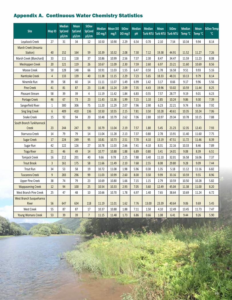
Site Map IDMedian SpCond µS/cm

Mean SpCondµS/cm

StDev SpCond µS/cm

Median DO mg/l

Mean DO mg/l

StDev DO mg/l

Median pH

Median Turb NTU

Mean Turb NTU

StDev Turb NTU

Median Temp °C

Mean Temp °C

StDev Temp °C

Loyalsock Creek 27 31 34 12 10.50 10.90 2.29 6.54 0.70 2.10 7.54 10.34 9.94 8.14Marsh Creek (Ansonia

Station) 40 152 164 59 10.39 10.32 2.08 7.30 7.12 19.38 44.91 11.52 11.27 7.26Marsh Creek (Blanchard) 33 111 118 37 10.86 10.99 2.56 7.37 2.30 8.47 34.47 11.59 11.23 8.08

Meshoppen Creek 20 121 119 26 10.67 11.09 2.30 7.59 2.60 6.97 23.21 11.60 10.69 8.56Moose Creek 50 128 148 66 10.91 11.03 1.55 6.47 0.50 1.78 16.58 9.51 9.93 5.16

Nanticoke Creek 4 133 139 40 11.38 11.15 2.29 7.23 5.65 18.33 48.31 10.13 9.79 8.14Ninemile Run 39 58 60 14 11.11 11.07 1.49 6.99 1.42 3.17 8.66 9.17 9.96 5.56

Pine Creek 41 81 87 23 11.48 11.24 2.09 7.35 4.43 19.96 53.02 10.59 11.44 8.25Pleasant Stream 58 39 39 4 11.19 11.42 1.84 6.83 0.55 7.57 28.77 9.19 9.01 6.23Portage Creek 46 67 73 23 11.43 11.36 1.99 7.15 1.10 2.85 10.24 9.86 9.30 7.39

Sangerfield River 1 300 306 75 11.20 11.29 2.07 7.96 2.90 6.23 22.21 9.74 9.36 7.92Sing Sing Creek 6 409 410 136 10.50 10.55 2.15 7.81 3.50 10.28 40.61 10.35 10.24 7.06

Snake Creek 15 92 94 20 10.48 10.79 2.62 7.06 2.80 10.97 29.34 10.78 10.15 7.88South Branch Tunkhannock

Creek 23 244 247 59 10.79 11.04 2.19 7.57 1.80 5.45 21.23 12.35 12.43 7.93Starrucca Creek 14 79 79 14 11.04 11.28 2.13 7.37 0.80 2.78 13.91 11.40 11.60 7.75

Sugar Creek 17 224 249 95 10.81 10.73 2.51 7.70 4.10 13.19 47.51 11.72 11.46 8.39Sugar Run 42 122 126 27 10.78 11.03 2.66 7.41 4.10 8.31 22.16 10.33 8.46 7.89Tioga River 21 46 49 14 10.77 10.88 1.88 6.89 0.80 3.41 14.01 9.08 8.39 6.51

Tomjack Creek 16 212 201 40 9.66 9.78 2.25 7.88 3.40 11.10 32.01 16.58 16.06 7.37Trout Brook 3 161 175 58 11.66 11.49 2.10 7.68 2.55 8.08 29.80 9.28 9.09 7.44Trout Run 34 53 58 19 10.72 11.08 1.98 5.96 0.30 1.35 5.18 11.12 11.16 6.82

Tuscarora Creek 9 283 296 99 11.03 10.99 2.60 8.00 3.50 9.99 33.16 10.59 9.55 8.96Upper Pine Creek 38 74 79 23 10.69 10.80 1.66 7.15 1.15 2.79 10.59 10.50 10.28 5.82

Wappasening Creek 12 94 100 25 10.54 10.33 2.93 7.05 3.60 12.49 45.04 11.38 11.00 8.20West Branch Pine Creek 25 47 48 10 10.66 10.70 1.78 6.97 1.40 7.65 38.64 10.69 11.24 6.72

West Branch Susquehanna River 56 647 634 118 11.19 11.01 1.62 7.76 13.00 23.39 40.64 9.06 9.69 5.45

West Creek 55 87 87 17 10.37 10.88 1.88 7.11 1.50 4.10 12.49 13.45 11.73 7.47Young Womans Creek 53 39 39 7 11.15 11.48 1.73 6.86 0.66 1.08 6.41 9.44 9.26 5.90

Appendix A. Continuous Water Chemistry Statistics

33

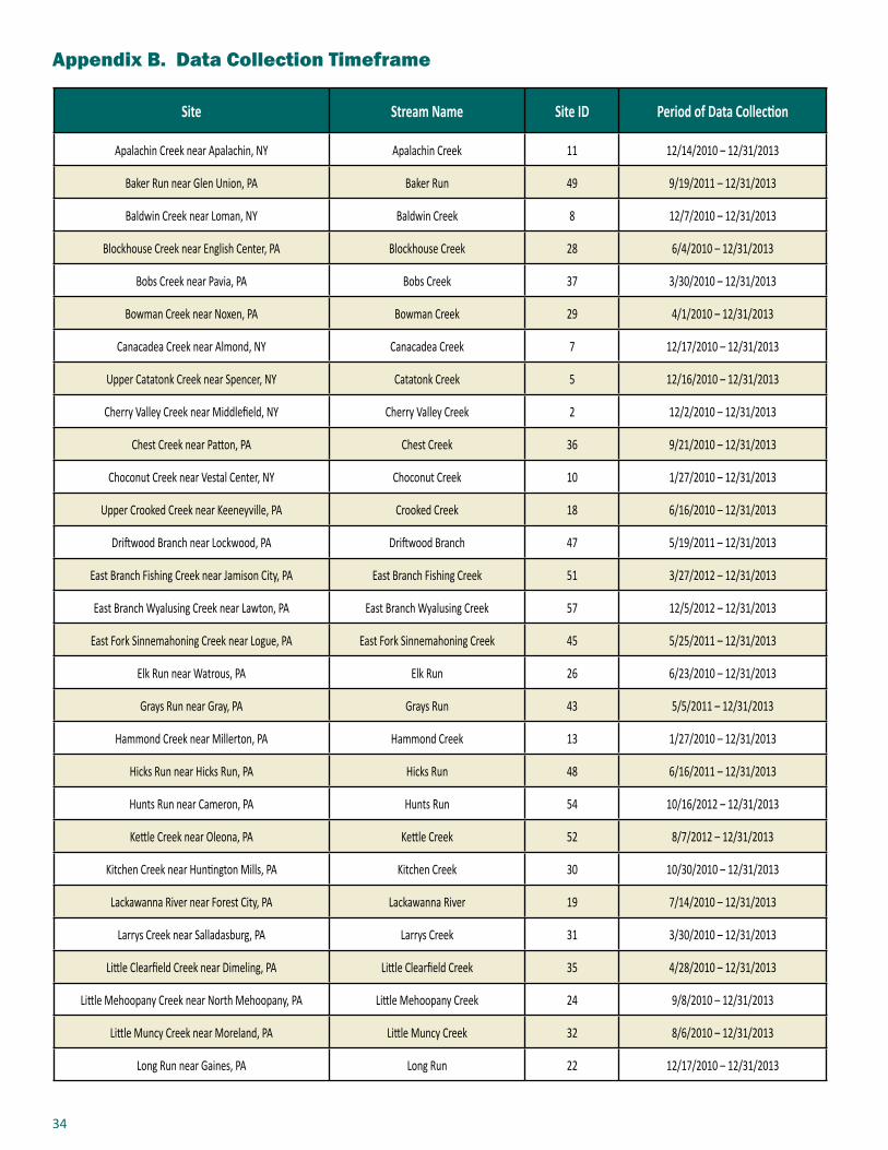
34

Site Stream Name Site ID Period of Data Collection

Apalachin Creek near Apalachin, NY Apalachin Creek 11 12/14/2010 – 12/31/2013

Baker Run near Glen Union, PA Baker Run 49 9/19/2011 – 12/31/2013

Baldwin Creek near Loman, NY Baldwin Creek 8 12/7/2010 – 12/31/2013

Blockhouse Creek near English Center, PA Blockhouse Creek 28 6/4/2010 – 12/31/2013

Bobs Creek near Pavia, PA Bobs Creek 37 3/30/2010 – 12/31/2013

Bowman Creek near Noxen, PA Bowman Creek 29 4/1/2010 – 12/31/2013

Canacadea Creek near Almond, NY Canacadea Creek 7 12/17/2010 – 12/31/2013

Upper Catatonk Creek near Spencer, NY Catatonk Creek 5 12/16/2010 – 12/31/2013

Cherry Valley Creek near Middlefield, NY Cherry Valley Creek 2 12/2/2010 – 12/31/2013

Chest Creek near Patton, PA Chest Creek 36 9/21/2010 – 12/31/2013

Choconut Creek near Vestal Center, NY Choconut Creek 10 1/27/2010 – 12/31/2013

Upper Crooked Creek near Keeneyville, PA Crooked Creek 18 6/16/2010 – 12/31/2013

Driftwood Branch near Lockwood, PA Driftwood Branch 47 5/19/2011 – 12/31/2013

East Branch Fishing Creek near Jamison City, PA East Branch Fishing Creek 51 3/27/2012 – 12/31/2013

East Branch Wyalusing Creek near Lawton, PA East Branch Wyalusing Creek 57 12/5/2012 – 12/31/2013

East Fork Sinnemahoning Creek near Logue, PA East Fork Sinnemahoning Creek 45 5/25/2011 – 12/31/2013

Elk Run near Watrous, PA Elk Run 26 6/23/2010 – 12/31/2013

Grays Run near Gray, PA Grays Run 43 5/5/2011 – 12/31/2013

Hammond Creek near Millerton, PA Hammond Creek 13 1/27/2010 – 12/31/2013

Hicks Run near Hicks Run, PA Hicks Run 48 6/16/2011 – 12/31/2013

Hunts Run near Cameron, PA Hunts Run 54 10/16/2012 – 12/31/2013

Kettle Creek near Oleona, PA Kettle Creek 52 8/7/2012 – 12/31/2013

Kitchen Creek near Huntington Mills, PA Kitchen Creek 30 10/30/2010 – 12/31/2013

Lackawanna River near Forest City, PA Lackawanna River 19 7/14/2010 – 12/31/2013

Larrys Creek near Salladasburg, PA Larrys Creek 31 3/30/2010 – 12/31/2013

Little Clearfield Creek near Dimeling, PA Little Clearfield Creek 35 4/28/2010 – 12/31/2013

Little Mehoopany Creek near North Mehoopany, PA Little Mehoopany Creek 24 9/8/2010 – 12/31/2013

Little Muncy Creek near Moreland, PA Little Muncy Creek 32 8/6/2010 – 12/31/2013

Long Run near Gaines, PA Long Run 22 12/17/2010 – 12/31/2013

Appendix B. Data Collection Timeframe

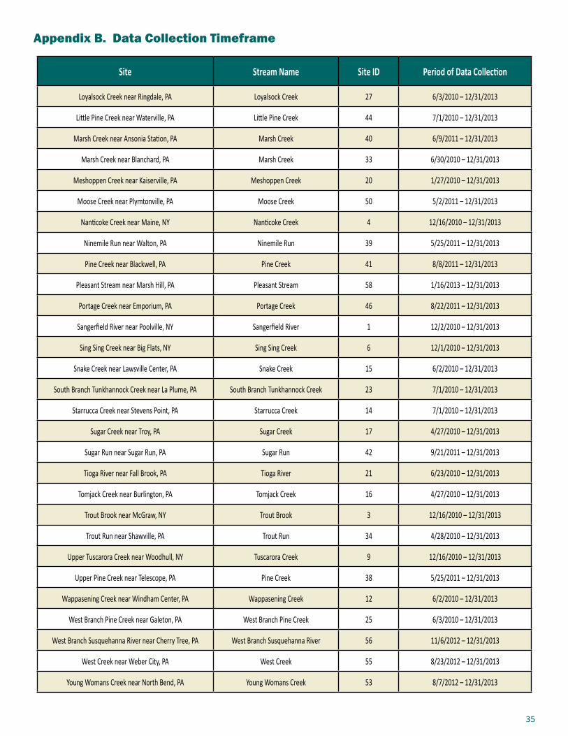
35

Site Stream Name Site ID Period of Data Collection

Loyalsock Creek near Ringdale, PA Loyalsock Creek 27 6/3/2010 – 12/31/2013

Little Pine Creek near Waterville, PA Little Pine Creek 44 7/1/2010 – 12/31/2013

Marsh Creek near Ansonia Station, PA Marsh Creek 40 6/9/2011 – 12/31/2013

Marsh Creek near Blanchard, PA Marsh Creek 33 6/30/2010 – 12/31/2013

Meshoppen Creek near Kaiserville, PA Meshoppen Creek 20 1/27/2010 – 12/31/2013

Moose Creek near Plymtonville, PA Moose Creek 50 5/2/2011 – 12/31/2013

Nanticoke Creek near Maine, NY Nanticoke Creek 4 12/16/2010 – 12/31/2013

Ninemile Run near Walton, PA Ninemile Run 39 5/25/2011 – 12/31/2013

Pine Creek near Blackwell, PA Pine Creek 41 8/8/2011 – 12/31/2013

Pleasant Stream near Marsh Hill, PA Pleasant Stream 58 1/16/2013 – 12/31/2013

Portage Creek near Emporium, PA Portage Creek 46 8/22/2011 – 12/31/2013

Sangerfield River near Poolville, NY Sangerfield River 1 12/2/2010 – 12/31/2013

Sing Sing Creek near Big Flats, NY Sing Sing Creek 6 12/1/2010 – 12/31/2013

Snake Creek near Lawsville Center, PA Snake Creek 15 6/2/2010 – 12/31/2013

South Branch Tunkhannock Creek near La Plume, PA South Branch Tunkhannock Creek 23 7/1/2010 – 12/31/2013

Starrucca Creek near Stevens Point, PA Starrucca Creek 14 7/1/2010 – 12/31/2013

Sugar Creek near Troy, PA Sugar Creek 17 4/27/2010 – 12/31/2013

Sugar Run near Sugar Run, PA Sugar Run 42 9/21/2011 – 12/31/2013

Tioga River near Fall Brook, PA Tioga River 21 6/23/2010 – 12/31/2013

Tomjack Creek near Burlington, PA Tomjack Creek 16 4/27/2010 – 12/31/2013

Trout Brook near McGraw, NY Trout Brook 3 12/16/2010 – 12/31/2013

Trout Run near Shawville, PA Trout Run 34 4/28/2010 – 12/31/2013

Upper Tuscarora Creek near Woodhull, NY Tuscarora Creek 9 12/16/2010 – 12/31/2013

Upper Pine Creek near Telescope, PA Pine Creek 38 5/25/2011 – 12/31/2013

Wappasening Creek near Windham Center, PA Wappasening Creek 12 6/2/2010 – 12/31/2013

West Branch Pine Creek near Galeton, PA West Branch Pine Creek 25 6/3/2010 – 12/31/2013

West Branch Susquehanna River near Cherry Tree, PA West Branch Susquehanna River 56 11/6/2012 – 12/31/2013

West Creek near Weber City, PA West Creek 55 8/23/2012 – 12/31/2013

Young Womans Creek near North Bend, PA Young Womans Creek 53 8/7/2012 – 12/31/2013

Appendix B. Data Collection Timeframe

www.srbc.net

ACKNOWLEDGEMENTS

The Susquehanna River Basin Commission (SRBC) wishes to thank the more than 40 state, county, and local government agencies and private landowners who partnered with SRBC on the installation of the RWQMN stations.

These partnerships made it possible for SRBC to locate and install each monitoring station.

SRBC also thanks the partners who provided the invaluable funding necessary to launch the successful real-time water quality monitoring network. The RWQMN is funded by private and public sector contributions and by SRBC,

which covers the network’s ongoing maintenance expenses. To date, the funding partners are:

East Resources, Inc.New York State Energy Research and Development Authority

Pennsylvania Department of Conservation and Natural ResourcesHeadwaters Resource Conservation & Development Council Sinnemahoning Stakeholders Committee

Chesapeake Energy

West Branch Pine Creek, Potter County, Pa.