12

Renal Regulation of Body Fluids:

Blood volume control

Jeroen van den Akker

BMTE04.35 April 1st 2003

Supervisors: P.M.Bovendeerd (Technical University Eindhoven) I.Groenenberg (Technical University Eindhoven)

mhj

Table of contents

INTRODUCTION........................................................................................................................ 2

1. PHYSIOLOGICAL BACKGROUND ............................................................................... 4

§ 1.1 ANATOMY & PHYSIOLOGY OF THE RENAL FLUID CONTROL SYSTEM............................... 4 § 1.2 TWO PHYSIOLOGICAL CASES OF DISTURBED FLUID BALANCE ......................................... 6

Case I: Iso-osmotic saline infusion .................................................................................... 6 Case II: Pure water loading............................................................................................... 6

2. MODELLING RENAL REGULATION OF BODY FLUIDS ........................................ 7 § 2.1 PRESENTATION OF SCHEMATIC MODEL FOR FLUID REGULATION..................................... 7

2.1.1 Block diagram of the vascular system relevant for controlling body fluid volume... 7 2.1.2 Block diagram of the renal feedback systems for controlling body fluid volume ..... 8

§ 2.2 DESCRIPTION OF MODEL FOR FLUID REGULATION BY IKEDA/MIN ................................ 10 2.2.1 Cardiovascular dynamics........................................................................................ 11 2.2.2 Change in intra-cellular fluid volume..................................................................... 13 2.2.3 Change in interstitial fluid volume.......................................................................... 13 2.2.4 Change in plasma volume ....................................................................................... 14

§ 2.3 DESCRIPTION OF EXISTING MODELS FOR FLUID REGULATION ....................................... 16 2.3.1 Guyton: Circulatory function and cardiac output regulation................................. 16 2.3.2 Dickinson, Ingram & Shephard : Systemic circulation and renal function (MacPee).......................................................................................................................................... 17 2.3.3 Keener & Sneyd: Renal physiology......................................................................... 19 2.3.4 Möller: Renal function and blood pressure stabilization........................................ 22 2.3.5 Moore: Ascending myogenic autoregulation: interactions between tubuloglomerular feedback and myogenic mechanisms................................................... 23

3. SIMULATION RESULTS FOR DISTURBED FLUID BALANCE............................. 28 § 3.1 CASE I: ISO-OSMOTIC SALINE INFUSION ....................................................................... 28 § 3.2 CASE II: PURE WATER LOADING ................................................................................... 31

4. DISCUSSION ..................................................................................................................... 34

§ 4.1 EXPLICATION OF SIMULATION RESULTS........................................................................ 34 § 4.2 COMPARISON OF SIMULATION RESULTS WITH LITERATURE REPORTS............................ 34 § 4.3 RECOMMENDATIONS FOR FUTURE POSSIBILITIES.......................................................... 36

CONCLUSION....................................................................................................................... 37

APPENDIX I: REFERENCES ............................................................................................. 38

APPENDIX II: IMPLEMENTATION OF MODEL FOR FLUID REGULATION BY IKEDA/MIN ........................................................................................................................... 39

APPENDIX III: SYMBOLS AND NORMAL VALUES.................................................... 40

APPENDIX IV: SPECIFICATIONS FOR TWO CASES OF DISTURBED FLUID BALANCE .............................................................................................................................. 44

Case I: Iso-osmotic saline infusion .................................................................................. 44 Case II: Pure water loading............................................................................................. 44

APPENDIX V: LUMPED PARAMETER MODEL........................................................... 45

1

Introduction Proper distribution of fluids throughout the body is critical for human functioning. Extreme fluid retention can result in pulmonary oedema and overstretching of the heart. Also in heart failure, fluid distribution is of critical importance. The human body contains an extensive system for regulating body fluids. Distribution is regulated by the cardiovascular system. The renal system controls the total body water content. Guyton derived a mathematical expression for the calculation of cardiac output (CO) [5]:

( )ss

sssss

CaCvRaRvCaRvCv

aPrPmsCO

+++∗

−= (1)

with: Pms = mean systemic pressure Pra = right atrial pressure Cvs = systemic venous capacitance Rvs = systemic venous resistance Cas = systemic arterial capacitance Ras = systemic arterial resistance Formula 1 clearly illustrates the significance of mean systemic pressure on cardiac output. As can be seen from figure 1, there’s a linear relationship between blood volume and mean systemic pressure. This justifies the need for a model with a detailed description of blood volume regulation, thereby providing a more accurate cardiac output modelling. Such a model could be used to investigate the processes underlying heart failure more thoroughly. Ultimately, new treatment methods can be tested with this model.

Figure 1: Relationship between blood volume and mean systemic pressure [5]

2

This report starts with an explanation on the most relevant physiological processes in regulating blood volume on the intermediate term (~ 1 hour). Chapter two describes a theoretical model containing all elements we defined to be critical in modelling heart failure. This is followed by an already existing model for body fluid control, which is used for implementation. This chapter ends with a description of other models that could be used to extend the implemented model. Chapter three presents the results of simulations in which the fluid balance is disturbed. These results will be discussed in chapter four. The report ends with a conclusion. Appendix V contains a brief description of how to extend the cardiovascular model by T.Arts with a detailed renal function.

3

1. Physiological background

§ 1.1 Anatomy & physiology of the renal fluid control system In this section the role of the kidneys in maintaining a normal body fluids level is discussed. The human body contains other mechanisms for regulating body fluids than the ones explained below, like the phenomenon of vascular stress relaxation. Since we decided to focus on the renal system these won’t be considered here. However, all these processes are determined either mechanically by pressure or volume, or osmotically by concentration. The control of a normal blood volume is closely connected to the body fluids level. This will become more apparent in § 2.2. Anatomy of the kidney Each kidney (see figure 2: left side) is made up of about one million nephrons, the primary operating units (see figure 2: right side). A nephron consists of the glomerulus, through which fluid is filtered from the blood, the juxtaglomerular apparatus, by which glomerular flow is controlled, and the tubule, in which the filtered fluid is converted to urine. The tubule has five sections: the proximal tubule, the descending limb of the loop of Henle, the ascending limb of the loop of Henle, the distal tubule and the collecting duct. The peritubular capillaries reabsorb fluid that has been extracted from the tubules. Blood enters the glomerulus by the afferent arteriole and leaves by the efferent arteriole (see figure 2: right side) [8].

Figure 2: left side: Anatomy of the kidney; right side: Anatomy of the nephron [8] Renal autoregulation Blood is filtered into Bowman’s capsule after passing the glomerular membrane, which is almost completely impermeable to proteins. The glomerular filtration rate is controlled between narrow ranges by way of autoregulation. Renal autoregulation is mediated by two mechanisms: the tubuloglomerular feedback mechanism (TGB) and the myogenic response [11]. Tubuloglomerular feedback mechanism (TGB) TGB is accomplished by the juxtaglomerular complex consisting of macula densa cells in the distal tubule and juxtaglomerular cells in the walls of afferent and efferent arterioles (see figure 3). A low tubular flow rate causes excessive salt-reabsorption in the ascending limb of the loop of Henle resulting in relatively low ionic concentrations at the end of the loop. This results in two regulating mechanisms: the macula densa cells respond by releasing a vasodilator which decreases the resistance of the afferent arterioles and the juxtaglomerular cells release renin which constricts the efferent arterioles by means of a mediator called angiotensin II which is converted out of angiotensin I. The resulting effect of these is an increase in the flow-rate through the glomerulus because the filling

4

pressure of the glomerulus is being elevated. Besides a direct vaso-constricting effect angiotensin II also stimulates the secretion of aldosteron by the adrenal glands. This increases the reabsorption of Na+ ions and, eventually by osmosis, water. This is called the Renin Angiotensin Aldosteron System (RAAS) [1, 4, 8, 13]. Aldosteron secretion can also be stimulated as a result of decreased sodium and potassium concentrations [1].

Figure 3: Structure of the juxtaglomerular apparatus [4] Myogenic response The myogenic response is simply the intrinsic myogenic property of vascular smooth muscle to contract when transmural or intra-vascular pressure rises. This property appears to be act maximally in the preglomerular vasculature [11]. ANF/BNP Besides the pressure-based mechanisms (TGB and myogenic response) there are also some volume-based regulating mechanisms. Specialized granules in the atria release the hormone Atrial Natriuretic Factor (ANF) when being stretched as a result of an increased filling of the heart. ANF diminishes the reabsorption of sodium-ions and inhibits the RAAS system. Similar granules in the ventricles release the hormone Brain Natriuretic Peptide (BNP) in response to stretching. Although contradicting results have been reported, BNP is sure to elevate distal sodium excretion while renal blood flow remains unaffected [7, 9, 14]. In both cases the resulting effect is an increase in water excretion. Reabsorption and excretion of water and sodium The proximal tubule extracts much of the water and dissolved chemicals to be reabsorbed into the bloodstream and concentrates the waste products of metabolism. This reabsorption, up to 65 percent of the glomerular filtrate, takes place by three mechanisms:

• much of the reabsorption occurs by active (co) transport mediated by a Na+/K+-pump • transporters that use the gradient of Na+ ions • watertransport mediated by osmotic pressure

The descending limb of the loop of Henle is highly permeable to water and moderately permeable to ions. The ascending limb plays a major role in the active transport of Na+ from the tubular lumen into the interstitial fluid. This triggers the outflow of water from the descending limb by osmosis, a large portion of the Na+ ions re-enters the descending limb and is reused in this cycle, thus forming a positive feedback mechanism. The proceedings of the ascending section form the juxtaglomerular apparatus where, as mentioned earlier, autoregulation takes place. Passing beyond this point, the distal

5

tubule is reached which has a function similar to the ascending limb. The flow from several nephrons is gathered in the collecting duct and then passes to the bladder [1, 4, 8, 13]. Anti Diuretic Hormone (ADH) The cells lining the collecting duct are sensitive to a number of hormones of which aldosteron and antidiuretic hormone (ADH) are the most important. Aldosteron determines, as mentioned before, the rate at which Na+ ions are transported out of the lumen. ADH, also called vasopressin, increases the permeability of the distal tubules and the collecting duct to water. The ADH level rises in response to increased osmotic pressure [4].

§ 1.2 Two physiological cases of disturbed fluid balance In this section the physiology, as described in § 1.1, will be explained for a number of concrete cases. In chapter 3 these same cases will be checked by a simulation model. Case I: Iso-osmotic saline infusion An increases in fluid intake which is accompanied with sodium intake above the level of urine output causes a temporary fluid accumulation. This results in increased blood volume and extra-cellular volume. The increase in blood volume raises mean circulatory filling pressure and consequently the venous return. Thereby cardiac output and thus arterial pressure are elevated. Urine output is now increased by means of pressure diuresis [4: p.369]. As the cardiac output is increased the blood flow in all the tissues of the body is naturally increased. These vessels constrict by a myogenic response, thus increasing the total peripheral resistance. This resistance increase plays a major role in the elevation of the arterial pressure, which is equal to the product of cardiac output times total peripheral resistance. For instance, despite an increase in cardiac output of only 5 to 10 per cent, a rise in pressure of 100 mm Hg up to 150 mm Hg is not uncommon [4: p.224]. The net effect of this elevated cardiac output and myogenic response is a further increase in arterial pressure. Thus autoregulation returns the blood flow, and thereby the oxygen supply, to a normal level. The raise in cardiac output initiates an increase in the blood flow through the glomerulus. This is counteracted by means of renal autoregulation: the amount of excreted vasoconstrictor is elevated thus increasing the resistance of the afferent arterioles while the excretion of renin is diminished, thereby relaxing the efferent arterioles as a result of a decreased angiotensin level. The simultaneous effect of these is to bring the flow of filtrate through the glomerulus back to the initial level. The decrease in renin concentration also diminishes the activity of the renin angiotensin aldosteron system. ANF, inhibiting sodium reabsorption, is released as a result of the stretched left atrium. Similarly the release of BNP, stimulating sodium excretion, increases by ventricle stretch (see § 1.1). Eventually, fluid excretion is increased until the body fluids have reached their normal values again. Case II: Pure water loading If pure water without any salts is infused the same regulatory mechanisms as described above react. However since fluid becomes more diluted, there will be an additional increase in sodium reabsorption by the Renin Angiotensin Aldosteron System, which is even more active now. Furthermore, fluid excretion will increase since secretion of ADH is suppressed as a result of decreased plasma osmolality [4]. Eventually, body fluid volumes return to normal again.

6

2. Modelling renal regulation of body fluids

§ 2.1 Presentation of schematic model for fluid regulation The total extra-cellular fluid volume is mainly determined by the balance between intake and output of water and salt. These are also the leading determinants for the amount of blood circulating in the vascular system. Although the influence of the salt concentration in the body fluids is certainly not underestimated we choose to neglect it for the time being. The implementation of this aspect would complicate the model enormously since the body contains many compartments for the storage of sodium ions and furthermore many other processes use sodium as well. Of course this has the consequence that in this model, which is designed for studying heart failure, fluid excretion is only determined by pressure diuresis. Pressure natriuresis is neglected. However, the effects of sodium-based hormones are taken into account. 2.1.1 Block diagram of the vascular system relevant for controlling body fluid volume Figure 4 shows a simplified representation of the vascular system relevant for controlling the blood volume. The cardiovascular system consists of one atrium and one ventricle, an arterial compartment and a venous compartment. The pulmonary circulation is neglected here since it has a limited effect in this control system. For instance, the excretion of fluid by the lungs usually not exceeds 20 % of the total amount of fluid-loss by the human body. The amount of body fluids can be adjusted via fluid administration in the interstitial compartment and fluid excretion by the kidneys. Peripheral resistance is determined by the myogenic response based on arterial pressure. Finally, solid lines indicate fluid flows. The thickness of these lines gives a rough indication of the flow magnitude through this tube. The direction of an arrow naturally indicates the flow direction; a double arrow means that the flow direction depends on the conditions determining the equilibrium equation. Dashed lines, which will be used in figure 5, represent all different kinds of mediators like hormones.

Heart (LA) Heart (LV) Arterial compartment

Venous compartment

Interstitial compartment

Intake of fluid

Kidneys

Bladder Excretion of fluid

Peripheral resistance

Figure 4: Basic renal-body fluid feedback mechanism for control of blood volume

7

2.1.2 Block diagram of the renal feedback systems for controlling body fluid volume Now the kidneys are subdivided in their three basic units designed for specific physiological functions: glomerulus, juxtaglomerular apparatus and tubule. As described in § 1.1, the glomerulus forms the primary filter for urine, the juxtaglomerular apparatus controls the amount of produced urine by means of autoregulation and the tubular system regulates the amount of water being reabsorbed. Autoregulation is accomplished by changing the excreted amount of vasodilator, which regulates the diameter of the afferent arterioles, and the amount of renin, which regulates the diameter of the efferent arterioles by means of a mediator called angiotensine. Renin also initiates the activation of the Renin Angiotensin Aldosteron System (RAAS), which stimulates the tubular reabsorption of fluid. The effect of the RAAS is refined by Atrial Natriuretic Factor (ANF), a hormone released when the atria become stretched, which diminishes the reabsorption of sodium ions. A similar system acts in the ventricles: Brain Natriuretic Peptide (BNP), released in response to ventricular stretch, stimulates the excretion of sodium ions. In both cases, the movement of ions builds an osmotic gradient resulting in an accompanying water movement. The effect of BNP on fluid excretion is inhibited by Anti-Diuretic Hormone (ADH), which stimulates water reabsorption (see figure 5).

8

Heart (LA) Heart (LV) Arterial compartment

Venous compartment

Interstitial compartment

Intake of fluid

P

+ Decrease Afferent

Figure 5: Extended renal-body fluid feedba

ANF

Vasodilator/ -constrictor

+

Resistance

BN

Peripheral re

Water Reabsorption

+ Sodium Excretion

Juxtaglom. apparatus

Glomerulus

Autoregulation

Bladder

+

Renin/ Angiotensin

RAAS

+

+Increase Efferent Resistance

+

+

+

-

-Sodium

Reabsorption

Tubule

ck mechanism

9

Excretionof fluid

sistan

for co

ADH

ce

ntrol of blood volume

§ 2.2 Description of model for fluid regulation by Ikeda/Min After the development of a theoretical model for body fluid regulation containing the essential elements, as defined in chapter § 2.1, we had to choose an existing model for further investigation. The model used for implementation, FLUIDS, was developed by Min [1982,1993], who used a model designed by Ikeda [1979] based on work of Guyton [1972] and Blaine [1972]. This choice was based partially on the good criticism this model had received in various literature reports. Just like the model by Dickinson (MacPee), it contains a detailed description of renal functioning in combination with a basal blood circulation. However, despite the abundant documentation on MacPee, there’s no complete source code available, as is the case for Ikeda/Min. The Ikeda/Min model consists of several sub-systems: circulation, respiration, renal function and the intra- and extra-cellular fluid compartments. The renal function is subdivided into three compartments: metabolic acid-base balance, urine excretion and controller of renal function (see figure 6). In this type of model not only the body fluids can be studied, but also acid-base disorders can be investigated. The parameter values used are average values found in literature for a healthy human male of approximately 55 kg.

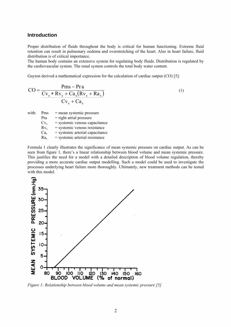
Figure 6: General overview of the model by Min: FLUIDS [15] Now each compartment, as defined in figure 6, will be transformed to a block with specific constants, inputs and outputs (figure 7). Ikeda provided a detailed description of each block [6]. However, after an introduction on cardiovascular dynamics, we will focus on the fluid compartments. The body fluids are divided into three groups (see figure 8): intracellular fluids (VIC = 20,0 litre), interstitial fluids (VIF = 8,8 litre) and plasma (VP = 2,2 litre). Trans-cellular water (brain fluid, eye fluid etc.) is ignored since this amount is relatively small. This accounts for a total fluid content of 20,0 + 8,8 + 2,2 = 31 litre. The regulation of blood volume is of special interest, since this is the major determinant of cardiac output, see formula 2 [5].

10

Figure 7: Fluid and electrolyte regulation by Ikeda [6], with some modifications: Block 3: left side: PVC replaced by PVS Block 4: right side: VIC added Block 5: left side: YNE replaced by XNE Block 7: left side: YNH, VIC added 2.2.1 Cardiovascular dynamics The cardiovascular unit (block 1) has been minimized since it is only used to supply a blood circulation for the investigation of the regulation of body fluids. Such a simplified structure has the advantage that steady state values are reached much easier since short-term processes as auto regulation and stress relaxation are being neglected. Stress relaxation is the phenomenon that vessels become stretched in response to an elevated pressure, thereby gradually reducing this pressure to it’s normal level [4: 235]. As a result of these simplifications, this model had as limited use for the investigation of cardiovascular problems. In the real heart, according to the Frank-Starling mechanism, which is valid in a normal physiological range, the cardiac output increases with an increased filling of the ventricles [12]. This filling depends on the venous pressure, which in turn depends on the blood volume. In the underlying model, cardiac output (QCO: litre/min) is a direct function of the blood volume (VB: litre):

0QCOVBaQCO +∗= (2) with: a = 1,0 (min)-1

QCO0 = 1,0 litre/min

11

Mean arterial pressure (PAS: mmHg) is assumed to be a function of cardiac output and peripheral resistance (RTOT: mmHg*min/litre):

0* PASRTOTQCOPAS += (3) with: PAS0 = 20 mmHg Thus blood volume determines arterial pressure directly via cardiac output. For the pressures in systemic veins and pulmonary circulation a similar linear approximation of the Frank-Starling mechanism is taken.

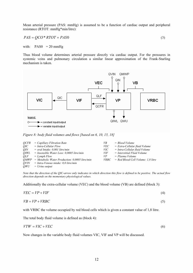
Figure 8: body fluid volumes and flows [based on 6, 10, 15, 18] QCFR = Capillary Filtration Rate VB = Blood Volume QIC = Intra-Cellular Flow VEC = Extra-Cellular fluid Volume QIN = oral Intake: 0,001 litre/min VIC = Intra-Cellular fluid Volume QIWL = Insensible Water Loss: 0,0005 litre/min VIF = Interstitial Fluid Volume QLF = Lymph Flow VP = Plasma Volume QMWP = Metabolic Water Production: 0,0005 litre/min VRBC = Red Blood Cell Volume: 1,8 litre QVIN = Intra-Venous intake: 0,0 litre/min QWU = Urine output Note that the direction of the QIC-arrow only indicates in which direction this flow is defined to be positive. The actual flow direction depends on the momentary physiological values. Additionally the extra-cellular volume (VEC) and the blood volume (VB) are defined (block 3):

VIFVPVEC += (4)

VRBCVPVB += (5) with VRBC the volume occupied by red blood cells which is given a constant value of 1,8 litre. The total body fluid volume is defined as (block 4):

VECVICVTW += (6) Now changes in the variable body fluid volumes VIC, VIF and VP will be discussed.

12

2.2.2 Change in intra-cellular fluid volume The intra-cellular volume is a function of the intra-cellular flow, which is dependant on various ion concentrations (block 3):

( ) QICdtVICd

= (7)

QIC is the rate of water flow into intracellular space driven by an osmotic gradient (block 4):

( CSMXGLEXKEXNEXKIQIC 5,10 )+−−−= (8) with: XKI = ICF potassium concentration (mEq/litre) XNE = ECF sodium concentration (mEq/litre) XKE = ECF potassium concentration (mEq/litre) XGLE = ECF glucose concentration (mEq/litre)

CSM = transfer coefficient of water from ECF to ICF caused by this osmotic gradient ICF = Intra-cellular fluid ECF = Extra-cellular fluid

Calculation of the concentrations (X: mEq/litre) of these substances is very straightforward:

VZsXs = (9)

with: s = one of the ions mentioned above Z = content (mEq) V = intra-/extra-cellular volume (litre) Changes in these contents are calculated as follows (block 4):

( ) YsUYsIdtZsd

−= (10)

with: Y = flow (mEq/min)

I = intake (litre/min) U = excretion (litre/min)

These excretions are all dependant on, among others, the glomerular filtration rate (GFR, see § 2.2.4). This is described in detail by Ikeda [6]. 2.2.3 Change in interstitial fluid volume The interstitial fluid volume (VIF) may change due to the outflow from capillaries (QCFR), the lymphatic outflow (QLF) and the flow into/out of the intracellular space (QIC):

( ) QICQLFQCFRdtVIFd

−−= (11)

QLF is an exponential function of interstitial fluid pressure (PIF) derived from Guyton (block 3). QIC depends on the osmotic gradient, as described previously (block 4). QCFR equals the product of a capillary filtration coefficient (CFC) and the filtration pressure (PF) (block 3):

13

CFCPFQCFR ∗= (12) The capillary filtration coefficient, CFC, is set to 0,007 litre/min/mm Hg while for the filtration pressure holds:

PICOPPCOPIFPCPF +−−= (13) with: PC = capillary pressure, dependant on systemic arterial & venous pressure PIF = interstitial fluid pressure, dependant on VIF

PPCO = plasma colloid osmotic pressure PICO = interstitial colloid osmotic pressure 2.2.4 Change in plasma volume The plasma volume (VP) is determined by:

( ) QWUQCFRQIWLQLFQMWPQVINQINdtVPd

−−−+++= (14)

with: QIN = prescribed oral intake

QVIN = prescribed intravenous injection QMWP = prescribed metabolic water production QLF = lymphatic flow, assumed to be an exponential function of interstitial fluid

pressure (PIF) derived from Guyton, as described previously (block 3) QIWL = prescribed insensible water loss (e.g. sweating) QCFR = capillary filtration rate, assumed to be the product of a capillary filtration

coefficient (CFC) and the filtration pressure (PF), as described previously (block 3)

QWU = urine output (block 6) The quantity of water administered orally (QIN) is a function of the oral water intake (VIN). Once this this water administration has started, 10 % of the original value of VIN will be shifted into the plasma volume for each time step. In each next time step, 10 % of the remaining value of VIN will be added to VP (block 3). The regulation of urine output (QWU), which is one of the major determinants of blood volume, is the most complex part of this model:

( ADHQWDQWU 9,00,1 −= ) (15) with ADH the excreted Anti Diuretic Hormone. Thus, since ADH has a normalized value of one, the total fluid reabsorption is 90 % in equilibrium. For the rate of urinary excretion in the distal tubule (QWD) the following function is assumed:

[ ]( ) OSMPYMNUYURUYGLUYKDYNDQWD /32,086,1 +++++= (16) with: YND = rate of sodium excretion in distal tubule (litre/min) YKD = rate of potassium excretion in distal tubule (litre/min) YGLU = renal excretion rate of glucose (litre/min) YURU = renal excretion rate of urea (litre/min) YMNU = renal excretion rate of mannitol (litre/min) OSMP = plasma osmolality (mOsm/litre)

14

This equation is valid since the reabsorption of water is assumed to be iso-osmotic down the distal tubule. Plasma osmolality is a function of the concentration (X) of all osmotic active ions in the extra-cellular (E) fluid compartment (block 4):

( ) 73,986,1 +++++∗= XMNEXUREXGLEXKEXNEOSMP (17) The formula for distal tubule urinary excretion is one of the most important elements of this model and therefore needs further explanation. The renal excretion rates of glucose (YGLU), urea (YURU) and mannitol (YMNU) all depend directly on the glomerular filtration rate (block 4). The glomerular filtration rate (GFR: litre/min) represents the pressure-based auto regulation coordinated by a volume receptor, VEC (block 7):

0,11/10 VECGFRGFRGFR ∗∗= (18) with GFR0 the normal value of GFR and GFR1 a function dependant on the magnitude of the mean arterial pressure (PAS). However it should be noticed that GFR1 itself is just a mathematical function, not representing any physiological process. Therefore two different versions of GFR1 coexist (block 6 & 7), as will be seen later on. The rate of potassium excretion in the distal tubule is given by (block 6):

( ) ( ALDXKEcGFRXKEcYKD )∗∗+∗∗= 21 1 (19) with: c1, c2 = constants (mEq/min) ALD = amount of aldosteron released, compared to normal

THDFCPRXGFRGFR ∗∗=1 (20) with: CPRX = excretion ratio of filtered load after the proximal tubule (0,2)

THDF = complementary control factor, which will be explained later The rate of sodium excretion in the distal tubule is given by (block 6):

( ) ( ALDYNHYND ∗−∗= 09,09,0 ) (21) with YNH the rate of sodium excretion in Henle’s loop, for which holds:

15,0 GFRXNEYNH ∗∗= (22) with GFR1 and CPRX as defined for YKD

ADH is dependent on the pulmonary venous pressure (PVP) and plasma osmolality, representing volume receptors and osmoreceptors (block 7). The secretion of aldosteron, mediated by the renin-angiotensin system, is assumed to be dependant on the ECF potassium concentration, the rate of sodium excretion in Henle’s loop, PVP and PAS [6]. The role of aldosteron in these processes is the stimulation of the reabsorption of sodium and excretion of potassium in the distal tubule, as can been seen directly from formulas 19 and 21. Since the aldosteron system takes some time to react, a buffer system is build in which delays the reaction with a period of 100 minutes (block 7). THDF has been added to refine the effect of body fluid volume expansion on increased urinary output, already taken partially into account by ADH and aldosteron. THDF increases with an increasing plasma colloid osmotic pressure but cannot reach a value lower than it’s normal value (block 7) [6, 10, 15, 18].

15

§ 2.3 Description of existing models for fluid regulation Besides the Ikeda/Min model, several models for the regulation of body fluids have been proposed. The goal of this section is not to give a complete overview of these models, but merely to introduce the most widely used concepts in this field of investigation, with a focus on the main characteristics of each model. Also an attempt will be made to explain how these models differ from the Ikeda/Min model and how they can be of additional value by combining them with the implemented model. 2.3.1 Guyton: Circulatory function and cardiac output regulation The model Guyton developed is a very complex analysis of circulatory function and cardiac output regulation (see figure 9). It contains compartments for circulatory dynamics, heart rate and stroke volume, autonomic control, non-muscle local blood flow control, non-muscle oxygen delivery, muscle blood flow control and PO2, vascular stress relaxation, pulmonary dynamics and fluids, red blood cells and viscosity, heart hypertrophy or deterioration, capillary membrane dynamics, kidney dynamics and excretion, tissue fluids, pressures and gel, thirst and drinking, electrolytes and cell water, antidiuretic hormone control, angiotensin control, and aldosteron control [5].

Figure 9: Circulatory function and cardiac output regulation [5] Although this model is extremely extensive, the renal function is relatively simple [6]. However, this model is widely used as the basis for many models of body fluid regulation [6, 10, 15]. Especially the compartments describing circulatory function could be used to refine the simple cardiovascular dynamics model by Ikeda/Min.

16

2.3.2 Dickinson, Ingram & Shephard : Systemic circulation and renal function (MacPee) Macpee studies the long-term interaction between circulation, kidneys, body fluids and electrolytes. General body autoregulation and systemic arterial baroreceptor reflex have also been taken into account. The model can therefore be used to study the adaptations which take place when changes in body fluids and electrolytes occur, or to study the effects of changes in haemodynamic function on body fluids. In the procedure used in this model, redistribution of water and electrolytes is computed with a time step of typically 60 minutes in accordance with concentration gradients and osmotic pressures. All variables are based on a healthy, young, 70 kg man

Figure 10: Overview of possibilities in MacPee [17] Figure 10 shows a general outline of the main elements in this model. The most important components, systemic circulation and renal function, will be discussed briefly now. In the systemic circulation, the arterial pressure is a direct function of extra-cellular sodium and angiotensin. The extra-cellular sodium quantity is the difference between dietary sodium intake minus urinary sodium loss, the plasma angiotensin concentration is proportional to the plasma renin activity. This activity depends on the renin secretion minus the renin degradation, while the secretion, as well as the synthesis, of renin are controlled by the macula densa feedback signal (see figure 11). However there is no explicit definition of the volume compartments and the flows in and out of these compartments like in Ikeda/Min (see figure 8).

17

Figure 11: Systemic circulation and renal function [based on 17] The kidney consists of an afferent artery, a glomerulus, an efferent artery, a proximal tubule, a distal tubule and a collecting duct. The vascular conductance in the afferent artery is determined by the macula densa feedback signal (-) and the myogenic response (-). This feedback signal depends on the macula densa sodium flow and the angiotensin concentration (picogram/millilitre) while the myogenic response simply states that an increasing pressure causes vasoconstriction. In this case the conductance decreases with increasing arterial pressure (AP: mmHg). For the vascular conductance in the efferent artery a function of the macula densa feedback signal and angiotensin concentration is assumed. The glomerular filtration rate (GFR: millilitre/min) is the product of the net pressure gradient across the glomerular membrane (NetP: mmHg) and a membrane filtration coefficient, with NetP as follows:

AveCOPPTPGPNetP −−= (23) with: GP = Glomerular Pressure (mmHg) PTP = Proximal Tubule Pressure (mmHg) AveCOP = Average Colloid Osmotic Pressure (mmHg) The colloid osmotic pressure is a quadratic function of plasma protein concentration, which itself depends on the filtration fraction, defined as the quotient of GFR and renal plasma flow (RPF: millilitre/min):

( HctRBFRPF −∗= 0,1 ) (24) with Hct (-) the hematocrit and RBF (millilitre/min), the renal blood flow, defined as follows:

18

( ) ⎟⎟⎠

⎞⎜⎜⎝

⎛++∗−=

VenCEffCAffCVPRAPRBF 111/1 (25)

with: RAP = Renal Artery Pressure (mmHg) VP = Venous Pressure (mmHg)

AffC = Afferent Conductance (millilitre/min/mmHg) EffC = Efferent Conductance (millilitre/min/mmHg) VenC = Venous Conductance (millilitre/min/mmHg) Note that renal artery pressure is normally equal to arterial pressure in this model. The proximal tubule sodium reabsorption is influenced by the sodium load and angiotensin concentration. The release of angiotensin also initiates the production of aldosteron, with a time delay of 240 minutes. Aldosteron then stimulates the sodium reabsorption in the distal tubule. Finally, dependant only on the sodium concentration, more sodium is reabsorbed in the collecting duct [3, 10, 16, 17]. In comparison with the model by Ikeda/Min, renal haemodynamics are extended here with a bloodstream in and out of the kidneys. Furthermore it can be noticed that the macula densa feedback signal and the role of angiotensin is dealt with quite extensively. However, Anti Diuretic hormone has not been taken into account. Especially the implementation of afferent and efferent arteries, regulated by the macula densa feedback mechanism, looks promising. 2.3.3 Keener & Sneyd: Renal physiology This model focuses on the process by which urine is formed and waste products are removed from the bloodstream. Several mechanisms occurring in the kidneys are discussed separately, according to the anatomical positions where these processes take place. The glomerulus forms the primary filter. Three pressures affect the rate of glomerular filtration:

• pressure in glomerular capillaries (promotes filtration): P1 (“60 mm Hg”) • pressure in Bowman’s capsule (opposes filtration): P2 (“18 mm Hg”) • colloidal osmotic pressure of plasma proteins inside capillaries (opposes filtration): лc

Now assume that the glomerular capillaries and the surrounding Bowman’s capsule both comprise a one-dimensional tube (see figure 12). For the rate of change of the flow in the capillary follows:

( ) RTc,PPKdxdq

cc12f1 =ππ+−= (26)

with: Kf = capillary filtration rate

c = concentration varying with x since the suspension becomes more concentrated as it moves through the glomerulus.

Figure 12: model of glomerulus [8]

19

Furthermore for the flow out of the afferent arteriole into the glomerulus (qi), the flow out of the glomerulus into the efferent arteriole (qe) and the flow out of the glomerulus into the proximal tubule, which in this case equals the descending tubule (qd), is assumed respectively:

( )a

ai R

PPq 1−

= (27)

( )

e

ee R

PPq

−= 1 (28)

( ) ( )d

deid R

PPqqq

−=−= 2 (29)

with: Pa = pressure in afferent arteriole (“100 mm Hg”) Ra = resistance of afferent arteriole Pe = pressure in efferent arteriole (“18 mm Hg”) Re = resistance of efferent arteriole Pd = pressure in descending tubule (“14-18 mm Hg”) Rd = resistance of descending tubule Renal autoregulation depends on the activity of vasodilators and vasoconstrictors. A simple model to simulate this is to make the arteriole resistances dependant on the rate of filtration:

(([ tdaaa qqrR −+= ))]δtanh1 (30)

(([ tdeee qqrR −+= ))]δtanh1 (31) with: qt = target flow rate (“125 ml/min”)

ra = normal resistance-value re = normal resistance-value δa = sensitivity of the model to changes in flow rate (“δa = 0,1”) δe = sensitivity of the model to changes in flow rate (“δe = 0,01”)

This section could be used to complete the Ikeda/Min model with a detailed description of renal autoregulation, once afferent and efferent arteries have been defined. The next step is the modelling of the loop of Henle. This is done by a partition into four compartments: descending limb (“.d”), ascending limb (“.a”), collecting duct (“.c) and a combined compartment for interstitium and peritubular capillaries (“.s”). The last compartment accepts fluids from the three tubules and loses it to the venules (see figure 13). The only ion considered is sodium, since this concentration determines 90 % of the osmotic pressure. Differences in sodium transport properties along the tubules however are being ignored in this model.

20

Figure 13: model of Henle’s loop [8] Now the flow of water and Na+ ions out of their compartments can be deduced for the descending limb, ascending limb and collecting duct respectively:

( sddssd

d

ccRTPPdx

dqk

−+−−=∗ 21 π ) (32)

with kd the permeability of the descending limb to water

( ) ( dsddd cch

dxcqd

−=∗ ) (33)

with hd the permeability of the descending limb to sodium ions

0=dx

dqa (34)

( )

pdx

cqd aa −=∗

(35)

with p a constant pump rate

( sccssc

c

ccRTPPdxdq

k−+−−=∗ 21 π ) (36)

with kd the permeability of the collecting duct to water

( ) ( csccc cch

dxcqd

−=∗ ) (37)

with hd the permeability of the collecting duct to sodium ions Note that the sodium transport in the ascending limb isn’t governed by simple diffusion but by an active process and that this tubule is impermeable to water.

21

Fluid conservation gives the equations for the peritubular capillaries:

( )dx

qqqddxdq cads ++

−= (38)

( ) ( )

dxcqcqcqd

dxcqd ccaaddss ∗+∗+∗

−= (39)

Finally, this set of equations is completed by four equations of the form:

jjj qR

dxdP

∗−= (40)

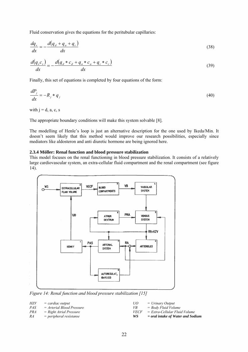
with j = d, a, c, s The appropriate boundary conditions will make this system solvable [8]. The modelling of Henle’s loop is just an alternative description for the one used by Ikeda/Min. It doesn’t seem likely that this method would improve our research possibilities, especially since mediators like aldosteron and anti diuretic hormone are being ignored here. 2.3.4 Möller: Renal function and blood pressure stabilization This model focuses on the renal functioning in blood pressure stabilization. It consists of a relatively large cardiovascular system, an extra-cellular fluid compartment and the renal compartment (see figure 14).

Figure 14: Renal function and blood pressure stabilization [15] HZV = cardiac output UO = Urinary Output PAS = Arterial Blood Pressure VB = Body Fluid Volume PRA = Right Atrial Pressure VECF = Extra-Cellular Fluid Volume RA = peripheral resístanse WS = oral intake of Water and Sodium

22

The blood pressure is controlled by the urinary output: UO = a12*PAS2 + a11*PAS + a10 (41) The extra-cellular fluid volume is assumed as follows:

( ) UOWSdt

VECFd−= (42)

For the body fluid volume the following function is used: VB = a22*VECF2 + a21*VECF + a20 (43) This controls then the mean systemic pressure (PMS): PMS = a32*VB2 + a31*VB + a30 (44) with aij various constants Urinary output (UO) increases with an elevated arterial pressure (PAS). This causes a decrease in the body fluid volume (VB) and concurrently in the mean systemic filling pressure (PMS). Then venous return (VR) decreases, as does right atrial pressure (PRA). Ultimately this results in a decreased cardiac output (Frank-Starling law) [15]. This relatively simple model could be used to check the urinary output produced in Ikeda/Min as a result of a certain increased arterial pressure. Complex regulating functions have then been replaced by a few simple constants. 2.3.5 Moore: Ascending myogenic autoregulation: interactions between tubuloglomerular feedback and myogenic mechanisms Moore developed a model of the renal vascular and tubular systems to study any possible interactions between the tubuloglomerular feedback mechanism and the myogenic response. The ascending myogenic response (AMYO) was a particular area of interest. The renal vascular system is modelled with six lumped resistances connected in series: the basal resistance of the preglomerular vessels (Rb), the resistance increment contributed by the descending myogenic response (∆Rmd), the resistance increment contributed by the ascending myogenic response (∆Rma), the increment in resistance owing to TGF (∆Rtgf), the resistance of the glomerular capillary bed (Rg) and the resistance of the postglomerular vasculature (Re). The pressure is defined at four points in this system: the systemic arterial pressure (Pas), the pressure at the entrance to the glomerular capillary bed (Pg), the abdominal venous pressure (Pv = 0), and the intra-vascular pressure just upstream from the site of TGF resistance changes (Pn) (see figure 15).

23

Figure 15: Renal micro-vasculature modelled by lumped resistances [11] Now consider two cases, first the case in which TGF is ignored (Pn) followed by the case in which the onset of a TGF response will introduce an additional resistance increment in ∆Rtgf and accordingly in ∆Rma (Pn’). We can write for intra-vascular pressure respectively:

( )( )egmdb

egvasn RRRR

RRPPP

++∆+

+−= (45)

( )( )

tgfmaegmdb

tgfegvasn RRRRRR

RRRPPP

∆+∆+++∆+

∆++−=' (46)

The magnitude of the ascending myogenic response necessary to keep Pn constant can be found by equating the two equations mentioned above, with the following result:

⎟⎟⎠

⎞⎜⎜⎝

⎛

+∆+

∆∗=∆eg

mdbtgfama RR

RRRGR (47)

with Ga a scaling coefficient, for which holds: Ga = 0: no AMYO response

Ga = 1: maximal AMYO response which keeps Pn constant, despite the TGF-mediated vasoconstriction

24

Similarly for the DMYO follows:

( egtgfmabas

asdmd RRRRR

PP

GR ++∆+∆+⎟⎟⎠

⎞⎜⎜⎝

⎛−=∆ 1

0

) (48)

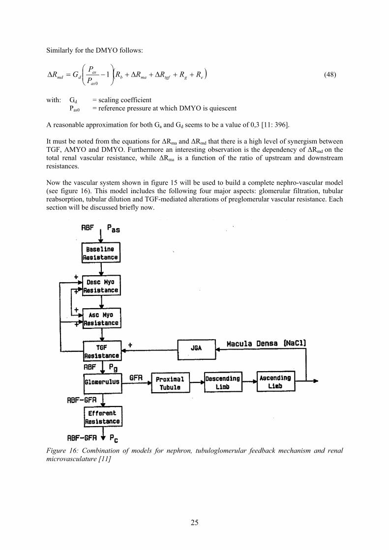
with: Gd = scaling coefficient Pas0 = reference pressure at which DMYO is quiescent A reasonable approximation for both Ga and Gd seems to be a value of 0,3 [11: 396]. It must be noted from the equations for ∆Rma and ∆Rmd that there is a high level of synergism between TGF, AMYO and DMYO. Furthermore an interesting observation is the dependency of ∆Rmd on the total renal vascular resistance, while ∆Rma is a function of the ratio of upstream and downstream resistances. Now the vascular system shown in figure 15 will be used to build a complete nephro-vascular model (see figure 16). This model includes the following four major aspects: glomerular filtration, tubular reabsorption, tubular dilution and TGF-mediated alterations of preglomerular vascular resistance. Each section will be discussed briefly now.

Figure 16: Combination of models for nephron, tubuloglomerular feedback mechanism and renal microvasculature [11]

25

Glomerular filtration The afferent blood flow (Ba) can be calculated as follows:

( )tgfmamdba

a

gasa RRRRR

RPP

B ∆+∆+∆+=−

= , (49)

with Ra the total preglomerular resistance. The nephron filtration rate (G) is expressed as:

ea QQG −= (50) This results in the following efferent blood flow (Be):

GBB ae −= (51) Tubular reabsorption Tubular reabsorption is assumed to occur purely in the proximal tubule and the descending limb of Henle’s loop. The proximal tubule is subdivided anatomically into two sections: a superficial proximal convoluted segment (.lp) and a straight proximal segment (.ep). The tubular flows are calculated as follows:

( ) pplp RFGQ −−= 1 (52)

( ) sslpep RFQQ −−= 1 (53) with: Fp = fractional tubular fluid reabsorption in convoluted segment (0,6) Rp = constant rate of tubular fluid reabsorption in convoluted segment (0) Fs = fractional tubular fluid reabsorption in straight segment (0,1) Rs = constant rate of tubular fluid reabsorption in straight segment (0) Thus, 64 % of the tubular fluid load is reabsorbed in the proximal tubule. As isotonic reabsorption is assumed, the sodium concentration is constant and equal to the cortical interstitial sodium concentration (Cic) at the bend of Henle’s loop. For the descending limb impermeability to sodium and equilibrium between tubular fluid and medullary interstitium (.im) is assumed. Hence, the flow entering the ascending limb of Henle’s loop (Qalh) and its sodium concentration (Calh) are:

⎟⎟⎠

⎞⎜⎜⎝

⎛=

im

icepalh C

CQQ (54)

imalh CC = (55)

with typical values of Cic = 150 mM and Cim = 300 mM. Tubular dilution It is assumed that the flow is constant along the ascending limb of Henle’s loop, since this section is impermeable to water. Thus, only NaCl transport is considered. The ascending limb, with a length of x = 0,6 cm, is subdivided equally into the outer medulla and the cortex. The medulla starts in the bend of the loop, resulting after 0,3 cm in the cortico-medullary boundary. Here starts the cortex, ending at x = 0,6 cm at the macula densa.

26

For the outer medulla conservation of NaCl leads to:

⎟⎟⎠

⎞⎜⎜⎝

⎛−=

alh

alh

QJr

dxdC

π2 (56)

with: Calh = salt concentration r = radius of the ALH (10 µm) J = net flux of NaCl out of the ALH, for which holds:

( ) alhmisalhs CVCCPJ +−= (57) with Ps = NaCl permeability of the ALH Vm = active transport coefficient Cis = interstitial NaCl concentration, defined as follows: Cis = Cim - K1*x where K1 = 50 mM/mm for 0 ≤ x ≤ 0,3 Cis = 150 mM for 0,3 < x ≤ 0,6 The sodium chloride reabsorption in the cortex is calculated by the same conservation equation as was valid for the medulla, with the exceptions that Cis is replaced by Cim and by using the concentration at the cortico-medullary junction as the initial condition. TGF-mediated alterations of preglomerular vascular resistance Schnermann et al. developed an empirical relationship for the TGF-mediated alterations of preglomerular vascular resistance, dependant on the luminal chloride concentration (Ci): ∆Rtgf = 0 for Ci < Ct∆Rtgf = Ktgf*(Ci – Ct) for Ct ≤ Ci ≤ Cs∆Rtgf = Ktgf*(Cs – Ct) for Ci > Cswith: Ct = threshold concentration (25 mM) Cs = saturated concentration (60 mM) Ktgf = coefficient of TGF response curve (0,0043 mm Hg/((nl/min)(mM))) Now the model is complete, as depicted in figure 16, and can be solved by an iterative method [11]. This model contains features also occurring in the models by Dickinson [3, 10, 16, 17] and Keener [8]. Clearly, this description is even more detailed. A disadvantage of the model by Moore seems that many parameters are estimates based on animal experiments. It therefore depends on the demands of future users which of these models is the most suitable one. In combination with the model of Ikeda/Min, the method proposed by Dickinson seems most easy to implement since this description resembles the one used by Ikeda/Min in a high degree.

27

3. Simulation results for disturbed fluid balance In this section the behaviour of the implemented Ikeda/Min model is tested for iso-osmotic infusion and water loading. These two cases were described extensively in § 1.2.

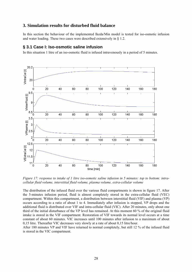
§ 3.1 Case I: Iso-osmotic saline infusion In this situation 1 litre of an iso-osmotic fluid is infused intravenously in a period of 5 minutes.

Figure 17: response to intake of 1 litre iso-osmotic saline infusion in 5 minutes: top to bottom: intra-cellular fluid volume, interstitial fluid volume, plasma volume, extra-cellular volume The distribution of the infused fluid over the various fluid compartments is shown in figure 17. After the 5-minutes infusion period, fluid is almost completely stored in the extra-cellular fluid (VEC) compartment. Within this compartment, a distribution between interstitial fluid (VIF) and plasma (VP) occurs according to a ratio of about 1 to 4. Immediately after infusion is stopped, VP drops and the additional fluid is distributed over VIF and intra-cellular fluid (VIC). After 20 minutes, only about one third of the initial disturbance of the VP level has remained. At this moment 60 % of the original fluid intake is stored in the VIF compartment. Restoration of VIF towards its normal level occurs at a time constant of about 60 minutes. VIC increases until 100 minutes after infusion to a maximum of about 0,15 litre. Thereafter VIC decreases very slowly at a rate of about 0,15 litre/hour. After 180 minutes VP and VIF have returned to normal completely, but still 12 % of the infused fluid is stored in the VIC compartment.

28

Figure 18: response to intake of 1 litre iso-osmotic saline infusion in 5 minutes; top: arterial pressure; bottom: urine output Arterial pressure (PAS) increases rapidly to a maximum of 116,4 mmHg immediately after the infusion period (figure 18: top). This follows directly from the elevated plasma volume (figure 17, formula 3). Within 15 minutes after infusion is stopped, the raise in PAS is brought back with two third to about 105 mmHg. However after 180 minutes the pressure level is still slightly higher than in the original situation. The urinary system needs some time to respond to an elevated plasma level (figure 8). During the first 5 minutes, only 10 millilitre urine is produced additionally in response to 1 litre infused fluid (figure 18: bottom). After 20 minutes a maximal urine output (QWU) of 13,1 millilitre/minute is reached, 13 times as great as in the normal situation. It takes about 100 minutes to reduce QWU to one third of its maximum. After 180 minutes the normal level of 1 millilitre/minute is reached. Clearly, a large portion of the administered fluid is removed as urine (figure 18: bottom). The irregularity after 5 minutes in QWU is probably the result of an error in the program code for visualization but this doesn’t seem to affect the simulation itself.

29

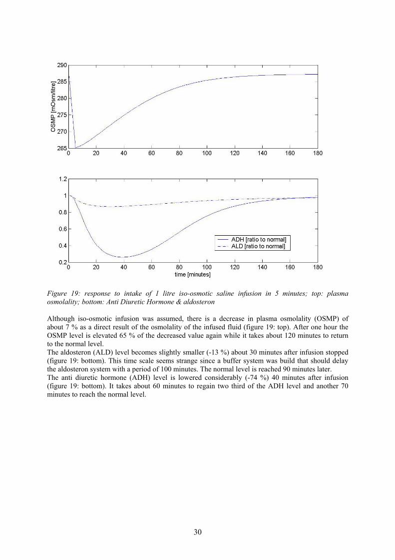
Figure 19: response to intake of 1 litre iso-osmotic saline infusion in 5 minutes; top: plasma osmolality; bottom: Anti Diuretic Hormone & aldosteron Although iso-osmotic infusion was assumed, there is a decrease in plasma osmolality (OSMP) of about 7 % as a direct result of the osmolality of the infused fluid (figure 19: top). After one hour the OSMP level is elevated 65 % of the decreased value again while it takes about 120 minutes to return to the normal level. The aldosteron (ALD) level becomes slightly smaller (-13 %) about 30 minutes after infusion stopped (figure 19: bottom). This time scale seems strange since a buffer system was build that should delay the aldosteron system with a period of 100 minutes. The normal level is reached 90 minutes later. The anti diuretic hormone (ADH) level is lowered considerably (-74 %) 40 minutes after infusion (figure 19: bottom). It takes about 60 minutes to regain two third of the ADH level and another 70 minutes to reach the normal level.

30

§ 3.2 Case II: Pure water loading In this situation the oral water intake is increased during five minutes to a level of 0,2 litre per minute compared to 1,0 millilitre per minute in the normal situation.

Figure 20: response to intake of 1 litre pure water in 5 minutes: intra-cellular fluid volume, interstitial fluid volume, plasma volume, extra-cellular volume The distribution of the fluid taken in orally is shown in figure 20. After the 5-minutes intake period, fluid is almost completely stored in the VEC compartment. Since the increase in VP is relatively low, virtually now redistribution to the VIF compartment has occurred yet. The 1-litre amount of orally administered water isn’t taken up by the body immediately, as explained in § 2.2.4. Instead, the maximum increase in VEC isn’t reached until 20 minutes after uptake has started. At this time the increase in VP equals the increase in VIF (+0,35 litre). The increase in plasma volume is reduced with two third in about 60 minutes after the maximum was reached. Restoration of VIF towards its normal level occurs at a time constant of about 60 minutes, as was the case for saline infusion. VIC increases until 100 minutes after infusion to a maximum of about 0,15 litre. At this moment, VEC is still 0,15 litre above its normal value. However, after 180 minutes VEC has returned to normal while 0,12 litre of the 1 litre administered fluid is stored in the VIC compartment.

31

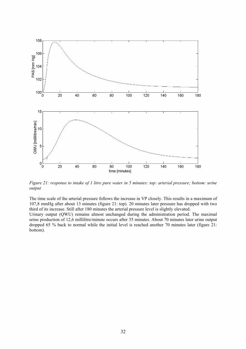
Figure 21: response to intake of 1 litre pure water in 5 minutes: top: arterial pressure; bottom: urine output The time scale of the arterial pressure follows the increase in VP closely. This results in a maximum of 107,8 mmHg after about 13 minutes (figure 21: top). 20 minutes later pressure has dropped with two third of its increase. Still after 180 minutes the arterial pressure level is slightly elevated. Urinary output (QWU) remains almost unchanged during the administration period. The maximal urine production of 12,6 millilitre/minute occurs after 35 minutes. About 70 minutes later urine output dropped 65 % back to normal while the initial level is reached another 70 minutes later (figure 21: bottom).

32

Figure 22: response to intake of 1 litre pure water in 5 minutes: top: plasma osmolality; bottom: Anti Diuretic Hormone & aldosteron The maximum decrease of plasma osmolality (OSMP) occurs 25 minutes after water intake started. This is about 10 minutes after maximal plasma volume is reached. After 50 minutes the OSMP level is elevated 65 % of the decreased value again while it takes about 110 minutes for the normal level (figure 22: top). The aldosteron (ALD) level becomes slightly smaller (-13 %) about 30 minutes after intake stopped, despite the 100-minutes buffer. The normal level is reached 90 minutes later (figure 22: bottom). The anti diuretic hormone (ADH) level is lowered considerably (-74 %) 50 minutes after infusion (figure 22: bottom). It takes about 60 minutes to regain two third of the ADH level and another 70 minutes to reach the normal level.

33

4. Discussion The major goal of this project was to construct a model which could be used to study body fluid regulation and blood volume control. Therefore a schematic model was developed (figure 5). However, implementation of this model is not possible at this moment since too many processes are not yet completely understood. This is especially the case for Atrial Natriuretic Factor and Brain Natriuretic Peptide. Moreover, it’s well possible that addition of ANF and BNP to existing models would require modifying parameter values of RAAS and ADH respectively. As a compromise, we choose to implement a model by Ikeda/Min. Later on, this model can be updated if necessary. Therefore an exploratory study was carried out to get an impression of the available possibilities.

§ 4.1 Explication of simulation results First it should be noted that our choice of the simulation cases was not perfect. In fact, two major determinants are being changed simultaneously: the osmolality of the administered fluid as well as the way of administration (orally/intravenously). This makes interpretation of the simulation results much more troublesome. Both simulations clearly illustrated the function of the various compartments. The plasma volume compartment serves as a location where the total fluid amount can be increased. Plasma volume returns back to normal within half an hour for the case of intravenous infusion as to retain a normal blood pressure value. Fluid redistribution occurs quickly to the interstitial spaces. Thereby the extra-cellular fluid compartment, and the interstitial fluid compartment in particular, serves as a volume buffer system. On the longer term fluid is being redistributed to the intra-cellular compartment. This is the only compartment where fluid administration can be observed hours after intravenous infusion or oral intake has taken place. Obviously, all redistribution processes occur faster for infusion than for oral intake since the level of volume increases are higher in this first case. We also found that arterial pressure increase is twice as great for saline infusion compared to water intake. Arterial pressure is a linear function of cardiac output [formula 3] and cardiac output is a linear function of blood volume [formula 2]. Thus the greater pressure increase is a direct consequence of the fluid administration method: for saline infusion this was done intravenously directly into the plasma volume instead of the oral administration which is carried out gradually (see § 2.2.4). The increase in urine output reached it’s maximum about 10 minutes earlier for saline infusion as a result of the faster volume increases. We expected a higher urine output for pure water loading since a lower plasma osmolality results in a decreased ADH output. However plasma osmolality turned out to be slightly lower for the administration of an iso-osmotic fluid, probably because in this case plasma volume reached a higher value thereby diluting the fluid. This resulted in a slightly higher ADH secretion (+10 %) for pure water. Aldosteron is known to increase sodium reabsorption (see § 1.1). Therefore administration of pure water should decrease aldosteron secretion, thus readjusting plasma osmolality. Aldosteron secretion is in this model, among others, made dependant on arterial pressure. For the case of saline infusion, a pressure increase of 16,4 % results in a maximal decrease in aldosteron level of 13 %. This magnitude seems reasonable. However, this value is reached after 35 minutes instead of the 100-minute delay period.

§ 4.2 Comparison of simulation results with literature reports The simulation results of the model by Ikeda/Min are now compared with literature values [6]. These values arise from the original model by Ikeda, who carried out the same experiments (figure 23). Plasma volume (VP) remains at a much higher level for the case of saline infusion in Ikeda’s report. The same holds for the interstitial volume (VIF) and thus for the sum of these, the extra-cellular

34

volume (VEC). It doesn’t seem logical that these volumes don’t return to their normal values. Remarkably, intra-cellular volume (VIC) remains completely unchanged. For the case of oral water intake, our simulation results are in good agreement with Ikeda’s results. Our response of arterial pressure (PAS) is in correspondence with the pressure increase found by Ikeda, in both cases. However we found a much higher urine output (QWU) for saline infusion. The total urine production observed by Ikeda is remarkably low. For the case of oral water intake, the maximum urine output was slightly higher in our simulation. The level of Anti Diuretic Hormone (ADH) reaches a much lower value in our simulation of saline infusion. This difference can be explained by looking at the plasma osmolality (OSMP), which remains constant in Ikeda’s research. For the oral intake of pure water a similar decrease in ADH was found. Ikeda did find a reasonable aldosteron decrease in both cases. Unlike with our results, this decrease takes place with the prescribed time delay of 100 minutes. Ikeda found a larger decrease for saline infusion. Thus, for pure water more sodium is reabsorbed.

Figure 23: Simulation of oral water loading (_____) and intravenous saline infusion (--------), both at a rate of 1 litre per 5 minutes. Also included is urine output of three human subjects (○ , ● and ∆) in case of oral water loading [6].

35

§ 4.3 Recommendations for future possibilities The implemented Ikeda/Min model has a wide variety of possibilities. First, the implementation of the aldosteron system should be checked. Probably, the time buffer isn’t programmed correctly. Future research should focus on a more thorough understanding of qualities and possibilities of this model. This can be done by performing additional simulation cases. Subjects could be administration of a fluid which keeps plasma osmolality constant, or administration of a fluid with an elevated osmolality level (“sea water”). These cases should be carried out orally as well as intravenously. Thus, better understanding of aldosteron and anti diuretic hormone characteristics is reached. Next, the model can be extended with a more detailed description of circulation. Heart dynamics are coupled now to the renal system. Anatomically this can be accomplished via afferent and efferent arterioles. Special attention should be on time scale differences in regulating processes like short-term heart rate adjustment (~ minutes) and intermediate term body fluid regulation (~ 1 hour). The value of adding atrial natriuretic factor and brain natriuretic peptide should be investigated. Finally, fundamental research on problems arising with heart failure is possible. Also the influence of typical water and salt diets can be investigated. Concrete clinical problems are more difficult to examine since the model is based on a 55 kg male. Thus, differences in fluid distribution resulting from weight variances are not taken into account yet. Also, water and salt regulation is in reality gender dependant as a result of differences in average lean body mass [1].

36

Conclusion This preliminary study for the control of body fluids forms the basis for further research. Already insight in relevant physiological processes is deepened greatly. The development of a model containing all characteristics, necessary for studying heart failure, is still troublesome. However a good alternative is found in the model by Ikeda/Min [6]. This model lacks some characteristics as defined in figure 5 (ANF, BNP, explicit circulatory blood flow) but has the advantage of having incorporated various ion concentrations. Thereby osmotic processes can be modelled realistically with this model. However, some constants and variables might need some readjustment. This depends on testing results not yet available. Still the Ikeda/Min model has to be extended with heart dynamics. A schematic diagram, closely connected to the lay-out of the model by Arts [2003], forms the first step in developing such a model (see Appendix V). Ultimately, this extended model will be used for research on heart failure. Particularly, the use of water and salt diets, commonly used in clinical practice now, can be investigated.

37

Appendix I: References [1] Bernards J.A., Bouman L.N., Fysiologie van de mens, Houten: Bohn Stafleu Van Loghum,

1994 [2] Dickinson C.J., Ingram D., Shephard P., A digital computer model for teaching the principles

of systemic haemodynamics (“MacMan”), Proceedings of the physiological society, 9-10, 1971

[3] Dickinson C.J., Shephard P., A digital computer model of the systemic circulation and kidney, for studying renal and circulatory interactions involving electrolytes and body fluid compartments (“MacPee”), Proceedings of the physiological society, 11-12, 1971

[4] Guyton A.C., Hall J.E., Textbook of medical physiology, Pennsylvania: W.B. Saunders company, 1996

[5] Guyton A.C., Coleman T.G., Jones C.E., Circulatory physiology: cardiac output and its regulation, London: Saunders, 1973

[6] Ikeda N., Marumo F., Shirataka M., Sato T., A model of overall regulation of body fluids, Annals of Biomedical Engineering, 7: 135-166, 1979

[7] Jensen K.T., Carstens J., Pedersen E.B., Effect of BNP on renal hemodynamics, tubular function and vasoactive hormones in humans (abstract), American journal of physiology (Renal physiology), 274: 63, 1998

[8] Keener J., Sneyd J., Mathematical physiology, New York: Springer-Verlag, 1998 [9] La Villa G. et al., Acute effects of physiological increments of Brain Natriuretic Peptide in

Humans, Hypertension, 26: 628-633, 1995 [10] Min F.B.M., Computersimulatie en wiskundige modellen in het medisch onderwijs,

Maastricht: Rijksuniversiteit Limburg, 1982 [11] Moore L.C., Rich A., Casellas D., Ascending myogenic autoregulation: interactions between

tubuloglomerular feedback and myogenic mechanisms, Bulletin of mathematical biology, 56: 391-410, 1994

[12] Roelandt J.R.T.C., Lie K.I., Wellens H.J.J., Van de Werf F., Leerboek cardiologie, Houten: Bohn Stafleu Van Loghum, 1995

[13] Schmidt R.F., Thews G., Human physiology, Berlin: Springer, 1989 [14] Van der Zander K. et al., Does Brain Natriuretic Peptide have a direct renal effect in human

hypertensives? (abstract), Hypertension, 41: 119, 2003 [15] Van Wijk van Brievingh R.P., Möller D.P.F., Biomedical Modeling and simulation on a PC,

New York: Springer-Verlag, 1993 [16] http://people.msoe.edu/~barnicks/courses/cs400/19967/renal/webmodel.pdf[17] http://www.chime.ucl.ac.uk/resources/Models/macpee.htm[18] http://projects.edte.utwente.nl/pi/Book?H9Cardio.htm

38

Appendix II: Implementation of model for fluid regulation by Ikeda/Min This chapter explains the lay-out used in the programming MATLAB code. Each block, as described in chapter § 2.2, is placed in a separate M-file. These M-files are all functions called upon in a central controlling M-file, called main.m. All input-variables defined in these function-statements are calculated in another block, while all defined output-variables will be used in other blocks. This organization also follows directly from figure 7 in chapter § 2.2. The time-loop is also placed in main.m. In each loop, all blocks are called upon in their own M-file. At the start of the simulation, initial conditions are loaded from init.m. This can be done either via main.m, if they are an input-variable in one or more of the blocks, or via a special array if they were not imported previously by main.m. These special arrays containing initial conditions are named after the concerning block according to the following convention: Start* with the asterix referring to the name of a function. The structure “Stat.*” contains all variables necessary for continuing a previous simulation, with the asterix now indicating a variable name. Concurrently, this Stat.*-structure is also used for the visualization of the simulation results in Stat2Graph.m. Finally, each capital “F” occurring in the comment lines refers to mathematical functions defined in Appendix III of [6]. FNTML.m is programmed as a separate function since the concerning Tm-limited function is used quite often.

39

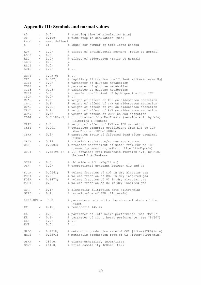
Appendix III: Symbols and normal values t0 = 0.0; % starting time of simulation (min) DT = 0.199; % time step in simulation (min) tend = user defined i = 1; % index for number of time loops passed ADH = 1.0; % effect of antidiuretic hormone (ratio to normal) ADH0 = 0.0; % ALD = 1.0; % effect of aldosteron (ratio to normal) ALD0 = 0.0; % ALD1 = 0.0; % ACTH = 1.0; % ... CBFI = 1.0e-9; % ... CFC = 0.007; % capillary filtration coefficient (liter/min/mm Hg) CGL1 = 1.0; % parameter of glucose metabolism CGL2 = 1.0; % parameter of glucose metabolism CGL3 = 0.03; % parameter of glucose metabolism CHEI = 5.0; % transfer coefficient of hydrogen ion into ICF CION = 0.0; % ... CKAL = 0.5; % weight of effect of XKE on aldosteron secretion CNAL = 0.1; % weight of effect of YNH on aldosteron secretion CPAL = 0.01; % weight of effect of PAS on aldosteron secretion CPVL = 0.1; % weight of effect of PVP on aldosteron secretion COAD = 0.5; % weight of effect of OSMP on ADH secretion CORG = 5.01189e-5; % ... obtained from MacThesis (version 4.1) by Min,

Reimerink & Renkema CPAD = 1.0; % weight of effect of PVP on ADH secretion CKEI = 0.001; % potassium transfer coefficient from ECF to ICF

(MacThesis: CKEI=0.0007) CPRX = 0.2; % excretion ratio of filtered load after proximal

tubule CRAV = 5.93; % arterial resistance/venous resistance CSM = 0.0003; % transfer coefficient of water from ECF to ICF

caused by osmotic gradient (liter^2/mEq/min) CPO4 = 1.5849e-7; % ... obtained from MacThesis (version 4.1) by Min,

Reimerink & Renkema DCLA = 0.0; % chloride shift (mEq/liter) DEN = 1.0; % proportional constant between QCO and VB FCOA = 0.0561; % volume fraction of CO2 in dry alveolar gas FCOI = 0.0; % volume fraction of CO2 in dry inspired gas FO2A = 0.1473; % volume fraction of O2 in dry alveolar gas FO2I = 0.21; % volume fraction of O2 in dry inspired gas GFR = 0.1; % glomerular filtration rate (litre/min) GFR0 = 0.1; % normal value of GFR (litre/min) %HF0-HF4 = 0.0; % parameters related to the abnormal state of the

heart HT = 0.45; % hematocrit (45 %) KL = 0.2; % parameter of left heart performance (see "PVP0") KR = 0.3; % parameter of right heart performance (see "PVS0") KLF = 1.0; % ... KVI = 0.0; % ... MRCO = 0.2318; % metabolic production rate of CO2 [liter(STPD)/min] MRO2 = 0.2591; % metabolic production rate of O2 [liter(STPD)/min] OSMP = 287.0; % plasma osmolality (mOsm/liter) OSMU = 461.0; % urine osmolality (mOsm/liter)

40

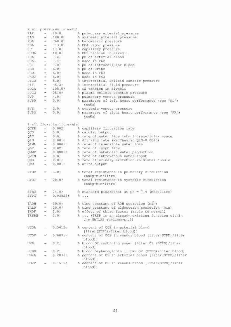
% all pressures in mmHg! PAP = 20.0; % pulmonary arterial pressure PAS = 100.0; % systemic arterial pressure PBA = 760.0; % barometric pressure PBL = 713.0; % PBA-vapor pressure PC = 17.0; % capillary pressure PCOA = 40.0; % CO2 tension in alveoli PHA = 7.4; % pH of arterial blood PHA1 = 7.4; % used in F62 PHI = 7.0; % pH of intracellular blood PHU = 6.0; % pH of urine PHU1 = 6.0; % used in F63 PHU2 = 6.0; % used in F63 PICO = 5.0; % interstitial colloid osmotic pressure PIF = -6.3; % interstitial fluid pressure PO2A = 105.0; % O2 tension in alveoli PPCO = 28.0; % plasma colloid osmotic pressure PVP = 4.0; % pulmonary venous pressure PVP0 = 0.0; % parameter of left heart performance (see "KL")

(mmHg) PVS = 3.0; % systemic venous pressure PVSO = 0.0; % parameter of right heart performance (see "KR")

(mmHg) % all flows in litre/min! QCFR = 0.002; % capillary filtration rate QCO = 5.0; % cardiac output QIC = 0.0; % rate of water flow into intracellular space QIN = 0.001; % drinking rate (MacThesis: QIN=0.0015) QIWL = 0.0005; % rate of insensible water loss QLF = 0.02; % rate of lymph flow QMWP = 0.0005; % rate of metabolic water production QVIN = 0.0; % rate of intravenous water input QWD = 0.01; % rate of urinary excretion in distal tubule QWU = 0.001; % urine output RTOP = 3.0; % total resistance in pulmonary circulation

(mmHg*min/litre) RTOT = 20.0; % total resistance in systemic circulation

(mmHg*min/litre) STBC = 24.0; % standard bicarbonat at pH = 7.4 (mEq/litre) STPG = 0.03823; % ... TADH = 30.0; % time constant of ADH secretion (min) TALD = 30.0; % time constant of aldosteron secretion (min) THDF = 1.0; % effect of third factor (ratio to normal) TRSPN = 2.0; % ... (TRSP is an already existing function within

the MATLAB environment!) UCOA = 0.5612; % content of CO2 in arterial blood

[liter(STPD)/liter blood)] UCOV = 0.6075; % content of CO2 in venous blood [liter(STPD)/liter

blood)] UHB = 0.2; % blood O2 combining power [liter O2 (STPD)/liter

blood] UHB0 = 0.2; % blood oxyhemoglobin [liter 02 (STPD)/liter blood] UO2A = 0.2033; % content of O2 in arterial blood [liter(STPD)/liter

blood)] UO2V = 0.1515; % content of O2 in venous blood [liter(STPD)/liter

blood)]

41

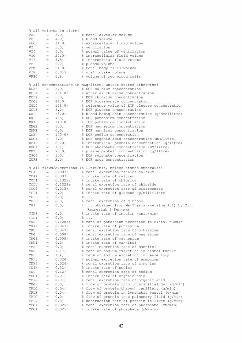
% all volumes in litre! VAL = 3.0; % total alveolar volume VB = 4.0; % blood volume VEC = 11.0; % extracellular fluid volume VI = 5.0; % ventilation VI0 = 5.0; % normal value of ventilation VIC = 20.0; % intracellular fluid volume VIF = 8.8; % interstitial fluid volume VP = 2.2; % plasma volume VTW = 31.0; % total body fluid volume VIN = 0.015; % oral intake volume VRBC = 1.8; % volume of red blood cells % all concentrations in mEq/litre, unless stated otherwise! XCAE = 5.0; % ECF calcium concentration XCLA = 104.0; % arterial chloride concentration XCLE = 6.0; % ECF chloride concentration XCO3 = 24.0; % ECF bicarbonate concentration XGL0 = 108.0; % reference value of ECF glucose concentration XGLE = 6.0; % ECF glucose concentration XHB = 15.0; % blood hemaglobin concentration (g/decilitre) XKE = 4.5; % ECF potassium concentration XKI = 140.0; % ICF potassium concentration XMGE = 3.0; % ECF magnesium concentration XMNE = 0.0; % ECF mannitol concentration XNE = 140.0; % ECF sodium concentration XOGE = 6.0; % ECF organic acid concentration (mM/litre) XPIF = 20.0; % interstitial protein concentration (g/litre) XPO4 = 1.1; % ECF phosphate concentration (mM/litre) XPP = 70.0; % plasma protein concentration (g/litre) XSO4 = 1.0; % ECF sulphate concentration XURE = 2.5; % ECF urea concentration % all flows/excretions in litre/min, unless stated otherwise! YCA = 0.007; % renal excretion rate of calcium YCAI = 0.007; % intake rate of calcium YCLI = 0.1328; % intake rate of chloride YCLU = 0.1328; % renal excretion rate of chloride YCO3 = 0.015; % renal excretion rate of bicarbonate YGLI = 0.0; % intake rate of glucose (g/millilitre) YGLS = 0.0; % ... YGLU = 0.0; % renal excretion of glucose YHI = 0.0; % ... obtained from MacThesis (version 4.1) by Min,

Reimerink & Renkema YINS = 0.0; % intake rate of insulin (unit/min) YINT = 0.0; % ... YKD = 0.1205; % rate of potassium excretion in distal tubule YKIN = 0.047; % intake rate of potassium YKU = 0.047; % renal excretion rate of potassium YMG = 0.008; % renal excretion rate of magnesium YMGI = 0.008; % intake rate of magnesium YMNI = 0.0; % intake rate of mannitol YMNU = 0.0; % renal excretion rate of mannitol YND = 1.17; % rate of sodium excretion in distal tubule YNH = 1.4; % rate of sodium excretion in Henle loop YNH0 = 0.024; % normal excretion rate of ammonium YNH4 = 0.024; % renal excretion rate of ammonium YNIN = 0.12; % intake rate of sodium YNU = 0.12; % renal excretion rate of sodium YOGI = 0.01; % intake rate of organic acid YORG = 0.01; % renal excretion rate of organic acid YPG = 0.0; % flow of protein into interstitial gel (g/min) YPLC = 0.04; % flow of protein through capillary (g/min) YPLF = 0.04; % flow of protein in lymphatic vessel (g/min) YPLG = 0.0; % flow of protein into pulmonary fluid (g/min) YPLV = 0.0; % destruction rate of protein in liver (g/min) YPO4 = 0.025; % renal excretion rate of phosphate (mM/min) YPOI = 0.025; % intake rate of phosphate (mM/min)

42

YSO4 = 0.02; % renal excretion rate of sulphate YSOI = 0.02; % intake rate of sulphate YTA = 0.0168; % renal excretion rate of titratable acid YTA0 = 0.0068; % normal excretion rate of titratable acid YURI = 0.15; % intake rate of urea YURU = 0.15; % renal excretion rate of urea % all contents in mEq, unless stated otherwise! ZCAE = 55.0; % ECF calcium content ZCLE = 1144.0; % ECF chloride content ZKE = 49.5; % ECF potassium content ZKI = 2800.0; % ICF potassium content ZMGE = 33.0; % ECF magnesium content ZMNE = 0.0; % ECF mannitol content ZNE = 1540.0; % ECF sodium content ZOGE = 66.0; % ECF organic acid content (mM) ZPG = 20.0; % protein content in interstitial gel (g) ZPIF = 176.0; % ISF protein content (g) ZPLG = 70.0; % protein content in pulmonary fluid (g) ZPO4 = 12.1; % ECF phosphate content (mM) ZPP = 154.0; % plasma protein content (g) ZSO4 = 11.0; % ECF sulphate content ZURE = 77.5; % ECF urea content ZHI = 100.0; % ... ZGLE = 66.0; % ECF glucose content ZSOE = 11.0; % ECF sulphate content ZPOE = 22.0; % ECF phosphate content

43

Appendix IV: Specifications for two cases of disturbed fluid balance In order to be able to illustrate the model, several cases which can be compared with experimental and/or literal data have been build. Case I: Iso-osmotic saline infusion In this simulation physiological saline is infused intravenously at a rate of 1 litre per 5 minutes. QVIN = 0,2 litre/min YNIN = 31 mEq/min YCLI = 31 mEq/min The simulation time is automatically reset to 5 minutes, but can be changed on demand in init.m After this water administration an additional simulation must be performed using the last calculated values. Usually, the response is calculated for a period of 3 hours: CaseNr = 2 tend = 175 min Case II: Pure water loading In this simulation, oral water intake of 0,2 litre/minute is simulated during 5 minutes, compared to a normal intake of 0,001. QIN = 0,2 litre/min Thus, loading of 1 litre of pure water is accomplished. Again the simulation time is reset to 5 minutes and the response is calculated for a period of 180 minutes. Of course many other cases can be tested, like respiratory responses to increased PCO2 and decreased PO2, glucose metabolism and potassium, metabolic acid-base disturbances and intra-cellular buffering, respiratory acid-base disturbances and compensation by the kidney, etc. [6, 10, 15].

44

Appendix V: Lumped parameter model In this section the electrical equivalent model (see figure 24) of the renal feedback mechanism diagram for the control of blood volume, as presented in figure 5, will be derived. This thus forms a first attempt to translate the theoretical model to the Matlab environment. Eventually, this electric diagram can be implemented then into the lumped parameter model by Theo Arts [2003, TUE/UM]. The renal fluid control model is constructed out of the following modules:

Tube (artery/vein) Volume compartment Heart valve Resistance Black box

45

Figure 24: schematic representation of the lumped parameter model Nomenclature: Hemodynamics Subscripts p Pa pressure int interstitial compartment q litre/min flow trough vessels or valves sv systemic vein R Pa•min/litre circulatory resistance mt mitral valve Z Pa•min/litre characteristic input impedance ao aorta

of the circulation tsa tube systemic artery tsv tube systemic vein Abbreviations p peripheral Fin inflow of fluid aff afferent arteriole Fout outflow of fluid eff efferent arteriole glom Glomerulus abs reabsorption tub Tubule exc excretion blad Bladder rt renal total

46