Renewable Energy Tariff and Financial Analysis Tool

Renewable Energy Tariff and Financial Analysis Tool

User Guide

Prayas Energy Group, PuneSeptember 2014

Renewable Energy Tariff and Financial Analysis Tool

User Guide

Shweta Kulkarni, Srihari Dukkipati and Ashwin Gambhir

Prayas Energy Group,

III A&B, Devgiri, Kothrud Industrial Area

Joshi Museum Lane, Kothrud, Pune – 411038

Telephone: +(91) 20-2542 0720, 6520 5726, Fax: 2543 9134

Email: [email protected]

Website: http://www.prayaspune.org/peg

Renewable Energy Tariff and Financial Analysis Tool User Guide v2.0

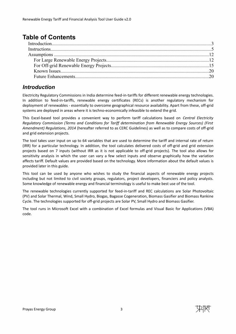
Table of ContentsIntroduction......................................................................................................................................3Instructions.......................................................................................................................................5Assumptions ..................................................................................................................................12

For Large Renewable Energy Projects......................................................................................12For Off-grid Renewable Energy Projects..................................................................................15Known Issues............................................................................................................................20Future Enhancements................................................................................................................20

IntroductionElectricity Regulatory Commissions in India determine feed-in-tariffs for different renewable energy technologies.In addition to feed-in-tariffs, renewable energy certificates (RECs) is another regulatory mechanism fordeployment of renewables - essentially to overcome geographical resource availability. Apart from these, off-gridsystems are deployed in areas where it is techno-economically infeasible to extend the grid.

This Excel-based tool provides a convenient way to perform tariff calculations based on Central ElectricityRegulatory Commission (Terms and Conditions for Tariff determination from Renewable Energy Sources) (FirstAmendment) Regulations, 2014 (hereafter referred to as CERC Guidelines) as well as to compare costs of off-gridand grid extension projects.

The tool takes user input on up to 64 variables that are used to determine the tariff and internal rate of return(IRR) for a particular technology. In addition, the tool calculates delivered costs of off-grid and grid extensionprojects based on 7 inputs (without IRR as it is not applicable to off-grid projects). The tool also allows forsensitivity analysis in which the user can vary a few select inputs and observe graphically how the variationaffects tariff. Default values are provided based on the technology. More information about the default values isprovided later in this guide.

This tool can be used by anyone who wishes to study the financial aspects of renewable energy projectsincluding but not limited to civil society groups, regulators, project developers, financiers and policy analysts.Some knowledge of renewable energy and financial terminology is useful to make best use of the tool.

The renewable technologies currently supported for feed-in-tariff and REC calculations are Solar Photovoltaic(PV) and Solar Thermal, Wind, Small Hydro, Biogas, Bagasse Cogeneration, Biomass Gasifier and Biomass RankineCycle. The technologies supported for off-grid projects are Solar PV, Small Hydro and Biomass Gasifier.

The tool runs in Microsoft Excel with a combination of Excel formulas and Visual Basic for Applications (VBA)code.

Prayas Energy Group 3


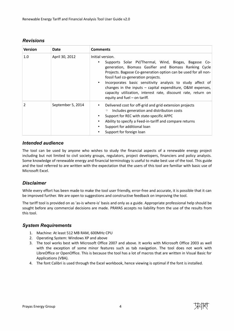
Revisions

Version Date Comments

1.0 April 30, 2012 Initial version.• Supports Solar PV/Thermal, Wind, Biogas, Bagasse Co-

generation, Biomass Gasifier and Biomass Ranking CycleProjects. Bagasse Co-generation option can be used for all non-fossil fuel co-generation projects.

• Incorporates basic sensitivity analysis to study affect ofchanges in the inputs – capital expenditure, O&M expenses,capacity utilization, interest rate, discount rate, return onequity and fuel – on tariff.

2 September 5, 2014 • Delivered cost for off-grid and grid extension projects◦ Includes generation and distribution costs

• Support for REC with state-specific APPC• Ability to specify a Feed-in-tariff and compare returns• Support for additional loan• Support for foreign loan

Intended audience

The tool can be used by anyone who wishes to study the financial aspects of a renewable energy projectincluding but not limited to civil society groups, regulators, project developers, financiers and policy analysts.Some knowledge of renewable energy and financial terminology is useful to make best use of the tool. This guideand the tool referred to are written with the expectation that the users of this tool are familiar with basic use ofMicrosoft Excel.

Disclaimer

While every effort has been made to make the tool user friendly, error-free and accurate, it is possible that it canbe improved further. We are open to suggestions and constructive feedback on improving the tool.

The tariff tool is provided on as 'as-is where-is' basis and only as a guide. Appropriate professional help should besought before any commercial decisions are made. PRAYAS accepts no liability from the use of the results fromthis tool.

System Requirements

1. Machine: At least 512 MB RAM, 600MHz CPU2. Operating System: Windows XP and above3. The tool works best with Microsoft Office 2007 and above. It works with Microsoft Office 2003 as well

with the exception of some minor features such as tab navigation. The tool does not work withLibreOffice or OpenOffice. This is because the tool has a lot of macros that are written in Visual Basic forApplications (VBA).

4. The font Calibri is used through the Excel workbook, hence viewing is optimal if the font is installed.



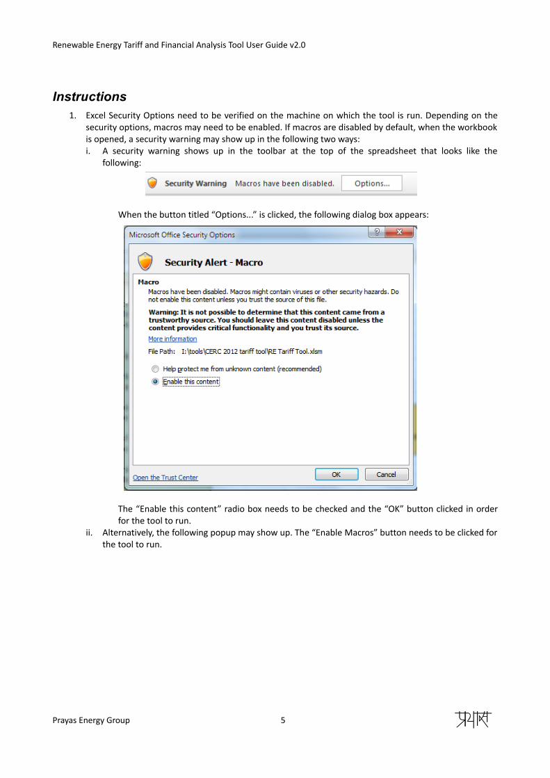
Instructions1. Excel Security Options need to be verified on the machine on which the tool is run. Depending on the

security options, macros may need to be enabled. If macros are disabled by default, when the workbookis opened, a security warning may show up in the following two ways:i. A security warning shows up in the toolbar at the top of the spreadsheet that looks like the

following:

When the button titled “Options...” is clicked, the following dialog box appears:

The “Enable this content” radio box needs to be checked and the “OK” button clicked in orderfor the tool to run.

ii. Alternatively, the following popup may show up. The “Enable Macros” button needs to be clicked forthe tool to run.



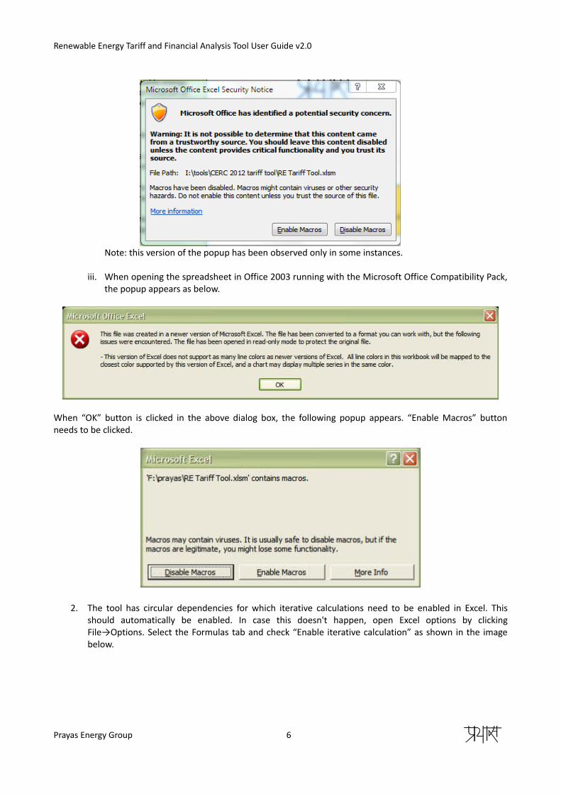
Note: this version of the popup has been observed only in some instances.

iii. When opening the spreadsheet in Office 2003 running with the Microsoft Office Compatibility Pack,the popup appears as below.

When “OK” button is clicked in the above dialog box, the following popup appears. “Enable Macros” buttonneeds to be clicked.

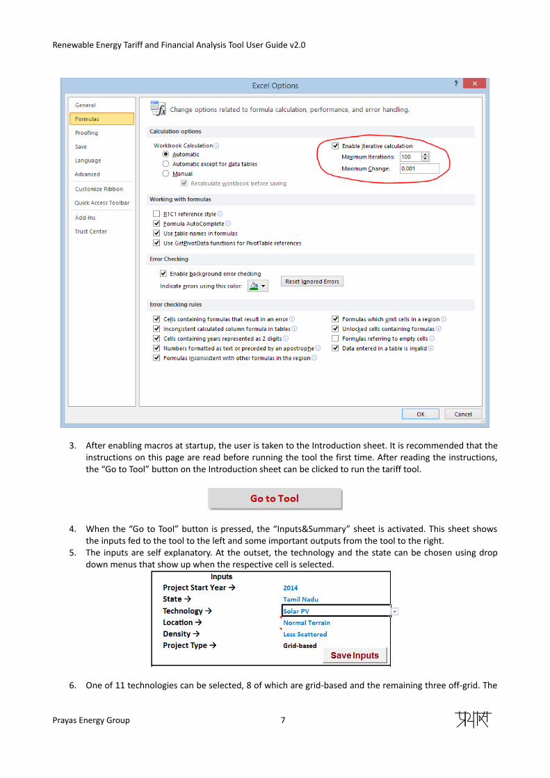
2. The tool has circular dependencies for which iterative calculations need to be enabled in Excel. Thisshould automatically be enabled. In case this doesn't happen, open Excel options by clickingFile→Options. Select the Formulas tab and check “Enable iterative calculation” as shown in the imagebelow.



3. After enabling macros at startup, the user is taken to the Introduction sheet. It is recommended that theinstructions on this page are read before running the tool the first time. After reading the instructions,the “Go to Tool” button on the Introduction sheet can be clicked to run the tariff tool.

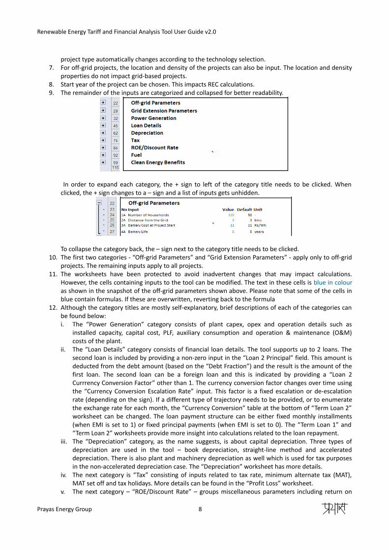
4. When the “Go to Tool” button is pressed, the “Inputs&Summary” sheet is activated. This sheet showsthe inputs fed to the tool to the left and some important outputs from the tool to the right.

5. The inputs are self explanatory. At the outset, the technology and the state can be chosen using dropdown menus that show up when the respective cell is selected.

6. One of 11 technologies can be selected, 8 of which are grid-based and the remaining three off-grid. The



project type automatically changes according to the technology selection.7. For off-grid projects, the location and density of the projects can also be input. The location and density

properties do not impact grid-based projects.8. Start year of the project can be chosen. This impacts REC calculations.9. The remainder of the inputs are categorized and collapsed for better readability.

In order to expand each category, the + sign to left of the category title needs to be clicked. Whenclicked, the + sign changes to a – sign and a list of inputs gets unhidden.

To collapse the category back, the – sign next to the category title needs to be clicked.10. The first two categories - “Off-grid Parameters” and “Grid Extension Parameters” - apply only to off-grid

projects. The remaining inputs apply to all projects.11. The worksheets have been protected to avoid inadvertent changes that may impact calculations.

However, the cells containing inputs to the tool can be modified. The text in these cells is blue in colouras shown in the snapshot of the off-grid parameters shown above. Please note that some of the cells inblue contain formulas. If these are overwritten, reverting back to the formula

12. Although the category titles are mostly self-explanatory, brief descriptions of each of the categories canbe found below:i. The “Power Generation” category consists of plant capex, opex and operation details such as

installed capacity, capital cost, PLF, auxiliary consumption and operation & maintenance (O&M)costs of the plant.

ii. The “Loan Details” category consists of financial loan details. The tool supports up to 2 loans. Thesecond loan is included by providing a non-zero input in the “Loan 2 Principal” field. This amount isdeducted from the debt amount (based on the “Debt Fraction”) and the result is the amount of thefirst loan. The second loan can be a foreign loan and this is indicated by providing a “Loan 2Currrency Conversion Factor” other than 1. The currency conversion factor changes over time usingthe “Currency Conversion Escalation Rate” input. This factor is a fixed escalation or de-escalationrate (depending on the sign). If a different type of trajectory needs to be provided, or to enumeratethe exchange rate for each month, the “Currency Conversion” table at the bottom of “Term Loan 2”worksheet can be changed. The loan payment structure can be either fixed monthly installments(when EMI is set to 1) or fixed principal payments (when EMI is set to 0). The “Term Loan 1” and“Term Loan 2” worksheets provide more insight into calculations related to the loan repayment.

iii. The “Depreciation” category, as the name suggests, is about capital depreciation. Three types ofdepreciation are used in the tool – book depreciation, straight-line method and accelerateddepreciation. There is also plant and machinery depreciation as well which is used for tax purposesin the non-accelerated depreciation case. The “Depreciation” worksheet has more details.

iv. The next category is “Tax” consisting of inputs related to tax rate, minimum alternate tax (MAT),MAT set off and tax holidays. More details can be found in the “Profit Loss” worksheet.

v. The next category – “ROE/Discount Rate” – groups miscellaneous parameters including return on



equity (ROE) expected for the project, discount rate calculated based on the post-tax ROE andassociated annuity factor.

vi. The “Fuel” category only applies to biomass-based projects, i.e., biogas, bagasse and biomassgasifier. This includes fuel requirement, fuel cost and fuel cost escalation. In addition, there are acouple of parameters – “Duration of initial CUF” and “CUF for subsequent years” – for biomassrankine cycle projects which have a lower CUF in the first two years.

vii. The last category – “Clean Energy Benefits” – lists inputs related to the financial incentives availableto clean energy projects. This includes REC, feed-in tariffs and carbon trading incomes.

13. Finally the “Save Inputs” button can be used to save the current set of inputs for the selectedtechnology. This may not be useful if the default values provided are used as inputs, but if any of theinputs are changed, they can be saved off so that when the same technology is used next time, thoseinputs are filled in.

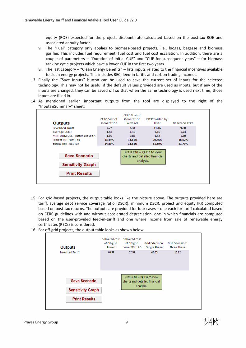
14. As mentioned earlier, important outputs from the tool are displayed to the right of the“Inputs&Summary” sheet.

15. For grid-based projects, the output table looks like the picture above. The outputs provided here aretariff, average debt service coverage ratio (DSCR), minimum DSCR, project and equity IRR computedbased on post-tax returns. The outputs are provided for four cases – one each for tariff calculated basedon CERC guidelines with and without accelerated depreciation, one in which financials are computedbased on the user-provided feed-in-tariff and one where income from sale of renewable energycertificates (RECs) is considered.

16. For off-grid projects, the output table looks as shown below.



Here, the first two columns show the delivered per-unit cost of the off-grid project including generation,distribution and maintenance costs. These numbers are influenced by the number of households andterrain of the region served. The next two columns show estimated electricity tariffs for single phase andthree phase grid extension to that region. A three phase grid connection is expected to supportincreased productive load; hence the per unit tariff would be lower.

17. As can be seen, there are 3 additional buttons in the output box – “Save Scenario”, “Sensitivity Graph”and “Print Results”. These are described below.

18. “Save Scenario” saves most of the inputs and outputs from the current run. Upto 10 runs can be saved.The runs are saved in the “Scenarios” sheet. The user is prompted to enter a scenario index (1-10) andaccordingly the inputs and outputs are saved in the corresponding column in the “Scenarios” sheet.

19. The “Tariff Chart” displays a graph depicting the different components of the tariff resulting from theprovided inputs. The levelized tariff with and without accelerated depreciation is also shown in thisgraph. Another view of the same is shown in the “Tariff breakup Chart”.

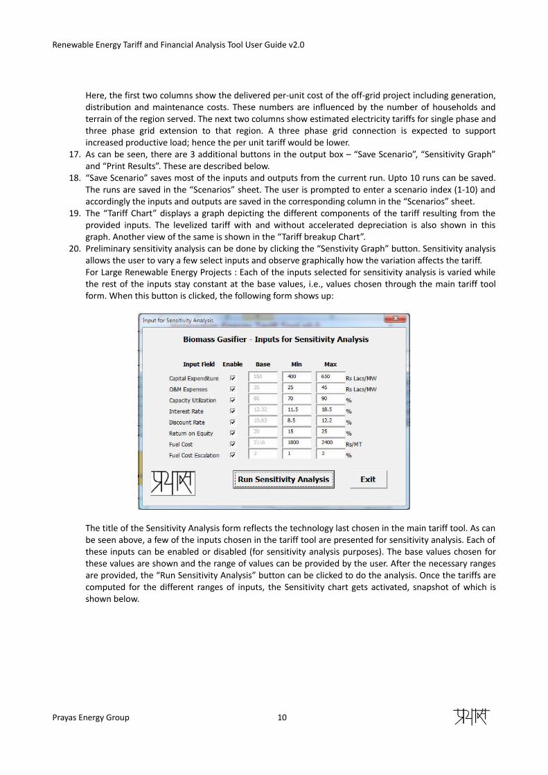
20. Preliminary sensitivity analysis can be done by clicking the “Senstivity Graph” button. Sensitivity analysisallows the user to vary a few select inputs and observe graphically how the variation affects the tariff. For Large Renewable Energy Projects : Each of the inputs selected for sensitivity analysis is varied whilethe rest of the inputs stay constant at the base values, i.e., values chosen through the main tariff toolform. When this button is clicked, the following form shows up:

The title of the Sensitivity Analysis form reflects the technology last chosen in the main tariff tool. As canbe seen above, a few of the inputs chosen in the tariff tool are presented for sensitivity analysis. Each ofthese inputs can be enabled or disabled (for sensitivity analysis purposes). The base values chosen forthese values are shown and the range of values can be provided by the user. After the necessary rangesare provided, the “Run Sensitivity Analysis” button can be clicked to do the analysis. Once the tariffs arecomputed for the different ranges of inputs, the Sensitivity chart gets activated, snapshot of which isshown below.



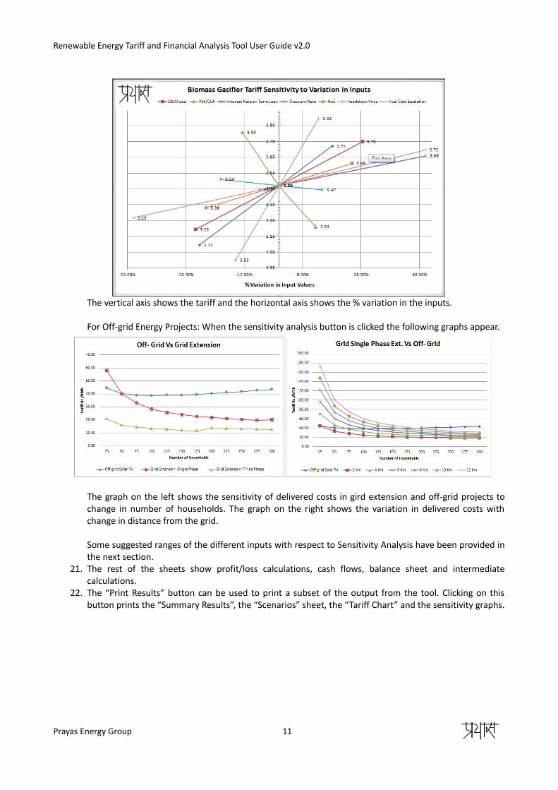
The vertical axis shows the tariff and the horizontal axis shows the % variation in the inputs.

For Off-grid Energy Projects: When the sensitivity analysis button is clicked the following graphs appear.

The graph on the left shows the sensitivity of delivered costs in gird extension and off-grid projects tochange in number of households. The graph on the right shows the variation in delivered costs withchange in distance from the grid.

Some suggested ranges of the different inputs with respect to Sensitivity Analysis have been provided inthe next section.

21. The rest of the sheets show profit/loss calculations, cash flows, balance sheet and intermediatecalculations.

22. The “Print Results” button can be used to print a subset of the output from the tool. Clicking on thisbutton prints the “Summary Results”, the “Scenarios” sheet, the “Tariff Chart” and the sensitivity graphs.



Assumptions

For Large Renewable Energy Projects

Default Values

1. The default capacity utilization factor (CUF also referred to as plant load factor, PLF) for Wind has beentaken as 25% in the tool. Per CERC Guidelines Regulation 26(1), the following CUF values arerecommended based on the wind power density of the project. It is left to the user to enter theappropriate CUF.

Annual Mean Wind PowerDensity (W/m2)

CUF

Upto 200 20%

201-250 22%

251-300 25%

301-400 30%

> 400 32%

2. The default capital cost for small hydro projects (SHP) has been taken as Rs 700 lacs/MW. Per CERCGuidelines Regulation 28(1), the following capital costs are recommended based on the hoststate/region and capacity of the hydro power project. It is left to the user to enter the appropriatecapital cost based on the following table:

Region Project Size Capital Cost(Rs Lacs/MW)

CUF O&M Expenses(Rs Lacs/MW)

Himachal Pradesh, Uttarakhand andNorth Eastern States

Below 5 MW 770 45.00% 25

5 to 25 MW 700 45.00% 18

Other StatesBelow 5 MW 600 30.00% 20

5 to 25 MW 550 30.00% 14

3. The default CUF for small hydro projects provided in the tool is 45%. According to CERC GuidelinesRegulation 30, the normative CUF is 45% for Himachal Pradesh, Uttarakhand and North Eastern Statesand 30% for other states. In addition, the CERC Guidelines state that the “normative CUF is net of freepower to the home state if any, and any quantum of free power if committed by the developer over andabove the normative CUF shall not be factored into the tariff.” The user needs to enter the appropriateCUF based on this regulation.

4. Likewise, default O&M expense for small hydro projects is taken as Rs 25 Lakhs/MW. The O&M expensesneed to be modified according to above table.

5. With reference to biomass rankine cycle projects, CERC Guidelines Regulation 41 states this: “The use offossil fuels shall be limited to the extent of 15% of total fuel consumption on annual basis.” However, thetool does not have a provision to enter a fossil fuel input. This will be considered for a future update ofthe tool.

6. According to the CERC Guidelines Regulation 44 (updated for 2014-15 as per Suo Motu order 354), state-wise normative feedstock prices for biomass (gasifier and rankine cycle) projects are as follows. The toolpicks these value based on the selected state.



State Biomass PriceRs/tonne

Andhra Pradesh 2747.59

Haryana 3127.4

Maharashtra 3198.61

Punjab 3271.01

Rajasthan 2729.79

Tamil Nadu 2702.49

UP 2795.07

Other States 2938.69

7. The default fuel requirement for biomass rankine cycle projects is 1.331 kg/kWh. This is calculated fromthe normative values of Station Heat Rate of 4125 kCal/kWh for projects using AFBC boiler and Calorificvalue of 3100 kCal/kg as per 1st Amendment to the CERC regulation, 2014. Earlier recommended valueswere 4000 kCal/kWh (Regulation 38) and 3300 kCal/kg (Regulation 43) respectively which translate to afuel requirement 1.212 kg/Kwh.

8. For co-generation projects, a default CUF of 53% has been used. The normative values provided in theCERC Guidelines are as follows:

State Operating Days Plant LoadFactor (%)

Uttar Pradeshand AndhraPradesh

120 days (crushing) + 60 days (off-season) = 180 days operating days

45%

Tamil Nadu andMaharashtra

180 days (crushing) + 60 days (off-season) = 240 days operating days

60%

Other States 150 days (crushing) + 60 days (off-season) = 210 days operating days

53%

9. For co-generation projects, the default fuel requirement is 1.6 kg/kWh. This is calculated from thenormative values of Station Heat Rate (Regulation 51: 3600 kCal/kWh) and Calorific Value (Regulation52: 2250 kCal/kg) provided in the CERC Guidelines.

10. The default fuel escalation rate for biomass rankine cycle, bagasse co-generation and biomass gasifierprojects is 5% as per CERC Guidelines - Regulations 44, 53 and 73. Please note that this results in errorsin IRR calculations by Excel (please see point #3 in the Calculations section below).

11. For biomass gasifier and biogas projects, capital subsidy has been assumed in the default capital costvalues provided by the tool. These can be modified according to CERC Guidelines Regulations 66 and 76if capital subsidy is not applicable to the project.

Calculations

1. Discount Rate is equal to the post-tax weighted average cost of capital. It is calculated using thefollowing formula:

Discount Rate = Debt % * Term Loan Interest Rate * (1-Corporate Tax Rate) + Equity % * (Post-tax ROE)



2. Annuity Factor, used to calculate levelized tariff, is calculated using the following formula:

Annuity Factor = ((1 + d)^n – 1) (d * (1 + d)^n)

where d = Discount Rate and n = Plant Life

3. For , the Project and Equity IRR shown in the Summary Results Sheet can be displayed as “#NUM!” or“#DIV/0!”.

“#NUM!” shows up in cases where multiple solutions are found for the IRR. No guess is provided to theIRR function in Excel, since the expected IRR can vary depending on the inputs provided. In the absenceof a guess, the solver cannot choose between the solutions computed, hence it returns a “#NUM!”result.

“#DIV/0!” can occur if the IRR solver in Excel finds no root or returns an extraordinarily high value.

The Goal Seek tool in Excel (available under Data → “What-If Analysis” → “Goal Seek” in Excel 2007 andlater or under Tools → “Goal Seek” in Excel 2003) can be used to further analyze both issues.

4. Where applicable, for biomass projects, fuel requirement is derived from the normative station heat rateand biomass calorific value provided by CERC Guidelines.

Fuel requirement (kg/kWh) = station heat rate (kCal/kWh) calorific value (kCal/kg)

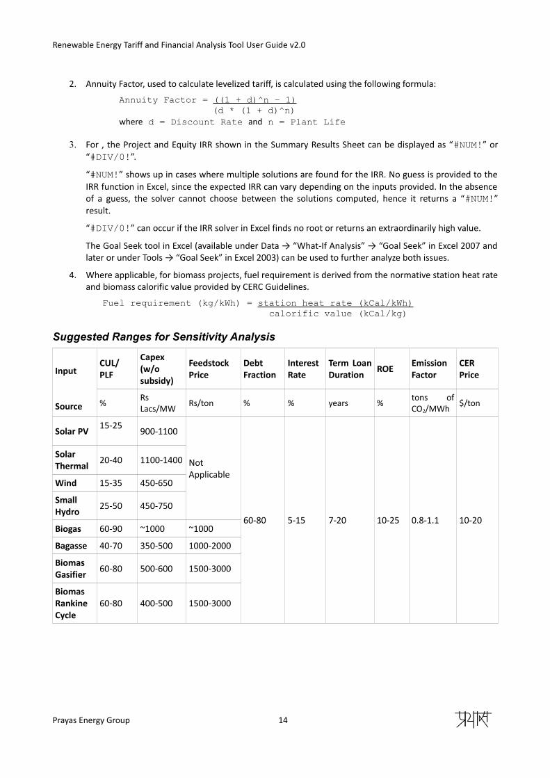
Suggested Ranges for Sensitivity Analysis

Input

Source

CUL/PLF

Capex(w/osubsidy)

FeedstockPrice

DebtFraction

InterestRate

Term LoanDuration ROE Emission

FactorCERPrice

% RsLacs/MW Rs/ton % % years % tons of

CO2/MWh $/ton

Solar PV 15-25 900-1100

NotApplicable

60-80 5-15 7-20 10-25 0.8-1.1 10-20

SolarThermal 20-40 1100-1400

Wind 15-35 450-650

SmallHydro 25-50 450-750

Biogas 60-90 ~1000 ~1000

Bagasse 40-70 350-500 1000-2000

BiomasGasifier 60-80 500-600 1500-3000

BiomasRankineCycle

60-80 400-500 1500-3000



For Off-grid Renewable Energy Projects(These assumptions have been derived from independent project locations a user is free to change theassumptions to suit his/her requirement)

Load Profile

These are a set of assumptions that have been used to determine the load profile for villages. The load profile isfurther used to calculate the required plant size to meet the load. However the load profile can be adjusted byevery user to suit, meet their requirements. The numbers used here as mere assumptions used by thedevelopers to set pace for the further calculations.

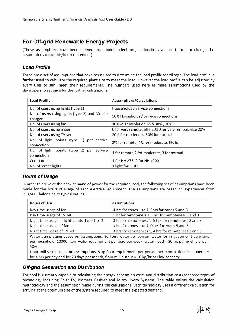
Load Profile Assumptions/Calculations

No. of users using lights (type 1) Households / Service connections No. of users using lights (type 2) and Mobilecharger 50% Households / Service connections

No. of users using fan 10%Solar Insolation >5.5 30% , 10%No. of users using mixer 0 for very remote, else 20%0 for very remote, else 20%No. of users using TV set 20% for moderate, 30% for normalNo. of light points (type 1) per serviceconnection 2% for remote, 4% for moderate, 5% for

No. of light points (type 2) per serviceconnection 1 for remote,2 for moderate, 3 for normal

Computer 1 for HH >75, 2 for HH >200No. of street lights 1 light for 5 HH

Hours of Usage

In order to arrive at the peak demand of power for the required load, the following set of assumptions have beenmade for the hours of usage of each electrical equipment. The assumptions are based on experiences fromvillages belonging to typical setups.

Hours of Use Assumptions

Day time usage of fan 4 hrs for zones 1 to 4, 2hrs for zones 5 and 6 Day time usage of TV set 1 hr for remoteness 1, 2hrs for remoteness 2 and 3 Night time usage of light points (type 1 or 2) 3 hrs for remoteness 1, 5 hrs for remoteness 2 and 3 Night time usage of fan 3 hrs for zones 1 to 4, 0 hrs for zones 5 and 6 Night time usage of TV set 3 hrs for remoteness 1, 4 hrs for remoteness 2 and 3 Water pump sizing based on assumptions: 80 liters water per person, water for irrigation of 1 acre landper household, 10000 liters water requirement per acre per week, water head = 30 m, pump efficiency =50% Flour mill sizing based on assumptions: 5 kg flour requirement per person per month, flour mill operatesfor 4 hrs per day and for 20 days per month, flour mill output = 10 kg/hr per kW capacity

Off-grid Generation and Distribution

The tool is currently capable of calculating the energy generation costs and distribution costs for three types oftechnology including Solar PV, Biomass Gasifier and Micro Hydro Systems. The table enlists the calculationmethodology and the assumption made during the calculations. Each technology uses a different calculation forarriving at the optimum size of the system required to meet the expected demand.



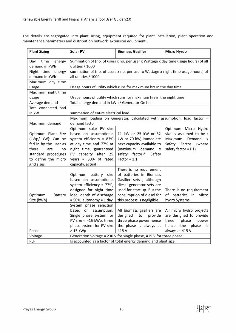
The details are segregated into plant sizing, equipment required for plant installation, plant operation andmaintenance parameters and distribution network extension equipment.

Plant Sizing Solar PV Biomass Gasifier Micro Hyrdo

Day time energydemand in kWh

Summation of (no. of users x no. per user x Wattage x day time usage hours) of allutilities / 1000

Night time energydemand in kWh

summation of (no. of users x no. per user x Wattage x night time usage hours) ofall utilities / 1000

Maximum day timeusage Usage hours of utility which runs for maximum hrs in the day timeMaximum night timeusage Usage hours of utility which runs for maximum hrs in the night timeAverage demand Total energy demand in kWh / Generator On hrsTotal connected loadin kW summation of entire electrical load

Maximum demandMaximum loading on Generator, calculated with assumption: load factor =demand factor

Optimum Plant Size(kWp/ kW): Can befed in by the user asthere are nostandard proceduresto define the microgrid sizes.

Optimum solar PV sizebased on assumptions:system efficiency = 83%at day time and 77% atnight time, guaranteedPV capacity after 25years = 80% of ratedcapacity, actual

11 kW or 25 kW or 32kW or 70 kW, immediatenext capacity available to(maximum demand xsafety factor)* SafetyFactor = 1.1

Optimum Micro Hydrosize is assumed to be :Maximum Demand xSafety Factor (wheresafety factor =1.1)

Optimum BatterySize (kWh)

Optimum battery sizebased on assumptions:system efficiency = 77%,designed for night timeload, depth of discharge= 50%, autonomy = 1 day

There is no requirementof batteries in BiomassGasifier sets , althoughdiesel generator sets areused for start up. But theconsumption of diesel forthis process is negligible.

There is no requirementof batteries in Microhydro Systems.

Phase

System phase selectionbased on assumption:Single phase system forPV size < =15 kWp, threephase system for PV size> 15 kWp

All biomass gasifiers aredesigned to providethree phase power hencethe phase is always at415 V

All micro hydro projectsare designed to providethree phase powerhence the phase isalways at 415 V

Voltage Generation Voltage = 230 V for single phase, 415 V for three phasePLF Is accounted as a factor of total energy demand and plant size



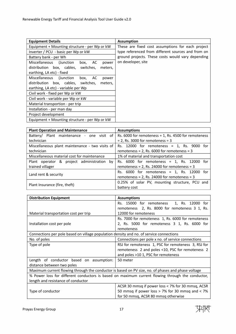
Equipment Details AssumptionEquipment + Mounting structure - per Wp or kW These are fixed cost assumptions for each project

type referenced from different sources and from onground projects. These costs would vary dependingon developer, site

Inverter / PCU - basic per Wp or kWBattery bank - per WhMiscellaneous (Junction box, AC powerdistribution box, cables, switches, meters,earthing, LA etc) - fixed Miscellaneous (Junction box, AC powerdistribution box, cables, switches, meters,earthing, LA etc) - variable per Wp Civil work - fixed per Wp or kWCivil work - variable per Wp or kWMaterial transportion - per trip Installation - per man dayProject development Equipment + Mounting structure - per Wp or kW

Plant Operation and Maintenance AssumptionsBattery/ Plant maintenance - one visit oftechnician

Rs. 6000 for remoteness = 1, Rs. 4500 for remoteness= 2, Rs. 3000 for remoteness = 3

Miscellaneous plant maintenance - two visits oftechnician

Rs. 12000 for remoteness = 1, Rs. 9000 forremoteness = 2, Rs. 6000 for remoteness = 3

Miscellaneous material cost for maintenance 1% of material and transportation cost Plant operator & project administration bytrained villager

Rs. 6000 for remoteness = 1, Rs. 12000 forremoteness = 2, Rs. 24000 for remoteness = 3

Land rent & security Rs. 6000 for remoteness = 1, Rs. 12000 forremoteness = 2, Rs. 24000 for remoteness = 3

Plant Insurance (fire, theft) 0.25% of solar PV, mounting structure, PCU andbattery cost

Distribution Equipment Assumptions

Material transportation cost per trip

Rs. 15000 for remoteness 1, Rs. 12000 forremoteness 2, Rs. 8000 for remoteness 3 1, Rs.12000 for remoteness

Installation cost per pole Rs. 7000 for remoteness 1, Rs. 6000 for remoteness2, Rs. 5000 for remoteness 3 1, Rs. 6000 forremoteness

Connections per pole based on village population density and no. of service connections No. of poles Connections per pole x no. of service connections Type of pole RSJ for remoteness 1, PSC for remoteness 3, RSJ for

remoteness 2 and poles <10, PSC for remoteness 2and poles >10 1, PSC for remoteness

Length of conductor based on assumption:distance between two poles

50 meter

Maximum current flowing through the conductor is based on PV size, no. of phases and phase voltage % Power loss for different conductors is based on maximum current flowing through the conductor,length and resistance of conductor

Type of conductor ACSR 30 mmsq if power loss < 7% for 30 mmsq, ACSR50 mmsq if power loss > 7% for 30 mmsq and < 7%for 50 mmsq, ACSR 80 mmsq otherwise



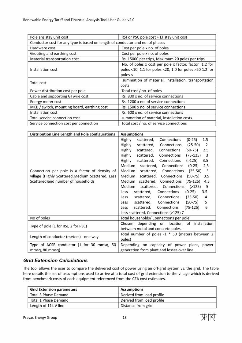
Pole ans stay unit cost RSJ or PSC pole cost + LT stay unit cost Conductor cost for any type is based on length of conductor and no. of phases Hardware cost Cost per pole x no. of polesGrouting and earthing cost Cost per pole x no. of polesMaterial transportation cost Rs. 15000 per trips, Maximum 20 poles per trips

Installation cost No. of poles x cost per pole x factor, factor 1.2 forpoles <10, 1.1 for poles <20, 1.0 for poles >20 1.2 forpoles <

Total cost summation of material, installation, transportationcosts

Power distribution cost per pole Total cost / no. of poles Cable and supporting GI wire cost Rs. 800 x no. of service connectionsEnergy meter cost Rs. 1200 x no. of service connectionsMCB / switch, mounting board, earthing cost Rs. 1500 x no. of service connectionsInstallation cost Rs. 600 x no. of service connections Total service connection cost summation of material, installation costs Service connection cost per connection Total cost / no. of service connections

Distribution Line Length and Pole configurations Assumptions

Connection per pole is a factor of density ofvillage (Highly Scattered,Medium Scattered, LessScattered)and number of households

Highly scattered, Connections (0-25) 1.5 Highly scattered, Connections (25-50) 2 Highly scattered, Connections (50-75) 2.5 Highly scattered, Connections (75-125) 3 Highly scattered, Connections (>125) 3.5 Medium scattered, Connections (0-25) 2.5 Medium scattered, Connections (25-50) 3 Medium scattered, Connections (50-75) 3.5 Medium scattered, Connections (75-125) 4.5 Medium scattered, Connections (>125) 5 Less scattered, Connections (0-25) 3.5 Less scattered, Connections (25-50) 4 Less scattered, Connections (50-75) 5 Less scattered, Connections (75-125) 6 Less scattered, Connections (>125) 7

No of poles Total households/ Connections per pole

Type of pole (1 for RSJ, 2 for PSC) Chosen depending on location of installationbetween metal and concrete poles.

Length of conductor (meters) - one way Total number of poles -1 * 50 (meters between 2poles)

Type of ACSR conductor (1 for 30 mmsq, 50mmsq, 80 mmsq)

Depending on capacity of power plant, powergeneration from plant and losses over line.

Grid Extension Calculations

The tool allows the user to compare the delivered cost of power using an off-grid system vs. the grid. The tablehere details the set of assumptions used to arrive at a total cost of grid extension to the village which is derivedfrom benchmark costs of each equipment referenced from the CEA cost estimates.

Grid Extension parameters AssumptionsTotal 3 Phase Demand Derived from load profileTotal 1 Phase Demand Derived from load profileLength of 11k V line Distance from grid



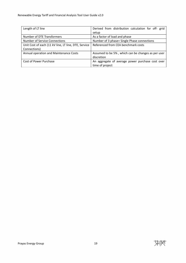
Length of LT line Derived from distribution calculation for off- gridsetup

Number of DTE Transformers As a factor of load and phaseNumber of Service Connections Number of 3 phase+ Single Phase connectionsUnit Cost of each (11 kV line, LT line, DTE, ServiceConnections)

Referenced from CEA benchmark costs

Annual operation and Maintenance Costs Assumed to be 5% , which can be changes as per userdiscretion

Cost of Power Purchase An aggregate of average power purchase cost overtime of project



Known IssuesAlthough reasonable checks are in place, the tool has not been tested to ensure that it works error-free whenextreme values are input. Following issue is known at the time of release of this version.

1. Accelerated depreciation (AD) calculations in the tool don't match CERC's calculations. We areinvestigating this.

Future Enhancements1. Better help text for guidance in entering the input data.

2. Formulation of the financial model used in the tool.

Additional features may be implemented based on feedback received for the current version of the tool.

The spreadsheet and macros have been protected in order to prevent inadvertent changes that can cause thetool to become unusable. If anyone is interested in the unprotected version of the tool, they can contact thedevelopers at the email address provided below.

This Renewable Energy Tariff tool was developed by Prayas Energy Group, Pune. Any questions can be directed [email protected] or to +(91) 20-25420720/65205726 Monday-Friday 10:00am – 6pm.


mailto:[email protected]

Documents

Renewable Energy Tariff and Financial Analysis Tool