Renormalization group analysis of relaxational dynamics in ...theorphys.elte.hu/tel/pdf_pub/ZPB36.pdf · Renormalization Group Analysis of Relaxational Dynamics in Systems with Many-Component

Z. Physik B 36, 343- 355 (1980) Zeitschrift for Physik B © by Springer-Verlag 1980

Renormalization Group Analysis of Relaxational Dynamics in Systems with Many-Component Order-Parameter I*

P. Sz6pfalusy 1 , , and T. T61 z

1 Fachrichtung Theoretische Physik, Universit~it des Saarlandes, Saarbriicken, Federal Republic of Germany 2 Institute for Theoretical Physics, E6tv6s University, Budapest, Hungary

Received September 20, 1979

General properties of the dynamic renormalization group transformation are studied by investigating the multicomponent relaxational model both with conserved and non- conserved order parameter in the large n limit. Exact expressions are given for the transformation of an infinite number of parameters. The strong dependence of all the dynamic quantities on whether the order parameter is conserved or not is illustrated. Critical points of higher order inherent in the model are also discussed. Explicit expressions for the action near the stable fixed points are derived. Different formulations of the dynamic renormalization group are compared and the conditions under which they are equivalent are found.

I. Introduction

The large-n limit of the Landau-Wilson model (n being the number of components of the order parameter) has proved to be an excellent tool for studying how the renormalization group transformation works in describing static critical behaviour [1-6]. Similarly its simplest time-dependent generalization, the large- n system with purely relaxational dynamics is expected to provide a convenient model for testing and expanding various general ideas related to the dynamic renormalisation group (DRG). Although the dynamics of multicomponent systems has been discussed by several authors (see [7] and references therein) and the dynamic critical exponent has been determined up to order 1/n in the relaxational model [8, 9], an analysis using a Wilson type dynamic renormalisation group transformation in the large-n limit with successive elimination of short wavelength fluctuations has been carried out only recently [10, 11]. The parameter space on which the D R G transformation acts has played a central role in the procedure and turned out to be much

* This work was supported in part by Sonderforschungsbereich 130 "Ferroelektrika" ** On leave from the Central Research Institute for Physics, H-1525 Budapest. P.O.B. 49, Hungary

more complicated in the large-n limit than in the small e (e - 4 - d) case. The aim of the present paper is to generalize these latter investigations in different ways. First we include into the discussion the case of the conserved order parameter as well. In this way it is demonstrated that all the dynamic parameters depend on whether the order parameter is conserved or not. The model is rich enough to exhibit critical points of higher order the properties of which are also discussed.

An other aspect of this work is the comparison of different ways of the D R G calculations, namely the perturbative procedures carried out on the equation of motion [12-14] and alternatively in the path probability distribution expressed by the help of an action 1-15-20] and furthermore a saddle-point method in the latter formalism [10]. The couplings in the action which are local in space and time transform among themselves. The saddle- point method which has been used also in [10] enables us to follow the transformation of these couplings in a global way. On the other hand parameters related to the non-local couplings can be treated only by one of the perturbative methods.

0340-224X/80/0036/0343/$02.60

344 P. Sz6pfalusy and T. T61: Renormalization Group Analysis

The main results are presented below along with the outline of the paper. After a short discussion of the model and of the DRG procedure in the path probability formalism (Sect. II) we turn to the discussion of the non-perturbative treatment (saddle-point method) in Sect. III. The exact transformation is given for the local couplings. Even this restricted part of the parameter space contains an infinite number of static and dynamic parameters. Besides the ordinary critical point, the higher order critical points are also investigated. In each case the deviation of the action from its fixed point at T c turns out to be a product of the non-linear scaling field with the largest exponent and of the corresponding eigenvector of the linearised transformation provided we are close to the fixed point. These scaling fields are purely static ones but the eigenvectors bear the marks of dynamics and depend on whether the order parameter is conserved or not. By means of the perturbative method of Sect. IV the transformations of wavenumber- and frequency-dependent couplings are given. The transformed couplings are not all independent since fluctuation-dissipation theorems relate them. Two different repre- sentations of the parameters are presented; some of the details are relegated to Appendix A. It will be demonstrated that at higher order critical points, at T~, the couplings originally local in space and time remain local after the transformation, too. Comparing the DRG calculations carried out on the path probability and on the equation of motion it is found that they are equivalent only if higher order cumulants of the random coefficients generated in the equation of motion are also taken into consideration (Sect. V). This connection yields an interpretation of all the parameters in the action as different cumulants of the random vertices in the equation of motion. In the symmetry breaking phase the parameter space has to be further enlarged as it is demonstrated in Appendix B.

II. The Model and the DRG Transformation in the Path Probability Formalism

We consider a d-dimensional system of volume V the static behaviour of which is described by the Hamil- tonian 1-2, 3]

= d + u ( @ ) ) , (2.1)

where

(VqS)2:½ ~ (V~b,)2, q~2:½ ~ q~2. (2.2) j= l . j = l

qS= {~bjlj= 1,.. . , n} denotes the n-component order parameter with wave number cut-off A. The function U is represented by a Taylor series as

oo

U(q~2) =m__~l= /'/2 m,2m2 (2 q52) m, (2.3)

where the coefficients uz,,, 2 are of order n 1-m to ensure the existence of the limit n--+ oo. The time variation of the order parameter is gov- erned by the following Langevin type equations

6Yg 6j = - L ~ + ~j, j = 1, 2, ..., n. (2.4)

is assumed to be a random field with a Gaussian distribution and white spectrum. The bare coefficient L is constant for a non-conserved order parameter and is proportional to the Laplacian for a conserved one (models A and B in [7, 8]): L = F ( i V ) c, c = 0 or 2. (2.5)

The stochastic process (2.4) can be described equiva- lently by the path probability functional P{~b} which reads

j=1

where ~ stands for the response field [21]. d{q~, ~b} denotes the action [16-19]. In our case

d{~,~} =SdtS ddx i (-~)2L~)j÷i4)2 (()j-aLA dfj) j=1

+ i ~)j Ld~j U(a)(~b 2) ÷ 1/2 rK(e) u(~(~2)) (2.6)

with A

K ( c ) = K a S q~+d-, dq, (2.7) 0

Kd = 21 - a re- d/2/F(d/2). (2.8)

Furthermore we introduced above the following no- tation

U(° (q52 ) =- d ~ u (~z)/d(dp2) i. (2.9)

The last term of d stems from the functional Ja- cobian 1-15, 18, 193 in the large-n limit. The D R G transformation R b is defined on the weight functional exp sd by integrating over shells in the space of wave numbers [17, 20]. The new action is determined by the equation

exp d'{6', 4'}

=S l~ dOj, k,~d4j, k,o~ exp sd{6, qS} (2.10) j , A / b < k < A , ro

P. Sz~pfalusy and T. T61: Renormalization Group Analysis 345

with the rescaled quantities

x,=b-lx , t'=b-zt,

qS'(x', t ' )=b -1 +,/2 +a/2 qS(x, t),

6'(x', t ' )= b-Y qS(x, t). (2.11)

In (2.10) q~j,k,~ and q~j,k,~ denote the Fourier components of the response field and of the order parameter respectively:

4j(x, t)= V -1/2 ~ ~bj, k,o,e i(k~-°'°, (2.12) k,(.O

and similarly for ~a(x, t). Here

~dco (2.13) 2-=Z k ,o ) k < A - -oo

This procedure shows a strong analogy to the static RG [22, 2].

III. Non-Perturbative Treatment (Saddle-Point Method)

The Parameter Space

Before carrying out the calculation we outline the structure of the parameter space. The form of the action we have started with, (2.6), turns out to be not sufficiently general i.e. after the RG transformation new terms arise. It can be proved that the parameters of the functional

ag{(a,(O}=Sdtyddx {--(ojL(oj J

+ i~)j(Oj-aLA qSj)} + Y(~b 2, (p)], (3.1)

(p=i ~ ()jLdpj+(n/2)FK(c) (3.2) j = l

span the whole parameter space involved (at least above T~) provided we treat only local couplings in space and time*. The latter restriction is necessary in order that the saddle-point method be applic- able. Y is represented by a double Taylor series

Y(~bz, cp)= ~ ~, UE,,,,,2t(p'(2~b2) ~- ' (3.3) m = l l < l < m

w i t h u2m, 2t=(9(n l-m) for all/'s. Initially

* These couplings transform among themselves in the large n limit. Some of the couplings treated here are related to frequency dependent ones as will be seen in the next Section

Y(q52, cp) = ¢p U(a)(q52) (3.4)

as it follows from (2.6). For l= 1 the couplings in (3.3) agree with those in (2.3). For the sake of convenience we introduce the no- tation for the derivatives of Y as follows

y~, j(q~ 2, q0)= 0 i+j Y(q52, ~o)/~3(q52) i 0p j. (3.5)

Y(q52,0) can be proved to be a constant after the transformation which will not be regarded as a parameter*. Thus YO, l(q52, (p) will be of importance since it specifies all the parameters besides a and F. Therefore we can specify the parameter space as

/* = (a, F, Yo, ~(~ b2, (P))

o r

/~ = (a, 1", {u2,,,2,lm>=l>= 1}). (3.6)

The static parameters given by (2.1) and (2.3)

#st = (a, {u2m, 21m=> 1}) (3.6a)

form of course an invariant subset in the parameter space. Finally we note the relationship

Y~, ~(q52, 0) = U (i+ ~)(~b2). (3.7)

The Transformation and Fixed Points

The D R G transformation can be performed exactly in the large-n limit. The calculation goes on the same lines as in [10] where only the case of a non-conserved order parameter was treated, therefore we mention only the main steps of it. The integral in (2.10) over ~j,k,~ is straightforward since d is quad- ratic in this variable. In carrying out the integral over qSk,~'s the saddle-point method turns out to be applic- able. For the first two parameters we obtain

a'=b-~a, F'=b-2+~-C+ZF (3.8)

indicating that a finite fixed point can be achieved only if

~]=0, z = 2 + c (3.9)

which are well-known results of previous works [2, 8, 9]. The transformation of the function Yo, l(q 52, qo) cou- ples to that of Yl,o(q52, ~o). For d > 2 it is found, using the definition (2.9), that

* This is why the sum over 1 in (3.3) starts with l= 1


]7' b 2 o,~(¢2, ~0)= U°)(bZ-aQ(¢ 2, qo)+N~), (3.10)

y' b 4-a 1,0(¢2, @) = U(2)(b2-dQ(¢2,~p)+N~)R(¢2, cp), (3.11)

where ¢2 and qo denote the rescaled fields, furthermore

> Q(¢2, (p)=¢2_Nc+(n/2) ~ (q~/2S-1 _q-2) , (3.12)

q

R(q5 2, ~o)= q~ - (n/2) S (q3c/Z(q2 + y~, 1(¢2, (p)) S-1 _qC)

q (3.13) with

S-{qC(q2+ y~,,(¢2, tp))2-2Y~,o(¢2,~o)} t/2. (3.14)

The constant N c is given by

N~ = (n/2) K d A d- 2/(d - 2) (3.15)

and

A b

i ==-Ka ~ dqq a-l" (3.16) q A

Since a and F do not transform they have been set equal to unity. In the special case of c = 0 Eq. (3.10)-(3.14) go over to the corresponding ones in [10]*. An important feature of Eq. (3.10)-(3.15) is that at (p = 0 they describe the transformation of the static parameters. In fact for Y~,1(¢ 2, O)=t ' (¢ 2) we recover the expression first obtained by Ma (see (4, 35) in [23). This is a consequence of the fact that Y~,o(¢2,0)-0 as it follows from (3.11). The right hand sides of (3.10) and (3.11) can be expanded as

1/;,' !) o,~(@,~0)=b ~ ~ (1/j V~+~(NO j=o

• b(2-a)J[Q(¢ 2, q))]J, (3.17)

y , t ~ 2 ~,o,~" , q°) =bS-e ~ (l/j!) u(J+2)(Nc) j - O

• b(2-d)J [Q(¢ 2, ~o)]J R(¢ 2, cp). (3.18)

The fixed point is generated by taking the limit b-+ oQ. It can be seen from these equations that a necessary condition for the existence of a finite fixed point is

* Note that there are differences in the notations: t(~z), v(052), y(SZ, q~) and X(~2,~o) of [10] are here Um(4~z), U(2)(052), Y~;, 1(05 2, ~o) and 2 Y;, o(q52, ~o) respectively. Furthermore it can easily be seen that b2-dQ + N~= b 2-e 02+ ~, where t~ is defined by (21) of [10] for c=O

U(1)(Nc) = 0 (3.19)

which specifies the critical surface in the parameter space. This is, of course, a well-known condition from statics [23. For d > 4 the Gaussian fixed point is reached

Yff(¢2, ~o)-0.

Here and the following the fixed point values of the quantities are marked by an asterisk. Below four dimensions let us discuss first the case when u(E)(Nc)>0. Then it follows from (3.17) and (3.18) that Y0,1 and Y~,o can approach finite fixed point expressions only if Q and R tend to zero in the limit b - * ~ . Using (3.12) and (3.13) the fixed functions Y0*,t and Y~ 0 are given by the coupled integral equations:

02 =Nc- (n /2 )K d ~ (qC/2(S*)-I _q-2)qe-1 dq, (3.20) A

cp=(n/2) K a ~ (q3c/e(q2 + E* o, 1(¢2~o)) A

. ( S , ) - 1 _q~) qa-1 dq (3.21)

with

S*-{q~(q2+ y~,~(42,~o))2-2Y~,o(¢e, cp)}l/z. (3.22)

The fixed point expression of the action is given by the general relationship

q~

y(¢2, (p)= S Yo, 1(¢ 2, q~) do. (3.23) 0

The transformation of the function Yo, 1(¢ 2, (#) specifies, at least in principle, the transformations and fixed point values of all the parameters u2,,,2> It is more convenient however to consider the different derivatives of Y taken at ¢2 = N c and ~o=0 as an other set of parameters. The fixed point values of some of these quantities are listed below:

(1/2) Y~ l(Nc, 0)= AS-a(4 -d) (nKa)- 1,

(1/2) Y~2(N~, O) = A 2 -¢-d (4 - d ) 2 (6 + c - d ) - i (n K d ) - 1,

(1/8) Yz*, I(N~, 0)

= A6- 2d(4 - d ) 3 (6 - d ) - 1 (nKd)- 2,

(1/4) Y~2(N~, O)

=A4_c_2d (4-d)3 ~ 4 ( 4 - d) 3 } (nKd) 2 [ ( 6 + c - ~ - d ) 8 + c - d '

(1/6) go*, 3(No, o)

P. Sz6pfaIusy and T. T61: Renormalization Group Analysis 347

=A2_2c_2a 2(4-d) 3 )" 2 (4-d) 2 (nKa) 2 [ ( 6 + c - d ) 2 ( 6 - d )

3(4-d) 1 } (3.24) ( 8 + c - d ) ( 6 + c - d ) ~ l O + 2 c - d '

Yj*o(Nc, 0) = 0, j = 1,2, ....

These formulae illustrate the strong dependence of the dynamic quantities on whether the order parameter is conserved or not.

Higher Order Critical Points

obtained by taking first the limit b ~ oo. and sub- sequently the limit n ~ oo. Such a procedure could account for the features of the exact solution of the model for equilibrium properties [25] according to which there exists a tricritical point in three dimensions without, however, logarithmic corrections to the mean field behaviour. This possibility is also in accordance with the results by Stephen et al. [30], who pointed out that the critical region (in which the logarithmic corrections arise) shrinks to zero when n--+ oo in three dimensions at the tricritical point. It is expected that similar situation occurs in case of the critical point of o "th order at d, = 2 ~/(a - 1).

Under special conditions we can arrive at fixed points describing higher order critical points (see for a discussion of higher order critical points [23]). Name- ly for

U(J)(N~)=O, 1 < j < a

and

U(~)(Nc) > 0, o-= 3, 4 . . . . (3.25)

and for d > 2 a / ( ¢ - l ) the recursion relations (3.17), (3.18) lead to the Gaussian fixed point, which in this case specifies a critical point of order o. (The ordinary critical point for d >4 would corresponds to o- =2). Note that Q(N~,O)=R(Nc, O)=O, which ensures that for l < j < o - U'(J)(N¢) - Y]_ I, I (Nc, 0) are also zero if (3.25) is fulfilled. Let us discuss first the tricritical point, many of the static properties of which have been studied by several authors for large n [4, 5, 24-29]. The recursion relations (3.17) and (3.18) do not lead to a finite fixed point below three dimensions corresponding to a tricritical point*. It is in accordance with the results of Emery [25] who has found that for d<3 the critical line terminates at a critical end point and a first order phase transition takes place when decreas- ing U(2)(Nc) already for small positive values of it. There is no finite fixed point of the recursions (3.17) and (3.18) at d = 3 either.* This feature can be contrasted with the behaviour of the recursions at d = 4 where the Gaussian fixed point is reached in the limit b-+ oo. The reason behind this is that Q and R have contributions proportional to In b at d = 4, while they develop no logarithmic singularities at d = 3 even when the condition of tricriticality (U(2)(N¢)=0) is fulfilled. It is expected, however, that such logarithms show up when calculating to order 1/n. Then a fixed point describing tricritical behaviour at d = 3 may be

* These statements hold also, if we consider the recursion relations at cp = 0, which corresponds to statics

The Large-b Behaviour of the Transformation

The properties of the transformation near the fixed points can be deduced from (3.10), (3.11). It is found that for 2 < d < 4 at T~ in leading order in b

Y;, l(e 2, e ) - go~ 1(4 2, ¢o) = be- ~ g a(Yd~ 1 Y~ o)/a (P, (3.26)

Y;, o (~b 2, (p)- Y~0(¢ 2, cp)

= b a- 4 g (?(y~,, Yi*, o)/0(¢2), (3.27)

where

g = [I11", 1(No, 0)] -~ - [I11, ~(Ne, 0)] - 1 (3.28)

and Y~ 1(No, 0) is given by (3.24). Then it follows from (3.23) and (3.26) that for large b

y,(q~2, cp)- y , ((~2, ~0)

=ba-4g ro*, 1 (~b 2, ¢o) r~*. o(¢ 2, ¢o). (3.29)

It should be emphasized that the expressions (3.26), (3.27) and (3.29) are not restricted to such starting points in the parameter space which lie near the fixed point. As a matter of fact due to the special form of the initial action (2.6) the starting point could not generally be choosen in the vicinity of the fixed point. It can be shown that g is a non-linear scaling field*, which transforms at T~ as g'=g b a-4. It is interesting to point out t h a t Yo*i(• 2, (p) Yt*o(~ 2, (p) is an eigen- operator of the linearised transformation around the non-trivial fixed point.

* The scaling field g is of purely static character (i.e. it is a combination of static parameters only, as can be seen from (3.28) and (3.7), and agrees with what has been determined in the RG analysis of the statics of the model [4, 5]. The complete hierarchy of the scaling fields including the dynamic ones will be given in a subsequent paper [31]

348

Similarly we can investigate the transformation in the neighbourhood of the trivial fixed point in the case of higher order critical points. We obtain for a ath order critical point for large b

y,((~2, @) : b2+(2 -d)(a- 1)(1/(Or _ 1)!)

• U(¢)(Nc)(~b 2 - N y -1 ~p (3.30)

provided d is larger than de. It turns out that the non-linear scaling field with the largest exponent in this case is proportional to U(¢)(N~) at T~ (and the exponent is 2+ (2 -d ) (~ r -1 ) ) . Moreover (~b2-Nc)¢-lcp is just the corresponding eigenvector of the linearised transformation. The fact that the deviation of the action from its fixed point expression for large b at T~ is the product of the non-linear scaling field with the largest exponent and the corresponding eigenvector of the linearised transformation is expected to be valid for all cases when there is only one non-linear scaling field at T¢ which belongs to the largest exponent•

IV. Perturbative Method in the Path Probability Formalism

The multiple integral (2.10) can be evaluated per- turbationally as well [17, 20]. In order to do this we decompose the action into a harmonic part and the interaction

P. Sz6pfalusy and T. T61: Renormalization Group Analysis

dr{~), ~)}=S dt y ddx ~ {u4,2i~jL~)j2~ )2 j=l

+u4,2FK(c) q~2 +.. .}. (4.1)

The only non-vanishing averages over the harmonic part are given in terms of Fourier components (2.12) as

- i FkC(4)j ,k , ~, ~j , -k , - ,o) o ~ G(°)( k, co) = FkC(-ie)+ FkC(ake +u2,2)) -1, (4.2)

( O j, k,~, ~ j, -~, - ~ 5 o ~ C(°~( k, co)

= (2/co) Im G(°)(k, o3), (4.3)

where G (°) denotes the free response function and C (°) is the corresponding correlation function. To represent the contributions to the integral

S H dJpj, k,~dOj, k,,oexpd o ~ d]/l! (4.4) j ,A/b<k<A,w l=0

it is convenient to introduce diagrams. In the large-n limit only graphs with a maximal number of closed loops survive because every loop involves a factor n. The topological structure of these diagrams corre- spond to that of the static ones [3]. Figure 1 shows some of the diagrams coming from the l= 3 term of (4.4). Looking at the graphs one concludes that only those vertices give contributions in which both legs belong-

G ° . • ° O • ° • ° iU 6.2

© ©

©

V iU4.2

Fig. 1. Some diagrams in the DRG calculation of the large-n limit. Notations:

V :U4.2

C(°)(k, c~), G(°)(k, co). External legs: qbzk, o , with k<A/b. Internal lines carry momenta between A/b and A

P. Sz6pfalusy and T. T6I: Renormalization Group Analysis 349

ing to one endpoint carry either large or small momenta. If in addition the k- and co-dependent parts of the diagrams are not considered the net wavenumber and frequency transfers of the potential lines are zero. As a matter of fact, in the language of diagrams this argument justifies the approximations done when performing the D R G transformation by the non- perturbative method (see Eqs. (11) and (13) in [10]). The steps of the calculation can be summerised in the following• Infinite subsets of graphs are summed up by using self consistently dressed correlation and response functions and an effective interaction, containing the series of bubble graphs*. After introducing new scales corresponding to (2.11), choosing )? as ~ / 2 - 1 - d/2 in order to ensure a finite coefficient of the term i q~'~' and making use of the linked cluster theorem we arrive at a new action containing couplings non-local in space and time. Let

U2m, 2/(kl, "'" km- 1 ; COl, "'" com 1) (4.5)

denote the coupling described by a graph with 1 external wavy lines and 2 m - 1 external straight lines. We can write

]A=(a, I', {U2m, 21(kl, ... kin_l; col, ... (J)m-t) jm>l> 1}) (4.6)

indicating that all parameters of the functions U2rn, 2/

(for instance the Taylor coefficients) are to be considered as elements of the parameter space. It is easy to see that graphs containing K(c) (the contribution of the Jacobian) do not determine new independent parameters**. In the previous treatment this has been reflected in that, that always the combination ~o, (3.2), has been involved. The lack of terms like q~,2, q~, 3 etc. in s¢' has the important consequence that the noise in the equation of motion remains Gaussian (see for the form of the action in case of non-Gaussian noise [19]). This is one of the simplifying features of the dynamics in the large-n limit. The results for the first few couplings U2m ' 2/ are given in Appendix A. Here, instead, we introduce an other representation of the parameters in order to show the connection between the results of the present and previous Sections more directly. Let us define:

U2m, 2/=U2m, 2/-~" ~ bl2(m+d),21 j ] j = l (-}-l~--I](2Nc)J. (4.7)

* The bubbIe graphs here consist of one response and one correlation function ** This feature should be compared with the role of the Jacobian in other types of perturbation expansion [18, 19]

It is worth while mentioning that the linear combination (4,7) has a well-defined meaning in the language of the usual perturbation expansion*. U2m ,2/ is a sum of vertices of the same type (i.e. with 2m external lines, among them 1 response field lines) where the jth term of the series comes from u2(m+;) ' 2l but j pair of the order parameter lines are closed to form fully dressed Hartree loops of the correlation function (whose contribution gives the average value of q52) evaluated at T~. The correlation function in this formalism is given by (4.2), (4.3) but with U2, 2 instead of 122, 2, Since Uz, z=U(1)(Nc) it is zero at T~ (see (3.19)), and the contribution of a Hartree loop turns out to be simply the constant N c, (3.15), which has frequently occured in our calculation previously. The self-loop of the response function, on the other hand, cancels the contribution of the Jacobian as required by causality [-18, 19]. In other words this means that the average of ~0 vanishes and this is why a summation over the second indices of u is not involved in (4.7). Figure 2 shows as an example how U¢, 2 can be represented by diagrams. New vertices similar in spirit to those defined above have been used in calculating static and dynamic critical indices at critical points of higher order just below the critical dimensionality do (see [32, 33]). When performing the D R G transformation we start with the new parameters U2m,21 and find that the corresponding transformed quantities become k- and co-dependent, U;,,,, 2/(kl . . . . k,,_ 1 ; col, .., co~- 0, where k 1 . . . . and co,,.. , denote the rescaled wavenumbers and frequencies, respectively. For U~, 2 (k, co) one obtains

U~, 2(k, co)= 1 + b4-~(n/2) V(2)(I~ ~)) Ib~2)(k, co)' (4.8)

where U (2) is defined by (2.9) and I~l)=b2-dQ(N~,O) + N c with Q as given by (3.12) and

= ~ ( q 2 + U ; , 2 ) - l ( ( k - q ) 2 + U ; , 2 ) - i A <q <Ab, A <lk-q] <Ab

qC(q2+U;,2)+(k-q)~((k-q)2+U£,2) - i co + qC(q2 + U£,2) + (k-q)~ ( (k-q)2 + U;,2) d d q

• (2 rO d. (4.9)

Here a and F have been set equal to unity and U£,2 can easily be deduced from (3.10) as

** As contrasted to the RG calculation, here the momenta of the internal lines are not restricted to a shell but run from zero to the cut-off

350 P. Sz6pfalusy and T. T~I: Renormalization Group Analysis

0 0 O 0 + ) - - i u - : { + + ..-

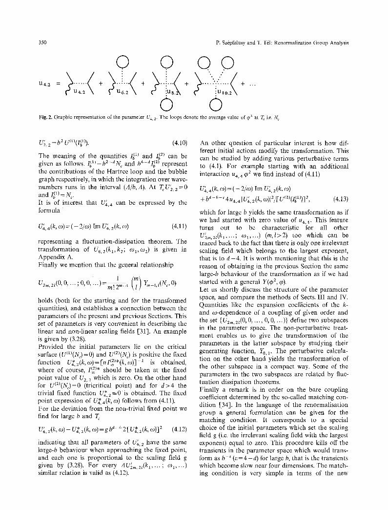
0 0 Fig. 2. Graphic representation of the parameter U< 2. The loops denote the average value of ~b 2 a t T~ i.e. N~

U2, 2 = b 2 Uo)(I~I)). (4.10)

The meaning of the quantities Ib (1) and Ib ~2) can be given as follows. I~)-b2-dNc and b'*-aI~ 2) represent the contributions of the Hartree loop and the bubble graph respectively, in which the integration over wavenumbers runs in the interval (A/b, A). At T~ U~, 2 =0 and I~l)= N~. It is of interest that U~, 4 can be expressed by the formula

U~, 4(k, co) = ( - 2/co) Im U~,i(k, co) (4.11)

representing a fluctuation-dissipation theorem. The transformation of U6,2(kl, k2; c01,co2) is given in Appendix A. Finally we mention that the general relationship

Uzm ' 2t(0, 0,... ; 0, 0, " " ) = m! 2 m-t

h o l d s (both for the starting and for the transformed ctuantities), and establishes a connection between the parameters of the present and previous Sections. This set of parameters is very convenient in describing the linear and non-linear scaling fields [31]. An example is given by (3.28). Provided the initial parameters lie on the critical surface (g(1)(Nc)=O) and U(2)(Nc) is positive the fixed function U* z(k, co) = [nI~)*(k, co)]- 1 is obtained, 4, where of course, I~ )* should be taken at the fixed point value of Ue, e which is zero. On the other hand for u(Z)(Nc)=0 (tricritical point) and for d > 4 the trivial fixed function U~e-=0 is obtained. The fixed point expression of U* 4(k, co) follows from (4.11). For the deviation from the non-trivial fixed point we find for large b and T~

U~,2(k, co)-U*,2(k, oJ)=gba-¢2[U*2(k, co)] 2 (4.12)

indicating that all parameters of U~, z have the same large-b behaviour when approaching the fixed point, and each one is proportional to the scaling field g given by (3.28). For every AU;,n,21(k>... ; col,...) similar relation is valid as (4.12).

An other question of particular interest is how different initial actions modify the transformation. This can be studied by adding various perturbative terms to (4.1). For example starting with an additional interaction u<4 q~2 we find instead of (4.11)

U•, 4(k, co) = ( - 2/co) Im U4, i(k, co) +ba-6-C4u4,41U~,2(k, co)12/[U(2)(I(bl))] 2, (4.13)

which for large b yields the same transformation as if we had started with zero value of u¢,4. This feature turns out to be characteristic for all other U~m, 21(kl . . . . ; col .. . . ) (re, l>2) too which can be traced back to the fact that there is only one irrelevant scaling field which belongs to the largest exponent, that is to d - 4 . It is worth mentioning that this is the reason of obtaining in the previous Section the same large-b behaviour of the transformation as if we had started with a general Y(~b 2, ~o). Let us shortly discuss the structure of the parameter space, and compare the methods of Sects. III and IV. Quantities like the expansion coefficients of the k- and co-dependence of a coupling of given order and the set {Uzm,2~(0, 0 . . . . ,0, 0, ...)} define two subspaces in the parameter space. The non-perturbative treatment enables us to give the transformation of the parameters in the latter subspace by studying their generating function, Yo, 1. The perturbative calculation on the other hand yields the transformation of the other subspace in a compact way. Some of the parameters in the two subspaces are related by fluctuation dissipation theorems. Finally a remark is in order on the bare coupling coefficient determined by the so-called matching condition [34]. In the language of the renormalisation group a general formulation can be given for the matching condition. It corresponds to a special choice of the initial parameters which set the scaling field g (i.e. the irrelevant scaling field with the largest exponent) equal to zero. This procedure kills off the transients in the parameter space which would transform as b -~ (~- 4 - d) for large b, that is the transients which become slow near four dimensions. The matching condition is very simple in terms of the new

P. Sz6pfalusy and T. T61: Renormalization Group Analysis 351

parameter U4, 2 since the requirement g = 0 can be fulfilled only if

U4,2 = U* 2(0, O)

as can be seen from (3.28). In the special case when we start with the usual 4)4 model e.g. with

a(4) 2) =/g2, 2 4)2 ..~//4, 2 (4)2) 2 (4.14)

we have u~, 2 = U4, 2, and thus the matching condition requires a special bare coupling constant u4, 2c as

u4, 2c= U*,2(0, 0).

It is worth while comparing u4, 2c with the fixed point expression of u4,2(0,0) (see (A.2)) for small e. We obtain that they agree up to order ea in accordance with the results of [35], but they differ already in a term of order e3. Closing this Section let us turn to a short discussion of the case of higher order critical points. The corresponding recursions can be read off from the general ones (for example (4.8), (A.5)). At a (r th order critical point (see (3.25)) we find at T~ that

U;,,, 2~(k~ . . . . ; o)1, . . . )=0

for re<a , l < m ,

U2 ,2Z(kl . . . . ; COl, . . . )

=b 2+(2-a)(°- 1)(21 - ~ / ( a - 1)[) U(~)(N~) (Sz, 1 (4.15)

valid for arbitrary b. Furthermore for large b

U;, , ,a(k , . . . . ;o)1,--.) (4.16) =bZ+(2-a)(m-1)(21-m/(m - 1)!) U(")(N~), m > a .

It is apparent that k- and co-dependences do not arise in the couplings at higher order critical points at T~ which is due to the fact that the quantity U~, 2(k, 0)) vanishes at To. A consequence of (4.15) is that at a critical point of order a the scaling field with the largest exponent, 2 + ( 2 - d ) ( a - 1 ) , is just U(~')(N~) as already mentioned at the end of the last Section. Of course for d>d~ the Gaussian fixed point is obtained.

= + ~- / ..... ~ + " "

Fig. 3. Graphic representation of the equation of motion after the first iteration in step a. Notations: - - qSj, k,~, - - ,~(o) ~ j , k, co

=G(°)~j.k,o]FkC, > GW)(k, co), . . . . . (-u4,2). Lines with a slash carry wave numbers larger than A/b

place the variables 4)j,k,~, k < A / b by new ones corresponding to (2.11). Through this procedure we arrive at new equations of motion which are more complicated than the starting ones, they contain higher order couplings and random vertices. The parameter space should contain not only the mean values of these vertices but all higher order cumulants among them [36, 14]. Our model serves as a good example to illustrate this general concept. Let us start with the 4) 4 model, (4.14). Step a) can be performed by an iterative solution of Eq. (2.4). The result of the first iteration is represented in Fig. 3 indicating that the coefficient of 4)y,k,~ on the r.h.s, has become a random variable the full specification of which requires the determination of all its cumulants [14]. As a matter of fact none of these cumulants can be neglected in the large-n limit. An other important difference between our case and a calculation up to order e is that we must not stop after the first iteration as the successive steps generate cumulants of the same order of magnitude as the first one. Fortunately the leading contributions in n can be summed up yielding closed expressions for the cumulants. Figure 4 shows some examples in a graphic representation: azm,2~ denotes the contribution of diagrams with l external response function lines and 2 m - l order parameter lines. Comparing the graphs of the perturbation expansion for the action and those just discussed, one immediately recognizes that their contributions are es- sentially identical. If weighting factors are also taken into consideration the following simple relation is found

V. DRG Transformation Carried out on the Equation of Motion

If the D R G transformation is defined on the equation of motion it involves the following steps [12-14]. a) Eliminate the variables 4)j,k,~o with A / b < k < A by solving their equations of motion in terms of the remaining ones and the random forces and substituting the solutions in the remaining equations, b) Re-

U2m,21(kl . . . . k , , -1 ; 0)1 . . . . COm- O

=lu2m, 21(kl, .--km_a; CO1, ..-C%_ 1)- (5.1)

This relationship indicates that the two definitions of D R G are equivalent only if the higher cumulants of the random vertices in the equation of motion are taken into account as elements of the parameter space. Moreover it provides a physical interpretation of the new couplings generated by the D R G in the action.


_,_z___O___x.,_

r I I I !

J--&---',- ^ A

U4.4 U6.4

I . I

y , v , 0 I I I

l I I

^

U6.6

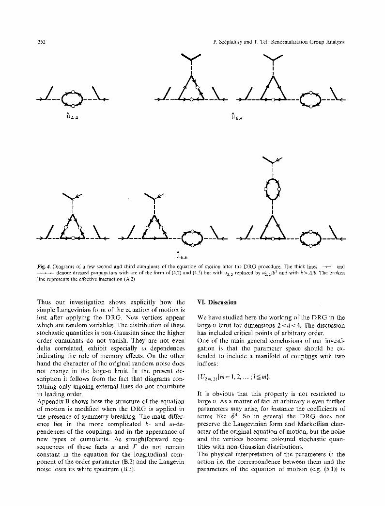
Fig. 4. Diagrams of a few second and third cumulants of the equation of motion after the D R G procedure. The thick lines ~ and , o ~ denote dressed propagators with are of the form of (4.2) and (4.3) but with u2, 2 replaced by u'2,z/b z and with k>A/b. The broken

line represents the effective interaction (A.2)

Thus our investigation shows explicitly how the simple Langevinian form of the equation of motion is lost after applying the DRG. New vertices appear which are random variables. The distribution of these stochastic quantities is non-Gaussian since the higher order cumulants do not vanish. They are not even delta correlated, exhibit especially co dependences indicating the role of memory effects. On the other hand the character of the original random noise does not change in the large-n limit. In the present de- scription it follows from the fact that diagrams containing only ingoing external lines do not contribute in leading order. Appendix B shows how the structure of the equation of motion is modified when the D R G is applied in the presence of symmetry breaking. The main difference lies in the more complicated k- and co-dependences of the couplings and in the appearance of new types of cumulants. As straightforward con- sequences of these facts a and F do not remain constant in the equation for the longitudinal component of the order parameter (B.2) and the Langevin noise loses its white spectrum (B.3).

VI. Discussion

We have studied here the working of the D R G in the large-n limit for dimensions 2 < d < 4 . The discussion has included critical points of arbitrary order. One of the main general conclusions of our investigation is that the parameter space should be ex- tended to include a manifold of couplings with two indices:

{g2m,21jm= 1, 2, . . . ; l < m } .

It is obvious that this property is not restricted to large n. As a matter of fact at arbitrary n even further parameters may arise, for instance the coefficients of terms like q~4. So in general the D R G does not preserve the Langevinian form and Markoffian character of the original equation of motion, but the noise and the vertices become coloured stochastic quantities with non-Gaussian distributions. The physical interpretation of the parameters in the action i.e. the correspondence between them and the parameters of the equation of motion (e.g. (5.1)) is


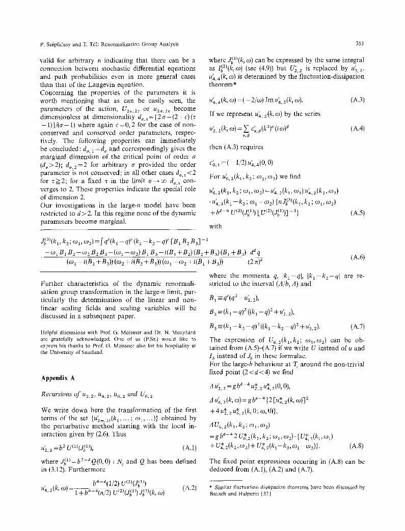
valid for arbitrary n indicating that there can be a connection between stochastic differential equations and path probabilities even i n more general cases than that of the Langevin equation. Concerning the properties of the parameters it is worth mentioning that as can be easily seen, the parameters of the action, U 2 a , 2 ~ o r u 2 a , 2 z become dimensionless at dimensionality d~, ~ = [2 a - (2 + c) (z -1) ] / (a-1) where again c=O, 2 for the case of non- conserved and conserved order parameters, respectively. The following properties can immediately be concluded: do, 1 = d~ and correspondingly gives the marginal dimension of the critical point of order a (d,>2); d~,2=2 for arbitrary o- provided the order parameter is not conserved; in all other cases d~,~ <2 for z>2 ; for a fixed z in the limit a--+ oo d~,~ con- verges to 2. These properties indicate the special role of dimension 2. Our investigations in the large-n model have been restricted to d > 2. In this regime none of the dynamic parameters become marginal.

where Jb(2)(k, 0)) can be expressed by the same integral as Ib(i)(k, 0)) (see (4.9)) but U£, 2 is replaced by u~, 2. u'<4(k, 0)) is determined by the fluctuation-dissipation theorem*

u;, 4(k, 0)) = ( - 2/0)) Im u~,, 2(k, 0)). (A.3)

If we represent u' 2(k, 0)) by the series 4,

/A~, 2 (k, 0)) = ~ c;, ~ (k2) ~ (i 0))P (A.4) a, fl

then (A.3) requires

c{~,1 = ( - 1/2)u~,, 4(0 , 0)

For u6, 2(kl, k 2 ; (01, 0)2) we find

U;, 2(kl,/*;2; 0)1, 0)2) = u~, 2(kl, 0)1) u~, 2 (k2, 0)2)

• U4, 2(kl - k 2 ; 0 )1-0)2) {nJ(b3)(kl, k2; 0)1, 0)2)

+ b a- 6 U(3)(j~I)) [-V(2)(jb{1)) ] - 3} (a .5)

with

Jb(3)(kl, k2 ; 0)i, 0)2) = ~ qC(kl - q)C (kl - k2 - q)~ [B1 B2 B3]-1

-0)1BI B2 -0)2B2 B3 -(0)1-0)2) B1 B3 -i(B1 +B2) (B2 +B3) (Bt +B3) da q (0)1 + i(B1 +B2)) (0)2 + i(B2 +B3)) (0)1-0)2 + i(Bt +B3)) (2 7z) d

Further characteristics of the dynamic renormalisation group transformation in the large-n limit, par- ticularly the determination of the linear and non- linear scaling fields and scaling variables will be discussed in a subsequent paper.

Helpful discussions with Prof. G. Meissner and Dr. N. Menyh•rd are gratefully acknowledged. One of us (P.Sz.) would like to express his thanks to Prof. G. Meissner also for his hospitality at the University of Saarland.

Appendix A

R e c u r s i o n s of U2, 2, hi4., 2, U6, 2 and U6, 2

We write down here the transformation of the first terms of the set {U~m,2t(k 1 . . . . ; 0)1, "")} obtained by the perturbative method starting with the local interaction given by (2.6). Thus

U~, 2 = b e U(1)(J~I)), (A.1)

where d~l)= b 2-d {2(0, 0) + N c and Q has been defined in (3.12). Furthermore

b4-a(1/2) U(2)(J~I)) (A.2) U~, 2(k, 0)) = 1 +b#-a(n/2) U(2)(J~ 1)) J~2)(k, 0))

(A.6)

where the momenta q, Ik l -ql , I k l - k 2 - q ] are restricted to the interval (A/b, A) and

B 1 -=qC(q2+u2,2),

B2 _ (k 1 _ q)2 ((kl _ q)2 + u,2, 2),

B3 ___ (k 1 __ k2 _ q)2 ((kl _ k2 _ q)2 + u~, 2)" (A.7)

The expression of U6,2(kl,k2; col,0)2) can be obtained from (A.5)-(A.7) if we write U instead of u and I b instead of Yb in these formulae. For the large-b behaviour at T~ around the non-trivial fixed point (2 < d < 4) we find

A t l d - 4 U2,2 U4 ' U2,2 = g o * * 2(0,0),

A l,l*4, 2 (k, (I)) = g b d - 4 {2 Eul, 2 ( k, 0))] 2

+ 4u~,2 u~,2(k, O; 0),0)},

A U6, 2(kl, k2; 0)1, 0)2)

=g bd-#2 U~,2(k,, kz; 0)1, 0)2)" { U*, 2(k> 0)0

-F U:, 2(k2, 0)2) + U:. 2(kl - k2, 0)1 - 0)e)}' (A.8)

The fixed point expressions occuring in (A.8) can be deduced from (A.1), (A.2) and (A.7).

* Similar fluctuation dissipation theorems have been discussed by Bausch and Halperin [37]


Appendix B

DRG in the Presence of Symmetry Breaking in Case of a Non-Conserved Order Parameter

In the presence of a homogeneous time-independent external field H coupled to the first component of the order parameter the average of q~ becomes non-zero, (~bl(x, t ) )=M(H). According to the equation of state [3] M=(9(na/2). In order to study quantities of the same order of magnitude in the equation of motion it is convenient to separate the contribution of M by substituting

ff) l , k ,w - M (H) V 1/2 (~k, o 2 7r c5(0))--* q51,k, o,,

which yields different equations of motion for the longitudinal component (j = 1) and for the transverse ones (j > 2). In both cases vertices with an even power of q5 are also involved. After applying the DRG a number of new dynamic parameters arise, not necessarily independent ones. We recall here only a few of them for the case when we start from the q~* model (4.14). The transverse parameters u~, 2 T, a), F~ are given by similar transformations as (A.1) with U(1)(X)=U2,2T+U4,22X and (3.8). Initially U2,2T=U2,2+U4,2 M2. If a T and F r are chosen to be unity u'4, 2r(k, co) is determined by (A.2) but u~, 2 is to be replaced by U2,2T. An interesting novel feature of the transformation is the k- and 0)- dependence of the averaged longitudinal two-leg vertex (see Fig. 5 a)

u'z,2L(k, 0))=U'2,2T + 2U'4,2T(k, 0 ) )M ' z (B.1)

where

M' = b d/2 - a M.

The latter relation indicates that M = 0 is required on the critical surface. As a consequence of (B.1) neither ak nor F L' remains unchanged by the D R G transformation

' a+aU'2'2L(k'O) k=o' a L = ~k 2

1 _ 1 au~,2L(O,?) . (B.2) r + a ( - i 0 ) ) ,o=o

© > O_ _ _ Q ~ _ _ _Q___ >

a)

,. C)___ O _(3., , . o O

b) c)

Fig. 5a-e. Some typical diagrams in the ordered phase. The circle at a vertex denotes M. The thick lines ~ and ~ represent the transverse response and correlation functions given by (4.2) and (4.3), respectively, but with u'2,2w/b 2 instead of u2, 2 and with k>A/b . The broken and dotted lines stand for the series of transverse bubble graphs and for u4, 2, respectively

becomes non-local in time. The contribution of this graph is determined by the fluctuation-dissipation theorem

fi2, 4 L ( k, 0)) = ( -- 2/0)) Im u '2, 2L (k, 0)) (B.3)

implying as a special case the relation

~ , 4L(0, 0) = 2 (1/F~ -- 1/F), (B.4)

which is expected also on physical grounds. Finally it should be noted how the derivation of the equation of state is included in this calculation. Let us perform the limit b ~ oo in the equation of motion but without introducing new scales. This procedure corresponds to solving the problem for fields with k --0, 0)= 0. After averaging the longitudinal equation we obtain

Kdqd- l dq M (U2,2T+U4,2n ~ q2~_l=~m~zT/b2) ! = H ,

b~ oo

(B.S)

where the integral arises from the diagram of Fig. 5 c. Comparing this relation to the expression of u'2, 2 T we find

Both e L and F~-1 diverge when b--* oo for a non- zero M. Investigating the second cummulants an other new feature is found. Namely the diagram shown on Fig. 5b indicates that the longitudinal noise loses its white character since its auto-correlation function

lim (u~, 2 T/b2) = H/M,

which implies that (B.5) is equivalent to the equation of state [3]. This procedure, however, can not be considered as a step of the D R G transformation rather it is a complementary calculation.


References

1. Wegner, F.J., Houghton, A.: Phys. Rev. A8, 401 (1973) 2. Ma, S.: Rev. Mod. Phys. 45, 589 (1973) 3. Ma, S.: J. Math. Phys. 15, 1866 (1974) 4. Ma, S.: Phys. Rev. A10, 1818 (1974) 5. Zannetti, M., DiCastro, C.: J. Phys. A10, 1175 (1977) 6. Zannetti, M.: J. Phys. C l l , L755 (1978) 7. Hohenberg, P.C., Halperin, B.I.: Rev. Mod. Phys. 49, 435

(1977) 8. Halperin, B.I., Hohenberg, P.C., Ma, S.: Phys. Rev. Lett. 29,

1548 (1972); Phys. Rev. B10, 139 (1974) 9. De Dominics, C., Brezin, E., Zinn-Justin, J.: Phys. Rev. B12,

4945 (1975) 10. Szbpfalusy, P., T61, T.: J. Phys.A, 12, 2141 (1979) 1t. Sz6pfalusy, P., T61, T.: In: Abstracts, Int. Conf. on Dynamic

Crit. Phen., Enz, Ch.P., (ed.) pp. 16-17. Geneva University, 1979

12. Ma, S., Mazenko, G.F.: Phys. Rev. Bl l , 4077 (1975) 13. Ma, S.: Modern theory of critical phenomena. New York:

Benjamin 1976 14. Sasv~tri, L., Sz~pfalusy, P.: Physica 87A, 1 (1977) 15. Graham, R.: Springer Tracts Mod. Phys. 66, Berlin, Heidel-

berg, New York: Springer 1973 16. De Dominics, C.: J. Physique C1, 247 (1976) 17. Janssen, H.K.: Z. Physik B23, 377 (1976) 18. Bausch, R., Janssen, H.K., Wagner, H.: Z. Physik B24, 113

(1976) 19. De Dominics, C., Peliti, L.: Phys. Rev. B 18, 353 (1978) 20. Folk, R., Iro, H., Schwabl, F.: Z. Physik B27, 169 (1977) and to

be published 21. Martin, P.C., Siggia, E.D., Rose, H.A.: Phys. Rev. A8, 423

(1973) 22. Wilson, K.G., Kogut, J.: Phys. Rep. 12C, 75 (1974)

23. Wegner, F.J.: In: Phase transitions and critical phenomena. Vol 6, Domb, C., Green, M.S. (eds.), pp. 1-124, London, New York, San Francisco: Academic Press 1976

24. Amit, D.J., De Dominicis, C.: Phys. Lett. 45A, 193 (1973) 25. Emery, V.J.: Phys. Rev. B l l , 3397 (1975) 26. Sarbach, S., Schneider, T.: Phys. Rev. B 13, 464 (1976) 27. Sarbach, S., Schneider, T.: Phys. Rev. B 16, 347 (1977) 28. Sarbach, S., Fischer, M.E.: Phys. Rev. B18, 2350 (1978) 29. Fischer, M.E., Sarbach, S.: Phys. Rev. Lett. 41, 1127 (1978) 30. Stephen, M.J., Abrahams, E., Straley, J.P.: Phys. Rev. B12, 256

(1975) 31. Sz6pfalusy, P., T61, T.: To be published 32. Tuthill, G.F., Nicoll, J.F., Stanley, H.E.: Phys. Rev. B 11, 4579

(1975) 33. Prodnikov, V.V., Teitelbaum, G.B.: JETP, Lett. 23, 297 (1976) 34. Wilson, K.G.: Phys. Rev. Lett. 28, 548 (1972) 35. Bruce, A., Droz, M., Aharony, A.: J. Phys. C7, 3673 (1974) 36. Halperin, B.I., Hohenberg, P.C., Ma, S.: Phys. Rev. B13, 4119

(1976) 37. Bausch, R., Halperin, B.I.: Phys. Rev. B18, 190 (1978)

P. Sz6pfalusy Fachrichtung Theoretische Physik 11.1 Universit~it des Saarlandes Im Stadtwald D-6600 Saarbriicken Federal Republic of Germany

T. T6I Institute for Theoretical Physics E6tv6s University, P.O.B. 327 Budapest Hungary

Documents

Renormalization group analysis of relaxational dynamics in ...theorphys.elte.hu/tel/pdf_pub/ZPB36.pdf · Renormalization Group Analysis of Relaxational Dynamics in Systems with Many-Component