Embed Size (px)
DESCRIPTION
Naucna saznanja iz hemijske analize
Citation preview
387
Chapter 14
Analysis of Soils and Minerals Using X-ray Absorption Spectroscopy
S. D. KELLY, Argonne National Laboratory, Argonne, Illinois
D. HESTERBERG, North Carolina State University, Raleigh, North Carolina
B. RAVEL, Argonne National Laboratory, Argonne, Illinois, now at National Institute of Standards and Technology, Gaithersburg, Maryland
X-ray absorption spectroscopy (XAS) has been applied to numerous problems in soil sci-ence, mineralogy, and geochemistry. X-ray absorption spectroscopy was developed in the early 1970s (Sayers et al., 1971) and is widely used at synchrotron radiation facilities. Re-gardless of the complexity of the sample, the XAS signal comes from all of the atoms of a single element as selected by the X-ray energy. High-quality XAS spectra can be collected on heterogeneous mixtures of gases, liquids, and/or solids with little or no sample pretreat-ments, making it ideally suited for soils and many other systems. The structural informa-tion obtained from XAS is useful for identifying the chemical speciation of an element, including mineral, noncrystalline solid, or adsorbed phases. With the addition of X-ray focusing, samples can be interrogated on length scales comparable to or smaller than some level of natural heterogeneity, thus making it possible to study differences in the atomic environment of an element within or between individual particles and grain boundaries.
The acronym XAS covers both X-ray absorption near edge structure (XANES) and extended X-ray absorption fine structure (EXAFS) spectroscopies. X-ray absorption near edge structure can be used to determine the valence state and coordination geometry, while EXAFS can be used to determine the local molecular structure of a particular element within a sample. Micrometer-length scale X-ray measurements are designated m-EXAFS and m-XANES. Another variation to the XAS technique utilizes the natural linear polariza-tion of synchrotron X-rays. The use of polarized X-rays allows the atomic environment of the absorber to be probed in the polarization direction and is particularly suited for minerals with layer-type structures such as phyllosilicates and manganese oxides (Manceau et al., 1999).
The nature of a complex sample is best revealed by the application of several differ-ent experimental techniques, with each individual measurement providing both unique and complementary information. The most common technique for characterizing abundant soil minerals is X-ray diffraction (XRD), which relies on long range ordering of atomic planes to probe crystalline structure at a length scale of approximately 50 Å or more. X-ray ab-sorption spectroscopy probes the immediate environment of the selected element, within about 6 Å, and its theory and interpretation does not rely on any assumption of symmetry or periodicity. While both XRD and XAS can be used to determine distances between at-oms, the information is derived from two very different X-ray interactions with the sample. For most systems the application of XRD and XAS is complementary.
Copyright © 2008 Soil Science Society of America, 677 S. Segoe Road, Madison, WI 53711, USA. Methods of Soil Analysis. Part 5. Mineralogical Methods. SSSA Book Series, no. 5.
Mineralogical Methods.indb 387 2/15/2008 2:37:19 PM
388 Kelly, Hesterberg, & Ravel
Another complementary technique to both XAS and XRD is X-ray fluorescence (XRF). Since each element fluoresces at a unique energy, the XRF spectrum can be used to determine the elemental distribution within a sample. The results are useful for interpreting XANES and EXAFS data by identifying the elements that are associated with (and possi-bly coordinated to) the element of interest. A combination of m-XRF and m-XAS has been used to characterize geochemical matrices, the association of minerals with plant roots, and to study mineral formation and transformation processes in complex matrices (e.g., Bertsch et al., 1994; Schulze et al., 1995; Tokunaga et al., 1998; Duff et al., 1999; Osán et al., 1997; Niemeyer and Thieme; 1999; Myneni, 2002; Kelly et al., 2006). A combination of spatially resolved m-XRF, m-XRD, and m-EXAFS has been used to determine the coor-dination environment of Ni within Mn nodules (Manceau et al., 2002).
There are several sources for additional information on XAS and its application to soils, minerals, and other geochemical matrices. Volume 49 of Reviews in Mineralogy and Geochemistry (Fenter et al., 2002) contains an excellent set of comprehensive re-view chapters on XAS applications, synchrotron facilities, and specialized techniques involving synchrotron X-rays. Also, a number of earlier review papers and book sections describe techniques and applications of XAS in geochemistry and soil science (Brown, 1990; Manceau et al., 1992; Fendorf et al., 1994; Schulze and Bertsch, 1995; Brown and Parks, 2001; Bertsch and Hunter, 2001; Brown and Sturchio, 2002). The principles of X-ray absorption fine structure spectroscopy and data analysis were described by Stern (1978), Sayers and Bunker (1988), Fendorf and Sparks (1996), and Fendorf (1999), while more details on the physics of XAS appear in several books (Stern and Heald, 1983; Koningsberger and Prins, 1988; Teo, 1986; Stöhr, 1992). This chapter focuses mainly on the basic principles and methods of XANES and EXAFS spectroscopy of soils, minerals, and mineral-associated (e.g., adsorbed or coprecipitated) chemical species. Emphasis is placed on sample preparation, data collection, and data analysis.
PRINCIPLES OF X-RAY ABSORPTION SPECTROSCOPYThe principles and terminology used in XAS are based on the interactions of X-rays
with matter. This section begins with a description of some of the properties of atoms, X-rays, X-ray scattering, X-ray absorption, and X-ray absorption spectra.
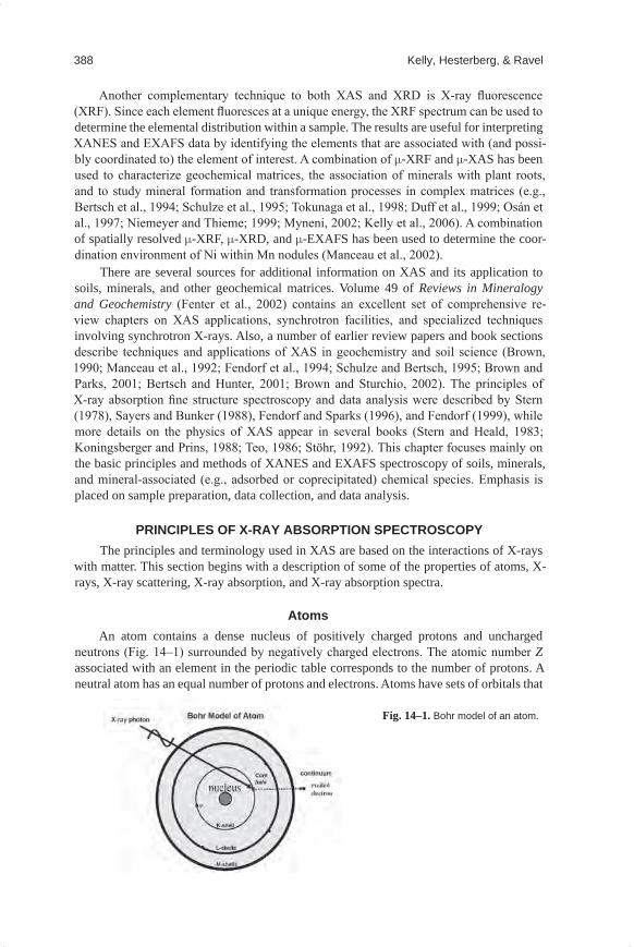
AtomsAn atom contains a dense nucleus of positively charged protons and uncharged
neutrons (Fig. 14–1) surrounded by negatively charged electrons. The atomic number Z associated with an element in the periodic table corresponds to the number of protons. A neutral atom has an equal number of protons and electrons. Atoms have sets of orbitals that
Fig.14–1.Bohr model of an atom.
Mineralogical Methods.indb 388 2/15/2008 2:37:20 PM
X-ray absorption spectroscopy 389
can be populated with electrons. The electrons occupy the orbital closest to the nucleus first because this orbital has the lowest energy. Then the other orbitals are populated in order of increasing energy. The energy required to remove an electron from an atom is the electron binding energy. The binding energy of an electron in a lower-energy orbital that is closer to the nucleus is greater than the binding energy of an electron in a higher-energy orbital that is farther from the nucleus because the inner electrons screen the positively charged nucleus from the outer electrons.
There are generally two groups of electrons associated with an atom. The loosely bound “valence” electrons occupy the outermost orbitals and participate in chemical bonding, and the tightly bound “core” electrons occupy the innermost orbitals that are an integral part of the atom. Different oxidation states of an atom are determined by charge imbalances caused by the removal of the outermost electrons. For example, Cr(0), Cr(III), and Cr(VI) have lost zero, three, and six electrons, respectively, and Cr(VI) is in a higher oxidation state than Cr(III) or Cr(0).
X-raysX-rays belong to a class of particles termed photons, which are electromagnetic ra-
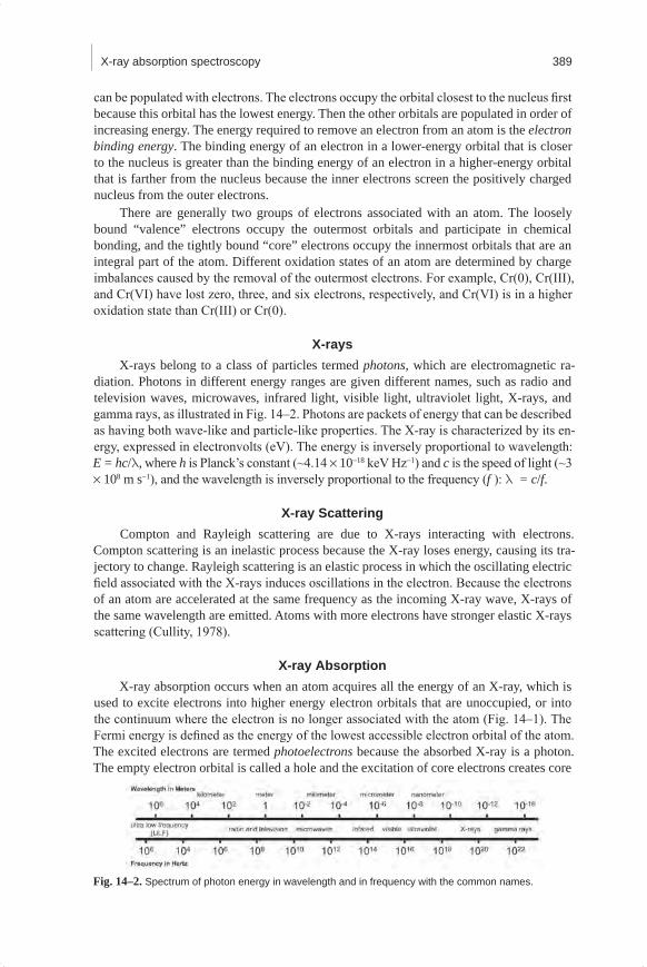
diation. Photons in different energy ranges are given different names, such as radio and television waves, microwaves, infrared light, visible light, ultraviolet light, X-rays, and gamma rays, as illustrated in Fig. 14–2. Photons are packets of energy that can be described as having both wave-like and particle-like properties. The X-ray is characterized by its en-ergy, expressed in electronvolts (eV). The energy is inversely proportional to wavelength: E = hc/l, where h is Planck’s constant (~4.14 × 10⁻¹⁸ keV Hz−1) and c is the speed of light (~3 × 10⁸ m s−1), and the wavelength is inversely proportional to the frequency (f ): l = c/f.
X-ray ScatteringCompton and Rayleigh scattering are due to X-rays interacting with electrons.
Compton scattering is an inelastic process because the X-ray loses energy, causing its tra-jectory to change. Rayleigh scattering is an elastic process in which the oscillating electric field associated with the X-rays induces oscillations in the electron. Because the electrons of an atom are accelerated at the same frequency as the incoming X-ray wave, X-rays of the same wavelength are emitted. Atoms with more electrons have stronger elastic X-rays scattering (Cullity, 1978).
X-ray AbsorptionX-ray absorption occurs when an atom acquires all the energy of an X-ray, which is
used to excite electrons into higher energy electron orbitals that are unoccupied, or into the continuum where the electron is no longer associated with the atom (Fig. 14–1). The Fermi energy is defined as the energy of the lowest accessible electron orbital of the atom. The excited electrons are termed photoelectrons because the absorbed X-ray is a photon. The empty electron orbital is called a hole and the excitation of core electrons creates core
Fig.14–2.Spectrum of photon energy in wavelength and in frequency with the common names.
Mineralogical Methods.indb 389 2/15/2008 2:37:20 PM
390 Kelly, Hesterberg, & Ravel
holes. A relaxation process occurs with the release of energy as an electron transitions from a higher-energy electron orbital to fill the core hole. In the next subsections, we discuss the properties of these electronic transitions in more detail as a prelude to subsequent sections outlining the measurement and interpretation of X-ray absorption spectra.
Electron TransitionsThe energy state of an electron is defined by quantum numbers: the principal (n = 1,
2, 3,…), the azimuthal (ℓ = 0, 1, 2, …, n − 1), and the total angular momentum (j = ℓ + s), which depends on spin (s = +1/2 or −1/2). Electrons populate these states by filling the low-est energy states first, starting with principle quantum number n = 1. The principal quantum number defines the electronic shell designated by the letters K-shell (n = 1), L-shell (n = 2), M-shell (n = 3), and so forth, as shown in Fig. 14–1. The azimuthal quantum numbers ℓ = 0, 1, 2, 3, up to n − 1 correspond to the letters s, p, d, f and are used to define the subshell of the electron. An electronic subshell is designated by n(number)l(letter)j. For example, the K shell (n = 1) has a single subshell denoted 1s (n = 1, ℓ = 0). The L shell (n = 2) can contain the 2s (n = 2, ℓ = 0), 2p1/2 (n = 2, ℓ = 1, s = −1/2, j = 1/2), and 2p3/2 (n = 2, ℓ = 1, s
= 1/2, j = 3/2) subshells corresponding to the LI, LII, and LIII subshells, respectively. The M shell (n = 3) can contain the 3s, 3p1/2, 3p3/2, and 3d3/2 and 3d5/2 subshells corresponding to the MI, MII, MIII, MIV, and MV subshells, respectively.
Electronic transitions due to X-ray absorption are restricted by the dipole selection rule such that angular momentum is conserved. This rule states that transitions can occur only between energy states that differ in the azimuthal quantum number (l) by ±1. For ex-ample, transitions from a p orbital (ℓ = 1) to an s orbital (l = 0) and vice-versa are allowed, but a transition from a 2s orbital (n = 2, ℓ = 0) to a 1s orbital (n = 1, ℓ = 0) is not allowed.
Relaxation ProcessesThe promotion of an electron into a higher energy state by X-ray absorption is short
lived. Within approximately a femto-second (10−15 s), the core hole is filled by an electron that transitions from a higher energy orbital. The transition is accompanied by a release of energy. The energy released can be in the form of fluorescence radiation, Auger electron production, or secondary electron or photon production (Teo, 1986).
X-ray fluorescence occurs when an electron from a higher-energy orbital fills the core hole by releasing an X-ray. The energy of the fluorescent X-ray is equal to the difference in the energy of the two orbitals. Because the electron orbital energies of each element are unique, the fluorescence X-ray energies for a given electronic transition will be unique for each element.
Auger electron production occurs when an electron from a higher-energy orbital fills a core hole, losing its energy by the emission of another electron from the same or a different atomic shell. Other relaxation processes include secondary electron or photon production, resulting from multiple steps of electrons cascading downward in energy as successive core holes are filled (L shell → K shell, M-shell → L-shell, etc.), with one of these multi-step processes emitting an electron or photon.
X-ray Absorption CoefficientThe number of X-rays transmitted (It) through a sample is given by the intensity of X-
rays impinging on the sample (I0) decreased exponentially by the thickness of the sample (x) and the absorption coefficient of the sample (m)
It = I0e−µx [1]
Mineralogical Methods.indb 390 2/15/2008 2:37:21 PM
X-ray absorption spectroscopy 391
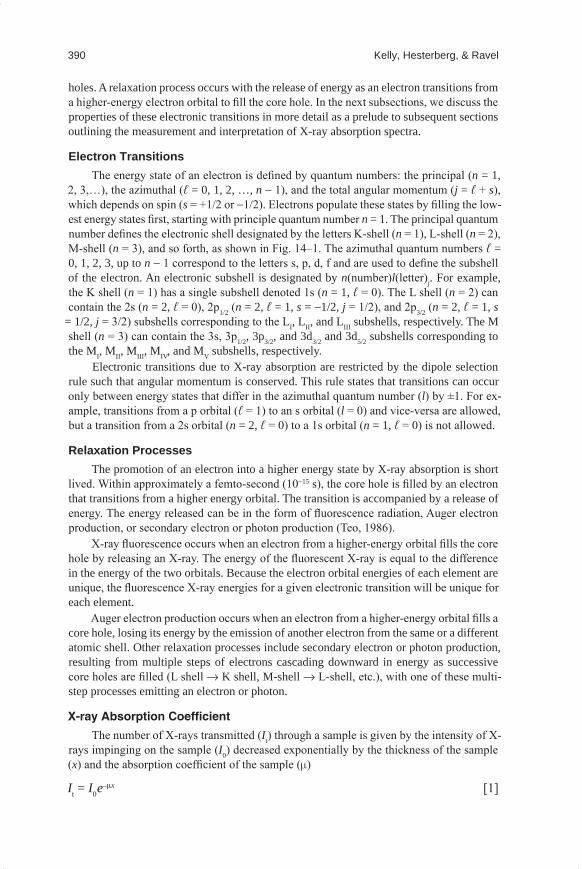
The absorption of X-rays by a material is designated by the percentage decrease in the inci-dent X-ray intensity (I0) or by the energy-dependent absorption length of the material that is the exponential factor, mx. From Eq. [1] it is apparent that as twice as many X-rays are shined on a sample, twice as many X-rays will go through the sample. This affect is linear. Also, a thicker sample will transmit fewer X-rays than a thin sample. This effect is expo-nential, such that increasing the thickness of the sample by one absorption length decreases the transmitted X-ray intensity by ~63% (100% × 1 −e−1). The absorption coefficient is a property of all elements within the sample. Elements such as Pb have greater X-ray absorp-tion coefficients than lighter elements such as O and are therefore used for efficient X-ray shielding. In radiography, an X-ray beam is impinged on the human body. The more-dense bones containing higher-Z elements like Ca absorb more X-rays than the less-dense flesh containing mainly lower-Z elements like C, H, and O. The result is a contrast image on X-ray sensitive film placed behind the subject.
The X-ray absorption coefficient (m) is the probability for an X-ray to be absorbed by a sample. X-ray absorption spectroscopy involves measuring m as a function of X-ray en-ergy. A typical experimental setup for XAS is shown in Fig. 14–3A. The X-rays go through an ionization chamber to measure the number of incident X-rays (I0), then through the sample, and then through another ionization chamber to measure the number of transmit-ted X-rays (It). The X-ray absorption coefficient is determined by rearranging Eq. [1]:
0
tln Ix =
I
æ ö÷ç ÷çm ÷ç ÷÷çè ø [2a]
Fig.14–3.(A) Picture and schematic drawing of an EXAFS experimental setup. (B) Fluorescence sample geometry and detector.
Mineralogical Methods.indb 391 2/15/2008 2:37:21 PM
392 Kelly, Hesterberg, & Ravel
Because core hole production and consequent relaxation processes are proportional to ab-sorption, the absorption coefficient can also be derived from the number of fluorescence X-rays (If):
f
0
IxI
m µ [2b]
The absorption coefficient (m) is a function of the incident X-ray energy. The prob-ability for absorption increases sharply when the incident X-ray energy equals the energy required to excite an electron to an unoccupied electron orbital. These steps in the absorp-tion coefficient are termed absorption edges.
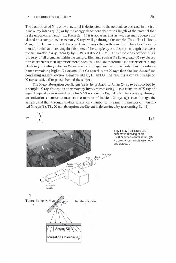
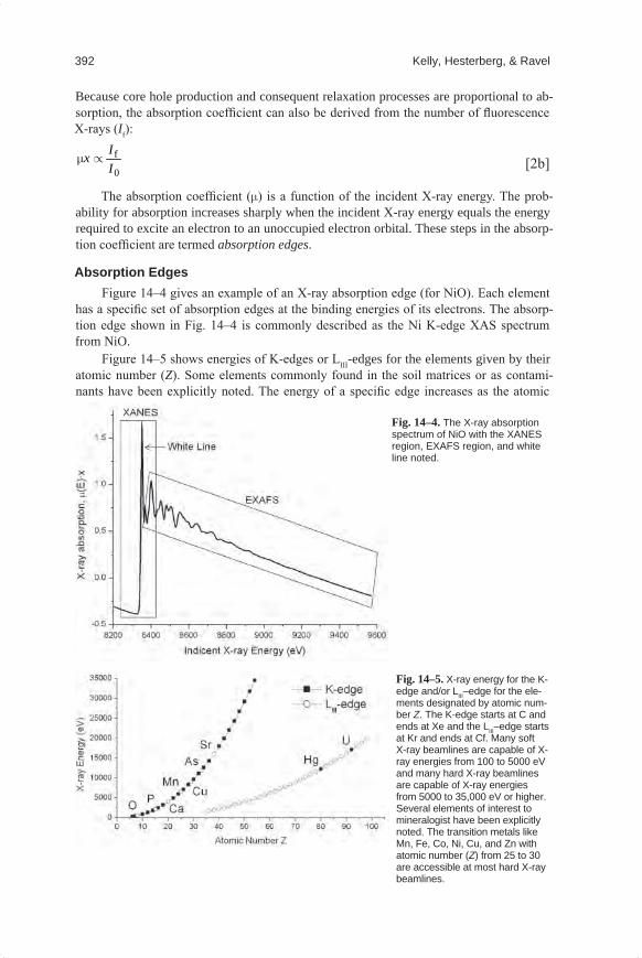
Absorption EdgesFigure 14–4 gives an example of an X-ray absorption edge (for NiO). Each element
has a specific set of absorption edges at the binding energies of its electrons. The absorp-tion edge shown in Fig. 14–4 is commonly described as the Ni K-edge XAS spectrum from NiO.
Figure 14–5 shows energies of K-edges or LIII-edges for the elements given by their atomic number (Z). Some elements commonly found in the soil matrices or as contami-nants have been explicitly noted. The energy of a specific edge increases as the atomic
Fig.14–5. X-ray energy for the K-edge and/or LIII–edge for the ele-ments designated by atomic num-ber Z. The K-edge starts at C and ends at Xe and the LIII–edge starts at Kr and ends at Cf. Many soft X-ray beamlines are capable of X-ray energies from 100 to 5000 eV and many hard X-ray beamlines are capable of X-ray energies from 5000 to 35,000 eV or higher. Several elements of interest to mineralogist have been explicitly noted. The transition metals like Mn, Fe, Co, Ni, Cu, and Zn with atomic number (Z) from 25 to 30 are accessible at most hard X-ray beamlines.
Fig.14–4.The X-ray absorption spectrum of NiO with the XANES region, EXAFS region, and white line noted.
Mineralogical Methods.indb 392 2/15/2008 2:37:23 PM
X-ray absorption spectroscopy 393
number of the element increases. This is because elements with greater atomic numbers have more positively charged nuclei from a greater number of protons, and therefore, they have a greater binding energy of an electron in a given atomic orbital. The K-shell elec-trons are closest to the atom’s nucleus (Fig. 14–1), and therefore they have greater binding energy than the L-shell electrons, as shown in Fig. 14–5 for the elements with atomic numbers 35 to 50.
Comprehensive tables of X-ray edge energies are available (e.g., McMaster et al., 1969; Shaltout et al., 2005; Elam et al., 2002). A simple graphical interface based on these tables is accessible through the program HEPHAESTUS by Ravel and Newville (2005).
X-ray Absorption SpectraA typical X-ray absorption spectrum is shown in Fig. 14–4. A full spectrum is col-
lected from approximately 200 eV below an absorption edge of interest to approximately 1000 eV above the edge.
XANES SpectraThe X-ray absorption near edge structure (XANES) is the part of the absorption spec-
trum near an absorption edge, ranging from approximately −50 to +200 eV relative to the edge energy (Fig. 14–4). The shape of the absorption edge is related to the density of states available for the excitation of the photoelectron. Therefore, the binding geometry and the oxidation state of the atom affect the XANES part of the absorption spectrum.
For most elements the absorption edge looks mostly like a step, as shown in Fig. 14–4. This absorption edge has the properties that it is linear and smooth below the absorption edge, increases sharply at the edge (like a step), and then oscillates above the edge. The main “step-like” feature of the absorption edge is due to the excitation of the photoelectron into the continuum (Fig. 14–1). The absorption edge for some elements includes decora-tions in the region of the step. These decorations may be isolated peak(s), shoulder(s), or a strong peak at the top of the step, called a “white” line. The Ni K-edge spectrum in Fig. 14–4 shows an example of a white line. Different features are caused by differences in the density of unoccupied electron orbitals that can be occupied by the excited photoelectron.
The absorption edge energy is defined as a specific energy on the step-like part of the absorption edge spectrum. The edge energy for an element in a higher oxidation state is usually shifted by up to several electronvolts to a higher X-ray energy. In a neutral atom, the positive charge of the nucleus is screened by the negative charge of the electrons. In an atom of higher oxidation state with fewer electrons than protons, the energy states of the remaining electrons are lowered slightly, which causes the absorption edge energy to in-crease. That is, an X-ray with slightly greater energy is required to excite the core electron.
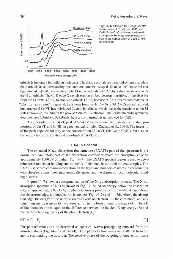
The change in element oxidation state is usually accompanied by a change in centro-symmetry, which will change the features of the absorption edge. A well-known example of a geochemical species exhibiting an isolated peak in the absorption spectrum before the step is hexavalent Cr [Cr(VI)], which exhibits a sharp peak at approximately 5994 eV (Fig. 14–6). For Cr(VI), the Fermi energy is just below the peak at 5994 eV and the continuum is the energy of the step at ~6005 eV. The peak before the edge is sometimes called a “pre-edge” peak, but we contend that this terminology is misleading because the peak is part of the absorption process, and hence it is part of the absorption edge of Cr(VI).
The origin of the Cr(VI) peak at 5994 eV can be understood in terms of its molecular orbital configuration. A neutral Cr atom in the ground state has an electronic configuration denoted as [Ar]4s23d4. The Cr atom also has 4p orbitals that are empty. Symmetry of the
Mineralogical Methods.indb 393 2/15/2008 2:37:23 PM
394 Kelly, Hesterberg, & Ravel
orbitals is important for building molecules. The d and s orbitals are threefold symmetric, while the p orbitals have directionality; the latter are dumbbell shaped. To make the tetrahedral con-figuration of Cr(VI)O3 stable, the empty 3d and 4p orbitals of Cr(VI) hybridize and overlap with the O 2p orbitals. The Cr K-edge X-ray absorption probes electron transitions of the absorber from the 1s orbital (ℓ = 0) to empty 4p orbitals (ℓ = 1) because D ℓ = ±1 as discussed above in
“Electron Transitions.” In general, transitions from the 1s (ℓ = 0) to 3d (ℓ = 2) are not allowed, but tetrahedral Cr(VI) has hybridized 3d and 4p orbitals, which makes the transition to the 3d states allowable, resulting in the peak at 5994 eV. Octahedral Cr(III) with threefold symmetry does not have hybridized 3d orbitals; hence, this transition is not allowed for Cr(III).
The intensity of the Cr(VI) peak at 5994 eV has been used to quantify the relative pro-portions of Cr(VI) and Cr(III) in geochemical samples (Zachara et al., 2004). The intensity of the peak depends not only on the concentration of Cr(VI) relative to Cr(III), but also on the symmetry of the tetrahedral coordinated Cr(VI) atom.
EXAFS SpectraThe extended X-ray absorption fine structure (EXAFS) part of the spectrum is the
normalized oscillatory part of the absorption coefficient above the absorption edge to approximately 1000 eV or higher (Fig. 14–7). The EXAFS spectral region is used to deter-mine local molecular bonding environments of elements in soils and mineral samples. The EXAFS spectrum contains information on the types and numbers of atoms in coordination with absorber atoms, their interatomic distances, and the degree of local molecular bond-ing disorder.
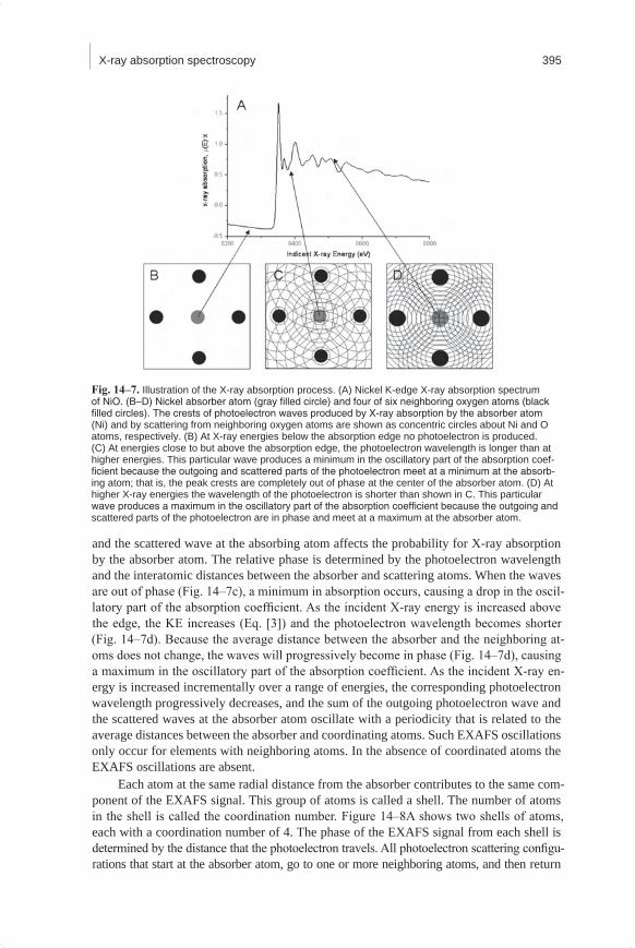
Figure 14–7 shows a conceptualization of the X-ray absorption process. The X-ray absorption spectrum of NiO is shown in Fig. 14–7a. At an energy below the absorption edge at approximately 8333 eV, no photoelectron is produced (Fig. 14–7b). At and above the absorption edge, a photoelectron is created (Fig. 14–7c and 14–7d). Above the absorp-tion edge, the energy of the X-ray is used to excite an electron into the continuum, and any remaining energy is given to the photoelectron in the form of kinetic energy (KE). The KE of the photoelectron is equal to the difference between the incident X-ray energy (E) and the electron binding energy of the photoelectron (E0):
KE = E − E0 [3]
The photoelectrons can be described as spherical waves propagating outward from the absorber atoms (Fig. 14–7c and 14–7d). These photoelectron waves are scattered from the atoms surrounding the absorber. The relative phase of the outgoing photoelectron wave
Fig.14–6. Stacked Cr K-edge spectra for mixtures of Cr(VI) from CrO3 and Cr(III) from Cr2O3 showing systematic changes in the edge region in propor-tion to the composition of each Cr oxi-dation state.
Mineralogical Methods.indb 394 2/15/2008 2:37:23 PM
X-ray absorption spectroscopy 395
and the scattered wave at the absorbing atom affects the probability for X-ray absorption by the absorber atom. The relative phase is determined by the photoelectron wavelength and the interatomic distances between the absorber and scattering atoms. When the waves are out of phase (Fig. 14–7c), a minimum in absorption occurs, causing a drop in the oscil-latory part of the absorption coefficient. As the incident X-ray energy is increased above the edge, the KE increases (Eq. [3]) and the photoelectron wavelength becomes shorter (Fig. 14–7d). Because the average distance between the absorber and the neighboring at-oms does not change, the waves will progressively become in phase (Fig. 14–7d), causing a maximum in the oscillatory part of the absorption coefficient. As the incident X-ray en-ergy is increased incrementally over a range of energies, the corresponding photoelectron wavelength progressively decreases, and the sum of the outgoing photoelectron wave and the scattered waves at the absorber atom oscillate with a periodicity that is related to the average distances between the absorber and coordinating atoms. Such EXAFS oscillations only occur for elements with neighboring atoms. In the absence of coordinated atoms the EXAFS oscillations are absent.
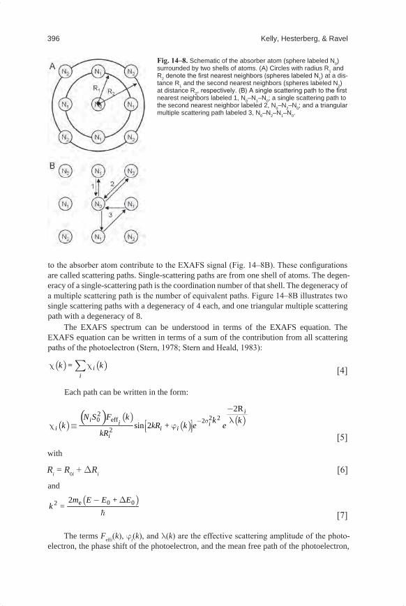
Each atom at the same radial distance from the absorber contributes to the same com-ponent of the EXAFS signal. This group of atoms is called a shell. The number of atoms in the shell is called the coordination number. Figure 14–8A shows two shells of atoms, each with a coordination number of 4. The phase of the EXAFS signal from each shell is determined by the distance that the photoelectron travels. All photoelectron scattering configu-rations that start at the absorber atom, go to one or more neighboring atoms, and then return
Fig. 14–7. Illustration of the X-ray absorption process. (A) Nickel K-edge X-ray absorption spectrum of NiO. (B–D) Nickel absorber atom (gray filled circle) and four of six neighboring oxygen atoms (black filled circles). The crests of photoelectron waves produced by X-ray absorption by the absorber atom (Ni) and by scattering from neighboring oxygen atoms are shown as concentric circles about Ni and O atoms, respectively. (B) At X-ray energies below the absorption edge no photoelectron is produced. (C) At energies close to but above the absorption edge, the photoelectron wavelength is longer than at higher energies. This particular wave produces a minimum in the oscillatory part of the absorption coef-ficient because the outgoing and scattered parts of the photoelectron meet at a minimum at the absorb-ing atom; that is, the peak crests are completely out of phase at the center of the absorber atom. (D) At higher X-ray energies the wavelength of the photoelectron is shorter than shown in C. This particular wave produces a maximum in the oscillatory part of the absorption coefficient because the outgoing and scattered parts of the photoelectron are in phase and meet at a maximum at the absorber atom.
Mineralogical Methods.indb 395 2/15/2008 2:37:24 PM
396 Kelly, Hesterberg, & Ravel
to the absorber atom contribute to the EXAFS signal (Fig. 14–8B). These configurations are called scattering paths. Single-scattering paths are from one shell of atoms. The degen-eracy of a single-scattering path is the coordination number of that shell. The degeneracy of a multiple scattering path is the number of equivalent paths. Figure 14–8B illustrates two single scattering paths with a degeneracy of 4 each, and one triangular multiple scattering path with a degeneracy of 8.
The EXAFS spectrum can be understood in terms of the EXAFS equation. The EXAFS equation can be written in terms of a sum of the contribution from all scattering paths of the photoelectron (Stern, 1978; Stern and Heald, 1983):
( ) ( )ii
k = kc cå [4]
Each path can be written in the form:
( )( ) ( )
( ) ( )2 2 20 eff 2
2
2R
sin 2
ii i i
i i ii
N S F k k kk kR + k e ekR
- s
-lé ùc º jê úë û
[5]
with
Ri = R0i + DRi [6]
and
( )e 0 02 2m E E + Ek =
- D
[7]
The terms Feffi(k), ji(k), and l(k) are the effective scattering amplitude of the photo-electron, the phase shift of the photoelectron, and the mean free path of the photoelectron,
Fig. 14–8. Schematic of the absorber atom (sphere labeled N0) surrounded by two shells of atoms. (A) Circles with radius R1 and R2 denote the first nearest neighbors (spheres labeled N1) at a dis-tance R1 and the second nearest neighbors (spheres labeled N2) at distance R2, respectively. (B) A single scattering path to the first nearest neighbors labeled 1, N0–N1–N0; a single scattering path to the second nearest neighbor labeled 2, N0–N2–N0; and a triangular multiple scattering path labeled 3, N0–N2–N1–N0.
Mineralogical Methods.indb 396 2/15/2008 2:37:24 PM
X-ray absorption spectroscopy 397
respectively, all of which can be calculated by a computer program such as FEFF (Rehr and Albers 2000). The term Ri is the half path length of the photoelectron (i.e., the distance be-tween the absorber and a coordinating atom for a single-scattering event). The value of R0i is the half path length used in the theoretical calculation which can be modified by DRi. The re-maining variables, described below, are usually determined by modeling the EXAFS spectrum. Equation [7] is used to express the excess KE of the photoelectron in wavenumber, k, by using the mass of the electron me and Plank’s constant . It is helpful to note that
(E − E0) ≈ 3.81k2 [8]
where (E − E0) is in units of electronvolts, and k is in units of Å−1.The EXAFS equation is easiest to understand for a single scattering path. Each of its
terms is described below.
(NiS02): These terms modify the amplitude of the EXAFS signal and do not
have a k-dependence. The subscript i indicates that this value can be different for each path of the photoelectron. For single scattering, Ni represents the number of coordinating atoms within a particular shell. For multiple scattering, Ni represents the number of identical paths. The passive electron reduction factor (S0
2) usually has a value between 0.7 and 1.0 (Li et al., 1995). S0
2 accounts for the slight relaxation of the remaining electrons in the presence of the core hole vacated by the photoelectron. S0
2 is different for different elements, but the value is generally transferable between different species from the same element and the same edge.
Feffi(k): This term is the effective scattering amplitude. For a single scattering path
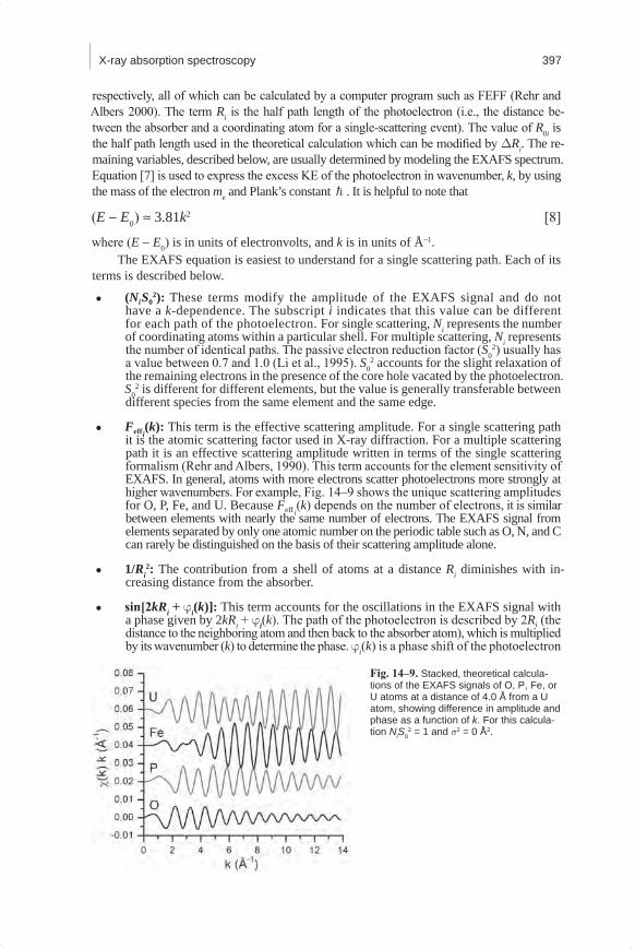
it is the atomic scattering factor used in X-ray diffraction. For a multiple scattering path it is an effective scattering amplitude written in terms of the single scattering formalism (Rehr and Albers, 1990). This term accounts for the element sensitivity of EXAFS. In general, atoms with more electrons scatter photoelectrons more strongly at higher wavenumbers. For example, Fig. 14–9 shows the unique scattering amplitudes for O, P, Fe, and U. Because Feff i
(k) depends on the number of electrons, it is similar between elements with nearly the same number of electrons. The EXAFS signal from elements separated by only one atomic number on the periodic table such as O, N, and C can rarely be distinguished on the basis of their scattering amplitude alone.
1/Ri2: The contribution from a shell of atoms at a distance Ri diminishes with in-
creasing distance from the absorber.
sin[2kRi + ji(k)]: This term accounts for the oscillations in the EXAFS signal with a phase given by 2kRi + ji(k). The path of the photoelectron is described by 2Ri (the distance to the neighboring atom and then back to the absorber atom), which is multiplied by its wavenumber (k) to determine the phase. ji(k) is a phase shift of the photoelectron
·
·
·
·
Fig. 14–9. Stacked, theoretical calcula-tions of the EXAFS signals of O, P, Fe, or U atoms at a distance of 4.0 Å from a U atom, showing difference in amplitude and phase as a function of k. For this calcula-tion NiS0
2 = 1 and s2 = 0 Å2.
Mineralogical Methods.indb 397 2/15/2008 2:37:25 PM
398 Kelly, Hesterberg, & Ravel
caused by the interaction of the photoelectron with the nuclei of the absorber atom and the interaction with the nuclei of the coordinating atoms of the photoelectron path. Because the photoelectron has a negative charge and the nucleus is positively charged, the photoelectron loses energy and its wavelength lengthens as it interacts with the coordinating atoms and the absorber atom. It is this sine term in the EXAFS equation that makes the Fourier transform (FT) of the XAFS signal such a powerful tool, because a FT results in peaks at distances related to Ri, the interatomic dis-tances between the absorber and coordinating atoms. The peak is not precisely at Ri due to the phase shift j(k), which causes a shift in distance of approximately −0.5 Å.
e−2σi2k2: Because all of the coordinating atoms in a shell are not fixed at positions of
exactly a distance Ri from the central absorber atom, s2 accounts for the disorder in the interatomic distances. s2 is the mean-square displacement of the bond length between the absorber atom and the coordination atoms in a shell. This term has contributions from dynamic (thermal) disorder as well as static disorder (structural heterogeneity). A distribution of distances within a single shell decreases the am-plitude of the EXAFS signal because the phase differences between outgoing and scattered photoelectrons are shifted slightly for each atom in the coordination shell. The EXAFS process occurs on the femto-second (10-15 s) time scale, while thermal vibrations occur on a much longer time scale of 10−10 to 10−12 s. Because the atoms are essentially “frozen” at one position about their thermodynamic minima during the excitation process, EXAFS spectra measure the distribution of the distances be-tween the absorber atom and each of the coordinating atoms within a shell in terms of a s2 value. The static disorder component of s2 is due to differences in the posi-tion of the minima themselves. Thus, for example, if two interatomic distances are separated by only 0.010 Å, with one atom at 2.00 Å and another atom at 2.10 Å, the contributing EXAFS signal could be modeled with one scattering path at 2.05 Å with a mean disorder of 0.05 Å such that there is an additional s2 term due to the static disorder of 0.0025 Å2.
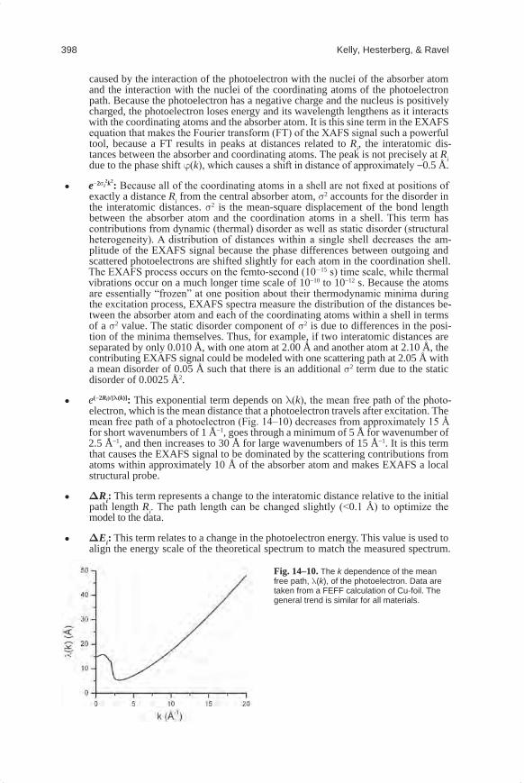
e(−2Ri)/[l(k)]: This exponential term depends on l(k), the mean free path of the photo-electron, which is the mean distance that a photoelectron travels after excitation. The mean free path of a photoelectron (Fig. 14–10) decreases from approximately 15 Å for short wavenumbers of 1 Å−1, goes through a minimum of 5 Å for wavenumber of 2.5 Å−1, and then increases to 30 Å for large wavenumbers of 15 Å−1. It is this term that causes the EXAFS signal to be dominated by the scattering contributions from atoms within approximately 10 Å of the absorber atom and makes EXAFS a local structural probe.
DRi: This term represents a change to the interatomic distance relative to the initial path length Ri. The path length can be changed slightly (<0.1 Å) to optimize the model to the data.
DEi: This term relates to a change in the photoelectron energy. This value is used to align the energy scale of the theoretical spectrum to match the measured spectrum.
·
·
·
·
Fig.14–10.The k dependence of the mean free path, l(k), of the photoelectron. Data are taken from a FEFF calculation of Cu-foil. The general trend is similar for all materials.
Mineralogical Methods.indb 398 2/15/2008 2:37:25 PM
X-ray absorption spectroscopy 399
The value of DEi can differ between coordination shells, but is more often a constant for all paths used in the model.
X-RAY ABSORPTION MEASUREMENTSThis section is aimed at facilitating the design and implementation of successful X-
ray absorption measurements. There are many general practices given in the first section “Design of an X-ray Absorption Project.” Typical components of a synchrotron and X-ray beamline are described in “Synchrotron Facilities” and “X-ray Beamlines,” respectively. The final section describes several detailed methods for sample preparation and sample measurements. There are many requirements for a successful X-ray absorption project; therefore, it is often desirable to collaborate with an expert that can be found through the synchrotron facility or at www.xafs.org (verified 17 Dec. 2007).
Design of an X-ray Absorption ProjectX-ray absorption is potentially useful for a broad array of specialized problems in soil
mineralogy and soil chemistry with varying objectives. The need for an X-ray absorption experiment usually begins with the hypothesis that there is an element(s) with a particular local atomic configuration and/or valence state that is affecting the macroscopic behavior of the system. Key factors to consider in the design of a project are the identification of absorber atom(s), their concentration, the absorption edge and data collection method, and the data analysis method. In general, there are two different methods of X-ray absorption analysis. The first method is based on comparing unknown spectra with those of well-char-acterized, physical “standards.” The second method involves comparing or modeling the spectrum for an unknown sample with theoretically calculated spectra. Usually a combi-nation of these two techniques is used for EXAFS analysis, while XANES analysis relies heavily on comparisons with standards. For EXAFS analysis, spectra for physical stan-dards can be used to make comparisons, optimize the theoretical models, and assess the performance of the beamline.
Often projects involve multiple elements that are affected by some physical, chemical, or biological process. Analyzing two or more elements is particularly useful if it is sus-pected that these elements are coordinated to each other. Consider, for example, a project that involves understanding coprecipitation of Zn with Fe oxides in a contaminated soil or subsurface undergoing redox fluctuations. If 15 mol% or more of the Fe(III) within a poorly crystalline Fe oxide is substituted by Zn(II), then Fe K-edge and Zn K-edge EXAFS measurements on the same sample would potentially produce a well-constrained data set. The Zn EXAFS spectra will contain a signal from the Fe neighbors, and the Fe EXAFS spectra will contain a corresponding signal from the Zn neighbors.
The concentration of the absorber atom may limit data collection to the XANES part of the absorption spectrum. The XANES spectrum contains the signal of the absorption edge itself, while the EXAFS represents only about 10% or less of that (Fig. 14–4). As discussed in a later section, approximately 100 to 1000 times more atoms of the absorber element are required for EXAFS than for XANES. Hence, the number of absorber atoms per unit volume is needed to determine the feasibility of an X-ray absorption experiment. In the example given above, if the concentration of Zn substituted into Fe oxide is <0.01 mol%, then the Zn K-edge measurement becomes difficult, as it requires long measurement times to obtain the required measurement statistics. In addition, if the concentration of Zn is <10 mol%, then the Fe K-edge EXAFS sig-nal will contain very little signal from the Zn atoms because an insufficient number of the Fe
Mineralogical Methods.indb 399 2/15/2008 2:37:25 PM
400 Kelly, Hesterberg, & Ravel
neighboring atoms will be Zn. Even so, the Fe K-edge EXAFS signal may still be useful in quantifying the affect of Zn on the Fe oxide.
X-ray absorption spectra can be collected at more than one edge of one particular element. Many hard X-ray energy edges are well separated by 1000 eV or more, which is essential for EXAFS spectroscopy. Edges at low X-ray energies are typically separated by several hundred electronvolts or less. These edges are suitable for XANES analysis. If an element’s oxidation state is of primary interest, then the spectrum at a lower-energy edge might show a larger shift in the edge position with changing oxidation state or centrosym-metry than the spectra at a higher-energy edge. The elements O, N, and C have low-energy XANES spectra with characteristic features that can be used to differentiate the number and types of bonding environments.
Standards chosen for an XAS project usually include well-characterized minerals, ad-sorbed phases, or aqueous species that contain the element of interest in chemical forms that are considered relevant to the system studied with respect to mineralogy, chemical composition, and pH. The ideal XAS standards exactly match all aspects of the chemical species in the sample. However, it is not possible to synthesize or purchase standards, such as minerals or noncrystalline solids, that match the crystallinity, impurities, and defect structures of similar phases that were formed or degraded under the unique weathering conditions of a soil. In fact, it is often the project objective to determine these aspects of soil minerals. Therefore, a reasonable set of chemically meaningful standards should be included. Through the modeling of standards, the EXAFS signal can be understood and used to help constrain the structural model for the unknown sample. In the example of Zn substituted into an Fe oxide, a set of standards might include various synthesized Fe oxide minerals with different concentrations of coprecipitated Zn, and one or more Zn oxide or Zn hydroxide and Zn-free Fe oxide minerals. In addition, a metallic Zn-foil and Fe-foil are usually included to assess the quality of the beamline settings.
Synchrotron Radiation FacilitiesX-ray absorption spectroscopy measurements are made at synchrotron radiation facil-
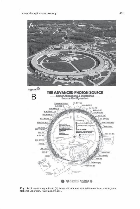
ities. As of 2002, there were approximately 50 synchrotron radiation facilities in operation or under construction around the world (Sham and Rivers, 2002). Synchrotron X-ray fa-cilities are grouped in terms of generations (currently first, second, and third generation) based on the technologies that result in a general range of capabilities. In the United States, there are four second- or third-generation synchrotron user DOE-funded facilities, includ-ing the Advanced Photon Source (APS) at Argonne National Laboratory (Fig. 14–11), the National Synchrotron Light Source (NSLS) at Brookhaven National Laboratory, the Stanford Synchrotron Radiation Laboratory (SSRL) at Stanford Linear Accelerator Center, and the Advanced Light Source (ALS) at Berkeley Laboratory. A third-generation facility at Brookhaven National Laboratory is being planned. Additional information, including details on gaining access to these facilities through peer review of proposals, is available online at www.lightsources.org (verified 17 Dec. 2007).
A schematic overview of a synchrotron facility is depicted in Fig. 14–11B. Bunches of charged particles are initially accelerated by a linear accelerator (LINAC) and then acceler-ated further in a booster ring that injects the particles traveling near the speed of light into a storage ring (Fig. 14–11B). The particles within the storage ring are accelerated toward the center of the ring each time their trajectory is changed so that they travel in a closed loop. This causes X-rays with a broad spectrum of energies (white light) to be emitted tangential to the storage ring. Therefore, a synchrotron storage ring is an N-sided polygon, where N
Mineralogical Methods.indb 400 2/15/2008 2:37:25 PM
X-ray absorption spectroscopy 401
Fig.14–11. (A) Photograph and (B) Schematic of the Advanced Photon Source at Argonne National Laboratory (www.aps.anl.gov).
Mineralogical Methods.indb 401 2/15/2008 2:37:26 PM
402 Kelly, Hesterberg, & Ravel
is the number of bends. The particle trajectory is bent by magnets. Wigglers and undula-tors are two types of specialized insertion devices that are placed in the straight sections of the storage ring. These devices are an integral part of third-generation facilities. A wiggler consists of several closely spaced bending magnets that increase the intensity of the X-ray pulse. An undulator oscillates the charged particles using carefully spaced magnets such that the interference between their poles affects the emitted X-ray spectrum. This interference is additive at particular wavelengths, producing an intense X-ray beam at a wavelength that can be selected by varying the gap between the poles of the magnets. Beamlines are placed tangential to the storage ring to use the X-rays emitted by bending the charged particles. Bending-magnet and wiggler beamlines are well suited for XAS measurements because the X-ray energies produced span 1000 eV or more as needed for an XAS spectrum. To preserve the high brilliance of an undulator beamline, the spacing between the magnets is changed as the EXAFS scan is collected. With some loss of intensity, the undulator spacing can be ta-pered to produce a wider range of the X-ray energies for XAS measurements.
Beamline SetupSetting up a synchrotron beamline for XAS data collection is typically done by or
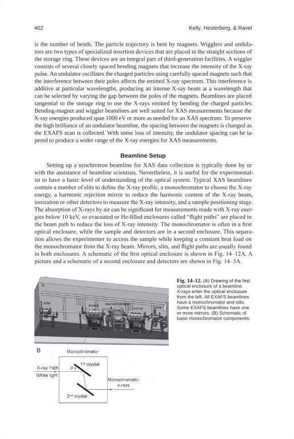
with the assistance of beamline scientists. Nevertheless, it is useful for the experimental-ist to have a basic level of understanding of the optical system. Typical XAS beamlines contain a number of slits to define the X-ray profile, a monochromator to choose the X-ray energy, a harmonic rejection mirror to reduce the harmonic content of the X-ray beam, ionization or other detectors to measure the X-ray intensity, and a sample positioning stage. The absorption of X-rays by air can be significant for measurements made with X-ray ener-gies below 10 keV, so evacuated or He-filled enclosures called “flight paths” are placed in the beam path to reduce the loss of X-ray intensity. The monochromator is often in a first optical enclosure, while the sample and detectors are in a second enclosure. This separa-tion allows the experimenter to access the sample while keeping a constant heat load on the monochromator from the X-ray beam. Mirrors, slits, and flight paths are usually found in both enclosures. A schematic of the first optical enclosure is shown in Fig. 14–12A. A picture and a schematic of a second enclosure and detectors are shown in Fig. 14–3A.
Fig.14–12. (A) Drawing of the first optical enclosure of a beamline. X-rays enter the optical enclosure from the left. All EXAFS beamlines have a monochromator and slits. Some EXAFS beamlines have one or more mirrors. (B) Schematic of basic monochromator components.
Mineralogical Methods.indb 402 2/15/2008 2:37:27 PM
X-ray absorption spectroscopy 403
The purpose of optimizing the beamline optical system is primarily to maximize the intensity of monochromatic X-rays of appropriate resolution on the sample. Also, during the XAS scan, the X-ray intensity should change smoothly and the position of the beam on the sample should remain stable. Beamline optics can move out of optimal alignment dur-ing the course of an experiment. Monitoring the incident X-ray intensity (I0) with respect to ring current can help identify misalignment problems.
SlitsSlits are used to define the X-ray beam profile and to block unwanted X-rays. Two
common types are fixed and adjustable slits. Fixed slits have a pre-cut opening of fixed heights between 0.2 and 1.0 mm and a width of several centimeters. These slits can be moved into or out of the X-ray beam. Adjustable slits use metal plates that move indepen-dently to define each edge of the X-ray beam. Many beamlines have slits located upstream and downstream of the monochromator (Fig. 14–12A) and before the I0 detector (Fig. 14–3A).
The monochromator slits may need to be adjusted at the start of an experiment or after a large (several kiloelectronvolts) change in X-ray energy. Optimization is done by maxi-mizing the X-ray intensity while changing the position of the slit opening. Vertical slits placed downstream or upstream of the monochromator can be used to increase the energy resolution of the X-ray incident on the sample at the expense of some loss in X-ray intensity.
MonochromatorThe monochromator is used to select the X-ray energy incident on the sample.
Typically the monochromator is stepped through the XAS scan range or it can be run con-tinuously. The latter scanning mode is called quick-scanning of the monochromator.
An X-ray monochromator usually consists of two parallel crystals (double-crystal monochromator) or a single crystal with a slot cut nearly through it (channel-cut mono-chromator). Typical monochromator crystals are made of silicon or germanium and are cut and polished such that a particular atomic plane of the crystal, described by the (hkl) indi-ces, is parallel to the surface of the crystal. Common monochromator crystals are Si(111), Si(311), and Ge(111). The energy of X-rays diffracted by the crystal is controlled by rotat-ing the crystals in the white beam. A simplified schematic of a monochromator is shown in Fig. 14–12B. Only the X-rays with energies that satisfy Bragg’s Law are diffracted by the crystal. Bragg’s Law is:
nl = 2d sin(q) [9]
where d is the spacing of the atomic planes of the crystal parallel to its surface, q is the angle of the crystal with respect to the impinging white beam, l is the wavelength of the diffracted X-ray, and n is an integer. The fundamental X-ray energy corresponds to n = 1, and X-rays of higher harmonic energies correspond to n > 1.
Harmonic Rejection.The harmonic X-ray intensity needs to be reduced, as these X-rays will adversely affect
the XAS measurement. Harmonic X-rays that are diffracted from the crystal depend on the crystal lattice and the cut of the crystal. It is useful to use a crystal that does not diffract the sec-ond harmonic (n = 2) because the intensity of the second harmonic is usually much greater than the intensity of the higher harmonics. Silicon crystals with the diamond structure will not allow the harmonics that satisfy the equation h + k + l = n, where n is twice an odd number. Hence, the Si(111) crystals do not diffract the second (for an odd number of 1) or sixth (for an odd num-ber of 3) harmonic. For example, by using a Si(111) crystal at 8 keV, the first allowed harmonic
Mineralogical Methods.indb 403 2/15/2008 2:37:27 PM
404 Kelly, Hesterberg, & Ravel
is at 24 keV (n = 3), rather than at 16 keV (n = 2). When working at high X-ray energies, it is possible that the energy of higher-order harmonics exceeds the maximum energy produced by the synchrotron storage ring. In that case, no harmonic rejection is needed.
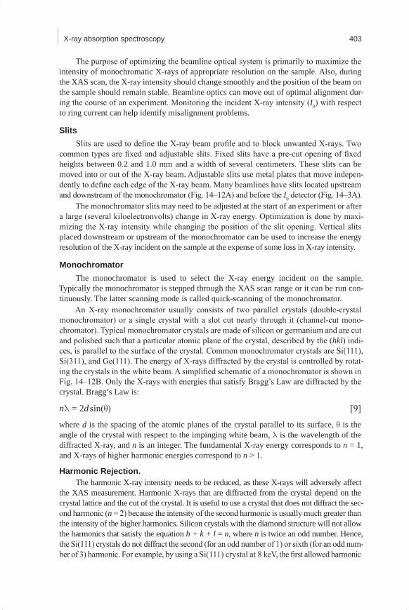
Common methods for reducing the harmonic X-ray content include detuning the sec-ond crystal of the monochromator or using a harmonic rejection mirror. To detune the monochromator, the angle of the second crystal is slightly offset with respect to the angle of the first crystal, causing the X-ray intensity to be decreased slightly for the fundamental energy while dramatically decreasing the higher harmonic intensity. Figure 14–13 shows the reflectivity of a Si(111) double crystal monochromator with and without detuning, based on calculations from Heald (1988b).
The degree of detuning is determined by the change in the incident X-ray intensity (I0) relative to its maximum value obtained for parallel crystals. For example, 20% detuning means that I0 has been decreased by 20% of its maximum value. Detuning is usually done at approximately 200 eV above the absorption edge. The beamline scientist should know the appropriate amount of detuning needed for a particular measurement. The method used at the APS to determine the harmonic content of the X-ray beam can be found at www.xafs.org. At some beamlines, the degree of detuning is not stable and needs to be monitored and regularly adjusted.
The harmonic content can be determined by monitoring the transmission intensity of a foil of one absorption length with an absorption edge just above the energy of the first al-lowed harmonic. This foil will completely block the fundamental X-rays and transmit 66% of the harmonic X-rays. The detuning angle on the second monochromator crystal can be increased until the transmitted X-ray intensity (It) is reduced appropriately.
Another common method for removing harmonic X-rays is to use a harmonic rejec-tion mirror. This mirror is usually made of Si for low energies, Rh for X-ray energies below the Rh absorption edge at 23 keV, or Pt for higher X-ray energies. The mirror is placed at a grazing angle in the beam such that the X-rays with fundamental energy are reflected toward the sample, while the harmonic X-rays are not. This is because the critical angle for reflectance depends on energy. Slits placed downstream of the mirror are used to block the direct beam containing the harmonic X-rays. The mirror angle is optimized by measur-ing the reflected beam intensity as a function of mirror angle. This measurement is usually performed at several different energies, one in the scan region and another a few kiloelec-tronvolts higher. The optimum angle of the mirror allows maximum reflection in the X-ray energy region of interest while reflecting insignificant X-rays of higher harmonics.
Fig.14–13. Reflectivity of fundamental energy of 10 KeV and the third harmonic of 30 KeV from a Si(111) monochro-mator crystal as a change in relative energy from the Bragg energy (EB) (A) without detun-ing and (B) with a detuning angle of 3.5 arcsec. The inten-sity of the third harmonic in B has been multiplied by 100.
Mineralogical Methods.indb 404 2/15/2008 2:37:27 PM
X-ray absorption spectroscopy 405
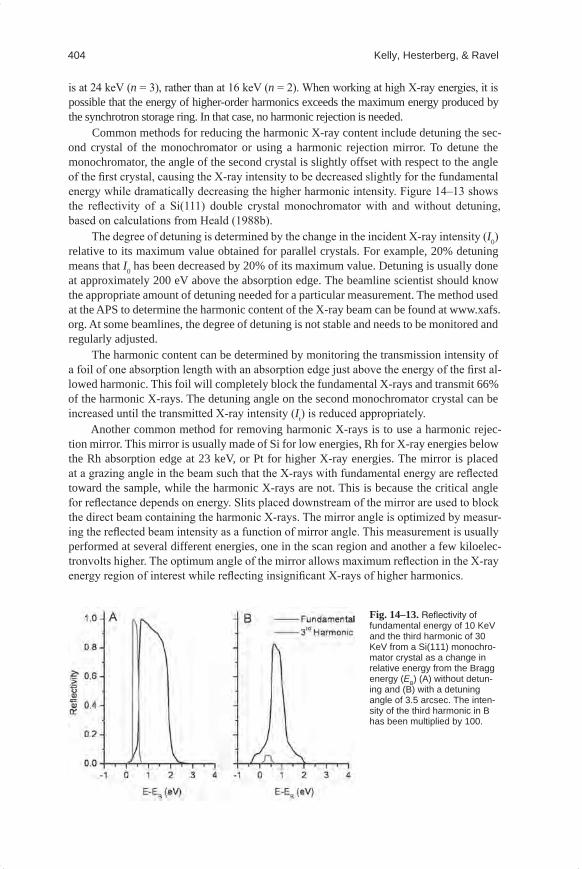
For example, Fig. 14–14 shows the relative intensities of X-rays at three different energies that are reflected from a Rh mirror as a function of mirror angle. Shallow mirror angles corresponding to mirror steps <175 reflect the X-rays at all three energies shown. X-rays with energy of 17,000 eV are reflected strongly until the mirror reaches a critical angle corresponding to mirror steps of approximately 230, then reflectivity drops sharply. Critical angles for X-rays of 18,000 and 21,000 eV correspond to approximately 220 and 180 steps, respectively, showing that the critical angle decreases with increasing energy. To reject higher harmonics during an EXAFS scan from 17,000 to 18,000 eV, the mirror angle is set to approximately 220 steps so that the mirror reflects the 17,000- and 18,000-eV x-rays, but not higher-energy X-rays.
Monochromator Calibration.The X-ray energy is determined by the angle of the monochromator crystal (Fig.
14–12B) relative to the incident X-ray beam through Bragg’s Law (Eq. [9]). Motors that control the monochomator angle can slip, causing the X-ray energy to be miscalibrated. Also, the temperature of the monochromator affects the mean crystal spacing. Therefore, the monochromator energy is typically calibrated at the start of data collection and moni-tored throughout an experiment. Usually, the energy of the X-rays is determined from the absorption edge of a reference standard. Alternatively, a sample composed of a higher-Z element with an edge falling within the energy scan is suitable for elements that are not easily obtained. For example, a Y foil (K-edge = 17,038 eV) can be used when collecting data for U (LIII–edge = 17,166 eV) with a scan region from 16,938 to 18,000 eV.
It is good practice to simultaneously monitor the monochomator X-ray energy for each XAS scan by collecting the absorption spectrum from a reference standard. The reference stan-dard is usually collected in transmission mode by using the X-rays that pass through the sample as shown in Fig. 14–3A, or by using scattered X-rays (Cross and Frenkel, 1998). By aligning the reference spectra collected with each sample spectrum, relative changes in the absorption edge energy from different chemical species can be determined accurately. For comparison of edge energy shifts of XANES spectra, there is a convention used to define an absolute energy scale relative to some feature of the absorption edge. This convention is necessary for comparing spec-tra from different studies and is discussed in the “Data Analysis” section below.
Detectors
Ionization Detectors. Typical X-ray absorption measurements use ionization detectors. Ionization detectors are gas-filled devices of typical lengths between 2 and 60 cm. Figure 14–3A shows an example of incident (I0), transmission (It), and fluorescence (If) ionization
Fig.14–14.Reflection from a Rh harmonic re-jection mirror at three different X-ray energies. The cut-off angle for a U scan from 17,000 to 18,000 eV is indicated by the arrow.
Mineralogical Methods.indb 405 2/15/2008 2:37:28 PM
406 Kelly, Hesterberg, & Ravel
chambers. Alignment is done by using a fixed-position laser or by using X-ray fluorescence material or light-sensitive (“burn”) paper placed across a detector window. After the other beamline optics are positioned, it is good practice to recheck the alignment of the detectors.
The ionization detectors contain two parallel plates separated by a gas-filled space that the X-rays travel through. Some of the X-rays ionize the gas particles. A voltage bias applied to the parallel plates separates the gas ions, creating a current. The applied voltage should give a linear detector response for a given change in the incident X-ray intensity. Linearity tests can be used to determine the response of the detectors (Kemner et al., 1994).
The ionization detectors are filled with one or two inert gases to optimize X-ray ab-sorption for a given edge energy. Absorption increases with increasing atomic number of the gas (He < N2 < Ar < Kr) and increasing detector length. In general, suitable attenuation of the X-ray intensity by the detectors is 10 to 20% for the I0 detector and 70 to 90% for the It and Iref detectors.
The gas mixture needed to achieve a given absorption is similar to that described be-low in the “Sample Preparation” section. The open source software program Hephaestus contains a calculator for determining the optimum gas mixture. Typically the ionization detector is purged with the appropriate gas mixture, and then while measurements are made the gas is slowly flowed (50–100 mL min−1) through the detector, or the gas mixture is sealed within an air tight detector.
The voltage reading (V) from the ionization chamber is proportional to the number of X-ray photons per second (NX-ray/s) passing through the detector as given by
X-ray X-ray
ion
N EV eA
s E= [10]
where e is the charge of an electron, A is the ionization detector amplifier gain, and EX-ray is the X-ray energy in electronvolts. Typical gases have an ionization energy Eion of 30 eV, so the number of X-rays per second becomes
20X-ray
X-ray
2 10N Vs AE
´= [11]
The Hephaestus software program contains a utility for calculating the number of X-rays per second.
Fluorescence Detectors. Fluorescence X-rays are usually measured at a 90° angle relative to the incident beam direction, with the sample being positioned in between at a 45° angle (Fig. 14–3B). The 90° angle between the detector and the incident beam direction is used because the fluorescence X-rays are emitted from the sample isotropically, while the intensity of the scattered X-rays is a minimum at 90° (Compton, 1923). Therefore, the greatest signal/background ratio is obtained for a 90° angle between the incident beam and the detector. Both Stern–Heald (Stern and Heald, 1979) and solid-state detectors are com-monly used in XAS analysis of soil samples. The Stern–Heald detector consists of an X-ray filter, solar slits, and a large-window ionization detector (Fig. 14–3B). The X-ray filter is used to preferentially absorb scattered X-rays from the sample and is described in more de-tail below. The solar slits consist of a fan of thin pieces of metal, the point of the fan going in the X-ray beam direction and the fingers of the fan directed from the sample position to the detector. The solar slits block X-rays that do not originate at the sample. Proper align-
Mineralogical Methods.indb 406 2/15/2008 2:37:28 PM
X-ray absorption spectroscopy 407
ment of the solar slits is critical. A commercially available Stern–Heald type of detector is shown in Fig. 14–3A. It comprises a sample chamber, solar slits, and ionization detector that are connected for automatic alignment of the solar slits.
The fluorescence filter (Heald, 1988a) for the transition metals usually consists of the element of one atomic number lower than the absorber element, and is called a “Z − 1 filter.” This is because the absorption edge of the filter has an energy between energies of the incident X-rays and the fluorescence X-rays. For example, XAS measurements of Fe may use a Mn filter of one absorption length (3 mm). The incident X-ray energy of 7200 eV is above the absorption edge of Mn at 6539 eV, such that 55% of the scattered 7200 eV X-rays are absorbed, but the fluorescent X-ray energy from the Fe at 6400 eV is below the Mn ab-sorption edge, such that only 13% of these X-rays are absorbed. Therefore, a greater ratio of fluorescent X-rays relative to the scattered X-rays reach the detector, and the measurement is improved. For elements with atomic number greater than 37 a “Z − 2” filter can be used.
A Stern–Heald detector is useful for samples with low to moderate absorber concen-trations in a matrix that has low background signal because the fluorescence ionization chamber does not discriminate X-rays on the basis of their energy. For example, a Cu (K-edge = 8979 eV) measurement as a minor element in an Fe-rich matrix (Fe K-edge = 7112 eV) will have a large background signal from the Fe. In these situations a solid-state detec-tor that can select the fluorescence X-rays from the Cu atoms is usually a better choice.
Solid-state detectors use a semiconducting material as a sensor for fluorescence X-rays. The most common solid-state XAS detector is a germanium detector, although silicon drift detectors are becoming increasingly popular. The solid-state sensor on a germanium detector is usually protected from the external environment by a thin beryllium window and is operated at liquid nitrogen temperature. Multi-element detectors (MED) have mul-tiple detectors within the sensing unit, and the fluorescence signal from each detector is collected during each scan. Because the area of the X-ray transparent window from each element subtends a different solid angle relative to the position of the incident beam on the sample, the fluorescence signal varies between elements. These differences can be used to properly align the MED to the sample.
The electronics associated with the solid-state detector allow for the X-ray energy to be determined and only those X-rays within a specified energy range to be recorded. For the example of trace amounts of Cu in an Fe matrix, the fluorescence peak from Cu at 8046 eV can be distinguished to a large degree from the fluorescence peak from Fe at 6405 eV. The biggest drawback to the MED detector is that the electronics can be overloaded by too much signal, creating “dead time” when the detector is spending time processing signal rather than collecting signal. It is best to keep the count rate as high as possible and the dead time as low as possible. A maximum dead time of 10% is usually acceptable. The signal can be internally corrected for dead time, so depending on the configuration of the particular solid-state detector, different maximum dead times may be acceptable. Common approaches to limit the dead time of an MED are to reduce the incident X-ray intensity, add low-Z filters (Teflon or Al) to preferentially absorb fluorescence from lower Z elements, or increase the distance between the sample and detector. The “Z − 1” filter is not recom-mended for the MED detector because fluorescence from the absorber element creates additional X-rays for the MED to process, and the signal from the filter can overlap with the signal from the absorber atom.
Electron Yield Detectors. An electron yield detector is particularly useful for collecting data on concentrated standards in the soft X-ray region, where Auger electron production is greater than fluorescence. Electron-yield detection is surface sensitive, and it does not
Mineralogical Methods.indb 407 2/15/2008 2:37:28 PM
408 Kelly, Hesterberg, & Ravel
suffer from self-absorption effects, described in the section “Fluorescence Mode Samples” below. Electron-yield spectra can be collected simultaneously with fluorescence spectra to compare surface and bulk structures, respectively. Additional details can be found in a published handbook by Davis (1976).
XAS Scan ParametersThe main XAS scan parameters are the energy range, energy step size, the counting
time, and the monochromator settling time. The energy step size determines the energy resolution of a scan, with the lower limit given by the energy resolution of the monochro-mator. The counting time is the duration that the detector signal is measured at each energy point. The monochromator settling time is the wait time after each monochromator move-ment (usually 0.2–0.5 s) to allow settling of mechanical vibrations before collecting the detector signal.
The duration of an XAS scan increases with increasing energy range, decreasing step size, and increasing counting or settling time. To increase the efficiency of data collection, the spectrum is divided into regions that have different energy resolution re-quirements. These regions are (i) the pre-edge region, (ii) the edge region, and (iii) the post-edge region (Fig. 14–4). The region before the edge defines the baseline, so large steps of 5 to 10 eV are taken. Smaller step sizes of 0.05 to 0.5 eV are used to resolve the rapidly changing features in the edge region. In the EXAFS part of the spectrum (Fig. 14–4), the oscillations broaden with increasing energy. Hence, smaller step sizes are needed to resolve EXAFS oscillations at lower energies than at higher energies. For this reason, the step size is determined in wave number (k) (Eq. [8]). A data point spacing of 0.05 Å−1 is sufficient to detect signals from atoms about 31 Å away from the absorbing atom, as given by the relationship R = p/(2Dk). Because most EXAFS spectra contain information from atoms 5 to 10 Å away from the absorber atom, a typical data point spacing of 0.05 Å−1 is more than adequate. Collecting an EXAFS spectrum at just the minimum spacing in k is not recommended because one or more aberrant points may need to be removed.
Detector counting times at each step typically vary from 2 to 4 s, with longer times used to measure the weaker EXAFS oscillations at high k values. It is good practice to collect and average data from multiple scans on a sample using parameters that yield col-lection times between 25 and 45 min, rather than collecting fewer, long (>1 h) scans. It is also generally desirable to use the same data-collection parameters for all samples and standards within a set at a given absorption edge, while the number of scans collected de-pends on the signal from each sample.
Sample Preparation for XASX-ray absorption spectroscopy measurements can be performed on solids, gasses, or
liquids, including moist or dry soils, mineral suspensions or pastes, and aqueous solutions. The quality of an XAS spectrum is often limited by the quality of the sample. X-ray ab-sorption spectroscopy samples should preserve the speciation of the absorber atom, have a reasonably uniform distribution of the absorber atom, and have the correct absorption for the measurement.
The X-ray beam typically probes a millimeter-size portion of the sample. Ideally, this small volume is representative of the entire sample. m-XAS analysis uses a focused X-ray beam that probes the sample on a micrometer scale. On this scale, one can capitalize on the natural heterogeneity of a soil sample to isolate sample regions that are enriched in a
Mineralogical Methods.indb 408 2/15/2008 2:37:28 PM
X-ray absorption spectroscopy 409
particular chemical species (Manceau et al., 2002; Kelly et al., 2006). Soil samples can be sieved and diluted to homogenize samples for measurements on a millimeter-sized portion of the sample. For oxygen-sensitive samples these procedures should be done in an inert (He, N2 or Ar) atmosphere (Hesterberg et al., 1997, 2001).
The method used to prepare the XAS sample can depend on the method of data collection. Transmission mode is most suitable for samples containing the element at concentrations greater than 1%. Fluorescence mode is clearly advantageous for samples containing the element of interest at concentrations of tens to hundreds of milligrams per kilogram. When the concentration of the element being analyzed is in between these ranges and the edge energy is in the hard X-ray range, it is advisable to prepare samples suitable for both fluorescence and transmission mode (Fig. 14–3). Both spectra can be collected simultaneously and compared to determine the best measurement. In the soft X-ray region, fluorescence mode is usually most suitable for XAS measurements.
Sample PreservationSynchrotron X-ray measurements are scheduled for a specific time period for ac-
cessing a beamline. Thus, samples collected in the field or prepared ahead of time in the laboratory should be preserved to maintain the chemical state(s) and molecular structure of the element being analyzed for a given objective. The preservation of samples related to soils and minerals can be susceptible to changes in element oxidation state, changes in hydration, and biodegradation. Bartlett and James (1993) discussed methods for preserv-ing the redox status of moist soil samples during storage. Oxygen-sensitive samples can be sealed under an inert gas in gas-impermeable containers such as crimp-capped, boro-silicate-glass septum vials and stored at <3°C. Although air-drying of soil samples is a common practice, this step is not necessary for XAS measurements and should be avoided whenever possible. Drying would presumably have less effect on minerals than on ad-sorbed chemical forms of an element. If drying removes interfacial water, then it alters the local molecular environment probed by XAS for an adsorbed species. Treatments like oxidation of organic matter or removal of Fe oxide minerals are not only unnecessary, but undesirable. Such matrix alterations could change the molecular-level bonding environ-ments of chemical elements, causing changes in the information that XAS measurements provide. It is good scientific procedure to test sample preservation methods to ensure that no detectable changes in the chemical speciation occur.
Transmission Mode SamplesA transmission mode sample needs to absorb as many X-rays as possible to produce
a high-quality absorption signal. However, the signal is measured in the transmission ion-ization chamber (It); therefore, the sample also needs to transmit enough X-rays to make this measurement accurate. In general for a uniform sample, transmission mode measure-ments are optimized when the total absorption from all atoms in the sample is less than 2.5 absorption lengths (mx = 2.5) while the partial absorption due to the absorber atoms is ap-proximately one absorption length (Dmx = 1) (Heald, 1988a). The upper limit for the total absorption by a sample is most critical. The partial absorption should be maximized within the total absorption limit and is easily measured, as it corresponds to the step height of the absorption edge in transmission mode. The total absorption can be determined by measur-ing the change in absorption as the sample is moved into and out of the X-ray beam. For inhomogeneous samples the total absorption should be minimized to the extent possible, such that a fluorescence mode measurement may be preferable.
Mineralogical Methods.indb 409 2/15/2008 2:37:28 PM
410 Kelly, Hesterberg, & Ravel
The total absorption limit is affected by the number of X-rays incident on the sample. More intense X-ray beamlines can measure samples with a greater total absorption. As discussed in “Random Noise in EXAFS Spectra” below, the transmission signal (It) should measure 106 X-rays per data point for a high-quality XAS measurement. Samples with a total absorption length of 2.5 transmit 8% of the incident X-rays. Therefore, an incident X-ray intensity of 107, which is common for most second-generation synchrotrons, is needed to measure a sample with a total absorption length of 2.5. An example absorp-tion calculation for preparing a transmission sampleis given in the later section “X-ray Absorption Calculation.”
Fluorescence Mode SamplesThe most common problem of fluorescence-mode measurements is from samples that
are too concentrated in the absorber atom. For a highly concentrated sample, the fluores-cence X-rays are reabsorbed by the absorber atoms in the sample, causing an attenuation of the fluorescence signal. The effect is termed self-absorption. In the hard X-ray region, data can be collected in transmission mode and fluorescence mode simultaneously. The ampli-tude of the oscillations in the XANES region of the spectra where the signal is strong can be compared to determine if the fluorescence signal is attenuated due to self-absorption.
Tröger et al. (1992) mathematically analyzed self-absorption and provided equa-tions for correcting this effect. Some XAS data analysis programs like Athena (Ravel and Newville, 2005) have incorporated algorithms for making this correction. These cor-rections rely on precise knowledge of the density of all atoms in the path of the X-rays. Because it is difficult to measure these parameters, it is preferable to avoid or at least mini-mize self-absorption effects, rather than making mathematical corrections to the data.
Concentrated samples and standards can be prepared for fluorescence measurements, particularly in the soft X-ray energy range, by reducing the particle size and diluting the particles in a weakly absorbing matrix. This sample preparation technique allows a greater proportion of the incoming and fluorescence X-rays to pass through each absorbing par-ticle, thereby diminishing self-absorption effects.
Thickness EffectsOf particular concern are samples that contain regions that are nearly X-ray opaque
(large particles or dense areas) interspersed with gaps between particles of high X-ray transparency. The resulting spectral distortions are termed thickness effects or pin-hole effects (Heald, 1988a). These distortions introduce systematic noise in the measured spec-trum. Pin-hole and thickness effects are more pronounced in transmission mode than in fluorescence mode. Reducing the particle size of the sample is a remedy for thickness effects because it makes the sample more uniform and diminishes the size of interstices between particles.
Particle Size ReductionIn transmission mode, substantial distortions in the XAS spectra result from inhomo-
geneous samples. Particle size is less critical for dilute samples measured in fluorescence mode, although uniform samples help avoid spurious diffraction peaks that can occur from coarse-grained samples containing highly crystalline minerals like quartz.
It is generally beneficial, although not always essential, to reduce the particle size of a soil sample to <50 mm by crushing or physically separating larger grains. Soil samples should at least be sieved by using a 2-mm screen made of noncontaminating material to remove gravel and roots. Ideally, particles will have diameters less than one absorption
Mineralogical Methods.indb 410 2/15/2008 2:37:28 PM
X-ray absorption spectroscopy 411
length to ensure that a significant portion of the incident X-ray beam is transmitted through the particles. With a particle size of one absorption length and a total sample thickness of 2.5 absorption lengths, the sample is on average 2.5 particles thick. The overlap of several particles helps to minimize thickness effects.
Sample DilutionSample dilution can be required for fluorescence measurements to decrease self-ab-
sorption effects or for transmission measurements to optimize the amount of absorption. The diluent should have a low absorption coefficient (m) at the energy range being used. It should be chemically pure, chemically stable and not reactive with the sample, and physi-cally compatible with the sample for proper mixing. Boron nitride (BN) is often used as a diluent in XAS because this compound consists of low-Z elements (B and N) having low absorption coefficients, is chemically stable and inert, and can be purchased as a finely divided powder. Petroleum jelly (USP grade) is a suitable alternative diluent for powdered mineral standards. An important control experiment is to measure the absorption signal from the diluent alone to ensure that it does not produce a signal that interferes with the measured spectrum. An example of how to calculate the amount of diluent and sample to mix together is given in the next section.
X-ray Absorption CalculationFor samples of known composition, the total and step absorptions can be calculated. It
is convenient to write the absorption cross-section (m) in terms of the fractional density of each element. The mass absorption coefficient (mr) by a sample is the sum of absorptions by each constituent element:
i ii
fr rm = må [12]
where fi is the mass fraction of element i having mass absorption coefficient mri. Energy-dependent mass absorption coefficients for the elements are tabulated in handbooks (Elam et al., 2002) and in XAS utility programs such as Hephaestus. The mass absorption coef-ficient mr can be either the total mass absorption coefficient (mr)t or the step mass absorption coefficient Dmr, across an absorption edge.
Table 14–1 shows an example calculation for determining the amount of a franklinite standard (ZnFe2O4) to dilute in BN to obtain an edge step of approximately 1 at the Zn edge. The particular sample holder is made from a 1-mm-thick sheet of acrylate polymer (i.e., Plexiglas), with a rectangular window of 2.5 by 0.3 cm (0.75-cm2 area) cut out (Fig. 14–15A). The capacity of such a sample holder on a mass basis can be estimated by weigh-ing how much BN can be firmly packed into the window. Such calculations can be set up in a computer spreadsheet using the equations given in the footnotes of Table 14–1, or calculated within Hephaestus.
The mass fraction of each element in the standard (e.g., franklinite, Table 14–1) is calculated from their mole fractions and atomic weights. Because the tabulated mass ab-sorption coefficients do not include EXAFS structure, it is reasonable to choose energies several electronvolts above and below the absorption edge of the absorber element (Zn in this example). Note in Table 14–1 that Zn shows a sharp increase in the mass absorption coefficient across the edge energy at 9659 eV, whereas the cross sections of Fe and O re-main essentially unchanged. The Zn concentration (rx, g cm−2) yielding a given edge step (S) (unitless absorption) is calculated as (Table 14–1, second footnote) follows:
Mineralogical Methods.indb 411 2/15/2008 2:37:28 PM
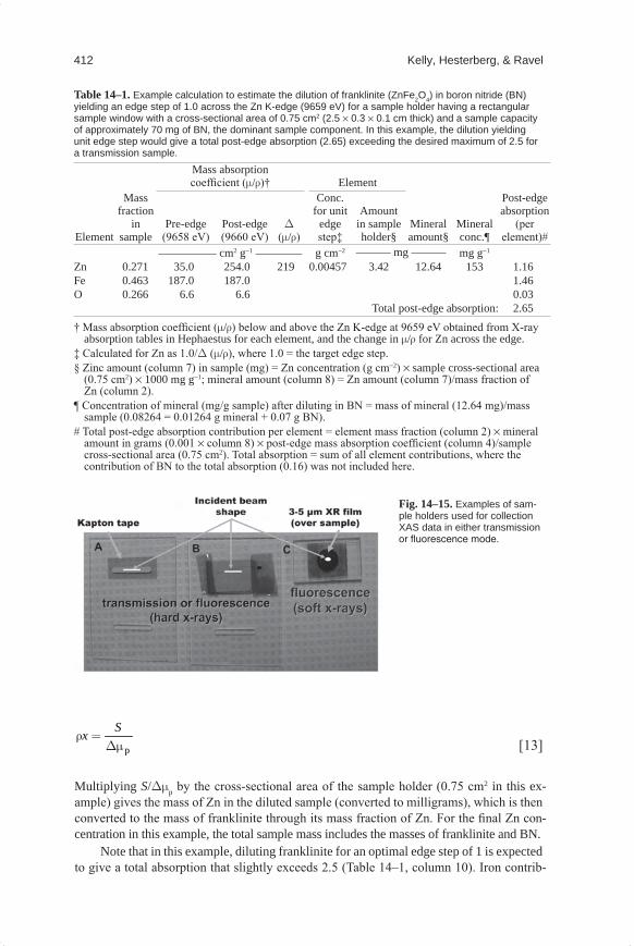
412 Kelly, Hesterberg, & Ravel
p
Sxr =Dm [13]
Multiplying S/Dmp by the cross-sectional area of the sample holder (0.75 cm2 in this ex-ample) gives the mass of Zn in the diluted sample (converted to milligrams), which is then converted to the mass of franklinite through its mass fraction of Zn. For the final Zn con-centration in this example, the total sample mass includes the masses of franklinite and BN.
Note that in this example, diluting franklinite for an optimal edge step of 1 is expected to give a total absorption that slightly exceeds 2.5 (Table 14–1, column 10). Iron contrib-
Table14–1. Example calculation to estimate the dilution of franklinite (ZnFe2O4) in boron nitride (BN) yielding an edge step of 1.0 across the Zn K-edge (9659 eV) for a sample holder having a rectangular sample window with a cross-sectional area of 0.75 cm2 (2.5 × 0.3 × 0.1 cm thick) and a sample capacity of approximately 70 mg of BN, the dominant sample component. In this example, the dilution yielding unit edge step would give a total post-edge absorption (2.65) exceeding the desired maximum of 2.5 for a transmission sample.
Element
Mass fraction
in sample
Mass absorption coefficient (m/r)† Element
Mineral amount§
Mineral conc.¶
Post-edge absorption
(per element)#
Pre-edge(9658 eV)
Post-edge(9660 eV)
D (m/r)
Conc. for unit
edge step‡
Amount in sample holder§
————— cm2 g−1 ———— g cm−2 ——— mg ——— mg g−1
Zn 0.271 35.0 254.0 219 0.00457 3.42 12.64 153 1.16Fe 0.463 187.0 187.0 1.46O 0.266 6.6 6.6 0.03
Total post-edge absorption: 2.65† Mass absorption coefficient (m/r) below and above the Zn K-edge at 9659 eV obtained from X-ray
absorption tables in Hephaestus for each element, and the change in m/r for Zn across the edge.‡ Calculated for Zn as 1.0/D (m/r), where 1.0 = the target edge step.§ Zinc amount (column 7) in sample (mg) = Zn concentration (g cm−2) × sample cross-sectional area
(0.75 cm2) × 1000 mg g−1; mineral amount (column 8) = Zn amount (column 7)/mass fraction of Zn (column 2).
¶ Concentration of mineral (mg/g sample) after diluting in BN = mass of mineral (12.64 mg)/mass sample (0.08264 = 0.01264 g mineral + 0.07 g BN).
# Total post-edge absorption contribution per element = element mass fraction (column 2) × mineral amount in grams (0.001 × column 8) × post-edge mass absorption coefficient (column 4)/sample cross-sectional area (0.75 cm2). Total absorption = sum of all element contributions, where the contribution of BN to the total absorption (0.16) was not included here.
Fig.14–15.Examples of sam-ple holders used for collection XAS data in either transmission or fluorescence mode.
Mineralogical Methods.indb 412 2/15/2008 2:37:29 PM
X-ray absorption spectroscopy 413
utes the most to the total absorption. The dilution that gives a maximum total absorption of 2.5 can be calculated from equations given in Table 14–1. Because these calculations are theoretical estimates and the BN also contributes to the total absorption (mxBN = 0.16), it is advisable to use a more conservative dilution to ensure that total absorption is < 2.5. Following the example in Table 14–1, diluting franklinite in BN to obtain a calculated edge step of 0.8 requires 0.0037 g cm−2 or 126 mg franklinite g−1 sample, giving a suitable total absorption of 2.3 (including the contribution of BN).
Sample MountingThe system used for sample mounting depends in part on the data collection mode
and the beamline end station. Samples to be collected in fluorescence mode are placed at a 45° angle with respect to the incident X-ray beam direction (Fig. 14–3B). Samples for transmission measurements can be placed perpendicular to the beam, or at a 45° angle. The amount of sample that the X-ray beam passes through will be 1.4 times greater for a sample placed at 45° angle (Fig. 14–3B) as compared with a sample placed perpendicular to the beam.
Most beamlines have a mounting bracket placed on a movable stage. The bracket is aligned in the X-ray beam so that sample holders, designed to easily attach to the mount-ing bracket, are automatically aligned in the X-ray beam. Figure 14–15 shows examples of modular sample holders. Materials such as acrylate polymer or acid-washed Teflon sheet-ing with low levels of metal impurities are suitable materials for sample holders. A window is cut completely through holders used for transmission mode data collection (Fig. 14–15A and 14–15B). If it is not possible to transmit X-rays through the sample (low-energy edges), a shallow sample well can be cut partially through the sample holder to decrease the quantity of sample needed (Fig. 14–15C). Standards diluted with a low-Z material are packed into a sample holder as shown in Fig. 14–15A. The back and front of the slot is covered with a high-purity, X-ray transparent Kapton (DuPont, Wilmington, DE) tape. Concentrated powder samples are often spread uniformly across the sticky side piece of Kapton tape (Fig. 14–15B). Care must be taken when mounting such samples to avoid pin holes. Sample thickness can be adjusted by folding the sample over to form two or more layers. As shown in Fig. 14–15B, the folded tape can be mounted directly across the window in the sample holder to assure rigidity and alignment. When working in the soft X-ray region, Kapton tape causes too much absorption. For these purposes, various types of X-ray films (e.g., mylar, polypropylene, ultralene) are available in thicknesses of 3 to 6 mm. The film is taped using Kapton across the face of the sample in a well (Fig. 14–15C).
Another option for mounting soil samples or aqueous pastes measured in transmis-sion or fluorescence mode is to place the sample in a window cut through Teflon sheeting of various thicknesses. The size of the Teflon sheeting and the location of its window are made to match the acrylate sample holder, so the Teflon mount can be taped to the holder for placement in a mounting bracket. It is often necessary to keep moist samples separated from the adhesive on the Kapton tape by first covering the sample with Kapton film.
All incident X-rays should be on a uniform region of the sample. The size of the sam-ple window or well must be larger than the dimensions of the X-ray beam and the sample must be well aligned in the X-ray beam. The beam size can be adjusted with slits with the loss of X-ray intensity. For some small, dilute samples the X-ray beam will need to be focused. Because not all beamlines have focusing capabilities, these details should be dis-cussed with the beamline scientist well before an experiment. If the X-ray beam is partially off of the sample, data quality will be poor, as described under “Thickness Effects” above.
Mineralogical Methods.indb 413 2/15/2008 2:37:29 PM
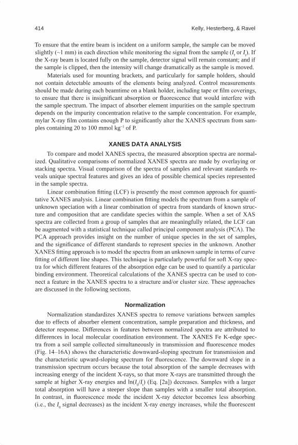
414 Kelly, Hesterberg, & Ravel
To ensure that the entire beam is incident on a uniform sample, the sample can be moved slightly (~1 mm) in each direction while monitoring the signal from the sample (If or It). If the X-ray beam is located fully on the sample, detector signal will remain constant; and if the sample is clipped, then the intensity will change dramatically as the sample is moved.
Materials used for mounting brackets, and particularly for sample holders, should not contain detectable amounts of the elements being analyzed. Control measurements should be made during each beamtime on a blank holder, including tape or film coverings, to ensure that there is insignificant absorption or fluorescence that would interfere with the sample spectrum. The impact of absorber element impurities on the sample spectrum depends on the impurity concentration relative to the sample concentration. For example, mylar X-ray film contains enough P to significantly alter the XANES spectrum from sam-ples containing 20 to 100 mmol kg−1 of P.
XANES DATA ANALYSISTo compare and model XANES spectra, the measured absorption spectra are normal-
ized. Qualitative comparisons of normalized XANES spectra are made by overlaying or stacking spectra. Visual comparison of the spectra of samples and relevant standards re-veals unique spectral features and gives an idea of possible chemical species represented in the sample spectra.
Linear combination fitting (LCF) is presently the most common approach for quanti-tative XANES analysis. Linear combination fitting models the spectrum from a sample of unknown speciation with a linear combination of spectra from standards of known struc-ture and composition that are candidate species within the sample. When a set of XAS spectra are collected from a group of samples that are meaningfully related, the LCF can be augmented with a statistical technique called principal component analysis (PCA). The PCA approach provides insight on the number of unique species in the set of samples, and the significance of different standards to represent species in the unknown. Another XANES fitting approach is to model the spectra from an unknown sample in terms of curve fitting of different line shapes. This technique is particularly powerful for soft X-ray spec-tra for which different features of the absorption edge can be used to quantify a particular binding environment. Theoretical calculations of the XANES spectra can be used to con-nect a feature in the XANES spectra to a structure and/or cluster size. These approaches are discussed in the following sections.
NormalizationNormalization standardizes XANES spectra to remove variations between samples
due to effects of absorber element concentration, sample preparation and thickness, and detector response. Differences in features between normalized spectra are attributed to differences in local molecular coordination environment. The XANES Fe K-edge spec-tra from a soil sample collected simultaneously in transmission and fluorescence modes (Fig. 14–16A) shows the characteristic downward-sloping spectrum for transmission and the characteristic upward-sloping spectrum for fluorescence. The downward slope in a transmission spectrum occurs because the total absorption of the sample decreases with increasing energy of the incident X-rays, so that more X-rays are transmitted through the sample at higher X-ray energies and ln(I0/It) (Eq. [2a]) decreases. Samples with a larger total absorption will have a steeper slope than samples with a smaller total absorption. In contrast, in fluorescence mode the incident X-ray detector becomes less absorbing (i.e., the I0 signal decreases) as the incident X-ray energy increases, while the fluorescent
Mineralogical Methods.indb 414 2/15/2008 2:37:29 PM
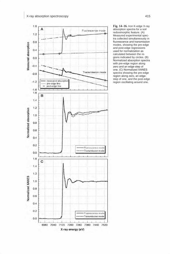
X-ray absorption spectroscopy 415
Fig.14–16.Iron K-edge X-ray absorption spectra for a soil redoximorphic feature. (A) Measured experimental spec-tra collected simultaneously in fluorescence and transmission modes, showing the pre-edge and post-edge regressions used for normalization as calculated between the re-gions indicated by circles. (B) Normalized absorption spectra with pre-edge region along zero and an edge-step of one. (C) Normalized XANES spectra showing the pre-edge region along zero, an edge-step of one, and the post-edge region oscillating around one.
Mineralogical Methods.indb 415 2/15/2008 2:37:29 PM
416 Kelly, Hesterberg, & Ravel
X-rays are at constant energy such that the fluorescence X-ray detector has the same rela-tive absorbance. As a result, the slope of If /I0 (Eq. [2b]) increases with increasing energy. Normalization removes detector (and other) effects such that normalized spectra from the same sample are identical as illustrated in Fig. 14–16C. Thus, XANES spectra for samples or standards collected in either fluorescence and transmission mode can be directly compared.
The normalization process involves a regression to the XANES spectrum in the pre-edge region (−200 to −30 eV before the edge energy) and the post-edge region (50–1000 eV above the edge energy) as delimited by the small circles in Fig. 14–16A. Usually, a linear function is regressed to the pre-edge region, and a linear or quadratic function is regressed to the post-edge region. These lines are extrapolated to the absorption edge, E0, and the difference in absorption between these projected lines at E0 is called the edge step. Normalized m(E) spectra are produced by subtracting the pre-edge line from the entire data spectrum and then dividing the spectrum by the step height. In the normalized spectrum, the pre-edge region lies along zero absorption and the edge step is 1 (Fig. 14–16B).
The post-edge region of the spectra often has a different slope or curvature than the pre-edge, such that in the normalization procedure described above, the post-edge region of the spectra will not oscillate about 1. Such spectra can be further processed by “flattening,” so the post-edge region oscillates about unit absorption. A flattening function subtracts the difference in slope between the pre- and post-edge regions and is applied only to the post-edge region above E0. The spectra in Fig. 14–16B have a non-zero slope and/or curvature that would not be removed without flattening the spectra. This flattening process does not affect the EXAFS spectra discussed below in “Edge Energy and Normalizing m(E).” The normalized and flattened spectra are called normalized XANES spectra and consist of a pre-edge region along zero absorption, a step height of one, and a post-edge region that oscillates about one as shown in Fig. 14–16C.
Sometimes, particularly in the soft X-ray energy range, XANES spectra may have inconsistent baseline and background trends, and normalization is difficult. Normalization procedures can affect the intensity of a white line and other spectral features, which conse-quently affects modeling results. A first, critical step in making an appropriate background correction for all samples and standards is the acquisition of high-quality XAS data. It is a good practice to collect data for normalizing XAS spectra across a broad energy range ex-tending well above the absorption edge (>200 eV) where EXAFS oscillations are weaker. Large (5–10 eV) steps can be taken across this region if only XANES data are being col-lected. It is also important that a normalization procedure be applied consistently between samples and standards (Sayers and Bunker, 1988).
Linear Combination FittingThe underlying principle of linear combination fitting (LCF) is the additive nature of
the absorption from each species in the sample. It can be applied to XANES, derivative XANES, or EXAFS spectra. As shown in Eq. [12] the total absorption coefficient can be written as a sum of coefficients for all the elements in the sample. It can also be written as a sum of chemical forms or species. For example, if a sample contains 50% goethite and 50% ferrihydrite, the absorption coefficient can be written as a weighted sum of the absorption coefficients for goethite and ferrihydrite, where each of these species has a contribution from Fe, O, and H atoms. As such, LCF involves modeling the spectrum for a sample of unknown chemical speciation using spectra from representative standards.
Linear combination fitting subroutines are available in XAS data analysis programs like Athena (Ravel and Newville, 2005) and Sixpack (Webb, 2007). These programs
Mineralogical Methods.indb 416 2/15/2008 2:37:29 PM
X-ray absorption spectroscopy 417
compute the scaling factors applied to different standard spectra that provide the best rep-resentation of the measured spectrum over a defined energy range. Mathematically,
( )Model STDi ii
f=å [14]
where Model represents the least-squares fit to the sample spectrum over a selected energy range, and fi represents the scaling factors applied to each spectrum of the corresponding standard (STDi) across that energy range of the fit. It is good practice for all spectra includ-ed in the LCF to have a similar energy resolution. Consistent normalization is important for LCF. To test for and possibly account for normalization problems, a line can be added into the fit as a standard. The statistical goodness-of-fit parameters for LCF are similar to those described for EXAFS analysis in the section “Comparing Models Using Statistical Tools” below.
Number of StandardsThe number of standards included in a XANES LCF depends on the complexity of
the chemical system. For example, only two standards would be used to characterize the XANES spectrum for a well-defined chemical system that, based on the known chemical composition, is likely to contain only two chemical species. For complex systems like soils that might contain many species, the number of standards would be limited to the number of species to which the XANES spectrum is sensitive, and caution should be used to avoid overfitting the spectrum with too many standards. For example, Beauchemin et al. (2003) identified the main forms of inorganic phosphate in soil samples. However, each of several possible forms of organic P present in most soils could not be differentiated be-cause each form would likely occur at <10 mol% in the sample, and some of these species have XANES spectra with broad nondistinct features. Statistical methods, such as PCA, are helpful in determining the number of possible species within an unknown sample, al-though this method has many of the same limitations as LCF.
Fitting RangeThe energy range for fitting an XAS spectrum using LCF is flexible, provided that
data over that range are available for both samples and standards. Because the dominant feature in a XANES spectrum is the white line, this feature will have the most influence on a XANES fitting result. Therefore, LCF is particularly sensitive to various chemical species when each species gives unique features in the white-line region. However, for a particular problem, it might be desirable to isolate a specific, unique feature that can be used to differentiate between two or more different bonding environments of the absorber element. For example, Khare et al. (2004, 2005) used LCF fitting of a feature unique to Fe(III)-bonded phosphate to quantify the relative amounts of phosphate bound to Fe(III) oxide vs. Al(III) oxide in mineral mixtures. Murray and Hesterberg (2006) performed the same analysis to quantify the proportion of Fe(III)-bonded phosphate in mineral mixtures that underwent abiotic reduction, but they additionally performed LCF across the white line to establish whether the Al(III)-bonded phosphate was more likely adsorbed or pre-cipitated as Al phosphate.
When analyzing soil samples that likely contain multiple forms of unknown chemical species, it is best to visually compare the spectra for samples and standards to determine the energy range that captures unique features of each standard. Then, begin the fitting over this energy range, and refine the energy range as insights are gained about the dominant chemical species present.
Mineralogical Methods.indb 417 2/15/2008 2:37:30 PM
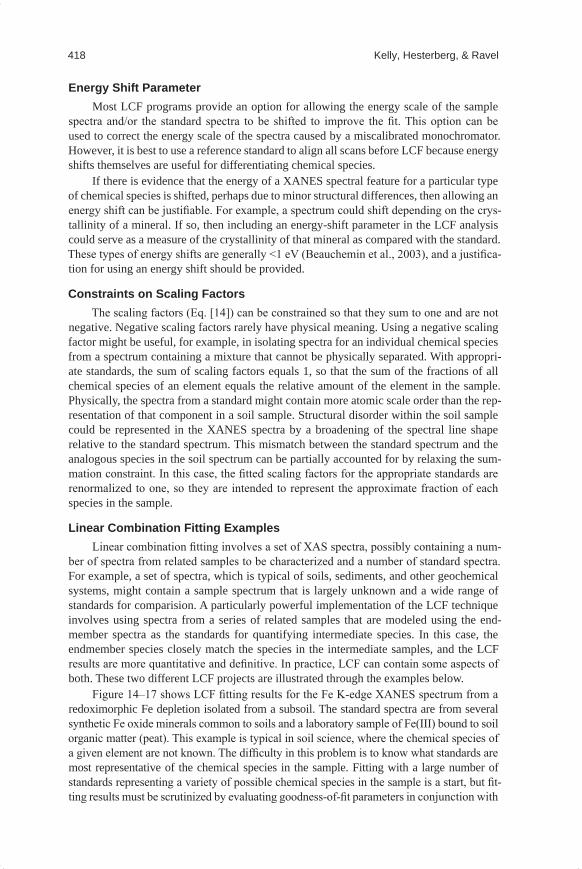
418 Kelly, Hesterberg, & Ravel
Energy Shift ParameterMost LCF programs provide an option for allowing the energy scale of the sample
spectra and/or the standard spectra to be shifted to improve the fit. This option can be used to correct the energy scale of the spectra caused by a miscalibrated monochromator. However, it is best to use a reference standard to align all scans before LCF because energy shifts themselves are useful for differentiating chemical species.
If there is evidence that the energy of a XANES spectral feature for a particular type of chemical species is shifted, perhaps due to minor structural differences, then allowing an energy shift can be justifiable. For example, a spectrum could shift depending on the crys-tallinity of a mineral. If so, then including an energy-shift parameter in the LCF analysis could serve as a measure of the crystallinity of that mineral as compared with the standard. These types of energy shifts are generally <1 eV (Beauchemin et al., 2003), and a justifica-tion for using an energy shift should be provided.
Constraints on Scaling FactorsThe scaling factors (Eq. [14]) can be constrained so that they sum to one and are not
negative. Negative scaling factors rarely have physical meaning. Using a negative scaling factor might be useful, for example, in isolating spectra for an individual chemical species from a spectrum containing a mixture that cannot be physically separated. With appropri-ate standards, the sum of scaling factors equals 1, so that the sum of the fractions of all chemical species of an element equals the relative amount of the element in the sample. Physically, the spectra from a standard might contain more atomic scale order than the rep-resentation of that component in a soil sample. Structural disorder within the soil sample could be represented in the XANES spectra by a broadening of the spectral line shape relative to the standard spectrum. This mismatch between the standard spectrum and the analogous species in the soil spectrum can be partially accounted for by relaxing the sum-mation constraint. In this case, the fitted scaling factors for the appropriate standards are renormalized to one, so they are intended to represent the approximate fraction of each species in the sample.
Linear Combination Fitting ExamplesLinear combination fitting involves a set of XAS spectra, possibly containing a num-
ber of spectra from related samples to be characterized and a number of standard spectra. For example, a set of spectra, which is typical of soils, sediments, and other geochemical systems, might contain a sample spectrum that is largely unknown and a wide range of standards for comparision. A particularly powerful implementation of the LCF technique involves using spectra from a series of related samples that are modeled using the end-member spectra as the standards for quantifying intermediate species. In this case, the endmember species closely match the species in the intermediate samples, and the LCF results are more quantitative and definitive. In practice, LCF can contain some aspects of both. These two different LCF projects are illustrated through the examples below.
Figure 14–17 shows LCF fitting results for the Fe K-edge XANES spectrum from a redoximorphic Fe depletion isolated from a subsoil. The standard spectra are from several synthetic Fe oxide minerals common to soils and a laboratory sample of Fe(III) bound to soil organic matter (peat). This example is typical in soil science, where the chemical species of a given element are not known. The difficulty in this problem is to know what standards are most representative of the chemical species in the sample. Fitting with a large number of standards representing a variety of possible chemical species in the sample is a start, but fit-ting results must be scrutinized by evaluating goodness-of-fit parameters in conjunction with
Mineralogical Methods.indb 418 2/15/2008 2:37:30 PM
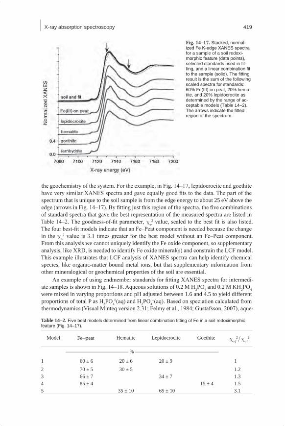
X-ray absorption spectroscopy 419
the geochemistry of the system. For the example, in Fig. 14–17, lepidocrocite and goethite have very similar XANES spectra and gave equally good fits to the data. The part of the spectrum that is unique to the soil sample is from the edge energy to about 25 eV above the edge (arrows in Fig. 14–17). By fitting just this region of the spectra, the five combinations of standard spectra that gave the best representation of the measured spectra are listed in Table 14–2. The goodness-of-fit parameter, cn
2 value, scaled to the best fit is also listed. The four best-fit models indicate that an Fe–Peat component is needed because the change in the cn
2 value is 3.1 times greater for the best model without an Fe–Peat component. From this analysis we cannot uniquely identify the Fe oxide component, so supplementary analysis, like XRD, is needed to identify Fe oxide mineral(s) and constrain the LCF model. This example illustrates that LCF analysis of XANES spectra can help identify chemical species, like organic-matter bound metal ions, but that supplementary information from other mineralogical or geochemical properties of the soil are essential.
An example of using endmember standards for fitting XANES spectra for intermedi-ate samples is shown in Fig. 14–18. Aqueous solutions of 0.2 M H3PO4 and 0.2 M KH2PO4 were mixed in varying proportions and pH adjusted between 1.6 and 4.5 to yield different proportions of total P as H3PO4
0(aq) and H2PO4−(aq). Based on speciation calculated from
thermodynamics (Visual Minteq version 2.31; Felmy et al., 1984; Gustafsson, 2007), aque-
Fig. 14–17. Stacked, normal-ized Fe K-edge XANES spectra for a sample of a soil redoxi-morphic feature (data points), selected standards used in fit-ting, and a linear combination fit to the sample (solid). The fitting result is the sum of the following scaled spectra for standards: 60% Fe(III) on peat, 20% hema-tite, and 20% lepidocrocite as determined by the range of ac-ceptable models (Table 14–2). The arrows indicate the fitted region of the spectrum.
Table14–2. Five best models determined from linear combination fitting of Fe in a soil redoximorphic feature (Fig. 14–17).
Model Fe–peat Hematite Lepidocrocite Goethite cnf2/cni
2
———————————— % ————————————————
1 60 ± 6 20 ± 6 20 ± 9 12 70 ± 5 30 ± 5 1.23 66 ± 7 34 ± 7 1.34 85 ± 4 15 ± 4 1.55 35 ± 10 65 ± 10 3.1
Mineralogical Methods.indb 419 2/15/2008 2:37:30 PM
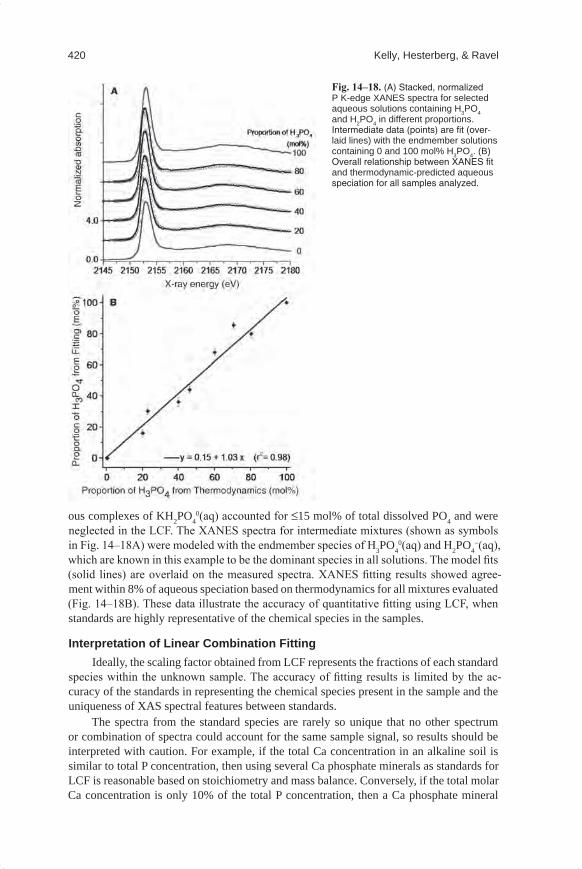
420 Kelly, Hesterberg, & Ravel
ous complexes of KH2PO40(aq) accounted for ≤15 mol% of total dissolved PO4 and were
neglected in the LCF. The XANES spectra for intermediate mixtures (shown as symbols in Fig. 14–18A) were modeled with the endmember species of H3PO4
0(aq) and H2PO4−(aq),
which are known in this example to be the dominant species in all solutions. The model fits (solid lines) are overlaid on the measured spectra. XANES fitting results showed agree-ment within 8% of aqueous speciation based on thermodynamics for all mixtures evaluated (Fig. 14–18B). These data illustrate the accuracy of quantitative fitting using LCF, when standards are highly representative of the chemical species in the samples.
Interpretation of Linear Combination FittingIdeally, the scaling factor obtained from LCF represents the fractions of each standard
species within the unknown sample. The accuracy of fitting results is limited by the ac-curacy of the standards in representing the chemical species present in the sample and the uniqueness of XAS spectral features between standards.
The spectra from the standard species are rarely so unique that no other spectrum or combination of spectra could account for the same sample signal, so results should be interpreted with caution. For example, if the total Ca concentration in an alkaline soil is similar to total P concentration, then using several Ca phosphate minerals as standards for LCF is reasonable based on stoichiometry and mass balance. Conversely, if the total molar Ca concentration is only 10% of the total P concentration, then a Ca phosphate mineral
Fig. 14–18. (A) Stacked, normalized P K-edge XANES spectra for selected aqueous solutions containing H3PO4 and H2PO4 in different proportions. Intermediate data (points) are fit (over-laid lines) with the endmember solutions containing 0 and 100 mol% H3PO4. (B) Overall relationship between XANES fit and thermodynamic-predicted aqueous speciation for all samples analyzed.
Mineralogical Methods.indb 420 2/15/2008 2:37:31 PM
X-ray absorption spectroscopy 421
like CaH2PO4 having a 1:1 Ca/P ratio can be included in the LCF only up to 10 mol%. If the model assigns more than 10% of total P as CaH2PO4, the result is chemically impos-sible, indicating that there must be another species within the soil that has a spectrum similar to CaH2PO4. Often more than one combination of standards gives similar quality of fit (Beauchemin et al., 2003), which is attributable to an insensitivity of LCF analysis to different chemical species. Additional geochemical information is needed to evaluate the degree to which the standards represent species within a sample.
It cannot be overemphasized that minerals and other solid-phase chemical species in soils and other natural systems have compositions along a continuum (e.g., different levels of impurities or a range of crystallinities), making it unlikely that the exact distribution of unknown species in a natural sample can be simulated using pure standards. A reasonable model based on LCF does not prove that these standards are the exact chemical species in the soil. Rather, LCF results identify the proportions of standards that yield the best fit to the data, recognizing that if a more representative set of standards are identified, then the accuracy of the results improves.
Principal Component AnalysisThe principal component analysis (PCA) approach provides insight on the number of
unique components present in a set of samples, and the likelihood that a standard represents a species in the samples via target transformations. This approach is commonly combined with LCF to help determine the number of standard spectra and to define the standard spec-tra. Principal component analysis is used with a set of spectra that are meaningfully related, such as soils exposed to different chemical treatments or soil samples along a geochemical gradient that naturally vary in the speciation of the absorber element. Research has shown that the number of components obtained statistically by applying PCA to XANES datasets for P in soils, S in humic acid, and Mn in airborne particulates ranged from two to three (Ressler et al., 2000; Beauchemin et al., 2002; 2003). Additional examples of PCA applied to XANES or EXAFS spectra can be found in Fernández-García et al. (1995); Wasserman (1997), and Wasserman et al. (1999). Details of the theory and practice of PCA in chemical systems are given in Malinowski (2002), and the PCA approach for S XANES spectra is described in some detail by Beauchemin et al. (2002).
Principal component analysis uses matrix operations to determine eigenvectors that represent the variation in the set of spectra. The maximum number of eigenvectors is equal to the number of sample spectra. The first eigenvector is defined as a vector along the great-est variation in some aspect of the data set. The second vector is extracted orthogonally to the first one to account for the highest remaining variation. Additional eigenvectors are orthogonally extracted until all the variation in the dataset is captured. There are several criteria that can be used to statistically separate the significant eigenvectors from those rep-resenting noise in the data set. The significant eigenvectors are called principle components and are statistical abstractions with no physical relationship to the chemical components or species in the samples.
Ideally, the number of significant components would be equal to the number of chemical species in the sample, thereby constraining the maximum number of standards that should be combined to model a given sample spectrum. In practice, the number of significant components is not necessarily equal to the number of different chemical spe-cies contained within the set of samples because the chemical species are not necessarily unique. For example, if two different species are always present in the same fraction within each spectrum of the data set, then these two species will be represented by a single prin-
Mineralogical Methods.indb 421 2/15/2008 2:37:31 PM
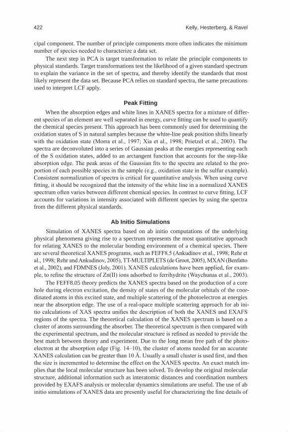
422 Kelly, Hesterberg, & Ravel
cipal component. The number of principle components more often indicates the minimum number of species needed to characterize a data set.
The next step in PCA is target transformation to relate the principle components to physical standards. Target transformations test the likelihood of a given standard spectrum to explain the variance in the set of spectra, and thereby identify the standards that most likely represent the data set. Because PCA relies on standard spectra, the same precautions used to interpret LCF apply.
Peak FittingWhen the absorption edges and white lines in XANES spectra for a mixture of differ-
ent species of an element are well separated in energy, curve fitting can be used to quantify the chemical species present. This approach has been commonly used for determining the oxidation states of S in natural samples because the white-line peak position shifts linearly with the oxidation state (Morra et al., 1997; Xia et al., 1998; Prietzel et al., 2003). The spectra are deconvoluted into a series of Gaussian peaks at the energies representing each of the S oxidation states, added to an arctangent function that accounts for the step-like absorption edge. The peak areas of the Gaussian fits to the spectra are related to the pro-portion of each possible species in the sample (e.g., oxidation state in the sulfur example). Consistent normalization of spectra is critical for quantitative analysis. When using curve fitting, it should be recognized that the intensity of the white line in a normalized XANES spectrum often varies between different chemical species. In contrast to curve fitting, LCF accounts for variations in intensity associated with different species by using the spectra from the different physical standards.
Ab Initio SimulationsSimulation of XANES spectra based on ab initio computations of the underlying
physical phenomena giving rise to a spectrum represents the most quantitative approach for relating XANES to the molecular bonding environment of a chemical species. There are several theoretical XANES programs, such as FEFF8.5 (Ankudinov et al., 1998; Rehr et al., 1998; Rehr and Ankudinov, 2005), TT-MULTIPLETS (de Groot, 2005), MXAN (Benfatto et al., 2002), and FDMNES (Joly, 2001). XANES calculations have been applied, for exam-ple, to refine the structure of Zn(II) ions adsorbed to ferrihydrite (Waychunas et al., 2003).
The FEFF8.05 theory predicts the XANES spectra based on the production of a core hole during electron excitation, the density of states of the molecular orbitals of the coor-dinated atoms in this excited state, and multiple scattering of the photoelectron at energies near the absorption edge. The use of a real-space multiple scattering approach for ab ini-tio calculations of XAS spectra unifies the description of both the XANES and EXAFS regions of the spectra. The theoretical calculation of the XANES spectrum is based on a cluster of atoms surrounding the absorber. The theoretical spectrum is then compared with the experimental spectrum, and the molecular structure is refined as needed to provide the best match between theory and experiment. Due to the long mean free path of the photo-electron at the absorption edge (Fig. 14–10), the cluster of atoms needed for an accurate XANES calculation can be greater than 10 Å. Usually a small cluster is used first, and then the size is incremented to determine the effect on the XANES spectra. An exact match im-plies that the local molecular structure has been solved. To develop the original molecular structure, additional information such as interatomic distances and coordination numbers provided by EXAFS analysis or molecular dynamics simulations are useful. The use of ab initio simulations of XANES data are presently useful for characterizing the fine details of
Mineralogical Methods.indb 422 2/15/2008 2:37:31 PM
X-ray absorption spectroscopy 423
a structure of a given mineral or adsorbed species, and it could potentially become useful for characterizing multicomponent systems like soils.
X-RAY ABSORPTION FINE STRUCTURE DATA ANALYSISThe objective of EXAFS data analysis is to develop a structural model of atoms co-
ordinated to the absorber atoms, as a means of identifying the chemical form(s) of the absorber. Interpreting the structural information contained in EXAFS spectra requires knowledge of spectroscopy, a basic understanding of signal processing and Fourier trans-forms, and knowledge of the fundamental processes that generate the EXAFS signal.
In the following sections, we present the details of how EXAFS spectra are processed and modeled in terms of local molecular coordination. We describe EXAFS spectral pro-cessing, building theoretical models, and examples of theoretical modeling.
The “EXAFS Data Processing” section includes preprocessing of XAS spectra, operations performed on the spectra as measured in energy, the basics of Fourier trans-formations, and background removal procedures for isolating the oscillatory part of the absorption coefficient.
The description of building theoretical models includes an overview of the basic com-ponents, the basics of constructing the theoretical EXAFS spectra using FEFF, common methods for constraining EXAFS parameters, the fundamentals of building an EXAFS model, and comparing models using statistical tools.
The EXAFS modeling examples include aligning the data and theory in energy, modeling a metal-oxide (SnO2), determining a second shell atom type, and modeling a data series.
This section is concluded with tips for reporting EXAFS analysis in published manu-scripts and some final concluding remarks. In our descriptions, reference is made to the Athena and Artemis software packages for EXAFS data analysis (Ravel and Newville, 2005). A number of other software packages are available for EXAFS data analysis, and information about many of these programs can be found at www.xafs.org/Software (veri-fied 20 Dec. 2007).
EXAFS DATA ProcessingThere are several data processing steps that may be needed to refine the final spectrum
for analysis. These preprocessing procedures include rebinning measured data points, re-moval of data points that are clearly in error (deglitching), trimming the absorption spectra to the usable energy region (truncation), changing the energy scale to align several scans, and averaging several scans to produce a high quality spectrum for analysis.
RebinningDepending on the energy spacing of XAS data points, the signal/noise ratio may be in-
creased by averaging the signal from closely spaced energy points to obtain a single value at an average energy. This procedure is called rebinning. The above section “XAS Scan Parameters” gives the detailed energy resolution requirements for an XAS scan. Rebinning is particularly useful for spectra collected in quick-scanning mode of the monochromator to produce evenly spaced energy points.
Glitch RemovalAt certain energies for a given monochromator crystal, the crystal geometry is such
that the primary diffracted beam undergoes a second diffraction from a different set of
Mineralogical Methods.indb 423 2/15/2008 2:37:31 PM
424 Kelly, Hesterberg, & Ravel
atomic planes, resulting in the loss of X-ray intensity going to the sample (Heald, 1988b). The sharp drop in the incident X-ray intensity (I0) can cause a spike or dip in the XAS spec-trum. These points are called monochromator glitches. With very good linear response of the detectors, glitches are cancelled out in the ratio of the detector signals (Eq. [2]), such that the absorption spectra, m(E), are unaffected. In some cases, glitches can be avoided by adjusting the beamline optics (e.g., changing the detuning or rotating the crystals laterally or normally to change the region of the crystals reflecting the X-rays). When a glitch persists in the EXAFS spectra, these points can be removed. If glitches contribute to the data structure, then they will distort the background or cause artifacts in the EXAFS spectrum that can affect the final fitting results. These problems can be easily avoided by careful analysis procedures.
One method for determining the significance of a glitch is to remove the background with and without including the data points from the glitch to determine the effect on the EXAFS signal. As with rebinning, often an EXAFS spectrum is oversampled in energy so that the loss of a few data points to remove a glitch will not significantly decrease the in-formation content in the measured spectrum. Caution should be used when omitting glitch points when it results in a loss in energy points corresponding to a radial distance (R) < 10 Å. This requires that the remaining data points are not separated by more than 0.16 Å−1 in k, determined by the relation R = p/(2Dk). For example, if the data are collected with a 0.05 Å−1 spacing in k, then three consecutive data points can be removed with tolerable loss of information.
TruncatingDramatic changes in the X-ray absorption coefficient before or after the absorption
edge should not be included in the final spectrum for analysis. These features can produce errors when determining the step height or in the background removal procedures. Possible causes for such a dramatic change in the absorption coefficient include an absorption edge from another element or beamline-specific energy-dependent structure. For example, Fig. 14–19A shows the U LIII–edge at 17,166 eV with a pre-edge region that has been obscured by the yttrium K-edge at 17,038 eV. The region of the data that contains the smooth, step-like absorption edge should be isolated from the interfering region by removing data points affected by the Y K-edge, or by adjusting the ranges used to process the data so that the unwanted feature is excluded. The pre-edge region from 16,900 to 17,100 eV (−200 to −50 eV relative to the edge energy) in Fig. 14–19A results in a steep, positively sloped pre-edge line that is clearly not along the baseline (gray line). A more correct pre-edge line would be the line with a negative slope obtained by using the very short data range just before the U edge, from 17,090 to 17,120 eV. Effects of each pre-edge line on the XAS spectrum are shown in Fig. 14–19 B–D and are discussed in more detail below
Aligning and Averaging SpectraThe edge energy of the spectrum from the reference standard can be used to define the
absolute energy scale for the measured sample spectra. Shifts in energy during data collec-tion can be caused by mechanical instabilities in the monochromator, such as a missed step of the monochromator motor used to change the energy or changes in the monochromator temperature due to heat load differences between synchrotron ring fills.
Because multiple scans are usually collected from a single sample, the resulting m(E) spectra should be aligned to a common energy scale to avoid loss of energy resolution, then averaged to increase the signal/noise ratio in the final spectrum. Alignment of spectra to an absolute energy scale is important for XANES data analysis, whereas it is sufficient for EXAFS analysis to align spectra to a common, relative energy scale.
Mineralogical Methods.indb 424 2/15/2008 2:37:31 PM
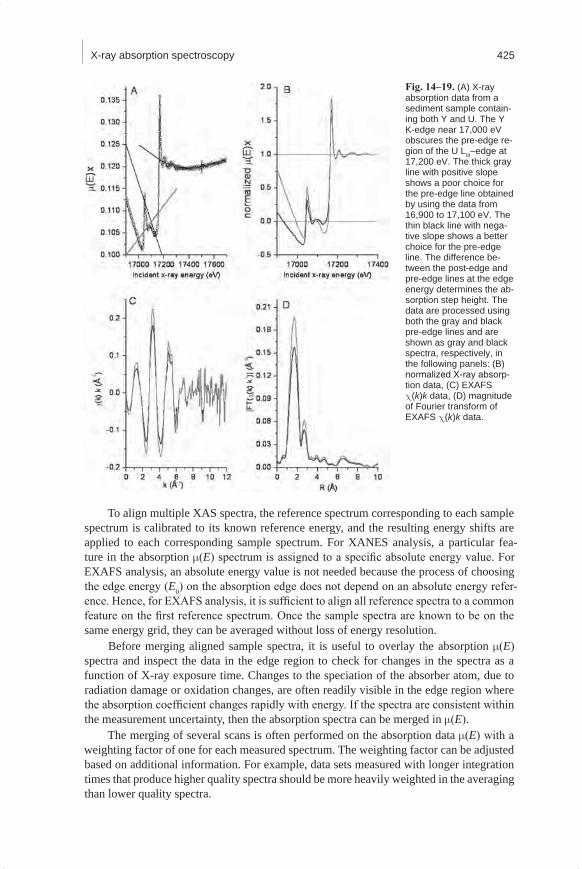
X-ray absorption spectroscopy 425
To align multiple XAS spectra, the reference spectrum corresponding to each sample spectrum is calibrated to its known reference energy, and the resulting energy shifts are applied to each corresponding sample spectrum. For XANES analysis, a particular fea-ture in the absorption m(E) spectrum is assigned to a specific absolute energy value. For EXAFS analysis, an absolute energy value is not needed because the process of choosing the edge energy (E0) on the absorption edge does not depend on an absolute energy refer-ence. Hence, for EXAFS analysis, it is sufficient to align all reference spectra to a common feature on the first reference spectrum. Once the sample spectra are known to be on the same energy grid, they can be averaged without loss of energy resolution.
Before merging aligned sample spectra, it is useful to overlay the absorption m(E) spectra and inspect the data in the edge region to check for changes in the spectra as a function of X-ray exposure time. Changes to the speciation of the absorber atom, due to radiation damage or oxidation changes, are often readily visible in the edge region where the absorption coefficient changes rapidly with energy. If the spectra are consistent within the measurement uncertainty, then the absorption spectra can be merged in m(E).
The merging of several scans is often performed on the absorption data m(E) with a weighting factor of one for each measured spectrum. The weighting factor can be adjusted based on additional information. For example, data sets measured with longer integration times that produce higher quality spectra should be more heavily weighted in the averaging than lower quality spectra.
Fig. 14–19. (A) X-ray absorption data from a sediment sample contain-ing both Y and U. The Y K-edge near 17,000 eV obscures the pre-edge re-gion of the U LIII–edge at 17,200 eV. The thick gray line with positive slope shows a poor choice for the pre-edge line obtained by using the data from 16,900 to 17,100 eV. The thin black line with nega-tive slope shows a better choice for the pre-edge line. The difference be-tween the post-edge and pre-edge lines at the edge energy determines the ab-sorption step height. The data are processed using both the gray and black pre-edge lines and are shown as gray and black spectra, respectively, in the following panels: (B) normalized X-ray absorp-tion data, (C) EXAFS c(k)k data, (D) magnitude of Fourier transform of EXAFS c(k)k data.
Mineralogical Methods.indb 425 2/15/2008 2:37:32 PM
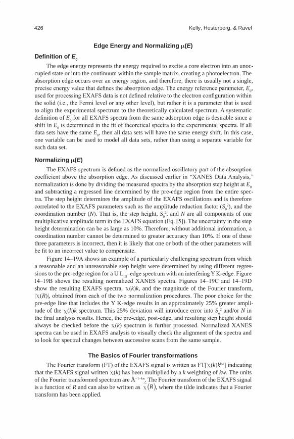
426 Kelly, Hesterberg, & Ravel
Edge Energy and Normalizing m(E)
Definition of E0
The edge energy represents the energy required to excite a core electron into an unoc-cupied state or into the continuum within the sample matrix, creating a photoelectron. The absorption edge occurs over an energy region, and therefore, there is usually not a single, precise energy value that defines the absorption edge. The energy reference parameter, E0, used for processing EXAFS data is not defined relative to the electron configuration within the solid (i.e., the Fermi level or any other level), but rather it is a parameter that is used to align the experimental spectrum to the theoretically calculated spectrum. A systematic definition of E0 for all EXAFS spectra from the same adsorption edge is desirable since a shift in E0 is determined in the fit of theoretical spectra to the experimental spectra. If all data sets have the same E0, then all data sets will have the same energy shift. In this case, one variable can be used to model all data sets, rather than using a separate variable for each data set.
Normalizing m(E)The EXAFS spectrum is defined as the normalized oscillatory part of the absorption
coefficient above the absorption edge. As discussed earlier in “XANES Data Analysis,” normalization is done by dividing the measured spectra by the absorption step height at E0 and subtracting a regressed line determined by the pre-edge region from the entire spec-tra. The step height determines the amplitude of the EXAFS oscillations and is therefore correlated to the EXAFS parameters such as the amplitude reduction factor (S0
2), and the coordination number (N). That is, the step height, S0
2, and N are all components of one multiplicative amplitude term in the EXAFS equation (Eq. [5]). The uncertainty in the step height determination can be as large as 10%. Therefore, without additional information, a coordination number cannot be determined to greater accuracy than 10%. If one of these three parameters is incorrect, then it is likely that one or both of the other parameters will be fit to an incorrect value to compensate.
Figure 14–19A shows an example of a particularly challenging spectrum from which a reasonable and an unreasonable step height were determined by using different regres-sions to the pre-edge region for a U LIII–edge spectrum with an interfering Y K-edge. Figure 14–19B shows the resulting normalized XANES spectra. Figures 14–19C and 14–19D show the resulting EXAFS spectra, c(k)k, and the magnitude of the Fourier transform, |c(R)|, obtained from each of the two normalization procedures. The poor choice for the pre-edge line that includes the Y K-edge results in an approximately 25% greater ampli-tude of the c(k)k spectrum. This 25% deviation will introduce error into So
2 and/or N in the final analysis results. Hence, the pre-edge, post-edge, and resulting step height should always be checked before the c(k) spectrum is further processed. Normalized XANES spectra can be used in EXAFS analysis to visually check the alignment of the spectra and to look for spectral changes between successive scans from the same sample.
The Basics of Fourier transformationsThe Fourier transform (FT) of the EXAFS signal is written as FT[c(k)kkw] indicating
that the EXAFS signal written c(k) has been multiplied by a k weighting of kw. The units of the Fourier transformed spectrum are Å−1−kw. The Fourier transform of the EXAFS signal is a function of R and can also be written as ( )Rc , where the tilde indicates that a Fourier transform has been applied.
Mineralogical Methods.indb 426 2/15/2008 2:37:32 PM
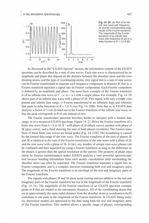
X-ray absorption spectroscopy 427
As discussed in the “EXAFS Spectra” section, the information content of the EXAFS spectrum can be described by a sum of sine waves. Each sine wave is characterized by an amplitude and phase that depend on the distance between the absorber atom and the coor-dinating atoms, and the type of coordinating atoms. Any signal that is a sum of sine waves can be Fourier transformed to separate each frequency component in distance R; that is, a Fourier transform separates a signal into its Fourier components. Each Fourier component is defined by an amplitude and phase. The most basic example of the Fourier transform is of an infinite sine wave (k = −¥ to +¥) with a single phase. For example, Fig. 14–20 shows part of an infinite sine wave with a phase of 2k. This signal, with only a single com-ponent and infinite data range, is Fourier transformed to an infinitely high and infinitely thin peak (a delta function) at R = 1.0 Å (see Fig. 14–20B). Note that as in EXAFS data analysis, a factor of 2 was divided out in the Fourier transform of the infinite sine wave, so that the peak corresponds to R of one instead of two.
The Fourier transformed spectrum becomes harder to interpret with a limited data range, as in a measured EXAFS spectrum. Figure 14–21 shows the Fourier transform of a finite sine wave from k = 0 to 10 Å−1 with phase of 2k (black curve), another with phase of 3k (gray curve), and a third showing the sum of both phases (symbols). The Fourier trans-form of these finite sine waves are broad peaks (Fig. 14–21B). The broadening is caused by the limited data range of the sine wave. The Fourier transform of the sum of phases 2k and 3k is identical to the sum of the Fourier transforms of the sine wave with a phase of 2k and the sine wave with a phase of 3k. In fact, any number of unique sine-wave phases can be combined and then separated by using a Fourier transform as long as the difference in the phases is greater than the spatial resolution of the spectra. The property of phase sepa-ration by Fourier transformation makes EXAFS analysis a very powerful spectroscopic tool because bonding information from each atomic coordination shell surrounding the absorber atom can often be separated. The Fourier transform separates a signal into its Fourier components and is a complex function containing both real and imaginary parts. The magnitude of the Fourier transform is an envelope of the real and imaginary parts of the Fourier transform.
The signals with phases 2k and 3k show some overlap and are additive in the real and imaginary parts of the Fourier transform but not in the magnitude of the Fourier transform (Fig. 14–21). The magnitude of the Fourier transform of an EXAFS spectrum contains peaks in R that are related to the interatomic distances. All of the coordinating atoms that are at approximately the same radial distance from the absorber atom (a coordination shell) contribute to one peak in the magnitude of the Fourier transform. In EXAFS fitting analy-sis, theoretical models are optimized to the data using both the real and imaginary parts of the Fourier transform. This method allows a specific range of phases, corresponding
Fig.14–20. (A) Part of an infi-nite sine wave with frequency 2k and (B) corresponding mag-nitude of the Fourier transform. The magnitude of the Fourier transform of an infinite sine wave with frequency 2k (A) is a delta function at R = 1.0 Å (B).
Mineralogical Methods.indb 427 2/15/2008 2:37:33 PM
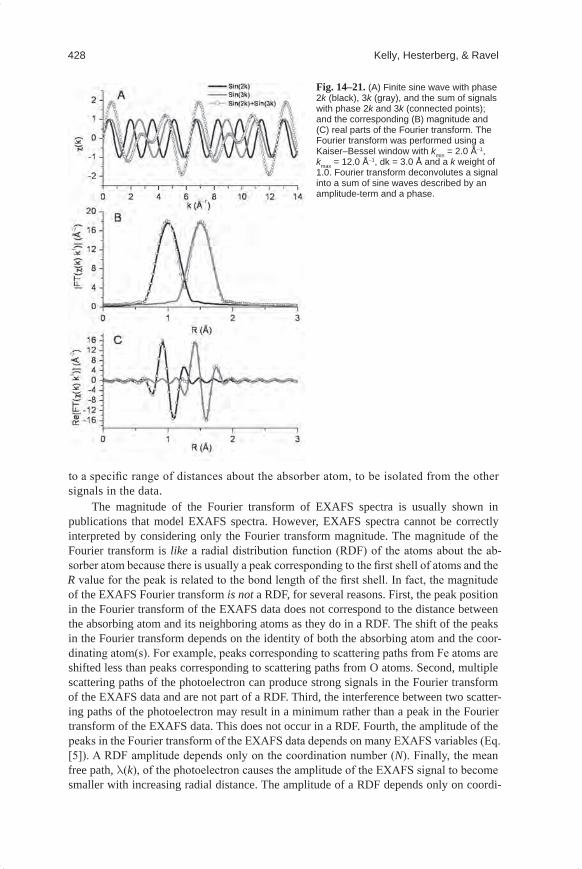
428 Kelly, Hesterberg, & Ravel
to a specific range of distances about the absorber atom, to be isolated from the other signals in the data.
The magnitude of the Fourier transform of EXAFS spectra is usually shown in publications that model EXAFS spectra. However, EXAFS spectra cannot be correctly interpreted by considering only the Fourier transform magnitude. The magnitude of the Fourier transform is like a radial distribution function (RDF) of the atoms about the ab-sorber atom because there is usually a peak corresponding to the first shell of atoms and the R value for the peak is related to the bond length of the first shell. In fact, the magnitude of the EXAFS Fourier transform is not a RDF, for several reasons. First, the peak position in the Fourier transform of the EXAFS data does not correspond to the distance between the absorbing atom and its neighboring atoms as they do in a RDF. The shift of the peaks in the Fourier transform depends on the identity of both the absorbing atom and the coor-dinating atom(s). For example, peaks corresponding to scattering paths from Fe atoms are shifted less than peaks corresponding to scattering paths from O atoms. Second, multiple scattering paths of the photoelectron can produce strong signals in the Fourier transform of the EXAFS data and are not part of a RDF. Third, the interference between two scatter-ing paths of the photoelectron may result in a minimum rather than a peak in the Fourier transform of the EXAFS data. This does not occur in a RDF. Fourth, the amplitude of the peaks in the Fourier transform of the EXAFS data depends on many EXAFS variables (Eq. [5]). A RDF amplitude depends only on the coordination number (N). Finally, the mean free path, l(k), of the photoelectron causes the amplitude of the EXAFS signal to become smaller with increasing radial distance. The amplitude of a RDF depends only on coordi-
Fig.14–21. (A) Finite sine wave with phase 2k (black), 3k (gray), and the sum of signals with phase 2k and 3k (connected points); and the corresponding (B) magnitude and (C) real parts of the Fourier transform. The Fourier transform was performed using a Kaiser–Bessel window with kmin = 2.0 Å−1, kmax = 12.0 Å−1, dk = 3.0 Å and a k weight of 1.0. Fourier transform deconvolutes a signal into a sum of sine waves described by an amplitude-term and a phase.
Mineralogical Methods.indb 428 2/15/2008 2:37:34 PM
X-ray absorption spectroscopy 429
nation number. In essence, the magnitude of the Fourier transform of the EXAFS data is a complicated signal that depends only in part on the RDF.
Information Content of a Fourier Transformed SpectrumThe EXAFS signal is a sum of sine waves with an amplitude that depends on wave-
number k. To analyze these sine waves in terms of atomic coordination, the EXAFS spectrum is Fourier transformed. Information theory is used to correlate the amount of information in the original EXAFS spectrum to the information in Fourier transform spec-trum as determined from the Nyquist theorem
IP2 1N = k R +D Dp
[15]
where NIP is the number of independent points, Dk is the Fourier transformed data range and DR is the region used in EXAFS data analysis (Brillouin, 1962). In general, a robust fitting model uses much fewer variables than NIP. Keeping the number of variables less than NIP is recommended because the information contained within the EXAFS signal is not ideally packed, as described in the later section “Determining Data Range from Fourier Transforms.” A useful goal in EXAFS data analysis is to have twice as many independent points as variables in the fitting model.
Parts of a Fourier TransformThe Fourier transform of any signal is a complex function containing real and imagi-
nary parts. An example of the relationship between these parts and the magnitude of the Fourier transform of the U LIII–edge EXAFS data is shown in Fig. 14–22. Figure 14–22E also shows the mirror image of the magnitude of the Fourier transform to illustrate that the magnitude is an envelope function of the real and imaginary parts.
The back Fourier transformed spectra is written as ( )kc , where the double tilde in-dicates that the Fourier transforms has been applied twice. A common short hand denotes q as a back Fourier transformed k, such that the back Fourier transformed c(k) produces a c(q) spectrum. Both q and k are measures of wavenumber in units of Å−1. The back Fourier transform is useful for determining components from the original c(k) spectrum that con-tribute to an R range in the Fourier-transformed spectrum. An example of a back Fourier transform from 1 to 3 Å is shown with the original U LIII–edge c(k) spectrum in Fig. 14–22F. Differences in these spectra illustrate the effect of the initial Fourier transform window shown in Fig. 14–22A and Fourier filtering of the high frequency noise. The high frequency noise is removed from the back Fourier transform because only the frequencies that contribute between 1 and 3 Å, where the signal/noise ratio is large, were included in the back Fourier transform.
The properties of the back Fourier transform are further illustrated in Fig. 14–23, which shows the back Fourier transforms for four different R ranges. The real part of the back Fourier transform spectra, Re[c(q)], are overlaid with the original EXAFS c(k) spectrum in Fig. 14–23B. The real part of c(q) spectra at the bottom includes only the low frequency components of the Fourier transform that contribute from 1 to 1.6 Å in the Fourier transform. As the back Fourier transform range is increased to include the higher frequency components (e.g., in the range from 1 to 3.2 Å in the Fourier transform), the back Fourier transform signal includes more of the detailed shape of the original spec-trum. Increasing the back Fourier transform range to 5 Å includes most of the high frequency features in the spectra. The back Fourier transformations thus demonstrate the
Mineralogical Methods.indb 429 2/15/2008 2:37:34 PM
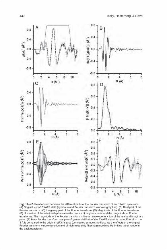
430 Kelly, Hesterberg, & Ravel
Fig.14–22. Relationship between the different parts of the Fourier transform of an EXAFS spectrum. (A) Original c(k)k2 EXAFS data (symbols) and Fourier transform window (gray line). (B) Real part of the Fourier transform. (C) Imaginary part of the Fourier transform. (D) Magnitude of the Fourier transform. (E) Illustration of the relationship between the real and imaginary parts and the magnitude of Fourier transforms. The magnitude of the Fourier transform is like an envelope function of the real and imaginary parts. (F) Back Fourier transform real part of c(q) (solid line) of the EXAFS signal in panel E for R = 1 to 3 Å is compared to the original c(k)k2 signal (connected symbols) to illustrate the effects of the original Fourier transform window function and of high frequency filtering (smoothing by limiting the R range in the back transform).
Mineralogical Methods.indb 430 2/15/2008 2:37:35 PM
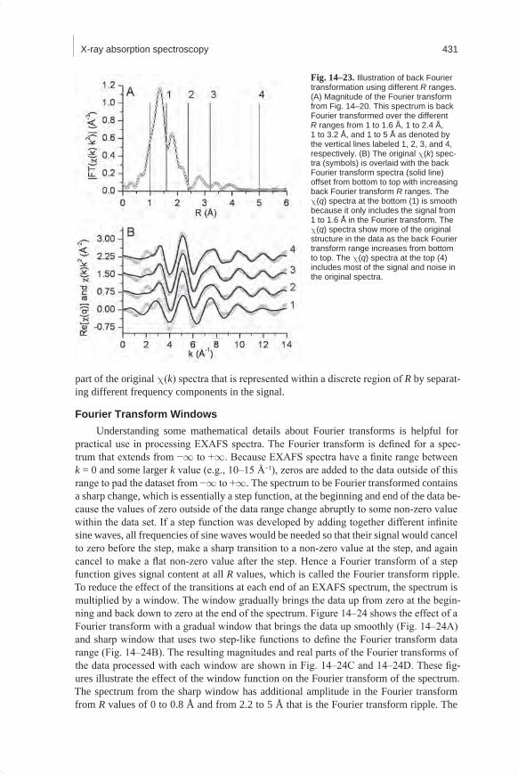
X-ray absorption spectroscopy 431
part of the original c(k) spectra that is represented within a discrete region of R by separat-ing different frequency components in the signal.
Fourier Transform WindowsUnderstanding some mathematical details about Fourier transforms is helpful for
practical use in processing EXAFS spectra. The Fourier transform is defined for a spec-trum that extends from −¥ to +¥. Because EXAFS spectra have a finite range between k = 0 and some larger k value (e.g., 10–15 Å−1), zeros are added to the data outside of this range to pad the dataset from −¥ to +¥. The spectrum to be Fourier transformed contains a sharp change, which is essentially a step function, at the beginning and end of the data be-cause the values of zero outside of the data range change abruptly to some non-zero value within the data set. If a step function was developed by adding together different infinite sine waves, all frequencies of sine waves would be needed so that their signal would cancel to zero before the step, make a sharp transition to a non-zero value at the step, and again cancel to make a flat non-zero value after the step. Hence a Fourier transform of a step function gives signal content at all R values, which is called the Fourier transform ripple. To reduce the effect of the transitions at each end of an EXAFS spectrum, the spectrum is multiplied by a window. The window gradually brings the data up from zero at the begin-ning and back down to zero at the end of the spectrum. Figure 14–24 shows the effect of a Fourier transform with a gradual window that brings the data up smoothly (Fig. 14–24A) and sharp window that uses two step-like functions to define the Fourier transform data range (Fig. 14–24B). The resulting magnitudes and real parts of the Fourier transforms of the data processed with each window are shown in Fig. 14–24C and 14–24D. These fig-ures illustrate the effect of the window function on the Fourier transform of the spectrum. The spectrum from the sharp window has additional amplitude in the Fourier transform from R values of 0 to 0.8 Å and from 2.2 to 5 Å that is the Fourier transform ripple. The
Fig.14–23. Illustration of back Fourier transformation using different R ranges. (A) Magnitude of the Fourier transform from Fig. 14–20. This spectrum is back Fourier transformed over the different R ranges from 1 to 1.6 Å, 1 to 2.4 Å, 1 to 3.2 Å, and 1 to 5 Å as denoted by the vertical lines labeled 1, 2, 3, and 4, respectively. (B) The original c(k) spec-tra (symbols) is overlaid with the back Fourier transform spectra (solid line) offset from bottom to top with increasing back Fourier transform R ranges. The c(q) spectra at the bottom (1) is smooth because it only includes the signal from 1 to 1.6 Å in the Fourier transform. The c(q) spectra show more of the original structure in the data as the back Fourier transform range increases from bottom to top. The c(q) spectra at the top (4) includes most of the signal and noise in the original spectra.
Mineralogical Methods.indb 431 2/15/2008 2:37:36 PM
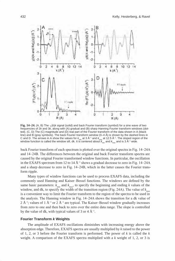
432 Kelly, Hesterberg, & Ravel
back Fourier transform of each spectrum is plotted over the original spectra in Fig. 14–24A and 14–24B. The differences between the original and back Fourier transform spectra are caused by the original Fourier transformed window functions. In particular, the oscillation in the EXAFS spectrum from 12 to 14 Å−1 shows a gradual decrease to zero in Fig. 14–24A and a sharp decrease to zero in Fig. 14–24B, which in the latter causes the Fourier trans-form ripple.
Many types of window functions can be used to process EXAFS data, including the commonly used Hanning and Kaiser–Bessel functions. The windows are defined by the same basic parameters: kmin and kmax, to specify the beginning and ending k values of the window, and dk, to specify the width of the transition region (Fig. 24A). The value of kmax is a convenient way to limit the Fourier transform to the region of the spectra to be used in the analysis. The Hanning window in Fig. 14–24A shows the transition for a dk value of 2 Å−1; values of 1 Å−1 or 2 Å−1 are typical. The Kaiser–Bessel window gradually increases from zero to one and then back to zero over the entire data range. The slope is controlled by the value of dk, with typical values of 3 or 4 Å−1.
Fourier Transform k WeightsThe amplitude of EXAFS oscillations diminishes with increasing energy above the
absorption edge. Therefore, EXAFS spectra are usually multiplied by k raised to the power of 1, 2, or 3 before the Fourier transform is performed. The power of k is called the k weight. A comparison of the EXAFS spectra multiplied with a k weight of 1, 2, or 3 is
Fig.14–24. (A, B) The c(k)k signal (solid) and back Fourier transform (symbol) for a sine wave of two frequencies of 2k and 3k, along with (A) gradual and (B) sharp Hanning Fourier transform windows (dot-ted). (C, D) The (C) magnitude and (D) real part of the Fourier transform of the data shown in A (black line) and B (gray symbols). The back Fourier transform window (0–4 Å) is shown by the dashed lines in C and D. The arrows in A show the values for kmin at 3 Å−1 and kmax at 12.5 Å−1. The sloped region of the window function is called the window sill, dk. It is centered about kmin and kmax and is 3 Å−1 wide.
Mineralogical Methods.indb 432 2/15/2008 2:37:37 PM
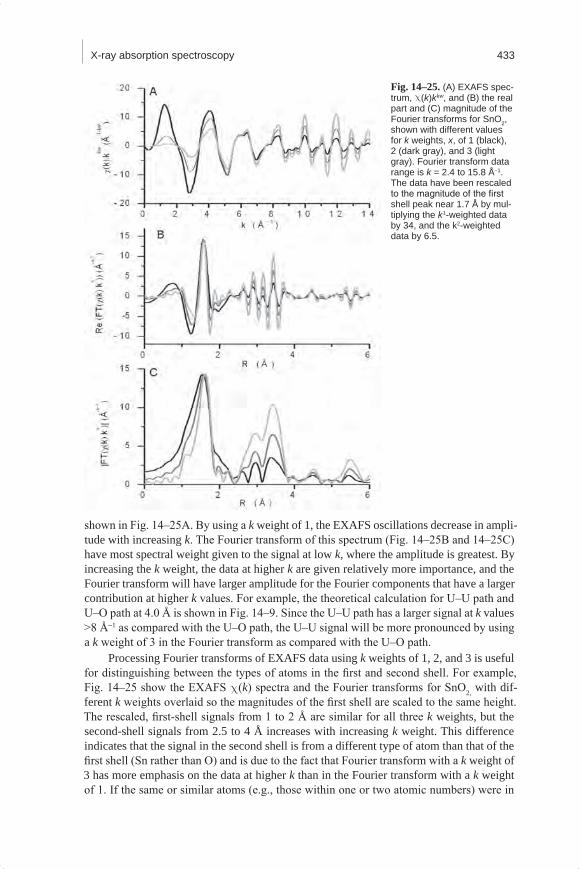
X-ray absorption spectroscopy 433
shown in Fig. 14–25A. By using a k weight of 1, the EXAFS oscillations decrease in ampli-tude with increasing k. The Fourier transform of this spectrum (Fig. 14–25B and 14–25C) have most spectral weight given to the signal at low k, where the amplitude is greatest. By increasing the k weight, the data at higher k are given relatively more importance, and the Fourier transform will have larger amplitude for the Fourier components that have a larger contribution at higher k values. For example, the theoretical calculation for U–U path and U–O path at 4.0 Å is shown in Fig. 14–9. Since the U–U path has a larger signal at k values >8 Å−1 as compared with the U–O path, the U–U signal will be more pronounced by using a k weight of 3 in the Fourier transform as compared with the U–O path.
Processing Fourier transforms of EXAFS data using k weights of 1, 2, and 3 is useful for distinguishing between the types of atoms in the first and second shell. For example, Fig. 14–25 show the EXAFS c(k) spectra and the Fourier transforms for SnO2, with dif-ferent k weights overlaid so the magnitudes of the first shell are scaled to the same height. The rescaled, first-shell signals from 1 to 2 Å are similar for all three k weights, but the second-shell signals from 2.5 to 4 Å increases with increasing k weight. This difference indicates that the signal in the second shell is from a different type of atom than that of the first shell (Sn rather than O) and is due to the fact that Fourier transform with a k weight of 3 has more emphasis on the data at higher k than in the Fourier transform with a k weight of 1. If the same or similar atoms (e.g., those within one or two atomic numbers) were in
Fig.14–25.(A) EXAFS spec-trum, c(k)kkw, and (B) the real part and (C) magnitude of the Fourier transforms for SnO2, shown with different values for k weights, x, of 1 (black), 2 (dark gray), and 3 (light gray). Fourier transform data range is k = 2.4 to 15.8 Å−1. The data have been rescaled to the magnitude of the first shell peak near 1.7 Å by mul-tiplying the k1-weighted data by 34, and the k2-weighted data by 6.5.
Mineralogical Methods.indb 433 2/15/2008 2:37:38 PM
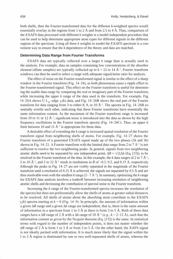
434 Kelly, Hesterberg, & Ravel
both shells, then the Fourier-transformed data for the different k-weighted spectra would essentially overlay in the regions from 1 to 2 Å and from 2.5 to 4 Å. Thus, comparison of the EXAFS data processed with different k weights is a model-independent procedure that can be used to help determine appropriate atom types for different signals in the different regions of the spectrum. Using all three k weights to model the EXAFS spectrum is a con-venient way to ensure that the k dependence of the theory and data are matched.
Determining Data Range from Fourier TransformsEXAFS data are typically collected over a larger k range than is actually used in
the analysis. For example, data on samples containing low concentrations of the absorber element (dilute samples) are typically collected up to k = 12 to 14 Å−1. Fourier transform windows can then be used to select a range with adequate signal/noise ratio for analysis.
The effect of noise on the Fourier-transformed signal is similar to the effect of a sharp window in the Fourier transform (Fig. 14–24), as both phenomena cause a ripple effect in the Fourier-transformed signal. This effect on the Fourier transform is useful for determin-ing the usable data range by comparing the real or imaginary part of the Fourier transform, while increasing the upper k range of the data used in the transform. For example, Fig. 14–26A shows U LIII–edge c(k) data, and Fig. 14–26B shows the real part of the Fourier transform for data ranging from 3 to either 8, 9, or 10 Å−1. The spectra in Fig. 14–26B es-sentially overlie each other, indicating that these Fourier transforms have essentially the same information content. As the maximum of the Fourier transform range is increased from 10 to 11 or 12 Å−1, significant noise is introduced into the data as shown by the high frequency oscillations in the Fourier transform spectra (Fig. 14–26C). Thus, an upper k limit between 10 and 11 Å−1 is appropriate for these data.
A desirable effect of extending the k range is increased spatial resolution of the Fourier transform signal from neighboring shells of atoms. For example, Fig. 14–27 shows the Fourier transform of a generated EXAFS signal made up of the two phases (2k and 3k) shown in Fig. 14–21. A Fourier transform with the limited data range from 2 to 7 Å−1 is not sufficient to resolve the two neighboring peaks. In general, signals from two neighboring atomic shells need to be separated by one independent point, ∆R = p/2Dk (Eq. [15]), to be resolved in the Fourier transform of the data. In this example, the k data ranges of 2 to 7 Å−1, 2 to 10 Å−1, and 2 to 12 Å−1 result in resolutions in R of ~0.3, 0.2, and 0.15 Å, respectively. Although the peaks in Fig. 14–27 are not visibly separated in the magnitude of the Fourier transform until a resolution of 0.15 Å is achieved, the signals are separated by 0.5 Å and are thus resolvable even with the smallest k range (2– 7 Å−1). In summary, optimizing the k range for EXAFS data analysis involves a tradeoff between increasing resolution of neighboring atomic shells and decreasing the contribution of spectral noise to the Fourier transform.
Increasing the k range of the Fourier-transformed spectra increases the resolution of the spectra but does not preferentially allow the shells of atoms at greater radial distances to be resolved. All shells of atoms about the absorbing atom contribute to the EXAFS c(k) spectra starting at k = 0 (Fig. 14–9). In principle, the amount of information within a given ∆R range and a given ∆k range are independent; that is, there is the same amount of information in a spectrum from 1 to 3 Å as there is from 3 to 5 Å. Both of these data ranges have a ∆R range of 2 Å with a ∆k range of 10 Å−1 (e.g., k = 2–12 Å), such that the information content as given by the Nyquist theorem (Eq. [15]) is the same. In statistical terms with regard to the number of independent points, it does not matter whether the ∆R range of 2 Å is from 1 to 3 Å or from 3 to 5 Å. On the other hand, the XAFS signal is not ideally packed with information. It is much more likely that the signal within the 1 to 3 Å region is dominated by one or two well-separated shells of atoms, whereas the
Mineralogical Methods.indb 434 2/15/2008 2:37:38 PM
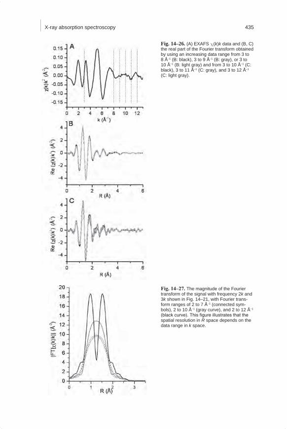
X-ray absorption spectroscopy 435
Fig. 14–27. The magnitude of the Fourier transform of the signal with frequency 2k and 3k shown in Fig. 14–21, with Fourier trans-form ranges of 2 to 7 Å−1 (connected sym-bols), 2 to 10 Å−1 (gray curve), and 2 to 12 Å−1 (black curve). This figure illustrates that the spatial resolution in R space depends on the data range in k space.
Fig.14–26.(A) EXAFS c(k)k data and (B, C) the real part of the Fourier transform obtained by using an increasing data range from 3 to 8 Å−1 (B: black), 3 to 9 Å−1 (B: gray), or 3 to 10 Å−1 (B: light gray) and from 3 to 10 Å−1 (C: black), 3 to 11 Å−1 (C: gray), and 3 to 12 Å−1 (C: light gray).
Mineralogical Methods.indb 435 2/15/2008 2:37:39 PM
436 Kelly, Hesterberg, & Ravel
region from 5 to 7 Å may contain either no signal (e.g., for a hydrated species), a signal from a mixture of many shells of atoms (e.g., for an adsorbed species), or a signal from well-described shells of atoms (e.g., for a metal or oxide mineral).
Random Noise In EXAFS SpectraIn general, the amplitude of the EXAFS part of an X-ray absorption signal is at best
10% of the total absorption signal. In the example shown in Fig. 14–28A, the edge step is approximately 0.3 (from 0.05 to 0.35), and the largest oscillatory part of the absorption coefficient is approximately 0.02 (8% of the edge step). Ideally, the EXAFS signal is 1000 times greater than the random statistical noise (SN). Hence a noise level ≤0.1% of the total signal is desirable. Therefore, if the signal noise is dominated by shot noise, the number of X-rays that need to be measured (NX-ray) is 106 according to the relationship:
X-ray
1SNN
=
[16]
The number of X-rays can be calculated from the voltage on the ionization detectors through Eq. [11]. The noise in EXAFS spectra can be easily approximated by looking at the EXAFS c(k)k2 signal at k = 10 Å−1. At 10 Å−1, the EXAFS signal is usually weak enough that random fluctuations in the data are visible, and by multiplying the data by a factor of 100 via the k2 weighing, y axis values can be considered as percentages. Figure
Fig. 14–28. Illustration of noise in c(k) EXAFS spectrum. (A) X-ray absorption spectrum. (B) Full c(k)k2 EXAFS spectrum. (C) Enlarged view of the c(k)k2 data between 8 and 12 Å−1. The peak to peak noise and the root-mean-square (RMS) noise is shown at 10 Å−1. The fluctuations at 10 Å−1 can be read in percentage because the spectrum is multiplied by 100 during the k weighting of k2 at 10 Å−1.
Mineralogical Methods.indb 436 2/15/2008 2:37:40 PM
X-ray absorption spectroscopy 437
14–28 shows EXAFS data with peak to peak fluctuations at 10 Å−1 of about 0.45%. The root mean square noise is the peak to peak fluctuations divided by 2√2, which is 0.16%, indicating that this data set contains about twice the acceptable noise level. To reduce this noise level by a factor of 2, the statistics need to be increased by a factor of 4 (Eq. [16]) by either increasing the counting time or the number of scans to be averaged. Analogous to the count rate effect on noise, the noise level decreases with the number of scans (Nscans) by a factor Nscans
−1/2. Thus, averaging four scans decreases noise by a factor of two relative to a single scan, assuming that each scan has the same counting time and photon flux. Another source of noise in an EXAFS scan is due to systematic noise caused by sample inhomoge-neity. If the noise in the sample does not decrease with additional counting as given in Eq. [16], then sample preparation should be considered a likely source of noise.
Background FunctionThe EXAFS signal is defined as the normalized oscillatory part of the absorption coef-
ficient above an absorption edge. To process the EXAFS signal, the step-like background of the absorption edge itself is removed. The background function is constructed from splines that are connected with knots. A spline is a polynomial of nth order, where order of 1, 2, or 3 correspond to a linear (y = Ax), quadratic (y = Ax + Bx2), or cubic (y = Ax + Bx2 + Cx3) splines. Early background removal procedures manually placed the knots through the EXAFS oscillations (Sayers and Bunker, 1988). A common more recent approach, called AUTOBK, was developed by Newville et al. (1993) and is integrated into the IFEFFIT methods used by ATHENA. This method uses the information content in the low R region of the spectrum to construct the background function. Information theory is used to define the transfer of information from wavenumber (k) to radial distance (R) through a Fourier transform (Eq. [15]). In this approach, the background function is constructed from third-order (cubic) splines. The knots of the spline are not constrained in the optimization of the background function, which gives less importance to the placement of the knots. The number of splines determines the maximum frequency component that is allowed in the background function. This forces the knots to be evenly spaced in photoelectron wave-number throughout the data region. Information theory is used to constrain the background function to Fourier components that are longer in wavelength than that in the EXAFS spectrum by setting a maximum frequency component in R (called “Rbkg”), below which contributing Fourier components are considered to be part of the background. Because EXAFS oscillations of longer wavelength correspond to shorter radial distances, and vice versa, the longest wavelength oscillation that is actually part of the structural information arises from the first shell of atoms about the absorber.
In the AUTOBK algorithm, the data range and the value for Rbkg determine the number of splines as given by (2RbkgDk)/p. In general, Rbkg is about one-half the first nearest neigh-bor distance. This value for Rbkg will allow all frequencies up to one-half the first shell distance to be removed by the background. The effectiveness of the background removal is made by com-paring the Fourier transform of the c(k) data produced with different values of Rbkg.
Figure 14–29 shows some U LIII–edge data with three very different choices for the value of Rbkg. In the case of Rbkg = 0.5 Å, the background function does not have the flex-ibility to remove the long frequency in the background. The Fourier transform of this c(k) spectrum shows a large peak at 0.5 Å that must be due to the background and not to neighboring atoms in the sample, because interatomic distances between atoms are >1.0 Å, based on ionic radii of anions being >1.2 Å (Lide, 2003). Optimal background removal (Rbkg ~1.0 Å in Fig. 14–29) maximizes the intensity of the first-shell peak while minimizing the amplitudes of peaks at shorter radial distances in the Fourier transform. To the contrary,
Mineralogical Methods.indb 437 2/15/2008 2:37:40 PM
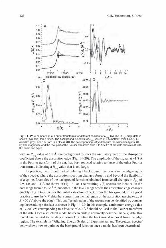
438 Kelly, Hesterberg, & Ravel
with an Rbkg value of 1.5 Å, the background follows the oscillatory part of the absorption coefficient above the absorption edge (Fig. 14–29). The amplitude of the signal at ~1.8 Å in the Fourier transform of the data has been reduced relative to those of the other Fourier transforms, indicating a Rbkg value that is too large.
In practice, the difficult part of defining a background function is in the edge-region of the spectra, where the absorption spectrum changes abruptly and beyond the flexibility of a spline. Examples of the background functions obtained from small changes in Rbkg of 0.9, 1.0, and 1.1 Å are shown in Fig. 14–30. The resulting c(k) spectra are identical in the data range from 3 to 12 Å−1, but differ in the low k range where the absorption edge changes quickly (Fig. 14–30B). For the initial extraction of c(k) from the background, it is a good practice to use the c(k) data that comes from the flat region of the absorption spectra (e.g., at E > 20 eV above the edge). This unaffected region of the spectra can be identified by compar-ing the resulting c(k) data as shown in Fig. 14–30. In this example, a minimum energy value of 17,209 eV corresponding to a k value of 3.0 Å−1 should be used in the Fourier transform of the data. Once a structural model has been built to accurately describe this c(k) data, this model can be used to test data at lower k or refine the background removal from the edge region. The example in “Aligning Energy Scales of Experimental and Theoretical Spectra” below shows how to optimize the background function once a model has been determined.
Fig. 14–29. A comparison of Fourier transforms for different choices for Rbkg. (A) The U LIII–edge data is shown (symbols) three times. The background is shown for Rbkg values of 0.5 (bottom: thick black), 1.0 (middle: gray), and 1.5 (top: thin black). (B) The corresponding c(k)k data with the same line types. (C, D) The magnitude and the real part of the Fourier transform from 3 to 9.5 Å−1 of the data shown in B with the same line types.
Mineralogical Methods.indb 438 2/15/2008 2:37:41 PM
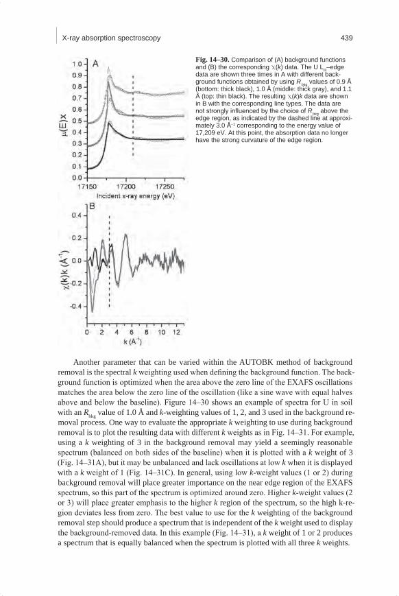
X-ray absorption spectroscopy 439
Another parameter that can be varied within the AUTOBK method of background removal is the spectral k weighting used when defining the background function. The back-ground function is optimized when the area above the zero line of the EXAFS oscillations matches the area below the zero line of the oscillation (like a sine wave with equal halves above and below the baseline). Figure 14–30 shows an example of spectra for U in soil with an Rbkg value of 1.0 Å and k-weighting values of 1, 2, and 3 used in the background re-moval process. One way to evaluate the appropriate k weighting to use during background removal is to plot the resulting data with different k weights as in Fig. 14–31. For example, using a k weighting of 3 in the background removal may yield a seemingly reasonable spectrum (balanced on both sides of the baseline) when it is plotted with a k weight of 3 (Fig. 14–31A), but it may be unbalanced and lack oscillations at low k when it is displayed with a k weight of 1 (Fig. 14–31C). In general, using low k-weight values (1 or 2) during background removal will place greater importance on the near edge region of the EXAFS spectrum, so this part of the spectrum is optimized around zero. Higher k-weight values (2 or 3) will place greater emphasis to the higher k region of the spectrum, so the high k-re-gion deviates less from zero. The best value to use for the k weighting of the background removal step should produce a spectrum that is independent of the k weight used to display the background-removed data. In this example (Fig. 14–31), a k weight of 1 or 2 produces a spectrum that is equally balanced when the spectrum is plotted with all three k weights.
Fig.14–30.Comparison of (A) background functions and (B) the corresponding c(k) data. The U LIII–edge data are shown three times in A with different back-ground functions obtained by using Rbkg values of 0.9 Å (bottom: thick black), 1.0 Å (middle: thick gray), and 1.1 Å (top: thin black). The resulting c(k)k data are shown in B with the corresponding line types. The data are not strongly influenced by the choice of Rbkg above the edge region, as indicated by the dashed line at approxi-mately 3.0 Å−1 corresponding to the energy value of 17,209 eV. At this point, the absorption data no longer have the strong curvature of the edge region.
Mineralogical Methods.indb 439 2/15/2008 2:37:41 PM
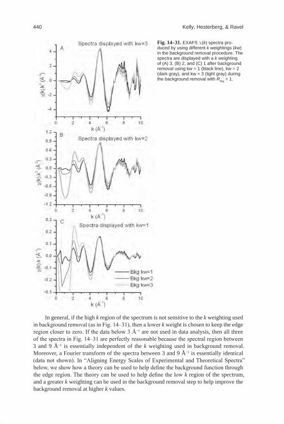
440 Kelly, Hesterberg, & Ravel
In general, if the high k region of the spectrum is not sensitive to the k weighting used in background removal (as in Fig. 14–31), then a lower k weight is chosen to keep the edge region closer to zero. If the data below 3 Å−1 are not used in data analysis, then all three of the spectra in Fig. 14–31 are perfectly reasonable because the spectral region between 3 and 9 Å−1 is essentially independent of the k weighting used in background removal. Moreover, a Fourier transform of the spectra between 3 and 9 Å−1 is essentially identical (data not shown). In “Aligning Energy Scales of Experimental and Theoretical Spectra” below, we show how a theory can be used to help define the background function through the edge region. The theory can be used to help define the low k region of the spectrum, and a greater k weighting can be used in the background removal step to help improve the background removal at higher k values.
Fig.14–31.EXAFS c(k) spectra pro-duced by using different k weightings (kw) in the background removal procedure. The spectra are displayed with a k weighting of (A) 3, (B) 2, and (C) 1 after background removal using kw = 1 (black line), kw = 2 (dark gray), and kw = 3 (light gray) during the background removal with Rbkg = 1.
Mineralogical Methods.indb 440 2/15/2008 2:37:42 PM
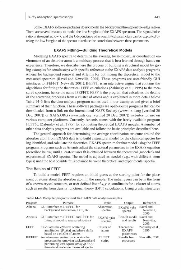
X-ray absorption spectroscopy 441
Some EXAFS software packages do not model the background throughout the edge region. There are several reasons to model the low k region of the EXAFS spectrum. The signal/noise ratio is strongest at low k, and the k dependence of several fitted parameters can be exploited by using the low k region of the spectra to reduce the correlation between these parameters.
EXAFS Fitting—Building Theoretical ModelsModeling EXAFS spectra to determine the average, local-molecular coordination en-
vironment of an absorber atom is a multistep process that is best learned through hands-on experience. Therefore, we describe here the process of building a structural model by giv-ing examples for certain steps with specific reference to the EXAFS data analysis programs Athena for background removal and Artemis for optimizing the theoretical model to the measured spectrum (Ravel and Newville, 2005). These programs are user-friendly GUI interfaces to IFEFFIT (Newville 2001). IFEFFIT is an interactive engine that contains the algorithms for fitting the theoretical FEFF calculations (Zabinsky et al., 1995) to the mea-sured spectrum, hence the name IFEFFIT. FEFF is the program that calculates the details of the scattering processes from a cluster of atoms and is explained in more detail below. Table 14–3 lists the data-analysis program names used in our examples and gives a brief summary of their function. These software packages are open-source programs that can be downloaded from a link on the International XAFS Society (www.i-x-s.org [verified 20 Dec. 2007]) or XAFS.ORG (www.xafs.org [verified 20 Dec. 2007]) websites for use on various computer platforms. Currently, Artemis comes with the freely available program FEFF6L (Zabinsky et al., 1995) for computing theoretical EXAFS models. A number of other data analysis programs are available and follow the basic principles described here.
The general approach for determining the average coordination structure around the absorber atom from EXAFS data is to build a structural model for the chemical species be-ing identified, and calculate the theoretical EXAFS spectrum for that model using the FEFF program. Programs such as Artemis adjust the structural parameters in the EXAFS equation (described below) until a least-squares fit is obtained between the theoretical (modeled) and experimental EXAFS spectra. The model is adjusted as needed (e.g., with different atom types) until the best possible fit is obtained between theoretical and experimental spectra.
The Basics of FEFFTo build a model, FEFF requires an initial guess as the starting point for the place-
ment of atoms about the absorber atom in the sample. The initial guess can be in the form of a known crystal structure, or user-defined list of x, y, z coordinates for a cluster of atoms, such as results from density functional theory (DFT) calculations. Using crystal structures
Table14–3.Computer programs used the EXAFS data analysis examples.
Program Purpose Input Output ReferenceAthena GUI interface to IFEFFIT for
background subtraction, LCF, etc.Absorption
spectraEXAFS c(k)
spectraRavel and
Newville, 2005
Artemis GUI interface to IFEFFIT and FEFF for fitting a model to measured spectra
EXAFS c(k) spectra
Best-fit model and results
Ravel and Newville, 2005
FEFF Calculates the effective scattering amplitudes [(Feff(k)] and phase shifts based on a cluster of atoms
Cluster of atoms
Theoretical EXAFS parameters
Zabinsky et al., 1995
IFEFFIT An interactive engine that contains the processes for removing background and performing least-square fitting of FEFF theoretical models to measured spectra.
IFEFFIT script
Results from processes
Newville, 2001
Mineralogical Methods.indb 441 2/15/2008 2:37:42 PM
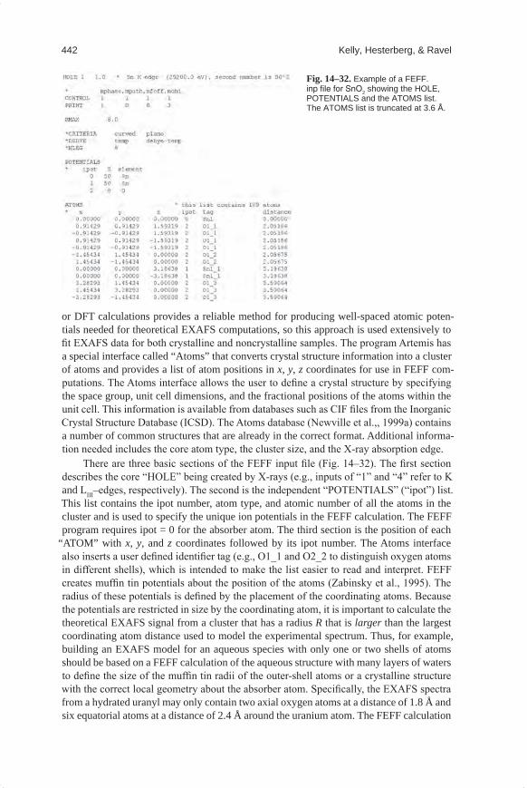
442 Kelly, Hesterberg, & Ravel
or DFT calculations provides a reliable method for producing well-spaced atomic poten-tials needed for theoretical EXAFS computations, so this approach is used extensively to fit EXAFS data for both crystalline and noncrystalline samples. The program Artemis has a special interface called “Atoms” that converts crystal structure information into a cluster of atoms and provides a list of atom positions in x, y, z coordinates for use in FEFF com-putations. The Atoms interface allows the user to define a crystal structure by specifying the space group, unit cell dimensions, and the fractional positions of the atoms within the unit cell. This information is available from databases such as CIF files from the Inorganic Crystal Structure Database (ICSD). The Atoms database (Newville et al.,, 1999a) contains a number of common structures that are already in the correct format. Additional informa-tion needed includes the core atom type, the cluster size, and the X-ray absorption edge.
There are three basic sections of the FEFF input file (Fig. 14–32). The first section describes the core “HOLE” being created by X-rays (e.g., inputs of “1” and “4” refer to K and LIII–edges, respectively). The second is the independent “POTENTIALS” (“ipot”) list. This list contains the ipot number, atom type, and atomic number of all the atoms in the cluster and is used to specify the unique ion potentials in the FEFF calculation. The FEFF program requires ipot = 0 for the absorber atom. The third section is the position of each
“ATOM” with x, y, and z coordinates followed by its ipot number. The Atoms interface also inserts a user defined identifier tag (e.g., O1_1 and O2_2 to distinguish oxygen atoms in different shells), which is intended to make the list easier to read and interpret. FEFF creates muffin tin potentials about the position of the atoms (Zabinsky et al., 1995). The radius of these potentials is defined by the placement of the coordinating atoms. Because the potentials are restricted in size by the coordinating atom, it is important to calculate the theoretical EXAFS signal from a cluster that has a radius R that is larger than the largest coordinating atom distance used to model the experimental spectrum. Thus, for example, building an EXAFS model for an aqueous species with only one or two shells of atoms should be based on a FEFF calculation of the aqueous structure with many layers of waters to define the size of the muffin tin radii of the outer-shell atoms or a crystalline structure with the correct local geometry about the absorber atom. Specifically, the EXAFS spectra from a hydrated uranyl may only contain two axial oxygen atoms at a distance of 1.8 Å and six equatorial atoms at a distance of 2.4 Å around the uranium atom. The FEFF calculation
Fig.14–32.Example of a FEFF.inp file for SnO2 showing the HOLE, POTENTIALS and the ATOMS list. The ATOMS list is truncated at 3.6 Å.
Mineralogical Methods.indb 442 2/15/2008 2:37:42 PM
X-ray absorption spectroscopy 443
based on this cluster will not be accurate because the outer equatorial oxygen atoms do not have well-defined radii since there are no atoms of larger radial distance to define the atom boundaries. The FEFF calculation of a uranyl oxide crystal structure with a cluster size of only 2.4 Å would be similarly incorrect. The FEFF calculation based on the crystal structure of a uranyl oxide to 4 Å including all the atoms beyond the first equatorial oxygen shell will yield improved calculations for the first shell equatorial oxygen atoms to be used to model the hydrated species.
Parameterizing EXAFS VariablesOnce a path has been selected for possible inclusion in a structural model, math-
ematical expressions for the EXAFS parameters (Eq. [5]) are defined. The parameters that are often determined from a fit to the EXAFS spectrum affect either the amplitude of the EXAFS oscillations (N, S0
2, s2) or the phase of the oscillations (∆E0 and ∆R).There are many approaches that can be used to constrain the EXAFS fitting param-
eters such that the number of independent points in the measured spectra is greater than the number of variables determined in the model. Example approaches include collecting EXAFS data at multiple edges and co-refining the fitting parameters (Ravel et al., 1999), using independent structural information and bond angles (Frenkel et al., 1994), modeling a mixture of structures (Kelly et al., 1998), determining binding sites (Kelly et al., 2002), integrating results from multiple techniques (Allen et al., 1995), measuring pressure de-pendence (Frenkel et al., 1997), or temperature dependence (Haskel et al., 2005; Frenkel et al., 2001) of the structures, using multiple edges to obtain structural disorder (Calvin et al., 2002), and using crystal structural information (Ravel et al., 1998). We discuss common approaches for constraining each of the EXAFS fitting parameters:
∆R. First, ∆R values can be defined by an isotropic expansion–contraction term as aReff. Reff is a special key word for the effective path length R for each path from the FEFF calculation of the model structure. A single value of a could be determined and applied to all path lengths included in the model, effectively reducing the number of variables for R from the number of paths (i.e., 30) to a single variable. Because this approach as-sumes that adjustments to all path lengths (interatomic distances) in the structure vary in proportion to one another (a being the proportionality constant), this approach is best used for cubic crystal structures in which physical expansions/contractions are likely to be isotropic. Second, ∆Ri values or aiReff values can be grouped depending on path length or direction. This parameterization gives more freedom to account for an anisotropic expan-sion–contraction but also requires more variables. Third, ∆R values can be related to unit cell dimensions or atomic moieties. This method requires more sophisticated mathemati-cal expressions that are usually derived from known relationships between interatomic distances in specific crystal structures, and it can be very powerful. Some specialized codes have been written to produce these expressions (Kelly et al., 2001). Fourth, the change in path length parameters can be determined independently for each path.
∆E. First, one energy shift can be applied to all paths. This is the most common method of defining ∆E, and it accounts for the misalignment of the data with re-spect to the theoretical calculation. Second, two energy shift values are sometimes used, where the value for the first path is different from the value for all other paths. This method accounts for the energy-alignment issue and for some possible charge imbalance in the FEFF calculation of the first atomic potentials as compared with all other potentials. Third, energy shifts can be assigned to atom types. This method is sometimes used to account for ionic bonds that transfer charge between different types of atoms. In general, these shifts should be less than 2 to 3 eV.
s2. First, s2 values can be defined in terms of a Debye or Einstein model (Sevillano et al., 1979) with one or more characteristic temperatures. Second, s2 values can be grouped depending on atom type and bond length of a model path. This pa-rameterization assumes that coordination shells involving similar atoms and similar
·
·
·
Mineralogical Methods.indb 443 2/15/2008 2:37:42 PM
444 Kelly, Hesterberg, & Ravel
interatomic distances are similar in thermal and static disorder. Third, s2 values can be broken into two components to represent the structural and thermal disorder in the bond lengths. This parameterization can be used with Debye or Einstein models for defining the thermal component, or it can be applied to temperature or pressure dependent spectra. Fourth, a unique s2 value can be given to each path, which yields the maximum number of s2 parameters in the model.
S02. First, one value of S0
2 is often used for all paths included in the model. Second, S0
2 values are determined by fitting the measured EXAFS spectrum of a standard of known crystal structure measured under similar conditions as the sample in which unknown species are being identified. Third, theoretical calculations such as those by FEFF 8.4 (Ankudinov et al., 2003) can also be used to determine S0
2.
N. First, the degeneracy of a path, N, is often determined from the coordination number in a known crystal structure or known atomic species. Second, the degen-eracy can be independently determined for each single scattering path used in the mode. The degeneracy of multiple scattering paths is constrained in terms of the corresponding single scattering paths. Third, coordination numbers can also be con-strained by the stoichiometry of a particular ligand attached to the absorber.
Comparing Models Using Statistical ToolsOnce a model for the EXAFS parameters has been developed, the variable EXAFS
parameters and mathematical variables are adjusted to arrive at a least-squares fit between the experimental and theoretical spectra. The fitting results include the user defined vari-ables, their best-fit values, and the uncertainties in these variables, along with important information about the statistics of the model. Statistical parameters include the number of independent points, Nidp, the number of variables Nvar, which must be less than the number of independent points, the c2 (chi-square) and c2
n (reduced-chi-square) values, and an R factor. These standard goodness-of fit parameters are described in more detail in Bevington and Robinson (1992). Use of these statistical parameters for EXAFS analysis is described by Stern et al. (1995). The isolated EXAFS signal is denoted as c(k) and should not be confused with the goodness-of-fit parameter c2. Changes in the goodness-of-fit parameter, c2
n, are used to compare different EXAFS models.The R factor is the sum of the squares of the differences between the data and the fit at
each data point, divided by the sum of the squares of the data at each corresponding point. It represents the mean square misfit between the data and the fit for both the real and imagi-nary parts of the Fourier transform and is defined as follows:
( )2data fit factor
data
i ii
2i
i
R =-å
å [17]
In general, R factor values less than 0.05 are considered to reflect a reasonable fit.The c2 value is the sum of the squares of the difference between the predicted fit and
the data divided by the uncertainties (e) at each data point (i). It is calculated as
2idp2
pts
data fiti i
ii
N=
N
æ ö- ÷ç ÷çc ÷ç ÷÷ç eè øå [18]
where the sum is over each data point in the real and imaginary parts of the Fourier trans-form, Nidp is the number of independent points in the model fit (Eq. [15]), and Npts is the number of data points. To compare models with different numbers of variables, the c2
n values are used. It is calculated by the c2 divided by the degrees of freedom in the fit, n.
·
·
Mineralogical Methods.indb 444 2/15/2008 2:37:43 PM
X-ray absorption spectroscopy 445
The degrees-of-freedom in the fit is defined as the number of independent points in the measured spectra minus the number of variables fit in the model.
For a general implementation, the c2n value is approximately one for an optimized
model. This guideline is true for systems with well-defined line shapes and uncertainties that can be quantitatively measured such as statistical noise. It may be possible to quantita-tively define nonstatistical errors, but unless they are Gaussian distributed, formal Gaussian statistics will not apply. For XANES and EXAFS analysis, neither the line shapes nor the uncertainties are well defined, resulting in a poorly scaled c2
n value. The uncertainties (e) in EXAFS analysis is based on the amplitude of the EXAFS signal at 15 to 25 Å because there is rarely any contribution from atoms at these distances (Newville et al., 1999b).
The size of the uncertainty e is assumed to be underestimated by the value of c2n, and
this uncertainty is propagated to the uncertainty in the fitting parameters. For example, if the c2
n value of a perfectly reasonable fit is 25 instead of 1, then the uncertainties are increased by Öc2
n or 5 to rescale the c2n value to one. This rescaling is automatically
performed for each fit, so that large c2n values result in large uncertainties in the fitted
parameters. This methodology does not assign any error to the unknown line shapes in EXAFS spectra, and leads to a conservative uncertainty in the measured parameters.
A statistically significant change in the final c2nf value when compared with an ini-
tial c2n i value is greater than two standard deviations:
2
221 2i
f
n
n
c- ³
nc [19]
This equation implies that significant changes in the c2n value are on the order of factors of
2. For example, a final smaller c2n of 40 is better than an initial larger c2
n of 80, but models with c2
n of 40 and 42 are not significantly different.
EXAFS Modeling ExamplesSpecific examples are provided here to illustrate typical, useful procedures for build-
ing a structural model and fitting EXAFS data.
Aligning Energy Scales of Experimental and Theoretical SpectraOne of the steps involved in modeling EXAFS data is aligning the EXAFS spectra to
the theoretically calculated spectra. During background removal, the absorption spectrum as a function of energy (E) is transformed into the EXAFS spectrum as a function of wave-number (k) as defined in Eq. [7]. The wavenumber scale is defined relative to E0, which is a user-defined value. The theoretical spectrum is given as a function of wavenumber k, but the energy used for E0 = 0 (and therefore k = 0) as defined from the measured spectrum rarely coincides with that determined in the theoretical model. As noted above, a fitted pa-rameter, DE0 can be adjusted in the fit of the theory to the data to account for the mismatch between the user defined position of E0 on the edge and the theoretically calculated value for k = 0. In general, DE0 should be kept as small as possible (a few electronvolts) because shifting the energy scale for the theoretical calculation distorts the theoretical spectrum. Very large values for DE0 (tens of electronvolts) can shift the spectra by a full oscillation in the EXAFS spectrum and lead to erroneous inter-atomic distances (Michalowicz and Vlaic, 1998). By aligning the experimental and theoretical spectra, the theoretical edge energy, E0, is defined relative to measured data. This procedure ensures that the E0 value falls on the edge of the absorption coefficient, thereby preventing a mismatch between
Mineralogical Methods.indb 445 2/15/2008 2:37:43 PM
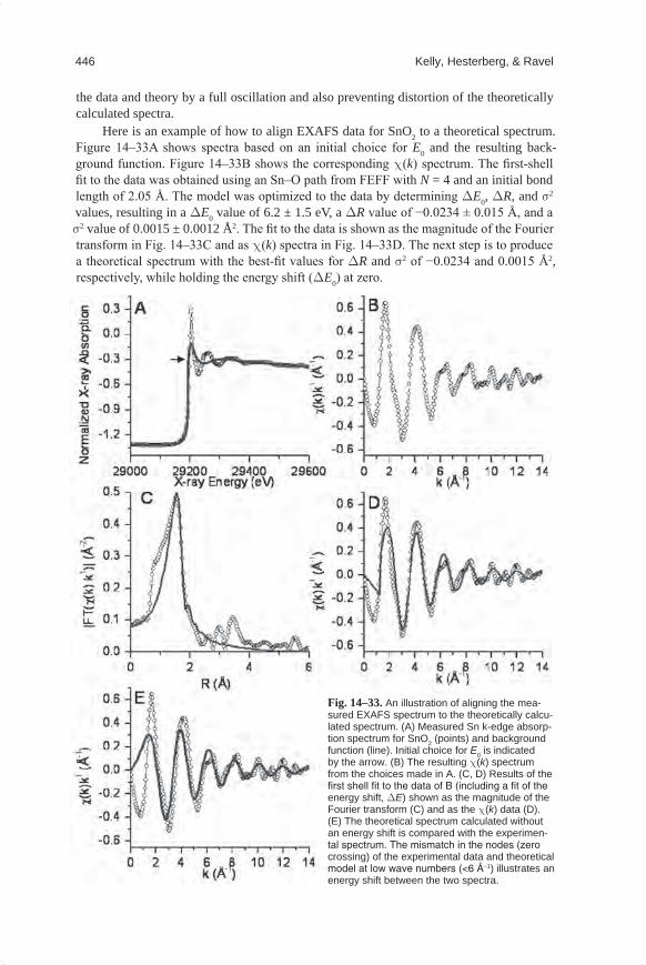
446 Kelly, Hesterberg, & Ravel
the data and theory by a full oscillation and also preventing distortion of the theoretically calculated spectra.
Here is an example of how to align EXAFS data for SnO2 to a theoretical spectrum. Figure 14–33A shows spectra based on an initial choice for E0 and the resulting back-ground function. Figure 14–33B shows the corresponding c(k) spectrum. The first-shell fit to the data was obtained using an Sn–O path from FEFF with N = 4 and an initial bond length of 2.05 Å. The model was optimized to the data by determining DE0, DR, and s2 values, resulting in a DE0 value of 6.2 ± 1.5 eV, a DR value of −0.0234 ± 0.015 Å, and a s2 value of 0.0015 ± 0.0012 Å2. The fit to the data is shown as the magnitude of the Fourier transform in Fig. 14–33C and as c(k) spectra in Fig. 14–33D. The next step is to produce a theoretical spectrum with the best-fit values for DR and s2 of −0.0234 and 0.0015 Å2, respectively, while holding the energy shift (DE0) at zero.
Fig.14–33.An illustration of aligning the mea-sured EXAFS spectrum to the theoretically calcu-lated spectrum. (A) Measured Sn k-edge absorp-tion spectrum for SnO2 (points) and background function (line). Initial choice for E0 is indicated by the arrow. (B) The resulting c(k) spectrum from the choices made in A. (C, D) Results of the first shell fit to the data of B (including a fit of the energy shift, DE) shown as the magnitude of the Fourier transform (C) and as the c(k) data (D). (E) The theoretical spectrum calculated without an energy shift is compared with the experimen-tal spectrum. The mismatch in the nodes (zero crossing) of the experimental data and theoretical model at low wave numbers (<6 Å−1) illustrates an energy shift between the two spectra.
Mineralogical Methods.indb 446 2/15/2008 2:37:44 PM
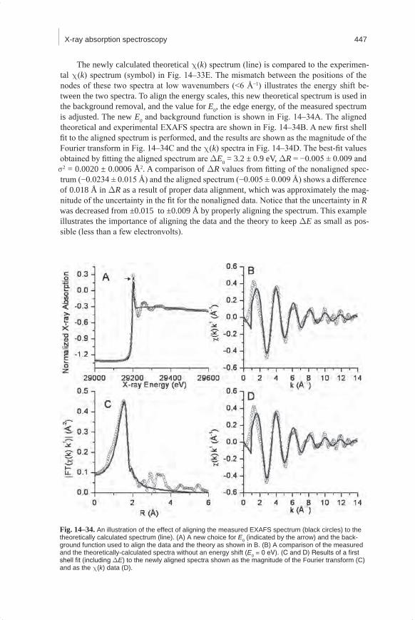
X-ray absorption spectroscopy 447
The newly calculated theoretical c(k) spectrum (line) is compared to the experimen-tal c(k) spectrum (symbol) in Fig. 14–33E. The mismatch between the positions of the nodes of these two spectra at low wavenumbers (<6 Å−1) illustrates the energy shift be-tween the two spectra. To align the energy scales, this new theoretical spectrum is used in the background removal, and the value for E0, the edge energy, of the measured spectrum is adjusted. The new E0 and background function is shown in Fig. 14–34A. The aligned theoretical and experimental EXAFS spectra are shown in Fig. 14–34B. A new first shell fit to the aligned spectrum is performed, and the results are shown as the magnitude of the Fourier transform in Fig. 14–34C and the c(k) spectra in Fig. 14–34D. The best-fit values obtained by fitting the aligned spectrum are DE0 = 3.2 ± 0.9 eV, DR = −0.005 ± 0.009 and s2 = 0.0020 ± 0.0006 Å2. A comparison of DR values from fitting of the nonaligned spec-trum (−0.0234 ± 0.015 Å) and the aligned spectrum (−0.005 ± 0.009 Å) shows a difference of 0.018 Å in DR as a result of proper data alignment, which was approximately the mag-nitude of the uncertainty in the fit for the nonaligned data. Notice that the uncertainty in R was decreased from ±0.015 to ±0.009 Å by properly aligning the spectrum. This example illustrates the importance of aligning the data and the theory to keep DE as small as pos-sible (less than a few electronvolts).
Fig.14–34.An illustration of the effect of aligning the measured EXAFS spectrum (black circles) to the theoretically calculated spectrum (line). (A) A new choice for E0 (indicated by the arrow) and the back-ground function used to align the data and the theory as shown in B. (B) A comparison of the measured and the theoretically-calculated spectra without an energy shift (E0 = 0 eV). (C and D) Results of a first shell fit (including DE) to the newly aligned spectra shown as the magnitude of the Fourier transform (C) and as the c(k) data (D).
Mineralogical Methods.indb 447 2/15/2008 2:37:44 PM
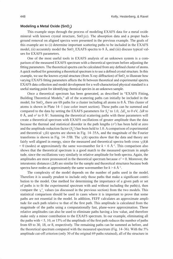
448 Kelly, Hesterberg, & Ravel
Modeling a Metal Oxide (SnO2)This example steps through the process of modeling EXAFS data for a metal oxide
mineral with known crystal structure, SnO2(c). The absorption data and a proper back-ground removal on aligned spectra were presented in the previous example. The goals of this example are to (i) determine important scattering paths to be included in the EXAFS model, (ii) accurately model the SnO2 EXAFS spectra to 8 Å, and (iii) discuss typical val-ues for EXAFS parameters.
One of the most useful tools in EXAFS analysis of an unknown system is a com-parison of the measured EXAFS spectrum with a theoretical spectrum before adjusting the fitting parameters. The theoretical spectra can be calculated from any defined cluster of atoms. A quick method for generating a theoretical spectrum is to use a defined crystal structure. In this example, we use the known crystal structure (from X-ray diffraction) of SnO2 to illustrate how varying EXAFS fitting parameters affects the fit between theoretical and experimental spectra. EXAFS data collection and model development for a well-characterized physical standard is a useful starting point for identifying chemical species in an unknown sample.
Once a theoretical spectrum has been generated, as described in “EXAFS Fitting, Building Theoretical Models,” all of the scattering paths can initially be included in the model; for SnO2, there are 69 paths for a cluster including all atoms to 8 Å. This cluster of atoms is shown in Plate 14–1 (see color insert section). These paths can be summed and compared to the data by setting the EXAFS parameters for S0
2 to 1.0, DE0 to 0 eV, DR to 0 Å, and s2 to 0 Å2. Summing the theoretical scattering paths with these parameters will create a theoretical spectrum with EXAFS oscillations of greater amplitude than the data because the thermal and statistical disorder in the path lengths (s2) has been held at zero and the amplitude reduction factor (S0
2) has been held to 1.0. A comparison of experimental and theoretical c(k) spectra are shown in Fig. 14–35A, and the magnitude of the Fourier transforms is shown in Fig. 14–35B. The c(k) spectra show that the data and theory are fairly well aligned in energy, since the measured and theoretical spectra both cross c(k)k
= 0 (nodes) at approximately the same wavenumber for k < 6 Å−1. This comparison also shows that the theoretical spectrum is a good match to the measured spectrum in ampli-tude, since the oscillations vary similarly in relative amplitude for both spectra. Again, the amplitudes are more pronounced in the theoretical spectrum because s2 = 0. Moreover, the interatomic distances (DR) are similar for the sample and theoretical structures because both spectra have nodes at approximately the same wavenumber for k > 6 Å−1.
The complexity of the model depends on the number of paths used in the model. Therefore it is usually prudent to include only those paths that make a significant contri-bution to the model. One method for determining the importance of a given path or set of paths is to fit the experimental spectrum with and without including the path(s), then compare the c2
n values (as discussed in the previous section) from the two models. This statistical comparison should be used in cases where it is important to prove that some paths are not essential in the model. In addition, FEFF calculates an approximate ampli-tude for each path relative to that of the first path. This amplitude is calculated from the magnitude of the paths using a computationally fast, plane-wave approximation. These relative amplitudes can also be used to eliminate paths having a low value, and therefore make only a minor contribution to the EXAFS spectrum. In our example, eliminating all the paths with < 5, 10, or 15% of the amplitude of the first path reduces the number of paths from 69 to 30, 18, or 8, respectively. The remaining paths can be summed as before, and the theoretical spectrum compared with the measured spectrum (Fig. 14–36). With the 5% amplitude cut-off criterion (only 30 of the original 69 paths retained), all of the structure in
Mineralogical Methods.indb 448 2/15/2008 2:37:45 PM
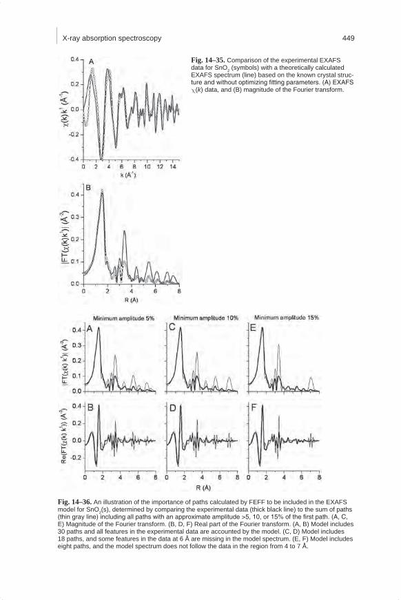
X-ray absorption spectroscopy 449
Fig.14–35. Comparison of the experimental EXAFS data for SnO2 (symbols) with a theoretically calculated EXAFS spectrum (line) based on the known crystal struc-ture and without optimizing fitting parameters. (A) EXAFS c(k) data, and (B) magnitude of the Fourier transform.
Fig.14–36. An illustration of the importance of paths calculated by FEFF to be included in the EXAFS model for SnO2(s), determined by comparing the experimental data (thick black line) to the sum of paths (thin gray line) including all paths with an approximate amplitude >5, 10, or 15% of the first path. (A, C, E) Magnitude of the Fourier transform. (B, D, F) Real part of the Fourier transform. (A, B) Model includes 30 paths and all features in the experimental data are accounted by the model. (C, D) Model includes 18 paths, and some features in the data at 6 Å are missing in the model spectrum. (E, F) Model includes eight paths, and the model spectrum does not follow the data in the region from 4 to 7 Å.
Mineralogical Methods.indb 449 2/15/2008 2:37:45 PM
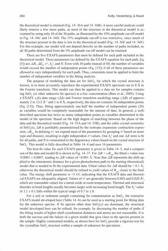
450 Kelly, Hesterberg, & Ravel
the theoretical model is retained (Fig. 14–36A and 14–36B). A more careful analysis could likely remove a few more paths, as most of the structure in the theoretical model is ac-counted by using only 18 of the 30 paths, as illustrated by the 10% amplitude cut-off model in Fig. 14–36C and 14–36D. The 15% amplitude cut-off is too restrictive, since much of the structure present in the data is lost in the theoretical model (Fig. 14–36E and 14–36F). For this example, our model will not depend directly on the number of paths included, so all 30 paths determined from the 5% amplitude cut-off model can be retained.
There are five EXAFS parameters that must be defined for each path included in the theoretical model. These parameters (as defined by the EXAFS equation for each path, Eq. [5]) are DR, DE0, s
2, S02, and N. Even with 30 paths instead of 69, the number of variables
would exceed the number of independent points (Eq. [15]) if all of these parameters are allowed to vary independently for each path. Thus, constraints must be applied to limit the number of independent variables in the fitting analysis.
The purpose of modeling the data set for SnO2, for which the crystal structure is known, is to most accurately reproduce the experimental EXAFS spectrum out to 8 Å in the Fourier transform. This model can then be applied to a data set for samples contain-ing SnO2 (or other unknown Sn species) at a low concentration (Bare et al., 2005). Using a EXAFS c(k) data range (Dk) and Fourier transform modeling range (DR) of approxi-mately 2 to 13.5 Å−1 and 1 to 8 Å, respectively, the data set contains 56 independent points (Eq. [15]). Thus, fitting approximately one-half the number of independent points (28) as variables would be completely reasonable for the amount of data. In general, a well-described spectrum has twice as many independent points as variables determined in the model of the spectrum. Based on the high degree of matching between the phase of the data and the theoretical model (Fig. 14–35A and 14–35B), and the cubic crystal symmetry of SnO2(s), DR is justifiably parameterized by the isotropic expansion–contraction expres-sion, aReff. In defining s2, we expend most of the parameters by grouping s2 based on atom type and distance, resulting in eight independent s2 values. One S0
2 and one DE term is fit for all paths, and N is constrained to the degeneracy values based on the crystal structure of SnO2. This model is fully described in Table 14–4 and uses 16 parameters.
The best-fit value for each EXAFS parameter is given in Table 14–5, and a compari-son of the data and model fit is shown in Fig. 14–37. For DR = aReff, the fitted a value was
−0.0001 ± 0.0007, leading to DR values of <0.001 Å. Note that DR represents the shift ap-plied to the interatomic distance for a given photoelectron path in the starting (theoretical) model that is needed to fit the experimental data. Fitted values for DR should be < 0.1 Å; otherwise the theoretical model should be refined to yield values of Rreff closer to the final value. The energy shift parameter is <5 eV, indicating that the EXAFS data and theoreti-cal EXAFS are adequately aligned. Values of s2 are generally between 0.003 and 0.020 Å2, which are reasonable values for a metal oxide at room temperature. Thermal and structural disorder in bond lengths usually becomes larger with increasing bond length. The S0
2 value of 1.1 ± 0.1 falls within the typical range of 0.7 to 1.0.
For a soil or sediment sample containing Sn contamination as SnO2, the extensive EXAFS model developed here (Table 14–4) can be used as a starting point for fitting data for the unknown species. If Sn species other than SnO2(c) are dominant, the structural model developed here can be refined, for example, by decreasing the number of paths if the fitting results of higher-shell coordination distances and atoms are not reasonable. It is both the success and the failure of a given model that give clues to the species present in the sample. Highly constrained models, as shown here for SnO2 provide a rigorous test for the crystalline SnO2 structure within a sample of unknown Sn speciation.
Mineralogical Methods.indb 450 2/15/2008 2:37:46 PM
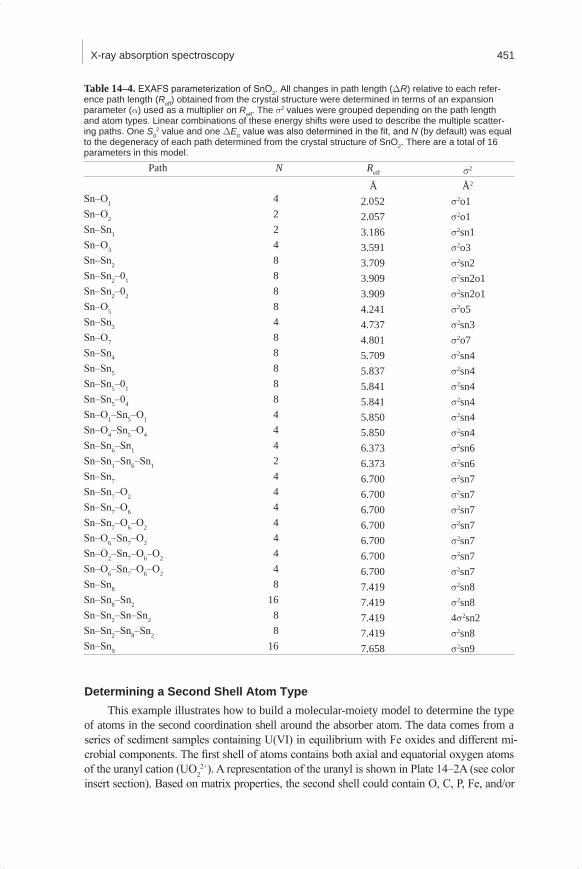
X-ray absorption spectroscopy 451
Determining a Second Shell Atom TypeThis example illustrates how to build a molecular-moiety model to determine the type
of atoms in the second coordination shell around the absorber atom. The data comes from a series of sediment samples containing U(VI) in equilibrium with Fe oxides and different mi-crobial components. The first shell of atoms contains both axial and equatorial oxygen atoms of the uranyl cation (UO2
2+). A representation of the uranyl is shown in Plate 14–2A (see color insert section). Based on matrix properties, the second shell could contain O, C, P, Fe, and/or
Table14–4.EXAFS parameterization of SnO2. All changes in path length (DR) relative to each refer-ence path length (Reff) obtained from the crystal structure were determined in terms of an expansion parameter (a) used as a multiplier on Reff. The s2 values were grouped depending on the path length and atom types. Linear combinations of these energy shifts were used to describe the multiple scatter-ing paths. One S0
2 value and one DE0 value was also determined in the fit, and N (by default) was equal to the degeneracy of each path determined from the crystal structure of SnO2. There are a total of 16 parameters in this model.
Path N Reff s2
Å Å2
Sn–O1 4 2.052 s2o1Sn–O2 2 2.057 s2o1Sn–Sn1 2 3.186 s2sn1Sn–O3 4 3.591 s2o3Sn–Sn2 8 3.709 s2sn2Sn–Sn2–01 8 3.909 s2sn2o1Sn–Sn2–02 8 3.909 s2sn2o1Sn–O5 8 4.241 s2o5Sn–Sn3 4 4.737 s2sn3Sn–O7 8 4.801 s2o7Sn–Sn4 8 5.709 s2sn4Sn–Sn5 8 5.837 s2sn4Sn–Sn5–01 8 5.841 s2sn4Sn–Sn5–04 8 5.841 s2sn4Sn–O1–Sn5–O1 4 5.850 s2sn4Sn–O4–Sn5–O4 4 5.850 s2sn4Sn–Sn6–Sn1 4 6.373 s2sn6Sn–Sn1–Sn6–Sn1 2 6.373 s2sn6Sn–Sn7 4 6.700 s2sn7Sn–Sn7–O2 4 6.700 s2sn7Sn–Sn7–O6 4 6.700 s2sn7Sn–Sn7–O6–O2 4 6.700 s2sn7Sn–O6–Sn7–O2 4 6.700 s2sn7Sn–O2–Sn7–O6–O2 4 6.700 s2sn7Sn–O6–Sn7–O6–O2 4 6.700 s2sn7Sn–Sn8 8 7.419 s2sn8Sn–Sn8–Sn2 16 7.419 s2sn8Sn–Sn2–Sn–Sn2 8 7.419 4s2sn2Sn–Sn2–Sn8–Sn2 8 7.419 s2sn8Sn–Sn9 16 7.658 s2sn9
Mineralogical Methods.indb 451 2/15/2008 2:37:46 PM
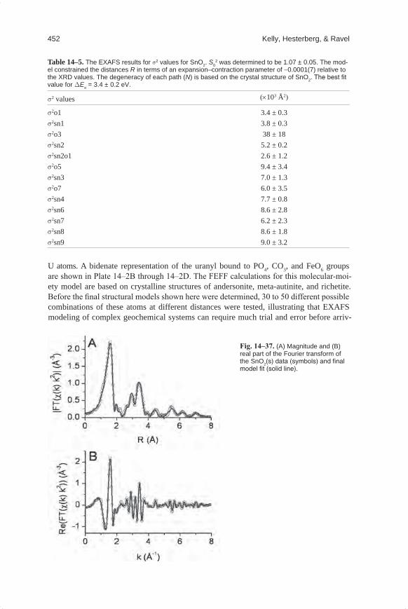
452 Kelly, Hesterberg, & Ravel
U atoms. A bidenate representation of the uranyl bound to PO4, CO3, and FeO6 groups are shown in Plate 14–2B through 14–2D. The FEFF calculations for this molecular-moi-ety model are based on crystalline structures of andersonite, meta-autinite, and richetite. Before the final structural models shown here were determined, 30 to 50 different possible combinations of these atoms at different distances were tested, illustrating that EXAFS modeling of complex geochemical systems can require much trial and error before arriv-
Table14–5.The EXAFS results for s2 values for SnO2. S02 was determined to be 1.07 ± 0.05. The mod-
el constrained the distances R in terms of an expansion–contraction parameter of −0.0001(7) relative to the XRD values. The degeneracy of each path (N) is based on the crystal structure of SnO2. The best fit value for DEo = 3.4 ± 0.2 eV.
s2 values (×103 Å2)
s2o1 3.4 ± 0.3s2sn1 3.8 ± 0.3s2o3 38 ± 18s2sn2 5.2 ± 0.2s2sn2o1 2.6 ± 1.2s2o5 9.4 ± 3.4s2sn3 7.0 ± 1.3s2o7 6.0 ± 3.5s2sn4 7.7 ± 0.8s2sn6 8.6 ± 2.8s2sn7 6.2 ± 2.3s2sn8 8.6 ± 1.8s2sn9 9.0 ± 3.2
Fig. 14–37. (A) Magnitude and (B) real part of the Fourier transform of the SnO2(s) data (symbols) and final model fit (solid line).
Mineralogical Methods.indb 452 2/15/2008 2:37:46 PM
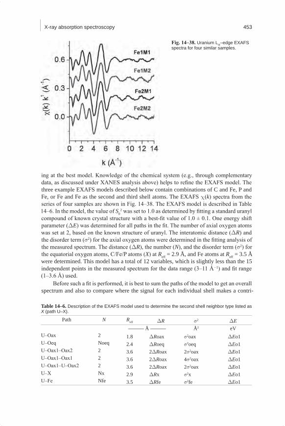
X-ray absorption spectroscopy 453
ing at the best model. Knowledge of the chemical system (e.g., through complementary data, as discussed under XANES analysis above) helps to refine the EXAFS model. The three example EXAFS models described below contain combinations of C and Fe, P and Fe, or Fe and Fe as the second and third shell atoms. The EXAFS c(k) spectra from the series of four samples are shown in Fig. 14–38. The EXAFS model is described in Table 14–6. In the model, the value of S0
2 was set to 1.0 as determined by fitting a standard uranyl compound of known crystal structure with a best-fit value of 1.0 ± 0.1. One energy shift parameter (DE) was determined for all paths in the fit. The number of axial oxygen atoms was set at 2, based on the known structure of uranyl. The interatomic distance (DR) and the disorder term (s2) for the axial oxygen atoms were determined in the fitting analysis of the measured spectrum. The distance (DR), the number (N), and the disorder term (s2) for the equatorial oxygen atoms, C/Fe/P atoms (X) at Reff = 2.9 Å, and Fe atoms at Reff = 3.5 Å were determined. This model has a total of 12 variables, which is slightly less than the 15 independent points in the measured spectrum for the data range (3–11 Å-1) and fit range (1–3.6 Å) used.
Before such a fit is performed, it is best to sum the paths of the model to get an overall spectrum and also to compare where the signal for each individual shell makes a contri-
Fig. 14–38. Uranium LIII–edge EXAFS spectra for four similar samples.
Table14–6.Description of the EXAFS model used to determine the second shell neighbor type listed as X (path U–X).
Path N Reff DR s2 DE——— Å ——— Å2 eV
U–Oax 2 1.8 DRoax s2oax DEo1U–Oeq Noeq 2.4 DRoeq s2oeq DEo1U–Oax1–Oax2 2 3.6 2DRoax 2s2oax DEo1U–Oax1–Oax1 2 3.6 2DRoax 4s2oax DEo1U–Oax1–U–Oax2 2 3.6 2DRoax 2s2oax DEo1U–X Nx 2.9 DRx s2x DEo1U–Fe Nfe 3.5 DRfe s2fe DEo1
Mineralogical Methods.indb 453 2/15/2008 2:37:47 PM
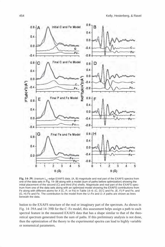
454 Kelly, Hesterberg, & Ravel
bution to the EXAFS structure of the real or imaginary part of the spectrum. As shown in Fig. 14–39A and 14–39B for the C–Fe model, this assessment helps assign a path to each spectral feature in the measured EXAFS data that has a shape similar to that of the theo-retical spectrum generated from the sum of paths. If this preliminary analysis is not done, then the optimization of the theory to the experimental spectra can lead to highly variable or nonsensical parameters.
Fig. 14–39. Uranium LIII–edge EXAFS data. (A, B) magnitude and real part of the EXAFS spectra from one of the data sets in Fig. 14–38 along with a model (sum of paths before optimization) showing the initial placement of the second (C) and third (Fe) shells. Magnitude and real part of the EXAFS spec-trum from one of the data sets along with an optimized model showing the EXAFS contributions from Fe along with different atoms for X (C, P, or Fe) in Table 14–6: (C, D) C and Fe, (E, F) P and Fe, and (G, H) Fe and Fe. The contribution to the model from the U–Fe and U–X paths are shown as lines beneath the data.
Mineralogical Methods.indb 454 2/15/2008 2:37:48 PM
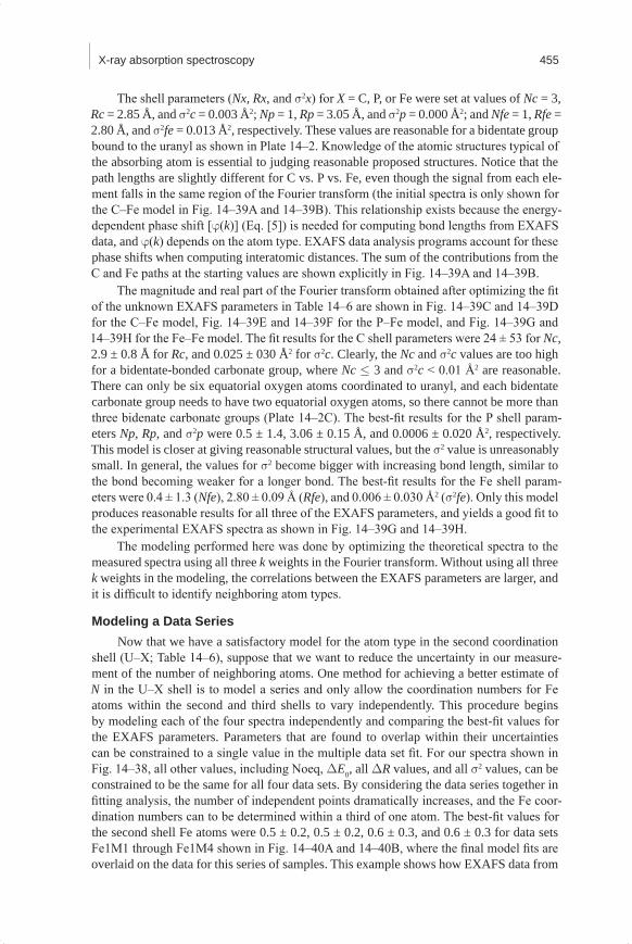
X-ray absorption spectroscopy 455
The shell parameters (Nx, Rx, and s2x) for X = C, P, or Fe were set at values of Nc = 3, Rc = 2.85 Å, and s2c = 0.003 Å2; Np = 1, Rp = 3.05 Å, and s2p = 0.000 Å2; and Nfe = 1, Rfe = 2.80 Å, and s2fe = 0.013 Å2, respectively. These values are reasonable for a bidentate group bound to the uranyl as shown in Plate 14–2. Knowledge of the atomic structures typical of the absorbing atom is essential to judging reasonable proposed structures. Notice that the path lengths are slightly different for C vs. P vs. Fe, even though the signal from each ele-ment falls in the same region of the Fourier transform (the initial spectra is only shown for the C–Fe model in Fig. 14–39A and 14–39B). This relationship exists because the energy-dependent phase shift [j(k)] (Eq. [5]) is needed for computing bond lengths from EXAFS data, and j(k) depends on the atom type. EXAFS data analysis programs account for these phase shifts when computing interatomic distances. The sum of the contributions from the C and Fe paths at the starting values are shown explicitly in Fig. 14–39A and 14–39B.
The magnitude and real part of the Fourier transform obtained after optimizing the fit of the unknown EXAFS parameters in Table 14–6 are shown in Fig. 14–39C and 14–39D for the C–Fe model, Fig. 14–39E and 14–39F for the P–Fe model, and Fig. 14–39G and 14–39H for the Fe–Fe model. The fit results for the C shell parameters were 24 ± 53 for Nc, 2.9 ± 0.8 Å for Rc, and 0.025 ± 030 Å2 for s2c. Clearly, the Nc and s2c values are too high for a bidentate-bonded carbonate group, where Nc £ 3 and s2c < 0.01 Å2 are reasonable. There can only be six equatorial oxygen atoms coordinated to uranyl, and each bidentate carbonate group needs to have two equatorial oxygen atoms, so there cannot be more than three bidenate carbonate groups (Plate 14–2C). The best-fit results for the P shell param-eters Np, Rp, and s2p were 0.5 ± 1.4, 3.06 ± 0.15 Å, and 0.0006 ± 0.020 Å2, respectively. This model is closer at giving reasonable structural values, but the s2 value is unreasonably small. In general, the values for s2 become bigger with increasing bond length, similar to the bond becoming weaker for a longer bond. The best-fit results for the Fe shell param-eters were 0.4 ± 1.3 (Nfe), 2.80 ± 0.09 Å (Rfe), and 0.006 ± 0.030 Å2 (s2fe). Only this model produces reasonable results for all three of the EXAFS parameters, and yields a good fit to the experimental EXAFS spectra as shown in Fig. 14–39G and 14–39H.
The modeling performed here was done by optimizing the theoretical spectra to the measured spectra using all three k weights in the Fourier transform. Without using all three k weights in the modeling, the correlations between the EXAFS parameters are larger, and it is difficult to identify neighboring atom types.
Modeling a Data SeriesNow that we have a satisfactory model for the atom type in the second coordination
shell (U–X; Table 14–6), suppose that we want to reduce the uncertainty in our measure-ment of the number of neighboring atoms. One method for achieving a better estimate of N in the U–X shell is to model a series and only allow the coordination numbers for Fe atoms within the second and third shells to vary independently. This procedure begins by modeling each of the four spectra independently and comparing the best-fit values for the EXAFS parameters. Parameters that are found to overlap within their uncertainties can be constrained to a single value in the multiple data set fit. For our spectra shown in Fig. 14–38, all other values, including Noeq, DE0, all DR values, and all s2 values, can be constrained to be the same for all four data sets. By considering the data series together in fitting analysis, the number of independent points dramatically increases, and the Fe coor-dination numbers can to be determined within a third of one atom. The best-fit values for the second shell Fe atoms were 0.5 ± 0.2, 0.5 ± 0.2, 0.6 ± 0.3, and 0.6 ± 0.3 for data sets Fe1M1 through Fe1M4 shown in Fig. 14–40A and 14–40B, where the final model fits are overlaid on the data for this series of samples. This example shows how EXAFS data from
Mineralogical Methods.indb 455 2/15/2008 2:37:48 PM
456 Kelly, Hesterberg, & Ravel
a chemically similar set of samples improves statistical power when performing EXAFS fitting analysis, once a reasonable structural model has been developed.
EXAFS Modeling of Complex, Multicomponent SystemsOne of the principle objectives of this chapter is to develop generalized approaches
for modeling a series of spectra that include trace elements within soil samples. Here we outline one approach based on the analysis methods explained in the examples. If it is ex-pected that the trace element interacts strongly with Fe (e.g., in an Fe oxide) or some other metal within the soil, it is recommended that absorption spectra are collected for both ele-ments to develop a self-consistent structural model for both metals. However, recognize that if the major elemental concentration in the sample is much greater than that of trace elements, then the signal from the majority absorber will contain only a fraction of the mi-nority atoms in its nearby coordination shells.
The first step is to decide which standard spectra should be collected. These could be fine-grained metal powder or minerals of known crystalline structure mixed with BN. It is common to use the standard with a known crystal structure to determine an appropriate value for S0
2. Other commercially available minerals standards might be included to help gain insight into the soil spectra. Many of these standard spectra are freely available from
Fig.14–40. Magnitude and real part of the Fourier transform of the U LIII–edge EXAFS data (open circles) and best-fit model (lines) optimized for each spectrum in the entire data series.
Mineralogical Methods.indb 456 2/15/2008 2:37:48 PM
X-ray absorption spectroscopy 457
the EXAFS standards database (Newville et al., 1999a). Additional synthesized standards should also be considered.
Once the data have been collected and processed, a generalized modeling approach is needed. One of the most useful initial approaches is to compare the measured spectra to each other without any theoretical models. Comparison of XANES and EXAFS c(k) spec-tra are valuable for determining similarities and differences. As shown in Fig. 14–38, these spectra were a subset of the initially collected data, but were determined from comparison of the c(k) spectra to be very similar. The next step usually involves processing each of the spectra so that the usable k range is determined (Fig. 14–26). Then the Fourier transform of the spectrum with different k weights (of 1, 2, and 3) can be compared. The spectra are scaled so that the first peak height is about the same for all three spectra. As shown in Fig. 14–25, differences in second and third shell atom types as compared with the first shell types can be determined from relative changes in the Fourier transform processed with dif-ferent k weights. General trends for each spectrum and between spectra can give insights into how the species are related within each of the samples.
The next step is to model the standard spectra that have known crystal structures. These models can be built, as shown with SnO2 in the above sections. From these models, we gain insight to the typical values of EXAFS parameters (N, DR, s2, DE, S0
2) for dif-ferent species.
The EXAFS spectra for the soil samples with unknown crystalline or noncrystalline structures can be modeled with simple molecular-moiety models similar to those described above in the example of “Determining a Second Shell Atom Type” (Plate 14–2). In this step the simplest model that describes the EXAFS data for all three k weights is determined. The structural parameters of this model are compared with the known structural models from the previous step to gain additional insight into the species present in the soil sample.
Once a simple model has been determined for the soil sample, the atomic distribu-tion can be compared with the known crystal structures. From this comparison, it might be possible that one of the known crystal structural models can be used to model the spectra from the undefined species, or the known crystal structural model may need to be slightly modified to describe the species within the sample. Possible methods for using the crystal structural model to describe an adsorbed or coprecipitated species include fixing all of the EXAFS parameters from the crystalline model, then multiplying all paths in the soil sam-ple by one additional fractional parameter ( f ) so that the degeneracy of each path is given by f N, where N is the degeneracy of the path determined from the crystal structure. This model can be used to test whether the measured spectra represents a fractional component of the crystalline mineral phase in the sample (Bare et al., 2005). Another modeling ap-proach adds an additional constant disorder term (s2
d) to each of the paths. This approach would test the measured spectra for a fractional component that is more disordered than the crystal structure of the standard. It is also possible that the unknown species includes a fraction of poorly crystalline particles. If so, then the second and third shell N values will be too large compared with the first shell values. These coordination numbers could be relaxed (e.g., use fN only for the higher-shell paths) for modeling the unknown species. In addition, nanoparticles can cause the interatomic distances to become smaller than for the bulk structure, so that these parameters could also need adjustment, as in O’Loughlin et al. (2003).
It is also possible that the major and minor element spectra may be related to each other in some way so that the spectra from both edges can be co-refined. In particular, the Major–Minor path from the major element spectra should have the same distance and s2 values as the Minor–Major path from the minor element spectra. Physically the Minor–
Mineralogical Methods.indb 457 2/15/2008 2:37:48 PM
458 Kelly, Hesterberg, & Ravel
Major pairs in the sample are represented by only one distance and one s2 value. They do not depend on the absorber atom. The EXAFS spectrum is the average local atomic distribution of all the absorber atoms within the sample. It is possible, for example, that with only one minor-element atom for every 50 major-element atoms within a sample, the major-element edge spectra would not detect the minor-element signal. Nevertheless, it is best to make the measurement and then determine if there is a measurable effect. Even in this case, the major-element spectrum is useful for describing the host material with which the minor-element might be associated (adsorbed or coprecipitated), particularly if X-ray diffraction cannot be used to characterize crystalline phases in the soil sample.
There are many different models that can be used to accurately describe one EXAFS spectrum. The most robust model uses the fewest variables and is constrained to make physical sense for the system. If the model is based on a known crystal structure, then the model might include many paths but only a few variables. If the model is based on molecu-lar-moiety approach, then the model might include only a few of the most important paths with a relatively large number of variables. Both of these methods for building EXAFS models can be appropriate for different questions proposed by the scientific objectives be-hind the measurements. Understanding the chemical species possible for a given element and its geochemical properties within the sample of interest are fundamental to building robust EXAFS models.
DATA REPORTINGThe International XAFS Society (IXS) has formed the IXS Standards and Criteria
Subcommittee to generate criteria for reporting spectral analyses. These documents are available at www.i-x-s.org. Following is a brief summary of the information that should be presented within a manuscript when reporting XAFS analysis.
Data collection procedures need to be reported or referenced. The acknowledgment section should include the funding source for the synchrotron, and the methods section should include a reference for the beamline. Parameters pertaining to the energy selection method (monochromator type, monochromator slits), harmonic X-ray elimination (detune percentage, type of mirror), focusing optics (KB mirrors, zone plates), X-ray filters (for flu-orescence measurements), and detector types (ionization chambers, solid-state detectors), including the fill gases for ionization chambers, are relevant for almost all experiments. The profile (spot size, shape) of the X-ray beam incident on the sample is usually relevant. Key sample parameters are the type of sample, sample preparation methods, and the mode of data collection (transmission or fluorescence).
The data processing procedures (deglitching, smoothing, alignment, normalization, background removal, fitting) should be given, including references to software packages written by your peers for your benefit. The structural model should be described, including a method for accounting for each of the EXAFS parameters (N, R, s2, S0
2, DE0) for each path included in the model. The fitting results for all parameters determined in the fit to the measured spectra should be given with uncertainties, and those uncertainties should be de-termined from the optimization of each parameter. Generalized uncertainties (such as those stated in a table heading) are not meaningful. The total number of variables determined in the model fit and the number of independent points in the measured spectrum, includ-ing the data range (Dk) and the fit range (DR) should be given. If several model fits are compared, then the procedure used to determine the quality of the model needs to be given or referenced, including how to determine the significance of two different statistical mea-surements of fit quality. Plots of the EXAFS data overlaid with the model fit must be shown.
Mineralogical Methods.indb 458 2/15/2008 2:37:48 PM
X-ray absorption spectroscopy 459
The EXAFS c(k) spectra (data and fit) alone is sufficient, but it is better to also include at least one part (magnitude, real, or imaginary) of the Fourier transform. Alternatively, both the magnitude with either the real or imaginary parts of the Fourier transform are sufficient. All EXAFS data spectra should start at k or R of 0 and end beyond the fitting range used in the analysis. The EXAFS spectra should be labeled with values on both axes, and the axis labels should include the k weight of the spectra shown.
SUMMARYX-ray absorption spectroscopy is a powerful tool for characterizing both crystalline
and non-crystalline chemical and mineralogical forms (species) of many different elements occurring in trace or abundant concentrations in soil and mineral samples. This technique complements X-ray diffraction analysis of the more abundant soil minerals and is sensi-tive to minority components undetectable by X-ray diffraction. Theories of both XANES and EXAFS spectra have been developed to the point where quantitative information on average local molecular bonding can be derived. Because XANES and EXAFS features arise from different physical phenomena, each of these regions of the XAS spectrum can be treated as independent (and complementary) sources of structural information for chemical species. Results from both XANES and EXAFS must be consistent if a given structural model is accurate.
A major advantage of XAS over other analytical techniques for soils is its applicabil-ity to whole (moist) soil samples with little or no pretreatment requirements. Care must be taken in sample preservation and preparation for XAS analysis to ensure that the molecular state of the element of interest is not significantly altered between the time of sampling and the time of data collection at a synchrotron facility. Presently, the greatest limitation to fully quantifying the chemical species of an element in a complex soil matrix is our ability to select and synthesize or isolate purified standards that have molecular-scale properties identical to the species of an element expected in a soil. Nevertheless, coupling synchro-tron techniques such as micro-X-ray diffraction and micro-XAS with bulk-sample XAS analysis to identify the structural features that make soil minerals and noncrystalline solids unique is a powerful tool.
AcknowledgmentsThe authors acknowledge Kimberly Hutchison, Amanda Morris, and Yu-Ting Liu for
laboratory work associated with some of the data presented, and Dr. Suzanne Beauchemin for insightful comments on the PCA section. We acknowledge Kenneth Kemner, Mandy Michalsen, and Simon Bare for some of the example spectra. Support for SDK and BR provided by the Environmental Remediation Science Program, Office of Biological and Environmental Research, Office of Science, U.S. Department of Energy (DOE), under con-tract W-31-109-Eng-38 and for DH provided by the North Carolina Agricultural Research Service (NC-ARS). This work was carried out in part at MRCAT at the Advanced Photon Source (APS) at Argonne National Laboratory, and at Beamlines X-11A, X-11B, and X-15B at the National Synchrotron Light Source (NSLS), Brookhaven National Laboratory. MRCAT operations are supported by the Department of Energy and the MRCAT member institutions. Use of the APS and NSLS is supported by the U.S. Department of Energy, Office of Science, Office of Basic Energy Sciences, under Contract Numbers DE-AC02-06CH11357 and DE-AC02-98CH10886.
Mineralogical Methods.indb 459 2/15/2008 2:37:48 PM
460 Kelly, Hesterberg, & Ravel
REFERENCESAllen, P.G., J.J. Bucher, D.L. Clark, N.M. Edelstein, S.A. Ekberg, J.W. Gohdes, E.A. Hudson, N.
Kaltsoyannis, W.W. Lukens, M.P. Neu, P.D. Palmer, T. Reich, D.K. Shuh, C.D. Tait, and B.D. Zwick. 1995. Multinuclear NMR, Raman, EXAFS, and X-ray-diffraction studies of uranyl car-bonate complexes in near-neutral aqueous-solution: X-ray Structure of [C(NH2)3]6[(UO2)3(CO3)6]6.5H2O. Inorg. Chem. 34:4797–4807.
Ankudinov, A.L., A.I. Nesvizhskii, and J.J. Rehr. 2003. Dynamic screening effects in x-ray absorption spectra. Phys. Rev. B 67:115120.
Ankudinov, A.L., B. Ravel, J.J. Rehr, and S.D. Conradson. 1998. Real-space multiple-scattering calcu-lation and interpretation of X-ray absorption near-edge structure. Phys. Rev. B 58:7565–7576.
Bare, S.R., S.D. Kelly, W. Sinkler, J.J. Low, F.S. Modica, S. Valencia, A. Corma, and L.T. Nemeth. 2005. Uniform catalytic site in Sn-beta-zeolite determined using X-ray absorption fine structure. J. Am. Chem. Soc. 127:12924–12932.
Bartlett, R.J., and B.R. James. 1993. Redox chemistry of soils. Adv. Agron. 50:151–208.Beauchemin, S., D. Hesterberg, and M. Beauchemin. 2002. Principal component analysis approach
for the modeling of sulfur K-XANES spectra of humic acid. Soil Sci. Soc. Am. J. 66:83–91.Beauchemin, S., D. Hesterberg, J. Chou, M. Beauchemin, R.R. Simard, and D.E. Sayers. 2003.
Speciation of phosphorus in P-enriched agricultural soils using XANES spectroscopy and chem-ical fractionation. J. Environ. Qual. 32:1809–1819.
Benfatto, M., P. D’Angelo, S. Della Longa, and N.V. Pavel. 2002. Evidence of distorted fivefold coor-dination of the Cu2+ aqua ion from an x-ray-absorption spectroscopy quantitative analysis. Phys. Rev. B 65: Art. No. 174205.
Bertsch, P.M., and D.B. Hunter. 2001. Applications of synchrotron-based X-ray microprobes. Chem. Rev. 101:1809–1842.
Bertsch, P.M., D.B. Hunter, S.R. Sutton, S. Bajt, and M.R. Rivers. 1994. In situ chemical speciation of uranium in soils and sediments using micro X-ray absorption spectroscopy. Environ. Sci. Technol. 28:980–984.
Bevington, P.R., and D.K. Robinson. 1992. Data reduction and error analysis for the physical sciences. 2nd ed. McGraw-Hill, New York.
Brillouin, L. 1962. Science and information theory. Academic Press, New York.Brown, G.E., Jr. 1990. Spectroscopic studies of chemisorption reaction mechanisms at oxide–water
interfaces. p. 309–364. In M.F. Hochella, Jr. and A.F. White (ed.) Mineral–water interface geo-chemistry. Reviews in Mineralogy 23. Mineralogical Soc. of America, Washington, DC.
Brown, G.E., and G.A. Parks. 2001. Sorption of trace elements on mineral surfaces: Modern perspec-tives from spectroscopic studies, and comments on sorption in the marine environment. Int. Geol. Rev. 43:963–1073.
Brown, G.E., and N. Sturchio. 2002. An overview of synchrotron radiation applications to low tem-perature geochemistry and environmental sciences. p. 1–115. In P.A. Fenter et al. (ed.) 2002. Applications of synchrotron radiation in low-temperature geochemistry and environmental sci-ence. Reviews in Mineralogy and Geochemistry 49. Mineralogical Soc. Am., Washington, DC.
Calvin, S., E.E. Carpenter, B. Ravel, V.G. Harris, and S.A. Morrison. 2002. Multiedge refinement of extended X-ray-absorption fine structure of manganese zinc ferrite nanoparticles. Phys. Rev. B 66: Art. No. 224405.
Compton, A.H.A. 1923. Quantum theory of the scattering of X-rays by light elements. Phys. Rev. 21:483–502.
Cross, J.O., and A.I. Frenkel. 1998. Use of scattered radiation for absolute energy calibration. Rev. Sci. Instrum. 70:38–40.
Cullity, B.D. 1978. Elements of X-ray diffraction. Addison-Wesley, Reading, MA.Davis, L.E. 1976. Handbook of Auger electron spectroscopy: A reference book of standard data
for identification and interpretation of Auger electron spectroscopy data. Physical Electronics Industries, Inc., Edina, MN.
de Groot, F. 2005. Multiplet effects in X-ray spectroscopy. Coord. Chem. Rev. 249:31–63.Duff, M.C., D.B. Hunter, I.R. Triay, P.M. Bertsch, D.T. Reed, S.R. Sutton, G. Shea-McCarthy, J.
Kitten, P. Eng, S.J. Chipera, and D.T. Vaniman. 1999. Mineral associations and average oxida-tion states of sorbed Pu on tuff. Environ. Sci. Technol. 33:2163–2169.
Elam, W.T., B. Ravel, and J.R. Sieber. 2002. A new atomic database for X-ray spectroscopic calcula-tions. Radiat. Phys. Chem. 63:121–128.
Felmy, A.R., D.C. Girvin, and E.A. Jenne. 1984. MINTEQ—A computer program for computing aqueous equilibria. Rep. by Battelle Pacific Northwest Laboratories for the USEPA, Athens, GA.
Fendorf, S.E. 1999. Fundamental aspects and applications of x-ray absorption spectroscopy in clay and soil science. p. 19–67 In D.G. Schulze et al. (ed.) Synchrotron methods in clay science. CMS
Mineralogical Methods.indb 460 2/15/2008 2:37:49 PM
X-ray absorption spectroscopy 461
Workshop Lectures, Vol. 9. Clay Minerals Society, Aurora, CO.Fendorf, S.E., and D.L. Sparks. 1996. X-ray absorption fine structure spectroscopy. p. 357–375. In
D.L. Sparks (ed.) Methods of soil analysis. Part 3. SSSA Book Ser. 5. SSSA, Madison, WI.Fendorf, S.E., D.L. Sparks, G.M. Lamble, and M.J. Kelley. 1994. Applications of x-ray absorption
fine structure spectroscopy to soils. Soil Sci. Soc. Am. J. 58:1583–1595.Fenter, P.A., M.L. Rivers, N.C. Sturchio, and S.R. Sutton (ed.) 2002. Applications of synchrotron
radiation in low-temperature geochemistry and environmental science. Reviews in Mineralogy and Geochemistry 49. Mineralogical Soc. Am., Washington, DC.
Fernández-García, M., C.M. Alvarez, and G.L. Haller. 1995. XANES-TPR study of Cu-Pd bimetallic catalysts: Application of factor analysis. J. Phys. Chem. 99:12565–12569.
Frenkel, A.I., C.W. Hills, and R.G.A. Nuzzo. 2001. A view from the inside: Complexity in the atomic scale ordering of supported metal nanoparticles. J. Phys. Chem. B 105:12689–12703.
Frenkel, A.I., E.A. Stern, A. Voronel, M. Qian, and M. Newville. 1994. Solving the structure of disor-dered mixed salts. Phys. Rev. B 49:11662–11674.
Frenkel, A.I., F.M. Wang, S. Kelly, R. Ingalls, D. Haskel, E.A. Stern, and Y. Yacoby. 1997. Local structural changes in KNbO3 under high pressure. Phys. Rev. B 56:10869–10877.
Gustafsson, J.P. 2007. Software download page for Visual Minteq. Available at http://www.lwr.kth.se/English/OurSoftware/vminteq/ (accessed 31 July 2007, verified 17 Dec. 2007).
Haskel, D., J.C. Lang, Z. Islam, A. Cady, G. Srajer, M. van Veenendaal, and P.C. Canfield. 2005. Atomic origin of magnetocrystalline anisotropy in Nd2Fe14B. Phys. Rev. Lett. 95: Art. No. 217207.
Heald, S.M. 1988a. Design of an EXAFS experiment. p. 87–118. In D.C. Koningsberger and R. Prins (ed.) X-ray absorption: Principles, applications, techniques of EXAFS, SEXAFS and XANES. John Wiley & Sons, New York.
Heald, S.M. 1988b. EXAFS with synchrotron radiation. p. 119–161. In D.C. Koningsberger and R. Prins (ed.) X-ray absorption: Principles, applications, techniques of EXAFS, SEXAFS and XANES. John Wiley & Sons, New York.
Hesterberg, D., D.E. Sayers, W. Zhou, G.M. Plummer, and W.P. Robarge. 1997. X-ray absorption spectroscopy of lead and zinc speciation in a contaminated groundwater aquifer. Environ. Sci. Technol. 31:2840–2846.
Hesterberg, D., W. Zhou, K.J. Hutchison, and D.E. Sayers. 2001. Bonding of Hg(II) to reduced or-ganic sulfur in humic acid as affected by S/Hg ratio. Environ. Sci. Technol. 35:2741–2745.
Joly, Y. 2001. X-ray absorption near edge structure calculations beyond the muffin-tin approximation. Phys. Rev. B 63:125120–125129.
Kelly, S., R. Ingalls, F. Wang, B. Ravel, and D. Haskel. 1998. X-ray-absorption fine-structure study of the B1-to-B2 phase transition in RbCl. Phys. Rev. B 57:7543–7550.
Kelly, S.D., K.M. Kemner, J.B. Fein, D.A. Fowle, M.I. Boyanov, B.A. Bunker, and N. Yee. 2002. X-ray absorption fine structure determination of pH-dependent U-bacterial cell wall interactions. Geochim. Cosmochim. Acta 66:3855–3871.
Kelly, S.D., E.T. Rasbury, S. Chattopardhyay, A.J. Kropf, and K.M. Kemnner. 2006. Evidence of a stable uranyl site in ancient organic-rich calcite. Environ. Sci. Technol. 40:2262–2268.
Kelly, S.D., E.A. Stern, and R. Ingalls. 2001. Determining crystalline atomic positions using XAFS, a new addition to the UWXAFS analysis package. J. Synchrotron Radiat. 8:311–313.
Kemner, K.M., J. Kropf, and B.A. Bunker. 1994. A low-temperature total electron yield detector for X-ray absorption fine structure spectra. Rev. Sci. Instrum. 65:3667–3669.
Khare, N., D. Hesterberg, S. Beauchemin, and S.L. Wang. 2004. XANES determination of adsorbed phosphate distribution between ferrihydrite and boehmite in mixtures. Soil Sci. Soc. Am. J. 68:460–469.
Khare, N., D. Hesterberg, and J.D. Martin. 2005. Investigating phosphate surface precipitation in single and binary mixtures of Fe- and Al-oxide minerals using XANES. Environ. Sci. Technol. 39:2152–2160.
Koningsberger, D.C., and R. Prins (ed.) 1988. X-ray absorption: Principles, applications, techniques of EXAFS, SEXAFS and XANES. John Wiley & Sons, New York.
Li, G.G., F. Bridges, and C.H. Booth. 1995. X-ray absorption fine-structure standards—A comparison of experiment and theory. Phys. Rev. B 52:6332–6348.
Lide, D.R. (ed.) 2003. CRC handbook of chemistry and physics. 84th ed. CRC Press, Boca Raton, FL.
Malinowski, E.R. 2002. Factor analysis in chemistry. 3rd ed. John Wiley & Sons, New York.Manceau, A., L. Charlet, M.C. Boisset, B. Didier, and L. Spadini. 1992. Sorption and speciation of
heavy metals on hydrous Fe and Mn oxides. From microscopic to macroscopic. Appl. Clay Sci. 7:201–223.
Mineralogical Methods.indb 461 2/15/2008 2:37:49 PM
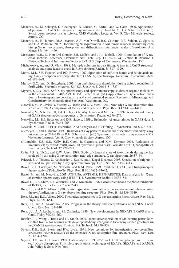
462 Kelly, Hesterberg, & Ravel
Manceau, A., M. Schlegel, D. Chateigner, B. Lanson, C. Bartoli, and W. Gates. 1999. Application of polarized EXAFS to fine-grained layered minerals. p. 69–114. In D.G. Schulze et al. (ed.) Synchrotron methods in clay science. CMS Workshop Lectures, Vol. 9. Clay Minerals Society, Aurora, CO.
Manceau, A., N. Tamura, M.A. Marcus, A.A. MacDowell, R.S. Celestre, R.E. Sublett, G. Sposito, and H.A. Padmore. 2002. Deciphering Ni sequestration in soil ferromanganese nodules by com-bining X-ray fluorescence, absorption, and diffraction at micrometer scales of resolution. Am. Miner. 87:1494–1499.
McMaster, W.H., N. Kerr Del Grande, J.H. Mallett, and J.H. Hubbell. 1969. Compilation of X-ray cross sections. Lawrence Livermore Natl. Lab. Rep. UCRL-50174, Section II Revision I. National Technical Information Services L-3. U.S. Dep. of Commerce, Washington, DC.
Michalowicz, A., and G. Vlaic. 1998. Multiple solutions in data fitting: A trap in EXAFS structural analysis and some ideas to avoid it. J. Synchrotron Radiat. 5:1317–1320.
Morra, M.J., S.E. Fendorf, and P.D. Brown. 1997. Speciation of sulfur in humic and fulvic acids us-ing X-ray absorption near-edge structure (XANES) spectroscopy. Geochim. Cosmochim. Acta 61:683–688.
Murray, G.C., and D. Hesterberg. 2006. Iron and phosphate dissolution during abiotic reduction of ferrihydrite–boehmite mixtures. Soil Sci. Soc. Am. J. 70:1318–1327.
Myneni, S.C.B. 2002. Soft X-ray spectroscopy and spectromicroscopy studies of organic molecules in the environment. p. 485–579. In P.A. Fenter et al. (ed.) Applications of synchrotron radia-tion in low-temperature geochemistry and environmental science. Reviews in Mineralogy and Geochemistry 49. Mineralogical Soc. Am., Washington, DC.
Newville, M., P. Livins, Y. Yacoby, J.J. Rehr, and E.A. Stern. 1993. Near-edge X-ray-absorption fine structure of Pb: A comparison of theory and experiment. Phys. Rev. B 47:14126–14131.
Newville, M., S.A. Carroll, P.A. O’Day, G.A. Waychunas, and M. Ebert. 1999a. A web-based library of XAFS data on model compounds. J. Synchrotron Radiat. 6:276–277.
Newville, M., B.I. Boyanov, and D.E. Sayers. 1999b. Estimation of uncertainties in XAFS data. J. Synchrotron Radiat. 6:264–265.
Newville, M. 2001. IFEFFIT: Interactive EXAFS analysis and FEFF fitting. J. Synchroton Rad. 8:322–324.Niemeyer, J., and J. Thieme. 1999. Reactions of clay particles in aqueous dispersions studied by x-ray
microscopy. p. 207–239. In D.G. Schulze et al. (ed.) Synchrotron methods in clay science. CMS Workshop Lectures, Vol. 9. Clay Minerals Society, Aurora, CO.
O’Loughlin, E.J., S.D. Kelly, R.E. Cook, R. Csencsits, and K.M. Kemner. 2003. Reduction of uranium(VI) by mixed iron(II)/iron(III) hydroxide (green rust): Formation of UO2 nanoparticles. Environ. Sci. Technol. 37:721–727.
Osán, J.B., S. Török, and K.W. Jones. 1997. Study of chemical state of toxic metals during the life cycle of fly ash using X-ray absorption near-edge structure. X-ray Spectrom. 26:37–44.
Prietzel, J., J. Thieme, U. Neuhäusler, J. Susini, and I. Kögel-Knabner. 2003. Speciation of sulphur in soils and soil particles by X-ray spectromicroscopy. Eur. J. Soil Sci. 54:423–433.
Ravel, B., E. Cockayne, M. Newville, and K.M. Rabe. 1999. Combined EXAFS and first-principles theory study of Pb1-xGexTe. Phys. Rev. B 60:14632–14642.
Ravel, B., and M. Newville. 2005. ATHENA, ARTEMIS, HEPHAESTUS: Data analysis for X-ray absorption spectroscopy using IFEFFIT. J. Synchrotron Radiat. 12:537–541.
Ravel, B., E.A. Stern, R.I. Vedrinskii, and V. Kraizman. 1998. Local structure and the phase transitions of BaTiO3. Ferroelectrics 206:407–430.
Rehr, J.J., and R.C. Albers. 1990. Scattering-matrix formulation of curved-wave multiple-scattering theory: Application to X-ray-absorption fine structure. Phys. Rev. B 41:8139–8149.
Rehr, J.J., and R.C. Albers. 2000. Theoretical approaches to X-ray absorption fine structure. Rev. Mod. Phys. 72:621–654.
Rehr, J.J., and A. Ankudinov. 2005. Progress in the theory and interpretations of XANES. Coord. Chem. Rev. 249:131–140.
Rehr, J.J., A. Ankudinov, and S.I. Zabinsky. 1998. New developments in NEXAFS/EXAFS theory. Catal. Today 39:263–269.
Ressler, T., J. Wong, J. Roos, and I.L. Smith. 2000. Quantitative speciation of Mn-bearing particulates emitted from autos burning methylcyclopentadienyl)manganese tricarbonyl-added gasolines us-ing XANES spectroscopy. Environ. Sci. Technol. 34:950–958.
Sayers, D.E., E.A. Stern, and F.W. Lytle. 1971. New technique for investigating non-crystalline structures: Fourier analysis of the extended X-ray absorption fine structure. Phys. Rev. Lett. 27:1204–1207.
Sayers, D.E., and B. Bunker. 1988. Data analysis. p. 211–256. In D.C. Koningsberger and R. Prins (ed.) X-ray absorption: Principles, applications, techniques of EXAFS, SEXAFS and XANES. John Wiley & Sons, New York.
Mineralogical Methods.indb 462 2/15/2008 2:37:49 PM
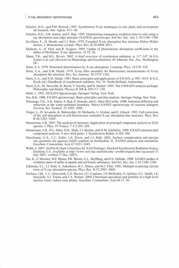
X-ray absorption spectroscopy 463
Schulze, D.G., and P.M. Bertsch. 1995. Synchrotron X-ray techniques in soil, plant, and environmen-tal research. Adv. Agron. 55:1–66.
Schulze, D.G., S.R. Sutton, and S. Bajt. 1995. Determining manganese oxidation state in soils using x-ray absorption near-edge structure (XANES) spectroscopy. Soil Sci. Soc. Am. J. 59:1540–1548.
Sevillano, E., H. Meuth, and J.J. Rehr. 1979. Extended X-ray absorption fine structure Debye-Waller factors. I. Monoatomic crystals. Phys. Rev. B 20:4908–4911.
Shaltout, A., H. Ebel, and R. Svagera. 2005. Update of photoelectric absorption coefficients in the tables of McMaster. X-ray Spectrom. 35:52–56.
Sham, T.K., and M.L. Rivers. 2002. A brief overview of synchrotron radiation. p. 117–147. In P.A. Fenter et al. (ed.) Reviews in Mineralogy and Geochemistry 49. Mineral. Soc. Am., Washington, DC.
Stern, E.A. 1978. Structural determination by X-ray absorption. Contemp. Phys. 19:239–310.Stern, E.A., and S.M. Heald. 1979. X-ray filter assembly for fluorescence measurements of X-ray
absorption file structure. Rev. Sci. Instrum. 50:1579–1583.Stern, E.A., and S.M. Heald. 1983. Basic principles and applications of EXAFS. p. 995–1014. In E.E.
Koch (ed.) Handbook of synchrotron radiation. Vol. 10. North-Holland, Amsterdam.Stern, E.A., M. Newville, B. Ravel, Y. Yacoby, and D. Haskel. 1995. The UWXAFS analysis package:
Philosophy and details. Physica B 208 & 209:117–120.Stöhr, J. 1992. NEXAFS Spectroscopy. Springer-Verlag, New York.Teo, B.K. 1986. EXAFS spectroscopy: Basic principles and data analysis. Springer-Verlag, New York.Tokunaga, T.K., S.R. Sutton, S. Bajt, P. Nuessle, and G. Shea-McCarthy. 1998. Selenium diffusion and
reduction at the water-sediment boundary: Micro-XANES spectroscopy of reactive transport. Environ. Sci. Technol. 32:1092–1098.
Tröger, L., D. Arvanitis, K. Baberschke, H. Michaelis, U. Grimm, and E. Zshech. 1992. Full correction of the self-absorption in soft-fluorescence extended X-ray absorption fine structure. Phys. Rev. B 46:3283–3289.
Wasserman, S.R. 1997. The analysis of mixtures: Application of principal component analysis to XAS spectra. J. Phys. IV France, 7–C2:203–205.
Wasserman, S.R., P.G. Allen, D.K. Shuh, J.J. Bucher, and N.M. Edelstein. 1999. EXAFS and principal component analysis: A new shell game. J. Synchrotron Radiat. 6:284–286.
Waychunas, G.A., C.C. Fuller, J.A. Davis, and J.J. Rehr. 2003. Surface complexation and precipi-tate geometry for aqueous Zn(II) sorption on ferrihydrite: II. XANES analysis and simulation. Geochim. Cosmochim. Acta 67:1031–1043.
Webb, S. 2007. SixPACK (Sam’s Interface for XAS Package). Stanford Synchrotron Radiation Source, Stanford, CA. Available at http://www-ssrl.slac.stanford.edu/~swebb/sixpack.htm (accessed 31 July 2007, verified 17 Dec. 2007).
Xia, K., F. Weesner, W.F. Bleam, P.R. Bloom, U.L. Skyllberg, and P.A. Helmke. 1998. XANES studies of oxidation states of sulfur in aquatic and soil humic substances. Soil Sci. Soc. Am. J. 62:1240–1246.
Zabinsky, S.I., J.J. Rehr, A. Ankudinov, R.C. Albers, and M.J. Eller. 1995. Multiple-scattering calcula-tions of X-ray-absorption spectra. Phys. Rev. B 52:2995–3009.
Zachara, J.M., C.C. Ainsworth, G.E. Brown, J.G. Catalano, J.P. McKinley, O. Qafoku, S.C. Smith, J.E. Szecsody, S.J. Traina, and J.A. Warner. 2004. Chromium speciation and mobility in a high level nuclear waste vadose zone plume. Geochim. Cosmochim. Acta 68:13–30.
Mineralogical Methods.indb 463 2/15/2008 2:37:49 PM
Plate 14–2. Representations of several uranyl species: (A) hydrated uranyl, (B) uranyl bidenate bound to a phosphate group (PO4), (C) uranyl bidenate bound to three carbonate groups (CO3), and (D) uranyl with bidentate bound FeO6. The brown, red, blue, gray, and orange spheres represent U, O, Fe, C, and P atoms, respectively.
Plate 14–1. Representation of a SnO2(s) atomic structure including all atoms in a cluster of 6 Å ra-dius. The red sphere and the gray spheres represent oxygen and tin atoms.