RUHRECONOMIC PAPERS

Information Acquisition and Decisions under Risk and Ambiguity

#488

Ralf Bergheim

Imprint

Ruhr Economic Papers

Published by

Ruhr-Universität Bochum (RUB), Department of EconomicsUniversitätsstr. 150, 44801 Bochum, Germany

Technische Universität Dortmund, Department of Economic and Social SciencesVogelpothsweg 87, 44227 Dortmund, Germany

Universität Duisburg-Essen, Department of EconomicsUniversitätsstr. 12, 45117 Essen, Germany

Rheinisch-Westfälisches Institut für Wirtschaftsforschung (RWI)Hohenzollernstr. 1-3, 45128 Essen, Germany

Editors

Prof. Dr. Thomas K. BauerRUB, Department of Economics, Empirical EconomicsPhone: +49 (0) 234/3 22 83 41, e-mail: thomas.bauer@rub.de

Prof. Dr. Wolfgang LeiningerTechnische Universität Dortmund, Department of Economic and Social SciencesEconomics – MicroeconomicsPhone: +49 (0) 231/7 55-3297, e-mail: W.Leininger@wiso.uni-dortmund.de

Prof. Dr. Volker ClausenUniversity of Duisburg-Essen, Department of EconomicsInternational EconomicsPhone: +49 (0) 201/1 83-3655, e-mail: vclausen@vwl.uni-due.de

Prof. Dr. Roland Döhrn, Prof. Dr. Manuel Frondel, Prof. Dr. Jochen KluveRWI, Phone: +49 (0) 201/81 49-213, e-mail: presse@rwi-essen.de

Editorial Offi ce

Sabine WeilerRWI, Phone: +49 (0) 201/81 49-213, e-mail: sabine.weiler@rwi-essen.de

Ruhr Economic Papers #488

Responsible Editor: Thomas K. Bauer

All rights reserved. Bochum, Dortmund, Duisburg, Essen, Germany, 2014

ISSN 1864-4872 (online) – ISBN 978-3-86788-556-0The working papers published in the Series constitute work in progress circulated to stimulate discussion and critical comments. Views expressed represent exclusively the authors’ own opinions and do not necessarily refl ect those of the editors.

Ruhr Economic Papers #488

Ralf Bergheim

Information Acquisition and Decisions under Risk and Ambiguity

Bibliografi sche Informationen der Deutschen Nationalbibliothek

Die Deutsche Bibliothek verzeichnet diese Publikation in der deutschen National-bibliografi e; detaillierte bibliografi sche Daten sind im Internet über: http://dnb.d-nb.de abrufb ar.

http://dx.doi.org/10.4419/86788556ISSN 1864-4872 (online)ISBN 978-3-86788-556-0

Ralf Bergheim1

Information Acquisition and Decisions under Risk and Ambiguity

AbstractThis paper experimentally investigates individual information acquisition and decisions in ambiguous situations in which the degree of ambiguity can endogenously and individually be decreased by the subjects. In particular, I analyze how risk aversion, ambiguity attitude and personality traits are related to an individual’s information acquisition prior to a decision and to the decision itself based on this information. I focus on urn decisions and conduct treatments that consider the loss and gain domain separately and that vary the amount of available information and the probabilistic structure. I fi nd that risk and ambiguity aversion aff ect the information acquisition but are less infl uential for the decisions between two ambiguous urns according to several heuristics. In contrast, personality traits and an individual’s primary decision type turn out to have an impact on both information acquisition and decisions. I observe that under this study’s presentation format the refl ection eff ect is reversed for negative and positive payoff s in low probability treatments compared to corresponding results under a descriptive presentation format.

JEL Classifi cation: C91, D03, D81

Keywords: Ambiguity aversion; risk aversion; experiment; decision making; information acquisition; personality traits

May 2014

1 RUB. - All correspondence to Ralf Bergheim, Institute for Macroeconomics, Institute for Accounting and Auditing, RUB, 44780 Bochum,Germany, e-mail: ralf.bergheim@rub.de

4

1. INTRODUCTION

The decision of individuals between uncertain prospects depends on the degree of uncertainty they face

and thus on whether the decision has to be made under risk or ambiguity. Experimental studies typically

consider these two types of uncertainty separately. On the one hand, decisions under risk are mostly

derived from a descriptive presentation of the probabilities, such as from tables that contain a set of

possible outcomes and the objective probabilities that relate to those outcomes. On the other hand, most

of the literature on ambiguity relates to urn decisions with an unknown probability structure (see, e.g.,

Trautmann & van de Kuilen, forthcoming). However, the degree of ambiguity is fixed in most studies and

the literature lacks evidence about how individuals behave when the ambiguity about probabilities can

endogenously be decreased and they have the ability to learn the objective probability structure of

uncertain events prior to decision making.

My first research question addresses an individual’s information acquisition in ambiguous decision

situations. In particular, I analyze the behavior of individuals who have been given the opportunity to

reduce the degree of ambiguity by obtaining information about the objective probability structure of

uncertain prospects. Furthermore, I investigate how individuals’ information acquisition is related to

measures of risk and ambiguity attitudes elicited with currently used standard procedures in the literature.

Since recent studies document the importance of personality traits with regard to individuals’ economic

decisions (see, e.g., Becker et al., 2012; Borghans et al., 2008), I also investigate whether the five

dimensions of personality of the “Big Five” theory have explanatory power.

There is experimental and empirical evidence that individuals update their beliefs when they are

confronted with new information (see, e.g., Baillon et al., 2013; Hamermesh, 1985; Smith et al., 2001);

however, it is also well documented that they are prone to biases like under- and overconfidence (Griffin

& Tversky, 1992), conservatism (Phillips & Edwards, 1966), availability (Tversky & Kahneman, 1973),

and representativeness (Kahneman & Tversky, 1972). Therefore, several heuristic decision models are

suggested in order to account for these biases (see, e.g., Thorngate, 1980). The second question addressed

in this paper is how well decisions that depend on an individual’s acquired amount of information can be

predicted by different heuristics. I investigate the driving factors of decision making under these

5

conditions and which of them only affect information acquisition prior to the decision. Moreover, I

compare the decisions under ambiguity to those under risk and investigate whether the presentation

format of the probabilities has an impact on them.

In order to answer these research questions, the subjects are presented with two urns and asked to decide

from which they like to draw a random marble. The urns are displayed on a computer screen and each

marble is depicted. The subjects win or lose a certain payoff if a blue marble is drawn and nothing if a red

marble is drawn. The marbles are initially covered. The subjects know that each urn consists of blue and

red marbles, but do not know the composition of the two urns. Thus, the probabilities are completely

ambiguous. Prior to their decision, the subjects are allowed to uncover as many marbles as they want

without any financial cost or time limit. In order to compare the decisions under ambiguity and risk, I

include a control group which is subjected to the identical experiment except for the fact that all the

marbles are visible and all the decisions are made under risk rather than ambiguity. To elicit the subjects’

risk aversion, I use a standard test procedure based on Holt and Laury (2002) and include a test based on

Halevy (2007) for eliciting the ambiguity attitudes. The experiment also includes a 15-item questionnaire

based on Gerlitz and Schupp (2005), which takes the “Big Five” personality traits into consideration.

The results show that ambiguity attitude and risk aversion drive information acquisition but are less

influential for the decision itself according to heuristics; the exception to this are decisions with regard to

the expected payoff based on the individually drawn sample. I find that personality traits have

explanatory power beyond the risk and ambiguity attitude for acquiring information as well as for the

subjects’ decisions. Moreover, the results show evidence of a reflection effect1 under risk as well as under

ambiguity because the subjects’ preferences in the gain domain mirror their preferences in the loss

domain.

The remainder of this paper is organized as follows. The theoretical background is presented in section 2.

I describe my experimental design and applied methodology in section 3. Section 4 presents the results of

the study, which are discussed in section 5 and the conclusion is given in section 6.

1 See Kahneman and Tversky (1979).

6

2. THEORY AND PREDICTIONS

Prior research shows that the presentation format used for a decision problem is crucial in terms of

individuals’ risk taking and reasoning in uncertain situations (Hau et al., 2008; Gigerenzer & Hoffrage,

1995; Tversky & Kahneman, 1981). Specifically, it has been found that individuals are oversensitive to

rare events when they learn objective probabilities from a description (see. e.g., Kahneman & Tversky,

1979; Tversky & Kahneman, 1992), e.g., from tables that contain a set of possible outcomes and the

probability of their occurrence. In contrast, psychological studies show that individuals underweight rare

events when they “learn from experience” (Hau et al., 2008; Hertwig et al., 2004; Barron & Erev, 2003).

Learning from experience is similar to a repeated draw from an urn with replacement because the subjects

have to infer the probabilities from their observations. Thus, the information about probabilities is not

presented in a description but rather “experienced”. This implies that individuals can never learn the

objective probabilities and reduce ambiguity completely; however, they are able to decrease the degree of

ambiguity and improve the accuracy of their subjectively assigned probabilities by drawing larger

samples. The results of existing studies usually show a gap between decisions from description and those

from experience (see, e.g., Rakow & Newell, 2010; Hau et al., 2010; Hertwig, 2012), which can be

explained in part by sampling errors (see, e.g., Hau et al., 2010). These errors occur because the accuracy

of probabilities is lower for smaller sample sizes, as described above. Sample size is found to be small in

studies investigating learning from experience, for example, Hertwig et al. (2004) document a sample size

of 15 and Hau et al. (2008) a sample size of 11 (see Hau et al., 2010, for a discussion and overview).

However, there is also evidence supporting the view that the gap cannot solely be explained by sampling

errors (see, e.g., Hau et al., 2008; Ungemach et al., 2009). For instance, Kareev et al. (1997) find subjects’

predictions based on smaller samples to be more accurate. Another factor that influences decisions in

uncertain situations is individuals’ limited cognitive processing capability (see, e.g., Kahneman, 1973).

It is unknown how sampling errors and cognitive processing capability influence the behavior of

individuals if they are able to learn the objective probabilities by acquiring information prior to a decision

in an experimental setting without replacement. In other words, the literature lacks evidence considering

situations in which individuals are able to “experience” the objective probabilities and in which their

7

decisions are not affected by limited working memory capacities2 and recency effects3 because the

acquired information remains accessible. A related question is how subjects weight small probabilities

and whether their weighting is different for gains and losses under these conditions.

Risk and ambiguity attitudes are known to affect decisions that have an unknown probabilistic structure

(e.g., Trautmann & van de Kuilen, forthcoming). Furthermore, an individual’s personality traits have also

been found to be related to economic decisions (see, e.g., Borghans et al., 2008). There is recent evidence

by Becker et al. (2012) that an individual’s personality traits and economic preferences are only weakly

associated. The study finds these two concepts to be complementary and that personality traits are able to

explain an individual’s economic behavior as well. However, we do not know whether the impact of the

measures that are usually used to derive the uncertainty attitudes and personality traits regarding

decisions persist if individuals can acquire information about the probabilistic structure of a problem prior

to their decision. I investigate whether those attitudes affect the information acquisition process and

whether their influence on the actual decision persists under these conditions. Furthermore, it is a priori

unknown whether the information acquisition process and decisions are affected by the same personality

traits and if they are affected in a different way by the same trait. Table 1 contains the definitions of the

“Big Five” personality traits that are included in the experiment.

2 See, e.g., Cowen et al. (2001). 3 See, e.g., Hertwig et al. (2004) and Hau et al. (2010).

8

Table 1 Definitions of the “Big Five” personality traits Personality trait American Psychological Association dictionary definition

Neuroticism A chronic level of emotional instability and proneness to psychological distress

Extraversion An orientation of one’s interests and energies toward the outer world of people and things rather than the inner world of subjective experience; includes the qualities of being outgoing, gregarious, sociable, and openly expressive

Openness Individual differences in the tendency to be open to new aesthetic, cultural, and intellectual experiences

Agreeableness The tendency to act in a cooperative, unselfish manner; located at one end of a dimension of individual differences (agreeableness versus disagreeableness)

Conscientiousness The tendency to be organized, responsible, and hardworking; located at one end of a dimension of individual differences (conscientiousness versus lack of direction)

Note: The table is reproduced from Becker et al. (2012) and based on Borghans et al. (2008).

There is evidence that subjects make their decisions by applying several heuristics and rule of thumb

rather than applying particular models (see, e.g., Kahneman & Tversky, 1974; Gigerenzer & Todd, 1999).

Therefore, I consider five possible heuristics for this experimental framework (see Table 2 for an

overview). The heuristics take the possible payoffs of an uncertain prospect and their corresponding

probabilities into account. First, it seems reasonable to assume that subjects follow heuristics that focus

on the possible payoffs resulting from a decision between two uncertain prospects and that they initially

ignore the related probabilities. Subjects choose the prospect with the highest payoff that is possible if

their objective is to maximize their potential gain (Maximax). In contrast, if they want to limit their

potential loss, subjects choose the prospect with the smallest possible loss (Minimax). Only if the highest

(Maximax) or worst (Minimax) payoff that is possible is equal for both prospects, do the subjects take the

probabilities into account. They choose the prospect for which the respective payoff is observed most

frequently based on their sample. Furthermore, it is also possible to apply dual heuristics where both

possible payoffs and probabilities are considered. It can be assumed that subjects choose the prospect for

which the highest payoff most frequently occurs in their sample (Most Likely) or the one for which the

worst payoff is least frequently observed (Least Likely). Finally, subjects could decide according to the

highest expected payoff. Since there is evidence that individuals ignore sample size (see, e.g., Griffin &

Tversky, 1992), the heuristic that I consider assumes that subjects decide in favor of the higher expected

9

payoff and ignore the sample size. This means that they decide on the basis of the information acquired

and ignore the information that is not known (EP).

Table 2 Heuristics Heuristic Description Maximax (Max)

1) Choose the prospect with the highest possible gain 2) If the highest payoff is equal for both prospects, choose the one with the highest probability for the high payoff

Minimax (Min)

1) Choose the prospect with the smallest possible loss 2) If the smallest loss is equal for both prospects, choose the one with the highest probability for the smallest loss

Most Likely (ML)

1) Determine the highest observed payoff for each prospect 2) Choose the prospect with the highest sample probability for the high payoff

Least Likely (LL)

1) Determine the worst observed payoff for each prospect 2) Choose the prospect with the lowest sample probability for the worse payoff

Expected Payoff (EP)

Choose the prospect with the highest expected payoff based on the probabilities from the individual sample

Note: For Maximax, Minimax, Most Likely, and Least Likely see, e.g., Thorngate (1980).

I predict that subjects classified as neurotic and those who are ambiguity-averse request more information

than others. These subjects are predicted to choose more often in order to minimize their potential loss

and to decide in line with the Minimax or Least Likely heuristic. Moreover, I predict that conscientious

subjects acquire more information and more frequently decide according to the expected payoff heuristic

(EP). Personality traits are predicted to have explanatory power for information acquisition and the

decision itself beyond the measures of risk and ambiguity attitude. I predict that the sample size is higher

than in studies addressing learning from experience since the decision process is not limited by working

memory capacities.

3. EXPERIMENTAL DESIGN

The experiment consists of four parts: The repeated decision between two urns, the measurement of the

subjects’ ambiguity attitudes, the risk aversion tests and a questionnaire considering the “Big Five”

10

personality traits in the appendix. Finally, the subjects answer questions about their personal and

educational background. My research questions require comparing the attitudes towards uncertainty and

personality traits with regard to the decision of the subjects in the main part between-subjects.

Furthermore, I analyze how each subject responds to the various treatments of the decision problem

depending on these measures by using a within-subjects design that requires the subjects to decide

repeatedly between two urns.

Decisions under risk and ambiguity

The main part involves eight decisions between two urns. The subjects have to decide if they want to

draw a random marble from Urn 1 or Urn 2. They win or lose a particular amount if a blue marble is

drawn and never receive anything if a red marble is drawn. Each urn is represented on the computer

screen by a matrix of covered cells as depicted in Figure 1.

Figure 1 Screenshot of a decision situation in the main part of the experiment

The subjects are informed that each urn may contain blue and red marbles but not about their

distributions. Thus, the probability structure is completely ambiguous when subjects enter the decision

situation. Prior to their decision, subjects are allowed to acquire information about the proportion of

marbles in each of the two urns by clicking on the cells that represent the contents of the specific urn.

11

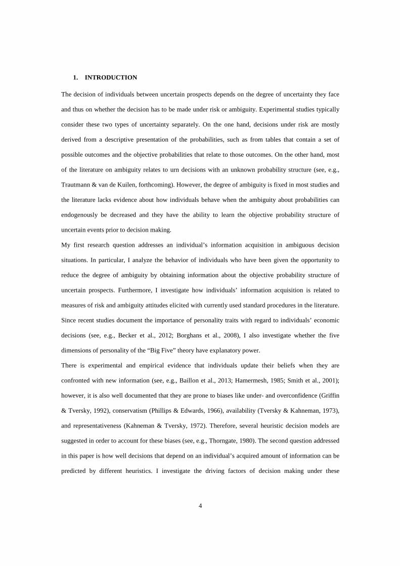
Once a cell is uncovered, the blue or red marble is shown. To prevent any biases related to the ordering of

marbles within an urn, the order is randomized for each subject. The subjects are free to reveal as many

marbles as they want and in any order they wish. There are no financial costs or time limits for revealing

the marbles. In addition, they have the opportunity to count the number of unrevealed red and blue

marbles in each urn automatically by using the corresponding buttons located directly under the

respective urns. The payoffs are displayed above the urns and the subjects are allowed to use an

integrated calculator. Thus, in an extreme case, the experimental design allows the initial situation of total

ambiguity to be turned into a decision under risk by revealing all the marbles. The experimental

framework is distinguished from the descriptive as well as the experience-based format: The probabilities

are not described in tables but rather represented in the form of marbles and the design takes the form of a

draw without replacement.

In order to answer the research questions, the subjects are faced with eight decisions4 in which the urns

are distinguished by three characteristics. In particular, I vary (i) the amount of available information by

varying the number of marbles, (ii) the proportions of red and blue marbles and thus the probability

structure, and (iii) the payoffs by considering the loss and gain domain separately. For each of these three

characteristics, I employ two variations while the other two characteristics are held constant. Thus, the

main part of the experiment uses a 2x2x2 design corresponding to eight treatments, which is explained in

more detail in the following (Table 3 shows an overview).

There are no financial costs or time limits, but the information acquisition process involves effort.

Therefore, the ratio of uncovered marbles might decrease for urns that contain more marbles. In order to

check whether the amount of information, i.e., the total number of marbles, affects the information

acquisition process and decisions, half of the decision tasks deal with 40 marbles and the other half with

80 marbles in each urn. As Table 3 shows, the total number of marbles is always equal for both urns

within a particular decision task. Thus, there are treatments with 80 and 160 cells in total.

4 Probabilities in the decision problems are chosen similar to those in Kahneman and Tversky (1979) and prior studies in psychology (e.g., Hau et al., 2008; Hertwig et al., 2004) that adapt them in order to compare the results. However, they have been modified slightly for the purposes of this study.

12

I consider the gain and the loss domain separately. There are four treatments in which subjects can choose

between two urns, each yielding a negative payoff or nothing. The four treatments that investigate the

subjects’ behavior in the gain domain contain pairs of urns that yield either a positive payoff or nothing.

The subjects face the same decisions for negative and positive payoffs with regard to the probability

structure. As the prospect theory suggests, the decisions are likely to be different depending on whether a

loss or gain is at stake. It is not clear whether the information acquisition is also affected under this

experimental design, however, it seems reasonable that the subjects would show more effort in order to

avoid losses and increase the size of their sample.

Lastly, I vary the proportion of marbles and thus the probabilities of receiving the various payoffs. There

are two different sets of probabilities: The first, referred to as “High,” considers probabilities near to and

equal to one. Urn 2, the one with the smaller gain (EUR 3.00) or smaller loss (EUR -3.00), contains only

blue marbles and thus the respective payoff is always different from zero. As can be seen from Table 3,

the expected value of a random draw from Urn 2 is always EUR 3.00 or EUR -3.00. The other urn in the

“High” probability set, Urn 1, is characterized by higher potential gains or losses of EUR 4.00 or EUR -

4.00, respectively. However, the proportion of red marbles and consequently the probability of receiving

or losing nothing is exactly 15 percent in these urns, irrespective of the total number of marbles.

The expected value of Urn 1 in the gain domain is EUR 3.40 and thus higher than the expected value of

Urn 2. In contrast, Urn 1 has an expected value of EUR -3.40 in the loss domain. This value is below the

expected payoff of Urn 2 (EUR -3.00) and a risk neutral subject should choose Urn 2 under full

information.

To test whether small probabilities are underestimated in this experimental setting, the second set of

probabilities, referred to as “Low,” considers probabilities of 10 and 25 percent for receiving payoffs

different from zero. Similar to the structure of the high probability treatments, the urn with higher gains

or losses (Urn 1) contains more red marbles.

13

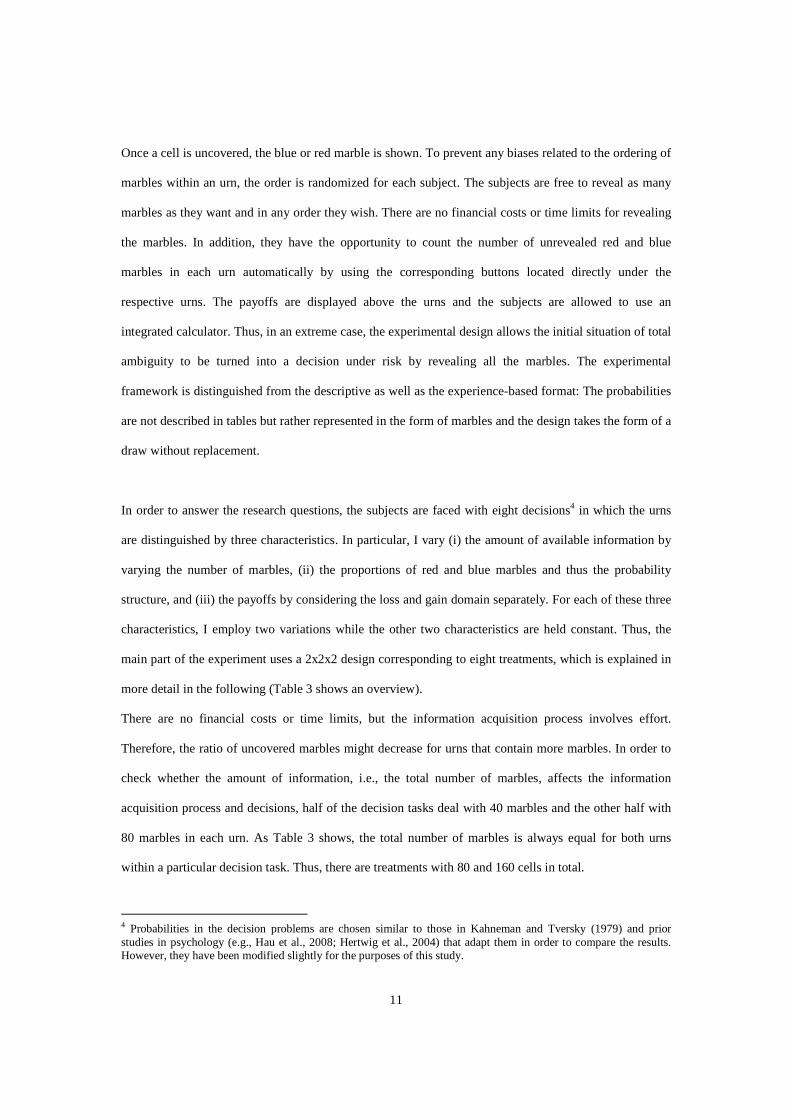
Table 3 Treatments in the urn decision part Urn 1 Urn 2

Treatment Marbles Prob. Payoff Exp.

Payoff Marbles Prob. Payoff

Exp. Payoff

BHP 80 0.85 4.00 3.40 80 1.00 3.00 3.00

BHN 80 0.85 -4.00 -3.40 80 1.00 -3.00 -3.00

BLP 80 0.10 4.00 0.40 80 0.25 3.00 0.75

BLN 80 0.10 -4.00 -0.40 80 0.25 -3.00 -0.75

SHP 40 0.85 4.00 3.40 40 1.00 3.00 3.00

SHN 40 0.85 -4.00 -3.40 40 1.00 -3.00 -3.00

SLP 40 0.10 4.00 0.40 40 0.25 3.00 0.75

SLN 40 0.10 -4.00 -0.40 40 0.25 -3.00 -0.75 Notes: “Marbles” denotes the total number of marbles in each urn. “Prob.” denotes for each urn the probability that a blue marble is randomly drawn. “Payoff” denotes the payoff if a blue marble is drawn. If a red marble is drawn the payoff is always EUR 0.00. The treatments’ labels indicate the variation. “B” and “S” denotes 80 or 40 marbles in each urn, respectively. “H” and “L” denotes high and low probabilities, respectively. “P” and “N” denotes positive and negative payoffs, respectively.

All the subjects face the same decisions, but the order is changed to prevent ordering effects. In

particular, half of the subjects face the problems in a reversed order. Moreover, the location of the urns on

the screen, whether to the left or right, is randomized. The subjects are not informed of the number of

decisions they will face during the sessions. They are only told that they will be confronted with several

choice situations in the first part and that the second part of the experiment will begin after all the

participants have completed the first part. This way, the experimental design avoids time pressure and the

incentive to maximize expected earnings per time.

In order to compare the individual’s behavior under ambiguity and risk, I run an additional session with

full information. The control group is subjected to the identical experiment except for the fact that the

information in the main part, the urn decisions, is not concealed. All the marbles are already visible on the

screen when the subjects enter the stage and there is no ambiguity about the probabilistic structure. Like

in the treatment group, the subjects can count the marbles by using an integrated function.

Measurements of risk and ambiguity aversion

The subjects’ ambiguity attitude is measured with a test based on Halevy (2007). The subjects are again

confronted with two urns containing 10 marbles each. One urn, the risky one, contains exactly five red

14

and five blue marbles. This is known to the subjects. The ambiguous urn also contains red and blue

marbles, but the proportion is unknown. The subjects are asked to predict the color of the marble that is

randomly drawn from each urn by the computer. One urn is randomly chosen to be paid at the end of the

experiment. If the right color of this urn was previously correctly predicted, the subjects receive a payoff

of EUR 6.00, otherwise they get nothing. Prior to the payment and before the subjects know about the

selected urn and the color of the drawn marble, they have the chance to sell each of the two bets to the

computer. In particular, the Becker-DeGroot-Marschak (1964) mechanism is used to elicit the subjects’

reservation prices for both urns. The computer generates a random offer between EUR 0.00 and EUR

6.00. If the subject’s reservation price is higher than the computer’s offer, the marble is randomly drawn

and the subject receives either EUR 0.00 or EUR 6.00. However, if the offer is higher than the reported

reservation price, the bet is sold and the subject receives the amount that is offered by the computer

instead of the reservation price. The dominant strategy for this mechanism is to truthfully report one’s

reservation price. The difference between the subjects’ reported reservation prices for the risky and

ambiguous urn is used as a measure of ambiguity attitude. If the reservation price for the risky urn is

strictly higher than that for the ambiguous urn, the subject is classified as ambiguity-averse. There was a

practice session to ensure that the subjects understood the task (similar to Borghans et al., 2009). Before

the subjects were able to start the actual part of the experiment, they were asked for their reservation price

of a 1-Euro coin. If a subject was not able to give the right answer, the mechanism was explained again.5

I test the subjects’ risk attitude by using a standard lottery choice experiment based on Holt and Laury

(2002), in which the subjects have to choose between two lotteries (X and Y) ten times. Lottery X has a

high payoff of EUR 2.00 and a low payoff of EUR 1.60. Lottery Y has a high payoff of EUR 3.85 and a

low payoff of EUR 0.10. Both lotteries start with the same probabilities of 0.10 for the high payoff. The

probabilities for the high payoffs increase steadily in steps of 0.10. In order to address the fact that the

main task also considers decisions in the loss domain, I also use a Holt-Laury test with the same payoffs

5 This was the case only three times.

15

as losses, which is otherwise identical to the one described above. That means that the subjects can lose

EUR 2.00 or EUR 1.60 by choosing lottery X, and EUR 3.85 or EUR 0.10 by choosing lottery Y.

“Big Five” personality traits

I conducted the test proposed in Gerlitz and Schupp (2005) in order to elicit the subjects’ personality

traits: The Big-Five-Inventory-Shortversion (BFI-S), which consists of a single questionnaire with 15

items.6 The questionnaire contains three items for each of the five personality traits (Neuroticism,

Extraversion, Openness, Agreeableness and Conscientiousness). The statements that consider the

personality traits can be answered by choosing a number from one to seven on a Likert scale, where one

represents total disagreement and seven represents total agreement. Except for Openness, one of the three

items for each personality trait is reverted and presents a negative statement. The number of points from

these items is calculated by subtracting the number of points of the response from eight in order to

account for the reverted character of the statement. Thus, the total number of points for each personality

trait ranges from three in case of total disagreement to 21 in the case of total agreement. The more

response points that a subject has in total, the more pronounced the personality trait. Following Gerlitz

and Schupp (2005), a personality trait is defined as strongly pronounced if a subject assigns a total of

least 15 points to the statements referring to this personality trait.

Finally, the subjects are asked to fill out a questionnaire regarding their personal and educational

background. It also contains a self-assessment question about how they arrive at a decision: “On a scale

from 1 to 5, would you say that you generally decide spontaneously and intuitively or rather that you

consider a decision thoroughly and ponder extensively?”

All parts of the experiment except for the final questionnaire about the personal and educational

background are financially incentivized and paid. From the urn decisions in the main part, one out of

eight decisions is randomly chosen and paid. The payoff ranges from EUR -4.00 to EUR 4.00. A similar

procedure applies for the other parts of the experiment in which one decision is randomly chosen and also

paid. The subjects receive between EUR 0.00 and EUR 6.00 in the second part of the experiment eliciting

6 See Appendix E.

16

the ambiguity attitudes. The payout from the Holt-Laury procedure with positive payoffs ranges from

EUR 0.10 to EUR 3.85 and with negative payoffs from EUR -3.85 to EUR -0.10. In addition, every

subject receives a show-up fee of EUR 4.00 and EUR 4.00 for answering the “Big Five” questionnaire

which ensures that all potential losses during the experiment can be covered.

When the experiment starts, the instructions7 for the first part are handed out and read aloud via an audio

file. The subjects are informed that all of them will start the second part together. They do not receive

information about the other parts and potential payoffs in the following parts. The instructions for the

second part are handed out and read aloud after all the subjects have finished part one. A similar

procedure applies for the following parts of the experiment.

The experiment was programmed with z-tree (Fischbacher, 2007) and conducted at the RUBex

Laboratory of the Ruhr-Universität Bochum, Germany. In total, 59 undergraduate and graduate university

students from different fields of study participated in the experiment. Of this number, 40 percent were

students from the field of management and economics. The average age of the subjects was 24 and 41

percent were males. A total of 46 subjects took part in the treatment session with a covered probability

structure and 13 subjects in the control treatment with full information. The average time of a session was

about 60 minutes and the mean payoff across all sessions was EUR 12.80. The lowest amount paid to a

subject was EUR 2.60 and the highest amount EUR 21.40.8

4. RESULTS

The discussion of the results is ordered in the following way: First, the results for the uncertainty attitudes

and personality traits are presented. Second, an analysis of the subjects’ information acquisition process is

given, followed by an investigation of their decisions.

7 The instructions are available in Appendix F. 8 Includes the show-up fee of EUR 4.00.

17

Uncertainty attitudes and personality traits

I find different patterns for the gain domain (HLP) and the loss domain (HLN) and observe a bimodal

distribution in the case of HLP,9 i.e., the peaks are at measures five and eight. Keeping in mind that a

measure of five in HLP means already switching the first time at the fifth decision to the less risky option

(lottery Y), this finding indicates that a substantial percentage of subjects are less risk averse. In contrast,

switching at the eighth decision corresponds to a relatively high degree of risk aversion. The results show

a unimodal distribution function with a peak at measure six for HLN. I find that 47.45 percent of the

subjects are ambiguity-averse according to the test procedure based on Halevy (2007)10. I do not find a

gender effect for risk aversion or the ambiguity attitude.

Figure 2 gives an overview of the subjects’ personality traits. Neuroticism is the personality trait that is

least pronounced among the subjects, whereas Openness is the most pronounced. The scale’s reliability

with regard to internal consistency, measured by Cronbach’s Alpha, is comparable to the results found by

Gerlitz and Schupp (2005).11

Figure 2 Personality traits pronounced

Notes: Figure 2 shows the percentage in decimal numbers of subjects for whom the respective personality trait is pronounced. “N”, “E”, “O”, “A”, and “C” are binary variables for Neuroticism, Extraversion, Openness, Agreeableness, and Conscientiousness, respectively, and equal to one if the respective personality trait is found to be pronounced; zero otherwise.

9 See Figures 7 and 8 in Appendix A. 10 See Figure 9 in Appendix B. 11 I find the following values for Cronbach’s Alpha: Neuroticism (0.60), Extraversion (0.63), Openness (0.71), Agreeableness (0.50) and Conscientiousness (0.68).

0.36

0.540.59 0.58

0.51

0.00

0.10

0.20

0.30

0.40

0.50

0.60

0.70

N E O A C

18

Table 4 shows the Spearman correlation structure of personality traits and measures of risk aversion and

ambiguity attitude. The mean measure of risk aversion in the gain domain is 6.40. This is above the

corresponding value in the loss domain (6.06), which indicates that, on average, subjects are less risk

averse in the loss domain given the same probability structure. The mean comparison with a two sample

t-test under the assumption of a normal distribution shows no significant difference and the correlation

between HLP and HLN is 0.30 (p = 0.002).

The raw correlation between risk aversion and ambiguity attitude is positive (0.16) and significant (p =

0.002) using the Holt-Laury procedure in the gain domain. The results also show a positive correlation

(0.06) between the ambiguity attitude and risk aversion using HLN. However, this correlation is not

significant (p = 0.601).

Table 4 Spearman correlation structure between personality traits and uncertainty attitudes N E O A C Amb HLP HLN

N 1.00

E -0.31*** 1.00

O 0.10** 0.08* 1.00

A -0.04 0.13*** 0.13*** 1.00

C -0.05 0.27*** 0.28*** 0.39*** 1.00

Amb -0.18*** 0.03 0.26*** 0.21*** -0.01 1.00

HLP -0.11** -0.21*** 0.00 0.21*** -0.04 0.16***

HLN -0.11** -0.28*** -0.01 0.03 -0.06 0.06 0.30***

DT 0.11** -0.04 0.01 0.23*** 0.15*** 0.01 -0.12** -0.07 Notes: “HLP” and “HLN” denotes measures from the Holt and Laury (2002) test considering positive payoffs and negative payoffs, respectively. “Amb” denotes measures from the Halevy (2007) test procedure. “DT” denotes the answers of the self-assessment question considering the decision type. “N”, “E”, “O”, “A”, and “C” are categorical variables for Neuroticism, Extraversion, Openness, Agreeableness, and Conscientiousness. *, **, and *** denotes significance at the 10%, 5%, 1% level, respectively.

Information acquisition

Depending on the treatment, the subjects are able to uncover a total of 80 or 160 cells representing the

marbles in Urn 1 and Urn 2. Figure 3 shows how the total number of marbles uncovered is divided

between Urn 1 and Urn 2, and Figure 4 shows the average of marbles uncovered for each treatment up to

the final decision.

19

Figure 3 Division of total marbles uncovered between Urn 1 and Urn 2

Figure 4 Percentage of total marbles uncovered depending on treatment

Notes: Figure 4 shows the percentage of marbles uncovered for each treatment until subject’s decision is made. “Marbles covered” denotes the percentage of marbles that was left covered.

49.58%50.42% 50.45%49.55% 49.8%50.2%

51.6%48.4% 52.22%47.78% 52.8%47.2%

51.4%48.6% 51.31%48.69%

BHN BHP BLN

BLP SHN SHP

SLN SLP

Urn 1 Urn 2

51.98%48.02%68.57%

31.43%

59.44%40.56%

62.33%

37.67%

86.79%

13.21%

68.97%

31.03%

78.71%

21.29%

74.82%

25.18%

BHN BHP BLN

BLP SHN SHP

SLN SLP

Marbles uncovered Marbles covered

20

As can be seen in Figure 3, the percentage of total marbles uncovered between the urns is almost equal in

all the treatments. I do not observe a significant difference between the urns in terms of information

acquisition within a treatment or between treatments (t-test, p > 0.1). The results indicate that the subjects

reduce ambiguity to the same extent irrespective of whether the payoffs are positive or negative or of the

underlying probability structure.

The average of total marbles uncovered in both urns across all treatments amounts to 79.01 marbles. The

only significant difference that could be observed is between the large and small amounts of available

information. In particular, on average, the subjects uncover 79.34 percent of all the marbles (63.47

marbles) in the treatments with small urns and 59.15 percent (94.64 marbles) in the large urn treatments.

It seems that the more information that is available, the more information that is acquired in absolute

terms, although the number of marbles uncovered decreases for larger urns in relative terms. I do not

observe that the subjects acquire more information in the loss domain in general or find an effect with

regard to different probability structures. Fixed effects panel regressions with the percentage of

uncovered marbles in both urns as dependent variables support these findings as shown in Table 5. The

binary variables for loss and high probability treatments have no significant effect on the amount of

information acquisition in all models. At least the first finding is surprising and in contradiction to the

expectation that subjects show more effort by increasing their sample in order to avoid losses. However,

the binary variable for large urns is significant at the one percent level and confirms that the number of

uncovered marbles decreases with the amount of information available in relative terms. Risk as well as

ambiguity aversion increases the search for information significantly. As it turns out, ambiguity aversion

increases the request for information more than risk aversion. The results show that the interaction

between risk and ambiguity aversion is negative and significant at the one percent level in all models.

This finding indicates that the subjects ask for less information if they are both highly risk-averse and

ambiguity-averse.

21

Table 5 Panel regression models with fixed effects (1) (2) (3) (4) (5) Marbles Beta Beta Beta Beta Beta

Large -0.19*** - -0.20*** - -Loss 0.47 - 0.05 - -HighProb -0.04 - -0.04 - -Risk (HLP/HLN) 0.66*** 0.06*** 0.06*** 0.06*** 0.02Amb 0.29*** 0.30*** 0.30*** 0.27*** 0.35***Risk x Amb -0.02*** -0.03*** -0.03*** -0.02*** -0.02***N - 0.06 0.06 0.06 0.04E - -0.05 -0.05 -0.03 -0.11*O - -0.12*** -0.12*** -0.12** -0.09A - 0.23*** 0.23*** 0.23*** 0.30***C - -0.01 -0.01 0.00 -0.05DT 0.08*** 0.07*** 0.07*** 0.07** 0.09***Female -0.02 -0.06 -0.06 -0.01 -0.08Age 0.01 0.00 0.00 0.01 0.00Stat -0.03 -0.08** -0.08** -0.08 -0.10Order -0.06 -0.05 -0.05 -0.03 -0.10Constant 0.28 0.23 0.38** -0.05 0.98***

Observations 368 368 368 184 184Adj. R� 0.30 0.35 0.31 0.28 0.29

Notes: Table 5 shows the beta coefficients of panel regressions (stage fixed). The dependent variable “Marbles” denotes the percentage of marbles uncovered. “HighProb”, “Loss”, and “Large” are binary variables equal to one if the treatment considers high probabilities, the loss domain, or large urns, respectively; zero otherwise. “Risk” and “Amb” denote risk and ambiguity aversion and “Risk x Amb” denotes the interaction of both variables. “Risk” corresponds to the Holt-Laury measure in the gain domain in models (1)-(4) and in the loss domain in model (5). “N”, “E”, “O”, “A”, and “C” are binary variables for Neuroticism, Extraversion, Openness, Agreeableness, and Conscientiousness, equal to one if the personality trait is pronounced; zero otherwise. “DT” denotes the answers of the self-assessment question considering the decision type. “Female” and “Age” denote gender and age of subjects, respectively. “Stat” is a binary variable equal to one if the subject has taken a statistics course; zero otherwise. “Order” controls for ordering effects. *, **, and *** denote significance at the 10%, 5%, 1% level.

Models (4) and (5) consider the gain and loss domain separately. In model (5), I use the measures from

the Holt-Laury procedure considering negative payoffs (HLN) to control for risk aversion and for the

interaction term between ambiguity attitude and risk aversion. The results change only slightly, however,

the risk measure elicited with the HLN procedure is not significant. Model (4) shows a positive and

significant effect of risk aversion measures on information acquisition by considering only the treatments

with positive payoffs and using HLP to control for risk aversion.

I do not find a gender effect on information acquisition. The variable “DT” denotes the results of the self-

assessment question about the subjects’ decision type (intuitive vs. deliberate) on a scale from one to five,

where “one” means very intuitive and “five” means very deliberate. The coefficient is positive and

22

significant at the one percent level indicating that subjects who consider themselves more deliberate

decision makers request more information. This effect persists when I control for their personality traits

in models (2) to (5).

I find the coefficients of the Openness and Agreeableness variables to be significant at the one percent

level. Subjects, in whom Openness is more pronounced, show less willingness to ask for information but

the amount of acquired information is increased significantly if Agreeableness is more pronounced. In

contrast to my prediction, conscientious subjects do not uncover more marbles. The coefficient is not

significant in models (2) to (5). Thus, I find that two of the “Big Five” personality traits, Agreeableness

and Openness, have explanatory power for an individual’s information acquisition process under

ambiguity beyond the risk and ambiguity measures. Moreover, the explanatory power of those personality

traits is robust against the inclusion of the indicator variables for the treatments (see model (3)).

Decisions

I start with the analyses of the subjects’ decisions with regard to Urn 1 and Urn 2. Figure 5 and Table 6

contain the results for each treatment. The findings document a reflection effect12 by showing that the

subjects’ preferences for the urns are reversed for gains and losses.

In the loss domain, the majority of the subjects prefer Urn 1 with payoffs of EUR -4.00 or EUR 0.00

across all treatments, irrespective of the probability structure and information available, i.e., the size of

the urns. This is true for the treatment and control group, nevertheless the decisions obviously depend on

whether they are made under risk or ambiguity: The subjects in the control group choose Urn 1 more

often in the high probability treatments BHN and SHN, although this urn has a lower expected payoff

(EUR -3.40) than Urn 2 (EUR -3.00). However, I only find a significant difference between treatment and

control group for treatment BHN (Chi2, p = 0.032), not for SHN (Chi2, p = 0.143) as shown in Table 6.

The difference between the treatment and control group is not significant in the low probability

treatments (BLN and SLN). The worst payoff in Urn 1 (EUR -4.00) is lower than in Urn 2 (EUR -3.00),

but Urn 1 has a higher expected payoff (EUR -0.40) than Urn 2 (EUR -0.75). The fact that subjects

12 See Kahneman and Tversky (1979).

23

choose more often Urn 1 indicates that they decide in favor of the urn with higher expected payoff but

also choose the riskier urn in the case of rare events.

With regard to decisions in the gain domain, the subjects show preferences that are reversed. They prefer

Urn 2 with a payoff of EUR 3.00 or EUR 0.00. Thus, in contrast to the decisions in the loss domain, the

subjects avoid gambling for the higher payoff preferring a sure payoff of EUR 3.00. This is particularly

obvious if one compares the decisions under risk in treatments BHN and BHP, which are exactly the

opposite: In treatment BHN, 92.31 percent of the subjects choose Urn 1; and in treatment BHP, 92.31

choose Urn 2. Furthermore, the kind of uncertainty seems to be important for the decisions, although I

only observe a significant difference between the control and treatment group in treatment BHP (Chi2, p =

0.074).

Figure 5 Decisions between Urn 1 and Urn 2 in treatments

60.87%39.13%

92.31%

7.692%32.61%

67.39%

7.692%

92.31%

88.71%

11.29%

84.62%

15.38% 23.33%

76.67%

15.38%

84.62%

54.35%45.65%

76.92%

23.08%41.3%

58.7% 53.85%46.15%

80%

20%

76.92%

23.08% 16.13%

83.87%

23.08%

76.92%

BHN, A BHN, C BHP, A BHP, C

BLN, A BLN, C BLP, A BLP, C

SHN, A SHN, C SHP, A SHP, C

SLN, A SLN, C SLP, A SLP, C

Urn 1 Urn 2

24

Table 6 Decisions between Urn 1 and Urn 2 in treatments

Urn 1

Urn 2 Percentage

choosing Urn 1

Prob. Payoff

Exp. Payoff

Prob. Payoff

Exp. Payoff

A C Diff p

BHP 0.85 4.00 3.40 1.00 3.00 3.00 32.61 7.69 24.92 0.074

BHN 0.85 -4.00 -3.40 1.00 -3.00 -3.00 60.87 92.31 -31.44 0.032

BLP 0.10 4.00 0.40 0.25 3.00 0.75 23.33 15.38 7.95 0.556

BLN 0.10 -4.00 -0.40 0.25 -3.00 -0.75 88.71 84.62 4.09 0.680

SHP 0.85 4.00 3.40 1.00 3.00 3.00 41.30 53.85 -12.55 0.421

SHN 0.85 -4.00 -3.40 1.00 -3.00 -3.00 54.35 76.92 -22.57 0.143

SLP 0.10 4.00 0.40 0.25 3.00 0.75 16.13 23.08 -6.95 0.547

SLN 0.10 -4.00 -0.40 0.25 -3.00 -0.75 80.00 76.92 3.08 0.820

Notes: “A” and “C” denotes the ambiguity or control treatment, respectively. “Prob.” denotes for each urn the objective probability that a blue marble is randomly drawn. “Payoff” denotes the payoff in Euro if a blue marble is drawn; if a red marble is drawn the payoff is always EUR 0.00. The treatments’ labels indicate the variation. “B” and “S” denotes 80 or 40 marbles in each urn, respectively. “H” and “L” denotes high and low probabilities, respectively. “P” and “N” denotes positive and negative payoffs, respectively. “p” denotes p-values (Chi2).

I investigate the subjects’ decisions in more detail by taking their individual knowledge about the

probabilistic structure into account. Therefore, I consider five heuristics that are reasonable for the

prediction of subjects’ decisions. They are introduced in Section 2 and their implications for this

particular experiment are briefly explained below. Application of the Maximax heuristic means that a

subject chooses the urn with a payoff of EUR 4.00 in the gain domain. The high payoff in the loss domain

is EUR 0.00 for both urns and the subjects need to apply the second decision rule of this heuristic, which

assumes that they decide in favor of the urn with the highest sample probability for the high payoff (EUR

0.00). If a subject applies the Minimax heuristic, the urn with a payoff of EUR -3.00 is chosen in the loss

domain because this decision minimizes the potential loss. In the gain domain, the urn with the highest

sample probability for the smallest loss is selected, which is identical for both urns and equal to EUR

0.00. Adapting the theoretical proceedings of the Most Likely and Least Likely heuristics to this study’s

framework implies the following behavioral strategies: In order to choose the urn for which the high

payoff occurs most frequently in their sample (Most Likely) the subjects would have to count the blue

marbles in their sample in the gain domain and the red ones in the loss domain. Note that a red marble in

the loss domain means that the payoff of EUR 0.00 occurs while a blue marble means that a loss of EUR

25

-4.00 or EUR -3.00 occurs. If subjects choose the urn for which the worst payoff is observed least

frequently (Least Likely), they have to count the red marbles in the gain domain which corresponds to a

payoff of EUR 0.00. In the loss domain, they have to count the blue marbles in their sample which

corresponds to a payoff of EUR -4.00 (Urn1) and EUR -3.00 (Urn 2). Note that the Most Likely and

Least Likely heuristics predict the same decisions for each of the eight decision problems based on the

objective probability structure; this means that Most Likely and Least Likely predict the same decisions

under risk. However, the predictions are distinct for the decisions under ambiguity and depend on the

individual sample.

Figure 6 shows the performance of each heuristic in terms of correct predictions. It is important to keep in

mind that the heuristics overlap under the study’s experimental design - or are even equal as in the case of

the Least Likely and Most Likely heuristics in the control group.

I find that the Least Likely and Most Likely heuristics are the best predictors of the subjects’ decisions

under risk (79 precent). Under ambiguity and based on the individual amount of information, Most Likely

performs best in correctly predicting the subjects’ decisions (72 percent) and turns out to be significantly

better than Least Likely (z-test, p < 0.05), which correctly predicts 65 percent of all the decisions. The

two heuristics that primarily focus on outcomes, Minimax and Maximax, perform worse than the dual

heuristics Most Likely and Least Likely, irrespective of whether the decision is one under risk or

ambiguity (z-test, p < 0.05). Moreover, the predictions based on the heuristic that assumes subjects

choose in favor of the urn with the higher expected payoff (EP) are significantly worse than those based

on the Most Likely and Least Likely heuristics in the control and the treatment group (z-test, p < 0.05).

Figure 6 also shows the percentage of subjects who decide against the prediction of the expected payoff

heuristic (EP) but according to the Minimax (“DiffMin”) or Maximax (“DiffMax”) heuristic. I find that

the Maximax heuristic is applied more frequently if the decision is not in line with the expected payoff

heuristic (z-test, p < 0.1). This indicates that more subjects decide in favor of maximizing their potential

payoff even if the decision is against the urn with the highest expected payoff.

26

Figure 6 Performance of heuristics

Notes: Figure 6 shows the percentage in decimal numbers of correct predictions. “Risk” indicates the control group and “Ambiguity” the treatment group. “”DiffMax” and “DiffMin” indicate the percentage of those subjects who decide not in line with the EP heuristic but instead according to Minimax and Maximax, respectively.

To complete the picture and in order to analyze how personality traits and uncertainty attitudes influence

the subjects’ decisions, I run logit estimations with a binary variable of whether the urn is chosen in line

with the respective heuristic (see Table 7 for the results).

Neither risk aversion nor ambiguity attitude are found to have a significant influence on whether the

decision is made by applying the Minimax, Maximax, Most Likely, or Least Likely heuristic. In contrast,

model (1) reveals a positive effect of these measures on decisions based on the expected payoff (EP)

under ambiguity. Model (2) also shows that risk aversion has a positive effect on this decision rule under

risk.

Minimax is applied significantly more often in high probability treatments and in the loss domain, as can

be seen from the estimations in models (6) and (7). Moreover, conscientious subjects seem to decide

more often in order to minimize their potential loss (Minimax) and less often in order to maximize gains

(Maximax). Deliberate thinker and females decide less frequently according to the Minimax heuristic.

Considering the dual heuristics, I find that the subjects decide significantly less often according to the

Most Likely or Least Likely heuristic under ambiguity in high probability treatments (models (3) and

0.52

0.79 0.79

0.21

0.56

0.04

0.21

0.61

0.72

0.65

0.22

0.46

0.080.13

0.00

0.10

0.20

0.30

0.40

0.50

0.60

0.70

0.80

0.90

EP ML LL Min Max DiffMin DiffMax

Risk Ambiguity

27

(4)). Moreover, they decide less often in line with the Least Likely heuristic in the loss domain, which

indicates that subjects do not try to minimize their potential loss (model (4)). Under risk, model (5)

reveals that subjects apply the Most Likely and Least Likely heuristics more often if they are confronted

with large amounts of information. With regard to the subjects’ personality traits, the results show that

neurotic subjects decide significantly less often in line with the predictions of the Least Likely and Most

Likely heuristics under ambiguity. Subjects for whom Conscientiousness is more pronounced are also

less likely to decide according to these heuristics. I observe no effect of personality traits on whether the

decision is made according to Most Likely and Least Likely under risk. I find that the decisions under

ambiguity according to the Least Likely and Most Likely heuristics are more often made by females.

Furthermore, subjects who consider themselves reasonable thinkers decide in line with the Least Likely

and Most Likely heuristics under ambiguity considerably more frequently.

Models (8) and (9) show that subjects for whom Conscientiousness is more pronounced decide in line

with the Minimax heuristics more frequently and less often in line with the Maximax heuristic if they do

not rely on the expected payoff heuristic (EP). If subjects make their decision under risk rather than

ambiguity, they are more likely to decide in order to maximize their potential payoff (Maximax), as can

be seen from model (9). I find that the Minimax heuristic correctly predicts fewer decisions of reasonable

thinkers when they decide against the urn with the higher expected payoff.

28

Table 7 Logit estimations of urn decisions

(1) (2) (3) (4) (5) (6) (7) (8) (9)EP EP ML LL ML/LL Min Max DiffMin DiffMax

Marbels 0.00* - 0.02 0.01** - - - - -HighProb -1.66*** -1.73*** -1.25*** -0.82*** -0.69 1.14*** -0.18 - -Loss -0.33 -1.13** 0.04 -0.80*** 0.69 0.67*** 1.80*** - -Large 0.25 -0.80* -0.28 0.10 1.30** -0.39 0.20 - -Risk 0.14** 1.85** 0.05 0.03 -2.77 0.01 -0.02 -0.05 -0.12*Amb 0.51* - 0.28 0.21 - -0.34 -0.29 -0.57 -0.07N -0.36 -0.91 -1.01*** -0.87** 14.08 0.61* 0.00 0.16 -0.28E 0.66** 3.58 0.46 0.50* -10.72 -0.04 0.17 -0.17 -0.21O -0.20 1.59 -0.61* -0.61* 1.73 0.43* 0.28 0.93** 0.34A -0.68** -0.80 0.85*** 1.06*** 11.15 -0.94*** 0.23 -0.45 0.60*C -0.12 -2.87 -1.61*** -1.57*** 6.65 1.19*** -0.62** 1.30** -0.66*DT 0.10 3.28** 0.48*** 0.53*** 9.28 -0.36* 0.03 -0.53** -0.05Female 0.37 0.84 1.70*** 1.30*** 6.50 -0.90** 0.25 -0.50 0.18Age 0.04 0.34* 0.03 0.04 -2.00 -0.01 0.02 -0.06 -0.04Stat -0.23 0.16 0.13 0.04 -10.01 0.17 0.35 0.78 0.24Order 0.48* -0.51 -0.16 0.01 24.01 -0.04 -0.01 -0.03 -0.16

Control - - - - - -0.39 0.56* -0.91 0.78**Constant -1.59 -26.98 -2.01 -1.83 9.23 -0.89 -1.79 -0.43 -0.08

Observations 368 104 368 368 104 472 472 472 472

Pseudo R� 0.16 0.17 0.23 0.17 0.26 0.13 0.15 0.11 0.03Notes: Table 7 shows the results of different logit estimations of urn choices. “DiffMin” and “DiffMax” indicate the decisions that are not in line with EP but according to Minimax and Maximax, respectively. “Marbles” denotes the number of marbles uncovered. “HighProb”, “Loss”, and “Large” are binary variables equal to one if the treatment considers high probabilities, the loss domain, or large urns, respectively; zero otherwise. “Risk” and “Amb” denote risk and ambiguity aversion, respectively. “N”, “E”, “O”, “A”, and “C” are binary variables for Neuroticism, Extraversion, Openness, Agreeableness, and Conscientiousness, respectively, equal to one if the personality trait is pronounced; zero otherwise. “DT” denotes the answers of the self-assessment question considering the decision type. “Female” and “Age” denote gender and age of subjects, respectively. “Stat” is a binary variable equal to one if the subject has token a statistics course; zero otherwise. “Order” controls for ordering effects. “Control” denotes the control group. *, **, and *** denote significance at the 10%, 5%, 1% level. For “Risk” I used measures from HLP; using HLN did not change any results.

29

5. DISCUSSION

Information acquisition and decisions

I find that ambiguity is almost never completely reduced, which implies that the utility from reducing

ambiguity is described by a concave function. The marginal utility from reducing ambiguity

decreases with the amount of information and tends to zero. It is notable that the average number of

marbles uncovered in the large urn treatments (94.64 marbles) exceeds the total number of marbles

presented in the small urn treatments (80 marbles). This is remarkable since this finding excludes

cognitive costs as an explanation for the fact that ambiguity is not completely reduced in the majority

of decision tasks. This reasoning would imply that subjects forgo obtaining more information because

they cannot process it; however, this is contradicted by the results. Moreover, the experiment

excludes any time restrictions or financial costs. The issue of effort seems to be the only source of

costs that might prevent them from acquiring all the information. The tradeoff between showing more

effort and leaving some degree of ambiguity is almost always in favor of some residual ambiguity,

which the subjects seem to feel comfortable with. Thus, there is an individual threshold of tolerated

ambiguity. The results indicate that this threshold depend neither on whether the decision is made in

the gain or loss domain nor on the probabilistic structure. Furthermore, consistent with my prediction,

the individual sample size is much higher than in experimental studies considering learning from

experience.

Neither the variables for risk aversion nor ambiguity attitude seem to influence whether the decision

is made by applying several heuristics or not - except for the one considering the expected payoff.

With respect to a subject’s ambiguity attitude, it can be argued that this characteristic should only

influence the individual sample size, which is indeed confirmed by the analysis, and not the decision

itself. However, this reasoning does not seem applicable in the case of risk aversion. In contrast, I

observe a positive effect of both risk and ambiguity aversion measures on decisions that are in line

with the expected payoff heuristic. I conclude that the influence of uncertainty measures is limited to

this heuristic, regardless of whether the decision is made under ambiguity or risk. If the subjects

30

know the objective probability structure, they obviously rely on the Most Likely and Least Likely

heuristics more often in the case of large urns.

I find different results for particular personality traits with regard to their explanatory power for both

individuals’ information acquisition and their final decisions according to all heuristics. I find a

negative influence of the Openness variable on sample size, which does not seem intuitive at first

glance. However, Openness captures “individual differences in the tendency to be open to new

aesthetic, cultural, and intellectual experiences” according to the definition13 rather than curiosity.

Although a certain degree of curiosity could be seen as a kind of prerequisite for new experiences, the

other component of the definition seems to outweigh this. Surprisingly, the Conscientiousness

variable turns out to have no significant influence on sample size, which is in contradiction to my

prediction. As Table 4 shows, the Conscientiousness variable is not correlated with risk aversion or

ambiguity attitude measures. The results show that Conscientiousness influences the decision itself

but not the amount of information a subject acquires prior to a decision. As predicted, I find the

explanatory power of personality traits to be different for information acquisition and decisions.

Moreover, the explanatory power is different for decisions under risk and those under ambiguity.

An individual’s decision type (intuitive vs. deliberate) influences both information acquisition and

decisions. Deliberate thinkers request significantly more information prior to their final decision.

With regard to the decisions themselves, I find different effects for risk and ambiguity. Under

ambiguity, deliberate thinkers choose more often according to the Least Likely and Most Likely

heuristic; however, I do not find an effect for whether the decision is made in favor of the highest

expected payoff (EP). Under risk, the opposite is the case: I observe that subjects in the control group

decide in favor of the higher expected payoff (EP) more often, but I find no effect as to whether the

decision is made in line with the Least Likely or Most Likely heuristic. A possible explanation of this

finding might be that, under risk, subjects know the objective probability structure and can better

estimate the expected payoff. However, based on the fact that subjects do not count the number of

marbles or use the calculator I rule out the explanation that they really calculate and decide according

to the expected payoff.

13 See Table 1.

31

I find that the predictions of the decisions of females with the Minimax heuristic are considerably

worse (p < 0.05). Since this implies that females decide less frequently in order to limit their potential

loss, this finding is not in line with the general result that females are more risk-averse. Moreover, I

observe no gender effect on risk aversion elicited with the Holt-Laury test.

Summing up, I do not find that standard measures of risk and ambiguity aversion explain the

decisions according to four out of five heuristics included in the study. Fully consistent with my

expectation, I find that individuals’ personality traits have explanatory power for decisions and

information acquisition beyond the measures of uncertainty. In addition, the experiment provides

evidence that an individual’s decision type influence the acquisition of information and decision. In

contradiction to the majority opinion, I do not observe clear evidence of a gender effect with regard

to the risk attitude. This is true considering the elicited measures using the standard procedures and

the behavior observed in the main decision task with regard to the information acquisition and the

decision itself according to the predictions of five different heuristics included in the study.

Presentation format and reflection effect

Despite the fact that the experiment provides a design in which the degree of ambiguity is

endogenous, it turns out that the presentation format affects the subjects’ decisions. As previously

described, the study finds evidence of a reflection effect. Some of the study’s decision problems are

similar to prior studies, in which the problems from Kahneman and Tversky (1979) are adapted.

Hertwig et al. (2004) investigate individual decisions under risk with a focus on rare events and

learning from experience. Their experiment contains some of the same decisions used in Baron and

Erev (2003), who investigate feedback-based individual decisions (see Table 8 for an overview). The

treatments BHP, SHP, BHN, and SHN are almost identical to those in prior studies. The treatments

BLP SLP, BLN, and SLN are similar and also shown in Table 8; however, the probabilities are

slightly different thereby resulting in different expected payoffs. Therefore, drawing conclusions

from a comparison of these results must be done with care.

32

The control or descriptive groups in prior studies received the information displayed in a typical table

containing the outcomes and probabilities. In this study’s experimental setting, the marbles in the

urns are presented instead. Table 8 contains a comparison of the results. The comparison shows that

under this different presentation format the amount of information, i.e., the number of marbles I

present to the subjects, impacts the decision under risk with a known objective probability structure

as well as under ambiguity. It is noteworthy that the subjects in the control treatment are also able to

let the computer count the number of marbles. If they had done this, the framework would have been

nearly identical to the treatments in prior studies since the subjects would have had the objectively

presented information at hand. Interestingly, this is not done by the subjects.14 One conceivable

reason for this behavior might be that they feel comfortable with the presentation of probabilities and

do not see added value in counting the number of marbles.

14 It was done only 17 times across all treatments and subjects.

33

Table 8 Comparison of results with prior studies

Option 1 Option 2 Choice 1

Prob. Outc.a Exp Prob. Outc.a Exp C/Des A

BHP 0.85 4.00 3.40 1.00 3.00 3.00 7.69 32.61

SHP 0.85 4.00 3.40 1.00 3.00 3.00 53.85 41.30 Kahneman & Tversky

0.80 4,000 3,200

1.00 3,000 3,000

20 -

Barron & Erev 0.80 4.00 3.20 1.00 3.00 3.00 55 -

Hertwig et al. 0.80 4.00 3.20 1.00 3.00 3.00 36 -

BHN 0.85 -4.00 -3.40 1.00 -3.00 -3.00 92.31 60.87

SHN 0.85 -4.00 -3.40 1.00 -3.00 -3.00 76.92 54.35 Kahneman & Tversky

0.80 -

4,000 -

3,200

1.00 -

3,000 -

3,000

92 -

Barron & Erev 0.80 -4.00 -3.20 1.00 -3.00 -3.00 70 -

Hertwig et al. 0.80 -4.00 -3.20 1.00 -3.00 -3.00 72 -

BLP 0.10 4.00 0.40 0.25 3.00 0.75 15.38 23.33

SLP 0.10 4.00 0.40 0.25 3.00 0.75 23.08 16.13 Kahneman & Tversky

0.20 4,000 800

0.25 3,000 750

65 -

Barron & Erev 0.20 4.00 0.80 0.25 3.00 0.75 81 -

Hertwig et al. 0.20 4.00 0.80 0.25 3.00 0.75 64 -

BLN 0.10 -4.00 -0.40 0.25 -3.00 -0.75 84.62 88.71

SLN 0.10 -4.00 -0.40 0.25 -3.00 -0.75 76.92 80.00 Kahneman & Tversky

0.20 -

4,000 -800

0.25

-3,000

-750

42 -

Notes: “C” denotes the control group which corresponds to the descriptive group in Hertwig et al. (2004), Baron and Erev (2003), and Kahneman and Tversky (1979). “A” denotes the treatment group. “Outc.” denotes outcome. a Outcome corresponds to a payment in Euro in this study. In Kahneman and Tversky (1979) outcome denotes Israeli pounds, but the experiment was in questionnaire form with hypothetical questions. In Baron and Erev (2003) and Hertig et al. (2004) outcome denotes points, whereas one point corresponds to a payment of 0.01 Shekel or 0.02 US Dollar, respectively.

As can be seen in Table 8, I do not find the reflection effect as observed under the descriptive

conditions in prior studies. In the low probability treatments, the reflection effect is observable in the

opposite direction. While Kahneman and Tversky (1979) and other studies find that the majority of

subjects, i.e., more than 50 percent, choose Option 1 for the positive payoffs and Option 2 for the

negative ones, this study finds the subjects behavior to be the exact opposite. This is true irrespective

of the size of the urn presented to the subjects. As already noted, the results should be interpreted

with care because the probabilities are not exactly the same and consequently the expected payoff

differs. The observed behavior would be in line with prior studies if it is assumed that the subjects

decide according to the expected payoff. However, the subjects do not know the expected payoff or

34

the exact numbers of colored marbles because they do not count them15. Thus, it seems unlikely that

the differences in probabilities and expected payoffs are the only drivers for the observed effects.

In addition, Table 8 shows the result of this study with regard to the treatment group which mirrors

my findings for the control group and shows the reflection effect for treatments in the gain domain

even more clearly. Keeping in mind that the subjects almost never uncover all the marbles and thus

do not get to learn the objective probability structure, it appears even more unlikely that the

differences in probabilities between this and prior studies cause the inversion of the reflection.

The findings indicate that the presentation format impacts individual decisions, at least for low

probabilities. Furthermore, the subjects seem to feel comfortable with the presentation format in this

study since they do not switch to a descriptive format by counting the marbles. Assuming that the

standard descriptive format produces less biased decisions, the results of this study imply the

following: First, that irrespective of whether the decision is made under risk or ambiguity, the

subjects decisions are biased, and second that the subjects are not aware of this bias because they do

not switch the format. While many decisions are certainly made under conditions similar to a

descriptive presentation format this does not apply for all decisions, especially those outside the

laboratory. Decisions under presentation formats similar to the one chosen in this study might

produce very different decision behavior.

6. CONCLUSION

This paper analyzes individual information acquisition and decisions under risk and ambiguity. The

experimental design allows the subjects to endogenously and individually determine the degree of

ambiguity prior to making a decision without financial costs or time constraints.

I observe that both risk aversion and ambiguity aversion are positively related to the amount of

information that subjects acquire. The interaction coefficient between the risk aversion and ambiguity

aversion variables is negative, which indicates that subjects make decisions based on less information

if they are both risk and ambiguity-averse. I do not observe a gender effect on the sample size, but the

results indicate that Openness and Agreeableness have explanatory power for the subjects’

information acquisition beyond the measures for risk and ambiguity. Individuals for whom

15 I cannot rule out the possibility that they count the marbles manually; however, this seems very unlikely since they could count them by simply clicking on a button, which would have been documented by the program.

35

Agreeableness is more pronounced reduce the degree of ambiguity more than others and individuals

for whom Openness is more pronounced acquire less information. In contrast to my prediction,

conscientious subjects do not acquire more information.

With regard to the decisions, I find that the standard measures of risk and ambiguity aversion do not

explain the decisions for four of the five heuristics incorporated in this study. I conclude that their

explanatory power in a non-standard experimental situation is limited. I do not observe clear evidence

of a gender effect with regard to the risk attitude. This is true considering the elicited measures using

the standard procedures and the behavior observed in the main decision task with regard to the

information acquisition and the decision itself according to the predictions of five different heuristics

included in the study.

In contrast, it is the individual’s personality traits, gender and decision type that turn out to have

explanatory power for the decision. Decisions are best predicted by the dual heuristics Least Likely

and Most Likely. The measure of Conscientiousness affects the subject’s decision: The results

indicate that conscientious subjects aim to minimize their potential loss.

The study documents a reflection effect, but finds that the effect is reversed for low probabilities

compared to studies using a descriptive format for presenting the probability structure. This is the

case for decisions under ambiguity as well as those under risk. Thus, the presentation format seems to

cause a different decision behavior, at least for low probabilities. While many decisions are certainly

made under conditions captured by the standard descriptive presentation format this does not apply

for all decisions, especially those outside the laboratory. Decisions under presentation formats similar

to the one chosen in this study might produce very different decision behavior.

36

References Baillon, A., Bleichrodt, H., Keskin, U., L’Haridon, O., & Li, C. (2013). Learning under ambiguity:

An experiment using initial public offerings on a stock market. Working Paper, No. 201331. Center for Research in Economics and Management (CREM), University of Rennes 1, University of Caen and CNRS.

Barron, G., & Erev, I. (2003). Small feedback-based decisions and their limited correspondence to description-based decisions. Journal of Behavioral Decision Making, 16 (3), 215-233. Becker, A., Deckers, T., Dohmen, T., Falk, A., & Kosse, F. (2012). The relationship between

economic preferences and psychological personality measures. The Annual Review of Economics, 4, 453-478.

Becker, G., DeGroot, M., & Marschak, J. (1964). Measuring utility by a single-response sequential method. Behavioural Science 9 (3), 226-32. Borghans, L., Golsteyn, B. H. H., Heckman, J. J., & Huub, M. (2009). Gender differences in risk

aversion and ambiguity aversion. Journal of the European Economic Association, 7 (2-3), 649-658.

Borghans L., Duckworth, A. L., Heckman, J. J., & ter Weel, B. (2008). The economics and

psychology of personality traits. The Journal of Human Resources, 43 (4), 972-1059. Cowan, N. (2001). The magical number 4 in short-term memory: A reconsideration of mental storage

capacity. Behavioral and Brain Sciences, 24, 87-114. Fischbacher, U. (2007). z-Tree: Zurich Toolbox for Ready-made Economic Experiments. Experimental Economics,10 (2), 171-178. Gerlitz, J.-Y., & Schupp, J. (2005). Zur Erhebung der Big-Five-basierten Persönlichkeitsmerkmale im SOEP. Research Notes, 4, DIW Berlin. Gigerenzer, G., P., Todd, M., & the ABC Research Group. (1999). Simple heuristics that make us smart. New York. New York University Press. Gigerenzer, G., & Hoffrage, U. (1995). How to improve Bayesian reasoning without instruction: Frequency formats. Psychological Review, 102 (4), 684-704. Griffin, D., A. Tversky. (1992). The weighing of evidence and the determinants of confidence. Cognitive Psychology, 24, 411-435. Halevy, Y. (2007). Ellsberg revisited: An experimental study. Econometrica, 75 (2), 503-536. Hamermesh, D. S. (1985). Expectations, life expectancy, and economic behavior. The Quarterly

Journal of Economics, 100 (2), 389-408. Hau, R., Pleskac, T. J., & Hertwig, R. (2010). Decisions from experience and statistical probabilities:

Why they trigger different choices than a priori probabilities. Journal of Behavioral Decision Making, 23 (1), 48-68.

Hau, R., Pleskac, T. J., Kiefer, J., & Hertwig, R. (2008). The description-experience gap in risky choice: The influence of sample size and experienced probabilities. Journal of Behavioral Decision Making, 21 (5), 493-518. Hertwig, R. (2012). The psychology and rationality of decisions from experience. Synthese, 187 (1),

269-292.

37

Hertwig, R., Barron, G., Weber, E. U., & Erev, I. (2004). Decisions from experience and the effect of rare events in risky choice. Psychological Science, 15 (8), 534-539. Holt, C., & Laury, S. K. (2002). Risk aversion and incentive effects. American Economic Review,

92 (5), 1644-1655. Kahneman, D., & Tversky, A. (1979). Prospect theory: An analysis of decision under risk. Econometrica, 47 (2), 263-291. Kahneman, D., & Tversky, A. (1974). Judgment under uncertainty: Heuristics and biases. Science, 185 (4157), 1124-1131. Kahneman, D. (1973). Attention and Effort. Englewood Cliffs, NJ, Prentice-Hall. Kahneman, D., & Tversky, A. (1972). Subjective probability: A judgment of representativeness. Cognitive Psychology, 3(3), 430-454. Kareev, Y., Lieberman, I., & Lev, M. (1997). Through a narrow window: Sample size and the

perception of correlation. Journal of Experimental Psychology: General, 126 (3), 278-287. Phillips, L. D., & Edwards, W. (1966). Conservatism in a simple probability inference task. Journal of Experimental Psychology, 72 (3), 346-354. Rakow, T. & Newell, B. R. (2010). Degrees of uncertainty: An overview and framework for research on experience-based choice. Journal of Behavioral Decision Making, 23 (1), 1-14. Smith, V. K., Taylor Jr, D. H., and Sloan, F. A. (2001). Longevity expectations and death: Can people predict their own demise? American Economic Review, 91 (4), 1126-1134. Thorngate, W. (1980). Efficient decision heuristics. Behavioral Science, 25 (3), 219-225. Trautmann, S., & van de Kuilen, G. (forthcominig). Ambiguity attitude. Blackwell Handbook of Judgment and Decision Making. Tversky, A., & Kahneman, D. (1981). The framing of decisions and the psychology of choice. Science, 211 (4481), 453-458. Tversky, A., & Kahneman, D. (1992). Advances in prospect theory: Cumulative representation of

uncertainty. Journal of Risk and Uncertainty, 5 (4), 297-323. Ungemach, C., Chater, N., & Stewart, N. (2009). Are probabilities overweighted or underweighted

when rare outcomes are experienced (rarely)? Psychological Science, 20 (4), 473-479.

38

Appendix A. Results from Holt-Laury procedure

Figure 7 Results from Holt-Laury test procedure with positive payoffs

Figure 8 Results from Holt-Laury test procedure with negative payoffs

Notes: Figure 7 shows the percentage of subjects for the measures of the Holt-Laury test with positive payoffs. Figure 8 shows the percentage of subjects for the measures of the Holt-Laury test with negative payoffs.

1.695

3.39

1.695

6.78

22.03

11.86

15.25

25.42

6.78

5.085

05

10

15

20

25

Pe

rce

nt

0 2 4 6 8 101 3 5 7 9

HLP

1.6953.39

8.475

11.86

38.98

23.73

8.475

3.39

01

02

03

04

0P

erc

en

t

0 2 4 6 8 101 3 5 7 9

HLN

39

Appendix B. Results from the Halevy procedure

Figure 9 Distribution of subjects’ ambiguity aversion

Notes: Figure 9 shows the percentage of subjects for the reservation prices according to the Halevy test.

5.085

10.17

37.29

13.56

25.42

1.695

6.78

01

02

03

04

0P

erc

en

t

-1 0 1 20.5-0.5-1,5 1.5Ambiguity attitude

40

Appendix C. Decision mode

Figure 10 Distribution of subjects’ primary decision mode

Notes: Figure 10 shows for each measure of decision mode the percentage of subjects according to the self-assessment question. “1” denotes “very intuitive” and “5” denotes “very deliberate”.

3.39

23.7325.42

44.07

3.39

01

02

03

04

0P

erc

en

t

0 1 2 3 4 5

Decision mode

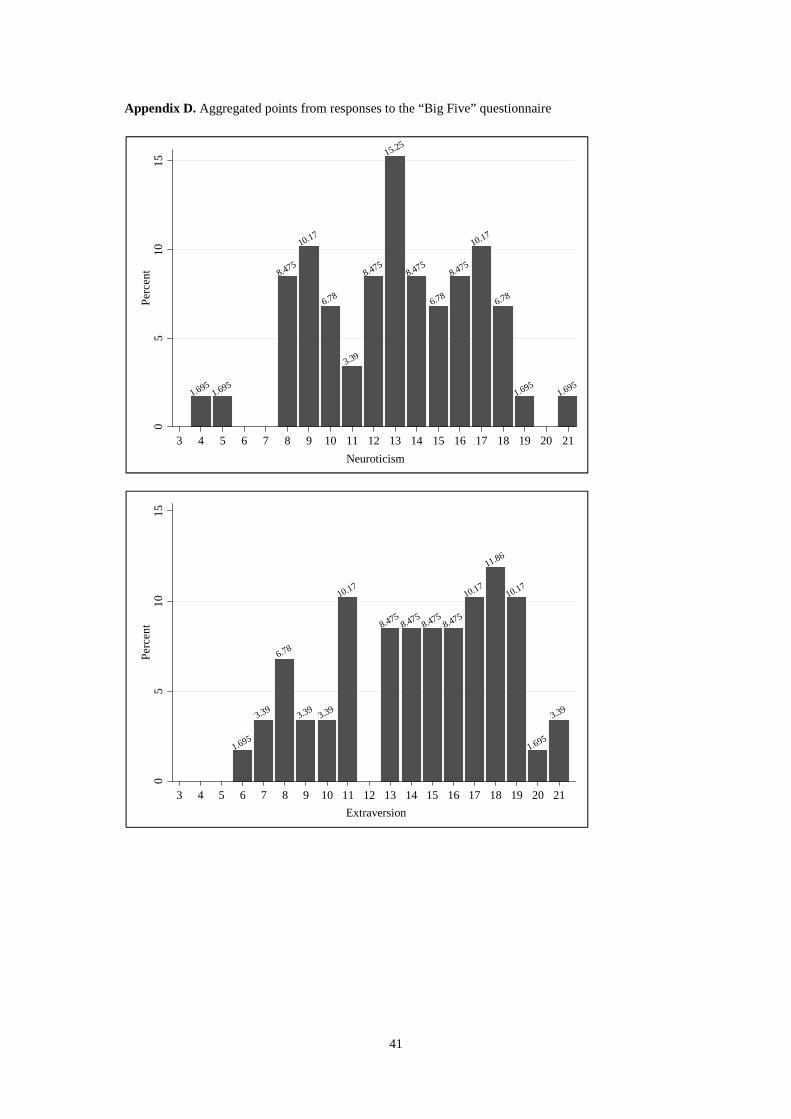
41

Appendix D. Aggregated points from responses to the “Big Five” questionnaire

1.6951.695

8.475

10.17

6.78

3.39

8.475

15.25

8.475

6.78

8.475

10.17

6.78

1.6951.695

05

10

15

Pe

rce

nt

5 10 15 203 4 6 7 8 9 11 12 13 14 16 17 18 19 21

Neuroticism

1.695

3.39

6.78

3.393.39

10.17

8.4758.475

8.4758.475

10.17

11.86

10.17

1.695

3.39

05

10

15

Pe

rce

nt

5 10 15 203 4 6 7 8 9 11 12 13 14 16 17 18 19 21

Extraversion

42

1.6951.695

1.695

3.39

8.475

6.78

10.17

6.78

13.56

10.17

18.64

6.78

3.39

1.695

5.085

05

10

15

20

Pe

rce

nt

3 4 5 6 7 8 9 10 1211 13 14 15 16 17 18 19 20 21Openness

5.0855.085

6.78

3.39

10.17

11.86

10.17

11.86

13.56

11.86

5.085

3.39

1.695

05

10

15

Pe

rce

nt

5 10 15 203 4 6 7 8 9 11 12 13 14 16 17 18 19 21

Agreeableness

43

Notes: The figures show for each personality trait the percentage of subjects who are assigned the respective number of total points. The total number of points ranges from 3 in case of total disagreement among all three items presented in the questionnaire to 21 in case of total agreement. The more points a subject responds in sum, the more the personality trait is pronounced.

1.695

3.39

5.085

10.17

6.78

8.475

13.56

6.78

11.86

8.475

13.56

5.085

1.695

3.39

05

10

15

Pe

rce

nt

5 10 15 203 4 6 7 8 9 11 12 13 14 16 17 18 19 21

Conscientiousness

44

Appendix E. “Big Five” inventory

Big-Five-Inventory-Shortversion (BFI-S) following Gerlitz and Schupp (2005)

The questionnaire contains a 15-item Likert scale considering the five personality traits Neuroticism, Extraversion, Openness, Agreeableness, and Conscientiousness. Answering is possible on a scale from “1” to “7”, where “1” means total disagreement and “7” total agreement. I see myself as someone who…

gets nervous easily ⃝ ⃝ ⃝ ⃝ ⃝ ⃝ ⃝

N

worries a lot ⃝ ⃝ ⃝ ⃝ ⃝ ⃝ ⃝

N

is relaxed, handles stress well ⃝ ⃝ ⃝ ⃝ ⃝ ⃝ ⃝

N-

is communicative ⃝ ⃝ ⃝ ⃝ ⃝ ⃝ ⃝

E

is outgoing, sociable ⃝ ⃝ ⃝ ⃝ ⃝ ⃝ ⃝

E

is reserved, quiet ⃝ ⃝ ⃝ ⃝ ⃝ ⃝ ⃝

E-

has an active imagination ⃝ ⃝ ⃝ ⃝ ⃝ ⃝ ⃝

O

is original, comes up with new ideas ⃝ ⃝ ⃝ ⃝ ⃝ ⃝ ⃝

O

Values artistic, aesthetic experiences ⃝ ⃝ ⃝ ⃝ ⃝ ⃝ ⃝

O

is considerate and kind to almost everyone ⃝ ⃝ ⃝ ⃝ ⃝ ⃝ ⃝

A

has a forgiving nature ⃝ ⃝ ⃝ ⃝ ⃝ ⃝ ⃝

A

is sometimes rude to others ⃝ ⃝ ⃝ ⃝ ⃝ ⃝ ⃝

A-

does things efficiently ⃝ ⃝ ⃝ ⃝ ⃝ ⃝ ⃝

C

does a thorough job ⃝ ⃝ ⃝ ⃝ ⃝ ⃝ ⃝

C

tends to be lazy ⃝ ⃝ ⃝ ⃝ ⃝ ⃝ ⃝

C-

Notes: “N” denotes Neuroticism, “E” denotes Extraversion, “O” denotes Openness, “A” denotes Agreeableness, and “C” denotes Conscientiousness. Statements were presented in a random order. The right column was not presented and assigns the corresponding personality trait to each statement. A minus indicates that the item contains a reverted statement. The questionnaire does not include a reverted statement for Openness.

total agreement

total disagreement

45

Appendix F. Instructions

Instructions Welcome to the experiment. From now on, please do not speak to the other participants of the experiment and use only those functions on the computer that are required for the experiment. The purpose of this experiment is to examine different forms of decision-making behaviour; hence there are no right or wrong answers. You can earn money in this experiment. The amount paid depends on your own decisions and chance according to the rules on the following pages. The data from the experiment are made anonymous and cannot be associated with the participants. Both during and after the experiment, neither the other participants nor the conductors of the experiment will come to know which decisions you made and how much you earned. You receive an amount of 4.00 Euro for showing up. This amount will be added to the payoff obtained in the experiment. Procedure The experiment consists of several parts that are relevant to the payment. These parts will be explained on the following pages. After the experiments, please answer a short questionnaire containing questions about yourself. Payout Your total payoff at the end of the experiment is the sum of your profits and losses from all parts of the experiment plus the 4.00 Euro for showing up. All in all, you can make no loss. After you have filled in the short questionnaire, you will be called out one by one. Please bring the small card with your number and the completed and signed receipt to the payout. The payment will be conducted anonymously and in private.

46

Part 1

Task In Part 1 of the experiment you have to choose between two urns, out of which the computer will draw a marble. The urns contain red and blue marbles. You will see the urns depicted on your screen. The boxes or buttons are equivalent to one marble. The buttons conceal the colour of the marbles, which are randomly distributed by the computer. If you click the button to learn more about the composition of the urn, the button will vanish and the colour of the marble underneath will become visible. Below each urn, there is a button saying “count marbles”. Click this button in order to make the computer count the number of revealed red and blue marbles. If you reveal more marbles after the counting, you will have to click the button again in order to learn about the current number of revealed red and blue marbles. You can take as long as you want for your decision. You can reveal as many marbles as you wish by clicking on them. However, if you do not want to, you do not have to reveal any marbles at all. The payoffs of the urns can be positive or negative, i.e. there are also decisions that result in a loss. The possible payoffs are explained above each urn.

You decide from which urn the marble will be drawn!

Example

Payout At the end of the experiment, one of the pairs of urns will be chosen by the computer; all of the pairs are chosen with the same probability. The computer will randomly draw a marble from the urn you have chosen before from this pair, according to the relation of the probabilities of the marbles in that urn. You will then receive the gain or loss from this drawing as a payoff in Euro.

Payoffs, if you draw a blue marble, you receive 4 Euro, if you draw a red marble you receive 0 Euro

Marbles in the urn, concealed by buttons

Number of the revealed red and blue marbles in the urn

Button to count the marbles

47

Part 2 Task In the second part of the experiment, there are two different urns. Each of these urns contains 10 marbles, some of which are red and some of which are blue. Your first task is to predict the colour of the marble the computer will draw for each urn. The proportion of the marbles’ colours varies between the two urns. You win if the colour you predicted is drawn. But you also have the possibility to do without the drawing from the urns and receive a safe amount by selling the drawing to the computer. In order to do this, you have to tell the lowest amount between 0.00 Euro and 6.00 Euro that you would accept for selling the bet.

• The computer generates a random offer. If the offer is below the price you mentioned, it was not possible to sell the drawing, hence the drawing takes place and determines your payoff.

• If the offer is above the price you mentioned, you successfully sold the drawing to the

computer and receive the offer from the computer. No marbles will be drawn from the urns. Payout One of the two urns will be chosen for the payout. The computer randomly generates an offer between 0.00 Euro and 6.00 Euro. If this is above the price you named, you receive the offer from the computer. If the computer’s offer is below the price you named, the drawn colour will determine your payoff. A marble will be drawn randomly from the urn.

• If you predicted the colour correctly, you receive 6.00 Euro.

• If you did not predict the colour correctly, you receive 0.00 Euro.

48

Part 3 & Part 4 Task In the parts 3 and 4 you have to decide between two lotteries (X and Y) ten times. In each lottery, you can win one of two amounts of money (Part 3) or lose one of two amounts of money (Part 4). The procedure is the same in both parts. The probabilities of winning or losing the prizes are different for each decision. Example Lottery X I choose X I choose Y Lottery Y 3/10, 2.00 € 7/10, 1.60 € € € 3/10, 3.85 € 7/10, 0.10 € … … € € … …

Each lottery has two possible results, which have certain possibilities. The result is determined by drawing a random number. In the example above you can win a price of 2.00 Euro with a probability of 3/10 and a price of 1.60 Euro with a probability of 7/10 in lottery X. In lottery Y you can win a price of 3.85 Euro with a probability of 3/10 and a price of 0.10 Euro with a probability of 7/10. Please make your choice for all the ten lotteries. After that you can confirm the computer screen with the “O.K.” button. Payout At the end of the experiment, one of the ten lottery pairs from part 4 and one of the pairs from part 5 will be chosen. Each of the pairs has the same probability of 1/10. The lottery (X or Y) of those chosen pairs that you have decided for before will be played. As a payoff from part 4 and part 5 you receive the gain or loss that was randomly chosen in the chosen lotteries.