Embed Size (px)
Citation preview

Repeat-Punctured Turbo Trellis-
Coded Modulation
Rinel Bhownath
University Of Kwa-ZuluNatal Durban, South Africa
July 2010
Submitted in fulfilment of the requirements for the degree of Master of Science in
Engineering, in the Department of Electronic Engineering.

i
Statement of Originality
All material contained in this thesis consist of the original work of the author unless otherwise stated and has not been previously submitted for a degree in this or any other university.

ii
As the candidate’s supervisor, I have approved this dissertation for submission.
Name : Prof. Hongjun Xu
Signed: ____________________________
Date: ____________________________

iii
Acknowledgements
I would like to thank my Supervisor Prof H. Xu for his support, motivation and guidance
throughout my MSc. Degree. I would like to thank Telkom for the opportunity to complete
my masters. I would also like to thank my family, my brothers and especially my mum, for
tolerating me for so many years. Finally I would like to dedicate my thesis to my late father
DAN.
iv
Abstract
Ever since the proposal of turbo code in 1993, there has been extensive research carried out
to improve both the performance and spectrum efficiency. One of the methods used to
improve the spectrum efficiency was to combine turbo code with a trellis-coded modulation
scheme, called turbo trellis-coded modulation (TTCM). The scheme is used in various
applications such as deep-space communication, wireless communication and other fields.
It is a well established fact that an increase in an interleaver size of a TTCM system results in
an improved performance in the bit error rate (BER). In this thesis repeat-punctured turbo
trellis-coded modulation (RPTTCM) is proposed. In RPTTCM, the effect of repeat-puncture
is investigated on a TTCM system, repetition of the information bits increases the interleaver
size, followed by an appropriate puncturing scheme to maintain the respective code rate. The
TTCM and RPTTCM systems are simulated in an Additive White Gaussian Noise (AWGN)
channel. To understand how the RPTTCM scheme will perform in a wireless channel, the
Rayleigh flat fading channel (with channel state information known at the receiver) will be
used. The BER performance bound for the TTCM scheme is derived for AWGN and
Rayleigh flat fading channels. Thereafter repeat-punctured is introduced into the TTCM
system. The BER performance bound is then extended to include repeat-puncturing. The
performances of the TTCM and RPTTCM systems are then compared. It was found that the
RPTTCM system performed better at high signal-to-noise ratio (SNR) in both AWGN and
Rayleigh flat fading channels. The RPTTCM scheme achieved a coding gain of
approximately 0.87 dB at a BER of ���� for an AWGN channel and 1.9 dB at a BER of ���� for a Rayleigh flat fading channel, for an information size of N=800.

v
Table of contents
Abstract ..................................................................................................................................... iv
List of Figures ........................................................................................................................ viii
List of Symbols ......................................................................................................................... xi
List of Tables ........................................................................................................................... xii
List of Acronyms ................................................................................................................... xiii
Chapter 1: Introduction .......................................................................................................... 1
1.1 Motivation of Research .................................................................................................... 1
1.2 Outline of Dissertation ..................................................................................................... 3
Chapter 2 : Basic of Communication ......................................................................................... 4
2.1 Digital Communication System ....................................................................................... 4
2.2 Noise................................................................................................................................. 5
2.3 Convolutional Code.......................................................................................................... 5
Chapter 3: Turbo Trellis-Coded Modulation, Repeat-Punctured Turbo Trellis Coded Modulation ................................................................................................................................. 9
3.1 Turbo Code ....................................................................................................................... 9
3.1.1 Turbo Encoder ........................................................................................................... 9
3.1.2 Turbo Decoder ......................................................................................................... 11
3.1.2.1 Iterative MAP Decoder .................................................................................. 11
3.1.2.2 Iterative MAP Algorithm............................................................................... 12
3.2 Trellis Coded Modulation .............................................................................................. 23
3.2.1 Encoder .................................................................................................................... 23
3.2.2 Decoder .................................................................................................................... 25
vi
Chapter 4: Performance Analysis of a Turbo Trellis-Coded Modulation and Repeat-Punctured Turbo Trellis-Coded Modulation Scheme ............................................................................... 27
4.1 Derivation of the Performance Bound for a TTCM scheme in an AWGN channel ...... 27
4.1.1 Expected Number of Codewords ............................................................................. 28
4.1.2 Determining the Square Euclidean Distance ........................................................... 31
4.1.3 Results ..................................................................................................................... 33
4.2 Derivation of the Performance Bound for RPTTCM in an AWGN channel ................. 35
4.3 Derivation of the Performance Bound in a Rayleigh Flat Fading channel .................... 38
4.3.1 Performance Bound of TTCM scheme .................................................................... 38
4.3.2 Performance Bound of RPTTCM scheme ............................................................... 39
4.4 Comparison of the Performance Bound for the TTCM and RPTTCM Schemes…….. 41
Chapter 5: Turbo Trellis-Coded Modulation and Repeat-Punctured Turbo Trellis Coded Modulation ............................................................................................................................... 45
5.1 Turbo Trellis-Coded Modulation ................................................................................... 45
5.1.1 Encoder Structure .................................................................................................... 45
5.1.2 Iterative Decoder ..................................................................................................... 48
5.1.2.1 Log Likelihood Ratio for an AWGN Channel .............................................. 49
5.1.2.2 Log Likelihood Ratio for a Rayleigh Fading Channel .................................. 50
5.1.3 Simulation Results ................................................................................................... 51
5.2. Repeat-Punctured Turbo Trellis-Coded Modulation ..................................................... 53
5.2.1. Encoding Structure ................................................................................................. 53
5.2.2 Modified Iterative Decoder ..................................................................................... 54
5.2.3 Simulation Results ................................................................................................... 56
vii
5.3 Comparison between Turbo Trellis-Coded Modulation and Repeat-Punctured Turbo
Trellis-Coded Modulation Simulation Results ..................................................................... 57
Chapter 6: Conclusion and Future Research ............................................................................ 63
6.1 Conclusion ...................................................................................................................... 63
6.2 Future Research .............................................................................................................. 64
APPENDIX .............................................................................................................................. 65
A: Input-Output Weighted Enumerating Function (IOWEF) .............................................. 65
References ................................................................................................................................ 68
viii
List of Figures
Fig. 2.1 Basic block diagram of a digital communication system.
Fig. 2.2 (a) A ���� convolutional encoder, (b) state diagram of the ���� convolutional
encoder.
Fig. 2.3 (a) A ������ RSC encoder, (b) state diagram of a ������ encoder.
Fig. 2.4 A ������ RSC encoder with trellis termination.
Fig. 3.1 Basic structure of a turbo encoder.
Fig. 3.2 Illustration of a random interleaver.
Fig. 3.3 Structure of an iterative MAP decoder.
Fig. 3.4. Graphical representation of the reverse probability function.
Fig. 3.5 Graphical representation of the forward probability function.
Fig. 3.6. A rate of 2/3 TCM encoder.
Fig. 3.7 Signal mapping for a rate of 2/3 TCM scheme using 8PSK modulation.
Fig. 3.8 Modified trellis diagram taking into account an uncoded bit.
Fig. 4.1 Rate 1/2 TTCM Scheme.
Fig. 4.2 16-QAM gray mapping for the information and parity bits.
Fig. 4.3 Performance bound for a TTCM scheme in an AWGN channel for different number
of error terms � ��. Fig. 4.4 Performance bound of the TTCM scheme in an AWGN channel using information
weight of � � �� � � ��and � � �� Fig. 4.5 Simulation results and performance bound of a TTCM scheme for N=200 in an
AWGN channel.
ix
Fig. 4.6 RPTTCM encoder scheme.
Fig. 4.7 Simulation results and BER performance bound of a RPTTCM scheme for N=200 in
an AWGN channel.
Fig. 4.8 Simulation results and BER performance bound of a TTCM scheme for N=200 in a
Rayleigh flat fading channel.
Fig. 4.9 Simulation results and BER performance bound of a RPTTCM (L=2) scheme for
N=200 in a Rayleigh flat fading channel.
Fig. 4.10 Performance bound and simulation result for a RPTTCM and TTCM scheme for an
information size N=200 in an AWGN channel.
Fig. 4.11 Expected number of codewords for a RPTTCM (L= 2, 3) and a TTCM scheme for
an information length of N = 200.
Fig. 4.12 Performance bound and simulation result for a RPTTCM and TTCM scheme for an
information size N=200 in a Rayleigh flat fading channel.
Fig. 5.1 Encoding structure for a TTCM Scheme.
Fig. 5.2 Odd-even puncturing pattern for the TTCM Scheme.
Fig. 5.3 16-QAM mapping of the information and parity bits.
Fig. 5.4 Iterative decoding structure for a TTCM scheme.
Fig. 5.5 Simulation of TTCM scheme in an AWGN channel for an information size of N=200
and N=800.
Fig. 5.6 Simulation of TTCM scheme in a Rayleigh flat fading channel with the CSI known
at the receiver for an information size of N=800 and N=200.
Fig. 5.7 Encoding structure of a RTTCM scheme.
Fig. 5.8 Puncture scheme for the RPTTCM Scheme (L=2).
Fig. 5.9 Iterative decoding structure for a TTCM scheme.
x
Fig. 5.10 Simulation of RPTTCM (L=2) scheme in an AWGN channel for an information
size of N=200 and N=800.
Fig. 5.11 Simulation of RPTTCM (L=2) scheme in a Rayleigh flat fading channel with the
CSI known at the receiver for an information size of N=800 and N=200.
Fig. 5.12 Simulation results for the RPTTCM (L=2) and the TTCM scheme in an AWGN
channel for an information size of�� � ���.
Fig. 5.13 Simulation results for the RPTTCM (L=2) and the TTCM scheme in an AWGN
channel for an information size of � � ���.
Fig. 5.14 Simulation results for the RPTTCM (L=2) and the TTCM scheme in a Rayleigh Flat
fading channel with the CSI known at the receiver for an information size of � � ���.
Fig. 5.15 Simulation results for the RPTTCM (L=2) and the TTCM scheme in a Rayleigh flat
fading channel with the CSI known at the receiver for an information size of � � ���.
Fig. A1 (a) A ���� convolutional encoder, (b) state diagram of the ���� convolutional.
encoder.
Fig. A2 Modified trellis diagram taking into account the punctured states.
xi
List of Symbols
�� Information bit sequence.
��� Interleavered information bit sequence.
� �� Parity sequence of encoder i.
�� The one sided power spectrum density of an AWGN channel.
��� Transmitted sequence.
��� Received sequence.
! Variance of an AWGN channel.
"� State of a RSC code.
#� �$�� $ State transition probability of the MAP algorithm.
%��$ Forward state probability of the MAP algorithm.
&��$ Reverse state probability of the MAP algorithm.
� ��� Log likelihood ratio using the MAP algorithm for the ��' decoder.
� (��� Extrinsic information for the ��' decoder.
���� A-priori probability.
% Fading coefficient.
)* Bit error rate probability.
) ���+ Number of different interleavers.
, ��� -. Number of codewords for encoder i.
/�+ Number of error sequences.
0+�1! Square Euclidean distance due to an error sequence.
2013 Total number of received codewords resulting in an error distance 01!� 41�5 Error distance profile.
4+ Total error distance due to an error sequence.

xii
List of Tables
Table 5.1 Summary of the simulation results of a TTCM and a RPTTCM scheme in a AWGN
channel.
Table 5.2 Summary of the simulation results of a TTCM and a RPTTCM scheme in a
Rayleigh flat fading channel.
xiii
List of Acronyms
AWGN Additive White Gaussian Noise TCC Turbo Coded Cooperation SCTC Superorthogonal Convolutional Turbo Code RPSCTC Repeat-Punctured Superorthogonal Convolutional Turbo Code RPCTC Repeat-Punctured Superorthogonal Convolutional Turbo Code BER Bit Error Rate SNR Signal-to-Noise-Ratio TC Turbo Code TCM Trellis-Coded Modulation TTCM Turbo Trellis-Coded Modulation RPTTCM Repeat-Punctured Turbo Trellis-Coded Modulation RSC Recursive Systematic Convolutional PCCC Parallel Concatenated Convolutional Code MAP Maximum A-Posteriori Probability VA Viterbi Algorithm SOVA Soft Output Viterbi Algorithm LLR Log Likelihood Ratio
QAM Quadrant Amplitude Modulation
1
Chapter 1: Introduction
1.1 Motivation of Research
Ever since the introduction of the mathematical study of communication by Shannon in 1973
[1], where he defined the maximum theoretical capacity of a communication system. This has
lead to a spark in the field of error correcting codes. There have been many error correcting
codes developed since then. However no such scheme has achieved near Shannon limits as
that of turbo code, developed by C. Berrou [2], in 1993. The encoding structure is simple,
consisting of parallel concatenated RSC encoders connected via an interleaver. Ever since the
publication of turbo code, there has been extensive research carried out to improve the
performance. The various areas of turbo code that effect its performance are;
I. RSC encoder
♦ The type of generator polynomial used by the encoder effects the
performance [3].
♦ Increasing the constrain length (memory size of the RSC encoder) results
in an increase in performance [3].
♦ Increasing the number of parallel concatenated RSC encoders has a slight
increase in performance [4].
II. Decoder
♦ The type of iterative decoder used has an effect on the performance. The
iterative maximum a-priori probability (MAP) decoder has a better
performance than the iterative soft-output Viterbi algorithm (SOVA)
decoder [3]. However the iterative MAP algorithm is fairly complicated
and computational long. Therefore the iterative Log-MAP decoder was
developed to reduce computational difficulty as well as the complexity.
The iterative Log-MAP decoder has a slight degradation in performance
compared to the iterative MAP algorithm but still has a better performance
compared to the iterative SOVA.
♦ Increasing the number of iteration of the decoding algorithm increases the
performance of the system irrespective of the type of decoding algorithm
2
used. However, after a certain number of iteration, the increase in
performance is eligible [5-7].
III. Puncturing
♦ Puncturing (deletion of certain bits) is used to increase the code rate. This
comes with a drop in performance. However there exists an optimal
puncturing pattern that reduces the degradation in performance [5, 7-9].
IV. Interleaver
♦ There are various types of interleavers developed for turbo code: S-
random, code matching and random (uniform) interleaver just to name a
few. The code-matching interleaver results in the best performance,
followed by the S-random interleaver [3]. The increase in performance
comes with an increase in complexity.
♦ The size of the interleaver used has a large effect on the performance of
turbo code (interleaver gain) [10-13], irrespective of the type of interleaver
used.
Examining the effects of various aspects have on the performance of the turbo code, the
inteleaver size has the best potential in increasing the performance. A method to exploit the
performance gain due to the interleaver size was developed in [14] using repeat-puncturing.
The repetition of information bits allows the use of a larger interleave size than that of the
information size. Thereafter the encoded bits are punctured to maintain the code rate. The
repeat-punctured turbo code (RPTC) scheme showed a coding gain of approximately 1.5 dB
at a bit error rate (BER) of ���6 compared to traditional turbo code. Repeat-puncturing was
extended to turbo code cooperation (TCC) system in [15] and superorthogonal convolutional
turbo code (SCTC) in [16]. The repeat-punctured turbo code cooperation (RPTCC) system
achieved a coding gain of approximately 1.8 dB at a BER of ���7 while the repeat-punctured
superorthogonal convolutional turbo code (RPSCTC) system achieved a coding gain of
approximately 1.4 dB at a BER of ����. Both the RPSCTC and the RPTCC systems were
then extended to a dual repeat-punctured system. The dual repeat-punctured SCTC achieved
a coding gain of approximately 0.25 dB at a BER of ���6 compared to the RPSCTC system
while the dual repeat-punctured TCC system achieved a coding gain of approximately 1.5 dB
at a BER of ���7 compared with the RPTCC system.
3
Turbo code has exceptional performance at low SNR, however it does not exploit the
availability of bandwidth. Trellis-Code Modulation (TCM) developed by Ungerboeck,
consisted of a convolutional code that maps �8 information bits to a �8�.-Mary modulation
scheme, using the set partition method. The performance of TCM scheme is not as great as
that of turbo code, but has high bandwidth efficiency. It was only natural to combine the
performance of turbo code with the bandwidth efficiency of TCM. The scheme developed is
called Turbo Trellis-Coded Modulation (TTCM) [12, 17-18]. Since RPTC has better BER
performance compared to conventional TC, it is natural to combine RPTC with TTCM,
called repeat-punctured trellis-coded modulation (RPTTCM). In this thesis we investigate the
BER performance of RPTTCM. An encoding method along with a modified iterative
decoding algorithm is discussed. The performance bound of a TTCM scheme is explained
and then extended to a RPTTCM scheme.
1.2 Outline of Dissertation
An introduction to the basics of digital communication is presented in chapter 2. A basic
overview of an overall digital communication system is discussed along with the types of
noise that effects the system. Thereafter the fundamentals of turbo codes and trellis-coded
modulation are discussed in Chapter 3. The various elements that make up a turbo coded
system, interleaver, puncturing and encoders are discussed. The decoding structure of the
turbo code is derived and discussed. The basic encoding and decoding structure of a trellis-
coded modulation scheme is discussed. In Chapter 4 the derivation of the BER performance
bound for the TTCM scheme is explain for a AWGN channel. Thereafter the derivation is
extended to a Rayleigh flat fading channel. The performance bound of the TTCM scheme is
then modified to take into account repeat-puncturing. The BER performance bound of the
RPTTCM scheme is derived for both noise channels. In Chapter 5 we discussed the turbo
trellis-coded modulation (TTCM) encoder and decoder structure. The TTCM scheme is
simulated in both AWGN and Rayleigh flat fading channel. The modification needed at the
TTCM encoder and decoder to take into account repeat-puncturing is discussed. The
simulation results of the RPTTCM scheme is compared with that of the TTCM scheme.
Finally Chapter 6 contains the conclusion as well as details for future research.
4
Chapter 2 : Basic of Communication
2.1 Digital Communication System
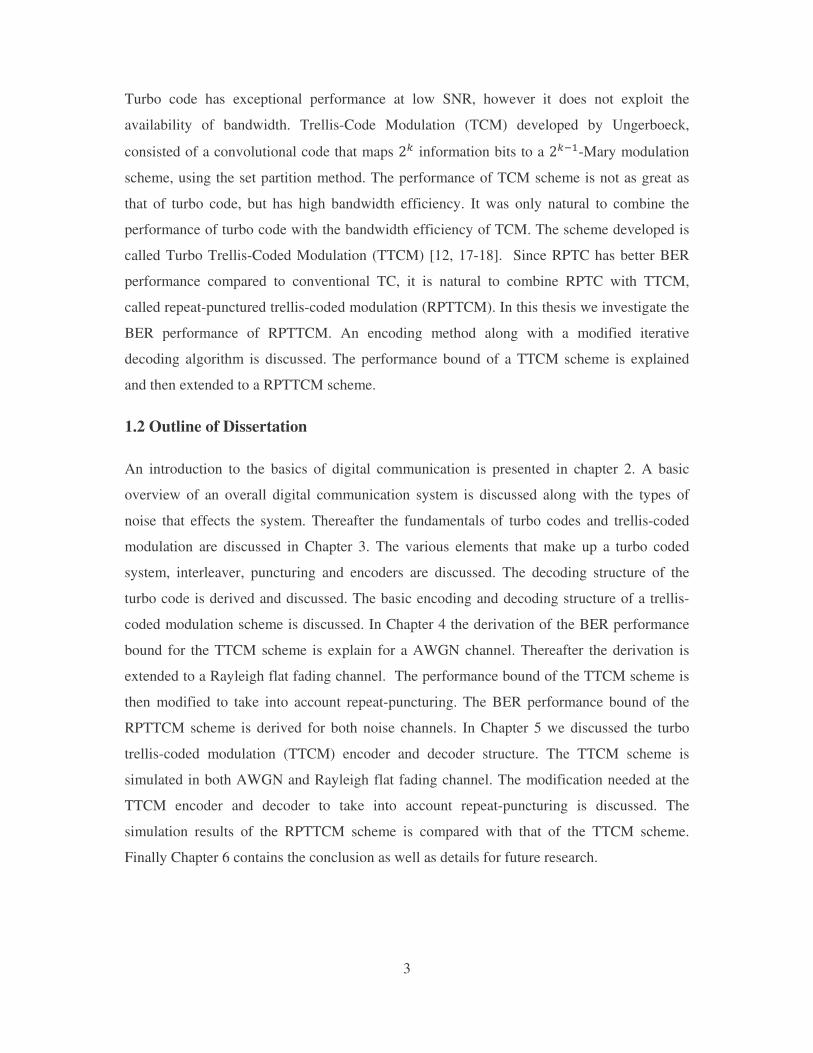
The basic structure of any digital communication system is shown in Fig. 2.1. The system can
be broken into three distinct sections: a transmitter, a communication channel and a receiver
section.
Fig. 2.1 Basic block diagram of a digital communication system.
The transmitter is made up of the following subsections: information source, source coding,
channel coding and modulation. Information source represents the raw data that is required to
be transmitted. Depending on the type of data being transmitted, there may exist certain
redundancy in the information source. If we transmit the information source with the
redundancy, we reduce the efficiency of the system. Therefore the information source is sent
to the source encoder, in order to remove redundancy. At this stage the data is in general not
suitable for transmitting in a noisy channel. The channel encoder is used to add redundancy,
i.e., for every k information bits an extra n redundant bits are added to the transmitted
sequence. Note that the source encoder removes redundancy since it reduces the efficiency of
the system. The added redundancy from the channel encoder is used to correct errors due to a
noisy channel. Finally we need to transmit the digitally encoded information over the
channel. The modulator maps the digital information into various parts of a sinusoidal wave.
This is achieved by varying either the frequency, amplitude or the phase of the sinusoid.
The transmitted sequence corrupted by noise introduced by the communication channel is
received at the receiver section. The function of the receiver is to minimise the effect of noise
and recover the transmitted sequence. The first step of the receiver is to demodulate the
received sequence by extracting the relative information from the sinusoid. The received
sequence can be in the form of a hard or soft decision, depending on the decoder algorithm
used at the channel decoder. Thereafter the channel decoder is used to correct any error
5
introduced by the channel. The received sequence is then decoded based on the method used
at the encoder section.
2.2 Noise
For any electrical system there contains an unwanted electrical disturbance. Like all systems,
noise places a huge problem in the telecommunication field, since transmitted messages are
altered, resulting in an incorrect message received. This unwanted signal has given birth to a
research field in error correcting code for telecommunication systems. One of the most
important channel models used for digital communication system is the Additive-White-
Gaussian-Noise (AWGN) channel. The noise is added to a transmitted signal as follows
9 � : ; � (2.1)
where : represents the transmitted signal, 9 denotes the received signal corrupted by noise, �
is a zero-mean AWGN variable with variance ! � �� �< � and �� is the one sided power
spectrum density of the noise.
However, an AWGN channel does not model a wireless channel since transmitted signals
suffer from degradation due to scattering, reflection and diffraction. We will be focusing on a
Rayleigh flat fading channel, which is used to model a non-line-of-sight communication link.
The term flat fading means all frequency component of a transmitted signal experience the
same magnitude of fading. Rayleigh flat fading is added to the transmitted sequence as
follows:
9 � %: ; � (2.2)
where % is the fading coefficient.
2.3 Convolutional Code
A simple example of a block diagram of a convolutional code (trellis code) is shown in Fig.
2.2. (a). It consists of two shift registers (memory blocks) D1 and D2, as well as Exclusive
OR (XOR) operators arranged in varies configurations. Convolutional codes can be thought
of as a finite state machine, where the output is determined by the present state of the shift
6
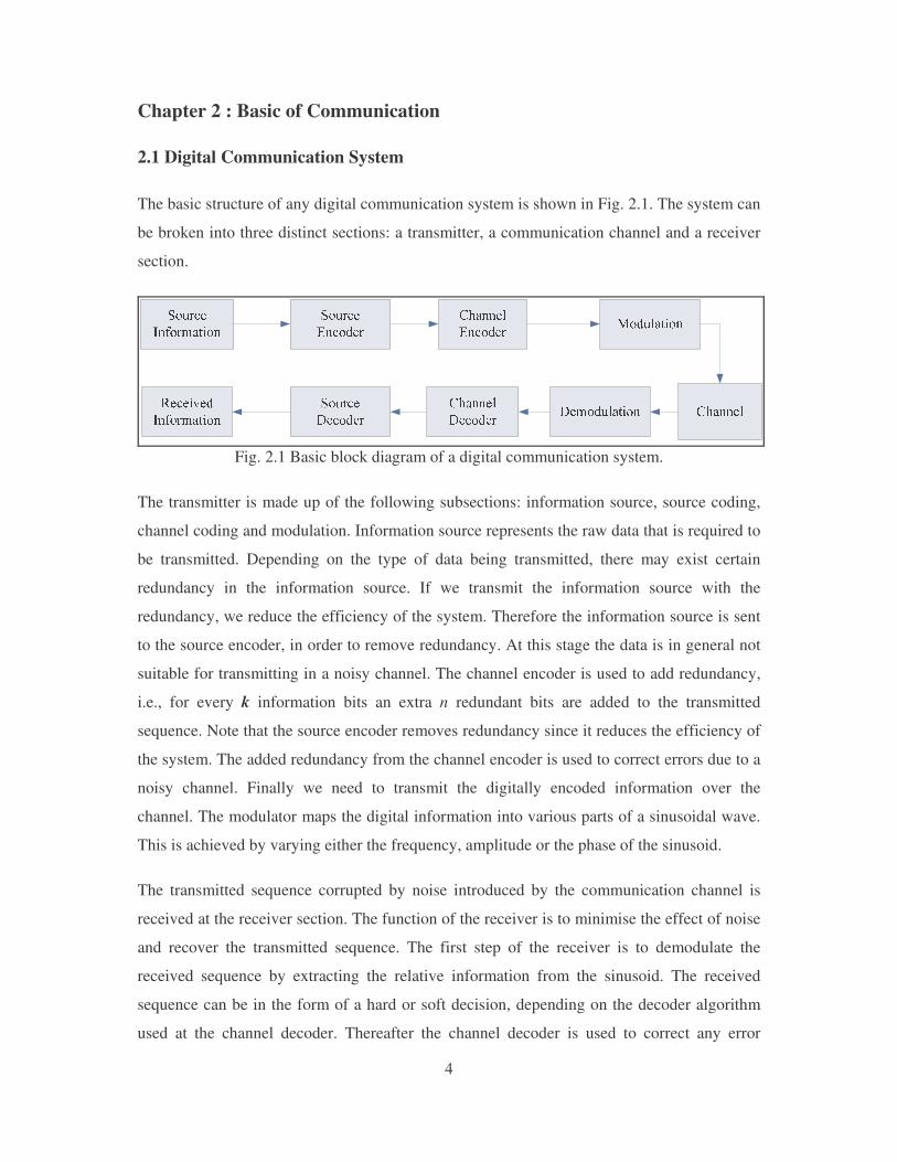
registers as well as the input bits. The convolutional code shown in Fig. 2.2.(a) consists of a
generator polynomial of G([1 1 1], [1 0 1] ). We will be using the notation ��� � which is in
the octal form. Fig. 2.2.(b) shows the corresponding state diagram of the convolutional code.
Fig. 2.2 (a) A ���� convolutional encoder, (b) state diagram of the ���� convolutional
encoder.
The information bit �� at time , enters the encoder, producing two parity bits �.�� and �!��. For a ���� the parity bits are determined as
�.�� � ���=����.�=����! (2.3)
and
�!�� � ���=����! (2.4)
where ���. and ���!�are the contents of the shift register 4� and 4� respectively at time ,. The contents of the registers are determined as
4�� � ���. (2.5)
and
7
4�� � ���!�� (2.6)
where the initial values of the registers are set to zero.
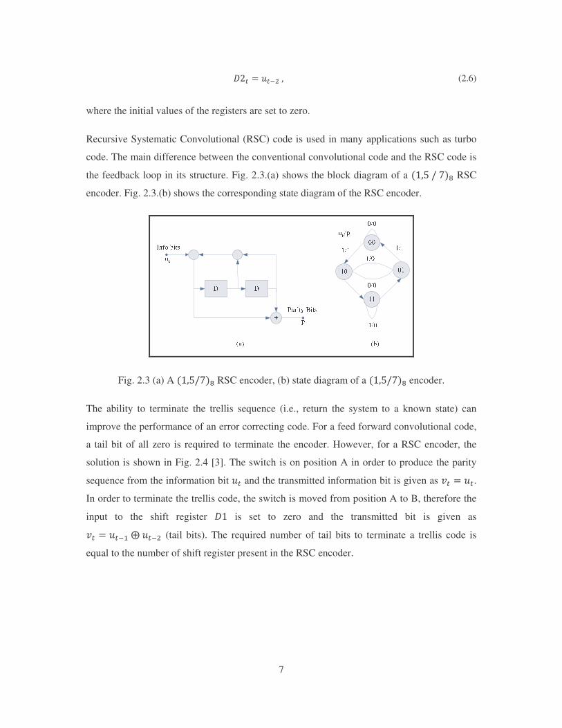
Recursive Systematic Convolutional (RSC) code is used in many applications such as turbo
code. The main difference between the conventional convolutional code and the RSC code is
the feedback loop in its structure. Fig. 2.3.(a) shows the block diagram of a �������� RSC
encoder. Fig. 2.3.(b) shows the corresponding state diagram of the RSC encoder.
Fig. 2.3 (a) A ������ RSC encoder, (b) state diagram of a ������ encoder.
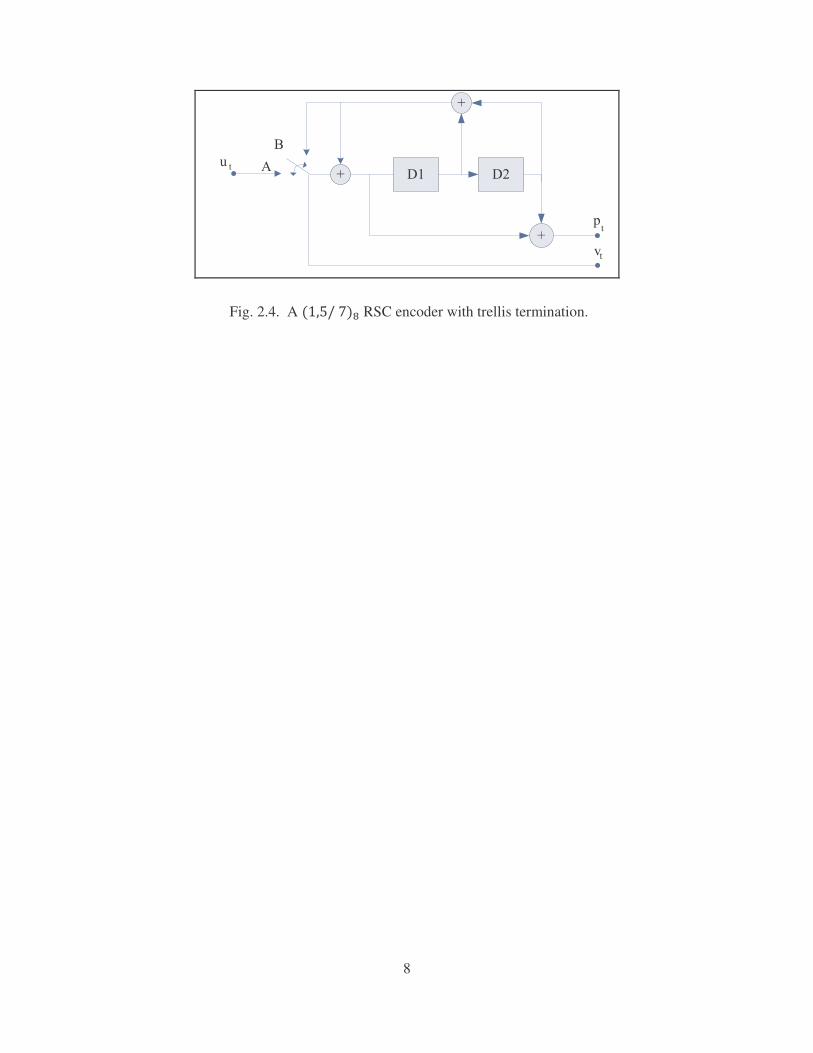
The ability to terminate the trellis sequence (i.e., return the system to a known state) can
improve the performance of an error correcting code. For a feed forward convolutional code,
a tail bit of all zero is required to terminate the encoder. However, for a RSC encoder, the
solution is shown in Fig. 2.4 [3]. The switch is on position A in order to produce the parity
sequence from the information bit �� and the transmitted information bit is given as >� � ��. In order to terminate the trellis code, the switch is moved from position A to B, therefore the
input to the shift register 4� is set to zero and the transmitted bit is given as �>� � ���.�=����! (tail bits). The required number of tail bits to terminate a trellis code is
equal to the number of shift register present in the RSC encoder.
8
�� ��
�
�
�
�
�
�
�
Fig. 2.4. A ������� RSC encoder with trellis termination.
9
Chapter 3: Turbo Trellis-Coded Modulation, Repeat-Punctured Turbo
Trellis Coded Modulation
Turbo codes and trellis-coded modulation (TCM) scheme have made huge strive forward for
the coding community. TCM scheme combined coding and modulation, results in a high
bandwidth efficient code. Then in 1993 turbo code was introduced, resulted in an exceptional
performance at low signal-to-noise ratio (SNR). Therefore it is only nature to combine both
schemes. Hence the fundamental of turbo codes and TCM are discussed below.
3.1 Turbo Code
Ever since the publication of the paper, “Mathematics description of Communication” by
Shannon, where the maximum bandwidth of an error correction code is determined by the
symbol energy. He concluded that an error correcting scheme based upon a randomised
encoder will result in a close to capacity performance [1]. However he did not suggest a
scheme that could achieve these limits. The main problem with using a randomised encoder
is that the decoding algorithm becomes complicated. In 1993 a new error correcting scheme
called turbo code was introduced by C. Berrou [2], which incorporated randomise encoding
(due to interleavers) into a structured encoder.
3.1.1 Turbo Encoder
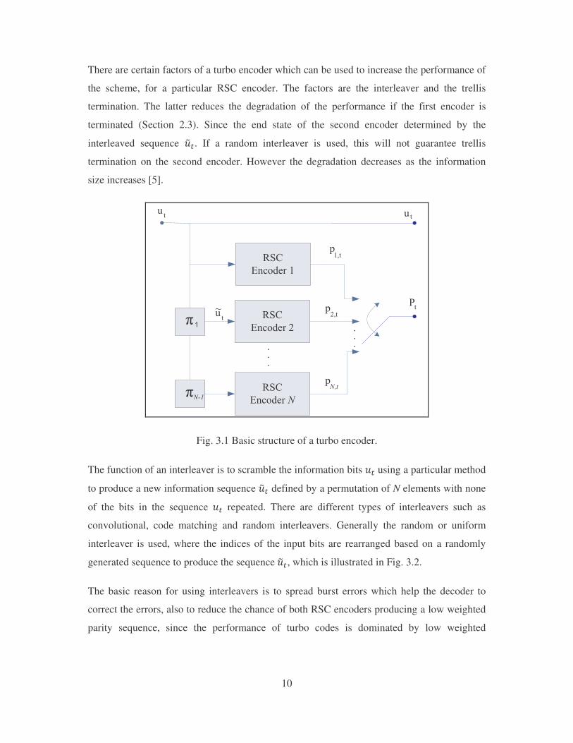
The basic structure of a turbo encoder is shown in Fig. 3.1, it consists of N parallel
concatenated RSC encoders and (N-1) interleavers �?.� @ � ?A�. [19]. Turbo codes are
sometimes known as parallel concatenated convolutional code (PCCC), which is evident in
its structure. In turbo code, an information sequence �� is passed through the first encoder,
producing a parity sequence �.��. Thereafter �� is passed through an interleaver to produce a
new information sequence �B� based upon an interleaver pattern. The new sequence �B� is then
passed through to the second encoder. This process of passing the information bits through an
interleaver to an encoder can be repeated N times. As the number of concatenation encoders
increases, the code rate decreases. Therefore to increase the rate of the overall encoder, a
puncturing scheme is used (deletion of certain bits). The parity bits �.�� @��A�� are punctured
accordingly to produce a sequence )�. Puncturing bits come with a drop in performance;
however the puncturing scheme can be optimised to reduce the performance degradation [8].
10
There are certain factors of a turbo encoder which can be used to increase the performance of
the scheme, for a particular RSC encoder. The factors are the interleaver and the trellis
termination. The latter reduces the degradation of the performance if the first encoder is
terminated (Section 2.3). Since the end state of the second encoder determined by the
interleaved sequence �B�. If a random interleaver is used, this will not guarantee trellis
termination on the second encoder. However the degradation decreases as the information
size increases [5].
� �
���������
� ��
������������
�
��
���
�
� ��
����������
��
�
��������
�
�
��������
Fig. 3.1 Basic structure of a turbo encoder.
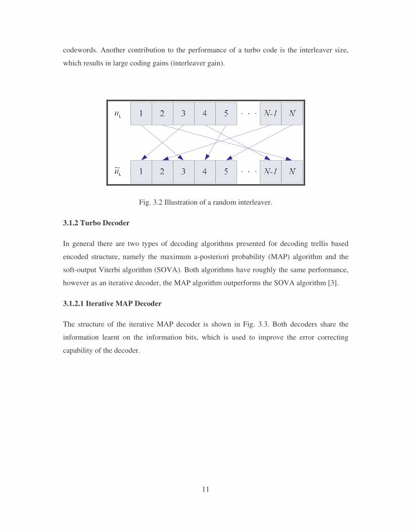
The function of an interleaver is to scramble the information bits �� using a particular method
to produce a new information sequence �B� defined by a permutation of N elements with none
of the bits in the sequence �� repeated. There are different types of interleavers such as
convolutional, code matching and random interleavers. Generally the random or uniform
interleaver is used, where the indices of the input bits are rearranged based on a randomly
generated sequence to produce the sequence��B�, which is illustrated in Fig. 3.2.
The basic reason for using interleavers is to spread burst errors which help the decoder to
correct the errors, also to reduce the chance of both RSC encoders producing a low weighted
parity sequence, since the performance of turbo codes is dominated by low weighted
11
codewords. Another contribution to the performance of a turbo code is the interleaver size,
which results in large coding gains (interleaver gain).
Fig. 3.2 Illustration of a random interleaver.
3.1.2 Turbo Decoder
In general there are two types of decoding algorithms presented for decoding trellis based
encoded structure, namely the maximum a-posteriori probability (MAP) algorithm and the
soft-output Viterbi algorithm (SOVA). Both algorithms have roughly the same performance,
however as an iterative decoder, the MAP algorithm outperforms the SOVA algorithm [3].
3.1.2.1 Iterative MAP Decoder
The structure of the iterative MAP decoder is shown in Fig. 3.3. Both decoders share the
information learnt on the information bits, which is used to improve the error correcting
capability of the decoder.
12
� ���������
���������
��
�����
��������
���
��
� �
��
�
�
��
�
�
�
�
�
� ��
� ��
� ��
� ��
� !
��"
�
��"
� !
#
#
#
#
�
�
##
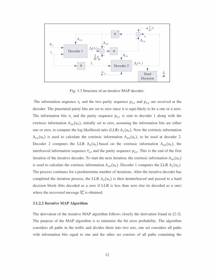
Fig. 3.3 Structure of an iterative MAP decoder.
The information sequence C� and the two parity sequence �.�� and �!�� are received at the
decoder. The punctured parity bits are set to zero since it is equi-likely to be a one or a zero.
The information bits C� and the parity sequence �.�� is sent to decoder 1 along with the
extrinsic information D.(���, initially set to zero, assuming the information bits are either
one or zero, to compute the log likelihood ratio (LLR) D.���. Now the extrinsic information D.(��� is used to calculate the extrinsic information D!(���, to be used at decoder 2.
Decoder 2 computes the LLR D!����based on the extrinsic information D!(���, the
interleaved information sequence CE.�� and the parity sequence �!��. This is the end of the first
iteration of the iterative decoder. To start the next iteration, the extrinsic information D!(��� is used to calculate the extrinsic information D.(���. Decoder 1 computes the LLR D.���. The process continues for a predetermine number of iterations. After the iterative decoder has
completed the iteration process, the LLR D!��� is then deinterleaved and passed to a hard
decision block (bits decoded as a zero if LLR is less than zero else its decoded as a one)
where the recovered message ��FFF is obtained.
3.1.2.2 Iterative MAP Algorithm
The derivation of the iterative MAP algorithm follows closely the derivation found in [2-3].
The purpose of the MAP algorithm is to minimise the bit error probability. The algorithm
considers all paths in the trellis and divides them into two sets, one set considers all paths
with information bits equal to one and the other set consists of all paths containing the
13
information bits equal to zero. Therefore it computes the log likelihood ratio of these sets,
given as
D��� � GHIJ)��� � �K�)��� � �K�L�� (3.1)
We assume that the input bit to the encoder at time , is given as ��. We assume that the RSC
encoder contains MN number of states and the state of the encoder at time , is "� corresponding to the input bit �� and the pervious state "��.. We also define the transmitted
sequence as ��� � O�.� �P� @ � �Q� @ � ��R and received sequence corrupted by noise at the
decoder as ��� � O�.� �P� @ � �Q� @ � ��R. The transmitted symbols ��.� �P� @ � �Q� @ � �� can be
broken down into the individual information and parity bits, i.e., �Q � O���.� � � � �Q�1� @ � �Q�+R, � � ��@ � �, where n represents the total number of parity and information bits in a
transmitted symbol �Q, similarly��Q � O���.� � � � �Q�1� @ � �Q�+R. The probability of receiving a
sequence ��� given a transmitted sequence ��� is
)���� K��� �SS)T��� K��� U�V� V� �� (3.2)
For a BPSK signal in an AWGN channel we get
)T��� K��� � ;�U � �W�? X���Y�Z��3![3 �� (3.3)
and
)T��� K��� � \�U � �W�? X���Y�Z]�3
14
)��� � �K��� � ^ )�"��. � $_� "� � $K����`a�`bcYd�� (3.5)
where e,� represents all state transitions caused by an information bit �� � ��at the t stage of
the trellis diagram. By applying Bayes’ theorem to (3.5) we get
)��� � �K��� � ^ )�"��. � $_� "� � $� ���)�����`a�`bcYd�� (3.6)
Similarly, we can compute the denominator in (3.1) as
)��� � �K��� � ^ )�"��. � $_� "� � $� ���)�����`a�`bcYf�� (3.7)
where e,� represents all state transitions caused by an information bit �� � ��at the t stage of
the trellis diagram. Substituting (3. 6) and (3.7) into (3.1) we get
D��� � GHIg )�"��. � $_� "� � $� ����`a�`bcYdg )�"��. � $_� "� � $� ����`a�`bcYf �� (3.8)
Now we need to determine )�"��. � $_� "� � $� ���, since we take into account a memory less
channel and the information bits are independent of each other we break up the received
sequence ��� � O��Q�����Q���Q]�� R therefore
)�"��. � $_� "� � $� ��� � )T"��. � $_� "� � $� ��Q��� �Q� �Q]�� U�� (3.9)
By applying Bayes’ theorem to (3.9) we get
15
)�"��. � $_� "� � $� ��� � )T�Q]�� K"��. � $_� "� � $� ��Q��� �QU h������������������������������ ��������)T"��. � $_� "� � $� ��Q��� �QU
� )��Q]�� K"� � $ h )T"��. � $_� "� � $� ��Q��� �QU��
(3.10)
Applying Bayes’ theorem again to (3.10) we get
)�"��. � $_� "� � $� ��� � )��Q]�� K"� � $ h )T"� � $� �QK"��. � $_� ��Q��U h ������������������������)T"��. � $_� ��Q��U�������������������������
����������������������������������� )��Q]�� K"� � $ h )�"� � $� �QK"��. � $_ h �������)T"��. � $_� ��Q��U����������
�������������������������� )��Q]�� K"� � $ h )T"��. � $_� ��Q��U h ������������������������^)��� � �� "� � $� �QK"��. � $_.
i� �
(3.11)
Now from (3.11) we define the following terms
#� �$_� $ � )�j� � �� �� � "� � $K"��. � $_�� &��$ � )��Q]�� K"� � $�� %��$ � )�"� � $� ��Q ��
(3.12)
(3.13)
(3.14)
where #� �$_� $ is known as the state transition probability, &��$ the reverse probability
function and %��$ the forward probability function. Substituting (3.12), (3.13) and (3.14)
into (3.8) we get
16
D��� � GHIg %��.�$�`a�`bcYd &��$#� �$_� $g %��.�$�`a�`bcYf &��$#� �$_� $�� (3.15)
Now we need to compute the following probabilities�%��$, &��$ and #� �$_� $. Let us start
with #� �$_� $, by applying Bayes’ theorem to (3.12), we get
#� �$_� $ � )�j� � �� �� � "� � $K"��. � $_����������������� � )�j� � �� �� � "��. � $_� "� � $)�"��. � $_ ���
(3.16)
Applying Bayes’ theorem to (3.16) we get
#� �$_� $ � )���Kj� � �� "��. � $_� "� � $ h )�j� � �� "��. � $_� "� � $)�"��. � $_ �� (3.17)
Note that moving from state "��. � $_ to the state "� � $ due to an information bit j� � � results in the transmitted bit �� at the t level of the trellis, therefore (3.17) is given as
#� �$_� $ � )���K��� )�j� � �K"��. � $_� "� � $ h )�j� � �� "��. � $_� "� � $)�"��. � $ ��� (3.18)
Finally by applying Bayes’ theorem to (3.18) we get
#� �$_� $ � )���K��� )���K"� � $� "��. � $_� )�"� � $K"��. � $_�� (3.19)
We define ���� � )�"� � $K"��. � $_ as the a-priori probability of j� � �, therefore #� �$_� $ is calculated as follows:
17
#� �$_� $ � klm���� nopq\g r���� \ �����$s!t�.�i� � ! u vwX���$_� $xe�
����������������������������������������������������������������H,wXCv�yXz����� (3.20)
where - � � represents the information bit, �����$ is the encoded output associated with the
transition from state "��. � $_ to "� � $ in the trellis and n represents the total number of
encoded bits (information plus the parity bits). Note the expression for )���K�� is
normalised by multiply (3.2) with TW�? Ut [3].
Now we compute the reverse probability &��$. Since the transition from state "� � $ to state "�]. � $_ is dependant of the received bit ��, hence (3.13) becomes
&��$ � )��Q]�� K"� � $��������������������������������������������������������������������������� �^ )��Q]�� � "�]. � $_K"� � $�{|�.
`ai� ����������������������������
(3.21)
By applying Bayes’ theorem to (3.21) we get
&��$ �^ )��Q]�� � "�]. � $_� "� � $)�"� � ${|�.`ai� ��� (3.22)
Since the received bits are independent of each other, we split the received sequence into �Q]�� � O��Q]��� �Q]P� ], hence (3.22) becomes
&��$ �^ )��Q]P� � ��]�� "�]. � $_� "� � $)�"� � ${|�.`ai� ��� (3.23)
By applying Bayes’ theorem to (3.23) we get
&��$ �^ )��Q]P� K��]�� "�]. � $_� "� � $ h )���]�� "�]. � $_� "� � $)�"� � ${|�.`ai� ����������
18
�^ )��Q]P� K"�]. � $_ h )���]�� "�]. � $_� "� � $)�"� � $ ������������������������{|�.`ai�
�^ )��Q]P� K"�]. � $_ h )���]�� "�]. � $_K"� � $ h )�"� � $)�"� � ${|�.`ai� ����
(3.24)
Note that )��Q]P� K"�]. � $_ � &�].�$_ and the probability )�"�]. � $_� ��].K"� � $ can be
computed by the summation of all possible information bits j� � � for � � �� �. Hence (3.24)
becomes
&��$ �^ &�].�$_�^ )�j�]� � �� ��]�� "�]. � $_K"� � $ b�.�� �������������{|�.`ai�
�^ &�].�$_�^ #�]. �$_� $ b�.��{|�.`ai� ������������������������������������������������
(3.25)
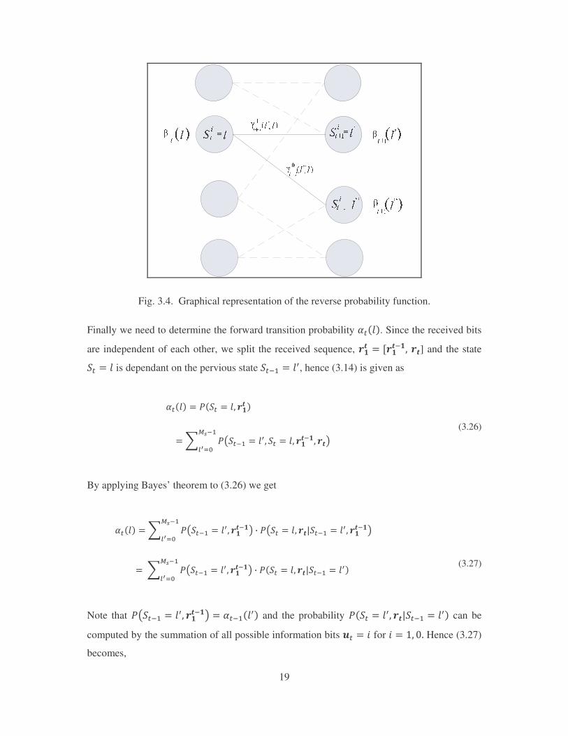
Therefore the value of &��$ is calculated recursively using (3.25) with the initial
value�&A].�� � �, assuming trellis termination and &A].�� � � for � } �. The graphical
representation of the computation of &��$ is shown in Fig. 3.4. The value &��$ for the state "� � $ at the t state of the trellis diagram is equal to the &�].�$_ value at the state "�]. � $_ multiplied by the transition probability��#�]. �$_� $, assuming there exists a connection
between the states "�]. � $_ and "� � $ [20-21].
19
Fig. 3.4. Graphical representation of the reverse probability function.
Finally we need to determine the forward transition probability %��$. Since the received bits
are independent of each other, we split the received sequence, ��Q � O��Q��� �Q] and the state "� � $ is dependant on the pervious state "��. � $_, hence (3.14) is given as
%��$ � )�"� � $� ��Q ����������������������������������������������� �^ )T"��. � $_� "� � $� ��Q��� �QU{|�.
`ai� ����� (3.26)
By applying Bayes’ theorem to (3.26) we get
%��$ �^ )T"��. � $_� ��Q��U{|�.`ai� h )T"� � $� �QK"��. � $_� ��Q��U��������������
��^ )T"��. � $_� ��Q��U{|�.`ai� h )�"� � $� �QK"��. � $_���������������
(3.27)
Note that )T"��. � $_� ��Q��U � %��.�$_ and the probability )�"� � $_� �QK"��. � $_ can be
computed by the summation of all possible information bits j� � � for � � �� �� Hence (3.27)
becomes,
20
%��$ �^ )T"��. � $_� ��Q��U{|�.`ai� ^ )�j� � �� �� � "� � $K"��. � $_ b�.�� �
�^ %��.�$_ h^ #� �$_� $ b�.��{|�.`ai� ����������������������������������������������������������
(3.28)
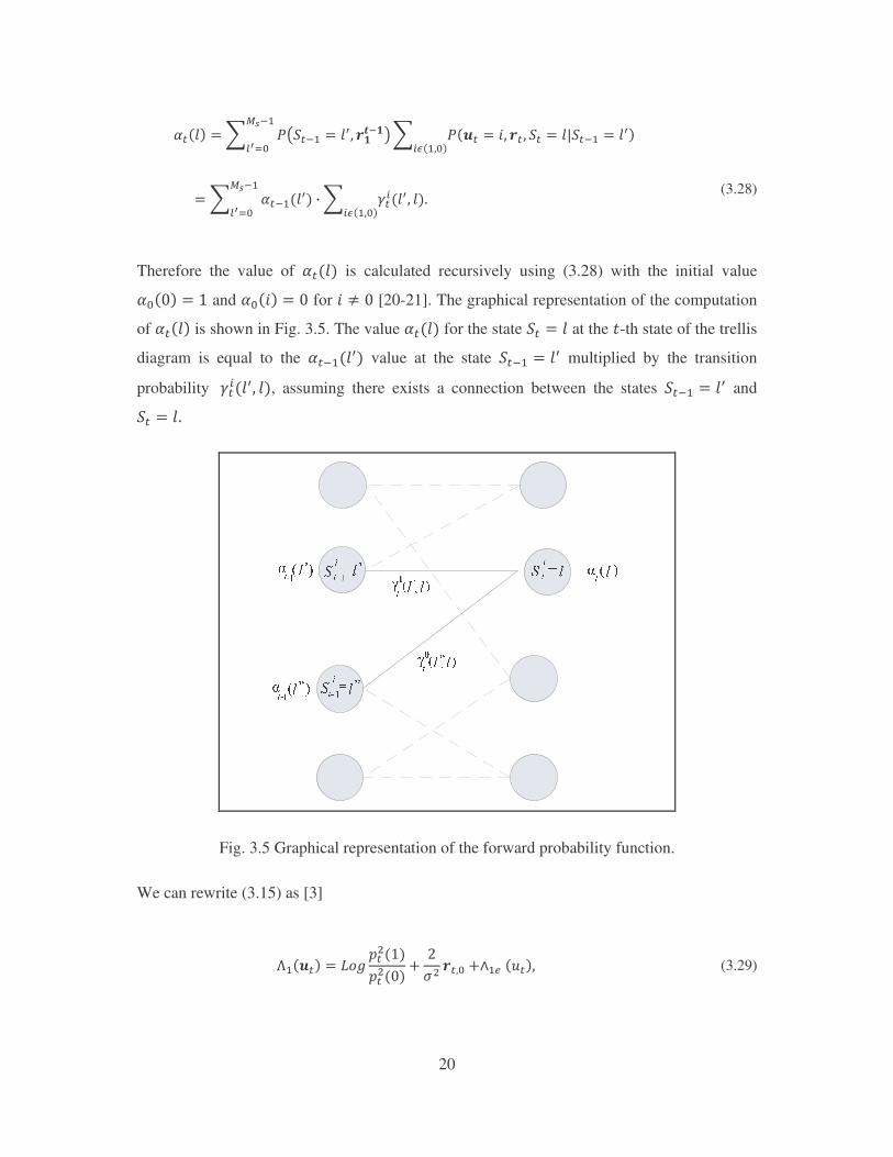
Therefore the value of %��$ is calculated recursively using (3.28) with the initial value %��� � � and %��� � � for � } � [20-21]. The graphical representation of the computation
of %��$ is shown in Fig. 3.5. The value %��$ for the state "� � $ at the ,-th state of the trellis
diagram is equal to the %��.�$_ value at the state "��. � $_ multiplied by the transition
probability �#� �$_� $, assuming there exists a connection between the states "��. � $_ and "� � $�
Fig. 3.5 Graphical representation of the forward probability function.
We can rewrite (3.15) as [3]
D.�j� � GHI��!����!�� ; � ! ���� ;~.( ���� (3.29)
21
where ��!�� is the probability of �� � ����� �,��� is the probability of �� � � at decoder 2
and ~.( ��� represents the extrinsic information of decoder 1 which is given as
~.( �j� � GHIg %��.�$_&��$_{|`�`ai. X:� �g TC��� \ :���U!t�.�i. � ! �g %��.�$_&��$_{|`�`ai� X:� �g TC��� \ :���U!t�.�i. � ! �� (3.30)
Since the second decoder includes the received soft information�����. Hence the contribution
due to the received information must be removed from ~. ���. Since ~.( ��� does not
contain the received information C���, it can be used as the a-priori probability for the second
decoder, i.e.,
~.( �j� � $HI��!����!��� (3.31)
It can be shown that the a-priori probability ��!�� and ��!�� is given as [6]
��!�� � X~d��jY� ; X~d��jY�� (3.32)
and
��!�� � �� ; X~d��jY�� (3.33)
Now we have to determine the extrinsic information ~.( ��� and ~!( ��� from the MAP
algorithm as follows:
~.( ��� � D.��� \ � ! ���� \~!( ��� (3.34)
and
22
~!( ��� � D!��� \ � ! ���� \~.( ���� (3. 35)
We now extend the iterative decoder for a Rayleigh flat fading channel with the channel state
information (CSI) known at the decoder. The forward and reverse recursive probability
function %��$ and &��$ are determined using the modified transition probability #� �$_� $ , for a fading channel #� �$_� $, which is given as [3]
#� �$_� $ � klm���� nopq\g r���� \ %������$s!t�.�i� � ! u vwX���$_� $xe�
����������������������������������������������������������������H,wXCv�yXz����� (3.36)
where %/represents the fading coefficient. Following a similar derivation above, LLR of the
information bit for a fading channel can be decomposed to the form
D.�j� � GHI�������� ; � ! %����� ;~.( ���� (3. 37)
where the extrinsic information ~.( ��� is given as
~.( �jQ � GHIg %��.�$_&��$_{|`�`ai. X:� �g TC��� \ %�:���U!t�.�i. � ! �g %��.�$_&��$_{|`�`ai� X:� �g TC��� \ %�:���U!t�.�i. � ! ��� (3. 38)
Following a similar derivation to (3.34), we determine the extrinsic information ~.( ��� as
follows:
~.( ��� � D.��� \ � ! ������ \~!( ����� (3.39)
and
23
~!( ��� � D!��� \ � ! ������ \~.( ���� (3.40)
The iterative MAP decoder is summarised as,
1. We set ~.( ��� � � since we assume the information bit �� is equi-likely to be zero or
one.
2. Compute ~. ��� using the MAP algorithm, using (3.15).
3. Use (3.35) to compute ~!( ��� for decoder 2.
4. Compute ~! ��� using the MAP algorithm, using (3.15).
5. Use (3.34) to compute ~.( ��� for decoder 1.
6. Repeat steps 2 to 5 for � number of times which is set for the decoder.
7. After � iteration, apply a hard decision on LLR ~! ��� of decoder 2.
3.2 Trellis Coded Modulation
The Trellis Coded Modulation (TCM) scheme was developed by Ungerboeck in 1982 [22]. It
was a breakthrough for communication systems in bandwidth limited channels. It is a
combination of coding and modulation, where the coding section is made up of convolutional
codes (or trellis codes) along with multilevel/phase signal modulation. Hence TCM scheme
incorporates the spectrum efficiency brought on by signal modulations with the error
correctional capability of trellis codes. This results in coding gain without bandwidth
expansion.
3.2.1 Encoder
In general the TCM scheme takes a rate K/(K+1) encoder, where K is the number of
information bits, and an M-ary signal mapper that maps �8 input bits into a larger �8].
constellation points. The structure of a TCM scheme is shown in Fig. 3.6. It consists of a
basic rate 1/2 ��� � convolutional code with an overall encoding rate of 2/3. The
24
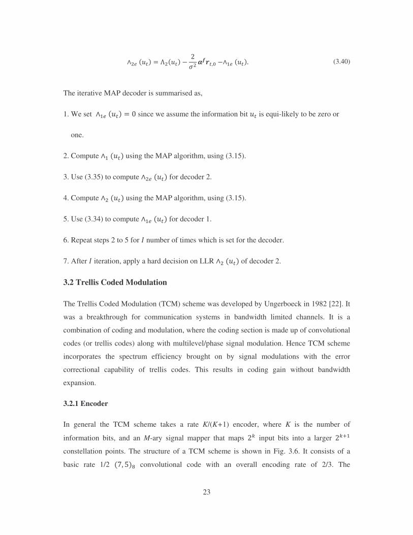
information bits as well as the encoded bits are sent to a constellation mapper, in this case the
modulation scheme is an 8PSK.
� �
��
�
��
��
� ��
$�� %�
&���'����
���
�
(
(
�
)
(�
Fig. 3.6. A rate of 2/3 TCM encoder.
The two information bits �.�� and �!�� enter the TCM encoder. The first information bit �.�� is
left uncoded. The second information bit �!�� is passed through a ��� � convolutional code
to produce two parity bits �.�� and��!��. Thereafter the bits �.��, �.�� and �!�� are mapped to an
8PSK modulation scheme. Note that the information bit �.�� is left uncoded, since it is the
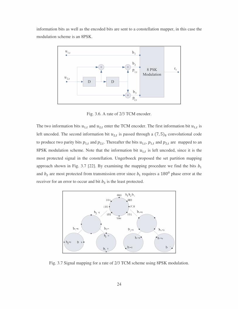
most protected signal in the constellation. Ungerboeck proposed the set partition mapping
approach shown in Fig. 3.7 [22]. By examining the mapping procedure we find the bits �.
and �! are most protected from transmission error since �. requires a ���� phase error at the
receiver for an error to occur and bit �� is the least protected.
Fig. 3.7 Signal mapping for a rate of 2/3 TCM scheme using 8PSK modulation.
25
3.2.2 Decoder
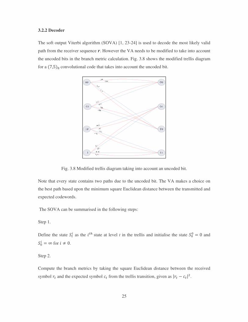
The soft output Viterbi algorithm (SOVA) [1, 23-24] is used to decode the most likely valid
path from the receiver sequence �� However the VA needs to be modified to take into account
the uncoded bits in the branch metric calculation. Fig. 3.8 shows the modified trellis diagram
for a �����convolutional code that takes into account the uncoded bit.
Fig. 3.8 Modified trellis diagram taking into account an uncoded bit.
Note that every state contains two paths due to the uncoded bit. The VA makes a choice on
the best path based upon the minimum square Euclidean distance between the transmitted and
expected codewords.
The SOVA can be summarised in the following steps:
Step 1.
Define the state "� as the ��'�state at level t in the trellis and initialise the state "�� � � and "� � � for � } �.
Step 2.
Compute the branch metrics by taking the square Euclidean distance between the received
symbol C� and the expected symbol �� from the trellis transition, given as KC� \ ��K!.

26
Step 3
Compute the state metric at the state "� at the ,�stage by adding the branch metric to the
previous state at the stage�, \ �.
Step 4.
Compare the state metric at the , stage for all the paths entering the state "� . Select the path
that results in the smallest square Euclidean distance and store the surviving path as well as
its metric value.
Step 5
After completing steps 2 to 4 for , � �� � � � �, where N represents the number of information
bits, the information bits are determined by selecting the path in the trellis sequence that
results in the smallest square Euclidean distance.
27
Chapter 4: Performance Analysis of a Turbo Trellis-Coded Modulation
and Repeat-Punctured Turbo Trellis-Coded Modulation Scheme
In order to confirm the simulation results of the TTCM and RPTTCM schemes at high SNR
we need to compute the probability of error, also to predict the performance at high SNR.
There are various methods developed to calculate the performance of TTCM system [11-12,
25-26]. In [25], the performance bound was computed base on the calculating the expected
number of codwords and the distance profile and in [12] obtained the performance bound
using the union bound approach. Certain methods however have either complexity or
computational issues. Therefore we use the method developed in [25] to derive the bounds,
since it is quick and accurate when certain approximations are made.
4.1 Derivation of the Performance Bound for a TTCM scheme in an AWGN channel
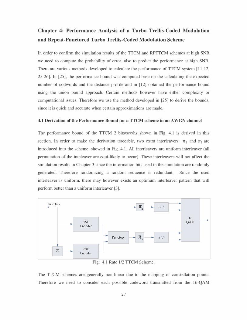
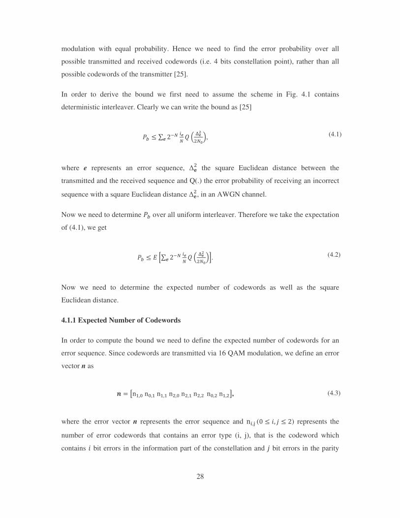
The performance bound of the TTCM 2 bits/sec/hz shown in Fig. 4.1 is derived in this
section. In order to make the derivation traceable, two extra interleavers ?. and ?!�are
introduced into the scheme, showed in Fig. 4.1. All interleavers are uniform interleaver (all
permutation of the inteleaver are equi-likely to occur). These interleavers will not affect the
simulation results in Chapter 3 since the information bits used in the simulation are randomly
generated. Therefore randomizing a random sequence is redundant. Since the used
interleaver is uniform, there may however exists an optimum interleaver pattern that will
perform better than a uniform interleaver [3].
Fig. 4.1 Rate 1/2 TTCM Scheme.
The TTCM schemes are generally non-linear due to the mapping of constellation points.
Therefore we need to consider each possible codeword transmitted from the 16-QAM
28
modulation with equal probability. Hence we need to find the error probability over all
possible transmitted and received codewords (i.e. 4 bits constellation point), rather than all
possible codewords of the transmitter [25].
In order to derive the bound we first need to assume the scheme in Fig. 4.1 contains
deterministic interleaver. Clearly we can write the bound as [25]
)* � g ��A �A � r ��3!Afs� , (4.1)
where e represents an error sequence, *�! the square Euclidean distance between the
transmitted and the received sequence and Q(.) the error probability of receiving an incorrect
sequence with a square Euclidean distance *�!, in an AWGN channel.
Now we need to determine )* over all uniform interleaver. Therefore we take the expectation
of (4.1), we get
)* � � �g ��A �A � r ��3!Afs� �. (4.2)
Now we need to determine the expected number of codewords as well as the square
Euclidean distance.
4.1.1 Expected Number of Codewords
In order to compute the bound we need to define the expected number of codewords for an
error sequence. Since codewords are transmitted via 16 QAM modulation, we define an error
vector n as
+ � ��.������.��.�.��!����!�.��!�!�����!��.�!�, (4.3)
where the error vector n represents the error sequence and � ���(� � �� - � �) represents the
number of error codewords that contains an error type (i, j), that is the codeword which
contains � bit errors in the information part of the constellation and - bit errors in the parity
29
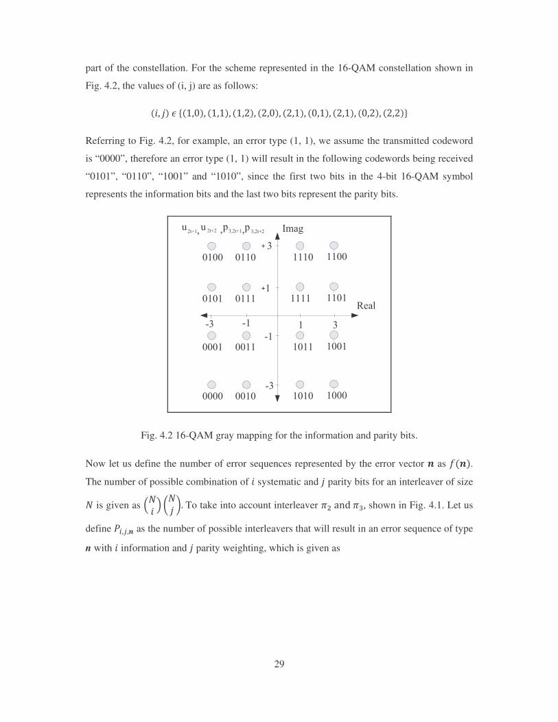
part of the constellation. For the scheme represented in the 16-QAM constellation shown in
Fig. 4.2, the values of (i, j) are as follows:
��� -�x������� ����� ����� ����� ����� ����� ����� ����� ����� Referring to Fig. 4.2, for example, an error type (1, 1), we assume the transmitted codeword
is “0000”, therefore an error type (1, 1) will result in the following codewords being received
“0101”, “0110”, “1001” and “1010”, since the first two bits in the 4-bit 16-QAM symbol
represents the information bits and the last two bits represent the parity bits.
+�++ +��+ ���+ ��++
+�+� +��� ���� ��+�
+++� ++�� �+�� �++�
++++ ++�+ �+�+ �+++
)#) �#�
)
#)
�
#�
����
)����
����)����
� � � ,-�.
���'
�
�
Fig. 4.2 16-QAM gray mapping for the information and parity bits.
Now let us define the number of error sequences represented by the error vector + as /�+. The number of possible combination of � systematic and - parity bits for an interleaver of size
� is given as r�� s J�- L��To take into account interleaver ?!�����?�� shown in Fig. 4.1. Let us
define ) ���+ as the number of possible interleavers that will result in an error sequence of type
n with � information and - parity weighting, which is given as
30
) ���+ � J �y�����@�����L ������������������������� ������� ���/ ������;�����;������;������;�������;���� � ������;�����;������;�����;�������;����� � � z�������������������������������������������������������������������������������������� H,wXCv�yX ,
(4.4)
where the term J �N�.���@��!�!L�represents the total number of possible locations of the error
type (i, j) among the �N transmitted symbol. For example if we assume that a 100
constellation points (�N� � ���) are transmitted over a noise channel and we get a single bit
error at the receiver. Lets assume for all error types (i, j) the value of � �� � � except for �.��� � �, i.e., there exists one information bit error in one constellation point out of the
�N�transmitted points. Therefore the single error type can occur in r���� s � ��� positions in
the transmitted sequence. The term ��d�f� @���d�f� represents the possible locations of the
information bits and the parity bits for an error type (i, j) within a codeword. For example, for
an error type (1, 0) there are two possible locations for the error bits in the codeword, “0100”
and “1000” assuming “0000” is transmitted. Therefore if there is �.����number of error type
(1, 0), there are ��d�f�possible locations for the information bits of the error type (1, 0). Finally
the expected weight enumerating function ���� - of the encoder in Fig. 4.1 is given as
���� - � g �d� ��dh�3� ��3rA s�d��3�N���i�d]�3 , (4.5)
where i represents the number of information bits, -. and -! represents the number of parity
bits subject to (- � -. ; -!) from encoder 1 and 2, respectfully and ,8��� -8�represents the
number of codewords with � information bits and -8 parity bits for the ��' encoder (Appendix
A). The expected number of error sequences for an error vector n is given as �A/�+��Where /�+ is given as
/�+ � g ���� - �Z���+rA srA� s �� �, (4.6)
and �A represents the possible number of codewords for a message length of �.
31
4.1.2 Determining the Square Euclidean Distance
Now we need to determine 4+, the square Euclidean distance caused by the error sequence
represented by the error vector n, where 4+ is given as
4+ � 0+��! @ 0+�8¡!�. @ �8¡ ¢, (4.7)
where �t is the number of possible error distance caused by the error vector +, 0+�1! is the
square Euclidean distance and � is the probability that the error sequence represented by +
will result in a square Euclidean distance of 0+�1! occurring.
In order to determine 4+ for an error sequence represented by +. We first assume that all
constellation points in the 16-QAM system are equi-likely to occur. Therefore for each error
type (i, j) there exists a distance profile given as
41�5 � £0�! @ 08Z��!�. @ �8Z�� ¤. (4.8)
For each possible distance of a particular error type (i, j) we need to calculate � the
probability that the distance 0 ! will occur for a given error type. The term � is given by
� � ¥013¦ , (4.9)
where 2013 represents the total number of received codewords that will result in a distance 01!
and § represents the total number of received codewords for an error type (i, j). For example
to calculate the distance profile for the error type (1, 0), i.e., 41�5. We first assume that one
codeword “0000” is transmitted. Hence the received codewords that results in an error type
(1, 0) for the 16 QAM mapping are “0100” and “1000”. The square Euclidean distance
between “0000” and “0100” is 4 and between “0000” and “1000” is 16. Thereafter we take
into account all other codewords in the 16-QAM constellation. The total number of
codewords that results in a square Euclidean distance of 4 is 32 and the distance of 16 is 32.
32
The total number of codewords that results in an error type (1, 0) is 64. Hence the probability
of the square Euclidean distance of 4 occurring for an error type (1,0) is �. � �!�7 � ���.
Similarly for the square Euclidean distance of 16 we get��! � ���. Therefore the distance
profile for the error type (1, 0) is given as
4.�� � � ¨ �©��� ����.
Finally we need to determine the overall error distance 4+ for the error vector + from the
distance profiles 41�5 discussed above. 4+ is calculated from 41�5 as follows:
4+ � 4��.tf�d ª 4.�.td�d ª @�ª�4!�!t3�3 , (4.10)
where 4 ��8 represents the �-fold cross multiplication of 41�5 with itself. The multiplication
between any error profile is shown in [25].
Assume there exist two error profiles
4. � �0�!�. �����0!!�! ���@@����08d!�8d ¢,
and
4! � £�0�_!�._ �����0!_!�!_ ���@@����083_!�83_ ¤,
then
4. ª 4! � £�0�!;0�_!�.� �._ ���0�!;0P_!�.� �!_ ����@@���08d! ;083_!�8d � �83_ �¤. (4.11)
The product of two distance profiles is equal to the sum of the individual square Euclidean
distance and the product of the corresponding probability�� .
33
From Section 4.1.1, we found that the expected number of error sequence for the error vector
n as �A/�+. Therefore the expected number of error sequence that results in a square
Euclidean distance 0+�1! is � �A/�+. Now we are in a position to compute expectation of
(4.1) as
)* �^^^@^^ ��/�+� � «¬+�!���®8¡8
A|t3�3
A|td�f
A�
A � (4.12)
4.1.3 Results
The system shown in Fig. 4.1 was simulated and compared with the performance bound
derived above. There are certain assumptions we make to decrease the computation
complexity of (4.12). We show that these assumptions results in a very close approximation
of the complete bound. By examining the summation of all the error term � ��, we find that
there exists a natural upper bound. Assuming that there are � information bits in errors, the
upper bound for the error term �.�� is � if � is less than �N . It follows that the upper bound for
the summation for the term �!�� is �td�f! and the upper bound of the rest of the error term,
follows suit. The upper bound for the error term reduces the computation of (4.12). However
this works well for short length codes (N<50). Therefore we need to make a few more
assumptions.
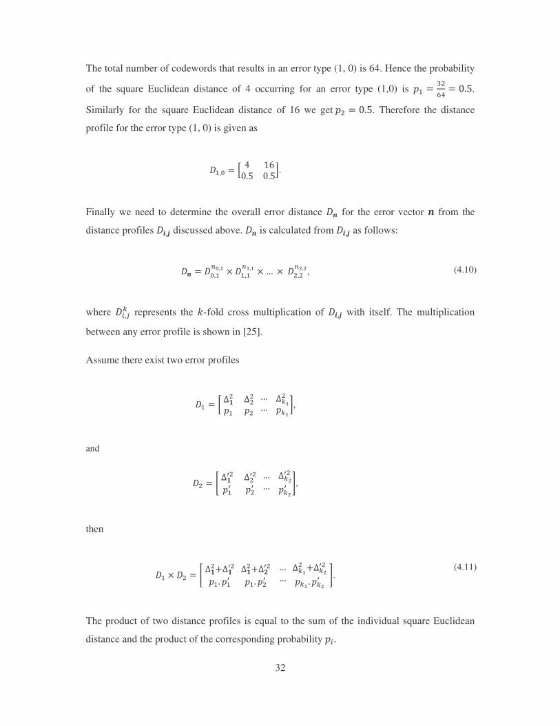
The performance of the TTCM scheme in Fig. 4.1 at high SNR is dominated by the terms �.�� and ���.. Since these terms represent a single bit error with a minium error distance in
the 16-QAM constellation. Fig. 4.3 shows the effect of computing (4.12) using various
number of error terms.
Since more error terms are used to evaluate, this severely increases the run-time of the code
for large information size. By examining Fig. 4.3 we found that the use of extra error term
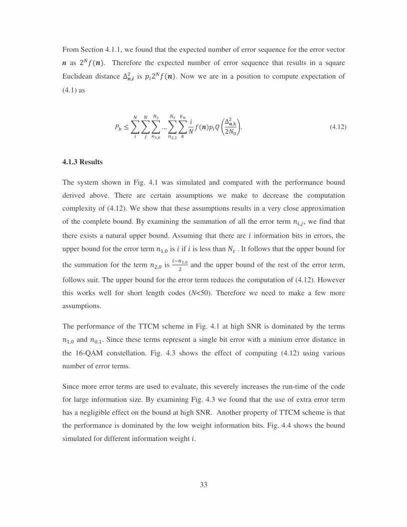
has a negligible effect on the bound at high SNR. Another property of TTCM scheme is that
the performance is dominated by the low weight information bits. Fig. 4.4 shows the bound
simulated for different information weight �.
34
Fig. 4.3 Performance bound for a TTCM scheme in an AWGN channel for different number
of error terms � ��.
Fig. 4.4 Performance bound of the TTCM scheme in an AWGN channel using information
weight of � � �� � � ��and � � ��
2 4 6 8 10 12
10-10
10-8
10-6
10-4
10-2
Eb/No (dB)
BE
R
2 terms4 terms
2 4 6 8 10 12
10-10
10-8
10-6
10-4
10-2
BE
R
Eb/No (dB)
i=5i=3i=10
N =200
35
Again we find the bound converges at high SNR. We use these assumptions for codes with
large information length.
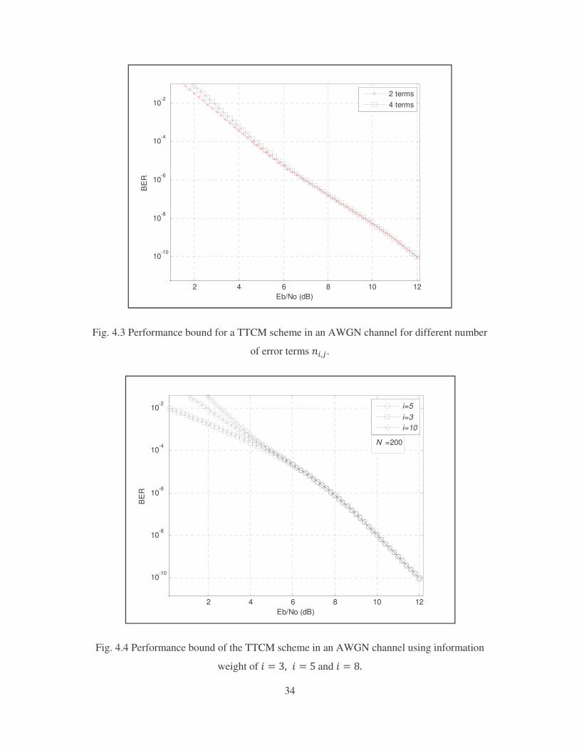
Fig. 4.5 compares the simulation results of the TTCM scheme from Fig. 4.1, for an
information size of �=200, using the iterative MAP decoder to determine the information
bits, with the iteration number set to 18 and the number of error frame set to 80. The
simulation is compared with the performance bound of (4.12). The computation of the
performance bound for an information size��=200, using an information weight �=10, we
found the bound matches the simulations results at high SNR values.
Fig. 4.5 Simulation results and performance bound of a TTCM scheme for N=200 in an
AWGN channel.
4.2 Derivation of the Performance Bound for RPTTCM in an AWGN channel
The bound for the repeat-puncture turbo trellis-coded modulation (RPTTCM) scheme shown
in Fig. 4.6 is derived. The bounds for the RPTTCM system follow the same derivation as the
bound for the AWGN channel in Section 4.1.
3 4 5 6 7 8 9 10 11 12
10-10
10-8
10-6
10-4
10-2
Eb/No (dB)
BE
R
Performance BoundSimulation Result
N =200
36
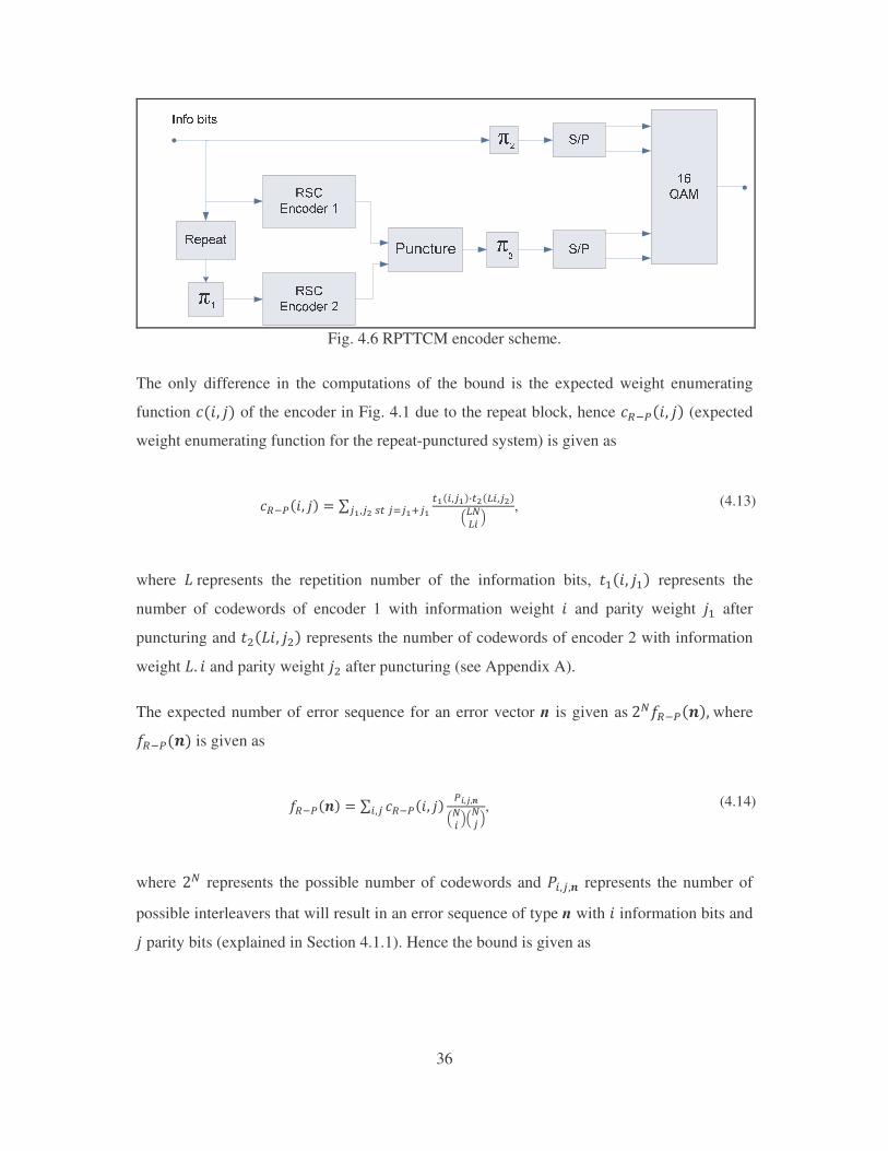
Fig. 4.6 RPTTCM encoder scheme.
The only difference in the computations of the bound is the expected weight enumerating
function ���� - of the encoder in Fig. 4.1 due to the repeat block, hence �¯����� - (expected
weight enumerating function for the repeat-punctured system) is given as
�¯����� - � g �d� ��dh�3�° ��3r°A° s�d��3�N���i�d]�d , (4.13)
where G�represents the repetition number of the information bits, ,.��� -. represents the
number of codewords of encoder 1 with information weight � and parity weight -. after
puncturing and ,!�G�� -! represents the number of codewords of encoder 2 with information
weight G� � and parity weight -! after puncturing (see Appendix A).
The expected number of error sequence for an error vector n is given as��A/̄ ���+��where /̄ ���+ is given as
/̄ ���+ � g �¯����� - �Z���+rA srA� s �� , (4.14)
where �A represents the possible number of codewords and ) ���+ represents the number of
possible interleavers that will result in an error sequence of type n with � information bits and - parity bits (explained in Section 4.1.1). Hence the bound is given as
37
)* �^^^@^^ �� /̄ ���+� � «¬+�!���®8¡8
A|t3�3
A|td�f
A�
A � (4.15)
The calculation of the error distance *+�! is the same for the original TTCM system shown in
Fig. 4.1 (discussed in section 4.1.2). Since both the TTCM and RPTTCM schemes shown in
Fig. 4.1 and 4.6 respectfully have the same code rate of � �< and are transmitted via a 16-
QAM constellation.
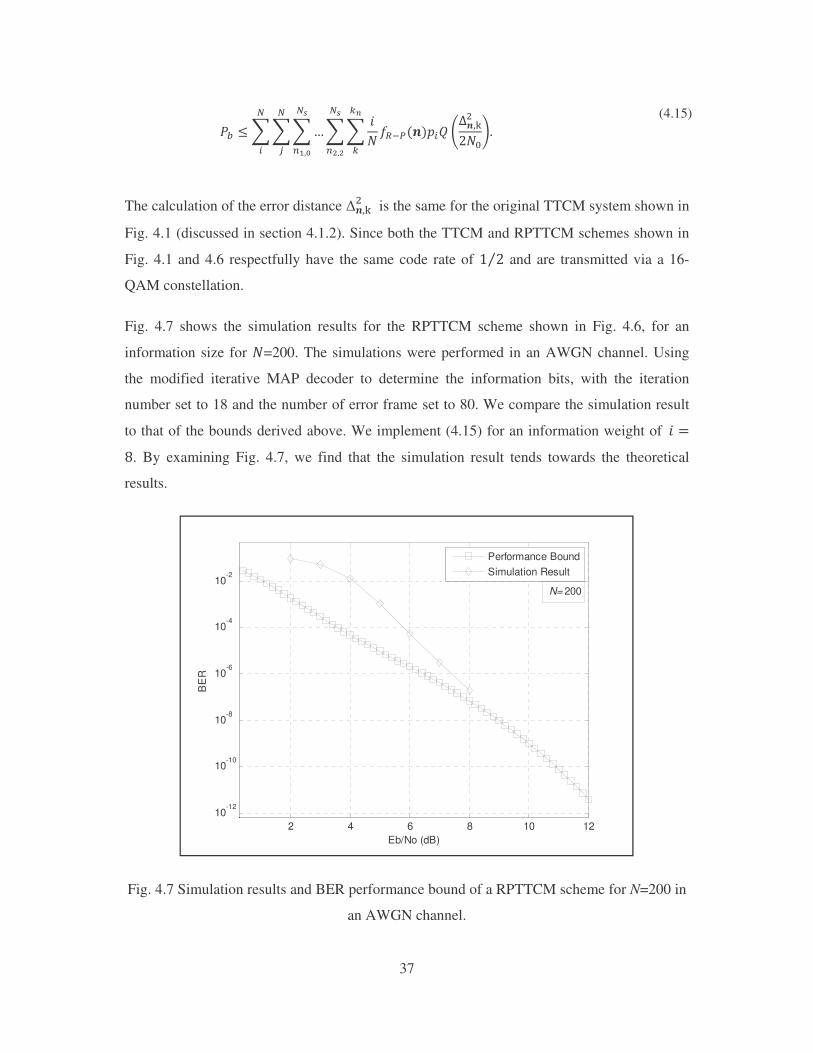
Fig. 4.7 shows the simulation results for the RPTTCM scheme shown in Fig. 4.6, for an
information size for �=200. The simulations were performed in an AWGN channel. Using
the modified iterative MAP decoder to determine the information bits, with the iteration
number set to 18 and the number of error frame set to 80. We compare the simulation result
to that of the bounds derived above. We implement (4.15) for an information weight of��� ��. By examining Fig. 4.7, we find that the simulation result tends towards the theoretical
results.
Fig. 4.7 Simulation results and BER performance bound of a RPTTCM scheme for N=200 in
an AWGN channel.
2 4 6 8 10 1210
-12
10-10
10-8
10-6
10-4
10-2
Eb/No (dB)
BE
R
Performance BoundSimulation Result
N= 200
38
4.3 Derivation of the Performance Bound in a Rayleigh Flat Fading channel
In this section, we discuss the performance bound in a Rayleigh flat fading channel. We
derive the performance of the scheme shown in Fig. 4.1. To derive the performance we again
need to make a few assumptions. Firstly we assume that the channel state information (CSI)
is known at the receiver. We also assume that the average bit energy is normalised to ��* for
the 2bits/sec/Hz 16-QAM system and the expected values of the sequence of the fading
coefficients are normalised to unity. The variance of the noise term is denoted by �� �< .
4.3.1 Performance Bound of TTCM scheme
The performance bound for the fading channel is similar to the derivation of the bound for the
AWGN channel with respect to the expected value of the codeword, i.e. �A/�+ (derived in
Section 4.1.1). The difference between both channels is the computation of the probability of
error due to an error sequence. Let assume that the transmitted sequence is :� and the
received sequence is :±. Therefore we need to compute )�:�� :±K%�(where % represent the
fading coefficient), which is bounded by [3, 11, 27]
)�:� � :±K% � �S �� ; �¨�� ²:�� \ :±� ²! � �A| i. (4.16)
where K:� \ :± K! represents the square Euclidean distance between the ��'�transmitted and
received codeword. Hence the bound is given as
)* �^^^@^^ ��/�+� S ��; �¨�� ²:�� \ :±� ²!A| i.
8¡8
A|t3�3
A|td�f
A� � �A
(4.17)
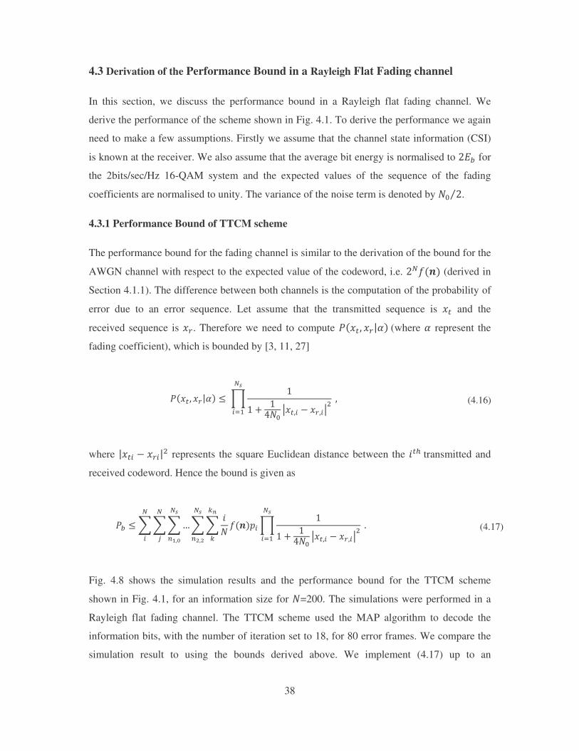
Fig. 4.8 shows the simulation results and the performance bound for the TTCM scheme
shown in Fig. 4.1, for an information size for �=200. The simulations were performed in a
Rayleigh flat fading channel. The TTCM scheme used the MAP algorithm to decode the
information bits, with the number of iteration set to 18, for 80 error frames. We compare the
simulation result to using the bounds derived above. We implement (4.17) up to an
39
information weight of �=8. We find that the performance bound matches the simulation
results at high SNR values.
Fig. 4.8 Simulation results and BER performance bound of a TTCM scheme for N=200 in a
Rayleigh flat fading channel.
4.3.2 Performance Bound of RPTTCM scheme
Just like the performance of the TTCM scheme for a Rayleigh flat fading channel, the
probability of error due to the error sequence )�:�� :±K% is the same as (4.16).
The only difference in the computation of the bound is the expected weight enumerating
function ���� - of the encoder in Fig. 4.6 due to the repeat block, hence �¯����� - (expected
weight enumerating function for the repeat-punctured system) is given as
�¯����� - � ^ ,.��� -.� ,!�G�� -!rG�G� s�d��3�N���i�d]�d � (4.18)
4 6 8 10 12 14 16
10-7
10-6
10-5
10-4
10-3
10-2
10-1
Eb/No (dB)
BE
R
Performance BoundSimulation Result
N =200
40
where G�represents the repetition number of the information bit, ,.��� -. represents the
number of codewords of encoder 1 with information weight � and parity weight -. after
puncturing and ,!�G�� -! represents the number of codewords of encoder 2 with information
weight G� and parity weight -! after puncturing (see Appendix A).
The expected number error sequence for an error vector n is given as��A/̄ ���+, where /̄ ���+ is given as
/̄ ���+ �^�¯����� - ) ���+r�� s J�- L �� � (4.19)
where ) ���+ represents the number of different interleavers that will result in an error
sequence of type n with � information and - parity weighting (explained in Section 4.1.1).
Hence the performance bound for the RPTTCM scheme is given as
)* �^^^@^^ �� /̄ ���+� S ��; �¨�� ²:�� \ :±� ²!A| i.
8¡8
A|t3�3
A|td�f
A�
A ��
(4.20)
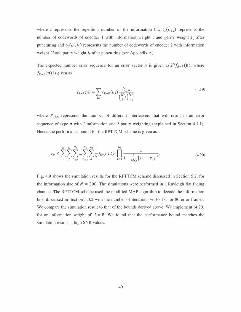
Fig. 4.9 shows the simulation results for the RPTTCM scheme discussed in Section 5.2, for
the information size of � � ���. The simulations were performed in a Rayleigh flat fading
channel. The RPTTCM scheme used the modified MAP algorithm to decode the information
bits, discussed in Section 5.3.2 with the number of iterations set to 18, for 80 error frames.
We compare the simulation result to that of the bounds derived above. We implement (4.20)
for an information weight of �� � �. We found that the performance bound matches the
simulation results at high SNR values.
41
Fig. 4.9 Simulation results and BER performance bound of a RPTTCM (L=2) scheme for
N=200 in a Rayleigh flat fading channel.
4.4 Comparison of the Performance Bound for the TTCM and RPTTCM
Scheme.
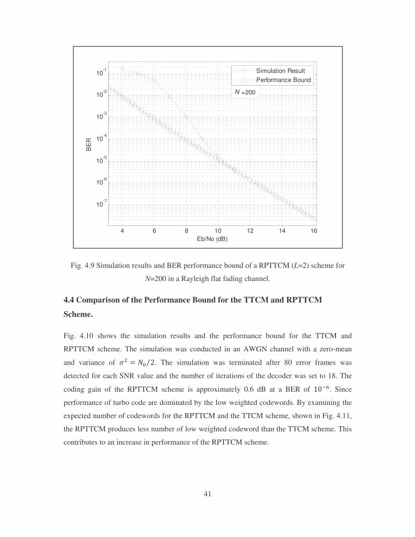
Fig. 4.10 shows the simulation results and the performance bound for the TTCM and
RPTTCM scheme. The simulation was conducted in an AWGN channel with a zero-mean
and variance of ! � �� �< . The simulation was terminated after 80 error frames was
detected for each SNR value and the number of iterations of the decoder was set to 18. The
coding gain of the RPTTCM scheme is approximately 0.6 dB at a BER of ����. Since
performance of turbo code are dominated by the low weighted codewords. By examining the
expected number of codewords for the RPTTCM and the TTCM scheme, shown in Fig. 4.11,
the RPTTCM produces less number of low weighted codeword than the TTCM scheme. This
contributes to an increase in performance of the RPTTCM scheme.
4 6 8 10 12 14 16
10-7
10-6
10-5
10-4
10-3
10-2
10-1
Eb/No (dB)
BE
R
Simulation ResultPerformance Bound
N =200
42
Fig. 4.10 Performance bound and simulation result for a RPTTCM and TTCM scheme for an
information size N=200 in an AWGN channel.
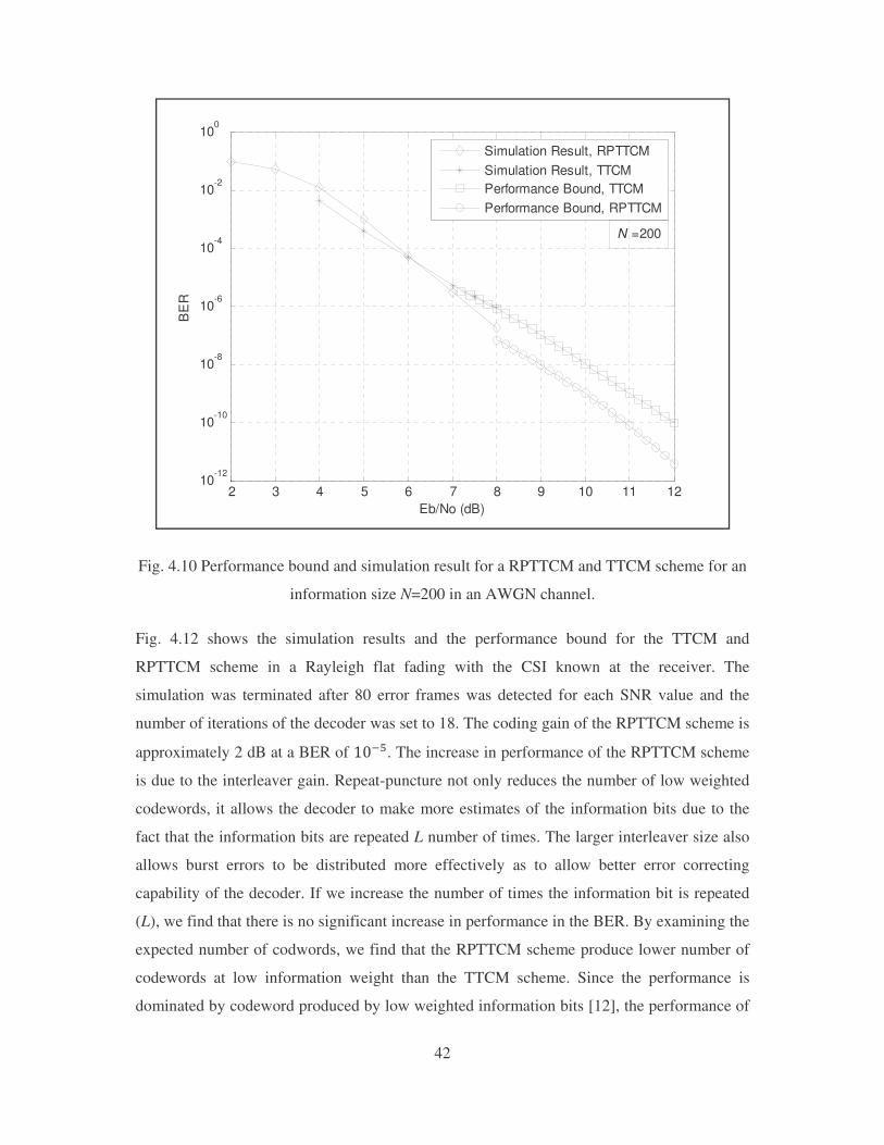
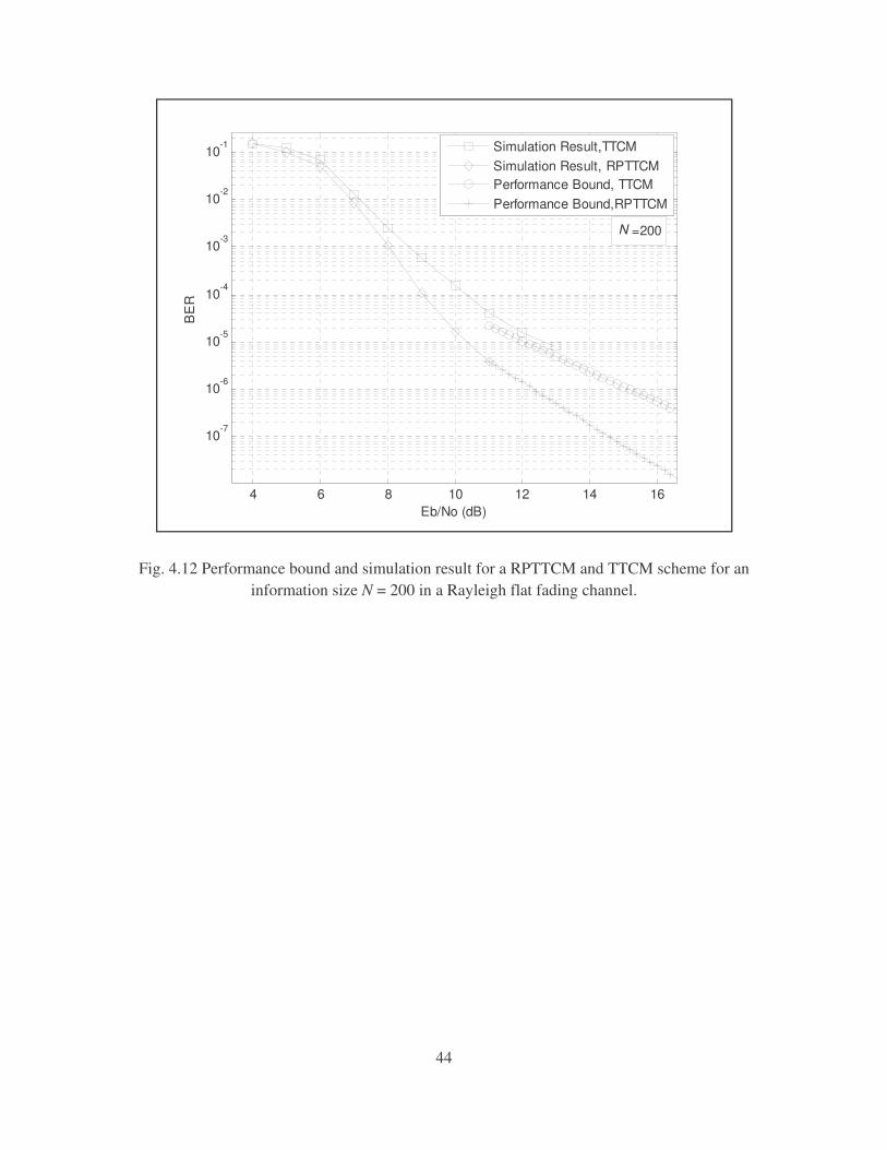
Fig. 4.12 shows the simulation results and the performance bound for the TTCM and
RPTTCM scheme in a Rayleigh flat fading with the CSI known at the receiver. The
simulation was terminated after 80 error frames was detected for each SNR value and the
number of iterations of the decoder was set to 18. The coding gain of the RPTTCM scheme is
approximately 2 dB at a BER of ���6. The increase in performance of the RPTTCM scheme
is due to the interleaver gain. Repeat-puncture not only reduces the number of low weighted
codewords, it allows the decoder to make more estimates of the information bits due to the
fact that the information bits are repeated L number of times. The larger interleaver size also
allows burst errors to be distributed more effectively as to allow better error correcting
capability of the decoder. If we increase the number of times the information bit is repeated
(L), we find that there is no significant increase in performance in the BER. By examining the
expected number of codwords, we find that the RPTTCM scheme produce lower number of
codewords at low information weight than the TTCM scheme. Since the performance is
dominated by codeword produced by low weighted information bits [12], the performance of
2 3 4 5 6 7 8 9 10 11 1210
-12
10-10
10-8
10-6
10-4
10-2
100
Eb/No (dB)
BE
R
Simulation Result, RPTTCMSimulation Result, TTCMPerformance Bound, TTCMPerformance Bound, RPTTCM
N =200
43
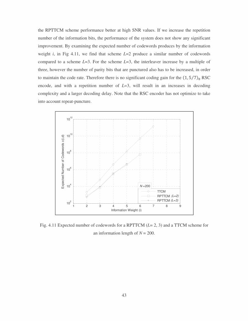
the RPTTCM scheme performance better at high SNR values. If we increase the repetition
number of the information bits, the performance of the system does not show any significant
improvement. By examining the expected number of codewords produces by the information
weight i, in Fig 4.11, we find that scheme L=2 produce a similar number of codewords
compared to a scheme L=3. For the scheme L=3, the interleaver increase by a multiple of
three, however the number of parity bits that are punctured also has to be increased, in order
to maintain the code rate. Therefore there is no significant coding gain for the ��� � �< RSC
encode, and with a repetition number of L=3, will result in an increases in decoding
complexity and a larger decoding delay. Note that the RSC encoder has not optimize to take
into account repeat-puncture.
Fig. 4.11 Expected number of codewords for a RPTTCM (L= 2, 3) and a TTCM scheme for
an information length of N = 200.
1 2 3 4 5 6 7 8 910
2
104
106
108
1010
1012
Information Weight (i)
Exp
ecte
d N
umbe
r of C
odew
ords
c(i,
d)
TTCMRPTTCM RPTTCM
N =200
(L=2)(L=3)
44
Fig. 4.12 Performance bound and simulation result for a RPTTCM and TTCM scheme for an information size N = 200 in a Rayleigh flat fading channel.
4 6 8 10 12 14 16
10-7
10-6
10-5
10-4
10-3
10-2
10-1
Eb/No (dB)
BE
R
Simulation Result,TTCMSimulation Result, RPTTCMPerformance Bound, TTCMPerformance Bound,RPTTCM
N =200
45
Chapter 5: Turbo Trellis-Coded Modulation and Repeat-Punctured Turbo
Trellis Coded Modulation
The fundamentals of Turbo codes and Trellis-Coded Modulation (TCM) schemes were
discussed in Chapter 3. The combination of both schemes results in a high performance code
for a bandwidth limited channel. The performance of the two systems was discussed in
Chapter 4.
5.1 Turbo Trellis-Coded Modulation
TCM scheme proposed by Ungerboek in 1982 [22], has been used in a variety of application
such telephone, satellite and microwave to name a few. Turbo codes (TC) achieve remarkable
performance at low SNR values, however they are not suitable for bandwidth limited
communication system. To achieve large coding gain and high bandwidth efficiency, the
combination of turbo codes with TCM schemes has been proposed in [6, 10, 17, 18, 25].
5.1.1 Encoder Structure
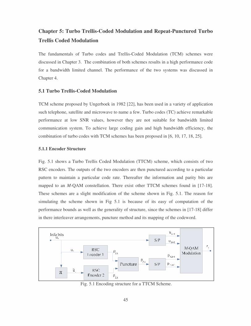
Fig. 5.1 shows a Turbo Trellis Coded Modulation (TTCM) scheme, which consists of two
RSC encoders. The outputs of the two encoders are then punctured according to a particular
pattern to maintain a particular code rate. Thereafter the information and parity bits are
mapped to an M-QAM constellation. There exist other TTCM schemes found in [17-18].
These schemes are a slight modification of the scheme shown in Fig. 5.1. The reason for
simulating the scheme shown in Fig 5.1 is because of its easy of computation of the
performance bounds as well as the generality of structure, since the schemes in [17-18] differ
in there interleaver arrangements, puncture method and its mapping of the codeword.
Fig. 5.1 Encoding structure for a TTCM Scheme.
46
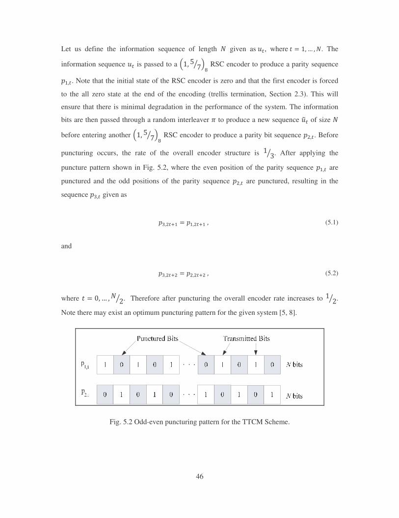
Let us define the information sequence of length � given as���, where�, � ��@ � �. The
information sequence �� is passed to a r�� � �³ s RSC encoder to produce a parity sequence
�.��. Note that the initial state of the RSC encoder is zero and that the first encoder is forced
to the all zero state at the end of the encoding (trellis termination, Section 2.3). This will
ensure that there is minimal degradation in the performance of the system. The information
bits are then passed through a random interleaver ? to produce a new sequence �B� of size �
before entering another r�� � �³ s RSC encoder to produce a parity bit sequence �!��. Before
puncturing occurs, the rate of the overall encoder structure is � �³ . After applying the
puncture pattern shown in Fig. 5.2, where the even position of the parity sequence �.�� are
punctured and the odd positions of the parity sequence �!�� are punctured, resulting in the
sequence ���� given as
���!�]. � �.�!�].�� (5.1)
and
���!�]! � �!�!�]!�� (5.2)
where , � ��@ �� �³ . Therefore after puncturing the overall encoder rate increases to � �³ .
Note there may exist an optimum puncturing pattern for the given system [5, 8].
Fig. 5.2 Odd-even puncturing pattern for the TTCM Scheme.
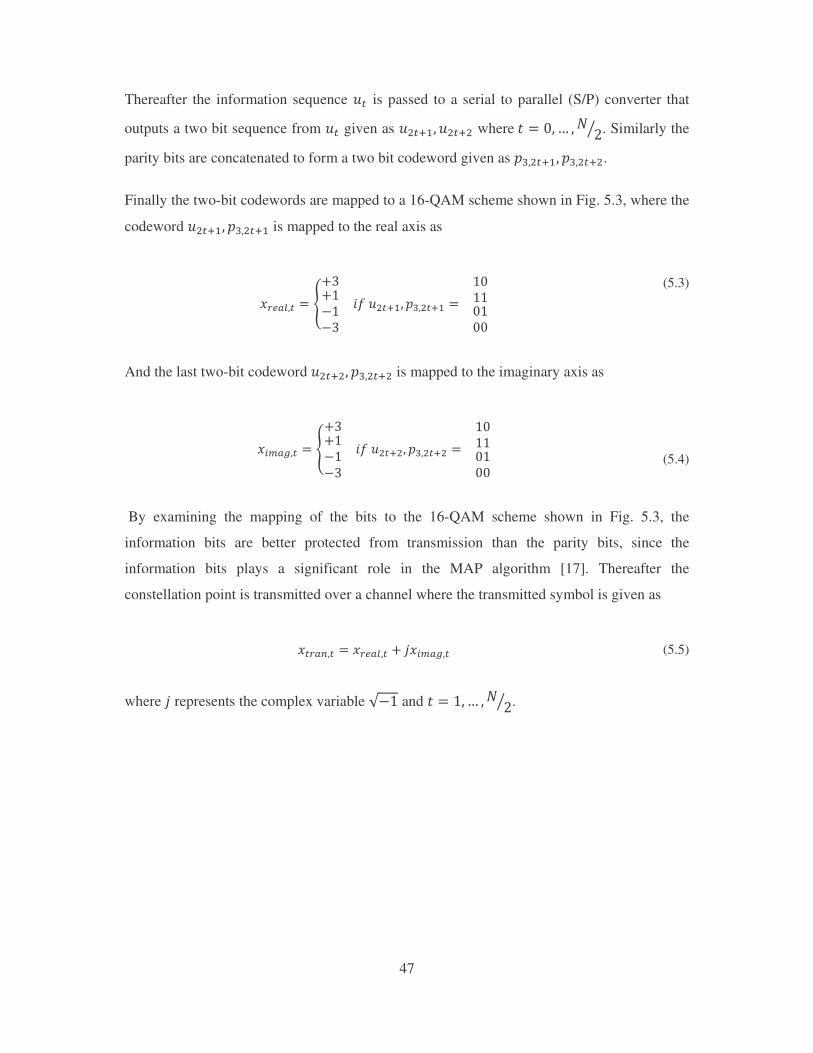
47
Thereafter the information sequence �� is passed to a serial to parallel (S/P) converter that
outputs a two bit sequence from �� given as �!�].� �!�]! where�, � ��@ � � �³ . Similarly the
parity bits are concatenated to form a two bit codeword given as ���!�].� ���!�]!.
Finally the two-bit codewords are mapped to a 16-QAM scheme shown in Fig. 5.3, where the
codeword �!�].� ���!�]. is mapped to the real axis as
:±(´`�� � µ;�;�\�\� �/��!�].� ���!�]. � ��������z (5.3)
And the last two-bit codeword �!�]!� ���!�]! is mapped to the imaginary axis as
: ¶ ´·�� � µ;�;�\�\� �/��!�]!� ���!�]! � ��������z
(5.4)
By examining the mapping of the bits to the 16-QAM scheme shown in Fig. 5.3, the
information bits are better protected from transmission than the parity bits, since the
information bits plays a significant role in the MAP algorithm [17]. Thereafter the
constellation point is transmitted over a channel where the transmitted symbol is given as
:�±´t�� � :±(´`�� ; -: ¶ ´·�� (5.5)
where - represents the complex variable W\� and , � ��@ � � �³ .
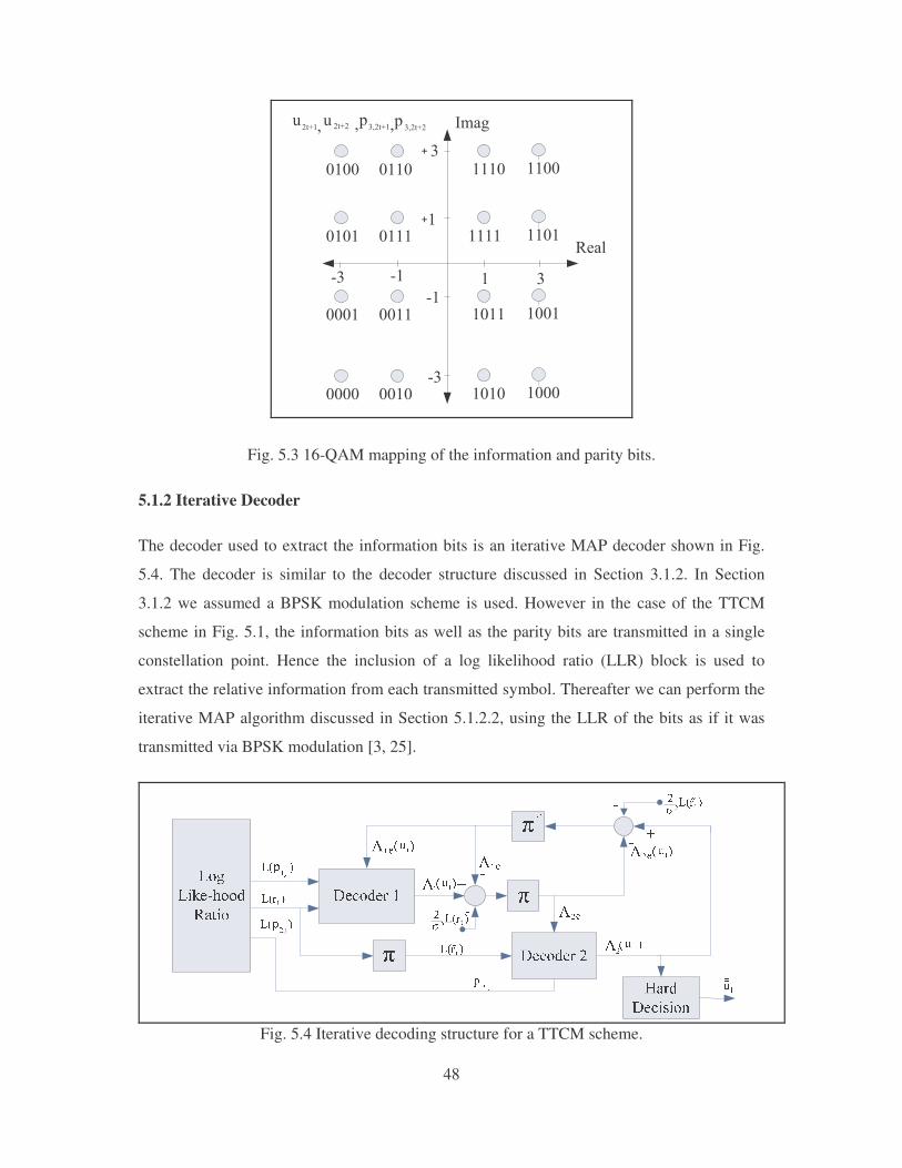
48
+�++ +��+ ���+ ��++
+�+� +��� ���� ��+�
+++� ++�� �+�� �++�
++++ ++�+ �+�+ �+++
)#) �#�
)
#)
�
#�
����
)����
����)����
� � � ,-�.
���'
�
�
Fig. 5.3 16-QAM mapping of the information and parity bits.
5.1.2 Iterative Decoder
The decoder used to extract the information bits is an iterative MAP decoder shown in Fig.
5.4. The decoder is similar to the decoder structure discussed in Section 3.1.2. In Section
3.1.2 we assumed a BPSK modulation scheme is used. However in the case of the TTCM
scheme in Fig. 5.1, the information bits as well as the parity bits are transmitted in a single
constellation point. Hence the inclusion of a log likelihood ratio (LLR) block is used to
extract the relative information from each transmitted symbol. Thereafter we can perform the
iterative MAP algorithm discussed in Section 5.1.2.2, using the LLR of the bits as if it was
transmitted via BPSK modulation [3, 25].
Fig. 5.4 Iterative decoding structure for a TTCM scheme.
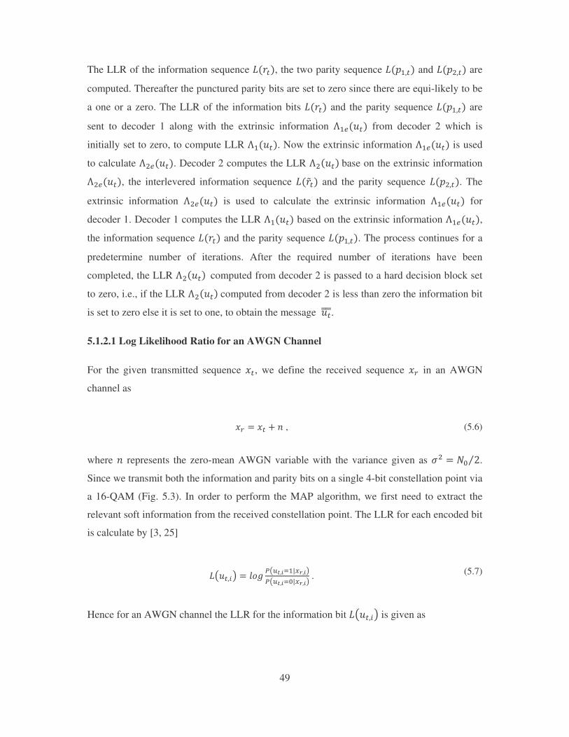
49
The LLR of the information sequence G�C�, the two parity sequence G��.�� and G��!�� are
computed. Thereafter the punctured parity bits are set to zero since there are equi-likely to be
a one or a zero. The LLR of the information bits G�C� and the parity sequence G��.�� are
sent to decoder 1 along with the extrinsic information D.(��� from decoder 2 which is
initially set to zero, to compute LLR D.���. Now the extrinsic information D.(��� is used
to calculate D!(���. Decoder 2 computes the LLR D!����base on the extrinsic information D!(���, the interlevered information sequence G�CE� and the parity sequence G��!��. The
extrinsic information D!(��� is used to calculate the extrinsic information D.(��� for
decoder 1. Decoder 1 computes the LLR D.��� based on the extrinsic information D.(���, the information sequence G�C� and the parity sequence G��.��. The process continues for a
predetermine number of iterations. After the required number of iterations have been
completed, the LLR D!�����computed from decoder 2 is passed to a hard decision block set
to zero, i.e., if the LLR D!����computed from decoder 2 is less than zero the information bit
is set to zero else it is set to one, to obtain the message ��FFF. 5.1.2.1 Log Likelihood Ratio for an AWGN Channel
For the given transmitted sequence :�, we define the received sequence :± in an AWGN
channel as
:± � :� ; � , (5.6)
where � represents the zero-mean AWGN variable with the variance given as ! � �� �< .
Since we transmit both the information and parity bits on a single 4-bit constellation point via
a 16-QAM (Fig. 5.3). In order to perform the MAP algorithm, we first need to extract the
relevant soft information from the received constellation point. The LLR for each encoded bit
is calculate by [3, 25]
GT��� U � $HI �T¸Y�Zi.K¹º�ZU�T¸Y�Zi�K¹º�ZU . (5.7)
Hence for an AWGN channel the LLR for the information bit GT��� U is given as
50
GT��� U � »¼ h $HIg (¹½J� d3¾3r¹º�Z�¼� s3L¿�ZÀÁY�ZÂdg (¹½J� d3¾3r¹º�Z�¼� s3L¿�ZÀÁY�ZÂf ,
(5.8)
where »¼ is a constant and ��� is the set of all constellation points for �x��� @ ��©�. However
the LLR for all encoded bits is not strictly Gaussian. Thus the binary turbo decoder is no
longer optimal for the coded modulation scheme. However, simulation results indicate for
large SNR value, the LLR of the encoded bits is close to a Gaussian random variable with
variance ! if we set »¼ � [3! [3, 25] .
After computing LLR rGT��� U� GT�.� U������GT�!� Us for each of the bits in the received
constellation point :±� , we can then use the iterative MAP decoder in Section 3.1.2, where
we treat LLR values as if they were transmitted via a BPSK medium [3, 25]. Note that the
value of the LLR of the puncture parity bit is set to zero since it is equi-likely to be a one or a
zero.
5.1.2.2 Log Likelihood Ratio for a Rayleigh Fading Channel
The decoder for a Rayleigh flat fading channel is similar to that of an AWGN channel. For
the Rayleigh channel we assume that the channel state information (CSI) is known at the
receiver and for the given transmitted sequence :�, we define the received sequence :± as
:± � %:� ; � , (5.9)
where % represents the fading co-efficient. Similarly to the AWGN channel we first need to
compute LLR of the encoded bits. Therefore to calculate LLR in a Rayleigh flat fading
channel with the CSI known at the receiver we need to compute,
GT��� U � $HI �T¸Y�Zi.K¹º�Z�ÃZU�T¸Y�Zi�K¹º�Z�ÃZU . (5.10)
The LLR for the information bit GT��� U is given as
51
GT��� U � »¼ g (¹½J� d3¾3r¹º�Z�ÃZ¼� s3L¿�ZÀÁY�ZÂdg (¹½J� d3¾3r¹º�Z�ÃZ¼� s3L¿�ZÀÁY�ZÂf ,
(5.11)
where »¼ is a constant. After computing LLR rGT��� U� GT�.� U������GT�!� Us for each of the
bits in the received constellation point :±� , we can then use the iterative MAP algorithm in
Section 3.1.2.1, where we treat LLR values as if they was transmitted via a BPSK medium.
5.1.3 Simulation Results
Fig. 5.5 shows the simulation results for 2bits/sec/Hz TTCM scheme presented in Fig. 5.1 for
a zero-mean AWGN channel with the variance given as ! � �� �< . We simulated for an
information size of � � ��� and � � ��� respectively. The decoder computes 18 iterations
before making a decision on the decoded bits. The simulations were terminated after 80
frame errors were detected for each SNR value. The bit error rate (BER) of ���� occurs at a
SNR of 6 dB for �=800 and a BER of ���� occurs at a SNR of 8.94 dB for �=200. As
expected the scheme performs better for the larger information size of �=800, which results
in an interleaver gain of 2.94 dB.
Fig. 5.6 shows the simulation results for 2 bits/sec/Hz TTCM scheme presented in Fig. 5.1
for a Rayleigh flat fading channel with the CSI known at the receiver. We simulated for an
information size of �=800 and �=200. The decoder computes 18 iterations before making a
hard decision on the decoded bits. The simulations were terminated after 80 frame errors
were detected for each SNR value. The BER of ���� occurs at a SNR of 10.8 dB for �=800
and a BER of ���6 occurs at a SNR of 14 dB for �=200. As expected the scheme performs
better for the larger information size of �=800, which is the result of the interleaver gain.
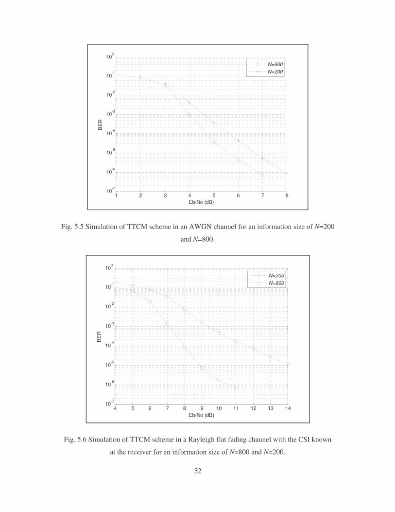
52
Fig. 5.5 Simulation of TTCM scheme in an AWGN channel for an information size of N=200
and N=800.
Fig. 5.6 Simulation of TTCM scheme in a Rayleigh flat fading channel with the CSI known
at the receiver for an information size of N=800 and N=200.
1 2 3 4 5 6 7 810
-7
10-6
10-5
10-4
10-3
10-2
10-1
100
Eb/No (dB)
BE
R
N=800N=200
4 5 6 7 8 9 10 11 12 13 1410
-7
10-6
10-5
10-4
10-3
10-2
10-1
100
Eb/No (dB)
BE
R
N=200N=800
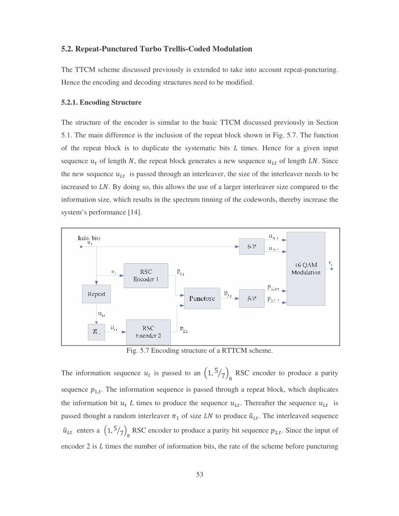
53
5.2. Repeat-Punctured Turbo Trellis-Coded Modulation
The TTCM scheme discussed previously is extended to take into account repeat-puncturing.
Hence the encoding and decoding structures need to be modified.
5.2.1. Encoding Structure
The structure of the encoder is simular to the basic TTCM discussed previously in Section
5.1. The main difference is the inclusion of the repeat block shown in Fig. 5.7. The function
of the repeat block is to duplicate the systematic bits G times. Hence for a given input
sequence �� of length �, the repeat block generates a new sequence �°� of length G�. Since
the new sequence �°� is passed through an interleaver, the size of the interleaver needs to be
increased to G�. By doing so, this allows the use of a larger interleaver size compared to the
information size, which results in the spectrum tinning of the codewords, thereby increase the
system’s performance [14].
Fig. 5.7 Encoding structure of a RTTCM scheme.
The information sequence �� is passed to an r�� � �³ s RSC encoder to produce a parity
sequence �.��. The information sequence is passed through a repeat block, which duplicates
the information bit �� L times to produce the sequence �°�. Thereafter the sequence �°� is
passed thought a random interleaver ?. of size G� to produce��B°�. The interleaved sequence ��B°� enters a r�� � �³ s RSC encoder to produce a parity bit sequence �!��. Since the input of
encoder 2 is G times the number of information bits, the rate of the scheme before puncturing
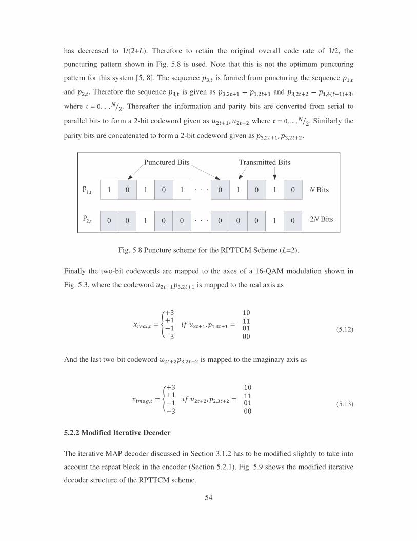
54
has decreased to 1/(2+L). Therefore to retain the original overall code rate of 1/2, the
puncturing pattern shown in Fig. 5.8 is used. Note that this is not the optimum puncturing
pattern for this system [5, 8]. The sequence ���� is formed from puncturing the sequence �.�� and �!��� Therefore the sequence ���� is given as ���!�]. � �.�!�]. and ���!�]! � �.�7���.]�,
where , � ��@ � � �³ . Thereafter the information and parity bits are converted from serial to
parallel bits to form a 2-bit codeword given as �!�].� �!�]! where , � ��@ �� �³ . Similarly the
parity bits are concatenated to form a 2-bit codeword given as����!�].� ���!�]!.
� + � + � + ��������
+ � + � + � +�������
+ � +
+ �
������������ /����-�������
��
��
+ + +� +
�����
�������+
Fig. 5.8 Puncture scheme for the RPTTCM Scheme (L=2).
Finally the two-bit codewords are mapped to the axes of a 16-QAM modulation shown in
Fig. 5.3, where the codeword �!�].���!�]. is mapped to the real axis as
:±(´`�� � µ;�;�\�\� �/��!�].� �.���]. � ��������z
(5.12)
And the last two-bit codeword �!�]!���!�]! is mapped to the imaginary axis as
: ¶ ´·�� � µ;�;�\�\� �/��!�]!� �!���]! � ��������z
(5.13)
5.2.2 Modified Iterative Decoder
The iterative MAP decoder discussed in Section 3.1.2 has to be modified slightly to take into
account the repeat block in the encoder (Section 5.2.1). Fig. 5.9 shows the modified iterative
decoder structure of the RPTTCM scheme.

55
&��
�'�.��0-
&��
�'�.��0-
��
�����
��������
�1
��
��.
�����
2
�����
2
��. �
�
�
�
� 2 3
���2 3
���2 3
2�.�
2�1�#0����
����
�
�2 32�2 32��! �
� �
�
� �
� �� �
��
� ���
��
��" 2 32��!
2 3��
�"
��
��
�
�
##
Fig. 5.9 Iterative decoding structure for a RPTTCM scheme.
Since the message is transmitted via 16-QAM modulation, the individual bits must be
extracted from the incoming symbol using the LLR (discussed in Section 5.1.2.1 for the
AWGN channel and Section 5.1.2.2 for a Rayleigh flat fading channel). Thereafter the
punctured parity bits are set to zero since they are equi-likely to be a one or a zero. The
information bits G���, the parity bits GT�.��U, and the extrinsic information D.(��� which is
initially set to zero, are sent to decoder 1 to compute LLR D.���. The extrinsic information
extracted from decoder 1, D.(���� needs to be passed on to decoder 2. However decoder 2
requires G� extrinsic information for G� information bits. Therefore the extrinsic
information from decoder 1, �D.(��� and the LLR of the information bits G��� are repeated
to form the sequence G�GC.�� and interleaved, G�GCE.��, before they are passed through to
decoder 2, along with the parity sequence�GT�!��U. Decoder 2 computes the LLR D!��� of
the information bits to complete the first iteration of the decoder. For the next iteration the
extrinsic information D!(����from decoder 2 needs to be passed to decoder 1. Yet again
decoder 2 computes G� number of extrinsic information bits. Therefore before it is passed to
decoder 1, the extrinsic information from decoder 2 is first deinterleaved and then averaged
over G bits. Decoder 1 then computes the LLR of the information bits, and the process
continues for a predetermined number of iterations. The performance of the system improves
as the number of iterations is increased. After the required number of iterations has been
completed, the LLR computed from decoder 2 is deinterleaved. The average over L bits is
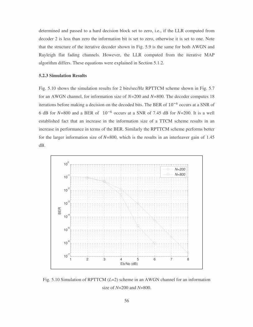
56
determined and passed to a hard decision block set to zero, i.e., if the LLR computed from
decoder 2 is less than zero the information bit is set to zero, otherwise it is set to one. Note
that the structure of the iterative decoder shown in Fig. 5.9 is the same for both AWGN and
Rayleigh flat fading channels. However, the LLR computed from the iterative MAP
algorithm differs. These equations were explained in Section 5.1.2.
5.2.3 Simulation Results
Fig. 5.10 shows the simulation results for 2 bits/sec/Hz RPTTCM scheme shown in Fig. 5.7
for an AWGN channel, for information size of �=200 and �=800. The decoder computes 18
iterations before making a decision on the decoded bits. The BER of ���� occurs at a SNR of
6 dB for �=800 and a BER of ���� occurs at a SNR of 7.45 dB for �=200. It is a well
established fact that an increase in the information size of a TTCM scheme results in an
increase in performance in terms of the BER. Similarly the RPTTCM scheme performs better
for the larger information size of��=800, which is the results in an interleaver gain of 1.45
dB.
Fig. 5.10 Simulation of RPTTCM (L=2) scheme in an AWGN channel for an information
size of N=200 and N=800.
1 2 3 4 5 6 7 810
-7
10-6
10-5
10-4
10-3
10-2
10-1
100
Eb/No (dB)
BE
R
N=200N=800
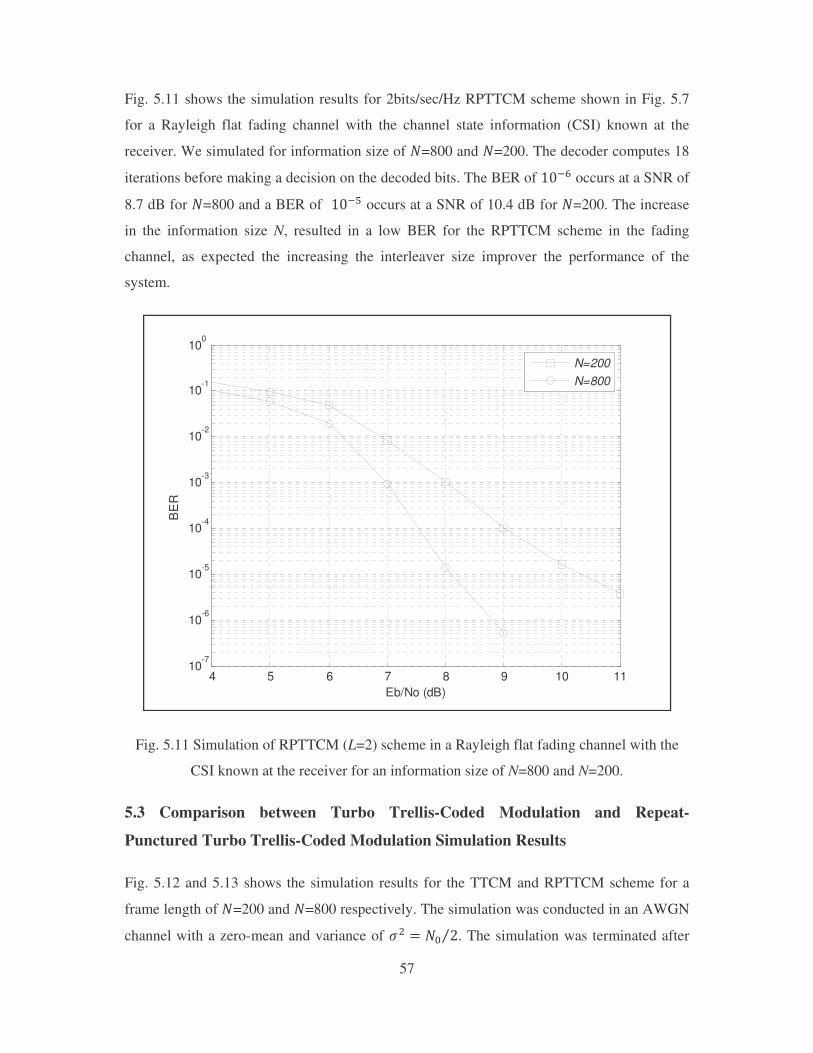
57
Fig. 5.11 shows the simulation results for 2bits/sec/Hz RPTTCM scheme shown in Fig. 5.7
for a Rayleigh flat fading channel with the channel state information (CSI) known at the
receiver. We simulated for information size of �=800 and �=200. The decoder computes 18
iterations before making a decision on the decoded bits. The BER of ���� occurs at a SNR of
8.7 dB for �=800 and a BER of ���6 occurs at a SNR of 10.4 dB for �=200. The increase
in the information size N, resulted in a low BER for the RPTTCM scheme in the fading
channel, as expected the increasing the interleaver size improver the performance of the
system.
Fig. 5.11 Simulation of RPTTCM (L=2) scheme in a Rayleigh flat fading channel with the
CSI known at the receiver for an information size of N=800 and N=200.
5.3 Comparison between Turbo Trellis-Coded Modulation and Repeat-
Punctured Turbo Trellis-Coded Modulation Simulation Results
Fig. 5.12 and 5.13 shows the simulation results for the TTCM and RPTTCM scheme for a
frame length of �=200 and �=800 respectively. The simulation was conducted in an AWGN
channel with a zero-mean and variance of ! � �� �< . The simulation was terminated after
4 5 6 7 8 9 10 1110
-7
10-6
10-5
10-4
10-3
10-2
10-1
100
Eb/No (dB)
BE
R
N=200N=800
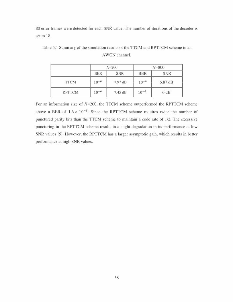
58
80 error frames were detected for each SNR value. The number of iterations of the decoder is
set to 18.
Table 5.1 Summary of the simulation results of the TTCM and RPTTCM scheme in an
AWGN channel.
N=200 N=800 BER SNR BER SNR
TTCM ���� 7.97 dB ���� 6.87 dB
RPTTCM ���� 7.45 dB ���� 6 dB
For an information size of �=200, the TTCM scheme outperformed the RPTTCM scheme
above a BER of ��© ª ���6. Since the RPTTCM scheme requires twice the number of
punctured parity bits than the TTCM scheme to maintain a code rate of 1/2. The excessive
puncturing in the RPTTCM scheme results in a slight degradation in its performance at low
SNR values [5]. However, the RPTTCM has a larger asymptotic gain, which results in better
performance at high SNR values.
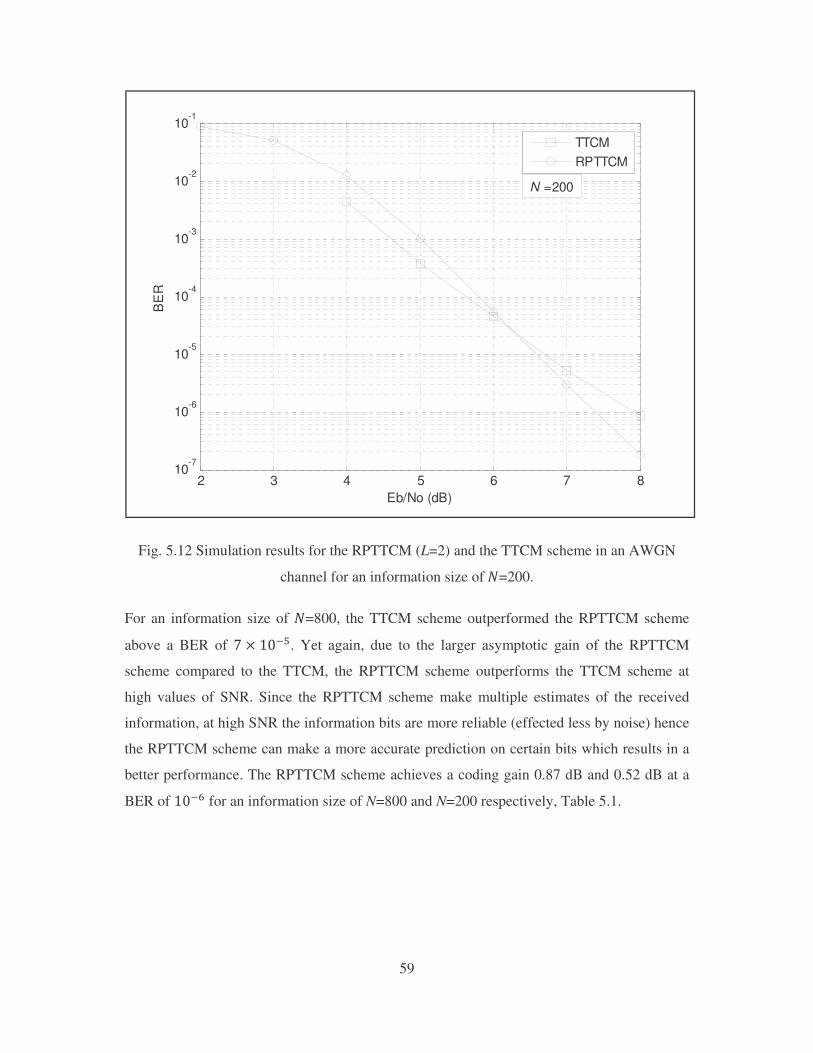
59
Fig. 5.12 Simulation results for the RPTTCM (L=2) and the TTCM scheme in an AWGN
channel for an information size of��=200.
For an information size of �=800, the TTCM scheme outperformed the RPTTCM scheme
above a BER of � ª ���6. Yet again, due to the larger asymptotic gain of the RPTTCM
scheme compared to the TTCM, the RPTTCM scheme outperforms the TTCM scheme at
high values of SNR. Since the RPTTCM scheme make multiple estimates of the received
information, at high SNR the information bits are more reliable (effected less by noise) hence
the RPTTCM scheme can make a more accurate prediction on certain bits which results in a
better performance. The RPTTCM scheme achieves a coding gain 0.87 dB and 0.52 dB at a
BER of ���� for an information size of N=800 and N=200 respectively, Table 5.1.
2 3 4 5 6 7 810
-7
10-6
10-5
10-4
10-3
10-2
10-1
Eb/No (dB)
BE
R
TTCMRPTTCM
N =200
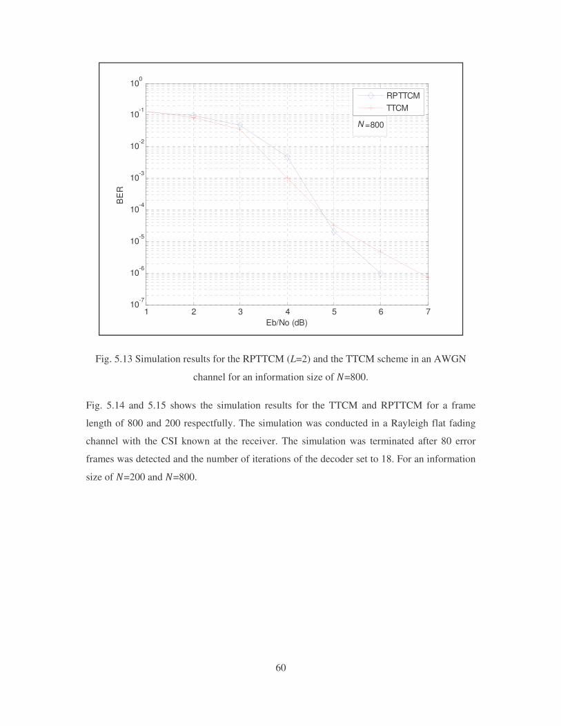
60
Fig. 5.13 Simulation results for the RPTTCM (L=2) and the TTCM scheme in an AWGN
channel for an information size of �=800.
Fig. 5.14 and 5.15 shows the simulation results for the TTCM and RPTTCM for a frame
length of 800 and 200 respectfully. The simulation was conducted in a Rayleigh flat fading
channel with the CSI known at the receiver. The simulation was terminated after 80 error
frames was detected and the number of iterations of the decoder set to 18. For an information
size of �=200 and �=800.
1 2 3 4 5 6 710
-7
10-6
10-5
10-4
10-3
10-2
10-1
100
Eb/No (dB)
BE
R
RPTTCMTTCM
N =800
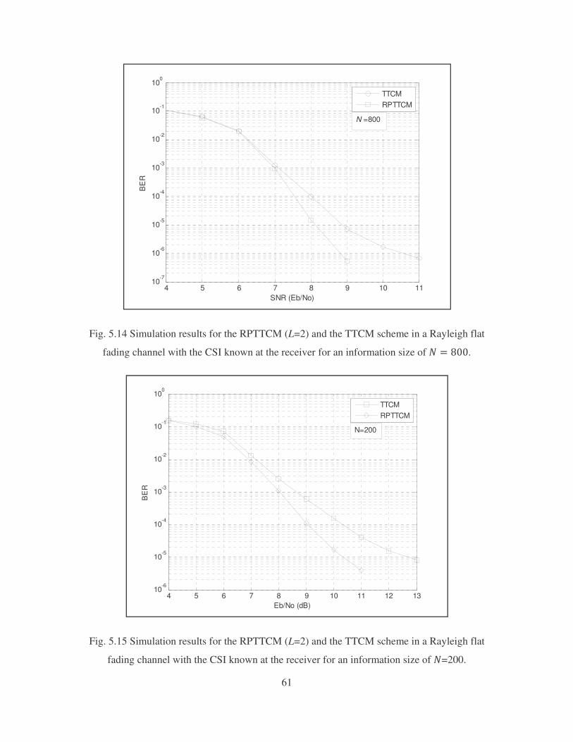
61
Fig. 5.14 Simulation results for the RPTTCM (L=2) and the TTCM scheme in a Rayleigh flat
fading channel with the CSI known at the receiver for an information size of � � ���.
Fig. 5.15 Simulation results for the RPTTCM (L=2) and the TTCM scheme in a Rayleigh flat
fading channel with the CSI known at the receiver for an information size of �=200.
4 5 6 7 8 9 10 1110
-7
10-6
10-5
10-4
10-3
10-2
10-1
100
SNR (Eb/No)
BE
R
TTCMRPTTCM
N =800
4 5 6 7 8 9 10 11 12 1310
-6
10-5
10-4
10-3
10-2
10-1
100
Eb/No (dB)
BE
R
TTCMRPTTCM
N=200
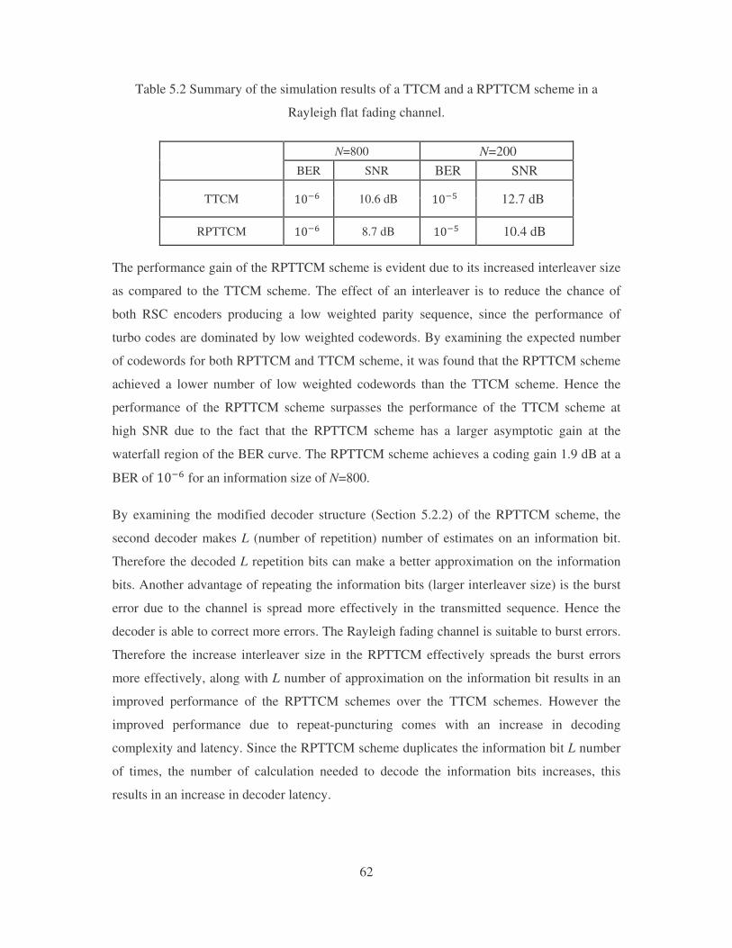
62
Table 5.2 Summary of the simulation results of a TTCM and a RPTTCM scheme in a
Rayleigh flat fading channel.
N=800 N=200 BER SNR BER SNR
TTCM ���� 10.6 dB ���6 12.7 dB
RPTTCM ���� 8.7 dB ���6 10.4 dB
The performance gain of the RPTTCM scheme is evident due to its increased interleaver size
as compared to the TTCM scheme. The effect of an interleaver is to reduce the chance of
both RSC encoders producing a low weighted parity sequence, since the performance of
turbo codes are dominated by low weighted codewords. By examining the expected number
of codewords for both RPTTCM and TTCM scheme, it was found that the RPTTCM scheme
achieved a lower number of low weighted codewords than the TTCM scheme. Hence the
performance of the RPTTCM scheme surpasses the performance of the TTCM scheme at
high SNR due to the fact that the RPTTCM scheme has a larger asymptotic gain at the
waterfall region of the BER curve. The RPTTCM scheme achieves a coding gain 1.9 dB at a
BER of ���� for an information size of N=800.
By examining the modified decoder structure (Section 5.2.2) of the RPTTCM scheme, the
second decoder makes L (number of repetition) number of estimates on an information bit.
Therefore the decoded L repetition bits can make a better approximation on the information
bits. Another advantage of repeating the information bits (larger interleaver size) is the burst
error due to the channel is spread more effectively in the transmitted sequence. Hence the
decoder is able to correct more errors. The Rayleigh fading channel is suitable to burst errors.
Therefore the increase interleaver size in the RPTTCM effectively spreads the burst errors
more effectively, along with L number of approximation on the information bit results in an
improved performance of the RPTTCM schemes over the TTCM schemes. However the
improved performance due to repeat-puncturing comes with an increase in decoding
complexity and latency. Since the RPTTCM scheme duplicates the information bit L number
of times, the number of calculation needed to decode the information bits increases, this
results in an increase in decoder latency.
63
Chapter 6: Conclusion and Future Research
6.1 Conclusion
A turbo trellis-coded modulation (TTCM) scheme that combines the performance of turbo
code with the bandwidth efficiency of trellis-coded modulation was discussed. The TTCM
scheme was extended to include repeat-puncturing, known as repeat-punctured turbo trellis-
coded modulation (RPTTCM). The repetition of information bits allows the use of a larger
interleaver size than that of the information size. Thereafter the encoded bits are punctured to
maintain the code rate. The puncturing of the turbo code results in the degradation in the
performance, however the coding gain due to a larger interleaver size surpasses the
degradation in performance due to puncturing. The modifications needed for the TTCM
scheme at the encoder as well as the decoder to take into account repeat-puncturing were
discussed.
The RPTTCM and the TTCM scheme were simulated in an AWGN channel. A summary of
the simulation results for the TTCM and RPTTCM scheme is shown in Table 5.1. The results
for the RPTTCM scheme were compared with the TTCM scheme. For an information size of � � ���, the TTCM scheme outperformed the RPTTCM scheme above a BER of ��© ª���6. The RPTTCM scheme has a larger asymptotic gain which results in a steeper gradient
in the waterfall region of the BER curve, resulting in a better performance below a BER of ��© ª ���6. For an information size of �=800, the TTCM scheme outperformed the
RPTTCM scheme above a BER of � ª ���6. For a large information size (�=800) the
degradation due to puncturing is surpassed by the coding gain due to the interleaver. The
RPTTCM scheme achieved a coding gain of approximately 0.87 dB at a BER of ����, since
performances of turbo code are dominated by low weighted codewords. By examining the
expected number of codewords for the RPTTCM and the TTCM schemes, it was found that
the RPTTCM scheme produces less number of low weighted codewords than with the TTCM
scheme. Which contributes to the increase in performance of the RPTTCM scheme.
Both the RPTTCM and the TTCM schemes were simulated in a Rayleigh flat fading channel
with the channel state information (CSI) known at the receiver. A summary of the simulation
results for the TTCM and RPTTCM scheme is shown in Table 5.2. The results for the
RPTTCM scheme were compared with the TTCM scheme. For an information size of �=800
64
and �=200, the RPTTCM scheme has a coding gain of 1.9 dB at a BER of ����. The effect
of increasing the interleaver size in the RPTTCM scheme allows burst errors to be distributed
efficiently to allow the decoder to correct more errors. Along with the decoder’s ability to
make L (number for repetition of the information bits) number of estimates on the
information bits compared to the TTCM scheme, this results in an increase in performance
for the RPTTCM scheme. However, the improved performance due to repeat-puncturing
comes with an increase in decoding complexity and latency.
Finally the performance bound of the BER was derived for the TTCM and RPTTCM
schemes. The derivation of the performance bound for the TTCM scheme followed closely
the derivation for both an AWGN channel proposed by [25] and a Rayleigh flat fading
channel [11]. The theoretical bound matched the simulation results at high SNR values for an
AWGN and a Rayleigh flat fading channel. The performance bound of the bit error rate of a
TTCM scheme was extended to the RPTTCM scheme for both channels. The simulation
result converges towards the theoretical bound for the RPTTCM scheme in an AWGN
channel as well as the Rayleigh flat fading channel.
6.2 Future Research
There are various parts of the RPTTCM scheme that can be optimised to improve the
performance of the scheme. The work carried out in this dissertation can be extended to
• Investigate the use of different interleaver design, the use of S-random and code-
matching interleaver.
• Develop an optimal puncturing scheme that reduces the degradation in performance
of the code.
• The use of different component code can also be investigated, the use of the generator
polynomial, constrain length of the RSC encoder.
• Investigate the performance of RPTTCM in a Nakagami channel.
• The use of dual repeat-puncture can be investigated on TTCM schemes.
• The use of repeat-puncturing can be investigated on different concatenated schemes
namely the serial concatenated schemes.
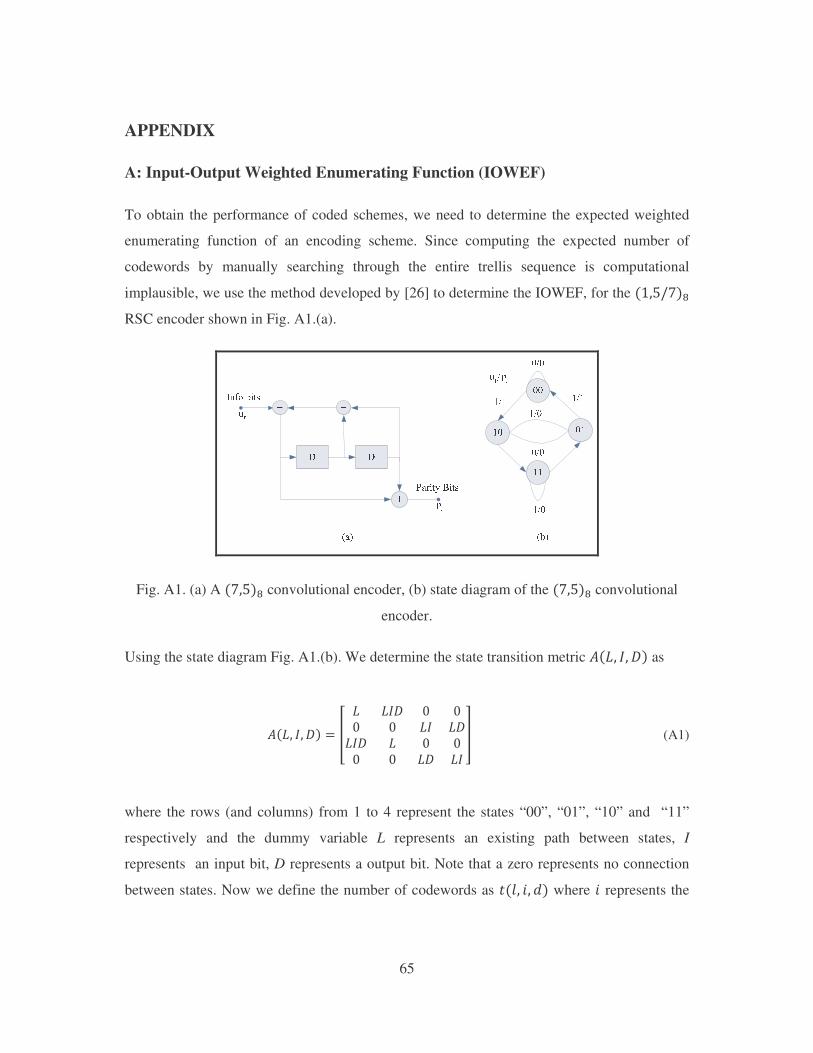
65
APPENDIX
A: Input-Output Weighted Enumerating Function (IOWEF)
To obtain the performance of coded schemes, we need to determine the expected weighted
enumerating function of an encoding scheme. Since computing the expected number of
codewords by manually searching through the entire trellis sequence is computational
implausible, we use the method developed by [26] to determine the IOWEF, for the ������
RSC encoder shown in Fig. A1.(a).
Fig. A1. (a) A ���� convolutional encoder, (b) state diagram of the ���� convolutional
encoder.
Using the state diagram Fig. A1.(b). We determine the state transition metric �G� �� 4 as
Ä�G� �� 4 � Å G G�4 � �� � G� G4G�4 G � �� � G4 G� Æ (A1)
where the rows (and columns) from 1 to 4 represent the states “00”, “01”, “10” and “11”
respectively and the dummy variable L represents an existing path between states, I
represents an input bit, D represents a output bit. Note that a zero represents no connection
between states. Now we define the number of codewords as ,�$� �� 2 where � represents the
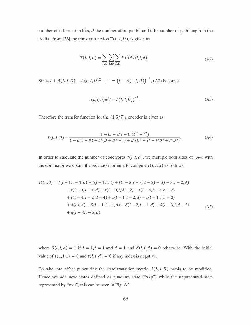
66
number of information bits, 2 the number of output bit and�$ the number of path length in the
trellis. From [26] the transfer function�§�G� �� 4, is given as
§�G� �� 4 �^^^G`� 4¥,�$� �� 2�¥V� V�`V� (A2)
Since � ; Ä�G� �� 4 ; Ä�G� �� 4! ;Ç � T� \ Ä�G� �� 4U�., (A2) becomes
T�G� �� 4=T� \ �G� �� 4U�.� (A3)
Therefore the transfer function for the ������ encoder is given as
§�G� �� 4 � � \ G� \ G!� \ G��4! ; �!� \ G�� ; 4 ; G��4 ; 4! \ � ; G7�4! \ �! \ �!47 ; �74!� (A4)
In order to calculate the number of codewords ,�$� �� 2, we multiple both sides of (A4) with
the dominator we obtain the recursion formula to compute ,�$� �� 2 as follows
,�$� �� 2 � ,�$ \ �� � \ �� 2 ; ,�$ \ �� �� 2 ; ,�$ \ �� � \ �� 2 \ � \ ,�$ \ �� � \ �� 2\ ,�$ \ �� � \ �� 2 ; ,�$ \ �� �� 2 \ � \ ,�$ \ ¨� � \ ¨� 2 \ �; ,�$ \ ¨� � \ �� 2 \ ¨ ; ,�$ \ ¨� � \ �� 2 \ ,�$ \ ¨� �� 2 \ �; È�$� �� 2 \ È�$ \ �� � \ �� 2 \ È�$ \ �� � \ �� 2 \ È�$ \ �� �� 2 \ �; È�$ \ �� � \ �� 2 (A5)
where �$� �� 2 � � if $ � �� � � ������2 � � and �$� �� 2 � � otherwise. With the initial
value of ,������ � � and ,�$� �� 2 � � if any index is negative.�To take into effect puncturing the state transition metric �G� �� 4 needs to be modified.
Hence we add new states defined as puncture state (“xxp”) while the unpunctured state
represented by “xxu”, this can be seen in Fig. A2.
67
Fig. A2 Modified trellis diagram taking into account the punctured states.
Hence the state transition metric �G� �� 4 becomes
Ä�G� �� 4 �ÉÊÊÊÊÊÊË � G � G�4 � � � �G � G� � � � � G4� � � � � G� � �� � � � G� � G �� G�4 � G � � � �G� � G � � � � �� � � � � G4 � G�� � � � G � G� � ÌÍÍ
ÍÍÍÍÎ�� (A6)
where the rows (and columns) from 1 to 8 represents the states “00u”, “00p”, “01u”, “01p”,
“10u”, “10p”, “11u” and “11p” respectively. By following the method above, the recursion
formula used to compute ,�$� �� 2 can be determined.
68
References
[1] C. E. Shannon, “A Mathematical Theory of Communication”, BSTJ, vol. 27, pp 379-
423 (Part one), pp. 623 - 656 (Part two), Oct. 1948.
[2] C. Berrou, A. Glavieux and P. Thitimajshima, “Near Shannon limit error-correcting
coding and decoding: Turbo-codes”, in Proc. of IEEE. International Conference on
Communication (ICC), vol. 3, May 1993.
[3] B. Vucetic and J Yuan, “Turbo Codes Principles and Application”, Kluwer Academic
Publishers, 2000.
[4] D. Divsalar and F. Pollara, “Multiple Turbo Codes For Deep Space Communication”,
TDA Progress Report 24-12, pp. 66 - 77, Feb. 1995.
[5] H. Balta, L. Trifina and A. Rusinaru, “The Effect of Puncturing on the Convolutional
Turbo-Codes Performance”, Electronic and Telecommunications Faculty, University
Politehnica of Timisoara, 1997.
[6] S. Benedetto, D. Dizsalar, G. Montorsi and F. Pollara, “Parallel concatenated trellis
coded modulation”, Proc. of IEEE ICC’96, vol. 2, pp. 974 - 978, Mar. 1996.
[7] I. Chatzigeorgiou, M. R. D. Rodrigues, I. J. Wassell and R. Carrasco, "Punctured
binary turbo-codes with optimized performance", Proc. IEEE 62nd Vehicular Technology
Conference (VTC'05-Fall), Dallas, Texas, USA, Sept. 2005
[8] F. Mo, S. C. Kwatra and J. Kim, “Analysis of Puncturing Pattern for High Rate Turbo
Codes”, IEEE Military Communications Conference Proceedings, vol. 1, no. 1, pp. 547-550,
Aug. 2002.
[9] I. Chatzigeorgiou, M. R. D. Rodrigues, I.J. Wassell and R. Carrasco, “Pseudo-random
Puncturing: A technique to lower the error floor of turbo codes”, IEEE International
Symposium on Info. Theory, pp. 656-660, Jul. 2008.
[10] D. Divsalar and F. Pollara, “On the Design of Turbo Codes”, TDA Progress Report
42-123, pp. 99 - 121, Nov. 1995.
69
[11] T. M. Duman and M. Salehi, “Performance bound for Turbo-Coded Modulation
Systems over Fading channel”, IEEE Tran. on Comm., vol. 47, no. 10, pp. 1495 - 1501, Oct.
1999.
[12] N. Fajar and H. Ogiwara, “Performance evaluation method of Bit-Interleaved Turbo
Trellis- Coded Modulation and its Optimization”, IEICE Tran. Fund., vol. E87-A, no. 6, pp.
1583 - 1590, Jun. 2004.
[13] H. R. Sadjadpour, N. J. A. Sloane, M. Salehi, G. Nebe, “Interleaver Design for Turbo
Codes”, IEEE Journal on SAC, vol. 19, no. 2, pp. 831 - 837, May 2001.
[14] Y. Kim, J. Cho, W. Oh and K. Cheun, “Improving the performance of turbo codes by
repetition and puncturing”, Division of Electrical and Computer Engineering, Pohang
University of Science and Technology, 1996.
[15] J. M. Mouatcho Moualeu, H. Xu, and F. Takawira, “Cooperative diversity using repeat-punctured turbo codes,” Trans. SAIEE, vol. 100, no. 2, Jun. 2009. [16] P. Narushan, X HongJun and T. Fambirai, “Repeat-Puncture Superorthogonal
Convolutional Turbo Codes in AWGN and Flat Rayleigh Fading Channels”, Trans. SAIEE,
vol. 99, no. 2, Jun. 2009.
[17] P, Robertson and T. Wörz, “Bandwidth-Efficient Turbo Trellis –Coded Modulation
Usinf Punctured Component Codes”, IEEE JSA in Comms., vol. 16, no. 2, pp. 206 - 218, Feb.
1998.
[18] H. Ogiwara, A. Mizatane and K. Koike, “Performance evaluation of parallel
concatenated Trellis- Coded Modulation”, IEICE Tran. Fund., vol. E84-A, no. 10, pp. 2410 -
2417, Oct. 2001.
[19] S. Benedetto, Sergio and Montorsi, Guido, “Unveiling turbo-codes: some results on
parallel concatenated coding schemes”, IEEE Trans. on Info. Theory, vol. 42, no. 2, pp. 409 -
428, Mar. 1996.
[20] L. R. Bahl, J. Cocke, F. Jelinek, and J. Raviv, “Optimal decoding of linear codes for
minimizing symbol error rate”, IEEE Trans. Inform. Theory, vol. 20, no. 2, pp. 284 - 287,
Mar. 1979.
70
[21] C. Berrou, A. Glavieux, “Near optimum error correcting coding and decoding: Turbo-
codes”, IEEE Trans. Comms., vol. 44, no. 10, pp. 1261 - 1271, Oct. 1996.
[22] G. Ungerboeck, “Channel coding With Multilevel/phase signalling”, IEEE Tran.
Fund, Info. Theory, vol 25, no. 1, pp. 55 - 67, Jan. 1982.
[23] J. Hagenauer and P. Hoeher, “A Viterbi algorithm with soft-decision outputs and its
applications”, IEEE GLOBECOM’89, Dallas, TX, pp. 1680 - 1686, Nov. 1989.
[24] G. D. Forney, “The Viterbi algorithm,” Proc. IEEE, vol. 61, no. 3, pp. 218 - 278, Mar.
1973.
[25] T. M. Duman and M.Salehi, “Performance bound for Turbo-Coded Modulation
Systems”, IEEE Tran. Comms., vol. 47, pp. 511 - 521, Apr. 1999.
[26] D. Divsalar, S. Dolinar and F. Pollara, “Transfer Function Bound on the Performance
of Turbo-Code”, TDA Progress Report 42-122, pp. 44 - 55, Aug. 1995.
[27] D. Divsalar and M. K. Simon, “The design of trellis coded MPSK for fading channel:
Performance criteria”, IEEE Tran. Comms.,vol. 36, no. 9, pp. 1004 - 1012, Sept. 1988.
�
![Trellis-Coded Modulation [TCM] - Educypediaeducypedia.karadimov.info/library/Trellis_Coded_Modulation.pdf · 1 Trellis-Coded Modulation [TCM] • Limitations of conventional block](https://img.pdfslide.net/doc/110x75/5a7932f17f8b9a07628d50a9/trellis-coded-modulation-tcm-trellis-coded-modulation-tcm-limitations.jpg)