Repetitive neurocontroller with disturbance dual

Repetitive neurocontroller with disturbance dual feedforward– choosing the right dynamic optimization algorithm

Bartlomiej Ufnalski and Lech M. GrzesiakWARSAW UNIVERSITY OF TECHNOLOGYInstitute of Control and Industrial Electronics75 Koszykowa St., Warsaw 00-662, Poland

Phone: +48 22 234-6138Fax: +48 22 234-6023

Email: bartlomiej.ufnalski, [email protected]: http://www.ee.pw.edu.pl

AcknowledgmentsThe research was partially supported by the statutory fund of Electrical Drive Division within theInstitute of Control and Industrial Electronics, Faculty of Electrical Engineering, Warsaw University ofTechnology, Poland.

Keywords<<repetitive control>>, <<iterative learning control>>, <<neurocontroller>>, <<sine wave converter>>,<<repetitive disturbance rejection>>, <<dynamic optimization problem>>, <<disturbance dual feedfor-ward>>, <<training algorithm>>, <<non-local update rule>>, <<global update rule>>

AbstractThe paper presents a recently developed repetitive neurocontroller (RNC) that does not require additionalfiltering and/or forgetting to robustify it, i.e. to circumvent the long horizon stability issue present inthe classic iterative learning control (ILC) scheme. Initially, the Levenberg–Marquardt (L–M) errorbackpropagation (BP) algorithm was used as a DOP(dynamic optimization problem)-capable searchmechanism. At that time the choice of the training algorithm was made based on the frequently reportedeffectiveness of the L–M method in static optimization problems. However, there is an abundance ofneural network trainingmethods characterized, e.g., by different convergence rates, computational burden,noise sensitivity, etc. The performance of a particular optimization method is always problem specific.The case study of a constant-amplitude constant-frequency (CACF) voltage-source inverter (VSI) with anLC output filter is analysed here and some recommendations regarding the trade-off between convergencerate and computational complexity are made. The robustness to a measurement noise is also tested. Thecomparison is based on the results of numerical experiments. A couple of algorithms is then suggestedfor real-time implementation.

IntroductionRepetitive process control has gained noticeable attention during the last decade. This is mainly due tothe constant pursuit of developing control systems characterized by nearly perfect reference tracking anddisturbance rejection capabilities. Theoretically, it is possible to obtain such a perfect control signal forrepetitive process by introducing the integral action in the pass to pass direction (here the k-direction):

u (p, k) = u (p, k − 1) + kRCe (p, k − 1) , (1)

where u denotes the control signal, e is the control error, kRC is the controller gain, k is the iteration (pass,trial, cycle) index, p is the time index along the pass (1 ≤ p ≤ α, where α is the pass length). In practice,the formula (1) has to be altered to make the system stable in the long-time horizon. A majority of thosemodifications can be represented as special cases of

u (p, k) = Q(z−1

)u (p, k − 1) + kRCL

(z−1

)e (p, k − 1) , (2)

Single-phase VSI

LC filter

uC

PWM

m

uCref

iLm

k11

k12

uCm

k10

Full-state feedback (FSF)[to increase damping]

Reference feedforward (RFF)uC

ref

--

iloadm

k13

Disturbance feedforward (pDFF)

uFFNN

Loadiload

uPWM

uVSIuC

FFNN-based repetitive controlleroperating in the k-direction

DC voltage power source

Non-repetitive part of the controller operating in the p-direction

w(1)

unonRC

iloadm

iloadm

Memory of α previous

samples

uTBG

vn

w(2)

Cost function: .

Optimization algorithm: trainlm, trainrp, traincgp, trainoss, trainbfg, etc.kDFF path

1

k1

0SRC

Time-BaseGenerator

Fig. 1: Schematic diagram of the proposed repetitive neurocontrol system with a disturbance dual feedforward path(the block Load depicts an exemplary diode rectifier).

whereQ and L denote filters (in some approaches reduced to a single gain). These filters can be designedas non-causal ones and it is required to make Q of zero-phase-shift type. Some common approachesinclude but are not limited to

a) Q = 1 − γ and L = 1, where γ ∈ (0, 1) is the forgetting factor,b) Q and L denoting low-pass zero-phase non-causal filters based on IIR filters to prevent overlearning,c) Q = 1 and L being an FIR filter (in some research groups also known as “wave” and/or “non-local”

control law [1]).

Probably the most significant obstacle in deploying (2) is the lack of effective recipes to select andtune those filters. At the same time a majority of theoretical analyses and stability proofs as well asnumerical demonstrations (e.g. [2]) assumes that at least one out of four features of almost any physicalrepetitive control system is negligible: uncertainties due to a measurement noise and drift, identificationerrors, saturation on the plant side, and a repetitive disturbance. One of the consequences is limitedapplicability of those results in real systems. A practical ILC solution should address at least onecommon consequence of the above features – a non-zero steady state error in the pass to pass direction.The integration introduced by (1) may then in the long run have a destabilizing impact. That is whymany solutions try to robustify the system by applying filters aimed to prevent overlearning in the upperfrequency band, i.e. to stop integral action for those frequencies [3–5]. The main problem with thoseapproaches is that due to practicalities, such as limited resources of microcontrollers, the attenuation inthe stop band may be not sufficient to ensure stable operation in the long time horizon, e.g. typically tensof millions or even more than one hundred million repetitions in power electronic converters. The taskof stabilizing the system becomes even more challenging if a repetitive external disturbance non-additiveto the controlled output is anticipated to enter a given system. Such disturbances are inevitable in powerelectronic converters – usually in the form of load current. Moreover, it is often hard to determine theupper band of such an external disturbance, e.g. for a diode rectifier it changes notably with the rectifier’sinductance.To the best of the authors’ knowledge, there is still some (if not plenty of) room for computational intel-ligence techniques in the iterative learning control field. Currently there is only one surefire way, namelythe forgetting factor, to tackle the overlearning phenomenon in uncertain real-life systems. Obviously,this means that the pure integrator in the k-direction is replaced with the first order lag element, which inturn implies that, depending on the severity of the system uncertainties and the resulting minimum paceof forgetting, some or even most of the desired properties of the ILC scheme are lost [6]. Alternatively,it is also possible to include a penalty for control signal dynamics as in [7].

Table I: Selected parameters of the model

Component/Parameter Description/ValueLC output filter 300 µH, 160 µF, Rf = 0.6ΩResonant frequency 726HzCritical damping resistance Rcrit = 2.74Ω (highly underdamped)Reference output voltage f ref = 50Hz, U ref

RMS = 230V, sinusoidalSampling time Ts = 100 µs (α = 200 points per pass)Measurement noise 3% of 100A or 325V (band-limited white noise with 95% of

its samples within the range)Load-1 Resistive: 4 kWLoad-2 Diode rectifier: 500 µH, 3mF, 6 kW, crest factor of ca. 2.5Closed-loop system damping 3 times higher than in the open-loop systemIdentified filter resistance Rf = 0.25Rf (significant identification error assumed to high-

light dynamics of the repetitive part)Number of hidden neurons N = 7Type of neurons tansig (excl. the output purelin neuron)Training method type trainlm, trainrp, traincgp, trainoss, trainbfg, etc.Learning parameters Default settings, except net.trainParam.epochs=1 for

all traning methods and net.trainParam.lr=200 fortraingd, traingdm, traingda and traingdx; alsonet.divideFcn=’dividetrain’ always holds, which as-signs all targets to the training set.

Weight constraints Yes, in the interval [-30,30].

Local, non-local and global update rulesReported ILC laws could be categorized into three groups: local, non-local and global. The very basicupdate law (1) is of local type – it uses only a single value of control error from the previous pass toupdate the current value of control signal. The control laws that incorporate any filtering in the alongthe pass direction become non-local. Their non-locality comes from the fact that more than one value ofcontrol error from the previous pass is used to update the current value of control signal. It seems that themembers of these two groups, despite some formal proofs of their stability, are bound to be robustified inpractice by introducing the forgetting factor. This equally applies to classic laws as well as to repetitiveneurocontrollers proposed by other teams. For example, the practical implementation of the non-localtraining rule developed in [8] also includes the above-mentioned forgetting mechanism [9].There is one recently proposedmember of the third group that employs a global update rule – the repetitiveneurocontroller [10, 11]. The solution is distinct from non-local ones in that it uses all values of controlerror from the previous pass to update current control signal sample. Moreover, this algorithm is globalin terms of the objective function used in the definition of the update law, namely the mean squaredcontrol error calculated for the entire pass. The repetitive control task at hand has then been rearrangedto pose a dynamic optimization problem. In consequence, gradient-based training algorithms developedfor feedforward neural networks may serve as potential candidates to provide the iterative learning rule.It has been decided not to interfere in the already established nomenclature [1] and to keep the non-localgroup as it is. However, it should be clarified that the members of the non-local group use strictly localobjectives when defining a control law – even if the length of the filter is equal to the length of the wholepass.It is worth noticing that online trained neurocontrollers are widely discussed within the context of non-repetitive control systems and various motion control systems are reported [12–16]. However, there arefew attempts to reformulate these algorithms to make them suitable within the context of repetitive controlin power electronics and drives. These attempts focus on incorporating B-spline networks with non-locallearning rules as reported in [9].

Feedforward neural network based repetitive controllerThe developed repetitive neurocontroller [10, 11] for a constant-amplitude constant-voltage true sineinverter is sketched in Fig. 1. The overall control system contains two DFF paths, the classic one in thep-direction (the along the pass direction) and the novel one in the k-direction [17]. No low-pass filtering

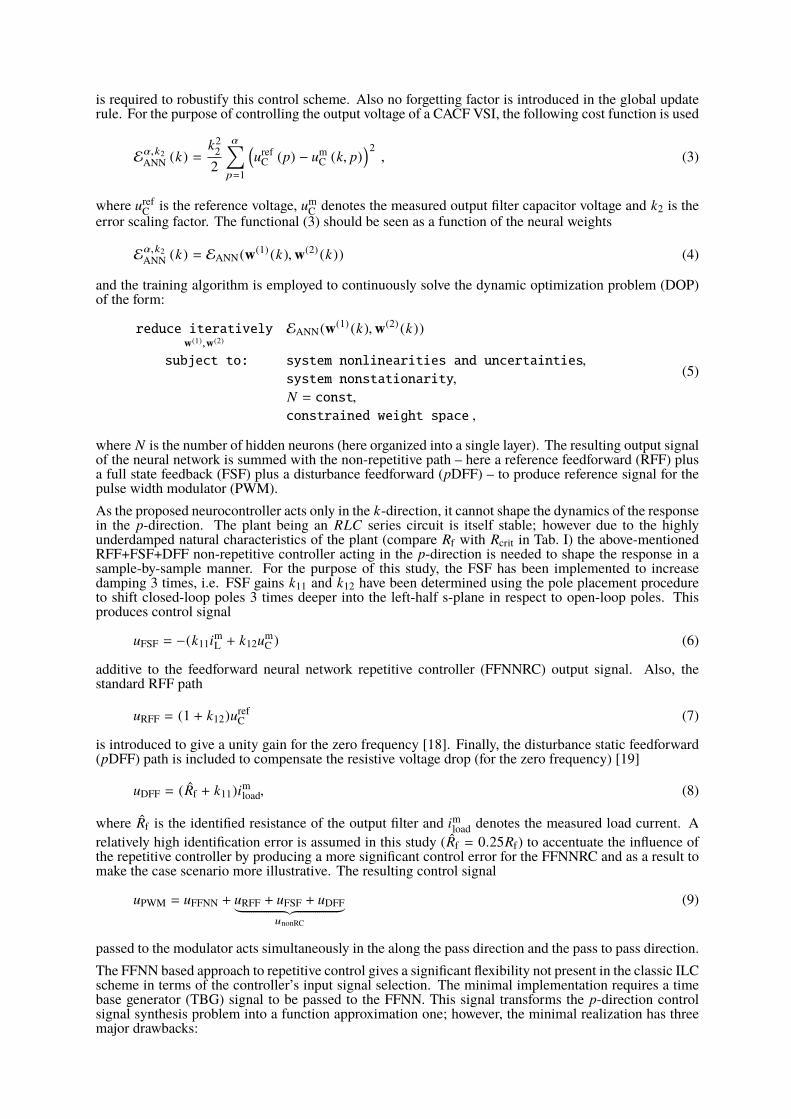
is required to robustify this control scheme. Also no forgetting factor is introduced in the global updaterule. For the purpose of controlling the output voltage of a CACF VSI, the following cost function is used

Eα,k2ANN (k) =

k222

α∑p=1

(urefC (p) − umC (k, p)

)2, (3)

where urefC is the reference voltage, umC denotes the measured output filter capacitor voltage and k2 is theerror scaling factor. The functional (3) should be seen as a function of the neural weights

Eα,k2ANN (k) = EANN(w(1) (k),w(2) (k)) (4)

and the training algorithm is employed to continuously solve the dynamic optimization problem (DOP)of the form:

reduce iterativelyw(1),w(2)

EANN(w(1) (k),w(2) (k))

subject to: system nonlinearities and uncertainties,

system nonstationarity,

N = const,constrained weight space ,

(5)

where N is the number of hidden neurons (here organized into a single layer). The resulting output signalof the neural network is summed with the non-repetitive path – here a reference feedforward (RFF) plusa full state feedback (FSF) plus a disturbance feedforward (pDFF) – to produce reference signal for thepulse width modulator (PWM).As the proposed neurocontroller acts only in the k-direction, it cannot shape the dynamics of the responsein the p-direction. The plant being an RLC series circuit is itself stable; however due to the highlyunderdamped natural characteristics of the plant (compare Rf with Rcrit in Tab. I) the above-mentionedRFF+FSF+DFF non-repetitive controller acting in the p-direction is needed to shape the response in asample-by-sample manner. For the purpose of this study, the FSF has been implemented to increasedamping 3 times, i.e. FSF gains k11 and k12 have been determined using the pole placement procedureto shift closed-loop poles 3 times deeper into the left-half s-plane in respect to open-loop poles. Thisproduces control signal

uFSF = −(k11imL + k12umC ) (6)

additive to the feedforward neural network repetitive controller (FFNNRC) output signal. Also, thestandard RFF path

uRFF = (1 + k12)urefC (7)

is introduced to give a unity gain for the zero frequency [18]. Finally, the disturbance static feedforward(pDFF) path is included to compensate the resistive voltage drop (for the zero frequency) [19]

uDFF = (Rf + k11)imload, (8)

where Rf is the identified resistance of the output filter and imload denotes the measured load current. Arelatively high identification error is assumed in this study (Rf = 0.25Rf) to accentuate the influence ofthe repetitive controller by producing a more significant control error for the FFNNRC and as a result tomake the case scenario more illustrative. The resulting control signal

uPWM = uFFNN + uRFF + uFSF + uDFF︸︷︷︸unonRC

(9)

passed to the modulator acts simultaneously in the along the pass direction and the pass to pass direction.The FFNN based approach to repetitive control gives a significant flexibility not present in the classic ILCscheme in terms of the controller’s input signal selection. The minimal implementation requires a timebase generator (TBG) signal to be passed to the FFNN. This signal transforms the p-direction controlsignal synthesis problem into a function approximation one; however, the minimal realization has threemajor drawbacks:

(a) N = 17 hidden neurons

iteration number k (50 iterations = 1 second)

0 100 200 300 400 500 600

RM

SE

[%

]

0

2

4

6

8

10

350 360

1

2

3

4

only p-direction DFF (pDFF) [blue]

p- and k-direction DDFF [green]

(b) N = 7 hidden neurons


0 100 200 300 400 500 600

RM

SE

[%

]

0

2

4

6

8

10

350 360

1

2

3

4

only p-direction DFF (pDFF) [blue]

p- and k-direction DDFF [green]

Fig. 2: Comparison of the root mean square error (RMSE) decay rates for the Levenberg–Marquardt BP (trainlm)in the case of the classic disturbance feedforward and the novel disturbance dual feedforward.

(a) Bayesian regularization (trainbr)


0 100 200 300 400 500 600

[%]

0

2

4

6

8

10

noise RMS [magenta]

RMSE (error RMS) [blue]

(b) Scaled Conjugate Gradient (trainscg)


0 100 200 300 400 500 600

[%]

0

2

4

6

8

10

noise RMS [magenta]


Fig. 3: Undesired transient states (emphasized using red frames) caused by the regularization mechanism intrainbr, and inconsistent behaviour of trainscg despite identical load variations at time instances 50 s and 450 s– the algorithm failed to track the optimum after the first change in load type.

a) the number of neurons has to be relatively high (ca. 20) to enable effective approximation of controlsignal needed to reject nonlinear load currents that usually do not resemble in shape the TBG signal;and this is an online trained neural network, thus maintaining a low computational burden of thealgorithm, which grows with the number of neurons, is of paramount importance here;

b) the convergence rate is weakened due to the lack of any plant related information at the neural networkinputs;

c) the number of neurons is a trade-off between a precise control signal shaping for significantly nonlinearloads and an absence of excessive overlearning for linear loads and no-load conditions; the minimalrealisation makes working out this trade-off very challenging and the quality of the output voltage hasto be compromised.

A dynamic response in the k-direction improves and the number of neurons can be significantly reducedafter additionally introducing the load current signal at the inputs of the neurocontroller. This is illustratedin Figs. 2a and 2b. The name disturbance dual feedforward (DDFF) is used throughout the paper tohighlight that the load current signal is exploited in both directions.

Choosing the right iterative DOP-capable learning algorithmThe main goal of the research reported in this paper is to identify learning algorithms for a real-timeimplementation. Initially, the Levenberg–Marquardt backpropagation (BP) method was employed andidentified as being able to ensure fast error convergence and high voltage quality at a steady state. However,there exist less computationally demanding learning algorithms such as the resilient backpropagation orBroyden–Fletcher–Goldfarb–Shanno quasi-Newton algorithm. Taking into account that the performanceof any optimization tool is always problem specific, the quality of the output waveform during transientsand at steady states ought to be investigated in the specific system before selecting candidates for practical

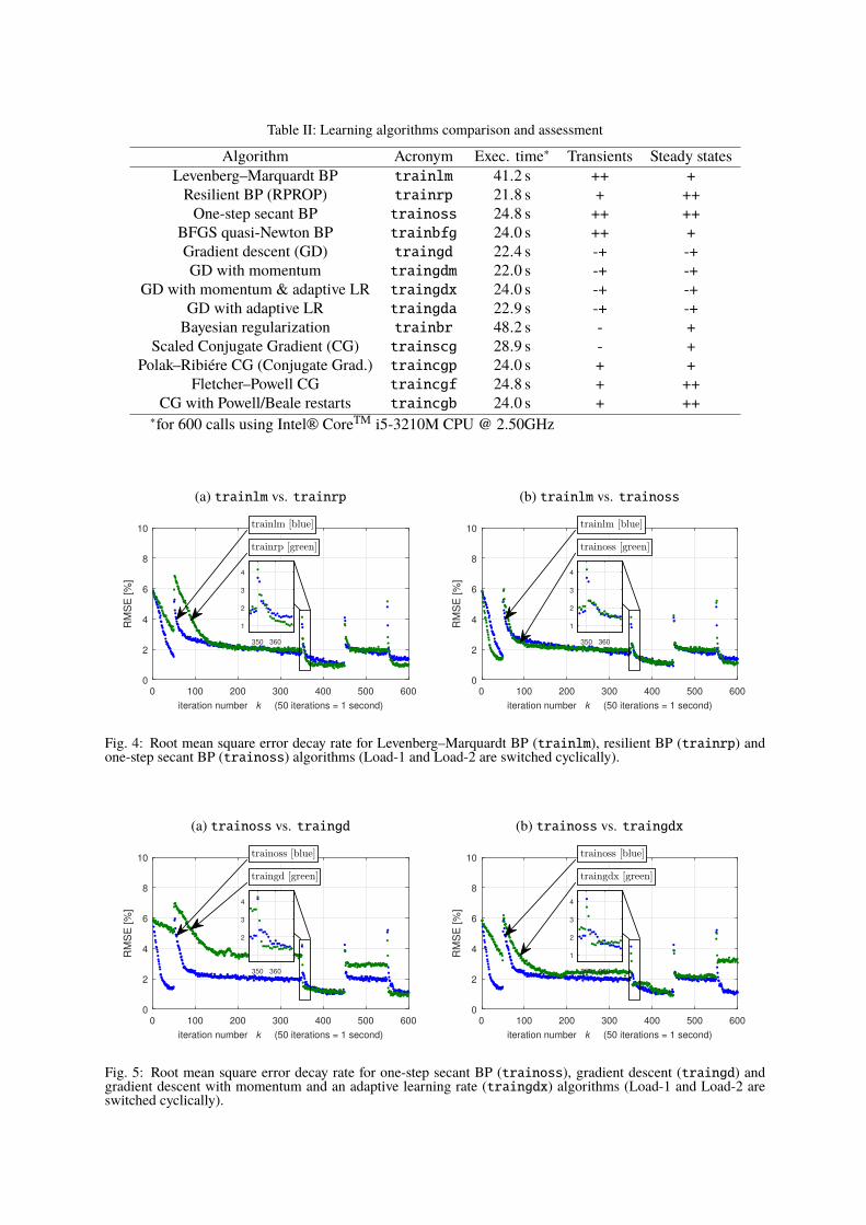
Table II: Learning algorithms comparison and assessment

Algorithm Acronym Exec. time∗ Transients Steady statesLevenberg–Marquardt BP trainlm 41.2 s ++ +Resilient BP (RPROP) trainrp 21.8 s + ++One-step secant BP trainoss 24.8 s ++ ++

BFGS quasi-Newton BP trainbfg 24.0 s ++ +Gradient descent (GD) traingd 22.4 s -+ -+GD with momentum traingdm 22.0 s -+ -+

GD with momentum & adaptive LR traingdx 24.0 s -+ -+GD with adaptive LR traingda 22.9 s -+ -+Bayesian regularization trainbr 48.2 s - +

Scaled Conjugate Gradient (CG) trainscg 28.9 s - +Polak–Ribiére CG (Conjugate Grad.) traincgp 24.0 s + +

Fletcher–Powell CG traincgf 24.8 s + ++CG with Powell/Beale restarts traincgb 24.0 s + ++∗for 600 calls using Intel® CoreTM i5-3210M CPU @ 2.50GHz

(a) trainlm vs. trainrp


0 100 200 300 400 500 600

RM

SE

[%

]

0

2

4

6

8

10

350 360

1

2

3

4

trainlm [blue]

trainrp [green]

(b) trainlm vs. trainoss


0 100 200 300 400 500 600

RM

SE

[%

]

0

2

4

6

8

10

350 360

1

2

3

4

trainlm [blue]

trainoss [green]

Fig. 4: Root mean square error decay rate for Levenberg–Marquardt BP (trainlm), resilient BP (trainrp) andone-step secant BP (trainoss) algorithms (Load-1 and Load-2 are switched cyclically).

(a) trainoss vs. traingd


0 100 200 300 400 500 600

RM

SE

[%

]

0

2

4

6

8

10

350 360

1

2

3

4

trainoss [blue]

traingd [green]

(b) trainoss vs. traingdx


0 100 200 300 400 500 600

RM

SE

[%

]

0

2

4

6

8

10

350 360

1

2

3

4

trainoss [blue]

traingdx [green]

Fig. 5: Root mean square error decay rate for one-step secant BP (trainoss), gradient descent (traingd) andgradient descent with momentum and an adaptive learning rate (traingdx) algorithms (Load-1 and Load-2 areswitched cyclically).

implementation. It should be stressed that these learning algorithms are to be used in a noisy environmentand the optimization task is of a dynamic type. The latter is due to variable load conditions. There is a richvariety of learning algorithms designed for FFNNs training. A majority of them was originally developedas static optimization problem solvers. Nevertheless, most of them can be used in dynamic optimizationproblems without the need of any alterations. Over a dozen off-the-shelf training algorithms available inthe Neural Network Toolbox from MathWorks [20] are tested and compared here. The comparison is byno means a definite one – it refers to only one plant and involves visual assessment of the performanceof the control system. Consequently, only an exemplary decision process is demonstrated and severalrecommendations are made.Selected parameters of the model are collated in Tab. I. It should be noted that all measurements arecorrupted by noise. This makes the search task challenging due to the jagged optimization landscape.Moreover, the task at hand is of a dynamic type, i.e. each training vector (each pass) is presented tothe controller only once (net.trainParam.epochs=1) and then is forgotten completely. The trainingalgorithm directly shapes the dynamics of the controller in the k-direction. Even at a steady state ofthe system the optimisation landscape is still dynamic because of the measurement noise. There areseveral requirements for the weight adaptation mechanism, i.e. the learning algorithm, to be met in orderto facilitate correct operation of the controller under variable load conditions and in the presence of ameasurement noise:

a) the search algorithm should be relatively noise-immune – the effective operation under at least 3%unfiltered measurement noise has to be possible and higher noise levels (up to 10%) should not renderthe search impossible;

b) the algorithm should not stick to an outdated optimum after an abrupt load change, i.e. should be ableto track sudden movements of the optimum;

c) a transition to the new optimal control signal should be smooth to ensure acceptable output voltagequality (uC) during transients;

d) the algorithm should generate consistent results, i.e. a given change in load conditions should alwaysyield similar behaviour of the system.

The test scenario assumes abrupt switchings between two load types: Load-1 and Load-2 (see Tab. Ifor details). The sequence is as follows: Load-1 in the time interval 0–50 s, Load-2 in 50–350 s,Load-1 in the interval 350–450 s, Load-2 in 450–550 s, and at the end again Load-1. If voltage qualitydeteriorates significantly, i.e. beyond noise level, from pass to pass within intervals, this is causedsolely by the learning algorithm itself. Algorithms that offer a near-monotonic decay of the RMSE arepreferable. The consistency of the controller responses is verified using multiple (>3) re-evaluationsin the above-mentioned test scenario. All noise generators have random seeds (rng(’shuffle’)) andalso initial weights are not reproduced from test to test due to the random element of Nguyen-Widrowinitialization [21].Practical implementation of any online trained neurocontroller requires weights to be constricted within acertain range; thus, a mechanism that can effectively prevent weights from overflowing is indispensable.The training with Bayesian regularisation (trainbr) introduces soft limits on weights; however, thecontroller equipped with this algorithm tends to produce undesirable transients illustrated in Fig. 3a. Inthe case of all other algorithms discussed here, hard limits have been imposed on weights. Also thecontroller incorporating the scaled conjugate gradient method (trainscg) failed to produce reproducibleresults in a noisy environment, which is illustrated in Fig. 3b. The rest of the tested algorithms performconsistently throughout experiments and selected observed features are summarized in Tab. II.Often the RPROP is suggested as the first-hand choice for on-line trained non-repetitive neurocon-trollers [22] if the cost function applied is just the squared current control error sample, i.e. weights areupdated after each presentation of a single control error sample (incremental training). The RPROP isreported as providing learning spread equally over the network and, thanks to adaptation affected onlyby the sign of the partial derivative, also less prone to fail due to environment noisiness. It also has thelowest computational complexity. However, other algorithms such as the one-step secant BP (see Fig. 4a)or the BFGS quasi-Newton BP have similar execution time and manifest fast convergence when appliedto the discussed control task. The gradient descent methods struggle to operate effectively in noisymeasurement environment (see Tab. I for the specific noise level) as demonstrated in Fig. 5. All methodstested here are configured as batch ones, i.e. errors are accumulated and all of the weights’ updatesare made at once at the end of a pass. Further study will also include sequential learning algorithms.However, already at this point it can be concluded that as far as the repetitive neurocontroller with theglobal update law is considered there is no definitive winner. The commonly recommended RPROPhas the lowest computational complexity but can be surpassed in terms of convergence rate, e.g, by theone-step memory-less secant method or other full gradient based (in contrast to only gradient sign based)methods as shown in Fig. 4. This may suggest that the related dynamic optimization landscape is onlymoderately challenging and standard learning methods are sufficient to solve the relevant DOP (Fig. 6).

(a) Output capacitor voltage and PWM converteraverage voltage (for trainoss)

0 50 100 150 200

-400V

-325V

0

325V

400V

uC [V]

uVSI

avg [V]

(b) Output capacitor voltage and PWM converteraverage voltage (for trainrp)

0 50 100 150 200

-400V

-325V

0

325V

400V

uC [V]

uVSI

avg [V]

(c) Control error (for trainoss)

0 50 100 150 200

-5%

0

5%

euC

[%]

(d) Control error (for trainrp)

0 50 100 150 200

-5%

0

5%

euC

[%]

(e) Control signal components and load current (fortrainoss)

sample number p

0 50 100 150 200

-400V

-325V

-50V

0

50V

325V

400V

-100A

0

100A

uFFNN

[V]

unonRC

[V]

iload

[A]

(f) Control signal components and load current (fortrainrp)

sample number p

0 50 100 150 200

-400V

-325V

-50V

0

50V

325V

400V

-100A

0

100A

uFFNN

[V]

unonRC

[V]

iload

[A]

(g) Evolution of the output voltage waveform afterconnecting the diode rectifier (for trainoss)

04

iteration number k

k-direction

pass to pass direction

812

1620 (0.4 s)

sample number p

p-direction

along the pass direction

250

200

150

100

50

0

-400

-200

0

200

400

uC

[V

]

(h) Evolution of the output voltage waveform afterconnecting the diode rectifier (for trainrp)

04

iteration number k

k-direction

pass to pass direction

812

1620 (0.4 s)

sample number p

p-direction

along the pass direction

250

200

150

100

50

0

-400

-200

0

200

400

uC

[V

]

Fig. 6: Steady-state waveforms (a)-(f) under diode rectifier load for two algorithms comparable in terms of theirperformance and the evolution of output voltage (g)-(h) after switching from resistive load to diode rectifier load.

(a) 7% measurement noise


0 100 200 300 400 500 600

[%]

0

2

4

6

8

10

noise RMS [magenta]


(b) 10% measurement noise


0 100 200 300 400 500 600

[%]

0

2

4

6

8

10

noise RMS [magenta]


(c) 7% measurement noise

0 50 100 150 200

-5%

0

5%

euC

[%]

(d) 10% measurement noise

0 50 100 150 200

-5%

0

5%

euC

[%]

Fig. 7: Evolution of root mean squared error during transients and steady state performance of the converter underheavy noise conditions – the steady state error along the pass recorded at the time instance of 300 s (the dioderectifier load).

Noise robustness of the repetitive neurocontrollerThe proposed k-direction neurocontroller needs a stable sufficiently damped plant to be plugged into it.The p-direction controller designed using the pole placement method determines the level of damping inthe closed-loop system. The stability of the overall scheme then comes from the convergent optimizationalgorithm. The cost function as well as FSF are here the crucial elements shaping the noise robustnessof the system. However, a more serious noise may require the p-direction controller to be retuned andthis in turn affects the k-direction controller that should also be readjusted, i.e. the learning rate shouldbe modified to work out a new compromise between the responsiveness of the controller and the steadystate performance. The k-direction controller has a strong averaging capability due to the character ofthe cost function (3), which is desirable in the case of white noise. On the other hand, the p-directioncontroller is quite sensitive to noise if its poles are moved far to the left, i.e. high FSF controller gains areintroduced to get strong damping. The highly damped plant makes the optimization task less challengingand hence results in faster convergence – but only if subject to no measurement noise. It is hard topropose a definitive analysis to determine operational noise limits. Nevertheless it has been tested thatthe dynamic neural optimization is still effective under severe noise of 10% (Figs. 7b and 7d), whichis way above noise levels encountered in practical converters. No measurement signal conditioning isintroduced in any of the discussed case scenarios. Clearly, in a steady state the RMSE can drop far belowthe RMS of noise (see e.g. Fig. 7a or Fig. 7b); this happens due to the low-pass characteristics of theplant itself as well as thanks to the averaging nature of the employed functional. Further study will alsoinclude a methodical comparison of levels of immunity against extreme cases of noise for all mentionedalgorithms.

ConclusionA novel robust repetitive neurocontroller with a truly global iterative learning law has been proposed. Theadvantages of a recently developed disturbance dual feedforward concept have been briefly summarised.The performance of the controller has been studied within the context of a pure sine wave inverterand recommendations regarding training algorithms have been made. It has been demonstrated thatthe resilient backpropagation algorithm – a frequent winner in the case of non-repetitive online-trainedneurocontrollers – is not a definitive winner in the case of the repetitive neurocontroller. Other learningalgorithms can operate with similar effectiveness in terms of execution time and offer potentially fasterconvergence rates in this particular application. Important aspects for future study will include theidentification of operational limits in unusually noisy environments and an experimental verification ofthe concept.

References[1] Cichy, B., Galkowski, K., Rogers, E., and Kummert, A.: Control law design for discrete linear

repetitive processes with non-local updating structures, Multidimensional Systems and SignalProcessing, vol. 24, no. 4, 2013, pp. 707–726.

[2] Cichy, B., Galkowski, K., and Rogers, E.: 2D systems based robust iterative learning control usingnoncausal finite-time interval data, Systems & Control Letters, vol. 64, no. 0, 2014, pp. 36–42.

[3] Longman, R. W.: Iterative/repetitive learning control: learning from theory, simulations, andexperiments, Encyclopedia of the Sciences of Learning, Springer US, 2012, pp. 1652–1657.

[4] Elci, H., Longman, R., Phan, M., Juang, J.-N., and Ugoletti, R.: Simple learning control madepractical by zero-phase filtering: applications to robotics, IEEE Transactions on Circuits andSystems I: Fundamental Theory and Applications, vol. 49, no. 6, 2002, pp. 753–767.

[5] Shi, Y.: Robustification in repetitive and iterative learning control, PhD thesis, Columbia Univer-sity, USA, 2013.

[6] Verwoerd,M. H. A.: Iterative learning control – a critical review, PhD thesis, University of Twente,The Netherlands, 2005.

[7] Ufnalski, B. and Grzesiak, L. M.: A performance study on synchronous and asynchronous updaterules for a plug-in direct particle swarm repetitive controller, Archives of Electrical Engineering,vol. 63, no. 4, 2014, pp. 635–646.

[8] Chen, Y. Q., Moore, K., and Bahl, V.: Learning feedforward control using a dilated B-splinenetwork: frequency domain analysis and design, IEEE Transactions on Neural Networks, vol. 15,no. 2, 2004, pp. 355–366.

[9] Deng, H., Oruganti, R., and Srinivasan, D.: Neural controller for UPS inverters based on B-splinenetwork, IEEE Transactions on Industrial Electronics, vol. 55, no. 2, 2008, pp. 899–909.

[10] Ufnalski, B. and Grzesiak, L. M.: Artificial neural network based voltage controller for the sin-gle phase true sine wave inverter – a repetitive control approach, Electrical Review (PrzegladElektrotechniczny), vol. 89, no. 4, 2013, pp. 14–18.

[11] Ufnalski, B. and Grzesiak, L. M.: Particle swarm optimization of an online trained repetitiveneurocontroller for the sine-wave inverter, 39th IECON Annual Conference of the IEEE IndustrialElectronics Society, 2013, pp. 6003–6009.

[12] Kaminski, M., Orlowska-Kowalska, T., and Szabat, K.: Neural speed controller based on two statevariables applied for a drive with elastic connection, 16th International Power Electronics andMotion Control Conference and Exposition (PEMC), 2014, pp. 610–615.

[13] Orlowska-Kowalska, T. and Kaminski, M.: Adaptive Neurocontrollers for Drive Systems: BasicConcepts, Theory and Applications, Advanced and Intelligent Control in Power Electronics andDrives, ed. by Orlowska-Kowalska, T., Blaabjerg, F., and Rodriguez, J., vol. 531, Studies inComputational Intelligence, Springer International Publishing, 2014, pp. 269–302.

[14] Ufnalski, B., Grzesiak, L. M., and Kaszewski, A.: Advanced Control and Optimization Techniquesin AC Drives and DC/AC Sine Wave Voltage Inverters: Selected Problems, Advanced and Intelli-gent Control in Power Electronics and Drives, ed. by Orlowska-Kowalska, T., Blaabjerg, F., andRodriguez, J., vol. 531, Studies in Computational Intelligence, Springer International Publishing,2014, pp. 303–333.

[15] Pajchrowski, T. and Zawirski, K.: Application of artificial neural network for adaptive speed controlof PMSM drive with variable parameters, COMPEL: The International Journal for Computationand Mathematics in Electrical and Electronic Engineering, vol. 32, no. 4, 2013, pp. 1287–1299.

[16] Ufnalski, B. and Grzesiak, L. M.: Particle swarm optimization of artificial-neural-network-basedon-line trained speed controller for battery electric vehicle, Bulletin of the Polish Academy ofSciences: Technical Sciences, vol. 60, no. 3, 2012, pp. 661–667.

[17] Ufnalski, B.: Repetitive Neurocontroller with Disturbance Feedforward, 2014, url: www.mathworks.com/matlabcentral/fileexchange/47867-repetitive-neurocontroller-with-disturbance-feedforward.

[18] Franklin, G., Powell, D., andWorkman, M.:Digital control of dynamic systems, 3rd, Prentice Hall,1997.

[19] Kaszewski, A., Ufnalski, B., and Grzesiak, L. M.: An LQ controller with disturbance feedfor-ward for the 3-phase 4-leg true sine wave inverter, IEEE International Conference on IndustrialTechnology (ICIT), 2013, pp. 1924–1930.

[20] MathWorks: Neural Network Toolbox (MATLAB/Simulink), 2015, url: www.mathworks.com/help/nnet.

[21] MathWorks: Nguyen-Widrow layer initialization function, 2015, url: www.mathworks.com/help/nnet/ref/initnw.html.

[22] Pajchrowski, T., Zawirski, K., and Nowopolski, K.: A neural speed controller trained on-line bymeans of modified RPROP algorithm, IEEE Transactions on Industrial Informatics, vol. 11, no. 2,2015, pp. 560–568.

Documents

Repetitive neurocontroller with disturbance dual