PHYSICAL REVIEW E 88, 013313 (2013)

Replication-based inference algorithms for hard computational problems

Roberto C. Alamino, Juan P. Neirotti, and David SaadNon-linearity and Complexity Research Group, Aston University, Birmingham B4 7ET, United Kingdom

(Received 13 May 2013; published 31 July 2013)

Inference algorithms based on evolving interactions between replicated solutions are introduced and analyzedon a prototypical NP-hard problem: the capacity of the binary Ising perceptron. The efficiency of the algorithm isexamined numerically against that of the parallel tempering algorithm, showing improved performance in termsof the results obtained, computing requirements and simplicity of implementation.

DOI: 10.1103/PhysRevE.88.013313 PACS number(s): 05.10.−a, 84.35.+i

I. INTRODUCTION

One of the main contributions of statistical physics toapplication domains such as information theory and theoreticalcomputer science has been the introduction of establishedmethods that facilitate the analysis of typical properties ofvery large systems in the presence of disorder. For instance,in information theory applications, these large systems corre-spond to (mostly binary) transmissions where the disorder ismanifested through transmission noise or the manner by whichthe message is generated or encoded. Established approachesin the statistical physics community such as the replica andcavity methods [1] have proved to be useful tools in describingtypical properties of error-correcting codes [2–4], the analysisof optimization problems such as the traveling salesman [5],K satisfiability [6], and graph coloring [7,8], to name but afew.

Another important contribution, which complements theones mentioned above, was in the development of algorith-mic tools to find microscopic solutions in specific probleminstances. One of the most celebrated inference methods, themessage-passing (MP) or belief propagation algorithm, hadbeen developed independently in the information theory [9],machine learning [10], and statistical physics [5] communitiesuntil the links between them have been identified [11,12]and established [13]. Subsequently, a number of successfulinference methods have been devised using insights gainedfrom statistical physics [1,14].

In MP algorithms, the system to be solved is mapped onto abipartite factor graph, where on the one hand factor nodescorrespond to observed (given) information or interactionbetween variables; while on the other hand are variablenodes, to be estimated on the basis of approximate marginalpseudoposteriors. The latter are obtained by a set of consistentmarginal conditional probabilities (messages) passed betweenvariable and factor nodes [1]. Unfortunately, there are manycaveats to the MP procedure, especially in the presence ofclosed loops in the factor graph, which may give rise toinconsistent messages and nonconvergence. It can be shownthat MP converges to the correct solution when the factorgraph is a tree, but there is no such guarantee for more generalgraphs, although MP does result in a good solution in manyother cases too.

There are two main general difficulties in using MP algo-rithms to problems represented by densely connected graphs.The first is that the computational cost grows exponentiallywith the degree, making the computation impractical, while

the second arises from the existence of many short loops thatresult in recurrent messages and lack of convergence. Theseproblems have been solved in specific cases, especially inthe case of real observations and continuous noise models byaggregating messages [15]. One of the shortcomings identifiedin Ref. [15] was nonconvergence when prior knowledge on thenoise process is inaccurate or unknown, which typically resultsin multiple solutions and conflicting messages.

While MP would be successfully applied if a weightedaverage over all possible states could be carried out, it isclear that such an average is infeasible. Inspired by thestate-space representation obtained using the replica method[1,5,16] whereby state vectors are organized in an ultrametricstructure, two of us suggested an MP algorithm based onaveraging messages over a structured solutions space [17].The approach is based on using an infinite number of copies(or real replica, not to be confused with those employed inthe replica method) of the variables exposed to the sameobservations (factor nodes). The replicated variable systemsfacilitate a broader exploration of solution space as longas these replica are judiciously distributed according to thesolution-space structure implied by the statistical mechanicsanalysis. The variable vectors inferred by these algorithmsare then combined by taking either weighted or white av-erage to obtain the marginal pseudoposterior of the variousvariables.

The approach has been successful in addressing the codedivision multiple access (CDMA) problem as well as thelinear Ising perceptron capacity problem [18], even in caseswhere prior information is absent. It is worthwhile notingthat a seed of this replication philosophy can be found inseveral previous algorithms such as (a) query by committee[19], where the potential solutions (system replica) are usedfor choosing the best most informative next example andlater combines the solutions using a majority voting; (b) ananalytical approach [20] aimed at obtaining solutions forthe Sherrington-Kirkpatrick model via averages over theThouless-Anderson-Palmer equations; (c) a study of the p-spinmodel metastable states by considering averages over a smallnumber of real replica [21]; (d) the parallel tempering (PT)algorithm, also known as replica exchange Markov chainMonte Carlo (MCMC) sampling, which relies on many replicasearching the space at different temperatures [22,23]; the latter,due to its good performance and relation to the approachwe advocate, will be explained in more detail later on andwill be used for comparison with the method developed here.

013313-11539-3755/2013/88(1)/013313(10) ©2013 American Physical Society

ROBERTO C. ALAMINO, JUAN P. NEIROTTI, AND DAVID SAAD PHYSICAL REVIEW E 88, 013313 (2013)

It is interesting to note that approaches based on averagingmultiple interacting solutions have also been successfully triedin neighboring disciplines, for example, for decoding in thecontext of error-correcting codes [24].

While this approach has been successful in addressinginference problems in the case of real observations andcontinuous noise models, it is less clear as to how it couldbe extended to accommodate more general cases. In thiswork, we will present an alternative method for carryingout averages over the replicated solutions, which can beapplied to more general cases. Generally, like most MP-basedalgorithms, the approach is based on solutions being calculatediteratively using a pair of coupled self-consistent equations.We will study the properties of this alternative algorithm,its advantages and limitations, on an exemplar problem ofthe binary Ising perceptron (BIP) [25,26] that has been usedas a benchmark also in other works on advanced inferencemethods [27].

One obvious obstacle in most MP algorithms is that theiterative dynamics can be trapped in suboptimal minima;in addition, the algorithm itself can either create spurioussuboptimal minima in the already complex solution spaceor change the height of the energy barriers between theexisting ones. We will show that our replica-based MPalgorithm fails under naive averaging of the replica for theBIP capacity problem, explain analytically why it happens,and show that in the limit of a large number of replica,averages flow to the clipped Hebb algorithm [26]. Wewill then propose an alternative approach and show howreplication can indeed improve performance if carried outappropriately.

In Sec. II, we will explain the exemplar problem to beused in this study; we will then review the nonreplicated MPsolution to the BIP capacity problem under the approximationfor densely connected systems in Sec. III and provide ananalytical solution to the naively replicated MP algorithm,showing here its equivalence with the clipped Hebb rule. Sec-tion IV will point to the main reason for the failure of the naivereplica-averaging approach and argue that an online version ofthe MP algorithm, which is derived and presented, can solve it.By replicating the new online MP (OnMP) algorithm and usingthe extra degrees of freedom that it provides, we show how itoutperforms the nonreplicated MP algorithm, termed offlineMP (OffMP) algorithm. Section V compares the replicatedOnMP (rOnMP) with a benchmark parallel algorithm, namely,the PT algorithm. Finally, conclusions and future directions arediscussed in Sec. VI.

II. EXEMPLAR PROBLEM: THE BINARYISING PERCEPTRON

To extend the replica-based inference method [18], wewould like to use an exemplar problem that is particularlydifficult, not only in the worst-case scenario but also typicallywhere both observations and noise model are not real valued.In addition, we would like to examine a case where exactresults have been obtained by the replica theory; this provideshelpful insight in devising the corresponding algorithm bysuggesting a possible structure for the solution space as wellas an analytical tool to assess the efficacy of the algorithm.

One prototypical NP-complete problem [28] that wasshown to be computationally hard even in the typical case,which was solved exactly using the replica method, is thecapacity of the binary Ising perceptron [25]. This is due to thecomplex structure of its solution space studied in Ref. [29],showing a nontrivial topology even in the replica symmetric(RS) phase.

The BIP [26] represents a process whereby K-dimensionalbinary input vectors sμ ∈ {±1}K are received, where the inputvector index μ = 1, . . . ,N , represents each of the N examplevectors. The corresponding outputs for each one of them isdetermined by the binary classification

yμ = sgn

(1√K

K∑k=1

sμkbk

), (1)

where b = (b1, . . . ,bK ) ∈ {±1}K is called the unknown binaryvariables (also referred to as the perceptron’s variable vector);the prefactor

√K is for scaling purposes, so that the argument

of the sign function remains order O(1) as K → ∞.The capacity problem for a BIP is a storage problem,

although it can alternatively be seen as a compression task[30]. In the simplest version of the problem, a data setD = {(sμ,yμ)}N

μ=1 consisting of N pairs of inputs and outputs(also called examples) is randomly generated and a perceptronwith an appropriate variable vector b should be found, suchthat when presented with an input pattern sμ, it reproduces thecorresponding output yμ. That is the equivalent of compressingthe information contained in the set of classifications {yμ},comprising N bits, into a vector b with only K bits. One isusually interested in the typical case, which is calculated byaveraging over all possible data sets D drawn at random froma certain probability distribution.

Typical performance is algorithm dependent and is mea-sured by counting the fraction of correctly stored patternsas a function of the number of examples in the data set.One convenient measure is the average value of the indicatorfunction

χ (b) = 1 −N∏

μ=1

�

(yμ

1√K

K∑k=1

sμkbk

), (2)

with �(· · · ) being the Heaviside step function and b theinferred variable vector. This measure gives 0 if all examplesare correctly stored and 1 otherwise, i.e., it is indicating thatall patterns were perfectly memorized. The maximum valueof α = N/K for which this cost function is 0 (averagedover all possible data sets) is the achieved capacity of thealgorithm and a measure of its overall performance. Thisindicator function was chosen because the BIP capacityproblem focuses on perfect inference of the perceptron’svariable vector b, without allowing for any distortion, ornoise, in the patterns classification. Additionally, it is the mostcommonly used measure in recent publications in this field(e.g., in Ref. [27]).

We use the cost function (2) as a measure used forthe performance of the studied algorithms; however, thealgorithms themselves have been derived by statistical physicsmethods and rely on minimization of an extensive energy given

013313-2

REPLICATION-BASED INFERENCE ALGORITHMS FOR . . . PHYSICAL REVIEW E 88, 013313 (2013)

by the number of misclassified patterns

E(b) =N∑

μ=1

�

(−yμ

1√K

K∑k=1

sμkbk

). (3)

Alternative energy functions were suggested in the liter-ature, for instance [31], and were used in various contexts,especially in the machine learning literature. While thedifferent energy functions tend to share a joint ground state,they may exhibit different behaviors under noisy conditions(imperfect learning, at finite temperatures) as they correspondto different noise models. Although the study of algorithmicperformance at higher temperatures is interesting, it is notwithin the scope of this work, which focuses on examiningthe performance of the suggested algorithm against resultsobtained for the benchmark problem of perfect storage at thenoiseless, zero temperature limit.

It should be noted that the distribution of patterns to bememorized affects the performance of the algorithm. Withinthe class of solvable Ising perceptron capacity problems,patterns sampled from an unbiased distribution constitute themost difficult task. Biased patterns are less informative andare therefore easier to store [32]. We will therefore study onlypatterns generated from unbiased distributions, representingthe most difficult problem, but the method could clearly beextended to accommodate biased patterns.

Although the achieved capacity varies between algorithms,there is an absolute upper bound, the critical capacity αc, abovewhich no algorithm can memorize the whole set of examplesin the typical case (although it might be possible for specificinstances); this reflects the information content limit of theperceptron itself.

The critical capacity was calculated by Krauth and Mezardusing the one-replica symmetry breaking (1RSB) ansatz [25]with the result of αc ≈ 0.83. Taking into consideration that theproblem is computationally hard, the challenge then becomesto find an algorithm which infers appropriate b values in typicalspecific instances of D as close as possible to αc, where thecorresponding computational complexity scales polynomiallywith the system size.

III. NAIVE MESSAGE PASSING

The inference problem we aim to address is finding themost appropriate value of the variable vector b capable ofreproducing the classifications given the examples data set D.First, one needs to determine a quality measure that quantifiesthe appropriateness of a solution. The most commonly usederror measure in similar estimation problems is the expectederror per variable, or bit-error-rate in the information theoryliterature, the minimization of which leads to a solution basedon the marginal posterior maximizer (MPM) estimator givenby

bk = argmaxbk∈{±1}∑bl �=k

P(b|D) = sgn〈bk〉P(b|D), (4)

which means that one estimates b bitwise, such that eachcomponent bk corresponds to the variable value that maximizesthe marginal distribution per variable given the data set D. The

MP equations allow one to carry out an approximate Bayesianinference procedure to find this estimator.

It is important to remember that there might not exist avariable vector capable of reproducing the whole data set. Inthis case, the data set is unrealizable by the BIP, althoughone can still identify the most probable candidate. In the BIPcapacity problem, unrealizable data sets exist since they aregenerated randomly, not by a teacher perceptron as is the casein some generalization problems. Each variable in the set D isdrawn from an independent distribution and therefore one canwrite the posterior distribution of the variable vector as

P(b|D) = P(b|{yμ},{sμ}) ∝ P({yμ}|b,{sμ})P(b), (5)

where P({yμ}|b,{sμ}) factorizes as the examples are sampledidentically and independently

P({yμ}|b,{sμ}) =N∏

μ=1

P(yμ|b,sμ). (6)

From the Bayesian point of view, P(b) is interpreted as the(factorized) prior distribution of possible variable vectors.As there is no noise involved in the capacity problem, thelikelihood factor is simply given by

P(yμ|b,sμ) = 1

2+ yμ

2sgn ξμ, (7)

defining

ξμ = 1√K

K∑k=1

sμkbk. (8)

As for each instance the data set is fixed, we will omit inthe following expressions the explicit reference to the inputvectors sμ in the posterior distribution for brevity.

The resulting MP equations are self-consistent coupledequations of marginal conditional probabilities which areiterated until convergence (or up to a cutoff number ofiterations). These equations are obtained by applying Bayestheorem to each one of the so-called Q messages and R

messages

Qt+1μk (bk) = P t+1(bk|{yν �=μ})

∝ P(bk)∏ν �=μ

P t+1(yν |bk,{yσ �=ν}), (9)

Rt+1μk (bk) = P t+1(yμ|bk,{yν �=μ})

=∑{bl �=k}

P(yμ|b)∏l �=k

P t (bl|{yν �=μ}), (10)

where P(bk) is the prior distribution over the kth entry of thevariable vector and t stands for the current iteration step.

As bk ∈ {±1}, one can write

Qt (bk) = 1 + mtμkbk

2and Rt (bk) ∝ 1 + mt−1

μk bk

2. (11)

The variables mμk may be interpreted as magnetization relatedto the cavity field in analogy to spin lattices in magneticfields. The interpretation of the mμk variables is less intuitive.Substituting the R messages into the Q messages and summingover the two possible values of bk , we finally reproduce the

013313-3

ROBERTO C. ALAMINO, JUAN P. NEIROTTI, AND DAVID SAAD PHYSICAL REVIEW E 88, 013313 (2013)

MP equations in their well-known form

mtμk =

∑bk

bkP t+1(yμ|bk,{yν �=μ})∑bkP t+1(yμ|bk,{yν �=μ}) , (12)

mtμk = tanh

⎡⎣∑

ν �=μ

atanh mtνk

⎤⎦ ≈ tanh

⎛⎝∑

ν �=μ

mtνk

⎞⎠. (13)

The approximation in the last equation is possible since mμk ∼O(1/

√K) as we will see later.

Once convergence is attained, the value for the variablevector can be estimated by

bk = sgn mk, (14)

mk = tanh

(∑ν

mtνk

), (15)

or

bk = sgn

(∑ν

mtνk

). (16)

As mentioned in Sec. II, the factor graph representingthe BIP is densely connected, but an expansion for large K

suggested by Kabashima [15] helps to simplify the equationsaway from criticality. However, for the BIP this expansionrequires extra care due to the discontinuity of the sign function.To address this problem, we developed a different approach tocarry out this expansion which can be generalized to accommo-date other types of perceptrons with minimal modifications; itcan be applied to either continuous or discontinuous activationfunctions, with or without noise. Equation (13) for mμk is notmodified, but mμk is expanded in powers of 1/

√K , giving

rise to a different expression (detailed derivation is providedin Appendix A):

mμk = 2sμkyμ√K

Nμk

1 + erf(yμuμk/

√2σ 2

μk

) , (17)

where

Nμk = 1√2πσ 2

μk

exp

(− u2

μk

2σ 2μk

), (18)

σ 2μk = 1

K

∑l �=k

(1 − m2

μl

), (19)

uμk = 1√K

∑l �=k

mμlsμl. (20)

However, this version of the algorithm is unable tomemorize large numbers of examples. Simulation results showthat, even for small system sizes (K ∼ 10), it can not memorizemore than a single pattern on average. This is a consequence ofthe fact that the dynamical map defined by the MP equationsbecomes trapped in the many suboptimal minima of the energylandscape.

In principle, one should be able to correct this by replicatingthe system and distributing the n replica randomly in solutionspace, let each one carry out the inference task independently,and compare their final fixed points. An idea along these lines,with a small number of real replica searching the space inparallel, was tested with some success in Ref. [21], where the

replica helped change the landscape to facilitate jumps overbarriers between metastable states. However, the correspond-ing algorithm was not very efficient computationally. Also,the replicated version of MP we tested failed and the observedperformance coincided with that of the nonreplicated version.

To understand the reasons for the failure of the naivelyreplicated algorithm, we solved the replicated version of thealgorithm analytically. We consider the case where a simplewhite average of the n replica is used for inferring the variablevector value

bk = sgn

(1

n

n∑a=1

bak

). (21)

We can then evaluate the MP equations using a saddle pointmethod when n,N,K → ∞. The detailed calculation is givenin Appendix B, giving rise to a surprisingly simple final result

bk = sgn

⎛⎝ N∑

μ=1

yμsμk

⎞⎠. (22)

Simplicity is not the only surprising aspect of this result. Thosefamiliar with past research in machine learning will readilyrecognize this equation as the clipped version of the Hebblearning rule [33]. Unfortunately, this is not good news asthe maximum attainable capacity by this algorithm has beenalready calculated analytically to be NH

K≡ αH =≈ 0.11 [34,

35]. Worse yet, the achieved capacity of the clipped-Hebbrule quickly deteriorates as K increases, converging to zeroasymptotically.

The flow of the replicated algorithm towards the clippedHebb rule points out some other weaknesses of the MPalgorithm. It is not difficult to appreciate that MP results ina clipped rule as the final estimate of the variable vector isobtained by clipping the fixed point of the magnetization; thisimplies that it suffers from all pathologies present in clippedrules such as suboptimal solutions.

Another characteristic that is highlighted by this result isthe fact that, like the Hebb rule, the MP approach is an offline(batch) learning algorithm in the sense that it does not dependon the order of presentation of the examples. This is true bothfor the nonreplicated and replicated algorithms. This suggeststhat one could introduce an extra source of stochasticity bydevising an online version of the MP, which could allow for thealgorithm to overcome the energy barriers that trap it in localminima. Different orders of examples correspond to differentpaths in solution space which, combined, could potentiallyexplore it much more efficiently. The examples order is anextra degree of freedom that can not be exploited in offlinealgorithms. In the following section, we show that by pursuingthis idea, we find a replicated version of MP which does notonly perform better than the offline one (OffMP), but alsooffers many additional advantages.

IV. ONLINE MESSAGE PASSING

The results of the previous section indicate that replicationof the OffMP algorithm does not offer any significant improve-ment in performance in the BIP capacity problem. The onlineversion of the MP algorithm introduced here allows one to

013313-4

REPLICATION-BASED INFERENCE ALGORITHMS FOR . . . PHYSICAL REVIEW E 88, 013313 (2013)

exploit the order of presentation of examples as a mechanismto avoid algorithmic trapping in local minima. This algorithmwill then be used in its replicated version with a polynomialnumber of replica n with respect to the number of examplesN .

In order to develop an online version of the MP algorithm,we rely on a large K expansion. When K → ∞, one canderive the equations for the magnetization (mean values) ofthe inferred variable vector [Eq. (15)] as

mk = tanh

(∑ν

mνk

)

= tanh

⎛⎝∑

ν �=μ

mνk + mμk

⎞⎠

≈ tanh

⎛⎝∑

ν �=μ

mνk

⎞⎠ + mμk

⎡⎣1 − tanh2

⎛⎝∑

ν �=μ

mνk

⎞⎠

⎤⎦

= mμk + [1 − (mμk)2]mμk. (23)

Equation (23) singles out the μth example similarly tothe OffMP derivation. However, in the online interpretationit is considered a new example, being presented sequentiallyafter all previous μ − 1 examples have been learned. Then,mk can be interpreted as the updated magnetization, whilemμk is the magnetization linked to the cavity field inducedby the previous examples, before example μ is included.In the bipartite interpretation of the model, this is akin tothe introduction of new a factor node, exploiting conditionalprobabilities calculated with respect to the previous μ − 1examples. To make this interpretation more explicit, we add atime label to the obtained equation by changing mk to mk(t),mμk to mk(t − 1), and considering the μth example as theexample being presented at time t . The online MP algorithmcan finally be written as

mk(t) = mk(t − 1) + stkyt√K

Fk(t), (24)

with the so-called modulation function given by

Fk(t) = 2[1 − m2

k(t − 1)] Ntk

1 + erf(ytutk/

√2σ 2

tk

) , (25)

where

σ 2tk = 1

K

∑l �=k

[1 − m2

l (t − 1)], (26)

utk = 1√K

∑l �=k

stlml(t − 1). (27)

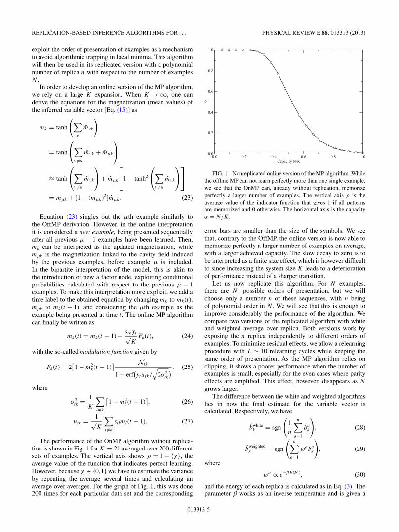
The performance of the OnMP algorithm without replica-tion is shown in Fig. 1 for K = 21 averaged over 200 differentsets of examples. The vertical axis shows ρ = 1 − 〈χ〉, theaverage value of the function that indicates perfect learning.However, because χ ∈ {0,1} we have to estimate the varianceby repeating the average several times and calculating anaverage over averages. For the graph of Fig. 1, this was done200 times for each particular data set and the corresponding

0.0 0.2 0.4 0.6 0.8 1.0Capacity N/K

0.0

0.2

0.4

0.6

0.8

1.0

ρ

FIG. 1. Nonreplicated online version of the MP algorithm. Whilethe offline MP can not learn perfectly more than one single example,we see that the OnMP can, already without replication, memorizeperfectly a larger number of examples. The vertical axis ρ is theaverage value of the indicator function that gives 1 if all patternsare memorized and 0 otherwise. The horizontal axis is the capacityα = N/K .

error bars are smaller than the size of the symbols. We seethat, contrary to the OffMP, the online version is now able tomemorize perfectly a larger number of examples on average,with a larger achieved capacity. The slow decay to zero is tobe interpreted as a finite size effect, which is however difficultto since increasing the system size K leads to a deteriorationof performance instead of a sharper transition.

Let us now replicate this algorithm. For N examples,there are N ! possible orders of presentation, but we willchoose only a number n of these sequences, with n beingof polynomial order in N . We will see that this is enough toimprove considerably the performance of the algorithm. Wecompare two versions of the replicated algorithm with whiteand weighted average over replica. Both versions work byexposing the n replica independently to different orders ofexamples. To minimize residual effects, we allow a relearningprocedure with L ∼ 10 relearning cycles while keeping thesame order of presentation. As the MP algorithm relies onclipping, it shows a poorer performance when the number ofexamples is small, especially for the even cases where parityeffects are amplified. This effect, however, disappears as N

grows larger.The difference between the white and weighted algorithms

lies in how the final estimate for the variable vector iscalculated. Respectively, we have

bwhitek = sgn

(1

n

n∑a=1

bak

), (28)

bweightedk = sgn

(n∑

a=1

wabak

), (29)

where

wa ∝ e−βE(ba ), (30)

and the energy of each replica is calculated as in Eq. (3). Theparameter β works as an inverse temperature and is given a

013313-5

ROBERTO C. ALAMINO, JUAN P. NEIROTTI, AND DAVID SAAD PHYSICAL REVIEW E 88, 013313 (2013)

high value in order to select lower energy states. Clearly, whenβ = 0, the white and weighted averages are the same.

We compared the performance of the two versions ofthe rOnMP against the nonreplicated one. Both performmuch better than the nonreplicated algorithm. The differencebetween weighted and white averages in related problems hadalready been studied in relation to the TAP equations via thereplica approach yielding similar results [20]; this indicatesthat similar problems appear in the corresponding dynamicalmaps. Contrary to our expectations, though, we have not foundany difference in performance between the weighted and whiteaveraged algorithms. This seems to indicate that even selectionof the best performers as done by the weighted average is notenough to prevent the algorithm of being trapped in suboptimalsolutions, which can only be avoided by increasing the numberof replica.

It is interesting to note that a variational approach carriedout by Kinouchi and Caticha [36] was successful in finding theoptimal online learning rule for a perceptron, in the sense thatit will saturate the Bayes’ generalization bound calculated byOpper and Haussler [37]. Although the perceptron generaliza-tion problem is different from the capacity problem, as in theformer, the data set is clearly realizable having been generatedby a corresponding perceptron, which might not be the case forthe latter; up to the critical capacity one can assume that the setof random examples, in the typical case, is indeed realizable.In fact, this is usually one of the underlying assumptions whenattempting to solve the capacity problem. This means that wecan use the same algorithms to carry out both tasks.

The precise form for the parallel variational optimal (VO)algorithm for the BIP was derived in Ref. [38] and is given by

b(t + 1) = b(t) + st yt√N

F (t), (31)

where the modulation function is

F (t) = 2

√Q(t)

R(t)2[1 − R(t)2]

× Nt

1 + erf(R(t)φ(t)/√

2(1 − R(t)2)), (32)

with

R(t) = b0 · b(t)

|b0||b(t)| , Q(t) = b(t)2

N,

(33)

φ(t) = h(t)yt , h(t) = b · st

|b| ;

where b0 is a teacher perceptron, which in the capacity casewould correspond to the correct inferred variable vector, thetrue value of which we do not know. In employing the VOalgorithm, an assumption that the overlaps are self-averaginghas been used. Therefore, a sensible way to obtain a value thatcould be used as a good estimate of b0 is to run the algorithmmany times in parallel and average all values of b(t) at eachiteration. Like in our algorithm, this average can be eitherwhite or weighted.

A notable characteristic of the above set of equations is theirsimilarity with our equations for the OnMP if one substitutes

mk → bk, m2k → R2, Rφ → yu, 1 − R2 → σ 2, (34)

respectively. In fact, the asymptotic behavior of the VOguarantees that even the square-root amplitude appearing infront of the modulation function tends to the same value asin the OnMP, making the two sets isomorphic under thissubstitution. This striking relation between both algorithmsis a strong indication that our algorithm must also becapable of achieving the optimal capacity and saturates Bayes’generalization bound [37].

V. PERFORMANCE

In this section, we compare the performance of the rOnMPwith that of the PT algorithm. The reason for choosing PTis that it is a well established parallel algorithm with goodperformance in searching for solutions in the BIP capacityproblem. Other derivatives of BP-based algorithms havebeen used to solve the BIP capacity problem, for instance,survey propagation [6,27]; the latter also aims to addressthe fragmentation of solution space but employs a differentapproach. The results reported [6,27] show that solutions canbe found very close to the theoretical limits even for largesystems, but additional practical techniques and considerationsshould be used to successfully obtain solutions. As ouraim in this work is to show how replication can improvesignificantly the performance of MP algorithms, we use thePT algorithm as the preferred benchmark method due to itssimpler implementation.

Parallel tempering (PT) or replica exchange Monte Carloalgorithm [22,23] was introduced as a tool for carrying outsimulations of spin glasses. Like the BIP capacity problem,spin glasses have a complicated energy landscape with manypeaks and valleys of varying heights and PT has beensuccessfully applied to that and many other similar problemswhere the extremely rugged energy landscape causes othermethods to underperform [39,40].

In many cases, searching for the low energy states isdone by gradient descent methods. In statistical physics,simulated annealing is a principled and useful alternative togradient descent by allowing for a stochastic search whileslowly decreasing the temperature; it is particularly effectivein the cases where the landscape has one or very fewvalleys. However, to guarantee convergence to an optimalstate, the temperature should be lowered very slowly and mostapplications use a much faster cooling rate. In the case of spinglasses, this causes the algorithm to be easily trapped in localminima.

The idea behind the PT algorithm is to introduce a numberof replica of the system that search the solution space in parallelat different temperatures using a simple Metropolis-Hastingsprocedure. The higher the temperature, the easier it is for thereplica to jump over energy barriers, but convergence becomesincreasingly compromised. However, jumping over barriersallows for the exploration of a large part of solution space, andthe PT algorithm cleverly exploits this by comparing, at chosentime intervals, the energy of the present random walker at twodifferent successive temperatures. If the higher-temperaturerandom walker reaches a state of smaller energy than the one ata lower temperature, they are exchanged, otherwise there is anexponentially small probability for this exchange to take place;

013313-6

REPLICATION-BASED INFERENCE ALGORITHMS FOR . . . PHYSICAL REVIEW E 88, 013313 (2013)

0.5 1.0 1.5α

0.0

0.2

0.4

0.6

0.8

1.0

ρ

Parallel TemperingOnline MP / n=10000

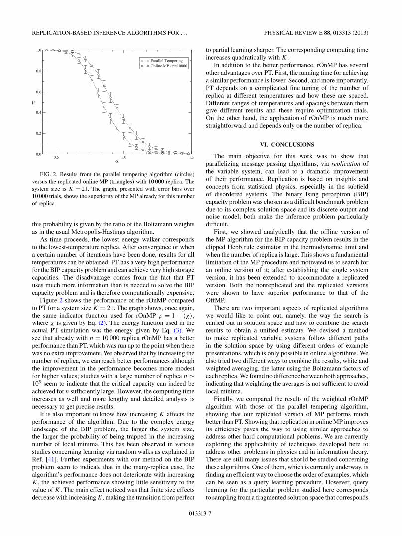
FIG. 2. Results from the parallel tempering algorithm (circles)versus the replicated online MP (triangles) with 10 000 replica. Thesystem size is K = 21. The graph, presented with error bars over10 000 trials, shows the superiority of the MP already for this numberof replica.

this probability is given by the ratio of the Boltzmann weightsas in the usual Metropolis-Hastings algorithm.

As time proceeds, the lowest energy walker correspondsto the lowest-temperature replica. After convergence or whena certain number of iterations have been done, results for alltemperatures can be obtained. PT has a very high performancefor the BIP capacity problem and can achieve very high storagecapacities. The disadvantage comes from the fact that PTuses much more information than is needed to solve the BIPcapacity problem and is therefore computationally expensive.

Figure 2 shows the performance of the rOnMP comparedto PT for a system size K = 21. The graph shows, once again,the same indicator function used for rOnMP ρ = 1 − 〈χ〉,where χ is given by Eq. (2). The energy function used in theactual PT simulation was the energy given by Eq. (3). Wesee that already with n = 10 000 replica rOnMP has a betterperformance than PT, which was run up to the point when therewas no extra improvement. We observed that by increasing thenumber of replica, we can reach better performances althoughthe improvement in the performance becomes more modestfor higher values; studies with a large number of replica n ∼105 seem to indicate that the critical capacity can indeed beachieved for n sufficiently large. However, the computing timeincreases as well and more lengthy and detailed analysis isnecessary to get precise results.

It is also important to know how increasing K affects theperformance of the algorithm. Due to the complex energylandscape of the BIP problem, the larger the system size,the larger the probability of being trapped in the increasingnumber of local minima. This has been observed in variousstudies concerning learning via random walks as explained inRef. [41]. Further experiments with our method on the BIPproblem seem to indicate that in the many-replica case, thealgorithm’s performance does not deteriorate with increasingK , the achieved performance showing little sensitivity to thevalue of K . The main effect noticed was that finite size effectsdecrease with increasing K , making the transition from perfect

to partial learning sharper. The corresponding computing timeincreases quadratically with K .

In addition to the better performance, rOnMP has severalother advantages over PT. First, the running time for achievinga similar performance is lower. Second, and more importantly,PT depends on a complicated fine tuning of the number ofreplica at different temperatures and how these are spaced.Different ranges of temperatures and spacings between themgive different results and these require optimization trials.On the other hand, the application of rOnMP is much morestraightforward and depends only on the number of replica.

VI. CONCLUSIONS

The main objective for this work was to show thatparallelizing message passing algorithms, via replication ofthe variable system, can lead to a dramatic improvementof their performance. Replication is based on insights andconcepts from statistical physics, especially in the subfieldof disordered systems. The binary Ising perceptron (BIP)capacity problem was chosen as a difficult benchmark problemdue to its complex solution space and its discrete output andnoise model; both make the inference problem particularlydifficult.

First, we showed analytically that the offline version ofthe MP algorithm for the BIP capacity problem results in theclipped Hebb rule estimator in the thermodynamic limit andwhen the number of replica is large. This shows a fundamentallimitation of the MP procedure and motivated us to search foran online version of it; after establishing the single systemversion, it has been extended to accommodate a replicatedversion. Both the nonreplicated and the replicated versionswere shown to have superior performance to that of theOffMP.

There are two important aspects of replicated algorithmswe would like to point out, namely, the way the search iscarried out in solution space and how to combine the searchresults to obtain a unified estimate. We devised a methodto make replicated variable systems follow different pathsin the solution space by using different orders of examplepresentations, which is only possible in online algorithms. Wealso tried two different ways to combine the results, white andweighted averaging, the latter using the Boltzmann factors ofeach replica. We found no difference between both approaches,indicating that weighting the averages is not sufficient to avoidlocal minima.

Finally, we compared the results of the weighted rOnMPalgorithm with those of the parallel tempering algorithm,showing that our replicated version of MP performs muchbetter than PT. Showing that replication in online MP improvesits efficiency paves the way to using similar approaches toaddress other hard computational problems. We are currentlyexploring the applicability of techniques developed here toaddress other problems in physics and in information theory.There are still many issues that should be studied concerningthese algorithms. One of them, which is currently underway, isfinding an efficient way to choose the order of examples, whichcan be seen as a query learning procedure. However, querylearning for the particular problem studied here correspondsto sampling from a fragmented solution space that corresponds

013313-7

ROBERTO C. ALAMINO, JUAN P. NEIROTTI, AND DAVID SAAD PHYSICAL REVIEW E 88, 013313 (2013)

to the replica symmetry breaking solution space and demandsthe introduction of a carefully constructed interaction betweenthe replicated solutions, which we currently investigate.

ACKNOWLEDGMENT

Support by the Leverhulme trust (F/00 250/M) is acknowl-edged.

APPENDIX A: MESSAGE PASSING EXPANSION FOR THEBINARY ISING PERCEPTRON

Consider the first MP equation (12), repeated as follows forconvenience:

mtμk =

∑bk

bkP t+1(yμ|bk,{yν �=μ})∑bkP t+1(yμ|bk,{yν �=μ}) . (A1)

We denote the numerator of this expression simply by A,ignoring for brevity the dependence on the indices. Byintroducing a variable ξ to represent the field ξμ using a Diracdelta, we can write

A = yμ

2K

∫dξ dξ

2πeiξ ξ (sgn ξ )

×⎡⎣∏

l �=k

∑b

(1 + mμlb) exp

(−iξ

sμlb√K

)⎤⎦

×∑

b

b exp

(−iξ

sμkb√K

). (A2)

Summing over b ∈ {±1}, one obtains

∑b

(1 + mμkb) exp

(−iξ

sμkb√K

)

= 2

[cos

(ξ√K

)− imμksμk sin

(ξ√K

)]

≈ 2

[1 − imμksμk

ξ√K

− ξ 2

2K

], (A3)

where, in the last line, we expand the trigonometric functionsto their first nontrivial orders in 1/

√K , already taking into

consideration the large K scenario. By doing the sameexpansion to the second summation, one obtains

∑b

b exp

(−iξ

sμkbk√K

)= −2isμk sin

(ξ√K

)

≈ −2isμk

ξ√K

. (A4)

These approximations allow one to rewrite the expressionfor A as

A = −iyμsμk√K

∫dξ dξ

2πeiξ ξ (sgn ξ )ξ

× exp

[∑l

ln

(1 − ξ 2

2K− imμlsμl

ξ√K

)]

≈ −iyμsμk√K

∫dξ

2π(sgn ξ )

∫dξ ξ

× exp

[− ξ 2σ 2

μk

2+ iξ (ξ − uμk)

], (A5)

where

σ 2μk = 1

K

∑l �=k

(1 − m2

μl

), uμk = 1√

K

∑l �=k

mμlsμl. (A6)

The resulting integral is trivial and, by following the analogoussteps for the denominator, we finally reach the result given byexpression (17).

APPENDIX B: ANALYTICAL DERIVATION OF THEREPLICATED NAIVE MP ALGORITHM

Upon replication of the variable system such that the finalestimate of the variable vector is inferred by a white averageof the n replica

bk = sgn

(1

n

n∑a=1

bak

), (B1)

one can take the limit n → ∞ to calculate a closed expressionfor it. The MP equations (12) and (13) remain the same, butthe likelihood term has to include the contribution of thereplica as

P(yμ|b) =∑{ba}

P(yμ|b,{ba})P({ba}|b), (B2)

P(yμ|b) = 1

2n+1

[1 + yμ sgn

(1√K

K∑k=1

sμkbk

)] ∏a

[1 + yμ sgn

(1√K

K∑k=1

sμkbak

)], (B3)

P({ba}|b) ∝∏k

1

2

[1 + bk sgn

(1

n

n∑a=1

bak

)]. (B4)

In the last equation, we ignore the normalization. For the calculation to be carried out rigorously, the normalization should betaken into account in what follows. However, careful calculations show that it does not change the saddle point result. The aboveexpressions can be substituted in the first of the MP equations (12). Let us concentrate on the numerator of Eq. (12), which can

013313-8

REPLICATION-BASED INFERENCE ALGORITHMS FOR . . . PHYSICAL REVIEW E 88, 013313 (2013)

be written as

A ∝∫ [

dξ dξ

2πeiξ ξ

][∏a

dξadξ a

2πeiξa ξ a

](1 + yμ sgn ξ )

∏a

(1 + yμ sgn ξa)∑

b

bk

⎡⎣∏

l �=k

1

2(1 + blmμl)

⎤⎦ exp

⎡⎣− iξ√

K

K∑j=1

sμjbj

⎤⎦

×∑{ba}

∏j

1

2

[1 + bj sgn

(1

n

n∑a=1

baj

)]exp

⎡⎣− i√

K

∑a

ξ a

K∑j=1

sμjbaj

⎤⎦. (B5)

To decouple the replicated systems, we introduce the K variables

λk = 1

n

∑a

bak , (B6)

via Dirac deltas. By defining the notation

D[ξ,ξ ] ≡[dξ dξ

2πeiξ ξ

][∏a

dξadξ a

2πeiξa ξ a

], D[λ,λ] ≡

[∏k

dλkdλk

2π/neinλkλk

], (B7)

and summing over b’s, we obtain

A ∝∫

D[λ,λ]D[ξ,ξ ](1 + yμ sgn ξ )∏a

(1 + yμ sgn ξa)

⎡⎣∏

a,j

cos

(λj + ξ asμj√

K

)⎤⎦[

− i sin

(ξ sμk√

K

)+ sgn λk cos

(ξ sμk√

K

)]

×∏l �=k

(1 + mμl sgn λl)

[cos

(ξ sμl√

K

)− i sgn λl sin

(ξ sμl√

K

)]. (B8)

One can now expand the arguments of the cos and sin functions in powers of 1/√

K to obtain

A ∝∫

D[λ,λ]D[ξ,ξ ](1 + yμ sgn ξ )∏a

(1 + yμ sgn ξa) exp

⎡⎣∑

a,j

ln

(cos λj − ξ asμj√

Ksin λj − (ξ a)2

2Kcos λj

)⎤⎦

×(

−iξ sμk√

K+ sgn λk

)exp

⎡⎣∑

l �=k

ln(1 + mμl sgn λl) +∑l �=k

ln

(1 − ξ 2

2K− iξ√

Ksgn λl

)⎤⎦. (B9)

The integrals over the ξ variables are easy to calculate, leadingto the following expression at leading order in 1/

√K:

A ∝∫ ⎡

⎣∏j

dλjdλj

2π/n

⎤⎦sgn λk en , (B10)

where

= i∑

j

λj λj + 1

n

∑l �=k

ln (1 + mμlsgn λl)

+∑

j

ln cos λj + 1

n

n∑c=0

ln Ic, (B11)

with

Ia = 1 + yμerf

⎛⎝ uμ√

2σ 2μ

⎞⎠, a = 1, . . . ,n (B12)

uμ = − i√K

∑j

sμj tan λj , (B13)

σ 2μ = 1

K

∑j

(1 + tan2 λj

), (B14)

I0 = 1 + yμerf

(u0

μk√2

), (B15)

u0μk = 1√

K

∑l �=k

sμl sgn λl. (B16)

Following the same calculations for the denominator, onecan see that for large n the variables mμk are given by sgn λ∗

k ,where λ∗

k is defined by the saddle point of the integral (B10),

which is a solution of the simultaneous equations

∂

∂λj

= ∂

∂λj

= 0. (B17)

Differentiating we finally find the result

mμk = yμsμk, (B18)

resulting in the estimate (22) of the variable vectors that alsocorresponds to the clipped Hebb rule.

013313-9

ROBERTO C. ALAMINO, JUAN P. NEIROTTI, AND DAVID SAAD PHYSICAL REVIEW E 88, 013313 (2013)

[1] M. Mezard and A. Montanari, Information, Physics, andComputation (Oxford University Press, Oxford, UK, 2009).

[2] D. Saad, Y. Kabashima, T. Murayama, and R. Vicente, inCryptography and Coding, Lecture Notes in Computer Science,edited by B. Honary, Vol. 2260 (Springer, Berlin, 2001),pp. 307–316.

[3] R. C. Alamino and D. Saad, Phys. Rev. E 76, 061124 (2007).[4] R. C. Alamino and D. Saad, J. Phys. A: Math. Theor. 40, 12259

(2007).[5] M. Mezard and G. Parisi, J. Phys. (Paris) 47, 1285 (1986).[6] A. Braunstein, M. Mezard, and R. Zecchina, Random Struct.

Alg. 27, 201 (2005).[7] J. van Mourik and D. Saad, Phys. Rev. E 66, 056120 (2002).[8] R. Mulet, A. Pagnani, M. Weigt, and R. Zecchina, Phys. Rev.

Lett. 89, 268701 (2002).[9] R. G. Gallager, Research Monograph Series, 21 (MIT Press,

Cambridge, MA 1963).[10] J. Pearl, Probabilistic Reasoning in Intelligent Systems: Net-

works of Plausible Inference (Morgan Kaufmann, San Francisco,1988).

[11] Y. Kabashima and D. Saad, Europhys. Lett. 44, 668 (1998).[12] M. Opper and D. Saad, Advanced Mean Field Methods-Theory

and Practice (MIT Press, Cambridge, MA, 2001).[13] J. S. Yedidia, W. T. Freeman, and Y. Weiss, IEEE Trans. Inf.

Theory 51, 2282 (2005).[14] M. Mezard, G. Parisi, and R. Zecchina, Science 297, 812 (2002).[15] Y. Kabashima, J. Phys. A: Math. Gen. 36, 11111 (2003).[16] H. Nishimori, Statistical Physics of Spin Glasses and Informa-

tion Processing (Oxford University Press, Oxford, UK, 2001).[17] J. P. Neirotti and D. Saad, Europhys. Lett. 71, 866 (2005).[18] J. P. Neirotti and D. Saad, Phys. Rev. E 76, 046121 (2007).[19] H. Seung, M. Opper, and H. Sompolinsky, in COLT ’92

Proceedings of the Fifth Annual Workshop on ComputationalLearning Theory (ACM, New York, 1992), pp. 287–294.

[20] C. De Dominicis, M. Gabay, T. Garel, and H. Orland, J. Phys.(Paris) 41, 923 (1980).

[21] J. Kurchan, G. Parisi, and M. A. Virasoro, J. Phys. I (France) 3,1819 (1993).

[22] R. H. Swendsen and J.-S. Wang, Phys. Rev. Lett. 57, 2607(1986).

[23] E. Marinari and G. Parisi, Europhys. Lett. 19, 451 (1992).[24] S. Kudekar, T. J. Richardson, and R. L. Urbanke, IEEE Trans.

Inf. Theory 57, 803 (2011).[25] W. Krauth and M. Mezard, J. Phys. (Paris) 50, 3057 (1989).[26] A. Engel and C. van den Broeck, Statistical Mechanics of

Learning (Cambridge University Press, Cambridge, UK, 2001).[27] A. Braunstein and R. Zecchina, Phys. Rev. Lett. 96, 030201

(2006).[28] L. Pitt and L. G. Valiant, J. Assoc. Comput. Mach. 35, 965

(1988).[29] T. Obuchi and Y. Kabashima, J. Stat. Mech. (2009) P12014.[30] T. Hosaka, Y. Kabashima, and H. Nishimori, Phys. Rev. E 66,

066126 (2002).[31] H. Horner, Z. Phys. B 86, 291 (1992).[32] E. Gardner, J. Phys. A: Math. Gen. 21, 257 (1988).[33] H. Kohler, S. Diederieh, W. Kinzel, and M. Opper, Z. Phys. B:

Condens. Matter 78, 333 (1990).[34] H. Sompolinsky, Phys. Rev. A 34, 2571 (1986).[35] J. L. van Hemmen, Phys. Rev. A 36, 1959 (1987).[36] O. Kinouchi and N. Caticha, Phys. Rev. E 54, R54 (1996).[37] M. Opper and D. Haussler, Phys. Rev. Lett. 66, 2677

(1991).[38] J. P. Neirotti, J. Phys. A: Math. Theor. 43, 015101 (2010).[39] J. P. Neirotti, F. Calvo, D. Freeman, and J. D. Doll, J. Chem.

Phys. 112, 10340 (2000).[40] J. P. Neirotti, F. Calvo, D. Freeman, and J. D. Doll, J. Chem.

Phys. 112, 10350 (2000).[41] H. Huang and H. Zhou, J. Stat. Mech. (2010) P08014.

013313-10