Embed Size (px)
Citation preview

Reply to Jonathan Morduch’s
“Does Microfinance Really Help the Poor?
New Evidence from Flagship Programs in Bangladesh”
Mark M. Pitt
Department of Economics
Brown University
October 14, 1999
I benefitted from the comments of Shahidur R. Khandker, Andrew Foster, Nidhiya Menon, and
Chris Udry.

I. Introduction
This paper addresses the concerns raised by Jonathan Morduch in his paper “Does
Microfinance Really Help the Poor? New Evidence from Flagship Programs in Bangladesh”
about the methods and results of Mark M. Pitt and Shahidur R. Khandker, “The Impact of
Group-Based Credit Programs on Poor Households in Bangladesh: Does the Gender of
Participants Matter?” in the Journal of Political Economy, 1988, Vol. 106, No. 5, hereafter
referred to as PK. Morduch makes five major criticisms of PK:
1)The eligibility cut-off of one-half acre of land owned is often violated, and this violation results
in substantial bias in the PK estimates;
2)The restrictive way in which PK introduce village fixed effects to control for important
components of unobserved heterogeneity fails to distinguish between eligible and ineligible
households and thus is likely to result to bias;
3)”New evidence” in the form of simple difference-in-differences estimates using both de facto
and de jure eligibility rules fail to find positive program effects;
4)The higher positive impacts of female credit as compared to male credit on household
consumption may simply reflect diminishing marginal returns;
5)The linear functional form used by PK is insufficiently flexible. Nonlinearities in the effects of
explanatory variables may cause the PK estimates to be positively biased.
Section 2 of the paper addresses each of these criticisms and finds them lacking because
Morduch has misunderstood and mischaracterized the methods of PK, and has applied incorrect
methods to obtain his new evidence. In order to present the reader with a clearer demonstration
of the methods adopted by PK, as compared to those of Morduch, an appendix provides a set of

2
simulation programs in the form of Stata™ do-files that simulate the processes by which these
credit programs, by gender, are allocated across villages, how eligible household make
participation decisions, and how these participation decisions affect household outcomes (such as
consumption).
II. Response to Morduch’s criticisms
A.“Mistargeting” of program eligibility biases the results
Morduch notes that a significant proportion of program households report owning more
land than the de jure eligibility amount of ½ acre. The eligibility rule of these credit programs is
in terms of cultivable land. Table 1 presents data on the size distribution of cultivable land
owned by program participating households at the time they joined a credit program. In the
aggregate, a bit over 17 percent of program households had more than ½ acre of land at the time
they joined a credit program. The Grameen Bank, with 21.1 percent, has the greatest proportion
of “mistargeted” households. The difference between total land ownership and cultivable land
ownership is primarily homestead land. Many poor households, even those without any
cultivable land, often have a very small plot of land containing an extremely small shelter and
perhaps a small garden. Some also possess uncultivable waste land. Average total land owned is
only 14 hundredths of an acre larger than cultivable land owned.
Although Morduch makes much of land purchases by program households, they are in
fact quite small on average in our sample. Table 2 presents the average total land and cultivable
land owned at the time of the survey. These average landholdings increased by only 6 one-
hundredths of an acre since the time of joining. Morduch reports that only half of the land
acquisitions were purchases, most of the remaining acquisition were inheritance. If the average
size of inherited plots were equal to the average size of purchased plots, purchases of land would
amount to only 3 one-hundredths of an acre, or 121 square meters.
What constitutes “cultivable” land for the purposes of program eligibility is ambiguous.
Many household have uncultivable or nearly uncultivable land, such as char lands that lie within
river dikes. These lands cannot be cultivated during the peak season as they form part of a river

1The importance of eroded char lands in Bangladesh is unfortunately quite evident andgrowing. On a recent trip to Rangpur district, I had the opportunity to visit one of our surveyareas in which recent movements of the Teesta and Jamuna rivers has turned well-off farmersinto destitute farmers in a few years. These farmers still own this newly eroded land and mayplant some of it during the boro season, but it cultivation quality is so poor that it bears littleresemblance to its pre-eroded state. One household in particular has gone from being one of thewealthiest cultivating households in the village to one of destitution in which the household headspends most of his time working as a wage laborer.
2Hossein (1988, p. 25) provides further evidence that land quality matters in thedetermination of eligibility. He notes that after 1983 “a person from a household that owns lessthan 0.5 acres of cultivated land, or assets with a value equivalent to less than 1.0 acre ofmedium-quality land, is eligible to receive a loan.” (my underlining)
3
bed during that season. In the dry season, these lands are poorly suited to agriculture as a
consequence of erosion, and property rights to them are poorly established since any plot
markers and water containment bunds are washed away in the seasonal floods.1 These credit
programs are likely aware of the differential cultivability of plots of land, and might be expected
to make adjustments for land quality in judging the eligibility of a household.2
There is a simple way to test whether this might be so with our data. The data set
contains information on the current market value of land. If the credit programs take the quality
of land into consideration in determining eligibility, that is, use some quality adjusted notion of
efficiency units of land, then the unit price of land in participating households with more than ½
acre should be less than the unit price of land of other households with similar quantities of land.
Table 3 presents results from estimating the determinants of unit land prices with our data. The
results of five regressions are presented, two estimated by ordinary least squares and three with
thana-level fixed effects. All specifications demonstrate quite conclusively that “mistargeted”
households, that is, participating households owning more than ½ acre of total land at the time of
the survey, have dramatically lower land values even after conditioning on total land area and its
square, participant status and thana fixed effects. The mean unit value of land for those owning
land is Taka 1484 per decimal. Consequently, conditional on the other regressors, mistargeted
households have unit land values of about one-half that of households which are not mistargeted.
To put this into perspective, the average unit value of all landholding for households owning

4
more than 50 decimals of land is Taka 791 per decimal while the estimated decline in unit land
value associated with being a “mistargeted “ household is Taka 721 per decimal (column 5). All
of which suggests that these credit programs are doing a better job of targeting than a first look at
the data would have us believe.
This apparent use of efficiency units of land in determining eligibility on the part of these
credit programs does not completely resolve the econometric issue of using eligibility criteria as
the basis for parameter identification. The problem is that land quality is unobserved and thus we
cannot be certain that a household with, say, 0.75 acres, is not a program participant because it is
ineligible, or is not because it is eligible (perhaps because it’s land is char land or barely
cultivable), but chooses not to participate. The problem of appropriately classifying households
does not disappear. Morduch’s approach is to apply the de jure eligibility rule in estimating
program effects. He gives no justification for this, and indeed there is none. If there is a “soft”
(de facto) eligibility rule that takes land quality or other considerations (including lying or
corruption) into account, there is no reason why one should get consistent estimates of program
effects by imposes the wrong (de jure) eligibility rule on the data. Indeed, it is easy to show that
taking program households with more than ½ acre of land and treating them as ineligible is
precisely the wrong direction to take. The much better procedure is to take nonprogram
households with somewhat more than ½ acre of land and treat them as if they have choice, not to
take program households and treat them as if they are not program participants. Dropping from
the sample those households owning more that ½ acre of land that are program participators
imparts classical sample selection bias to any estimates of program effects.
By raising the eligibility cutoff to land ownership greater than ½ acre, say one acre, all
households, whether program participant or not, are treated as having the choice to participate.
In this way, those who really do have choice but choose not to participate are now treated
appropriately. On the other hand, some of these households that are not program participants
with land below 1 acre are actually ineligible. However, this classification error does not alter
the consistency of the estimates of program effects. Treating a behavior as endogenous when it is
in fact exogenous still yields consistent estimates. It merely reduces the efficiency of those
estimates. This is akin to having uncertainty about the endogeneity of independent variables in a

3When there are limited dependent variables things become a bit murkier. Treatinghouseholds without program choice as choosing to not participate in the program alters theempirical distribution of the credit participation errors and consequently, since the distribution ofthe errors matter in the limited dependent variable model, the parameter estimates may alsochange.
5
regression or the appropriateness of random versus fixed effects. Treating a possibly exogenous
regressor as endogenous (with instrumental variables methods) results in consistent estimates
whether that regressor is exogenous or endogenous. Similarly, treating the time-persistent
component of the residual as a fixed effect results in consistent parameter estimates even if this
component is in fact orthogonal to the regressors and could have been treated as a random effect.
Bias results only when endogenous behavior is treated as exogenous, not when exogenous
behavior is treated as endogenous. The simulation program sim12.do in the appendix to this
paper demonstrates this result numerically in the case of two-stage least squares.3
Understanding whether de facto land classification (“mistargeting”) matters to the results
of PK is ultimately purely an empirical issue upon which Morduch’s approach sheds no light.
What remains to be seen is whether raising the land ownership cutoff to values above ½ acre will
reduce or increase our earlier estimates of program effects based on the de jure cut off for
nonpartipating households and the actual (de facto) cut off for participating households. This is
actually a simple task. One just needs to re-estimate the model at higher land cutoff’s, treating
more and more households as having endogenous choice rather than no choice, and see how
parameter estimates respond. In the results reported below, we reclassify households as having
the choice to join a microcredit program at land ownership values of 0.66, 1.20, 1.60 and 2.00
acres. Based upon the discussion above, we can hypothesize how estimated program effects
would change at higher eligibility cut offs. Since Pitt and Khandker (1998) treated participating
households with more than ½ acre of land as households with choice (endogenous), the source of
any bias arises from incorrectly treating nonparticipating households with more than ½ acre of
land who actually had choice as not having choice. If our earlier finding that higher consumption
households are less likely to be credit program participants, conditional on the regressors, is true,
then putting these “high” consumption households incorrectly into the control group rather than
the treatment (choice) group would tend to underestimate program effects. Consequently, PK

4In Pitt and Khandker (1998), households with more than 5.0 acres of land were droppedfrom the analysis to aid comparability. In the case of a 2.0 acre eligibility rule (Table 4, column5), we have added these households back into the analysis for two reasons. First, five acres ofland is certainly more comparable to 2 acres than it is to ½ acre. Second, the sample size of“control” households gets small as more households are deemed eligible for “treatment”.
6
underestimate program effects. Choosing successively higher eligibility cutoffs should actually
increase the estimated program effects. In fact the problem of signing the change is a bit more
complicated than this, but this intuition reflects the first-order effects.
Table 4 provides estimates of the determinants of the logarithm of per capita household
consumption with five different eligibility rules. The estimates of column (1), exactly
reproduced from Table 2 in Pitt and Khandker (1998), are based on the de jure rule for
nonparticipators and the (unknown) de facto rule for participators. The other four columns have
progressively higher land ownership eligibility rules.4 As Table 1 notes, there are 157
participating households with cultivable land in excess of 0.50 acres prior to joining the program.
With the imposed eligibility rules there are 127, 62, 46 and 28 program households with land
owned in excess of the 0.66, 1.20, 1.60 and 2.0 acre rules, respectively. Consequently, as we
progressively raise the de facto program eligibility rule, over 82 percent of the previously
“mistargeted” participating household are moved to within the eligibility rule. In the case of the
1.6 acre eligibility rule, about 5 percent of sample observations in program villages are
considered “non-choice” observations, as compared to 10 percent with the 0.5 acre rule.
The estimated program effects in Table 4 reveal that under the ½ acre rule, Pitt and
Khandker (1998) did indeed slightly underestimate the consumption returns to female program
credit, and slightly overestimate the consumption returns to male program credit. The qualitative
conclusions of Pitt and Khandker (1998), that there are significant and large returns to female
borrowing and smaller and insignificant returns to male borrowing, is only strengthened by the
results of Table 4. If all households with land ownership of less than or equal to 2.0 acres, a level
of land ownership four times the de jure rule, are treated as having the choice to join the
program, the effect of female credit program participation on consumption rises about 20 percent,
and the asymptotic t-statistics rise by about 80 percent. This pattern, along with the pattern of
algebraically smaller (more negative) correlation coefficients (D) for women, is consistent with

5If an eligibility rule is fuzzy in that actual eligibility rule applied is a fixed value plus arandom variable, the use of the PK procedure results in consistent estimates even if the value ofthe random variable is unknown, that is, even if the incorrect de jure eligibility rule is used in theeconometrics. This result does not require that the random variable have zero mean. Applicationof this consistency result to these data does not seem reasonable in this case, nor is it necessary. This special case is illustrated in the simulation programs sim9.do and sim10.do presented in theappendix.
7
the view that low expenditure households, conditional on a large set of regressors that include
land area unadjusted for land quality, aremore likely to have women become credit program
participants. That is, this result is consistent with having the relative cultivation quality of land
taken into consideration in determining eligibility.5
B. Village fixed effects are incorrectly specified and unduly parsimonious
Morduch criticizes PK’s approach of controlling for village fixed effects, suggesting that
if programs locate on the basis of qualities specific only to target groups, that village fixed effects
as implemented by PK may not be an improvement, but may exacerbate bias by setting up the
wrong benchmark (p. 9). To make his point, he characterizes PK’s framework with regression
equation (1), reproduced here:
(M1)
where eiv indicates eligibility status of household i in village v irrespective of whether a program
is in fact available in village v, bv indicates program availability in village v, the vector of X’s
control for household characteristics, the dv are village-level dummy variables, and ,iv is an
idiosyncratic error term. The coefficient "1 is the difference-in-difference, the impact over and
above the village mean -- the effect of eligibility status on the outcome Yiv. There is no
disagreeing with Morduch’s statement that bias could arise in this framework:
“The problem arises since the programs explicitly limit their attention to just

6The simulation programs beginning with sim6.do illustrate how fixed effects are actuallyspecified in PK.
8
functionally landless households. Thus, the critical unobservables will be those
specific to target groups within villages, not just unobservables that affect all
villagers equally. “(p. 9)
The problem is that Morduch mischaracterizes the approach of PK. In fact, PK do exactly what
Morduch claims should be done in the above quoted paragraph. That this, they explicitly allow
for program availability to be responsive to the unobservables of only the target groups within
villages. In PK, the “first-stage” credit reduced form demand equations are estimated over the
subsample of (de facto) eligible households in villages with a program since they are the only
ones who can join and borrow. Credit is deterministically zero for all villages without a program
and for all ineligible households in program villages. There is no credit program behavior to be
estimated at all as there is no element of choice. In PK’s paper, these first-stage equations
(equation1 for the case that does not consider gender, and equations 6 and 7 for the case that
does) all have village fixed effects which are clearly separate and distinct from another set of
fixed effects affecting the outcome Y (equations 2 and 8). Yet Morduch’s characterization of PK
given by his equation (1) and the ensuing discussion, incorrectly suggests that there is but one
village fixed effect per village in the PK estimation, and none specific to target households. In
actuality, the first-stage equations of PK have two fixed effects (one per gender) specific only to
the target households (of each gender) of each village with a credit program, and a village fixed
effect for the outcome equation of villages. 6
That this is the case in PK is quite clearly stated in their paper. Reproduced below are
equations (6) and (7 ) from PK:
(6)
(7)

9
where Cijf and Cijm is the program credit obtained by females and males, respectively, in
household i of village j, :cjf and :c
jm are unmeasured determinants of Cij that are fixed within a
village, the X are observed household characteristics and the $cm are parameters to be estimated.
The “second-stage” outcome equation in PK (equation 8) is:
(8)
where $y and * are unknown parameters, :yj is an unmeasured determinant of yij that is fixed
within a village, and distinct from the fixed effects :cjf and :c
jm. The log-likelihood presented as
equation (5) in PK for the case without gender distinction, and in the Appendix to PK for the
case with gender distinction, also clearly distinguishes separate fixed effects to control for the
placement of credit programs from fixed effects that control for the effect of village
unobservables on the behavior Y. The log-likelihood presented as equation (5) in PK (pages
968-969) and relevant parts of its discussion is reproduced verbatim below:
“ Distinguishing between households not having choice because they reside in a non-
program village and households residing in a program village that do not have choice
because of the application of an exogenous rule (landowning status), and suppressing the
household and village subscripts i and j, the likelihood can be written as:
(5)
where M2 is the bivariate standard normal distribution, M is the univariate standard
normal distribution, :cp are the village-specific effects influencing participation in the
credit program in program villages, :yp are village-specific effects influencing the binary
outcome Iy in program villages, :yn are the corresponding village-specific effects in
nonprogram villages, and dc = 2*Ic - 1 and dy= 2*Iy - 1. The errors ,cij and ,y
i j are
normalized to have unit variance and correlation coefficient D. Village-specific effects

10
(:cn) influencing the demand for program credit are not identifiable for villages that do
not have programs.
The first part of the likelihood is the joint probability of program
participation and the binary outcome Iy conditional on participation for those
households that are both eligible to join the program (choice) and reside in a village
with the program (program village).” (Italics in original, boldface added for
emphasis)
Thus, the fixed effects that determine the availability of a credit program is estimated over “ those
households that are both eligible to join the program (choice) and reside in a village with the program
(program village).” I am not sure that this could be said any clearer. That these fixed effects are
specific to the eligible (target) households is also implied from the number of observations used
in estimating the first-stage credit demand equation list in Table 2 (1105 for women and 895 for
men, significantly less than the number used in the second-stage equations), and from footnote 4
which states that over 200 village fixed effects are estimated, but there are just 87 villages in the
complete sample of which 72 have credit programs. How could Morduch’s characterization of
one fixed effect per village be consistent with these numbers? Indeed, as the paper makes clear,
there are three fixed effects in villages with male and female credit programs, two fixed effects
with only a female or male credit program, and one fixed effect if there is no credit program.
Furthermore, all of the credit demand fixed effects are explicitly limited to functionally landless
(target) households. The large number of fixed effects seems inconsistent with a claim that PK
were unduly parsimonious with them.
One might have the impression that I have cited more evidence than required to convince
the average reader of my claim. In a number of communications with Morduch, I repeatedly
stressed the point that there is no program choice for the ineligible, and that consequently the
demand for credit and its village dummy variables pertain only to the eligible. All of which
make his mischaracterization of PK all the more surprising. It appears that Morduch has some
appreciation for these communications since with equations (4) and (5) of his pages 23 and 24 he
once again offers a characterization of the instrumental variable method of PK. The top line of
his equation (4) (reproduced below) has deterministic credit for the ineligible

11
(3)
That he understands this zero to be deterministic rather than stochastic, and thus unavailable to
identify any credit demand parameters, is clear from the first line of text after he presents
equations (4) and (5). There he states, “Apart from the first line of equation (4), this is a standard
instrumental variables problem.” ( 24-35) This line ends with a footnote beginning “I thank
Mark Pitt for stressing the importance of this distinction.”
C. Morduch’s “new evidence”
Morduch presents new estimates of credit program effects in his Tables 6 through 11.
These tables present difference-in-differences estimates using both de jure and de facto eligibility
rules. We have already noted that the use of the de jure eligibility rule is unjustified and will
likely result in a biased estimate of program effects. However, failure to adequately deal with the
mistargeting issue is not the only mistake to bedevil Morduch’s new evidence. He fails to set out
a clear framework justifiying his difference-in-the-differences estimate, so it might be hard to see
what the issues are. It seems that his estimate is simply the application of the identification
example of PK, reproduced from Pitt and Khandker (1998, p. 968) below:
“To illustrate the identification strategy, consider a sample drawn from two
villages -- village 1 does not have the program and village 2 does; and, two types
of households, landed (Xij=1) and landless (Xij=0). Innocuously, we assume that
landed status is the only observed household-specific determinant of some
behavior yij in addition to any treatment effect from the program. The conditional
demand equation is:
The exogeneity of land ownership is the assumption that E(Xij,,yij) = 0, that is, that

12
land ownership is uncorrelated with the unobserved household-specific effect.
The expected value of yij for each household type in each village is:
E(yij | j=1, Xij=0) = :y1 (4a)
E(yij | j=1, Xij=1) = $y + :y1 (4b)
E(yij | j=2, Xij=1) = $y + :y2 (4c)
E(yij | j=2, Xij=0) = p* + :y2 (4d)
where p is the proportion of landless households in village 2 who choose to
participate in the program. It is clear that all the parameters, including the effect
of the credit program *, is identified from this design.”
The estimator of the program effect * in equation (4d) is the differences-in-the-
differences estimator widely applied in the general program evaluation literature. To see this,
note that an estimate of * is obtained from the following difference-in-the-differences, labeled as
equation (a);
p* = [E(yij | j=2, Xij=0) - E(yij | j=2, Xij=1)] - [E(yij | j=1, Xij=0) - E(yij | j=1, Xij=1)] (a)
The estimates that Morduch present in his tables (6) through (11) are, as far as I can tell, based
on (a). The problem is that while (a) represents that difference-in-the-differences estimator of
the program effect * in the illustrative example of PK above, it is likely to provide a biased
estimate of program effects when applied to our data. This bias simply reflects the difference
between an experiment, in which both observable attributes and unobservable attributes have the
same expections in both the treatment and control groups, and a quasi-experiment in which they
do not. Our data clearly conform to a quasi-experiement. Morduch treats them as if they
conform to an experiment. To see the problem this error causes, take the outcome equation (3), in
which Xij is a vector of observed household characteristics, and difference once:

7It is odd indeed that after arguing that these credit programs are likely to limit theirattention to the functionally landless in making program placement decision, and thus it is theirunobservables that matters, Morduch ignores his own advice in calculating his new estimates.
13
(b)
here j=2 indicates a credit program village , eij=1 indicates a target household, * is “the impact
over and above the village mean and the fact of being ‘eligible’ ” (Morduch p. 9), and the village
fixed effect in this solved out equation varies between eligible (target) households and ineligible
(nontarget) households, as in the actual application of PK. The negative of the remainder in (b)
are the “differences” estimates of * presented by Morduch in the last row of each of the tables 6
through 11. However, for this to represent the true differences requires that (X02 - X01)$y + (:02 -
:01) = 0. Morduch himself strenuously argues that there is no reason to believe that (:02 - :01) =
0.7 In addition, is it reasonable to expect that (X02 - X01)$y = 0? This equality would hold if the
means of the observed characteristics of poor target households are the same as the mean
observed characteristics of the richer nontarget households, an equality that would be implied
from experimental assignment to treatment and control groups. But households are not
experimentally assigned to the Grameen Bank. Eligible household’s choose to join on the basis
of observed and unobserved characteristics. Similarly, the Grameen Bank chooses to serve a
village on the basis of observed and unobserved village characteristics that differ on average
between eligible (target) households and ineligible (nontarget) households. These observed
characteristics, which in PK include level of schooling, sex of household head, presence of males
in the household, existence of landed non-coresident relatives, and land owned, are not the same,
on average, between rich and poor. The only hope is that differencing the differences of the
program and nonprogram village would alleviate this problem. That difference-in-the
differences is:
8In addition, the X’s and the :’s are correlated. See below.
9The pattern of credit effects on consumption reported in Pitt and Khandker (1998) Table4 (p. 985) are consistent with a finding that Morduch’s difference-in-the-difference’s estimate aredownward biased. The instrumental variable estimates that control for household self-selectioninto credit programs but do not include for village fixed effects (labeled WESML-LIML)
14
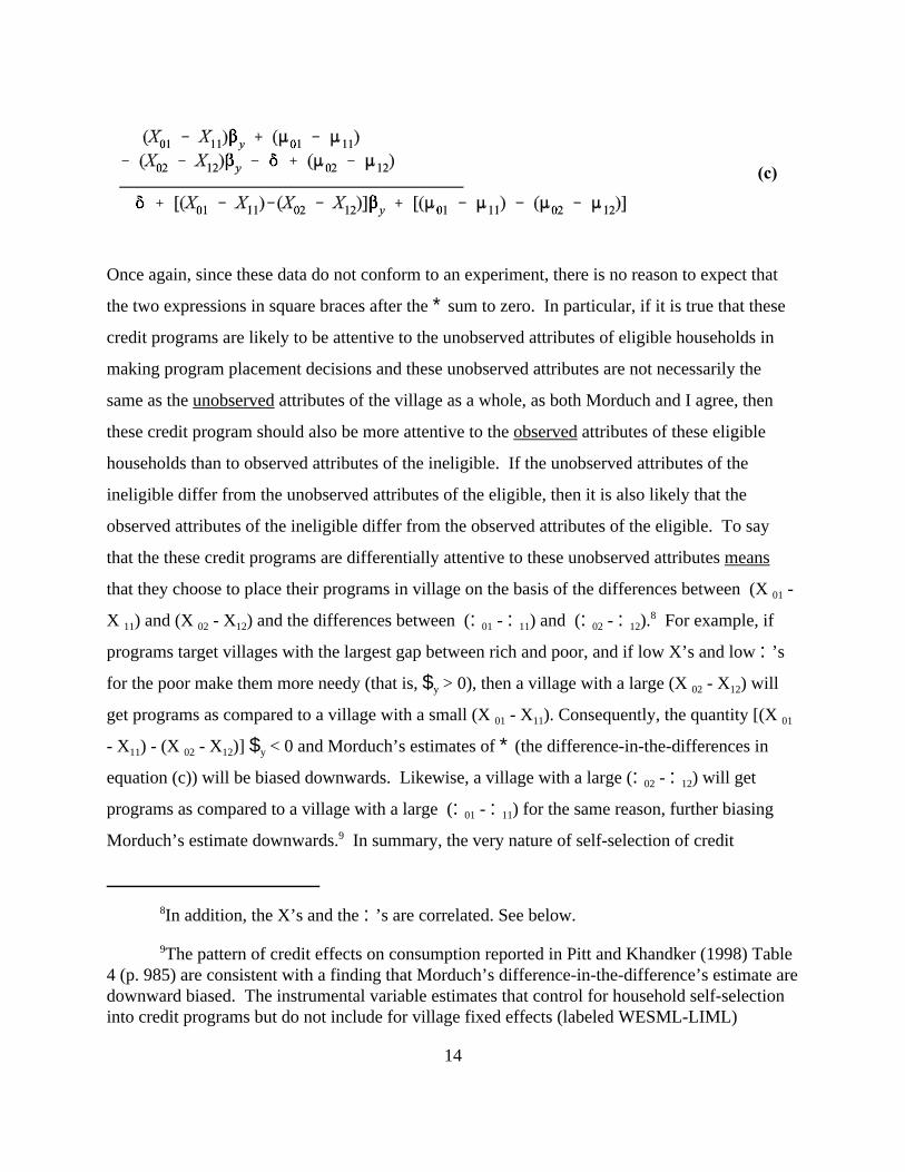
(c)
Once again, since these data do not conform to an experiment, there is no reason to expect that
the two expressions in square braces after the * sum to zero. In particular, if it is true that these
credit programs are likely to be attentive to the unobserved attributes of eligible households in
making program placement decisions and these unobserved attributes are not necessarily the
same as the unobserved attributes of the village as a whole, as both Morduch and I agree, then
these credit program should also be more attentive to the observed attributes of these eligible
households than to observed attributes of the ineligible. If the unobserved attributes of the
ineligible differ from the unobserved attributes of the eligible, then it is also likely that the
observed attributes of the ineligible differ from the observed attributes of the eligible. To say
that the these credit programs are differentially attentive to these unobserved attributes means
that they choose to place their programs in village on the basis of the differences between (X 01 -
X 11) and (X 02 - X12) and the differences between (:01 - :11) and (:02 - :12).8 For example, if
programs target villages with the largest gap between rich and poor, and if low X’s and low :’s
for the poor make them more needy (that is, $y > 0), then a village with a large (X 02 - X12) will
get programs as compared to a village with a small (X 01 - X11). Consequently, the quantity [(X 01
- X11) - (X 02 - X12)] $y < 0 and Morduch’s estimates of * (the difference-in-the-differences in
equation (c)) will be biased downwards. Likewise, a village with a large (:02 - :12) will get
programs as compared to a village with a large (:01 - :11) for the same reason, further biasing
Morduch’s estimate downwards.9 In summary, the very nature of self-selection of credit

estimate a positive and significant correlation coefficient for men’s credit and a negative andsignificant correlation for women’s credit. Both correlation coefficients become more negativealgebraically when village fixed effects are added (WESML-LIML-FE) and the estimatedprogram effects get larger for both men and women. Ihat is, not controlling for selectiveprogram placement by introducing village fixed effects underestimates program effects.
10The bias in Morduch’s approach is well illustrated in the simulation program sim8.do inthe appendix.
15
programs into villages argues that the “remainder” in equation (c) is nonzero and hence that
Morduch’s estimates are biased. In particular, if programs target villages in which the poor are
relatively worse off, as even Morduch suggests, than Morduch’s estimates will be downward
biased. As we noted earlier, the incorrect imposition of a de jure classification of program
eligibility will also bias measured program effects. It is no surprise therefore that Morduchs
“new evidence” reveals that credit programs actually harm the poor.10
There are other problems with Morduch’s approach, although perhaps not as crucial at he
one described above. First, he ignore issues of gender. The choice problem of households in
fundamentally different if only one gender can join a credit program than if both have the choice,
even though only one can join. Moreover, the evidence in PK suggests that the determinants of
credit program placement differ by gender of credit group, the determinants of household self-
selection differ by gender of eligible participant, and the effects of credit program participation
on the outcomes studied differ by gender of participant. Morduch does not state why he has
chosen to ignore gender differences in calculating his new estimates. The inappropriate
aggregation of the sexes likely would bias any result of program effects, even if the underlying
econometric model were otherwise sound. Table 5 presents a re-estimation of the PK model
ignoring gender. Not surprisingly, the estimated credit effects are downward biased for women
and upward biased for men. Second, the program effect he claims to estimate, which is labeled *
above, is actually *p where p is the proportion of participants among eligible households in
program villages, as in my equation (4d), reproduced above. Since p < 1, Morduch’s program
effect is necessarily smaller than the one estimated in PK.
Finally, Morduch also presents some regression estimates of program effects in table 13.
Although he does not say so explicitly, Morduch apparently estimates his equation (1) ( p. 9 of

16
his paper), which is reproduced in section 2.B of this paper as equation (M1). But with one
important difference. After making an issue of the importance of specifying village fixed effects
for both target and non-target households in each village, two of the three sets of regression
estimates do not include any fixed effects (the (vdv) at all! Is there any evidence that village
fixed effects are empirically important? Pitt and Khandker (1998, p. 976) report: “The
estimated village fixed effects associated with female credit program participation, the :cjf from
equation (6), and the estimated village fixed effects associated with male credit program
participation, the :cjm from equation (7), are significantly (at the 0.05 level) correlated with the
regressors Xij.” Biased regression parameters result from the correlation of the residual and the
regressors. Furthermore, our previous discussion implies that the program effect estimated in
this regression is biased downwards.
Only in the last set of regressions in Table 13 are village-level fixed effects included.
Morduch and PK both agree that is important to allow for separate village fixed effects specific
to target and non-target groups. PK goes one step further and estimates separate village fixed
effects for target groups by gender. After incorrectly claiming that PK do not estimate group-
specific village-level at all, thus resulting in bias, Morduch proceeds to estimate a fixed effects
that makes the very restriction he attacks. In the last panel of Table 13, he restricts village-
specific heterogeneity to be the same for target and nontarget groups, not to mention failing to
distinguish them by gender.
D. Implications for impacts by gender are likely misstated
On pages 26 through 28, Morduch suggest that PK’s result concerning the relative size of
gender impacts have two faults. First, he claims that PK fail to control for village unobservables
(fixed effects) specific to target groups. He says on page 28
:
“The fact that a man is an a village with no male groups may say something about
the unobserved qualities of the men and the strength of their peer networks in that
village. [...] The village fixed effects may pick up much of this unobserved

17
village heterogeneity, but as argued above, they will not control for features of
peer networks that are specific just to target (functionally landless) households in
program villages”
As we clearly demonstrated above, Morduch’s assertion that we do not control for peer networks
and other unobserved heterogeneity specific to target households in just plain wrong. We include
dummy variables for just these groups in every program village, by sex, in all of our estimations.
The second claim is that the higher marginal impact PK report for women as compared to
men may simply reflect declining returns to capital. While declining returns may in fact exist,
the difference in loan sizes that Morduch cites suggest that it highly unrealistic that this is an
important explanation for the differential returns. In the case of the Grameen Bank, he claims
that men who borrow have borrowed an average of 15,797 taka while women who borrow have
borrowed an average of 14,128 taka. That is, men have borrowed 11.8 percent more than
women. However, the estimated marginal impact of women’s borrowing on log household
consumption per capita is 241 percent of the estimated marginal impact of men’s borrowing (Pitt
and Khandker 1978, Table 2). Just by inspecting these numbers, one should conclude that the
explanation offered by Morduch is not credible. The rate at which the marginal impact of capital
falls must be phenomenally large for an 11.8 percent greater quantity of capital to account for a
2.4 fold difference in marginal impact. It is a straightforward exercise to compute the rate at
which the marginal impact of capital must fall for the estimated male-female difference in
Grameen Bank impact to represent diminishing returns. Morduch contends that the returns to
program borrowing may be the same for men and women, thus taking the form:
where * is the return to borrowing, a function of the quantity borrowed C. The parameters PK
estimate in Table 2 of their paper are the marginal effects $ = f’(C). Morduch contends that the
marginal effect for women $f = f’(Cf) may be greater than the marginal effect for men $m =
f’(Cm) because Cf > Cm. In PK (Table 2), $f = 0.0432 and $m = 0.0179. The arc elasticity of the
change in the marginal return to borrowing as it falls from Cm to Cf is :

18
That is, in order for the difference between the marginal effect of credit provided women on
consumption (0.0432) and the marginal effect of credit provided men (0.0179) to be due to
diminishing returns to capital would require that a 1 percent fall in the quantity of credit
increases the marginal return to credit $ by an incredible 13.4 percent.
E. Specification is too restrictive and inflexible
Morduch complains that PK’s specification of the model of the impact of program credit
on behavior is restrictive. The argument is made by Morduch on p.26 and extends beyond his
faulty claims about the specifications of village fixed effects. His argument is that our
instrumental variables:
“may pick up any systematic differences between the landless and landed in, say,
the impact of age on income, even when the differences are not particular to the
landless in program villages. If nonlinearities in the effects of explanatory
variables are picked up by the instrument, the instruments can also pick up the
effects of unobserved heterogeneity, providing a plausible explanation for their
positive results on household consumption: “better” borrowers get bigger loand,
yielding what appear to be positive and significant marginal impacts.” (p. 25-26)
There is of course no way to refute an allegation that one did not choose a flexible enough
functional form in most types of empirical analysis without recourse to the data. Linearity is
certainly a popular choice for functional form, but one can never rule out the possibility that
allowing for interactions, quadratic terms or other nonlinearities might alter the results of any
econometric analysis. On its face, estimating a model of the effects of credit on household
consumption that jointly estimates 254 unrestricted parameters, as PK do, does not seem unduly

11 It strikes me that if one wishes to assert that a certain model may fit the data better thananother, and one has the data, one should go out and test if that assertion is true. To claim “thiscould be” and “that could be”, and then make no effort to examine whether these speculations aretrue when they are easily tested with the data in one’s possession, strikes me as unfairlyredistributing the burden of criticizing another’s work.
19
parsimonious. However, as PK are careful to point out (footnote 6, p. 969 in PK), the model
they estimate is not nonparametrically identified. So worrying about how the addition of
interactions to the PK specification affects results may be warranted, even though the
specification used is already highly parameterized.
Morduch is particularly concerned with interactions of land with all of the other
exogenous regressors because there may be “systematic differences between the landless and
landed in, say, the impact of age on income.” The only way to ascertain the validity of
Morduch‘s concern is to re-estimate the model with these interactions.11
Table 6 presents estimates of the effects of program credit, by program and gender, on the
log of household per capita income, allowing for interactions between land ownership and all of
the exogenous regressors and interactions between land ownership and all of the thana fixed
effects. There are three villages in each thana in the sample design, and all three villages in each
thana have the same credit program (BRDB, BRDB, or Grameen Bank). All 18 exogenous
regressors and the 29 thana dummy variables are interacted with land and are included in the
consumption equation. This is actually the most “crucial” interaction that could be included
since it is the land based eligibility rule that is the source of identification in the model.
Consequently, these interactions are the ones most likely to destroy identification if in fact it is
the linearity of the consumption function that is driving the identification of credit effects. The
”bottom line” from including these interactions is that the qualitative results of PK still hold –
there are positive and statistically significant effects of female credit program participation on
household consumption, and much smaller and generally statistically insignificant effects of male
credit program participation on household consumption, as before.
The first column of Table 6 simply reproduces the WESML-LIML-FE result from table 2
of Pitt and Khandker (1998, p. 981). The following 5 columns add land interactions to the
specifications of Table 4 in which the land cutoff for determining whether household have

20
(endogenous) choice to participate in a credit program is progressively raised from 0.50 acres to
2.00 acres. The estimates with these interactions and the most conservative land eligibility
cutoff, the 2.00 acre rule, are very comparable to those reported in Pitt and Khandker. Female
credit effects are just slightly larger and more precisely estimated than in PK, and male credit
effects are a bit smaller. However, they are still pretty much the same. It would seem that the
results of PK are robust both to the land eligiblity (“mistargeting”) problem and to even more
richly parameterized specifications that might tend to destroy parameter identification if it were
fragile.

Table 1
Distribution of Cultivable Land Owned by Participating Households at Prior to Joining Program
(in decimal = hundredth’s of an acre)
BRAC BRDB Grameen Total
mean 34.18 32.92 35.21 34.21
median 0 0 0 0
no. with > 50
decimals
46 45 66 157
percentage with
> 50 decimals
16.1 14.6 21.1 17.3
Total number of
households
285 308 312 905
Distribution of All Land Owned by Participating Households Prior to Joining
(in decimal = hundredth’s of an acre)
BRAC BRDB Grameen Total
mean 47.08 44.30 52.01 48.01
median 10 10 16 11
No. with > 50 59 56 88 203
percentage > 50
decimals
20.7 18.2 28.2 22.4
Total 285 308 312 905

Table 2
Distribution of Cultivable Land Owned by Participating Households at Time of Survey
(in decimal = hundredth’s of an acre)
BRAC BRDB Grameen Total
mean 41.50 35.93 42.01 40.32
median 0 0 4 0
no. with > 50
decimals
50 51 74 179
percentage with
> 50 decimals
17.5 16.6 23.7 19.8
Total number of
households
285 308 312 905
Distribution of All Land Owned by Participating Households at Time of Survey
(in decimal = hundredth’s of an acre)
BRAC BRDB Grameen Total
mean 54.93 48.18 59.48 54.78
median 10 13 21 15
No. with > 50 67 66 94 227
percentage > 50
decimals
23.5 21.4 30.1 25,1
Total 285 308 312 905

Table 3
Determinants of Unit Land Values
(Taka per decimal of land)
Variables (1) (2) (3) (4) (5)
Total land
(decimals)
-2.534
(-5.57)
-2.373
(-5.08)
-2.042
(-5.367)
-2.013
(-5.15)
-1.807
(-5.561)
Land squared
(x 10,000)
4.399
(4.55)
4.119
(4.19)
3.710
(4.59)
3.662
(4.46)
3.293
(4.69)
Mistargeted=1 -730.9
(-3.04)
-868.9
(-3.37)
-680.48
(-3.32)
-704.1
(-3.23)
-721.5
(-3.58)
Participant=1 271.38
(1.48)
48.99
(0.32)
68.33
(0.48)
Intercept 1947.5
(20.80)
1863.2
(17.02)
Method OLS OLS Thana FE Thana FE Thana FE
observations 1446 1446 1446 1446 1743
Thana’s program program program program all

Table 4
Alternative Estimates of the Impact of Credit on Log Per Capita Expenditure
0.5 acre rule 0.66 rule 1.20 rule 1.60 rule 2.00 rule
Amount borrowed by female
from BRAC
.0394
(4.237)
.0413
( 4.797)
.0432
(5.443)
.0452
(6.098)
.0500
(8.077)
Amount borrowed by male
from BRAC
.0192
(1.593)
.0179
( 1.338)
.0146
(1.003)
.0095
(0.556)
.0066
(0.265)
Amount borrowed by female
from BRDB
.0402
(3.813)
.0421
( 4.341)
.0439
(4.870)
.0463
(5.388)
.0512
(6.801)
Amount borrowed by male
from BRDB
.0233
(1.936)
.0219
( 1.617)
.0177
(1.157)
.0115
(0.654)
.0077
(0.303)
Amount borrowed by female
from GB
.0432
(4.249)
.0451
( 4.838)
.0470
(5.432)
.0490
(6.088)
.0527
(7.805)
Amount borrowed by male
from GB
.0179
(1.431)
.0163
( 1.164)
.0118
(0.739)
.0058
(0.321)
.0006
(0.023)
D (women) -.4809
(-4.657)
-.5051
( -5.489)
-.5384
(-6.650)
-.5611
(-7.784)
-.6062
(4.302)
D (men) -.2060
(-1.432)
-0.1855
( -1.134)
-.1568
(-0.862)
-.0811
(-0.391)
-.0389
(-0.129)
Observations with choice 3815 3845 3986 4079 4152
Observations in program
villages without choice
531 501 460 267 306
Total no. of observations 5218 5218 5218 5218 5345
Note: Figures in parentheses are asymptotic t-ratios

Table 5
Estimates of the Impact of Credit Program Participation
on Log Per Capita Expenditure Ignoring Gender
Total borrowed from
BRAC
0.2648
(3.052)
Total borrowed from
BRDB
0.2798
(3.125)
Total borrowed from GB 0.2732
(3.052)
D (total) -0.3776
(-3.081)
Total no. of observations 5218
Note: Figures in parentheses are asymptotic t-ratios

Table 6
Alternative Estimates of the Impact of Credit on Per Capita Expenditure with Land Interactions
No interactions Full interactions with land ownership
0.5 acre rule 0.50 rule 0.66 rule 1.20 rule 1.60 rule 2.00 rule
Amount borrowed by
female from BRAC
.0394
(4.237)
.0318
(3.286)
.0340
(3.876)
.0354
(4.305)
.0380
(5.110)
.0424
(6.647)
Amount borrowed by male
from BRAC
.0192
(1.593)
.0165
(1.587)
.0150
(1.335)
.0151
(1.288)
.0114
(0.884)
.0089
(0.526)
Amount borrowed by
female from BRDB
.0402
(3.813)
.0326
(2.996)
.0348
(3.524)
.0358
(3.845)
.03919
(4.505)
.0436
(5.734)
Amount borrowed by male
from BRDB
.0233
(1.936)
.0209
(2.120)
.0191
(1.781)
.0190
(1.662)
.0140
(1.115)
.0109
(0.656)
Amount borrowed by
female from GB
.0432
(4.249)
.0356
(3.354)
.0380
(3.939)
.0399
(4.401)
.0426
(5.215)
.0472
(6.866)
Amount borrowed by male
from GB
.0179
(1.431)
.0141
(1.362)
.0125
(1.112)
.0123
(1.032)
.0073
(0.566)
.0048
(0.277)
D (women) -.4809
(-4.657)
-.4200
(-3.601)
-.4484
(-4.379)
-.4765
(-5.079)
-.5066
(-6.261)
-.5501
(-8.759)
D (men) -.2060
(-1.432)
-.2067
(-1.716)
-.1813
(-1.362)
-.1952
(-1.398)
-.1275
(-0.831)
-.0869
(-0.422)
Observations with choice 3815 3815 3845 3986 4079 4152
Observations in program
villages without choice
531 531 501 460 267 306
Total observations 5218 5218 5218 5218 5218 5345
Note: Figures in parentheses are asymptotic t-ratios

Appendix
To help the reader understand some of the issues discussed in this paper, Stata™ do files
that represent various data generating processes as well the estimation methods of PK and
Morduch are presented below. The reader is encouraged to play with these files, altering
assumptions and parameters as they see fit. To simplify this, these files can be downloaded from
my home page on the World Wide Web located at http://pstc3.pstc.brown.edu/~mp/.
These do files start off with simple models that do not distinguish between genders or
allow for different village effects for eligible and ineligible households, and proceed in stages to
more complete models that capture fairly well the actual estimation problem. Many of the files
contain comments that briefly describe the features of the empirical problems that are highlighted
by the simulation. The naming/numbering of the files listed are not meaningful and only
represent the progression of the authors thinking. There is a bug in Stata 5 that cause a parsing
error for certain types of two-stage least squares commands. To avoid this error, be sure that
there is at least one space before the closing parenthesis “ )” of a two-stage least squares
commands, for example:
xi: regress exp x1 x2 land credit I.vill (x1 x2 land h z* I.vill I.vill*t )
put a space after I.vill*t and the closing parenthesis.

*sim4.do*written by Mark M. Pitt* This is the simplest form of the Pitt-Khandker set-up.* This special case does not distinguish* between males and females borrowers. It also does not* have different village FE's for credit and expenditure.* These restrictions are relaxed in subsequent Stata do files.** We allows for some eligible nonparticipatorsdrop _allset matsize 400set maxobs 10000 maxvar 300log using sim4, replace* set number of villagesset obs 90* set village identifiersgen vill=_n* draw random village effectgen mu = invnorm(uniform())* only villages with mu's below some value get programs* this is nonrandom program placementcount if mu > 1.0* allow for 100 households in each villageexpand 100* two regressorsgen x1=uniform() - 0.5gen x2=uniform() - 0.5* generate a distribution of landgen land = uniform()* only those with less than 0.5 units of land have the choice to borrowgen h=land<0.5* only those in a program village have the choice to borrowreplace h=0 if mu > 1.0* generate a household-specific errorgen e = invnorm(uniform())* underlying credit equation which includes an additional iid errorgen credit = 1 + 2*x1 + 2*x2 + 2*land + invnorm(uniform()) + (2.0*e) + (2.0*mu)* those without choice get zero program creditreplace credit = 0 if credit < 0replace credit=0 if h==0* underlying expenditure equation with an additional iid error* note that the errors of the credit and expenditure equation have correlated* village and household "unobserved" effects gen exp = 2 + 2*x1 + 2*x2 + 2*land + 1*credit+invnorm(uniform()) + (2*e) +(2*mu)* create interactions of choice and regressorsgen t=h==0gen zx1=x1*tgen zx2=t*x2gen zland = land*t* naive estimate: exogenous program placement and exogenous household participationregress exp credit x1 x2 land* naive estimate: endogenous program placement and exogenous household participation* do village fixed effectsxi: regress exp credit x1 x2 land I.vill* naive estimate: exogenous program placement and endogenous household participation* do 2slsregress exp credit x1 x2 land (x1 x2 land zx1 zx2 zland t )* now do it right* credit equation estimated only over those with choicequietly xi: reg credit x1 x2 land I.vill if h==1

predict pc* those without choice have deterministically zero creditreplace pc=0 if h==0* basic Pitt-Khandker estimates* two-step with deterministic zero credit for the ineligiblexi: regress exp pc x1 x2 land I.vill* 2sls equivalentxi: regress exp x1 x2 land credit I.vill (x1 x2 land h z* I.vill I.vill*t )* demonstrate that dropping nonprogram villages does not matter. Program effect* is identified without nonprogram villages xi: regress exp x1 x2 land credit I.vill (x1 x2 land h z* I.vill I.vill*t ) if mu <=1.0log close

*sim5.do*written by Mark M. Pitt* This is the case in which the village-level* attributes (FEs) of only eligible households affect placement* of the program in villages. This FE is the* "mu" of the poor (mupoor) and affects both program placement* and the participation decision of poor households.* Another village FE (mu), possibly correlated with mupoor, affects consumption.* Contrary to Morduch's (1998) claim, the Pitt-Khandker(1998) model * effectively handles this situation as it estimates separate village * fixed effects for credit and for consumption.* * Allows for some eligible nonparticipatorsdrop _allset matsize 400set maxobs 10000 maxvar 300log using sim5, replaceset obs 90gen vill=_ngen common = invnorm(uniform())gen mu = sqrt(0.8)*invnorm(uniform()) + sqrt(0.2)*commongen mupoor = sqrt(0.7)*invnorm(uniform()) + sqrt(0.3)*commoncorr mu** programs are allocated according to the mu of the poor (mupoor)count if mupoor > 1.0expand 100gen x1=uniform() - 0.5gen x2=uniform() - 0.5gen land = uniform()gen h=land<0.5replace h=0 if mupoor > 1.0gen e = invnorm(uniform())gen credit = 1 + 2*x1 + 2*x2 + 2*land + invnorm(uniform()) + (2.0*e) + (2.0*mupoor)replace credit = 0 if credit < 0replace credit=0 if h==0gen exp = 2 + 2*x1 + 2*x2 + 2*land + 1*credit+invnorm(uniform()) + (2*e) +(2*mu)*naive estimateregress exp credit x1 x2 landgen t=h==0gen zx1=x1*tgen zx2=t*x2gen zland = land*tquietly xi: reg credit x1 x2 land I.vill if h==1predict pcreplace pc=0 if h==0* two-step with deterministic zero credit for the ineligiblexi: regress exp pc x1 x2 land I.vill* 2sls equivalentxi: regress exp x1 x2 land credit I.vill (x1 x2 land h z* I.vill I.vill*t )* show it does not matter if you throw out nonprogram villagesxi: regress exp x1 x2 land credit I.vill (x1 x2 land h z* I.vill I.vill*t ) if mupoor<= 1.0log close

*sim6.do*written by Mark M. Pitt* This is the case in which the village-level* attributes (FEs) of only eligible households affect placement* of the program in villages. This FE is the* "mu" of the poor (mupoor) and affects both program placement* and the participation decision of poor households.* Another village FE (mu), possibly correlated with mupoor, affects consumption.* Contrary to Morduch's (1998) claim, the Pitt-Khandker(1998) model * effectively handles this situation as it estimates separate village * fixed effects for credit and for consumption.* * Allows for some eligible nonparticipatorsdrop _allset matsize 400set maxobs 10000 maxvar 300log using sim6, replaceset obs 90gen vill=_ngen common = invnorm(uniform())gen mu = sqrt(0.8)*invnorm(uniform()) + sqrt(0.2)*commongen mupoor = sqrt(0.7)*invnorm(uniform()) + sqrt(0.3)*commoncorr mu** programs are allocated according to the mu of the poor (mupoor)count if mupoor > 0.75expand 100gen x1=uniform() - 0.5gen x2=uniform() -0.5gen land = uniform()gen h=land<0.5replace h=0 if mupoor > 0.75gen nop = mupoor > 0.75gen nvill = vill*10 if nop==1gen e = invnorm(uniform())gen credit = 5 + 2*x1 + 2*x2 + 2*land + invnorm(uniform()) + (2.0*e) + (2.0*mupoor)replace credit = 0 if credit < 0replace credit=0 if h==0* make credit a binary outcome (to look like Morduch's setup)replace credit = 1 if credit > 0gen exp = 2 + 2*x1 + 2*x2 + 2*land + 1*credit+invnorm(uniform()) + (2*e) +(2*mu)gen t=h==0gen zx1=x1*tgen zx2=t*x2gen zland = land*t* do it as in Pitt-Khandker (1998), allowing for a FE for the poor affecting creditxi: regress exp h x1 x2 land I.vill (x1 x2 land z* h I.vill )* now do it in the way Morduch's incorrectly claims Pitt-Khandkher do - use a single fixed effectxi: regress exp h x1 x2 land credit I.vill tab credit if h==1log close
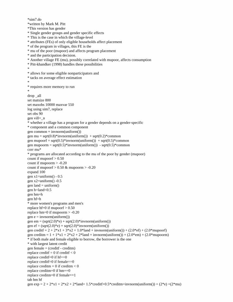
*sim7.do*written by Mark M. Pitt*This version has gender* Single gender groups and gender specific effects* This is the case in which the village-level* attributes (FEs) of only eligible households affect placement* of the program in villages, this FE is the* mu of the poor (mupoor) and affects program placement* and the participation decision.* Another village FE (mu), possibly correlated with mupoor, affects consumption* Pitt-khandker (1998) handles these possibilities* * allows for some eligible nonparticipators and* tacks on average effect estimation** requires more memory to run*drop _allset matsize 800set maxobs 10000 maxvar 550log using sim7, replaceset obs 90gen vill=_n* whether a village has a program for a gender depends on a gender-specific* component and a common componentgen common = invnorm(uniform())gen mu = sqrt(0.8)*invnorm(uniform()) + sqrt(0.2)*commongen mupoorf = sqrt(0.5)*invnorm(uniform()) + sqrt(0.5)*commongen mupoorm = sqrt(0.5)*invnorm(uniform()) - sqrt(0.5)*commoncorr mu** programs are allocated according to the mu of the poor by gender (mupoor)count if mupoorf > 0.50count if mupoorm > -0.20count if mupoorf > 0.50 & mupoorm > -0.20expand 100gen x1=uniform() - 0.5gen x2=uniform() -0.5gen land = uniform()gen h=land<0.5gen hm=hgen hf=h* more women's programs and men'sreplace hf=0 if mupoorf > 0.50replace hm=0 if mupoorm > -0.20gen e = invnorm(uniform())gen em = (sqrt(2.0)*e) + sqrt(2.0)*invnorm(uniform())gen ef = (sqrt(2.0)*e) + sqrt(2.0)*invnorm(uniform())gen creditf = 2 + 2*x1 + 3*x2 + 1.0*land + invnorm(uniform()) + (2.0*ef) + (2.0*mupoorf)gen creditm = 1 + 1*x1 + 2*x2 + 2*land + invnorm(uniform()) + (2.0*em) + (2.0*mupoorm)* if both male and female eligible to borrow, the borrower is the one* with largest latent creditgen female = (creditf - creditm)replace creditf = 0 if creditf < 0replace creditf=0 if hf==0replace creditf=0 if female==0replace creditm = 0 if creditm < 0replace creditm=0 if hm==0replace creditm=0 if female==1tab hm hfgen exp = 2 + 2*x1 + 2*x2 + 2*land+ 1.5*creditf+0.5*creditm+invnorm(uniform()) + (2*e) +(2*mu)

*naive estimatesgen credit = creditm + creditf* naive estimatesregress exp credit x1 x2 landregress exp creditf creditm x1 x2 landgen tf=hf==0gen zfx1=x1*tfgen zfx2=tf*x2gen zfland = land*tfgen tm=hm==0gen zmx1=x1*tmgen zmx2=tm*x2gen zmland = land*tmgen t = (tm==1) | (tf==1)* ignore male female distinctionquietly xi: reg credit x1 x2 land I.vill if hm==1 | hf==1predict pcreplace pc=0 if h==0* two-step with deterministic zero credit for the ineligiblexi: regress exp pc x1 x2 land I.vill* 2sls equivalentxi: regress exp x1 x2 land credit I.vill (x1 x2 land h z* I.vill I.vill*t )* pay attention to male female distinction* note in doing so we allow for different village FEs forboth male and female credit* as in Pitt-Khandker (1998) which handles this exact case of differential* village selection on the basis of the unobserved attributes of the poor (mupoor)quietly xi: reg creditf x1 x2 land I.vill if hf==1predict pcfreplace pcf=0 if hf==0quietly xi: reg creditm x1 x2 land I.vill if hm==1predict pcmreplace pcm=0 if hm==0* two-step with deterministic zero credit for the ineligiblexi: regress exp pcf pcm x1 x2 land I.vill* 2sls equivalentxi: regress exp x1 x2 land creditf creditm I.vill (x1 x2 land h z* I.vill I.vill*tm I.vill*tf )* does not matter if you throw out nonprogram villagesxi: regress exp x1 x2 land creditf creditm I.vill (x1 x2 land h z* I.vill I.vill*tm I.vill*tf ) if mupoorf <=0.50 |mupoorm <= -0.20log close

*sim8.do*written by Mark M. Pitt* Does Morduch's difference-in-the-differences* correctly estimate program effects in a* quasi-experiment?**This is the standard set-up with village FE's* and some eligible nonparticipatorsdrop _allset matsize 400set maxobs 10000 maxvar 300log using sim8, replaceset obs 90gen vill=_ngen mu = invnorm(uniform())count if mu > 0.75expand 100gen x1=uniform() - 0.5gen x2=uniform() - 0.5gen land = uniform()gen h=land<0.5replace h=0 if mu > 0.75* the rich (land > 0.5) in the program village have bigger x's (incl. land)replace x1 = x1 + uniform() + 0.1 if (land > 0.5 & mu < 0.75)replace x2 = x2 + uniform() + 0.1 if (land > 0.5 & mu < 0.75)replace land = 1.25*land if (land > 0.5 & mu < 0.75)gen e = invnorm(uniform())gen credit = 1 + 2*x1 + 2*x2 + 2*land + invnorm(uniform()) + (2.0*e) + (2.0*mu)replace credit = 0 if credit < 0replace credit=0 if h==0gen exp = 2 + 2*x1 + 2*x2 + 2*land + 1*credit+invnorm(uniform()) + (2*e) +(2*mu)* naive estimatereg exp credit x1 x2 land* Pitt-Khandker estimategen t=h==0gen zx1=x1*tgen zx2=t*x2gen zland = land*tquietly xi: reg credit x1 x2 land I.vill if h==1predict pcreplace pc=0 if h==0* two-step with deterministic zero credit for the ineligiblexi: regress exp pc x1 x2 land I.vill* 2sls equivalentxi: regress exp x1 x2 land credit I.vill (x1 x2 land h z* I.vill I.vill*t )* Morduch diffs-in-diffs estimate treating data as experimental*diffs of nonprogram villagesquietly summ exp if mu > 0.75 & land > 0.5scalar npland = _result(3)quietly summ exp if mu > 0.75 & land <= 0.5scalar npless = _result(3)scalar npdiff=npless - nplanddisplay npdiff*diffs of program villagesquietly summ exp if mu < 0.75 & land > 0.5scalar pland = _result(3)quietly summ exp if mu < 0.75 & land <= 0.5scalar pless = _result(3)scalar pdiff = pless - pland*program effects by differencing

display pdiff*program effect by differencing the differencesscalar diffdiff = pdiff - npdiffdisplay diffdiff* Is the above estimate near to the true estimate of +1.0?log close

*sim9.do*written by Mark M. Pitt* Demonstrate that random mistargeting does not necessarily affect consistency* Two-sided mistargeting. Special case of mistargeting "fuzz" orthogonal to the* credit and exp errors.**This is not the argument I rely on in the paper. It is presented simply*to illustrate and interesting special case.**This is the standard set-up with village FE's* and some eligible nonparticipatorsdrop _allset matsize 400set maxobs 10000 maxvar 300log using sim9, replaceset obs 90gen vill=_ngen mu = invnorm(uniform())count if mu > 1.0expand 100gen x1=uniform() - 0.5gen x2=uniform() -0.5gen land = uniform()** fuzzy rule, allows for random mistargeting up to 0.5 acres *** note that landed hh's incorrectly made eligible are more likely to borrow *gen fuzz = 0.5*(uniform() - 0.5)gen h=(land + fuzz) < 0.5replace h=0 if mu > 1.0** count mistargeted households in program villages **gen byte landed = land > 0.5tab h landed if mu < 1.0, row gen e = invnorm(uniform())gen credit = 1 + 2*x1 + 2*x2 + 2*land + invnorm(uniform()) + (2.0*e) + (2.0*mu)replace credit = 0 if credit < 0replace credit=0 if h==0gen exp = 2 + 2*x1 + 2*x2 + 2*land + 1*credit+invnorm(uniform()) + (2*e) +(2*mu)*naive estimatereg exp credit x1 x2 landgen t=h==0gen zx1=x1*tgen zx2=t*x2gen zland = land*tquietly xi: reg credit x1 x2 land I.vill if h==1predict pcreplace pc=0 if h==0* two-step with deterministic zero credit for the ineligiblexi: regress exp pc x1 x2 land I.vill* 2sls equivalentxi: regress exp x1 x2 land credit I.vill (x1 x2 land h z* I.vill I.vill*t )log close

*sim10.do*written by Mark M. Pitt* Demonstrates that random mistargeting does not necessarily affect consistency* One-sided mistargeting. All the landless are eligible* but some of the landed also get in. Special case of mistargeting "fuzz"* orthogonal to credit and exp errors.**This is not the argument I rely on in the paper. It is presented simply*to illustrate and interesting special case.**This is the standard set-up with village FE's* and some eligible nonparticipatorsdrop _allset matsize 400set maxobs 10000 maxvar 300log using sim10, replaceset obs 90gen vill=_ngen mu = invnorm(uniform())count if mu > 1.0expand 100gen x1=uniform() - 0.5gen x2=uniform() -0.5gen land = uniform()** fuzzy rule, allows for one-sided random mistargeting up to 0.5 acres *** note that landed hh's incorrectly made eligible are also more likely to borrow *gen fuzz = 0.5*(uniform() - 0.5)gen h = land <= 0.5replace h=1 if (land + fuzz) < 0.5replace h=0 if mu > 1.0** count mistargeted households in program villages **gen byte landed = land > 0.5tab h landed if mu < 1.0, row gen e = invnorm(uniform())gen credit = 1 + 2*x1 + 2*x2 + 2*land + invnorm(uniform()) + (2.0*e) + (2.0*mu)replace credit = 0 if credit < 0replace credit=0 if h==0gen exp = 2 + 2*x1 + 2*x2 + 2*land + 1*credit+invnorm(uniform()) + (2*e) +(2*mu)*naive estimatereg exp credit x1 x2 landgen t=h==0gen zx1=x1*tgen zx2=t*x2gen zland = land*tquietly xi: reg credit x1 x2 land I.vill if h==1predict pcreplace pc=0 if h==0* two-step with deterministic zero credit for the ineligiblexi: regress exp pc x1 x2 land I.vill* 2sls equivalentxi: regress exp x1 x2 land credit I.vill (x1 x2 land h z* I.vill I.vill*t )log close

*sim13.do*written by Mark M. Pitt* Demonstrate that choice of a high enough break-point* even with non-random mistargeting may still yield consistent* estimates if breakpoint is set high enough* * Two-sided mistargeting**This is the standard set-up with village FE's* and some eligible nonparticipatorsdrop _allset matsize 400set maxobs 10000 maxvar 300log using sim13, replaceset obs 90gen vill=_ngen mu = invnorm(uniform())count if mu > 1.0expand 100gen x1=uniform() - 0.5gen x2=uniform() -0.5gen land = uniform()** fuzzy rule, allows for non-random mistargeting up to 0.3 acres *** note that landed hh's incorrectly made eligible are more likely to borrow *gen fuzz = 0.3*(uniform() - 0.5)gen factor=fuzzreplace factor = 0.0 if fuzz > 0.15replace factor = 0.0 if fuzz < -0.15gen h=(land + fuzz) < 0.5replace h=0 if mu > 1.0** count mistargeted households in program villages **gen byte landed = land > 0.5tab h landed if mu < 1.0, row * fuzz factor affects demand for credit and exp directly through error egen e = 0.75*invnorm(uniform()) + 5*fuzzgen credit = 1 + 2*x1 + 2*x2 + 2*land + invnorm(uniform()) + (2*e) + (2*mu)replace credit = 0 if credit < 0replace credit=0 if h==0gen exp = 2 + 2*x1 + 2*x2 + 2*land + 1*credit+invnorm(uniform()) + (2*e) +(2*mu)*naive estimatereg exp credit x1 x2 land*breakpoint is set to actual fuzzy brekpoint of 0.5*correlated "fuzz" causes bias*gen t=h==0gen t=h==0tab t hgen zx1=x1*tgen zx2=t*x2gen zland = land*t* with breakpoint of 0.5 get bias* use t instead of h belowxi: regress exp x1 x2 land credit I.vill (x1 x2 land t z* I.vill I.vill*t )*now use higher breakpoint to eliminate fuzz error (use 0.65 instead of 0.50)drop t zx1 zx2 zland*gen t=h==0gen t=h==0replace t = 0 if land < 0.65tab t hgen zx1=x1*tgen zx2=t*x2

gen zland = land*t* Pitt-Khandker estimates with high breakpointxi: regress exp x1 x2 land credit I.vill (x1 x2 land t z* I.vill I.vill*t )log close