CA/DOH/AIHL/SP-29·

·i .• ,:

\. ,.

l ; \ J.

' ( ;,

lt I i }

VISIBILITY REDUCTION AS RELATED TO AEROSOL CONSTITUENTS

Interagency Agreement No. ARB A1-081-32

Final Report

October 1983

Prepared by

B. R. Appel, Y. Tokiwa, J. Hau, E. L. Kothny, E. Hahn and J. J. Wesolowski

Air and Industrial Hygiene Laboratory California State Depar~ment of Heal th., Servi~es

2151 ·Berkeley Way , · ·Berkeley Way

.. Ber~~ley, ·· California 94704

Board"\,

iaion. ,·-:·· . . . i:r;- ~~~,?,~~~es

The statements and conclusions in this re-port are those of the Contractor

and not necessarily those of the State Air Resources Board. The mention of

commercial products, their source or their use in connection with material

re-ported herein is not to be construed as either an actual or implied

endorsement of such products.

- 2 -

ABSTRACT

A laboratory and field study was performed to assess the contribution to

visibility reduction of both light-scattering and absorJ)tion by air

pollutant particles and gases. Gaseous precursors to important visibility­

reducing aerosol species were measured. Emphasis was placed on minimizing

sampling artifacts for nitrate and sulfate since ~revious visibility studies

were generally subject to substantial errors from these sources. Optical

techniques for measuring the particle absorption coefficient and elemental

carbon were evaluated. The aerosol species measured were fine and coarse

particulate mass, sulfate, nitrate, and elemental carbon, plus organic

carbon and ammonium ion. The gases measured were nitric acid, NH 3, so 2,

N02, and 03. Sampling was done at San Jose, Riverside and downtown

Los Angeles.

At all sites light scattering by sulfate, nitrate and elemental carbon

particles contributed more than half of the light extinction. Light

absorption by ~articles, due almost ex c 1 us i ve ly to e 1 emen ta 1 carbon,

contributed 10 to 20% of the extinction. The light-scattering efficiency of

fine particulate nitrate appeared to be higher than that of sulfate, in

contrast to the findings of most prior studies.

- 3 -

ACKNOWLEDGEMENT

We wish to acknowledge the assistance of Vincent Ling who performed many of

the carbon determinations and aided in data analysis. Meyer Haik also

performed carbon determinations. SuzAnne Twiss supervised the multiple

regression analysis of the data. Dr. Allen Waggoner, University of

Washington, provided the modified integrating nephelometers together with

detailed instructions and advice on their calibration and use. Dr. Ray

Weiss, University of Washington, provided valuable comments and aid in

setting up and com-paring results for the integrating plate method. Dr.

Stephen Cadle, General Motors Research Laboratory, provided analyses

permitting interlaboratory comparison of our procedures for elemental carbon

measurement. Drs. T. Novakov, H. Rosen, A. Hansen and L. Gundel, University

of California, Lawrence Berkeley Laboratory, provided information on the

design of their laser transmission method, samples for interlaboratory

comparison, and useful discussions. Dr. John Trijonis provided many

valuable comments on the final report.

Sampling sitea .were furnished by Professor Kenneth MacKay, San Jose State

University, Dr. Arthur Winer, University of California, Riverside, and Mr.

Frank Baumann, Southern California Branch Laboratory Section, Laboratory

Services Branch, California Department of Health Services.

Finally, we acknowledge Dr. Douglas Lawson and Dr. John Holmes, Air

Resources Board Research Division, for their helpfulness and sup-port

throughout this program.

This report was submitted in fullfillment· of Interagency Agreement No. A1-

081-32, Visibility Reduction as Related to Aerosol Constituents by the

California De-partment of Heal th Services under the sponsorship of the

California Air Resources Board. Work was completed as of November 10, 1983.

- 4 -

TABLE OF CONTENTS

Abstract Acknowledgements List of Figures List of Tables

I. Summary and Conclusions 12

II. Introduction

A. Visibility and its Relation to Aerosol Constituents............. 17

B. Limitations of Prior Studies.................................... 20

C. Objectives of the Present Study................................. 24

D. Strategy........................................................ 24

III. Measurement of the Particle Absorption Coefficient (b )ap

A. The Integrating Plate Method (IPM).............................. 26

B. A Laser Transmission Method (LTM).............................. 29

c. Comparison of B ap Determinations by the IPM and LTM............. 30

IV. Determination of Elemental Carbon (C)e

A. Introduction • • • • • • • • • • • • • • • • • • • • • • • • • • • • • • • • • • • • • • • • • • • • • • • • • • • • 32

B. The Laser Transmission Method for Ce ••·•••·····•···••··•·•·•·•··• 32

C. Intermethod and Interlaboratory Comparisons..................... 33

D. Comparison of C by Optical Methods with Particle Absorption Coifficient Results •••••••••••••••••••••••••••••••••• 35

v. Measurement of the Scattering Coefficient for Liquid Water

A. Introduction • • • • • • • • • • • • • • • • • • • • • • • • • • • • • • • • • • • • • • • • • • • • • • • • • • • 37

B. Method Evaluation and Correlation with Aerosol Constituents..... TI

VI. Assessment of Sampling Artifacts

A. Artifact ~articulate Sulfate on Glass Fiber Filters............. 39

- 5 -

B. Artifact Particulate Nitrate on Glass Fiber Filters............ 39

c. Loss of Particles in the Denuder of the Particulate Nitrate (PN) Sampler. • • • • • • • • • • • • • • • • • • • • • • • • • • • • • • • • • • • • • • • • • • • • • • • • • 40

D. Loss of Non-Volatile Carbon in the Denuder of the ?articulate Carbon Sam-pler. • • • • • • • • • • • • • • • • • • • • • • • • • • • • • • • • • • • • • • • • • • • • • • • 41

E. Retention of Carbonaceous Material on Hi-Vol Filter Samples..... 41

VII. Atmospheric Results -- Part I.

A. Tabulation of Results........................................... 42

B. Summary of Visibility Results................................... 42

c. Diurnal Variation of the Dominant Aerosol Species and Ozone..... 43

D. Size Distribution for Aerosol Constituents...................... 43

E. Calculated vs. Observed Ammonium. Ion Levels..................... 45

F. True Particulate Carbon (PC) and Total Low Volatility Carbon (LVC).................................................. 46

G. Atmospheric Nitric Acid......................................... 46

VIII. Atmospheric Results -- Part II. Statistical Analyses

A. Correlation between Pollutant Concentrations.................... 48

B. Correlation between Single Pollutant Concentrations and Visibility Parameters......................................... 48

C. Multiple Regression Analyses between Particle Scattering Coefficients and Pollutant Concentrations •••••••••••• 49

D. Average Contributions of Aerosol Species to the Scattering and Total Extinction Coefficients. • • • • • • • • • • • • • • • • • • • • • • • • • • • • • • • • 51

E. Comparison of Present Results with those for General Motor's Denver Visibility Study....................................... 52

F. Comparison of the Present Results to those Reported by Trijonis et al( 48) •••••••••••••••••••••••••••·••••••••••••••••• 53

- 6 -

IX. References

Appendices

A. The Impact of Increased Diesel Emissions on Visibility......... 62

B. Operation of the Integrating Nephelometers..................... 65

C. Evaluation of Methods for Absorption Coefficient Measurement... 66

D. Calibration of Optical Methods for Elemental Carbon............ 79

E. Measurement of Ambient Temperature and Relative Humidity....... 85

F. Experimental Difficulties with the True Particulate Carbon Measurements.......................................... 86

- 7 -

FIGURES

Number

1. Light Scattering by Aerosols as a Function of Particle Diameter Com~uted for Unit Density Spherical Particles of Refractive Index 1.5.......... 19a

2. Schematic of Integrating Plate Method (IPM)............................. 26a

Comparison of b Measurements at Two Particle Loadings ••••••••••••••••• 28a ap

Comparison of the Integrating Plate Method and Laser Transmission Techniques for Absorption Coefficient Measurement ••••••••••••••••••••• 29a

5. Schematic Diagram of Laser Transmission Method, Viewed From Above ••••••• 30a

6. Comparison of b Measurements by the IPM and LTM Methods ••••••••••••••• 30b ap

Elemental Carbon by the LTM vs. Reflectance Method•••••••••••••••••••••• 34a

8. Relation between Absorption Coefficient and C for Denver Winter Aerosol 35a e

9. Elemental Carbon by LTM vs. Absorption Coefficients..................... 35b

10. Elemental Carbon by the RM vs. Absorption Coefficients.................. 35c

11. Mean Elemental Carbon by LTM and RM vs. Absorption Coefficients......... 35d

12. Artifact Sulfate on Glass Fiber Filters, 4-hour Hi-Vol Samples.......... 39a

13. Nitric Acid Retention on Glass Fiber Hi-Vol Filters ••••••••••••••••••••• 40a

14. Nitric Acid Retention of Glass Fiber Hi-Vol filters ••••••••••••••••••••• 40b

15. Nitric Acid Retention of Glass Fiber Hi-Vol Filters ••••••••••••••••••••• 40c

16. Nitric Acid Retention of Glass Fiber Hi-Vol Filters ••••••••••••••••••••• 40d

17. Loss of Non-Volatile 'Particles in the Denuder for Nitrate Sampling •••••• 40e

18. Loss of ton-Volatile Particles in the Denuder of the Particulate Carbon Sampler. • • • • • • • • • • • • • • • • • • • • • • • • • • • • • • • • • • • • • • • • • • • • • • • • • • • • • • • 41 a

19. Observed vs. Calculated 16-hour Total Carbon............................ 41b

20. Mass Comparisons 1982 ARB Visibility Study.............................. 43a

21. Comparison of Fine and Total Particulate Sulfate........................ 43b

22. Comparison of Fine and Total Particulate Elemental Carbon............... 43c

23. Fine Elemental Carbon vs. Total Carbon in 4-hour Samples................ 43d

- 8 -

Number Page

24. Fine Particle Mass vs. Fine Particle Elemental Carbon••••••••••••••••••••• 43e

25. Total Particle Mass. vs. Fine Particle Elemental Carbon•••••••••••••••••••• 43f

26. Comparison of Filter Collected Carbon with and without a Diffusion Denuder for Carbonaceous Vapors ••••••••••••••••••••••••••••••••••••••••••••••••• 43g

'Z7. B Values San Jose••••••••••••••••••••••••••••••••••••••••••••••••••••••••• 44a

28. B Values Riverside •••••••••••••••••••••••••••••••••••••••••••••••••••••••• 45a

29. B values Los Angeles •••••••••••••••••••••••••••••••••••••••••••••••••••••• 45b

30. Diurnal Variations in Mean Pollutant Concentrations (San Jose) •••••••••••• 45c

31. Diurnal Variations in Mean Pollutant Concentrations (Riverside) ••••••••••• 45d

32. Diurnal Variations in Mean Pollutant Concentrations (Los Angeles) ••••••••• 46a

Scatter Diagram of Fine Particulate Mass Against the Dry Particle Scattering Coefficient ••••••••••••••••••••••••••••••••••••••••••••••••••

34. Comparison of Calculated and Observed b' ext•••···•··•··•··•···········••·· 51a

C-1. Linearity of LTM Detector Response •••••••••••••••••••••••••••••••••••••••• 74a

C-2. Comparison of AIHL and Lawrence Berkeley Laboratory LTM Instruments Analyzing the Same Atmospheric Particulate-loaded Millipore Filters ••••• 76a

D-1. Size distribution for Aged Carbon Particles from a Butane Flame ••••••••••• 80a

D-2. Calibration of LTM with Aged Carbon Particles ••••••••••••••••••••••••••••• 80b

D-3. Calibration of LTM with LBL Black Carbon Samples •••••••••••••••••••••••••• 81a

D-4. Light Absorption Efficiency for Graphitic Carbon•••••••••••••••••••••••••• 81b

D-5. Calibration of Reflectance Meter with Aged Carbon Particle Samples •••••••• 82a

D-6. Calibration of Reflectance Meter with Aged Carbon Particle and LBL Black Carbon Samples •••••••••••••••••••••••••••••••••••••••••••••••••••••• ~ ••• 82b

E-1. Temperature Comparisons 1982 ARB Visibility Study••••••••••••••••••••••••• 85a

E-2. RH Comparisons 1982 ARB Visibility Study•••••••••••••••••••••••••••••••••• 85b

- 9 -

TABLES

Number

Summary of Extinction Coefficients per Unit Mass Obtained in Various Regression Studies •••••••••••••••••••••••••• 18a

2 Contribution of the Chemical Species to the Extinction Coefficient, for Denver••••••••••.•••••••••••..•.••••.•• 21a

3 Description of Samplers Employed for Visibility Study •••• 25a

4 .Analytical Strategy for Visibility Study ••••••••••••••••• 25c

5 Calibrations of Optical Methods for Elemental Carbon ••••• 33a

6 Comparison of Total Carbon and Elemental Carbon (C) Values ( JJg/m3) ••••••••••••••••••••••••••••••••• ~ ••••••• 33b

7 Comparison of Elemental Carbon Measurements by General Motors' Combustion and AIHL Optical Methods ••••••••••• 34b

8 Pearson Correlation Coefficients Between b , Pollutant and Meteorological Parameters •••••••••• ~~ •••••••••••••• Tia

9 Multiple Regression Analysis Between b w and Aerosol 8Constituents ••••••••••••••••••••••••••••••••••••••••••• 38a

10 Summary of Atmospheric Results ••••••••••••••••••••••••••• 42a

11 Explanation of Headings Used in Table 10 ••••••••••••••••• 42c

12

13

Mean Concentrations of Aerosol Constituents and Meteorological Parameters ·········••••···••··•·····•··•

Summary of Optical Measurements at San Jose, Riverside and Los Angeles ••••••••••••••••••••••••••••••

42d

42e

14 Pearson Correlation Coefficients Between Aerosol Constituents Ozone and Meterological Parameters 48a

15

16

Correlation Between Fine Aerosol Constituents (or Aerosol Precursors) and b ••••••••••••••••••••••••• sp

Pearson Correlation Coefficients Between Visibility Parameters, Individual Pollutants and Meterological Parameters •••••••••••••••••••••••••••••••

48b

48c

- 10 -

Number

17

18

Multiple Regression Analysis Between Aerosol Constituents and b ••••••••••••••••••••••••••••••••••• sp

Average Percent Contributions of Chemical Species to the Particle Scattering Coefficient, b and to the Extinction Coefficient, b' t •••• ~Y............... . ex

50a.

52a

C-1

C-2

Precision of Parallel Sampling for b Measurement ••••••• ap

Effect on Transmittance of Overlaying Loaded Nuclepore Filter with a Microsco~e Slide •••••••••••••••••••••••••

68a

69a

C-3 Effect of Neutral Density Filter on t T of Loaded Filters ·•·••••··•••••·•··•···••·······•·······•• 70a

C-4 Effect of Particle Orientation on% T •••••••••••••••••••• 71a

C-5 Interlaboratory Comparison of IPM (% T) •••••••··••••••••• 72a

C-6 Batch-to-Batch Variations in Mean Transmittance Values for 0.4 um Pore Size Nuclepore Filters ••••••••••••••••• 73a

C-7 Influence of Particle Orientation with the IPM and LTM •••••••••••••••••••••••••••••••••••••••••••••••• 76b

C-8 Influence of Wavelength and the Discrepancy Between the IPM and LTM Methods •••••••••••••••••••••••••••••••• 78a

D-1 Size Distribution for Carbon Particles ••••••••••••••••••• 79a

- 11 -

I.· SID.i!MARY AND CONCLUSIONS

A laboratory and field study was performed to assess the contribution

to visibility reduction at both light-scattering and absorption by air

pollutant -particles and gases. Gaseous precursors to important

visibility-reducing aerosol species were also measured. Em-phasis was

placed on minimizing sampling artifacts for pollutant particles since

preceding visibility studies were generally subject to substantial

errors from this source. 0-ptical techniques to measure the particle

absorption coefficient and elemental carbon were evaluated.

The aerosol species measured were fine and coarse particulate sulfate,

nitrate, elemental carbon and mass. In addition, total pa rt i culate

o rg a ni c carbon and ammonium ion were determined. The gases measured

were nitric acid, NH3, S0 2 , N0 2 and o3• Artifact sulfate formation was

minimized by using Teflon filters. Particulate nitrate and nitric acid

were measured using the denuder difference technique. Particulate

organic carbon was sampled with two conventional hi-vol samplers with

glass fib.er filters, providing both 4-hour and 16 to 24 hr samples. In

addition, a- diffusion denuder plus a quartz filter and a fluidized

Al 2o3 bed were used in an effort to determine particulate carbon whi 1 e

minimizing both positive and negative sampling errors. However,

ex-perimental difficulties prevented the development of useful data from

this sampler.

The particle absorption coefficient was measured by the integrating

plate method using two samplers operating at different particle

loading rates. 'fillemental carbon was measured optically by both a

reflectance method and by a method which measured the absorption of a

He-Ne laser beam. Two integrating nephelometers operated side-by-side

to measure light-scattering by particles with and without heating the

incoming air. The difference in results between these instruments was

used to approximate light-scattering due to liquid water.

- 12 -

Sampling was done for a total of 109, 4-hour periods, generally between

0800 and 2400 hours, July 10 - August 8, 1982, at San Jose, Riverside

and downtown Los Angeles. The mean visual range encountered, as

estimated from the calculated extinction coefficients and the

Koschmeider equation, were 43 Km at San Jose, 15 Km at Riverside and 13

Km at downtown Los Angeles. The mean four-hour average ozone

concentrations ranged from 0.02 to 0.(17 ppm. Thus relatively light

photochemical smog was experienced.

Light scattering by dry particles was the largest contributor to the

total extinction (b' t) at all sites, representing more than half of ex

the extinction coefficient. Light absorption by particles, due almost

exclusively to elemental carbon, was relatively unimportant (.s_ 12% of

b' t) in the South Coast Air 'Basin where high concentrations of ex

sulfate and nitrate were present. At San Jose, however, absorption

averaged nearly 22% of b' t· The apparent contribution of scatteringex

from liquid water was relatively high at Riverside and Los Angeles but

small at San Jose, paralleling the concentrations of the hygroscopic

aerosol species, sulfate and nitrate. Light absorption· by gases, due

only to N0 2 , was small at all sites.

Considering both light scattering and light absorption, and using

multiple regression analysis, fine sulfate and fine nitrate (and

associated water), fine elemental carbon, and nitrogen dioxide

contributed on average, 30%, 36%, 20%, and 8%, respectively, to the

total extinction (excluding Rayleigh scattering).

Sulfate, nitrate, elemental carbon, and total carbon were predominately

in the fine ( < 2. 5 µm) fraction averaging 92%, 60%, 80%, and 62%

respectively, measured by comparing results with and without a cyclone

preceding the sampler. The percentage of fine total carbon can be

compared to the range 56 to 66% previously obtained at three sites

using a dichotomous sampler (DS). We previously suggested that the

proportion of coarse particle carbon with a DS ma.y be erroneously high

- l3 -

because of the low face velocitv for the coarse narticle filter

(34,40). The nresent data fail to su-pnort this.

Multinle regression analyses between the drv particle scattering

coefficient and aerosol s~ecies concentrations vielded the

relationshin:

where F = fine

C • coarse

Tlms the scattering efficiency per unit mass of nitrate apl)ears to be

greater than that for fine sulfate, in contrast to most -previous

studies. The scattering efficiency for fine elemental carbon (C )e

was

similar to that for fine sulfate. The results for coarse sulfate are

surprising, iml)lying a scattering efficiency twice that for fine

sulfate. We believe that some material whose concentration is much

higher but pro-portional to that of coarse sulfate is the actual

scattering source. Sea salt chloride, for example, is about seven

times the weight concentration of sea salt sulfate. A significant

amount of sea salt would be ex1'ected in the coarse fraction. Re~lacing

the coarse sulfate concentration with a material seven times more

abundant would decrease the scattering efficiencv per unit mass by an 4 1

equal factor of seven (i.e. to< 0.02 x 10- m- /~g/m3). The remaining

aerosol species, coarse nitrate, coarse elemental carbon, and organic

carbon, did not exhibit a significant scattering efficiency in this

evaluation.

Multi~le regression analyses between the measured scattering

coefficient for liquid water and the concentrations of the hy'grosco-pic

aerosol s-pecies S0 4= and N03-, using various functions of relative

humidity, showed only moderate correlation (r i 0.81). This may be

- l4 -

indicative of lack of speciation data for sulfate since, for example,

H zSO 4 and ( 'f\'.JH 4 ) 2SO 4 differ substantially in hygroscopici ty. It may

also indicate error in measuring the scattering coefficient for liquid

water, since species other than liquid water may be volatilized on

entering a heated nephelometer inlet (e.g. organic comuounds, 'tifH 4N03).

Artifact particulate nitrate formation on ~lass fiber filters (prefired

Schleicher and Schuell, 1qs1 EPA Grade) was assessed for both 4-hour

and 16-hour atmospheric samples. With the short-term samples,

essentially all particulate nitrate and nitric acid was retained,

supporting the use of glass fiber as total inor~anic nitrate (TI'tll)

collectors. With the long-term sam'!)les, however, onlv at low nitrate

levels such as found at San Jose ( TIN i '32 iag/cm2) was all TIN

retained; at Riverside and Los Angeles with 't'IN values up to 147

µg/cm 2 , from 24 to 42% of the TIN ~enetrated the filters, presumably as

HNO 3.

Expected HN03 concentrations can be calculated from the concentration

of NH 3, temperature, and corresponding dissociation constant for

In general, no correlation between the observed and expected

HN03 levels was found. Similarily, the correlation between NH 3 or HN0 3

and the particle scattering coefficient remained relatively low.

The principal conclusions from this study are:

1. The light-scattering efficiency of fine particle nitrate appears to

exceed that of sulfate in contrast to most previous studies. Since

both positive and negative sampling artifacts were minimized we

believe these results to be correct.

2. Light absor-ption by elemental carbon plays a significant role in

visibility reduction in California, especially under conditions in

which the concentrations of fine sulfate and nitrate are relatively

low.

- 15 -

3. Particle--phase water contributed substantially to visibility

reduction at sites with relatively high levels of sulfate and

nitrate, species which can absorb moisture.

Recommendations for Further Studies

1., The significance of true particle phase organic com-pounds in visibility

reduction. Although organic carbon, based on hi-vol filter sampling, was

not a statistically significant contributor to visibility reduction,

sampling errors may have masked such a contribution.

2. The a c curacy of elemental carbon measurement by optical methods. While

the elemental carbon measurements reported are consistent with other

o-ptical measurements, calibration techniques for elemental carbon

measurements by optical methods require more work before their adoption

for routine monitoring of elemental carbon can be recommended.

3. The relative significance of aerosol constituents in visibility reduction

using the same.techniques at other times of the year.

4. Additional statistical analysis of results from the present study to

a) assess the significance of the aerosol and gaseous pollutants to

visibility reduction by site, b) assess the hypothesis that coarse sulfate

is functioning as a surrogate for sea salt, and c) assess the impact of

co-linearity of variable.

- 16 -

II. INTRODUCTION

A. Visibility and Its Relation to Aerosol Constituents

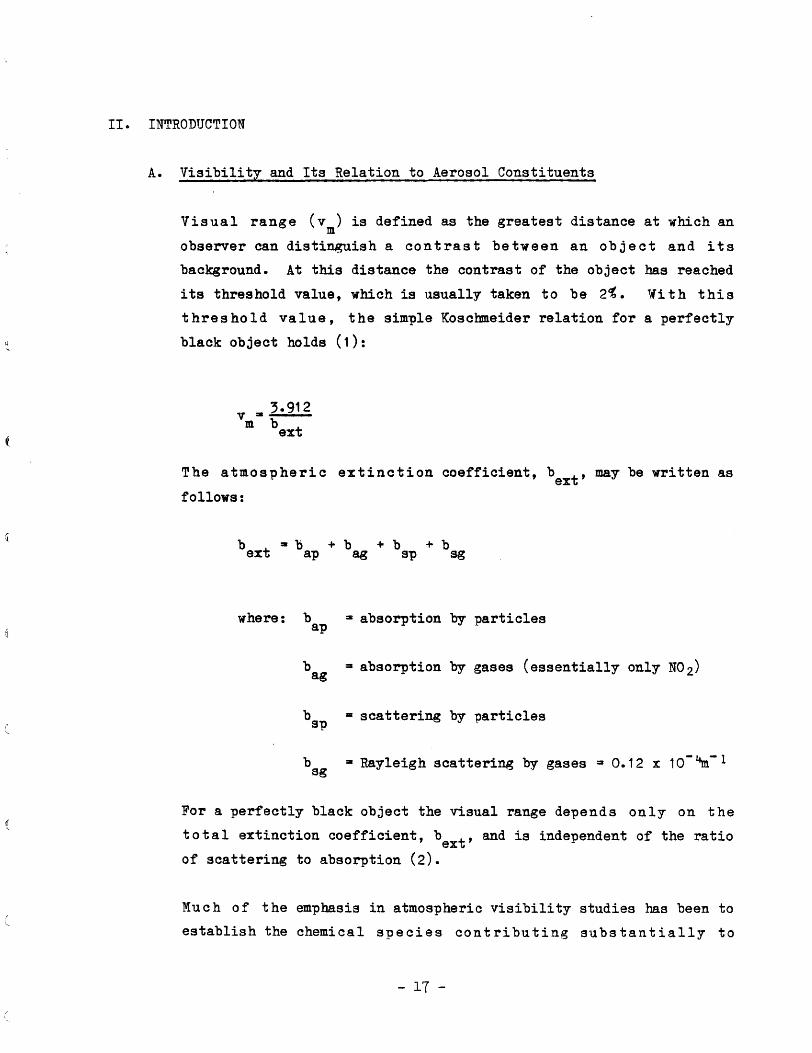
Visual range ( v ) is defined as the greatest distance at which an m

observer can distinguish a contrast between an object and its

background. At this distance the contrast of the object has reached

its threshold value, which is usually taken to be 2~. With this

threshold value, the simple Koschmeider relation for a perfectly

black object holds (1):

3.912 V :a -------

m bext

The atmospheric extinction coefficient, bext' may be written as

follows:

b =- b + b + b + bext ap ag sp sg

where: b = absorption by particlesap

b ag

= absorption by gases (essentially only N0 2)

b • scattering by particlesSl)

b = Rayleigh scattering by gases= 0.12 x 10_1io._ 1 sg

For a perfectly black object the visual range depends only on the iz

total extinction coefficient, b t' and is independent of the ratio ex of scattering to absorption (2).

Much of the emphasis in atmospheric visibility studies has been to

establish the chemical spa cies cont ri bu ting substantially to

- 17 -

visibility reduction (3-8). Typically b tis approximated by b , ex s~

as measured by the integra.ting nephelometer or as approximated from

human observer data. Indeed, b will often represent more than 2/3Sp of the total extinction coefficient. Multiple regression analyses

are performed with equations of the form:

= -where R = Remaining aerosol = TSP - SO 4 - NO 3

RH a relative humidity

Relative humidity de-pendence may, alternatively, be incorporated

into the sulfate and nitrate terms. In the cases where data on

carbonaceous material are available, additional terms [e.g.

b (benzene soluble organics)] a.re added.5

Table 1, taken from a recent survey by Trijonis,(3) summarizes the

scattering coefficients per unit mass for a series of visibility

studies. Princi-pal conclusions that ca.n be reached from these

studies ~re:

1. Sulfates, per unit mass, are the dominant contributor to

visibility reduction due to light scattering.

2. Nitrates, -per unit mass, can be an important contributor to

visibility reduction due to scattering. However, in locations

not dominated by photochemical smog, their contribution will be

relatively small because of the low nitrate levels.

The contribution of relative humidity as well as organics is

illustrated with results from a study by Hidy et al.: (4)

- 18 -

TABLE 1

LOCATION

SUMMARY OF EXTINCTION COEFFICIENTS PER UNIT MASS OBTAINED IN VARIOUS REGRESSION STUDIES.

(From Trijonis et al. Reference 3)

Locations in California.

Other Studies SOUTH COAST AIR BAS IN (White and Roberts 1977)Various Los Angeles Basin Sitest

(Cass 1979)Downtown Los Angeles

(Grosjean et al. 1976) Eastern Los Angeles Basin

(Leaderer and Stolwijk 1979)Los Angeles Int. Airport

The Present Study SOUTH COAST AIR BASIN Burbank

Long Beach

Ontario

t San Bernardino

SAN FRANCISCO BAY AREA AIR BASIN Oakland

San Jose

OTHER COASTAL LOCATIONS Paso Robles

San Diego

SAN JOAQUrn VALLEY AIR BASIN Bakersfield

Fresno

SACRAMENTO VALLEY AIR 8J\SIN Red Bluff

Sacramento

*Values marked by an asterisk are

EXTINCTION COEFFIC!EtlTS PER U~IIT M.il.SS (104 m)-l/(µg/m3)

Sulfates rlitrates Remainder of TSP

.01. .as. .015,.

.06 .04 .020

.11. NS. .008

.09 .OS NS*

.21 .04 ~,s

.16 .03 NS

•17. ~•s• · NS .., .15 NS .008

.16. .04* .011.,..

.11 • NS .013

•16,. .1s • r~s. .17 .11 NS

.12,. NS,. .019..,

.06 .OS .019

.12 .. NS,. .014.

.08 NS .014

NS* .06.., NS* NS .04 NS

.08.,, Dos* .008.,,

.,06 .as .006

.19. .04.,,, NS,.

.15 .OS NS

NS* .09. NS* NS .07 NS

NS.., 014* ~lS.,. M$ .07 HS

~s. .03* .009.,,, NS .04 .008

•16* .as• .014* .15 .03 .014

based on the nonlinear RH regression model with insertion of average RH. Va1ues not so marked ~re based on the J;near RH model.

tBased on nephelometry data rather than airport visibility data.

- lBa-

TABLE 1 SUMMARY OF EXTINCTION COEFFICIENTS PER UNIT MASS OBTAINED IN VARIOUS REGRESSION STUDIES (Continued).

(From Trijonis et al. Reference 3)

Locations in the ~ortheast and Rocky~ountain Southwest.

EXTINCTION COEFF!C IENTS PER U1'1IT MASS (104 m)-l/(~g/rn3)

LOCATION Sulfates ~Ii tra tes Remainder of TSP

NORTliEAST

(Trijonis and Yuan, 1978b) Chicago .04..,

.03 NS,. NS

NS* NS

Newark NS.., NS,. .026* .06 NS .014

Cleveland .08 NS* NS* .07 tlS NS

Lexington .06. .06

NS* NS

NS* .019

Charlotte. .11... NS* NS* .11 t4S NS

Columbus .12... .09. NS* .13 .06 NS.

(Leaderer and Stolwijk 1919) Ne•,., Yorkt .07 .OS NS

New York .10 NS NS

New Haven .16 NS- NS

St. Louis .08 NS NS

ROCKY MOUNTAIN SOUTHWEST

(Trijonis 1979)

Phoenix County Data NASN Data

.04

.03 .OS .OJ

NS NS

Salt Lake City .04* .04

•13,. .10

.004...

.004

*1/alues marked by an asterisk are based on the nonlinear RH regression Model ~ith insertion of average RH. Values not so marked are based on the linear RH model.

tBased on nephelometry d~ta rather than airport visib11ity data.

- 18b-

+ 0.025(total carbon) + 0.025(R)

RHwhereµ a 1 - 100

Ra remaining aerosol a TSP - S04 a

- N03- - total carbon

Some studies have incorporated relative humidity-dependent

sulfate terms as well (3,7).

The dominance of sulfate in contributing to light sea ttering

and the influence of relative humidity on light scattering can

be interpreted in relation to 'Figure 1. Growth caused by­

pickup of water would be expected to enhance light scattering

for sulfate particles initially smaller than 0.5 µmin

diameter, since scattering efficiency exhibits a sharp maximum

at 0.5 lJDl• Sulfates in various urban areas around the United

States have been reported to have mass median diameters (mmd)

ranging from 0.1 to 0.6 lJDl (9). Nitrate mass median diameters

are much more varied. In California's South Coast Basin, 24-

hour mean values from 0.3 to 1.6 µm have been reported ( 9),

probably reflecting the proportions of fine mf4N0 3 and coarse

NaN03. Assuming a size distribution for NH~03 similar to that

for particulate sulfate, increasing relative humidity would

increase· the scattering efficiency for this material as well.

The limited data on carbonaceous particules suggest mean

diameters of several tenths of a micrometer. For example, mmd

values of about 0. 3 µm were found for both organic and

elemental carbon in Denver (38). This together with their low

hygroscopicity may explain their lesser scattering efficiency.

- 19 -

0 1 I I I I I J I I I I I I • . 03 .05 .07 0.1 0.2 0.3 0.5 o.7 1.0 2.0 3.0 5.0 7.0 10.0

Cl 0

·r-f

~ S... -f-l .10Cl (1) C) Cl 0

CJ en ,..... .08 ~ CV)

~ ~ bl}

~ 3-c:: '-.... .06 p r--f

IH ,-... (1) a ~ ~

0 ...., bD ,_,. .04"° c:: ""-../'11 •r-f

H (1) -f-l

~ t) .02 r/l

-f-l ..c:: bD

·r-f ~

Particle Diameter (pm)

Figure lo LIGHT SCATTERING BY AEROSOLS AS A FUNCTION OF PARTICLE DIAMETER. COMPUTED FOR UNIT DENSITY SPHERICAL PARTICLES OF REFRACTIVE INDEX lo5 (White and Roberts 1977)

B. Limitations of Prior Studies

1., Most -prior studies have neglected consideration of light

absorption by aerosol constituents.

f

f

2.. Studies based on visual range measurements obtained by a

human observer yield daytime visibility at one or two times

per day. Attempts to correlate these results with 24-hour

average -particulate sampling results (e.g. Ref. 7) are

subject to substantial error since -particulate loadings

will generally be higher during daytime hours.

(

3. Aerosol samples have ty-pically been collected on filters

subject to sampling errors. These include artifact

particulate sulfate and nitrate em-ploying glass fiber

filters, artifact -particulate nitrate for those using

cellulose ester filters, loss of -particulate nitrate

("negative artifact") from inert filters (e.g. Teflon), and

positive and negative artifacts with organics common to all

studies using filter sampling.

4. The aerosol species

limited in number.

measured were generally relatively

a. Artifact Particulate Sulfate (16,17,18)

Artifact particulate sulfate results from -partial

retention of S02 on filters and can yield, with 24-hour

atmospheric samples, errors in the range 3 to 6 ug /m 3 •

To illustrate the potential effect of this error, the

NASN annual geometric mean sulfate value for down town

Los Angeles in 1974 was s.4 ug/m 3 • A -positive error of

4 ug/m 3 in this value would renresent about a 50t

error. The coefficient for the contribution of sulfate

- 20 -

to b would be expected to be too low by an equalSp

percentage. Perhaps more significant, the variability

introduced into sulfate measurements can decrease the

correlation with visibility parameters.

The importance of submicron aerosols in visibility

reduction by light scattering leads to the desirability

of size-segregated particle sampling in visibility­

aerosol chemistry correlation studies.

Recent visibility studies have considered more than

particle scattering contributions. In urban areas the

particle absorption coefficient, due primarily to

graphitic carbon, can contribute substantially to b t ex

(6,12-14). For example Groblicki et al. (Table 2)

reported a mean contribution to b t of 31% due to ex

light absorption by particulate carbon for 41 days of

sampling in Denver ( 6). The contribution of light

absorption by particles to the total extinction

coefficients in California urban areas has only

recently been reported (58).

In Denver the dominant source of atmospheric graphitic

carbon was concluded to be from the combustion of wood.

However, in California urban areas, mobile source

emissions, especially from diesel-powered trucks, are

the predominant source of graphitic carbon. The

increasing use of diesel-powered passenger cars may

serve to increase this source of light extinction.

General Motors has estimated that by the year 2000, 25%

of all passenger vehicles will be diesel-powered (15).

A simple calculation (Appendix A) permits estimation of

a > 12% decrease in mean visual range in downtown Los

Angeles by the year 2000, relative to the 1974-1 976 ! i I ~ /1

- 21 -

11

TABLE 2 CONTRIBUTION OF THE CHEMICAL SPECIES TO THE EXTINCTION COEFFICIENT, FOR DENVER (NOVEMBER - DECEMBER 1978)a

Fine Particulate Species Mean% Contribution

20.2(NHt+) 2S0 t+ and associated H20

NHt+NO 3 and associated H2O 17.2

Organic C 12.5

Elemental C (scattering)

Elemental C (absorption)

Elemental C (total) 37 .7b

Remainder fine particulate 6.6

-2.:1.. TOTAL 1oo.

a. Data of P. J. Groblicki et al., Reference 6.

b. Includes fine and coarse particulate C • e

- 21a -

mean (7. 5 miles), due only to

in gra-phitic carbon, assuming

emissions.

the associated increase

no controls on such

If used for short-term sampling, glass fiber filters

would vield substantially greater artifact· sulfate,

expressed in µg/m3.

b. Nitrate Sampling Errors

(

Artifact -particulate nitrate results from retention of

gaseous HN03. Under atmos-pheric conditions,

and with 4-hour samples, essentially all HNO 3 is

retained by glass fiber filters resulting in errors

which can re-present 50% of the observed nitrate ( 21 ) •

As a result, the corresponding nitrate coefficient in

regression equations with visibility parameters may be

too low by a factor of about two. Similarly, in short

term sampling with cellulose aceta.te filters, 12%

retention for HNO 3 was observed (20) leading. to a

corresponding negative error in the nitrate coefficient

in correlations with visibility.* Studies employing

inert filters (e.g. Teflon) vield nitrate

concentrations which are lower limits to the true

particulate nitrate values because of com-plete

penetration of HN0 3 , and the possibility of nitrate

loss by volatilization and reaction with strong acid

particles (e.g. H2S0 4 ) and gases (e.g. l-ICl) (21-2'3).

In such cases the nitrate coefficients in the

visibility re~ression equation would be ex-pected to be

*As with sulfate,

affected.

the coefficient for the remaining aerosol term is also

- 22 -

too high by an amount which depends on meteorological

variables and concentrations of airborne acids.

In addition to altering coefficients, the variability

in the re lationshi-p between true particle nitrate and

that measured by simple filter methods can severely

decrease correlation coefficients with visibility

parameters.

c. Organic Particle Sampling Errors (24-34, 63)

Of the major classes of aerosol constituents least is

known about the errors in sampling organics. Many of

the organic materials retained on a filter exist in the

gas phase as well. The proportion in each phase

in the atmos-phere probably varies with atmos-pheric

conditions (e . .g. temperature and R.H.), the

concentration of the pollutants. The contribution of

organics to visibi li ty reduction should reflect the

fraction of the organics in the particle -phase at any

moment. Following collection on a filter, volatile

organics may be lost depending on the degree of

saturation of the air stream with each organic

compound. As an opposing source of error, gas -phase

organics may be retained by sorption on previously

collected particulate constituents and on the f i 1 t er

medium. As a result, neither the ma~nitude nor

direction of the ·error can be estimated without

specific measurements.

As with sulfate and nitrate, the variability introduced

in f i 1 t er sampling of organic -particles will probably

decrease or eliminate correlations with visibility

parameters.

- 23 -

c. Objectives of the Present Study

1. To assess the contribution to visibility reduction of light

scattering and absorption by specific pollutant -particles and

gases, measuring the aerosol s-pecies with minimum sampling

artifacts.

2. To measure atmospheric visibility by determining the total light

extinction coefficient due to light scattering and absorption in

the San Francisco Bay Area, and Los Angeles Basin.

3. To measure gaseous -precursors to important visibility-reducing

aerosols species to aid in data interpretation and assessment of

air quality.

4. To -provide further field trials of techniques to measure aerosol

species with minimum errors.

D. Strategy

This study included both a laboratory phase and a field sam-pling and

sam-ple analysis -phase. The former focused on the setup, calibration

and evaluation of techniques to measure b and elemental carbon ap (Ce). Atmospheric sampling was performed at San Jose, Riverside and

downtown Los Angeles for nine, 16-hour days at each site, during the

summer of 1982. Table 3 summarizes the sampling scheme. Fine and

total sulfate samples were collected minimizing artifacts using

Teflon filters. True fine particle nitrate (FPN) was measured with a

cyclone -plus acid gas denuder and total inorganic nitrate collector

(21,36). Total fine nitrate (-particle plus gas phase), FN, was

measured the same way as for FPN but without the denuder. Nitric

acid was then obtained by difference, FN-FPN.

True particulate carbon was sampled with a denuder, intended to

remove the gas -phase com-ponent of relatively non-volatile organic

- 24 -

com-pounds, followed by a particle filter and a fluidized bed of

Al20 3• A second unit without the denuder was intended to measure the

total of -r;,article plus gas phase com-ponents of such relatively non­

volatile carbonaceous materials (40). Two hi-vol sam-plers were

operated to provide both short and long-term samples of carbonaceous

material. They were also analyzed for sulfate and nitrate for

measurement of sampling artifacts.

Samplers 9 and 10 (Table 3) collected fine particulate matter on 25

mm and 47 mm Nuclepore filters, provided samples for the integrating

plate method (41) differing by a factor of about five in filter

loading -per unit area. Sampler 11 provided a sample for measuring

b and C with the laser transmission method (42). Two integratingap e nephelometers were used, one operating at ambient tem-perature and the

second with the inlet air heated above ambient. The difference

provided an u-pper limit estimate of b , the scattering coefficient SW'

due to liquid water. The limitations of this approach are discussed

in Section V. Appendix 13 details the calibration and operation of

. these ne-phelometers. The· analytical strategy, totaling 2·,826

determinations, is shown in Table 4.

- 25 -

TABLE~ DESCRIPTION OF SAMPLERS mMPLOYED FOR VISIBILITY STUDY

Sam:e,ler No. Sampler Sam~lin__g Rate (1PM) Filter Size Time (Hr) S~ecies Measured

2 Cyclo~, acid-gas denuder, c Teflon and NaCl/W41 filter

20 47mm 4 True fine particle N0 3-,S0 4

1d

3a

Cyclone, teflon and NaCl/W41

Teflon and NaCl/W41 filter

filter 20

20

47mm

47mm

4

4

Fine particle N03 - + HN03, S0 4-,

1 -TSP, total particle N0 3 + HN0 3,

fine mass

True total S0 4

4 Organics denuder, quartz filter, Al203 fluidized bed

9.5 37mm 12 True particulate carbon, Ce

5 Quartz filtere, fluidized bed

Al203 9.5 37mm 12 Particulate+ low v.p. gaseous carbon, Ce

I\) VI p,

6

7

Quartz filterf, 2 oxalic acid impregnated filtersg

Hi-vol (prefired glass fiber)h

20

40 (cfm)

47mm

20 X 25cm

4

4

NH 4 +

,

-SO 4 ,

NH3

-NO 3 , C ,O

Ce, iCt

8

9a

10d

11

Hi-vol (prefired glass fiber)

Cyclone plus Nuclepore filterj

Cyclone plus Nuclepore filter

Cyclone,kquartze filter

Nephelometer, (MRI 1560)

Nephelometer, heated (MRI 1560)

Dew point and Ambient Temperature

40 (cfm)

8

8

27 .5

28 (cfm)

5 (cfm)

20 X 25cm

25mm

47mm

47mm

16-24

4

4

4

continuous

continuous

continuous

so 4=, N03-, C , C , Ct o e

b (integrating plate method)ap

b (integrating plate method)ap

b (laser transmission method), C ap e

b at ambient temperaturesp

b for dry particlessp

Relative humidity and temperature

Hygrothermograph continuous Relative humidity and temperature

TABLE 3 DESCRIPTION OF SAMPL"ffiRS EMPLOYED FOR VISIBILITY STUDY (Cont'd)

Filter Sam-eler No. ~amp_ler SamElJ.n~ Rate (1PM) Size Time (Hr) Sp_ecies Measured

Dasibi Model 1003AH continuous 03 0 3 Analyzer

Teco Model 14B/E continuous NO,N02

Teco Model 43 continuous S02

:samplers 3 and 9 sampled from the same Teflon-lined AIHL cyclone, with combined flow rate 28 Lpm (50% cut-point for unit density spheres, 2.2 µm). 2 lJll pore size Ghia Zefluor filters.

I\) ~NaCl-impregnated Whatman 41 (cellulose) filter. ~ Samplers 1 and 10 sampled from the same Teflon-lined cyclone, with combined flow rate 28 Lpm (50% cut-point _for unit density spheres, 2.2 µrn).

;Prefired Pallflex 2500 QAO quartz filters. Prefired Pallflex 2500 QAST quartz filters.

~xalic acid impregnated glass fiber (prefired Schleicher and Schuell 1981 EPA Grade). ~-Prefired Schleicher and Schuell 1981 EPA Grade glass fiber filters. ~C = elemental C, C = organic C, Ct= total C J e . · oko.4 lJll pore size.

1An all Teflon cyclone with total flow rate 28 Lpm. The collection effieciency of this cyclone for 3.5 J.111 particles was about 80%. Sampled through a 15 cm long, 3.2 cm I.D. polycarbonate tube on to a filter in a Nuclepore open face filter holder.

,-._

-- --C

Sampler No.

I\) \.n C)

2

2

3

3

4

4

5

5

6

6

1

8

9

10

11

Medium

Teflon

NaCl/\rl41

Teflon

NaCl/\rl41

Teflon

NaCl/\rl41

QAO Quartz

Al203

QAO Quartz

Al203

QAST Quartz

Oxalic/glass fiber

Baked glass fiber

Baked glass fiber

Nuclepore

Nuclepore

2500 QAO

Totals:

Maas

108

108

216

Table 4

= S04

-108

108

108

108

18

450

ANALYTICAL

N03 -

108

108

108

108

108

108

108

18

774

STRATEGY FOR VISIBILITY STUDY

b and C + eapLTMNlI4

108

108

108

216 180

bap IPM -

108

108

216

ct

36

36

36

36

216

36

396

Reflectance

e

36

36

108

180

III~ MEASUREMENT OF THE PARTICLE ABSORPTION COEFFICIENT (b )ap

A. The Integrating Plate Method (IPM)

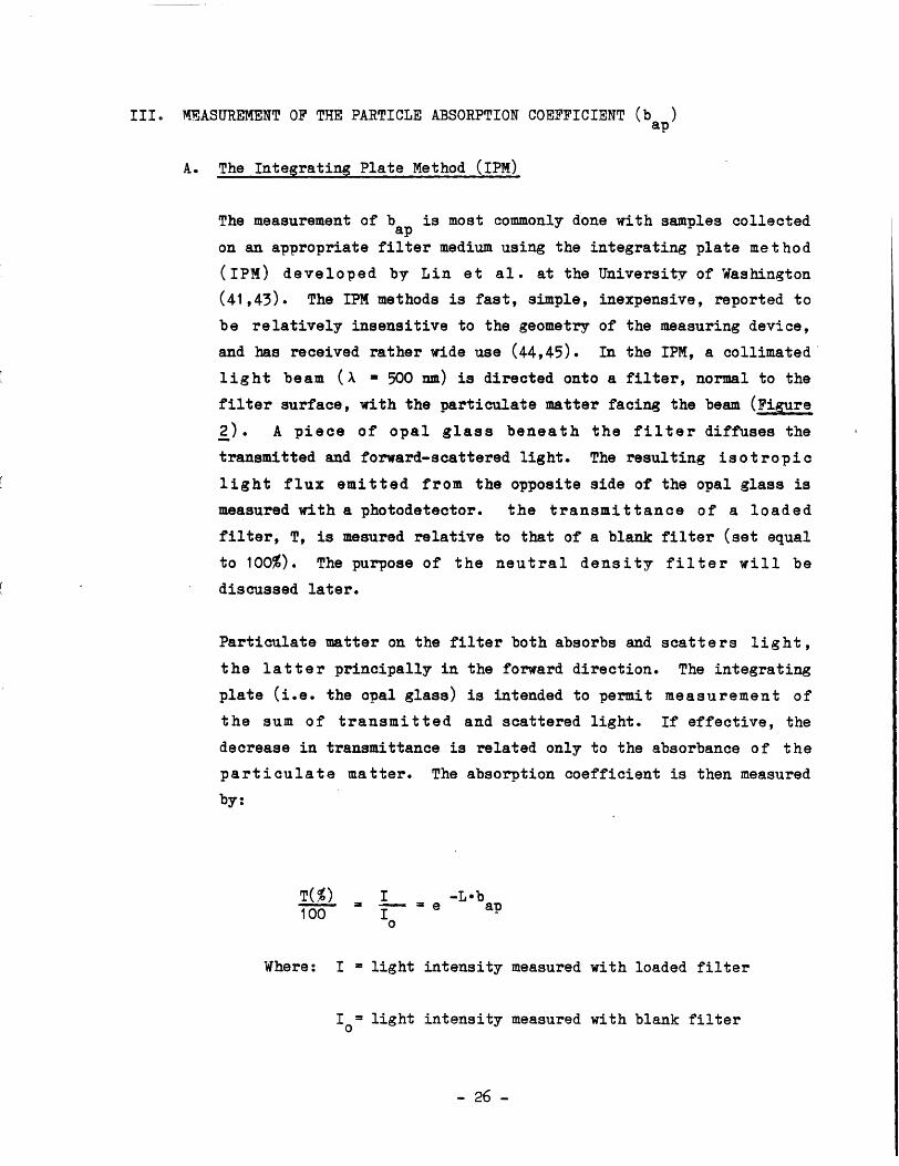
The measurement of b is most commonly done with samples collected ap on an appropriate filter medium using the integrating plate method

( IPM) developed by Lin et al. at the University of Washington

(41,43). The IPM methods is fast, simple, inexpensive, reported to

be relatively insensitive to the geometry of the measuring device,

and has received rather wide use (44,45). In the IPM, a collimated·

1 i g ht be am ( A • 500 nm) is directed onto a filter, normal to the

filter surface, with the particulate matter facing the beam (Figure

~). A piece of opal glass beneath the filter diffuses the

transmitted and forward-scattered light. The resulting isotropic

light flux emitted from the opposite side of' the opal glass is

measured with a photodetector. the transmittance of a loaded

filter, T, is mesured relative to that of a blank filter (set equal

to 100%). The purpose of the neutral density filter will be

discussed later.

Particulate matter on the filter both absorbs and scatters light,

the latter principally in the forward direction. The integrating

plate (i.e. the opal glass) is intended to permit measurement of

the sum of transmitted and scattered light. If effective, the

decrease in transmittance is related only to the absorbance of the

particulate matter. The abso?'J)tion coefficient is then measured

by:

T(%) I -L•b = - = e apToo I

0

Where: I= light intensity measured with loaded filter

I= light intensity measured with blank filter 0

- 26 -

INTEGRATING PLATEFILTER PARTICLE~ I

..ILLUMINATION ..LIGHT .. ►

NEUTRAL DENS ITV .FILTER / SCATTERED LIGHT

Figure 20 Schematic of Integrating Plate Method (IPM).

- 26a -

L ~ the ratio of the air volume sam~led to the

particulate deposit area on the filter

ln I /I0Thus: b ~ in the units (distance)-1

ap L To yield accurate absorption coefficients, it is necessary that the

r incident beam strikes each particle only once, and that light

absorbing particles not be shielded by other particles.

Accordingly, particle loadings< 20 µg/cm2 have been recommended.

Use of a filter with minimal absorbance also should increase the

precision of measuring b • The Lin procedure uses Nucleporeap filters, which provide low absorbance, a refractive index similar

to that of atmospheric -particles, and minimal penetration of

particles into the filter so that multiple absorption is minimized.

(_

The Lin -procedure is subject to error due to multiple reflection

between the up-per surface of the o-pal glass and the Nuclepore

filter. This multiple reflection provides an o~portunity for

multiple absorpt;i.on of light by the particulate matter. · To

minimize this effect, a neutral density (ND) optical filter was

inserted between the Nucle~ore filter and opal glass (43). The ND

filter attenuates the multiply-reflected light.

In support of this technique, Lin reported (41) that a 'Nuclepore

filter loade~ with non-absorbing NaCl aerosol exhibited a

transmittance of 99%, indicating that the light scattered from

these particles still reached the detector. Since no neutral

density filter was employed with this experiment, and the particles

faced away from the light source, this value may have limited

relevance to the IPM as currently done.

A more recent evaluation (45) with a non-absorbing aerosol

(NH4) 2S04, as well as mixtures of absorbing and non-absorbing

materials, also done without an ND filter, revealed a small

- 27 -

apparent absorption for (NH4) 2S04, about 1% of that for an equal

mass of carbon (soot).

For the present study our objectives we re ( 1 ) to eva 1 ua t e the

sensitivity of the technique to wavelength and geometry, (2) to

evaluate and im-prove, if necessary, the precision of the method,

(3) to evaluate factors influencing the accuracy of the method

(e.g. the use of neutral density filter), and (4) to compare

results with those obtained by University of Washington personnel

with the same samples. Appendix C details these evaluations.

The precision of the IPM method with loaded filters was found to be

0.3 to 1.4t coefficient of variation (c.v.). In parallel

atmospheric sampling, the c.v. between samplers was i 1.7'1,. A

comparison with the University of Washington yielded % transmittance (T) values for loaded Nuclepore filters which agreed

within 1 to 2% T.

The accuracy and precision of the method varied with loading. Very

lightly loaded samples gave reduced precision. However, sam-ples

with particle loadings > ca. 20 JJg/cm2 no longer approximate the

requirements for the IPM method. Accordingly, in the present

study, -parallel atmospheric samples were collected with 25 mm and

47 mm filters at the same flow rate (8 Lpm) to obtain particle

loadings per unit area differing by about a factor of five. It was

intended that at least one of the sample pairs would provide an

appropriate sample. In this sampling, the loadings on the 47 mm

filter samples were i 16 µg/cm2 , and, except at San Jose, most of

the 25 mm samples exceeded 20 µg/cm2 loadings.

Figure 3 compares b determinations for the 47 and 25 mm filter ap samples. Samples yielding b values < 0.04 have been excluded. ap The data show good correlation and a ratio of mean values, 47 mm:

2 5 mm filters, of 1.04. Nevertheless, the least squares slol)e and

intercept differ significantly from 1.0 and zero, respectively (p =

O. 99). We consider the b values< 0.1 to be more reliablyap

- 28 -

Figure 3. Comparison of b Measurements at Two Particle Loadingsap

1.6 0

0 1.4

-I 1. 2E ..... I

ts}__. 1.0

~

L QJ

I _µi r-t.,

•r-1 0. 8

/ /

/ /.,,,,,I 4- 0 ·/

E E 0. 6

0 0 . // / / /~ ~ / //..._, Y = -0.046 + 1.21X

/

/// .. ~ ~c;

/ / ~<:,UY

./ / 'i,~~t-,.'v

/

/ /

/ /

~ /

/ /

0. 4 8-_!)

(fj0. 2 0

0.0L,Q?00°0

0

0

0

/~

0. 0

·/00~ / .

~,,,,6 0 0 r - 0.956 0

1 I0. 2 I I I I I0. 4 0.6 0. 8 1. 0 1. 2 1. 4

bap (25 mm filter) 10--1m-1

measured by the 25 mm filter. Values > 0.6 are considered to be

more reliably measured with the 47 mm filter.

B. A Laser Transmission Method (LTM)

Rosen et al., at the I.a.wrence Berekely Laboratory, have devised a

version of the IPM which measured the transmission of 1 i g ht from a

He-Ne laser (632.a nm) passing through atmospheric particulate-loaded

filters (42). In this system the integrating plate is eliminated and

the filter, itself, is used to provide uniform intensity to all

forward-scattered light. In addition, a large lens immediately

behind the sample filter is used to focus the light onto the

detector, increasing the sensitivity of the measurement and possibly

decreasing errors due to light scattering. The decreased light

intensity reaching a detector relative to that with a blank filter,

is assumed to be due to light absorption by the particles.

The reported advantages of the LTM compared to the IPM, are its

applicability to more heavily loaded samples, and the suitability of

filter media other than Nuclepore, including quartz fiber. The

latter would also permit combustion analysis for total, organic and

elemental carbon. Accordingly, this technique was included in the

present study.

Figure 4 compares University of Washington IPM and LBL LTM results

for co-collected samples (46). The LTM method was used with both

Millipore cellulose ester membrane fil tars and prefired Pall flex

quartz fil tars. The LTM method showed reasonable agreement for the

two filter types but differed by, on average, a factor of 2. 5 from

the IPM. R. Weiss (47) believes that the factor of 2.5 higher

results by LTM is due to multiple absorption because particles

penetrate substantially beneath the cellulose ester and quartz filter

surfaces. Within the filter matrix, each particle could intercept

the incident light more than once as the light is scattered by

surfaces. Since the IPM has been reported to measure b with an ap

- 29 -

,{

f I,

----

X

X

.xf~

X

~ NUCLEPORE ·1. vs

__....,-I NUCLEPORE vsE ,o-4

MILLI PORE

__...., uJ a: 0 a.. IJJ 10-5

•_J ~ I u ::> z X ••x

x•

•

QUARTZ .._...,

C.

bo 10-6

:e: X 0--

Figure 4 Comparison of the Integrating Plate Method and Laser Transmission Techniques for AbsorptionCoefficient Measurement (x =Millipore,•= Quartz)

- 29a -

error of ~ 15%, (43) the b measurements by the LTM would requireap

substantial correction. However the LTM was also compared to a

photoacoustic method and showed almost perfect agreement (45). When

compared to a similar photoacoustic method, the IPM gave higher

results by a factor of 1.3. Given these inconsistencies, the factor

of two uncertainty ·in absorption coefficient measurements estima tad

elsewhere (45, page 28) seems prudent.

Figure 5 is a diagram of an LTM apparatus as constructed at AIHL.

The unit differs from the LBL apparatus principally in the detector,

a photodiode/op amp in place of a photomultiplier tube. Our initial

evaluation of this technique considered: (1) Linearity of the

detector response with change in light intensity, (2) precision, (3)

effect of filter medium, (4) effect of particulate orientation

( toward or away from the light source), (5) comparison with the IPM

for b measurement, (6) the influence of wavelength, and (7)ap

comparison of LTM results by AIHL and LBL.

As detailed in Appendix C, linearity was excellent throughout the

range relevant to loaded quartz filter samples. The precision of b ap

measurements was 2 and 4-4% (c.v.) for Millipore and quartz filters,

respectively. Analyses of the same filter samples by AIHL and LBL

showed high correlation (r = 0.9999).

c. Comparison of b Determinations by The IPM and LTM a

Figure 6 compares results by the two methods for the atmospheric

samples collected at the three sampling sites in the current field

study. For this comparison, IPM results with 25 mm and 47 mm

parallel fil tar samples were averaged, except where one or both b _ 4 _ l ap

values was < 0.04 X 10 m • For such low absorption coefficients,

the higher face velocity results (i.e., those for 25 mm filters) were

considered mo re accurate. The results are highly correlatad. The

ratio of mean values LTM:IPM is 2.72. Since the preponderance of

current data suggests the IPM to be more accurate for the measurement

- 30 -

f.Sample

D I D He-Ne Laser Lens

A Lens

B

Detector

Digital Voltmeter

~PVC Light-Tight Box Slide mechanism to insert and withdraw sample supported in rigid frame

Laser: 632.8nm, O.Smw, Spectraphysics Model 155, random polarizationG

Lens A: 12.4mm diameter, 14.3mm focal length, plane-convex lens to expand beam to a 1.2cm diameter disc on the filter sample.

Lens B: 60mm diameter, 39mm focal length, aspheric lens, Rolyn optics.

Detector: EG & G Model HUV-1 OOOB silicon photovoltaic detector/operational amplifier combination, positioned at focal point of lens B.

DVM: Fluke Model 8000A digital multimeter.

Base: 1/2" flat steel plate optical bench permitting use of clamps with magnetic bases.

Enclosure: 1/2" PVC sheet.

Figure5. Schematic Diagram of Laser Transmission Method, Viewed From Above.

(not to scale)

- 30a -

Figure 6. Comparison of b Measurements by the IPM and LTM Methods ap

- . .--------•••-'•·- csu,-•-·•-•-••~-~- • -

1~5

0

I um ... I s

1 ts;)

I ...... .75 t ..tr . I ,,...,.

X n.. '-' ~

.50t ...0

.25

BAPIPILTMSYNBOLa. LUETYPE11

~!t)c

a--5. 2116 •.al. 5138 bee•.«« -.-=S.0176 -,..-e. 4528 · r-=0.9Z17

0L· L.•---- =------L-.~---~-- L----..-~~.l--."·-·---•-......~ 0 .50 1.80 1,50 ~ ~50 aae J_ ~c-~.

b•(LTM) 10-• m-1

-•-~ ...:::::=:;;£.:..z;;;;:::__.. ~l l~P ........a.._. WI ~....._, L.l.....~ ..::..:::J,i,.a.::...-::::.....i.-- rm--

of b , the LTM was judged potentially suitable only for elemental ap

carbon measurement.

f

(

(

- 31 -

IV. DETERMINATION OF ELEMENTAL CARBON (C)e

A. Introduction

Elemental or black carbon is the major contributor to the particle

absorption coefficient, b However, discrimination between ap organic and elemental carbon (C ) is difficult. A selective

e combustion method (SCM) and a reflectance method (RM) were

previously used for this purpose (34). The former gave results

which were believed to be in error by ca. 20%. The RM yielded

results which, with 24-hr hi-vol filter samples, were too low by a

factor of two. While more accurate, the SCM is slow and relatively

difficult. Accordingly, an effort was made to improve the

calibration of the RM. In addition, the laser transmission method

(LTM) was calibrated for use in measuring C. e

As detailed in Appendix D, for the current study the LTM as well as

the RM were calibrated with butane flame-derived soot of known

particle size distribut1.on prior to collection. In addition,

calibration employed samples supplied by LBL including diesel soot,

atmospheric particulates and vehicle tunnel air particulate samples.

The LBL samples were analyzed for elemental carbon by a thermal

analysis technique correcting for decomposition (60). The RM

calibration appeared to be relatively insenai tive to the source of

the carbon standard whereas the LTM calibration showed great

variation.

B. The Ia.ser Transmission Method for C (42).e

LBL has used the LTM technique to measure black or elemental carbon.

c = [c ] + [c ]total black organic

Thus by measuring total C and black C, organic C can be obtained by

difference (correcting for carbonate C if necessary). If black

- 32 -

carbon is assumed to be proportional to the absorbance of a loaded

filter:

1 =- - [Attn]

K

Where: Attn=- Attenuation=- -100 ln (I/I) 0

K =- a constant

The attenuation per unit mass of Ctotal' or specific

attenuation, a, is defined by:

K[cblack]

[ctotal]

Employing laboratory-generated and ambient air elemental carbon

samples, the LBL group determined a mean value for K of 20 2 .

cm /µg when deposited on a Millipore filter. Thus:

Attn=--20

c. Intermethod and Interlaboratory Comparisons

Calibrations results are summarized in Table 5. For ~ase in

iden tif'ica tion, the calibrations were coded as shown. Elemental

carbon values obtained with these calibration for ten fine

particulate atmospheric samples are compared to the corresponding

total carbon values in Table 6. Samples identified with the letters

J - Q were collected in Riverside and the remaining, in downtown Los

Angeles.

Comparing ratios of mean values, elemental carbon calculated from

LTM-1 (i.e. the LTM using the aged butane flame carbon) yielded

- 33 -

~

TABLE 5

CALIBRATIONS OF OPl'ICAL METHODS FOR ELEMENTAL CARBON

Code for Code for Carbon Reflectance for RM Laser Transmissionb LTM Source Method (RM)a Calibration Method (LTM) Calibration

Butane :Flame a= 0.0309, b = 1.68 a = 5. 59, b = 6 • 88 LTM-1 ( r = 0. 957) (r = O. 992)

LBL Carbon Samples a= 0.0366, b = 1.62 a= 11.1, b = 23.1 LTM-2 ( r = 0. 99) (r = 0.964)

LBL Samples and a= 0.0337, b = 1.65 RM-4 w Butane Flame (r = 0. 974 l,J

PJ

a. Slope, inte2ept and.correlation coefficient for the equation logy= log a+ blog x, where: y = (100-R) /200R and x = elemental or black carbon, µg/cm2 • R =%Reflectance.

b. Slope, intercept and correlation coefficient for the equation -100 ln (I/I)= a+ b (c ), where I and I are light intensity though loaded and clean filters, respect~vely, and C eis elemental or b~ack carbon, µg/cm2. 8

TABLE 6

COMPARISON OF TOTAL CARBON AND ELEMENTAL CARBON (C)e

VALUES (µg/m3) a

(

f

Sample ID

J11 59Q 11

M1176Q011

01183Q011

01185Q011

P1186Q011

Q1192Q011

T1202Q011

U1209Q011

W1214Q011

X1221Q011

Total C

25.15

18.03

13.89

12.0

16. 50

13.ao

17.02

4.46

36.16

13. 54

C e (LTM-1)

28.55

6.62

12. 37

11 • 51

22.88

9.24

25-6

7. rs,

59.34

10.03

C (LTM-2)e

5.gr

1 • 61

2.73

2. 56

4.,76

2.12

5.30

1.79

11 .83

3.99

C (RM-4)e

5.41

1.40

2.44

2.. 12

4.35

1.83

3.98

1. 01

11.00

3. 01

bMean C

e

5-64 ± .33

1. 51 ± • 15

2. 59 ± • 21

2.34 ± • 31

4. 56 ± .29

1.~ ± • 21

4.64 ± • 93

1. 40 ± • 55

11 • 42 ± .59

3. 50. ± .69

Ratio of Means : 1. 00 1. 13 0.25 o. 21 0.23

a.

b.

The terms LTM-1 , LTM-2 and RM-4 are defined

Mean of resul ta by LTM-2 and RM-4 methods.

in Table 5.

- 33b -

values which averaged 13% higher than the total carbon. Thus this

calibration was rejected as inappropriate. The remaining techniques

yielded C values averaging 21 to 25% of the total C. This compares e

to an average of 20% reported elsewhere by similar optical

techniques (59). The results by the laser method (LTM-2) were

higher by, on average, 19%, compared to those by reflectance.

Figure 7 is a scatter diagram of Ce determinations by LTM-2 against

those by RM-4 for about 100 fine particulate samples from the

current program. Symbols A,B,C,D indicate 1,2,3,4 data points,

respectively, at the same locations. The results are highly

correlated, show a negligible intercept, and average 15.5% higher by

the LTM.

Eight respirable particle samples which, by our optical methods,

ranged in C loading from 1 to 8 µg/ cm 2 , were analyzed by the e

General Motors Research Laboratory. In the GM technique (49) filter

samples are dropped into a furnace at 950• in helium. The evolved

pyrolysis products are subsequently converted to CO 2 and analyzed by

a non-dispersive infra-red method to yield "apparent organic

carbon". Oxygen is then introduced into the furnace section

containing the sample and the resulting CO 2 is used to measure

"apparent elemental carbon". The method is believed to be subject

to error from charring during analysis which would yield elevated CE

values.

Table 7 lists the AIHL and GM results. The AIHL values show

C obtained by the LTM, RM and mean values by those techniques. In e

addition to C results, GM's values for organic carbon are also e

given. The optical methods were highly correlated with the GM

values (r ~ 0.95) but yielded results which were about 25% lower.

Given the uncertainty in defining organic and elemental carbon in

atmospheric samples, none of these methods can as yet be considered

to be more nearly "correct".

-----------

---------

Figure 7. Elemental Carbon by the LTM vs. Reflectance Method

/ A11 +

__ / A

10 + /

-/ A

/9 +

/ I

- I - -- ------- ---- - -- - ---- ---- ----- ------ --/a +

I --- - --- - ------ ---------'--------- - --- - -- -- ---- -I - - ---· ~~,L_

7 + ~ -- - -- - -a->'#'~ ----- --- . RM-4 / _,,.i,~7-- -- -- ----

C (µg/m1e

6 +

I w I•-... IU 5 +

---------------

__

-- / _-

/A-- --✓- --- A

- L ------- / - B

/_A------7 ·-= A

_____ _x_ = r =

-0.075 + p~~'!~~­'--------4 + 0.986

- 3 + __ _

I' - -- - -2... - --

1 I -~AA:1 + ~E'3~

I("_· BA

~

_Q_ ~ -+---------+---------+---------+---------+---------+---------+---------+---------+---------+---------+---------+---------+--· o 1 2 3 4 5 6 7 e 9 10 11 12

LTM-2 C (µg/m 3)e

TABLE 7

COMPARISON OF ELEMENTAL CARBON MEASUREMENTS BY GENERAL MOTORS' COMBUSTION AND A.DIL OPrICAL METHODS (l,lg/m2 )

C C e 0

Sample LTMa RMb

J1161Q011 2. 92 2.49

L1169Q011 1. 07 0.94

R1194Q011 2.67 1.95

R1196Q011 1. 20 0.82

V1210Q011 s.35 6.55

W1217Q011 3.32 2 .. 63

X1218Q011 8.01 7 .16

X121 9Q011 5.05 3.96

Blank 0 0

Regression F4uations: Mean C =- -0.141 e

LM C == -0 .. 36 e

RM C = -0.375 e

a. Laser transmission method. b. Reflectance method. c. Mean results by the LTM and RM.

C cMean e

2 .. 70 ± o.o;

1. 01 ± 0.09

2 .. 31 ± o. 51

1. 01 ± 0.27

7. 45 ± 1. 27

2.gr ± 0.49

7. 59 ± o. 60

4. 51 ± 0.77

0

+ 0.748 (GM C)e

+ 0. 845 (GM C )e

+ 0.702 (GM C)e

GM

;. 9 ± 0

2.4 ± 0.1

3. 5 ± o. 1

2.3 ± 0.3

11. 0 ± 0.4

;.2 ± 0.1

8. 6 ± 0.1

7 .1 ± o. 3

< 0.1

r = 0. 956

r=0.969

r = 0. 947

GM

12.4 ± 0.4

9.1 ± 0.3

9. 5 ± 0.5

7.6 ± 0.4

18. 1 ± 0.8

8.7 ± 0.4

15. 2 ± 0.8

11.s ± 1 • 5

1.8 ± o.a

- 34b -

D. Comparison of C by Optical Methods with Particle Absorptione

Coefficient Results

Since C is the nearly exclusive source of light absorption in e

suspended atmospheric particles, and since most of the C is in the e

fine particle fraction, a linear correlation is expected between

fine particle concentration C and the light absorption coefficient a

(b ) • For example, Figure 8 shows General Motors' results for ap Winter Denver aerosol (6). The mean slope was 11.8 m2/g (0.118

_4 x:10 m2/µg) and correlation coefficient, 0.93. The bap values for

{ the Denver study were obtained by the integrating plate method

( IPM), (but without a neutral density fil tar as employed in the ... present study) and Ce, by General Motors' controlled combustion

technique ( 49). The latter yielded results equal, within

( experimental variability, to the interlaboratory mean values for C a

and organic carbon C by combustion methods with 24-hr hi-vol 0

samples, in the GM Round Robin comparison.

( Figures 9 - 11 are scatter diagrams for about 100 atmospheric

samples from the present study plotting, C (LTM-2), C (RM-4) and a a

mean fine particle C a

values against means b ap values by the IPM.

The intercepts are negligible in all cases, and the mean slopes are

( 11 • 1 , 12. 9 and 12. 0 m2/ g, res pa c ti v e 1 y • Thus the r a s u 1 t s a r a

similar to those by GM in Denver, implying reasonable agreement

between our optical methods and GM's selective combustion technique.

These values for atmospheric C may be compared to the absorption( e

coefficient per unit mass ·for soot. Heitzenberg reports a value of

*Better accuracy is expected for the IPM with N.D. filter. The GM b values( ap

are inferred to be 5-10% too high (50).

- 35 -

0

I -....

•J II.

•-.. 0.• -Iii

.,e o c.S

·-l ..,o.. •-C!-

•1ft d

I

••

•

• X

• •

•

11 11 a ,p 1D •PLne EL...,,iaL Carbon 1J9I•

Figure 8. Relation between Absorption Coefficient and C for eDenver Winter Aerosol (Ref. 6)

- 35a -

----- -- --------

---

Figure 99 Elemental Carbon -by LTM vs. Absorption Coefficients

___ 1 .. 4 _+ _______ ------ --- ----------- ---------- ---------- -----------~·- ------ - --------•-·--··--·--A

1. 3 + . _ ------- ----------------

_ 1. 2 -t- -- --- - --· -1

A .l.l_-1-__________________________

I I

_l. Q __-t____ ---------------- ·------- -- ------------------

-- 0. 9 --+

I bap _Q.8_:t- ________________ ----------- ------- - -------·- -------------- ----- ____________________,__________________

---------------------

----------

4 1 (10 m-) 0.7 - -------------------------- _____,., ---- --- -

------- -------~AA _A_________ ------

A A

. A - . A ____ A_B ___A_____________ ------

A A

A

__ o. 6 + ________________ _

_ O•. !:L-t-_ _____________ y = -0 o 053_7 +__ 0 o lllx_ r = 0.925

__ 0.4_t___ ------------------------A

_o. 3_+ A

A ~ACC0.2 + _ AACC AA

BBB A A BA A A _.7n AB

0. 1 + B ,,A'd'AA - A . . . I A A 1AA A AAA l A~.(c AA

0 .. 0 -+~~-~-B_~__ A_ __ ----~---------_ -----~ ______________ - +-- _______________ +-------_-- ______ ~- _-------- -----:;_-------·-;-···- -------------:;:- _____________ ~- _________ -+- _____ ... __ +. I w U'l o 1 2 3 4 s 6 7 a 9 10 11 12 t:1

LTM-2 C . (µg/m 3 )e

- ------- - ------ ---

,=

b ap

_4 _l (10 m )

w

_,........,_ ,,-,, ,....,,""" r"- - ..."..

Figure 10 Elemental Carbon by the RM vs. Absorption Coefficients

1. 4 + : A I

-1 ~::i-- ± ---- ------------------------ --------

--1. 2 + --------

1.1- +_ ____________________ AI ----·---- -- -- -- - ----------

LO+

0.9 +

o.a + I. I

__ Q. 7. -t. -- - ------·--. ----- ----------~-------------- -

I A

--v. 6- ---------------- -----;JC- ----------- ·----- - . - ---··· -- -- ---- ------

1 _Q_!L~ --------·--------- .. -Y =-o .037__ ,t __Q!..~ ~~-­

A ,;/'A A A r = 0.917

C. 4 +__ -- -·--·------------A ----- -------A ;/-A,______ A _____________ ---

A _Q •. 3 ± ___ ------ __________A___L__A__ ----

1 BA~ A A A AA1,,AAAB AA

0. 2 + --------- --------- ------~ACD____A_______________ ------~- _____________

AC~ A BA A A

0. l + AAy("B :·A____ A

I ~BA BAA

a. a !L~~;::..~ _ .. ---+-- _ -+ _ _ _ _ ·+ _ ___ :. _ _ :.:. _ __ + _ _ -+-- .. . __ + --------+ ____ 0 lJl

0 1 2 3 4 5 6 7 8 9 10 11

RM-4 C (µg/m 3) e

Figure 11. Mean Elemental Carbon by LTM and RM vs. Absorption Coefficients

1. 4 + --- ---------- --·-------~------- --·----- -----A

..L--1,_±.__________

L-2-~----

A -1~1-±-

1 I

-1. 0 -t.______ -- ----- --- ---------

: a

0_9_

b .0.8 + --------- ·-------- - ---- ---- ---ap

_4 -1 : ( 10 m ) Q_7 .+____ A

0. 6 +__ -----

_Q_ 5 + -- --- -- -- .. ---------------- - --------· AA A--1('~-------- ----------

y =-0.0483 + 0.120x0. 4 +. .. - - --- A - ·-- - -- ··- -· . A -·-------- --\0" r = 0.924

/2 A A _Q.3 + ----- - ----·-------- ----

B A ~

A A C.,,J:_A A A A 0.2 + . --~---EC __ .A.- ---------·- -·-· .. ----------------------

,,,,KAA B AA A Atl.A A0. 1+ pJB~A A.

I A Bt A BA I _),AB AA

w 0.0 ++~-~AAA:--~-----+--------+---------+----- __ -~-- ------+-~ ----+--- -----♦---------♦ ---------+---------+-----U1 p., 0 1 2 3 4 5 b 7 8 9 10

Mean C (µg/m 3)e

11

These values for atmospheric C may be compared to the absorptione

coefficient per unit mass for soot. Heitzenberg reports a value of

9.7 m2 /g ( 13) but notes that in mixtures with non-absorbing

material, the value increases. Clarke and Waggoner ( 50) report a

mean value of 10. 1 ± 2 .1 m2 /g ( n = 4) for soot collected on

Nuclepore filters.

Previous studies showed measurable absorption by coarse as well as

fine particle C. Employing mean C values and multiple regression·· e _ e analysis for 104, four-hour periods yields the equation (in units

- L+ 110 m- ):

b - - 0.04a ± 0.15 + 0.116 ± o.ooa (c )f. + o. 02 ± 0.029 (c)ap e ine e coarse r • 0.925.

Thus the absorption efficiency for coarse C , per unit mass e

concentrations, is not significantly different from zero.

Furthermore, the addition of coarse C does not significantlye

improve the correlation with b (r = 0.924, Figure 11). Hqwever,ap

as will be shown in Section VIII A, fine and coarse elemental carbon

show a relatively strong linear correlation ( r = 0.81). As a

result, the standard deviations for the coefficients in the multiple

regression with b are increased. Thus coarse elemental carbon mayap

have a relatively small but real contribution to light absorption.

- 36 -

V. MEASUREMENT OF THE SCATTERING COEFFICIENT FOR LIQUID WATER

A. Introduction

Water is a significant constituent of suspended particulate matter

and contributes to light extinction by light scattering. To

estimate the contribution of such scattering, two integrating

nephelometers were operated side-by-side (Appendix B) with the

incoming sample of one unit heated 16 + 3° C above ambient,

following the recommendation of A. Waggoner, to dehydrate the

aero so 1 • The s cat t e ring co e ff i c i en t f o r watar, b , can beSW

calculated as the difference (b ) bi t- (b )h t d. In spam en sp ea e principle, this technique is subject to error since other aerosol

constituents, including organic compounds, NH4No 3 and halide salts,

might vo lat i 1 i z e as we 11. However, it should provide an upper

limit for the scattering coefficient for particle-bound water.

B. Method Evaluation and Correlation with Aerosol Constitutents

The water content of atmospheric aerosols should vacy with relative

humidity as well as the aerosol composition, since both sulfate and

nitrate aerosols are hygroscopic. Table 8 lists Pearson

correlation coefficients between b , pollutant and meteorologicalSW

parameters as well as visibility parameters as measured in the

current study. The highest correlations (0.6 - 0.7) were found

between b , fine sulfate, ammonium, fine mass, and b , the SW ag

absorption coefficient f_or NO 2 • If volatilization of organic

compounds was an important contributor to b , as measured by the SW

difference method, then a higher correlation between b and C SW 0

would be expected compared to the 0.32 observed.

To assess the combined influence of RH and aerosol constitutents

b data were fit to equations of the form: SW

- 37 -

Table 8

PEARSON CORRELATION COEFFICIENTS BETWEEN b ,SW

POLLUTANT AND METEOROLOGICAL PARAME'rERSa

Parameterb r

= FS04 0.74

= CS04 o. 54

,f

FN03 - 0.48

CN03 - 0.4;

HN03 0.. 29

NH4 + 0.. 7;

0.05CNH3

FC 0.27 e

cc o. ;1e

C 0.. 32 0

F Mass 0.64

03 0.19

RH 0.41

T - 0.06

b 0.67 ag

b o. 58 sp

b o.. 18 ap

a .. b .. c.

n = 107 - 109 F = fine , C = coarse Not significantly different from zero

- 37a -

b SW

= a + + ( 1 )

and

(2)

Where x and y are constants between 0 and 2, andµ=% RH/100.

The results shown in Table 9 indicate a general improvement in

correlation relative to linear regression with two parameters.

However employing equation 1, the addition of a relative humidity

factor shows only a small improvement in the correlation with

little change for x • 0.5 to 1 .o. Similarly, using the other

equations shown in table 9, there is relatively little change for x 2

or y =- 0.67 to 2.0. The range in the variance, r, with equations

including humidity dependence was only 0.6; to 0.66. Based on the 2

criterion of maximizing r, clearly the choice of a specific model

from the six listed is not crucial. For simplicity we have

employed equation 9-2 with y =- 1.0, although most recent studies

have used equation (1).

2 2 The correlation obtained here (r =- 0.66) compares to a value r =

2o.a7 observed in Denver with equation 9-1, x = 1 and r = 0.17 with

the same equation in the eastern U.S. (51). Poor correlation was

suggested to be due to the lack of speciation of sulfates since

H2so 4, for example, is more hygroscopic than (NH 4) 2 S0 4•

- 38 -

Table 9

MULTIPLE REGRESSION ANALYSIS BETW~EN b AND AEROSOL CONSTITUENTSSW

E9.uationa

X _J_ a b b C r r2

9-1 o.o - 0.029 0.046 00023 0.76 0.58 0.5 - 0.039 0.031 0.019 0.79 0.63 0.7 - 0.034 0.026 00018 0.80 0.64 1.0 - 0.015 0.019 0.015 0.81 0.65

9-2 0.67 - 0.031 0.069 0.047 0.81 0.66 1.0 - 0.012 0.081 0.062 0.81 0.66 2.0 0.083 0.125 0.115 0.78 0.61

9-3 0.5 - 0.039 0.044 0.040 0.78 0.60 1.0 - 0.03a 0.042 0.063 0.79 0.62 2.0 - 0.011 0.040 0 .. 125 0.79 0.63

9-4 0.5 - 0.039 0.044 0.019 0.77 0.,60 1.0 - 0.04 0.042 0.015 0.78 0.61 2.0 - 0.017 0.040 0.0073 0.79 0.62

9-5 0.5 - 0.0;4 0.066 0.024 0.79 0.62 1.o - 0.030 0.090 0.026 0.80 0.65 2.0 - 0.010 0.152 0.029 0.81 0.66

9-6 0.5 - 0.037 0.033 0.024 -0.79 0.62 1.o - 0.032 0.021 0.026 0.80 0.64 2.0 0.0037 0.0076 0.031 0.79 0.62

+ c(N03)aEquation 9- 1 : b = a + b~S0 4 ' SW

(1 - µ)x ( 1 - µ) X

Equation 9- 2: b =a+ b (S0 4 ) µY + c (NO 3) µYSW

Equation 9-3: b =a+ b (S04) + c (N03)µYSW

a + b (S04) + c (N03)::::zEquation 9- 4: b

SW ( 1 µ)x

a + b (S0 4 ) µY + c (NO 3)Equation 9- 5: b = SW

a + bS0 4Equation 9- 6: b = + c (N03)SW

(1 - µ)x

bNone are significantly different from zero at~= 0.95e

- 38a -

VI. ASSESSMENT OF SAMPLING ARTIFACTS

A. Artifact Particulate Sulfate on Glass Fiber Filters

Glass fiber bi-vol filters (Schleicher and Schuell, 1981 EPA Grade.

fired at 450°C) were used to collect samples for analysis of

carbonaceous materials. However, these were also analyzed for

sulfate and nitrate to assess what difference in sampling artifacts

resulted from the firing at 450°C relative to the filters as

received. In addition, glass fiber filters were assessed for HN0 3

retention with varying doses.

Figure 12 is a scatter diagram of blank-corrected sulfate results on

4-hour hi-vol glass fiber filter samples against those on Teflon

filters obtained in an open face 47 mm filter holder (i.e., without

deliberate particle size segregation). Riverside and Los Angeles

data were fit with a single line, and the San Jose data, with a

second line of markedly higher slope. Results on glass fiber are

significantly higher. The average difference (glass fiber)­f

(Teflon), was 4.9 µg/m3 • Thus, although the sulfate artifact is

smaller than expected for short terms samples (52) the positive

artifact clearly persists.

Bo Artifact Particulate Nitrate on Glass Fiber Filters

Previous studies with 4-hour hi-vol sampling have indicated that at

least for short term sampling, glass fiber filters serve as total

inorganic nitrate (TIN) collectors, retaining both particulate and

gaseous nitric acid (21). The present study repeated this

comparison at San Jose, Riverside and Los Angeles and, in addition,

evaluated 16 to 24-hour bi-vol filters (prefired S & S glass fiber

filters) as TIN collectors. For this purpose, N0 3- on glass fiber

filters was compared to the sum of the nitrate retained by Teflon

filter and a NaCl-impregnated filter sampling in tandem.

- 39 -

Figure 12. Artifact Sulfate ·on Glass fiber Filters, 4 Hr. Hi-Vol

r·· ---- -----,,.,/

40~. / /_," ✓i + SAN JOSE

0. .,/

/

/

l O RIVERSIDE / /,.

,.., ✓

35~ l

o LOS f.NGELES / ," i

(fl .,/' / E ! _.,/ /

'­~ ,/ ,.._ ,

// ~...,.,,m 30 i-' :) //o ,..~v./

" ~"Y.,◊ / .ci..V'

,,........ ◊

;~--✓ -

0 ~-0~) /'

0 0:: 2s l-UJ 1 ~6 0 ~g,,

cP / /'m I _,'6w 1---j I 0/ /~ LL ., /

20 L. ,p·/ /.,.0 U)

¢◊◊ /. 0 ./(f) <t:: !

_J I $ ~~~ / ◊ /9'bo /~ 15~

'-"" 0~~800 /o·~C tf ,/

+ ~~i /10 I - ✓~-. 0 ◊ /0""""' (f) ! ,~-- /

l_,,~"" /', i· .,r +./~ ,5 t-;;t_.,, /

: ~ /

i *+ ~;1:i ~

✓

0 L --- -- .. j__________J___ ·- _--.....L .. -- .. ____L . ··---·--- .L ~,. _. -1... --- ·-· -- 1.______L 0 5 10 15 20 25 30 35 40

so_.2- (TEFLON) ug/m3

Samples

SAN JOSE SYMBOL=+ LINETYPE= · · · · · · · · · · · · y=a+b*xt1=36 a=l.9337 e

11;:0. 9219

b=l. 7590 s 11=0. 3902 s.,..=1. 6798 r=0. 6116

RIVERSIDE &LOS ANGELES SYMBOL=o LINETYPE= -----------y=a+b*xn~7~ a=6.5235 s.=3. 4016 b=0.9326 s.,=0. 0297 e-,.x=l. 6570 r=0.9673

Figure 13 compares 4-hour results for the three sites. The results

are highly correlated, with a ratio of means (glass fiber N0 3-)/TIN

of O. 997. Thus these data also support glass fiber filters as TIN

samplers.

The 16 to 24-hour hi-vol filter nitrate data are compared to the

corresponding TIN values calculated from 4-hour samples in Figures

14-16. Only at San Jose, which exhibited low nitrate levels (TIN i 32 1,1g/cm2) did the glass fiber fil tars continue to approximate TIN

samplers (ratio of mean, glass fiber/TIN• 1.03). At Riverside and

Los Angeles, an average of 24 to 42% of the nitrate (presumably

HN03) penetrated the filters. The difference in results with

location probably results from the much higher nitrate dose in the

Los Angeles basin(~ 147 µg/cm2 TIN).

c. Loss of Particles in the Denuder of the Particulate Nitrate (PM)

Sampler

Previous studies have suggested that coarse particle nitrate may be

1 ost in transit through the diffusion denuder employed to remove

HN03 from particulate nitrate leading to negative errors in

measuring PN. To minimize such errors the present study measured

fine particle nitrate, excluding coarse nitrate and other aerosols

from the denuder with a cyclone. Loss of < 2. 5 µm nitrate was not

expected to be significant. However, if it occurred, it would

produce a· negative error in the fine particulate nitrate

measurements.

To measure the loss of fine particle constituents in the denuder, it

is necessary to compare concentrations of a stable species collected

on a filter with and without a preceding denuder. Sulfate collected

on Teflon filters was used for this purpose. Figure 17 compares

results for sampler 3 (with denuder) to those for sampler 1 (no

denuder), and indicates very high correlation of results and no

significant loss of sulfate in the denuder. Although sulfate

- 40 -

r~

E " "'-m J

'-"

Cl)

0 z a:::I~w

PJ Q.

CD .,.._..I

LL

(J) (J)

< _J ~

FIGURE13 Nitric Acid Retention on Glass Fiber Hi-Vol Filters, (4 Hr.

60 r------ss r / 0

s+ V' / 0

+ s. J.. (),

◊ RV45~ 0 LA. i ) ,0. / 0

40l -✓I .A_ 0

35

030

2l I

""-.20

15' l

r-ml

I

r-

slit◊ LJ0L...- I I I I 1----L-___ L.___ I -- l l l __ L__ 0 5 10 15 20 25 30 35 40 45 50 55 60 65 70

TOTAL N03 (u9/m3)

Samples)

NITRATE SYMBOL=·LlNETYPEr: y=a+b*xn=104 a=t.3808 e.=0. 5152 b=0.9349 sa.=0. 0190 s,_,.=3. 0401 r=0.9796

,t

l

r- Y = 1.23 + 0.855 X

~ r = 0.939

+I-

..

-~

~

1. +

...

...

+

Figure 14. Nitric Acid Retention on Glass Fiber Hi-Vol Filters (San Jose, 16-24 hr Samples}

~

!llr-.. I

10 1

I

~ e 9!-

I

i' tn ..._,:)

8 i-I I

C "" I

z 7~ l

0:: w co 6~ t--t I LL

5~(..f) I (Jj

< --1 4l..... L? l

l I~--L..

~ (\J

I 2~cc __.

lr I

I...0L_ I

0 1

i 1 I

!

I I I I ....L.. t I I I -L..-t~...-1.......1-._.L__.J__ 1 g2 3 4 5 6 7 8 10 11

16-24 HR MEAN TOTr,L N03 (ug/m3)

- 40b -

I

12

t:;' E

' O') :) ~

{

0 "' z a:= LU CD ....... LL.

CJ1 en < _J 0

0::: ::r:: ..:t N I

(0 ......

Figure 15. Nitric Acid Retention on Glass Fiber Hi-Vol Filters (Riverside, 16-24 hr Samples)

30 I -----·-------·-•-····-·--··-··---·--1

I

29·I ' I r ir ;

' 281r i

27·t

r 25~

I

i 25~

;

l 24t-

I i

2sL l t ' 22L. I

2'i ' I

j I I

·r I I20L.. ! I

!1aL j

Y = 3.47 + 0.646 X r = 0.881

!

I ! \

! i

18 ~- .L ___ ____J_J t! ..L.,.___.,__,_.____ .J~-L I 1-.L-l----.il..--._l L._J___J__ J I

20 21 22 23 24 2s 2s 21 2a 29 a0 s1 32 33 34 ss 36 37 38

16-24 HR MEAN TOTAL N0 3 (u9/m~

- 40c -

~ E

' en ::)

'-'

('l't

0 z ~ w CD ........ LL (/) (/) <C: __,' t:)

er: :r: ~ ('\J

I co .-t

Figure 16. Nitric Acid Retention on Glass Fiber Hi-Vol Filters (Los Angeles, 16-24 hr Samples)

I 30 ·---, ~

fI Ii·"9

i t Y = 9.87 + 0.27 X ~ l i· I r = 0.909 t-

ii l

! I""

ol 25L

i

.. ~

I i

l

' l r • I r I I

020 r-1 o. I

r I

0 I

i..

L I I

i i +-l

15 r-1 I

0l I 1. I I 1 LJ.....1.-l- I I I I I I I LJ-a I i I -.. I I I I 20 25 30 35 ' J 40 45 ' 50 55

16-24 HR MEAN TOTAL N03 (ug/m3)

- 40d -

~

Figure 17. Loss of Non-Volatile Particles in the Denuder for Nitrate Sampling

(W)

E

' m J

~ I (Y)

i> ~

n:: I LL.I

___j

(L ::E < (f) '-../

...,. 0 (ID

40 ~ ·--··-· ~

3BL L

361-.....

34 ,-. ~

32~ t

30r +-

28 L 26;_

24l ;

22~ I

1-

20 ~ r

18 r-....

16~

14~ +-

12 f­~

10~ l-

8 ~ r--

6 ~ ,- i-

4 ;_

+ s. J. ◊ RV o L.A.

0

0

0

,-..

! j

0 ~:.LL_LLLL LLJiLI.J..J ...LLJ.-1...L1._l_.1....L.J. l l I 1-1. J.i.J_Lt __ l._LLJ 0 2 4 6 8 10 12 14 16 18 20 22 24 26 28 30 32 34 36 38 40

S04 (SAMPLER 01) ug/m3

SULFATE SYMBOL==· LINETYPE== -­y==a+b*xn=108 a=-0.2214 s.==0. 1302 b==0.9910 s1.::;•t 0139 s,..•==0. 9030 r==0.9897

particles are expected to be somewhat smaller than nitrate (9) and,

therefore, not the ideal surrogate to estimate N0 3- loss, these

results do not support a significant error in particulate nitrate

measurement due to particle loss.

D. Loss of Non-Volatile Carbon in the Denuder of the Particulate Carbon

Sampler

To assess the extent of loss of non-volatile particles in the Al 2o3-

coated denuder of the true particulate carbon sampler, the quartz

fiber fil tars from samplers 4 and 5 were analyzed and comp a red for

elemental carbon by the reflectance method (RM-4), discussed

previously. Figure 18 is a scatter diagram of the Ce results, on

the two samplers. On average the loss of C was negligible.8

E. Retention of Carbonaceous Material on Hi-Vol Filter Samples

The retention of carbonaceous material on filters is the net result

of adsorption of gaseous organic compounds on filters a-nd on

previously collected particles, and volatilization from the filter

of initially particle-phase materials. Some insight into the

relative significance of such errors is obtained by comparing

results for a single long-term filter sample with a series of short­

term samples. Figure 19 compares observed total carbon values for

samples collected for 16 hours against 16-hour average values

calculated from four, successive 4-hour samples. Calculated values

are consistently higher, suggesting that adsorption of gaseous

species on relatively fresh filter surfaces and/or volatilization

from filters during prolonged sampling were important. Adsorption

of gaseous material on previously collected particles, which would

yield 16-hour sample results higher than those calculated from the

short-term samples, appears to be less significant.

- 41 -

Figure 18. Loss of Non-Volatile Particles in the Denuder of the Particulate Carbon Sampler.

1:t CW')-s ....... = .5

LO a: w ,_J a.({ :E <( rJ) m

CJ

t

8.00 ---------------------------

7.00

6.00

5.00

4.00

3.00

2.00

1.00

y = 0.0874 + 0.999x

r = 0.9985

0.00-------...._i.....i,_.._______......._.__.,__.__...___...__..____._-'-_._...._.,__,,--i.,__.__..._..i....., 0.00 1.00 2.00 3.00 4.00 5.00 6.00 7.00 8.00

C8 SAMPLER 4 (µg/m3)

- 41a -

>-0 => t-

0 ~ (J)

..Q,._, ta

>-c...>

r-1 t-ta +J 0 E-t 1--t ,._, ::, _j 0 :I: I t-i

\.0 CDr-1

"O Q) t--1 +J ta (J)

r-1 ::, CJ t--t

r-1 a > Cl]

::>

"O CD

Q)

::> a:::,._,

<QJ U]

..Q0

i-1°' N a, ,._, CD ::, O'I 0)

·r-1 ~ ~

·-\

\ -, •\ \

·.\

\ \

+◊o

un N

0 N

+

tl1 ,-◄

+ M,;:JO r-1 \.0 \.0 O"I

00

II II

~ ,._,

0 r-1

; i l

..... 0 LN

Il i ~

in

,......., ('Y')

~ O'I ;1....._,,,

a tJ.J >a:: w (I) CD a

<EUI/.6rt) 1J t3noH gt 031 v1nJ1VJ

VII. ATMOSPHERIC RESULTS, PART-- I

A. Tabulation of Results

Aerosol collection was done for 109, 4-hour periods. Table 10

compiles results for the more significant parameters measured

directly or indirectly for aerosol and gaseous pollutants. Except

as noted all chemical s-pecies are listed in µg/m 3 • Table 11

explains the meaning of the headings used. Table 12 provides mean

concentrations for the chemical sp~cies and meterological

parameters. The downtown Los Angeles site shows highest average

levels for sulfate and carbonaceous material. Riverside exhibited

the highest particulate nitrate.

B. Summary of Visibility Results

Table 13 lists mean and maximum values measured for visibility

parameters at the three sampling sites. Mean values are for 30 to

36, 4-hour periods at each site.

Light scattering by dry paticles (i.e., b as measured by an . sp integrating ne~helometer heated 16 ~ 3°C above ambient temperature)

was the largest contributor to the total extinction at all sites,

representing somewhat more than half of the extinction coefficient,

b'ext· Light absorption by particles, which can be related ~lmost

exclusively to elemental carbon (42), was relatively small at sites

in the Los Angeles basin where high concentrations of efficient

light sea tt e ring species were present. However, at San Jose

absor~tion averaged nearly one-fourth of the b' t. Conversely,ex

the apparent contribution of water was relatively high at Riverside

and Los Angeles and small at San Jose. This is consistent with the

relatively high sulfate and nitrate concentrations in the L.A.

basin, species which can absorb and retain water. The light

absorption calculated for N0 2 , b , remained relativelyag

insignificant at all sites. The daily changes in the values of

- 42 -

~ ri-~

Table 10. Summary of Atmospheric Results

TIME FINE COARSE FIN£ COARSE HN03 NH4 NH3 FINE COARS~ TOTAL FINE TOTAL R BAG 03 RH TEMP BSP i3SW BAP

504 504 N03 t-!03 CE C£ co MASS MASS FINE E-4/M PPB '¼ C E-4/M 710:i.571019 1. 96 1.48 2. 52 ·-0. 83 3.98 0.34 2.04 0.61 0.2'1 7.61 44. 78 50.28 29.04 43. 00 24.89 0.01 7101971023 1. 59 0. 40 1. 36 0.20 0.64 0.0 5.41 0.76 0.20 4.69 22.93 28.69 13. 16 65.80 18.33 0. C-4 7102371103 0.62 0. 41 0.84 0.09 0.65 0.0 5. 74 0. 72 0.02 0.98 16. 53 19.54 13.01 77. 50 15. 72 0.05 7110371107 1. 13 0. 71 1. 20 0. 18- 0. 67 0.0 4.41 1.08 -o. 57 -0.51 11.94 30.98 · 8. 43 76. 80 15. 17 0.05 7110771111 2. 62 0.21 2. 46 0.74 0.29 0.40 8.47 0. 36 0. 53 4.81 19.87 38.90 8.01 51. 50 20. 83 0. 06

7111171115 1. 27 0. 06 1. 65 0.0 3. 65 0.66 0. 14 6.80 14. 17 25.00 2.61 35.80 27. 50 0.22 0.07 7111571119 l. 45 0. 19 L75 : 0. 21 - l. 58. 0. 0 - 2. 18 - 0. 47 -0. 20 7. 79 13.47 23.03 -0.03 40.50 24.44 0.21 0.02 7111971123 l. 56 0.60 1. 77 0. 70 0.62 0.0 2. 19 0. 71 0.03 5. 18 17.06 32. 42 5. 92 0. 12 57. 00 20. 56 0. 25 0.06 7112371203 1. 39 0. 90 1. 84 0.47 0.22 0.0 3. 76 1. 81 18.99 40.21 10. 74 0.09 67. 00 18. 15 0.27 0. 05 o. 21 7120871212 1. 86 . 0. 81 8.32 4. 88 _0. 74 -- 1. 17.. 5.43 3.89 .0.27 16. 77 58 33 .109. 25 . 25. 31 0. 05 --·- ---- -- 23. 05 0. 92 0.07 0. 68 7121271216 2.38 1. 15 12. 81 8.43 6. 19 1. 30 7.82 5.36 0. ~6 22.91 49.64 109.37 7.80 0.02 28. 5:; 1. 15-0. 24 l. 13 7121671220 2. 16 0. 43 5. 90 2. 58 8.05 0.27 2.44 2.28 0. 72 14.25 29. 59 55.02 4.81 0.05 30. 15 0. 56-0. 05 0.69 7122071224 l. 84 1. 18 1.92 1. 99 0.67. 3.02 1. 41 0. 1~ 5.95 18.42 54.87 5.35 0.06 49. 50 22.35 0.40-0.0l 0.09 7130871312 2. 83 0. 98 10.87 1. 61 1. 04 1. 83 9.62 3. 94 0. 52 17.20 37.6i 96.04 2.97 0.29 45. 00 23. 15 0. 93 0. 11 o. 4-~ 7131271316 1. 74 0. 36 3. 98 0.47 2.61 0. 17 3.74 1. 84 0.25 12.22 21. 76 45.83 0.81 0.07 28.80 29.65 0.41-0.05 0.36 7131671320 1. 09 0.41 3.25 0.39 0. 76 0. 10 7. 63 1. 21 0.34 9.70 19.96 43. 13 - 4.01 0.07 34.80 28. 55 0.27-0. 01 0.22 7132071324 0.83 0. 43 1. 36 0. 42 0.36 0. 0 4.43 1. 22 0. lo 5. 57 7. 51 29. 50 -2.63 o.os 8.0 48.80 22. 11 0.22 0.0 O.C,5

7140871412 1. 54 0. 40 4.26 2. 33 0. 10 0.0 4. 78 2. 15 o. 4n 12. 17 22.01 73.35 1. 15 0.09 1::.0 44.80 22.11 0. 58-0. 10 0.14 71-11271416 l. 36 0.45 3. 79 4. 26 _ 9. 38 0.0 _ 4. 85 2.45 0.4:L 18. 15 22. 13 62. 74 -5. 12 0. 12 57. 5 30. 50 30.28 0. 61 0.02 0. 16 7141671420 1. 03 0.37 4.85 1. 86 2.25 0.0 3.06 1. 66 0.24 11.98 23.06 44.30 4. 07 0. 11 35.0 30. 80 31. 11 0. 32-0. 02 0. 12 71.:;2071424 1. 58 0.89 ~ 91 !:J ::IA 0 85 0.0 4.20 2.26 1. 11 19. 66 19.50 145. 48 -11.80 0. 14 8. 0 42.00 24. 72 0. 44-0. 01 o. 19 7150871512 1. 90 0. 75 3. 89 5. 45 1. 97 0. 51 3.66 3.20 0.32 10.44 28.00 82.61 5. 39 0. 11 20.0 43. 50 23. 78 0. 57-0.06 0.22

ii:::. 7151271516 2. 09 l. 07 5.03 9. 80 8.64 0. 71 3. 19 2.67 0. 41- 18. 07 28. 71 79. 76 -2.98 0. 14 37. 5 32.00 31.67 0. 77-0.08 0.21 t\J 7151671520 1. 47 0. 73 2. 73 l. 89 1. 36 0. 17 11. 37 1. 33 0. 10 9J-J9 22. 51 49. 13 4. 10 0. 12 30.0 33. 80 28. 33 0. 48 0. 0 0. 08 Ill 7152071524 1. 20 1. 31 2.06 1. 57 0.67 0. 10 11. 13. 1.86 0. 1 i 9. 76 22.09 74.90 4.69 0. 13 30. 0 37. 50 21. 83 0. 37 0. 11 0. 14

7160871612 2. 51 0.33 3. 10 0. 47 3. 24 0. 10 2.35 i. 49 0.44 7. 47 36.83 62.35 17. 53 0.05 20.0 51. ~o 19. 44 o. 49 o. 12 o. 06 7161271616 1. 75 0. 53 4. 51 2. 61 0. 51 0.25 3. 10 1. 42 0:38 11. 50 28.27 58.65 5.83 20. 0 33. 50 26. 28 0. 47 0. 08 0. 18 71c167l620 l. 30 0.80 1. 90 1. 12 0.87 0. 10 4.05 0.92 0.24 6.49 16.46 43.96 3. 76 0.07 20.0 40.00 23.22 0.35 0. 11 0.09 7162C71624 1. 50 0. 76 1. 26 0.67 1. 01 0.0 2. 52 0.83 0. 18 3. 47 14. 76 33. 41 6.26 0.09 20.0 57. 50 17. 39 0. 29 0. 19 0.07 7170871712 1. 75 0. 53 1. 53 1. 40 1. 17 0.0 1. 70 0. 73 -0. Oc-! 6.03 20. 46 31.08 a. 02 0.02 20. 0 53.80 19. 17 0.27 0. 13 0. 06 7171271716 1. 5:5 . 0. 48 2. 10 4. 16 4. 17 ·- 0. 47 2.46 0.97 0.25 13.29 17.04 37.01 -3.80 20.0 33.80 27. 11 0.38 0. 10 0. 08 7171671720 0. 83 0.20 1. 21 l. 24 1. 66 0.0 1. 85 0.67 0. 17 8.45 10. 39 25. 58 -2.68 20.0 41. 50 25. 56 0. 19 0. 07 0. 04 7172071724 1. 06 0. 24 1. 14 0. 49 0.86 0.0 3.38 0.82 0. 19 2.89 10. 41 28. 11 3. 45 0.07 25. 0 59. 30 19. 61 0. 20 0. 15 0. OS 7180871812 2. 77 0. 57 5.~5 4. 39 1. 46 1. 41 2. 67 .. 0. 84 0.07 8.99 13.03 57.65 -5.35 0. 05 17. 5 64.00 18. 33 0.94 0. 44 0. Ol 7181271816 2.88 0.63 5.28 ~.68 4.39 1. 04 3.93 0.89 0. t~} 11. 80 19.00 37.87 -1. 25 0. 05 20.0 40.00 26. 56 0.95-0.05 O.Ol 7181671820 1. 42 0.39 1. 54 2. 36 2. 29 0.09 1. 90 0.69 0. 1::1 9. 91 15.00 26. 74 -0.45 47. 5 44.80 25. 17 0. 24 0. 10 0.01 7182071824 1. 47 0.27 1. 15 0.89 0. 72 0. 10 2.05 0.95 -0.2:i. 5.27 11. 53 18.26 1.23 0.08 20.0 57. 50 20. 44 0.22 0. 16 O.Ol 7220872212 9.32 0. 53 37. 83 18. 70 0.67 9. 57 11. 56 5.64 1.36 27. 76 73.93 175. 64 11.20 38.30 28. 06 0.34 7221272216 6. 58 1. 11 19. 32 12. 20 9. 84 5. 96 43 68 2.62 0. 95 26. 15 45.24 123. 73 -0.65 207. 5 25. 00 36. 28 2. 34-0. 11 0. 18 7221672220 5.46 0.81 6. 77 8.99 7.09 4.39 21.81 20.08 42. 14 91.47 3. 13 0.09 105.0 25. 50 34.89 1. 15-0.06 0. 18 7222072224 4. 45 1. 13 6.00 8.98 2.83 4.30 22.20 3. 76 -1. l'l 17.04 30. 51 110. 36 -6. 10 0. 13 40.0 37.00 28.89 0. 90 0. 17 7230872312 7. 81 1. 71 23. 09 11. 59 ~o. 40 12 43 20. 55 4.36 1.0tl 20.57 60.66 173. 74 1. 65 6 7. 5 42. 50 27. 11 1.84 1.61 0.46 7231272316 6. 88 1. 12 22.92-17.34 15. 56 5. 43 44. 08 2.37 0. 7U 20.66 47.02 109.98 6. 75 o. 16 137. s 31.00 33.e9 2.04 o. 14 o. 2J 7231672320 7. 06 0. 91 7. 14 5. 74 10. 23 4. 19 29. 78 2.09 0. 5c;, 18.20 38. 44 96. 77 2.02 0. 17 92. 5 30.30 34. 17 1.25 0.23 0.23 7232072324 6. 88 L 61 s. 42 9. 53 0. 99 4.67 20.03 2.27 0. ;j,:~ 17. 13 39.03 114.49 -0.55 25.0 42.80 28. 50 1. 11 0.34 0.23 7240072404 5. 75 2.03 6. 78 10.01 -0.89 4.30 22.44 2. 53 . 0. :3:1 12. 95 33.08 92.39 1. 36 9.0 47.50 26.00 1. 03 0.32 0.24 7240 1172408 5. 50 l. 61 7. 12 8. 56 -0. 83 3.82 20.33 2.84 0. 5:r 11. 64 37.08 90. 17 5. 16 10.0 53.60 23. 50 1. 05 0. 52 0.27 72408i'2412 8. 44 l. 79 22. 45 6. 70 7. 04 2. 98 28. 56 3.04 0. 74 0.0 65. 57 151.02 33.92 0.22 70.0 47. 50 26.94 2. 23 0. 76 0. 23 7241272416 .7.08 .1.46 14.59 __:-:-0.66 14.23-4.0341.76___ .1.41 a. :m.-1.i. so 39. 53 __ 90..04 ____3_ 30 _Q. 14 -120. 0 35. 00 33. 50 1. 88 0. 17 0. 15 7241672420 5.81 1. 28 4. 77 4.20 7. 63 3.-16 20.04 0.90 0.61 15.92 30. 54 85.09 -0.99 0. 15 72. ~ 33.30 32.67 o. 90 0. 13 0 10 7242072424 6. 04 1. 40 6. 91 8.89 2.65 4. 78 21.83 l. 33 0. 4'J 16. 73 31. 27 112. 07 -7.38 0. 19 35. 0 41. 80 27. 50 1. 10 0. 31 0. 09 7250072504 6. 02 __ 1. :56.__9 __36 _ 9. 80 __Q, 41. .4. 60 21. 36 ____ 1.58 _ 0. 19 11. 33 39. 63 .. 91..80_____ 4. 62 o. 22_ 15..o 53. 30 24. 11 1. 32 o. sa o. oe 7250472508 6.05 1. 79 10. 02 9. 60 0. 61 4.48 19.45 1. 31 42.44 91.95 17.20 0.22 12. 5 62.CO 22. 11 1.39 0.80 0. 18 72:iOS72512 7. 40 2. 62 21.80 13. 15 9.4011.12 3. 10 2. 42 0. (~9 20. 43 59.92 140.00 2.31 0.24 77. 5 53. 50 25.83 2 26 1.25 0. 18 7251272516 _ 9. 92 ____2 ..33 .23-24 ...1L 59_ 16__ 5.7 12_.44 :z:L~4 ___LJ8 ___Q. 9:> 27.. 57 68. 27 144. 63._:___.4....13 ...0. 17__ 120~ 0_3.'i'. 30 33. 50 2. 75_ 0. 82 0. 16_

Table 10. Summary of Atmospheric Results (continued)

\. i ~--

TIME FINE COARSE FIN£ COARSE HN03 NH4 NH3 FINE COARS~ TOTAL FINE TOTAL R BAG oa RH TEMP BSP BSW BAP S04 GC4 N03 N03 CE c~ ~n MARR MA~R FTNE E-4/M PPB x_ .. G ~-4fM_ . __

,:__:.w-·.;_;;~;~,J 1/. 12 ~- S''i· i.-!. •Jb '/. 56 14. 3;- 11. 05 18. 62 l. :iJ. 0. 84 2~i. ~4 68. 08 134. 75 6. 'JO 0. 18 150. 0 38. €v ::;d. '1"4 c::. ::.:~ 0. -!:."+ v. l~ 7252072524 12. 98 2.31 22. 10 12. 35 0.68 12. 56 18.24 1. 71 0.25 20.00 75.00 138.99 7. 57 0.21 67. ~ 47.CO 2~39 2. 52 0.88 0. 11 72~0872612 8. 70 l.86 16.86 7.36 13. 04 5. 59 16. 79 3.26 0. 16 13.83 54.00 109. 80 11.65 0.23 40.0 54. 30 25. 72 2. 33 0. 71 0. 25 1261212616 2. 55 o. 11 o.99 o.39 9. 79 o. 11 a.63 o.63 o. 14 7.84 ~o. 50 6.43 o. 12 45.o 36.oo 32. 94 o.31 o. 13 o. 05 7261672620 9. 73 o.e6 11. 47 16. 45 1. e3 6. so 1e. 22 2.33 o.67 21. s2 63.24 103. 11 14. 12 o. 10 110.0 36.oo 32. 50 o. 90 1. 32 o 20 7262072624 7.44 l. 16 5.20 12.31. 3.57 5.01 17.35 2.33 0.32 15.97 44.91 103. 13 5_90 0. 25 25.0 43.00 27. 11 0. 90 0. 55 0. 20 7270872712 6. 40 1.91 20. 42 14. 27 8.20 10.23 19. 92 4. 55 0.64 19.26 63.8~ 155.39 11.28 0. 32 57. 5 39.00 26.00 1.66 1.27 0. 36 7271272716 9. 54 1. 61 26. 77 10. 13 11. 72 U. 42 48. 10 2. 59 ·O. 71 25. 18 64. 57 149. 06 10. 97 O. 18 130. 0 33. 80 33. 50 2. 13 1. 16 0. 24 7271672720 9. 60. 1. t,9 12. 49 10. 35 -12. 21 . 7. 24 :?3. 20 2. 42 _Q, 67 24. 58 ·- 58. 99 136. 84 --· 4 .. 26 .0. 19 105. 0 34. 50 32. 39 1. 43 0. 72 0. 21. 7272072724 5.69 1. 59 10. 19 10. 60 1.92 5. 66 19.95 2.34 0. 58 19.35 59. 75 117.05 15.22 o. 28 16.3 38.30 27.22 1. 14 0. 22 0. 19 7280872812 6.03 1. 40 11.00 5. 55 15.03 4. 45 9. 58 4. 56 0. 94 15.86 48. 56 115. 92 12. 53 o. 32 45.0 40.80 26.00 1.21 0. 47 7281272816 6. 53 1.46 ~3-~2 -0.26 17. 74 7. 50 38. 10 2.55 0. 77 20.62 60.32 126.22-- 15. 11 o. 18 117. 5 31.80 32.67 2. 11 0. 24 72S1672s20 6.22 o.ea 16.00 4.67 6.09 4.89 19.25 2.30 o. s1 19.82 41.32 95.23 3.e3 o.24 75.0 34.30 32.22 o.99 o. 43 0.21 7282072824 2. 61 0.96 1.83 3. 57 0. 67 0.80 13.49 1.03 0.35 10.25 22.88 54.35 4.84 0.20 15.0 42.30 27. 50 0. 27 0. 15 0. 10 7290872912 3. 74. 1.27- 5. 58 4.25 12.27 13.76. 4.05 1.22 14. 47 31.08 109. 56 ~-2.33 0.27 37. 5 43. 50 26. 56 o. 85 0.31 0. 40 7291272916 S. 65 0. 78 21. 11 4.99 13.64 6. 52 36.42 2.36 1. 12 22.08 43.47 125.05 1. 43 0. 18 110.0 32. 50 33. 78 1. 33 1.34 0. 20 7291672920 4. 88 1. 42 7.87 9.24 8. 69 4.62 27. 54 1. 98 0.68 21. 16 39. 51 111. 73 1.29 o. 19 75. 0 33. 30 33. 22 0. 75 0. 63 0. 17 7292072924 2. 69 1.04 3.20 -6.39. 0.65 -1.55 22.45 l. 59 0.60 14.35 23.67 77.25 -0.34 0. 20 22. 5 35.60 28.06 0. 42 0. 25 0. 13 7310073112 14. 25 2. 1s 13.83 12. 66 12. 1~ e. 55 4. 78 3. 4~ o.s2 19. 48 77. 78 139. 44 18.42 0.20 s2. 5 58. so 2s. 56 2. ss 1.00 o 34 7311273116 21. 52 1. 57 8. 01 48. 23 -4. 76 9.86 4.60 2. 75 0. 99 23 95 83. 12 132.40 17.85 0. 18 135.0 45. 30 30.28 2. 22 0. 99 0. 26 7311673120 16. 99 l. 78 4. 12 --7. 48 12. 56 5. 00 2. 96 1. 46. 0. 64 16. 45 56. 43 98. 12 6. 82 0. 20 82. 5 55. 30 27. 39 l. 41 1. 18 0. 08

~ 7312073124 18. 30 -0. 37 8.63 1.66 9. 73 7. 18 3. 25 1. 77 0.46 92.69 107.66 31.85 0.24 27. 5 70. 00 22. 78 3. 18 0.20 0. 14 ~ 8Gl0880112 27. 93 2. 07 9. 91 8. 56 2. 10 2. 43 0. 58 18.32 79.25 125. 72 9.93 45.0 65. 00 23.33 2. 34 2. 11 0. 19

8011280116 40. 18 1.64 12. 68 -o. 40 28.44 17. 45 4.90 2.20 0.48 19.36 108. 17 120. 70__ 20.08 0.23 102. 5 50.30 27. 11 2. 96 1. 58 0. 28 8011680120 23. 95 1. 41 2. 77 2. 47 10.85 5. 72 1. 55 l. 11 0. 50 12. 14 61.36 83. 47 11.60 0. 16 67. 5 56. 50 25.83 l. 57 1. 23 0. 10 8012080124 20. 25 1. 06 6. 69 4. 35 4. 26 7. 11 0. 59 1. 52 0. 18 11. 14 58. 11 82. 49 10. 44 32. 5 68. 80 21. 39 l. 71 2. 25 0. 17 8020880212 18. 26 1. 41 8.62 5.08 13.68 6.39 1. 57 4.64 0.88 18. 72. 64.85 118.83 7. ~7 0. 28 27. 5 61.00 22. 67 1. 78 1. 74 0. 50 8021280216 19. 36 1. 55 5. 28 -0.06 27. 71 6. 47 1.81 2.81 0. 94 20.01 52.45 122.03 -2.42 0. 22 67. 5 47.30 26. 56 1. 62 0. 94 0. 33 8021680220 13. 70 3. 16 3.65 6. 75 9. 10 3. 53 0. 70 1. 50 0.36 12.02 4B.o7 76.4B 12.77 0.20 42.5 53.00 25.28 1. 06 0.93 0. 18 8022080224 10.60 2.84 2. 67 8.66 1.41 2.46 0.69 0.98 0.33 6.45 33.48 58. 12 9.00 0. 19 22. 5 70.30 20. 44 0.83 1.03 0.07 80~0880312 11. 90 2. 79 8.29 7. 94 13.03 5. 18 2. 24 4. 11 1.31 17. 31 58. 58'111.41 12.02 0.28 25. 0 55.00 24.25 l. 49 1.29 0. 47 8031280316 10. 92 3. 22 5. 61 11.23 10. 46 3. 62 1. 59 1. 78 0. 71 15. 50 43. 54 91.21 6.98 0.21 45.0 47. 50 26. 95 1. 15 0. 59 0. 23 8031680320 10. 87 2. 91 3. 54 11. 15 7.31 3.69 1. 19 1.86 0. 51 14. 12 55.81 81.43 20. 54 0.23 35.0 48. 50 24.28 1. 01 0.62 0. 17 8032080324 10. 08 2. 69 3. 80 1C. 17 0. 42 3. 63 1. 19 1. 40 0.31 10.30 41.63 71.34 11.39 0.25 15.0 68. 30 21. OS 1. 02 1.09 0. 15 8040880412 15. 74 4. 11 28. 07 22. 69 14. 42 14. 09 2. 05 10.81 2.39 36 73 132. 94 210.33 32. 42 0. 41 40.0 57. 30 24.25 4. 21 1. 55 l. 38 8041280416 20. 14 3. 91 s. 12 18.88 33.09 1. 96 3.42 0.85 25.04 78. 16 130.45 14. 55 0. 18 80.0 40. 30 27.67 2 j4 0. 47 0.3~ 8041680420 9. 59 l. 40 4. 55 8. 74 13. 14 3. 12 1. 55 2. 16 0. 70 15.30 46.33 73.20 9.94 42. 5 38.30 27.22 1. 00 0. 45 0. 25 8042080424 4. 63 1. 44 3. 51 6. 5S 0.94 1.24 2. 16 2.06 0.39 11. 18 33.20 62.33 8.00 0. 19 8.0 61. 30 2~.05 0. 62 0. 41 0. 2i 8050880512 7. 94 1.88 13.85 -4. 50 30. 40 6.42 3.80 11.42 3. 13 36.63 91.25 182. 75 16.62 30.0 43.00 26.00 2.37 0. 70 1.29 8051280516 10. 64 1. 25 7.99 7. 14 38. 17 3.63 4.03 3.34 0.95 21.90 57.44 97.30 10.94 52. 5 35.30 30.28 1. 49 0.64 0.41 8051680520 6. 19 o. 55 4.82 6. 51 16. 11 2. 03 1.95 2.07 o. 55 14. 17 38.27 70.87 7.98 0.20 32. 5 33. 00 30. 28 0. o9 0. 16 0,22 ao52oso524 4. a2 1. 29 4. 72 9.25 1.9s 2.22 3. 67 4.23 o.sa 16.38 38.66 102.02 3.37 0.20 1s.o 51. 3b 24. 12 o. 67 o.36 o. 44 8060880612 9. 18 1. 18 15. 33 9. 32 28. 49 · 9. 64 11. 1'l 2. 58 29. 55 111. 81 166. 88 36. 71 22. 5 46. 30 27. 2:2 2. 46 0. 50 1. 3i) 8061~80616 8. 84 l. 53 11. 92 82. 92 -a. 54 4. 76 7. 17 6. 54 2.47 34.21 76. 14 169. 44 12.03 72. 5 31. 00 33.89 2. 31 0. 72 0. 65 8061680620 12. 54 1.31 8. 11 11.73 38. 56 6.48 1.84. 3.79 0.97 24. 53 68.20 125.93 11.29 0.25 57.5 39.00 30. 44 l. 66 0. 48 0. ~5 0062oao624 7. 20 1.60 6. 99 13. 13 3.26 3.83 6 71 3. ~o 1. oa 17. 49 44. 42 119.88 2.25 0.22 e.o 55.oo 25. 12 o.87 o. 53 o.3a 8070880712 6.62 2. 11 11.04 14.83 15.27 4. 52 4. 54 4.34 0.84 19.87 61.97 136. 79 12.88 25.0 60.00 24.61 1. 17 0.68 0.47 8071280716 8. 69 1. 82 8. 12-21.38 26. 51 2.93 4. 19 1.9<, 0.32 17.41 46. 53 89.02 6.98 0. 14 40.0 39. 30 29.89 1. 02 0.06 0. 19 8071680720 8. 57 0. 91 5. 11 6.68 13.46 2 80 2. 50 1. 53 0.35 13.44 40.97 73. 18 7.30 0. 15 32. 5 41. 30 29.33 0. 79 0.32 0. 17 8072080724 4.64 0. 44 3. 48 6. 41 l. 15 1. 35 3.66 2.40 0.47 12. 10 36.90 80. 12 10.01 9.0 66.30 22. 78 0. 69 0. 48 0. 27 8080680812 14.69 1.69 17.33 5. 58 13.46 6.32 3. 54 0.61 18.24 71.69 118.35 11. 74 30.0 58.80 24.83 2. 53 1. 15 0. 39 aos12eos16 11. s1 o.73 7.33 -2.38 2s.a4 4.21 3.32 2. 12 o. 56 10.32 54.79 01. sa 12.34 o. 15 45.0 42. so 20.a9 t.67 o.45 0.22 8081680820 4.21 1. 85 3. 93 l. 85 11. 49 1. 52 4.32 1. 3,J 0.43 12. 11 33. 55 67. 92 9. 42 0. 15 25.0 41. 50 28.89 0. 72 0. 17 0. 16 eoa2oso824 3. 77 1.01 3.23 s.92 0.25 1.aa 4.01 2.12 o.53 11. 11 34. 57 11.60 -23.79.o. 19. _a.a 61.00 23.06 o. 56 o. 57 o. 1a

Table 11

Explanation of Headings Used in Table 10

Heading

Time

Fine S0 4

Coarse S0 4

Fine NO 3

Coarse NO 3

Fine CE

Total CO

Fine Mass

Total Mass

BAG

BSP

BSW

BAP

Meaning

Designates the date and time of the 4-hr period. For example, 7101571019 indicates a starting date of July 10, star ting time of 1500 hours, ending date July 10, at 1900 hours.

Sulfate collected on a Teflon filter downstream of a cyclone with cutoff at 2.2 µm. µg/m 3 •

= Coarse sulfate calculated as the total S0 4 colle~ted on a Teflon filter without preceding cyclone less fine S04 • µg/m3 •

True particulate respirable nitrate measured with a Teflon­c oa tad cyclone plus acid gas diffusion denuder ahead of Teflon and NaCl-impregnatad cellulose. fil tars. µg/m3 •

Total inorganic nitrate (TIN) collected with a Teflon and NaCl­impregnated filter less fine nitrate collected with a TIN sampler preceded by a cyclone (cutoff 2.2 µm). i.ig/m3 •

Measured with a TIN sampler plus cyclone less Fine N0 3• µg/m3.

Fine elemental C. Mean results by RM and LTM methods on samples collected with quartz filters preceded with a cyclone ·(cutoff ca. 2.5 J,1ln). µg/m3.

Total organic carbon. Total carbon measured on hi-vol fil tar samples with baked glass fiber filters less mean C by the RM and LTM on hi-vol samples. µg/m3. e

Mass cone en tra tions measured on Teflon fil tars preceded by a cyclone (cutoff 2.2 µm}. i.ig/m3 •

Mass concentrations measured on Teflon filters without cyclone. µg/m3.

Light absorption coefficient due to gases ( i • e • NO 2 )" in unit - t+ - l

10 m •

Light scattering coefficient due to particles measured with a - t+ - l

heated integrating nephelometer at 550 nm, in units 10 m

~ght scattering coefficient for water estimated as the

difference between the reading of a nephelometer at ambient _ I+ - l

temperature and BSP, in units 10 m • 41:fht absorption coefficient measured by the IPM: in units 10-

m

- 42c -

Table 12

MEAN CONCENTRATIONS OF AEROSOL CONSTITUENTS AND METEOROLOGICAL PARAMETERSa

.S-peciesb San Jose Riverside Los Angeles overall

1.66 13.04 7 .. 17

3.38 13.54 7 .. 88

FC 1. 54 e

0.61 1.80

2.. 11 8.28 7.,93 6.r:n

0.30 6.09 ;.80

0.,25 0 .. 60 o.~

9.44 17 .. 58 18.31 15.03

22 .. 26 47.47 61 .49 43.54

TSP 51.49 115.70 90.85

4.33 24.54 3.20 10.63

IDTO 3 2 .. 13 7 .41 16.74 8.69

0 3 ( p-pb) 24 72 42 49

NO 2 ( ppb) 18 .. 79 50.44 47 .05 38-58

RH(%) 46.90 39.84 51 .73 46 .15

T (°C) 23.66 29.5g 26.0; 26.40

a. Exce-pt as noted, concentrations in µg/m3. Sampling between July 10 and August 8, 1982, generally during the hours 0800 - 2400.

b. F = fine, C = coarse

- 42d -

--

Table 13

SUMMARY OF OPI1ICAL MEASUREMENTS AT SAN JOSE, RIVERSIDE and LOS ANGELES (10-4m-1)

San Jose Riverside Los Angeles

Max. Max. Max. Parameter Mean %of b' t Value Mean 'I, of b' t Value Mean %of b' t Value ex ex ex

b Oe 17 ± 0.23 21.8 1.13 0.21 ± 0.10 8 .. 6 0.47 0.36 ± 0.32 12.0 1..38ap

b 0.47 ± 0.27 60.0 1.15 1.44 ± 0.70 59.,3 2.75 1 .61 ± 0.86 53.7 4.21 sp

b 0.050 ± 0.12 6.4 0.44 0.58 ± 0.45 23 .. 9 1.34 0.82 ± 0.53 27.3 2.25.i::,. SWN (D

b 0.090 ± 0.05 11. 5 0.29 0.20 ± 0.05 8.2 0.32 0.21 ± 0.06 7.0 0.41ag

b' 0.78 ± 0.38 2.43 ± 0.84 3.00 ± 1.06ext

each component of b t are illustrated in Figures 20-22. These ex

plots show, in general, that diurnal changes are correlated among

the four coefficients, with the poorest correlation for b ; this· ag

probably reflects the relatively small changes experienced in the

concentration of N0 2 • The onset of a relatively polluted period in

Los Angeles, beginning August 4 is clearly seen.

c. Diurnal Variations for the Dominant Aerosol Species and Ozone

Figures 2'3-25 show the average diurnal concentrations for all a

sampling days for the pollutants S0 4 , N03, C , and 03 at each e

site. In Riverside, two 24-hour runs were performed. The data

points shown at 0200 and 0600 hours are means for these two

episodes only. Thus conclusions drawn based on differences between

these data points and those for other time periods averaged over

eight days may be in error because of a statistical bias. At both

San Jose and Riverside, sulfate concentrations showed relatively

little diurnal change. In Los Angeles the sulfate concentration

was higher and exhibited a sharp maximum in mid-afternoon,

paralleling that for ozone, and similar to previous observations

(21). At both Los Angeles and Riverside fine particle nitrate

exhibited a morning maximum. This contrasts with earlier findings

(9) which found a large particle N03 maximum in the morning and a

fine N0 3- (< 0.5 µm) maximum in the afternoon. This earlier study

was hampered by both positive and negative sampling errors for

nitrate, a factor which might account for this difference. Four­

hour average ozone maxima at the sampling sites were, o.o;, 0.13

and 0.08 ppm at San Jose, Riverside and Los Angeles, respectively.

Thus the study was performed dui,ing periods of generally light

photochemical smog.

D. Size Distribution for Aerosol Constituents

Figure 26 compares mass measurements with the fine (~ 2. 2 um) and

total particulate samplers. The data show moderate correlation

- 43 -

t

........ N 00 a, ....;

,{ (F)

w ~

w ::) (.f)

C)__J ...., < > <

z U1

OJ

0 N

QJ s... :::s C') ,,-

'-'-

r---··-----~-----~I --------- ---1 -------

1

I ! I I i I

I I

I j

l j

.....

013 0..0.. IJ0)0,0

...0 ..c ...a ...c i ' J

! I i

>­< 0

t-0!) 9 - 43a -

r---------------------------~-- ---i

[J"'J ~ 0.. Cl.. 0 CQ 0) 0

..c ..a ...0 _o

~! j

rl I

....__, I

(f)

w w Cl:J t-t

_j CJ')

< 0:: w > >

CD ,.... N

(lJ !'.,.

:::s 0, ......

LL..

/ iJJ\t- 9

- 43b -

Figure 22 B VALLJES

' LOS ANGELES (1982) -------------- -------------------------- --- ---- -----·-------1

A 4. 01 I\

i \ =- t:~ !

I3.5 --·-·- bspI \ ----~ bap

3.0 t· I \ l \ A 1· .\

,......,. \ . .\ ,. .-i E 2. 5 ~ \ I \ / \ / \ . A

! I • \ i . I'· I . ,t,. ~ w • i \ 1 • - :-... 1 \ I\ · \ 1\() l'Sl

2. e!- d i\ L ...._ I \ I"\ I \ I \ '-.../

i ~

\ I . ·. I • • • • / / \ / •I ·, •: . \.,;:.--·":\ I \ I "\ • '\' J • • '- II

.· \~· :· ·.. V. : \\ . . . ; / ·, ; .....0 1 5• ,__ • : ·. :• ·. t\. ! • • \ I . i I \

f • • : \ • \ . • • . • I J • I •I . . . . . . . ; : -: : \ ,< .·. \ ,· . . /~ "\ / \ . / ,\ \ / . I • •\ -'• o • • / 'i •• • • ./ • • • I • •

I1. 0 i- ...... : ; : \ . . . . . : ,.__J ~ • I \ \ f I ' . /A· . .-·: \ 1 1! : ; ••• \/ :_ ! l \ / / i / \ ~-✓ \ / .-· '. ·,

I • • • • I . \Ii\ !Jf \ \... l • • • • " v• \ ', ; • • , : : •. • .. • • • ~- • 0 • e ." 0 Cl e •

! •. . • • • •• I f. I• · · \.• I . · ,.\. • • . · · · · . . · · . \0 5 : • t- . . ,. r 1· \" .· .. · . . . .

! • • '\ \ / • • • • • • • •• / • • • • ' • -- \:" • • •• ••• / ,,, _..--~., •• - •• "'I. • .... .. \ / ,,....- ', ' ,. . . --· .. . .

! ," •• ,,. / -- .., -- \ __,,- \ / ": J.· • . --- . . \ •. ... --- , I"- . ..- ---- ·~ -~ ,'- -- - --~ ---- ·-1 . ........ . . --- . ---- 1 • '\ .•. . ·~y..,,,- -, -·- - ~ --- ,----- - ..._ ·-----------· __, -~- ..___ .\ •...,/' ' ,,,.-· _::...,_ ', / ;,--' ✓ • -~-- . - - -- . __J.--'

0.. 0 L ---·- -·- .. _j ·,¥, --- -· _ _J ·-·-- --·-··---. _j -- _ ---- __j_ -------- -··- -- ... _, ____ ---·-- ---··· l_________________ J______ ···--·---1- .... . ... ---JUL 31 AUG 1 AUG 2 AUG 3 AUG 4 AUG 5 AUG 6 AUG 7 AUG 8

DAY

c================-c,r.a=c;c~~ ~ ---=--~•, ~-- -

------

------

~ w p,

Cl')

0

H 0

G----t

a ,_q P-i P-i

('I')

E , ....

m :J

6,--

5~

I I l

4l-I 1 i l l

31r

2'r-,

11-­!

, 0 L

0

o••••••••••••

-·-·-·-·-

_______ J __________1 _______ 2 4

Figure 23 Diurnal Variations in Mean Pollutant -C-oncentrations (San Jose)

----7

FINE SULFATE FINE NITRATE FINE Ce OZONE

----------- J_ ·-·------···--.l.-

6 8

! ' '

0 • ~ 0 0 O O O O O D 0 O O O O O O O O O e 1

.r---•--·---·~---·~ ,,,. ..... ✓/ ~0

/' ·.. . -~ ✓ -~

/ /. ·---~.,- - ,..,..:-. - - -- ' .. ·':·' ' ~------- -~. __ /· -· ------ ----......_ . . '-

/ ~--.' ·--.•.-........

·--,._ '·--,..________.------=------'-- - -- --

l ___________J_ ____________L ___________l__________j -----------------1- _---------'------ _____ j_____________j

10 12 14 16 18 20 22 24

TIME OF DAY _..-----~.J•=~·-- -

figure ~4 uiyrnal ·Variations in Mean Po11utcint Concentrat1ons (Riverside)

RIVERSIDE20,. ·- ----- ---7

18~

! ~

16 1

r(Y) \

0

H 0 14r

G--i

i! Pi

12 L-

(1')

E J::,. w '--. CD rn

:)

10r 1

!•

8 ~-! ' ;

6 ~-!

4 l-

2~-

! i

0 L .. ________ 0

FINE SULFATE FINE NITRATE FINE Ce OZONE

e e • • • • e • • o • • • o • • e o o • •

: .................... .

-...,..1··"" / ./ '·-' .

/ '-/ -.......

/ ,/ ·,~ ~I ... •. '.~

. ·,•..' I ..

I / ' .

,.✓ . ,_

·,,_ ---------- -- --~---~ ------·//.----~-...____......- .......---··-------~\_

\....__

I "'"- ....""°'

\

\, •✓- ·,

/

,/ ,- --- --- --- '\_ ··~

~ -- ....____ \ '·- - ---·/ ......... ,._

~ ~

✓--/ ...._• - -- - -- -- ~. -- - -- -~ -·--~✓•

.F

--~------·---•--·-·✓

J ____________ i ___ . ____ L .. ___ 1.. ________ L_ _J -- -- _----- _. L ____________ .L . ______ .__ L _____ ... ___ ..J ___________ J___ ___ ___ __j 2 4 6 8 10 12 14 16 18 20 22 24

TIME OF DAY

,...------,

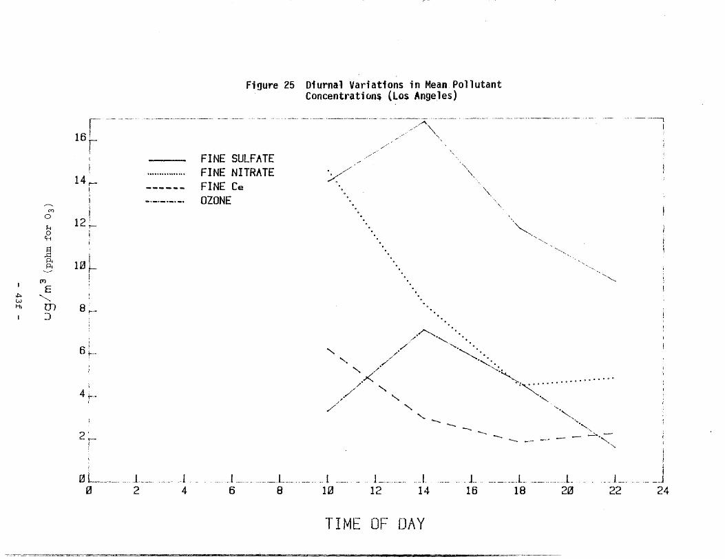
Figure 25 Diurnal Variations in Mean.Pollutant Concentratiorii (Los Ange,les)

r-- /A.'\_ . ---------~ --·-- --· ---~-· .. ·------· --··· -- . -- --- - -·----,.

l

16 ! '-,

r FINE SULFATE

,.,,-·

14 t-· I

FINE NITRATE FINE Ce

. ./-·

1/. "\,_

·,'\ __

' I OZONE ,, (Y)

0

H 0

G--t

i 12~

j ·,

......... .....

.§ Pi Pi 10~

... _ ',.

(T} ! ....'-....

E .i::. w '-----.. Ha m

:.) 8 ~-

./'-,.

BL.

I

' / .

,/

/ '- '- .,(.✓

,I' '·--... •••........__ · .. ......... ....... ·. ....... ·.

'·· .. ~'"'(_· •••••••

4~ i

2~ i

/./

,.

/✓ 0 '- '- '-

'-

-.... -..... -.... ..._ -..... .__ -··

'·

-•··

'· '-,·,., ' -- ---"• ..._

- ",

i

0 l .. __ j _____ . J - - J ______________L ___ _ -· .1 ··--· . - ... j .... I . .L . _________ L ----- ___ .L . . -.. J ___ . . ·--I

_J 0 2 4 6 8 10 12 14 16 18 20 22 24

TIME OF DAY ::.b-----....:J:..L..i_.,_ ~ ...w........ ........._____,

'F!i,.gure 26

MASS COMPARISONS 1982 ARB VISIBILITY STUDY

lSfJ r I /

i / /

125~ / I

I ~ / +} 1ool

+

+ +

+ ++ ♦

+

+

~I

U1 I

(/) I I'✓ ' ,< j I e-· ~

t4 75i­ I ,W i /

_J i t.J t

• I +t-1 ii-0::: +ssL /

I

t.0*•I + +

CL < I I+ + + +\

... .,,.,*♦ ..._._I ♦ ♦ .,,At, + -F ♦ ....,.w z / ++# ♦ t--t + 1/ .....+ ...

25! / / ~,.LL r /+ ~·· + •♦ ♦~-;It♦ +I+ r + +,.J;>'+ +

( / +.,,..... 0 ~-1+ I I __l-~-~- I I .. J_.

0 25 S0 75 ll!e 125 15S 175 200

TOTAL PARTICULATE MASS (ug/m~

NASS1V2SYMBOL•+ LINETYPE•---f;.i~">< as:e. 5417 ••s:3. 1600 b-8.4735 e,,a:8."317 •,..•13. 6868 ra=e. 8242

( r = 0.82). Higher correlation cannot generally be exnected since

the proportion of coarse particles can vary with meteorological

conditions. On average, the fine fraction represented about half

of the total particulate mass.

The proportion of the total sulfate which was in the fine fraction

was assessed in similar manner (Figure Z7) • More than 90% of the

total sulfate collected with Teflon filters was in the fine

fraction. Thus either fine or total -particulate sulfate could be

employed for data analysis in assessing contributors to light

scattering. With nitrate, however, a substantially larger fraction

of coarse nitrate was observed. Linear regression between fine and

total particulate nitrate yielded the equation:

Fine N03- • -0.625 + o.620 (Total N03-)

m 0.917

Thus nearly 40~ of the nitrate was coarse material.

Samples collected on pre-fired Pallflex quartz 2500QAO fil tars

following a cyclone (outpoint about 2.5 um) were compared for total

carbon retained to that on pre-fired glass fiber fil tars using a

conventional hi-vol sampler. The face velocities for the two

units were nearly identical (49 cm/sec for the fine particle

sampler, 47 cm/sec for the hi-vol). Assuming no significant

difference in carbon retention by the quartz and glass fiber

fil tars, differences reflect directly the proportion of carbon in

the fine fraction.

For ten paired samples collected in Riverside and downtown Los

Angeles the fine fraction carbon (ug/m3) averaged 62 ± 13% of that

in the· total particulate (hi-vol) sample. Linear regression

yielded the result:

Fine C = -3.93 + 0.789 (Total C)

- 44 -

Figure 27 Comparison of Fine and Total Particulate Sulfate

···--····•~

40_

+ s. J. ◊ RV

35_ 0 L.A. f;;' E ...,~ en 30_ :)

'-' t .,..

a 25_tn

, CJ.,_,.. 20_ f--0:: < CL 15-.. w z ........ LL 10_

y = 0.691 + 0.929x r = 0.995

5_

.0 J,t

__ ... .1 J . J. 1 l l l J

!

?t:0 5 10 15 20 b..,J 30 35 40 45

D RTT~i _ TOT f.L. , A ~ c. S04 (· ·o/m-r,~-; I. ,,

.,,,,.,.,

- 44a -

The results for percent fine carbon compare to the range 56 to 66%

obtained with dichotomous samplers at three sites.

Precedin~ results suggested that the proportion of coarse particle

carbon obtained with dichotomous sampler may be erroneously high

because of the relatively low face velocity for the coarse particle

filter (34). The present data fail to support this. The

proportion of C in the fine fraction can be assessed from Figuree

28 which "?lots fine against total Ce. The results are highly

correlated and indicate about 20% of the elemental carbon to be in

the coarse fraction. The fine Ce is compared to the total carbon,

measured by combustion in Figure 29. The results suggest, on

average, about 18% of the total carbon to be elemental carbon.

Figures 30 and 31 test linear regressions between fine particle C ,e

fine and total suspended particle mass, respectively. The moderate

correlations observed (r = 0.69 - 0.73) suggests that elemental

carbon represented about 6% of the fine particle mass.

Eo Calculated vs. Observed Ammonium Ion Levels

If one assumes all fine particle S0 4 = to be ( NH 4 ) 2S0 4 and true,

fine particle nitrate to be NH'4,N'03, then expected concentrations of

NH 4 + can be calculated. Regression equations relating observed and

calculated NH 4 values are as follows:

San Jose Cale. NH4 +

= 1.66 + 1.77 (obs. NH 4+) r = 0.81

Riverside Cale. NHt+ + = 2. 56 + o. 96 (obs. NH 4

+) r = 0.96

+ +Los Angeles Cale. NH4 = 3.92 + 0.98 (obs. NHt+ ) r = O. 95

In all cases, calculated values exceed observed values. At

Riverside and Los Angeles where high correlations were observed,

the difference was relatively constant at 2.5 to 4 µg/m 3 • This

- 45 -

1--== ~-:,.

Figure 28 Comparison of Fine and Total Particulate Elemental Carbon

12 -----~-- ------· --·---·------------ ....... --- ---------------·----·-

11

/"',.. (T)

E '-.. m :)

'-.../

c./J'

10

9

8

7

6

5

4 ---

3

2

+ s. J. ◊ RV o L.A.

◊

0

j I

J ...... L L .. L .. L. 1 ... L ... J ... L .. _L .. .L.... L ...L_J 2 3 4 5 6 7 8 9 10 11 12 13 14 15

CARBON SYMBOL=·

I LINETYPE= ---------it.W y=a+b*xg1 i--I < n=l06

_J a=0.0441 s.==0. 0421 :::J b=0. 7977 s-.==0. 0109u 81-•c0. 2685 r~0.9904 ~

t-c~ < o_

LLJ z ..........« LL

TOTAL PARTICULATE Ce (ug/m~

Figure 29 Fine Elemental Carbon vs. Total Carbon in 4-Hour Samples

VISIBILITY STUDY ,·-·-- ·--··-··-----•-·•-·· -•-·· ----

0

1 ·7l 10~

,-·I + s. J. .-,·'

◊ RV /

I /o L.A. /

l l ! ,.

/

~~·...

~ ~"1(,'i, /

~'i,v, ,/CD ), /L

~o,,V-'o, /'·, /C) /=1 ./ '--' ✓•

~ 0, 6~ / tr I

llJ u lJJ z 4t----, LL

/ .,..... +

/ /

-o,..,. /~ .A ...e (:)V.• E) y = -0.924 + 0~1aox.,...,,5 + + e

r = 0.84 0 / ee/◊ -,,,.• ❖ +

,..--l:) ◊ + e e / ◊◊ ◊

/ ◊:~~◊◊ 2 ~- / e 1¢,

✓• ◊ +·- + s ◊

◊ ◊

i /+

0 L- .,.¥..~~ .._ ~----- ◊. ...1___________________ ...L--'- ____________ - __, - j__________________ -------·-·•·-.J~ 0 10 20 30 40 so

TOTAL CARBON (UG/M3)

'""I

Figure 30 Fine Particle Mass vs. Fine Particle Elemental Carbon

--- --- ··- --------- ----A -------~- --·--·-----·--··-·:-

11 +

10 + I ·------ -·•- --- ----- ------------------I I

9 +

8 + I

---- ---- . -- ·----- ----- ··- ---------------

7 +

6..,..Fine C e

I

Iii::. (µg/m3} . I -l.11 () 5 +

4 + I•··· -

3 +

•I 2 +

II-.

A l +

. - ----·v•AA~AA

- ---- --

A A A

-- .

A

A

A A

A A

A A

--- - ------------- A ---------- ---------------~------

A

A ---·

A

B y = 0.008 + 0.0568x

A AB A A . A----A------- -------- -------•---------------------A----

A · - - r = 0 .69

___.. -A---------------------·--------------------

A A A A A

A BB A .. - AA- --- -------A--------------------·--------------··-····-------------A A

A A A

I ... ~BA~B AI A

0 ·---- --- ----- A - - ··-·- . /.. ---- -- -- -- --- - ...

-+-------+-------+-------+-------➔ -------+-------+-------+-------+-------+-------+-------+-------+-------+-----~ O 10 20 30 40 50 60 70 60 90 100 110 120 130

Fine Particle Mass (µg/m 3)

Figure 31 Total Particle Mass vs. Fine Particle Elemental Carbon

A I.. -----------------------A-----

~o•I

A

-11 +

9 +

ti Pi

Fine C e

(µg/m3)

El

7

6

~

4

3

2

1

0

+ I

I... +

A

+ --

-----A---·-- - -- -•. - -----------+

A -- -----------A------------- ---- -----

A A A + A BA

- -·----- . A - -A

A A + ----- - -- --- -------------A------¥----~O..-S94--i---0....-O-l3-7-x----- --- --

A AAB A A A A r = 0. 732A

A - --B ... A--A--AA-- --A- -- . --- A-------------. --- --- - - ---- --- --- -- --- --- -· .. + A A

A.~ A A A A - -- A-.-----·-----------···---- -----A------·•·· ----------- -------------·-··--

A A + A AA

A A

A +-

-+----+----+----+----+----+----+----+----+----+----+----+----+----+----+----+----+----+----+----+----+----+---O 10 20 30 40 50 60 70 80 90 100 110 120 130 140 150 160 170 180 190 200 210

Total Particulate Mass (µg/m 3)

(

difference may be indicative of acidic aerosols although other

cations besides NH4+ and H+ may be significant.

F. True ~article Carbon (PC) and Total Low Volatility Carbon (LVC)

Figure 32 compares total results for quartz filter samples

collected with a preceding Al 2o3 -coated denuder (sampler 4)

against total carbon results without the denuder. The results show

about 17% less carbon on the filter with the denuder, which might

infer that a corresponding amount of carbon was retained in the

denuder of sam-pler 4. However, this assumes that the presence of

the denuder does not influence the loss of carbon from the filter

by volatilization. If the denuder does remove vapor-phase,

material in equilibrium with material in particle phase, then

volatilization could be enhanced, decreasing retention of carbon on

the filter.

As discussed in Appendix F, water retained bv the A.1 203 and its

subsequent elution with CH2Cl2 - MeOH appeared to g.reatly decrease

the precision of the subsequent carbon measurements. In contrast to

prior work using CH 2Cl 2 alone for elution (40) tests of the

consistency of these results with those from other carbon

measurements have caused us to reject these data from further

analysis. Accordingly, no PC and LVC data can be considered.

G. Atmospheric Nitric Acid

I t has been prop o s e d and demons t rat e d ( 5 3 , 5 4 ) t h a t t h e

concentrations of atmospheric HN0 3 and NH 3 can be influenced by the

equilibrium:

The dissociation constant is strongly dependent on temperature. At

relative humidities below that needed to cause NH 4N0 3 to deliquesce,

- 46 -

Cua/ m3)

Figure 32 Comparison of Filter Collected Carbon With and Without 30 ·--· ··-- ___ :_______ Di_~~~~ i o~- ~~~-u~~r _!o~-~~-~~on_a._~-~-o~s _y a~~_rs _.. .. .. . ... .. _

I I-

a ___ _

-

( -;;" e

' m ::) ~

25_

~

20_

+ ◊ 0

s. J. RV L.A.

◊

A

'°'llJ I

r""Y'.... w r-·-_j,__. LL

~

15_

~

a: w _J CL ~ ·<v'1 r--lJ

... 5_

... y

r = =

0.691 0.995

+ 0.929x

J.. l . 1 L L. l 1a

l J i. L,. 15

1 ! • 1. 2C

l l . 1 1 i L.i 32

..,_J

- 46a -

a knowledge of the temperature and corresponding dissociation

constant, together with the ~H3 level, should permit calculation of

the corresponding equilibrium values for the HNO 3• Employing

reported values for the temperature dependent dissociation constant

(54), and 4-hour average measurements of NH 3 and temperature,

observed and calculated HN03 were compared. Observed HN0 3 values at

San Jose, Riverside and Los Angeles, measured by the denuder

difference technique (21), ranged from 0.25 to 8.5, 0.5 to 16.5 and

1 to 60 µg/m 3, respectively. However, only at San .Jose was a

significant correlation observed (r =- 0.73) between calculated and

observed values. The corresponding regression equation was:

- 47 -