Report Emissions Reductions by 2050 Dislocations to Significant … · 2008-08-18 · Climate Risk Industrial Constraints and Dislocations to Significant Emissions Reductions by 2050

�

Climate Risk

Industrial Constraints and Dislocations to Significant Emissions Reductions by 2050

Climate Risk Pty Ltd provides specialist professional services to business and government on risk, opportunity and adaptation to climate change.


www.climaterisk.net

A C

limat

e R

isk

Rep

ort

Climate Risk

A report commissioned by WWF-Australia

Climate Risk Pty Limited (Australia)

Sydney: + 6� 2 8006 �320

Brisbane: + 6� 7 3368 2902

www.climaterisk.net

Climate Risk Europe Limited

Manchester: + 44 �6 �273 2474

This report was prepared by:

Dr Karl Mallon BSc PhD

[email protected]

Dr. Mark Hughes

[email protected]

Design and layout by Bethan Burton BSc

[email protected]

Industrial Constraints and Dislocations to Significant Emissions Reductions by 2050. Version 1.0

This report was commissioned by:

WWF-AustraliaLevel �3, 235 Jones StreetUltimo NSW 2007Tel �800 032 55�Fax 02 928� �060

ISBN: 978-0-9804343-4-7

Disclaimer:While every effort has been made to ensure that this document and the sources of information used here are free of error, the authors: Are not responsible, or liable for, the accuracy, currency and reliability of any information provided in this publication; Make no express or implied representation of warranty that any estimate of forecast will be achieved or that any statement as to the future matters contained in this publication will prove correct; Expressly disclaim any and all liability arising from the information contained in this report including, without limitation, errors in, or omissions contained in the information; Except so far as liability under any statute cannot be excluded, accept no responsibility arising in any way from errors in, or omissions contained in the information; Do not represent that they apply any expertise on behalf of the reader or any other interested party; Accept no liability for any loss or damage suffered by any person as a result of that person, of any other person, placing any reliance on the contents of this publication; Assume no duty of disclosure or fiduciary duty to any party. Climate Risk support a constructive dialogue about the ideas and concepts contained herein.

© Copyright Climate Risk Pty Ltd, 2008 This document is protected by copyright. Consent is given to reproduction from this document provided Climate Risk Pty Ltd is acknowledged in writing and the Climate Risk Pty Ltd logo is attached to any diagrams which are reproduced.

Dr. Karl Mallon

Dr. Karl Mallon is director of Science and Systems at Climate Risk Pty Ltd. He is a First Class Honours graduate in Physics and holds a Doctorate in Mechanical Engineering from the University of Melbourne. Karl has worked in climate change and energy since 1991, and is the editor and co-author of ‘Renewable Energy Policy and Politics: A Handbook for Decision Making’ published by Earthscan (London). He has worked as a technology and energy policy analyst for various international government and non-government organisations since 1997. As an invited expert consultant, he participated in the World Bank Extractive Industries Review. Karl has been a member of the CSIRO’s Energy Futures Forum that reported in 2006, as well as a director of the Australian Wind Energy Association between 2003 and 2005.

Dr. Mark Hughes

Dr. Mark Hughes is a first class honours graduate in Materials Engineering and holds a doctorate in Materials Science from the University of Cambridge. He has been the recipient of research scholarships from the Cambridge Commonwealth Trust, The British Government and the Oppenheimer Trust. Mark has also been awarded fellowships with the Chevening Technology Enterprise Program (London Business School) and Darwin College (University of Cambridge). Since 1999, he has been based in the field of energy storage and the environment, and is author of a range of peer-reviewed publications in internationally distributed journals. Mark has also worked on commercialisation and fund raising for new technologies emerging in the energy sector.

Climate Risk Team

Climate Risk acknowledges the contribution of Martin Raynor to this report.

Dr. Hugh Saddler

Dr Saddler has a degree in science from Adelaide University and a PhD from Cambridge

University. He is the author of a book on Australian energy policy, ‘Energy in Australia’

and over 50 scientific papers, monographs and articles on energy technology and

environmental policy, and is recognised as one of Australia’s leading experts in this field.

He is currently a member of the Experts Group on Emissions Trading, appointed by the

Australian Greenhouse Office, of the ABS Environmental Statistics Advisory Group, and

of the ACT Environment Advisory Committee. In 1998 he was appointed an Adjunct

Professor at Murdoch University. He is a Fellow of the Australian Institute of Energy and a

member of the International Association for Energy Economics. Between 1991 and 1995 he was a member of

the Board of the ACT Electricity and Water Authority. In 1995 he was a member of the Expert Selection Panel

for the 1995 Special Round of the Cooperative Research Centres Program (renewable energy technologies).

Dr. Robin Roy

Dr. Robin Roy has over two decades of experience in the energy sector in the U.S.

and Australia. Over the last ten years, he has undertaken a wide variety of public and

private sector consulting assignments in the Australian utilities sector. Robin was

formerly Project Director & Fellow at the United States Congress’ Office of Technology

Assessment where he advised the Congress on competition in the electricity market,

energy efficiency initiatives and nuclear industry issues. Prior to that, he was with Pacific

Gas and Electric Company in their strategic planning group. Dr Roy gained a Ph.D., MS

and BS from Stanford University..

Peer Reviewers

Climate change is the greatest threat facing our nation and our planet. Scientific analysis indicates we

must limit the rise in global average surface temperature to less than 2 degrees above pre-industrial

levels if we are to avoid dangerous impacts on nature, humans and the global economy.

Recent evidence suggests global greenhouse gas emissions are much higher than previously thought.

This is bad news for Australia, which is particularly vulnerable to climate change.

As a rich and high-emitting nation, Australia has a responsibility to display leadership. We must act

now to stabilise emissions and then cut them significantly.

The implementation of an emissions trading scheme by 20�0 is a critical step to achieve the

necessary emissions reductions. However the report Industrial Constraints to Emissions Reductions,

commissioned by WWF, shows that an emission trading scheme on its own is not enough. There is

a need for a specific industry deployment scheme like the Renewable Energy Target to facilitate the

timely and well-managed deployment of a range of low emission technologies, particularly if Australia

has to tighten its emissions reductions target in the future.

The report shows that the technologies and sustainable energy resources available today or reasonably

in prospect are sufficient to meet the climate change challenge. It is now imperative to ensure that

these technologies are deployed quickly and that flexibility and resilience is built into the emission

reduction system.

Not to decide to win is to decide to fail.

Greg Bourne

CEO WWF-Australia

Foreword

Part 1

� Executive Summary �1.1 Introduction 11.2 The Model 21.3 Outputs 21.4 Findings 31.5 Conclusion 6

Part 2

2 Methodology 7

Part 3

3 Plausible Future Emissions Levels 93.1 Business-as-Usual 93.2 Rudd Government Targets 103.3 Target-Taker versus Target-Setter 103.4 International Negotiations 113.5 United States of America 113.6 The European Union 11

Part 4

4 Description of the Industrial Growth Model �54.1 Key Features of the Model 15

Part 5

5 Scenario Results 255.1 Rudd Government Scenario 265.2 US Candidates’ Equivalent Scenario 285.3 European Union Equivalent Scenario 305.4 Sequential Uptake Scenario 325.5 Dual Carbon Budget (Late Tightening) Scenario 34

Contents

Part 6

6 Findings: Constraints and Dislocation Risks 376.1 System Inertia: Late Start Risks 376.2 Development Time and Industrial Growth Rate Constraints 386.3 Industrial Skills Shortage 396.6 Late Target Re-Setting 436.7 Irreducible Emissions 446.8 Energy Management and Conversion Constraints 446.9 Sequestration Infrastructure 456.10 Learning Rate Retardation 456.11 Transport Fuel Supply 456.12 Energy Based Community Location Changes 466.13 Major Load Location Changes 466.14 Supportive Planning 466.15 Agricultural Activities 476.16 Ad Hoc Low-Carbon Policies Will Create Stranded Assets 476.17 Productivity and Risk 48

7 References 498 Glossary 5�9 Appendix: Scenario Settings and Outputs 54�� Appendix: Matrix of Key Model Inputs 63�2 Appendix: Table of Existing and Proposed Fossil Fuel Power Plants 64�3 Appendix: Sustainable Industry Growth Rates 68

�

Climate Risk


1 Executive Summary

1.1 Overview

The objective of this project was to identify industrial constraints to achieving national greenhouse gas emissions reductions of 60%-90% below �990 levels by 2050. Emissions reductions of 60% are required by the Rudd Government’s climate change policy. Emissions reductions of 80%-90% in Australia are consistent with emissions reductions proposed by political leaders in the United States of America and the European Union, and therefore it is foreseeable that reductions of that magnitude may be required at some point in the future.

The project complements economic modelling by analysing physical industrial constraints such as the availability of skilled personnel (such as engineers, technicians, trades, project managers and lawyers), production equipment and materials (whether raw, component or finished).

The project analyses physical industrial constraints by using a computer-based model to calculate the rates at which low emission technology and service industries need to grow to provide energy and other commodities required by an increasing population while attaining greenhouse gas emissions reductions of 60%, 80% and 90% respectively, by 2050. The model then compares that output with the findings

of international industrial development literature. This literature suggests that industry growth rates of more than 20% per year are possible, though difficult to achieve year on year, but that industry growth rates of more than 30% per year are generally unsustainable (the most common exception being growth rates achieved by small fast moving electronic consumer items like mobile phones and consumer electronics).

The key constraint is the need to achieve the reductions by 2050. It is probable that, without the need to achieve the emissions reductions by that date, and assuming that greenhouse gas emissions are “priced”, the market alone would be sufficient to achieve deep emissions reductions but over a longer period.

The modelling finds that there are sufficient low emission energy resources, energy efficiency opportunities and emissions reduction opportunities in non-energy sectors to achieve reductions of 60%-80%, and even emissions reductions of 90% or more if livestock emissions are reduced; and that there is sufficient time for the low emission technologies and services to grow at sustainable rates if development starts promptly. The model finds that a sequential approach to low emission industry development (lowest-cost technology first, next-lowest-cost technology next and so on) requires much higher growth rates for each industry than one that grows

Part 1

The central constraint on delivering the low emission options in the period to 2050 is the time required to permit stable growth of the industries which will deploy the required technologies and services.

2

Climate Risk


a number of technologies/industries concurrently.

The modelling finds that physical industrial constraints will not prevent Australia reducing greenhouse gas emissions of 60% by 2050, though doing so will be made less demanding if a broad range of low emission industries are fostered from the outset.

The modelling also finds that emissions reductions beyond 60% cannot be achieved using a sequential approach to low emission industry development without pushing industries to implausibly high levels of annual growth. If emissions reductions of beyond 60% are required, a concurrent approach to low emission industry development is essential. In particular, the “dual carbon budget” proposed by the Garnaut Climate Change Review (whereby Australia offers to make deeper cuts if other countries do likewise) is very vulnerable to failure due to industrial growth constraints. However, this can be overcome by promptly and concurrently fostering a wide suite of low emission technologies and industries.

Technology-neutral policy mechanisms such as emissions trading schemes and

the Renewable Energy Target generally result in the sequential development of low emission industries. However, they can foster concurrent development if less than 20% of the revenue from an emissions trading scheme is used to support a range of low emission technologies/industries (such as renewables, CCS, agriculture) until they are competitive in the market or if industry development schemes such as the Renewable Energy Target are strengthened by being banded as proposed below.

Other findings of the project are that deep reductions can only be achieved if Carbon Capture and Storage (CCS) is used to capture industrial process emissions (including from iron and steel, cement).

Table �. The table shows that the peak growh rates are much higher if industries are not developed concurrently.

Industrial growth rate toreduce emissions by 60%

Industrial growth rate toreduce emissions by 80%

Sequential approach Requires 28% per year Requires 55 % per year

Concurrent approach Requires 20% per year Requires 25 % per year

Figure �. The comparison between prompt concurrent industry development and a sequential uptake policy framework becomes more stark for emissions reductions targets deeper that 60%. In this case growth rates are much higher than a plausible upper limit of about 30% per year. Consequently it is fair to conclude the option of emissions cuts deeper than 60% may be undeliverable by ‘industry neutral’ policy frameworks.

30

20

10

0

60

50

40

Emissions reductionof 60% (Rudd)

Emissions reductionof 80% (US)

Sequential

Concurrent

Ind

ust

ry g

row

th r

ate

(%)

3

Climate Risk


The model finds that the existing Renewable Energy Target scheme, or a similar industry deployment scheme, is an essential element of the national response to climate change. The model also finds that the Renewable Energy Target scheme could be made more sustainable, in industrial growth terms, by “banding” or quarantining proportions of the scheme to foster the growth of the important resources such as geothermal, solar photovoltaics and solar thermal industries from the commencement of the scheme. These are all industries in which Australia is likely to have a strong resource or comparative advantage. Biomass, another low emission industry in which Australia is likely to have a strong comparative advantage, should be able to compete under the Renewable Energy Target scheme without further assistance.

The modelling indicates that the Productivity Commission’s opinion that the Renewable Energy Target scheme operating in conjunction with an emissions trading scheme would not encourage any additional abatement but would rather impose unnecessary administration and monitoring costs� is incorrect. Instead the results indicate that the Renewable Energy Target scheme effectively manages the risks associated with a change in national emission reduction target and the failure or underperformance of one or more low emission technologies. The modelling also indicates that the rate of industrial growth is likely to be more sustainable in circumstances where a range of low emissions industries are

fostered concurrently. Thus, although the Renewable Energy Target scheme does not provide any additional abatement in the medium-term, it positions the country to achieve deeper reductions should they be required in the longer-term (as is likely, given the US and European position, to be the case) and provides the Government’s emission reduction system with desirable resilience against the failure of one or more low emission technologies. In some respects this is an example of a wider issue in modern, open economies which, though highly efficient in the allocation of the resources, often undervalue the consequences of unusual but not unforeseeable events. The explosions of the gas plants at Varanus Island, Western Australia on 3 June 2008, which disrupted 30%-40% of Western Australia’s domestic gas supply, and at Longford, Victoria on 25 September �998, which affected 4 million people and cost industry $�,300,000,000, are two good examples of a lack of resilience to unusual but not unforeseeable events. Lack of resilience is particularly important in the case of energy, which performs a function in terms of productivity not necessarily accurately represented in national accounts, and attains even greater importance in the case of low emission technologies where the political, environmental and ultimately economic consequences of failing to achieve emission reduction targets could be severe.

� Submission to Garnaut Climate Change Review.

4

Climate Risk


1.2 The Model

The report utilises a computational model that emulates real-world industrial growth. The model identifies the resources, technologies and services available to reduce greenhouse emissions (adopting the Princeton abatement “wedges” framework, Pacala & Socolow 2004) and then uses Monte Carlo methods to combine this information in order to calculate the industrial growth rates required to achieve the necessary emissions reductions while satisfying the projected demand for energy services.

Monte Carlo methods are a class of algorithms that rely on repeated random sampling to compute their results. They are often used when simulating physical systems. They allow multiple data sets and expert opinions to be used; for example, about the national abatement potential of energy efficiency or wind energy.

As noted above, the outputs of the scenarios presented in this report suggest that without targeted industry development measures, industrial growth constraints are likely to prevent significant emission reductions being achieved by 2050.

1.3 Outputs

For each of the emissions reduction scenarios modelled, the outputs of this project are:

An emissions profile of the suite of industries and services required to achieve the relevant reductions;

a)

An energy services profile; and

A suite of industrial growth rates corresponding to the delivery of this outcome.

The scenarios have been constructed to explore the industrial growth rates required to achieve the emissions level outcomes for the following policy approaches:

The Australian Government 2050 target (60% cuts by 2050);

The emissions reductions proposed by US Democrat Party Presidential candidate Senator Barak Obama (80% cuts by 2050);

The European Union policy of remaining below 2oC (cuts greater than 90% by 2050);

A “technology neutral” version of the Rudd scenario with sequential approach to large-scale deployment of low emission technologies and services; and

b)

c)

a)

b)

c)

d)

Figure 2. Comparison of abatement industry early growth rates (from �% to 20% of resource exploitation) for the three emissions reduction scenarios showing the increase significant growth rate increase required for deeper emission cuts.

15

10

5

0

35

30

25

20

Rudd Scen

ario

(60%

cut)

US Sce

nario

(80%

cut)

EU Sc

enar

io

(90%

+ cut)

Gro

wth

Rat

e (%

)

5

Climate Risk


A “dual carbon budget” approach with a change from the Rudd Government target to the US Democrat Party reduction target post 2020.

For simplicity, a single set of industrial growth rates has been applied to all abatement industries.

1.4 Findings:

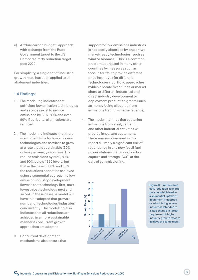
The modelling indicates that sufficient low emission technologies and services exist to reduce emissions by 60%-80% and even 90% if agricultural emissions are reduced.

The modelling indicates that there is sufficient time for low emission technologies and services to grow at a rate that is sustainable (30% or less per year, year on year) to reduce emissions by 60%, 80% and 90% below �990 levels; but that in the case of 80% and 90% the reductions cannot be achieved using a sequential approach to low emission industry development (lowest-cost technology first, next-lowest-cost technology next and so on). In these cases, a model will have to be adopted that grows a number of technologies/industries concurrently. The modelling also indicates that all reductions are achieved in a more sustainable manner if concurrent growth approaches are adopted.

Concurrent development mechanisms also ensure that

e)

�.

2.

3.

support for low emissions industries is not totally absorbed by one or two market-ready technologies (such as wind or biomass). This is a common problem addressed in many other countries by measures such as feed-in tariffs (to provide different price incentives for different technologies), portfolio approaches (which allocate fixed funds or market share to different industries) and direct industry development or deployment production grants (such as money being allocated from emissions trading scheme revenue).

The modelling finds that capturing emissions from steel, cement and other industrial activities will provide important abatement. The scenarios examined in this report all imply a significant risk of redundancy in any new fossil fuel power stations that are not carbon capture and storage (CCS) at the date of commissioning.

4.

15

10

5

0

35

30

25

20

Rudd Scen

ario

with

concu

rrent u

ptake

Rudd Scen

ario

with

sequen

tial u

ptake

Dual Car

bon

Budget Sc

enar

io

Gro

wth

Rat

e (%

)

Figure 3. For the same 60% reduction scenario, policies which lead to a sequential uptake of abatement industries or which bring in new industries later due to a step change in target require much higher industry growth rates to achieve the same result.

6

Climate Risk


Olympic Dam

Mt Isa

Olympic Dam

Mt Isa

Bell Bay

Port Pirie

Boyne

Port Henry

Nickel West

Mine sites

Smelters

Port Hedland

Fairview

Kalgoorlie

Insolation

Highest

Lowest

Fairview

Olympic Dam

Mt Isa

Olympic Dam

Mt Isa

Bell Bay

Port Pirie

Boyne

Port Henry

Nickel West

Port Hedland

Kalgoorlie

Figure 4. It may be in Australia’s strategic interests to be a supplier of low emission energy for highly energy intensive industrial processes such aluminium production. The figures show the location of large geothermal and solar thermal energy resources with locations of high energy demand and possible future energy demand for metals and minerals processing and cement production.

7

Climate Risk


2 Methodology

The modelling methodology presented in this report has been developed to consider the industrial implications of specific greenhouse gas emissions (GHG) levels to 2050 and beyond. The methodology uses both a bottom-up and top-down approach to climate mitigation modelling. This allows for consideration of abatement relative to ABARE (Australian Bureau of Agricultural and Resource Economics) business-as-usual baselines for emissions and energy (Gurney 2007) along the lines of a Socolow Wedge (Pacala & Socolow 2004) methodology, but also allows for a reality-check of these results from the ground up.

A probabilistic approach has been used which allows for ranges of data on resources, technology performance and other parameters to be included, combined and reflected in the probability distributions of final results.

The analytic method can be described by the following steps:

Step 1: Establish Future Emissions Levels

Establish a plausible carbon budget range for Australia’s emissions in 2050 by reviewing national and international commitments, and negotiating positions. This gross carbon budget can be described on either a national or per capita basis. The scenarios in

this report are defined on a per capita emissions basis to enable appropriate comparisons between various international emissions targets.

Step 2: Establish the Net Carbon Budget (Including Irreducible Emissions)

Some activities which contribute to the Australian economy have associated emissions which cannot be reduced beyond a certain limit without decreasing the causal activity (e.g. livestock or cement production). Where possible, the modelling methodology assumes that all current activities in the Australian economy are maintained through to 2050. However, in some of the more demanding scenarios, it was not possible to achieve the required emissions reductions levels without assuming some activities are curtailed. Once the “irreducible emissions” are identified and quantified, the irreducible emissions sources are pre-allocated part of the gross carbon budget. This yields a remaining net carbon budget for allocation across all the sectors of the economy.

Step 3: Establish the Baseline of Resource Requirements

Future emissions levels will be significantly determined by resource requirements and drivers, including: energy services demand, agricultural and land use activity, GDP (gross domestic product) growth, population

Part 2

8

Climate Risk


and consumption levels. These elements can be used to establish or adjust baselines, while also taking into account the effects of climate change which may, for example, impinge on agricultural and mining output and other economic activity.

Step 4: Establish Data-Sets for Relevant Industries and the Capacity for Change

Growth of low-emission industries and corresponding emissions abatement ‘wedges’ is modelled based on technological availability, national resource base and stable industrial growth rates. The relevant industries have particular extant performance and resource characteristics, which inform their potential contribution and development rates. In some cases the performance of other comparable industries has been considered. These characteristics were compiled from public domain data. Differing opinion is reflected as triangular probability distributions of the inputs (see chapter 4).

Step 5: Interpret and Inputs Driver Frameworks

Policy frameworks have an impact on the commencement point of industry development, the rates of uptake, and development dynamic. For example, a technology neutral policy mechanism (such as an emissions trading scheme) is likely to lead to a sequential development dynamic for low emission industries in which lower cost technologies develop first and more expensive options develop later.

Resource-specific policy mechanisms give rise to concurrent development dynamics in which several low emission industries develop simultaneously.

Step 6: Establish Industry Settings in the Monte Carlo Simulator

Industrial development based on the range of possible inputs established above is run repeatedly in a Monte Carlo simulation. This builds a picture of the range and probability of outcomes based on the range and probability of the inputs.

Step 7: Express Scenario Results

Results are presented in terms of industry development and deployment, energy sector make-up, non-energy sector make-up and net emissions projection.

Step 8: The Carbon Corridor, Dislocations and Industry Constraints

The net emissions trajectory combined with the emissions profile and lifetimes of existing, proposed and potential high-emissions sources, as well as irreducible emissions creates a de-facto

“Carbon Corridor”. Emissions outside this corridor will either miss the target emissions level or bring about stranded assets (i.e. assets which are retired early or remain under-utilised). Dislocations and constraints occur where stranded assets are created, industries undergo excessively rapid phase-in or phase-out, where regional impacts are concentrated, and also where major changes to essential national infrastructure are required.

9

Climate Risk


3 Plausible Future Emissions Levels

3.1 Business-as-Usual

The Australian greenhouse inventory for 2005, published in 2008, indicates that national per capita emissions are currently 27.6 tonnes carbon dioxide equivalent (tCO2-e) per year (DCC 2008a, DCC2008b). Long-term emissions projections to 2050 are available from the ABARE 2007 reference case (Gurney 2007). These are used to establish a de-facto business-as-usual outlook for the Australian economy and its interface with the international economy. In this reference case, emissions approximately double over the period from 2000 to 2050.

The key aspects of the ABARE 2007 scenario used in this modelling include

the GDP baseline, emissions baseline and energy baseline (Gurney 2007). These are shown in the following figures below. The ABARE reference case can be adjusted in the model for variations in future population, climate change impacts and wealth-consumption de-coupling.

This reference case does not include the effects of policy commitments from the Rudd Government. All of the policy commitments are included in the emissions abatement options considered in this report and the low emission industry wedges modelled. One of the most potentially significant policies may be the Australian Emissions Trading Scheme (AETS), but this has not been quantified by the Government at the time of writing this report.

Part 3

Greenhouse gas emissions Australia

Year

2010 2050204020302020

MtCO2-e

200

150

100

50

Mtoe

2010 2050204020302020

1000

800

200

400

200

Australian primary energy consumption

Year

Figure 5. Business-As-Usual projections for primary energy consumption and emissions to 2050 (ABARE, 2007).

�0

Climate Risk


3.2 Rudd Government Targets

The most significant impact on future emissions is likely to be legally binding national and/or international commitments to greenhouse gas abatement targets and/or future emissions levels.

The Rudd Government has currently committed to emissions cuts of 60% below 2000 levels by 2050. Emissions in 2000 were 55�.5 MtCO2-e (Kyoto greenhouse gases only; DCC 2005). This target therefore represents an emissions level of 2�9 MtCO2-e in 2050 and this in turn is consistent with a per capita emissions level of 7.8 tCO2-e for a population of 28 million.

3.3 Target-Taker versus Target-Setter

In this report we assume that Australia will be a recipient of international climate targets and policies, which will be driven largely by negotiations between the world’s current large economies and emerging large economies, as well as significant emitters including the European Union (EU), the USA, Russia, Japan, China, India, Brazil and Indonesia.

The trade influence of these larger economies and blocs will generally underpin their ability to leverage agreement and compliance from smaller economies and trading partners such as Australia. Strong protectionist drivers

Figure 6. Effect of Rudd Government election commitments on national emissions to 2020 (Climate Risk 2007a).

State Measures

ALP-Clean Businesses

ALP-Rental Insulation

ALP-Solar Schools

C-Efficient Lighting

ALP-ETS

ALP-MRET

ALP-Clean Coal Iniative

ALP-Domestic EE Loans

ALP-EE Govt Bldgs

ALP-Standby Efficiency

ALP-Appliance Standards

ALP-Green Car Partners

ALP-Solar Powered Homes

ALP Efficient Hot Water

Year

1990 202020152010200520001995

700

Annual EmissionsMtCO2-e pa

650

600

550

500

��

Climate Risk


have already emerged with regard to unilateral action on climate change in the EU. For example, France takes the position that trade barriers should be examined to protect industries within a low-carbon zone (NYT 2007) from imports coming out of non-carbon constrained countries (i.e. non-Kyoto/Kyoto2 participants). Such positions may portend the types of influence that could be applied to high-emission and/or non-compliant nations.

3.4 International Negotiations

Currently, a new round of UN negotiations is underway to establish commitments post-20�2, expected to be finalised in Copenhagen by late 2009. The UNFCCC COP�3 negotiations in Bali included a mandate to work towards a new round of binding emissions targets, with a reference to developed country targets of 25-40% reductions in greenhouse gas emissions by 2020 (Bloomberg 2007).

3.5 United States of America

The current US administration signed off on the Bali Mandate for negotiating the next round of post-20�2 binding emissions targets. However, the US has not ratified the Kyoto Protocol and appears unlikely to do so within the current Bush Administration.

The positions of the two current US presidential candidates are as follows (NYT 2008):

Senator John McCain supports a cap-and-trade system and co-sponsored the

Climate Stewardship and Innovation Act of 2007, to reduce carbon emissions by 30% from 2000 to 2050. He also sponsored an amendment to the Energy Policy Act of 2005, which would have capped GHG emissions at 2000 levels by 20�0. He has stated a campaign policy position of returning emissions to �990 levels by 2020 and to 60% below �990 levels by 2050 (McCain 2008).

Senator Barack Obama co-sponsored the Global Warming Pollution Reduction Act in 2007, which would require the USA to reduce emissions to 80% below �990 levels by 2050. Like Senator McCain, he co-sponsored the Climate Stewardship and Innovation Act of 2007, and supported the above-mentioned amendment to the Energy Policy Act of 2005. Senator Obama’s campaign position calls for emissions reductions of 80% by 2050, relative to �990 levels.

Thus, both candidates propose firm intervention on climate change, with emissions targets for 2050 by up to 80% below �990 levels. The 80% emissions reductions target on �990 levels would reduce US annual emissions to �,297 MtCO2-e in 2050 (with land use change, forestry and bunker fuels included; EPA 2008). Based on a projected US population of 397 million people in 2050 (ABARE 2007), commitments to 80% cuts in the USA would equate to annual per capita emissions of 3.3 tCO2-e in 2050.

3.6 The European Union

The position of the European Union, the world’s largest economic bloc, is

Based on a projected US population of 397 million people in 2050 (ABARE 2007), commitments to 80% cuts in the USA would equate to annual per capita emissions of 3.3 tCO2-e in 2050.

�2

Climate Risk


based on “avoiding dangerous climate change.” The European Parliament has stated this is consistent with avoiding a temperature increase of 2°C above pre-industrial levels (European-Council �996, European-Council 2005).

The EU has not adopted an atmospheric (parts per million [ppm]) concentration target, or an EU-wide or per capita emissions target for 2050. However, the EU has adopted a dual 2020 target of 20% reduction in emissions on �990 levels if it reduces its emissions alone, or a 30% reduction if it is part of a broader international agreement.

Figure 7 indicates that stabilising emissions in the long-term at 450 ppm provides a 50% chance of stabilising global warming below 2°C, and therefore equal chance of exceeding 2°C (Meinhausen 2006).

Preventing a temperature increase above 2°C implies reduction below 450 ppm. Current emissions in the atmosphere are estimated at 455 ppm atmospheric concentration (Meinhausen 2006). However, analysis indicated that the effect of biosphere and ocean absorption does make a long-term sub-450ppm stabilisation possible (Meinhausen 2006).

In order to calculate a per capita emissions level associated with the EU position, Meinhausen’s analysis indicates that a stabilisation at 400ppm has a 74% chance of avoiding a warming increase of greater than 2 degrees. Though this still leaves a 26% chance that this temperature will be breached. This appears to be the lower end of current plausible emissions stabilisations presented in the literature. Meinhausen estimates that stabilisation

Figure 7. Stabilising emissions in the long-term at 450 ppm provides a 50% chance of stabilising global warming below 2°C, and therefore equal chance of exceeding 2°C (Menihausen, 2006).

20001900 2100 2200 2300 20001900 2100 2200 2300 20001900 2100 2200 2300 2400

Tem

per

atu

re a

bo

ve p

re-i

nd

ust

rial

Year

+7oC

+6oC

+5oC

+4oC

+3oC

+2oC

+1oC

+0oC

550 450 400

84%Risk

52%Risk

26%Risk

1%

9%

23%

33%

23%

9%

1%

9%

23%

33%

23%

9%

1%

1%

9%

23%

33%

23%

9%

1%

+2oC

�3

Climate Risk


at 400ppm CO2-e requires an emissions cut of 55% from �990 levels by 2050 (Meinhausen 2006) . Assuming global emissions in �990 were 42,000 MtCO2-e per year, a 55% reduction would leave annual emissions at approximately �9,000 MtCO2-e in 2050, or 2.� tCO2-e per person per year.

Alternatively, the IPCC Fourth Assessment Report Working Group 3 indicates that a temperature range of 2.0-2.4 degrees is consistent with global GHG emission reductions of 85% to 50% below 2000 levels (IPCC 2007). Global emissions in 2000 (including land use change, forestry and bunker fuels) were 44,000 MtCO2-e. Thus the 85% and 50% reduction figures translate into reducing annual emissions levels to a level of between 6,650 and 22,�70 MtCO2-e. Based on a projected global population of 9 billion in 2050 (UNPP 2006), this would be consistent with per capita annual emissions levels of 0.74 tCO2-e and 2.4 tCO2-e, respectively, per year in 2050. Though these figures are based on probability distributions, staying below 450 ppm implies per capita emissions at or below the bottom of this range.

Baer and Mastrandrea estimate that sub-370ppm emissions of carbon dioxide (not CO2-e) would require emissions reductions of 7�-8�% on �990 levels by 2�00. These have not been used in this report as it is unclear whether

this emissions level constitutes a stabilisation.

In this report we assume the EU position on annual per capita emissions to be somewhere between 0.74 tCO2-e and 2.4 tCO2-e, from which we have selected a per capita emissions level of �.6 tCO2-e/yr in 2050 to be used for the EU scenario.

�4

Climate Risk


�5

Climate Risk


4 Description of the Industrial Growth Model

4.1 Key Features of the Model

4.1.1 All Major Emission Sectors

The model includes all major emissions sectors including stationary energy, industrial processes, transport, land use and land use change, forestry, waste, agricultural emissions, as well as fugitive emissions. This allows a side by side comparison of the scale of different abatement options, though no preference or order of implementation is implied.

4.1.2 Commercially Available Industry Forcing

The Model is therefore primarily an ‘industrial model’ rather than an ‘economic model’; price and cost have not been used to limit or guide the uptake of technologies. The model works from the point of view of the emissions outcome being fixed as an input, with the consequences for industrial development being an output. By forcing industries to deliver the required emissions outcomes which are set as inputs, the plausibility of output growth rates and other real world constraints can be considered.

4.1.3 Resource and Technology Options

Only emission abatement technologies which are commercially available, or likely to be in the near term, have been included. The Model is able to look at price shortfalls between included technologies and business as usual, as well as with the inclusion of carbon prices. And, with rational learning rates, the modelling indicates that all the technologies identified would be able to compete openly in a market with anticipated carbon costs by 2050. However, cost behaviour is not the focus of this report, but may be the subject of subsequent publications.

4.1.4 Extending the Pacala-Socolow ‘Wedges’ Concept

A considerable amount of modelling has been undertaken in the fields of both climate change and energy. Many models are constructed in ways that let scenarios evolve based on costs, such as the price of oil or the cost of carbon.

A “wedges” model, developed by Pacala and Socolow (Pacala & Socolow 2004) is widely viewed as an elegant approach to considering and presenting the means of achieving future greenhouse gas emissions levels and provides an excellent starting point. It divides the task of emissions stabilisation over 50 years into a set of seven “wedges” (delivered by emissions-avoiding technologies) each of which grows, from a very small contribution today, to a

Part 4

�6

Climate Risk


Carbon Corridor

0.00E+00

2.00E+05

4.00E+05

6.00E+05

8.00E+05

1.00E+06

1.20E+06

1.40E+06

1.60E+06

1.80E+06

2.00E+06

2008 2018 2028 2038 2048

Fina

lEne

rgy

Serv

ices

(GW

h/yr

)

Industrial Energy Efficiency (Non-M etals)M etals Energy EfficiencyEfficient buildingsEfficient vehiclesReduced use of vehiclesAviation and shipping efficiencyAvoided AviationBio-HydroCarbonsSea and Ocean EnergyDomestic Solar ThermalBuilding Integrated Solar PVSolar Power StationsGeothermalWind powerSmall HydroRepowering Large Hydro

Fossil with CCSResidual EmissionsPlanned Other Fossil Fuel Power StationsPlanned Gas Power StationsPlanned Coal Power StationsExisting Other Fossil Fuel Power StationsExisting Gas Power StationsExisting Coal Power Stations

Existing Large Hydro

Year

2010

Fin

al E

ner

gy

Serv

ices

(G

WH

/yea

r)

0.0E+00

2.0E+05

4.0E+05

6.0E+05

8.0E+05

1.0E+06

1.2E+06

1.4E+06

1.6E+06

1.8E+06

2.0E+06

2020 2030 20502040

Year

2010

Emis

sio

ns

and

avo

ided

em

issi

on

s (G

tCO

2-e/

yr)

FugitiveWasteForestryLULUCAgricultureIndustrial Energy Efficiency (Non-M etals)M etals Energy EfficiencyEfficient buildingsEfficient vehiclesReduced use of vehiclesAviation and shipping efficiencyAvoided AviationBio-HydroCarbonsSea and Ocean EnergyDomestic Solar ThermalBuilding Integrated Solar PVSolar Power StationsGeothermalWind powerSmall HydroRepowering Large HydroFossil with CCSResidual EmissionsPlanned Other Fossil Fuel Power StationsPlanned Gas Power StationsPlanned Coal Power StationsExisting Other Fossil Fuel Power StationsExisting Gas Power StationsExisting Coal Power StationsIrreducible Emissions

2020 2030 20502040

0.1

0.3

0.2

0

0.4

0.5

0.7

0.9

0.8

0.6

Net CarbonBudget

IrreducibleEmissions

Gross Carbon Budget

Scenario SettingsIndustry Data

Monte Carlo Simulator

Carbon Budgets

EmissionLevel

Population Consumption PolicyFrameworks

Climate Change Impacts

Baseline ResourceRequirements

Market Dynamics

ImplementationTiming

Learning Rates

BAU Fuel PriceProjections andPrice RiskProjections

ExistingInfrastructureCommitmentssize, production,commissioned,life-time,financing period,emission intensity

Industry and Resource Optionsresource volumes,installed capacity,starting costs,capacity factor,learning rates

Scenario Outputs (Histograms)• Emissions• Energy• Non-energy• Industry Allocation

Industry Settingsgrowth dynamics

Industry1

Industry2

Industry3

Industry4

Industrygas

Industryccs

Industrypower management

Industrysynthetic energy carriers

Annualised Output and ProbabilityDistribution for Each Industry

Some areInterdependent

Emission Projection Energy Projection

• • •

Carbon Corridor

Figure 8. Schematic diagram of the industry allocation model.

�7

Climate Risk


point where it is avoiding the emission of � gigatonne of carbon per year by 2050. Its authors point out that many more of these “wedges” are technically available than are required for the task of stabilising global emissions at today’s levels by 2050.

The Model presented herein builds on the Pacala-Socolow “wedges” model by adapting it to go beyond stabilisation of emissions in 2050, to achieve reductions in global emissions consistent with the current Rudd government position, that of the US Democratic candidate and that of the European Union. In order to do this, the Model:

Extends the penetration of abatement industry deployment so as to achieve abatement consistent with plausible future carbon budgets.

Models real world industrial growth behaviour by assuming: that the growth of any technology will follow a typical sigmoid (S-shaped) trajectory; that constraints impose a maximum on the rate of sustainable growth; and that the ultimate scale depends on estimated resources and other specific constraints.

Draws on a diversity of expert opinions on the potential size and scale of emissions abatement resources as inputs to the model.

Employs a probabilistic approach using the ‘Monte Carlo’ computational methods so that

�.

2.

3.

4.

the results can be considered as probabilities of achieving certain outcomes or risks of failure.

Seeks to minimize the replacement of any stock or system before the end of its physical or economic life.

Includes energy and emissions contingencies which allows for the possibility that some solutions may encounter significant barriers to development and therefore fail to meet the projections set out in the model.

4.1.5 Top-down and Bottom-up

The model combines top-down and bottom-up aspects of emission abatement analysis to capture the best of both ends of the debate regarding how best to approach future emissions cuts – the global requirement for energy and abatement opportunities (“top down”) and the development of options for meeting these needs (“bottom up”).

The top-down aspect of the model has as its starting point ABARE’s baselines for GDP, energy and emissions out to 2050 (Gurney 2007). However, top-down approaches can introduce perversities such as inflated baselines which create the illusion of greater emissions reduction than is possible. The bottom-up aspect of the model builds a set of abatement industries to meet the projected energy services demand, sector by sector. This requires some assumptions about the level and type of consumption, what proportion of energy

5.

6.

�8

Climate Risk


is used on transport, or in homes or in industry, and so forth. This information is used to ensure that the emission abatement wedges are internally consistent and avoids the “double counting” of overlapping abatement opportunities. By considering, in each sector, the total energy services needed for that sector and then the role of abatement opportunities, the model maintains to the best extent possible an internally consistent evolution of energy and emissions.

To contrast the two different approaches: In a bottom-up approach the growing abatement industries are built from the bottom up to consider the total energy provided in response to the needs of each sector. Or, in the top-down approach used by Pacala and Socolow, each can be seen as a wedge of low- or zero-carbon energy, subtracted from the emissions or energy projection, displacing conventional fossil-fuel supplies which would otherwise have been used to meet

energy needs (see Figure 9).

No preference order of abatement industry is implied except for the scenarios where sequential uptake is specifically imposed. The order of industries is for convenience of presentation only.

4.1.6 Using Ranges of Data

Proponents of any one solution tend to be optimistic regarding the contribution and timing of their proposed intervention, while others may be more disparaging. Rather than make a judgement, we have elected to use ranges of data which reflect the diversity of opinion. All such ranges of data are entered into the model as a “triangular” probability distribution defined by the lowest, highest, and best estimate for any given variable (Figure �0). We have therefore sought to have a broad range of independent sources for any given variable.

2000 2010 20602050204020302020

Year

0

4

8

16

12

Fossil fuel emissions

(GtC/y)

Continued fossil fuel emissions

Stabilisationtriangle

Figure 9. Pacala and Socolow present an ‘idealised’ version of future emissions in which allowed emissions are fixed at 7 GtC/year: “The stabilization triangle is divided into seven wedges, each of which reaches � GtC/year in 2054. With linear growth, the total avoided emissions per wedge is 25 GtC, and the total area of the stabilization triangle is �75 GtC. The arrow at the bottom right of the stabilization triangle points downward to emphasize that fossil fuel emissions must decline substantially below 7 GtC/year after 2054 to achieve stabilization at 500 ppm.” (Pacala and Socolow 2004).

�9

Climate Risk


Probability of occurence

Input value

Lowest estimate Best estimate Highest estimate

Figure �0. Ranges of input data are entered into the model as ranges. The probability distribution used is triangular and defined completely by the Lowest, Best and Highest estimates.

4.1.7 Modelling Industry Deployment Behaviour

Whereas Pacala & Socolow simplify the growth of a new industry to a wedge with linear growth, in practice any innovation into the market follows a standard sigmoid or “S” curve, as shown in Figure ��.

Such a profile is underpinned by an industry which starts from a small base, providing negligible abatement (though there may be considerable investment and growth occurring in this phase). Over time the industry starts to make an increasingly significant contribution (the ramp up). This will plateau to a steady level of development as the industry matures (the period of near linear growth). As the unexploited resources diminish or other constraints impinge, the growth of the industry will gradually reduce (the ramp down). In some cases, such as the silting-up of large hydroelectric dams there may be an industry contraction.

4.1.8 A Trapezoid Approximation of Growth

The “S” curve shown in Figure �� shows the cumulative effect of an installation or industry that grows quickly at the start, reaches a steady state, and ultimately contracts. In terms of the growth phases, these would be best described by a “bell”-shaped curve. However, in the Model used in this project this is approximated as a trapezoid as shown in Figure �2. In the Model, each solution is described in units most appropriate for the technology or resource; for example, the number of megawatts of wind turbines installed, or million tonnes of oil equivalent avoided through more efficient vehicles.

Any climate solution trapezoid can be fully defined by the set of variables c, b, p, s, and m (Figure �2). However, these variables are not put directly into the model because in many cases they are not known. For example, it is hard to estimate the point at which the

20

Climate Risk


1990 2100spbc

m

Industrial growth

If applicable decline phase

Saturation phaseMaximum installation/building of avoidance

Accelerating rollouts around the world

Pre roll-out phase, very early days

Figure �2. Trapezoid approximation of industrial growth. Any climate solution trapezoid can be fully defined by the set of variables, c, b, p, s and m.

Figure ��. Emissions abated as a new technology grows.

Year

Height is wedge size

Area under the curve is cumulative emissions avoided

into decline

Emissionsavoided

2�

Climate Risk


growth of industrial energy-efficiency implementation will turn down. Instead, more easily estimated parameters are used, such as the turnover rate of industrial equipment or available resource, current installed capacity, standard or forced growth rates for each of the phases of development, or the year in which commercial roll-out commences.

Combining these various “knowns” in simultaneous equations (which will be different for different climate solutions) allow variables c, b p, s, and m to be calculated, and the shape of the trapezoid and the “S” curve of cumulative annual contribution from each abatement industry to be estimated.

4.1.9 Monte Carlo Method for Combining Variables

Working with many inputs, which are in fact ranges of data, creates a challenge to combine the outcomes into a meaningful result.

A common system for addressing such a challenge is the Monte Carlo technique which allows for the combining of multiple variables with probability distributions. Essentially, the Monte Carlo component of the model picks a single number within the range of each variable and executes a calculation that creates a single answer.

This would be the result if the inputs were fixed in a certain way. But the model is run over and over again with different combinations of inputs, which

are both random and reflect their probability of occurrence. The result then is a histogram of results for the outputs of the model, which are in effect probability distributions for the results.

Monte Carlo methods are a class of algorithms that rely on repeated random sampling to compute their results. They are often used when simulating physical systems. They allow multiple data sets and expert opinions to be used (for example, about the national abatement potential of wind or another low emission industry).

In summary, the Monte Carlo technique allows multiple inputs with various probability distributions to be combined to create outputs with their own probability distributions.

4.1.10 Climate Change Impacts

Ironically, most modelling for climate change mitigation activity neglects the effect of climate change impacts and adaptation. For example, there is already strong evidence that increasing numbers of climate-related natural catastrophes (such as severe hurricanes) are having a discernable impact on insured losses (Cheramin & Bourgeon 2007, Ceres 2005).

In the energy sector alone climate change impacts will tend to introduce water constraints to power station cooling with increased costs for dry cooling, while thermal efficiencies will increase and transmission losses and failures will increase.

22

Climate Risk


Projections for increased losses and the costs required to adapt the physical infrastructure will have a material effect on global and national GDP. This dynamic has been included in our analysis via a coefficient to adjust GDP such that it reflects the burden of costs associated with climate change impacts and adaptation. Estimates for the degree of impact on the economy are available in the research conducted by Roger Jones, CSIRO as published by the Energy Futures Forum (EFF, 2006).

A 3% climate change impact retardation of GDP by 2050 is used across all the presented scenarios.

4.1.11 Gross Carbon Budget and Irreducible Emissions

The gross carbon budget is defined by the target or range of national or international emissions levels for 2050. However, there are some activities for which no immediate solutions exist to enable elimination of their current emissions. For example, there is little prospect at present that emissions from livestock will be reduced to zero. Likewise, pyrometallurgical techniques used in the production of metals such as iron will inherently produce greenhouse gas emissions as long as society uses steel, cement, ceramics and ammonia production (though some of these may be captured by CCS).

While emissions in these areas can be minimised, the literature indicates there is an irreducible level of emissions that cannot be further mitigated using known technology unless the

activity itself is reduced (though such reductions are possible, this analysis avoids such an assumption wherever possible). Put another way, we do not assume that the nation eats or exports less meat or that it produces less steel in order to address emissions related to climate change. However, some of the deep emissions reduction targets examined in this report cannot be achieved without assuming some reduction in certain activities. When such an assumption is required, it is detailed in the description of the scenario. Otherwise, the composition of the economy and sectors is assumed to remain unchanged, or to be as specified by ABARE.

The net carbon budget is what remains after ‘irreducible emissions’ are subtracted from the gross carbon budget(s). The net carbon budget is then allocated between industries which still have ongoing greenhouse gas emissions such as those that use carbon capture and storage (CCS) which still has a component of lost gases, as well as continuing/residual greenhouse gas emissions from conventional emission sources such as aviation. The fixed nature of the carbon budget means that if one or more low-emissions industries develop weakly or fail altogether, then the available carbon budget is reduced.

The Model is capable of distributing the net carbon budget in any proportion between various industries. For the scenarios considered in this report, the 2050 net carbon budget is assumed to be split equally between CCS energy generation and transport fuels.

23

Climate Risk


4.1.12 Population

In order to consider the effects of population dynamics, this model includes population as a variable. The Australia Bureau of Statistics’ 2006 projections estimate that Australia will have a population of between 23 million and 3� million by 2050. The ABARE baseline is based on a median population estimate of 28 million in 2050 and this is used for all scenarios presented here. However, it is important to recognise that population policy will have an effect on emissions trajectories and climate policies. The current increase of immigration levels to an anticipated 300,000 people per year would see the 28 million population level reached 20 years earlier in 2030.

24

Climate Risk


25

Climate Risk


5 Scenario Results

The scenarios examined in this report are designed to reflect policy commitments from the Rudd Government, US presidential candidates and the European Union which equate to 2050 per capita emissions of 7.8 tCO2-e, 3.3 tCO2-e and �.6 tCO2-e, respectively. Assuming the Australian population in 2050 is 28.� million (ABARE 2007), these are equivalent to emissions reductions of 60%, 83% and 92%, respectively on 2000 levels by 2050. These reduction levels will form the basis of the first three scenarios considered in this Report. For the equivalent reduction percentages relative to �990 emissions levels see Table 2.

Two further scenarios are also considered in this report. The first of these is the sequential uptake scenario in which technologies are developed in sequence as would be expected if technology deployment is left entirely to the effect of market forces. That is, the most economically competitive technology will be developed first with other technologies receiving little development until the market reaches the point at which they become economically attractive. The final scenario is the late tightening scenario in which emissions reductions targets are changed to a more stringent level at a future date.

Part 5

Table 2. Possible emissions levels required for Australia in 2050.

Rudd Target 7.8 219.2 58 60

US Democrat 3.3 92.7 82 83

EU Council 1.6 45.0 91 92

Rudd Sequential 7.8 219.2 58 60

Rudd to US post 2020

7.8 changed to 3.3 219.2 changed to 92.7 58 changed to 82 60 changed to 83

Title Per Capita Emissions level (tCO2-e/yr)

2050 Emissions (MtCO2-e)

Reduction on 1990 levels (%)

Reduction on 2000 levels (%)

26

Climate Risk


5.1 Rudd Government Scenario

5.1.1 Description of Scenario

This scenario achieves the target annual emissions reductions of 60% on 2000 levels which corresponds to 7.8 tCO2-e per person per year, or a total of 2�9 MtCO2-e for the nation, based on a population of 28.� million people in 2050. In this scenario consumption is fully coupled to wealth, and a 3% depletion of GDP from climate change impacts is assumed. An additional �0% of emissions reduction is applied as a contingency of technology failure in this scenario.

This scenario applies concurrent development of all emissions abatement industries. In order to provide insight into the overall dynamics required, the same capacity growth profile has been used for all low emission industries. The details of the growth rates used in each

of the four stages of development are given in the table below. Note that the four stages of development are based on the amount of the total resource that has been harnessed for each industry. Irreducible emissions are assumed to grow in line with population growth. Power station commitments are deemed to persist for 45 years for coal and 25 years for gas. No new fossil fuel power stations without CCS are built.

The target emissions levels of this scenario can be achieved (with �0% contingency) based on industry growth rates starting at 20% per annum for the first �% of resource being harnessed, dropping to �0% per annum for the next development stage (up to 20% of total resources). These rates of growth are well within growth levels seen previously within major industry sectors and are therefore considered deliverable.

Emissions Level 7.8 tCO2-e per capita per year

Population 28.� million

Climate Change Impact Depletion 3%

Consumption-Wealth Decoupling 0%

Contingency �0%

Irreducible Emissions Growth In-line With Population

Policy Framework Concurrent industry development

Growth Rate 0 to �% Deployment 20% Per annum

Growth Rate � to 20% Deployment �0% Per annum

Growth Rate 20 to 80% Deployment 0% Per annum

Growth Rate 80 to 95% Deployment -5% Per annum

Parameter Setting

Table 3. Rudd Government scenario settings.

5.1.2 Scenario Settings

This scenario applies concurrent development of all emission abatement industries.

27

Climate Risk


5.1.3 Scenario Outputs

Year

2010

Emis

sio

ns

and

avo

ided

em

issi

on

s (G

tCO

2-e/

yr)


2020 2030 20502040

0.1

0.3

0.2

0

0.4

0.5

0.7

0.9

0.8

0.6

Figure �3. Emissions profile of the Rudd Government scenario showing irreducible and power plant emissions at the base, while low-emissions abatement is presented as subtracted from the BAU line.




Year

2010

Fin

al E

ner

gy

Serv

ices

(G

Wh

/yea

r)

0.0E+00

2.0E+05

4.0E+05

6.0E+05

8.0E+05

1.0E+06

1.2E+06

1.4E+06

1.6E+06

1.8E+06

2.0E+06

2020 2030 20502040

Figure �4. Final energy services profile for the Rudd Government scenario.

28

Climate Risk


5.2 US Candidates’ Equivalent Scenario


In principle, this scenario differs from the previous scenario only in respect to the growth rates required to achieve the specified outcome which is consistent with that of current US Democrat presidential candidate’s policy (3.3 tCO2—e per person per year by 2050). This per capita emissions level is equivalent to an Australian national emission of about 93 MtCO2-e/yr in 2050. As with the 60% scenario, this scenario has been based on a population of 28.� million people in 2050, with consumption fully coupled to wealth, and a 3% depletion of GDP from climate

change impacts. This scenario applies concurrent development of all emission abatement industries. No new fossil fuel power stations without CCS are built.

There was insufficient carbon budget capacity to apply contingency in this scenario. In this scenario, irreducible emissions are assumed not to increase beyond current levels, since allowing them to do so would make it impossible to achieve the required emissions level. Since livestock emissions make up the majority of the irreducible emissions, limiting their growth would constrain the growing export market for Australian meat and dairy products (PLCF 2006).





Contingency 0%

Irreducible Emissions Growth No Growth

Policy Framework Concurrent Industry Development


Growth Rate � to 20% Deployment 25% Per annum



Parameter Setting

Table 4. US Equivalent scenario settings.


29

Climate Risk



Year

2010

Emis

sio

ns

and

avo

ided

em

issi

on

s (G

tCO

2-e/

yr)


2020 2030 20502040

0.1

0.3

0.2

0

0.4

0.5

0.7

0.9

0.8

0.6




Year

2010

Fin

al E

ner

gy

Serv

ices

(G

Wh

/yea

r)

0.0E+00

2.0E+05

4.0E+05

6.0E+05

8.0E+05

1.0E+06

1.2E+06

1.4E+06

1.6E+06

1.8E+06

2.0E+06

2020 2030 20502040

Figure �5. Emissions profile of the US equivalent scenario showing irreducible and power plant emissions at the base, while low-emissions abatement is presented as subtracted from the BAU line.

Figure �6. Final energy services profile for the US equivalent scenario.

30

Climate Risk


5.3 European Union Equivalent Scenario


The per capita emissions level required for this scenario of �.6 tCO2-e/yr by 2050 is equivalent to national emissions in Australia of about 45 MtCO2-e/yr in 2050. However, even if we assume there is no growth in the level of irreducible emissions, they are currently still too high to achieve this level of emissions reduction. Only by reducing the major component of irreducible emissions,

livestock (67 MtCO2-e/yr, DCC 2008a), would it be possible to meet the required emissions level. This scenario applies concurrent development of all emissions abatement industries. No new fossil fuel power stations without CCS are built.

Emissions Level �.6 tCO2-e per capita per year




Contingency 0%

Irreducible Emissions Growth No Growth (irreducible emissions from

livestock reduced to �% of current levels)

Policy Framework Concurrent Industry Development





Parameter Setting

Table 5. EU Equivalent scenario settings.


3�

Climate Risk



Year

2010

Emis

sio

ns

and

avo

ided

em

issi

on

s (G

tCO

2-e/

yr)


2020 2030 20502040

0.1

0.3

0.2

0

0.4

0.5

0.7

0.9

0.8

0.6




Year

2010

Fina

l Ene

rgy

Serv

ices

(GW

h/ye

ar)

0.0E+00

2.0E+05

4.0E+05

6.0E+05

8.0E+05

1.0E+06

1.2E+06

1.4E+06

1.6E+06

1.8E+06

2.0E+06

2020 2030 20502040

Figure �7. Emissions profile of the EU equivalent scenario showing irreducible and power plant emissions at the base, while low-emissions abatement is presented as subtracted from the BAU line.

Figure �8. Final energy services profile for the EU equivalent scenario.

32

Climate Risk


5.4 Sequential Uptake Scenario


This scenario uses the per capita emissions level of the Rudd Government scenario (7.8 tCO2-e/yr by 2050) with the additional assumption that each low emission technology is developed in semi-sequence (there is some overlap).

With the new technologies being sequentially adopted, their rate of growth needed to be increased by 8% per annum on the level required in the simultaneous adoption used the original Rudd scenario to achieve the

same emissions reductions outcome. This pushes the industrial growth rates to challenging levels (as high as 28% in the early stages of growth) and may lead to some cases of supply driven price increases which could otherwise be minimised by encouraging simultaneous technology development.

The identified industrial growth rate constraints will make emissions reductions targets deeper than 60% difficult to achieve using the current technology-neutral ETS and MRET policy approach.





Contingency �0%


Policy Framework Quasi-Sequential Industry Development


Growth Rate � to 20% Deployment �8% Per annum



Parameter Setting

Table 6. Rudd with sequential uptake scenario settings.


The identified industrial growth rate constraints will make the emissions reductions targets deeper than 60% difficult to achieve using the current technology-neutral ETS and MRET policy approach.

33

Climate Risk



Year

2010

Emis

sio

ns

and

avo

ided

em

issi

on

s (G

tCO

2-e/

yr)


2020 2030 20502040

0.1

0.3

0.2

0

0.4

0.5

0.7

0.9

0.8

0.6




Year

2010

Fin

al E

ner

gy

Serv

ices

(G

Wh

/yea

r)

0.0E+00

2.0E+05

4.0E+05

6.0E+05

8.0E+05

1.0E+06

1.2E+06

1.4E+06

1.6E+06

1.8E+06

2.0E+06

2020 2030 20502040

Figure �9. Emissions profile of the sequential uptake scenario showing irreducible and power plant emissions at the base, while low-emissions abatement is presented as subtracted from the BAU line.

Figure 20. Final energy services profile for the sequential uptake scenario.

34

Climate Risk


5.5 Dual Carbon Budget (Late Tightening) Scenario


This scenario assumes the Rudd Government target (7.8 tCO2-e per person per year by 2050) is initially adopted followed by a tightening of emissions requirements in 2020 to those of the US equivalent scenario (3.3 tCO2-e per person per year by 2050).

To simulate this late tightening of emissions policy, the development of several new technologies (solar power stations, geothermal, sea and ocean energy and fossil fuels with CCS) are delayed until 2020 at which point these technologies are then developed at very high growth rates.

Even at a maximum plausible growth rate of 30% - for all technologies - a late tightening of per capita emissions targets in 2020 from 7.8 tCO2-e/yr to 3.3 tCO2-e/yr appears to be unachievable. In this case, industry development is left too late. Therefore, national emissions cannot be reduced to lower than about ��0 MtCO2-e/yr by 2050 or 3.9 tCO2-e per person per year.

If the late tightening of emissions levels is not made until 2030 this situation is exacerbated leaving a 2050 emissions level of �60 MtCO2-e/yr which is equivalent to a much higher per capita emissions level of 5.7 tCO2-e/yr. It is also worth noting that industry growth rates as high as 30% would be expected to cause some retardation of learning rates which would act counter to volume driven cost reductions.

Table 7. Dual Carbon Budget (Late Tightening) Scenario settings.


Emissions Level 7.8 tCO2-e per capita per year changed to

3.3 tCO2-e per capita per year in 2020




Contingency �0%


Policy Framework Concurrent development of limited suite,

new industries introduced with changed

target.





Parameter Setting

35

Climate Risk



Year

2010

Emis

sio

ns

and

avo

ided

em

issi

on

s (G

tCO

2-e/

yr)


2020 2030 20502040

0.1

0.3

0.2

0

0.4

0.5

0.7

0.9

0.8

0.6




Year

2010

Fin

al E

ner

gy

Serv

ices

(G

Wh

/yea

r)

0.0E+00

2.0E+05

4.0E+05

6.0E+05

8.0E+05

1.0E+06

1.2E+06

1.4E+06

1.6E+06

1.8E+06

2.0E+06

2020 2030 20502040

Figure 2�. Emissions profile of the late tightening scenario showing irreducible and power plant emissions at the base, while low-emissions abatement is presented as subtracted from the BAU line.

Figure 22. Final energy services profile for late tightening scenario.

36

Climate Risk


37

Climate Risk


6 Findings: Constraints and Dislocation Risks

The following constraints have been identified based on the scenarios modelled and presented.

System inertia: late start risks

Development time and industrial growth rates

Sequential development

Late target re-setting

Irreducible emissions

Energy management and energy conversion

Sequestration infrastructure

Without suitable planning the following dislocations can be anticipated:

�.

2.

3.

4.

5.

6.

7.

Learning retardation risk

Transport fuel supply

Energy based community location changes

Major load location changes

Agricultural activities

6.1 System Inertia: Late Start Risks

Australian emissions have considerable inertia. The use of sensible industrial growth constraints on industries shows that, even with adequate resources and technologies, the Australian economy cannot be transitioned overnight. Given the limited time available to meet the emissions ranges in an orderly manner with adequate investment flows, long-term policies and early commencement are required.

�.

2.

3.

4.

5.

Part 6

15

10

5

0

35

30

25

20

Rudd Scen

ario

(60%

cut)

US Sce

nario

(80%

cut)

EU Sc

enar

io

(90%

+ cut)

Gro

wth

Rat

e (%

)

Figure 23. Comparison of abatement industry early growth rates (from �% to 20% of resource exploitation) for the three emissions reductions scenarios showing the increase significant growth rate increase required for deeper emissions cuts.

38

Climate Risk


To leave industry development late or to provide inadequate market certainty will require more rapid changes later. This would result in demand spikes, supply shortages and ultimately high delivery costs from industries with unstable growth. Most importantly though, it may mean that these changes cannot be made in the time frame available.

However, the effects of inertia can also be positive, in that the trajectory for quite rapid reductions in the medium-term appear quite plausible, moving faster than might otherwise be anticipated in the second quarter of the century.

If, however, the development period for these industries were contracted, for instance by delayed drivers or through policy that prescribed sequential (rather than concurrent) low-emission industrial development policies, then the industrial development growth rates may be pushed to overly high levels. These could lead to several secondary impacts which would need to be planned for:

Australian growth in the impacted technologies would have to exceed international average growth rates, requiring additional expenditure and planning.

Short-term increases in demand would lead to domestic price increases.

The supply of skills, labour, materials and technology may simply be unavailable so that even with

a)

b)

c)

additional expenditure the growth and installation rates could not be achieved.

6.2 Development Time and Industrial Growth Rate Constraints

Adequate resources and commercially-available technologies exist to meet the resources and services demands in 2050 across the carbon budget range considered plausible.

The central constraint on delivering the low emissions options in the period to 2050 is the time required to permit stable growth of the industries which will deploy the required technologies and services. In this study a 30% annual growth has been considered at the upper limit of long run industrial stability. There are precedents for growth rates up to this level over a number of years (REN2� 2008) and Australia may be able to leverage growth slightly higher than global averages due to its small size and relatively high wealth.

Higher growth rates are possible, though these would not be typical in the long-term for a normal market based economy, but possible under a ‘command and control’ basis typical during war-time. See Appendix �3 for further details regarding growth rate limitations on low emission technologies in a market based economy.

The central constraint on delivering the low emission options in the period to 2050 is the time required to permit stable growth of the industries which will deploy the required technologies and services.

39

Climate Risk


20501990

1 megatonneabatement

per year

2020

30 megatonnes abatedover total period to 2050

20501990 2020

Postponed development pushes wedge back, and biggestpart of wedge is pushed beyond the milestone

20501990 2020

7.5 megatonnes abatedover period to 2050(3/4 lost to post 2050)

If delay is excessive, industry becomes “too little, too late”

Figure 24. Industry development is limited by its ability to grow at stable rates (due to training, labour availability, materials and so on). This means that delays in starting the development reduce the contribution an industry can make over a fixed period. To provide that maximum abatement by 2050, all abatement options need to be started early, as delay may make their contribution too little, too late.

6.3 Industrial Skills Shortage

The global emissions reduction process required to address climate change has been referred to as the “Third Industrial Revolution” and it will call in large part on the engineering professions. Engineering Australia estimates that there is a shortage of approximately 28,000 engineers across almost all of the engineering disciplines. The skills required are not limited to engineers, but stretch across the economy to many of the building trades which are also suffering a shortage of practitioners.

Though it is true that Australia will be a technology taker in many areas, there are essential skills required to deploy theses technologies. Solar panels may be designed in Australia and manufactured in China, but they will have to be installed by Australian electricians. Wind farms require

Australian lawyers for contracts, concreters, road makers, fencers, electricians, maintenance personnel and so on. Almost all are in short supply.

There are two important implications: skills transfer and skills development. The first is that areas which currently have skilled work forces (which may be adversely affected by a carbon constrained economy) are critical sources of skilled labour for the new industries required, but this re-skilling will require strategic government intervention. The second is that the lead times for a technical skills base, especially in engineering may be as long as �0 years, since it requires highly numerate school leavers. Therefore, addressing such a skills shortage will require strategic intervention by government in educational areas that the private sector is unable to access.

40

Climate Risk


6.4 Domestic Versus International Industry Development

Australia is a technology taker in many areas and this leads to the suggestion that it may be in Australia’s interests to delay deployment processes until lower costs are achieved due to economies of scale driven by larger markets. There are two important flaws in this argument.

The first flaw is that even for a sector which uses primarily foreign manufactured equipment, typically 50% of the total labour value of the installation and operation will be domestic and that means that a commensurate part of the scale and learning will occur on shore (Passey, 2003)(KPMG �999). This has effects on the trajectory of the costs as pointed out in a report for the Australian Wind Energy Association (Mallon and Reardon, 2004):

“This study finds that industry and market development programs for wind in particular may become self sustaining from 2020. However, this proposition is only valid if the market development until that point has been at or above global growth rates, as it is at present. This would require a substantial extension of the current MRET which will see an end to the current wind installation market by 2007…Should a strong market development environment fail to be provided in Australia, the figures presented will not be applicable, as the major part of domestic learning required to reduce wind power costs will not be

fully realised. The convergence point will therefore be delayed as per the slow down in learning rates.”

The second possible flaw is that delayed uptake may mean that Australia is seeking to develop industries at a time when many more countries around the world are intending to do the same, leading to competition for skills, equipment and resources which may add a further impediment to the successful delivery of intended emissions reductions.

6.5 Price Response Failure (in Sequential Development)

The effect of industrial growth rate constraints will be evidenced by the inability of industrial production to respond to price signals from the market if industry development commencement is delayed. That is: that despite an increasingly high price for carbon, the industries which are able to provide abatement at those prices may be unable to meet the demand due to skills, materials and production constraints. A foreseeable cause of delay is the exclusive use of price based mechanisms like a ETS and MRET which support the development of least cost industries first, leading to a sequential industrial development process.

A comparison between the Rudd Government scenario and the sequential development scenario allows insight into the effects of concurrent versus sequential industrial development. To reach the same emissions reduction target, the sequential development

4�

Climate Risk


scenario required growth rates that were almost double those of the concurrent Rudd Government scenario. The much higher growth rates required for sequential development expose this approach to the undesirable effects of learning rate retardation and price escalation. This is particularly relevant when considering the types of frameworks used to drive deployment and transition.

The current MRET design provides a technology-neutral industrial development platform for renewable energy technologies. Similarly, the AETS will provide a technology-neutral market for emissions reductions. Both are essentially fixed-volume, market-price systems. These policies will tend to drive the sequential deployment of technology and/or projects on a least-cost basis first (Mallon, 2006). Thus early deployment technologies will include those which are already low cost; for example, energy efficiency actions, and those entailing technologies which have reached economies of scale in domestic or overseas markets, such as wind energy.

However, the modelling clearly shows that sequential development of the suite of relevant industries is too slow to achieve the same outcomes without repeatedly pushing industries beyond ‘stable’ growth rates (see Figure 25).

This is because:

The technology-neutral, fixed-volume, variable-cost approach for sequential (rather than concurrent) industry development is slower at enabling a wide range of industry development.

When the MRET and AETS schemes converge in price, the successful renewables can earn more in the carbon market and the MRET price then just follows the AETS price i.e. the MRET and AETS are essentially price coupled and the ongoing role of MRET to leverage industrial build up of other renewables effectively becomes defunct.

a)

b)

0

0.05

0.1

0.15

0.2

0.25

2008 2018 2028 2038 2048

Emis

sion

s an

d A

void

ed E

mis

sion

s G

tCe/

year

0

0.05

0.1

0.15

0.2

0.25Industrial Non-EnergyFugitiveWasteForestryLULUCAgricultureIndustrial Energy Eff iciency (Non-Metals)Metals Energy Eff iciencyEfficient buildingsEfficient vehiclesReduced use of vehiclesAviation and shipping eff iciencyAvoided AviationSynthetic Fuels/Energy CarriersBio-HydroCarbonsSea and Ocean EnergyDomestic Solar ThermalBuilding Integrated Solar PVSolar Pow er StationsGeothermal Wind pow erSmall HydroRepow ering Large HydroFossil w ith CCSGas for coalResidual EmissionsPlanned Other Fossil Fuel Pow er StationsPlanned Gas Pow er StationsExisting Other Fossil Fuel Pow er StationsExisting Gas Pow er StationsExisting Coal Pow er StationsIrreducible Emissions

0

0.05

0.1

0.15

0.2

0.25

2008 2018 2028 2038 2048

Emis

sion

s an

d A

void

ed E

mis

sion

s G

tCe/

year

0

0.05

0.1

0.15

0.2

0.25Industrial Non-EnergyFugitiveWasteForestryLULUCAgricultureIndustrial Energy Eff iciency (Non-Metals)Metals Energy Eff iciencyEfficient buildingsEfficient vehiclesReduced use of vehiclesAviation and shipping eff iciencyAvoided AviationSynthetic Fuels/Energy CarriersBio-HydroCarbonsSea and Ocean EnergyDomestic Solar ThermalBuilding Integrated Solar PVSolar Pow er StationsGeothermal Wind pow erSmall HydroRepow ering Large HydroFossil w ith CCSGas for coalResidual EmissionsPlanned Other Fossil Fuel Pow er StationsPlanned Gas Pow er StationsExisting Other Fossil Fuel Pow er StationsExisting Gas Pow er StationsExisting Coal Pow er StationsIrreducible Emissions

concurrent abatement sequential abatement Figure 25. Though the prompt and concurrent development of industries can achieve significant emissions cuts, sequential uptake of industries will reduce the emissions cuts that can be achieved if industry growth rates have an upper limit.

When the MRET and AETS schemes converge in price, the successful renewables can earn more in the carbon market and the MRET price then just follows the AETS price i.e. the MRET and AETS are essentially price coupled and the ongoing role of MRET to leverage in dustrial build up of other renewables effectively becomes defunct.

42

Climate Risk


To achieve the required emissions ranges, complementary drivers may be required which:

Create a graduation mechanism from MRET to the AETS, so that individual industries that achieve cost convergence within the AETS market graduate out of MRET, leaving the scheme to pull other technologies towards price convergence.

Provide additional industrial development for technologies that may be required to meet the

�.

2.

national emissions ranges, but will not be taken up in MRET and AETS in the short term; for example a technology-specific feed-in tariff with differentiated pricing for technologies and locations, with ongoing price review.

Create a portfolio of industry allocations within the MRET so that one or two industries are prevented from monopolising the entire scheme. These can be reviewed and changed regularly to reflect changing industry development.

3.

15

10

5

0

35

30

25

20

Rudd Scen

ario

with

concu

rrent u

ptake

Rudd Scen

ario

with

sequen

tial u

ptake

Dual Car

bon

Budget Sc

enar

io

Gro

wth

Rat

e (%

)

Figure 27. For the same 60% reduction scenario, policies which lead to a sequential uptake of abatement industries or which bring in new industries later due to a step change in target require much higher industry growth rates to achieve the same result.

30

20

10

0

60

50

40

Emissions reductionof 60% (Rudd)

Emissions reductionof 80% (US)

Sequential

Concurrent

Ind

ust

ry g

row

th r

ate

(%)

Figure 26. The comparison between prompt concurrent industry development and a sequential uptake policy framework becomes more stark for emissions reductions targets deeper that 60%. In this case growth rates are much higher than a plausible upper limit of about 30% per year. Consequently it is fair to conclude the option of emissions cuts deeper than 60% may be undeliverable by ‘industry neutral’ policy frameworks.

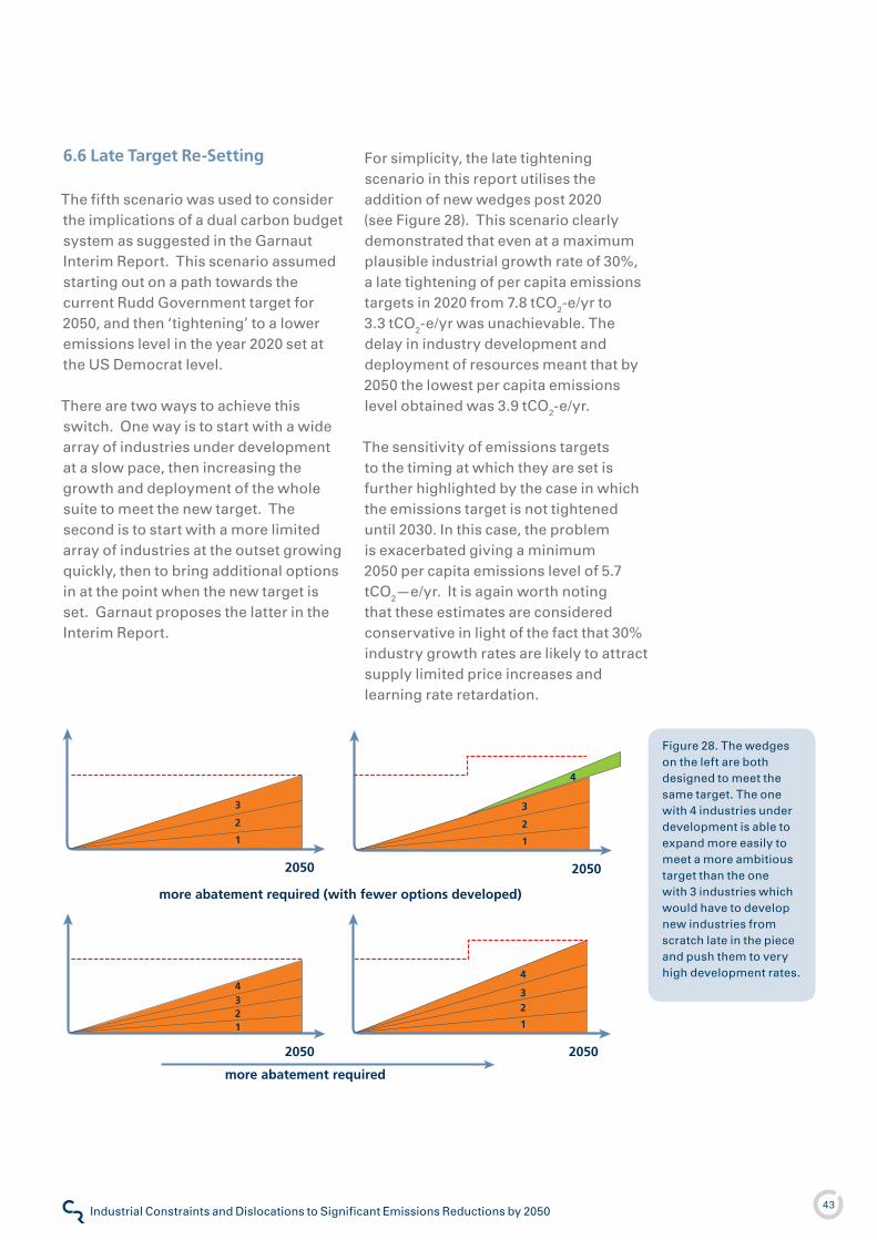
43

Climate Risk


6.6 Late Target Re-Setting

The fifth scenario was used to consider the implications of a dual carbon budget system as suggested in the Garnaut Interim Report. This scenario assumed starting out on a path towards the current Rudd Government target for 2050, and then ‘tightening’ to a lower emissions level in the year 2020 set at the US Democrat level.

There are two ways to achieve this switch. One way is to start with a wide array of industries under development at a slow pace, then increasing the growth and deployment of the whole suite to meet the new target. The second is to start with a more limited array of industries at the outset growing quickly, then to bring additional options in at the point when the new target is set. Garnaut proposes the latter in the Interim Report.

For simplicity, the late tightening scenario in this report utilises the addition of new wedges post 2020 (see Figure 28). This scenario clearly demonstrated that even at a maximum plausible industrial growth rate of 30%, a late tightening of per capita emissions targets in 2020 from 7.8 tCO2-e/yr to 3.3 tCO2-e/yr was unachievable. The delay in industry development and deployment of resources meant that by 2050 the lowest per capita emissions level obtained was 3.9 tCO2-e/yr.

The sensitivity of emissions targets to the timing at which they are set is further highlighted by the case in which the emissions target is not tightened until 2030. In this case, the problem is exacerbated giving a minimum 2050 per capita emissions level of 5.7 tCO2—e/yr. It is again worth noting that these estimates are considered conservative in light of the fact that 30% industry growth rates are likely to attract supply limited price increases and learning rate retardation.

more abatement required

more abatement required (with fewer options developed)

1

432

2050

1

3

2

2050

2050

1

4

32

1

3

2

2050

4

Figure 28. The wedges on the left are both designed to meet the same target. The one with 4 industries under development is able to expand more easily to meet a more ambitious target than the one with 3 industries which would have to develop new industries from scratch late in the piece and push them to very high development rates.

44

Climate Risk


The results show that early decisions about the emissions levels, infrastructure and the range of industries to develop, have major consequences for the ability to tighten or relax emissions levels later and the expenditure required to do so.

Achieving the lower end of the plausible emissions range requires some fundamental investments in transport alternatives and energy management infrastructure; it also requires a full suite of low emission industries to be pursued concurrently. With these industries in place and growing, it is possible to relax the speed of uptake if lower emission levels are decided upon.

The converse is not true however, if a smaller range of industries is developed, and critical transitions in the energy management and transport sectors are not made, then at some stage it may no longer be possible to deepen the trajectory and achieve the lower emissions levels within the period available, i.e. by 2050.

6.7 Irreducible Emissions

Emissions stemming from activities such as land use and some metal ore reduction (subject to CCS) may present irreducible emissions. These must be accommodated within any future carbon budget unless such activities are reduced in scale. Grazing cattle constitutes the most significant source of irreducible emissions.

If agricultural emissions are excluded from the carbon market these irreducible emissions constrain the net

carbon budget available to the other sectors and the results indicate that the upper levels are the plausible emissions range for 2050 are affected, but the lower levels (US and EU levels) cannot be achieved without these emissions being reduced.

6.8 Energy Management and Conversion Constraints

Critical advantages of fossil fuels in energy use are their ability to (a) supply energy on demand and (b) to provide high energy density, easily transported liquid fuels.

Many low emission industries are already growing rapidly in Australia or overseas. However, this growth requires augmentation of the electrical power system to manage input from new, variable and distributed supplies such as renewable energy. This will include grid-connected energy storage, which is already being used in Australia, and harnessing of significant energy storage latent in the system (Climate Risk 2007b).

Therefore simply providing an equal amount of energy is insufficient to address the needs of the power and transport sectors. Additional measures are required:

Primary energy must either be produced or stored so that it is available at the time of demand.

Energy must be converted into carriers appropriate for industrial use including chemical heat.

•

•

If a smaller range of industries is developed, and critical transitions in the energy management and transport sectors are not made, then at some stage it may no longer be possible to deepen the trajectory and achieve the lower emissions levels within the period available, i.e. by 2050.

45

Climate Risk


Energy must be converted into carriers appropriate for the needs of the transport sector.

Commercially available solutions exist for all of these tasks, and in several of these Australia is a leading innovator such as thermal energy storage and flow batteries for storing renewable energy, hydrogen production and advanced batteries for transport.

These facilitating technologies and industries will become a critical constraint if they are not able to provide the required services at a scale in keeping with the growth of the other low emission industries.

Furthermore, some of these systems will require clear choices to be made about the type of infrastructure to deploy. For example, there will be insufficient bio-hydrocarbons to meet all transport system needs in 2050 in the lower emissions scenarios. There are several options for road transport, but large scale take-up would require a choice between suitable national infrastructure such as hydrogen distribution or an electric based system.

6.9 Sequestration Infrastructure

Carbon Capture and Storage of emissions from iron, steel and cement production will be required to deliver the lower end of the plausible emission range. CCS may also be required for emissions from gas and/or coal combustion if its use is continued and the technology proves effective.

• As with energy management and conversion, the ability to achieve such capture and storage will depend on suitable infrastructure and legal frameworks being in place.

6.10 Learning Rate Retardation

As noted earlier, supply/demand mismatch is already causing prices of some low emission technologies to increase despite major increases in production volume. As a consequence, a situation in which prices fail to fall in line with production cost reductions would tend to increase costs in the short and medium term, though the major cost reductions would eventually reach the market when supply realigned with demand.

6.11 Transport Fuel Supply

Another dislocation may be the hard limit on the volume of bio-hydrocarbon resource available in Australia, even assuming that all waste hydro-carbon from agriculture can be converted to liquid or gaseous fuels.

As few alternatives exist to match the energy density of hydrocarbons, it is plausible that the aviation and shipping industries will be given primary access to the bio-hydrocarbon fuels, if and when the use of fossil fuels becomes constrained by the carbon budget.

This means that the road transport sector would need to move to a non-hydrocarbon based system, especially in the case of the deeper emissions targets. Unlike bio-fuels, this is not

46

Climate Risk


a “drop in” solution. However, the disruption involved in converting to some non-hydrocarbon based transport systems, such as electric vehicles, is rapidly being minimised as battery performance and recharging systems are improving.

The modelling indicates that adequate primary energy is available for these needs, particularly for electric vehicles, but it must be converted into suitable energy carriers. In addition to electric vehicles, many technologies are already being developed for non-hydrocarbon transport, including hydrogen for combustion or for use in fuels cells. However, hydrogen-based systems not only require a fundamental transition in vehicle and fuel production, but also in distribution infrastructure. Such a switch is highly unlikely to be market driven and may only be achievable through Government coordination. Economic and social dislocations for sectors and regions dependent on the availability of affordable transport fuels may also result in the absence of a managed transition in the transport sector.

6.12 Energy Based Community Location Changes

The geographical concentration of the existing energy industries, such as coal mining and coal power, means that an unplanned transition could see social dislocation. Equally there are requirements for rapidly growing new industries which could be constrained by lack of access to labour and expertise.

This clearly indicates opportunities to transition such communities between industries. However, such a transition needs to be orchestrated at a government level as it is unlikely to occur naturally or smoothly by market forces alone.

6.13 Major Load Location Changes

There are of course opportunities presented by communities which have skilled workers in the energy sector and requirements for expansion of new energy industries looking for skilled workers.

Figure 29 shows the location of major energy intensive metals processing facilities compared to sites of major geothermal energy resources.

6.14 Supportive Planning

Many of the abatement opportunities especially in the renewables, forestry, land-use, commercial and residential areas will be constrained or facilitated by planning mechanisms at the state, regional and local government levels. Unadjusted planning schemes may become additional transaction cost to industry development. A good example of this is the current South East Queensland Regional Plan Review. As the Regional Plan is a regulatory instrument of the state that guides and supports development in the South East Queensland area, it has the ability to support (or impede) industry development and resource exploitation. For example a planning scheme can lead to the sugar cane plantations becoming

47

Climate Risk


an industry hub for ethanol production or being paved over to form suburban housing development. It is therefore important that any alterations of the urban footprint in many areas of rapid population growth do not restrict a region’s ability to capture abatement opportunities.

6.15 Agricultural Activities

The majority of the scenarios examined require some limitation on the growth of irreducible emissions and hence specifically on agriculture which is the major contributor to such emissions. Decreases in the extent of agricultural activities run counter to the trends imposed by a growing population and increasing export demand for Australian meat and dairy products (PLCF 2006). Therefore, this particular finding indicates a significant dislocation for the agriculture industry.

By far the major source of emissions within agriculture is livestock. While dietary management has been assumed to give 20% emissions reductions

for livestock, it would appear that significant technical innovation would be required to achieve any further reductions. To obtain the necessary decrease in emissions from livestock, it may be necessary to limit the growth of Australian cattle stocks, and for the lower emissions levels possibly even reduce stock levels.

6.16 Ad Hoc Low-Carbon Policies Will Create Stranded Assets

Climate change policies based on an understated long term requirement have a high risk of inadvertently introducing inappropriate assets and technologies that may reduce near-term emissions somewhat relative to BAU, but either lock-in persistently high emissions or create stranded assets.

Appendix �2 lists currently planned new fossil fuel plants. The emissions rates of these planned new fossil plants is lower than for existing units of their fuel type, but far higher than could be feasible in meeting anticipated long-term emissions goals. This modelling

Olympic Dam

Mt Isa

Olympic Dam

Mt Isa

Bell Bay

Port Pirie

Boyne

Port Henry

Nickel West

Mine sites

Smelters

Port Hedland

Fairview

Kalgoorlie

Insolation

Highest

Lowest

Fairview

Olympic Dam

Mt Isa

Olympic Dam

Mt Isa

Bell Bay

Port Pirie

Boyne

Port Henry

Nickel West

Port Hedland

Kalgoorlie

Figure 29. It may be in Australia’s strategic interests to be a supplier of low emission energy for highly energy intensive industrial processes such aluminium production. The figures show the location of large geothermal and solar energy resources with locations of high energy demand and possible future energy demand for metals and minerals processing production.

48

Climate Risk


indicates that if the planned or proposed infrastructure is built, in some cases it may become stranded before the end of its design life or undermine national emission objectives.

Another example may be ad hoc support for biomass in the absence of strategy for how the limited stocks of bio-hydrocarbons are to be managed in the system. This could cause pursuit of technology paths which are inconsistent with the long-term fuel mix required.

6.17 Productivity and Risk

The modelling indicates that the Productivity Commission’s opinion that the Renewable Energy Target scheme operating in conjunction with an emissions trading scheme would not encourage any additional abatement but would rather impose unnecessary administration and monitoring costs2 is incorrect. Instead the results indicate that the Renewable Energy Target scheme effectively manages the risks associated with a change in national emission reduction target and the failure or underperformance of one or more low emission technologies. The modelling also indicates that the rate of industrial growth is likely to be more sustainable in circumstances where a range of low emissions industries are fostered concurrently. Thus, although the Renewable Energy Target scheme does not provide any additional abatement in the medium-term, it positions the country to achieve deeper reductions should they be required in the longer-term (as is likely, given the US and European position, to be the

case) and provides the Government’s emission reduction system with desirable resilience against the failure of one or more low emission technologies. In some respects this is an example of a wider issue in modern, open economies which, though highly efficient in the allocation of the resources, often undervalue the consequences of unusual but not unforeseeable events. The explosions of the gas plants at Varanus Island, Western Australia on 3 June 2008, which disrupted 30%-40% of Western Australia’s domestic gas supply, and at Longford, Victoria on 25 September �998, which affected 4 million people and cost industry $�,300,000,000, are two good examples of a lack of resilience to unusual but not unforeseeable events. Lack of resilience is particularly important in the case of energy, which performs a function in terms of productivity not necessarily accurately represented in national accounts, and attains even greater importance in the case of low emission technologies where the political, environmental and ultimately economic consequences of failing to achieve emission reduction targets could be severe.

2 Submission to Garnaut Climate Change Review.

49

Climate Risk


7 ReferencesABARE 2003, Excluding Technologies from the Mandatory

Renewable Energy Target, Canberra: ABARE eReport 03. 2

ABARE 2006a, Economic Impact of Climate Change Policy: The

Role of Technology and Economic Instruments, Canberra: ABARE

Research Report 06.7

ABARE 2006b, Australian Energy: National and State Projections

to 2029-30. ABARE research report number 06.26

ABARE 2007, Technology Toward a Low Emission Future, ABARE

research report number 07.�6

ABARE 2008, Energy in Australia 2008, Canberra: Department of

Resources Energy and Tourism

ABC 2007, Kangaroo farts could fight global warming, [Accessed

6th May 2008], Available from: <http://www.abc.net.au/news/

stories/2007/�2/06/2��509.htm>

Allinson, W., Nguyen, D., and Bradshaw, J. 2003, The economics

of geological storage of CO2 in Australia, APPEA Journal, Vol. 43

Bauen, A., Woods, J., and Hailes, R. 2004, Bioelectricity Vision:

Achieving �5% of Electricity from Biomass in OECD Countries by

2020, London: ICEPT and E4tech

Bloomberg 2007, U.S., Developing Nations Compromise on

Climate Talks, [Accessed ��th April 2008], Available from: <http://

www.bloomberg.com/apps/news?pid=2060�09�&sid=a70r5MZ

3qyEw>

Ceres 2005, Availability and Affordability of Insurance Under

Climate Change: A Growing Challenge for the U.S., Ceres Investor

Coalition

Chemarin, S. and Bourgeon, J-M 2007, Insurance and Adaptation

to Climate Change, Paris: Ecole Polytechnique

CIE 2006, Evaluation of Australia’s HFR Geothermal Energy

Industry, Canberra: Centre for International Economics

CIE 2007, Capitalising on the Building Sector’s Potential to Lessen

the Costs of a Broad Based GHG Emissions Cut, Canberra: Centre

for International Economics

Climate Risk 2007a. Climate Policy Analysis Tool. Australian

Labor Party �6-��-2007. Report Number CPAT – CI – ALP�6/��/2007.

Published by the Climate Institute.P/L.

Climate Risk 2007b. Towards a High-Bandwidth, Low-Carbon

Future: Telecommunications-based Opportunities to Reduce

Greenhouse Gas Emissions, Sydney: Climate Risk

CRCGA 2008, Greenhouse In Agriculture: Methane, CRC for

Greenhouse Accounting, [Accessed ��th April 2008], Available

from: <www.greenhouse.crc.org.au/greenhouse%5Fin%5Fagric

ulture/methane.cfm>

DCC 2005, National Inventory Report 2005, Canberra: Australian

Government – Department of Climate Change

DCC 2008a, National Inventory Report 2005 (Revised), Canberra:

Australian Government – Department of Climate Change

DCC 2008b, Tracking to the Kyoto Target 2007: Australia’s

Greenhouse Emissions Trends �990 to 2008–20�2 and 2020,

Canberra: Australian Government – Department of Climate

Change

DCC 2008c, National Greenhouse Accounts (NGA) Factors,

Canberra: Australian Government – Department of Climate

Change

DOE �999, Emission and Reduction of Greenhouse Gases from

Agriculture and Food Manufacturing, US Department of Energy

Office of Industrial Technologies

Eckard 2006 Are there win-win strategies for minimising

greenhouse gas emissions from agriculture? ABARE Outlook

Conference

EFF 2006, The Heat Is On – The Future of Energy In Australia,

Canberra: CSIRO

EIA 2008, Annual Energy Outlook 2008 (Revised Early Release),

Washington: Energy Information Administration

Energy Today 2008, Principal Power Stations in Australia,

[Accessed 30th April 2008], Available from: <http://www.

energytoday.com.au/contentid74.html>

EPA 2008, Inventory of U.S. Greenhouse Gas Emissions and

Sinks: �990 – 2006, Washington: U.S. Environmental Protection

Agency

European-Council 2005, Presidency Conclusions, Brussels:

European Council

European-Council �996, Communication on Community Strategy

on Climate Change, Council Conclusions, Brussels: European

Council

Gurney, A., Ford, M., Low, K., Tulloh, C., Jakeman, G. and

Gunasekera, D. 2007, Technology: Toward a Low Emissions

Future, Canberra: ABARE Research Report 07.�6

GWEC 2005, Wind Force �2, Brussels: Global Wind Energy

Council

IEA �999, Hydropower – A Key to Prosperity in the Growing World,

International Energy Agency

IEA 2000, Experience curves for energy technology policy. Paris:

OECD/IEA

IEA 2006, IEA Wind Energy Annual Report, Boulder: International

Energy Agency

IEA GIA 2007, Australian Geothermal Implementing Agreement

Annual Report – 2006, International Energy Agency Geothermal

Implementing Agreement

IPCC 2007, Climate Change 2007, Cambridge and New York:

Cambridge University Press

Mallon. K and Reardon, J. 2004, Cost Convergence of Wind Power

and Conventional Generation in Australia. Transition Institute,

June, 2004, A Report for the Australian Wind Energy Association.

Version �.34

Mallon, Karl et al. 2006. Renewable Energy Policy and Politics – A

Handbook for Decision Making. Published by Earthscan, London.

ISBN -�0: �- 84407-�26-X

McCain 2008, Climate Change, [Accessed 2nd June 2008],

Available from: <http://www.johnmccain.com/Informing/Issues/

da�5�a�c-733a-4dc�-9cd3-f9ca5caba�de.htm>

McKinsey & Company 2008, An Australian Cost Curve for

Greenhouse Gas Reduction, Sydney: McKinsey & Company

50

Climate Risk


Navaro, R. 2008, PV Prices Rising, Environmental Building News,

Vol. �7, No. 3

NREL 2003, Assessment of Parabolic Trough and Power Tower

Solar Technology Cost and Performance Forecasts, Golden:

National Renewable Energy Laboratory

Pacala, S. and Socolow, R. 2004, Stabilisation Wedges:

Solving the Climate Problem of the Next 50 Years with Current

Technologies, Science, Vol. 305

Passey, R, 2003. Driving Investment, Generating Jobs: Wind

Energy as a Powerhouse for Rural & Regional Development in

Australia March 2003. A Report for the Australian Wind Energy

Association

PLCF 2006, A Prosperous Low Carbon Future – WWF’s Proposal to

Reduce Australian Greenhouse Gas Emissions by a Third by 2030,

Sydney: WWF Australia

REN2� 2008, Renewables 2007 Global Status Report, Paris:

Renewable Energy Policy Network for the 2�st Century

Rutovitz, J. 2007, A Bright Future: 25% Renewable Energy for

Australia by 2020, Australian Conservation Foundation

Saddler, D., Diesendorf, M., Denniss, R. 2004, A Clean Energy

Future For Australia, Sydney: Energy Strategies for the Clean

Energy Future Group

The New York Times 2007, France Tells U.S. to Sign Climate Pacts

or Face Tax, [Accessed ��th April 2008], Available from: <http://

www.nytimes.com/2007/02/0�/world/europe/0�climate.html>

The New York Times 2008, The Issues: Climate Change, [Accessed

��th April 2008], Available from: <http://politics.nytimes.com/

election-guide/2008/issues/climate.html>

Taylor, M., Rubin, E., and Nemet, G. 2006, The role of

technological innovation in meeting California’s greenhouse

gas emissions targets, Berkeley: The California Climate Change

Center at UC Berkeley

UNPP 2006, World Population Prospects: The 2006 Revision,

United Nations Population Division, [Accessed ��th April 2008],

Available from: <http://esa.un.org/unpp/>

Wind Prospect 2006, Submission to the National Emissions

Trading Taskforce on the Possible Design for a Greenhouse Gas

Emissions Trading Scheme, Christies Beach: Wind Prospect

5�

Climate Risk


8 Glossary

Abatement – A reduction in greenhouse gas

emissions (also see mitigation)

ABARE - Australian Bureau of Agricultural

and Resource Economics

Adaptation -The Intergovernmental

Panel on Climate Change (IPCC) defines

adaptation as an ‘adjustment in natural or

human systems in response to actual or

expected climatic stimuli or their effects,

which moderates harm or exploits beneficial

opportunities’ (Metz et al. 200�, p.708).

AETS - Australian emissions trading scheme

Anthropogenic – The result of human

activities.

Base-load – Normally refers to a power

station that runs constantly (24 hours per

day, 7 days per week) regardless of energy

demand. Due to their slow start up and shut

down times it is more cost effective for them

to remain on.

Business as Usual – Refers to the

emissions trajectory associated with

undertaking activities without any measures

to reduce greenhouse gas emissions. Often

greenhouse gas mitigation policies are

compared to “business as usual” to show

the potential impact of the policy.

Capacity – Maximum rated power of

a power station, usually measured in

megawatts (MW).

Capacity Factor – The percentage of

yearly energy generated as a fraction of its

maximum possible rated output.

Carbon Corridor – From one year to

the next, the gap between the emissions

reductions delivered by abatement

industries, and emissions from existing

assets up until the end of their design life

is referred to as a carbon corridor. An

emissions trajectory that stays inside

this corridor will in principle achieve the

emissions reduction objectives while

avoiding stranded assets.

Carbon Credits - When pollution levels

are capped, in some schemes, it may be

possible to trade greenhouse gas pollution

rights referred to as ‘carbon credits’.

Currently, NSW has a greenhouse gas

emissions trading scheme, the Federal

Government has announced plans to

introduce a national scheme in 20�2 and

there are also voluntary abatement markets.

CO2 – Carbon dioxide, which is one of the

primary anthropogenic greenhouse gases

CO2-e - Carbon dioxide equivalent. The net

effect greenhouse gas emissions is often

presented as carbon dioxide equivalent

which is a conversion to the global warming

potential of carbon dioxide over a �00 year

period. For example, the global warming

potential for a tonne of methane is 2� times

that of a tonne of carbon dioxide.

CCS - Carbon capture and storage

Ce - Carbon equivalent

GDP - Gross domestic product

GHG - Greenhouse gas

Emissions Intensity – The emissions

generated per unit of input or output.

52

Climate Risk


Fossil Fuel – A non-renewable source

of energy formed from decayed organic

matter millions of years ago. The most

predominant fossil fuels are coal, oil and gas.

Fugitive Emissions – The emissions which

come from the mining, transportation and

storage of fossil fuels (but does not include

the emissions from fossil fuel combustion).

GDP – Gross Domestic Product – the

economic value of a country’s annual

production of goods and services.

Geosequestration – Refers to the capture

and geological (underground) storage of CO2

emissions.

Greenhouse Gas (GHG) – Gases in the

atmosphere that adsorb and emit infrared

radiation, which subsequently lead to global

warming. Most common anthropogenic

greenhouse gases are (CO2), Methane (CH4),

Ozone (O3), Nitrous Oxide (N2O) and Sulfur

Hexafluoride (SF6).

LEI - Low-emission industry

LULUCF - Land use, land use change, and

forestry.

Mitigation- The Intergovernmental Panel

on Climate Change (IPCC) defines as ‘an

anthropogenic intervention to reduce the

sources or enhance the sinks of greenhouse

gases’ (Metz et al. 200�, p. 7�6).

MRET - Mandatory Renewable Energy

Target

Mt- Mega-tonnes. One mega tonne is one

million tonnes. Greenhouse gas emissions

are often displayed in mega-tonnes carbon

dioxide equivalent per annum (MtCO2-e/yr)

(see MtCO2-e).

MtCO2-e - Mega-tonnes carbon dioxide

equivalent (MtCO2-e) is the internationally

recognised measure used to compare the

emissions from the various greenhouse

gases. This measures factors in differences

in global warming potential and converts

them to a carbon-dioxide equivalent. For

example, the global warming potential for a

tonne of methane over �00 years is 2� times

that of a tonne of carbon dioxide.

Mtoe - one million tonnes of oil equivalent

NEM – The National Electricity Market. The

NEM is a wholesale market for electricity

supply which delivers electricity to market

customers in all states and territories, except

for Western Australia and the Northern

Territory, through the interconnected

transmissions and distribution network.

NEMCO - The National Electricity Market

Management Company Limited administers

the National Energy Market (see NEM).

Peaking Plant – Normally refers to power

stations which run at peak times to meet

short term peaks in electricity demand.

Photovoltaic Cell – A renewable energy

technology which converts sunlight into

electrical energy.

Power - Energy transferred per unit of

time. Electrical power is usually measured

in watts (W), kilowatts (kW) and megawatts

(MW). An appliance drawing �000 Watts (�

kW) for � hour is said to have used � kilowatt

hour (� kWh) of electricity.

53

Climate Risk


ppm - Parts per million

PV - Photovoltaic (solar power)

Renewable Energy - Energy which comes

from natural processes and which are

replenished in human time frames or cannot

be exhausted (sources of renewable energy

include wind, biomass, solar radiation,

geothermal energy, wave and tidal power).

TWh/yr - Terawatt hours per year. A

terawatt is one million, million (�0�2) watts

Wind Farms – A collection of wind turbines

which connect to common substations to

feed into the main electrical grid.

Wind Turbine – A renewable energy

technology that converts air currents into

mechanical energy which is then used to

generate electrical energy.

With Measures – Describes an emissions

trajectory with greenhouse gas mitigation

measures and generally shows the deviation

from the business-as-usual projection.

54

Climate Risk


9.1 Scenario Settings

9.1.1 Emissions Levels

The scenarios considered are based on a plausible set of future emissions levels for 2050, given existing national commitments and international positions.

9.1.2 Population

In order to consider the effects of population dynamics, this model includes population as a variable. The Australia Bureau of Statistics’ 2006 projections estimate that Australia will have a population of between 23 million and 3� million by 2050. The ABARE baseline is based on a median population estimate of 28 million in 2050 and this is used for all scenarios presented here. However, it is important to recognise that population policy will have an effect on emissions trajectories and climate policies.

9.1.3 Climate Change Impacts

Ironically, most modelling for climate change mitigation activity neglects the effect of climate change impacts and adaptation. For example, there is already strong evidence that increasing numbers of climate-related natural catastrophes (such as severe hurricanes) are having a discernable impact on insured losses (Cheramin & Bourgeon 2007, Ceres 2005).

Projections for increased losses and the costs required to adapt the physical infrastructure will have a material

effect on global and national GDP. This dynamic has been included in our analysis via a coefficient to adjust GDP such that it reflects the burden of costs associated with climate change impacts and adaptation. Estimates for degree of impact on the economy are available in the research conducted by Dr Roger Jones, CSIRO as published by the Energy Futures Forum (EFF 2006).

A 3% climate change impact retardation of GDP by 2050 is used across all the presented scenarios.

9.1.4 Consumption

The ABARE baseline contains implicit assumptions which express increased wealth as increased physical consumption of energy and other commodities (Gurney 2007). However, if we are to consider doubling in the GDP of an already-wealthy country, it is plausible that additional wealth may be realised through activities not necessarily directly coupled with consumption. For example, increased wealth could be expressed as increased leisure time, voluntary work or community activity with less added consumption. A decoupling factor is included in the model to reflect a fraction of wealth that may not result in increased commodity consumption.

For the scenarios in this particular report, the de-coupling factor is set to zero, i.e. increased wealth is assumed to be fully coupled to increased consumption.

If we are to consider doubling in the GDP of an already-wealthy country, it is plausible that additional wealth may be realised through activities not necessarily directly coupled with consumption. For example, increased wealth could be expressed as increased leisure time, voluntary work or community activity with less added consumption.

9 Appendix: Scenario Settings and Outputs

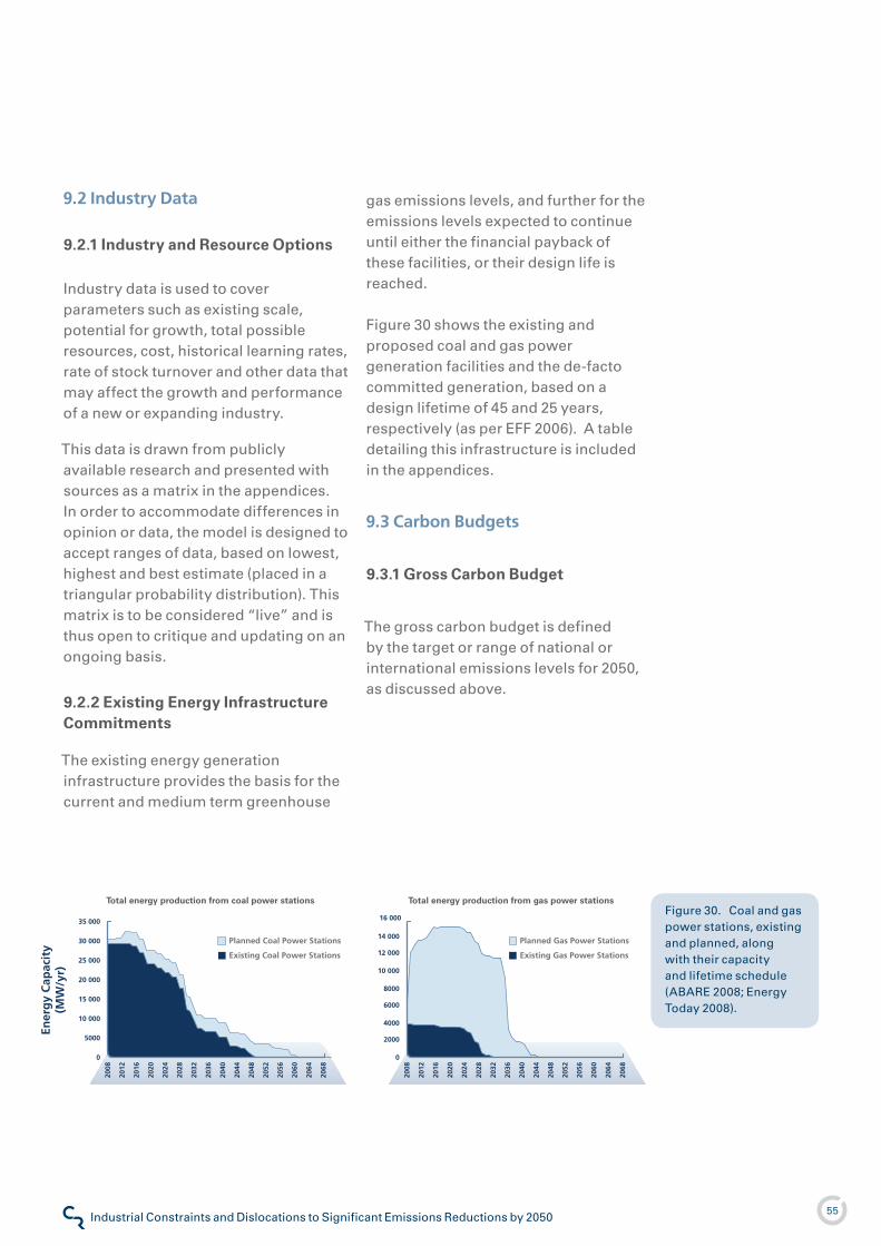
55

Climate Risk


9.2 Industry Data

9.2.1 Industry and Resource Options

Industry data is used to cover parameters such as existing scale, potential for growth, total possible resources, cost, historical learning rates, rate of stock turnover and other data that may affect the growth and performance of a new or expanding industry.

This data is drawn from publicly available research and presented with sources as a matrix in the appendices. In order to accommodate differences in opinion or data, the model is designed to accept ranges of data, based on lowest, highest and best estimate (placed in a triangular probability distribution). This matrix is to be considered “live” and is thus open to critique and updating on an ongoing basis.

9.2.2 Existing Energy Infrastructure Commitments

The existing energy generation infrastructure provides the basis for the current and medium term greenhouse

gas emissions levels, and further for the emissions levels expected to continue until either the financial payback of these facilities, or their design life is reached.

Figure 30 shows the existing and proposed coal and gas power generation facilities and the de-facto committed generation, based on a design lifetime of 45 and 25 years, respectively (as per EFF 2006). A table detailing this infrastructure is included in the appendices.

9.3 Carbon Budgets

9.3.1 Gross Carbon Budget

The gross carbon budget is defined by the target or range of national or international emissions levels for 2050, as discussed above.

2008

Year

15 000

10 000

35 000

25 000

30 000

20 000

Ener

gy

Cap

acit

y(M

W/y

r)

Existing Coal Power Stations

Planned Coal Power Stations

2068

2064

2060

2056

2052

2048

2044

2040

2036

2032

2028

2024

2020

2016

2012

5000

0

2008

Year

6000

4000

14 000

10 000

12 000

8000

2068

2064

2060

2056

2052

2048

2044

2040

2036

2032

2028

2024

2020

2016

2012

2000

0

16 000

Existing Gas Power Stations

Planned Gas Power Stations

Total energy production from coal power stations Total energy production from gas power stationsFigure 30. Coal and gas power stations, existing and planned, along with their capacity and lifetime schedule (ABARE 2008; Energy Today 2008).

56

Climate Risk


9.3.2 Net Carbon Budget

The net carbon budget is what remains after irreducible emissions (see below) are subtracted from the gross carbon budget(s).

The net carbon budget is then allocated between industries which still have ongoing greenhouse gas emissions such as those that use carbon capture and storage (CCS) which still has a component of lost gases, as well as continuing/residual greenhouse gas emissions from conventional emission sources such as aviation. The fixed nature of the carbon budget means that if one or more low emissions industries develop weakly or fail altogether, then the available carbon budget is reduced.

The Model is capable of distributing the net carbon budget in any proportion between various industries. For the scenarios considered in this report, the 2050 net carbon budget is assumed to be split equally between CCS energy generation and transport fuels.

9.3.3 Irreducible Emissions

There are some activities for which no immediate solutions exist to eliminate their current emissions. For example, there is little prospect at present that emissions from livestock will be reduced to zero. Likewise, pyrometallurgical techniques used in the production of metals such as iron will inherently produce greenhouse gas emissions as long as society uses steel, cement, ceramics and ammonia production (though some of these may be captured by CCS).

While emissions in these areas can be minimised, the literature indicates there is an irreducible level of emissions that cannot be further mitigated using known technology unless the activity itself is reduced (though such reductions are possible, this analysis avoids such an assumption wherever possible). Put another way, we do not assume that the nation eats or exports less meat or that it produces less steel in order to address emissions related to climate change. However, some of the more challenging emissions reduction targets examined in this report cannot be achieved without assuming some reduction in certain activities. When such an assumption is required, it is detailed in the description of the scenario. Otherwise, the composition of the economy and sectors is assumed to remain unchanged, or to be as specified by ABARE.

Stationary Energy and Transport: Almost all stationary energy emissions are assumed to be reducible in the model, subject to available industry development time and implementation of power management and storage infrastructure. Similarly, all transport energy emissions are assumed to be reducible in the model, subject to cost, available time and implementation of non-fossil energy carrier modes and infrastructure.

Industry: It is assumed that most emissions from industrial applications can be reduced. However, there are some industrial processes for which there are

a)

b)

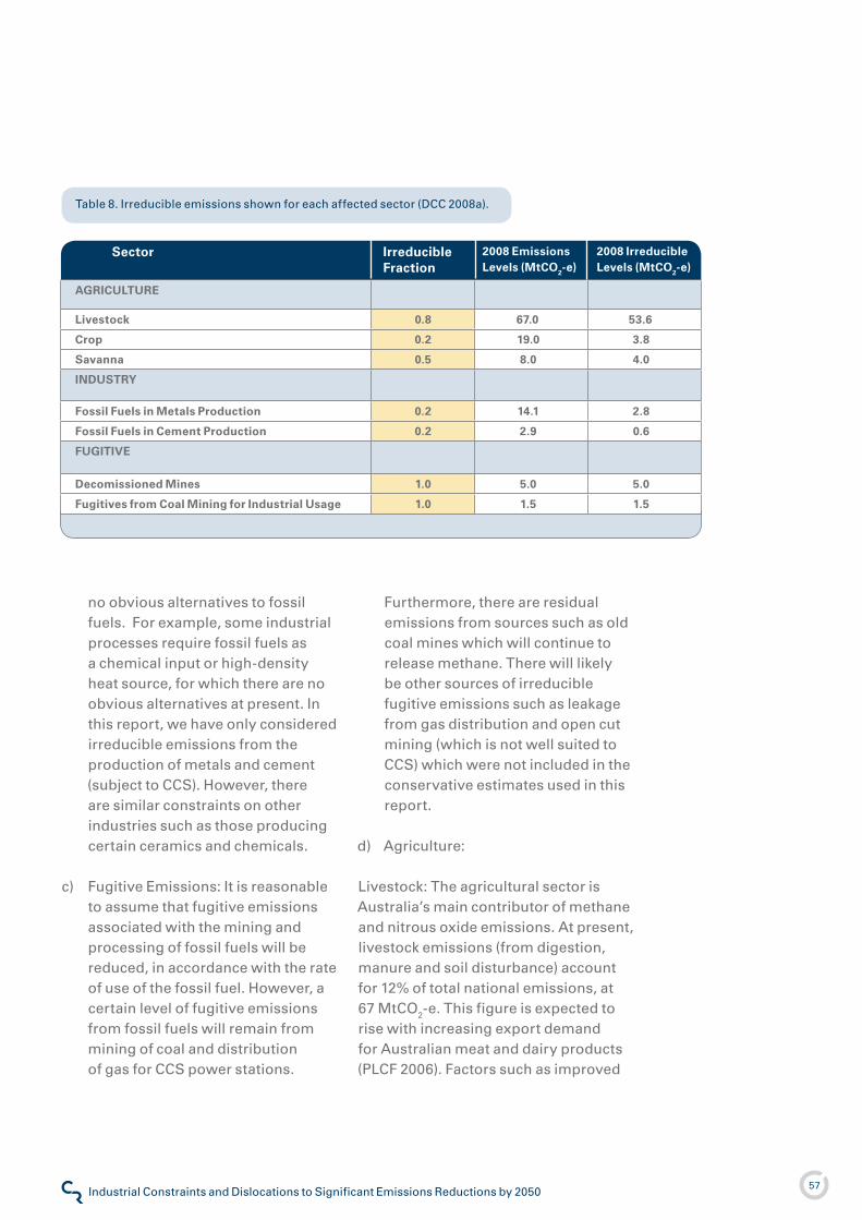
57

Climate Risk


no obvious alternatives to fossil fuels. For example, some industrial processes require fossil fuels as a chemical input or high-density heat source, for which there are no obvious alternatives at present. In this report, we have only considered irreducible emissions from the production of metals and cement (subject to CCS). However, there are similar constraints on other industries such as those producing certain ceramics and chemicals.

Fugitive Emissions: It is reasonable to assume that fugitive emissions associated with the mining and processing of fossil fuels will be reduced, in accordance with the rate of use of the fossil fuel. However, a certain level of fugitive emissions from fossil fuels will remain from mining of coal and distribution of gas for CCS power stations.

c)

Furthermore, there are residual emissions from sources such as old coal mines which will continue to release methane. There will likely be other sources of irreducible fugitive emissions such as leakage from gas distribution and open cut mining (which is not well suited to CCS) which were not included in the conservative estimates used in this report.

Agriculture:

Livestock: The agricultural sector is Australia’s main contributor of methane and nitrous oxide emissions. At present, livestock emissions (from digestion, manure and soil disturbance) account for �2% of total national emissions, at 67 MtCO2-e. This figure is expected to rise with increasing export demand for Australian meat and dairy products (PLCF 2006). Factors such as improved

d)

AGRICULTURE

Livestock 0.8 67.0 53.6

Crop 0.2 19.0 3.8

Savanna 0.5 8.0 4.0

INDUSTRY

Fossil Fuels in Metals Production 0.2 14.1 2.8

Fossil Fuels in Cement Production 0.2 2.9 0.6

FUGITIVE

Decomissioned Mines 1.0 5.0 5.0

Fugitives from Coal Mining for Industrial Usage 1.0 1.5 1.5

Sector Irreducible Fraction

2008 Emissions Levels (MtCO2-e)

2008 Irreducible Levels (MtCO2-e)

Table 8. Irreducible emissions shown for each affected sector (DCC 2008a).

58

Climate Risk


animal selection, pasture feed and waste management practices may reduce these livestock emissions. Early indications from the Cooperative Research Centre for Greenhouse Accounting suggest it may be possible to reduce methane emissions from dairy cows by up to 20% (CRCGA 2008), leaving 80% as irreducible emissions.

Crops and Savanna: Crop production in Australia accounts for greenhouse gas emissions of about �9 MtCO2-e/yr, arising from inefficient fertiliser application, soil disturbance and residue burning. Recent research has shown that up to 80% of fertiliser-related emissions could be eliminated with minimal loss of pasture growth. This could be done through improved fertilisers, crop demand matching and soil and animal management (Eckard 2006). Similarly, emissions from soil disturbance and residue burning could be greatly reduced with less-intrusive tilling practices which retain crop residue (DOE �999). Based on these assumptions, the maximum crop-related emissions abatement has been limited to 80% in this analysis. Irreducible emissions from savanna have been estimated at 50% of current levels.

LULUCF: All land use, land use change and forestry (LULUCF) greenhouse gas emissions are assumed to be reducible in the model.

Waste: All emissions from waste are assumed to be reducible in the model.

e)

f)

9.4 Baseline Resource Requirements

9.4.1 Energy

The ABARE 2007 baseline is used as a basis for the BAU projections of energy demand and emissions, with some important modifications applied to adjust for population, climate change impacts and consumption (PCCC).

It should be noted that the ABARE reference case has some questionable trends, for example, future energy demand for transport. In 2004 transport consumed 28 Mtoe (million tonnes of oil equivalent) of final energy in Australia; taking into account current levels of mobility in goods and efficiency, and for a population increasing from 20 to 28 million, energy consumption for transport would be expected to be about 40 Mtoe. However, ABARE projections for transport final energy demand are 60 Mtoe. Given normal advances in vehicle and systems efficiency, this figure might be expected to be somewhat lower.

9.4.2 Non-Energy

The ABARE 2007 baseline is also used by the presented scenarios as the baseline for non-energy activity and emissions, including agriculture, land use, land-use change and forestry, waste, fugitive emissions and industrial emissions not related to energy consumption.

59

Climate Risk


9.5 Policy Framework

9.5.1 Implementation Timing

Much of the policy and industrial development covered in the model must occur over limited timeframes, but will nonetheless generate major transitions. As a result, the Model outcomes are very sensitive to the point at which policies are implemented and industrial development commences. This may range from policies which are already in place (for example, commercial energy efficiency), policies which are imminent (such as the 20% Mandatory Renewable Energy Target [MRET]) and policies or technologies which may not leverage commercial deployment for some time (e.g. CCS).

9.5.2 Market Dynamics

Industry development is very sensitive to the type of policy being used. For example, the EU feed-in tariffs for low-emissions technologies seek to develop many different renewable energy industries simultaneously, with suitable adjustments to ensure their respective costs are not development constraints.

In contrast, technology-neutral policy tools such as the AETS and MRET work by making emission abatement industries compete with each other on a price basis. This tends to produce a quasi-sequential industry development process, with the least costly measures being adopted first.

Another issue is the long- versus short-term nature of policy frameworks.

Long-term/stable mechanisms tend to create supply driven markets, in which industries can gauge demand well in advance and make suitable investment in production. Short-term mechanisms do not support long-range investment in the private sector, and in their case supply tends to follow demand; these mechanisms have been characterised by persistent supply shortages and higher prices. These higher prices tend to manifest themselves as reductions to the production learning rates (i.e. costs fall slowly or stop falling).

9.5.3 Learning Rates

Learning rates are a measure of the cost reduction for a doubling of production (Taylor 2006). The change in unit cost with increasing cumulative production of a given technology is depicted in an experience curve, the slope of which is related to the learning rate. See Figure 3� and Figure 32 for several important emission abatement technologies.

It can be seen that, in general, the early stages of a given technology’s market adoption will see it “learn more” from market experience. That is, “the same absolute increase in cumulative production will have more dramatic effect at the beginning of a technology’s deployment than it will later on” (IEA 2000).

It can be argued that Australia as a small market can afford to take a back seat on technology development and be a late implementer. However, many parts of industry growth are inescapably local, including the development of expertise

Technology-neutral policy tools such as the AETS and MRET work by making emission abatement industries compete with each other on a price basis. This tends to produce a quasi-sequential industry development process, with the least costly measures being adopted first.

60

Climate Risk


Cumulative electricity production (TWh)

1000

Cost of electricity (ECU(1990/kWh)

0.01

0.01

0.10

0.10

1.00

1.00

10.00

10.00

Photovoltaics (~65%)

1985

19951980

1995

Wind power - average (82%) Electricity from biomass (~85%)

Supercritical coal (~97%)

Wind power - best performance (82%)

NGCC (96%)

100

Cumulative Capacity Installed (MW)

101 1 000 000100 00010 0001000100

Capital Cost 2004 $/W

0.01

0.10

1.00

10.00

100.00

PV

STE

SWH

SCR(coal)

windFGD

SCR(gas)+

+ ++

+++

+ + + ++++++ +

Figure 3�. Experience curves for emissions abatement technologies showing the capital cost for increasing cumulative installed capacity around the world from the �970s until the early 2000s (Taylor 2006).

Figure 32. Experience curves showing the cost of electricity for increasing cumulative production of various technologies installed in the European Union �980-�995 (IEA 2000).

6�

Climate Risk


and private sector capacity including planning, legal contracting, component manufacture or assembly, and key trades such as electrical installation and site works.

This analysis takes a neutral view as to where in the world technology and industry are developed. It is therefore assumed that Australia, as well as participating in the process of per capita emissions convergence, is also sharing in the industrial development of the major solution technologies and their industries. It is of course possible that Australia may focus particular attention on specific technologies within this mix that may be less likely to receive support by the broader international community, including solar hot water, deep geothermal energy and metals processing efficiency.

9.5.4 Learning Retardation

For most emissions abatement solutions the price of the technology decreases as the production volume increases (i.e. a positive learning rate; Taylor 2006, IEA 2000). However, in some cases, there can be a zero reduction in price or even an increase in prices with increased production (i.e. a negative learning rate). This scenario has recently become a serious concern for wind energy and photovoltaic (PV) energy (Wind Prospect 2006, Navaro 2008). In the case of solar water heating, the increase in the unit cost with increased production is thought to be related to increases in materials and labour costs that were not overcome by the modest technical improvements over the same period (Taylor 2006).

From the �970s to the early 2000s, wind energy and photovoltaic energy both exhibited positive learning rates. More recently, however, both these technologies have suffered price increases due to supply shortages. According to an Australian wind industry developer, “Wind power has actually increased in cost by up to 20% in the last 24 months due to unprecedented world-wide demand and a subsequent component supply shortage” (Wind Prospect 2006). Similarly, photovoltaics have experienced manufacturing and materials constraints consistent with supply shortage. Figure 33 illustrates the resultant rise in photovoltaic module price as production has increased.

9.5.5 Price Volatility Risk Loading

The model does not include risk loading for fossil fuel supply which, though not as acute in Australia as in markets such as the EU and USA, still affects the global price of energy. This is an important effect that the authors hope to introduce when further refinements are incorporated in the model.

9.6 Scenario Outputs

The scenario outputs for emissions and energy are available as probability distributions. For simplicity, the outputs are summarised as means and cumulative results, to provide a succinct overview of the findings. Other important outputs include the rates of industry growth required to achieve the emissions range and the effect of when industry growth is commenced. These issues are presented in detail in the findings section of this report.

62

Climate Risk


Cumulative production (MW)

1 100 00010 000100010010

1

10

100

Module price (2006$/W)

1980

2006

Historical prices

1990: Prices rise due to limited supply of silicon wafers

1996: Moderate demand growth (16%) with manufacturing overcapacity results in declining prices

2001: Manufacturing capacity catches up with demand resulting in lower prices

2004 - present: Strong demand coupled with silicon supply shortage leading to price increases

Figure 33. Persistent silicon shortages and high demand are causing prices of PV modules to rise in recent years even as production has increased (Navaro 2008).

3.49

3.73

3.25

3.61

3.01

3.37

3.13

20

15

10

5

0

25

30

4.21

4.09

3.97

3.85

Range of returned values for a given parameter

Nu

mb

er o

f d

iscr

ete

mo

del

ru

ns

wh

ich

retu

rned

th

e as

soci

ated

val

ue

Figure 34. Example distribution for an output for a sample run of the model, presented as a histogram and percentile distribution. These indicate the range of possible outcomes, the most likely outcomes and a probability distribution for any given output.

63

Climate Risk


11 Appendix: Matrix of Key Model Inputs

Existing Large Hydro 26.4 TWh/yr 0.2 - 0.3

Small Hydro 3.8 - �0.� TWh/yr 0.5 - 0.7

Wind Power 200 TWh/yr 0.25 - 0.35

Geothermal 58 TWh/yr 0.8 - 0.9

Solar Power Stations 270 TWh/yr 0.25 - 0.73

Sea and Ocean Energy � - 50 TWh/yr 0.2 - 0.45

Building Integrated PV �9� TWh/yr 0.� - 0.2

Domestic Solar Thermal 382 TWh/yr 0.�

Bio-Hydrocarbons 92 TWh/yr

Fossil Fuels with CCS 0.4 - �.� tCO2-e/MWh

(captured)

0.5 - 0.7

Low Emission Technology Maximum Resource by 2050 Capacity Factor

It should be noted that the estimates of renewable energy resource are conservative. For example, the constraints applied to the resource available to geothermal energy, solar power stations and sea and ocean energy for 2050 may have actually been removed by that time, in which case the available resource could be significantly larger.

Avoided Aviation 30 - 50%

Aviation/Shipping Efficiency �0 - 20%

Reduced use of Vehicles �5 - 50%

Efficient Vehicles 20 - 50%

Efficient Buildings 28 - 72%

Metals Energy Efficiency 35 - 50%

Industrial Energy Efficiency 20 - 50%

Agriculture 30 - 50 MtCO2-e

LULUCF 22 - 37 MtCO2-e

Forestry 0 - 20 MtCO2-e

Waste 0 - 2�.5 MtCO2-e

Fugitive 25.� MtCO2-e

Sector Emissions Abatement

Sources: EFF 2006, Saddler 2004, IEA GIA 2007, CIE 2006, ABARE 2006, DCC 2008, GWEC 2005, NREL 2003, Rutovitz 2006, PLCF 2006, Bauen 2004, Allinson 2003, IPCC 2007, ABARE 2003, Taylor 2006, IEA 2000

Sources: EFF 2006, Saddler 2004, ABARE 2006, DCC 2008, PLCF 2006

Table 9. Key model inputs for various technologies.

Table �0. Key model inputs for various sectors.

64

Climate Risk


12 Appendix: Table of Existing and Proposed Fossil Fuel Power Plants

Coal Power Station State Year Commissioned Capaci t y (MW)

Currently Installed

Loy Yang A Vic �984/87 2�20Hazelwood Vic �964/7� �600Bayswater NSW �982/84 2640Yallourn W Vic �973/75/8�/82 �480Eraring NSW �982/84 2640Stanwell Qld �993/96 �400Gladstone Qld �976/82 �680Loy Yang B Vic �993/96 �000Tarong Qld �984/86 �400Mt Piper NSW �992/93 �320Liddell NSW �97�/73 2000Vales Point NSW �978 �320Muja WA �965/8�/85/86 �040Callide B Qld �988/89 700Northern SA �985 530Wallerawang C NSW �976/80 �000Callide C Qld 200� 900Swanbank A & B Qld �966/69/70/73 908Collie WA �999 330Kwinana A & C WA �970/76 880Munmorah NSW �969 600Millmerran Qld 2002 852Tarong North Qld 2002 443Redbank NSW 200� �50Morwell Vic �958/59/62 �95Anglesea Vic �969 �60Collinsville Qld �998 �88Thomas Playford B SA �960 240

Coal Power Station State Year Commissioned Capacity (MW)

Planned InstallationsEraring Upgrade NSW 20�� 360Mt Piper Upgrade NSW 2008 �80Mt Piper Extension NSW 20�3 �500Tornago Stage 3 NSW not known 270Loy Yang A upgrade Vic 2009 ��0Kogan Creek Qld 2008 750Macarthur Coal Qld not known 200Bluewaters stage � WA 2008 208Bluewaters stage 2 WA 20�0 208Bluewaters stage 3 WA 20�2 208Midwest WA 20�� 400

Table ��. Currently installed coal-fired power stations.

Table �2. Planned coal-fired power stations.

Sources: ABARE 2008, Energy Today 2008


65

Climate Risk


Gas Power Stations State Year Commissioned Capacity (MW)

Currently InstalledTorrens Island SA �967/77 �280

Pelican Point SA 2000 478

Kwinana B WA �970 240

Smithfield NSW �997 �60

Newport Vic �980 5�0

Jeeralang A and B Vic �979/80 449

Valley Power Vic 2002 300

Somerton Vic 2002 �50

Bairnsdale Vic 200� 92

Swanbank E Qld 2002 385

Oakey Qld 2000 288

Yabulu Qld 2005 240

Mica Creek Qld �997/200� �58

Mica Creek Qld �998 �32

Mica Creek Qld �997 35

Roma Qld �999 80

Barcaldine Qld �996 57

Osborne Qld �998 �85

Hallet SA 2002 �83

Dry Creek SA �973 �56

Quarantine SA 2002 92

Mintaro SA �984 90

Ladbroke Grove SA 2000 84

Kwinana WPC WA �972 2�

Cockburn WA 2003 240

Worsley WPC WA 2000 �20

Mungarra WA �990-9� ��2

Kalgoorlie WA �984-90 62

Tiwest WA �999 36

Geraldton WA �973 2�

Bell Bay Tas �97� 240

Table �3. Currently installed gas-fired power stations.


66

Climate Risk


Gas Power Stations State Year Commissioned Capacity (MW)

Planned InstallationsBamarang stage � NSW 2009 400Bamarang stage 2 NSW 20�0 300Bega NSW 2008 ��5Buronga NSW not known �20Cobar NSW 2009 ��5Herons Creek NSW not known �20Marulan stage � NSW 20�0 320Marulan stage 2 NSW 20�� 450Munmorah NSW 2009 660Parkes NSW not known �20Tallawarra NSW 2008 400Tomago NSW 2008 360Uranquinty NSW 2009 640Wellington NSW 2009 640Mortlake Vic 2009 �000Morwell HRL plant Vic 2009 400Chinchilla Qld 2009 242Condamine Qld 2009 �35Fairview Qld 20�5 �00Moranbah/Nebo Stage � Qld 2008 420Moranbah/Nebo Stage 2 Qld 20�3 270Moranbah/Nebo Stage 3 Qld 20�7 2�0Spring Gully Qld 2009 �000Stanwell Qld 2008 300Townsville Qld 20�0 400Arckaringa CTL Project SA 20�4 560Hallett expansion SA not known 250Pelican Point expansion SA 2008 300Centauri � WA 2008 �68Kwinana WA 2008 320Neerabup WA 2009 330Tamar Tas 2009 200

Table �4. Planned gas-fired power stations.


67

Climate Risk


Other Fossil Fuelled Power Stations State Year Commissioned

Capacity (MW)

Currently Installed

Mt Stuart Qld �998 304

Mackay Qld �976 34

Snuggery SA �978-97 63

Port Lincoln SA �998-00 50

Angaston SA 2005 40

Kwinana WPC WA �970/76 880

Pinjar WA �990-92, �996 586

Currie Tas �952 20

Whitemark Tas �984/94 6

Planned Installations

Wagerup Alinta Stage 2 WA 2009 �76

Table �5. All other currently installed and planned fossil fuel power stations.


68

Climate Risk


Limitations in manufacturing capacity, resource development, labour and skills generally restrict the stable expansion of new industries. While exceptions may exist in the short-term, consistent annual growth rates higher than 30% generally result in supply dislocations that cause temporary increases in prices. This leads to retardation in the expected learning rates of these industries as increases in production volumes do not achieve the previously obtained reduction in price. Even if the price increases caused by supply shortage could be tolerated, industrial limitations in the materials, labour and skills required to expand production mean that growth rates higher than 30% are physically unsustainable over the long-term.

The three industries operating at average annual growth rates greater than 25% in Figure 35 have all recently experienced supply limited price increases and hence learning rate

retardations (Wind Prospect 2006, Navaro 2008). This phenomenon is manifested via component shortages within the wind and photovoltaic industries and demand related increases in the cost of grain and oil feedstock for biodiesel. Where the ultimate resource can be expanded (this may not be the case for biodiesel feedstock which competes with food), short-term supply dislocations will generally be corrected over time and commensurate price reductions achieved. However, while excessively high industry growth rates are maintained, this process of equilibration will continue to be hampered.

706050

Biomass power

Solar PV, grid-connected

Biodiesel (annual production)

Biomass heating

Geothermal power

Large hydropower

Small hydropower

Ethanol (annual production)

Solar hot water/heating

Solar PV, off-grid

Geothermal heating

Wind power

0 40302010

Percent

Figure 35. Average annual growth rates of renewable energy capacity from 2002 to 2006. (REN2� 2008)

13 Appendix: Sustainable Industry Growth Rates

69

Climate Risk


Climate Risk Pty Limited (Australia)

Sydney: +6� 2 8006 �320 Brisbane: +6� 7 3368 2902

www.climaterisk.net

Climate Risk Europe Limited London: + 44 20 8�44 45�0

Manchester: + 44 �6 �273 2474 Climate Risk

Documents

Report Emissions Reductions by 2050 Dislocations to Significant … · 2008-08-18 · Climate Risk Industrial Constraints and Dislocations to Significant Emissions Reductions by 2050