SR-430-2604 1

FINAL REPORT

COMPARISON OF IUIODELS FOR PREDICTING LANDFfLt METHANE RECOVERY

Prepared for:

THE SOLID WASTE ASSOCIATION OF NORTH AMERICA 1100 Wayne Avenue

Suite 700 Silver Spring, Maryland 209 1 0

Prepared By:

SCS ENGINEERS 11 260 Roger Bacon Drive Reston, Virginia 22090

(703) 471-61 50

In Association With:

Mr. Oonsld Augenstein Institute for Environmental Management

4277 Pomona Avenue Palo Alto, California 94306

(41 5) 856-2850

March 1997 File No. 0295028

This publication was reproduced from the best available copy Submitted by the subcontractor and received no editorial review at NREL

NOTICE

This report was prepared as an account of work sponsored by an agency of the United States government. Neither the United States government nor any agency thereof, nor any of their employees, makes any warranty, express or implied, or assumes any legal liability or responsibility for the accuracy, completeness, or usefulness of any information, apparatus, product, or process disclosed, or represents that its use would not infringe privately owned rights. Reference herein to any specific commercial product, process, or service by trade name, trademark, manufacturer, or otherwise does not necessarily constitute or imply its endorsement, recommendation, or favoring by the United States government or any agency thereof. The views and opinions of authors expressed herein do not necessarily state or reflect those of the United States government or any agency thereof.

Printed on paper containing at least 50% wastepaper, including 20% postconsumer waste

ACKNOW LEDG MEWS

Development of this report was sponsored by the National Renewable Energy Laboratory (NREL). The work was managed by Ms. Charlotte Frola and Ms. Dianne De Roze of the Solid Waste Association of North America (SWANA). Authors for this report were Mr. W. Gregory Vogt of SCS Engineers and Mr. Don Augenstein of the Institute for Environmental Management (I EM) . We thank Ms. Stacey Derners of the Northeast Maryfand Waste Disposal Authority (NMWDA) for her contributions specific to landfill gas model comparisons and optimization procedures. We are grateful to the companies and landfill owners/operators wbo provided the landfill site data necessary to conduct this project. We also wish to acknowledge the hetpful suggestions and guidance of the peer review staff assembled by SWANA for preparation of this report.

The Peer Review Team included:

Dr. Jean Bogner a Mr. H. Lanier Hickman, P.E.

Mr. Stephen G. Lippy, RE., D.E.E. Mr. Ray Huitric

Mr. John Pacey, P.E. MI. Alex Roqueta Mr. Carlton Wiles

In particular, we thank Mr. Ray Huitric of the Sanitation Districts of Cos Angeles County for his numerous contributions, diligent efforts, and superior work products which have served to advance the field’ of landfill methane modeling.

These advisors participated as individuals, not as official representatives of their organizations or institutions. We are grateful for their assistance and their insights; however, SWANA was solely responsible for the overall conduct of the study.

EXECUTIVE SUMMARY

Landfill methane models are tools used to project methane generation over time from a mass of landfilled waste. These models are used for sizing landfill gas (LFG) coflection systems, evaluations and projections of LFG energy uses, and regulatory purposes. Compared to other alternatives (such as installation of a full-scale LFG recovery system or the use of test wells and the performance of a pumptest program), modeis have advantages in terms of low cost and relatively rapid results.

Improvement of landfill methane models has been a priority for the LFG industry. The literature is not replete with models that have been compared or calibrated with-landfill methane field data and modeling of methane generation and recovery is not sufficiently advanced. Current landfill methane models are uncertain. However, as more LFG collection systems we installed (for regulatory and other reasons) and operated within lined landfills, better landfill data will become available for modeling. As a result, modet uncertainties probably can be reduced.

The objective of this project was to select various landfill methane models and to provide a comparison of model outputs to actual long-term gas recovery data from a number of well managed and suitable landfills. Another objective was to use these data to develop better estimates of confidence limits that can be assigned to mode1 projections.

This project assessed trial model forms against field data from available landfills where methane extraction was maximized, waste filling history was well-documented, and other pertinent site information was of superior quality. Date were obtained from 18 U.S. landfills. Four landfill methane models were compared: a zero-order, a simple first order, a modified first order, and a multi-phase first order model. Models were adjusted for "best fit" to field data to yield parameter cornbinations based on the minimized residual errors between predicted and experienced methane recovery. The models were optimized in this way using two data treatments: absolute value of the differences (arithmetic error minimization) and absolute value of the natural log of the ratios (logarithmic error minimization).

Application of the two data treatments yielded parameter combinations which were model dependent and similar to those used in the LFG industry. Values for Lo, the methane yield potential, were consistent for the three first-order models under the arithmetic error optimization function, ranging from 2,300 to 2,200 cubic feet of methane per ton of landfilled waste. Under the logarithmic function, at least one parameter combination for each of the four models resulted in an Lo within the 2,000 to 2,200 cubic feet of methane range. Values for k, the first order decay rate constant, were more varied and model dependent. Under the arithmetic optimization , k values ranged from 0.05 t o 0.08 per year; under the logarithmic optimization, k values rsnged from 0.03 to 0.06 per year.

Minimization of logarithmic error gave better results than those demonstrated by arithmetic error minimization in the form of a nakow, more specific band of parameter combinations for best fit optimization.

Regression coefficients (r2) were calculated to compare modeled versus actual methane recovery. Results for ? ranged from 0.928 to 0.937 for the arithmetically optimized models; for the models optimized logarithmically, the r' values ranged from 0.914 to 0.955, indicative of reasonable correlations. Similarity of the regression coefficient results indicates that the four models were similar in predictive ability.

The four landfilt methane models also were compared through examination of data distributions of the numerical ratios of the measured methane recovery values to the modeled recovery over the spectrum of data points established for the study landfills. Plots were developed to show 10 and 90 percent probability limits around median values based on minimization of arithmetic and logarithmic errors.

Generally, the set of study landfills showed rather wide probabiIity limits, meaning the models could project methane recovery within a factor of about 1.5 for 80 percent of the landfill data points. The spread or dispersion was greater for the remaining data points. Furthermore, the probability limits for the models optimized via logarithmic minimization were narrower than those established with the arithmetic optimization.

A simple computer program was developed for each of the four study models which accepts keyboard inputs for model parameters in order project methane generation over time. For one model form the program provides probability limits (upper and lower bounds) based on the minimization of arithmetic error procedures described in the report.

CONTENTS

1 INTRODUCTION ............................................ 1-1 Landfill Methane Models ....................................... 1-1 Previous Modeling Studies ..................................... 1-2 Project Objectives ........................................... 1 4 Report Organization and Content ................................. 1-5

2 SELECTION OF STUDY LANDFILLS AND METHANE MODELS ....... i .... 2-1 Background ................................................ 2-1 Selection of Study Landfills ..................................... 2-3 Selection of Landfill Methane Models .............................. 2-5

3 APPROACH FOR MODEL OPTIMIZATION AND COMPARISON ............ 3-3 Overview of Approach ........................................ 3-1 Model Optimization Procedure ................................... 3-2 Illustration of Trial Model Optimization ............................. 3-3

4 RESULTS ................................................. 4-1 Parameter Combinations Derived From Minimized Error ................. 4-1 Model Comparisons .......................................... 4-2

5 COMPUTER PROGRAM FOR LANDFILL METHANE MODELS .............. 5-1

6

7

RECOMMENDATIONS FOR FURTHER WORK m . - 0 0 611

REFERENCES.. ............................................. 7-1

APPENDICES

A Project Landfill Site Data B Ptoject Questionnaire C Methane Gas Recovery Program

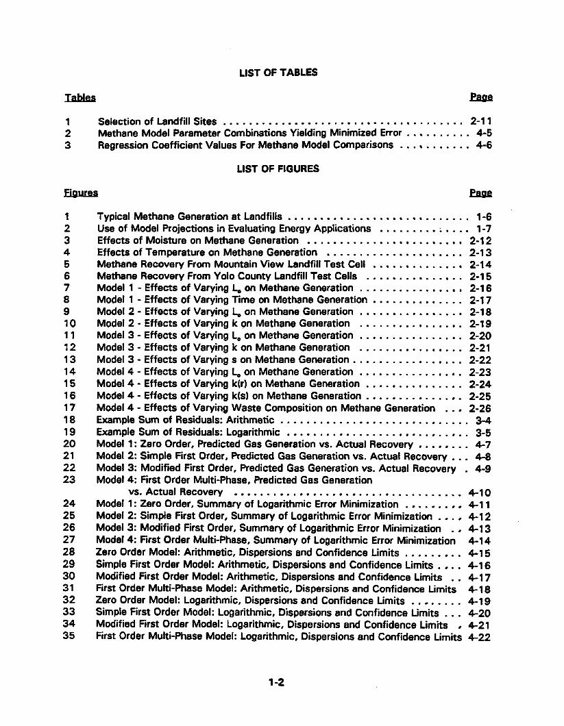
LIST OF TABLES

TaMes Paae 1 2 3

Selection of Landfill Sites . . . . . . . . . . . - . . . . . . . . . . . . I . . . 2-1 1 Methane Model Parameter Combinations Yielding Minimized Error . . . . . . . . 4-5 Regression Coefficient Values For Methane Model Comparisons . . . . . . . . . . 4-6

LIST OF FIGURES

Fiaures Pacle 1 2 3 4 5 6 7 8 9 10 11 12 13 14 15 16 17 18 19 20 21 22 23

24 25 26 27 28 29 30 31 32 33 34 35

Typical Methane Generation at Landfills . . . . . . . . . . . . . . . . . 1-6 Use of Model Projections in Evaluating Energy Applications . . I . . . . ; . . 1-7 Effects of Moisture on Methane Generation - . . . . . . . . . . . . 2-12 Effects of Temperature on Methane Generation . I . . . . . . . . I . . . 2-13 Methane Recovery From Mountain View Landfill Test Cell . . . . . . 2-14 Methane Recovery From Yolo County Landfill Test Cells . - . . . . . . . . . 2-1 5 Model 1 - Effects of Varying L, on Methane Generation . - . . . . . . . - . . 2-16 Model 1 - Effects of Varying Time on Methane Generation . . . . I . . . 2-1 7 Model 2 - Effects of Varying L,, on Methane Generation # . . . . . I . . 2-18 Model 2 - Effects of Varying k on Methane Generation . . . . . . . . . 2-19 Model 3 - Effects of Varying L, on Methane Generation . . . . . . . . . . . . . 2-20 Model 3 - Effects of Varying k on Methane Generation . . . . . . . . . I . 2-21 Mode1 3 - Effects of Varying s on Methane Generation . . . . . . . . I . 2-22 Model 4 - Effects of Varying L, on Methane Generation . . . . . . . - . . . . 2-23 Model 4 - Effects of Varying k(r) on Methane Generation . # . . . . . . . . . 2-24 Model 4 - Effects of Varying k(s) on Methane Generation - . . . . . . . . . 2-25 Model 4 - Effects of Varying Waste Composition on Methane Generation . - 2-26 Example Sum of Residuals: Arithmetic . . . . . . I - . . . . . . . . . . . . . . 3-4 Example Sum of Residuals: Logarithmic . . . . . . I . . . . . . . . . . 3-5 Model 1: Zero Order, Predicted Gas Generation vs. Actual Recovery . . 4-7 Model 2: Simple First Order, Predicted Gas Generation vs. Actual Recovery . . - 4-8 Model 3: Modified First Order, Predicted Gas Generation vs. Actual Recovery . 4-9 Model 4: First Order Multi-Phase, Predicted Gas Generation

vs. Actual Recovery . . . . . . . I . . . . - . . . . . . . .. 4-10 Model 1: Zero Order, Summary of Logarithmic Error Minimization . . . . . 4-1 1 Model 2: Simple First Order, Summary of Logarithmic Error Minimization . . 4-12 Mode1 3: Modified First Order, Summary of Logarithmic Error Minimization 4-13 Model 4: First Order Mufti-Phase, Summary of Logarithmic Error Minimization 4-1 4 Zero Order Model: Arithmetic, Dispersions and Confidence Limits . . . . . . . 4-1 5 Simple First Order Model: Arithmetic, Dispersions and Confidence Limits . . . 4-16 Modified First Order Model: Arithmetic, Dispersions and Confidence Limits . . 4-1 7 First Order Multi-Phase Model: Arithmetic, Dispersions and Confidence Limits 4- 1 8 Zero Order Model: Logarithmic, Dispersions and Confidence Limits . . . I . . 4-19 Simple First Order Model: Logarithmic, Dispersions and Confidence Limits . . . 4-20 Modified First Order Model: logarithmic, Dispersions and Confidence Limits 4-21 First Order Multi-Phase Model: Logarithmic, Dispersions and Confidence Limits 4-22

1-2

SECTION 1

INTRODUCTION

LANDFILL METHANE MODELS

A landfill methane model is a tool used to project methane generation over time from a mass of waste. In its simplest form, a model predicts methane generation or recovery from a single batch of waste, landfilled at a single given point in time. Total methane generation or recovery from a tandfill (or a portion of the waste mass) is then the sum of outputs from all batches in the landfill. Typically, the unit for the parameter time is 8 year.

Typic81 components of models may include an interval before methane generation starts (lag time) and subsequent intervals of rising, constant, and falling production, depending on the model. A simplified example of a model profile from a single waste batch is illustrated in Figure 1 8 showing a 1-year lag time and estimated methane generation over 8 45-year period. Although Figure 1 shows a single line for simpIicity, model projections are inherently probabilistic", and confidence limits should be assigned to their projections.

Landfill gas (LFG) models are used for:

a c-on svstems. LFG collection and treatment equipment must be installed at most larger landfills in response to regulatory requirements under the Clean Air Act. In addition, landfill sites often require such systems for purposes of subsurface migration control, odor control, and other reasons. Modeling can be an effective tool to appropriately size the wellfield and associated LFG collection, treatment, and/or recovery equipment.

0 . ns of wfill With knowledge of equipment and operating costs, unit energy revenues, and other key factors, "probabilistic" model projections can be used to estimate the LFG or methane yields of landfills, size equipment, estimate costs, and evaluate the spectrum of likely investment returns.

0 w t o r v DUTDOSBS. Model projections have been used to calculate landfill emissions and to support establishment of LFG and methan8 emission requirements.

Figure 2 shows steps in a hypothetical model application for an energy project. The top illustration shows three curves for a hypothetical model which projects likelihood that gas recovery will exceed given values at a landfill site. The lowest curve is a recovery value which might be exceeded 90 percent of the time; the middle curve is the median (where gas recovery might be exceeded 50 percent of the time) and the top curve is the recovery that would be attained 10 percent of the time.

The middle illustration of Figure 2 represents equipment performance for two different capacities (or gas usage rates) compared to a gas recovery projection at the 50 percent

1-1

level. Similarly, the bottom illustration represents the same set of equipment capacities compared to more conservative gas recovery estimates (Leo, methane recovery that would be realized or exceeded 90 percent of the time).

Solid waste industry investments and expenses associated with LFG control and recovery are significant. For example, the capital cost of equipment to produce 1,000 Mwe of electricity from LFG would exceed $1 billion (EPRt, 1992; EPA, 1993). Both EPA (1993) and EPRl (1 992) estimate LFG electric potential at 5000 + MWe, given adequate electricity sale prices. Furthermore, given the implementation of current Clean Air Act requirements, the costs for LFG controls are expected to rise in the future.

Theoretically, as landfill methane models are refined and improved, their use should reduce errors in sizing of energy and recovery equipment, yield improved cost-benefit calculations, and reduce project risks. Such models would provide significant added value annually to the LFG industry and the public.

Compared to other alternatives, models have advantages in terms of low cost and relatively rapid results. To estimate a landfill's methane generation, one alternative to models (short of installing a full-scale recovery system) is the use of test wells and the performance of a pump-test program. However, costs for pump tests can exceed $100,000 and require three months or more to accomplish; the tests have inherent imprecisions; and the field resutts represent points in time for the test location(s) in the landfill rather than long-term projections for the entire landfill. A goal for landfill methane models is to provide information of comparable accuracy to extrapolations of pump test results for the entire landfill.

Although models have the potential to provide these benefits, advantages of models can be realized only to the extent models are sufficiently developed. Modeling of landfill methane generation and recovery is not sufficiently advanced.

PREVIOUS MODELING STUDIES

Model development for prediction of gas recovery and other purposes began with the increase in sanitary landfilling in the 1970's. The first "modeling" consisted of the application of "rules of thumb", and such estimates (albeit refined) continue to be used in the LFG industry (Walsh, 1994) . Qualitative descriptions of the LFG generation process 8lSO were developed by Farquhar and Rovers in 1973. Other investigators attempted more rational bases for prediction of LFG or methane on the basis of available but Iimited landfill data (Alpern, 1973; Ham, 1979; and Ham, et. af., 1979). Around the same time, more quantitative model predictions were first attempted in the Los Angeles basin in the U. S.

Numerous variables affect waste decomposition in landfills and the subsequent production of methane. The "standard" analytical models, such as the Manod, that predict performance of microbial processes under defined temperature, nutrient, and other biological conditions, cannot be applied effectively to landfills. Researchers have found it difficult to obtain field data from a unique batch of waste to compare with a model's predicted methane generation curve. In part, this difficutty occurs because methane recovery from landfills typically is aggregated output from many years of waste placement, rather than from individual batches of waste within the landfill.

1-2

Model development mostly has been empirical; it has consisted of the application or the testing of a wide range of postulated generation curves (i.e., variations on the curve of Figure 1). Forms of such curves have been assumed on various bases inchding mechanistic assumptions about decomposition (Van Zanten and Scheepers, 1 995; Zison, 1990; Augenstein and Pacey, 1 99 1 1.

The literature is not replete with landfill methane models that have been compared or calibrated with field data. The following summarizes some of the published and unpublished work

Good data are becoming available from landfib operated in Southern California by the Sanitation Districts of Los Angeles. These landfills have accurate waste placement, composition, methane recovery, and other relevant data, and are yielding promising model forms to predict methane recovery.

0

Several proprietary models exist and are applied by engineering firms and others. However, the development details largely are unknown and little published information is available which compares the proprietary models' predictions with field experience.

Oonk, et. al. (1 994) examined methane recovery from landfills in Holland. This work correlated four trial models with a moderate amount of data from 12 landfilts and showed good "fit" of postulated models with site data. However, methane generation data were short term- three years, maximum.

Peer, et. al. (1992) for the U. S. EPA examined methane recovery from a set of 21 US. landfills. One recuvery rate was measured at a single "point in time" (the study year) for each landfill. Peer, et. al. found recovery to be correlated with waste in place, by what was termed an "emission factor": i.e., methane recoverable per unit of waste per unit of time, determined for each individual study landfill. Correlations were not made with waste age (i.e., time since filling) or other variables such as rainfall or temperature. For the study landfills, the emission factor ranged from 2.5 to 6.5 cubic meters of methane per minute per million metric tons of waste in place.

Augenstein and Pacey (1 991 ) showed comparisons of two landfills' data to B proprietary model which suggest conformance of gas generationlrecovery to first order kinetics. This paper also presented data from Zison (1990) wherein a similar model gave reasonable results (recovery ranging from -30 to + 50 percent of predicted) for three of four Southern Cafifornia landfills.

Current landfill methane models are uncertain. These uncertainties are due to several factors, including:

1 -3

Sparseness and quality of the data used for modet development and Cali bration;

Limited time frames for the available field data used;

0 Inappropriate application of available data:

Varying geographic/ciimatic conditions; and

Other factors specific to the landfill design and operations such as landfill depth, liners, and leachate recirculation.

As more LFG collection systems are installed and operated within lined landfills, better landfill data likely will become available for modeling. As a result, model uncertainties probably can be reduced.

Given the present status of landfill methane models and the utifity of such models to landfill operators, LFG-to-energy developers, and regulators, the National Renewable Energy Laboratory (NREL) funded this project through 8 contract with the Solid Waste Association of North America (SWANA). SWANA subsequently retained SCS Engineers and the Institute for Environmental Management to perform this study and prepare this report.

PROJECT OBJECTIVES

The purpose of this project was to select various landfill methane models and to provide a comparison of model outputs to actual gas recovery data from a number of well managed and suitabIe landfills. Specific objectives included:

Identify US. landfills with available operational and gas recovery data suitable for model comparisons and obtain data from them;

Select trial model forms to test against landfill data;

0 Use landfill data to adjust model parameters and assess the reasonableness of the trial models;

0 Identify confidence limits which can be assigned to models;

Assess the effect of site variables on methane generation and recovery;

0 Make available the study's findings in the form of an easy-to-use computer proQram; and

Make recommendations for future study.

1 4

Comparison of landfill methane models involves a number of corpplex issues and choices as to procedures to be used. This report provides detail on the background and reasoning as to why certain approaches were taken and discusses advantages and limitations of the findings with respect to methane model users in the LFG industry.

REPORT ORGANlZATlON AND CONTENT

The remaining sections of the report are organized as follows:

a Section 2 presents background on landfill methane generation and the selection of landfill methane models for further evaluation;

Section 3 discusses the approach used for comparison of model outputs to actual gas recovery data;

Section 4 presents results of the model comparisons and derivations for parameter values of the optimized models. It also presents error and confidence limits based on data from the study landfills;

Section 5 discusses the computer program developed for users t o create outputs from the four models evaluated;

Section 6 presents recommendations for further study, based on the findings and analytical results; and

Section 7 lists htersture references noted in the report.

Supplemental information is appended as referenced herein.

1 -5

SECTION 2

SELECTION OF STUDY LANDFILLS AND METHANE MODELS

This section reviews LFG generation as it relates to predictive modeling. Variables and uncertainties inherent in both the development of models and their application are discussed, as well as the criteria used in to select this study's landfills for model development. Finally, this section discusses the basis for the landfill methane models selected for further examination.

BACKOROUND

The approach for this study was to compare selected landfill methane models (model curves) with gas recovery field data from several landfills so as to yield the best predictions, or "best fits". An underlying assumption to this approach is that there is an "average" curve that can best represent and predict methane generation and/or recovery, and that curvefitting procedures can identify one or more "best" models closest to this average curve. This approach has been applied in previous studies (Oonk, 1994; Zison, 1991 ; and Augenstein and Pacey, 199 1 ).

Certain terms are used in this report specific to LFG models. Models may refer to either total gas (i.e., LFG) or methane. Because methane is normally the component of interest, this report refers to landfill methane (unless otherwise specified). The term generation refers to the methane generated within the waste mass. Recovery refers to the methane recovered from the waste mass because it is a parameter that can be measured. (This avoids the ambiguous term "production" which can to refer to either methane generation or the actual fraction of methane recovered from that generated).

Landfill gas is the mixture of carbon dioxide and methane, and other trace components, generated from waste by bacterial decomposition of waste organics. For cellulose, the principal source of gas from tandfilled waste, the conversion reaction is:

(CdH,OO1)n + n H,O - > 3nCH, + 3n COP cellulose monomer bacteria

Discussions of landfilled waste decomposition are found in a number of references, including Halvadakis, et. al. (1 9831, 8arlaz (1 9901, Ham and co-workers (several papers), Pohland and co-workers (several papers), and Augenstein 8nd Pacey (1 99 1 ).

Several factors govern waste decomposition. Moisture level commonly is considered of greatest importance. Another factor, well-established on fundamental grounds and from laboratory tests (but largely neglected in modeling), is temperature. Figures 3 and 4 show the pronounced effects of moisture and temperature, respectively, from work of Halvadskis, et. a!. (1 983) snd Ashate, et. al. (1 9931, respectively.

Other factors also affect the rate and quantity of methane generation from wastes. These can include waste composition, waste nutrient level, and the presence or absence of

24

buffering agents (which may be provided from such sources as cover soils). Landfill operational factors, such as air intrusion, landfill covers, waste compaction, and leachate recirculation also can impact methane generation. Because factors tend to vary from landfill to landfill, some degree of modeling uncertainty is a given.

Factors giving rise to uncertainties in methane models include:

0 Variation in generation due to factors mentioned above;

0 Measurement inaccuracies or errors;

Recovery efficiency variables;

Substantial variation of relevant parameters spatially within the landfill, becoming more significant with increasing moisture and temperature in certain 'pockets' or zones; and

0 Discrepancies between the model form chosen and the "true" underlying average generation within a given dataset used to estimate model parameters.

For example, recovery efficiency is a source of variability. It likely varies with the landfill geometry; liner and cover materials (e.g., clay or membrane); cover maintenance; design, installation, and maintenance of the LFG extraction system; and other factors. Recovery efficiency can change with time during active landfilling, with lower recovery expected in the first few years, higher recoveries expected after closure, and levels somewhere in between during the interim years.

Landfill-to-landfill variations in methane generation and recovery occur for reasons that are evident. For example, precipitationfinfiltration through cover soils may be greater into some landfills than others, and subsequent methane generation may be accelerated where there is more infiltration. However, excessive oxygen infiltration into the waste mass impedes methane production. Also, warm region landfills decompose more rapidly than cold region landfills. While landfills self-warm as methane generation occurs, heat dissipation rates vary.

What is important for modeling is not so much the source of uncertainties but their effect in the aggregate. In aggregate the uncertainties create deviations between any model's prediction and subsequent field experience. This deviation is referred to as "model error" or "uncertainty" in this report. The degree of model error intrinsic to a given model is important to describe, but has not been explicitly characterized for any large database in landfill methane model work to date. There exist "probabilistic" ways of expressing probability of methane recovery lying within any given set of bounds. Identification and expression of these bounds were project objectives.

2-2

Some uncertainties can be reduced. One way is to select landfills with superior data. Uncertainties also can be compensated for or reduced by establishing correlations between site factors and gas recovery.

The value of reliable methane recovery data and corresponding reliable site factors was illustrated by Oonk, et. al. (1 994). Using data from 12 Dutch landfills with good apparent recovery and good knowledge of site history and site factors (e.g. annual waste placement, design, extraction monitoring, etc.), three different trial models "fitn recovery with similar accuracy (by statistical indices). Maximum error of about 30 percent was reported, generally better than reported by U.S. experience'.

SELECTION OF STUDY tANOFILLS

Candidate landfills for this study ("study landfills") were sought with the following characteristics:

Gas recovery efficiency is maximized. This was considered associated with as many as possible of the following features:

- Scavenging of LFG for energy-limited equipment;

- Well-maintained covers (clay or synthetic) and frequent well monitoring;

- Good well density;

- *Efficient" well configuration in terms of close spacing, greater (rather than lesser) depth;

- Wellhead and header pipeline methane contents at 40 to 50 percent (rather than 50 to 60 percent), suggesting tuning of wells for maximum recovery;

- Maintenance of methane below regulatory limits by surface scan (now mandated in many regions of the country); and

- Maintenance of odors below odor thresholds.

Accurate waste gate receipt and placement history.

Such 'goodness of fit" may relate to the relative uniformity of Dutch landfills and wastes, but nonetheless supports use of the best site data.

2-3

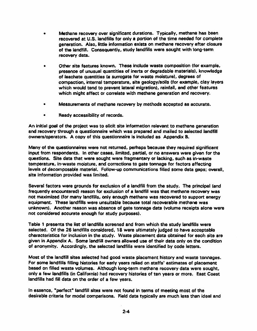
Methane recovery over significant durations. Typically, metbane has been recovered at US. landfills for only 8 portion of the time needed for complete generation. Also, little information exists on methane recovery after closure of the IandfilL Consequently, study landfills were sought with long-term recovery data.

Other site features known. These include waste composition (for example, presence of unusual quantities of inerts or degradable materials), knowledge of leachate quantities (a surrogate for waste moisture], degrees of compaction, internal temperature, site geology/soils (for example, clay layers which would tend to prevent lateral migration), rainfall, and other features which might affect or correlate with methane generation and recovery.

Measurements of methane recovery by methods accepted as accurate.

Ready accessibility of records.

An initial god of the project was to elicit site information relevant to methane generation and recovery through a questionnaire which was prepared and mailed to selected landfill ownerdoperators. A copy of this questionnaire is included as Appendix B.

Many of the questionnaires were not returned, perhaps because they required significant input from respondents. In other cases, limited, paatial, or no answers were given for the questions. Site data that were sought were fragmentary or lacking, such as in-waste temperature, in-waste moisture, and corrections to gate tonnage for factors affecting levels of decomposable material. Follow-up communications filled some data gaps; overall, site information provided was limited.

Several factors were grounds for exclusion of a landfill from the study. The principal (and frequently encountered) reason for exclusion of a landfill was that methane recovery was not maximized (for many landfills, only enough methane was recovered to support energy equipment. These landfills were unsuitable because total recoverable methane was unknown). Another reason was absence of gate tonnage data (volume receipts alone were not considered accurate enough for study purposes).

Table 1 presents the l i s t of landfills screened and from which the study landfills were selected. Of the 26 landfills considered, 18 were ultimately judged to have acceptable characteristics for inclusion in the study. Waste placement data obtained for each site are given in Appendix A. Some landfill owners allowed use of their data only on the condition of anonymity. Accordingly, the selected landfills were identified by code letters.

Most of the landfill sites selected had good waste placement history and waste tonnages. Far some landfills filling histories for early years relied on staffs' estimates of placement based on filled waste volumes. Although long-term methane recovery data were sought, only a few landfills (in California) had recovery histories of ten years or more. East Coast landfills had fill data on the order of a few years.

In essence, "perfect" landfill sites were not found in terms of meeting most of the desirable criteria for model comparisons. Field data typically are much less than ideal and

often are incomplete. Generally, the best data were obtained from the landfill sites operated by the Sanitation Districts of Los Angeles.

Because this study represents a limited set of landfills, data from landfills not typical of the study landfills may not be comparable. However, efforts were made to include a cross- section of U.S. landfills (with the normal uncertainties and methane recovery variations) so as to allow basic comparisons in model outputs (including predictive ability and confidence iimits) to "average" or "typical" U.S. landfills. Models limited to this predictive ability still represent a significant advance over previous published work.

SELECTION OF LANDFILL METHANE MODELS

Landfill methane models considered for the study were based on previous studies and usage in the LFG industry. Some models were not selected for inclusion (examples are certain model forms proposed in Zson [1990]). Kinetic estimates (which have significant "guess" components, precedent, and field experience) are important model forms in the industry. Model forms that are commonly considered are discussed in Van Zanten and Scheepers (1 995) and in Augenstein and Pacey (1 99 1).

A goal of the project was to select landfill methane models with fairJy simple structures and are easy to use. In part, this is because any model of sufficient complexity-with sufficient adjustable parsmeters-can be fit to any dataset. Yet, ability to obtain a perfect fit does not confirm a model's correctness.

Certain field measurements should (in principle) provide ideal methane generation profiles upon which to base model forms. For example, an ideal measurement for purposes of model development wouid be of long-term methane generation/recovery for a landfill cell filled over a short interval, with known relevant parameters (such as moisture content, etc.). The cell could be monitored closely over time so that total methane output could be assumed to represent a batch methane generation profile and thus, provide a "true" model curve for landfilled wastes under a given set of conditions.

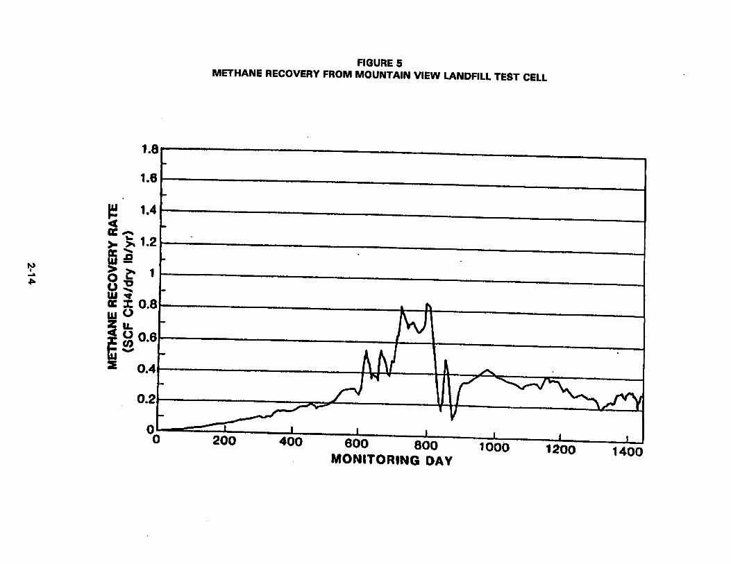
There have been some measurements of methane generation from single batches along these lines. The results are informative, but less than helpful with respect to ideals of modelers. In one case a completely enclosed control cell was operated as part of a landfill test project (Augenstein and Pacey, 1991 1. The generation curve from this enclosed cell is shown in Figure 5.

In another case, gas recovery data were collected from five waste cells at a California landfill (Yolo Central) over a six-year interval. These data yield normalized methane per year per ton of waste in place for each of the five cells as a function of time since waste placement. These results are depicted in Figure 6.

Both Figures 5 and 6 should represent a close match of an ideal batch generation profile (i.e., the "model curve") for the particular waste masses measured. However, the generation and/or recovery field data are irregular over time, with many short-term

2-5

variations that are difficult to explain. In essence, field data typically do not match mathematical model curves in the published literature.

As landfilling proceeds over a tonger time and more waste is added which contributes to the landfill's generation/recovery profile, short-term fluctuations in generation from individual waste lots average out. Even if a postulated model form does not match the generation profile of 8 single waste batch exactly, term generation profiles of "real" landfills.

c8n be useful to replicate the longer

With these issues in mind, four model forms (taking the form of mathematical expressions) were selected for evaluation and comparison. The background and basis for each model choice are discussed briefly below.

With each model, parameters which can be adjusted to optimize the model are shown in boxes beneath the model equations. Each model requires input values for adjusted waste placement data and the noted parameters to make projections for a given model year. Because the model equations for the value G (methane generation by volume) are for individual "batches" or years, the batches must be summed for the years desired to provide the gas generation time curve. Mathematical expressions for the models are as follows: .

Where:

G = methane generation, million cubic feet per year; W = waste in place, tons; L, = methane yield potential, cubic feet methane per ton of waste; t = time, years; t, = lag time (between placement and start of generation); and t, = time to endpoint of generation.

Parameters adjustable to fit field data for optimization: t, and & (or the interval &-I$.

This model is used fairly extensively in the landfill as industry.

2-6

Fim Or- -k (t-t,) G = W L , k e

Where:

G = methane generation, million cubic feet per year; W = waste in place, tons; L, = methane yield potential, cubic feet methane per ton of waste;; t = time after waste placement, years; t, = lag time (between placement and start of generation); and k = first order rate constant.

I Pararoeters to vary initially for best fit to field data: k aad t I Variants of this model are used extensively. A public domain computer version is available from €PA.

Where:

G = methane generation, million cubic feet per year; W = wiste in place, tons; L, = methane yield potential, cubic feet methane per ton of waste: t = time after waste placement, years; t, = lag time (between placement and start of generation); k = first order decay rate constant; and s = first order rise phase rate constant.

I Parameters to adjust to fit field data: t,, k, and s.

This model is described by Van Zanten and Scheepers (1995). The model form assumes that methane generation/recovery initially may be low (i.e., there is a "lag"). Recovery then rises to a peak before declining in what is essentially exponential fashion.

2-7

Where:

G = methane generation, million cubic feet per year; W = waste in place, tons; L,, = methane yield potential, cubic feet methane per ton of waste; t = time after waste placement, years; t, = lag time (between placement and start of generation); k,r, = first order decay rate constant for rapidly decomposabla waste; k,, = first order decay constant for slowiy decomposable waste; F,, = fraction of rapidly decomposable waste; and F,, = fraction of slowly decomposable waste.

(Parameters to adjust to fit field data: t,, k(r),k(s), FIr) , and F(s). I Model 4 is a refinement of Model 3 (the modified first order model) 8bOve. Its assumptions are the same, except that differing waste fractions are assumed to decompose at different rates. Variants of this model are applied comrnercialIy. This model gave the best results (by narrow margin) in modeling work of Oonk, et. al. (1994).

To estimate annual methane emissions, each model accepts inputs for the refuse filling history and methane generation parameters. Some input parameters are used by several models; others are specific to one particular model. To illustrate model outputs and the effects of varying parameters, trial runs of the four models were used to estimate methane emissions from an example landfill. Parameter sensitivity was ascertained by varying one parameter with selected values while keeping other parameters constant.

The example landfill for this parameter sensitivity effort received 100,000 tons of refuse per year for 10 years (i.e., resultant waste-in-place is 1 million tons).

Mbdel-

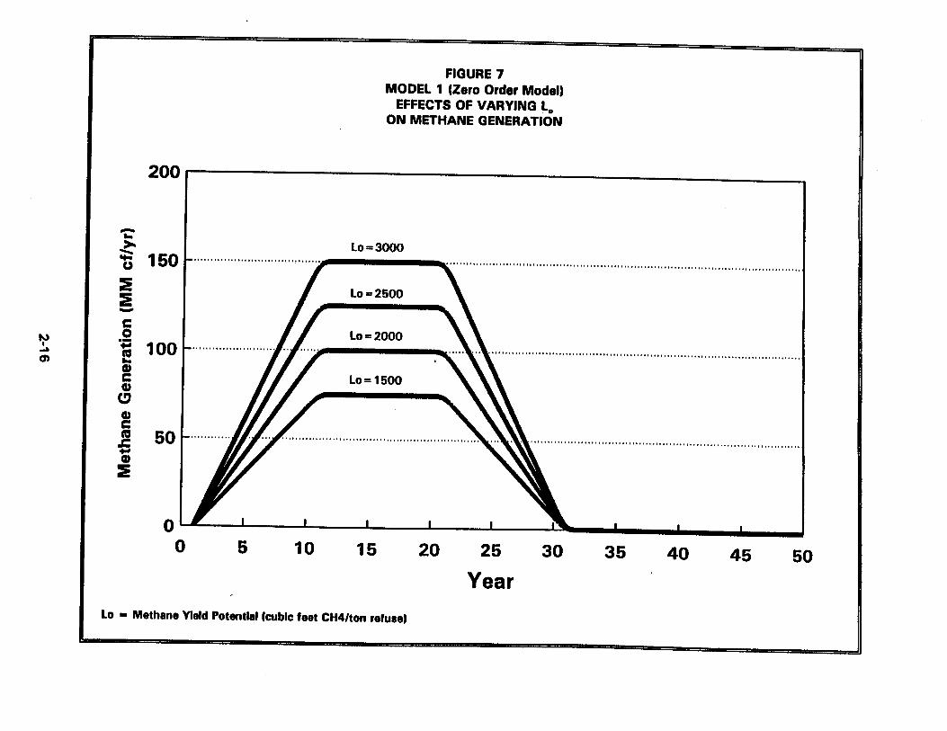
The Zero Order Model has two parameters: the methane yield potential (Lo) and duration of methane generation (time in years). A graphic summary of the sensitivity for these two parameters is shown in Figure 7 (for Lo) and Figure 8 (for time).

As shown in Figure 7, the impact of varying Lo in Model 1 is direct: during peak methane generation periods (i.e., the flat peak of the curve), cubic feet of methane per year vary inversely with Lo.

2-8

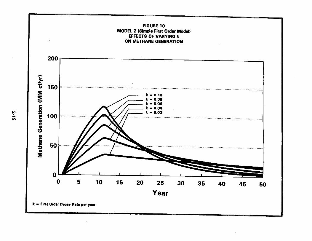
The Simpiified First Order Model has two parameters: the methane yield potential (Lo) and the decay rate (k). Figures 9 and I 0 show sensitivity to the parameters Lo and k.

As shown in Figure 9, the impact of varying Lu in Model 2 is significant: the estimated rate has a direct relationship to the selected value for Lo. Similarly, Figure 10 shows that as k is increased, recovery increases and time span decreases. The rate of falloff for methane generation increases markedly with increasing k.

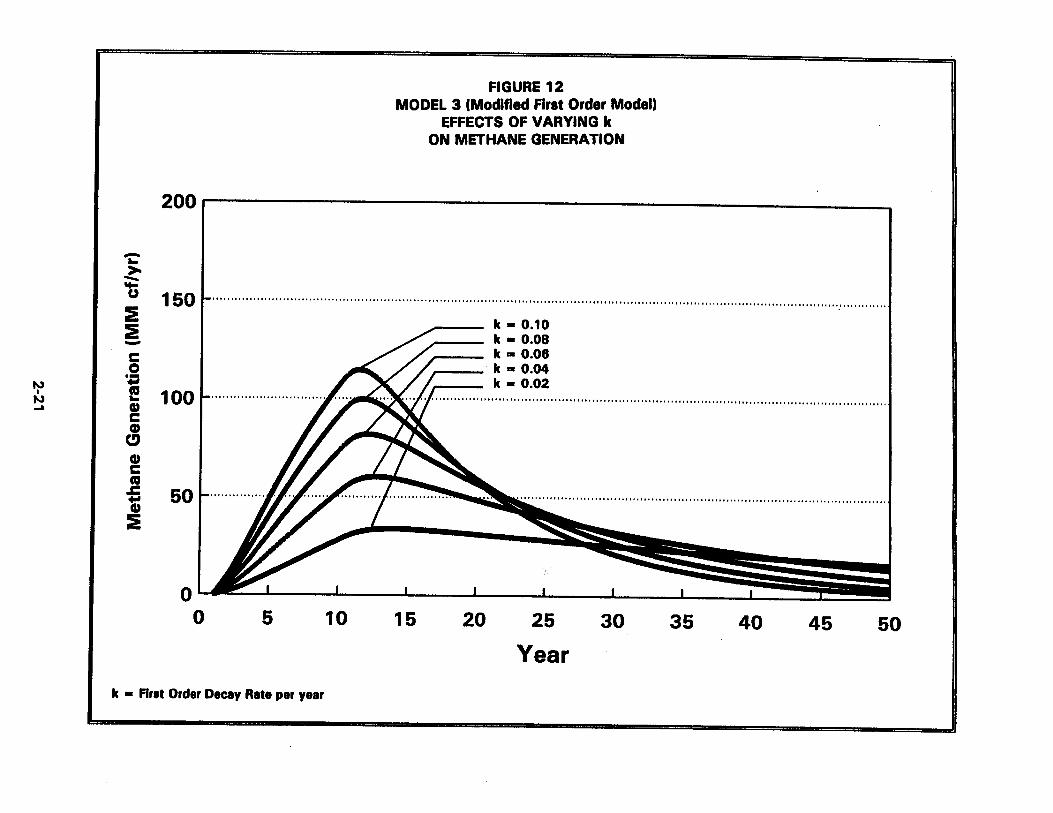
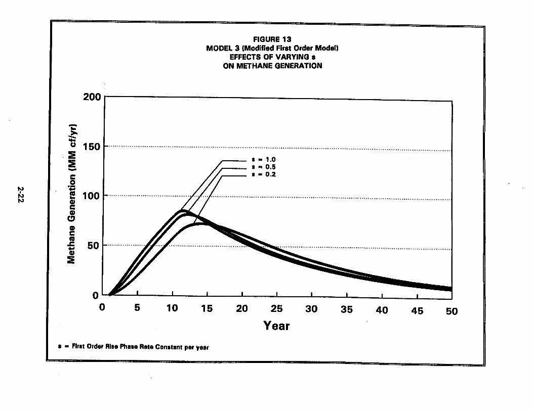
The Modified first Order Model has three parameters: the methane yield potential (Lo), the decay rate (k), and the rise phase constant (s). Sensitivity testing is illustrated as follows:

Figure 1 1 depicts the effects of varying Lo; Figure 12 depicts the effects of varying k; and Figure 13 depicts the effects of varying s.

The impact of varying Lo in Model 3, 8s with Model 2, is to increase generation proportionally to Lo. Effect of varying k in Model 3 is similar to the effect exhibited in Model 2. These results are not surprising, given similarities between Models 2 and 3.

Figure 13 depicts the effect of varying 's" in the Modified First Order Model. In this model, values for 's" fix the rate of rise in methane generation/recovery after filling. (As noted above, the justification for this model form is that such a rise from initially low rates of recovery is commonly observed in the field.) Figwe 13 shows the effect of the rise phase constant *s" on the time to reach peak generation, and the peak rate at which methane is generated. The rise phase constant also has a minor effect in the rate of decay from peak generation .

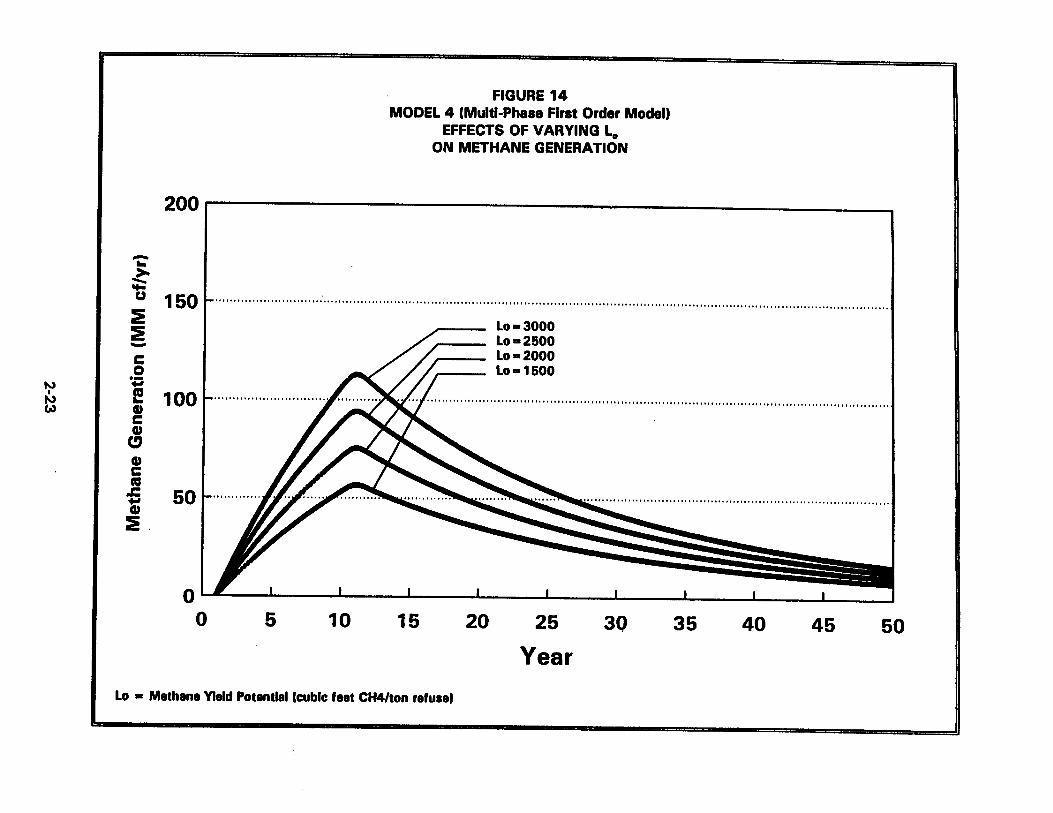
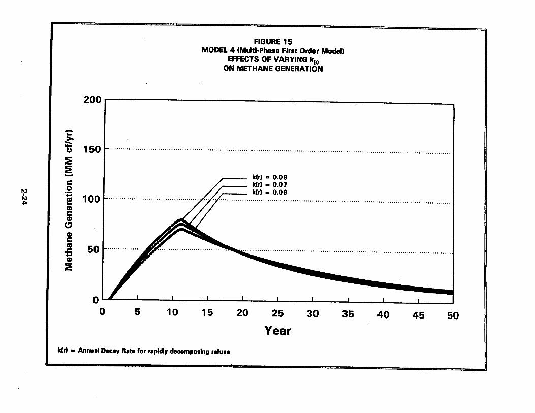
The Mutti-Phase First Order Model has four parameters: the methane yield potential (to); the fraction of rapidly decomposing refuse, F(r1; the decay rate of rapidly decomposing refuse, k(r); and the decay rate of slowly decomposing refuse, k(s).

A graphic summary of sensitivity testing for this model is summarized by parameter as fallows:

Figure 14 depicts the effects of varying Lo; Figure 15 depicts the effects of varying k(r); Figure 16 depicts the effects of varying k(s1; and Figure 17 depicts the effects of varying waste composition.

Methane recovery at any given time is directly proportional to Lo; that is, doubling the selected value for Lo will double the estimated peak generation rate. Of the two decay values, variations in k(r1 has a minimal effect on the generation pattern while changes to

2-9

k(s) have a more pronounced effect on model results.

As might be anticipated, Model 4 will be sensitive to changes in waste composition. As the selected value for F(s) is increased, peak generation (and time to reach this state) is decreased. However, the rate of tail-off in recovery is correspondingly less pronounced

. when a high fraction of slower decaying waste is assumed.

The procedures to estimate ‘best” values for model parameters and to allow comparisons between the four models ace discussed in Section 3.

2-1 0

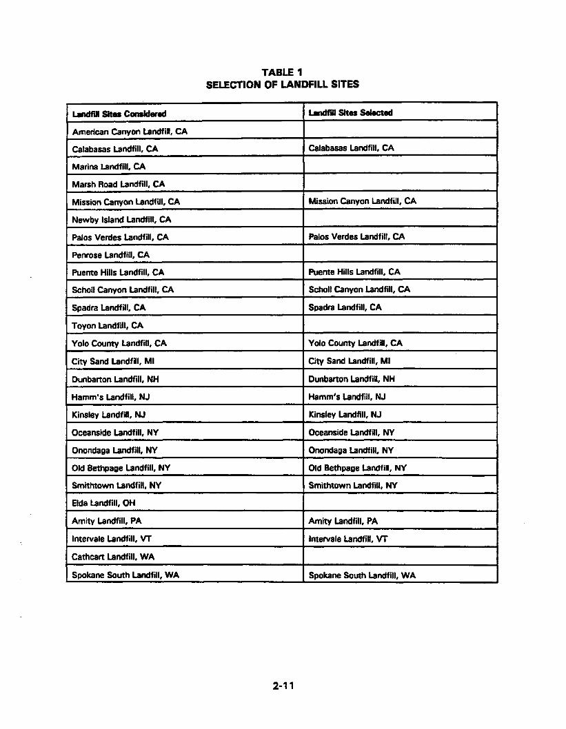
TABLE 1 SELECTION OF LANDFILL SITES

bndfill $itdm Coddered

American Canyon Landfilf, CA

Catabasas Landfill, CA

Marina landfitl, CA

Marsh Road Landfill, CA

Mission Canyon Landfill, CA

lautfinsites selected

Calabasas Landfill, CA

Mission Canyon Landfill, CA -

I ~~

Newby Island Landfill, CA

Cathcart Landfill, WA

Spokane South Landfill, WA

Palos Verdes Landfill, CA I Palos Verdes Landfill, CA

Spokane South bndfill, WA

I ~ ~~ _. . .- ~~~

Penrose Landfill, CA

Puente Hills Landfill, CA 1 puente Hills Landfill, CA

Schoil Canyon Landfill, CA I S ~ ~ O I I Canyon Landfill, CA ~~~

Spadra Landfill, CA 1 Spadra Landfill, CA

Toyon Landfill, CA I Yolo County Landfill, CA I yo10 county Landfill, CA

City Sand bndfill, MI I C i Sand Landfill, MI -- - ~

Dunbarton Landfill, NH I Dunbarton Landfilt, NH

Hamm's Landfill, NJ I tlamm's Landfill, NJ

Kinsley Landfill, NJ I Kinsley Landfill, NJ

Oceanside Landfill, NY I Oceanside landfill, NY

Onondaga Landfill, NY I Onondaga Landfill, NY

Old Bethpage Landfill, W I Old Bethpage Landfill, NY

Smithtown Landfill, NY

Elda Landfill, OH

Amity Landfill, PA Amity Landfill, PA

lntewale Landfill, VT 1 Intervale Landfill, VT

2-1 1

SECTION 3

APPROACH FOR MODEL OPTIMIZATION AND COMPARISON

OVERVIEW OF APPROACH

This section presents the approaches considered for model optimization and subsequent methods for model comparison. Model optimization sought to calibrate the selected landfill methane models through varying key model parameters to obtain the "best fit" to fiefd results for each model.

There can be different definitions of "best fit", and several approaches exist for this kind of data analysis and model calibration. Typical optimization functions are based on the differences (or residuals) between projected methane recovery and measured field data, or on the ratios of projected methane recovery to measured field data. Model optimization approaches considered for this study were:

a a 0

0 Minimization of arithmetic error:

Use of absolute filling and recovery data; Use of normalized filling and recovery data; Fitting of fillinghecovery data to trial models;

- use of absolute value of the differences; - use of square of the differences ke., least squares);

- use of the natural log of the ratios; - use of absolute value of the natural log of the ratios; and - use of square of the natural log of the ratios.

Minimization of logarithmic error:

Of these data treatment choices considered, two were selected for application and subsequent model comparisons in accordance with the scope of the study. The first calibration method was minimization of arithmetic error through use of the absolute value of the differences; the second method was minimization of logarithmic error through the use of the absolute value of the natural log of the ratios.

Minimization of arithmetic and logarithmic residuals has certain advantages and disadvantages. Minimization of arithmetic residuals weights according to actual waste quantities and gas recoveries. For example, large model errors at high recovery rates are more important than smaller model errors at lower recovery rates. in contrast, an advantage of the logarithmic optimization is in normalizing, so that both large and small landfills' data count equally. But, logarithmic optimization might give less weight to an important discrepancy between prediction and experience. For example, it will give equal weight to the log,, spreads between a 50,000 cfm predicted versus 5,000 cfm experienced ratio and to a 500 cfm predicted versus 50 cfm experienced ratio.

Another consequence of minimizing logarithmic rather than arithmetic residuals is that the optimized prediction will tend toward the log mean rather than the arithmetic mean of projections. For data with a significant amount of scatter, the log mean recovery may be

3-1

significantly less than the arithmetic. One consequence is that the model obtained by minimizing logarithmic residuals may underpredict recovery.

MODEL OPTIMIZAT10N PROCEDURE

Each model calibration method adjusted parameters for each of the four models to minimize model error (and thus, obtain one form of "best fit") between predictions of the trial model at hand and the gas recovery data set from the 18 landfills. The calibration methods weighted data in accordance with waste placement magnitude and methane recovery.

Modeled methane generation for a landfill site was assumed to be equivalent to methane recovery experienced. In addition, a time mesh or interval of one year for methane recovery was used for model optimization. Lastly, it was assumed that for each-landfill site, gas recovery during any one-year period would count as one value in the optimization process. Thus, landfills with fewer recovery values contributed less to the project results than landfills with more recovery values.

For minimization of arithmetic error, the model optimization procedure was:

Based on the waste filling history for each of the study landfills, establish parameter values for time (t) and waste in place (W). For each mod818 calculate methane generation (GI over time using a probable combination of remaining parameter values (e.g., k and Lo). (Parameters varied for each model were identified in Section 2.)

a Run iterative calculations of G over time for the varied parameters through small adjustments of the parameters over a wide range of numerical values. These iterations yield a series of model recovery projections, one for each combination of model parameters.

0 For each trial model and parameter combination leading to a projection, calculate the absolute arithmetic difference between the model projection data points for methane generation (GI and the experienced methane gas recovery from the study Landfill dataset.

Sum the arithmetic differences (or residuals) between projections and experienced methane recoveries for the study landfill to obtain a total "sum of residuals" or total arithmetic error. The "calibrated" (or optimized) model is simply the trial model form with parameter Combinations that give the minimum arithmetic error, and thus, the %st' predictions.

Procedures fur minimization of logarithmic error were similar to the above except that the logarithms of waste placement and gas recovery were used, and minimization was performed on the absolute values of the residuals (differences in the natural logs of the ratios of gas recovery predicted versus gas recovery experienced).

3-2

ILlUSTRATlON OF TRIAL MODEL OPTIMIZATION

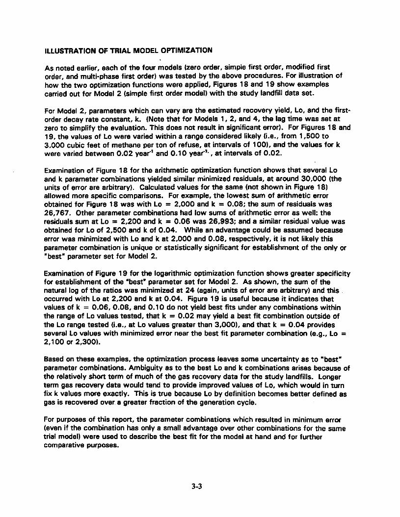
As noted earlier, each of the four models (zero order, simple first order, modified first order, and multi-phase first order) was tested by the above procedures. For illustration of how the two optimization functions were applied, Figures 18 and 19 show examples carried out for Model 2 (simple first order model) with the study landfill data set.

For Model 2, parameters which can vary are the estimated recovery yield, Lo, and the first- order decay rate constant, k. (Note that for Models 1, 2, and 4, the lag time was set at zero to simplify the evaluation. This does not result in significant error). For Figures 18 and 19, the values of Lo were varied within a range considered likely (i.e., from 1,500 to 3,000 cubic feet of methane per ton of refuse, at intervals of 1001, and the values for k were varied between 0.02 year-' and 0.10 year-'. , at intervals of 0.02.

Examination of Figure 18 for the arithmetic optimization function shows that several Lo and k parameter com binations yielded similar minimized residuals, at around 30,000 (the units of error are arbitrary). Calculated values for the same (not shown in Figure 18) allowed more specific comparisons. For example, the lowest sum of arithmetic error obtained for Figure 18 was with Lo = 2,000 and k = 0.08; the sum of residuals was 26,767. Other parameter combinations had low sums of arithmetic error as well: the residuals sum at Lo = 2,200 and k = 0.06 was 26,993; and a similar residual value was obtained for lo of 2,500 and k of 0.04. While an advantage could be assumed because error was minimized with Lo and k at 2,000 and 0.08, respectively, it is not likely this parameter com bination is unique or statistically significant for establishment of the only or "best" parameter set for Model 2.

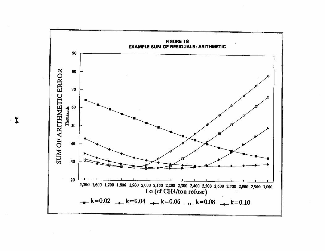
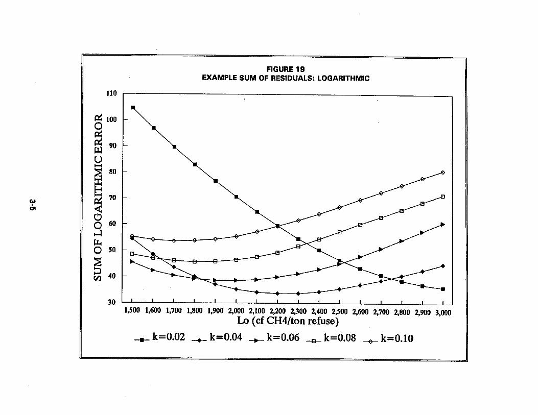
Examination of Figure 1 9 for the logarithmic optimization function shows greater specificity for establishment of the 'best" parameter set for Model 2. As shown, the sum of the natural log of the ratios was minimized at 24 (again, units af error are arbitrary) and this .

occurred with Lo at 2,200 and k at 0.04. Figure 19 is useful because it indicates that values of k = O.O6,0.08, and 0.10 do not yield best fits under any combinations within the range of Lo values tested, that k = 0.02 may yield a best fit combination outside of the Lo range tested (i.e., at Lo values greater than 3,0001, and that k = 0.04 provides several Lo values with minimized error near the best fit parameter combination (e.g., Lo = 2,100 or 2,300).

Based on these examples, the optimization process leaves some uncertainty 8s to "best" parameter combinations. Ambiguity as to the best Lo and k combinations arises because of the relatively short term of much of the gas recovery data for the study landfills. Longer term gas recovery data would tend to provide improved values of Lo, which would in turn fix k values more exactly. This is true b8cause Lo by definition becomes better defined as gas is recovered over a greater fraction of the generation cycle.

For purposes of this report, the parameter combinations which resulted in minimum error (even if the combination has only a small advantage over other combinations for the same trial model) were used to describe the best fit for the model at hand and for further corn parative purposes.

3-3

SECTION 4

RESULTS

PARAMETER COMBINATIONS DERIVED FROM MINIMIZED ERROR

Numerous computer runs were made to calculate the residuals for possible parameter corn binations for:

the ranges of parameter values selected;

0 the four models and 18 landfill sites evaluated in this study; and .

the two optimization functions selected.

R8Sults from these computer runs were scanned visually for optimal results and compared numerically for the lowest minimized error. fable 2 presents the resulting parameter combinations by landfill methane model and by optimization function. Application of the data treatment of absolute vaIue of the logarithmic error produced two different parameter combinations (each had an equivalent lowest minimized error) under each of Models 1, 2, and 3.

As indicated in Table 2, values for to, the methane yield potential, were consistent for the three first-order models (i.e., Models 2, 3, and 4) under the arithmetic error optimization function, ranging from 2,100 to 2,200 cubic feet of methane per ton of landfilled waste. Under the logarithmic function, at least one parameter combination for each of the four models resulted in an Lo within the 2,000 to 2,200 cubic feet of methane range.

Values for k, the first order decay rate constant, were more varied and model dependent. Under the arithmetic optimization function, k values ranged from O.OS/year to O.OS/year for Models 2, 3, and 4; under the logarithmic optimization function, k values ranged from O.OS/year to O.OG/year.

MODEL COMPARISONS

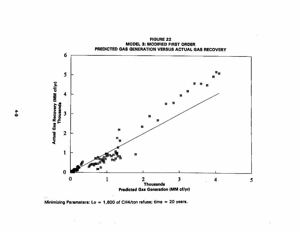
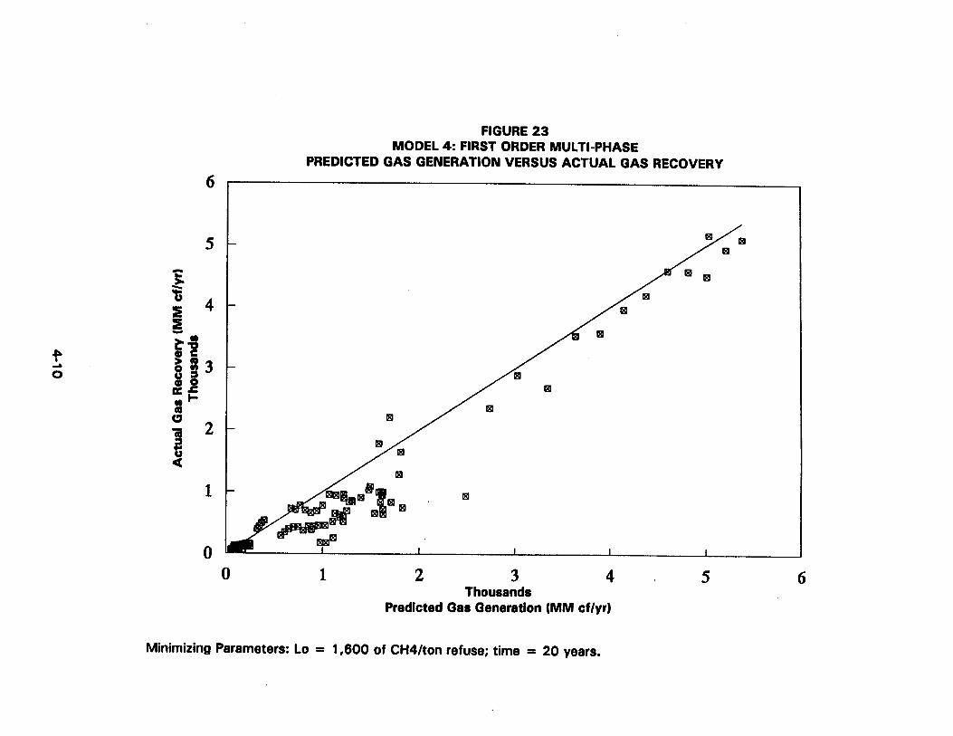
Comparisons of the study landfill data to the optimized (or best fit) models were developed. tn brief model parameter combinations obtained through minimization of arithmetic residuals (see Table 2) were used to develop generation curves; these data sets then were plotted against the actual methane recovery data from the 18 study landfills. Results of these plots are shown in Figures 20 through 23 for Models 1 through 4, respectively. In these figures the fit of each model is illustrated by comparison of optimized model predictions for methane generation with the measured methane recovery for atJ data points obtained from the study landfills. The model parameter cornbinations from Table 2 used to develop the predicted methane generation data ke., the x-axis) are shown on the figures as well.

4-1

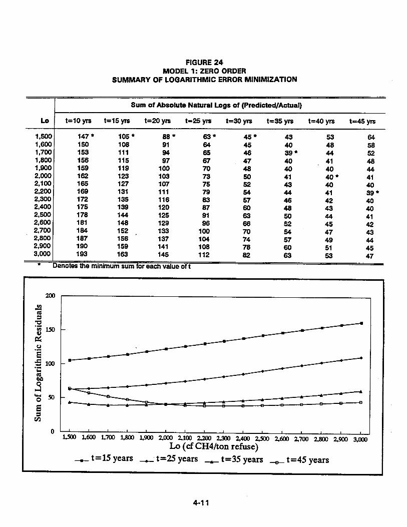
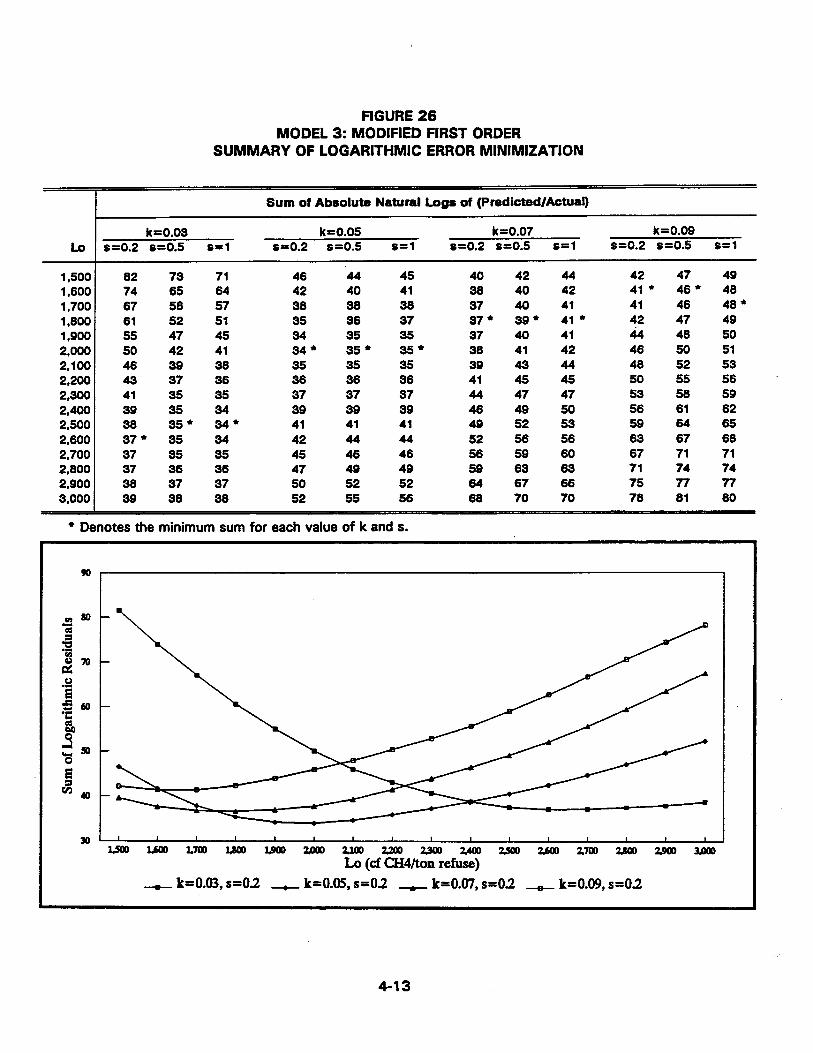
Similarly, comparisons were made for each of the four models to show the results of Optimization via minimization of logarithmic tesiduats, as described in the previous section. Figures 24 through 27 provide tabular and graphic results from the optimization procedure for Models 1 through 4, respectively. The parameter combinations derived from minimizing logarithmic error (given for each model in Table 2) are indicated on the figures as well.

This use of differing weighting yielded, in several cases, similar parameter combinations to the arithmetic results. Furthermore, minimization of logarithmic error gave better results than those demonstrated by arithmetic error minimization by producing a narrow, more specific band of parameter combinations for best fit optimization. As a result, other combinations could be eliminated. For example, parameter combinations which included vaiues of t = 15 years and t = 25 years for the zero order model (Model 1) clearly could not result in the lowest minimized error (see Figure 24). The same conclusion could be drawn for parameter combinations which included:

Values of k = 0.07,0.08,0.09, and 0.10 for Model 2 (see Figure 25);

Values of k = 0.07 and 0.09 for Model 3 (see Figure 26); and

0 Values of k(r) and k(s) = 0.06, k(r) = 0.07 and k(s) = 0.06, and k(r) = 0.08 and k(s) = 0.06, for Model 4 (see Figure 27).

Figures 20 through 23 also allow model comparisons of predicted versus actual methane recovery in terms of the variance of landfill data points from the straight line (the straight line represents an exact correlation). A commonly-applied statistical measure for good correlation or "goodness of fit" for modeled data is the regression coefficient, r2. Regression coefficients were calculated for the plots shown in Figures 20 through 23 (based on arithmetic optimization) and for similar data based on logarithmic optimization. Results are presented in Table 3.

Generally, regression coefficient values based on arithmetic optimization were similar for all four models, ranging from 0.928 to 0.937, depending on the model. This could be considered reason8 ble correlation. By one interpretation, such a regression coefficient might indicate that from 92.8 to 93.7 percent of the variation in methane recovery could be attributed to parameter values and inputs of the optimized model. Table 3 shows that regression coefficients for the logarithmic data treatment showed high correlations as well, ranging from 0.91 4 to 0.955. Similarity of the regression coefficient results indicates that the four models are similar in predictive ability.

However, the assumptions implicit in the use of the regression coefficient may not correspond exactly to landfill methane modeling. Where the regression coefficient is applied, an assumption is that an underlying "true" model exists, correlated to the extent

4-2

indicated by r2 t o model variables. Deviations between the model prediction and measured methane recovery are otherwise assumed to be due to unknown factors or random errors (such as in field measurements made).

This base assumption may not be valid if I much higher fraction of the discrepancy between the modeled and experienced values is not random, but due to unquantified real biases. An example of such bias that could show as "random" error would be where one landfill yields much greater methane recovery over time (essentially, a greater lo value) than another because of greater moisture infiltration and distribution within the waste mass.

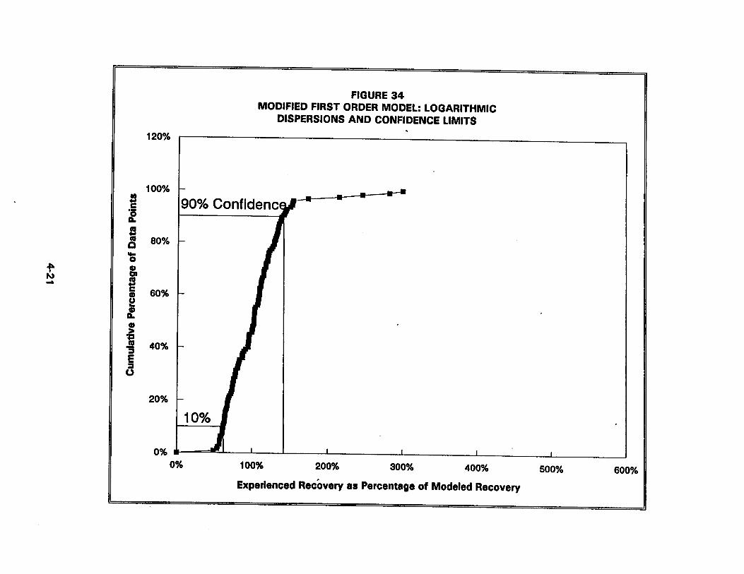
The four landfill methane models also were compared through examination of data distributions of the numerical ratios of the measured methane recovery values to the modeled recovery over the spectrum of data points established for the study landfills. For each model and each optimization function (arithmetic and logarithmic), plots were developed to show distributions around median values for modeled versus actual methane recovery values . Figures 28 through 31 provide distribution plots for Models 1 through 4, respectively, based on the minimization of arithmetic error. Similarly, Figures 32 through 35 provide distribution plots for Models 1 through 4, respectively, based on the minimization of logarithmic error.

For these figures, a "perfect" model correlation would be represented by a vertical line of the landfill data points at 100 percent of actual recovery (the x-axis). Data 'scatter" or dispersion from perfect correlation are illustrated on the figures with bounds shown by vertical lines. These bounds represent the 10 and 90 percent probability (or confidence) limits. In other words, the cumulated fraction of points lying within any particular boundary, in terms of percentages of the modeled prediction, indicates the dispersion of experienced recovery about the model prediction.

Overall, Figures 28 through 35 show rather wide probability limits for the set of study landfills, meaning the models could project methane recovery within a factor of about 1.5 fur 80 percent of the landfill data points. The spread or dispersion was greater for the remaining data points. Note that this is the first time that methane recovery probability limits have been developed in association with projections for U S . landfills. (Where landfills share common filling histories and operational features, a narrower range for the limits might be expected).

Comparison of the two groups of figures representing arithmetic versus logarithmic data treatments (Figures 28 through 31 and Figures 32 through 358 respectively) indicates that the probability limits for the models optimized via logarithmic minimization are narrower than those established with the arithmetic optimization.

4-3

Of w e 1 P a w s With Otfier Work

Parameter combinations developed for the study landfill data set were compared in a timited manner with other published values. As shown in Table 2 for the Simple First Order Model (Model 21, study tandfill results had three parameter combinations associated with minimized error: Lo = 2,100 and k = 0.07/year; Lo = 2,200 and k = 0.04/year; and Lo = 2,500 and k = 0,03/year. The U.S. €PA has published regulatory values based on reported literature values for Lo and k and its first order landfill methane emissions model. The regulatory values are t o = 4,010 cubic feet methane per refuse ton, k (for wet sites) = 0.04, and k (for dry sites) = 0.02, from Camallatran of Air Po-n F m

v Paint and Area SourceS, July 1993 (AP-42). t t is assumed that EPA's Lo value was selected to be higher than reported typical landfill values in order to be conservative for regulatory purposes.

. . . .

For other published model work, some interpretive calculations were made to compare with this work's findings. Fur example, Oonk, et. al. (1994) based methane yield on an assumed waste degradable carbon content. 8ased on average Dutch waste composition, the first order Lo from Oonk can be calculated to be about 2,200 cubic feet of methane per ton, and a first order rate constant, k, of O.Og/years.

Another commercial model reported by Augenstein (1 992) and (Augenstein and Pacey, 199 1 ) based projections on dry waste of assumed composition. An assumed 25 percent waste moisture content for this model gave an Lo value 2,100 cubic feet of methane per ton, and k values near 0.07/year.

P ul

TABLE 2 METHANE MODEL PARAM€TER COMBINATIONS YlELDlNO MINIMIZED ERROR

Optimization Function

1. Minimization of Absolute Value of Arithmetic Error

II. Minimization of Absolute Value of Logarithmic Error

Model 1: Zero Order

LO = 1,600

t = 20 years

LO = 1,700

t = 35 years

AND

Lo = 2,200

t = 45 years

Parameter ComMnations+

Model 2: Simple First Order

Lo = 2,100

k = 0.07lyear

Lo = 2,200

k = 0.04/year

AND

LO = 2,500

k = 0.03/year

Model 3: Modified First

Order

Lo = 2,200

k = O.05lyear

8 = 1.0

Lo = 2,000

k = O.OB/year

8 = 0.2

AND

LO = 2,500

k = O.OS/year

s = 1.0

Modei 4: Firat Order Multi-

Phase

Units for Lo, methane yield potential, are cubic feet methane gas per ton of waste landfifled.

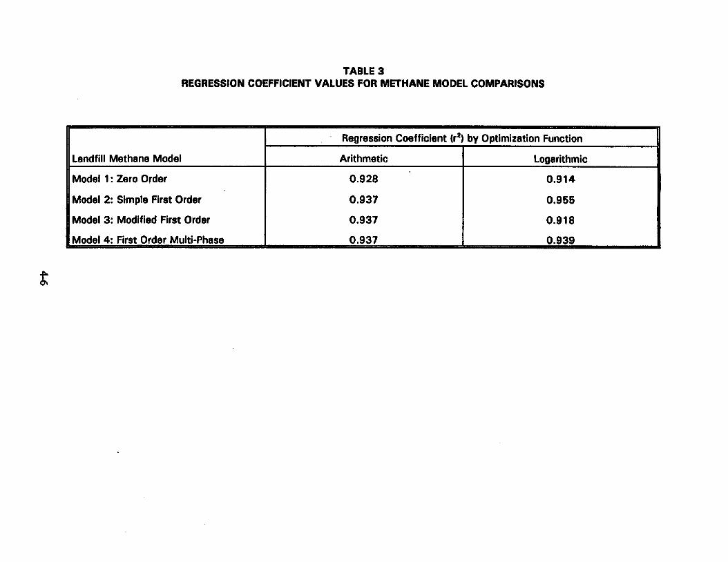
TABLE 3 REGRESSION COEFFICIENT VALUES FOR METHANE MODEL COMPARISONS

I * Regression Coefficient (r2) by Optimization Function

Landfill Methane Model I Arithmetic I Looarithmic

Model 1: Zero Order 0.914

Model 2: Simple First Order 0.955

Model 3: Modified First Order 0.918

SECTION 5

COMPUTER PROGRAM FOR LANDFILL METHANE MODELS

Based on this report's findings, a simple computer program was developed for each of the four models discussed herein. r i led as 'Methane Gas Recovery Program (MEGAREP), Version 1 1 ", the program presumes a landfill has characteristics typical of the study landfills. This program is included herein as a diskette in Appendix C.

MEGAREP accepts keyboard data to a standard spreadsheet application (Cod @ Quattro Pro *, version 6.0). The file can be read into similar spreadsheet programs. User inputs include landfill site name, the landfill waste filling history on an annual basis (i.e., tons of waste per year), and parameter combinations for each selected model. The user can input model parameter combinations from Table 2 (as derived from the report's procedures to optimize models through minimization of error), or other parameter cornbinations as desired.

MEGAREP outputs from each of the four models are tabular data and plots for estimated methane generation over time, For purposes of the program, methane generation estimates were treated as equivalent to expected methane recovery. Other program outputs are probability limits (or uncertainty bounds). The probability limits (upper and lower bounds) are calculated (tabular data) and piotted for the simple first order model (Model 2). These limits are based on the minimization of arithmetic error procedures described in the report. Example input forms and program outputs for the four models are presented in Appendix C.

Probability limits are expressed in terms of the likelihood of seeing predicted gas recovery levels. For example, model outputs provide expected gas recovery levels that would be seen 90 percent of the time, 50 percent of the time, and 10 percent of the time. Users can decide what limits ate reasonable or acceptable as the basis for design and siting of 8 landfill gas collection and recovery system.

Note that this is the first time that methane recovery probability limits have been available in association with projections for US. landfills.

5=1

SECTION 6

RECOMMENDATIONS FOR FURTHER WORK

This section recommends further work that could be carried out to improve the utility and confideme limits of the landfill methane models discussed herein.

1. Develop More Complete Landfill Site Characterization

Notwithstanding past results,' more detailed site data from study landfills should help to improve modeling accuracy. landfill site characterization inf omation WBS considered in questions of the project questionnaire (Appendix B), Except for the Sanitation Districts of Southern California landfills, limited information was obtained from the study landfills other than gate waste tonnage and methane recovery information, In other projects, an interview and inf orrnation exchange process has been successf uf in eliciting additional detailed information (U.S. €PA, 1995). Should additional site information be developed for the study landfills to test for improved correlations, the conduct of follow-up intenhews is recommended.

2. Continue Accumulation of Data for Study Landfills

Collection of study landfills' data should continue, particularly waste filling and methane recovery information. Working relationships established with the landfill owners/operators should help with collection of future data 8s they become available. Such future data will better define "real" parameter combinations; that is, those that best explain the long-term methane generation/recOvery profile.

3. Add More Landfills to the Study Data Set

Addition of landfills to the study's data set will expand the usefulness and application of the model comparisons. Furthermore, model calibration is needed for groups of landfills located in distinct geographWclimate regions. A larger data set should allow better evaluation for such groups of landfills, such as those in Eastern regions and hot, humid climate regions.

4. Examine Other Data Treatment Approaches

Four landfill methane models were compared through the use of two optimization functions. Other optimization functions were identified but not applied (such as

6-1

minimization of arithmetic error by least squares, minimization of logarithmic error by the natural log of the ratios or the square of the natural log of the ratios). These choices for data treatment may be a useful step to further compare methane models and to better distinguish predictive abilities.

5. Examine Other Landfill Methane Models

Other trial model forms could be examined similar to the procedures pf8Sented in the study. Examples include multi-phase zero-order and second order models. It is possible that other models could be better in terms of reducing the discrepancies between model projections and field experience.

6. Incorporate Estimates For Methane Recovery Efficiency

The landfill methane models examined treated methane generation as equivalent to methane recovery; estimates for actual methane recovery efficiencies are not model parameters. Because recovery efficiency can affect significantly the sctual methane recovered, users of methane models should be experienced and familiar with LFG collection systems so as to apply proper judgement to the model results obtained. Incorporation of the parameter, methane recovery efficiency, to the study's computer program (MEGAREP, v. 1 .I ) is recommended as an initial step to allow users of methane models to discount predicted methane generation as appropriate.

6-2

SECTION 7

REFERENCES

Augenstein, 0. and 3. Pacey. 1991. Landfill Methane Models. Proceedings, SWANA 14th Annual International Solid Waste Symposium, Cincinnati, OH.

Atpem, R. 1973. Decomposition Rates of Garbage in Existing Los Angeles Landfills. Masters Thesis, California State University, Long Beach, CA.

Bariaz, M. A,, R. K. Ham, and 0. M. Schaefer. 1990. Methane Production from Municipal Refuse: a Review of Enhancement Techniques and Microbial Dynamics. Critical Reviews in Environmental Control, 19 pp. 557-584.

EPRl (Electric Power Research institute). 1992. Survey of Landfill Gas Generation Potential: 2 MW Molten Carbonate Fuel Cell. Report EPRl TR-101068. Electric Power Research Institute, Pal0 Alto, CA- ,

Farquhar, G. .I. and S.A. Rovers. 1973. Gas Production from Landfill Decomposition. Water, Soil and Air Pollution 2, 493.

Halvadakis, C. P., A. 0. Robertson, and J. Leckie. 1983. Landfill Methanogenesis: Literature Review and Critique. Stanford University Civil Engineering Report No. 271. Available from NTIS.

Ham, R. K., K. K. Hekemian, S. L. Katten, W. J. Lockman, R. J. Lofy, D. E. McFaddin, and E. J. Daley. 1979. Recovery, Processing and Utilization of Gas from Sanitary Landfills.

Ham, R. K. 1979. Predicting Gas Generation from Landfills.

Oonk, J., A. Weenk, 0. Coops, and L. Luning. 1994. Validation of Landfill Gas Formation Models. Institute of Environmental and Energy Technology, Report No. 94-31 5.

Peer, R. L., D. L. Epperson, D. L. Campbell, and P. Von Brook. 1992. Development of and Empirical Model of Methane Emissions from Landfills. U.S. EFA, Office of Research and Development.

U. S. EPA. 1993. Opportunities to Reduce Anthropogenic Methane Emissions in the United States. Report No. EPA 430-R-93-012.

Van Zanten, 8. and M. J. 3. Scheepers. 1995. Modelling of Landfill Gas Potentials. Proceedings, SWANA 18'" Annual Landfill Gas Symposium, New Orleans, LA.

Walsh, J. J. 1994. Preliminary Feasibility Investigation for LFG Recovery. Identification and interpretation of Site Background Data. Proceedings, SWANA 17"' Annual Landfill Gas Symposium, Long Beach, CA.

Zison, S. 1990. Production Curves: Myths versus Reality. Presentation at GRCDASWANA Solid Waste Symposium, Vancouver, B. C.

7-1

APPENDIX A

PROJECT LANDFILL SITE DATA

LANDFILL A WASTE PLACEMENT DATA

~

Methane Refuse Rmcovery

Year (To Wyear) (MM eflyear)

1955 1956 1957 1958 1959 1960 1961 1962 1963 1964 I965 1966 1967 1968 1969 t 970 1971 1972 1973 1974 1975 1 976 1977 1978 1979 1980 1981 1982 1983 1984 1985 1986 1987 1988 1989 1990 1991 1992 1993 1994 1995

31 0,000 31 0,000 31 0,000 31 0,000 31 0,000 31 0,000 31 0,000 31 0,000 31 0,000 470,000 470,000 470,000 470,000 720,000 750,000 770,000 800,000 830,000

1,260,000 1,490,000 1,530,000 1,050,000

870,000 900,000

1,200,000 1,700,000

850,000

652 637

1,281 1,637 2,201 1,776

A-2

IANDFIU B WASTE PLACEMENT DATA

Year

Methane Refuse Recovery

(Tons/year) (MM &/year)

1955 1956 1 957 1958 1959 1960 1961 1962 1963 1964 t 965 1 966 1967 1968 t 969 1970 1971 1972 1973 1974 1975 1 976 1977 1 978 1 979 1980 1981 1982 1983 1984 1985 1986 1987 1980 1989 1990 1991 1992 1993 1994 1995

21 3,000 232,000 232,000 232,000

232,000 508,000 71 1,000

1 ,I 14,000 1,265,000 1,528,000 1,484,000

593,000 287,000 41,000

232,000

179 180 441 443 373 433 426 400 344 293

A-3

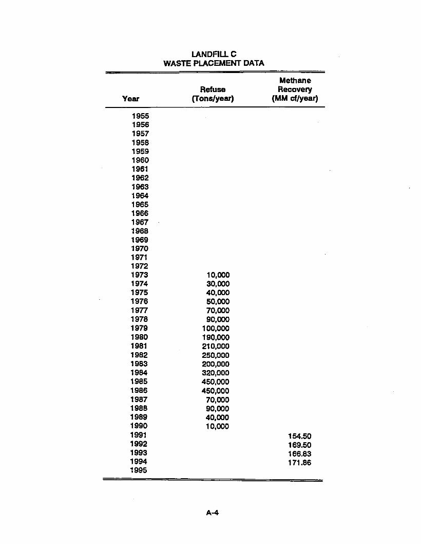
IANDFIU C WASTE PLACEMENT DATA

Methane Refuse Recovery

Year (Tondye=) (MM cf/year)

1955 1956 1957 1958 1959 1960 1961 1962 1963 1964 1965 1966

1968 t 969 1970 1971 1 972 1973 1974 1 975 t 976 1977 1978 1 979 1980 1981 1982 1983 1984 1985 1986 1987 1988 1989 1990 1991 1992 1993 1994 1995

1967 .

10,000 30,000 40,000 50,000 70;w0 90,000

100,000 190,000 21 0,000 250,000 200,000 320,000 450,000 450,000

70,000 90,000 40,000 10,000

154.50 169.50 166.83 171.86

LANDFILL D WASTE PLACEMENT DATA

Methane Ref use Recovery

Year (Tons/ye=) (MM cf/year)

1955 1956 1957 1958 1959 1960 1961 1962 1963 1964 1965 1966 1967 1968 1969 t 970 1971 1 972 1973 1974 1975 3 976 1977 1978 1 979 1980 1981 1982 1983 19&4 1985 1986 1987 1988 1989 1990 1991 1992 t 993 1994 1995

24,000 25,000 27,000 74,000 72,000 74,000 77,000 82,OOO 82,000 88,000 94,000 99,000

105,000 109,000 108,000 100,000 100,000 69,000 63,000 62,000 60,000

88.44 60.20 85.39 70.89 72.07 89.1 9

A-5

UNDFILL E WASTE PLACEMENT DATA

Year

Methane Refuse Recovery

CToWYe@ (MM &/year)

1955 1956 1957 1958 1959 1960 1961 1962 1963 1964 1965 1966 1967 1968 1969 1970 1971 1 972 1 973 1 974 1975 1976 1977 1878 1979 1980 1981 1982 1983 1984 1985 1986 1987 1988 1989 t 990 t 991 1992 1993 1994 1995

10,000 30,000 40,000 50,000 70,~0 90,000

100,000 190,000 21 0,000 250,000 200,000 320,000 450,000 450,000 70,000 90,000 40,000 10,000

1 12.67 11 8.44 11 8.44 1 19.63

A-6

LANDFILL F WASTE PLACEMENT DATA

~

Methane Refuse Recovery

Year Crons/ye=) (MM cf/year) ~ ~ ~ ~~

1955 I956 1957 1958 1959 1960 1961 1962 1963 1964 1965 1966 1967 1968 1969 1 970 1971 1972 1973 1974 1975 1976 1977 1978 1979 1980 1981 1982 1983 1984 1985 1986 1987 1988 1989 1990 I991 1992 1993 1994 1995

26,000 27,000 27,000 28,000 28,000 29,000 30,000 30,000 31,000 32,000 32,000 33,000 34,000 34,000 35,000 36,000 36,000 37,000 38,000 39,000 39,000 40,000 41,000 46,000 38,000

66.83 61 39

A-7

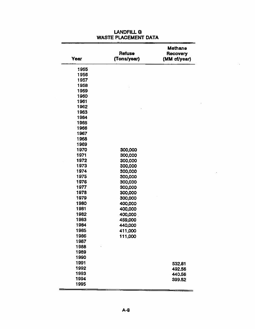
LANDFILL G WASTE PLACEMENT DATA

Year

Methane Refuse Recovery

CTonS/p-) (MM cf/year)

1955 1956 1957 1958 1959 1960 1961 1962 1963 1964 1965 1966 1967 1968 1969 1970 1971 1 972 1973 1974 1 975 1976 19n 1978 1979 1980 1981 1982 1983 1984 1985 1986 1987 1988 1989 1990 1991 1992 1993 1994 1995

300,000 300,000 300,000 300,000 300,000 300,000 300,000 300,000 300,000 300,000 40~,000 4 ~ 0 , O o ~ 400,000 . 459,000 440,000 41 1,000 11 1,000

532.81 492.56 440.56 399.52

A-8

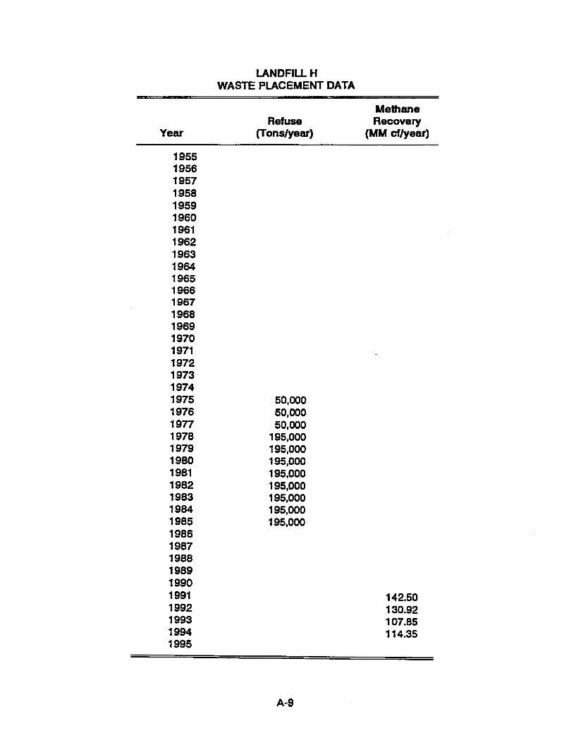
LANDFILL H WASTE PLACEMENT DATA

~~ ~~

Methane Refuse Recovery

Year Crans/year) (MM &/year)

1955 1956 1957 1958 1959 1960 1961 1962 1963 1964 1965 1966 1967 1968 1969 1970 1971 1972 1973 1974 1975 1976 1977 t 978 1 979 1980 1981 1982 1983 I984 1985 1986 1987 1988 1989 1990 1991 1992 1993 1994 1995

50,000 50,000 50,000

195,000 195,000 195,000 195,000 195,000 195,000 195,000 195,000

142.50 130.92 107.85 114.35

A-9

. .

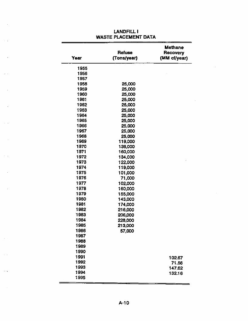
IANDFILL I WASTE PLACEMENT DATA

Year

Methane Refuse Recovery

(TOndy-) (MM &/year)

1955 1956 1957 1958 1959 1960 1961 1962 1963 1964 1965 1966 I967 1968 1969 1970 1971 1972 1973 1 974 1 975 1976 1977 1978 1979 1980 1981 1982 '1 983 1904 1985 1986 1987 1988 1989 1990 1991 1992 1993 3 994 1995

25,000 25,000 25,000 25,000 25,600 25,000 25,000 25,000 25,000 25,000 25,000

1 19,000 138,000 160,000 134,000 122,000 1 19,000 1ot,ooo 71,000 102,000 160,000 155,000 143,000 174,000 21 6,000 206,000 228,000 21 3,000 57,000

102.67 71.56 147.62 132.1 6

A-1 0

i

LANDFILL L WASTE PLACEMENT DATA

Methane Refuse Recovery

Year Cron dye=) (MM Wyear)

195s 1956 1957 1958 1959 1960 1961 1962 1963 1964 1965 1966 1967 1968 1969 1970 1971 1972 1973 1 974 1 975 I 976 1977 1978 1979 1980 1981 1982 1983 1984 1985 1986 1987 1988 1989 1990 1991 1992 1993 1994 1995

34000 669000 379000 51 9000 929000

115 131 111 1 07 79 72 67 62 66 72 65 59

A-1 3

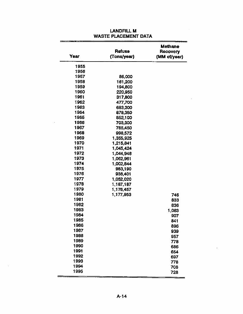
LANDFILL M WASTE PLACEMENT DATA

Year

Methane Recovery Refuse

VOnS/par) (MM cf/year)

1955 1956 1957 1958 1959 1960 1961 1962 1963 1964 I965 1966 1967 1968 1969 1970 1971 1972 1 973 1974 1975 1976 1977 1978 1979 1980 1981 1982 1983 1984 1985 1986 1987 1988 1989 1990 1991 1992 1993 1994 1995

86,000 161,200 194,800 220,950 31 7,800 477,700 683,300 878,350 852,100 703,500 785,450 998,572

1,355,925 1 $1 5,841 1,045,424 1 ,O44,W8 1,062,961 1,002,844

983,190 936,401

1,052,020 1 ,I 87,187 1 ,176,457 1 ,I 77,953 746

833 836

1,083 907 841 896 939 957

686 654 697 778 708 728

na

A-1 4

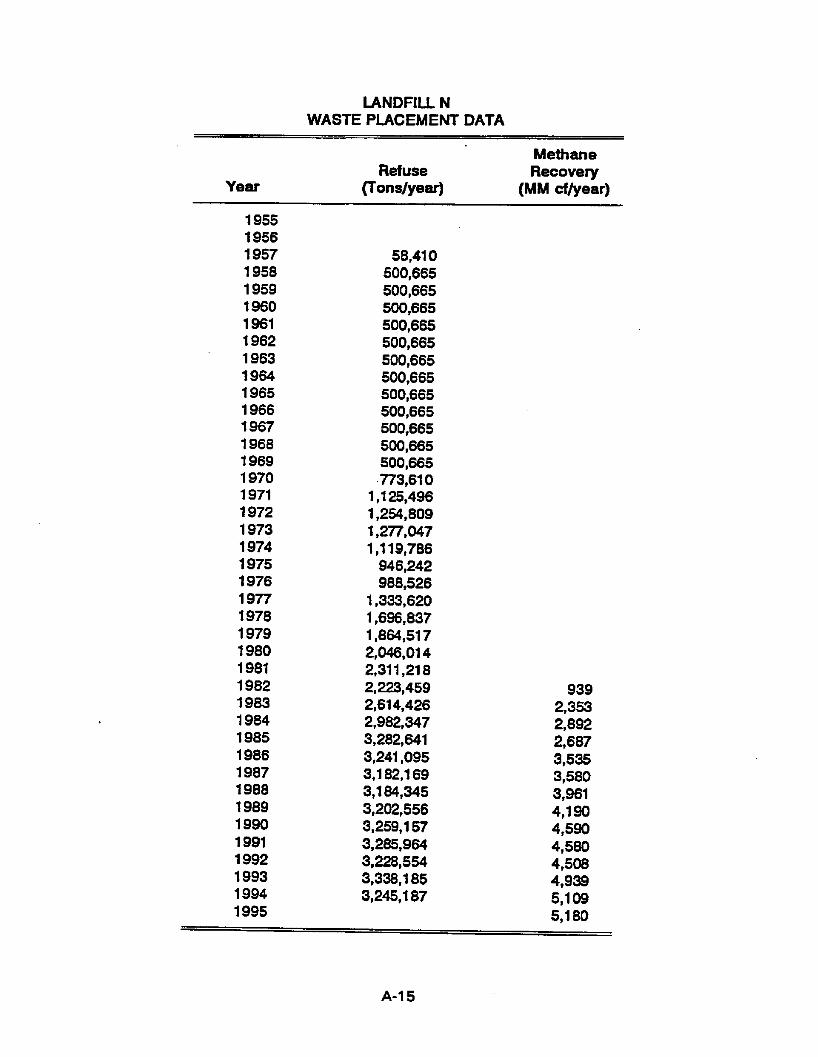
LANDFILL N WASTE PLACEMENT DATA

Year

~~

Methane Refuse Recovery

(To Wpar) (MM &/year)

1955 1956 1957 1958 1959 1960 1961 1962 1963 1964 1965 1966 1967 1968 1969 1970 1971 1972 1973 1 974 1 975 1976 1977 1978 1979 1980 1981 1982 1983 1984 1985 1986 1987 1988 1989 1990 1991 1992 1993 1994 1995

58,410 500,665 500,665 500,665 500,665 5 0 0,6 6 5 500,665 500,665 500,665 500,665 500,665 500,665 500,665

1 ,I 25,496 1,254,809 1,277,047 1,119,786

946,242 988,526

1,333,620 1,696,837 1,864,517 2,046,Ol 4 2,311,218 2,223,459 2,614,426 2,982,347 3,282,641 3,241,095 3,182,169 3,184,345 3,202,556 3,259,157 3,285,964 3,228,554 3,338,185 3,245,187

. 773,610

939 2,353 2,892 2,687 3,535 3,580 3,961 4,190 4,590 4,580 4,508 4,939 5,109 5,180

A-1 5

lANDFfLL 0 WASTE PLACEMENT DATA

Methane Refuse Recovery

Year (Tonslyeat) (MM d/year)

1955 1956 1957 1958 1959 1960 1961 1 962 1963 1964 1965 1966 1967 1968 1969 1970

, I971 1 972 1 973 1974 1975 1976 I977 1978 1 979 1980 1981 1982 t983 1984

1986 1987 1988 1989 1990 1991 1992 1993 1994 1995

1985

205,000 334,000 394,000 481,000 493,000 495,000 51 2,000 4 95,OO 0 499,000 475,000 458,400 453,000 431,000 462,000 493,000 440,700 498,500 61 0,300 691,400 750,800 81 7,500 867,700 895,300 879,000

1,062,900 1,527,100 1,620,200

683,900 763,012 673,625 6 5 3,6 9 7 607,714 61 1,901 532.240

_. -

71 8 993 942 952

1,002 995

1,032

A-16

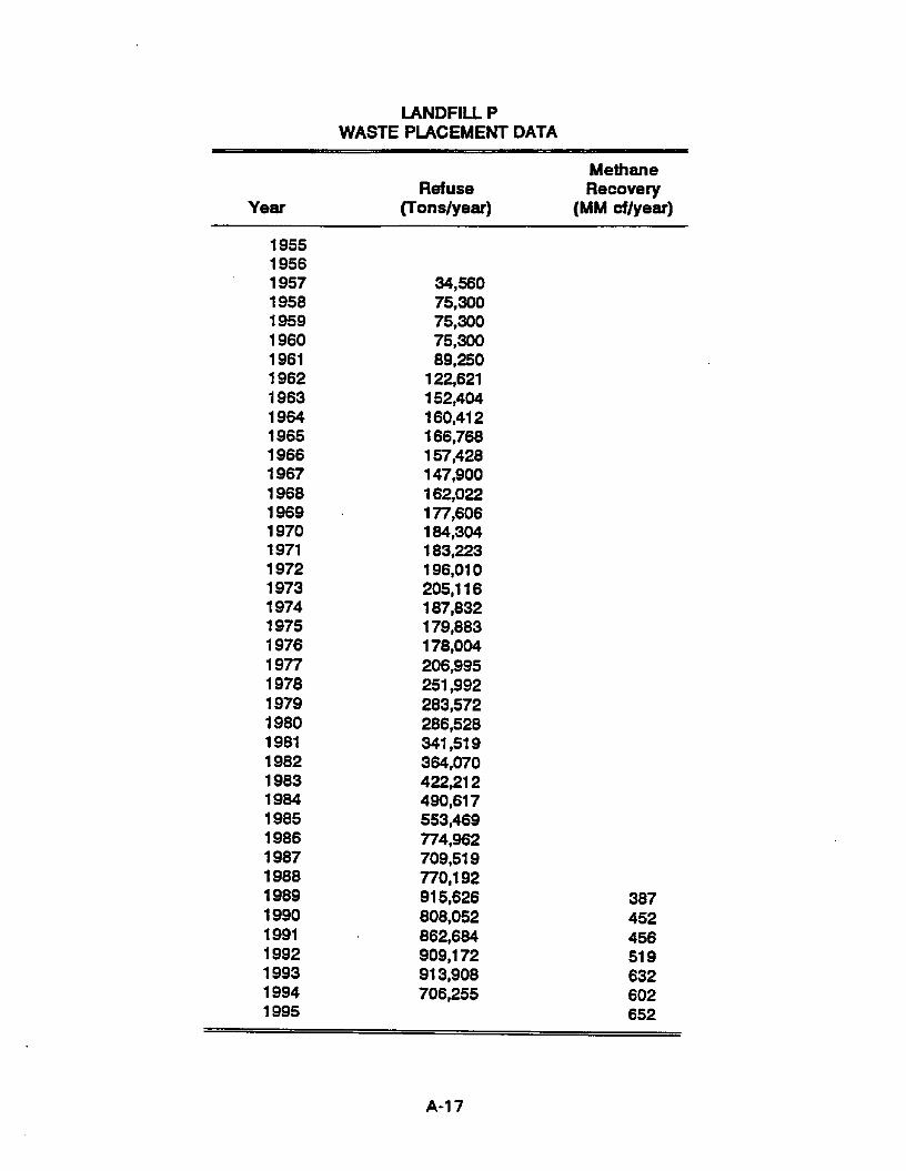
LANDFILL P WASTE PLACEMENT DATA

Year

~

Methane Ref use Recovery

Crons/year) (MM cf/year)

1955 1956

' 1957 1958 1959 1960 1961 1962 1963 1964 1965 1966 1967 1968 1969 1970 1971 'I 972 1973 1974 1 975 1976 1977 1978 1 979 I980 1981 1982 1983 1984 1985 1986 1987 1988 1989 1990 1991 1992 1993 1994 1995

34,560 75,300 75,300 75,300 89,250

122,621 152,404 160,412 166,768 157,428 147,900 162,022 177,606 184,304 183,223 196,010 205,t 16 187,832 179,883 178,004 206,995 251,992 283,572 286,528 341,519 364,070 422,212 490,617 553,469 774,962 709,51 9 770,192 91 5,626 808,052 862,684 909,172 91 3,908 706,25 5

387 452 456 51 9 632 602 652

A-1 7

LANDFILL Q WASTE PLACEMENT DATA

Year

Methane Refuse Recovery

(Tonslyear) (MM &/year)

1955 1956 1957 1958 1959 1960 1961 1962 1963 1964 1965 1966 1967 1968 1969 1970 1971 1 972 1973 1974 1975 1976 1977 1978 1 979 1980 1981 1982 1983 1984 1985 1986 1987 1988 1989 1990 1991 1992 1993 1994 1995

220,000 220,000 11 0,000 275,000 275,000 275,000 441,667 166,667 166,667 100,000 100,000 100,000

250,000 250,000 250,000 250,000

26 8 -2605 243.241 4 241 -8708 262.1 037 227.9036 205.8382

A-1 8

LANDFILL R WASTE PLACEMENT DATA

Methane Refuse Recovery

Year CrO Wye-) (MM cfiyear)

1955 1956 1957 1958 1959 1960 1961 1962 1963 1964 1965 1966 1967 1968 1969 1970 1971 1972 1973 1974 1975 1976 1977 1978 1979 1900 1981 1982 1983 1984 1985 1986 1907 1988 1989 1990 1991 1992 1993 1994 1995

80,000 82,000 84,000 86,000 88,000 90,000 92,000 94,000 96,000 98,000

100,000 102,000 104,000 106,000 108,000 1 1 0,000 1 1 2,000 1 14,000 1 16,000 1 18,000 120,000 122,000 124,000 103,428 1 10,944 175,000 168,766 190,657 202,000 204,000

284 31 0 228 257

A-1 9

APPENDIX B

PROJECT QUESTIONNAIRE

APPENDIX 8

QUESTIONNAIRE ON LANDFILL SITE FEATURES

As background to readers of this report, landfills initially were identified and screened as suitable for study based on features enumerated in Section 2. Phis questionnaire was then distributed to staff of selected landfills for information gathering purposes.

SWAJWNRUIDOE LANDFILL METHANE MODEL PROJECT

QUESTIONNAIRE FUR SITE AND GAS RECOVERY DATA

INTRODUCTlON

This detailed questionnaire requests landfill and gas recovery information to help develop better landfill gas models. Data will be used in developing models which will be publicly available, for use of everyone in the solid waste community.

Questions betow wit1 normaily be asked as part of interviews. The questionnaire is intended to be a thorough "checklist" so that important information is not missed. Much information may be pertinent depending on circumstances. However, it is recognized that answers to many questions may be partial or unavailable. Some information h a y be proprietary. Respondents are asked to answer questions as they are able, and their cooperation is greatly appreciated.

The questions below may pertain to a landfill as a whole. However, if you have and are willing to give data below by landfill sectors it would atso be extremely valuable for purposes of developing a model. Questions below may also apply to a single landfill sector.

GENERAL SITE DATA

Name of landfill Site:

Location:

Year Landfill Started:

Meteorological Data:

Average Annual Rainfall

Average Annual Temperature

Maximum summer daily average

Minimum winter daily average

B- 1

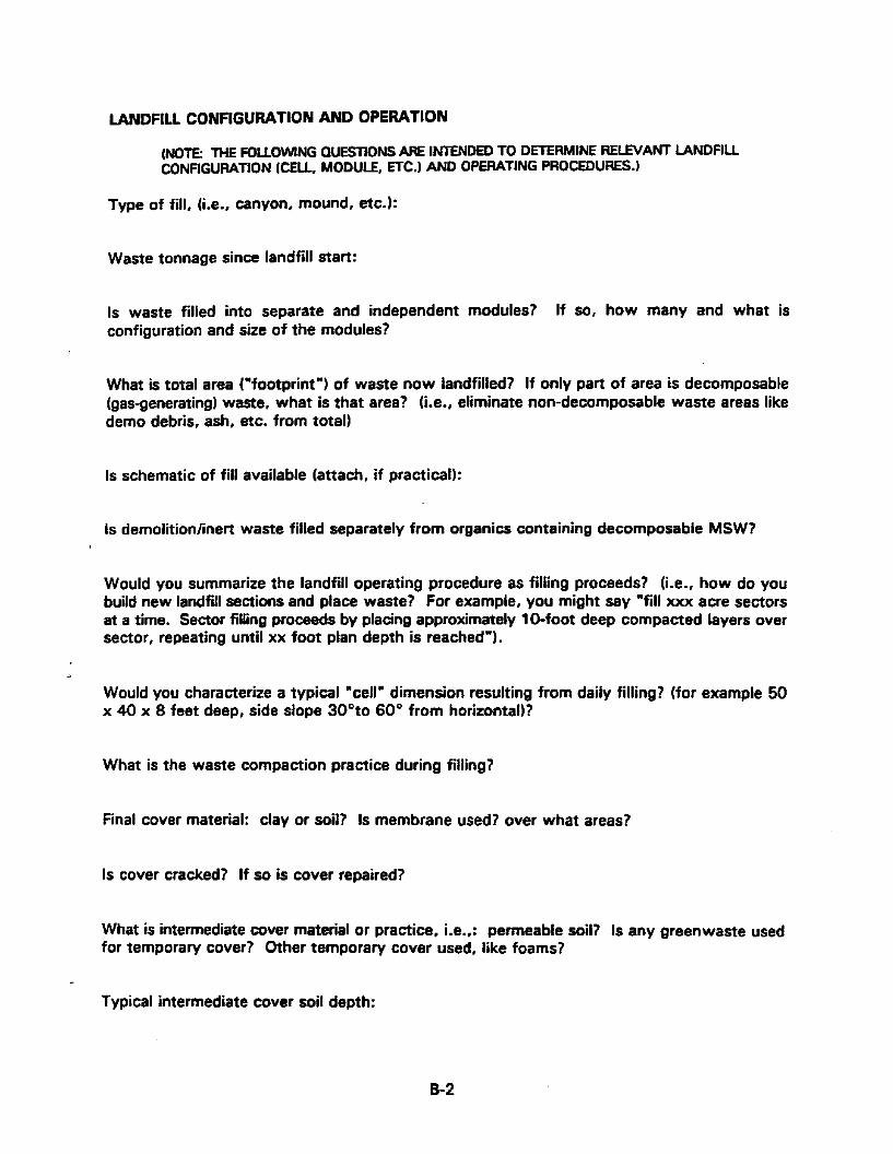
LANDFILL CONFIGURATION AND OPERATION

(NOTE: THE FOLLOWING QUESnONS ARE INTENDED TO DETERMINE RELEVANT LANDFILL CONFIGURAIION (CEU, MODULE, ETC.) AND OPERATING PROCEDURES.)

Type of fill, {Le., canyon, mound, etc.):

Waste tonnage since landfill start:

Is waste filled into separate and independent modules? configuration and size of the modules?

If so, how many and what is

What is total area ("footprint") of waste now iandfilled? If only part of area is decomposable (gas-generating) waste, what is that area? (Le., eliminate non-decomposable waste areas like demo debris, ash, etc. from total)

Is schematic of fill available (attach, if practical):

Is demolitionfinert waste filied separately from organics containing decomposable MSW?

Would you summarize the landfill operating procedure as filling proceeds? ke., how do you build new landfill sections and ptace waste? For example, you might say "fill xxx acre sectors at a time. Sector filling proceeds by placing approximately 10-foot deep compacted layers over sector, repeating until xx foot plan depth is reached").

Would you characterize a typical "cell" dimension resulting from daily filling? (for example 50 x 40 x 8 feet deep, side slope 30"to 60" from horizontal)?

What is the waste compaction practice during filling?

Final cover material: clay or soil? Is membrane used? over what areas?

Is cover cracked? If so is cover repaired?

What is intermediate cover material or practice, i-e.,: permeable soil? Is any greenwaste used for temporary cover? Other temporary cover used, like foams?

Typical intermediate cover soil depth:

B-2

(optional) Is the cover soit calcareous, that is containing limestone?

Has cover approach changed over past years? how?

WASTE COMPOSTION CHARACTERIZATION

(NOTE: THE PURPOSE OF THE FOUOWNG QUESTIONS IS TO GENEWUY DmRMINE THE PERCENTAGE AND TYPE OF DECOMPOSABLE WASTE THAT IS LANDFlLLED. RELEVANT INFOflMATION ALSO REQUESTED AND IS TO.BE SUPPLIED IN TABLE 1 .I

Can you estimate (from areas served) or otherwise characterize the percentaoes Landfilled of (a) incoming waste that is "normal" household- paper and putrescibles like food and yard wastes a n d everything else. (b) percentage that is business/o ffice/comme r cial- prin ci pall y paper and including putrescibles such as grocery and restaurant wastes, and (c) inert non- decomposables-these include wood, demolition debris like asphalt, ash, inett non- decomposable manufacturing wastes of various sorts.

Has any waste characterization been performed, i.e., % paper, food, plastic, metal, inerts?

Are there any "atypical" wastes--for example these could be large amounts of food processing or grocery wastes, paper mill and sewage sludges?

Are there significant "unusual" wastes-such as food processing plant wastes, decomposable byproducts of industrial processes, etc.?

Is there baling of waste? Is any waste shredding practiced? Are plastic bags and containers opened before placement? (This does not count compaction.) If so, specify.

Are there significant hazardous wastes (filled in past or components possibly seen in gas from older sectors)?

Is yard waste separated and composted? ,

What materials are recovered at landfill? For example:

APP" lances Tramp iron (cans), metals

WASTE MOISTURE ESTIMATION

Tires Cardboard

Paper Other

{NOTE: THE PURPOSE OF THE FOUOWNG QUESTIONS IS TO DETERMINE THE LIKELY MOISTURE CONTENT AND INFllTRATlON AT STE-VVHEN AND WHAT AMOUNT OF WASTE INFLUENCED, AND DEGREE OF SATURATION.)

B-3

Do you have moisture data on waste in the landfill? Or, what is moisture addition history at landfill-for example flooding or run-on events, liquid additions by waste type?

Is the cover material porous, allowing precipitation infittration, or clay (and shedding most precipitation)?

Is waste saturated in any part of landfill (indicated by liquid at base of wells, etc.)

Is leachate generated? If so how much and from where?

ts leachate recycled? .

Leachate characteristics:

leachate pH 7

other characteristics ke., alkalinity, nutrients) if known.

GAS RECOVERY DATA

(THE PURPOSE OF QUESTIONS BELOW IS TO CHARACTERIZE GAS RECOVERY M m O D S AND FLOW AND COMPOSITION MEASUREMENTS)

Are you supplying an energy system? If so, is the energy system gas Iimited? And, are you trying to maximize recovery for it?

Recovery system characteristics

Vertical well? If so,

Ratio of well depth/waste depth / Slotline or perforation extent: from - depth to ( above bottom)

Is layout triangular, square, or mix (irregular)

Ratio of well perforation depth to well separation

Trench?

Trench depth/was?e depth Trench depthhrench separation Length of typical trenches

Membrane cover present?

What is methane measurement method?

a Infrared absorption (landtech') meter? 0

8

Thermal conductivity (Gastech' or MSA' meter? Gas chromatograph (model/rnake if possible)?

Do you measure oxygen or nitrogen at all?

What is the flow measurement method? (Pitot tube, orifice meter, hot-wire anemometer, other)

Is recovery system tuned for maximum recovew? (i.e.88 throttle wells .below 50% concentration, increase flow from wells over 50% concentration, etc.)

If system is tuned, what is the methane "set point", i.e., concentration goal on adjustment? (-1 % Methane normally observed? [-)% Time interval between adjustments?

Is surface scan performed for methane concentration? If so, concentration criterion fur control (for example: added control needed if scan shows over 1000 ppm as methane)

Are any other criteria used for extraction adjustment, Le., surface pressure drop?

Is welling of decomposable waste total bee., all wetled within 3-5 years from waste placement) or partial? If partial, can you estimate the fraction of decomposable waste that is welled three or more years after placement?

Wellhead gas temperature: What are values if you have them and, do these vary from new to old sectors of the landfill?

(NOTE: PEASE FILL OUT TABLE 1 THE MORE ACCURATE THE INFORMATION YOU PROVIDE, THE BETTER.)

TABLE 1

WASTE PLACEMENT AND GAS RECOVERY DATA FOR LANDFILL (see explanations and instructions)

DESCRIPTION OF LANDFILL SECTOR (IF APPLICABLE) or, N. A. (check here)

C0rnpo6tt, tecycl, inert adjustm. 888

Annual Methsne Generation -

Comments on dsts/calc8

note pageIs1 Ski01

(U68 bt8r

I * Attach data for earlier yeers if relevant

B-6

-- NOTESEXPUNATIONS TO TABLE 1.

1 If you can do so, please provide the gate Waste tonnage receipts, in terms of total gate waste tons for each year. (for example: 500 tomlday x 300 open per year would be 150,000 tons.) We want to base the model on Y~IIY gate tonnag= since t h i ~ information landfill operators are most likely to have.

2. We want to adjust so that the basis for gas genetation is pnbl tonnage of 'typicaf' municipal waste whose decomposable organics are actually buried in the landfill, and from which gas is being extracted. 2 be nee&& From gate tonnage figures that you report, would you please designate and quantify 83 Well as possible any of the tonnage of

(a) Gate decomposable waste that is and other greenwaste, food, paper.

filled but instead composted, including yard waste

(b) Gate decomposable waste tonnage that is filled but recycled-paper, cardboard.

0 Repott estimated tonnage for stypically large amounts of inert waste-for example amounts of demolition waste over 20% of the total tonnage received, asphatt and concrete discards, etc. Please count wood waste as inert.

(d) Report as well, waste tonnaoe filled but not yet welled (in the next column provided).

NOTE: ltems a and b above-food and paper diverted after the gate (such as for recycling or composting) are especially important. These materials are normally the source of a major part of landfill gas. Their diversions (from filling) represent loss of gas generation potential. If you don't have exact numbers for various materials, provide estimates if you think they are reasonably accurate, and just note these as estimates ('est.').

You do rn have to acfpst for ghss, metal, or normal demo debris (even if demo debris is placed separately, or some glass or metal are recycled) since these are normally present in 'typical' waste that all landfills receive. "Normal" demo debris is up to 15% of waste weight

3. After the adjustments this value should be the gate waste tonnage with remaining decomposables actually landfilled within the year.

4. This figure should be based on the maximum sustainable gas recovery rate you observe (over a month or more in the year) with the gas system working optimally. If there is winter to summer variation you can average and note that. You can report gas recovery rates in your own units (cfm, etc.) and percentage methane and we will work out the rest. We can discuss.

5. Put any comments you think appropriate about waste placement or methane or other data here- just for example "percent methane varied between 45055%" or ' 15% of gas wells down all year" or anything else you think might affect accuracy. Use note section following for longer notes.

There are likely to be questions in many cases. Please cat1 Don Augenstein at 415-856-2850 or Greg Vogt at SCS Engineers, (703) 471-6150. We can also discuss in interviews. Thanks for your help.

APPENDIX C

METHANE GAS RECOVERY PROGRAM VERSION 1.1

Example Program Input Forms and Outputs

a Program Disk

c- 1

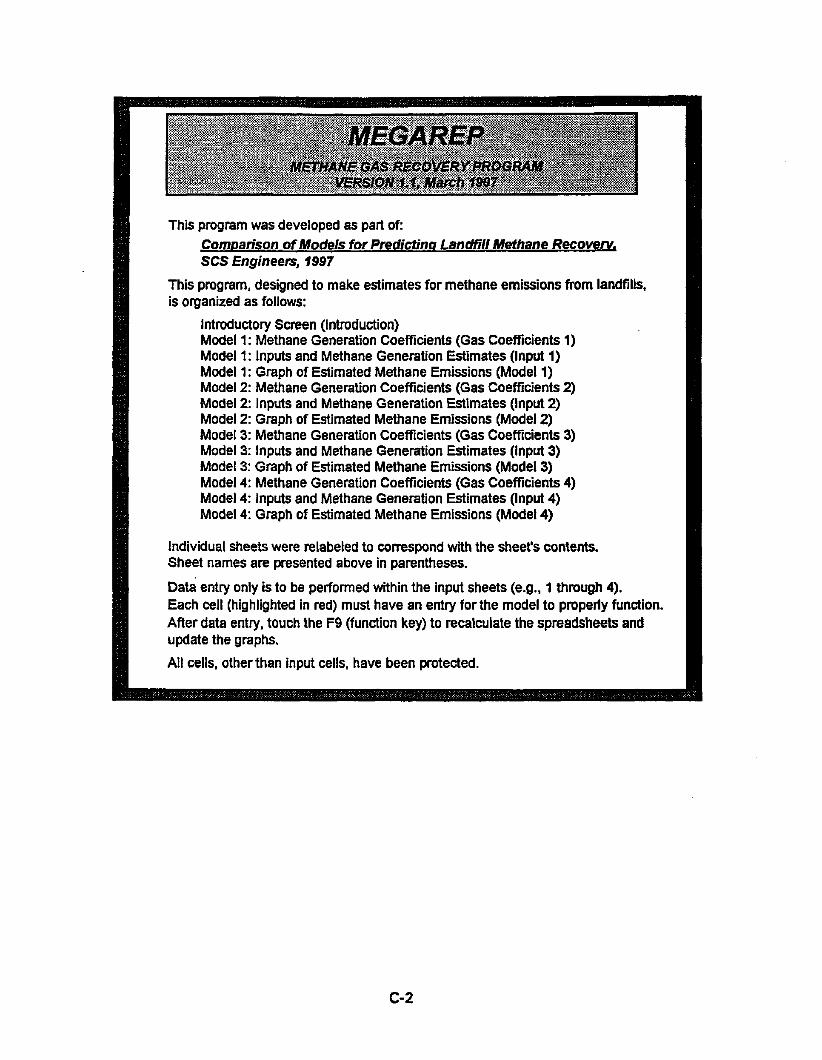
This program was developed as part of: ComDarison of Models for PrediCtina LandWl Methane Recoverv, SCS Engineers, f937

This program, designed to make estimates for methane emissions from landfills, is organized as follows:

Introductory Screen (Introduction) Model I: Methane Generation Coefficients (Gas Coefficients 1) Model 1: Inputs and Methane Generation Estimates (Input 1) Model I: Graph of Estimated Methane Emissions (Model 1) Model 2: Methane Generation Coefficients (Gas Coefficients 2) Model 2: Inputs and Methane Generation Estimates (Input 2) Modet 2: Graph of Estimated Methane Emissions (Model 2) Model 3: Methane Generation Coefficients (Gas Coefficients 3) Model 3: Inputs and Methane Generation Estimates (Input 3) Model 3: Graph of Estimated Methane Emissions (Model 3) Model 4: Methane Generation Coefficients (Gas Coefficients 4) Model 4: tnputs and Methane Generation Estimates (Input 4) Model 4: Graph of Estimated Methane Emissions (Model 4)

Individual sheets were relabeled to correspond with the sheet's contents. Sheet names are presented above in parentheses.

Data entry only is to be performed within the input sheets (e.g., 1 through 4). Each cell (highlighted in red) must have an entry for the model to properly function. After data entry, touch the F9 (fundion key) to recalculate the spreadsheets and update the graphs.

AH cells, other than input cells, have been protected.

c-2

ABC LANDFILL

Model I: Parameters Zero Order

~~ ~

Start Year NO. 0 End Year No. 20 Lo: 1,600 cubic feet Methanehon refuse

Lag time between placement and start of generation is assumed to be zero.

Methane Generation

Annual Refuse

Year (Tons)

Methane

(Million cubic feet 1 year) Generation .

1988 1989 1990 1991 1992 1993 1994 7 995 1996 1997 1998 1999 2000 2001 2002 2003 2004 2005 2006 2007 2008 2009 201 0

24,000 25,000 27,000 74,000 72,000 74,000 77,000 82,000 82,000 88,000 94,000 99,000

105,OOO 109,000 108,000 100,000 100,000 69,000 63,000 62,000 60,000

0 0

2 4 6

12 18 24 30 36 43 50 .

58 65 74 83 91 99

107 113 118 123 126 124 121

c-3

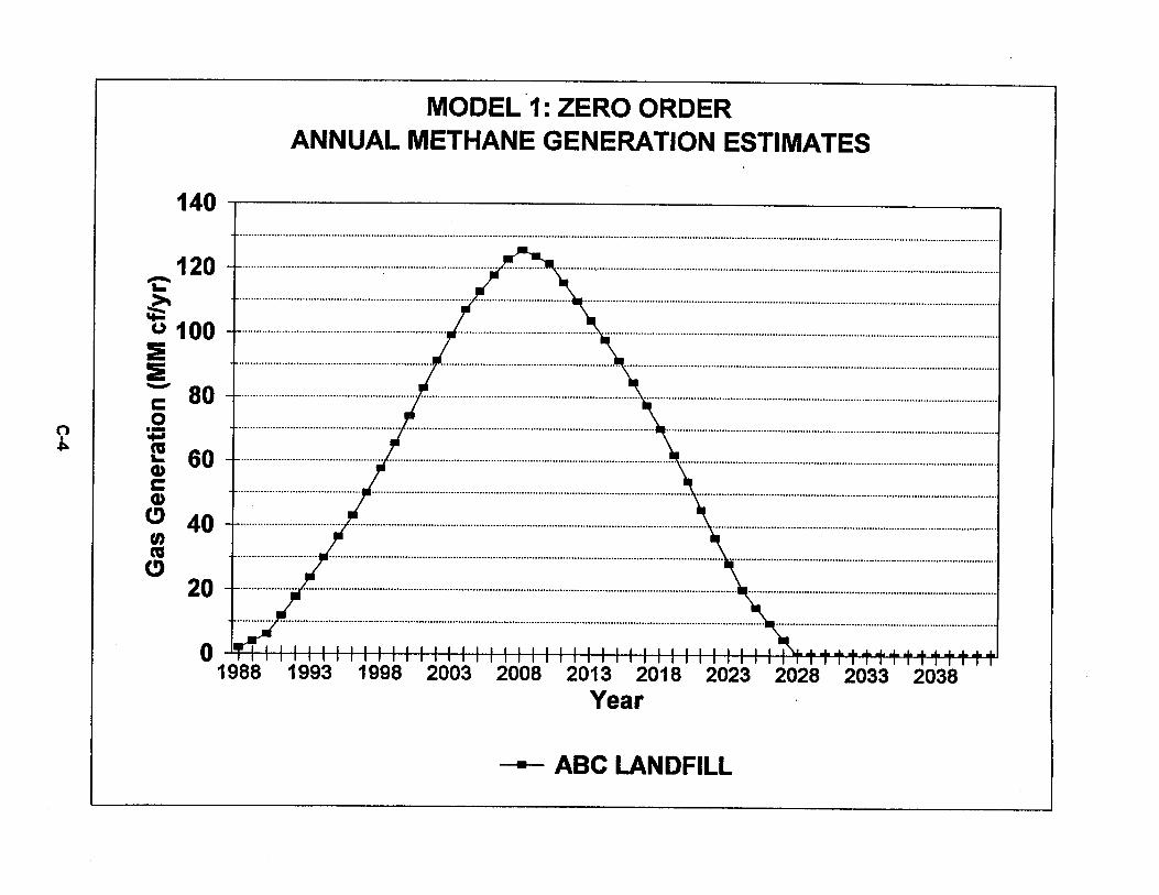
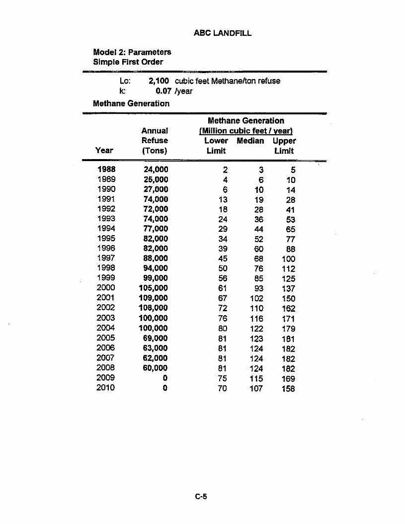
ABC LANDFILL

Model 2: Parameters Simple First Order

Lo: 2,'lOO cubic feet Methanelton refuse k: 0.07 /year

Methane Generation

Methane Generation Annual jMillion cubic feet I vear) Refuse Lower Median Upper

Year (Tons) Limit Limit

1988 1989 1990 I991 1992 1993 1994 1995 t 996 1997 1998 1999 2000 2001 2002 2003 2004 2005 2006 2007 2008 2009 201 0

24,000 25,000 27,000 74,000 72,000 74,000 77,000 82,000 82,000 88,000 94,000 99,000

~05,000 109,000 108,000 100,000 100,000 69,000 63,000 62,000 60,000

0 0

2 4 6

13 18 24 29 34 39 45 50 56 61 67 72 76 80 81 81 81 81 75 70

3 6

10 19 28 36 44 52 60 68 76 85 93

1 02 110 116 122 123 124 7 24 124 115 1 07

5 10 14 28 41 53 65 77 88

100 112 125 1 37 150 162 171 179 181 f 82 182 1 82 169 158

c-5

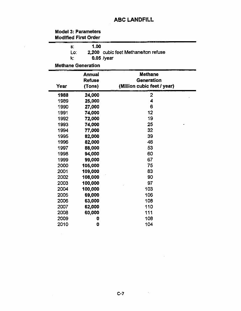
ABC LANDFILL

Model 3: Parameters Modified First Order

S: I .oo Lo: 2,200 cubic feet Methanelton refuse k: 0.05 lyear

Methane Generation

Annual Methane Refuse Generation

Year (Tons) (Million cubic feet I year) 1988 1989 1990 1991 1992 1993 1994 1995 1996 1997 1998 I999 2000 2001 2002 2003 2004 2005 2006 2007 2008 2009 201 0

24,000 25,000 27,000 74,000 72,000 74,000 77,000 82,000 82,000 88,000 94,000 99,000

105,000 109,000 108,000 ~00,QOO 100,000 69,000 63,000 62,000 60,000

0 0

2 4 6

12 19 25 32 39 46 53 60 67 75 83 90 97

103 106 108 110 111 108 104

c-7

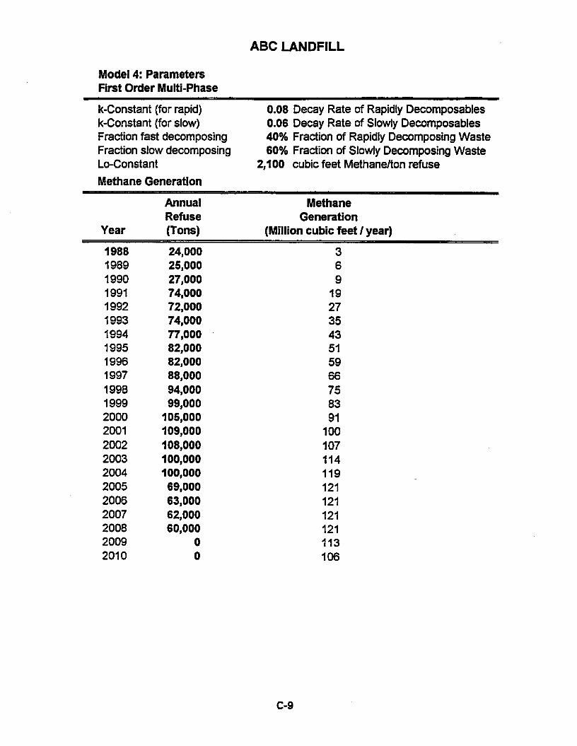
Model 4: Parameters First Order Multi-Phase

k-Constant (for rapid) 0.08 k-Constant (for slow) 0.06 Fraction fast decomposing 40% Fraction slow decomposing 60% to-con st ant 2,100 Methane Generation

Decay Rate of Rapidly Decomposables Decay Rate of Slowly Decomposables Fraction of Rapidly Decomposing Waste Fraction of Slowly Decomposing Waste cubic feet Methanehon refuse

Annual Methane Refuse Generation

Year (Tons) (Million cubic feet I year) 1988 1989 1990 1991 1992 1993 1994 1995 1996 1997 1998 I999 2000 2001 2002 2003 2004 2005 2006 2007 2008 2009 201 0

24,000 25,000 27,000 74,000 72,000 74,000 77,000 82,000 82,000 88,000 94,000 99,000

~05,000 109,000 108,OOO 100,000 100,000 69,000 63,000 62,000 60,000

0 0

3 6 9

19 27 35 43 51 59 66 75 83 91

100 107 314 119 121 121 121 121 113 106

c-9