Embed Size (px)
Citation preview
Report No 05/10
Crisis, Restructuring and Growth:
A Macroeconomic Perspective
by
Ingvild Almås
Gernot Doppelhofer
Jens Christian Haatvedt
Jan Tore Klovland
Krisztina Molnar
Øystein Thøgersen
SNF project no 1306
“Crisis, Restructuring and Growth”
CRISIS, RESTRUCTURING AND GROWTH
This report is one of a series of papers and reports published by the Institute for Research in
Economics and Business Administration (SNF) as part of its research programme “Crisis,
Restructuring and Growth”. The aim of the programme is to map the causes of the crisis and
the subsequent real economic downturn, and to identify and analyze the consequences for
restructuring needs and ability as well as the consequences for the long-term economic growth
in Norway and other western countries. The programme is part of a major initiative by the
NHH environment and is conducted in collaboration with the Norwegian Ministry of Trade
and Industry and the Research Council of Norway.
INSTITUTE FOR RESEARCH IN ECONOMICS AND BUSINESS ADMINISTRATION
BERGEN, APRIL 2010
ISSN 1503-2140
© Dette eksemplar er fremstilt etter avtale med KOPINOR, Stenergate 1, 0050 Oslo. Ytterligere eksemplarfremstilling uten avtale og i strid med åndsverkloven er straffbart og
kan medføre erstatningsansvar.
SNF Report 05/10
2
ISBN 978-82-491-0699-8 Printed Version
ISBN 978-82-491-0700-1 Electronic Version
ISSN 0803-4036
Contents Chapter 1: Macroeconomics Aspects of the Financial crisis – an Introduction ............................... 6
Corrections of financial imbalances .................................................................................................... 8
Short run gains – long run pains ........................................................................................................ 11
Stabilization policies .......................................................................................................................... 13
Macroeconomic prospects and ”de-coupling” .................................................................................. 15
Chapter 2: The financial crisis: Lessons from the interwar period .................................................. 18
Introduction ....................................................................................................................................... 18
The business cycle – chronology and severity: a comparison of the 1929-1933 cycle with the
present downturn ............................................................................................................................. 18
Financial market events: important similar features of the two cycles ............................................ 23
Asset markets ................................................................................................................................ 23
Money markets ............................................................................................................................. 27
Bank failures and banking legislation ............................................................................................ 29
The credit crunch ........................................................................................................................... 32
Monetary policy ............................................................................................................................ 35
The recovery phase: what are the lessons from the Great Contraction? ......................................... 36
What led out of the recession? ..................................................................................................... 37
Monetary policy in the aftermath of the recession – coping with changes in risk attitude,
liquidity preference and lending behavior of the banks .............................................................. 38
Financial crises and the economy of Norway in the interwar period ............................................... 40
The banking crises and their effects on business cycles and exchange rates ............................... 41
Bank behavior during and after the crisis ..................................................................................... 42
The choice of monetary regime and the international propagation of business cycle impulses . 42
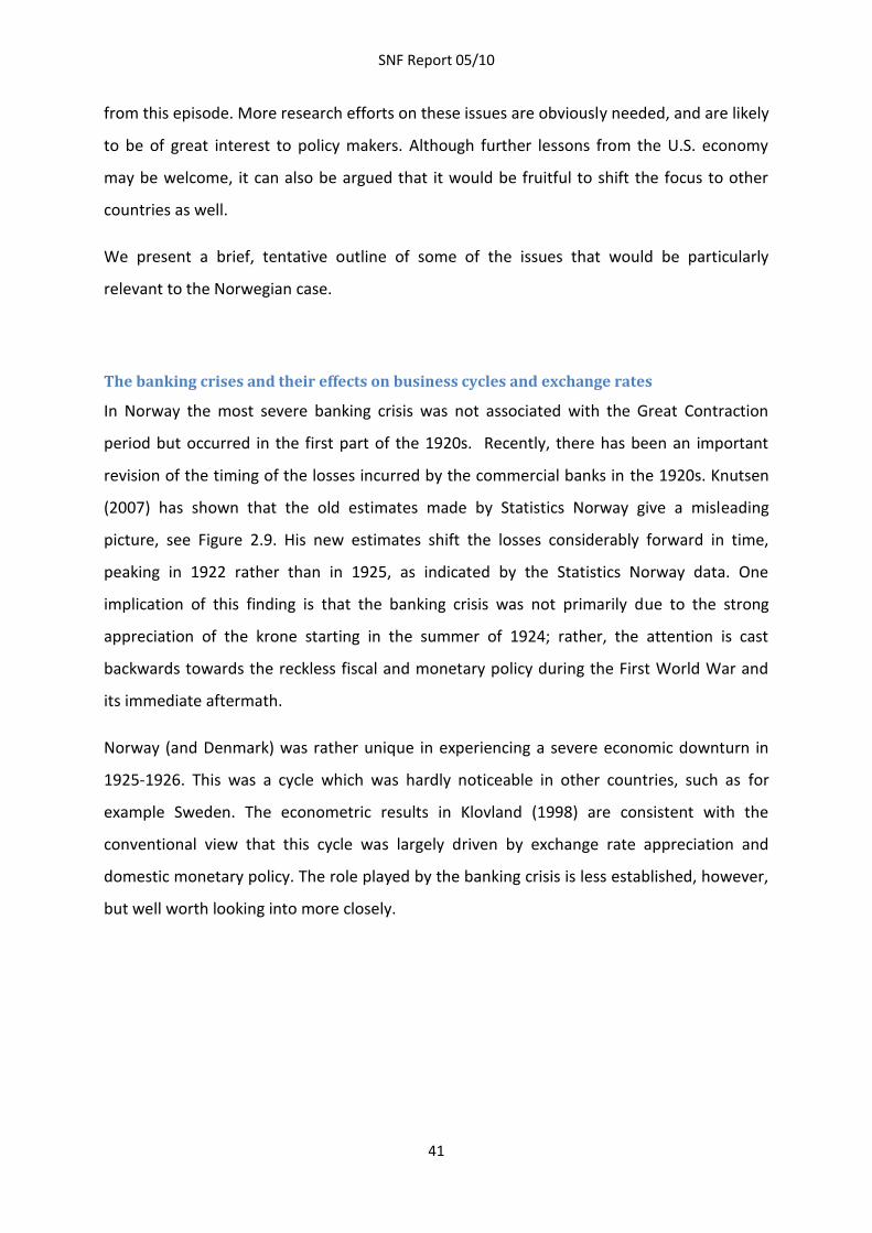
Financial crises and economic growth in the interwar years ........................................................ 43
Chapter 3: Determinants of Financial Crises ..................................................................................... 44
Typical financial crises ....................................................................................................................... 44
Banking Crises .................................................................................................................................... 47
Currency Crises .................................................................................................................................. 51
SNF Report 05/10
4
Twin Crises ......................................................................................................................................... 52
Debt Crises ......................................................................................................................................... 54
Aftermath of Financial Crises ............................................................................................................ 55
Nordic country experience ................................................................................................................ 58
Policy Lessons .................................................................................................................................... 60
Chapter 4: Financial Crises and Challenges for Monetary Policy .................................................... 61
Prelude to the financial crisis ............................................................................................................ 61
Developments on the financial market ......................................................................................... 62
Monetary policy before the crisis .................................................................................................. 63
Conventional monetary policy tools ................................................................................................. 64
Federal Funds Rate Target ............................................................................................................. 65
Discount Lending ........................................................................................................................... 65
Reserve Requirement .................................................................................................................... 66
The crises hits .................................................................................................................................... 66
Monetary policy during the crises ..................................................................................................... 68
Term Auction Facility ..................................................................................................................... 69
Providing international dollar liquidity .......................................................................................... 70
Term Securities Lending Facility .................................................................................................... 70
Bear Stearns .................................................................................................................................. 71
Primary Dealer Credit Facility ........................................................................................................ 72
After the failure of Lehman - the Fed’s new Alphabet soup ......................................................... 73
Conclusion ......................................................................................................................................... 74
Chapter 5: Adjustment of financial imbalances – China versus the United States ........................ 77
Chapter 6: Determinants of Financial Crises: Jointness and the Role of Expectations ................. 81
Chapter 7: Financial Frictions and Business Cycles ........................................................................... 82
Chapter 8: Sectoral allocation and endogenous political preferences ........................................... 86
References ............................................................................................................................................. 89
SNF Report 05/10
5
Part I: Macroeconomic Lessons and Policy Implications of Financial Crises
This report provides a broad presentation of research topics
related to the development of financial crises
SNF Report 05/10
6
Chapter 1: Macroeconomics Aspects of the Financial crisis – an Introduction
The global financial crisis of 2008 and 2009 has its background in both micro- and
macroeconomic developments. Too little and/or inefficient supervision of financial
institutions, myopic agents, herd behavior and a big dose of irrational exuberance have
interacted with macroeconomic features like global financial imbalances, the associated
global savings glut and lax monetary and fiscal policies in most parts of the world. Currently,
in the fourth quarter of 2009, the crisis has reached a stage where it is possible, with
reasonable precision, to describe its roots and causes. The depth and persistence of the
crisis are still uncertain, however. While the financial markets have been stabilized, and
seem in most segments to approach normalized functioning, the effects on the real economy
are still developing. So far, it is clear that the global business cycle is experiencing the
deepest and most persistent recession since the Second World War.
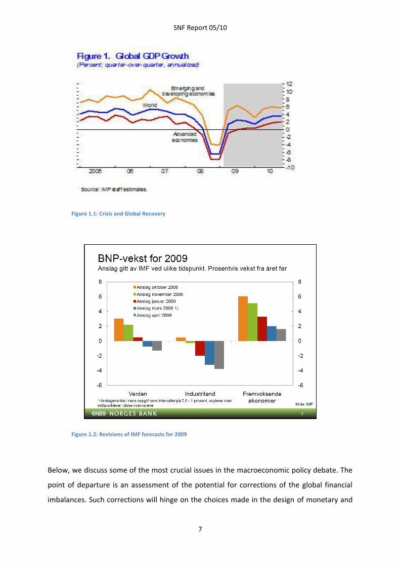
The dating of the business cycle trough remains uncertain, see Figures 1.1 and 1.2. Available
national account data (which include the second quarter of 2009) and the developments of
the range of more high-frequent macroeconomic indicators suggest that the global recession
bottomed out during the summer of 2009. The crucial question is whether the observed
macroeconomic “green shoots” reflect a robust rebound – or just more short-lived effects of
massive monetary and fiscal stimulations. Even more uncertain are the effects on the
underlying, long run trend growth (potential output). We conjecture that both the short run
business cycle dynamics as well as the effects on trend growth will vary significantly between
economies, depending on both the design of economic policies and other characteristics.
The challenges and trade-offs facing governments and central banks have hardly ever been
as complex as today.
SNF Report 05/10
7
Figure 1.1: Crisis and Global Recovery
Figure 1.2: Revisions of IMF forecasts for 2009
Below, we discuss some of the most crucial issues in the macroeconomic policy debate. The
point of departure is an assessment of the potential for corrections of the global financial
imbalances. Such corrections will hinge on the choices made in the design of monetary and
SNF Report 05/10
8
fiscal policy. For the time being, we observe extremely expansionary policies, providing relief
for the business cycle conditions, but partly offsetting the effects on the corrections of the
financial imbalances. This raises questions about the adverse long run effects of the short
run gains of stimulating aggregate demand.
Both the ability to stimulate aggregate demand and the long run effects will vary across
economies. The vulnerability of each single economy towards the global developments will
depend on characteristics such as industry structure and the initial anchoring of monetary
and fiscal policy strategies. A particularly interesting issue with respect to cross country
heterogeneity is the relationship between the established, industrialized countries and the
emerging markets, recall the discussion over the validity of the decoupling hypothesis.
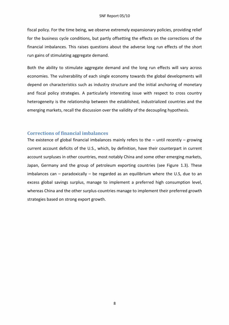
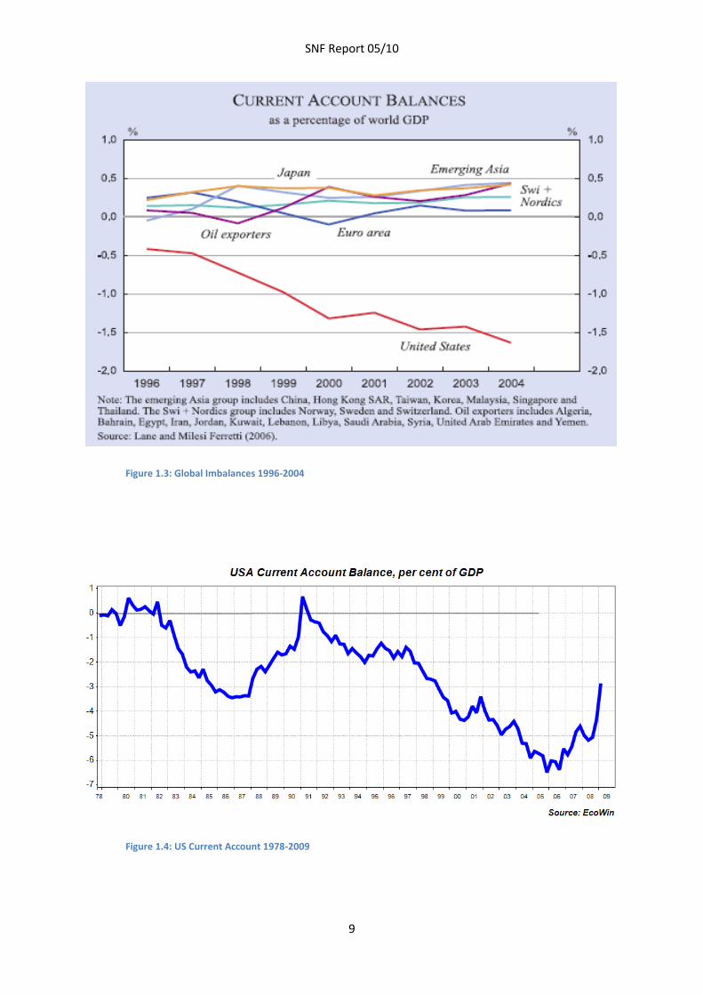
Corrections of financial imbalances
The existence of global financial imbalances mainly refers to the – until recently – growing
current account deficits of the U.S., which, by definition, have their counterpart in current
account surpluses in other countries, most notably China and some other emerging markets,
Japan, Germany and the group of petroleum exporting countries (see Figure 1.3). These
imbalances can – paradoxically – be regarded as an equilibrium where the U.S, due to an
excess global savings surplus, manage to implement a preferred high consumption level,
whereas China and the other surplus-countries manage to implement their preferred growth
strategies based on strong export growth.
SNF Report 05/10
9
Figure 1.3: Global Imbalances 1996-2004
Figure 1.4: US Current Account 1978-2009
SNF Report 05/10
10
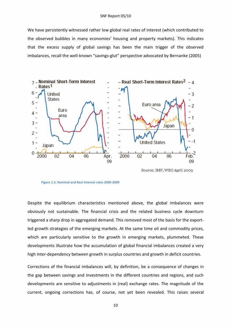
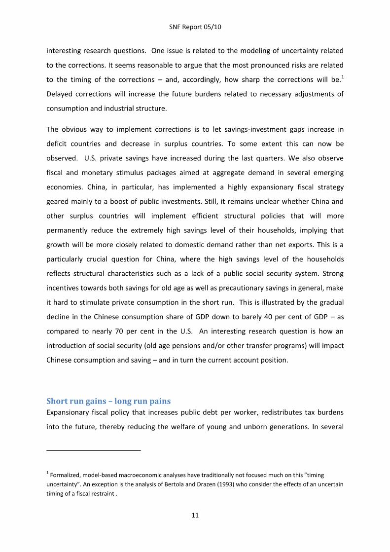
We have persistently witnessed rather low global real rates of interest (which contributed to
the observed bubbles in many economies’ housing and property markets). This indicates
that the excess supply of global savings has been the main trigger of the observed
imbalances, recall the well-known “savings-glut” perspective advocated by Bernanke (2005)
Figure 1.5: Nominal and Real Interest rates 2000-2009
Despite the equilibrium characteristics mentioned above, the global imbalances were
obviously not sustainable. The financial crisis and the related business cycle downturn
triggered a sharp drop in aggregated demand. This removed most of the basis for the export-
led growth strategies of the emerging markets. At the same time oil and commodity prices,
which are particularly sensitive to the growth in emerging markets, plummeted. These
developments illustrate how the accumulation of global financial imbalances created a very
high inter-dependency between growth in surplus countries and growth in deficit countries.
Corrections of the financial imbalances will, by definition, be a consequence of changes in
the gap between savings and investments in the different countries and regions, and such
developments are sensitive to adjustments in (real) exchange rates. The magnitude of the
current, ongoing corrections has, of course, not yet been revealed. This raises several
SNF Report 05/10
11
interesting research questions. One issue is related to the modeling of uncertainty related
to the corrections. It seems reasonable to argue that the most pronounced risks are related
to the timing of the corrections – and, accordingly, how sharp the corrections will be.1
Delayed corrections will increase the future burdens related to necessary adjustments of
consumption and industrial structure.
The obvious way to implement corrections is to let savings-investment gaps increase in
deficit countries and decrease in surplus countries. To some extent this can now be
observed. U.S. private savings have increased during the last quarters. We also observe
fiscal and monetary stimulus packages aimed at aggregate demand in several emerging
economies. China, in particular, has implemented a highly expansionary fiscal strategy
geared mainly to a boost of public investments. Still, it remains unclear whether China and
other surplus countries will implement efficient structural policies that will more
permanently reduce the extremely high savings level of their households, implying that
growth will be more closely related to domestic demand rather than net exports. This is a
particularly crucial question for China, where the high savings level of the households
reflects structural characteristics such as a lack of a public social security system. Strong
incentives towards both savings for old age as well as precautionary savings in general, make
it hard to stimulate private consumption in the short run. This is illustrated by the gradual
decline in the Chinese consumption share of GDP down to barely 40 per cent of GDP – as
compared to nearly 70 per cent in the U.S. An interesting research question is how an
introduction of social security (old age pensions and/or other transfer programs) will impact
Chinese consumption and saving – and in turn the current account position.
Short run gains – long run pains
Expansionary fiscal policy that increases public debt per worker, redistributes tax burdens
into the future, thereby reducing the welfare of young and unborn generations. In several
1 Formalized, model-based macroeconomic analyses have traditionally not focused much on this ”timing
uncertainty”. An exception is the analysis of Bertola and Drazen (1993) who consider the effects of an uncertain
timing of a fiscal restraint .
SNF Report 05/10
12
OECD economies where tax rates are already high at the outset, and ageing leads to
escalating fiscal changes in the years to come, this motivates social security reforms
intending to both reduce the magnitude of future pension expenditures and stimulate labor
supply and growth.
When economies with significant fiscal challenges currently run significant fiscal deficits,
future tax burdens increase to even higher levels. In deficit economies, like notably the US
and the UK, this implies that the room to maneuver for the potential implementation of new
welfare programs or other political projects declines, recall, as an example, the plans of the
Obama administration to present a major health care reform in the US.
These developments raise interesting research questions about fiscal policy trade-offs in the
years to come. Is it wise that economies, which have contributed to the current crises by
saving way too little, in effect attempt to offset the initiated corrections by fiscal policies
that increase the public debt? The objective of the implemented fiscal policies is exactly this,
namely to offset the effects of increased private saving in a way which keeps aggregated
domestic demand growth afloat.
The observed expansionary policy measures express, explicitly or implicitly, that the short
run business cycle problems and the related systemic problems in major segments of the
financial markets are assessed as extremely severe. Policy-makers may, for example, refer to
the fear of social tension and problems that might spin out of control if the unemployment
rates hit the highest levels since the great depression. Thus, the view of most policy-makers
seems to be that the long-run price of the huge keynesian stimulus packages is justified.
It is in any case relevant to assess the consequences of fiscal policies that counteract
intuitive, and, in the long run, unavoidable corrections of the global financial imbalances. It is
worth noting that aggressive fiscal policies that contribute to private consumption growth in
the US and other deficit-economies, may well be popular along several dimensions. They will
reduce the fall in China’s (and other surplus economies’) export, and will, of course, provide
short run stimulation of aggregate demand.
SNF Report 05/10
13
The issue is whether this will contribute to new – and potentially even bigger – future crises.
The analogy to US economic policy in 1998 is striking.2 In 1998 the US Central Bank, the
Federal Reserve, implemented a series of so-called ”emergency interest rate cuts” in order
to stimulate aggregate demand and provide relief to the financial markets in response to
external shocks including crises in Asia and Russia and financial market unease (recall the
collapse of the big hedge fund, LTCM). The expansionary policies were very successful in the
short run. Private consumption increased significantly. In turn, this paved the way for a
continued expansion of Asian exports, and consequently inflated the global imbalances. The
long run price of these policies was – as assessed from the current stage – high. The effects
include high private debt accumulation, housing bubbles, and a persistent global surplus-
supply of liquidity that acted as a catalyst for bad incentives and practices within many of the
worlds’ major financial institutions. An obvious issue is whether today’s tremendous
monetary and fiscal stimulus will cement the global financial imbalances and increase the
exposure to more asset price bubbles and boom-bust cycles in the real economy.
Stabilization policies
The financial crisis has triggered a big debate about the role and design of stabilization
policies, particularly the monetary policy framework and the conduct of interest rate setting.
The widespread (flexible) inflation targeting paradigm has received a lot of criticism, both in
economies with explicit inflation targets and in economies, like the US, with more implicit
inflation targets. A common argument is that interest rates were set at very low levels for
far too long, reflecting the fact that cheap imports from China and other emerging markets
contributed to low consumer price inflation everywhere. This was a main explanation for
asset price inflation and associated bubbles. Because asset price developments are generally
not reflected by the standard inflation indexes targeted by central banks, many observers
argue that these developments were more or less neglected by central banks in their
interest rate decisions.
2 See the op-ed piece of Stephen Roach, Chairman of Board in Morgan Stanley Asia, in Financial Times 10.03.09,
entitled ”Grow now, ask questions later – formula will end in tears”.
SNF Report 05/10
14
Former US central bank governor, Alan Greenspan, was well-known for his asymmetric view
on how central banks should react to asset prices.3 He argued that asset prices should not
influence interest rates during the boom-phase of an asset price cycle. However, the central
bank should come to the rescue, cutting interest rates aggressively when the asset price
bubble eventually burst. Naturally, this view, in its crude form, has been discredited during
the last couple of years.
Additional research questions are partly related to the effects and interpretation of credit
growth and asset prices within today’s ”best international practice” flexible inflation
targeting framework, and partly to the coordination between monetary policy and other
policy measures. The basic principle of flexible inflation targeting is that interest rates should
be set in order to obtain an optimal trade-off between the prospects for inflation (i.e. the
expected path of actual inflation vs. the inflation target) and the prospects for real economic
activity, typically specified as the expected developments of the output gap (i.e. the
expected path of actual output vs. the estimated trend output). According to the consensus
view over the last decades, asset prices are valuable indicators for these objective variables.
It is also widely accepted that asset price movements (particularly sharp drops associated
with the burst of bubbles) impact future output gaps. A relevant question is whether central
banks throughout the world underestimated the strength of the link between asset prices
and other key variables, a link that might be highly non-linear for sharp drops in asset prices.
Before the focus is directed to potential reforms of the inflation targeting paradigm per se,
attention should be directed to central banks’ modeling of the transmission mechanism
related to the interaction between asset prices, interest rates and other key variables.
The observed magnitude of the global recession caused by the financial crises, and the
evidence provided by Reinhart and Rogoff (2009a) , which shows that recessions associated
with asset price bubbles and banking crises are particularly deep and prolonged, does also
call for attention towards other policy measures than monetary policy alone. This obviously
includes macro-prudential policies. A main issue is better supervision and regulation of the
3 See Blinder and Reis (2005).
SNF Report 05/10
15
banking sector in order to avoid the observed strong tendency in many countries to a pro-
cyclical lending practice due to the flawed design of banks’ capital requirements.
Macroeconomic prospects and ”de-coupling”
The global recession of 2008 – 2009 has been highly synchronized between countries and
regions. This is, intuitively, consistent with a severe drop in global trade. The depth of the
recession, its persistence, and, particularly, the prospects for the structural, long run trend
growth, are likely to vary widely, however.
Long run variations in the trend growth of an economy are well known. The US, for example,
experienced a trend real growth rate close to 3.5 per cent annually during the period from
1950 to the beginning of the 1970s. Then the trend growth rate decreased to approximately
2.5 per cent for the next two decades, until it again increased during the last part of the
1990s. An important issue is whether a return to an anemic trend growth trajectory is likely
in the same way as in the early 1970s. Potential triggers include:
Escalation of protectionistic measures: The observed drop in world trade is so far – to
a first approximation – fully caused by the drop in aggregate demand associated with
the downturn of the business cycle. This effect is temporary. We have, however,
witnessed a number of suggested, and to a minor extent implemented, policy
measures with protectionistic elements. This includes the transfers to the US car
industry and Chinese tax and tariff policies supporting China’s own export industry.
At the current stage, the risks of devastating trade wars and big scale protectionism
seem small, however.
Credit rationing: A main ingredient of the financial crisis is the malfunctioning of the
banking sector. While the many significant measures implemented by central banks
and other authorities have clearly stabilized the situation in most economies, in
several countries it is still not the case that the working of the banking sector and the
financial markets is normalized. This implies that there is a risk of a prolonged period
with credit rationing in such countries, particularly hurting investments, and,
ultimately, growth.
SNF Report 05/10
16
Higher and/or more volatile inflation, stagflation: We have witnessed aggressive
monetary policies in most economies, pushing key interest rates down to very low
levels and including various types of quantitative easening on a grand scale. This has
contributed to a sharp increase in money supply. As a consequence, inflation
expectations have increased and much attention is now directed to the risk of higher
inflation over, say, a two to five year horizon. In particular deficit countries where
deleveraging and higher tax burdens put a drag on private demand may face a
stagflationary climate.
Regulation and efficiency: The financial crisis is a crisis of the market-based economic
system. Not surprisingly, the political debate now focuses on the potential
implementation of stricter regulations and closer supervision of many financial
institutions. The design, scale and efficiency effects of the innovations in this area
may well impact trend growth.
While the issues discussed above are important for the global economy as a whole, there are
also a series of more idiosyncratic issues which are crucial for individual countries. These
include: the individual economy’s dependency on trade; the characteristics of the export
sector, i.e. the type and income elasticity of the export products; the terms of trade
implications; the initial anchoring of the individual economy’s monetary and fiscal policy
strategies; the initial situation with respect to foreign financial assets, current account
balance, public debt and budget balance.
A highly interesting issue is the relationship between the industrialized economies and the
emerging market economies. During the last decades, significant and fairly persistent
differences in growth and also financial market performance suggested the “decoupling
hypothesis”. In its simplest (and maybe naive) form, decoupling was interpreted to imply
that the growth rates of China and other emerging markets were immune against declining
growth in the US and other industrialized countries. The developments over the last couple
of years clearly show that this interpretation of decoupling was false, see the discussion
above regarding the interdependency caused by global financial imbalances.
SNF Report 05/10
17
The lack of support to the simplest form of the decoupling hypothesis does not, however,
rule out the existence of significant differences in growth dynamics. The main underlying
drivers for strong growth in China and several other emerging markets are urbanization,
industrialization and human capital accumulation. These mechanisms are intact despite the
business cycle downturn we have witnessed. Thus, the growth prospects for the emerging
markets and the interdependence between these countries and the established
industrialized economies are center-stage for the understanding of the global economic
prospects.
SNF Report 05/10
18
Chapter 2: The financial crisis: Lessons from the interwar period
Introduction
We develop three major themes in this chapter: (A) What can we learn from the Great
Depression of 1929-1933 in the United States with respect to the causes of the cyclical
downturn and the behavior of the economy during the contraction phase of the cycle? (b)
Does the historical experience during the recovery phase, i.e. from 1933 onwards, present
any lessons that are relevant for today’s policy response? (C) How did financial crises in
Norway during the interwar period affect the behavior of the real economy in terms of
business cycles and economic growth?
In the first two sections the focus is thus on the interaction between monetary policy, the
financial sector and real output in the United States, mainly in the 1930s. In the third section
the focus is shifted towards Norway – trying to understand how Norway differed from other
countries, particularly the United States. Here the time period from which our policy lessons
are extracted is extended to the whole interwar period.
The business cycle – chronology and severity: a comparison of the 1929-1933 cycle with the present downturn The Great Depression (or Contraction, as it is sometimes called) – the business cycle
depression starting in August 1929, and lasting until March 1933 - was the longest and by
far the most severe of all business cycles ever recorded in the United States.4 In terms of
business cycle history this cycle occupies a unique role. As the present financial crisis
developed into a major economic contraction period the Great Depression was used as a
benchmark of a ‘worst case scenario’.
4 The authoritative business cycle chronology of the United States, originally developed by Burns and Mitchell
(1946) and maintained by the National Bureau of Economic Research, goes back to 1854. The list is available at
http://www.nber.org/cycles/cyclesmain.html.
SNF Report 05/10
19
A useful summary measure of the severity of business cycles is the concept of output loss as
defined by Christina Romer (1994). Looking at the graph of a time series representing the
business cycle during a contraction period, a horizontal line can be drawn from the most
recent peak of the business cycle (point A). When the economy is starting to recover again
the line will intersect the data series at a point B when the previous peak level of output has
been reached once again. The output loss is then measured as the area below the waterline
and the bottom of the lake as defined by the time series, typically represented by industrial
production or similar series. This measure thus comprises two important aspects of a cycle:
its duration and its depth.
Using this measure it turns out that the 1929-1933 cycle is 4.7 times as bad as the next worst
cycle, the famous restocking cycle in the immediate aftermath of World War I, which was a
short but particularly steep cycle during 1919-1921. It also turns out that the top three cycles
in terms of severity on this list all belong to the interwar period. The third cycle was a less
spectacular, but quite severe, downturn in the United States in 1937.
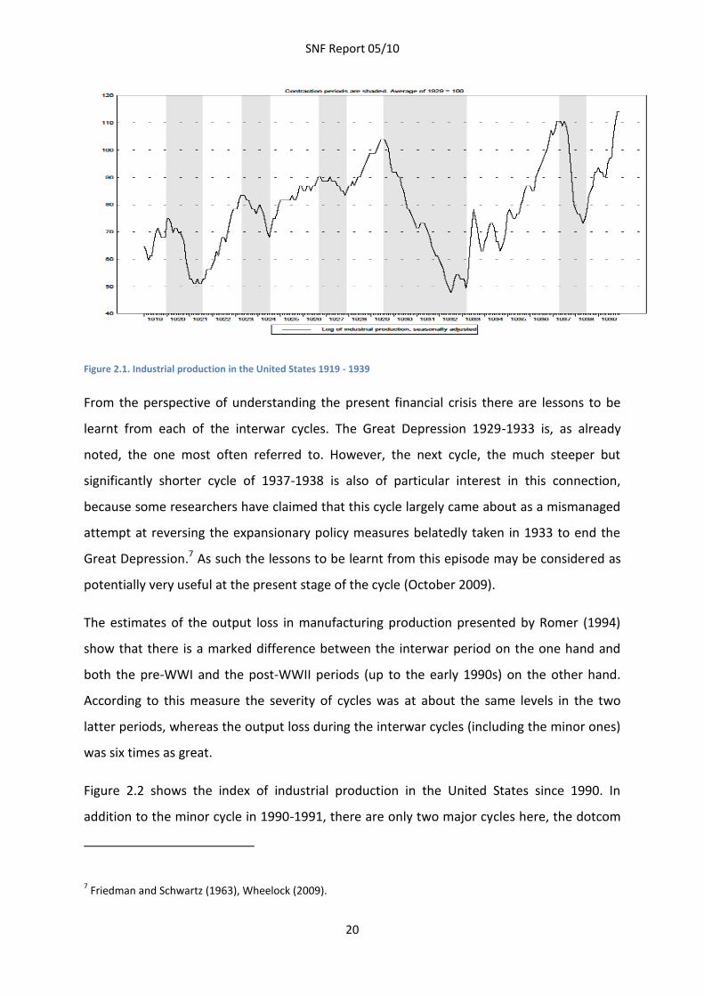
Figure 2.1 graphs the level of the industrial production index in the interwar period, with the
contraction periods, as defined by the National Bureau of Economic Research (NBER), being
shaded.5 The three major recessions stand out clearly in this graph. There were, in addition,
two minor cycles, in 1923-1924 and in 1926-1927.6
5 Because the NBER looks at several business cycle indicators in addition to industrial output the peaks and
troughs shown in the graph will not always coincide exactly with those of output.
6 The data on industrial production are taken from the database of the Federal Reserve Bank of St Louis (FRED),
available at http://research.stlouisfed.org/fred2/.
SNF Report 05/10
20
Figure 2.1. Industrial production in the United States 1919 - 1939
From the perspective of understanding the present financial crisis there are lessons to be
learnt from each of the interwar cycles. The Great Depression 1929-1933 is, as already
noted, the one most often referred to. However, the next cycle, the much steeper but
significantly shorter cycle of 1937-1938 is also of particular interest in this connection,
because some researchers have claimed that this cycle largely came about as a mismanaged
attempt at reversing the expansionary policy measures belatedly taken in 1933 to end the
Great Depression.7 As such the lessons to be learnt from this episode may be considered as
potentially very useful at the present stage of the cycle (October 2009).
The estimates of the output loss in manufacturing production presented by Romer (1994)
show that there is a marked difference between the interwar period on the one hand and
both the pre-WWI and the post-WWII periods (up to the early 1990s) on the other hand.
According to this measure the severity of cycles was at about the same levels in the two
latter periods, whereas the output loss during the interwar cycles (including the minor ones)
was six times as great.
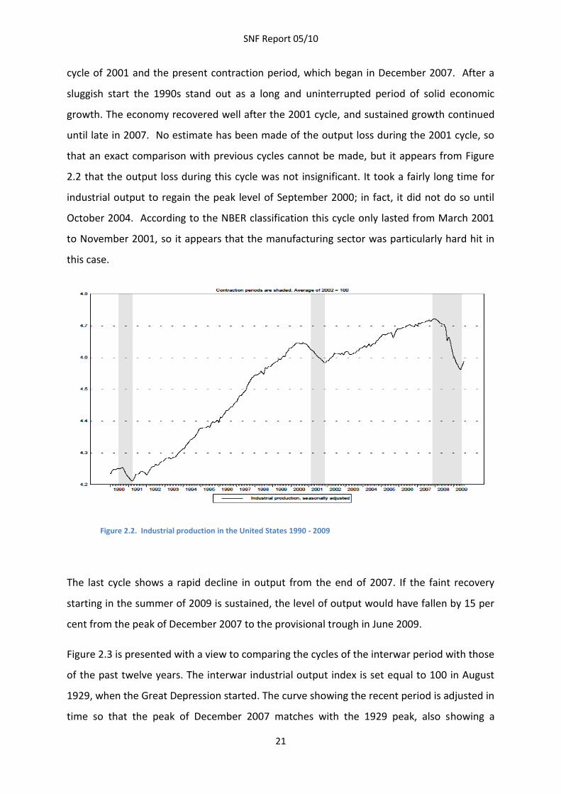
Figure 2.2 shows the index of industrial production in the United States since 1990. In
addition to the minor cycle in 1990-1991, there are only two major cycles here, the dotcom
7 Friedman and Schwartz (1963), Wheelock (2009).
SNF Report 05/10
21
cycle of 2001 and the present contraction period, which began in December 2007. After a
sluggish start the 1990s stand out as a long and uninterrupted period of solid economic
growth. The economy recovered well after the 2001 cycle, and sustained growth continued
until late in 2007. No estimate has been made of the output loss during the 2001 cycle, so
that an exact comparison with previous cycles cannot be made, but it appears from Figure
2.2 that the output loss during this cycle was not insignificant. It took a fairly long time for
industrial output to regain the peak level of September 2000; in fact, it did not do so until
October 2004. According to the NBER classification this cycle only lasted from March 2001
to November 2001, so it appears that the manufacturing sector was particularly hard hit in
this case.
Figure 2.2. Industrial production in the United States 1990 - 2009
The last cycle shows a rapid decline in output from the end of 2007. If the faint recovery
starting in the summer of 2009 is sustained, the level of output would have fallen by 15 per
cent from the peak of December 2007 to the provisional trough in June 2009.
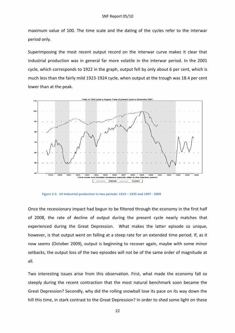
Figure 2.3 is presented with a view to comparing the cycles of the interwar period with those
of the past twelve years. The interwar industrial output index is set equal to 100 in August
1929, when the Great Depression started. The curve showing the recent period is adjusted in
time so that the peak of December 2007 matches with the 1929 peak, also showing a
SNF Report 05/10
22
maximum value of 100. The time scale and the dating of the cycles refer to the interwar
period only.
Superimposing the most recent output record on the interwar curve makes it clear that
industrial production was in general far more volatile in the interwar period. In the 2001
cycle, which corresponds to 1922 in the graph, output fell by only about 6 per cent, which is
much less than the fairly mild 1923-1924 cycle, when output at the trough was 18.4 per cent
lower than at the peak.
Figure 2.3. US Industrial production in two periods: 1919 – 1935 and 1997 - 2009
Once the recessionary impact had begun to be filtered through the economy in the first half
of 2008, the rate of decline of output during the present cycle nearly matches that
experienced during the Great Depression. What makes the latter episode so unique,
however, is that output went on falling at a steep rate for an extended time period. If, as it
now seems (October 2009), output is beginning to recover again, maybe with some minor
setbacks, the output loss of the two episodes will not be of the same order of magnitude at
all.
Two interesting issues arise from this observation. First, what made the economy fall so
steeply during the recent contraction that the most natural benchmark soon became the
Great Depression? Secondly, why did the rolling snowball lose its pace on its way down the
hill this time, in stark contrast to the Great Depression? In order to shed some light on these
SNF Report 05/10
23
issues we need to focus on some features that were similar and some that were quite
different in the two episodes. The focus will mainly be on financial market conditions and
monetary policy. Many other factors, such as fiscal policy, social policy, labor market
institutions and demographic trends, are obviously of relevance as well in this connection,
but a discussion of these are beyond the scope of the present chapter.
Financial market events: important similar features of the two cycles
We present some brief comparative remarks on the following aspects of the financial crises
now and then: (1) asset markets (2) money markets (3) bank failures and banking legislation
(4) the credit crunch (5) monetary policy.8
Asset markets
The housing market has played a key role in the present financial crisis. The sub-prime
market only collapsed after house prices started to fall late in 2006. This is widely believed to
be the spark that ignited the financial crisis. In contrast, falling house prices are not usually
cited as a prominent factor in the Great Depression in the United States. Taking a closer look
at the housing market in the 1920s, however, reveals that there was indeed a real estate
bubble in the 1920s, which burst in 1926.9 The consequences were less severe than in the
most recent crisis, but viewed together with the subsequent stock market crash, it
weakened the balance sheets of households and financial institutions prior to the turmoil of
the Great Depression. When the value of their mortgage debt increased significantly relative
to the market value of their tangible wealth, the financial fragility of households increased,
leaving them more vulnerable to even more severe financial shocks that were to come a few
years later.
8 Bordo and Haubrich (2009) review the role of credit crises as a cause of all business cycle contractions from
1875 to the present.
9 White (2009)
SNF Report 05/10
24
White (2009) presents some interesting arguments why house price bubbles create greater
dangers to financial stability now than in the 1920s. Ever since Roosevelt’s New Deal
measures to expand home ownership have been an important item on the political agenda.
Federal institutions like Fannie Mae and Freddie Mac have been set up with a view to
channeling mortgage loans to new groups of homeowners. This has drawn higher risk
families into the home buying market, which has led to increasing foreclosure rates in
turbulent periods. In addition, federal deposit insurance, financial innovations and more
liberal banking regulation have induced banks to take more risks. Because the banking
system is now more integrated than in the 1920s, locally generated shocks have the
potential of causing much more serious nationwide problems.
On the other hand, the behavior of financial markets exhibits some strikingly similar
features. The most well known feature of financial market behavior is the collapse of the
stock market in September 1929. Stock prices on the New York Stock Exchange, as
measured by the Dow Jones Industrial Average, fell continuously over a period of 34 months,
from September 1929 to July 1932. At the trough in July 1932 the value of the index was
only 10.8 per cent of the maximum that prevailed in September 1929. In the present crisis
the period of falling stock prices only extends to less than one and a half years, and the
lowest index value recorded is slightly less than 50 per cent of the peak value in October
2007. As we saw in the case of industrial output the basic similarity between the two
episodes lies with the speed of the initial fall (in output and stock prices); the crucial
difference is the length of the contraction period.
The security markets provide interesting material for a comparison between the two
episodes. In both cases we see a major deterioration in the financing conditions of private
business firms. The market prices of bonds issued by the corporate sector fell significantly, in
particular those with a low credit rating. This made it more costly to raise capital on the
security markets; in some cases this option became closed to borrowers. On the other hand,
the prices of government bills and bonds soared, bringing down the yield on such papers to
very low levels. These observations all reflect the general scramble for safety on the part of
the investors, often referred to as a flight to quality.
SNF Report 05/10
25
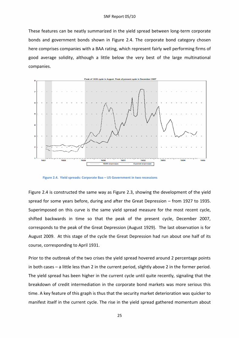
These features can be neatly summarized in the yield spread between long-term corporate
bonds and government bonds shown in Figure 2.4. The corporate bond category chosen
here comprises companies with a BAA rating, which represent fairly well performing firms of
good average solidity, although a little below the very best of the large multinational
companies.
Figure 2.4. Yield spreads: Corporate Baa – US Government in two recessions
Figure 2.4 is constructed the same way as Figure 2.3, showing the development of the yield
spread for some years before, during and after the Great Depression – from 1927 to 1935.
Superimposed on this curve is the same yield spread measure for the most recent cycle,
shifted backwards in time so that the peak of the present cycle, December 2007,
corresponds to the peak of the Great Depression (August 1929). The last observation is for
August 2009. At this stage of the cycle the Great Depression had run about one half of its
course, corresponding to April 1931.
Prior to the outbreak of the two crises the yield spread hovered around 2 percentage points
in both cases – a little less than 2 in the current period, slightly above 2 in the former period.
The yield spread has been higher in the current cycle until quite recently, signaling that the
breakdown of credit intermediation in the corporate bond markets was more serious this
time. A key feature of this graph is thus that the security market deterioration was quicker to
manifest itself in the current cycle. The rise in the yield spread gathered momentum about
SNF Report 05/10
26
nine months into the present cycle, no doubt as a result of the aggravation of financial
market conditions following the collapse of the investment bank Lehman Brothers in the
middle of September 2008. The speedy reversal of the yield spread after the autumn of
2008 is remarkable, even though confidence in this market is still not at the same level as in
the pre-crisis period. The massive intervention in the securities markets by the Federal
Reserve has no doubt been a major factor behind the rapid improvement of the bond
market in 2009.10
Eventually, yield spreads in the early 1930s reached the same crisis levels as in the present
cycle, and even went beyond that level, but that was not until the contraction had lasted
about two years. The timing is thus crucially different from the present episode, and the
driving forces are partly different as well.
But let us first look at the basic similarities of the market reactions in the two periods. One of
the most prominent features of a financial crisis is the ‘flight to quality’, which translates into
a marked higher demand for government bonds relative to the more risky corporate
bonds.11 This puts a forceful downward pressure on government bond yields. As earning
prospects deteriorate after the business cycle peak has been reached and the economy is
heading for a recession period, the prices of corporate bonds will tend to fall, giving rise to
increasing yields on corporate bonds. In consequence, the yield differential will rise due to
opposite movements in the government and corporate bond yield series.
It may appear that it took a longer time for the market to realize that the business cycle
downturn had seriously impaired the earning power of the bond-issuing private companies
in the 1929-1933 cycle than in the present one. This may be one feature that turns out to
distinguish the two cycles, but perhaps not the most important one. The history of
corporate bond yields in that episode is also heavily influenced by the portfolio behavior of
commercial banks, and here there is a crucial difference. As discussed in more detail below,
10 See Gavin (2009) for a survey of the various government programs for buying securities on the markets
implemented by the Federal Reserve.
11 An additional factor that led to an increased demand for government bonds during the early 1930s was that
these securities could be used as collateral for loans from Federal Reserve Banks.
SNF Report 05/10
27
a salient feature of the 1929-1933 cycle is the repeated waves of malignant banking crises
that occurred then. As banks struggled more and more to obtain sufficient liquidity to stem
their depositors’ enhanced demand for cash, the banks dumped their holdings of marketable
securities. The heavy pressure on banks to liquidate their financial assets during the various
waves of banking crises led to a significant fall in corporate bond prices. At one stage, during
the period of the most severe financial crisis in late 1931 and early 1932, this liquidation
process even depressed the prices of government bonds, although to a lesser extent than
corporate bonds.12
So far the general banking legislation, in particular deposit insurance, as well as a liberal
provision of liquidity to the banking system from the Federal Reserve (and other central
banks, too), has prevented any epidemics of widespread bank runs related to ordinary
commercial banks in the recent years. Until 1933 there was no deposit insurance in the
United States, which is of course a crucial factor in explaining why the course of events
turned out differently this time. Consequently, as far as the security markets are concerned,
what initially looked like a more critical situation with respect to the breakdown of the credit
intermediation process, the worst of the crisis was overcome relatively soon. The resilience
of the banking system (with the strong helping hand of the Federal Reserve) may have
prevented a similarly bad or even worse situation developing in the present crisis.
Money markets
In the present crisis one of the most acute problem areas has been the funding side of
banks’ activities. Particularly following the Lehman collapse interbank trading broke down
due to a major increase in perceived counterparty risk. Although the Federal Reserve
provided short term funding to the banks at an unprecedented level, the increased liquidity
preference on the part of the banking sector probably outstripped the amounts provided. It
was also the case that the money markets functioned badly in distributing this increased
liquidity to all participants.
12 See Friedman and Schwartz (1963, pp. 318-319) for a discussion of this episode.
SNF Report 05/10
28
There are two well-known indicators of the functioning of the money market. One is the TED
spread, the difference between the 3-month eurodollar rate of interest quoted in London
and the yield on Treasury Bills of the same maturity in the second hand markets (see Figure
4.1 in chapter 4). Another measure is the Libor-OIS spread, which is the difference between
the same 3-month eurodollar rate and the rate of interest on overnight index swap
instruments. The latter is a newly developed instrument linked to the overnight interest rate
on Federal Funds (the key interbank interest rate). If a bank enters into an OIS contract, it is
entitled to receive a fixed rate of interest on a notional amount equal to the market price of
OIS; in exchange the bank agrees to pay interest on the same notional amount determined
by the geometric average of the effective federal funds rate over a period of, say, three
months. Note that this instrument does not involve any initial cash flows. It is therefore
considered as an accurate measure of investor expectations of the effective federal funds
rate over the next three months. In contrast to the eurodollar interest rate it does not
contain any substantial credit and liquidity risk. The difference between the eurodollar rate
and the OIS rate is therefore considered as a good summary indicator of the risk premiums
observed in the money markets.
Before the onset of the turmoil in financial markets in August 2007 the Libor-OIS spread was
very small, about 10 basis points (0.1 percent). After the crisis began it increased to a much
higher level, around 70 – 100 basis points. When Lehman Brothers failed in September 2008
– the days when the money markets nearly died - it reached the astronomical level of 365
points. During 2009 the Libor-OIS spread has been considerably reduced; although the
spread has not reverted to the very low levels prevailing before August 2007, this indicator
nevertheless signals that money markets once again function reasonably well. The
development of the TED spread gives much the same impression (see Figure 4.1 in chapter 4
below); in this case the spread is almost back at pre-crisis levels.
We cannot make a direct comparison with the conditions prevailing in the money market
during the Great Depression, because the money markets were not organized in the way
they are now. Total bank reserves did not fluctuate much during the 1929-1933 cycle13, but
13 Cagan (1965, Appendix Table F-8).
SNF Report 05/10
29
the money market was nevertheless very tight, basically for two reasons: (1) The enhanced
uncertainty about the solidity of banks made the depositors nervous, which resulted in an
increased desire to withdraw deposits for cash. This prompted a shift in the liquidity
preferences of the banks as well, which resulted in a scramble for liquidity among banks. (2)
Although total bank reserves may have been adequate to meet the daily needs for liquidity,
the mechanisms for redistributing reserves among banks may have functioned poorly.
Friedman and Schwartz (1963, p. 318) describe the situation in 1931 thus: ‘*T+he banks found
their reserves being drained from two directions – by export of gold and by internal
demands for currency. They had only two recourses: to borrow from the Reserve System and
to dump their assets on the market. They did both, though neither was a satisfactory
solution.’
These features are not unique to the Great Depression, both aspects of the banks’ liquidity
behavior were prominent in the present financial crisis, especially during the autumn of
2008. The great difference was the response of the authorities: in the 1929-1933 period the
Fed’s provision of liquidity to the banks was limited and intermittent, and banks were also
somewhat reluctant to reveal that their discount business with the Fed involved large
amounts; in the present crisis central bank liquidity injections were huge and banks
borrowed freely.
Bank failures and banking legislation
The present crisis has been associated with spectacular failures or liquidations of some large
investment banks (Bear Stearns, Lehman Brothers), but few ordinary commercial and savings
banks have failed until quite recently. During 2009 the failure rate has increased
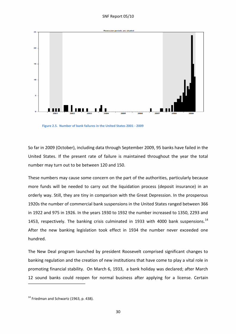
significantly, however, as shown in Figure 2.5.
SNF Report 05/10
30
Figure 2.5. Number of bank failures in the United States 2001 - 2009
So far in 2009 (October), including data through September 2009, 95 banks have failed in the
United States. If the present rate of failure is maintained throughout the year the total
number may turn out to be between 120 and 150.
These numbers may cause some concern on the part of the authorities, particularly because
more funds will be needed to carry out the liquidation process (deposit insurance) in an
orderly way. Still, they are tiny in comparison with the Great Depression. In the prosperous
1920s the number of commercial bank suspensions in the United States ranged between 366
in 1922 and 975 in 1926. In the years 1930 to 1932 the number increased to 1350, 2293 and
1453, respectively. The banking crisis culminated in 1933 with 4000 bank suspensions.14
After the new banking legislation took effect in 1934 the number never exceeded one
hundred.
The New Deal program launched by president Roosevelt comprised significant changes to
banking regulation and the creation of new institutions that have come to play a vital role in
promoting financial stability. On March 6, 1933, a bank holiday was declared; after March
12 sound banks could reopen for normal business after applying for a license. Certain
14 Friedman and Schwartz (1963, p. 438).
SNF Report 05/10
31
national banks with impaired assets were later allowed to open for business on a restricted
basis subject to approval from the authorities. Such banks could receive new deposits, which
were segregated from other liabilities of the bank; these were available for immediate
withdrawal without restrictions. These measures, in conjunction with a far more expansive
monetary policy stance, seem to have brought about financial stability again. Soon after this
the economy turned upward.
The Glass-Steagall Act set up the Federal Deposit Insurance Corporation (FDIC), which
provided insurance on deposits. After this scheme came into operation at the beginning of
1934, the problem of virulent bank runs disappeared. Another important piece of legislation
concerned cross ownership in the banking sector. The activities of the investment bank arms
were seen to be involved in highly risky operations, often of a speculative character, which
was not compatible with sound banking funded by ordinary bank deposits. The investment
banks were accordingly segregated from the commercial banks.
There is much agreement about the crucial role played by the banking crises during the
Great Depression. This is perhaps the most unique feature of this episode. If we were to
single out one factor that could explain why this cycle was so severe – which is probably a
too gross simplification to be taken seriously, though – it is certainly the bank failures.
The bank crises occupy a prominent place in Friedman and Schwartz’ (1963, pp. 299-419)
authoritative historical narrative of the Great Contraction. They describe three successive
waves of bank failures in 1930, 1931 and 1933, each more severe than the preceding one.
The Federal Reserve System did show some concern about the wave of bank failures
towards the end of 1930, in particular the failure of the Bank of the United States in
December 1930, the largest bank ever to have failed up to that time. But in general few
significant measures were taken by the Federal Reserve to stem the tide of bank failures
until the Emergency Banking Act of March 1933 was launched by the newly elected
president Roosevelt as part of the New Deal program. The reasons for this ineptitude on the
part of the monetary authorities are believed to be rooted in the fact that most failed banks
were small, and many were not members of the Federal Reserve System. Many cases of
bankruptcy were also regarded as a consequence of bad management and bad banking
practices, and, for moral reasons, therefore not to be assisted by central bank action.
SNF Report 05/10
32
In retrospect, there is no doubt that the lack of intervention on the part of the Federal
Reserve System to alleviate the banking problems prior to March 1933 was a major policy
failure. In the view of Friedman and Schwartz (1963, p. 358): ‘The major reason the System
was so belated in showing concern about bank failures and so inactive in responding to them
was undoubtedly limited understanding of the connection between bank failures, runs on
banks, contractions of deposits, and weakness of the bond markets.’
The credit crunch
Ben Bernanke is one of the leading academic experts on the causes and effects of the
financial crisis of the interwar period. In a famous paper Bernanke (1983) attaches a crucial
role to the behavior of the banks during the Great Contraction. He defines the concept of
the Cost of Credit Intermediation (CCI) as being the cost of channeling funds from ultimate
savers (and thus lenders) into the hands of good borrowers. The CCI will typically include
screening, monitoring, and accounting costs in addition to expected losses from the banks’
failing borrowers. Banks occupy a key role in the credit intermediation process; because of
asymmetric information problems households and many small businesses are excluded from
raising capital from the securities markets. Only banks possess the necessary resources to
screen and monitor the borrowers’ economic situation. As a consequence these borrowers
are dependent on bank credit for spending beyond their cash flow. The amounts of credit
extended to such borrowers are determined by the banks’ ability and willingness to lend as
well as the assessment of the borrowers’ future earnings and the value of the collateral that
can be provided.
In any major economic downturn the price of collateral will decline, earning prospects will
deteriorate and the number of bankruptcies will increase. Expected losses are thus likely to
increase. All these features of a major recession tend to increase the cost of credit
intermediation to the banks. The more severe and protracted the recession period is, the
more CCI will increase.
The banks’ response to this situation entails a potentially important repercussion on the
business cycle. To the extent that banks increase the rate of interest they charge borrowers
relative to their funding costs, less credit will be the result (the supply curve shifts upwards
SNF Report 05/10
33
and to the left in the market for bank credit). During a recession a normal response for banks
is to tighten their credit standards, so that loans may be refused to borrowers who were
previously granted loans. If conditions become sufficiently bad the banks may curtail their
lending significantly, in particular to applicants about which the bank has little or no prior
information. When many banks fail, as was the case in the years 1930-1933, a significant
number of potential borrowers may have been affected by these mechanisms.
Bernanke (1983, p. 257) believes that it was this type of credit crunch that was the
distinguishing feature of the Great Contraction: ‘As the real costs of intermediation
increased, some borrowers (especially households, farmers, and small firms) found credit to
be expensive and difficult to obtain. The effects of this credit squeeze on aggregate demand
helped convert the severe, but not unprecedented, downturn of 1929-30 into a protracted
depression.’
Whereas Friedman and Schwartz (1963) emphasized the money supply as the crucial link
between the bank failures and the downward spiraling economy, Bernanke (1983) focuses
more explicitly on the credit intermediation process. These approaches may be seen as
complementary rather than conflicting, although the latter transmission mechanism seems
to provide a deeper understanding of the banks’ special role in this case. Both contributions
add significantly to our understanding of the crucial role of money and credit as to their
effects on the real economy in any major financial crisis.
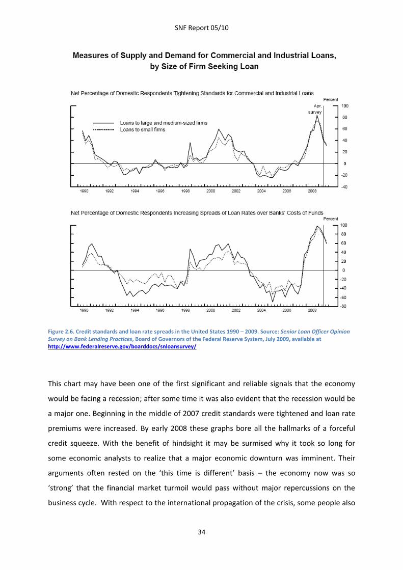
The credit crunch mechanism described above is also believed to be a major feature of the
transmission of contractionary impulses in the present financial crisis. In late 2007, and
certainly in early 2008, it became evident that banks responded to the financial market
turmoil by tightening credit standards and raising their lending rates relative to funding
costs. This is shown in Figure 2.6, which is an updated graph of the results of the bank credit
survey conducted by the Federal Reserve Board, that has been freely available on their
home page throughout the crisis (and earlier).
SNF Report 05/10
34
Figure 2.6. Credit standards and loan rate spreads in the United States 1990 – 2009. Source: Senior Loan Officer Opinion Survey on Bank Lending Practices, Board of Governors of the Federal Reserve System, July 2009, available at http://www.federalreserve.gov/boarddocs/snloansurvey/
This chart may have been one of the first significant and reliable signals that the economy
would be facing a recession; after some time it was also evident that the recession would be
a major one. Beginning in the middle of 2007 credit standards were tightened and loan rate
premiums were increased. By early 2008 these graphs bore all the hallmarks of a forceful
credit squeeze. With the benefit of hindsight it may be surmised why it took so long for
some economic analysts to realize that a major economic downturn was imminent. Their
arguments often rested on the ‘this time is different’ basis – the economy now was so
‘strong’ that the financial market turmoil would pass without major repercussions on the
business cycle. With respect to the international propagation of the crisis, some people also
SNF Report 05/10
35
referred on the decoupling hypothesis, arguing that the strong underlying growth rates of
Asian economies would prevent the crisis from affecting the rest of the world. This turned
out to be wrong, not least because the same tendencies of a credit crunch hit many
countries throughout the world.
With respect to policy directed towards troubled banks and the importance of deposit
insurance the crucial lessons from the Great Depression have been learnt and implemented
a long time ago. The swift and forceful actions taken by the Fed during the present crisis
demonstrate this point fully. Other lessons seem to have to be relearned over and over
again, however. One such issue is cross ownership in the banking world. The Gramm-Leach-
Bliley Act of 1999, which repealed the Glass-Steagall Act, removed the restrictions on the
affiliation of investment banks and commercial banks. Some observers have pointed to the
liberalization of these ties as a source of financial instability during the present financial
crisis.15
Monetary policy
Two key indicators of the stance of monetary policy are the discount rate (or more generally,
the rate of interest at which banks can borrow from the Fed) and the amount of base money
that the central bank supplies to the banking sector through open market operations and
various lending facilities. On the basis of such indicators monetary policy during the Great
Contraction is perhaps best described as rather inconsistent and mis-managed.
The traditional cyclical pattern of interest policy is an increase in discount rates prior to the
peak, often with a view to deflate asset prices, which tend to rise markedly in the late stages
of a boom period. The increase in the discount rate from 5 to 6 percent early in 1929 may
have been just such a move. The stock market crash of October 1929 is strong evidence that
this aim was thoroughly achieved. The side effect is of course that it probably triggered the
downturn of the economy as well – but this outcome is not exceptional. Discount rates were
15 The five largest investment banks, including Bear Stearns, submitted to voluntary supervision by the
Securities and Exchange Commission (SEC). However, they nevertheless managed to take huge risks while
under the oversight of the SEC. See Mizen (2008).
SNF Report 05/10
36
reduced in many steps during 1930, reaching a low of 1.5 per cent at the end of the year. But
as a response to the international financial market turmoil in the autumn of 1931, when
Britain and Scandinavian countries left gold, the discount rate was raised abruptly to 3.25
per cent and it hovered around 3 per cent during the rest of the contraction period. Because
the general price level had been falling for a long time, price expectations were surely
negative, which made expected real interest rates very high.
Regarding the other indicator of monetary policy, the monetary base, the policy was roughly
neutral until the end of 1931. Some attempts were periodically made to provide the banking
sector with more liquidity, but this was partially reversed during other periods. It was only in
1932, when the crisis had lasted almost three years, that a more systematic injection of
liquidity was undertaken.
According to Friedman and Schwartz (1963) there are two main reasons why monetary
policy stands out as so half-hearted and inept during this period. The first reason is the lack
of understanding in the Federal Reserve System of the need for a forceful monetary
expansion during the exceptional circumstances. There were strongly conflicting views on
this issue within the Federal Reserve System at the time, which led to an inconsistent policy.
The second reason is the constraints on monetary policy that the gold standard entailed.
Our understanding of the proper conduct of monetary policy has gained a lot from the Great
Contraction episode. The mistakes made then have surely influenced the actions taken in the
present crisis. This time all available guns were fired in a swift and decisive action: interest
rates were pushed to the extreme lower bound and huge amounts of liquidity were injected
into the money markets.
The recovery phase: what are the lessons from the Great Contraction?
Here we focus briefly on some issues related to the conduct of monetary policy in the
aftermath of the 1929-1933 recession, which have some striking parallels in the current
cycle. The lessons learnt from the handling of these issues in the 1930s clearly warrant
further attention in the coming years. At present there are, of course, many other aspects of
the unwinding of the massive countercyclical policy measures that were taken in 2008-2009,
SNF Report 05/10
37
in particular the huge accumulation of government debt following from the financial market
rescue operations and fiscal policy stimulus, but a discussion of this is beyond the scope of
this chapter.
What led out of the recession?
It seems to be well established by now that the recovery in the United States after the
trough of the cycle was reached in 1933 was mainly due to monetary expansion. According
to Christina Romer (1992, 2009) fiscal policy was of some importance, but not the key engine
of growth in the following years. Although Roosevelt’s spending programs implied large
federal budget deficits, state and local governments were running surpluses. The net effect
was a deficit of one and a half percent of gross domestic product in 1934 (compared to a
fiscal stimulus of about 3 percent now). The fiscal expansion was not unimportant, as it
signaled a break with the balanced budget of previous years, but it was not sustained,
however. Therefore monetary policy stands out as the most persistent and forceful
expansive factor behind the strong revival that lasted until 1937.
The expansionary monetary policy does not stem primarily from the fact that interest rates
were kept low – as they were already at a low level in 1933 they could not get much lower –
but rather from an early example of quantitative easing. After the suspension of gold
payments in March 1933 a significant devaluation of the dollar in terms of gold took place in
the markets. A new official price of USD 35 per ounce gold was set in February 1934. As
capital started to flow from Europe to the United States the Treasury decided not to sterilize
the gold inflow. By issuing gold certificates, which were interchangeable with Federal
Reserve notes, the Treasury was able to increase the money supply at a rate of 17 per cent
per year between 1933 and 1936, without involving the central bank.
SNF Report 05/10
38
Monetary policy in the aftermath of the recession – coping with changes in risk attitude, liquidity preference and lending behavior of the banks
The huge monetary expansion in the mid-1930s resulted in mounting bank reserves.
Whereas depositor runs on banks and gold outflows caused bank reserves to contract
sharply during the 1929-33 cycle, this situation was radically reversed when the economic
policy change introduced by Roosevelt came into effect. Federal deposit insurance increased
the depositors’ confidence in the solidity of banks and gold inflows were allowed to affect
the money supply, as explained above.
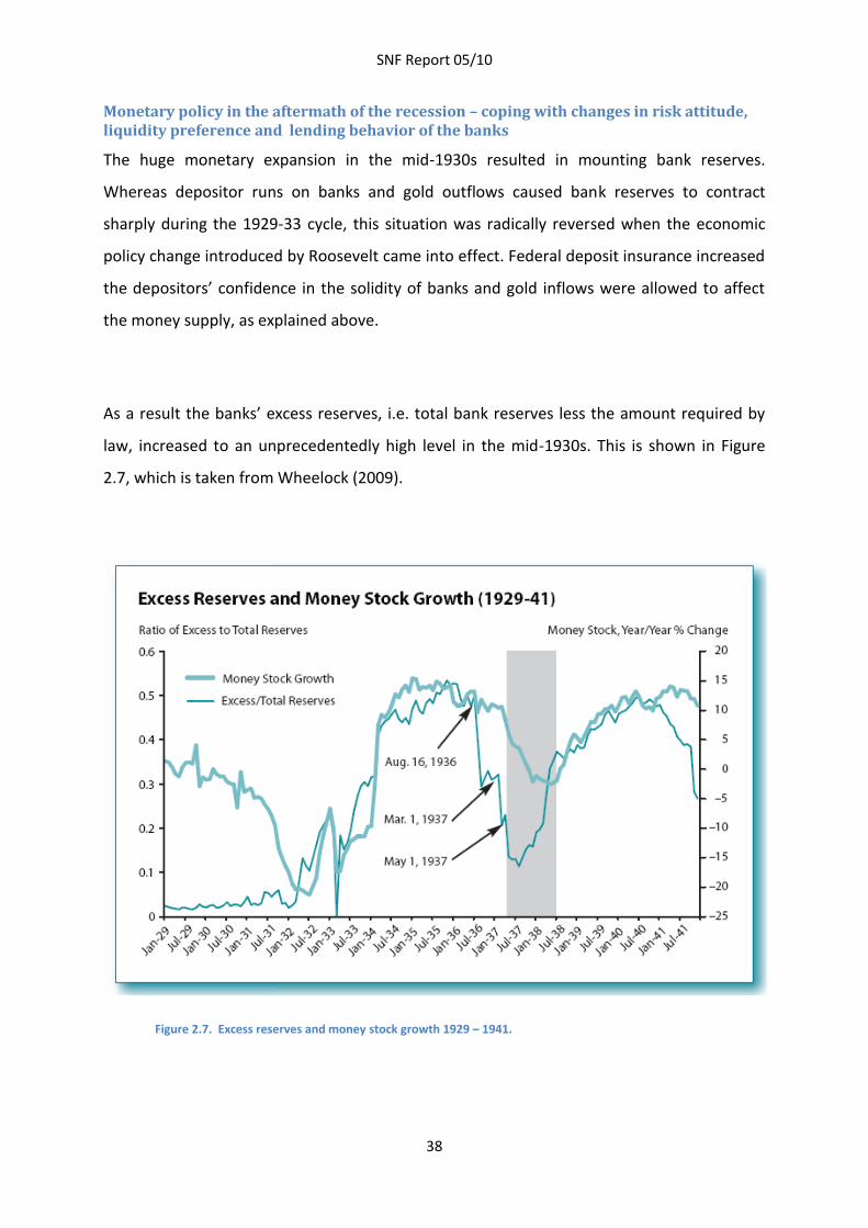
As a result the banks’ excess reserves, i.e. total bank reserves less the amount required by
law, increased to an unprecedentedly high level in the mid-1930s. This is shown in Figure
2.7, which is taken from Wheelock (2009).
Figure 2.7. Excess reserves and money stock growth 1929 – 1941.
SNF Report 05/10
39
The thin line is excess reserves as a fraction of total reserves. As can be seen from this graph
the turnaround in the banks’ liquidity position in 1933 was accompanied by monetary
expansion. When banks got their funding under control, they could start lending again.
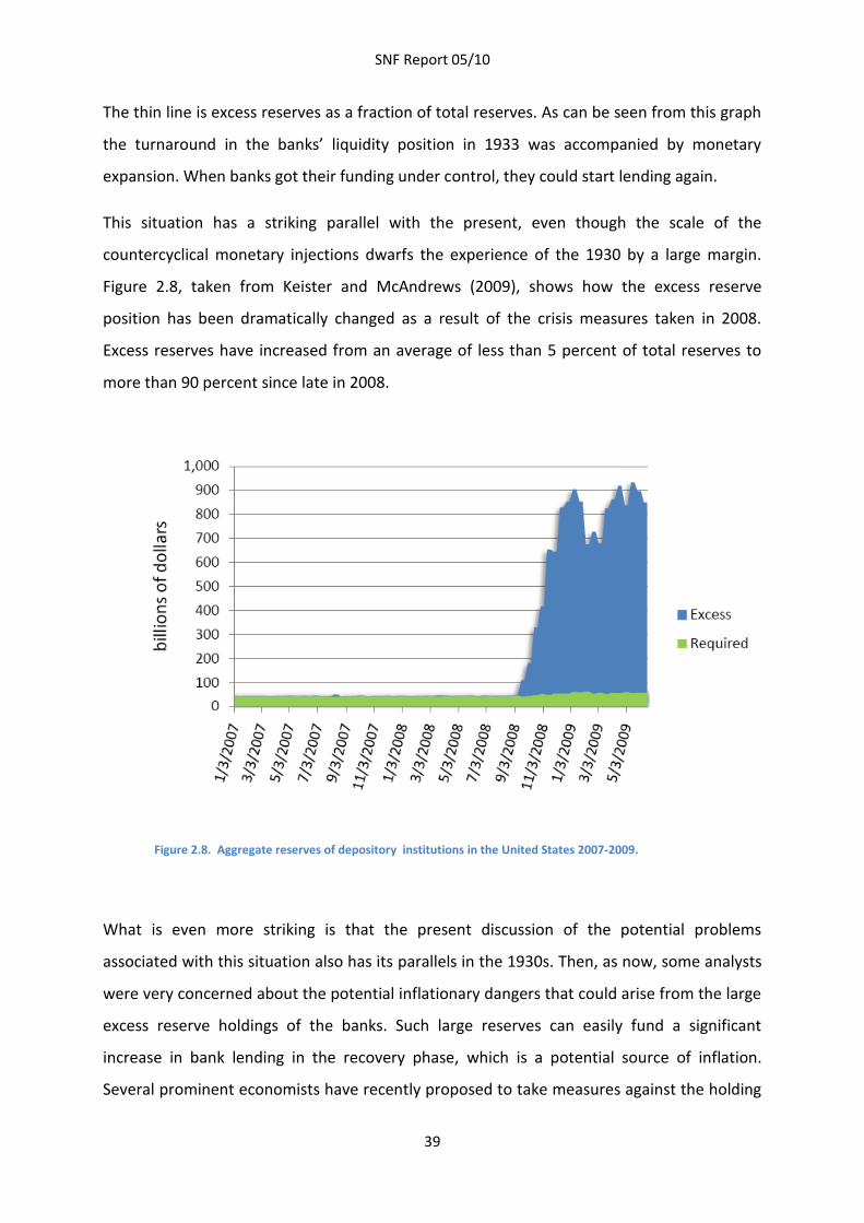
This situation has a striking parallel with the present, even though the scale of the
countercyclical monetary injections dwarfs the experience of the 1930 by a large margin.
Figure 2.8, taken from Keister and McAndrews (2009), shows how the excess reserve
position has been dramatically changed as a result of the crisis measures taken in 2008.
Excess reserves have increased from an average of less than 5 percent of total reserves to
more than 90 percent since late in 2008.
Figure 2.8. Aggregate reserves of depository institutions in the United States 2007-2009.
What is even more striking is that the present discussion of the potential problems
associated with this situation also has its parallels in the 1930s. Then, as now, some analysts
were very concerned about the potential inflationary dangers that could arise from the large
excess reserve holdings of the banks. Such large reserves can easily fund a significant
increase in bank lending in the recovery phase, which is a potential source of inflation.
Several prominent economists have recently proposed to take measures against the holding
SNF Report 05/10
40
of such large excess reserves by imposing taxes on reserve holdings or enforcing more direct
regulatory measures.16
Responding to just such concerns the Federal Reserve decided in 1936 to reduce excess
reserves by increasing reserve requirements in three steps between August 1936 and May
1937. This made it more costly for the banks to grant new loans, encouraging banks to
reduce lending. As is evident from Figure 2.8, this resulted in a marked contraction of the
growth rate of the money stock. If we refer back to Figure 2.1, it is seen that the economy
entered an unusually steep economic downturn just as this contractionary monetary policy
was taking effect in the middle of 1937. It is thoroughly documented in Friedman and
Schwartz (1963) and Romer (1992) that a main cause of this cycle was the severe monetary
contraction, although there was also a fairly strong fiscal contraction at the same time.
The lesson from this episode is clear. During, and perhaps for a considerable time after a
crisis, banks change their behavior as a precautionary measure. They definitely want to
increase their reserve holdings, both because they have experienced that liquidity may be
difficult to obtain if the financial turmoil returns and because they are reluctant to lend to
other banks due to increased perceived counterparty risk. They also tighten credit standards
and are more reluctant to engage in lending to customers because the assessment of
borrowers’ earning prospects has deteriorated. The behavior of banks is often heavily
criticized on this account, in particular from representatives of the business community who
have not been able to obtain the loans they had been used to in the boom period. The
response of the banks is probably to a large extent rational, reflecting the increased cost of
credit intermediation. In any case, it is a response on the part of the banking sector that
students of interwar banking history are familiar with.
Financial crises and the economy of Norway in the interwar period
The brief survey of the lessons from the effects of the financial crisis on the economy of the
United States in the 1930s has shown that important policy lessons have already been learnt
16 See Keister and McAndrews (2009) for references.
SNF Report 05/10
41
from this episode. More research efforts on these issues are obviously needed, and are likely
to be of great interest to policy makers. Although further lessons from the U.S. economy
may be welcome, it can also be argued that it would be fruitful to shift the focus to other
countries as well.
We present a brief, tentative outline of some of the issues that would be particularly
relevant to the Norwegian case.
The banking crises and their effects on business cycles and exchange rates
In Norway the most severe banking crisis was not associated with the Great Contraction
period but occurred in the first part of the 1920s. Recently, there has been an important
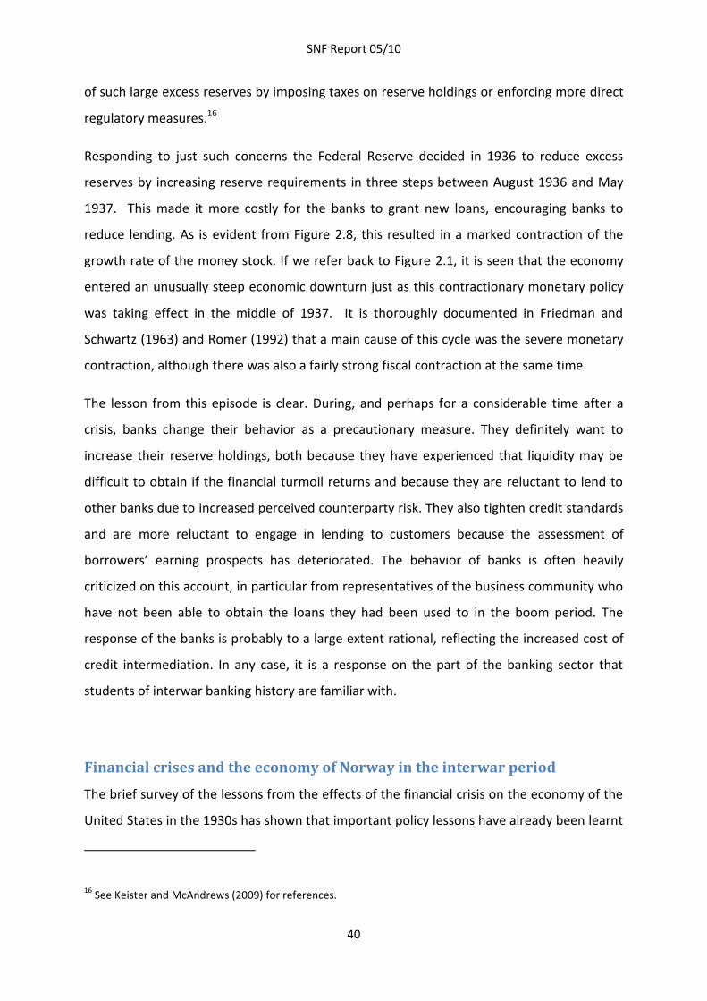
revision of the timing of the losses incurred by the commercial banks in the 1920s. Knutsen
(2007) has shown that the old estimates made by Statistics Norway give a misleading
picture, see Figure 2.9. His new estimates shift the losses considerably forward in time,
peaking in 1922 rather than in 1925, as indicated by the Statistics Norway data. One
implication of this finding is that the banking crisis was not primarily due to the strong
appreciation of the krone starting in the summer of 1924; rather, the attention is cast
backwards towards the reckless fiscal and monetary policy during the First World War and
its immediate aftermath.
Norway (and Denmark) was rather unique in experiencing a severe economic downturn in
1925-1926. This was a cycle which was hardly noticeable in other countries, such as for
example Sweden. The econometric results in Klovland (1998) are consistent with the
conventional view that this cycle was largely driven by exchange rate appreciation and
domestic monetary policy. The role played by the banking crisis is less established, however,
but well worth looking into more closely.
SNF Report 05/10
42
Figure 2.9. Norwegian commercial banks: losses in percent of total assets (SSB = Statistics Norway, Knutsen (2007))
Bank behavior during and after the crisis
We do not have much systematic knowledge about how banks behaved during and after the
crisis. How did they respond to the demands of their loan customers? How severe was the
credit crunch? What happened after the crisis with respect to reserve behavior and the
provision of credit?
On the background of the experience in the 1930s in the United States, and in both Norway
and other countries during the present cycle, it would not be surprising if there was a
tendency for banks to hoard liquid assets and tighten their credit standards.
The choice of monetary regime and the international propagation of business cycle
impulses
In relative terms Norway escaped lightly from the international business cycle depression
starting in 1929. The departure from gold in September 1931 may have been a key factor
here. This is consistent with the results in Eichengreen and Sachs (1985), who showed that
the single most important factor in explaining the performance of the European economies
in the 1930s was the point in time when the country in question abandoned the gold
standard. A closer look at this episode from a Norwegian perspective may shed some light
on the properties of fixed exchange rate regimes during a financial crisis.
SNF Report 05/10
43
Financial crises and economic growth in the interwar years
No other period has been so thoroughly marked by economic crises as the interwar years:
bank crises, unprecedented exchange rate shocks (the krone doubling its international value
over a period of two to three years) as well as international financial crises and deflationary
impulses. Yet the economic growth record of Norway during these years is remarkably good.
Figure 2.10 shows 5-year end-of-period growth rates for gross domestic product in Norway
for a period of nearly 140 years. It will be seen that, once the difficult years at the end of
World War I and the international business cycle downturn thereafter had passed, the
growth of the Norwegian economy was fairly strong during the rest of the interwar period.
Figure 2.10. 5-year end-of-period growth rates in GDP 1871 - 2008
It is indeed somewhat puzzling to note that the growth record of the interwar years was
almost comparable to the first decades of the post-WWII era, and significantly better than in
the decades prior to about 1910 as well as in the 1970s and 1980s. Some differences may be
due to demographic trends, which are not accounted for here, but the resilience of the
Norwegian economy is still remarkable during the decades plagued by financial market
turmoil. A tentative, but probably too imprecise hypothesis, may be that financial crises
cause business cycle fluctuations but that they are not particularly important for long-run
economic growth.
SNF Report 05/10
44
Chapter 3: Determinants of Financial Crises
This chapter reviews the literature on the following types of financial crises: (1) banking, (2)
currency, (3) combinations of these two, so-called twin crises, and (4) debt crises. The
chapter discusses empirical determinants of financial crises for a number of emerging
market and developed economies. We discuss typical paths of recovery and growth after
financial crises and contrast this pattern with experience in Nordic countries in the 1990s.
The chapter concludes with lessons for economic policy.
Typical financial crises
An illustrative model of financial crises was developed by Hyman Minsky (1982). Following
Minsky, the typical timing of events leading to financial crises can be decomposed into
different stages which are illustrated in Figure 3.1. Kindleberger and Aliber (2005) describe
timing of events of “typical” financial crises that have repeatedly occurred in the past 400
years.17
At the onset of many crises one can observe an initial shock, such as financial liberalization
or exogenous increases in the supply or demand of credit. In the context of the recent
financial crises that started in 2007, the increase in global savings or “savings glut” (cf.
Bernanke, 2005), low interest rates and financial deregulation in the 1990s have been
suggested in the literature. Following the initial shock, one can observe a strong expansion of
credit, which can be explained by increased demand by firms due to rising expected
profitability and also the boost in supply fueled by reduced risk awareness. The increased
availability of credit leads to a boom in the economy reinforcing the initial shock.
17 See Kindleberger and Aliber (2005, pp. 256-265) for a stylized outline of financial crises from 1618 to 1998.
For an even longer perspective see Reinhart and Rogoff (2009a), documenting 800 years of financial folly.
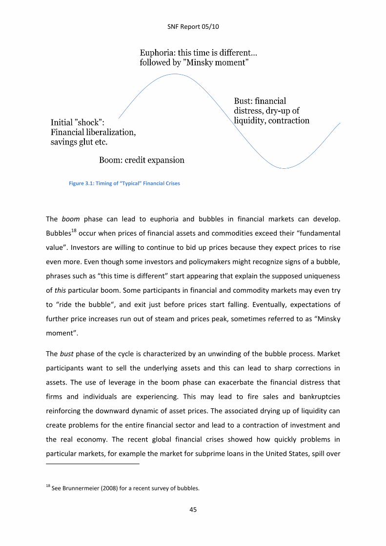
SNF Report 05/10
45
Figure 3.1: Timing of “Typical” Financial Crises
The boom phase can lead to euphoria and bubbles in financial markets can develop.
Bubbles18 occur when prices of financial assets and commodities exceed their “fundamental
value”. Investors are willing to continue to bid up prices because they expect prices to rise
even more. Even though some investors and policymakers might recognize signs of a bubble,
phrases such as “this time is different” start appearing that explain the supposed uniqueness
of this particular boom. Some participants in financial and commodity markets may even try
to “ride the bubble“, and exit just before prices start falling. Eventually, expectations of
further price increases run out of steam and prices peak, sometimes referred to as “Minsky
moment”.
The bust phase of the cycle is characterized by an unwinding of the bubble process. Market
participants want to sell the underlying assets and this can lead to sharp corrections in
assets. The use of leverage in the boom phase can exacerbate the financial distress that
firms and individuals are experiencing. This may lead to fire sales and bankruptcies
reinforcing the downward dynamic of asset prices. The associated drying up of liquidity can
create problems for the entire financial sector and lead to a contraction of investment and
the real economy. The recent global financial crises showed how quickly problems in
particular markets, for example the market for subprime loans in the United States, spill over
18 See Brunnermeier (2008) for a recent survey of bubbles.
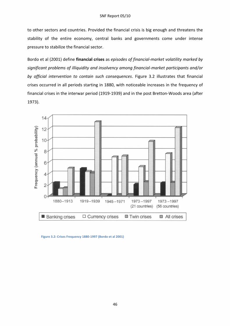
SNF Report 05/10
46
to other sectors and countries. Provided the financial crisis is big enough and threatens the
stability of the entire economy, central banks and governments come under intense
pressure to stabilize the financial sector.
Bordo et al (2001) define financial crises as episodes of financial-market volatility marked by
significant problems of illiquidity and insolvency among financial-market participants and/or
by official intervention to contain such consequences. Figure 3.2 illustrates that financial
crises occurred in all periods starting in 1880, with noticeable increases in the frequency of
financial crises in the interwar period (1919-1939) and in the post Bretton-Woods area (after
1973).
Figure 3.2: Crises Frequency 1880-1997 (Bordo et al 2001)
SNF Report 05/10
47
Banking crises
A banking crisis can be defined as an episode of financial distress resulting in erosion of most
or all of aggregate banking system capital (cf. Bordo et al, 2001). Calomiris (2008) argues
that banking crises greatly differ in their severity and source of the crisis, originating either
within or outside the banking system. Calomiris also observes that all major US banking
panics occurred at business cycle peaks and were preceded by spikes in liabilities of failed
businesses. Figure 3.3 shows incidence of banking crises.
Reinhart and Rogoff (2008a) make the following observations about the incidence of banking
crises: historically, global banking crises were associated with sovereign defaults of external
debt; waves of global financial distress occurred in earlier periods (for example, the Panic of
1907 or the outbreak of the First World War); the relative calm during the late 1940s to the
early 1970s can be partly explained by repression of domestic markets and capital controls;
since the 1970s, financial and capital account liberalization has taken place, but we also
observe the recurrence of banking crises; both advanced and emerging economies are
affected, and one can often observe serial incidence of banking crises.
Reinhart and Rogoff (2009) argue that the same relationship that occurred between the
resurgence of financial crises following the liberalization in the 1970s can also be found
historically. Figure 3.4 shows the relationship between an index of capital mobility,
calculated by Obstfeld and Taylor (2004), and a three-year moving average of the share of
countries experiencing a banking crises. Observe the rise in capital mobility in the late 19th
century up until World War I, and the U-shaped pattern in the 20th century, and a similar
timing of incidences of banking crises. Kaminsky and Reinhart (1999) document that 18 out
of 26 banking crises after the 1970s follow financial liberalization in the preceding five years.
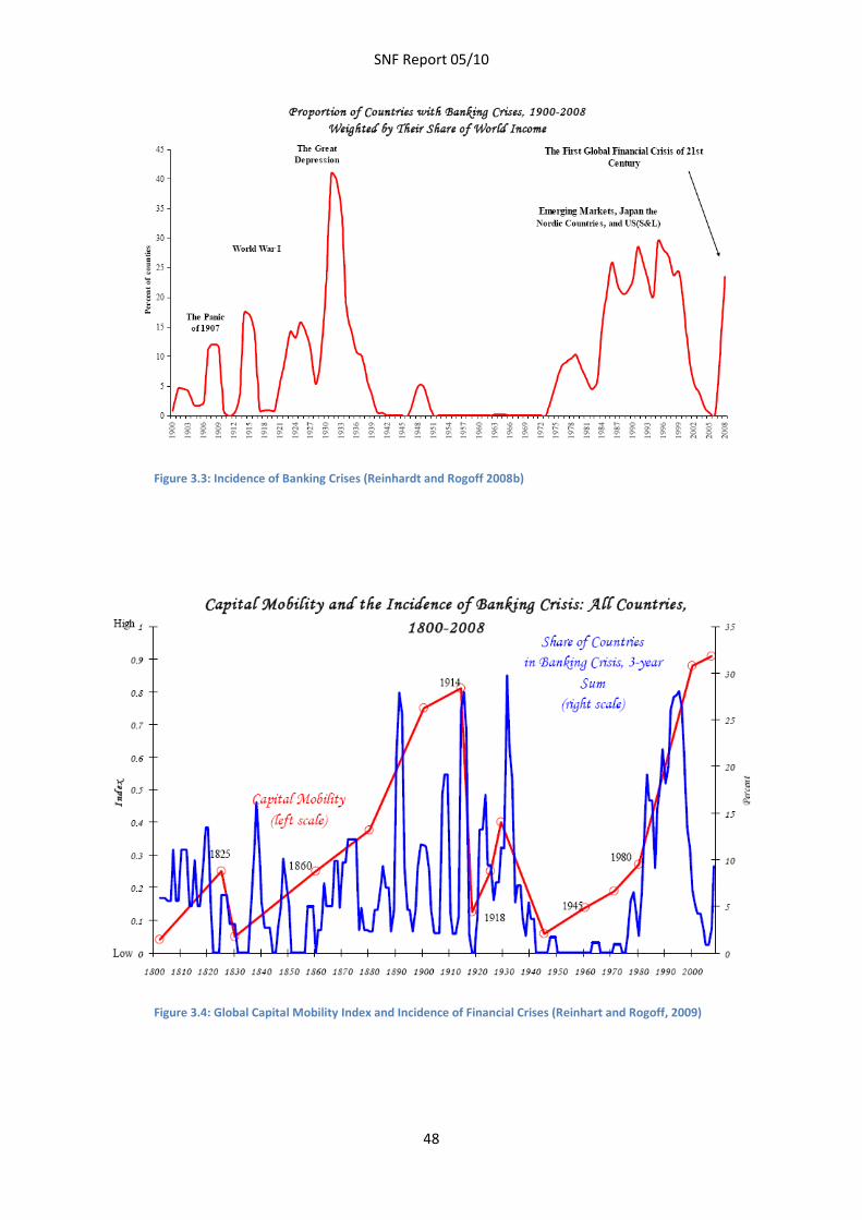
SNF Report 05/10
48
Figure 3.3: Incidence of Banking Crises (Reinhardt and Rogoff 2008b)
Figure 3.4: Global Capital Mobility Index and Incidence of Financial Crises (Reinhart and Rogoff, 2009)
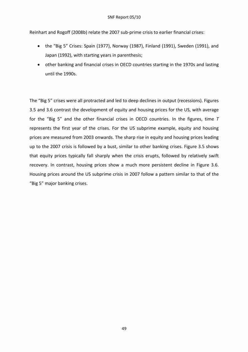
SNF Report 05/10
49
Reinhart and Rogoff (2008b) relate the 2007 sub-prime crisis to earlier financial crises:
the “Big 5” Crises: Spain (1977), Norway (1987), Finland (1991), Sweden (1991), and
Japan (1992), with starting years in parenthesis;
other banking and financial crises in OECD countries starting in the 1970s and lasting
until the 1990s.
The “Big 5” crises were all protracted and led to deep declines in output (recessions). Figures
3.5 and 3.6 contrast the development of equity and housing prices for the US, with average
for the “Big 5” and the other financial crises in OECD countries. In the figures, time T
represents the first year of the crises. For the US subprime example, equity and housing
prices are measured from 2003 onwards. The sharp rise in equity and housing prices leading
up to the 2007 crisis is followed by a bust, similar to other banking crises. Figure 3.5 shows
that equity prices typically fall sharply when the crisis erupts, followed by relatively swift
recovery. In contrast, housing prices show a much more persistent decline in Figure 3.6.
Housing prices around the US subprime crisis in 2007 follow a pattern similar to that of the
“Big 5” major banking crises.
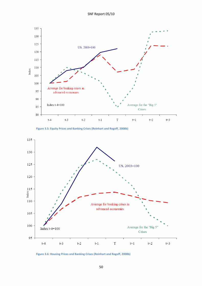
SNF Report 05/10
50
Figure 3.5: Equity Prices and Banking Crises (Reinhart and Rogoff, 2008b)
Figure 3.6: Housing Prices and Banking Crises (Reinhart and Rogoff, 2008b)
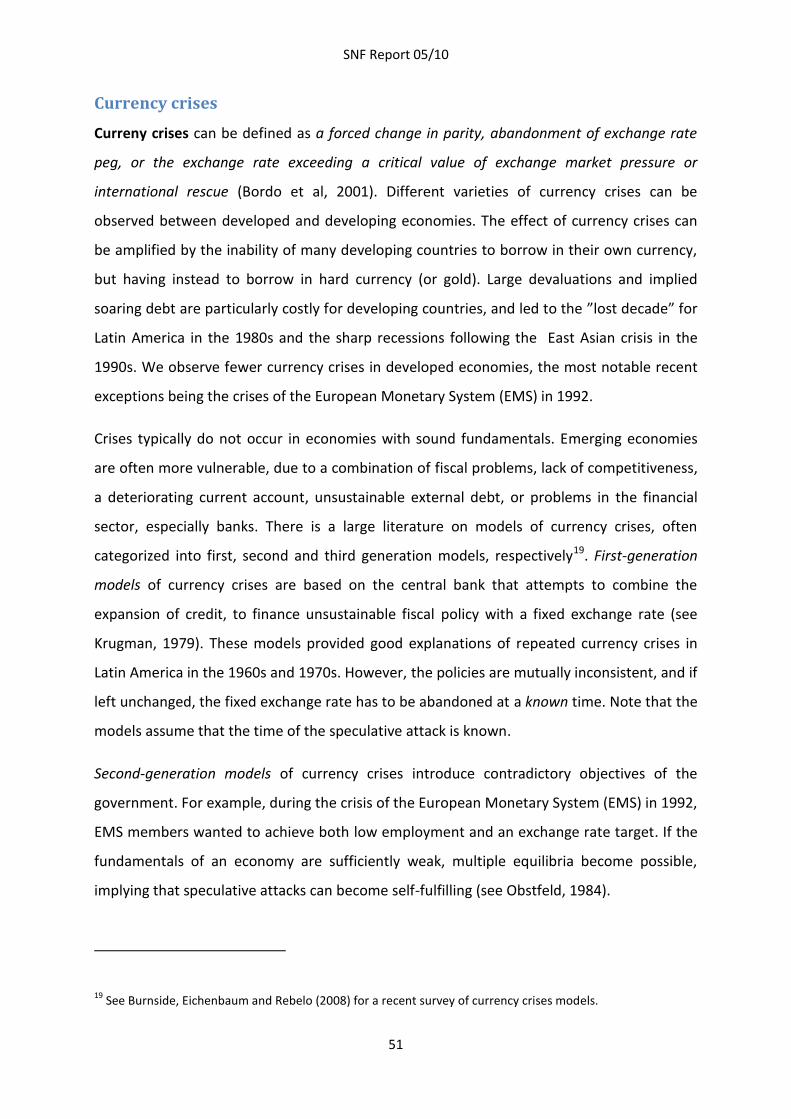
SNF Report 05/10
51
Currency crises
Curreny crises can be defined as a forced change in parity, abandonment of exchange rate
peg, or the exchange rate exceeding a critical value of exchange market pressure or
international rescue (Bordo et al, 2001). Different varieties of currency crises can be
observed between developed and developing economies. The effect of currency crises can
be amplified by the inability of many developing countries to borrow in their own currency,
but having instead to borrow in hard currency (or gold). Large devaluations and implied
soaring debt are particularly costly for developing countries, and led to the ”lost decade” for
Latin America in the 1980s and the sharp recessions following the East Asian crisis in the
1990s. We observe fewer currency crises in developed economies, the most notable recent
exceptions being the crises of the European Monetary System (EMS) in 1992.
Crises typically do not occur in economies with sound fundamentals. Emerging economies
are often more vulnerable, due to a combination of fiscal problems, lack of competitiveness,
a deteriorating current account, unsustainable external debt, or problems in the financial
sector, especially banks. There is a large literature on models of currency crises, often
categorized into first, second and third generation models, respectively19. First-generation
models of currency crises are based on the central bank that attempts to combine the
expansion of credit, to finance unsustainable fiscal policy with a fixed exchange rate (see
Krugman, 1979). These models provided good explanations of repeated currency crises in
Latin America in the 1960s and 1970s. However, the policies are mutually inconsistent, and if
left unchanged, the fixed exchange rate has to be abandoned at a known time. Note that the
models assume that the time of the speculative attack is known.
Second-generation models of currency crises introduce contradictory objectives of the
government. For example, during the crisis of the European Monetary System (EMS) in 1992,
EMS members wanted to achieve both low employment and an exchange rate target. If the
fundamentals of an economy are sufficiently weak, multiple equilibria become possible,
implying that speculative attacks can become self-fulfilling (see Obstfeld, 1984).
19 See Burnside, Eichenbaum and Rebelo (2008) for a recent survey of currency crises models.
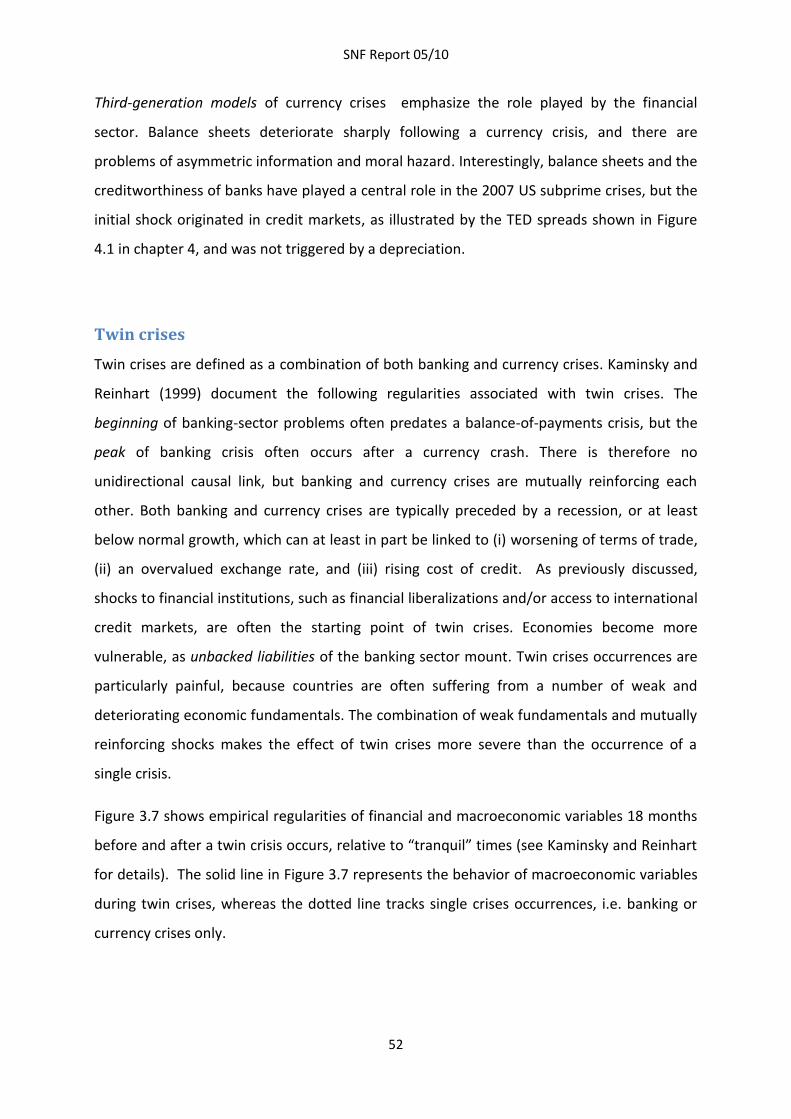
SNF Report 05/10
52
Third-generation models of currency crises emphasize the role played by the financial
sector. Balance sheets deteriorate sharply following a currency crisis, and there are
problems of asymmetric information and moral hazard. Interestingly, balance sheets and the
creditworthiness of banks have played a central role in the 2007 US subprime crises, but the
initial shock originated in credit markets, as illustrated by the TED spreads shown in Figure
4.1 in chapter 4, and was not triggered by a depreciation.
Twin crises
Twin crises are defined as a combination of both banking and currency crises. Kaminsky and
Reinhart (1999) document the following regularities associated with twin crises. The
beginning of banking-sector problems often predates a balance-of-payments crisis, but the
peak of banking crisis often occurs after a currency crash. There is therefore no
unidirectional causal link, but banking and currency crises are mutually reinforcing each
other. Both banking and currency crises are typically preceded by a recession, or at least
below normal growth, which can at least in part be linked to (i) worsening of terms of trade,
(ii) an overvalued exchange rate, and (iii) rising cost of credit. As previously discussed,
shocks to financial institutions, such as financial liberalizations and/or access to international
credit markets, are often the starting point of twin crises. Economies become more
vulnerable, as unbacked liabilities of the banking sector mount. Twin crises occurrences are
particularly painful, because countries are often suffering from a number of weak and
deteriorating economic fundamentals. The combination of weak fundamentals and mutually
reinforcing shocks makes the effect of twin crises more severe than the occurrence of a
single crisis.
Figure 3.7 shows empirical regularities of financial and macroeconomic variables 18 months
before and after a twin crisis occurs, relative to “tranquil” times (see Kaminsky and Reinhart
for details). The solid line in Figure 3.7 represents the behavior of macroeconomic variables
during twin crises, whereas the dotted line tracks single crises occurrences, i.e. banking or
currency crises only.
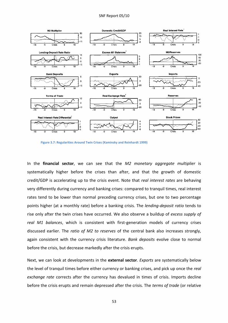
SNF Report 05/10
53
Figure 3.7: Regularities Around Twin Crises (Kaminsky and Reinhardt 1999)
In the financial sector, we can see that the M2 monetary aggregate multiplier is
systematically higher before the crises than after, and that the growth of domestic
credit/GDP is accelerating up to the crisis event. Note that real interest rates are behaving
very differently during currency and banking crises: compared to tranquil times, real interest
rates tend to be lower than normal preceding currency crises, but one to two percentage
points higher (at a monthly rate) before a banking crisis. The lending-deposit ratio tends to
rise only after the twin crises have occurred. We also observe a buildup of excess supply of
real M1 balances, which is consistent with first-generation models of currency crises
discussed earlier. The ratio of M2 to reserves of the central bank also increases strongly,
again consistent with the currency crisis literature. Bank deposits evolve close to normal
before the crisis, but decrease markedly after the crisis erupts.
Next, we can look at developments in the external sector. Exports are systematically below
the level of tranquil times before either currency or banking crises, and pick up once the real
exchange rate corrects after the currency has devalued in times of crisis. Imports decline
before the crisis erupts and remain depressed after the crisis. The terms of trade (or relative
SNF Report 05/10
54
price of exports over imports) deteriorate before the crisis, eroding purchasing power and
contributing relative price effects to the performance of net exports. Consistent with the
currency crises literature, foreign-exchange reserves of the central bank fall substantially in
the run-up to the crisis, and only recover once the currency devalues. Real interest rate
differentials do not change systematically before the crisis erupts, however they tend to be
systematically above normal before banking crises.
Finally, in the real sector, output growth and the development of stock prices start to slow
already before the crisis erupts, and show persistent weakness, particularly after twin crises
events.
Debt crises
External debt crises include outright default, but also repudiation or restructuring of debt
into less favorable terms for the lender (see Reinhart and Rogoff, 2009). In practice the
distinction between these definitions can be less sharp. For example, in the 2007 US sub-
prime crisis illiquidity and risk adjustment played an important role.
Bordo and Meissner (2006) and Reinhart and Rogoff (2009a) document that the following
factors are related to the occurrence of debt crises: currency mismatch, measured by the
ratio of hard currency debt to total debt; terms of trade fluctuations, and in particular spikes
in commodity prices; high levels of debt (relative to revenue or GDP); interest spreads, which
could be measures of reputation; a surge in global capital flows, so-called “bonanzas”,
followed by sudden stops or reversals of capital flows; finally, more generally, weak
economic fundamentals.
Reinhart and Rogoff (2009a) emphasize that domestic debt constitutes an important part of
government debt, including many emerging markets. They note that buildup of domestic
debt often occurs after external defaults, when countries find it difficult to borrow abroad.
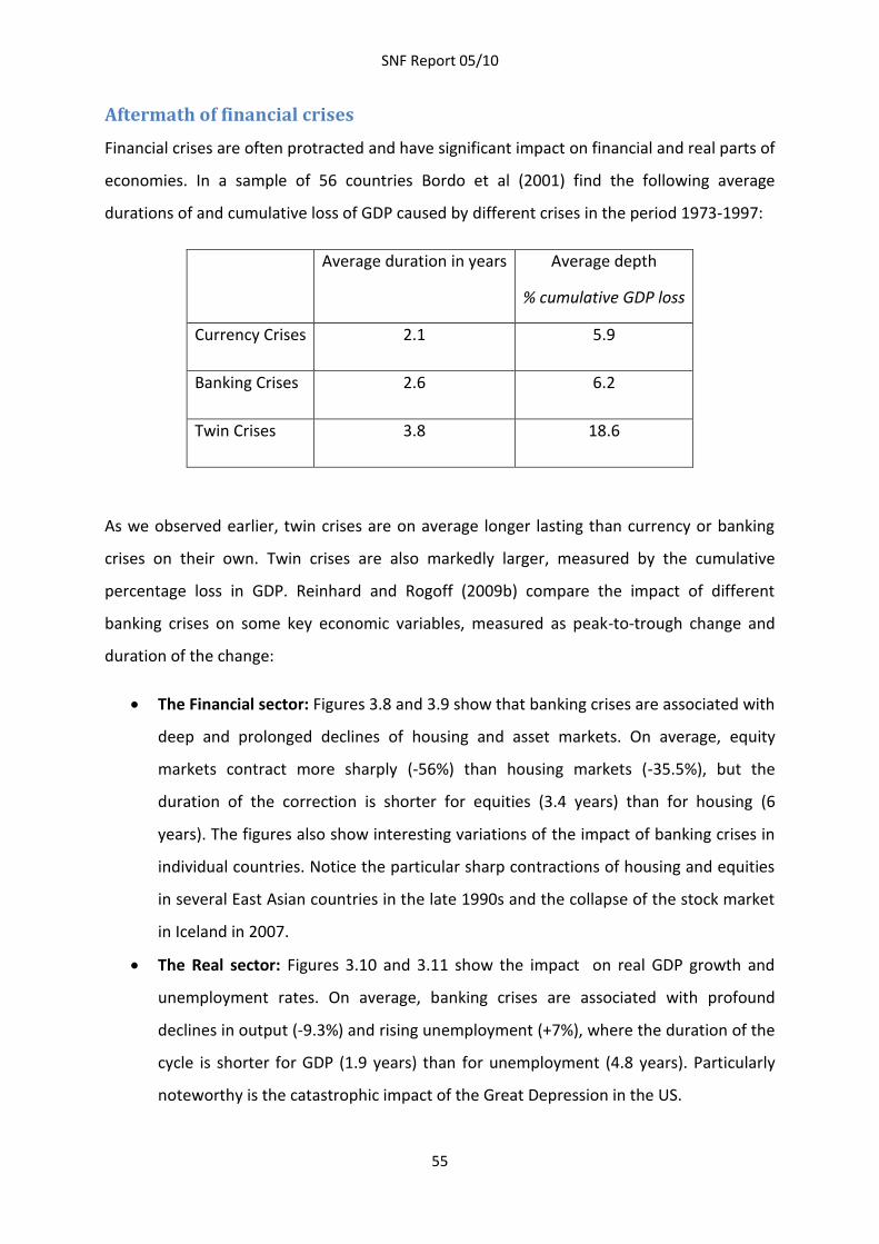
SNF Report 05/10
55
Aftermath of financial crises
Financial crises are often protracted and have significant impact on financial and real parts of
economies. In a sample of 56 countries Bordo et al (2001) find the following average
durations of and cumulative loss of GDP caused by different crises in the period 1973-1997:
Average duration in years Average depth
% cumulative GDP loss
Currency Crises 2.1 5.9
Banking Crises 2.6 6.2
Twin Crises 3.8 18.6
As we observed earlier, twin crises are on average longer lasting than currency or banking
crises on their own. Twin crises are also markedly larger, measured by the cumulative
percentage loss in GDP. Reinhard and Rogoff (2009b) compare the impact of different
banking crises on some key economic variables, measured as peak-to-trough change and
duration of the change:
The Financial sector: Figures 3.8 and 3.9 show that banking crises are associated with
deep and prolonged declines of housing and asset markets. On average, equity
markets contract more sharply (-56%) than housing markets (-35.5%), but the
duration of the correction is shorter for equities (3.4 years) than for housing (6
years). The figures also show interesting variations of the impact of banking crises in
individual countries. Notice the particular sharp contractions of housing and equities
in several East Asian countries in the late 1990s and the collapse of the stock market
in Iceland in 2007.
The Real sector: Figures 3.10 and 3.11 show the impact on real GDP growth and
unemployment rates. On average, banking crises are associated with profound
declines in output (-9.3%) and rising unemployment (+7%), where the duration of the
cycle is shorter for GDP (1.9 years) than for unemployment (4.8 years). Particularly
noteworthy is the catastrophic impact of the Great Depression in the US.
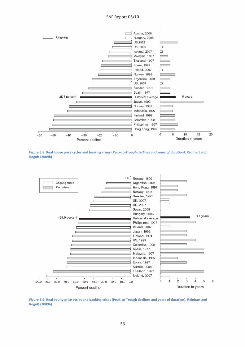
SNF Report 05/10
56
Figure 3.8: Real house price cycles and banking crises (Peak-to-Trough declines and years of duration), Reinhart and Rogoff (2009b)
Figure 3.9: Real equity price cycles and banking crises (Peak-to-Trough declines and years of duration), Reinhart and Rogoff (2009b)
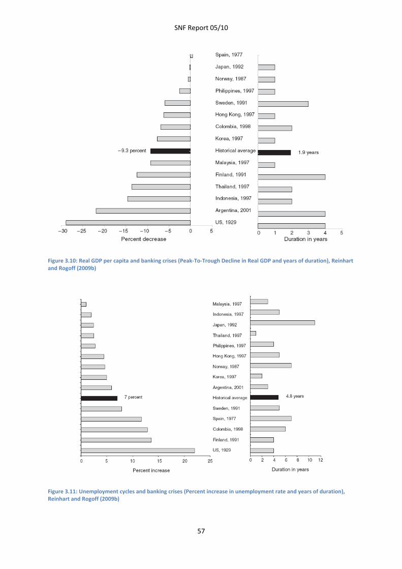
SNF Report 05/10
57
Figure 3.10: Real GDP per capita and banking crises (Peak-To-Trough Decline in Real GDP and years of duration), Reinhart and Rogoff (2009b)
Figure 3.11: Unemployment cycles and banking crises (Percent increase in unemployment rate and years of duration), Reinhart and Rogoff (2009b)
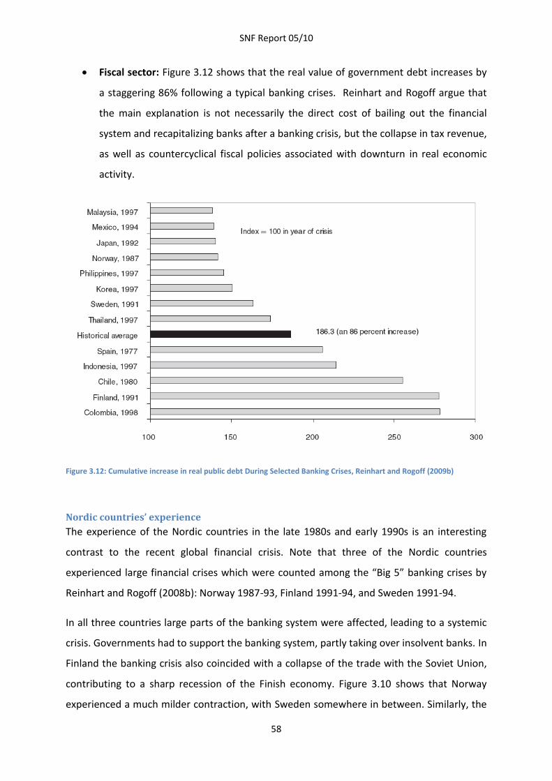
SNF Report 05/10
58
Fiscal sector: Figure 3.12 shows that the real value of government debt increases by
a staggering 86% following a typical banking crises. Reinhart and Rogoff argue that
the main explanation is not necessarily the direct cost of bailing out the financial
system and recapitalizing banks after a banking crisis, but the collapse in tax revenue,
as well as countercyclical fiscal policies associated with downturn in real economic
activity.
Figure 3.12: Cumulative increase in real public debt During Selected Banking Crises, Reinhart and Rogoff (2009b)
Nordic countries’ experience
The experience of the Nordic countries in the late 1980s and early 1990s is an interesting
contrast to the recent global financial crisis. Note that three of the Nordic countries
experienced large financial crises which were counted among the “Big 5” banking crises by
Reinhart and Rogoff (2008b): Norway 1987-93, Finland 1991-94, and Sweden 1991-94.
In all three countries large parts of the banking system were affected, leading to a systemic
crisis. Governments had to support the banking system, partly taking over insolvent banks. In
Finland the banking crisis also coincided with a collapse of the trade with the Soviet Union,
contributing to a sharp recession of the Finish economy. Figure 3.10 shows that Norway
experienced a much milder contraction, with Sweden somewhere in between. Similarly, the
SNF Report 05/10
59
cumulative increase in unemployment was largest for Finland, followed by Sweden, and was
above the path of unemployment for the average banking crises and also the more
moderate increase in Norway.
In all three Nordic countries that experienced a banking crisis in the late 1980s/early 1990s,
financial markets developed similarly to typical crisis scenario outlines earlier: property
markets rose sharply in the boom period and started to decline before the onset of the crisis
(see Figure 3.6). Equity markets also experienced booms in the late 1980s, but the increase
was more moderate for Norway. Bank lending rose sharply during the 1980s, but the boom
occurred earlier in Norway than in Sweden and Finland, where the boom-bust cycle was the
most pronounced (see Honkapohja, 2008)
Several factors contributed to the 1908s/90s financial crises in the Nordic countries. First,
financial markets were deregulated in the 1980s, explaining the surge in bank lending and
increased systemic risks. Following deregulation, bank managers had limited experience with
the new financial regime, and strong competition lead to increased risk-taking, which fits
well with the initial “shock” scenario of the Minsky model. The tax system also provided
incentives for debt finance of business and housing investment. Notice that the one Nordic
country not on the list – Denmark – had liberalized the financial markets earlier and its
government had started earlier to introduce steps to limit the boom, such as prudential
supervision and reduced fiscal incentives for debt financing.
Second, the small open Nordic economies experienced large international capital flows
(bonanzas), fueling the lending booms while exchange rate risk was perceived to be low and
restrictive monetary policy aimed at containing the boom lead to high interest rate
differentials. Third, terms of trade movements contributed to the booms in Finland and
Sweden, while the fall in global oil prices contributed to limiting the boom in Norway.
Following the banking crises in all three Nordic countries, major restructuring of the entire
banking system took place. In Finland, 250 savings banks were combined, and after several
restructuring rounds about 60 percent of the Finish banking system is now owned by foreign
capital (see Honkapohja 2008). In both Sweden and Norway, the government took over
several large banks and a new Nordic bank, Nordea, was formed with sizeable public
ownership. The cost of the restructuring to the Norwegian and Swedish taxpayers was
SNF Report 05/10
60
limited (in the case of Norway even a slight profit), but in Finland it mounted to 5.3% of GDP
(for details, see Moe et al, 2004).
Policy lessons
What are the lessons for economic policy from the past and current financial crises? First,
policymakers should ensure the stability of the financial system by putting in place an
appropriate regulatory regime and prudential supervision. At the same time, regulation
should not stifle the functioning of financial markets that can lead to better resource
allocation, diversification of risk, and ultimately increased welfare. Ranciere, Tornell and
Westermann (2008) show that even though financially liberalized countries experience a
higher risk of financial crisis, countries with occasional financial crises also tend to have
higher mean growth rates. It appears that timing of deregulation matters, as well as an
effective prudential supervision regime.
Second, policymakers should aim for a stable macroeconomic environment. Both monetary
and fiscal policy face challenges in the context of unstable financial markets. For example,
the tasks of central banks may be broadened beyond inflation targeting, taking the stability
of financial markets into account. Central banks are likely to improve their understanding of
forces leading to financial instability and their communication of counteracting policies.
Fiscal authorities could reduce the incentive for boom-bust lending cycles.
Third, a well-defined system of liquidity support should be in place, while maintaining
discipline for the financial sector. In this respect, the supervisory framework, well-defined
responsibilities and clear communication policy seem essential, as illustrated by the recent
example of the bank run on Northern Rock.
Fourth, as demonstrated by the crisis resolution of the recent financial crises in the three
Nordic countries and the responses to the 2007 global financial crises, swift government
intervention and stabilization policies can mitigate the impact of financial crises on the real
economy and facilitate a faster recovery.
SNF Report 05/10
61
Chapter 4: Financial Crises and Challenges for Monetary Policy
This chapter documents the timeline of the 2007-2008 financial crises, and summarizes the
monetary policy actions taken.
For some time now, there has been a consensus among policymakers on the main elements
of monetary policy design. They include principles like independence and transparency and
that the main tool of monetary policy is the short term interest rate through which it
provides liquidity to the financial system.
During the current crisis monetary policy has had to respond with new tools. While
monetary policy was injecting liquidity into the system, governments had no means of
making sure that this liquidity was passed on by commercial banks to the economic
participants needing it the most. Conventional tools stopped being effective and monetary
policymakers had to invent new ways of lending money, for example the Term Auction
Facility and the Primary Dealer Credit Facility. Since 2008 the Federal Reserve has even
financed purchases of commercial papers.
In this section we explain how the crisis has reshaped monetary policy making. What are the
new monetary policy tools used, and what they are intended to do. Our analysis will focus on
US monetary policy.
Prelude to the financial crisis
The economic environment before the current financial crisis was characterized by strong
economic growth and a buildup of bubbles in asset markets. A mix of loose monetary policy
that kept interest rates low for a prolonged period of time and new financial innovations
that were not well supervised by regulators were both important factors behind the crisis.
SNF Report 05/10
62
Developments on the financial market
To understand the underlying causes of the current crisis one should also understand recent
innovations on the financial markets. Over the last decades financial development has made
it possible to separate financial instruments into their most fundamental pieces and trade
them separately (securitization).
In the past payment streams and risk were bundled together. Bonds were a sequence of
coupons with a principal payment at maturity. Today a coupon and a principal can be
bought and traded separately. It is virtually possible to purchase or sell any stream of
payments with any risk characteristics. This financial development improved the efficient
operation of the economy, and allowed savers and borrowers to reallocate consumption
over time, and to share and trade risks. This repackaging of payments and risk has also
extended to consumer lending.
Since 2000 residential real estate prices have started to increase, which has enhanced
consumer spending and consumer borrowing too. Case, Quigley and Schiller 2005 estimate
that a one percent increase in housing wealth raises consumption by 0.11 -- 0.17 percent.
The easiest way to convert housing wealth to consumption is by borrowing.
Securitization also made it more beneficial for banks to lend, since it allows them to transfer
part of their credit risk to the markets. Existing rules on capital adequacy require banks to
put some capital aside for each asset, which sets up a perverse incentive to create structures
free of the capital burden. Banks started securitizing not only home mortgage loans, but also
other loans like credit card debt and student loans. With the closer integration of financial
markets securitization became easier, and the escalation of securitization became a global
trend20.
In 2007 it became apparent that pricing of repackaged residential mortgage loans was not
correct. The quality of some loans in these mortgage pools was lower than previously
thought. The increase in consumer demand for mortgage loans and the new-found ease of
commercial banks to cut up and repackage risk had created not only new opportunities but
20 For a more detailed analysis of securitization see for example Altunbas, Gambacorta and Marqués (2007).
SNF Report 05/10
63
also new risks. Mortgage lending was so profitable that lending conditions became looser
and looser. This was also facilitated by the new subprime lending model. In contrast to the
traditional lending model, where the bank landed directly to the home buyer and evaluated
the value of the property and the creditworthiness of the borrower, in the new model the
bank outsourced these functions. The mortgage loans were arranged through mortgage
brokers, whose income depended entirely on the number of mortgages arranged.
Ratings also played an important role. Securitized debt was repackaged in different risk
categories, that were determined by rating agencies. Unfortunately banks could shop
around between different rating agencies, which created a perverse incentive for rating
agencies to provide good ratings.
Banking regulations also became less strict. Everyone knew that lax regulation would
damage customers, yet whoever had less severe regulations could give an advantage to its
banks compared to other countries. This is what Hans-Werner Sinn (2009) calls “the
competition of laxity”.
The U.S. 2007 subprime mortgage crisis revealed this weakness of mortgage portfolios and
more and more mortgages started to default. Through securitization the problem on the US
housing market became global, affecting not only the US market. The extent of this problem
was a surprise to most economic policymakers. Greenspan, for example, admitted making a
mistake of insufficient regulation: "I made a mistake in presuming that the self-interest of
organizations, specifically banks and others, was such that they were best capable of
protecting their own shareholders" (Greenspan, Financial Times, October 24. 2008)
Monetary policy before the crisis
Monetary policy has also added to the boost in mortgage lending by keeping interest rates
low for a prolonged time period before the crises. Low interest rates added to the ease of
borrowing and the buildup of asset bubbles.
Us monetary policy remained loose for several reasons. The reason for this is that US
inflation remained low, despite the increase in asset prices, and there is no consensus on
whether monetary policy should respond to developments in asset prices or should just
SNF Report 05/10
64
respond to developments in inflation. It is well understood that the burst of an asset price
bubble can cause economic downturn; the biggest financial crises, like the Great depression
(1929-1939) and Japan’s lost decades (1990-present), were all preceded by the burst of
housing and stock market bubbles. Yet, it is difficult to identify a bubble ex ante and the
central bank might act against economic growth instead of pricking a bubble21.
Greenspan was often criticized for keeping interest rates low and allowing the housing
bubble to grow. He has replied to these critiques in several articles in the Financial Times
(for example April 6, 2008, FT), arguing that keeping interest rates low was a worldwide
phenomenon. By 2006 long term interest rates in developed countries and many developing
countries had declined to single digits. Between 2001 and 2006 a housing bubble emerged in
many countries and the most likely common cause for this was the fact that long term
interest rates were low.
Conventional monetary policy tools
Since the aim of this chapter is to summarize how the conduct of monetary policy has
changed as a result of the recent financial crisis, we now briefly summarize how monetary
policy usually works and what the conventional monetary policy tools are.
The textbook treatment of monetary policy focuses on three main tools to influence the
economy:
1. Federal Funds Rate Target
2. Discount Lending
3. Reserve Requirement
21 For a summary on the debate on whether central banks should target asset prices see World Economic Outlook 2009,
October, chapter 3.
SNF Report 05/10
65
Federal Funds Rate Target
The main instrument of the Federal Reserve (Fed) is the federal funds target rate which is set
by the Federal Reserve’s policymaking body, the Federal Open Market Committee (FOMC).
This is a short term interest rate on overnight interbank loans. It is a market determined
interest rate, so, in practice, the Fed sets it by adjusting the supply of bank reserves through
open market operations in the government securities market.
The Fed buys and sells treasury bills, notes, and bonds on the secondary market, it cannot
add to its holdings by buying securities directly from the U.S. Treasury. Repurchase
agreements (repos) are also important; the Fed uses repos to adjust the level of reserves in
the banking system from day to day. A repurchase agreement is a short-term collateralized
loan in which a security is exchanged for cash, with the agreement that the parties will
reverse the transaction on a specific future date at an agreed-upon price, sometimes as soon
as the next day. The Fed carries out these transactions through the Federal Reserve Bank of
New York's Open Market Desk.
The federal funds target rate influences the economy through several channels. The
traditional interest rate channel is that higher interest rates decrease the level of investment
projects. The exchange rate channel is that a higher interest rate results in more appreciated
currency which in turn makes imports cheaper and exports more expensive. There are
lending channels, where the level of interest rate influences the lending patterns of banks.
And, finally, interest rates also influence stock and property prices through the so-called
asset channel. Asset prices in turn influence consumer behavior through the wealth effect.
Discount Lending
Commercial banks can borrow from the central bank at a rate called the “discount rate” or
the “primary lending rate”. Any bank can borrow, which is the main difference compared to
open market operations, in which only 19 primary dealers are authorized to participate.
Discount lending is collateralized; in the event of default the Fed is taking the collateral from
the bank. A collateral can be a very broad range of assets, while in regular open market
operations only a restricted set of assets qualify for a repurchase agreement.
SNF Report 05/10
66
Reserve Requirement
Banks are required to hold a fraction of their deposits as reserves. In the US reserves do not
pay an interest rate, which makes it costly for banks to hold reserves. By increasing the
reserve requirement the Fed increases this cost and decreases commercial bank lending.
This tool is not used very actively, however; the reserve requirements are changed only very
infrequently.
The crisis hits
The earliest signs of the crisis appeared in February 2007, when several large subprime
mortgage lenders started to report losses. Credit spreads between risky and risk free bonds
started widening in July, but the real trigger came on 9 August 2007, the day when the large
French bank BNP Paribas temporarily stopped redemptions from three of its funds that held
assets backed by U.S subprime mortgage debt. As a consequence overnight interbank
market rates in Europe immediately shot up and the European Central Bank intervened with
the largest short-term liquidity injection in its nine-year history.
Stress in the interbank market became apparent by the sudden increase in the interbank
market rates. The so-called TED spread, the gap between the 3-month LIBOR rate and the 3-
month T-bill rate, rose sharply (See Figure 4.1). By August 20 2007 the TED spread reached a
peak of 242 basis points. Liquidity in the interbank market had dried up and central banks
across the world supplied large quantities of reserves in response to the increased demand
from banks.
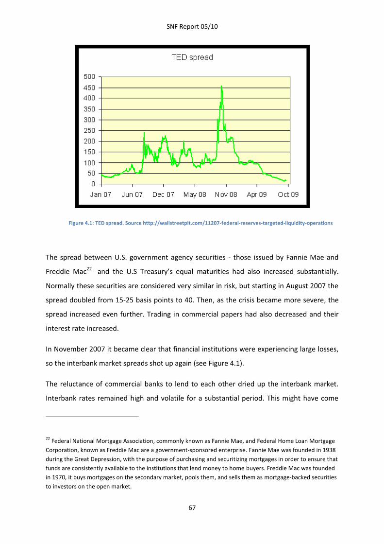
SNF Report 05/10
67
Figure 4.1: TED spread. Source http://wallstreetpit.com/11207-federal-reserves-targeted-liquidity-operations
The spread between U.S. government agency securities - those issued by Fannie Mae and
Freddie Mac22- and the U.S Treasury’s equal maturities had also increased substantially.
Normally these securities are considered very similar in risk, but starting in August 2007 the
spread doubled from 15-25 basis points to 40. Then, as the crisis became more severe, the
spread increased even further. Trading in commercial papers had also decreased and their
interest rate increased.
In November 2007 it became clear that financial institutions were experiencing large losses,
so the interbank market spreads shot up again (see Figure 4.1).
The reluctance of commercial banks to lend to each other dried up the interbank market.
Interbank rates remained high and volatile for a substantial period. This might have come
22 Federal National Mortgage Association, commonly known as Fannie Mae, and Federal Home Loan Mortgage
Corporation, known as Freddie Mac are a government-sponsored enterprise. Fannie Mae was founded in 1938
during the Great Depression, with the purpose of purchasing and securitizing mortgages in order to ensure that
funds are consistently available to the institutions that lend money to home buyers. Freddie Mac was founded
in 1970, it buys mortgages on the secondary market, pools them, and sells them as mortgage-backed securities
to investors on the open market.
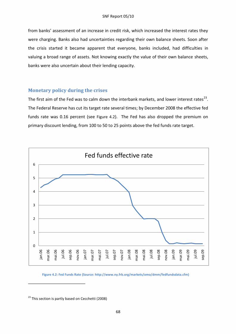
SNF Report 05/10
68
from banks’ assessment of an increase in credit risk, which increased the interest rates they
were charging. Banks also had uncertainties regarding their own balance sheets. Soon after
the crisis started it became apparent that everyone, banks included, had difficulties in
valuing a broad range of assets. Not knowing exactly the value of their own balance sheets,
banks were also uncertain about their lending capacity.
Monetary policy during the crises
The first aim of the Fed was to calm down the interbank markets, and lower interest rates23.
The Federal Reserve has cut its target rate several times; by December 2008 the effective fed
funds rate was 0.16 percent (see Figure 4.2). The Fed has also dropped the premium on
primary discount lending, from 100 to 50 to 25 points above the fed funds rate target.
Figure 4.2: Fed Funds Rate (Source: http://www.ny.frb.org/markets/omo/dmm/fedfundsdata.cfm)
23 This section is partly based on Cecchetti (2008)
0
1
2
3
4
5
6
jan
.06
mar
.06
mai
.06
jul.0
6
sep
.06
no
v.0
6
jan
.07
mar
.07
mai
.07
jul.0
7
sep
.07
no
v.0
7
jan
.08
mar
.08
mai
.08
jul.0
8
sep
.08
no
v.0
8
jan
.09
mar
.09
mai
.09
jul.0
9
sep
.09
Fed funds effective rate
SNF Report 05/10
69
In well-functioning financial markets, changes in actual and expected targets for the federal
funds rate are arbitraged through the financial system to affect the cost of credit and the
price of assets. Many factors affect these markets and the relationship between them but,
on balance, the Fed has previously been able to control the federal funds rate to make the
adjustments to financial conditions needed to foster its objectives for prices and
employment.
From the time that the financial market turmoil emerged in August 2007, the relationship
between the federal funds rate and financial conditions, and hence spending, was disrupted,
with any given federal funds rate implying much tighter conditions than usual.
Not only has the Fed reduced the target federal funds rate aggressively, essentially to zero,
but it has also made credit available to institutions and markets in which it had not
previously intervened24. This was necessary on the one hand because the interest rate
basically had reached its zero lower bound. On the other hand it quickly became apparent
that with the traditional ways of introducing liquidity there was no way to guarantee that
liquidity reached those banks that really needed it. The Fed has introduced several new
facilities to provide liquidity to targeted segments of the market.
Term Auction Facility
Since the aggressive discount lending policy did not work, on December 12, 2007 the Fed
announced that it was going to provide liquidity through an auction, the Term Auction
Facility (TAF). This auction is different from borrowing through the discount window in two
important respects, it provides liquidity for longer periods (28 or 84 days depending on the
auction) and, more importantly, it offers anonymity. The idea behind the TAF is to remove
the stigma of borrowing through the discount window.
24 To varying degrees, similar actions have been taken by other central banks around the world.
SNF Report 05/10
70
The TAF does more than merely distribute funding to the banks that need it. In the TAF the
Fed allows banks to use collateral that might otherwise have very little market value. The
Fed offers a price for these collaterals that is usually above the market value. The TAF
provided liquidity to banks who would otherwise find it hard to obtain liquidity, and also
gave banks time to value the assets they had.
There is some evidence that the TAF helped to decrease the spread between the three-
month LIBOR and the three-month Treasury bill rate by decreasing the amount of securities
on the Fed balance sheet and increasing the amount of loans. Yet the evidence is not very
clear. Taylor and Williams (2009) for example argue the opposite, they find no evidence that
the TAF contributed to the decline in the TED spreads. They show that the TED spread
decrease dwell before targeted liquidity operations were introduced. . Christensen, Lopez
and Rudebusch (2009) and McAndrews, Sarkar and Wang (2008) noted that there was an
impact, but it was on the day of the auction announcement. The Fed announced its intention
to make aggressive use of the Term Auction Facility and currency swaps on December 12.
The TED spread peaked at 225 basis points on that day, and fell steadily after the Fed’s
announcement.
Providing international dollar liquidity
One lesson from 2007 is that conventional central bank tools do not always provide liquidity
for those who need it. This problem becomes even more acute when liquidity is needed by
foreign entities.
On December 12, when the Fed announced that it would provide liquidity through the TAF,
it also announced that a swap line was created with the ECB and the Swiss National Bank.
Through this swap line the Fed provided dollar liquidity to the ECB and the Swiss National
Bank, and those in turn provided dollar liquidity to the European banks.
Term Securities Lending Facility
On 11 March, 2008 the Fed announced an extension of its long-standing securities lending
program creating the Term Securities Lending Facility (TSLF).
SNF Report 05/10
71
For many years the Fed has lent Treasury securities to primary dealers on an overnight basis
in case they were short of certain maturities. Since the Fed holds some of nearly every
Treasury issue, they can lend whatever is needed, thereby ensuring that markets function
smoothly.
The new program transformed the existing program in three ways. The TSLF provided
securities not only overnight but on a longer horizon, for up to 28 days. The TSLF also
broadened the set of collaterals accepted quite dramatically, including "AAA/Aaa-rated
private-label residential [mortgage-backed securities] not on review for downgrade."25
Finally, the Fed announced its willingness to loan up to $200 billion through the TSLF.
Like the TAF, the TSLF has changed the composition of the Fed balance sheet without
changing its aggregate size. The Fed is selling Treasury securities and buying mortgage-
backed securities. The aim is to decrease the spread between these two asset classes.
Fleming, Hrung, Keane, and McAndrews (2008) estimate that the program was immediately
successful.
Bear Stearns
On Friday 14 March 2008 the Federal Reserve Bank of New York gave a loan to Bear Stearns.
Data released on 20 March, combined with press coverage report that the loan was repaid
on 17 March. This was an unconventional action, since Bear Sterns was not a commercial
bank. It was not regulated by the Fed and could not officially borrow from the Fed. The Fed
had to use Article 13.3 of the Federal Reserve Act that gives the Board of Governors the
power to authorize the Federal Reserve Banks to provide loans to any individual,
partnership, or corporation provided that the borrower is unable to obtain credit from a
banking institution.
This was also an unconventional action because the Fed had not issued loans based on
Article 13.3 since the 1930s. Yet, after determining that the failure of Bear Stearns would put
25 See the announcement at www.ny.frb.org/newsevents/news/markets/ 2008/rp080311.html
SNF Report 05/10
72
the whole financial system at risk, the Fed did provide a loan. After the loan, the Fed officials
brokered a deal with JP Morgan Chase to purchase Bear Sterns, with a promise of a $29
billion loan from the Federal Reserve Bank of New York.
In the spring of 2008 around the time of the Bear Stearns problems, the TED spread
exhibited a similar spike (see Figure 4.1). The TED spread peaked at 200 basis points on
March 19. Christensen, Lopez and Rudebusch (2009) chose March 24, the date of Bear
Stearns’ rescue, as the key turning point, after which risk spreads became significantly lower
than their model predicts that they would otherwise have been.
Primary Dealer Credit Facility
The Fed announced its new Primary Dealer Credit Facility on March 16 2008 and also
significantly expanded its repo positions and Term Auction Credit over the next several
weeks.
When creating the Primary Dealer Credit Facility the Federal Reserve used its Article 13(3)
powers for a second time in three days. The 19 primary dealers authorized to participate in
daily open market operations are not investment banks and brokers, so they could not
borrow directly from the Fed. Through the Primary Dealer Credit Facility, however, they
became eligible to borrow from the Federal Reserve.
The PCDF is a collaterized loan facility, which allows for a broad set of collaterals including
“investment-grade corporate securities, municipal securities, mortgage-backed securities
and asset-backed securities for which a price is available”26. One aim of the PCDF was to
provide liquidity to investment banks that now had direct borrowing access. This, in practice,
meant an extension of the lender of last resort function of the Fed to investment banks. A
second aim was to reduce the spread on the assets that were eligible as collaterals for a
FCDF borrowing. The idea is that since the Fed now accepts these assets at any time, it
26 See www.ny.frb.org/newsevents/news/markets/2008/rp080316.html.
SNF Report 05/10
73
should provide a safe demand for these, and they should be readily accepted as collateral in
private borrowing too.
After the failure of Lehman - the Fed’s new Alphabet soup
After Lehman Brothers Holdings Inc. filed for bankruptcy on September 15, 2008, the TED
spread skyrocketed (see Figure 4.1). Targeted Fed liquidity operations increased by $691
billion between September 3 and October 8, despite which the TED spread rose from 114 to
385 basis points and would continue to rise until peaking at 458 basis points on October 10.
By November 12 nonstandard Fed assets had expanded by $1,312 billion.
The Fed has also introduced several new liquidity facilities. The number of acronyms for
these programs started increasing so much that the press often referred to the new facilities
as new additions to the Fed’s alphabet soup.
On September 19, 2008 the Fed introduced the Asset-Backed Commercial Paper Money
Market Mutual Fund Liquidity Facility (AMLF). The aim was to provide liquidity to mutual
funds27. In normal circumstances mutual funds fulfill their redemption requests by selling
their commercial papers. After the bankruptcy of Lehman there was an exodus from these
funds, and selling their commercial papers became more and more difficult. “The Asset-
Backed Commercial Paper Money Market Mutual Fund Liquidity Facility is a lending facility
that provides funding to U.S. depository institutions and bank holding companies to finance
their purchases of high-quality asset-backed commercial papers (ABCP) from money market
mutual funds under certain conditions. The program is intended to assist money funds that
hold such papers in meeting demands for redemptions by investors and to foster liquidity in
the ABCP market and money markets more generally.”28
On October 7th 2008 the Federal Reserve Board announced the creation of the Commercial
Paper Funding Facility (CPFF), a facility that complements the Federal Reserve's existing
27 Mutual funds pool together investors and invest in stocks, bonds and short-term money market instruments
and other securities.
28 http://www.federalreserve.gov/monetarypolicy/abcpmmmf.htm
SNF Report 05/10
74
credit facilities to help provide liquidity to term funding markets. CPFF was targeted
primarily at issuers of commercial papers and intended to improve market conditions for
businesses that rely on the commercial paper market to finance themselves.
Money Market Investor Funding Facility (MMIFF) was announced on October 21, 2008.
MMIFF is aimed to help mutual funds meet their redemptions, just like the AMLF. It differs
from the AMLF primarily because it is targeted at purchasing a broader set of assets,
including unsecured commercial papers. The MMIFF differs from the CPFF in that it aims to
help money market funds rather than issuers of commercial papers.
On November 25, 2008 the Fed went even further and announced plans to provide liquidity
for consumer and small business loans by creating the Term Asset-Backed Securities Loan
Facility (TALF). Starting on March 17 2009, the Fed is offering loans to large investors to buy
newly issued Asset Backed Securities. On March 3, the Fed announced that “Federal Reserve
Bank of New York will lend up to $200 billion to eligible owners of certain AAA-rated ABS
backed by newly and recently originated auto loans, credit card loans, student loans, and
SBA-guaranteed small business loans.”29
These new facilities are still in place. On February 3, 2009 the Fed announced the extension
through October 30, 2009, of its existing liquidity programs that were initially scheduled to
expire on April 30, 2009.
Conclusion
By early 2007 house prices had increased to unprecedented levels, households became
highly leveraged, mortgage quality had declined and asset-backed securitization had become
widespread also internationally. In August 2007 the financial system started to crack, house
prices fell and it became apparent that the quality of mortgage debt was not as high as
previously rated. The loss on balance sheet of banks was hard to value, and liquidity dried up
in the interbank market.
29 http://www.federalreserve.gov/monetarypolicy/20090303a.htm
SNF Report 05/10
75
The Fed first responded with the traditional central bank tools, decreased interest rates and
made borrowing through the discount window cheaper. Yet, it soon became apparent that
these tools did not work, and the Fed had to improvise to get liquidity to market participants
who were in need. New monetary policy tools were introduced, that intended not only to
introduce liquidity, but to introduce liquidity in a directed way to market participants who
were in need. The Fed started following what James D Hamilton calls “monetary policy using
the asset side of the Fed’s balance sheet”. On the asset side the Fed replaced its traditional
holdings of Treasury securities with a variety of new lending programs and alternative
assets.
These new tools were aiming to maintain financial stability in the economy, which is a
function beyond the traditional central bank role. It is an open question how the
responsibility of central banks will change in the future.
Along the way, the Fed has also cooperated internationally with other central banks to
provide enough dollar liquidity to the international banking system. Other central banks
faced similar disruptions in their financial markets and have implemented new facilities in a
similar fashion to the Federal Reserve.
SNF Report 05/10
76
Part II: Macroeconomic Research
Related to Financial Crises
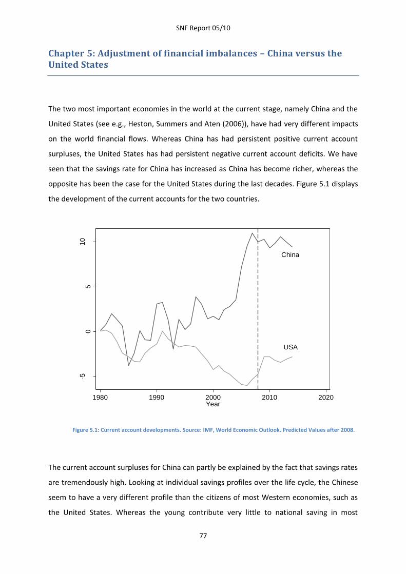
SNF Report 05/10
77
Chapter 5: Adjustment of financial imbalances – China versus the United States
The two most important economies in the world at the current stage, namely China and the
United States (see e.g., Heston, Summers and Aten (2006)), have had very different impacts
on the world financial flows. Whereas China has had persistent positive current account
surpluses, the United States has had persistent negative current account deficits. We have
seen that the savings rate for China has increased as China has become richer, whereas the
opposite has been the case for the United States during the last decades. Figure 5.1 displays
the development of the current accounts for the two countries.
Figure 5.1: Current account developments. Source: IMF, World Economic Outlook. Predicted Values after 2008.
The current account surpluses for China can partly be explained by the fact that savings rates
are tremendously high. Looking at individual savings profiles over the life cycle, the Chinese
seem to have a very different profile than the citizens of most Western economies, such as
the United States. Whereas the young contribute very little to national saving in most
China
USA
-50
510
Cu
rren
t A
ccou
nt B
ala
nce (
as R
atio o
f G
DP
)
1980 1990 2000 2010 2020Year
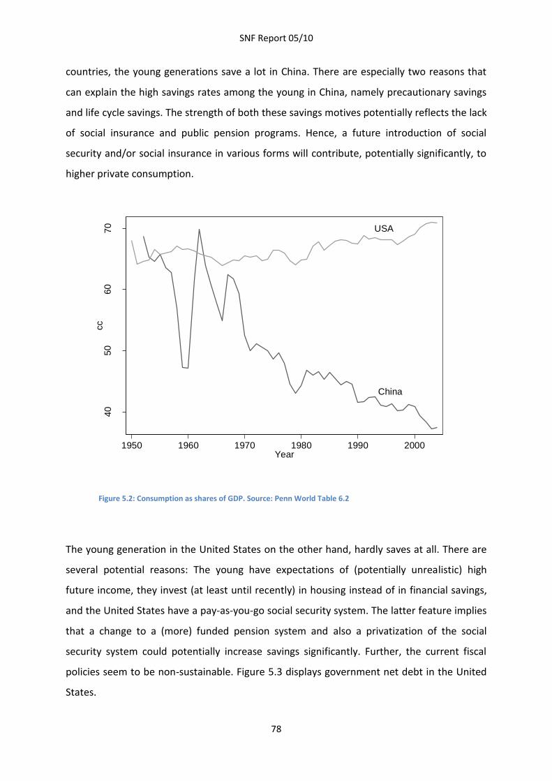
SNF Report 05/10
78
countries, the young generations save a lot in China. There are especially two reasons that
can explain the high savings rates among the young in China, namely precautionary savings
and life cycle savings. The strength of both these savings motives potentially reflects the lack
of social insurance and public pension programs. Hence, a future introduction of social
security and/or social insurance in various forms will contribute, potentially significantly, to
higher private consumption.
Figure 5.2: Consumption as shares of GDP. Source: Penn World Table 6.2
The young generation in the United States on the other hand, hardly saves at all. There are
several potential reasons: The young have expectations of (potentially unrealistic) high
future income, they invest (at least until recently) in housing instead of in financial savings,
and the United States have a pay-as-you-go social security system. The latter feature implies
that a change to a (more) funded pension system and also a privatization of the social
security system could potentially increase savings significantly. Further, the current fiscal
policies seem to be non-sustainable. Figure 5.3 displays government net debt in the United
States.
China
USA
40
50
60
70
cc
1950 1960 1970 1980 1990 2000Year
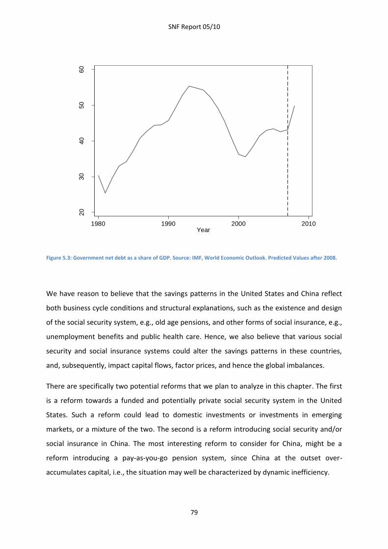
SNF Report 05/10
79
Figure 5.3: Government net debt as a share of GDP. Source: IMF, World Economic Outlook. Predicted Values after 2008.
We have reason to believe that the savings patterns in the United States and China reflect
both business cycle conditions and structural explanations, such as the existence and design
of the social security system, e.g., old age pensions, and other forms of social insurance, e.g.,
unemployment benefits and public health care. Hence, we also believe that various social
security and social insurance systems could alter the savings patterns in these countries,
and, subsequently, impact capital flows, factor prices, and hence the global imbalances.
There are specifically two potential reforms that we plan to analyze in this chapter. The first
is a reform towards a funded and potentially private social security system in the United
States. Such a reform could lead to domestic investments or investments in emerging
markets, or a mixture of the two. The second is a reform introducing social security and/or
social insurance in China. The most interesting reform to consider for China, might be a
reform introducing a pay-as-you-go pension system, since China at the outset over-
accumulates capital, i.e., the situation may well be characterized by dynamic inefficiency.
20
30
40
50
60
Ge
ne
ral g
ove
rnm
ent ne
t de
bt
1980 1990 2000 2010Year
SNF Report 05/10
80
We plan to analyze these two reforms by using a general equilibrium model with overlapping
generations. The basic framework is a two-region overlapping generations (OLG) model, in
the tradition of Diamond (1965) and further developed into a multi-region framework by
Persson (1985). In our analysis we plan to provide four extensions. First, a more detailed
model of the life-cycle should be developed, capturing realistic interactions between tax-
transfer schemes and consumption and saving profiles. Second, we plan to introduce a
realistic demographic structure, simulated by information on the demographic structure in
the two countries. Third, we want to introduce a two-sector production structure with one
tradable good and one non-tradable good. Fourth, we plan to introduce idiosyncratic income
risks.
Introducing these types of features, we will build on the large literature on computable
overlapping generations models, see Fehr and Thøgersen (2009: section 3) for a survey.
Focusing mainly on the interlinkages between China and the US, and the overall effects on
“global financial imbalances”, we will particularly focus on extensions of the somewhat less
developed literature on multi-region versions of this kind of models, see for example Fehr et
al (2007) and Börsch-Supan et al. (2006).
SNF Report 05/10
81
Chapter 6: Determinants of Financial Crises: Jointness and the Role of Expectations
This project will investigate empirically the determinants of financial crises, banking,
currency, twin and debt crises, as discussed in chapter 3. The project will focus on two
questions: First, to what extend is there dependence or jointness among determinants of
financial crises? Second, what role do expectations have in predicting financial crises.
In a recent survey on financial instability, Eichengreen (2004) observes that “*r+ecent
empirical studies suggest that explanations for financial vulnerability are complementary
rather than competing and that they interact in mutually reinforcing ways.” This project will
apply a novel method recently developed by Doppelhofer and Weeks (2009) to investigate
dependence among determinants of financial crises. By looking beyond marginal measures
of variable importance, jointness reveals generally unknown forms of dependence.
Conceptually, one can think of two forms of dependence or jointness: Positive jointness
implies that regressors are complements, representing distinct, but mutually reinforcing
effects. Negative jointness implies that explanatory variables are substitutes and capture
similar underlying effects. The case of complementary determinants of financial crises could
be of particular interest to economists and policymakers. In this case, individual
determinants of financial crises interact and reinforce the effect of one another, thereby
increasing the probability of experiencing a financial crises. As discussed in chapter 3, a
combination of different forms of financial crises, so called twin crises, have particularly
severe economic costs, as illustrated by the recent example of the crisis in Iceland.
The second part of the project assesses the role of expectations quantitatively. We augment
data on determinants of financial crises by a set with private expectations to examine the
predictive power of expectations in the past currency and exchange rate crises. Expectations
of many economic and financial variables are likely to contain information that can be used
to predict financial crises.
SNF Report 05/10
82
Chapter 7: Financial Frictions and Business Cycles
A fundamental and unresolved problem in the business cycle literature is to understand how
shocks to various sectors of the economy are amplified and propagated to have a systematic
impact on key macro aggregates and welfare. The state of the art business cycle literature,
whether of the RBC or DSGE strands, have made significant progress in matching macro
aggregates’ behavior in response to diffusely specified or catch-all type shocks, such as total
factor productivity shocks in the RBC literature. However, the literature has little to say
about what these shocks actually are or what causes them.
At least since Fisher’s (1933) theory of debt deflation as a cause and/or magnifier of the
great depression, economists have been interested in understanding how financial market
imperfections impact economic fluctuations. However, neither the classical Keynesian
approach that dominated macroeconomics for much of the 20th century, nor the RBC and
DSGE models that have become the workhorses of modern macroeconomics, have given any
prominence to financial factors as causes or amplifiers of economic fluctuations. Following
the Modigliani-Miller theorem macroeconomists viewed financial factors only as a veil over
real activity.
Since the seminal contributions of Bernanke and Gertler (1989), Bernanke, Gertler and
Gilchrist (1999) and Kiyotaki and Moore (1997), and in light of the recent crises there has
been a renewed interest among macroeconomists in understanding what impact financial
factors have on economic fluctuations, and in incorporating these factors in state of the art
macroeconomic models. The underlying economic arguments in the models mentioned
above are appealing at an intuitive level; financial constraints on investment in production
factors contribute to magnifying small shocks into large scale aggregate fluctuations.
However, the quantitative effects of these models have in general been found rather small
(see e.g. Chari, Kehoe and McGrattan, 2007) and their impact on modern macroeconomic
models developed for e.g. central bank policy analysis has been limited.
We lack macroeconomic models with financial frictions that are able to produce convincing
answers and reasonable economic stories along the following three dimensions:
SNF Report 05/10
83
1. significant and reasonable quantitative impacts on real and financial variables;
2. a plausible model specification;
3. a transparent transmission mechanism between the real and financial sectors of the
economy.
Although some researchers argue against the ability of modern macroeconomic models to
cope with the difficulties associated with incorporating financial market imperfections, these
frictions could be introduced with relatively modest modifications of the current literature.
Bear in mind that modern dynamic general equilibrium models can produce environments
where the Modigliani-Miller theorem does not hold; defaults occur along the equilibrium
path; there is a role for non-trivial financial intermediation; and, there are multiple interest
rates and credit spreads.
In addition these models provide a laboratory where we can see how they measure up to
real and financial business cycle data and an environment where the dynamic interactions
between agents and policy over time can be analyzed.
Hence modern dynamic general equilibrium models do, in my opinion, provide the best
framework available to analyze the impact that financial market imperfections have on
aggregate fluctuations and what the macroeconomic policy implications of the financial
market imperfections are.
In light of the lack of a clear quantitative impact in the first generation macroeconomic
models with financial frictions, two potential areas of research seem especially promising:
First, the role of a heterogeneous balance sheet constrained corporate sector. The literature
has so far focused on using a representative balance sheet constrained firm. However, as
documented by e.g. Covas and den Haan (2008), there is significant heterogeneity in the US
data on firms’ potential balance sheet constraints.
The largest US firms are least likely to be balance sheet constrained. They also dominate the
aggregate data to such a degree that it is hard to detect significant financial constraints in
the aggregate data. As documented by Chari, Kehoe and Christiano (2008), in the aggregate,
US non-financial firms can actually finance new investment by retained earnings and
dividends alone.
SNF Report 05/10
84
However, smaller firms are far more likely to be balance sheet constrained. Smaller firms are
also important drivers of job creation in the US. Hence it seems reasonable to research
whether macroeconomic models with firms with differing likelihood of being financially
constrained can perform better along the three dimensions set out abroad than the first
generation macroeconomic models with financial frictions.
Second, the role of a balance sheet constrained financial sector. The literature on financial
frictions in macroeconomics has generally focused on a balance sheet constrained corporate
sector. However, as the recent crisis has shown, the financial sector may also become
constrained in its ability to raise external finance.
Few papers have been developed along these lines; notable exceptions are Goodfriend and
McCallum (2007), Gertler and Karadi (2009) and De Walque et al. (2009). As in the literature
on a balance sheet constrained corporate sector, heterogeneity across financial
intermediaries should play a major role in any meaningful analysis of a balance sheet
constrained financial sector.
Developing macroeconomic models with a balance sheet constrained financial sector will
allow us to analyze macro prudential policy for financial stability within a unified framework
that is not available today. However, given the complexity involved in modeling the financial
sector, it is essential to focus on a few key issues in order to achieve a manageable
macroeconomic model. It seems particularly important to understand how balance sheet
constraints on some intermediaries in a heterogeneous financial sector can lead to systemic
dry up of financial lending through contagion and the effects such events have on economic
fluctuations. This is where I plan to focus my effort.
Reasonable macroeconomic models that incorporate financial frictions should be able to
match key features of both real and financial data. Along the real economic dimension the
model should match the amplification and persistence in output and investment in response
to primitive shocks and the positive comovement among the macro aggregates; labor
supply, output, investment and consumption. Along the financial dimension the model
should match credit spread behavior in the data, and the interpretation of credit spreads in
the model should be clearly tied to the risk of default. In addition leverage should play a key
SNF Report 05/10
85
role in determining how hard the financial constraints bite; i.e. the effects of the financial
frictions should be increasing in the leverage ratio of the constrained sector.
SNF Report 05/10
86
Chapter 8: Sectoral allocation and endogenous political preferences
In Norway as well as in other European welfare states, the overall sectoral allocation of
individuals shows one particularly clear trend. The share of individuals (out of the total
number of citizens aged 18 and above) supplying labor to market-exposed private business
sectors is declining, while the share allocated to “the public sphere” broadly defined as
employment in the public sector, in the education system or in some sort of welfare scheme
(old age pensions or other schemes) is increasing.
As discussed in more detail by Thøgersen and Aarbu (2007), there are several explanations
to this development. These include the direct and indirect effects of: i) ageing populations,
automatically increasing the share of individuals receiving old age pensions, ii) the
interaction of generous economic incentives and potentially deteriorating social norms,
leading to an increasing number of exits from the labor force and into disability and other
welfare schemes, and iii) economic growth in general, stimulating reallocation of labor from
capital intensive private business sectors and into labor intensive sectors (including a public
sector that, to a major extent, supplies many income elastic services like schooling and
health care). While some of these explanations hinge on factors that are exogenous to
politics (i.e., ageing population), others are heavily influenced by political choices (i.e.,
incentives of tax-transfer programs and the size and scope of the public sector).
Figure 8.1 shows the development of the sectoral allocation of adult Norwegian individuals
during the period 1978 – 2004. While the median voter during the 1970s was clearly an
employee in a private company, this changed during the 1980s, and during the recent years
the medium voter is clearly in the public sphere.
The tendency discussed above raises an important research question. To what extent will
the described developments in sectoral allocation feed back to the political preferences of
the voters and, in turn, how will that impact the political landscape and the electoral
platforms of the different political parties?
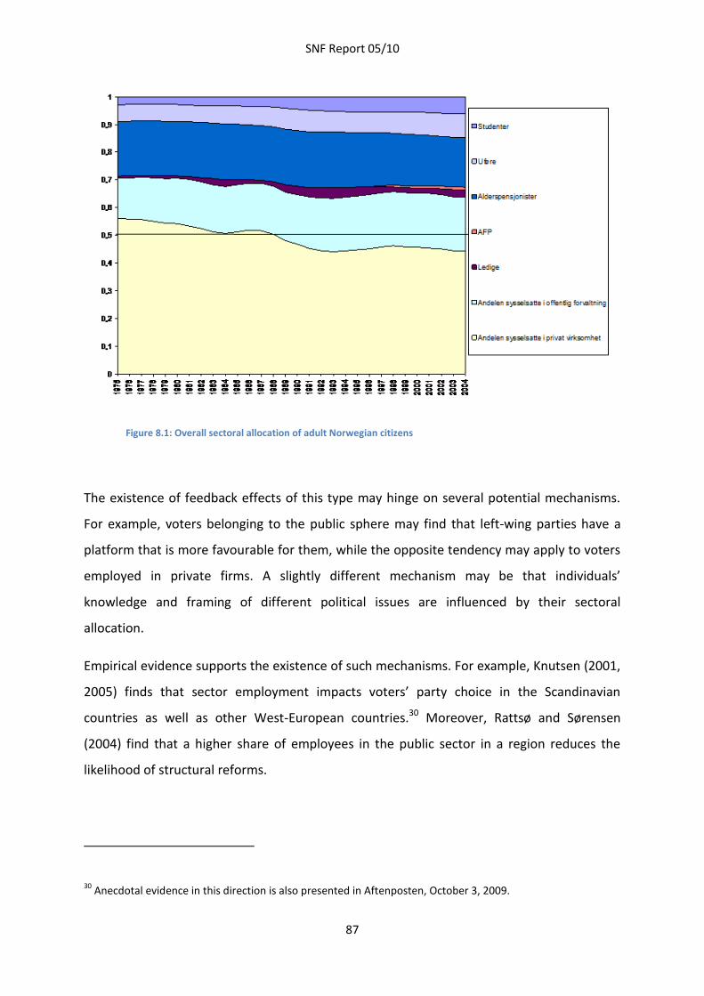
SNF Report 05/10
87
Figure 8.1: Overall sectoral allocation of adult Norwegian citizens
The existence of feedback effects of this type may hinge on several potential mechanisms.
For example, voters belonging to the public sphere may find that left-wing parties have a
platform that is more favourable for them, while the opposite tendency may apply to voters
employed in private firms. A slightly different mechanism may be that individuals’
knowledge and framing of different political issues are influenced by their sectoral
allocation.
Empirical evidence supports the existence of such mechanisms. For example, Knutsen (2001,
2005) finds that sector employment impacts voters’ party choice in the Scandinavian
countries as well as other West-European countries.30 Moreover, Rattsø and Sørensen
(2004) find that a higher share of employees in the public sector in a region reduces the
likelihood of structural reforms.
30 Anecdotal evidence in this direction is also presented in Aftenposten, October 3, 2009.
SNF Report 05/10
88
This part of the project will suggest a theoretical model that captures: (1) a potential causal
link between the political landscape and sectoral allocation, and, in turn, (2) the feedback
from sectoral allocation to political preferences of the voters. We will also attempt to
provide empirical evidence of the alternative mechanisms that come into play.
We will extend a recent paper by Matsen and Thøgersen (2009). They present a probabilistic
voting model where voters’ preferences for alternative public goods display habit formation.
Current policies impact the habit levels for various public goods and services, and in turn the
future preferences of the voters. This implies that the incumbent can influence the
probability of re-election, and this link can be used strategically. As compared to a
benchmark case of a certain re-election, it turns out that a forward-looking, outcome-
oriented government will indeed choose a more polarized allocation between the alternative
public priorities in order to increase the probability of re-election.
Cassing and Hillman (1986) also provide a related framework. They consider the interaction
between the size of an industry and the political support it receives in terms of protection,
for example by means of tariff policy. The current level of protection influences the size of
the industry. In the next stage, this feeds back on political preferences because changes in
industry size alter the political gains and costs of a given level of protection.
SNF Report 05/10
89
References
Altunbas, Yener, Leonardo Gambacorta and David Marqués (2007):”Securitization and the bank
lending channel,” Working Paper Series 838, European Central Bank
Bernanke, B.S. (2005): ”The global saving glut and the US current account deficit.” BIS Review,
16/2005.
Bernanke, B. and M. Gertler (1989): “Agency Cost, Net Worth, and Business Fluctuations.” American
Economic Review, 79, 14-31.
Bernanke, B. (1983): “Nonmonetary effects of the financial crisis in the propagation of the Great
Depression.” American Economic Review 73, 257-276.
Bernanke, B., M. Gertler, and S. Gilchrist (1999): “The Financial Accelerator in a Quantitative Business
Framework.” Handbook of Macroeconomics, 1341-1393.
Bertola, G. and A. Drazen (1993): “Trigger points and budget cuts: Explaining the effects of fiscal
austerity.” American Economic Review, 83, 11-26.
Blinder, A.S. and R. Reis (2005): ”Understanding the Greenspan standard.” Working paper no. 88,
Princeton University.
Bordo, Michael, Barry Eichengreen, Daniela Klingebiel, and Maria Soledad Martinez-Peria (2001). “Is
the Crisis problem Growing More Severe?” Economic Policy 16.
Bordo, M.D. and J.G. Haubrich (2009): “Credit crises, money and contractions: An historical view.”
NBER Working Paper no. 15389.
Bordo, M.D. and C.M. Meissner (2006): “Financial Crises and Foreign Currency Debt: 1880-1913 vs.
1972-1997”, Journal of Banking and Finance, 60, 3299-3329.
Börsch-Supan, A., A. Ludwig, and J. Winter (2006): “Ageing, pension reform and capital flows: A
multi-country simulation model”, Economica, 73, 625-658.
Brunnermeier, Markus (2008): “Bubbles.” In Steven N. Durlauf and Lawrence E. Blume (eds.) The
New Palgrave Dictionary of Economics. Second Edition.
Burns, A.F. and W.C. Mitchell (1946): “Measuring business cycles.” National Bureau of Economic
Research, New York.
Burnside, Craig, Martin Eichenbaum and Sergio Rebelo (2008): “Currency Crises Models.” In Steven
N. Durlauf and Lawrence E. Blume (eds.) The New Plgrave Dictionary of Economics. Second Edition.
Cagan, P. (1965): Determinants and effects of changes in the stock of money 1875-1960. Columbia
University Press, New York.
Calomiris, Charles W. (2008): “Banking Crises.” In Steven N. Durlauf and Lawrence E. Blume (eds.)
The New Plgrave Dictionary of Economics. Second Edition.

SNF Report 05/10
90
Case, Karl E., John M. Quigley, Robert J. Shiller (2005): "Comparing Wealth Effects: The Stock Market
versus The Housing Market," Advances in Macroeconomics, vol.5 no.1
Cassing, J.H. and A.L. Hillman (1986): “Shifting comparative advantage and senescent industry
collapse”, American Economic Review, 76, 516-523.
Cecchetti, Stephen G. (2008): “Crisis and Responses: The Federal Reserve in the Early Stages of the
Financial Crisis.” Journal of Economic Perspectives, 23(1): 51-75.
Chari, V.V., Patrick J. Kehoe, and Ellen R. McGrattan (2007): “Business Cycle Accounting.”
Econometrica, 75(3): 781-836.
Chari, V.V., Lawrence Christiano, and Patrick Kehoe (2008), “Facts and Myths about the Financial
Crisis of 2008. ” Federal Reserve Bank of Minneapolis, Working Paper 666.
Covas and W. den Haan (2008), “The Role of Debt and Equity Finance over the Business Cycle.”
Working paper.
De Walque, G., O. Pierrard, and A. Rouabah (2009): Financial (In)Stability, Supervision and Liquidity
Injection: a Dynamic General Equilibrium Framework.” Working paper.
Diamond, P.A. (1965): “National Debt in a Neoclassical Growth Model”, American Economic Review,
55: 1126-1150.
Doppelhofer, G and M. Weeks (2009): „Jointness of Growth Determinants.” Journal of Applied
Econometrics 24: 209-244.
Eichengreen, B. and J. Sachs (1985): “Exchange rates and economic recovery in the 1930s.” Journal of
Economic History 45, 925-946.
Fehr, H., S. Jokisch and L.J. Kotlikoff (2007): “Will China eat our lunch or take us to dinner? --
Simulating the transition paths of the U.S., EU, Japan, and China”, in: T. Ito und A. Rose (eds.), Fiscal
Policy and Management, East Asia Seminar on Economics Volume 16, University of Chicago Press,
Chicago.
Fehr, H. and Ø. Thøgersen (2009): “Social security and future generations”, In: Robert J. Brent (ed.),
Handbook on Research in Cost-Benefit Analysis, Edward Elgar Publishers, ch. 16, 417-454.
Fisher, I. (1933): “The Debt-Deflation Theory of Great Depressions.” Econometrica, 1, 337-357.
Fleming, Michael, Warren Hrung, Frank Keane, and James McAndrews (2008): “Repo Market Effects
of the TSLF,” Current Issues in Economics and Finance, Federal Reserve Bank of New York.
Friedman, M. and A.J. Schwartz (1963): A Monetary History of the United States. Princeton University
Press, Princeton.
Gavin, W.T. (2009): “More money: Understanding recent changes in the monetary base.” Federal
Reserve Bank of St. Louis Review, March/April, 49-59.
Gertler, M. and P. Karadi (2009): “A Model of Unconventional Monetary Policy.” Working Paper.
SNF Report 05/10
91
Goodfriend, M. and B.T. McCallum (2007), “Banking and Interest Rates in Monetary Policy Analysis: A
Quantitative Exploration.” Journal of Monetary Economics, 54.
Heston, A. Summers, R., and Aten, B (2006): Penn World Table Version 6.2, Center for International
Comparisons of Production, Income and Prices at the University of Pennsylvania.
http://pwt.econ.upenn.edu/
Honkapohja, Seppo (2008): “The 1990’s Financial Crises in Nordic Countries.” Bank of
Finland.
Kaminsky, Graciela L. and Carmen M. Reinhart (1999): “The Twin Crises: The Causes of Banking and
Balance-of-Payments Problems.” American Economic Review, 89(3): 473-500.
Keister, T. and J. McAndrews (2009): “Why are banks holding so many reserves?” Staff Report no.
380, Federal Reserve Bank of New York.
Kindleberger, Charles P. and Robert Z. Aliber (2005). Manias, Panics and Crashes: A History if
Financial Crises. Palgrave MacMillan.
Kiyotaki, Nobuhiro and John Moore (1997). “Credit Cycles.” Journal of Political Economy, 105, 211-
248.
Klovland, J.T. (1998): “Monetary policy and business cycles in the interwar years: The Scandinavian
experience.” European Review of Economic History 2, 309-344.
Knutsen, K. (2001): “Social class, sector employment and gender as party cleavages in the
Scandinavian countries: A comparative longitudinal study, 1970-95”, Scandinavian Political Studies,
24, 311-350.
Knutsen, K. (2005): “The impact of sector employment on party choice: A comparative study of eight
West European countries”, European Journal of Political Research, 44, 593-621.
Knutsen, S. (2007): Staten og kapitalen i det 20. århundre – Regulering, kriser og endring i det norske
finanssystemet 1900-2005. Ph. D. dissertation, University of Oslo.
Krugman, Paul (1979), 'A model of balance-of-payments crises'. Journal of Money, Credit, and
Banking 11, pp. 311-25.
Matsen, E. og Ø. Thøgersen (2009): ”Habit formation, extremism and debt policy”, Public Choice,
forthcoming.
McAndrews, James, Asani Sarkar, and Zhenyu Wang (2008): "The effect of the Term Auction Facility
on the London Inter-Bank Offered Rate," Staff Reports 335, Federal Reserve Bank of New York.
Minsky, Hyman P. (1982): “The Financial Instability Hypothesis: Capitalistic Processes and the
Behavior of the Economy .” In C.P. Kindleberger and J.-P. Laffargue (eds.) Financial Crises: Theory,
History and Policy. Cambridge University Press.
Mizen, P. (2008): ”The credit crunch of 2007-2008: A discussion of the background, market reactions,
and policy responses.” Federal Reserve Bank of St. Louis Review, September/October, 531-567.
SNF Report 05/10
92
Moe, Thorvald G, Jon A. Solheim, and Bent Vale (eds.) (2004): The Norwegian Banking Crisis. Norges
Bank Occasional Papers , Nr. 33.
Obstfeld, , Maurice (1984): “The Logic of Currency Crises.” Cahiers Economiques et Monétaires, 43,
189-213.
Obstfeld, Maurice and Alan M. Taylor (2004): Global Capital Markets: Integration, Crises, and
Growth. Cambridge University Press.
Persson, T. (1985). “Deficits and intergenerational welfare in open economies”, Journal of
International Economics, 19(1-2): 67-84.
Ranciere, Romain, Aaron Tornell, and Frank Westermann (2008). “Systemic Crises and Growth.”
Quarterly Journal of Economics, February, 359-406.
Rattsø, J. og R.J. Sørensen (2004): ”Public employees as swing voters: Empirical evidence on the
opposition to public reform”, Public Choice, 119, 281-310.
Reinhart, Carmen and Kenneth S. Rogoff (2008a): “Is the 2007 US Sub-Prime Financial Crisis So
Different? An International Historical Comparison.” American Economic Review: Papers &
Proceedings, 98:2, 339-344.
Reinhart, Carmen and Kenneth S. Rogoff (2008b): “Banking Crises: An Equal Opportunity Menace.”
NBER Working Paper, No. 14587.
Reinhart, Carmen and Kenneth S. Rogoff (2009a): This Time is Different: Eight Centuries of Financial
Follies. Princeton University Press.
Reinhart, Carmen and Kenneth S. Rogoff (2009b): “The Aftermath of Financial Crisis.” American
Economic Review, 99(2): 466-472.
Romer, C.D. (1992): “What ended the Great Depression?” Journal of Economic History 52, 757-784.
Romer, C.D. (1994): “Remeasuring business cycles” Journal of Economic History 54, 573-609.
Romer, C.D. (2009): “Lessons from the Great Depression for economic recovery in 2009.” mimeo.
Sinn, Hans-Werner (2009): Risk-Taking, Limited Liability, and the Banking Crisis, Ifo Institute for
Economic Research.
Taylor, John B. and John C. Williams (2009): “A Black Swan in the Money Market,” American
Economic Journal: Macroeconomics, 1(1), 58-83.
Thøgersen, Ø. and K.O. Aarbu (2007): “Sektortilhørighet og politikk.” Økonomisk Forum, 9, 25-37.
Wheelock, D.C. (2009): ”How not to reduce excess reserves.” Economic Synopses, Federal Reserve
Bank of St. Louis, no. 38.
White, E. N. (2009): “Lessons from the Great American Real Estate Boom and Bust of the 1920s”,
NBER Working Paper no 15573.
SNF Report 05/10
93
World Economic Outlook (October 2009): Sustaining the Recovery, Chapter 3, International Monetary
Fund.
SNF Report 05/10
94
PUBLICATIONS WITHIN SNF’S RESEARCH PROGRAMME “CRISIS,
RESTRUCTURING AND GROWTH”
2010- I. Almås Crisis, restructuring and growth: A macroeconomic perspecitve G. Doppelhofer SNF Report No 05/10 J. C. Haatvedt J. T. Klovland K. Molnar Ø. Thøgersen L. B. Lien Recessions across industries: A survey SNF Working Paper No 16/10 K. G. Nyborg Liquidity, ideas and the financial crisis P. Östberg SNF Working Paper No 17/10