i

Report on Approximation of the Gamma Distribution

Submitted to Professor Knight

for English 316

Brigham Young University Provo, Utah 9 April 2014

by Brianne Cass

Trevor Johnson Jane Ostergar

Ammon Washburn

ii

Brianne Cass English 316 Student

9 April 2014 Professor Liz Knight

Dear Professor Knight, We have submitted herewith our technical report that summarizes our findings on the topic of “Approximation of the Gamma Distribution”. This report is not being submitted to any other journal or publisher or professor. This report is for both you as our professor and grader of this report, as well as for our classmates, to whom we will be presenting our research. The purpose of this report is to demonstrate our ability to go through the whole research process as well as our ability to complete a well written technical report. For this report Ammon Washburn will be the correspondence author because he is the most knowledgeable about the subject matter our report is on. He can be contacted by phone at

or by e-mail at . Sincerely, Brianne Cass Trevor Johnson Jane Ostergar Ammon Washburn

iii

TABLE OF CONTENTS LIST OF FIGURES ........................................................................................................................................... iv

LIST OF TABLES .............................................................................................................................................. v

ABSTRACT ..................................................................................................................................................... vi

I. INTRODUCTION ...................................................................................................................................... 1

II. GAMMA DISTRIBUTION ........................................................................................................................ 3

III. SIMPLE SIMPSON’S METHOD ............................................................................................................... 4

Strategy of Method ............................................................................................................................... 4

Derivation of Error for Gamma Distribution ......................................................................................... 7

Appraisal ............................................................................................................................................... 8

IV. COMPOSITE SIMPSON’S METHOD ....................................................................................................... 9

Strategy of Method ............................................................................................................................... 9

Derivation of Composite Error Bound ................................................................................................ 11

V. ADAPTIVE SIMPSON’S METHOD ......................................................................................................... 12

Strategy of Method ............................................................................................................................. 12

Stability ............................................................................................................................................... 14

Derivation of Error Bound................................................................................................................... 14

Appraisal ............................................................................................................................................. 16

VI. TWO-THIRDS SIMPSON’S METHOD ................................................................................................... 16

Strategy of Method ............................................................................................................................. 16

Derivation of Method and Error ......................................................................................................... 18

Appraisal ............................................................................................................................................. 19

VII. COMPARISON.................................................................................................................................... 20

VIII. CONCLUSION.................................................................................................................................... 21

REFERENCES ................................................................................................................................................ 23

APPENDIXES ................................................................................................................................................ 24

iv

LIST OF FIGURES Figure 1: Gamma Distribution ...................................................................................................................... 3 Figure 2: Simple Simpson's .......................................................................................................................... 5 Figure 3: Fourth Derivative .......................................................................................................................... 7 Figure 4: Composite Simpson's .................................................................................................................. 10 Figure 5: Adaptive Simpson's ..................................................................................................................... 13 Figure 6: Two-Thirds Simpson's ................................................................................................................. 17

v

LIST OF TABLES Table 1: Simple Simpson's ............................................................................................................................ 8 Table 2: Composite Simpson's .................................................................................................................... 12 Table 3: Adaptive Simpson's ...................................................................................................................... 16 Table 4: Two-Thirds Simpson's .................................................................................................................. 19 Table 5: Comparison Summary .................................................................................................................. 20

vi

ABSTRACT

In many scenarios, it is useful to integrate the gamma distribution over a given interval in

order to calculate the probability of a certain event occurring, yet there is no known solution to

this particular integral. As such, it is necessary to approximate the integral using some type of

numerical method. An effective approximation provides an accurate estimate, is easy to

implement, and stays theoretically consistent. The goal is to get the estimation close to the real

answer within some tolerance. It is also helpful if the approximation is easily and quickly

calculated on a computer. The various Simpson’s methods that have been developed since

Simpson proposed the original method have proven to be very useful in these regards; however,

there are numerous variations. To goal of our research is to find which variation is the most

efficient for the gamma distribution. We will explore four different Simpson’s methods—simple,

composite, adaptive, and two-thirds—with regard to their theoretical strengths and how well they

approximate sample intervals. From our analysis, we have decided that the composite Simpson’s

method is the most efficient in approximating the real answer. Although it is not the most

accurate approximation, it is relatively easy to implement and does not have a considerably long

computational time. We recommend the composite Simpson’s method as the best way to

evaluate any interval along the gamma distribution.

1

APPROXIMATION OF THE GAMMA DISTRIBUTION

I. INTRODUCTION

“The theory and application of integrals is one of the great and central themes of

mathematics,” said numerical analysts P. Davis and P. Rabinowitz [2]. This report addresses the

problem of how to approximate otherwise unsolvable integrals. The study of these impossible

integrals is called quadrature analysis. There are many integrals that are commonly used that can

only be solved through approximation. There are many known approximation methods which

accurately approximate an integral. Because they are so diverse, some are better than others

when approximating certain functions. One such case is when taking the integral of the gamma

distribution, a common probability density function. We want to approximate this impossible

integral because the area under the function gives us the probability or the likelihood of an event

happening.

We will discover which approximation method is superior in estimating this unknown

integral of the gamma distribution through creating computer programs that implement these

methods that we have chosen to compare. The approximation methods we will compare are the

simple Simpson’s method, composite Simpson’s method, adaptive Simpson’s method, and two-

thirds Simpson’s method. These methods have been widely researched and much is known about

them. In fact, it has been said by Milton Abramowitz, that “95% (sic) of all practical work in

numerical analysis boil[s] down to applications of Simpson’s rule and linear interpolation” [3].

When comparing these different approximation methods we will use two standards of

judgment: the speed and the accuracy of the approximation. The speed will be measured by how

fast the approximation converges and by how fast the computer can run the method. The

2

accuracy will be measured by determining the maximum possible error, or error bound, as well

as running tests to determine the actual error for each of the methods. It should be noted though

that even if one method has a smaller error bound, it does not necessarily imply that the method

will be more accurate [6].

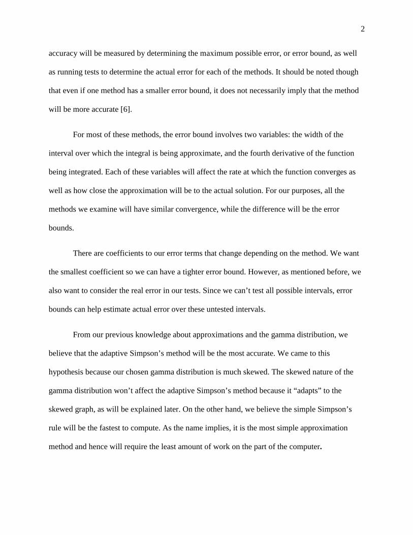
For most of these methods, the error bound involves two variables: the width of the

interval over which the integral is being approximate, and the fourth derivative of the function

being integrated. Each of these variables will affect the rate at which the function converges as

well as how close the approximation will be to the actual solution. For our purposes, all the

methods we examine will have similar convergence, while the difference will be the error

bounds.

There are coefficients to our error terms that change depending on the method. We want

the smallest coefficient so we can have a tighter error bound. However, as mentioned before, we

also want to consider the real error in our tests. Since we can’t test all possible intervals, error

bounds can help estimate actual error over these untested intervals.

From our previous knowledge about approximations and the gamma distribution, we

believe that the adaptive Simpson’s method will be the most accurate. We came to this

hypothesis because our chosen gamma distribution is much skewed. The skewed nature of the

gamma distribution won’t affect the adaptive Simpson’s method because it “adapts” to the

skewed graph, as will be explained later. On the other hand, we believe the simple Simpson’s

rule will be the fastest to compute. As the name implies, it is the most simple approximation

method and hence will require the least amount of work on the part of the computer.

3

II. GAMMA DISTRIBUTION

As previously stated, we decided to study the gamma distribution. The reason for this

decision was that the gamma distribution can be very skewed, or asymmetric, which will really

test the different approximation methods. For this

research we decided to use a specific gamma

distribution to simplify our calculations. The gamma

distribution has two parameters, shape (α) and scale

(β). We chose the value 1.5 for both our shape and

our scale, because using an integer value for these

parameters results in an integral function has an

exact solution. These parameter values change for

each unique situation in which a gamma distribution is used. Figure 1 shown above is a graphical

representation of our specified gamma distribution. Below is, respectively, the general gamma

distributions formula as well as our specific formulaic representation:

The gamma distribution is used most often to predict waiting time, or time until something runs

out; e.g., the amount of time a person has to wait in line, or how long until a light bulb will burn

out. This distribution is applicable to everyday life situations; therefore, being able to

approximate the gamma distribution through a simple approximation computer program will be

very useful to the general public.

(1)

Figure 1: Gamma Distribution

(2)

4

III. SIMPLE SIMPSON’S METHOD

Strategy of Method

Simple Simpson’s method, as the name suggests, is the easiest way to approximate an

integral using the technique Thomas Simpson published in 1743 [7]. This technique involves

approximating a function whose integral is too difficult to accurately calculate with a polynomial

whose integral is more easily solvable. The polynomial that Simpson uses for the approximation

is the parabola.

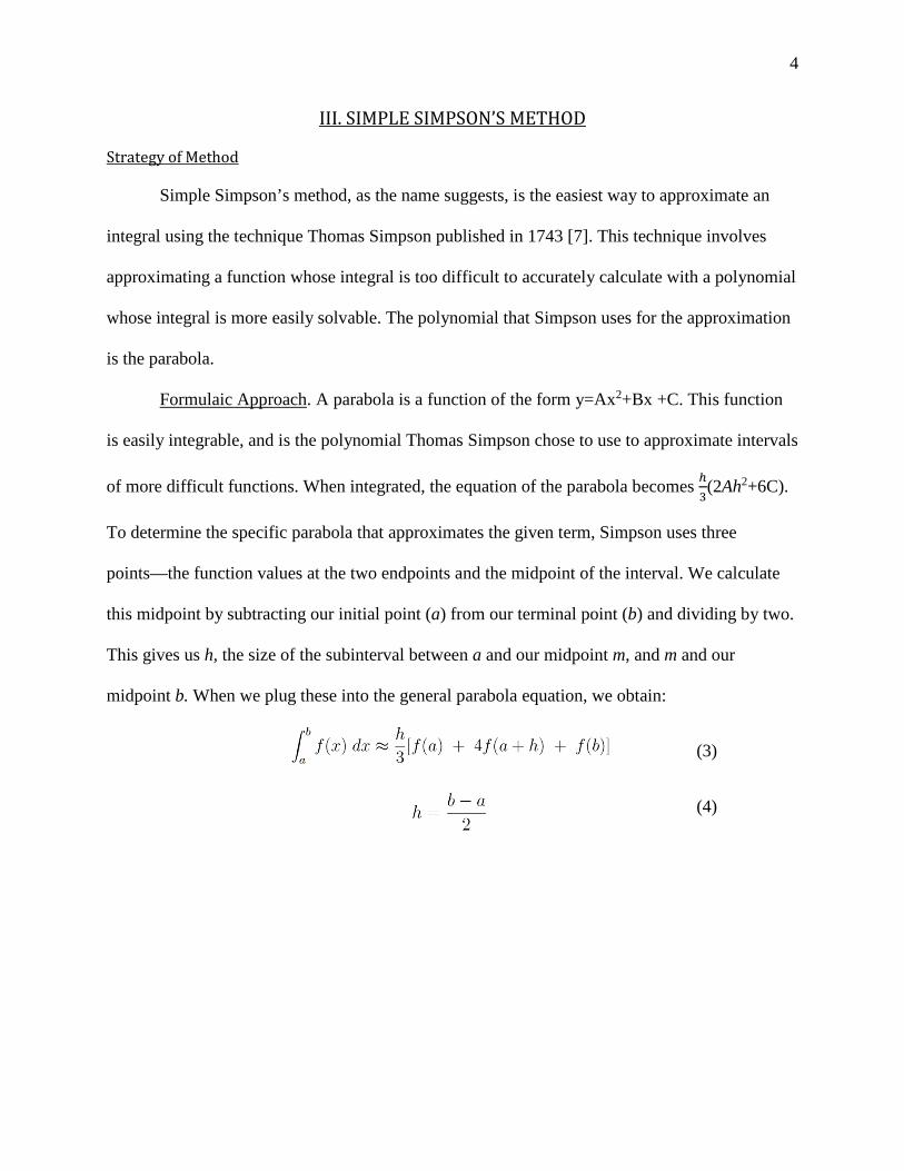
Formulaic Approach. A parabola is a function of the form y=Ax2+Bx +C. This function

is easily integrable, and is the polynomial Thomas Simpson chose to use to approximate intervals

of more difficult functions. When integrated, the equation of the parabola becomes ℎ3(2Ah2+6C).

To determine the specific parabola that approximates the given term, Simpson uses three

points—the function values at the two endpoints and the midpoint of the interval. We calculate

this midpoint by subtracting our initial point (a) from our terminal point (b) and dividing by two.

This gives us h, the size of the subinterval between a and our midpoint m, and m and our

midpoint b. When we plug these into the general parabola equation, we obtain:

(3)

(4)

5

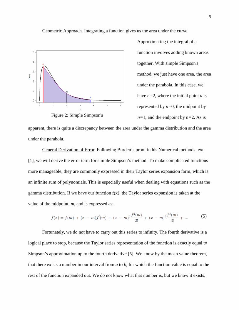
Geometric Approach. Integrating a function gives us the area under the curve.

Approximating the integral of a

function involves adding known areas

together. With simple Simpson's

method, we just have one area, the area

under the parabola. In this case, we

have n=2, where the initial point a is

represented by n=0, the midpoint by

n=1, and the endpoint by n=2. As is

apparent, there is quite a discrepancy between the area under the gamma distribution and the area

under the parabola.

General Derivation of Error. Following Burden’s proof in his Numerical methods text

[1], we will derive the error term for simple Simpson’s method. To make complicated functions

more manageable, they are commonly expressed in their Taylor series expansion form, which is

an infinite sum of polynomials. This is especially useful when dealing with equations such as the

gamma distribution. If we have our function f(x), the Taylor series expansion is taken at the

value of the midpoint, m, and is expressed as:

Fortunately, we do not have to carry out this series to infinity. The fourth derivative is a

logical place to stop, because the Taylor series representation of the function is exactly equal to

Simpson’s approximation up to the fourth derivative [5]. We know by the mean value theorem,

that there exists a number in our interval from a to b, for which the function value is equal to the

rest of the function expanded out. We do not know what that number is, but we know it exists.

Figure 2: Simple Simpson's

(5)

6

Because we do not know the value of this number, this term in the fourth derivative is our error.

We can easily integrate the first four terms of the Taylor Series, but our fourth derivative remains

an unknown. When we integrate the function, we obtain:

Note that when the endpoints of the integral are plugged in, the first derivative and the second

derivative cancel, and the function value and third derivative just become double the length of

the interval, leaving us:

In order to calculate the integral of our unknown error term, we must employ the Weighted Mean

Value Theorem for integrals (see appendix A). In essence, this lets us replace our function with a

constant term which we can easily factor out of the equation and simplify, like so:

To simplify the equation further, it is necessary to use an approximation of the second derivative

(see appendix A), which involves another unknown number ξ in our interval [a,b]. By the

Intermediate Value Theorem, we can represent these two unknown values with a single constant,

leaving us the general equation for simple Simpson’s method:

Note that the last term is our unknown, or our error. It is what makes our method an

approximation. Because it involves the fourth derivative, we know Simple Simpson’s method is

exactly correct for functions of degree three or less.

(6)

(7)

(8)

(9)

7

Derivation of Error for Gamma Distribution

Note that the last term is our unknown, or our error. It is what makes our method an

approximation. Because it involves the fourth derivative, we know Simple Simpson’s method is

exactly correct for functions of degree three or less. Below is the formula for the error where K

represents the maximum value of the fourth derivative of the function within the given interval

[3]:

Using this value for K guarantees that the error bound given is the largest possible error margin.

Therefore, in order to find a maximum possible error when using the simple Simpson’s method,

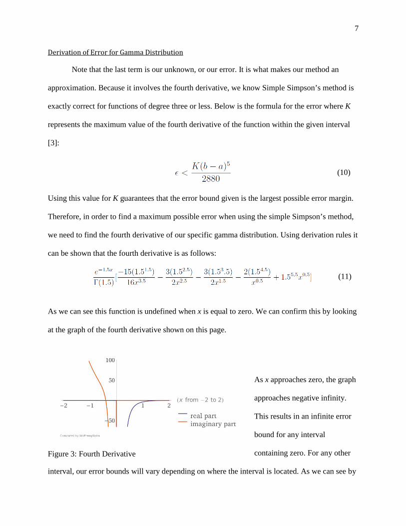
we need to find the fourth derivative of our specific gamma distribution. Using derivation rules it

can be shown that the fourth derivative is as follows:

As we can see this function is undefined when x is equal to zero. We can confirm this by looking

at the graph of the fourth derivative shown on this page.

As x approaches zero, the graph

approaches negative infinity.

This results in an infinite error

bound for any interval

containing zero. For any other

interval, our error bounds will vary depending on where the interval is located. As we can see by

(10)

(11)

Figure 3: Fourth Derivative

8

the graph, we will have our largest error bounds when the interval is close to zero. For these

values, we will have a large maximum absolute value for our fourth derivative thereby creating

larger error bounds.

Appraisal

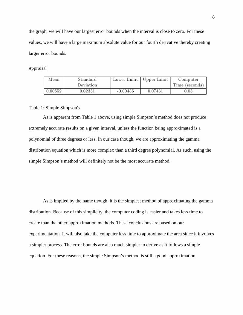
Table 1: Simple Simpson's

As is apparent from Table 1 above, using simple Simpson’s method does not produce

extremely accurate results on a given interval, unless the function being approximated is a

polynomial of three degrees or less. In our case though, we are approximating the gamma

distribution equation which is more complex than a third degree polynomial. As such, using the

simple Simpson’s method will definitely not be the most accurate method.

As is implied by the name though, it is the simplest method of approximating the gamma

distribution. Because of this simplicity, the computer coding is easier and takes less time to

create than the other approximation methods. These conclusions are based on our

experimentation. It will also take the computer less time to approximate the area since it involves

a simpler process. The error bounds are also much simpler to derive as it follows a simple

equation. For these reasons, the simple Simpson’s method is still a good approximation.

9

IV. COMPOSITE SIMPSON’S METHOD

Strategy of Method

Composite Simpson’s method applies simple Simpson’s method multiple times along the

same interval. For simple Simpson’s method, we evaluated the two endpoints and the midpoint.

To increase our accuracy, we can further subdivide the two intervals we initially have with

simple Simpson’s method into many more intervals. This is especially effective because the size

of the intervals decreases in half but our error term decreases exponentially as more intervals are

taken. Because the error term relies on a power of the interval, h, the smaller the interval, the

smaller the error term.

10

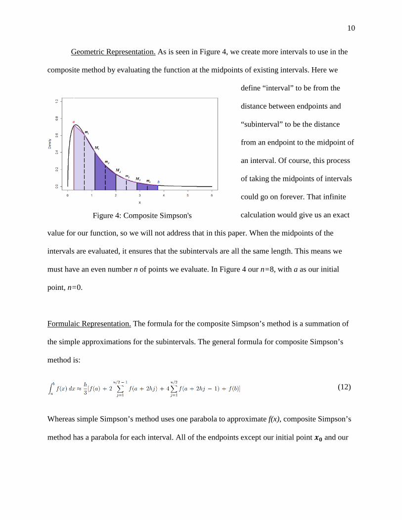
Geometric Representation. As is seen in Figure 4, we create more intervals to use in the

composite method by evaluating the function at the midpoints of existing intervals. Here we

define “interval” to be from the

distance between endpoints and

“subinterval” to be the distance

from an endpoint to the midpoint of

an interval. Of course, this process

of taking the midpoints of intervals

could go on forever. That infinite

calculation would give us an exact

value for our function, so we will not address that in this paper. When the midpoints of the

intervals are evaluated, it ensures that the subintervals are all the same length. This means we

must have an even number n of points we evaluate. In Figure 4 our n=8, with a as our initial

point, n=0.

Formulaic Representation. The formula for the composite Simpson’s method is a summation of

the simple approximations for the subintervals. The general formula for composite Simpson’s

method is:

Whereas simple Simpson’s method uses one parabola to approximate f(x), composite Simpson’s

method has a parabola for each interval. All of the endpoints except our initial point 𝒙𝒙𝟎𝟎 and our

Figure 4: Composite Simpson's

(12)

11

terminal point 𝒙𝒙𝒏𝒏 are used in two different parabolas. As you can see, the formula takes this

repetition into account.

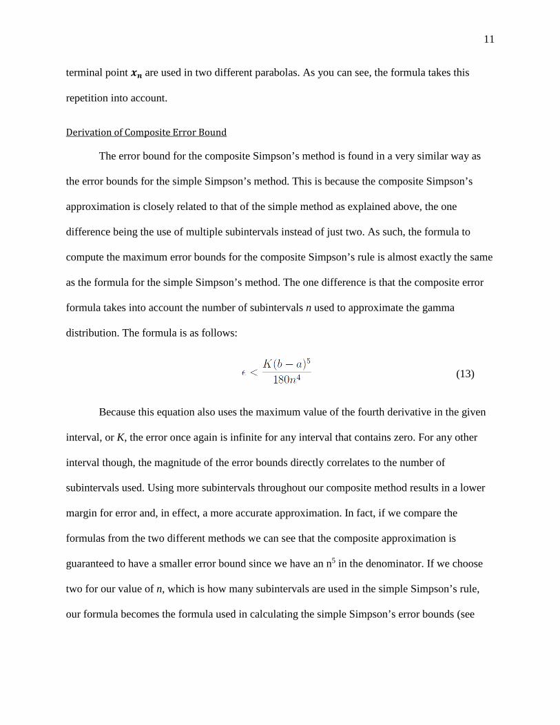
Derivation of Composite Error Bound

The error bound for the composite Simpson’s method is found in a very similar way as

the error bounds for the simple Simpson’s method. This is because the composite Simpson’s

approximation is closely related to that of the simple method as explained above, the one

difference being the use of multiple subintervals instead of just two. As such, the formula to

compute the maximum error bounds for the composite Simpson’s rule is almost exactly the same

as the formula for the simple Simpson’s method. The one difference is that the composite error

formula takes into account the number of subintervals n used to approximate the gamma

distribution. The formula is as follows:

Because this equation also uses the maximum value of the fourth derivative in the given

interval, or K, the error once again is infinite for any interval that contains zero. For any other

interval though, the magnitude of the error bounds directly correlates to the number of

subintervals used. Using more subintervals throughout our composite method results in a lower

margin for error and, in effect, a more accurate approximation. In fact, if we compare the

formulas from the two different methods we can see that the composite approximation is

guaranteed to have a smaller error bound since we have an n5 in the denominator. If we choose

two for our value of n, which is how many subintervals are used in the simple Simpson’s rule,

our formula becomes the formula used in calculating the simple Simpson’s error bounds (see

(13)

12

equation (10)). Therefore, as long we divide our interval into more than two subintervals, our

error bounds will automatically be less for the composite Simpson’s method.

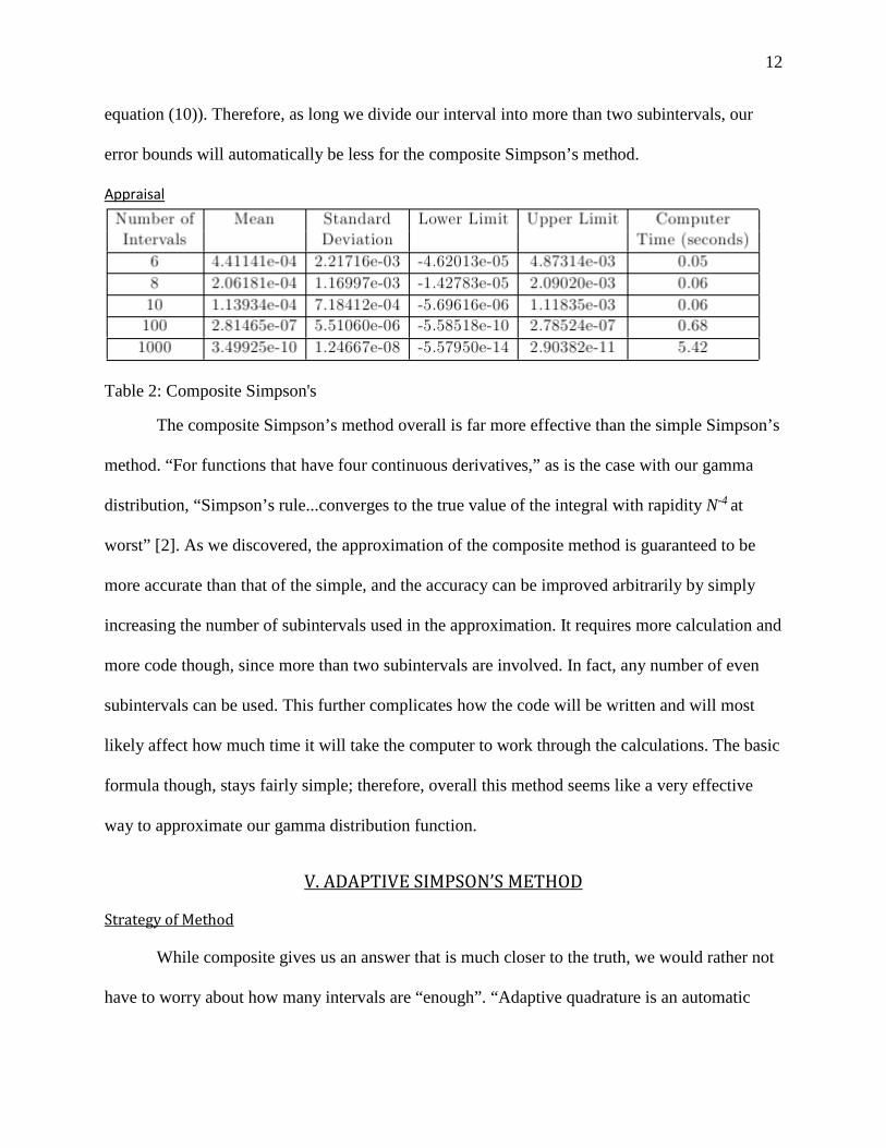
Appraisal

Table 2: Composite Simpson's

The composite Simpson’s method overall is far more effective than the simple Simpson’s

method. “For functions that have four continuous derivatives,” as is the case with our gamma

distribution, “Simpson’s rule...converges to the true value of the integral with rapidity N-4 at

worst” [2]. As we discovered, the approximation of the composite method is guaranteed to be

more accurate than that of the simple, and the accuracy can be improved arbitrarily by simply

increasing the number of subintervals used in the approximation. It requires more calculation and

more code though, since more than two subintervals are involved. In fact, any number of even

subintervals can be used. This further complicates how the code will be written and will most

likely affect how much time it will take the computer to work through the calculations. The basic

formula though, stays fairly simple; therefore, overall this method seems like a very effective

way to approximate our gamma distribution function.

V. ADAPTIVE SIMPSON’S METHOD

Strategy of Method

While composite gives us an answer that is much closer to the truth, we would rather not

have to worry about how many intervals are “enough”. “Adaptive quadrature is an automatic

13

procedure for increasing the accuracy of a numerical approximation to an integral by increasing

the number of samples of the integrand. Additional samples only need to be taken where the

quadrature scheme is having numerical difficulties” [7]. These numerical difficulties are related

to the difference in the answers that simple and composite Simpson’s methods give. Through

some careful manipulation we can see that using composite Simpson’s method with four

subintervals is about 15 times more accurate than simple Simpson’s method (to be derived in a

later section). Taking advantage of this we can simply let a computer decide when to stop

making intervals. Also, if we are careful, we can put more intervals in areas that we need them.

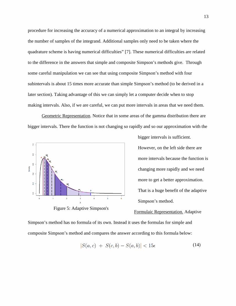
Geometric Representation. Notice that in some areas of the gamma distribution there are

bigger intervals. There the function is not changing so rapidly and so our approximation with the

bigger intervals is sufficient.

However, on the left side there are

more intervals because the function is

changing more rapidly and we need

more to get a better approximation.

That is a huge benefit of the adaptive

Simpson’s method.

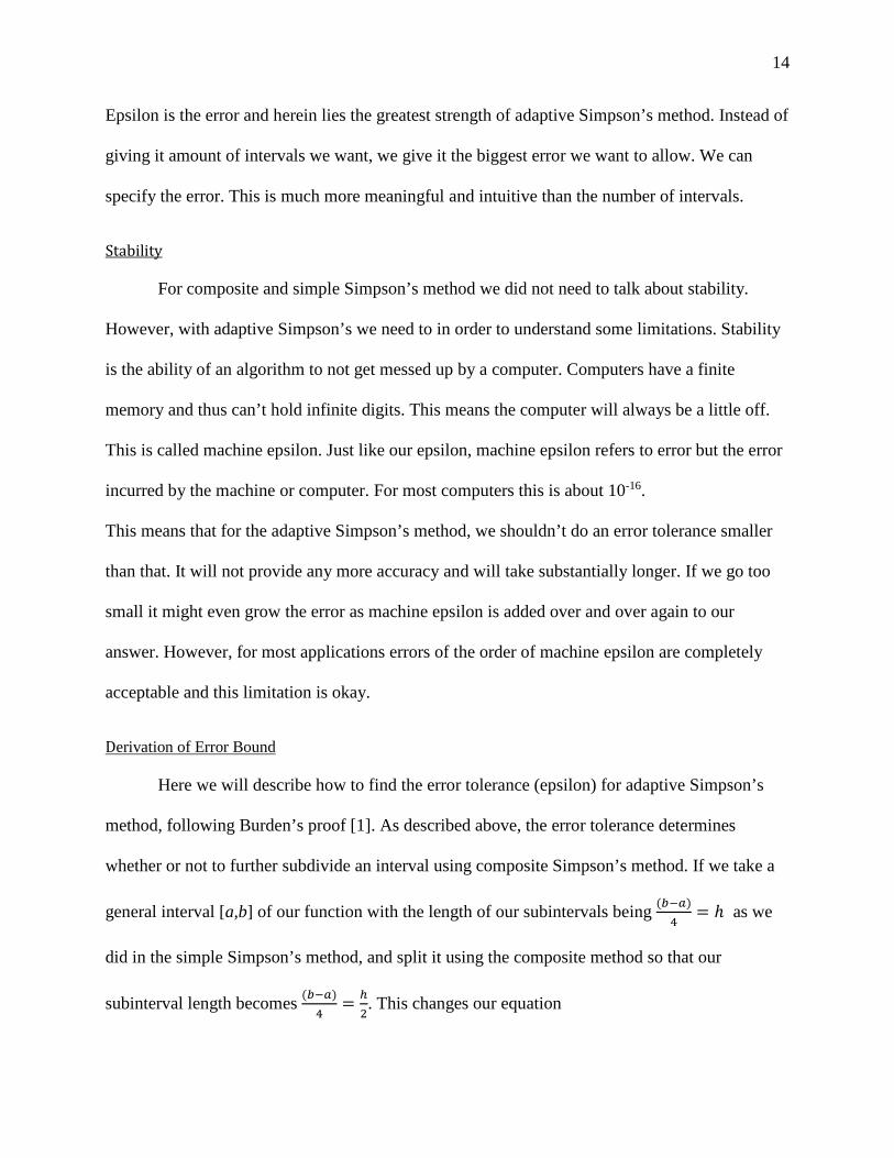
Formulaic Representation. Adaptive

Simpson’s method has no formula of its own. Instead it uses the formulas for simple and

composite Simpson’s method and compares the answer according to this formula below:

Figure 5: Adaptive Simpson's

(14)

14

Epsilon is the error and herein lies the greatest strength of adaptive Simpson’s method. Instead of

giving it amount of intervals we want, we give it the biggest error we want to allow. We can

specify the error. This is much more meaningful and intuitive than the number of intervals.

Stability

For composite and simple Simpson’s method we did not need to talk about stability.

However, with adaptive Simpson’s we need to in order to understand some limitations. Stability

is the ability of an algorithm to not get messed up by a computer. Computers have a finite

memory and thus can’t hold infinite digits. This means the computer will always be a little off.

This is called machine epsilon. Just like our epsilon, machine epsilon refers to error but the error

incurred by the machine or computer. For most computers this is about 10-16.

This means that for the adaptive Simpson’s method, we shouldn’t do an error tolerance smaller

than that. It will not provide any more accuracy and will take substantially longer. If we go too

small it might even grow the error as machine epsilon is added over and over again to our

answer. However, for most applications errors of the order of machine epsilon are completely

acceptable and this limitation is okay.

Derivation of Error Bound

Here we will describe how to find the error tolerance (epsilon) for adaptive Simpson’s

method, following Burden’s proof [1]. As described above, the error tolerance determines

whether or not to further subdivide an interval using composite Simpson’s method. If we take a

general interval [a,b] of our function with the length of our subintervals being (𝑏𝑏−𝑎𝑎)4

= ℎ as we

did in the simple Simpson’s method, and split it using the composite method so that our

subinterval length becomes (𝑏𝑏−𝑎𝑎)4

= ℎ2. This changes our equation

15

to

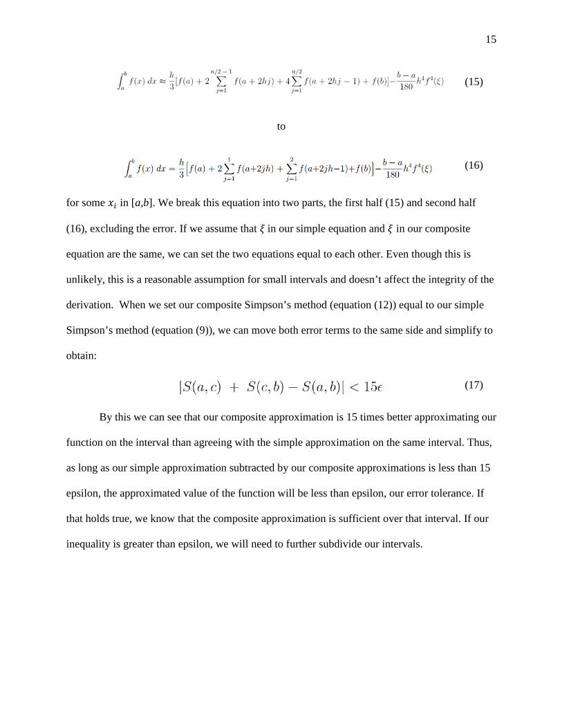
for some 𝑥𝑥𝑖𝑖 in [a,b]. We break this equation into two parts, the first half (15) and second half

(16), excluding the error. If we assume that 𝜉𝜉 in our simple equation and 𝜉𝜉 in our composite

equation are the same, we can set the two equations equal to each other. Even though this is

unlikely, this is a reasonable assumption for small intervals and doesn’t affect the integrity of the

derivation. When we set our composite Simpson’s method (equation (12)) equal to our simple

Simpson’s method (equation (9)), we can move both error terms to the same side and simplify to

obtain:

By this we can see that our composite approximation is 15 times better approximating our

function on the interval than agreeing with the simple approximation on the same interval. Thus,

as long as our simple approximation subtracted by our composite approximations is less than 15

epsilon, the approximated value of the function will be less than epsilon, our error tolerance. If

that holds true, we know that the composite approximation is sufficient over that interval. If our

inequality is greater than epsilon, we will need to further subdivide our intervals.

(15)

(16)

(17)

16

Appraisal

Table 3: Adaptive Simpson's

The adaptive Simpson’s method has various advantages and disadvantages. The greatest

advantage of it is the ability the user has to specify a certain error tolerance for the method to

consider, as explained in the previous section. It will then give an approximation that is

guaranteed to be accurate within the given error tolerance. As a result, this process can be as

accurate as the user desires. The main disadvantage is that the process is far more complicated

than the previous two methods. This method requires the computer to make decisions whether

certain intervals lie within the given error tolerance, and then to constantly repeat the process for

the smaller intervals that did not lie within the tolerance. This makes the code far more difficult

and time-consuming to write. It also increases the time the computer will take to calculate the

approximation, especially for very small error tolerances. This method is only considered to be

effective if a specific amount of accuracy is desired. Otherwise, the composite Simpson’s rule is

an accurate and far less complex method.

VI. TWO-THIRDS SIMPSON’S METHOD

Strategy of Method

The Simpson’s methods so far have an undesirable trait associated with them. They give

points different weights. This gives an asymmetrical feel to formula and makes us ask why they

17

have different weights. If we look at the derivation of the simple Simpson’s method, we can see

that we are most interested what the function is doing in the middle of the interval than on the

edges so that point gets more weight. However, the adaptation we use with the composite

Simpson’s method seems to give different middle points different weights. Thus also the

adaptive Simpson’s method which uses composite Simpson’s rule is also unsymmetrical.

We would not only love to find a Simpson’s rule variant that give equal weights to the middle

points but also a variant that is better. According to Dr. Daniel Velleman in his paper “Simpson

Symmetrized and Surpassed” the two-thirds Simpson’s method does the job [6].

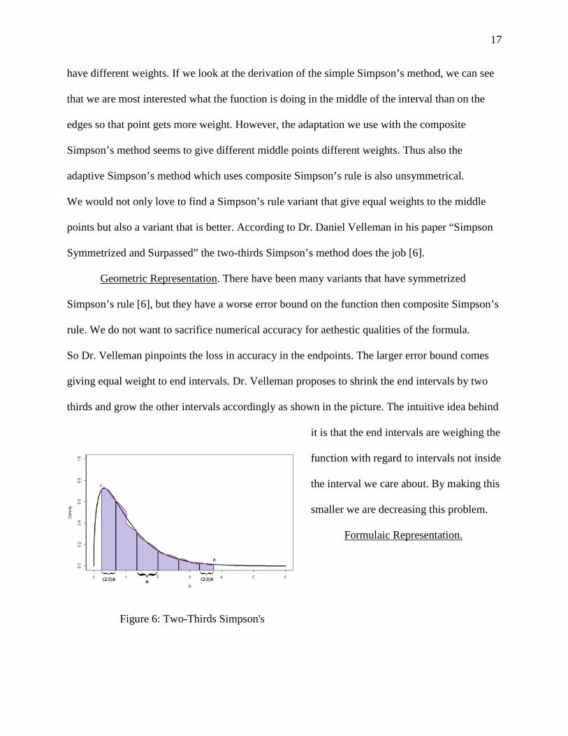
Geometric Representation. There have been many variants that have symmetrized

Simpson’s rule [6], but they have a worse error bound on the function then composite Simpson’s

rule. We do not want to sacrifice numerical accuracy for aethestic qualities of the formula.

So Dr. Velleman pinpoints the loss in accuracy in the endpoints. The larger error bound comes

giving equal weight to end intervals. Dr. Velleman proposes to shrink the end intervals by two

thirds and grow the other intervals accordingly as shown in the picture. The intuitive idea behind

it is that the end intervals are weighing the

function with regard to intervals not inside

the interval we care about. By making this

smaller we are decreasing this problem.

Formulaic Representation.

Figure 6: Two-Thirds Simpson's

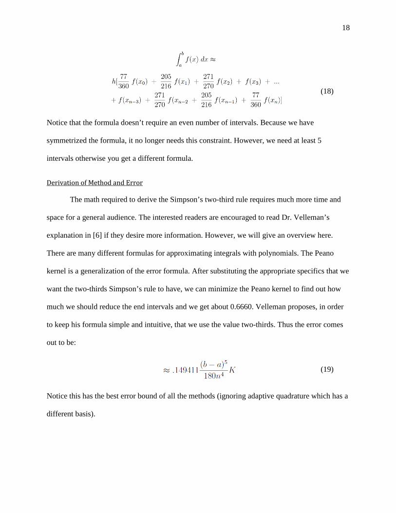
18

Notice that the formula doesn’t require an even number of intervals. Because we have

symmetrized the formula, it no longer needs this constraint. However, we need at least 5

intervals otherwise you get a different formula.

Derivation of Method and Error

The math required to derive the Simpson’s two-third rule requires much more time and

space for a general audience. The interested readers are encouraged to read Dr. Velleman’s

explanation in [6] if they desire more information. However, we will give an overview here.

There are many different formulas for approximating integrals with polynomials. The Peano

kernel is a generalization of the error formula. After substituting the appropriate specifics that we

want the two-thirds Simpson’s rule to have, we can minimize the Peano kernel to find out how

much we should reduce the end intervals and we get about 0.6660. Velleman proposes, in order

to keep his formula simple and intuitive, that we use the value two-thirds. Thus the error comes

out to be:

Notice this has the best error bound of all the methods (ignoring adaptive quadrature which has a

different basis).

(18)

(19)

19

Appraisal

Table 4: Two-Thirds Simpson's

Sadly for our problem the two-thirds Simpson’s method does not perform as well. It

seems that for small numbers of intervals, the two-thirds Simpson’s method does not do well.

The reason for this is that for the gamma distribution, the end intervals are very important,

especially on the right side. Two-thirds Simpson’s method puts most of the weight in the middle

of the interval. For most functions, that’s all you have to worry about but for the gamma

distribution the ends of the intervals are very important. This does not fare well in terms of error

with any but the simple Simpson’s method.

20

VII. COMPARISON

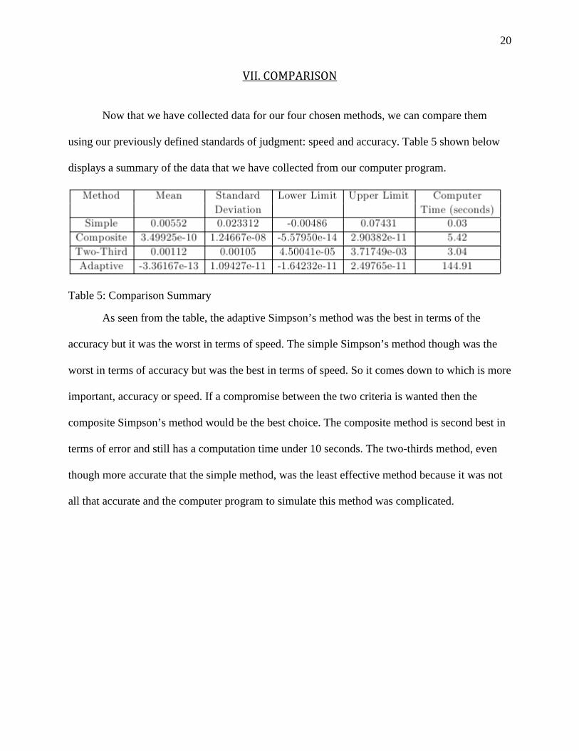
Now that we have collected data for our four chosen methods, we can compare them

using our previously defined standards of judgment: speed and accuracy. Table 5 shown below

displays a summary of the data that we have collected from our computer program.

Table 5: Comparison Summary

As seen from the table, the adaptive Simpson’s method was the best in terms of the

accuracy but it was the worst in terms of speed. The simple Simpson’s method though was the

worst in terms of accuracy but was the best in terms of speed. So it comes down to which is more

important, accuracy or speed. If a compromise between the two criteria is wanted then the

composite Simpson’s method would be the best choice. The composite method is second best in

terms of error and still has a computation time under 10 seconds. The two-thirds method, even

though more accurate that the simple method, was the least effective method because it was not

all that accurate and the computer program to simulate this method was complicated.

21

VIII. CONCLUSION

Through our findings, we have discovered that the least effective approximation method

for the gamma distribution is the two-thirds Simpson’s method. Not only was it not nearly as

accurate as the composite or adaptive Simpson’s methods, it involved much more complicated

coding then the simple or composite methods and took the computer a significant amount of time

to compute. The other approximation methods have a varying degree of effectiveness. The

adaptive Simpson’s method is the most accurate approximation given the fact that it will give an

estimate within a certain error bound specified by the user. However, this method took the

computer the longest time to compute, by far. The simple Simpson’s rule is the least accurate

method but easily had the simplest coding involved. That is evident by the fact that it only took

the computer 0.03 seconds to compute the answer. Taking this all into account, we found that the

most effective approximation method was the composite method. It was the second most

accurate test and took the computer only a slightly longer time to compute than the two-thirds

method. Of course, if less subintervals are used, the calculation times becomes faster while the

accuracy decreases. As such, this method provides a very accurate approximation and a

relatively fast computation speed with the option of using less subintervals for those who desire

the calculation in even less time.

Since the scope of this paper did not allow for exploration of all the different methods of

numerical quadrature analysis, the curious reader can research additional methods, such as

Simpson’s three-eighths rule, Simpson’s one-third rule, and the generalized Simpson’s rule [7].

Changing the scale and size of our gamma function will also yield different and interesting

results. Another avenue to consider is applying and combining existing methods. Perhaps by

applying the adaptive method to our two-thirds method, we would be able to obtain even more

22

accuracy. These Simpson’s methods could also be compared to other quadrature methods like

Gaussian quadrature which doesn’t use the midpoint of intervals. These derivations are left for

the reader to pursue.

23

REFERENCES

[1] Burden, Richard L. Faires, J. Douglas. Numerical Analysis Ninth Edition. Brooks/Cole

Cengage Learning, 2011.

[2] Davis, P. J., & Rabinowitz, P. (1984). Methods of numerical integration. (2nd ed., Vol. 1).

Orlando: Academic Press, INC.

[3] Stewart J. (2012). Single Variable Calculus: Early Transcendentals 7th ed. Vol. 2. Belmont,

CA. Brooks/Cole, Cengage Learning.

[4] Schroder, J. (2006). Lecture 24: Simpson’s Rule [PowerPoint slides]. Retrieved from

http://lukeo.cs.illinois.edu/static_courses/2006spring/CS257/lectures/lecture24.pdf

[5] Schervish, M. J., & DeGroot, M.H. (2010). Probability and Statistics. (4th ed.). Boston.

Addison-Wesley.

[6] Velleman, Daniel J. (2004). “Simpson Symmetrized and Surpassed”. Mathematical

Association of America. Mathematics Magazine. Volume 77, Number 1, p. 31-45.

[7] Velleman, Daniel J. (2005). “The Generalized Simpson’s Rule”. The American Mathematical

Monthly. Volume 112, No. 4, p. 342-350.

[8] Zwillinger, D. (1992). Handbook of Integration. United States of America. Jones and Bartlett

Publishers, Inc.

24

APPENDIXES

Appendix A: Related theorems

Weighted Mean Value Theorem for Integrals: Suppose f is a continuous function on the interval

[a,b], the Riemann integral of g exists on [a,b], and g(x) does not change sign on [a,b].

Then there exists a number c in (a,b) with ∫ 𝑓𝑓(𝑥𝑥)𝑔𝑔(𝑥𝑥)𝑑𝑑𝑥𝑥 = 𝑓𝑓(𝑐𝑐)∫ 𝑔𝑔(𝑥𝑥)𝑑𝑑𝑥𝑥𝑏𝑏𝑎𝑎

𝑏𝑏𝑎𝑎

Intermediate Value Theorem: If f is a continuous function on the interval [a,b], and K is any

number between f(a) and f(b), then there exists a number c in (a,b) for which f(c)=K.

Second Derivative Midpoint Formula:

𝑓𝑓"(𝑥𝑥0) = 1ℎ2

[𝑓𝑓(𝑥𝑥0 − ℎ) − 2𝑓𝑓(𝑥𝑥0) + 𝑓𝑓(𝑥𝑥0 + ℎ)] − ℎ2

12𝑓𝑓(4)(𝜉𝜉)

For some 𝜉𝜉, where 𝑥𝑥0 − ℎ < 𝜉𝜉 < 𝑥𝑥0 + ℎ.

25

Appendix B: Original Code

#316 code x<-seq(0,6,length=1000) plot(x,dgamma(x,1.5, rate=1.5), type='l', ylim=c(0,1), main="Gamma Distribution", xlab="X", ylab="Density" ) #dgamma is the function that we are plotting abline(v=4.6) abline(v=5.6) #v is for vertical line #h is for horizontal line #Simple Simpson's function for the gamma distribution gammasimple<-function(a, b){ h<-(b-a)/2 out<- (h/3)*(dgamma(a,1.5,rate=1.5)+4*dgamma(a+h,1.5,rate=1.5)+dgamma(b,1.5,rate=1.5)) return(out) } #Composite Simpson's function for the gamma distribution gammacomp<-function(a,b,n){ h<-(b-a)/n suma=0 sumb=0 totala = n/2-1 if(totala>0){ for(i in 1:totala){ suma= suma+dgamma(a+2*h*i,1.5,rate=1.5)} } for(i in 1:(n/2)){ sumb= sumb+dgamma(a+h*(2*i-1),1.5,rate=1.5) } out<- (h/3)*(dgamma(a,1.5,rate=1.5)+dgamma(b,1.5,rate=1.5)+2*suma+4*sumb) return(out) } #2/3 Simpson's method for the gamma distribution

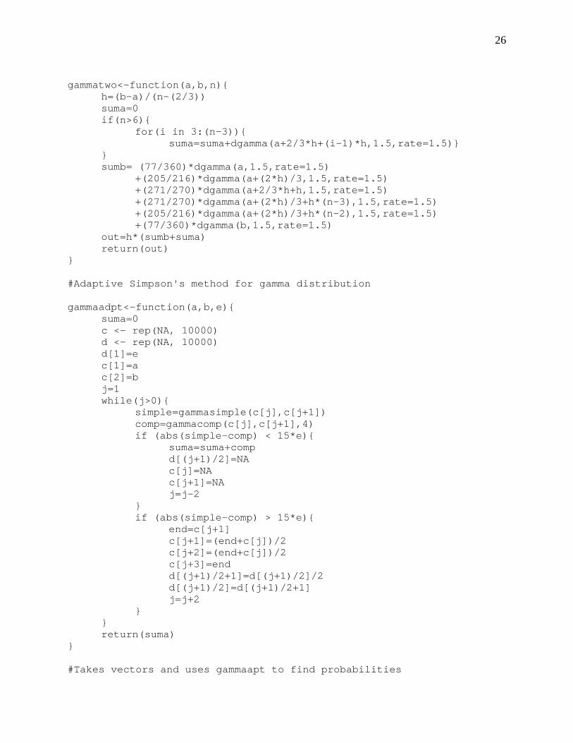
26

gammatwo<-function(a,b,n){ h=(b-a)/(n-(2/3)) suma=0 if(n>6){ for(i in 3:(n-3)){ suma=suma+dgamma(a+2/3*h+(i-1)*h,1.5,rate=1.5)} } sumb= (77/360)*dgamma(a,1.5,rate=1.5) +(205/216)*dgamma(a+(2*h)/3,1.5,rate=1.5) +(271/270)*dgamma(a+2/3*h+h,1.5,rate=1.5) +(271/270)*dgamma(a+(2*h)/3+h*(n-3),1.5,rate=1.5) +(205/216)*dgamma(a+(2*h)/3+h*(n-2),1.5,rate=1.5) +(77/360)*dgamma(b,1.5,rate=1.5) out=h*(sumb+suma) return(out) } #Adaptive Simpson's method for gamma distribution gammaadpt<-function(a,b,e){ suma=0 c <- rep(NA, 10000) d <- rep(NA, 10000) d[1]=e c[1]=a c[2]=b j=1 while(j>0){ simple=gammasimple(c[j],c[j+1]) comp=gammacomp(c[j],c[j+1],4) if (abs(simple-comp) < 15*e){ suma=suma+comp d[(j+1)/2]=NA c[j]=NA c[j+1]=NA j=j-2 } if (abs(simple-comp) > 15*e){ end=c[j+1] c[j+1]=(end+c[j])/2 c[j+2]=(end+c[j])/2 c[j+3]=end d[(j+1)/2+1]=d[(j+1)/2]/2 d[(j+1)/2]=d[(j+1)/2+1] j=j+2 } } return(suma) } #Takes vectors and uses gammaapt to find probabilities

27

vadpt = function(x,y,e){ out = rep(NA, length(x)) if(length(x)==length(y)){ for (i in 1:length(x)){ out[i]=gammaadpt(x[i],y[i],e) } } return(out) } #Random tests #Generate the random intervals to test on x = runif(5000,min=0,max=3) z = runif(5000,min=0,max=3) y= x+z #Find the approximations and compute the time taken to do so intervals = c(6,8,10,100,1000) error = c(1,10^-2,10^-6,10^-12) simpletime = system.time({ simpleans = t(gammasimple(x,y)) }) comptime = rep(0,length(intervals)) compans = matrix(NA,length(x),length(intervals)) for (i in 1:length(intervals)){ comptime[i] = system.time({ compans[,i] = t(gammacomp(x,y,intervals[i])) })[3] } twotime = rep(0,length(intervals)) twoans = matrix(NA,length(x),length(intervals)) for (i in 1:length(intervals)){ twotime[i] = system.time({ twoans[,i] = t(gammatwo(x,y,intervals[i])) })[3] } adpttime = rep(0,length(error)) adptans = matrix(NA,length(x),length(error)) for (i in 1:length(error)){ print(i) adpttime[i] = system.time({ adptans[,i] = t(vadpt(x,y,error[i])) })[3] }

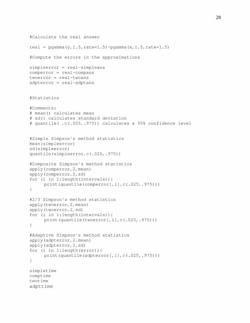
28

#Calculate the real answer real = pgamma(y,1.5,rate=1.5)-pgamma(x,1.5,rate=1.5) #Compute the errors in the approximations simpleerror = real-simpleans comperror = real-compans twoerror = real-twoans adpterror = real-adptans #Statistics #Comments: # mean() calculates mean # sd() calculates standard deviation # quantile( ,c(.025,.975)) calculates a 95% confidence level #Simple Simpson's method statistics mean(simpleerror) sd(simpleerror) quantile(simpleerror,c(.025,.975)) #Composite Simpson's method statistics apply(comperror,2,mean) apply(comperror,2,sd) for (i in 1:length(intervals)){ print(quantile(comperror[,i],c(.025,.975))) } #2/3 Simpson's method statistics apply(twoerror,2,mean) apply(twoerror,2,sd) for (i in 1:length(intervals)){ print(quantile(twoerror[,i],c(.025,.975))) } #Adaptive Simpson's method statistics apply(adpterror,2,mean) apply(adpterror,2,sd) for (i in 1:length(error)){ print(quantile(adpterror[,i],c(.025,.975))) } simpletime comptime twotime adpttime

29

Appendix C: Assignment Foundation

Purpose: The purpose of this assignment is to conduct our own original experiment and to report

on our findings. This project is the main focus of this class; therefore, there are many sub-

purposes of this assignment. Through this project we will learn how to effectively communicate

research as well as how to conduct our own research. Our chosen research topic is integral

approximation. In this report we propose to explore different methods, all variations of

Simpson’s method, in approximating the gamma distribution. Our research and experimentation

must be presented clearly and accurately, not necessarily to persuade the reader to a specific

action, but to inform them, and perhaps to peak their interest in the field of mathematics

involving approximating integrals. We hope to clearly communicate our findings by means of

graphs, tables, and formulas, with explanations of each.

Audience: The audience for this assignment is our instructor and fellow classmates. Therefore,

when writing our report we should keep in mind that not everyone reading this report will be

experts in our topic. We have assumed a basic understanding of calculus and mathematics in

general. Our audience is educated and intelligent, and should not be patronized. This report is

designed to make the reader think, and the reader should not feel spoon-fed. Most people do not

have much of an interest in calculus, so our report should be interesting and engaging. Our

instructor Liz is looking not so much at the correctness and rigor of our research, but rather the

correctness and rigor of our writing. She is looking for a paper that has cut down the lard, that

clearly illustrates a point, that is concise and consistent, and that is able to communicate the ideas

in the paper.

Scope: This project should be at least 15 pages in length without any added graphics but no more

than 20 pages at Liz’s request. This allows us to elaborate on our four chosen methods, but not to

30

explore many more than that. We researched and experimented with simple, composite, adaptive,

and two-thirds Simpson’s methods. We have included much information on these methods,

including derivations of the formulae for the approximation itself as well as the error. Also

included is our experimentation, as we took multiple approximations of the same integral with

the different methods to compare them. Since the majority of our paper is based on original

research, we have less cited sources than may be expected. We do have included in our appendix

much of our original code. We drew on the research of others for derivations and assumptions

that could not be explained in the allotted page limit, but the majority of our equations were

worked out by ourselves.

Format: This project is to be submitted as a hard copy and is to be spiral bound. There is a

formatting guide that has been placed on learning suite and we are to follow that format exactly

when writing this report. We have prefatory elements, which include a title page, table of

contents, lists of figures and tables, and an abstract; as well as the bulk of our report, which is

organized with headings, subheadings, and sub-subheadings. Following the body of our report is

our appendix, which is where our assignment foundation will be included, as well as other

relevant information.

Schedule: This project has a lot of subprojects that are due that will help us finish this technical

report. These include the Journal Article Analysis White Paper, Proposal, Conflict Resolution

Memo, and Critique. The final draft of our technical report is due April 9, 2014. There is no

rough draft due for this project; therefore, our group needs to stay on top of our decided schedule

in our proposal. As a group we meet at least weekly on Saturday mornings to work together on

our project.

31

Appendix D: Sample of Formatting