Report on FY15 Alloy 617 Code Rules Development

ORNL/TM-2015/487

Report on FY15 Alloy 617 Code Rules Development

T.-L. Sham R.I. Jetter

G. Hollinger D. Pease P. Carter

C. Pu Y. Wang

September 9, 2015

Approved for public release; distribution is unlimited.

DOCUMENT AVAILABILITY

Reports produced after January 1, 1996, are generally available free via US Department of Energy (DOE) SciTech Connect. Website http://www.osti.gov/scitech/ Reports produced before January 1, 1996, may be purchased by members of the public from the following source: National Technical Information Service 5285 Port Royal Road Springfield, VA 22161 Telephone 703-605-6000 (1-800-553-6847) TDD 703-487-4639 Fax 703-605-6900 E-mail [email protected] Website http://www.ntis.gov/help/ordermethods.aspx

Reports are available to DOE employees, DOE contractors, Energy Technology Data Exchange representatives, and International Nuclear Information System representatives from the following source: Office of Scientific and Technical Information PO Box 62 Oak Ridge, TN 37831 Telephone 865-576-8401 Fax 865-576-5728 E-mail [email protected] Website http://www.osti.gov/contact.html

This report was prepared as an account of work sponsored by an agency of the United States Government. Neither the United States Government nor any agency thereof, nor any of their employees, makes any warranty, express or implied, or assumes any legal liability or responsibility for the accuracy, completeness, or usefulness of any information, apparatus, product, or process disclosed, or represents that its use would not infringe privately owned rights. Reference herein to any specific commercial product, process, or service by trade name, trademark, manufacturer, or otherwise, does not necessarily constitute or imply its endorsement, recommendation, or favoring by the United States Government or any agency thereof. The views and opinions of authors expressed herein do not necessarily state or reflect those of the United States Government or any agency thereof.

http://www.osti.gov/scitech/

http://www.ntis.gov/help/ordermethods.aspx

http://www.osti.gov/contact.html

ORNL/TM-2015/487

Advanced Reactor Technologies Program

Report on FY15 Alloy 617 Code Rules Development

T.-L. Sham, R.I. Jetter

1, G. Hollinger

2, D. Pease

2, P. Carter

3, C. Pu

4, and Y. Wang

1 Consultant

2 Becht Engineering Co., Inc.

3 Stress Engineering Services, Inc.

4 University of Tennessee

Date Published: September 9, 2015

Prepared under the direction of the

U.S. Department of Energy

Office of Nuclear Energy

Prepared by

OAK RIDGE NATIONAL LABORATORY

Oak Ridge, TN 37831-6283

managed by

UT-BATTELLE, LLC

for the

US DEPARTMENT OF ENERGY

under contract DE-AC05-00OR22725

iv

Intentionally Blank

v

CONTENTS

Content ................................................................................................................................................... Page

CONTENTS .................................................................................................................................................. v LIST OF FIGURES FOR PART I .............................................................................................................. vii LIST OF FIGURES FOR PART II .............................................................................................................. ix LIST OF TABLES FOR PART I ................................................................................................................. xi LIST OF TABLES FOR PART II ............................................................................................................... xi ACKNOWLEDGMENTS ......................................................................................................................... xiii ABSTRACT .................................................................................................................................................. 1 INTRODUCTION ........................................................................................................................................ 3 PART I – BACKGROUND FOR EPP STRAIN LIMITS CODE CASE..................................................... 4

I-1. THEORETICAL BASIS ............................................................................................................... 4 I-1.1 Development of Bounding Concepts ................................................................................ 4 I-1.2 Limiting Solutions ............................................................................................................. 5 I-1.3 Energy and Work Bounds ................................................................................................. 5

I-2 OUTLINE OF EPP STRAIN LIMITS CODE CASE .................................................................... 7 I-3 EXAMPLE PROBLEMS ............................................................................................................... 9

I-3.1 Representative Example Problem ..................................................................................... 9 I-3.2 Strain Limits Code Case to Subsection HB, Subpart B Comparison .............................. 19

I-4 EXPERIMENTAL RESULTS COMPARISON .......................................................................... 26 I-4.1 Two-Bar Test Evaluation ................................................................................................ 26

I-5 ANALYTICAL COMPARISONS ............................................................................................... 30 I-5.1 Background ..................................................................................................................... 30 I-5.2 Bounding Theories .......................................................................................................... 30 I-5.3 Material Properties and Pseudo Yield Stress................................................................... 31 I-5.4 Inelastic Strain Limits and Ratcheting Analyses ............................................................. 32 I-5.5 Bounding Theory Example Calculations ........................................................................ 38

I-6 SUMMARY AND CONCLUSIONS ........................................................................................... 38 I-6.1 Basis Of The Code Case Methodology ........................................................................... 38 I-6.2 Representative Example Problem ................................................................................... 39 I-6.3 Strain Limits Code Case to Subsection HB, Subpart B Comparison .............................. 39 I-6.4 Experimental Comparison ............................................................................................... 40 I-6.5 Analytical Comparison .................................................................................................... 40 I-6.6 Conclusions ..................................................................................................................... 41

I-APPENDIX A: RATCHETING ANALYSIS .......................................................................................... 42 I-APPENDIX B: DRAFT EPP STRAIN LIMITS CODE CASE ............................................................... 44 PART II – BACKGROUND FOR EPP CREEP-FATIGUE CODE CASE ............................................... 49

II-1 THEORETICAL BASIS ............................................................................................................. 49 II-1.1 Shakedown Analysis for Cyclic Creep Damage ............................................................ 49

II-2. OUTLINE OF EPP CREEP-FATIGUE CODE CASE ............................................................. 51 II-3. EXAMPLE PROBLEMS ........................................................................................................... 52

II-3.1 Representative Example Problem .................................................................................. 52 II-3.2 Creep-Fatigue Code Case to Subsection HB, Subpart B Comparison ........................... 63

II-4. BOUNDING THEORY EXAMPLE CALCULATION ............................................................ 69 II-4.1 Analysis of Strain Controlled Creep-Fatigue Test Specimen ........................................ 69 II-4.2 Process Flow Procedure for Bounding Creep Damage in Creep-Fatigue Specimen ..... 71

II-5 EXPERIMENTAL RESULTS COMPARISON ........................................................................ 74

vi

II-5.1 Experimental Procedure ................................................................................................. 74 II-5.2 Elastic-Perfectly Plastic Simulation on Alloy 617 Creep-Fatigue ................................. 76 II-5.3 Standard Alloy 617 Creep-Fatigue Tests ....................................................................... 77 II-5.4 Alloy 617 SMT Test Articles ......................................................................................... 79 II-5.5 316H Stainless Steel SMT Test ..................................................................................... 86 II-5.6 Comparison Based on Allowable Design Life ............................................................... 88

II-6 SUMMARY AND CONCLUSIONS ......................................................................................... 90 II-6.1 Background .................................................................................................................... 90 II-6.2. Theoretical Basis ............................................................................................................ 90 II-6.3 Example Problems ......................................................................................................... 91 II-6.4 Bounding Theory Example Calculations ....................................................................... 92 II-6.5 Experimental Results ..................................................................................................... 92 II-6.6 Conclusions .................................................................................................................... 92

II-APPENDIX A ......................................................................................................................................... 93 II-APPENDIX B: DRAFT EPP CREEP-FATIGUE CODE CASE ........................................................... 97 REFERENCES ......................................................................................................................................... 102

vii

LIST OF FIGURES FOR PART I

Figure ................................................................................................................................................... Page

Fig. I-1. Representative Example Problem Configuration (dimensions in inches) .................................... 10 Fig. I-2. Service Level A Loads and Load Combinations; loadings versus time ....................................... 11 Fig. I-3. Service Level B Loads and Load Combinations; loadings versus time ....................................... 11 Fig. I-4. Service Level C Loads and Load Combinations; loadings versus time ....................................... 12 Fig. I-5. Level A and B Composite Cycle .................................................................................................. 13 Fig. I-6. Level A and C Composite Cycle .................................................................................................. 13 Fig. I-7. Nozzle to Sphere Example Problem FEA Mesh Without Weld Zone ......................................... 14 Fig. I-8. Nozzle to Sphere Example Problem FEA Mesh With Weld Zone .............................................. 15 Fig. I- 9. Level B Peak Up (1175

oF) ......................................................................................................... 16

Fig. I-10. Level A&B Composite Cycle Steps ........................................................................................... 17 Fig. I-11. Level A & C Composite Cycle Steps ......................................................................................... 17 Fig. I-12. Case 3 Component Pipe Geometry and Steady State Temperature (

oF) Contours ..................... 21

Fig. I-13. 316H SS Isochronous 1% Inelastic Strain Data ......................................................................... 22 Fig. I-14. Non Ratcheting Strain Histories for Tube 2 with Design and Thermal Stress x 1.0. Cyclic

strain (x) = 0.095. y = Core strain (y) = 0.0001. 1% Limit Demonstrated. ............................. 22 Fig. I-15. Contour Plot of Radial Deflection Differences Between Cycles. Design Pressure and

Thermal Loading x 1. Apparent Differences not Numerically Significant. Ratcheting

not Indicated. ........................................................................................................................... 23 Fig. I-16. Ratcheting Strain Histories for Tube 2 Intersection with Design and Thermal Stress x

1.2. Strain Limits Not Met. ...................................................................................................... 23 Fig. I-17. Contour Plot of Radial Deflection Differences Between Cycles. Design Pressure and

Thermal Stress x 1.2. Ratcheting in Intersection Indicates Strain Limits are Not Met. ......... 24 Fig. I-18. Non-Ratcheting Strain Histories for Tube 1 and Tube 2 Respectively. From the

Component Model. Design and Thermal Stress x 1.2. Cyclic Strain (x) = 0.096, y =

Core Strain (y) < 0.0002. 1% Limit Demonstrated. ................................................................ 25 Fig. I-19. Schematic of Two-bar thermal ratcheting condition (a) and the equivalent boundary

conditions of the two bars (b) .................................................................................................. 26 Fig. I-20. Temperature vs. time histogram for two-bar thermal ratcheting experiments on Alloy 617 ..... 27 Fig. I-21. The maximum and the minimum total strains in the two bars at temperature range 800ºC

to 950ºC (heating and cooling rates were 5 oC/min). .............................................................. 27

Fig. I-22. Two bar test data with 1% design envelope predictions from the strain limits code case

and inelastic analysis ............................................................................................................... 28 Fig. I-23. Alloy 617 Inelastic Stress – Strain Rates and Material Model Parameters (Units:

oF,

hours, ksi, BTU, lbs) ............................................................................................................... 31 Fig. I-24. Alloy 617 Stress versus Temperature for Yield and 1% Inelastic Strain in 200 Hours ............. 32 Fig. I-25. Through Wall Temperature Contours and Second Order Mesh ................................................ 33 Fig. I-26. Examples of Non-Ratcheting (a) and Ratcheting (b) Strain Histories ....................................... 33 Fig. I-27. EPP Ratcheting Analyses with Zero and Non-Zero Minimum Plastic Strain (y) ...................... 34 Fig. I-28. Tube Radial Nodal Displacements for Tube Case #3 Negative Pressure Loading .................... 35 Fig. I-29. Summary of EPP and Creep Analysis Load Cases on Bree Plot of Normalized Primary

and Thermal Stress .................................................................................................................. 36 Fig. I-30. OD and Bore Temperature Histories: 1 Hour Hold and 10 Minute Delay Between

Downshocks ............................................................................................................................ 37

viii

Intentionally Blank

ix

LIST OF FIGURES FOR PART II

Figure ................................................................................................................................................... Page

Fig. II-1. Representative Example Problem Configuration (dimensions are in inches)............................. 53 Fig. II-2. Service Level A Loads and Load Combinations; loadings versus time ..................................... 54 Fig. II-3. Service Level B Loads and Load Combinations; loadings versus time ...................................... 55 Fig. II-4. Service Level C Loads and Load Combinations; loadings versus time ...................................... 55 Fig. II-5. Level A and B Composite Cycle ................................................................................................ 56 Fig. II-6. Level A and C Composite Cycle ................................................................................................ 57 Fig. II-7. Nozzle to Sphere Example Problem FEA Mesh Without Weld Zone ........................................ 58 Fig. II-8. Nozzle to Sphere Example Problem FEA Mesh Without Weld Zone ........................................ 58 Fig. II-9. Level B Peak Up (1175

oF) ......................................................................................................... 59

Fig. II-10. Level A&B Composite Cycle Steps ......................................................................................... 60 Fig. II-11. Level A & C Composite Cycle Steps ....................................................................................... 60 Fig. II-12. Hoop Pressure Plus Thermal Stress. Maximum Value of both Stresses is 44 ksi.

Second Order Finite Element Mesh Indicated. .............................................................................. 64 Fig. II-13. 316H Stainless Isochronous Creep Rupture Stress – Temperature Curves .............................. 67 Fig. II-14. Contours of Analysis Plastic Strain. Maximum value in the Bore of Tube #2 ........................ 67 Fig. II-15. Plots of Cyclic Plastic Strain from Tube Bore. Shakedown Obtained for 10,000 Hours

Rupture Life, Failure to Shakedown for 12,000 Hours Rupture Life ............................................ 68 Fig. II-16. Stress and damage histories for 1 hour cycle time .................................................................... 70 Fig. II-17. Stress and damage histories for 10 hour cycle time .................................................................. 71 Fig. II-18. Effect of Cycle Time on EPP Conservatism ............................................................................. 71 Fig. II-19. Applied Loading ....................................................................................................................... 72 Fig. II-20. EPP Solution ............................................................................................................................. 72 Fig. II-21. EPP Solution with Period t ....................................................................................................... 73 Fig. II-22. Bounding solution Compared to Analytical Solution ............................................................... 73 Fig. II-23. SMT methodology .................................................................................................................... 74 Fig. II-24. Type 1 SMT specimen geometry. ............................................................................................. 75 Fig. II-25. Strain range history of Alloy 617 Type 1 SMT ........................................................................ 75 Fig. II-26. Stress relaxation during the hold period for Type 1 SMT necked test section and

standard creep-fatigue specimen, Carroll et al. (2010). ................................................................. 76 Fig. II-27. Drawings for the Two SMT Test Articles (Dimensions in Inches) .......................................... 80 Fig. II-28. Test setup of the SMT specimen. ............................................................................................. 81 Fig. II-29. Profiles of L for imposing the prescribed displacements over the gage length L for

Alloy 617. Displacement hold was applied at the maximum tensile L value. Cycles

were fully reversed. ........................................................................................................................ 82 Fig. II-30. Typical axisymmetric finite element meshes for Type I and Type II SMT test articles ........... 83 Fig. II-31. Plots of ABAQUS active plasticity variable AC YIELD for Alloy 167. Essentially

grey color indicates active plasticity and blue color denotes incremental elastic response. .......... 85 Fig. II-32. Profile of L for imposing the prescribed displacements over the gage length L for

316H............................................................................................................................................... 87 Fig. II-33. Contour plot of ABAQUS active plasticity variable AC YIELD for 316H. Essentially

grey color indicates active plasticity and blue color denotes incremental elastic response. .......... 87 Fig. II-34. Creep-fatigue code case allowable life comparison to Alloy 617 SMT data ........................... 89 Fig. II-35. Creep-fatigue code case allowable life comparison to 316H stainless steel SMT data ............ 89

x

Intentionally Blank

xi

LIST OF TABLES FOR PART I

Table ................................................................................................................................................... Page

Table I-1. Nature of work bounds for increasing different levels of problem complexity. ......................... 6 Table I-2. Thermo-Mechanical Properties of TP316H at 1100

oF ............................................................. 20

Table I-3. Summary of HBB-T-1332 Test B1 and B2 Strain Limits Calculations .................................... 20 Table I-4. Results of Ratcheting Calculations of Plain Tubes and Tapered Joined Tube .......................... 25 Table I-5. Two bar test data parameters ..................................................................................................... 29 Table I-6. Design Data ............................................................................................................................... 32 Table I-7. Results of Ratcheting Calculations for Alloy 617 ..................................................................... 34 Table I-8. Inelastic Displacements and Strains .......................................................................................... 35 Table I-9. Results of EPP Analyses ........................................................................................................... 37 Table I-10. Results of Creep Analyses ....................................................................................................... 37

LIST OF TABLES FOR PART II

Table ................................................................................................................................................... Page

Table II-1. Thermo-mechanical properties of TP316 at 1100 oF ............................................................... 64

Table II-2. Thermo-mechanical bore strain range: Tube 2 (HBB-T-1413) ............................................... 65 Table II-3. Tube 2 strain range per cycle ................................................................................................... 66 Table II-4. Hot relaxation and creep damage calculation: Tube 2 ............................................................. 66 Table II-5. Tube 2 creep-fatigue life calculation HBB-T-1411 ................................................................. 66 Table II-6. Tube 2 creep-fatigue life calculation EPP shakedown analysis ............................................... 68 Table II-7. Creep and damage constants for 316H stainless steel at 1400

oF. Units: ksi,

oF, hours ........... 69

Table II-8. Test conditions and data of Alloy 617 standard ASTM creep-fatigue test specimens ............ 78 Table II-9. Evaluation of the elastic shakedown condition for the standard Alloy 617 creep-

fatigue test specimen geometry ...................................................................................................... 79 Table II-10. SMT test conditions and data for Alloy 617 .......................................................................... 81 Table II-11. Material parameters used in the EPP finite element analyses for Alloy 617 ......................... 86 Table II-12. SMT test conditions and data for 316H SS ............................................................................ 86 Table II-13. Material parameters used in the EPP finite element analysis for 316H ................................. 88 Table II-14. Experimental data – Alloy 617 at 950

oC................................................................................ 88

Table II-15. Experimental data – 316H stainless steel at 815oC ................................................................ 89

xii

Intentionally Blank

xiii

ACKNOWLEDGMENTS

This research was sponsored by the U.S. Department of Energy (DOE), Office of Nuclear Energy

(NE), for the Advanced Reactor Technologies (ART) Program. We gratefully acknowledge the support

provided by Carl Sink of DOE-NE, ART Program Manager; William Corwin of DOE-NE, ART

Materials Technology Lead; David Petti of Idaho National Laboratory (INL), ART Co-National

Technical Director; and Richard Wright of INL, Technical Lead, High Temperature Materials. The time

spent by Hong Wang of ORNL in reviewing this report is greatly appreciated.

xiv

Intentionally Blank

1

ABSTRACT

Due to its strength at very high temperatures, up to 950°C (1742°F), Alloy 617 is the reference

construction material for structural components that operate at or near the outlet temperature of the very

high temperature gas-cooled reactors. However, the current rules in the ASME Section III, Division 5

Subsection HB, Subpart B for the evaluation of strain limits and creep-fatigue damage using simplified

methods based on elastic analysis have been deemed inappropriate for Alloy 617 at temperatures above

650°C (1200°F) (Corum and Brass, Proceedings of ASME 1991 Pressure Vessels and Piping Conference,

PVP-Vol. 215, p.147, ASME, NY, 1991). The rationale for this exclusion is that at higher temperatures it

is not feasible to decouple plasticity and creep, which is the basis for the current simplified rules. This

temperature, 650°C (1200°F), is well below the temperature range of interest for this material for the high

temperature gas-cooled reactors and the very high temperature gas-cooled reactors. The only current

alternative is, thus, a full inelastic analysis requiring sophisticated material models that have not yet been

formulated and verified.

To address these issues, proposed code rules have been developed which are based on the use of

elastic-perfectly plastic (EPP) analysis methods applicable to very high temperatures. The proposed rules

for strain limits and creep-fatigue evaluation were initially documented in the technical literature (Carter,

Jetter and Sham, Proceedings of ASME 2012 Pressure Vessels and Piping Conference, papers PVP 2012–

28082 and PVP 2012–28083, ASME, NY, 2012), and have been recently revised to incorporate

comments and simplify their application. Background documents have been developed for these two code

cases to support the ASME Code committee approval process. These background documents for the EPP

strain limits and creep-fatigue code cases are documented in this report.

2

Intentionally Blank

3

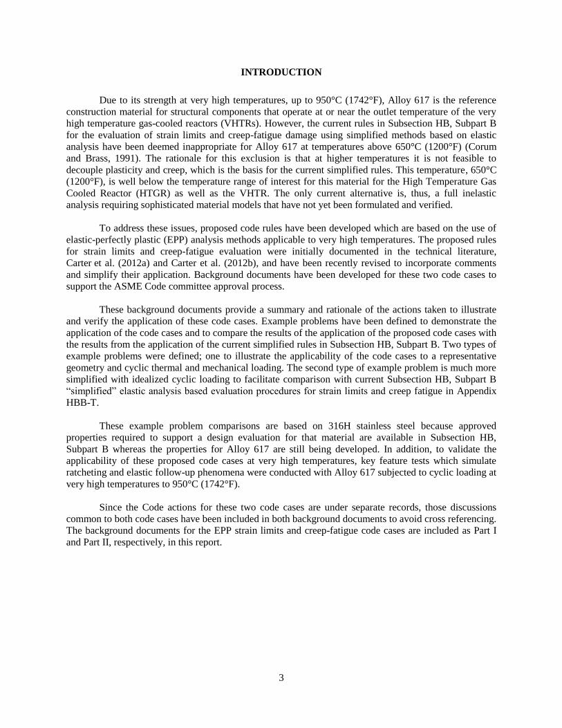
INTRODUCTION

Due to its strength at very high temperatures, up to 950°C (1742°F), Alloy 617 is the reference

construction material for structural components that operate at or near the outlet temperature of the very

high temperature gas-cooled reactors (VHTRs). However, the current rules in Subsection HB, Subpart B

for the evaluation of strain limits and creep-fatigue damage using simplified methods based on elastic

analysis have been deemed inappropriate for Alloy 617 at temperatures above 650°C (1200°F) (Corum

and Brass, 1991). The rationale for this exclusion is that at higher temperatures it is not feasible to

decouple plasticity and creep, which is the basis for the current simplified rules. This temperature, 650°C

(1200°F), is well below the temperature range of interest for this material for the High Temperature Gas

Cooled Reactor (HTGR) as well as the VHTR. The only current alternative is, thus, a full inelastic

analysis requiring sophisticated material models that have not yet been formulated and verified.

To address these issues, proposed code rules have been developed which are based on the use of

elastic-perfectly plastic (EPP) analysis methods applicable to very high temperatures. The proposed rules

for strain limits and creep-fatigue evaluation were initially documented in the technical literature,

Carter et al. (2012a) and Carter et al. (2012b), and have been recently revised to incorporate comments

and simplify their application. Background documents have been developed for these two code cases to

support the ASME Code committee approval process.

These background documents provide a summary and rationale of the actions taken to illustrate

and verify the application of these code cases. Example problems have been defined to demonstrate the

application of the code cases and to compare the results of the application of the proposed code cases with

the results from the application of the current simplified rules in Subsection HB, Subpart B. Two types of

example problems were defined; one to illustrate the applicability of the code cases to a representative

geometry and cyclic thermal and mechanical loading. The second type of example problem is much more

simplified with idealized cyclic loading to facilitate comparison with current Subsection HB, Subpart B

“simplified” elastic analysis based evaluation procedures for strain limits and creep fatigue in Appendix

HBB-T.

These example problem comparisons are based on 316H stainless steel because approved

properties required to support a design evaluation for that material are available in Subsection HB,

Subpart B whereas the properties for Alloy 617 are still being developed. In addition, to validate the

applicability of these proposed code cases at very high temperatures, key feature tests which simulate

ratcheting and elastic follow-up phenomena were conducted with Alloy 617 subjected to cyclic loading at

very high temperatures to 950°C (1742°F).

Since the Code actions for these two code cases are under separate records, those discussions

common to both code cases have been included in both background documents to avoid cross referencing.

The background documents for the EPP strain limits and creep-fatigue code cases are included as Part I

and Part II, respectively, in this report.

4

PART I – BACKGROUND FOR EPP STRAIN LIMITS CODE CASE

I-1. THEORETICAL BASIS

I-1.1 Development of Bounding Concepts

Carter et al. (2012) provided details of the bounding arguments to justify the use of a cyclic,

elastic, perfectly plastic ratcheting analysis to comply with code strain limits. The main points of the

argument are summarized below.

The use of bounding simplified solutions to characterize complex structural creep problems is

well established. The most widely used methods are for reference stress solutions to constant load

problems as, for example, reviewed in Goodall et.al. (1979). The bounding nature of shakedown solutions

for cyclic loading is also reviewed in Subsection HB, Subpart B. These ideas have been developed and

implemented in this document with the use of a temperature-dependent material property as an artificial

yield stress in limiting elastic-plastic calculations. This approach is common to low and high temperature

primary load design methods (Carter 2005a; 2005b), and to high temperature cyclic load designs Carter et

al. (2012a).

The use of simplified elastic-plastic analysis methods avoids the°omplexities and limitations of

the traditional ASME linear elastic stress classification design methods, particularly the current Tests in

ASME Section III, Division 5, Appendix HBB-T. The simplified methods exploit the fact that elastic-

plastic methods naturally handle the stress redistribution which is the key to stress classification schemes.

For high temperature design, creep strain and stress re-distribution occur naturally in service. The use of a

time-independent analysis to characterize these processes is not necessarily intuitively obvious. Their

justification by the judicious use of proofs based on general material models is therefore essential for

complex high temperature design and life assessment.

In order to guarantee creep strain limits based on elastic-plastic analysis, the conservatism of the

rapid cycle solution may be exploited. The physical principle here is that any stress history resulting from

an elastic analysis, or from an elastic-plastic analysis that shakes down to elastic behavior, provides an

upper bound to the creep deformation over time. The following sections give a summary of the

justification of this assertion. The background is as follows. For a given load and temperature cycle, a

number of solutions may be defined and calculated.

Elastic shakedown solution with a constant residual stress (SD).

Elastic-plastic solution for a perfectly plastic temperature dependent yield stress (CP).

An optimum elastic-plastic solution, the rapid cycle solution (RC).

Realistic steady cyclic creep solution (SC).

Limiting slow cycle or steady state creep solution (SS).

From each of these we may use the temperature and respective stress histories to calculate creep

strain rates, work done by boundary forces and energy dissipation rates over the volume. These may be

compared and ranked. From this, a bounding cyclic solution associated with a simplified elastic-plastic

analysis method may be identified.

5

I-1.2 Limiting Solutions

Consider a general structural problem where cyclic mechanical and thermal loads with the same

period T have been defined. The elastic solution is ( )e t .

The steady state (SS) solution is defined by the stress distribution ss such that the creep steady

state strain is kinematically admissible. This solution represents the steady loading case after stress

redistribution or the limiting case of very slow cycles.

The steady cyclic (SC) solution is the realistic limiting cyclic state with cyclic stress history

( ) ( )sc sct t T (1)

where T = cycle period, and kinematically admissible cyclic strain increments and displacement

increments.

The shakedown (SD) solution is not unique and refers to any elastic solution with a constant

residual stress field

( ) ( )e

sd t t (2)

The elastic rapid cyclic (RC) solution is the optimum shakedown solution and is the most

conservative physically achievable cyclic solution.

The elastic rapid cycle solution is defined by the constant residual stress rc such that strain

increments calculated over the cycle are kinematically admissible.

The plastic rapid cyclic (CP) solution is more general than the elastic rapid cycle which is only

valid within the shakedown limit. The plastic rapid cycle solution will generally have elastic and plastic

regions. In the elastic region the creep strain increments c are kinematically admissible as in the

previous case. In the plastic zone, the stress history is unique, and so the rapid cycle solution is the same

as the cyclic plastic solution.

The proposed method makes use of a cyclic plastic (CP) solution, which will provide an upper

bound to energy, work, strains and displacements for the other solutions mentioned above.

I-1.3 Energy and Work Bounds

This section is a summary of results obtained in Goodall et al. (1979) and Carter (2005a; 2005b).

The convexity of the yield, creep and energy dissipation functions may be used to obtain work bounds as

follows:

For mechanical loading the work W done by boundary forces over a cycle for these cases is

ordered as follows:

CP RC SC SSW W W W (3)

For combined thermal-mechanical loading, the bounding statement is in terms of energy

dissipation D over the cycle:

6

CP RC SC SSD D D D (4)

The key part of these inequalities for the simplified method used in the herein is the connection

between any cyclic plasticity solution CP and the real steady cyclic solution SC. We will use the most

advantageous cyclic plasticity solution, with the lowest stress histories and energy dissipation D over the

cycle, that does not ratchet, to bound the real steady cyclic strain accumulation.

In the analyses that follow, any elastic, perfectly plastic analysis using an artificial (“pseudo”)

yield stress derived from creep data, which does not ratchet, represents a “CP” case in inequalities (3) and

(4). The greater the time used in defining the pseudo yield stress, the more likely the analysis will give a

ratcheting result. With trial and error, it is possible to maximize the time to give a solution which does not

ratchet and so complies with the strain limits. This would provide the “RC” solution in inequalities (3)

and (4).

Table I-1 shows the nature of the possible bounds and the increasing difficulty of the proofs as

loading and material models become more general. For example, for cyclic mechanical loading, bounds to

external work may be calculated. For cyclic thermal-mechanical loading, bounds to internal energy

dissipation, not to external work, may be calculated.

Table I-1. Nature of work bounds for increasing different levels of problem complexity.

Cyclic load types Material Model

Creep Creep-plasticity

Mechanical External work External work

Thermal-

mechanical

Internal energy

dissipation

Deformation/work bound proved herein

For the most general case of thermal-mechanical loading on a creep-plasticity material, the bound

is justified using the qualitative argument below. More detail is available in Carter (2005a; 2005b). The

argument used for the general case of thermal-mechanical loading and creep-plasticity is based on the

self-evident assumption for a structure under general loading:

Reducing the perfectly plastic yield stress does not reduce the deformation.

Applied to the plastic rapid cycle solution, this statement means that the cyclic increment in

deformation of a structure is not reduced if the yield stress is reduced, all other factors being unchanged.

Therefore, if the yield stress is reduced to the point where ratcheting in a cyclic problem is imminent, then

the cyclic incremental deformation is not less than for the original yield stress. Therefore, the energy

dissipation and deflection for the reduced yield stress case provides an upper bound of the energy

dissipation and deflection in the original cases. This is the justification of the rapid cycle deformation

reference stress. This may be expressed as follows.

Consider the lowest value of the yield stress, ref , for which the ratcheting displacement

0p

cpu (5)

7

The creep energy dissipation over the cycle is less than the energy dissipation rate associated with

ref integrated over the volume and cycle.

In terms of the creep energy dissipation rate

cD (6)

this idea is expressed by

( ) ( )rc rc refD D dVdt D VT (7)

This is equivalent to the statement that the rapid cycle reference stress defining structural energy

dissipation and deformation is the lowest value of the yield stress for which the structure does not ratchet.

The strain limits code case exploits the rapid cycle concept to define a temperature dependent

“pseudo” yield stress incorporating the desired strain limit. Non-ratcheting in a conventional analysis

implies that the strain limit used to define the pseudo yield stress is satisfied.

I-2 OUTLINE OF EPP STRAIN LIMITS CODE CASE

A draft of the proposed Strain Limits Code Case is included in I-Appendix B. This code case is

intended as an alternative to the rules in HBB-T-1320, Satisfaction of Strain Limits Using Elastic

Analysis, and in HBB-T-1330, Satisfaction of Strain Limits Using Simplified Inelastic Analysis. It also

includes provisions from HBB-T-1710, Special Strain Requirements at Welds. There are five parts to the

code case and an appendix.

The objective is to comply with the Division 5, Appendix HBB-T requirements for inelastic

strains, namely:

i) Strain averaged through the thickness, 1%.

ii) Strains at the surface, due to an equivalent linear distribution of strain through the thickness,

2%.

iii) Local strains at any point, 5%.

These requirements are met by using an average, or reference, limit of 1% to define a general

ratcheting stress limit. For the case of pure bending in a uniform section, this implies a 2% limit on the

extreme fire strain.

A procedure to determine follow-up effects is used in conjunction with a local strain limit,

including follow-up effects, of 5%.

Part 1, General Requirements, describes the overall elastic-perfectly plastic ratcheting analysis

and provides a general definition of the pseudo yield strength used in this code case.

Part 2, Load Definition, identifies the manner in which loads are categorized and grouped for this

application. Code Case procedure requires that a composite cycle be defined which encompasses the

critical features of the individually defined cycles. The reason for this is that the elastic perfectly plastic

methodology used in the code case bounds the long term response independent of the number of applied

cycles. In this respect it is similar to the current simplified rules in Subsection HB, Subpart B.

8

Two sets of conditions are defined; one set for Service Levels A and B and the other for Service

Levels A and C. A feature of the proposed code case is that, unlike the current version of Subsection HB,

Subpart B, the worst case combinations of Service Level A and B do not need to be combined directly

with Service Level C. The rationale for this is that in accordance with the definition of Service Levels,

shutdown for inspection and repair or replacement is required after a Level C event whereas the reactor

system may resume planned operation after Level A and B events. The number of Level C events is

limited as it is in the lower temperature Division 1, Subsection NB rules, but, unlike the NB rules,

assessment of the high temperature displacement controlled failure modes, strain limits and creep-fatigue,

is required to guard against creep damage not measurable externally which might contribute to restraints

on the remaining life when subjected to subsequent Level A and B conditions.

Part 3, Numerical Model, specifies that the finite element model used in the analysis (The code

case is based on the use of FEA) should accurately represent the component geometry and loading

conditions, transient and steady state, including details such as local stress risers and local thermal

stresses.

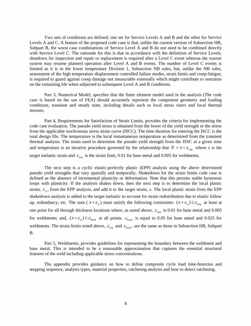
Part 4, Requirements for Satisfaction of Strain Limits, provides the criteria for implementing the

code case evaluation. The pseudo yield stress is obtained from the lower of the yield strength or the stress

from the applicable isochronous stress strain curve (ISCC). The time duration for entering the ISCC is the

total design life. The temperature is the local instantaneous temperature as determined from the transient

thermal analysis. The strain used to determine the pseudo yield strength from the ISSC at a given time

and temperature is an iterative procedure governed by the relationship that 0 avgx where x is the

target inelastic strain and avg is the strain limit, 0.01 for base metal and 0.005 for weldments.

The next step is a cyclic elastic-perfectly plastic (EPP) analysis using the above determined

pseudo yield strengths that vary spatially and temporally. Shakedown for the strain limits code case is

defined as the absence of incremental plasticity or deformation. Note that this permits stable hysteresis

loops with plasticity. If the analysis shakes down, then the next step is to determine the local plastic

strain, p , from the EPP analysis, and add it to the target strain, x. The local plastic strain from the EPP

shakedown analysis is added to the target inelastic to account for strain redistribution due to elastic follow

up, redundancy, etc. The sum ( px ) must satisfy the following constraints: ( )p avgx at least at

one point for all through thickness locations where, as noted above, avg is 0.01 for base metal and 0.005

for weldments; and, ( )p localx at all points. local is equal to 0.05 for base metal and 0.025 for

weldments. The strain limits noted above, avg and local , are the same as those in Subsection HB, Subpart

B.

Part 5, Weldments, provides guidelines for representing the boundary between the weldment and

base metal. This is intended to be a reasonable approximation that captures the essential structural

features of the weld including applicable stress concentrations.

The appendix provides guidance on how to define composite cycle load time-histories and

stepping sequence, analysis types, material properties, ratcheting analysis and how to detect ratcheting.

9

I-3 EXAMPLE PROBLEMS

There are two categories of example problems. The first category is a representative example

which demonstrates the application of the code case(s) to a representative geometry with loading

conditions representative of those which might be encountered in real design applications. The second

category is simplified geometries and loading conditions to facilitate comparison with the current rules in

Subsection HB, Subpart B.

I-3.1 Representative Example Problem

I-3.1.1 Input parameters

The following discussion is abstracted from a much more detailed report by Hollinger and Pease

(2014).

There were considerable analytic studies of different trial configurations and loading conditions.

The goal was to generate an example that would exercise relevant features of the strain limits and creep-

fatigue code cases with significant loading conditions and yet still be able to show compliance, at least for

some loadings. As noted above, the same configuration and loadings were used for both the strain limits

and creep-fatigue code cases.

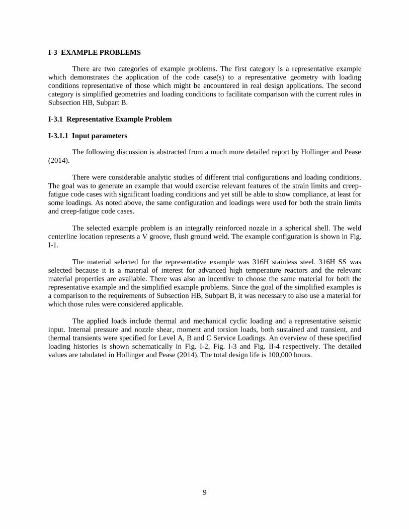
The selected example problem is an integrally reinforced nozzle in a spherical shell. The weld

centerline location represents a V groove, flush ground weld. The example configuration is shown in Fig.

I-1.

The material selected for the representative example was 316H stainless steel. 316H SS was

selected because it is a material of interest for advanced high temperature reactors and the relevant

material properties are available. There was also an incentive to choose the same material for both the

representative example and the simplified example problems. Since the goal of the simplified examples is

a comparison to the requirements of Subsection HB, Subpart B, it was necessary to also use a material for

which those rules were considered applicable.

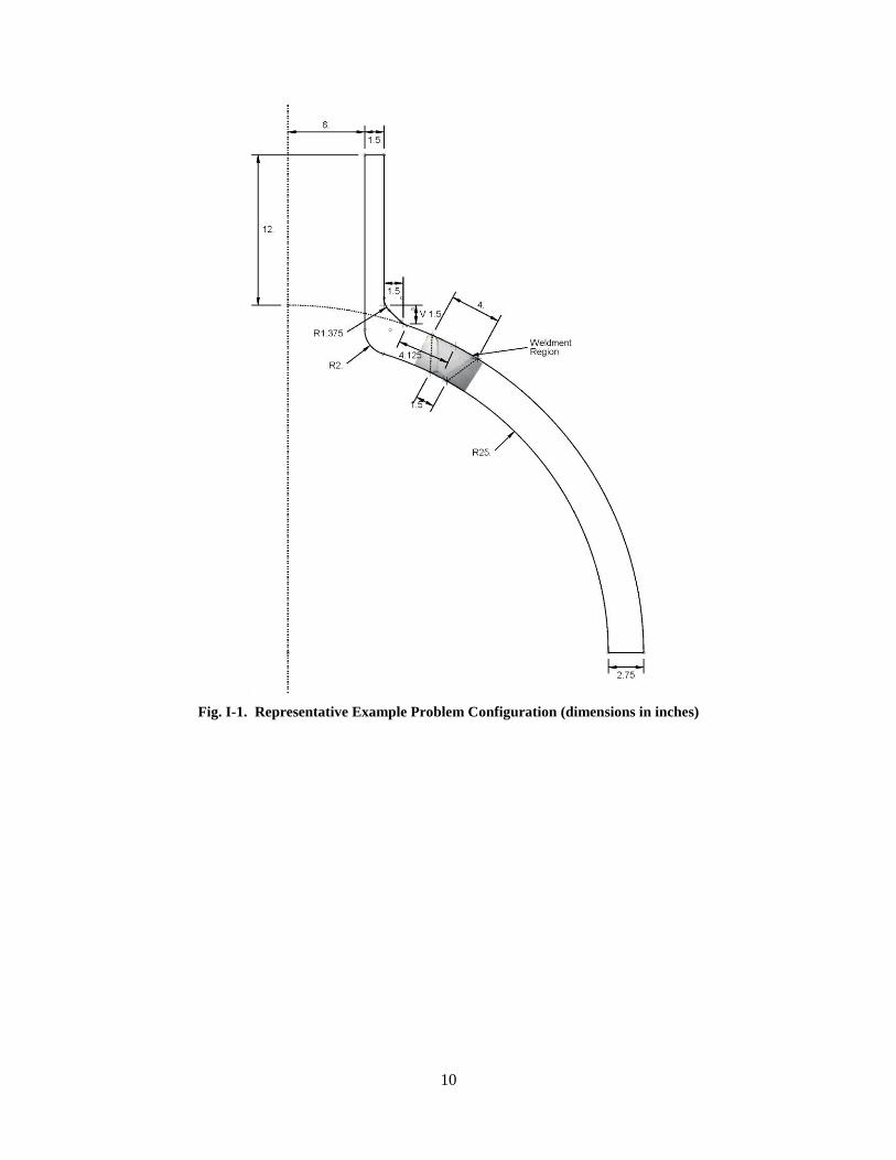
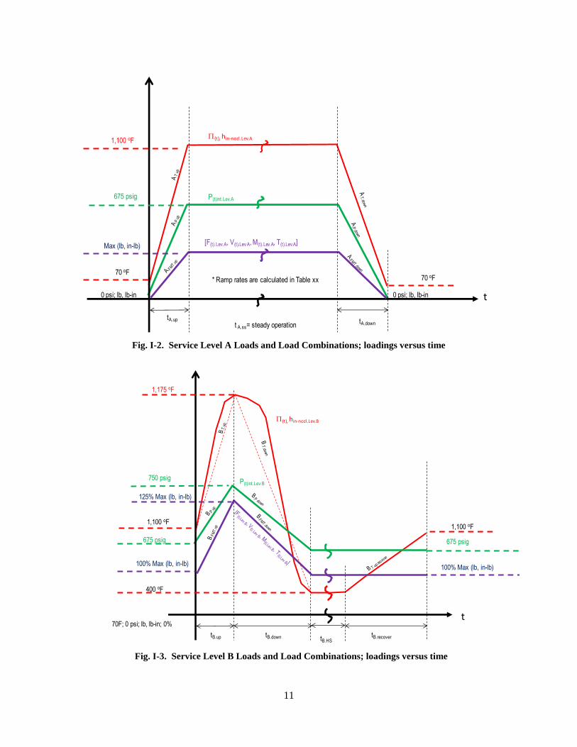
The applied loads include thermal and mechanical cyclic loading and a representative seismic

input. Internal pressure and nozzle shear, moment and torsion loads, both sustained and transient, and

thermal transients were specified for Level A, B and C Service Loadings. An overview of these specified

loading histories is shown schematically in Fig. I-2, Fig. I-3 and Fig. II-4 respectively. The detailed

values are tabulated in Hollinger and Pease (2014). The total design life is 100,000 hours.

10

Fig. I-1. Representative Example Problem Configuration (dimensions in inches)

11

Fig. I-2. Service Level A Loads and Load Combinations; loadings versus time

Fig. I-3. Service Level B Loads and Load Combinations; loadings versus time

P(t)int.Lev.A

[F(t).Lev.A, V(t).Lev A, M(t).Lev.A, T(t).Lev.A]

t

tA.up

1,100 oFP(t), hin-nozl.Lev.A

675 psig

0 psi; lb, lb-in

70 oF

Max (lb, in-lb)

t A.ss= steady operation

* Ramp rates are calculated in Table xx 70 oF

0 psi; lb, lb-in

tA.down

t

tB.up

1,175 oF

P(t), hin-nozl.Lev.B

750 psig

675 psig

1,100 oF

100% Max (lb, in-lb)

1,100 oF

675 psig



P(t)int.Lev.B

70F; 0 psi; lb, lb-in; 0%

400 oF

tB.down tB.HStB.recover

12

Fig. I-4. Service Level C Loads and Load Combinations; loadings versus time

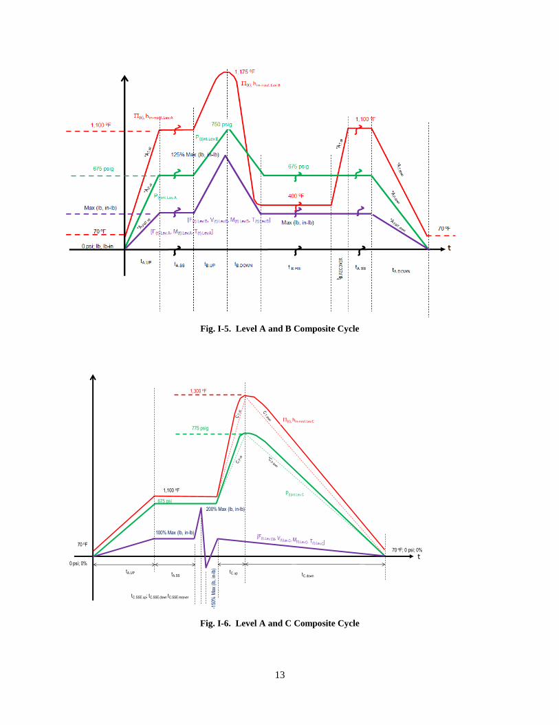
From these specified loading conditions, the Code Case procedure requires that a composite cycle

be defined which encompasses the critical features of the individually defined cycles. The reason for this

is that the elastic perfectly plastic methodology used in the code case bounds the long term response

independent of the number of applied cycles. In this respect it is similar to the current simplified rules in

Subsection HB, Subpart B. The resultant composite cycle definition is shown in Fig. I-5 and Fig. I-6.

tC.up

1,300 oF

P(t), hin-nozl.Lev.C

775 psig

675 psi

1,100 oF

70 oF; 0 psi; 0%

P(t)int.Lev.C

tC.down

t


-150% Max (lb, in-lb)

tC.SSE.up; tC.SSE.down tC.SSE.recover


13

Fig. I-5. Level A and B Composite Cycle

Fig. I-6. Level A and C Composite Cycle

tC.up

1,300 oF


775 psig

675 psi

1,100 oF

70 oF; 0 psi; 0%

P(t)int.Lev.C

tC.down

t


-150

% M

ax (l

b, in

-lb)



0 psi; 0%

70 oF

tA.UP tA.SS

14

Note that two sets of conditions are defined; one set for Service Levels A and B and the other for

Service Levels A and C. A feature of the proposed code case is that, unlike the current version of

Subsection HB, Subpart B, the worst case combinations of Service Level A and B do not need to be

combined directly with Service Level C. The rationale for this is that in accordance with the definition of

Service Levels, shutdown for inspection and repair or replacement is required after a Level C event

whereas the reactor system may resume planned operation after Level A and B events. The number of

Level C events is limited as it is in the lower temperature Division 1, Subsection NB rules, but, unlike the

NB rules, assessment of the high temperature displacement controlled failure modes, strain limits and

creep-fatigue, is required to guard against creep damage not measurable externally which might

contribute to restraints on the remaining life when subjected to subsequent Level A and B conditions.

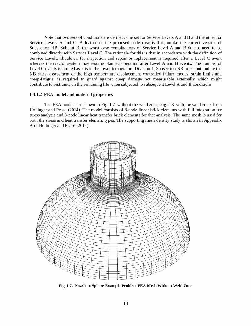
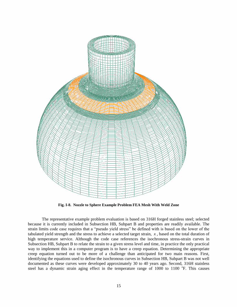
I-3.1.2 FEA model and material properties

The FEA models are shown in Fig. I-7, without the weld zone, Fig. I-8, with the weld zone, from

Hollinger and Pease (2014). The model consists of 8-node linear brick elements with full integration for

stress analysis and 8-node linear heat transfer brick elements for that analysis. The same mesh is used for

both the stress and heat transfer element types. The supporting mesh density study is shown in Appendix

A of Hollinger and Pease (2014).

Fig. I-7. Nozzle to Sphere Example Problem FEA Mesh Without Weld Zone

15

Fig. I-8. Nozzle to Sphere Example Problem FEA Mesh With Weld Zone

The representative example problem evaluation is based on 316H forged stainless steel; selected

because it is currently included in Subsection HB, Subpart B and properties are readily available. The

strain limits code case requires that a “pseudo yield stress” be defined with is based on the lower of the

tabulated yield strength and the stress to achieve a selected target strain, x , based on the total duration of

high temperature service. Although the code case references the isochronous stress-strain curves in

Subsection HB, Subpart B to relate the strain to a given stress level and time, in practice the only practical

way to implement this in a computer program is to have a creep equation. Determining the appropriate

creep equation turned out to be more of a challenge than anticipated for two main reasons. First,

identifying the equations used to define the isochronous curves in Subsection HB, Subpart B was not well

documented as these curves were developed approximately 30 to 40 years ago. Second, 316H stainless

steel has a dynamic strain aging effect in the temperature range of 1000 to 1100 oF. This causes

16

discontinuous changes in creep rate which distorts the pseudo yield strength as shown in Appendix B of

Hollinger and Pease (2014).

I-3.1.3 Methodology

Two types of analyses are run for each set of composite cycles. A transient heat transfer analysis

is performed to establish the temperature field in the vessel throughout the composite cycle. A

representative FEA plot is shown below, Fig. I- 9, illustrating the temperature distribution at the end of

the Service Level B peak up ramp to 1175 oF.

Fig. I- 9. Level B Peak Up (1175 oF)

Stress analyses are performed with the time dependent temperature field results from the heat

transfer analysis to obtain the stresses and strains in the vessel due to both mechanical loads and thermal.

Note: Each cycle of a stress analysis using a "pseudo yield stress" has no direct correlation to the number

of design or fatigue cycles and is hence defined as a "pseudo-cycle". Each composite cycle is broken up

into discrete steps and when necessary limits to maximum time increments are applied to ensure that the

analysis deals with all the changes within a cycle. The step names and durations are plotted with the time

history amplitudes in Fig. I-10 and Fig. I-11

17

Fig. I-10. Level A&B Composite Cycle Steps

Fig. I-11. Level A & C Composite Cycle Steps

0.0

0.2

0.4

0.6

0.8

1.0

1.2

1.4

0

200

400

600

800

1000

1200

1400

Leve

l A: R

amp

Up

Leve

l A: S

tead

y Sta

te 1

Leve

l B: R

amp

Up

Leve

l B: P

eak U

p

(10

sec m

ax in

crem

ents)

Leve

l B: P

eak D

own

(10

sec m

ax in

crem

ents)

Leve

l B: R

amp

Down

1

Leve

l B: R

amp

Down

2

Leve

l B: R

amp

Down

3

Leve

l B: R

amp

Down

4

Leve

l B: H

old S

tate

Leve

l B: R

ecov

er

Leve

l A: S

tead

y Sta

te 2

Leve

l A: R

amp

Down

Shutd

own:

Ste

ady S

tate

Mec

han

ical

Lo

ad F

acto

r

Tem

per

atu

re, °

F

Pre

ssu

re, p

si

Temperature Pressure Mechanical Load

-2.0

-1.5

-1.0

-0.5

0.0

0.5

1.0

1.5

2.0

2.5

0

200

400

600

800

1000

1200

1400

Leve

l A: R

amp

Up

Leve

l A: S

tead

y Sta

te 1

Leve

l C: S

SE Up

Leve

l C: S

SE Dow

n

Leve

l C: S

SE Rec

over

Leve

l C: R

amp

Up

Leve

l C: P

eak U

p

(10

sec m

ax in

crem

ents)

Leve

l C: P

eak D

own

(10

sec m

ax in

crem

ents)

Leve

l C: R

amp

Down

1

Leve

l C: R

amp

Down

2

Leve

l C: R

amp

Down

3

Shutd

own:

Ste

ady S

tate

Mec

han

ical

Lo

ad F

acto

r

Tem

per

atu

re, °

F

Pre

ssu

re, p

si


18

A pseudo-cyclic analysis is performed using the restart option to analyze multiple pseudo-cycles

of a composite cycle. After the initial pseudo-cycle is analyzed, the analysis is restarted at the end of the

previous pseudo-cycle to continue with another set of composite cycle loadings. This restart process is

repeated until a sufficient number of pseudo-cycles have been reached. For the strain limits evaluation,

stress analyses are performed where the “pseudo yield stress” is adjusted based on the selected target

inelastic strains, x . Initially the target inelastic strain is selected as the averaged inelastic strain limit,

avg , (1% for base metal and 0.5% for weld metal).

With the target inelastic strain selected; a pseudo-cyclic analysis is performed where an

intermediate check is performed at the end of each pseudo-cycle. If there exists a through thickness region

where the total inelastic strain (target inelastic strain plus plastic strains) exceed the averaged inelastic

strain limit, p avgx , then the target inelastic strain, 𝑥, is reduced. Some effort is made to maximize

the region where total inelastic stains are less than the averaged inelastic strain limit before proceeding to

the next pseudo-cycle. If further reduction of 𝑥 decreases this region then the target inelastic strain

selection has been optimized. Once optimized, if there still exists a through thickness region where total

inelastic strains exceed the averaged inelastic strain limit then it is concluded that the strain limits criteria

cannot be met. Otherwise, additional pseudo-cycles are analyzed until ratcheting has ceased.

Ratcheting is evaluated at every location in the model by checking the change in plastic strain,

p , between the beginning and end of a single pseudo-cycle. Ratcheting has ceased when there is no

change in plastic strain throughout the whole model between the beginning and end of a single pseudo-

cycle.

Plastic strains are evaluated as:

2 2 2 2 2 2

. . . . . .

22 2 2

3p x p y p z p xy p yz p zx p (8)

Note: The ABAQUS output variable for this value is PEMAG.

The total inelastic strain is defined by adding the target inelastic strain, x , to the computed

plastic strains, p :

tot px (9)

The averaged strain limits are evaluated such that there exists at least one point for all through-

thickness locations that meets the following criteria:

tot avg (10)

where avg =1% for base metal regions or 0.5% for weldment regions.

The local strain limits are evaluated such that all locations meet the following criteria:

tot local (11)

19

where local =5% for base metal regions or 2.5% for weldment regions.

Section 4.1.1 is repeated for different values of x until criteria (10) and (11) have been met and

ratcheting has ceased. If no value of x meets these requirements then it is concluded that the strain limits

criteria cannot be met.

I-3.1.4 Results

Level A & B composite cycle evaluation

The FEA model without the weld zone strain limits evaluation for the Level A & B Composite

Cycle with a target base metal inelastic strain of 1% passes after two pseudo-cycles with a maximum total

inelastic strain of 1.0006%.

The FEA model with the weld zone strain limits evaluation for the Level A & B Composite cycle

with a target base metal inelastic strain of 1% and a target weldment inelastic strain of 0.5% passes after

three pseudo-cycles with a maximum total inelastic strain of 1.0009% in the base metal at the nozzle to

shell transition and 0.5% in the weldment, with no plastic strain in the weldment.

Level A & C composite cycle evaluation

The base metal only strain limits evaluation for the Level A & C Composite Cycle does not pass.

With an optimized target base metal inelastic strain of 0.60%, the region of total inelastic strains less than

the average strain limit is maximized, but after two pseudo-cycles the total inelastic strain near the region

of where shakedown would occur is well over the 1.0% limit.

Since the base metal only evaluation did not pass for the Level A & C Composite Cycle it is

concluded that the model with weldment evaluation will not pass either, and is thus not evaluated.

I-3.2 Strain Limits Code Case to Subsection HB, Subpart B Comparison

The overall goal of this phase is to assess the design margins in the EPP methodology. This is

accomplished through the use of simplified example problem solutions which include comparison to

current NH procedures. Simplified examples are used to avoid the complexities of Subsection HB,

Subpart B simplified procedures, particularly when applied to representative geometries and loading.

I-3.2.1 Geometry and material

Case 1: Plain tube with / 4.5r t , Material: 316H stainless steel.

Case 2: Plain tube with / 3.5r t , Material: 316H stainless steel.

Case 3: Case 1 connected to Case 2, with a 3:1 external taper in wall thickness.

I-3.2.2 Strain limits evaluation – level A/B service loadings

The objective of this analysis is to calculate the maximum through wall temperature difference

for tubes #1 and #2 and to calculate the operating time required to satisfy the 1% strain limits. The target

life is 100,000 hours.

These calculations will be based on a design pressure of 1.3 ksi in both tubes, and a temperature

cycle defined by a uniform 1075 oF to the temperature distributions defined below.

20

For tube #1, consider steady state metal temperatures defined by 1200 oF in the bore, and 1075

oF

on the OD. Using the formula for thermal stress in a tube with through-wall heat flux in Pitts and Sissom

(1998), the radial steady state heat flux for these temperatures is 105 BTU/in/in/hour. The steady state

bore temperature in tube #2 for this heat flux and the 1075 oF tube OD temperature is 1235

oF. A heat flux

cycle from zero to 105 BTU/in/in/hour is used in the following steady state thermal-mechanical

calculations.

Thermal-mechanical properties at 1100 oF are given in Table I-2 Thermal and mechanical elastic

stresses are obtained from thick-walled pipe formulas in Roark and Shaum.

Table I-2. Thermo-Mechanical Properties of TP316H at 1100

oF

Spec. Heat

BTU/(lb⋅ oF)

Conductivity

BTU/(hr⋅in⋅°F)

Exp.

Coefficient

in/in/oF

Young's

Modulus

ksi

143.14 1.1055 1.029E-05 21928

I-3.2.3 Strain limits evaluation – Subsection HB, Subpart B simplified methods

Table I-3 gives results of Tests B1 and B2; these are used to determine the strain limits and the

times to exceed the 1% limit for through wall average strain.

Table I-3. Summary of HBB-T-1332 Test B1 and B2 Strain Limits Calculations

HBB -T-1330 Strain

Limits

Tube 1 Tube 2

Test B1 Test B2 Test B1 Test B2

Load cases 1.3 ksi,

1200 oF - 1075 oF

1.3 ksi,

1200 oF - 1075 oF

1.3 ksi,

1235 oF - 1075 oF

1.3 ksi,

1235 oF - 1075 oF

ID Temperature F 1200 1200 1235 1235

OD Temperature F 1075 1075 1075 1075

Yield stress ksi Sy (mean hot wall

temp)

16.55 16.55 16.45 16.45

Yield stress ksi SyL (lower cycle

temp)

16.67 16.67 16.8 16.8

Pressure stress ratio X 0.41 0.41 0.39 0.39

Thermal stress 19.94 19.94 25.4 25.4

Thermal stress ratio Y 1.19 1.19 1.53 1.5

Creep stress parameter Z (s2) 0.49 0.60 0.59 0.75

Creep stress parameter Z (s1) 0.51 0.59

sigmac with factor

1.25

10.24 12.58 12.4 15.73

HBB-T-1800 B7 - B9 Hours - 1% strain 5.50E+05 1.10E+05 1.10E+05 1.40E+04

Test B2 would be necessary if there was a significant peak stress component of thermal stress.

The use of the HBB-T-1325 formula for piping thermal stress means that any peak thermal stress due to

the relatively thick sections is effectively ignored. The difference between the thermal stress from this

21

formula and the correct calculation for a thick tube (Roark and Young, 1989) is 7.5%. The NH code states

that test B1 can only be used if the peak stress is negligible. For comparison, results from both tests B1

and B2 are presented.

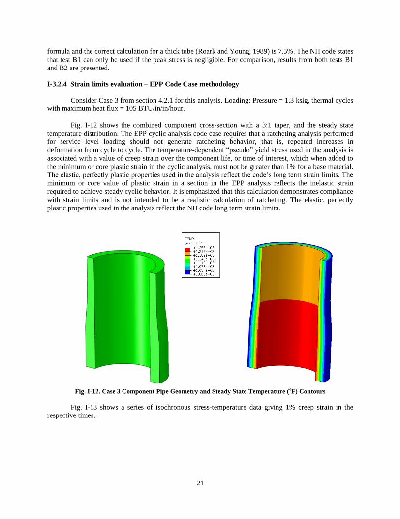
I-3.2.4 Strain limits evaluation – EPP Code Case methodology

Consider Case 3 from section 4.2.1 for this analysis. Loading: Pressure = 1.3 ksig, thermal cycles

with maximum heat flux = 105 BTU/in/in/hour.

Fig. I-12 shows the combined component cross-section with a 3:1 taper, and the steady state

temperature distribution. The EPP cyclic analysis code case requires that a ratcheting analysis performed

for service level loading should not generate ratcheting behavior, that is, repeated increases in

deformation from cycle to cycle. The temperature-dependent “pseudo” yield stress used in the analysis is

associated with a value of creep strain over the component life, or time of interest, which when added to

the minimum or core plastic strain in the cyclic analysis, must not be greater than 1% for a base material.

The elastic, perfectly plastic properties used in the analysis reflect the code’s long term strain limits. The

minimum or core value of plastic strain in a section in the EPP analysis reflects the inelastic strain

required to achieve steady cyclic behavior. It is emphasized that this calculation demonstrates compliance

with strain limits and is not intended to be a realistic calculation of ratcheting. The elastic, perfectly

plastic properties used in the analysis reflect the NH code long term strain limits.

Fig. I-12. Case 3 Component Pipe Geometry and Steady State Temperature (oF) Contours

Fig. I-13 shows a series of isochronous stress-temperature data giving 1% creep strain in the

respective times.

22

Fig. I-13. 316H SS Isochronous 1% Inelastic Strain Data

Fig. I-14, Fig. I-15, Fig. I-16 and Fig. I-17 show results of ratcheting analyses. Ratcheting is

indicated by a clear increase in strain from cycle to cycle. Strain limits require consideration of cyclic

strain accumulation as well as the strain accumulated in order to achieve the steady cyclic state. Fig. I-14

and Fig. I-15 show no ratcheting with the basic design loads. Fig. I-16 and Fig. I-17 show ratcheting (that

is, failure to demonstrate strain limits) for the tube intersection. Fig. I-18 shows that the plain tubes can

satisfy the strain limits criterion on their own, with a factor of 1.2 on pressure and heat flux. Note that this

factor changes the magnitude of stress and increases temperatures.

Fig. I-14. Non Ratcheting Strain Histories for Tube 2 with Design and Thermal Stress x 1.0. Cyclic strain (x)

= 0.095. y = Core strain (y) = 0.0001. 1% Limit Demonstrated.

23

Fig. I-15. Contour Plot of Radial Deflection Differences Between Cycles. Design Pressure and Thermal

Loading x 1. Apparent Differences not Numerically Significant. Ratcheting not Indicated.

Fig. I-16. Ratcheting Strain Histories for Tube 2 Intersection with Design and Thermal Stress x 1.2. Strain

Limits Not Met.

24

Fig. I-17. Contour Plot of Radial Deflection Differences Between Cycles. Design Pressure and

Thermal Stress x 1.2. Ratcheting in Intersection Indicates Strain Limits are Not Met.

25

Fig. I-18. Non-Ratcheting Strain Histories for Tube 1 and Tube 2 Respectively. From the Component

Model. Design and Thermal Stress x 1.2. Cyclic Strain (x) = 0.096, y = Core Strain (y) < 0.0002. 1%

Limit Demonstrated.

Table I-4 summarizes results of ratcheting calculations on plain tubes and tapered joined tubes

expressed as margins on design conditions which generate 1% inelastic strain in 1 x 105 hours.

Table I-4. Results of Ratcheting Calculations of Plain Tubes and Tapered Joined Tube

Case 1. Thinner

tube

Case 2. Thicker

tube

Case 3. Joined

tubes

Margins on design cycles

shown to satisfy strain limits

1.2 1.2 1.0

26

I-4 EXPERIMENTAL RESULTS COMPARISON

I-4.1 Two-Bar Test Evaluation

The two-bar test concept was initiated a number of years ago to support high temperature design

criteria for the Clinch River Breeder Reactor (CRBR). The goal of the two-bar test is to simulate the

thermal ratcheting failure mode which is the basis of the strain limits design criteria in Subsection HB,

Subpart B of Section III. This type of testing was originally performed on 2¼Cr-1Mo steel (Swindeman

et al., 1982) to support the verification of the recommended constitutive equations for liquid metal-cooled

fast breeder reactor (LMFBR) applications. However, the current very high temperature two-bar test

results on Alloy 617 will also, initially, be used to validate the newly proposed simplified methodology

for assessment of strain limits at very high temperatures where the current NH methodology has been

deemed inappropriate for Alloy 617.

In the two-bar test methodology, the two bars are alternately heated and cooled under sustained

axial loading to generate ratcheting. A sustained hold time is introduced at the hot extreme of the cycle to

capture the accelerated ratcheting and strain accumulation due to creep. Since the boundary conditions are

a combination of strain control and load control it is necessary to use two coupled servo-controlled testing

machines to achieve the key features of the two-bar representation of actual component behavior.

In this method, the two bars can be viewed as specimens taken out of a tubular component across

the wall thickness representing the inner wall element and the outer wall element. During operation, a

constant mean stress is applied on to the tube represented by the two bars. A schematic of the two-bar

system is shown in Fig. I-19(a). There are two boundary conditions to tie these two bars together in order

to represent the real component loading conditions. As shown in Fig. I-19(b), the two bars experience

equal total displacements at all time, and the total load applied to the two bars is constant.

(a) (b)

Fig. I-19. Schematic of Two-bar thermal ratcheting condition (a) and the equivalent boundary

conditions of the two bars (b)

Conceptually, the two bars in parallel can be thought of as representing the inner and outer wall

of a pressurized cylinder subjected to a cyclic through wall temperature gradient, e.g. a Bree type

geometry.

The two-bar tests on Alloy 617 were performed by Wang et al. (2013). Fig. I-20 shows the

temperature versus time histogram which was used in this study. Fig. I-21 shows the resulting strain

Rigid

Rigid

Bar 1

Temp. 1

Bar 2 Temp. 2

Constant total load,

Bar 1 Temp. 1

Bar 2 Temp. 2

27

history under several constant applied loads. A moderate tensile load for a 4 ksi average stress in the bars

results in accelerated tensile elongation and the same load in compression generates an even higher

compressive strain per cycle. These initial scoping tests were conducted at a relatively slow heating and

cooling rate of 5 oC/min (9

oF/min).

Fig. I-20. Temperature vs. time histogram for two-bar thermal ratcheting experiments on Alloy 617

Fig. I-21. The maximum and the minimum total strains in the two bars at temperature range 800ºC to 950ºC

(heating and cooling rates were 5 oC/min).

Further two-bar test results were conducted with a more severe temperature difference and higher

heating and cooling rate, 30 oC/min (54

oF/min). These test results showed an anomaly when compared to

strain limit predictions based on the EPP strain limits code case. Fig. I-22 is a plot of two-bar test data

compared with two methods for predicting allowable loading that would result in 1% or less creep strain.

The vertical axis is the time delay from point 3 on Fig. I-20, the initiation of the thermal down ramp in bar

1, and point 5, the initiation of the thermal down ramp in bar 2. The tested temperature range was 650 ºC

to 950 ºC (1202 ºF to 1742 ºF). The total temperature change and ramp rates are the same for the tests

Time

Tem

per

atu

re

Bar 1

Bar 2

Bar 1 & Bar 2 Bar 2

Bar 1

-0.02

0

0.02

0.04

0.06

0.08

0.1

0 5 10 15 20 25 30 35 40

To

tal

stra

in

Cycle number

Bar 1-Max strain Bar 1-Min strain

Bar 2-Max strain Bar 2-Min strain

σm=0.5ksi

σm=-4.2ksi

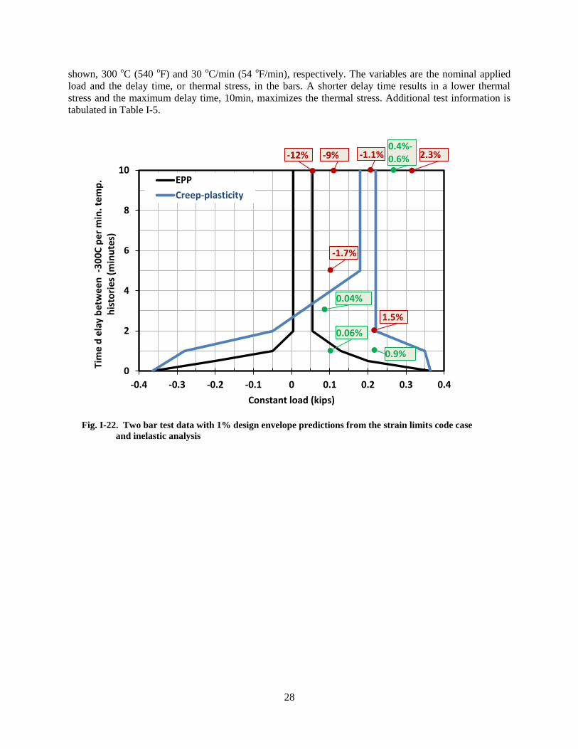
28

shown, 300 oC (540

oF) and 30

oC/min (54

oF/min), respectively. The variables are the nominal applied

load and the delay time, or thermal stress, in the bars. A shorter delay time results in a lower thermal

stress and the maximum delay time, 10min, maximizes the thermal stress. Additional test information is

tabulated in Table I-5.

Fig. I-22. Two bar test data with 1% design envelope predictions from the strain limits code case

and inelastic analysis

0

2

4

6

8

10

-0.4 -0.3 -0.2 -0.1 0 0.1 0.2 0.3 0.4

Tim

e d

ela

y b

etw

ee

n -

30

0C

pe

r m

in. t

em

p.

his

tori

es

(min

ute

s)

Constant load (kips)

EPP

Creep-plasticity

0.06%

0.04%

-1.7%

-12% -9% -1.1% 0.4%-0.6% 2.3%

0.9%

1.5%

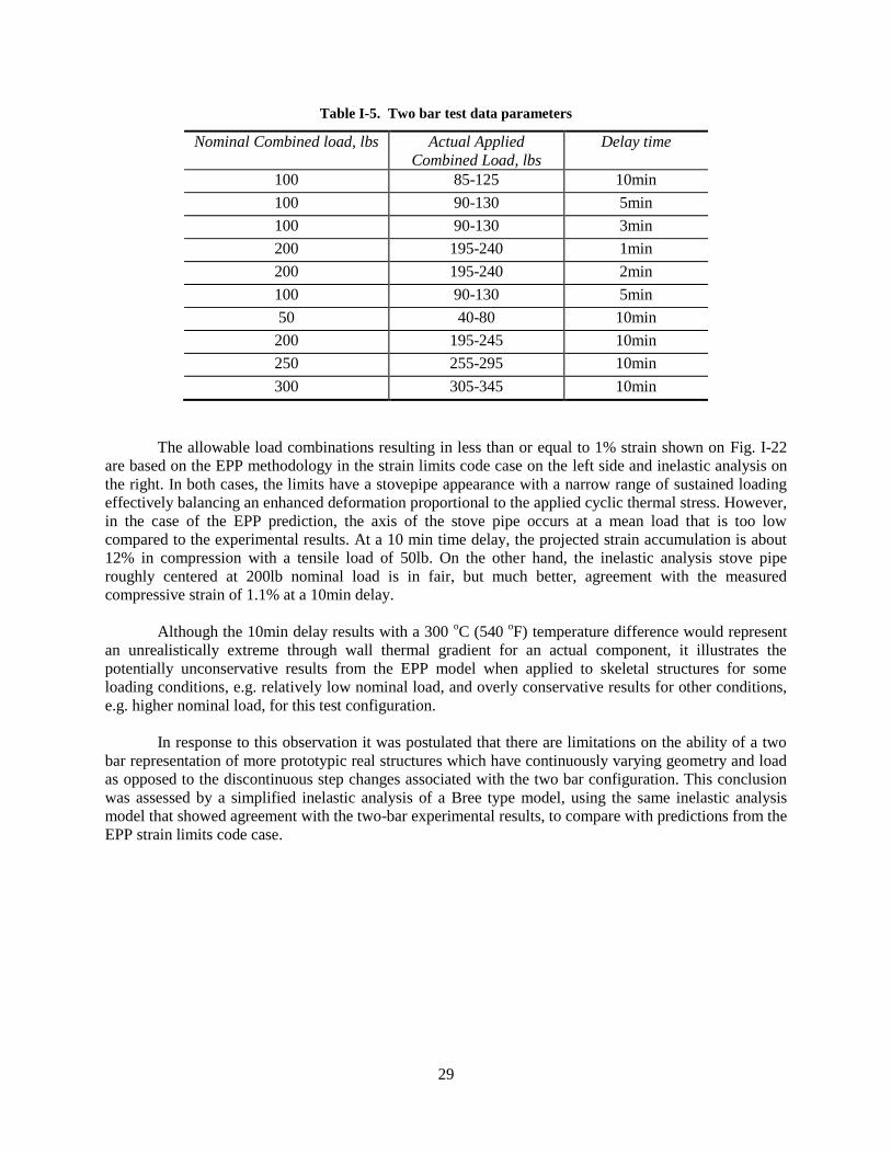
29

Table I-5. Two bar test data parameters

Nominal Combined load, lbs Actual Applied

Combined Load, lbs

Delay time

100 85-125 10min

100 90-130 5min

100 90-130 3min

200 195-240 1min

200 195-240 2min

100 90-130 5min

50 40-80 10min

200 195-245 10min

250 255-295 10min

300 305-345 10min

The allowable load combinations resulting in less than or equal to 1% strain shown on Fig. I-22

are based on the EPP methodology in the strain limits code case on the left side and inelastic analysis on

the right. In both cases, the limits have a stovepipe appearance with a narrow range of sustained loading

effectively balancing an enhanced deformation proportional to the applied cyclic thermal stress. However,

in the case of the EPP prediction, the axis of the stove pipe occurs at a mean load that is too low

compared to the experimental results. At a 10 min time delay, the projected strain accumulation is about

12% in compression with a tensile load of 50lb. On the other hand, the inelastic analysis stove pipe

roughly centered at 200lb nominal load is in fair, but much better, agreement with the measured

compressive strain of 1.1% at a 10min delay.

Although the 10min delay results with a 300 oC (540

oF) temperature difference would represent

an unrealistically extreme through wall thermal gradient for an actual component, it illustrates the

potentially unconservative results from the EPP model when applied to skeletal structures for some

loading conditions, e.g. relatively low nominal load, and overly conservative results for other conditions,

e.g. higher nominal load, for this test configuration.

In response to this observation it was postulated that there are limitations on the ability of a two

bar representation of more prototypic real structures which have continuously varying geometry and load

as opposed to the discontinuous step changes associated with the two bar configuration. This conclusion

was assessed by a simplified inelastic analysis of a Bree type model, using the same inelastic analysis

model that showed agreement with the two-bar experimental results, to compare with predictions from the

EPP strain limits code case.

30

I-5 ANALYTICAL COMPARISONS

I-5.1 Background

As discussed above, two-bar Alloy 617 high temperature ratcheting tests were performed to test

predictions of proposed simplified elastic, perfectly plastic (EPP) analysis methods. Differences between

tests and the simplified method predictions led to the use of detailed inelastic analyses which were more

successful in explaining the two-bar cyclic ratcheting behavior. The objective of this task is to determine

if there are differences between the predictions from these two methods for a typical plant pressure part,

such as a pressurized pipe subject to cyclic through-wall thermal loading. A case was analyzed with

stresses and cycles for the pipe problem similar in magnitude to those for the two-bar tests. Included is

background to the use of a simplified elastic, perfectly plastic analysis method for the assessment of strain

limits.

I-5.2 Bounding Theories

The basis for simplified methods is generally expressed in terms of energy bounding theorems.

There is a “hierarchy” of bounding concepts which reflects the trade-off between problem complexity and

bounding accuracy.

Problems with mechanical load cycles may be bounded by external work bounds.

Problems with thermal and mechanical load cycles may be bounded by internal energy

dissipation. This is generally more conservative than for purely mechanical problems, since high

internal energy dissipation may be associated with zero net deflection.

In both cases, the opportunity for a simplified analysis arises from the use of the “rapid cycle”

concept. Rapid cycles have no creep relaxation during the cycle, but generally have the most

advantageous residual stress system which ensures that deformation rates over the cycle are as low as

possible.

It is clear that “average” quantities in these arguments, such as external work, are important. This

may point to the reason why the application to the two-bar problem is more difficult than for continuum

problems.

In terms of deformation and strain accumulation over time, rapid cycles are more conservative

than slow cycles. Therefore, if strain limits can be demonstrated for rapid cycles, slower cycles with

relaxation will also satisfy the strain limits.

The use of elastic, perfectly plastic (EPP) analysis using an artificial or pseudo yield stress is

based on a third assumption, that reducing the yield stress in an analysis is conservative, that is,

does not reduce the deformation rates.

Thus, if the temperature-dependent “pseudo” yield stress in a rapid cyclic analysis is reduced to

the point where ratcheting is imminent, then the deformation will not be less than with the realistic yield

property. If this pseudo yield stress is based on the stress to give 1% inelastic strain, then it is possible for

stress and temperature cycles to exist everywhere in the structure which do not produce more than the 1%

inelastic strain limit in the specified time. This argument presents a possibility and is not a proof. It is

consistent with the ASME Section III, NH, Test B1 iso-strain contours within the non-ratcheting region of

the Bree diagram used in this test. There is reason to suppose that it is more applicable in a continuum

than in a skeletal structure.

31

Proofs of the work bound theorems rely on a convexity property of the creep constitutive law

which is unlikely to be a restriction or inapplicable for Alloy 617. These proofs are more straightforward

for purely time-dependent materials than for materials with creep behavior within a plastic yield surface.

A significant effort has been made to generalize the purely creep, cyclic bounding arguments to deal with

a yield surface in a creep-yielding material model. The key property for a purely time-dependent material

is that cyclic loading sets up cyclic stress histories for which creep energy dissipation is a minimum

compared with non-cyclic stress histories. For a rapid cycle with purely time-dependent behavior, the

stress history may be represented by the sum of elastic stress, plus a residual stress. The rapid cycle

residual stress is the unique value which provides a kinematically admissible cyclic creep strain increment

over the cycle. The conservative (bounding) nature of the rapid cycle only depends on a convexity

property of the inelastic strain rate constitutive law.

I-5.3 Material Properties and Pseudo Yield Stress

Fig. I-23 shows stress – inelastic strain rate plots at 1200 oF, 1500

oF and 1800

oF. These plots

were constructed by assuming a linear relationship for the correlation of time to 1% total strain of

Eno et al. (2008) for Alloy 617. It also shows a hyperbolic sine (“ksn”) model fit to these relations, with

the Abaqus constants for this model tabulated in the figure. The hyperbolic sine model for the creep strain

rate is given as

exp sinhc

nQA B

RT

(12)

Fig. I-24 shows pseudo yield stress for 1% inelastic strain accumulation in 200 hours based on the

hyperbolic sine model. The pseudo yield stress needs to be calculated for 1% inelastic strain in 200 hours.

This is done on the basis that inelastic strain is proportional to time for constant stress and temperature

loading. The only correction required is for elastic strain, since Alloy 617 does not have a defined plastic

strain at high temperatures. The pseudo yield stress shown in Fig. I-24 is used in analyses for Fig. I-22

and Fig. I-29.

Power Law

Multiplier, A 3.0158 E+25

Hyperb. Law

Multiplier, B 0.01201

Eqn. Order, n 5.7180

Activation

Energy, Q 516622

Gas Constant, R 4.619

Fig. I-23. Alloy 617 Inelastic Stress – Strain Rates and Material Model Parameters (Units: oF, hours, ksi,

BTU, lbs).

32

Fig. I-24. Alloy 617 Stress versus Temperature for Yield and 1% Inelastic Strain in 200

Hours

I-5.4 Inelastic Strain Limits and Ratcheting Analyses

Consider the problem summarized in Table I-6. A pipe is required to survive thermal cycles for

200 hours without violating a 1% inelastic strain limit. In this case, the strain limit refers to the hoop

strain in the center of the pipe wall. This reflects the requirement for a 1% inelastic strain limit on average

or membrane strain.

The first objective is to use the EPP analysis method to determine acceptable pressures (negative

and positive) for which the 1% inelastic strain limit is satisfied. The second objective is to verify the

design calculations with a detailed cyclic inelastic analysis.

The maximum through wall temperature distribution is illustrated in Fig. I-25. The criterion for

acceptable stain accumulation based on the EPP cyclic analysis requires consideration of cyclic strain

accumulation and the strain required to achieve the steady cyclic state. The inelastic strain requirement is

that cyclic strain accumulation x (which defines the pseudo yield stress) plus inelastic strain required for

re-distribution y (defined by the minimum EPP non-ratcheting analysis plastic strain in the section),

should be less than 1%.

Table I-6. Design Data

Material Pipe OD " Pipe ID " OD

Temperature

(0F)

ID

Temperature

Max. Range

(0F)

Hours

Alloy 617 14 12 1742 1202 - 1742 200

33

Fig. I-25. Through Wall Temperature Contours and Second Order Mesh

I-5.4.1 EPP ratcheting analysis

Fig. I-26 shows examples of EPP cyclic analyses, exhibiting non-ratcheting and ratcheting.

Ratcheting is indicated by a clear increase in strain from cycle to cycle. Evidence of overall non-

ratcheting is required for an acceptable design. Strain limits require consideration of cyclic strain

accumulation (x) as well as the strain accumulated in order to achieve the steady cyclic state (y). Fig. I-27

shows EPP examples with zero and non-zero plastic strain values y.

Table I-7 is a summary of EPP calculations and the cyclic and re-distribution strains, x and y,

respectively. In the one case where the y strain is non-zero, the effect on hours to guarantee the 1% limit

is not significant.

(a) (b)

Fig. I-26. Examples of Non-Ratcheting (a) and Ratcheting (b) Strain Histories

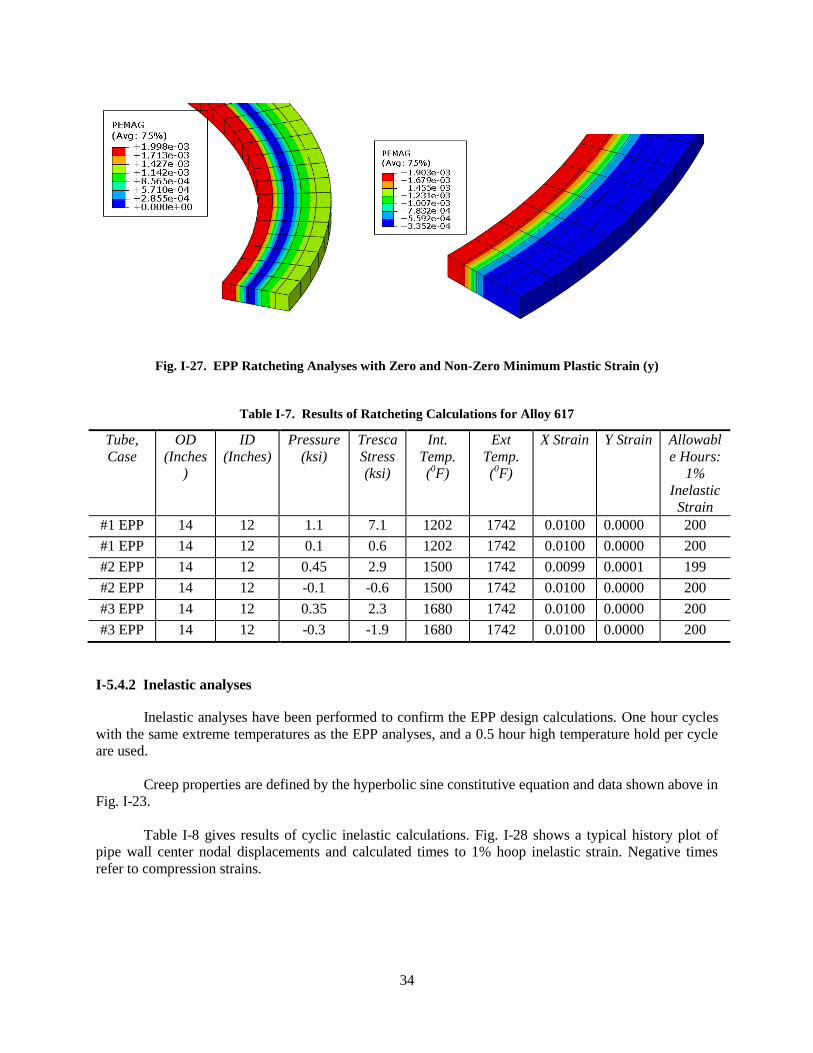
34

Fig. I-27. EPP Ratcheting Analyses with Zero and Non-Zero Minimum Plastic Strain (y)

Table I-7. Results of Ratcheting Calculations for Alloy 617

Tube,

Case

OD

(Inches

)

ID

(Inches)

Pressure

(ksi)

Tresca

Stress

(ksi)

Int.

Temp.

(0F)

Ext

Temp.

(0F)

X Strain Y Strain Allowabl

e Hours:

1%

Inelastic

Strain

#1 EPP 14 12 1.1 7.1 1202 1742 0.0100 0.0000 200

#1 EPP 14 12 0.1 0.6 1202 1742 0.0100 0.0000 200

#2 EPP 14 12 0.45 2.9 1500 1742 0.0099 0.0001 199

#2 EPP 14 12 -0.1 -0.6 1500 1742 0.0100 0.0000 200

#3 EPP 14 12 0.35 2.3 1680 1742 0.0100 0.0000 200

#3 EPP 14 12 -0.3 -1.9 1680 1742 0.0100 0.0000 200

I-5.4.2 Inelastic analyses

Inelastic analyses have been performed to confirm the EPP design calculations. One hour cycles

with the same extreme temperatures as the EPP analyses, and a 0.5 hour high temperature hold per cycle

are used.

Creep properties are defined by the hyperbolic sine constitutive equation and data shown above in

Fig. I-23.

Table I-8 gives results of cyclic inelastic calculations. Fig. I-28 shows a typical history plot of

pipe wall center nodal displacements and calculated times to 1% hoop inelastic strain. Negative times

refer to compression strains.

35

Table I-8. Inelastic Displacements and Strains

Tube, Case Pressure

(ksi)

Int. Temp

(0F)

Ext. Temp

(0F)

Step 4 Node

Disp. Ins

Step 5 Node

Disp. Ins

Hours: 1%

Inelastic Strain

#1 creep 1.2 1202 1742 0.0057825 0.005988 288

#1 creep -0.2 1202 1742 -0.0041267 -0.004358 -299

#2 creep 0.7 1500 1742 0.0029036 0.003155 247

#2 creep -0.3 1500 1742 -0.004456 -0.004768 -223

#3 creep 0.65 1680 1742 0.003062 0.00341 178

#3 creep -0.6 1680 1742 -0.002849 -0.003173 -209

Fig. I-28. Tube Radial Nodal Displacements for Tube Case #3 Negative Pressure Loading

I-5.4.3 Summary of EPP ratcheting and inelastic analyses

Fig. I-29 is a summary of all load cases with stress normalized by the mean wall temperature

yield stress at the maximum thermal stress. Design points are calculated so that the pressure load is as

close as possible to the ratchet limits based on the pseudo yield stress and the Eno et al. (2008)

correlation. Inelastic calculations have been extrapolated from the first five cycles and give lives to 1%

inelastic strain of 200 – 300 hours. The usual Bree diagram limits for ratcheting and shakedown are

shown to indicate regions of behavior. The results for zero thermal stress are based on spreadsheet

calculations, and reflect both methods.

It may be seen that that all the inelastic calculations with lives of 200 – 300 hours are less

conservative then the EPP design calculations, but not excessively so; thus the EPP methodology may be

concluded to provide a reasonable design bound for the response of representative structures with

distributed properties and temporal and spatially varying structural response.

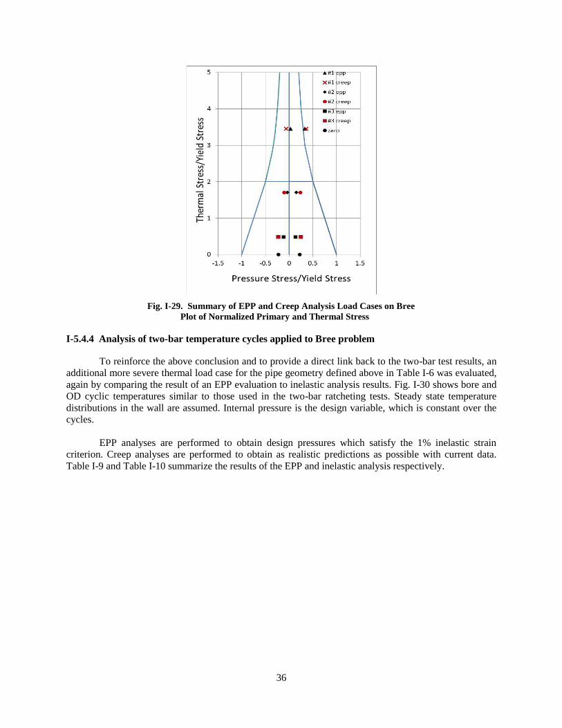
36

Fig. I-29. Summary of EPP and Creep Analysis Load Cases on Bree

Plot of Normalized Primary and Thermal Stress

I-5.4.4 Analysis of two-bar temperature cycles applied to Bree problem

To reinforce the above conclusion and to provide a direct link back to the two-bar test results, an

additional more severe thermal load case for the pipe geometry defined above in Table I-6 was evaluated,

again by comparing the result of an EPP evaluation to inelastic analysis results. Fig. I-30 shows bore and

OD cyclic temperatures similar to those used in the two-bar ratcheting tests. Steady state temperature

distributions in the wall are assumed. Internal pressure is the design variable, which is constant over the

cycles.

EPP analyses are performed to obtain design pressures which satisfy the 1% inelastic strain

criterion. Creep analyses are performed to obtain as realistic predictions as possible with current data.

Table I-9 and Table I-10 summarize the results of the EPP and inelastic analysis respectively.

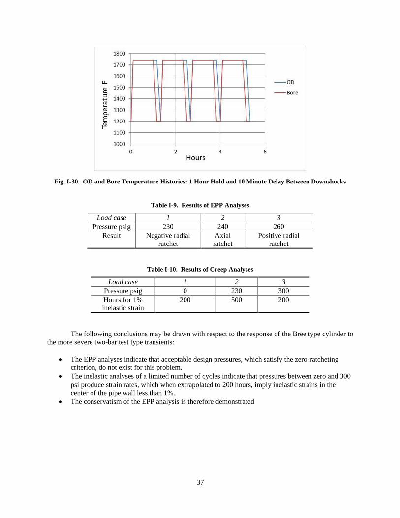
37

Fig. I-30. OD and Bore Temperature Histories: 1 Hour Hold and 10 Minute Delay Between Downshocks

Table I-9. Results of EPP Analyses

Load case 1 2 3

Pressure psig 230 240 260

Result Negative radial

ratchet

Axial

ratchet

Positive radial

ratchet

Table I-10. Results of Creep Analyses

Load case 1 2 3

Pressure psig 0 230 300

Hours for 1%

inelastic strain

200 500 200

The following conclusions may be drawn with respect to the response of the Bree type cylinder to

the more severe two-bar test type transients:

The EPP analyses indicate that acceptable design pressures, which satisfy the zero-ratcheting

criterion, do not exist for this problem.

The inelastic analyses of a limited number of cycles indicate that pressures between zero and 300

psi produce strain rates, which when extrapolated to 200 hours, imply inelastic strains in the

center of the pipe wall less than 1%.

The conservatism of the EPP analysis is therefore demonstrated

38

I-5.5 Bounding Theory Example Calculations

To date, example calculations have not been developed to illustrate the application of bounding

concepts with an analytical solution of a simplified strain limits problem. However, such calculations

have been developed for a simplified creep-fatigue problem and are documented in the creep-fatigue

background document.

I-6 SUMMARY AND CONCLUSIONS

The goal of this report is to provide a summary and rationale of the actions taken to illustrate and

verify the application of one of the two code cases developed to permit evaluation of strain limits and

creep-fatigue damage that take advantage of the unique features of elastic-perfectly plastic analysis

methods for Section III, Division 5 Subsection HB, Subpart B applications. This report focuses on the

strain limits code case. A motivating factor in developing the code cases is the restriction on the

application of current Subsection HB, Subpart B simplified methods to Alloy 617 at very high

temperature. The overall strategy is to (1) illustrate the application the code case(s) to an example

problem representative of a realistic component with realistic loading conditions, (2) compare the results

of an evaluation based on the proposed code case methods to the results from a Subsection HB, Subpart B

evaluation using an example(s) with simplified geometry and loading conditions, and (3) compare the

code case predictions with test data from key feature experiments primarily on Alloy 617 at very high

temperature simulating ratcheting and elastic follow-up phenomena.

I-6.1 Basis Of The Code Case Methodology

The basis for the proposed simplified methods is generally expressed in terms of energy bounding

theorems. There is a “hierarchy” of bounding concepts which reflects the trade-off between problem

complexity and bounding accuracy. Problems with mechanical load cycles may be bounded by external

work bounds and those with thermal and mechanical load cycles may be bounded by internal energy

dissipation. This is generally more conservative than for purely mechanical problems, since high internal

energy dissipation may be associated with zero net deflection. In both cases, the opportunity for a

simplified analysis arises from the use of the “rapid cycle” concept.

Rapid cycles have no creep relaxation during the cycle, but generally have the most advantageous

residual stress system which ensures that deformation rates over the cycle are as low as possible. In terms

of deformation and strain accumulation over time, rapid cycles are more conservative than slow cycles.

Therefore, if strain limits can be demonstrated for rapid cycles, slower cycles with relaxation will also

satisfy the strain limits.

The use of elastic, perfectly plastic (EPP) analysis using an artificial or pseudo yield stress is

based on a third assumption - that reducing the yield stress in an analysis is conservative, that is, does not

reduce the deformation rates. Thus, if the temperature-dependent “pseudo” yield stress in a rapid cyclic

analysis is reduced to the point where ratcheting is imminent, then the deformation will not be less than

with the realistic yield property. If this pseudo yield stress is based on the stress to give 1% inelastic

strain, then it is possible for stress and temperature cycles to exist everywhere in the structure which do

not produce more than the 1% inelastic strain limit in the specified time.

Note that there is no requirement for a high temperature yield property in these arguments. The

restriction on the use of current simplified methods is, essentially, that they are based on yield properties

and the separation of plasticity and creep.

39

I-6.2 Representative Example Problem

The goal of the representative example is to illustrate the code case(s) application to a realistic

geometry and loading conditions. The selected geometry is a spherical head with an integrally reinforced

nozzle with a flush ground connecting weld. The applied loads are internal pressure and shear and

moment loads on the nozzle. Cyclic and sustained loading conditions are evaluated with imposed thermal

transients. The material is 316H stainless steel.

The implementation evaluation of the strain limits code case is successful. The implementation

requires trial- and-error finite element EPP runs with starting target inelastic strains (for strain limits

evaluation) iterated with successively smaller values and adjusted pseudo yield stress curves until the

criteria in the code cases are met.

The accumulated strain is bounded by 1.0006% for the Level A&B Composite cycle with the

critical location being the base metal at the outer surface of the shell to nozzle transition. The Level A &

B Composite Cycle is evaluated using both the base metal only model and model with the weldment

included. Both evaluations meet the strain limits code case evaluation criteria. The controlling base metal

location for both models is at the outer surface of the shell-to-nozzle transition where nozzle bending due

to the nozzle end shear load produces maximum strains. The EPP plastic strain developed at this location

for the base metal only model and the model with the weldment is small -- 0.0006% and 0.0009%,

respectively. Furthermore, since the weldment behaves elastically with the same properties as the base

metal, both models behave with only a slight difference in base metal plastic strains. That difference is

attributed to the differences in the model meshes.

There is no yielding in the weld region so this is not a controlling location.

The Level A & C Composite Cycle is evaluated using only the base metal model. The evaluation

exceeds the strain limits code case evaluation criteria due to significant plastic strains developing within 2

pseudo-cycles. No evaluation with the weldment model is performed since, based on the criteria not being

met for the base metal model, the criteria would not be met for the more restrictive weldment model.

I-6.3 Strain Limits Code Case to Subsection HB, Subpart B Comparison

The simplified example problem focused on evaluations comparing the results of the application

of Subsection HB, Subpart B procedures to the results of the EPP procedure.

The simplified example configuration is a pressurized cylinder with cyclic radial thermal

gradients. Two wall thicknesses, r/t = 3.5 and 4.5 are joined with a 3:1 taper. The material is 316H

stainless steel.

Due to the differences in the respective design evaluation procedures for strain limits, a direct

comparison was not feasible. However, a general sense of the relative conservatism is achievable. For the

1% inelastic strain limit, the NH elastic strain limits calculation gives 550,000 and 110,000 hours for the

two separate cylinder designs, respectively. For a 100,000 hours target life, this is approximately

equivalent to an additional margin on loading of 1.22 and 1.02 for the two designs, respectively. When

analyzed with the EPP method with additional factors of 1.2 on load and heat flux, the joined cylinder

design shows ratcheting behavior in the tapered joint section, but not in the cylindrical sections. This

illustrates the ability of the EPP methodology to capture the strain concentrating effect of the tapered joint

discontinuity. Analysis of design conditions with no additional factor does not cause ratcheting in the

tapered joint in the composite model. This indicates that 100,000 hour strain limits can be met in the

composite model under design conditions. In summary, the results from the NH type analysis and EPP

40

analysis are approximately equivalent, which is an important step in establishing the credibility of the

EPP procedure.

I-6.4 Experimental Comparison

The experimental configuration is two bars tested in parallel in two linked servo-controlled test

frames. The boundary conditions applied to the test specimens require that the total displacement, thermal

plus mechanical, is equal in each bar and the total load shared by the two bars is constant. A thermal cycle

is applied separately to each bar to generate thermal transient stress levels. Conceptually, this represents

the inner and outer sections of a pressurized cylinder subjected to cyclic thermal gradients. The tests were

conducted with Alloy 617 at a maximum temperature of 950 oC (1742

oF).

The test results indicated there is a narrow range of applied mean stress inside of which it is

possible to have high thermal transient stress levels without accumulating significant strain. In essence,

the ratcheting mechanism for strain accumulation, which tends to be compression, is offset by the tensile

mean stress in this narrow region. This behavior was captured by the 1% strain limit from application of

the code case rules. However, the applied sustained stress for this narrow region as predicted by the code

case did not agree with the experimental results which were at a significantly higher mean stress level. It

was postulated that the elastic-perfectly plastic analysis model in the code case, while accurate for general

behavior representation, was not sufficiently precise for skeletal structure where the properties, stress,

strain and temperature do not vary throughout the structure.

To test this concept, the two-bar test results were compared to the strain limits prediction from an

inelastic analysis with good agreement between analysis and test. Then, using that test qualified inelastic

analysis methodology, a Bree type structure with sustained pressure load and transient thermal loading

was evaluated and compared to the results generated by the code case EPP methodology. Two types of

thermal transient were considered, one with a cyclic through wall thermal gradient with the outer wall

held at 950 oC (1742

oF); and the other, where more severe two-bar type thermal transients with both

inner and outer wall thermal cycling. For the Bree type case the code case and inelastic analysis

predictions were in close agreement with the code case being somewhat more conservative. For the more

severe two-bar case, the code case prediction was significantly more conservative. Thus, the overall

conclusion from the test data and inelastic analysis was that the EPP code case methodology could

adequately represent the strain accumulation behavior of Alloy 617 at very high temperatures, subject to

the limitation that it was not applicable to skeletal structures.

I-6.5 Analytical Comparison

To test this concept, the two-bar test results were compared to the strain limits prediction from an

inelastic analysis with good agreement between analysis and test. Then, using that test qualified inelastic

analysis methodology, a Bree type structure with sustained pressure load and transient thermal loading

was evaluated and compared to the results generated by the code case EPP methodology. Two types of

thermal transient were considered, one with a cyclic through wall thermal gradient with the outer wall

held at 950 oC (1742

oF); and the other, where more severe two-bar type thermal transients with both

inner and outer wall thermal cycling. For the Bree type case the code case and inelastic analysis

predictions were in close agreement with the code case being somewhat more conservative. For the more

severe two-bar case, the code case prediction was significantly more conservative. Thus, the overall

conclusion from the test data and inelastic analysis was that the EPP code case methodology could

adequately represent the strain accumulation behavior of Alloy 617 at very high temperatures, subject to

the limitation that it was not applicable to skeletal structures.

41

I-6.6 Conclusions

As summarized above, the strain limits code case, (1) can be implemented on a representative

component configuration with realistic loading conditions, (2) provides comparable results to current NH

procedures at moderate creep temperatures, and, (3) with a combination of test data and inelastic analysis,

can represent the strain accumulation bounds for Alloy 617 at very high temperatures.

42

I-APPENDIX A: RATCHETING ANALYSIS

The steps to perform a ratcheting analysis to demonstrate compliance with strain limits are as follows:

A1 Define Composite Cycle Load Time-Histories and Step(s)

A1.1. It may consist of histories of mechanical loads, pressure loads, displacements, temperatures

and thermal boundary conditions.

A1.2. Time-independent parts of the cycle may be truncated.

A1.3. The cycle should not have discontinuities. Discontinuities arising from the selection of the

specified cycles to form a composite cycle should be eliminated by a simple and reasonable

transition from one state to the next.

A1.4. Subject to the requirements in (A2), the composite cycle time does not affect the result of the

ratcheting analysis.

A1.5. Temperatures, thermal boundary conditions, boundary displacements and mechanical loads

over a cycle should be cyclic; that is, begin and end at the same value.

A1.6. A single analysis step may represent one cycle. Dividing a single cycle into more than one

step to facilitate definition of the load cycle, and to ensure that maximum loads are analyzed,

is often helpful.

A2 Define Analysis Types.

A2.1. A sequentially coupled thermal-mechanical analysis of the composite cycle may be

performed. First a thermal analysis is performed to generate temperature histories. Next the

mechanical analyses are performed using these temperature histories as inputs. Care must be

taken that times in the mechanical analysis step and in the previous thermal analysis are the

same or do not conflict, depending on the requirements of the analysis software.

A2.2. Alternatively, a coupled thermal-mechanical analysis may be performed. The composite

temperature history to be used in the mechanical analysis should be cyclic, that is the

beginning and end temperature distributions should be the same.

A3 Define Material Properties.

A3.1. For the thermal analyses, density, and temperature-dependent specific heat and conductivity

will in general be required.

A3.2. For the mechanical analyses the temperature-dependent properties required are modulus,

Poisson’s ratio and mean expansion coefficient. Density may also be required.

A3.3. In addition the mechanical analyses temperature-dependent yield stress will need to be

adjusted based on the selected pseudo yield stress SxT defined in I-Appendix B, paragraph

4.4.2.

A4 Perform Analyses.

A4.1. Perform an elastic-perfectly plastic cyclic mechanical and thermal stress analysis using the

temperature-dependent pseudo yield property defined above. Enough cycles are required to

demonstrate ratcheting or the absence of ratcheting.

A4.2. Care must be taken to ensure that the analysis deals with all the changes within a cycle.

Elastic-plastic routines increase increment size where possible, and may miss a detail in the

loading. A conservative limit to maximum increment size can address this problem, or

division of the cycle into more than one step as in paragraph A1.6 of this appendix.

43

A5 Detect Ratcheting.

A5.1. Ratcheting is defined as repeated non-cyclic deflections, that is between the beginning and

end of a cycle, a repeated finite displacement change occurs somewhere in the structure.

A5.2. Detecting ratcheting is most easily done by plotting nodal deflections over time. Cyclic

(repeated) behavior indicates non-ratcheting. History plots of equivalent plastic strains will

also identify ratcheting.

44

I-APPENDIX B: DRAFT EPP STRAIN LIMITS CODE CASE

The draft EPP strain limits code case is presented in this appendix. It is anticipated that revision

will be made to this draft to address comments as the Code committee approval process proceeds.

Code Case XXXX. Satisfaction of Strain limits for Division 5 Class A Components at Elevated

Temperature Service Using Elastic-Perfectly Plastic Analysis.

Inquiry: What alternative rules may be used for the evaluation of strain limits in compliance with HBB-

3252 and Appendix HBB-T of Section III, Division 5, Subsection HB, Subpart B?

Response: Strain limits for the materials shown below may be evaluated using elastic-perfectly plastic

material models instead of the procedures of HBB-T-1320, HBB-T-1330 and HBB-T-1713 when

performed in accordance with the requirements of this Code Case.

Type 304 SS and 316 SS per Table HBB-I-14.1(a)

1. General Requirements.

Except as identified herein, all requirements of Section III, Division 5, Subsection HB, Subpart B apply to

components designed in accordance with this Code Case.

The design methodology employed for evaluation of strain limits is based on ratcheting analyses using a

small strain theory elastic-perfectly plastic material model where the yield stress is adjusted based on a

pseudo yield stress selected to bound accumulated inelastic strain. Guidance on ratcheting analysis is

provided in Appendix 1. In this code case the term “pseudo yield stress” refers to a temperature dependent

isochronous stress based on the total time duration of high temperature service and a target inelastic

strain, not to exceed the yield strength of the material at temperature and is explicitly defined in paragraph

4.2. of this code case.

(a) This design methodology is not applicable to skeletal structures, e.g. a bar with uniform axial load

throughout, nor to structures where geometrical nonlinearities exist, e.g. canopy or omega seals.

(b) The stamping and data reports shall indicate the Case number and applicable revision.

2. Load Definition.

Define all applicable loads and load cases per HBB-3113.2 Service Loadings.

2.1. Composite cycle definition.

For the purpose of performing an elastic-perfectly plastic ratcheting analysis, an overall cycle must be

defined that includes all relevant features from the individual Level A, B and C Service Loadings

identified in the Design Specification. Relevant features include, as a minimum, the time dependent

sequence of thermal, mechanical and pressure loading including starting and ending conditions. Such an

overall cycle is defined herein as a composite cycle subject to the following requirements.

2.1.1. An individual cycle as defined in the Design Specifications cannot be further subdivided into

individual cycles to satisfy these requirements.

2.1.2. Except as described in paragraph 2.1.3, below, a single cycle from each Level A, B and C Service

Loading cycle type shall be included in the composite cycle for evaluation of strain limits.

2.1.3. Level C Service Loadings may be combined with the applicable Level A and B Service Loadings to

define an additional composite cycle(s) to be evaluated separately from the composite cycle defined in

paragraph 2.1.2. Multiple composite cycles that include Level C Service Loadings may be defined for

separate evaluation. The total number of Level C Service Loading cycles shall not exceed 25.

45

3. Numerical Model.

Develop a numerical model of the component, including all relevant geometry characteristics. The model

used for the analysis shall be selected to accurately represent the component geometry, boundary

conditions, and applied loads. The model must also be accurate for small details, such as small holes,

fillets, corner radii, and other stress risers. The local temperature history shall be determined from a

thermal transient analysis based on the thermal boundary conditions determined from the loading

conditions defined in paragraph 2.

4. Requirements for Satisfaction of Strain Limits.

Perform a ratcheting analysis for each of the composite cyclic histories defined in paragraph 2.1. Each of

these cyclic histories must be shown to be free from ratcheting based on the pseudo yield stress xTS as

defined in paragraph 4.2. In the following steps, inelastic strain for a particular stress, time and

temperature is obtained by subtracting the elastic strain from the total strain as given by the isochronous

stress strain curve at the same stress, time and temperature. Additional requirements for weldments are

shown in paragraph 5.

4.1. Step 1: Define designt as the total time duration of high temperature service for all Level A, B, and C

Service Loadings when the temperature is above the range covered by Tables 2A, 2B, and 4 of Section II,

Part D.

4.2. Step 2: Select a target inelastic strain, x , where 0 avgx and avg is equal to 0.01 for base metal

or 0.005 for weldments. Define a pseudo yield stress xTS at each location 1, using the temperature

determined from the transient thermal analysis. This pseudo yield stress is equal to the lesser of the

quantities defined below in 4.2.1. and 4.2.2.

4.2.1. The yield strength yS given in Table HBB-I-14.5.

4.2.2. The stress to cause x inelastic strain in time designt , as determined from the isochronous stress

strain curves in Figure HBB-T-1800.

4.3. Step 3: Perform a cyclic elastic-perfectly plastic analysis for each composite cycle defined in

paragraph 2.1.2 above with temperature-dependent pseudo yield stress xTS . If ratcheting does not occur,

obtain the plastic strain distribution throughout the component. The plastic strain, p , is evaluated

according to

2 2 2 2 2 2

23

2 2 2p p p p p pp x y z xy yz zx

where the plastic strain components, px ,

py ,

pz ,

pxy ,

pyz and

pzx , are those accumulated at the end of

the composite cycle.

4.4. Step 4. Assess acceptability in accordance with 4.4.1. and 4.4.2. below by using the plastic strains,

p , from Step 3. If the requirements of both 4.4.1. and 4.4.2. are satisfied, then the strain limits of HBB-

T-1310 for base metal and HBB-T-1713 for weldments are also considered satisfied. This condition is

illustrated in Figure 1(a).

1 The term “each location” refers to nodal points or integration points in the finite element mesh where the

calculations are performed.

46

4.4.1. The requirement, p avgx , must be satisfied at least at one point for all through-thickness

locations. As defined in Step 2, avg is equal to 0.01 for base metal or 0.005 for weldments. Failure of this

requirement is illustrated in Figure 1(b).

4.4.2. The requirement, p localx , must be satisfied at all points. The local strain limit, local , is equal

to 0.05 for base metal and 0.025 for weldments. Failure of this requirement is illustrated in Figure 1(c).

4.4.3. In order to proceed if either of the requirements of 4.4.1. or 4.4.2. are not satisfied, return to Step 2

and select a smaller value of the target inelastic strain, x. If it is not possible to find a value of x that does

not ratchet and also satisfies the requirements of Step 4, then the loading conditions of paragraph 2

applied to the component configuration defined in paragraph 3 do not meet the requirements of this Code

Case.

Figure 1. Strain limits Pass/Fail criteria illustrated

5. Weldments.

Implementation of the strain limits for weldments defined above in paragraph 4 requires additional

consideration.

5.1. Weld region model boundaries.

The weld shown in Figure 2 represents a general full-penetration butt weld in a shell. Other weld

configurations are needed for construction of an elevated temperature component in accordance with

Subsection HB, Subpart B. HBB-4200 refers to various Division 1, NB-4000 paragraphs for weld

configurations and requirements. These NB-4000 weld configurations are represented by the shaded

region.

Figure 2 shows a full-penetration butt weld as an example. As shown, 1w and 2w , as needed to define the

weld region for use of this Case, are approximations consistent with the specified weld configuration and

Pass

(a)

Fail

(b)

Fail

(c)

ave p localx p avex p localx

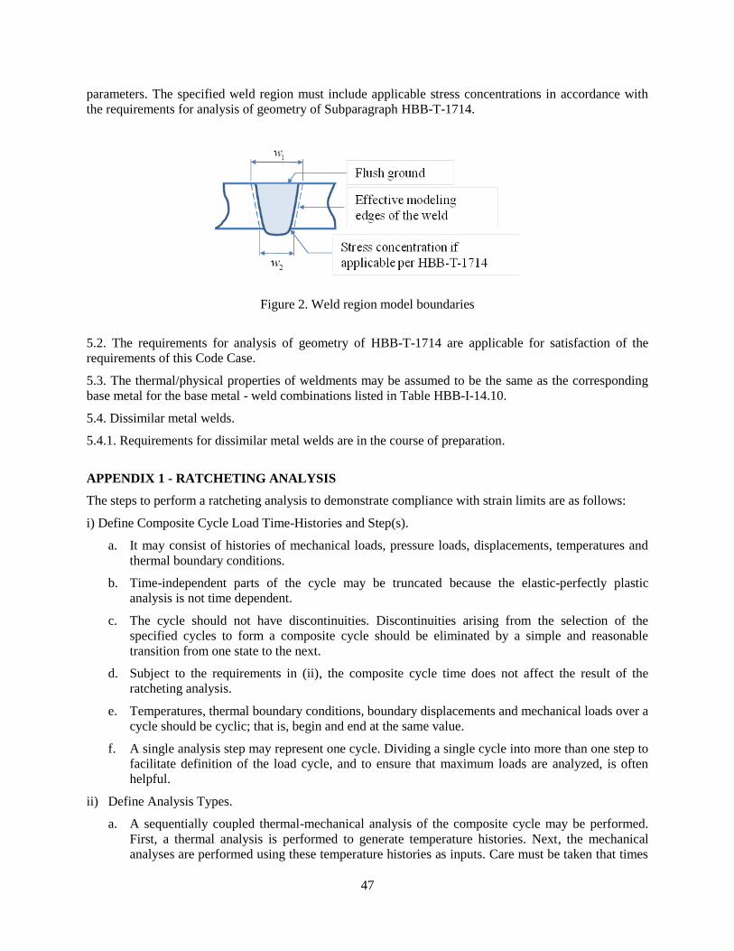
47

parameters. The specified weld region must include applicable stress concentrations in accordance with

the requirements for analysis of geometry of Subparagraph HBB-T-1714.

Figure 2. Weld region model boundaries

5.2. The requirements for analysis of geometry of HBB-T-1714 are applicable for satisfaction of the

requirements of this Code Case.

5.3. The thermal/physical properties of weldments may be assumed to be the same as the corresponding

base metal for the base metal - weld combinations listed in Table HBB-I-14.10.

5.4. Dissimilar metal welds.

5.4.1. Requirements for dissimilar metal welds are in the course of preparation.

APPENDIX 1 - RATCHETING ANALYSIS

The steps to perform a ratcheting analysis to demonstrate compliance with strain limits are as follows:

i) Define Composite Cycle Load Time-Histories and Step(s).

a. It may consist of histories of mechanical loads, pressure loads, displacements, temperatures and

thermal boundary conditions.

b. Time-independent parts of the cycle may be truncated because the elastic-perfectly plastic

analysis is not time dependent.

c. The cycle should not have discontinuities. Discontinuities arising from the selection of the


transition from one state to the next.

d. Subject to the requirements in (ii), the composite cycle time does not affect the result of the

ratcheting analysis.

e. Temperatures, thermal boundary conditions, boundary displacements and mechanical loads over a

cycle should be cyclic; that is, begin and end at the same value.

f. A single analysis step may represent one cycle. Dividing a single cycle into more than one step to

facilitate definition of the load cycle, and to ensure that maximum loads are analyzed, is often

helpful.

ii) Define Analysis Types.

a. A sequentially coupled thermal-mechanical analysis of the composite cycle may be performed.

First, a thermal analysis is performed to generate temperature histories. Next, the mechanical

analyses are performed using these temperature histories as inputs. Care must be taken that times

48

in the mechanical analysis step and in the previous thermal analysis are the same or do not

conflict, depending on the requirements of the analysis software.

b. Alternatively, a coupled thermal-mechanical analysis may be performed. The composite

temperature history to be used in the mechanical analysis should be cyclic, that is the beginning

and end temperature distributions should be the same.

iii) Define Material Properties.

a. For the thermal analyses, density and temperature-dependent specific heat and conductivity will

in general be required.

b. For the mechanical analyses, the temperature-dependent properties required are elastic modulus,

Poisson’s ratio and the mean expansion coefficient. Density may also be required.

c. In addition, the mechanical analyses temperature-dependent yield stress will need to be adjusted

based on the selected pseudo yield stress xTS defined in paragraph 4.2.

iv) Perform Analyses.

a. Perform an elastic-perfectly plastic cyclic mechanical and thermal stress analysis using the

temperature-dependent pseudo yield property defined above. Enough cycles are required to

demonstrate ratcheting or the absence of ratcheting.

b. Care must be taken to ensure that the analysis deals with all the changes within a cycle. Elastic-

plastic analysis routines increase increment size where possible, and may miss a detail in the

loading. A conservative limit to maximum increment size can address this problem, or division of

the cycle into more than one step as in paragraph (i)(f) of this appendix.

v) Detect Ratcheting.

a. Ratcheting is defined as repeated non-cyclic deflections, that is between the beginning and end of

a cycle, a repeated finite displacement change occurs somewhere in the structure.

Detecting ratcheting is most easily done by plotting nodal deflections over time. Cyclic (repeated)

behavior indicates non-ratcheting. History plots of equivalent plastic strains will also identify ratcheting.

49

PART II – BACKGROUND FOR EPP CREEP-FATIGUE CODE CASE

II-1 THEORETICAL BASIS







simplified analysis arises from the use of the “rapid cycle” concept.

Rapid cycles have no creep relaxation during the cycle, but generally have the most advantageous

residual stress system which ensures that deformation rates over the cycle are as low as possible. In terms

of deformation and strain accumulation over time, rapid cycles are more conservative than slow cycles.

Therefore, if creep-fatigue limits can be demonstrated for rapid cycles, slower cycles with relaxation will

also satisfy the creep-fatigue limits. The application of this concept is discussed below in II-1.1 and

illustrated in II-5 and II-Appendix A.

Note that there is no requirement for a high temperature yield property in these arguments. The

restriction on the use of current simplified methods is, essentially, that they are based on yield properties

and the separation of plasticity and creep.

II-1.1 Shakedown Analysis for Cyclic Creep Damage

The proposed creep-fatigue code case uses a conventional (Subsection HB, Subpart B) creep-

fatigue damage summation. The cyclic creep component of damage is defined by an elastic-perfectly

plastic (EPP) shakedown calculation.

Consider a generic high temperature cyclic thermal-mechanical problem, for which thermal and

mechanical cycles have the same period T. There are a number of limiting solutions.

The realistic steady cyclic creep solution (SC) which satisfies ( ) ( )sc sct t T and c

cycle

dt is

kinematically admissible.

The limiting slow cycle or steady state creep solution (SS) for which creep strain rates are

kinematically admissible.

An EPP shakedown solution (SD) is ( ) ( )sd et t where ( )e t is the elastic solution and ρ

is a constant residual stress field. SD solutions are not unique.

The rapid cycle creep solution (RC) ( ) ( )rc e rct t is defined by the residual stress ρrc for

which energy dissipation over a cycle c

cycle

dt is minimized, and c

cycle

dt is kinematically

admissible.

These solutions may be ranked in terms of energy dissipation per cycle as follows (Carter, 2005):

ss sc rc sd (12)

50

The steady cyclic solution and the limiting case of the rapid cycle solution are physically realistic

and achievable, the latter in the limit of short cycle times. The EPP strain limits analysis for the maximum

acceptable design life bears a similar relationship to the RC solution that a reference stress limit analysis

bears to a steady state creep solution.

Because of the point-wise nature of the cyclic creep-fatigue damage EPP calculation, damage and

energy dissipation integrated over the volume are not directly used for prediction of cyclic creep damage.

The example of uniaxial creep-fatigue specimen test is analyzed in II-4, because of its simple

geometry and loading, does have the same connection between the SD and RC solutions that for the more

general problem, only occurs for the strain limits analysis. RC and EPP solutions are illustrated in Fig. II-

16 and Fig. II-17.

As the name implies, the rapid cycle calculation is time-independent. It will be shown that a

shakedown calculation which obtains the maximum point-wise cyclic creep life is effectively making use

of the rapid cycle solution. Any shakedown calculation which obtains an acceptable cyclic creep life is

equal to or more conservative than the rapid cycle solution.

This assertion is checked in detail in calculations for cyclic creep damage in a strain-controlled

creep-fatigue test in II-4.

The use of a time-independent shakedown analysis to bound cyclic creep damage depends on the

similarity between the mathematical descriptions of secondary creep strain rates and average creep

damage rates. Both may be well-characterized by Arrhenius temperature dependencies, and n-power or

hyperbolic sine power laws for stress dependencies.

This means that the creep and rupture behaviors have common features. For a constant load

problem, strain rates generally decrease as the steady state stress distribution is approached in time. If the

creep and damage rates exponents n and n for creep rate and damage rates, are identical, then creep

damage accumulation rate will also be a minimum for the steady state stress distribution. As shown later,

in practice the exponents have to be significantly different for the damage rate not to be a minimum for

cyclic (or steady) conditions.

The intent of the shakedown analysis is to conservatively calculate cyclic creep damage. It may

be summarized as follows. For a defined load cycle:

Define a design rupture time t .

Define a temperature dependent “pseudo” yield stress Sct as the lesser of material minimum yield

stress and stress to cause rupture in time t.

Perform a cyclic elastic-plastic analysis to demonstrate shakedown or otherwise of the

component.

If shakedown occurs, then cyclic creep damage is cD = design life/ t .

The example of a creep-fatigue test analyzed is given in II-4 and II-Appendix A. It shows the

conservatism of the shakedown solution is consistent and reasonable. This covers two aspects.

Average damage rates increase as cycle time is reduced.

The shakedown solution is the realistic limiting case of rapid cycle behavior.

51

II-2. OUTLINE OF EPP CREEP-FATIGUE CODE CASE

A draft of the proposed Creep-Fatigue Code Case is included in II-Appendix B. This code case is

intended as an alternative to the rules in HBB-T-1420 Limits Using Inelastic Analysis, HBB-T-1430

Limits Using Elastic Analysis, and HBB-T-1715 Creep-Fatigue Reduction Factors. There are six parts to

the code case and an appendix. The objective is to comply with the Subsection HB, Subpart B, Appendix

T requirements for creep-fatigue damage evaluation. Namely, that the bounding value of creep damage

fraction combined with the calculated fatigue damage fraction satisfies the allowable creep-fatigue

damage interaction diagram.

Part 1, General Requirements, describes the overall elastic-perfectly plastic shakedown analysis

and provides a general definition of the pseudo yield strength used in this code case. In this code case, the

pseudo yield stress is a temperature dependent, adjusted minimum stress-to-rupture value based on a

selected trial time duration. Also, in this code case, “shakedown” refers to the achievement of cyclic

elastic behavior, without plasticity, throughout the part. The allowable damage due to the combined

effects of the creep damage, Dc, calculated as described in Part 4, and the fatigue damage, Df, calculated

per Part 5, is limited to D as defined by Figure HBB-T-1420-2 Creep-Fatigue Damage Envelope in

Subsection HB, Subpart B

Part 2, Load Definition, identifies the manner in which loads are categorized and grouped for this

application. Code Case procedure requires that a composite cycle be defined which encompasses the

critical features of the individually defined cycles. The reason for this is that the elastic perfectly plastic

methodology used in the code case bounds the long term response independent of the number of applied

cycles. In this respect it is similar to the current simplified rules in Subsection HB, Subpart B.

Two sets of conditions are defined; one set for Service Levels A and B and the other for Service

Levels A and C. A feature of the proposed code case is that, unlike the current version of Subsection HB,

Subpart B, The worst case combinations of Service Level A and B do not need to be combined directly

with Service Level C. The rationale for this is that in accordance with the definition of Service Levels,

shutdown for inspection and repair or replacement is required after a Level C event whereas the reactor

system may resume planned operation after Level A and B events. The number of Level C events is

limited as it is in the lower temperature Division 1, Subsection NB rules, but, unlike the NB rules,

assessment of the high temperature displacement controlled failure modes, strain limits and creep-fatigue,

is required to guard against creep damage not measurable externally which might contribute to restraints

on the remaining life when subjected to subsequent Level A and B conditions.

Part 3, Numerical Model, specifies that the finite element model used in the analysis (The code

case is based on the use of FEA) should accurately represent the component geometry and loading

conditions, transient and steady state, including details such as local stress risers and local thermal

stresses.

Part 4, Calculation of Cyclic Creep Damage, provides the criteria for implementing the code case

evaluation of creep damage based on the use of a pseudo yield stress in a shakedown analysis. The pseudo

yield stress is obtained from the lower of the yield strength adjusted for the aging effects of long time

service at elevated temperature or the minimum stress-to-rupture strength adjusted for the design factor K'

using the values for Elastic Analysis in Table HBB-T-1411-1 of Subsection HB, Subpart B. The time

duration for the stress-to-rupture strength is a trial value equal to or greater than the total design life. The

next step is an elastic-perfectly plastic shakedown analysis using the pseudo yield strength. If shakedown

is achieved, the creep damage, Dc, is the design life divided by the trial time duration. Note that this is a

bounding value for all locations and not the actual creep damage at a specific location. The calculated

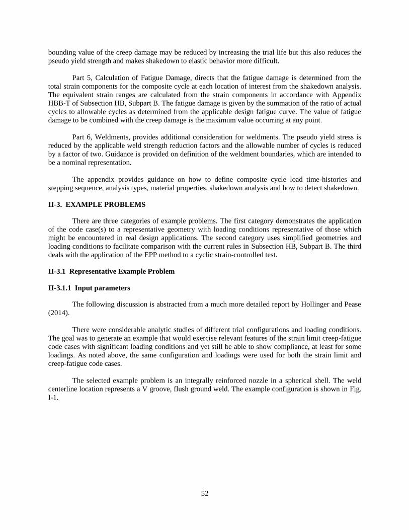
52

bounding value of the creep damage may be reduced by increasing the trial life but this also reduces the

pseudo yield strength and makes shakedown to elastic behavior more difficult.

Part 5, Calculation of Fatigue Damage, directs that the fatigue damage is determined from the

total strain components for the composite cycle at each location of interest from the shakedown analysis.

The equivalent strain ranges are calculated from the strain components in accordance with Appendix

HBB-T of Subsection HB, Subpart B. The fatigue damage is given by the summation of the ratio of actual

cycles to allowable cycles as determined from the applicable design fatigue curve. The value of fatigue

damage to be combined with the creep damage is the maximum value occurring at any point.

Part 6, Weldments, provides additional consideration for weldments. The pseudo yield stress is

reduced by the applicable weld strength reduction factors and the allowable number of cycles is reduced

by a factor of two. Guidance is provided on definition of the weldment boundaries, which are intended to

be a nominal representation.

The appendix provides guidance on how to define composite cycle load time-histories and

stepping sequence, analysis types, material properties, shakedown analysis and how to detect shakedown.

II-3. EXAMPLE PROBLEMS

There are three categories of example problems. The first category demonstrates the application

of the code case(s) to a representative geometry with loading conditions representative of those which

might be encountered in real design applications. The second category uses simplified geometries and

loading conditions to facilitate comparison with the current rules in Subsection HB, Subpart B. The third

deals with the application of the EPP method to a cyclic strain-controlled test.

II-3.1 Representative Example Problem

II-3.1.1 Input parameters

The following discussion is abstracted from a much more detailed report by Hollinger and Pease

(2014).

There were considerable analytic studies of different trial configurations and loading conditions.

The goal was to generate an example that would exercise relevant features of the strain limit creep-fatigue

code cases with significant loading conditions and yet still be able to show compliance, at least for some

loadings. As noted above, the same configuration and loadings were used for both the strain limit and

creep-fatigue code cases.

The selected example problem is an integrally reinforced nozzle in a spherical shell. The weld

centerline location represents a V groove, flush ground weld. The example configuration is shown in Fig.

I-1.

53

Fig. II-1. Representative Example Problem Configuration (dimensions are in inches)

The material selected for the representative example is 316H stainless steel. 316H SS was

selected because it is a material of interest for advanced high temperature reactors and the relevant

material properties are available. There was also an incentive to choose the same material for both the

representative example and the simplified example problems. Since the goal of the simplified examples is

a comparison to the requirements of Subsection HB, Subpart B, it was necessary to also use a material for

which those rules were considered applicable.

The applied loads include thermal and mechanical cyclic loading and a representative seismic

input. Internal pressure and nozzle shear, moment and torsion loads, both sustained and transient, and

thermal transients were specified for Level A, B and C Service Loadings. An overview of these specified

loading histories is shown schematically in Fig. II-2, Fig. I-3 and Fig. II-4, respectively. The detailed

values are tabulated in Hollinger and Pease (2014).

54

Fig. II-2. Service Level A Loads and Load Combinations; loadings versus time

P(t)int.Lev.A

[F(t).Lev.A, V(t).Lev A, M(t).Lev.A, T(t).Lev.A]

t

tA.up

1,100 oFP(t), hin-nozl.Lev.A

675 psig

0 psi; lb, lb-in

70 oF

Max (lb, in-lb)

t A.ss= steady operation

* Ramp rates are calculated in Table xx 70 oF

0 psi; lb, lb-in

tA.down

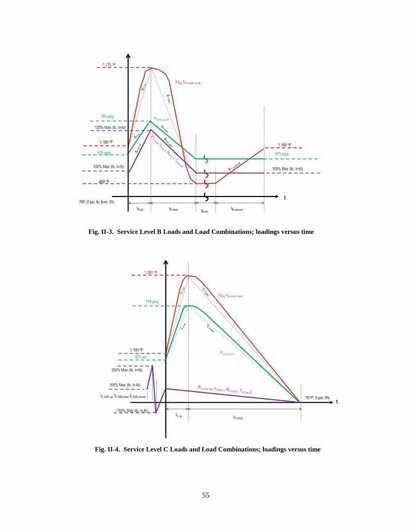
55

Fig. II-3. Service Level B Loads and Load Combinations; loadings versus time

Fig. II-4. Service Level C Loads and Load Combinations; loadings versus time

t

tB.up

1,175 oF

P(t), hin-nozl.Lev.B

750 psig

675 psig

1,100 oF


1,100 oF

675 psig



P(t)int.Lev.B

70F; 0 psi; lb, lb-in; 0%

400 oF

tB.down tB.HStB.recover

tC.up

1,300 oF


775 psig

675 psi

1,100 oF

70 oF; 0 psi; 0%

P(t)int.Lev.C

tC.down

t


-150% Max (lb, in-lb)



56

From these specified loading conditions, the Code Case procedure requires that a composite cycle

be defined which encompasses the critical features of the individually defined cycles. The reason for this

is the elastic-perfectly plastic methodology used in the code case bounds the long term response

independent of the number of applied cycles. In this respect it is similar to the current simplified rules in

Subsection HB, Subpart B. The resultant composite cycle definitions are shown in Fig. I-5 and Fig. I-6 for

Level A and B and Level A and C respectively.

Fig. II-5. Level A and B Composite Cycle

57

Fig. II-6. Level A and C Composite Cycle

Note that two sets of conditions are defined; one set for Service Levels A and B and the other for

Service Levels A and C. A feature of the proposed code case is that, unlike the current version of

Subsection HB, Subpart B, the worst case combinations of Service Level A and B do not need to be

combined directly with Service Level C. The rationale for this is that, in accordance with the definition of

Service Levels, shutdown for inspection and repair or replacement is required after a Level C event

whereas the reactor system may resume planned operation after Level A and B events. The number of

Level C events is limited as it is in the lower temperature Division 1, Subsection NB rules, but, unlike the

NB rules, assessment of the high temperature displacement controlled failure modes, strain limits and

creep-fatigue, is required to guard against creep damage not measurable externally which might

contribute to restraints on the remaining life when subjected to subsequent Level A and B conditions.

II-3.1.2. FEA model and material properties

The FEA models are shown in Fig. I-7, without the weld zone, Fig. I-8, with the weld zone, from

Hollinger and Pease (2014). The model consists of 8-node linear brick elements with full integration for

stress analysis and 8-node linear heat transfer brick elements for that analysis. The same mesh is used for

both the stress and heat transfer element types. The supporting mesh density study is shown in Appendix

A of Hollinger and Pease (2014).

tC.up

1,300 oF


775 psig

675 psi

1,100 oF

70 oF; 0 psi; 0%

P(t)int.Lev.C

tC.down

t


-150

% M

ax (l

b, in

-lb)



0 psi; 0%

70 oF

tA.UP tA.SS

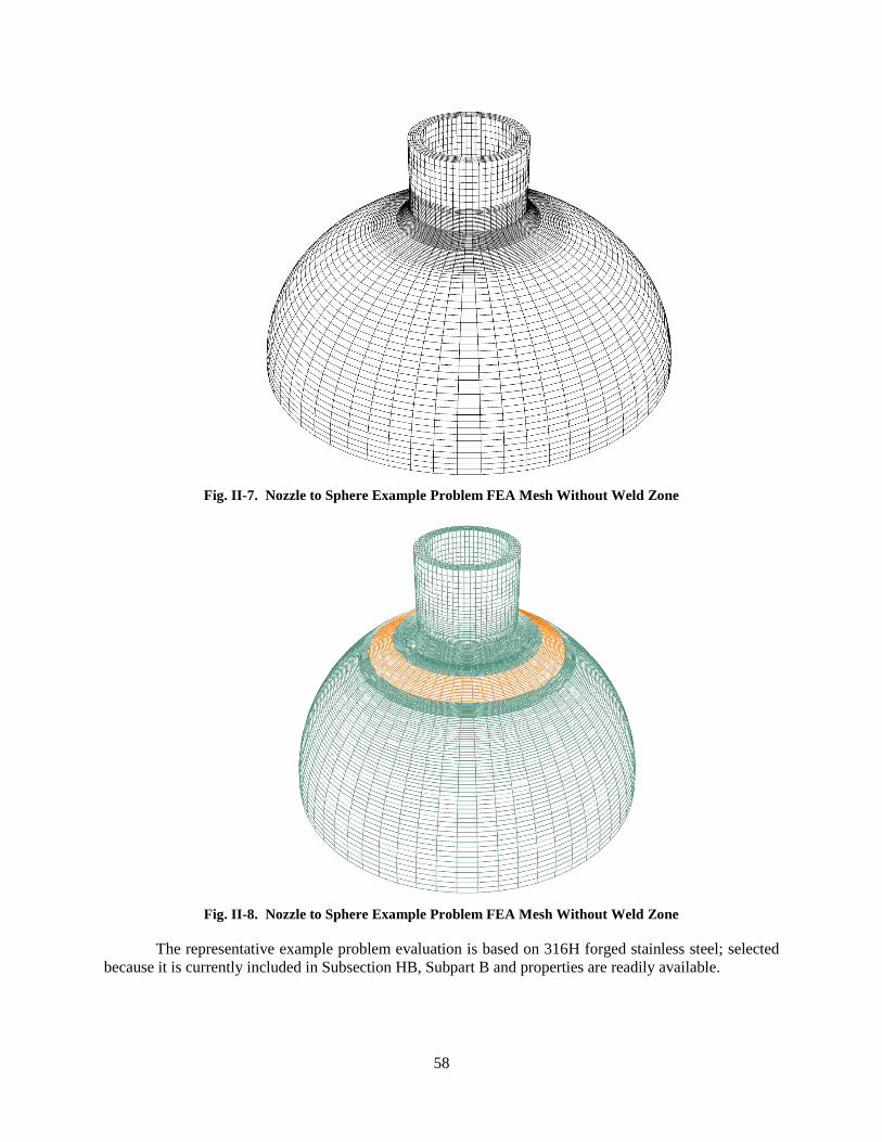
58

Fig. II-7. Nozzle to Sphere Example Problem FEA Mesh Without Weld Zone

Fig. II-8. Nozzle to Sphere Example Problem FEA Mesh Without Weld Zone

The representative example problem evaluation is based on 316H forged stainless steel; selected

because it is currently included in Subsection HB, Subpart B and properties are readily available.

59

II-3.1.3 Methodology

Two types of analyses are run for each set of composite cycles. A transient heat transfer analysis

is performed to establish the temperature field in the vessel throughout the composite cycle. A

representative FEA plot is shown below, Fig. I- 9, illustrating the temperature distribution at the end of

the Service Level B peak up ramp to 1175 oF.

Fig. II-9. Level B Peak Up (1175 oF)

Stress analyses are performed with the time dependent temperature field results from the heat

transfer analysis to obtain the stresses and strains in the vessel due to both mechanical loads and thermal.

Note: Each cycle of a stress analysis using a "pseudo yield stress" has no direct correlation to the number

of design or fatigue cycles and is hence defined as a "pseudo-cycle". Each composite cycle is broken up

into discrete steps and when necessary limits to maximum time increments are applied to ensure that the

analysis deals with all the changes within a cycle. The step names and durations are plotted with the time

history amplitudes in Fig. I-10 and Fig. I-11.

60

Fig. II-10. Level A&B Composite Cycle Steps

Fig. II-11. Level A & C Composite Cycle Steps

0.0

0.2

0.4

0.6

0.8

1.0

1.2

1.4

0

200

400

600

800

1000

1200

1400

Leve

l A: R

amp

Up

Leve

l A: S

tead

y Sta

te 1

Leve

l B: R

amp

Up

Leve

l B: P

eak U

p

(10

sec m

ax in

crem

ents)

Leve

l B: P

eak D

own

(10

sec m

ax in

crem

ents)

Leve

l B: R

amp

Down

1

Leve

l B: R

amp

Down

2

Leve

l B: R

amp

Down

3

Leve

l B: R

amp

Down

4

Leve

l B: H

old S

tate

Leve

l B: R

ecov

er

Leve

l A: S

tead

y Sta

te 2

Leve

l A: R

amp

Down

Shutd

own:

Ste

ady S

tate

Mec

han

ical

Lo

ad F

acto

r

Tem

per

atu

re, °

F

Pre

ssu

re, p

si


-2.0

-1.5

-1.0

-0.5

0.0

0.5

1.0

1.5

2.0

2.5

0

200

400

600

800

1000

1200

1400

Leve

l A: R

amp

Up

Leve

l A: S

tead

y Sta

te 1

Leve

l C: S

SE Up

Leve

l C: S

SE Dow

n

Leve

l C: S

SE Rec

over

Leve

l C: R

amp

Up

Leve

l C: P

eak U

p

(10

sec m

ax in

crem

ents)

Leve

l C: P

eak D

own

(10

sec m

ax in

crem

ents)

Leve

l C: R

amp

Down

1

Leve

l C: R

amp

Down

2

Leve

l C: R

amp

Down

3

Shutd

own:

Ste

ady S

tate

Mec

han

ical

Lo

ad F

acto

r

Tem

per

atu

re, °

F

Pre

ssu

re, p

si


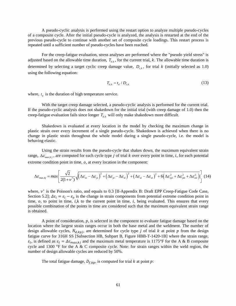
61

A pseudo-cyclic analysis is performed using the restart option to analyze multiple pseudo-cycles

of a composite cycle. After the initial pseudo-cycle is analyzed, the analysis is restarted at the end of the

previous pseudo-cycle to continue with another set of composite cycle loadings. This restart process is

repeated until a sufficient number of pseudo-cycles have been reached.

For the creep-fatigue evaluation, stress analyses are performed where the "pseudo yield stress" is

adjusted based on the allowable time duration, ,d kT , for the current trial, 𝑘. The allowable time duration is

determined by selecting a target cyclic creep damage value, ,c kD , for trial 𝑘 (initially selected as 1.0)

using the following equation:

, ,/d k d c kT t D (13)

where, dt is the duration of high temperature service.

With the target creep damage selected, a pseudo-cyclic analysis is performed for the current trial.

If the pseudo-cyclic analysis does not shakedown for the initial trial (with creep damage of 1.0) then the

creep-fatigue evaluation fails since longer ,d kT will only make shakedown more difficult.

Shakedown is evaluated at every location in the model by checking the maximum change in

plastic strain over every increment of a single pseudo-cycle. Shakedown is achieved when there is no

change in plastic strain throughout the whole model during a single pseudo-cycle, i.e. the model is

behaving elastic.

Using the strain results from the pseudo-cycle that shakes down, the maximum equivalent strain

range, ,max k j , are computed for each cycle type 𝑗 of trial 𝑘 over every point in time, 𝑖, for each potential

extreme condition point in time, 𝑜, at every location in the component:

2 2 2 2 2 2

, *

2 6

2(1 )max kj xi yi yi zi zi xi xyi yzi zximax

(14)

where, 𝜈∗ is the Poisson's ratio, and equals to 0.3 [II-Appendix B: Draft EPP Creep-Fatigue Code Case,

Section 5.2]; 𝛥𝜀𝑖 = 𝜀𝑖 − 𝜀𝑜 is the change in strain components from potential extreme condition point in

time, 𝑜, to point in time, 𝑖,k to the current point in time, 𝑖, being evaluated. This ensures that every

possible combination of the points in time are considered such that the maximum equivalent strain range

is obtained.

A point of consideration, 𝑝, is selected in the component to evaluate fatigue damage based on the

location where the largest strain ranges occur in both the base metal and the weldment. The number of

design allowable cycles, 𝑁𝑑,𝑘𝑝𝑗, are determined for cycle type 𝑗 of trial 𝑘 at point 𝑝 from the design

fatigue curve for 316H SS [Subsection HB, Subpart B, Figure HBB-T-1420-1B] where the strain range,

𝜀𝑡, is defined as 𝜀𝑡 = 𝛥𝜀𝑚𝑎𝑥,𝑘𝑗 and the maximum metal temperature is 1175°F for the A & B composite

cycle and 1300 °F for the A & C composite cycle. Note: for strain ranges within the weld region, the

number of design allowable cycles are reduced by 50%.

The total fatigue damage, 𝐷𝑓,𝑘𝑝, is computed for trial 𝑘 at point 𝑝:

62

,

,

j

f kp

j d kpj

nD

N (15)

where, 𝑛𝑗 is the number of applied cycles for cycle type 𝑗.

If the total fatigue damage is not less than 1.0 then the creep-fatigue evaluation has failed.

The allowable creep-fatigue damage, 𝐷𝑘𝑝, is determined for trial 𝑘 at point 𝑝:

11

11

icf ,kp

if

kp f ,kp

icf ,kp

if

D D

DD D max

DD

D

(16)

where, (𝐷𝑖𝑓 , 𝐷𝑖𝑐) is the creep-fatigue damage envelope intersection parameters [Subsection HB, Subpart

B, Figure HBB-T-1420-2], and equals to (0.3, 0.3) for 316H stainless steel

The total creep-fatigue damage for trial 𝑘 is computed and compared to the allowable damage for

trial 𝑘 at point 𝑝:

, ,f kp c k kpD D D (17)

Note: The creep damage used in this equation is not necessarily the creep damage at a specific

point, but is the “maximum cyclic creep damage over the structure” as specified in Section 4.4 of the

Creep Fatigue Code Case.

If the total creep-fatigue damage exceeds the allowable damage then a reduced target creep

damage, 𝐷𝑐,𝑘+1, is selected for the next trial, 𝑘 + 1, based on the following equation:

, 1 ,c k kp f kpD D D (18)

The above process is repeated until either the creep-fatigue evaluation passes the criterion of Eqn.

(17) or fails due to excessive creep or fatigue damage or both.

II-3.1.4 Results

Results were generated for two FEA models, base metal only and base metal plus weldment. The

results are slightly different due to affect the lower pseudo yield strength of the weldment (reduced by the

weld strength reduction factor) has on the surrounding base metal. The following is based on the

weldment model with relevant differences noted.

Level A & B composite cycle evaluation

The controlling base metal location for both models is at the outer surface of the shell-to-nozzle

transition, rotated approximately 45° from where nozzle bending due to the nozzle end shear load

produces maximum strains. The Level A & B cycle type maximum equivalent strain range at this location

for both the base metal only model and the model with the weldment is 0.110%. However, for the Level B

63

cycle type they are slightly different, 0.076% and 0.077% respectively. The controlling weldment location

is on the inside surface of the shell on the outermost weld-base metal interface. The maximum equivalent

strain range at this location from both models is 0.083% for the Level B cycle type and 0.037% for the

Level A cycle type.

The weldment model Level A & B Composite Cycle analysis with a target creep damage of 0.95

passes after 3 pseudo-cycles. The base metal only model passes with a target creep damage of 0.90, also

after 3 pseudo cycles. For the weldment model, the total creep-fatigue damage is 0.954 and the allowable

creep-fatigue damage is 0.995, which is sufficiently greater than the calculated value. This places the

creep-fatigue damage within the HBB-T-1420-2 creep-fatigue interaction envelope, thus meeting the

criteria for creep-fatigue interaction for the base metal. For the base metal only model, the corresponding

total and allowable damages are 0.904 and 0.995 respectively.

In the weld region, the corresponding values of total damage and allowable damage are 0.958 and

0.988 respectively.

Level A & C composite cycle evaluation

The base metal only creep-fatigue evaluation for the Level A & C Composite Cycle with a target

creep damage of 1.0 does not pass after 20 pseudo-cycles. The change in plastic strain after each pseudo-

cycle is 0.28% indicating that stable ratcheting continues and shakedown does not occur. Further

reduction of the target creep damage will only produce weaker pseudo-yield stresses, resulting in even

more severe ratcheting.

Since the base metal only evaluation did not pass for the Level A & C Composite Cycle the

weldment model evaluation will not pass either.

II-3.2 Creep-Fatigue Code Case to Subsection HB, Subpart B Comparison

The overall goal of this phase is to assess the design margins in the EPP methodology. This is

accomplished through the use of simplified example problem solutions which include comparison to

current Subsection HB, Subpart B procedures. Simplified examples are used to avoid the complexities of

Subsection HB, Subpart B simplified procedures, particularly when applied to representative geometries

and loading.

II-3.2.1 Geometry and material

Case 1. Plain tube with r/t = 4.5, outer diameter (OD) = 15in, Material: 316H stainless steel.

Case 2. Plain tube with r/t = 3.5, OD=16in, Material: 316H stainless steel.

Case 3. Case 1 connected to Case 2, with a 3:1 external taper in wall thickness.

II-3.2.2 Level A/B service loadings

These calculations will be based on a design pressure of 1.3 ksi in both tubes, and a temperature

cycle defined by a uniform 1075 oF to the temperature distributions defined below.

For tube #1, consider steady state metal temperatures defined by 1200 oF in the bore, and 1075

oF

on the OD. Using the formula for thermal stress in a tube with through-wall heat flux in Pitts and Sissom

(1998), the radial steady state heat flux for these temperatures is 105 BTU/in/in/hour. The steady state

bore temperature in tube #2 for this heat flux and the 1075 oF tube OD temperature is 1235

oF. A heat flux

64

cycle from zero to 105 BTU/in/in/hour is used in the following steady state thermal-mechanical

calculations.

Thermal-mechanical properties at 1100 oF are given in Table II-1. Thermal and mechanical

elastic stresses are obtained from thick-walled pipe formulas in Roark and Young (1989).

Table II-1. Thermo-mechanical properties of TP316 at 1100

oF

Spec. Heat

BTU/(lb⋅ oF)

Conductivity

BTU/(hr⋅in⋅°F)

Exp. Coefficient

in/in/oF

Young's Modulus

ksi

143.14 1.1055 1.029E-05 21928

Fig. II-12 shows combined pressure stress and thermal stress contours, and the corresponding

linearized stress components. It is seen that the stress contour plot and the linearized plot agree, and the

second order mesh density is shown to indicate that this agreement is not due to a coarse mesh.

Fig. II-12. Hoop Pressure Plus Thermal Stress. Maximum Value of both Stresses is 44 ksi. Second Order

Finite Element Mesh Indicated.

65

The equivalence between the maximum stress for these calculations shows that in this case there is no

need for a stress concentration factor K > 1 in the creep-fatigue calculation.

II-3.2.3 HBB-T-1430 limits using elastic analysis

The HBB-T-1413 calculation of strain range is based on full strain components without

distinction between elastic-plastic and thermal components. In these calculations K = 1 for a non-welded

component with stresses as shown in Fig. II-12. The HBB-T-1433 stress and creep damage calculations

for a pipe subject to through wall thermal stress cycles proceeds as follows:

Calculate bore and OD temperatures.

Calculate axial and circumferential thermal stress and strain.

Calculate bore radial strain.

HBB-T-1432 (a) – (c). Calculate (HBB –T-1413) max modequiv ( 1)nK K .

HBB-T-1432 (g). Calculation of c per cycle from stress =1.25 c at 1235 0F, where

c yZS .

HBB-T-1432 (h). Total strain range modt c .

HBB-T-1433 (a). HBB-T-1324. Since 3 /t mS E relaxation damage calculation per cycle is

required.

HBB-T-1433 Step 4. Calculate initial thermal stress from zero time isochronous data and bore

temperature.

HBB-T-1433 Step 5 (b). Calculate stress relaxation using isochronous data at 1235 oF, limited by

1.25 core stressLBS . This limit is reached after 18.5 hours of relaxation. No further

(multiaxial) correction is required in Step 5 (b).

Load controlled stress intensities (primary elastic plus bending value assumed) = 5ksi and are

constant during the cycle. This value is always less than the relaxed stress, and does not affect the

damage calculation.

Calculate fatigue damage based on t .

Calculate creep-fatigue damage with creep-fatigue interaction from Fig. HBB-T-1420-2.

Tube #2 was assessed for creep-fatigue damage. The results for the thermal stresses and strains

for Tube #2 is shown in Table II-2.

Table II-2. Thermo-mechanical bore strain range: Tube 2 (HBB-T-1413)

Bore principal stresses ksi Temp, oF Strains

Hoop Axial Radial Hoop Axial Radial

4.64 1.67 -1.3 1075 0.0113 0.0112 0.0110

-23.18 -26.15 -1.3 1235 0.0119 0.012 0.0134

4.64 1.67 -1.3 1075 0.0113 0.0112 0.011 Effective

strain range

Strain

ranges

0.0007 0.0007 0.00243 1.30E-03

66

Table II-3. Tube 2 strain range per cycle

Cycle time c per cycle t

100 3.481E-03 4.768E-03

300 7.421E-03 8.527E-03

Table II-4 shows relaxation and creep damage for the strain in Table II-2. The results are limited

by the (1.25 × 𝑐𝑜𝑟𝑒 𝑠𝑡𝑟𝑒𝑠𝑠) relaxation stress limit and the maximum cycle time of 300 hours.

Table II-4. Hot relaxation and creep damage calculation: Tube 2

Relaxation Creep damage Strain

HBB-T-1433 (b) K' = 0.9 1.2901E-03

stress: Figure HBB-T-1800-B-9 SLB = 12.42 ksi

max stress rupture time with

stress/0.9 hours Damage

19.23 1.850E+02 0 0.00

16.86 4.093E+02 1 0.01

13.34 1.629E+03 10 0.03

12.42 2.460E+03 18.5 0.03

12.42 2.460E+03 100 0.07

12.42 2.460E+03 300 0.15

Table II-5 shows the Subsection HB, Subpart B fatigue and relaxation creep damage calculation

results, and the creep-fatigue life for the 16” OD tube, for 100 hour and 300 hour cycles respectively. This

calculation assumes repeated re-setting and stress relaxation for each cycle as per the requirements of

HBB-T-1432. Table II-5 indicates a maximum acceptable life of 1,430 hours for 100 and 300 hour cycles.

Table II-5. Tube 2 creep-fatigue life calculation HBB-T-1411

Hours cycles cycle time t fatigue life

1290 12.9 100.0 4.768E-03 324

1650 5.5 300.0 8.527E-03 75

fatigue

damage

creep damage cd1 cf1 Cfdam

3.99E-02 0.903 0.3 0.3 1.00

7.34E-02 0.825 0.3 0.3 1.00

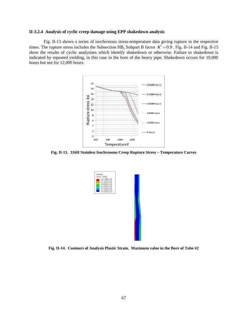
67

II-3.2.4 Analysis of cyclic creep damage using EPP shakedown analysis

Fig. II-13 shows a series of isochronous stress-temperature data giving rupture in the respective

times. The rupture stress includes the Subsection HB, Subpart B factor 0.9 K . Fig. II-14 and Fig. II-15

show the results of cyclic analysises which identify shakedown or otherwise. Failure to shakedown is

indicated by repeated yielding, in this case in the bore of the heavy pipe. Shakedown occurs for 10,000

hours but not for 12,000 hours.

Fig. II-13. 316H Stainless Isochronous Creep Rupture Stress – Temperature Curves

Fig. II-14. Contours of Analysis Plastic Strain. Maximum value in the Bore of Tube #2

68

Fig. II-15. Plots of Cyclic Plastic Strain from Tube Bore. Shakedown Obtained for 10,000 Hours Rupture

Life, Failure to Shakedown for 12,000 Hours Rupture Life

Table II-6 gives the creep-fatigue calculation with a cyclic creep-fatigue life of 10,000 hours for

two cases with different cycle times. Because fatigue damage is insignificant, the results for the two cases

are the same.

Table II-6. Tube 2 creep-fatigue life calculation EPP shakedown analysis

Hours cycles cycle time

(h) t fatigue life

10,000 100.0 100.0 1.290E-03 1.00E+05

10,000 33.3 300.0 1.290E-03 1.00E+05

fatigue

damage

creep damage cd1 cf1 Cfdam

1.00E-03 1.00 0.3 0.3 1.00

3.33E-04 1.00 0.3 0.3 1.00

II-3.2.5 Summary

Creep-fatigue damage was evaluated to compare the results from the current Subsection HB,

Subpart B procedures to the results from the proposed creep-fatigue code case using elastic-perfectly

plastic methods. The evaluation was done using a relatively thick wall cylinder, 16 inches OD with 2

inches wall thickness. The steady state condition is an inner wall temperature of 1235 oF and an outer wall

temperature of 1075 oF. The heat flux is periodically cycled to zero while maintaining the inner wall

temperature constant such that the outer wall temperature equals the inner wall temperature. The material

is 316H stainless steel. The estimated allowable life from the current Subsection HB, Subpart B procedure

is 1430 hours as compared to an estimated life of approximately 10,000 hours using the proposed EPP

creep-fatigue code case.

69

II-4. BOUNDING THEORY EXAMPLE CALCULATION

II-4.1 Analysis of Strain Controlled Creep-Fatigue Test Specimen

In this section, the EPP shakedown analysis is applied to the case of a strain-controlled creep-

fatigue test. The II-Appendix A provides further details of calculations for stress and creep damage for a

strain- controlled cyclic test.

Consider an example with ASME Section III, Division 5 Subsection HB, Subpart B Data for

316H stainless steel at 1400 oF. The test is characterized by a strain cycle at temperature T.

For stress 2 5 12. ksi , creep and damage rates are:

,nc

nc

dk

dt

dDk

dt

where constants k, k’, n, n’ are shown in Table II-7.

Table II-7. Creep and damage constants for 316H stainless steel at 1400

oF. Units: ksi,

oF, hours

strain rate (n,k) damage rate (n', k')

n, n' 5.192 4.369

k, k' 2.1992E-09 5.2083E-08

The solutions of interest are:

Assuming the test strain range shakes down, that is 2 ,yE the EPP solution, which has

equal and opposite stresses, is:

1 / 2E

2 1

Steady cyclic creep solution ( )t satisfied the following equations, derived in II-Appendix A.

1 1( ) (0)

1 1

n ntEkt

n n

(19)

1

1 1( ) (0) ( 1) n nt n Ekt (20)

/2

1

0( )

( 1 )

n n

c

kD t

kE n n

(21)

The ratio of the cyclic creep and EPP solution damage calculations is:

70

/21

0

/2 '1

0

( )1

1 ' ( ) [ (0) ( / 2)] / 2

n n

nn

tn

n n t

(22)

Examples of relatively rapid and slow cycles for strain range = 0.001 at 1400 oF are shown in Fig.

II-16 and Fig. II-17. These figures show cyclic relaxation stress histories, the constant EPP reference

stresses, and creep damage calculated from the creep and EPP stress histories, respectively. Fig. II-16

represents a cycle time of 1 hour, and Fig. II-17 represents a cycle time of 10 hours. The relaxation stress

history is calculated from Eqns. (19) and (20), and the creep damage from Eqn. (21).

Fig. II-16. Stress and damage histories for 1 hour cycle time

These figures show the conservatism of the EPP creep damage calculation compared with the

relaxation creep damage calculation. The conservatism increases for longer cycle times, as shown in Fig.

II-17 which is calculated from Eqn. (22).

Fig. II-18 shows the ratio of the relaxation creep damage to the EPP design value, /c eppD D . For

realistic values of the creep strain rate and creep damage rate exponents n and n’ as in Table 2.6.1,

/ 1c eppD D . Values of the creep damage exponent ' 2n n are required to give / 1c eppD D . The ratio

/c eppD D always decreases as hold time increases. Alternatively, as 0, / 1c eppD D .

71

Fig. II-17. Stress and damage histories for 10 hour cycle time

Fig. II-18. Effect of Cycle Time on EPP Conservatism

II-4.2 Process Flow Procedure for Bounding Creep Damage in Creep-Fatigue Specimen

This procedure illustrates the bounding characteristics of the EPP creep-fatigue evaluation

without resorting to theoretical arguments. Thus demonstrating the validity of the basic theory as applied

to this specific simplified example.

The example problem, Fig. II-19 is the same as used in II-3.3.1 and II-Appendix A. It is a uniform bar

with a cyclic displacement controlled load. For evaluating creep damage due to the realistic steady

cyclic solution, the material behavior is assumed to be elastic-creep. For illustration only, it will be

assumed that fatigue damage is negligible. The trial life, t, is the longest life for which the applied

displacement amplitude, δ, causes the uniform bar to just shake down with a time dependent pseudo

yield strength Sct.

72

Fig. II-19. Applied Loading

The trial pseudo yield strength is based on the creep-rupture strength as a function of time and

temperature. (Note, the design factor, K’, is omitted from this example for clarity.)

Iterate the trial time and corresponding pseudo yield stress until the elastic-perfectly plastic solution

reaches the longest time for which elastic shakedown is achieved. (Note, for the code case evaluation,

it will be conservative to use a trial time that shakes down but may not be the longest achievable).

This is the EPP solution as shown in Fig. II-20, where 0, 1, … 5 are the corresponding loading points

in the time independent composite cycle, , and ctS is the pseudo yield strength.

Fig. II-20. EPP Solution

Since the EPP loading sequence is time independent it also represents the bounding creep damage due

to n cycles with period τ where n τ = t, the trial time used to define Sct. See Fig. II-20 repeated below

and Fig. II-21.

2δ

Time0

(1) (2)

(3) (4)

(5)

Sct

-Sct

73

Fig. II-21. EPP Solution with Period t

However, Fig. II-22 is equivalent to the rapid cycle solution (RC) for this problem and it has been

shown in II-3.3.1 and II-Appendix A that the rapid cycle solution for this example bounds the actual

steady cyclic creep solution for the same loading and period. See Fig. II-21 repeated and Fig. II-22

below.

Fig. II-22. Bounding solution Compared to Analytical Solution

Time

Sct

τ

Time

t

n cycles

-Sct

Fig. 20

t

Sct

-Sct

Fig. 21

Time

Steady Cyclic (SC) Solution

Rapid Cyclic (RC) => EPP

τ

Time

Sct

τ

-Sct -Sct

Sct

74

II-5 EXPERIMENTAL RESULTS COMPARISON

II-5.1 Experimental Procedure

The experimental procedure is based on modified creep-fatigue test specimens that incorporate

elastic follow-up characterization of stress and strain redistribution due to creep. Suitably sized specimens

based on elastic-follow-up concepts are cycled to failure and the data generated used to evaluate the

applicability of the EPP methodology. Elastic follow-up can cause larger strains in a structure with

displacement controlled loading than would be predicted using an elastic analysis. These strain

concentrations may result when structural parts of different flexibility are connected in series and loaded

by an applied displacement and the flexible parts are highly stressed. This approach to creep-fatigue

testing is referred to as the Simplified Model Test (SMT) approach as proposed by Jetter (1998).

The basic concept of the SMT methodology is shown in Fig. II-23. The component design is

represented by a stepped cylinder with a stress concentration at the shoulder fillet radius. The component

has a global elastic follow-up, , which is due to the interaction between the two cylindrical sections,

and a local follow-up, , which is due to the local stress concentration. Generally, is the ratio of the

elastic follow-up strain to the elastically calculated strain. If the thick cylinder is displaced radially inward

a fixed amount, , there will be a maximum strain at the stress concentration. Although the actual

strain may be higher, the relevant parameter in this approach is the maximum elastically calculated strain

in the component, . The effects of plasticity, creep and strain redistribution are accounted for in

the SMT simulation.

(a) Shell structure with

stress concentration and

elastic follow-up

(b) Design curve (c) Hold time creep-fatigue test with

elastic follow-up

Fig. II-23. SMT methodology

In order to be effective, the SMT specimen must be sized to provide a stress-strain hysteresis loop

under cyclic loading which envelopes the hysteresis loop of components of interest.

nq

Lq q

comp

, E comp

test

,E test

testq

Ela

stic

all

y C

alc

ula

ted

Str

ain

Ra

ng

e

N Allowable Cycles

nq

comp

Lq

, E comp

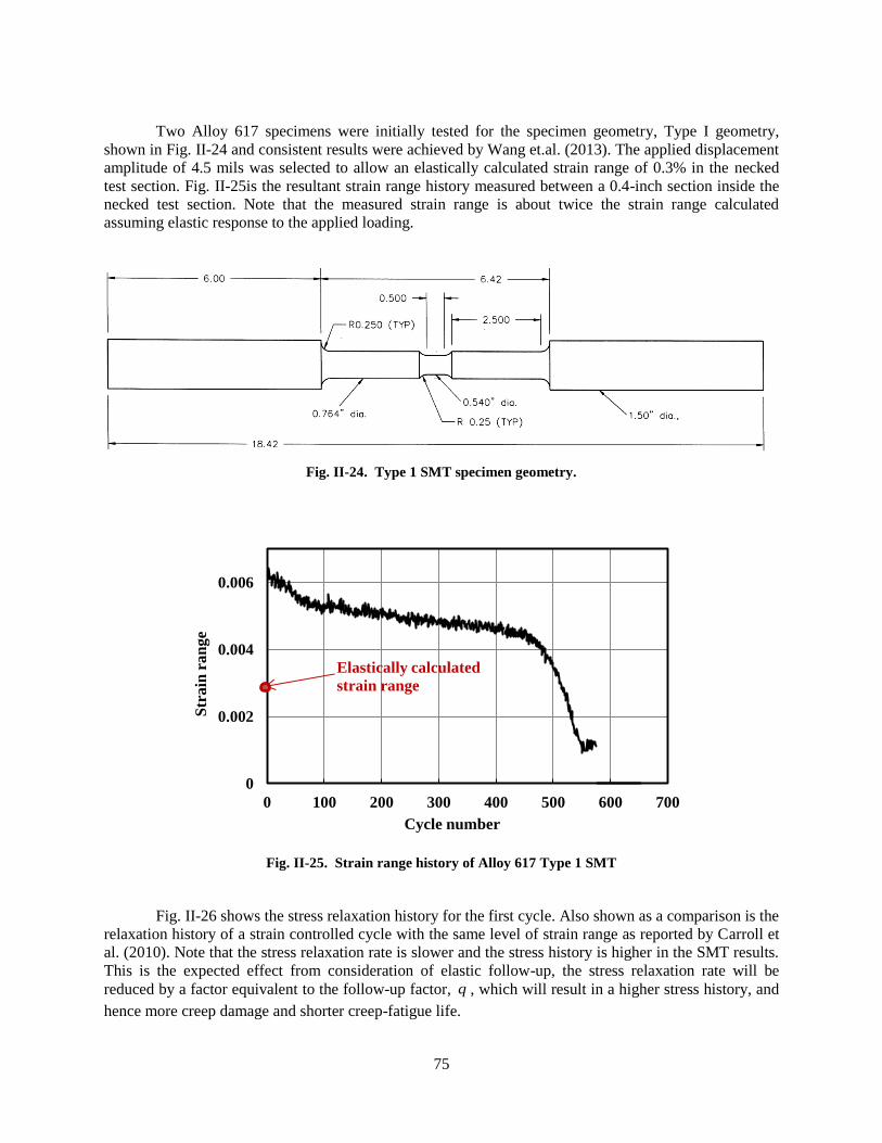
75

Two Alloy 617 specimens were initially tested for the specimen geometry, Type I geometry,

shown in Fig. II-24 and consistent results were achieved by Wang et.al. (2013). The applied displacement

amplitude of 4.5 mils was selected to allow an elastically calculated strain range of 0.3% in the necked

test section. Fig. II-25is the resultant strain range history measured between a 0.4-inch section inside the

necked test section. Note that the measured strain range is about twice the strain range calculated

assuming elastic response to the applied loading.

Fig. II-24. Type 1 SMT specimen geometry.

Fig. II-25. Strain range history of Alloy 617 Type 1 SMT

Fig. II-26 shows the stress relaxation history for the first cycle. Also shown as a comparison is the

relaxation history of a strain controlled cycle with the same level of strain range as reported by Carroll et

al. (2010). Note that the stress relaxation rate is slower and the stress history is higher in the SMT results.

This is the expected effect from consideration of elastic follow-up, the stress relaxation rate will be

reduced by a factor equivalent to the follow-up factor, , which will result in a higher stress history, and

hence more creep damage and shorter creep-fatigue life.

0

0.002

0.004

0.006

0 100 200 300 400 500 600 700

Str

ain

ra

ng

e

Cycle number

Elastically calculated

strain range

q

76

Fig. II-26. Stress relaxation during the hold period for Type 1 SMT necked test

section and standard creep-fatigue specimen, Carroll et al. (2010).

II-5.2 Elastic-Perfectly Plastic Simulation on Alloy 617 Creep-Fatigue

Creep-fatigue tests have been conducted on Alloy 617 standard ASTM creep-fatigue specimens at

850 o

C and 950 oC, and on key-feature test articles of Alloy 617 at 950

oC. The key feature test articles,

the so-called Simplified Model Test (SMT) geometries, were developed to mock up the effects of elastic

follow-up in reactor pressure boundary components. These data provide an opportunity to assess the

conservatism of the EPP creep-fatigue procedure developed for very high temperature applications.

Young’s modulus, E , shear modulus, G , yield strength, yS , minimum rupture strength,

rS , and

pseudo yield stress are material parameters required in the EPP creep-fatigue evaluation procedure. The

temperature dependence of E , G and yS for Alloy 617, given in the units of MPa, are given as

6 3 3 2 37.57834280 3.06384( 586 52.8928996 227.043102) 10 10 10k k k kE T T T T (23)

6 3 3 2 36.14747367 5.87486( 911 25.2278723 88.4508513) 10 10 10k k k kG T T T T (24)

9 3 6 2

3

2.78261712 10 6.45428719 10( ) 240

4.96338300 10 1.98846231

k k

y k

k

T TS T

T

(25)

where kT is the absolute temperature in kelvin. The data for

yS were based on testing to high temperature

ASTM tensile testing standard.

The correlation for the minimum rupture strength in the units of MPa was given by Eno et al.

(2008) as:

0

10

20

30

0 100 200 300 400 500 600

Aver

age

stre

ss, k

si

Hold time, s

SMT, neck region, cycle 1

Standard creep fatigue, cycle 1

77

1/ 1/expm m

r r

k

QS A t

mRT

(26)

where rt is the rupture time in hours and

0 1 2 3

0 1 2 3

exp , , /

20.07 0.356 10 , 37531 10 , 1.20, 7568

8.314472151.645,

kA Q R m T

z n n

z R

(27)

The pseudo yield stress is given as:

y rpseudo yield stress lesser of S ,K S (28)

where K is a design factor that has a value of 0.9 .

The EPP creep-fatigue code case specifies the use of a pseudo yield stress corresponding to a trial

time dT that is greater than or equal to the design time

designt for the EPP finite element analysis. A trial

time of d designT t sets the critical condition for assessing if shakedown to elastic action would take place.

That is, if an EPP finite element analysis could not demonstrate shakedown to elastic action when

d designT t is used to set the pseudo yield stress, shakedown to elastic action would not take place for any

other selected time d designT t to set the pseudo yield stress.

II-5.3 Standard Alloy 617 Creep-Fatigue Tests

The geometry of the standard creep-fatigue test specimen, with a gage diameter of 7.49 mm,

conforms to the ASTM E2714 standard. The tests were conducted under uniform temperature and strain

controlled conditions. Loading and unloading within a creep-fatigue cycle were carried out at a prescribed

strain rate, and a strain hold was imposed at maximum tensile strain within the cycle for a specified

period. The straining cycles were fully reversed cycles.

For the consideration of these set of tests with respective to the EPP creep-fatigue procedure, the

design time is taken to be the life time of the creep-fatigue test specimen, and hence it is calculated as

time per cycle multiplied by the observed/measured cycles to failure. The creep-fatigue test conditions

and the test data, which were provided by L. Carroll of the Idaho National Laboratory, are shown in Table

II-8.

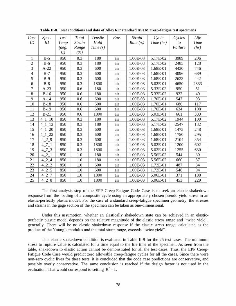
78

Table II-8. Test conditions and data of Alloy 617 standard ASTM creep-fatigue test specimens

Case

ID

Spec.

ID

Test

Temp

(deg.

C)

Total

Strain

Range

(%)

Tensile

Hold

Time (s)

Env. Strain

Rate (/s)

Cycle

Time (hr)

Cycles

to

Failure

Life

Time

(hr)

1 B-5 950 0.3 180 air 1.00E-03 5.17E-02 3989 206

2 B-6 950 0.3 180 air 1.00E-03 5.17E-02 2485 128

3 A-22 950 0.3 600 air 1.00E-03 1.68E-01 4430 746

4 B-7 950 0.3 600 air 1.00E-03 1.68E-01 4096 689

5 B-9 950 0.3 600 air 1.00E-03 1.68E-01 2623 442

6 B-8 950 0.3 1800 air 1.00E-03 5.02E-01 4650 2333

7 A-23 950 0.6 180 air 1.00E-03 5.33E-02 950 51

8 B-16 950 0.6 180 air 1.00E-03 5.33E-02 922 49

9 A-14 950 0.6 600 air 1.00E-03 1.70E-01 547 93

10 B-18 950 0.6 600 air 1.00E-03 1.70E-01 686 117

11 B-19 950 0.6 600 air 1.00E-03 1.70E-01 634 108

12 B-21 950 0.6 1800 air 1.00E-03 5.03E-01 661 333

13 4_1_10 850 0.3 180 air 1.00E-03 5.17E-02 1944 100

14 4_1_12 850 0.3 180 air 1.00E-03 5.17E-02 2547 132

15 4_1_20 850 0.3 600 air 1.00E-03 1.68E-01 1475 248

16 4_1_22 850 0.3 600 air 1.00E-03 1.68E-01 1750 295

17 4_2_9 850 0.3 600 air 1.00E-03 1.68E-01 2104 354

18 4_7_1 850 0.3 1800 air 1.00E-03 5.02E-01 1200 602

19 4_7_3 850 0.3 1800 air 1.00E-03 5.02E-01 1255 630

20 4_2_1 850 1.0 180 air 1.00E-03 5.56E-02 544 30

21 4_2_4 850 1.0 180 air 1.00E-03 5.56E-02 660 37

22 4_2_2 850 1.0 600 air 1.00E-03 1.72E-01 487 84

23 4_2_5 850 1.0 600 air 1.00E-03 1.72E-01 548 94

24 4_2_7 850 1.0 1800 air 1.00E-03 5.06E-01 371 188

25 4_2_8 850 1.0 1800 air 1.00E-03 5.06E-01 453 229

The first analysis step of the EPP Creep-Fatigue Code Case is to seek an elastic shakedown

response from the loading of a composite cycle using an appropriately chosen pseudo yield stress in an

elastic-perfectly plastic model. For the case of a standard creep-fatigue specimen geometry, the stresses

and strains in the gage section of the specimen can be taken as one-dimensional.

Under this assumption, whether an elastically shakedown state can be achieved in an elastic-

perfectly plastic model depends on the relative magnitude of the elastic stress range and “twice yield”,

generally. There will be no elastic shakedown response if the elastic stress range, calculated as the

product of the Young’s modulus and the total strain range, exceeds “twice yield”.

This elastic shakedown condition is evaluated in Table II-9 for the 25 test cases. The minimum

stress to rupture value is calculated for a time equal to the life time of the specimen. As seen from the

table, shakedown to elastic action cannot be demonstrated for all the test cases. Thus, the EPP Creep-

Fatigue Code Case would predict zero allowable creep-fatigue cycles for all the cases. Since there were

non-zero cyclic lives for these tests, it is concluded that the code case predictions are conservative, and

possibly overly conservative. The same conclusion is reached if the design factor is not used in the

evaluation. That would correspond to setting 1K .

79

Table II-9. Evaluation of the elastic shakedown condition for the standard Alloy 617 creep-fatigue test

specimen geometry

Cas

e ID

E (MPa) E*Total

Strain

range

(MPa)

Sy

(MPa)

Sr @

Life

Time

(MPa)

PYS 2 @

Life

Time; K'

= 0.9

(MPa)

Twice

PYS

(MPa)

E*Total

Strain

Range >

Twice

PYS?

(Y/N)

Elastic

Shake-

Down

?

(Y/N)

Allowable

CF Cycles

from EPP

CF Code

Case

1 143910 432 115.7 35.3 31.7 63 Y N 0

2 143910 432 115.7 38.8 34.9 70 Y N 0

3 143910 432 115.7 27.2 24.5 49 Y N 0

4 143910 432 115.7 27.7 24.9 50 Y N 0

5 143910 432 115.7 30.3 27.2 54 Y N 0

6 143910 432 115.7 21.7 19.5 39 Y N 0

7 143910 863 115.7 46.7 42.0 84 Y N 0

8 143910 863 115.7 47.0 42.3 85 Y N 0

9 143910 863 115.7 41.4 37.2 74 Y N 0

10 143910 863 115.7 39.5 35.6 71 Y N 0

11 143910 863 115.7 40.2 36.1 72 Y N 0

12 143910 863 115.7 32.0 28.8 58 Y N 0

13 153048 459 147.2 87.7 78.9 158 Y N 0

14 153048 459 147.2 83.5 75.2 150 Y N 0

15 153048 459 147.2 74.5 67.0 134 Y N 0

16 153048 459 147.2 72.2 65.0 130 Y N 0

17 153048 459 147.2 69.9 62.9 126 Y N 0

18 153048 459 147.2 63.5 57.1 114 Y N 0

19 153048 459 147.2 63.0 56.7 113 Y N 0

20 153048 1530 147.2 108.9 98.1 196 Y N 0

21 153048 1530 147.2 105.2 94.7 189 Y N 0

22 153048 1530 147.2 90.6 81.6 163 Y N 0

23 153048 1530 147.2 88.7 79.8 160 Y N 0

24 153048 1530 147.2 78.4 70.5 141 Y N 0

25 153048 1530 147.2 75.6 68.0 136 Y N 0

II-5.4 Alloy 617 SMT Test Articles

There were two Alloy 617 SMT test article geometries used in the test program and they are

shown in Fig. II-27(a) and (b). They differ mainly in the root radius of the transition region. The test data

were provided by Y. Wang of the Oak Ridge National Laboratory.

2 PYS – pseudo yield stress

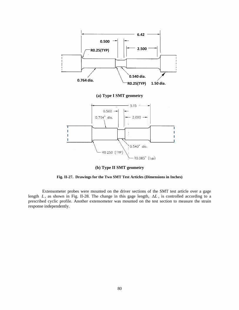
80

(a) Type I SMT geometry

(b) Type II SMT geometry

Fig. II-27. Drawings for the Two SMT Test Articles (Dimensions in Inches)

Extensometer probes were mounted on the driver sections of the SMT test article over a gage

length L , as shown in Fig. II-28. The change in this gage length, L , is controlled according to a

prescribed cyclic profile. Another extensometer was mounted on the test section to measure the strain

response independently.

0.540 dia.

6.42

2.500

0.500

0.764 dia.R0.25(TYP)

R0.25(TYP)

1.50 dia.

81

Fig. II-28. Test setup of the SMT specimen.

There were seven SMT tests performed. The details of the test conditions are shown in Table II-

10. The cyclic profiles of L prescribed for these tests are shown in Fig. II-29. It is seen that fully

reversed cycles, with tensile hold times at the L peak, were imposed on the SMT test articles. It is also

noted that the displacement rate for case (c) is approximately two orders of magnitude slower than the

other cases.

Table II-10. SMT test conditions and data for Alloy 617

Case Spec.

Geom.

Type

Test

Temp.

(C)

Gage

Length,

L (mm)

L Cyclic

Profile

(see Fig.

II-29)

Hold

Time

(s)

Time per

Cycle (h)

Cycles

to

Failure

Life

Time

(h)

1 Type I 950 127.0 ( a ) 600 0.17 450 76.5

2 Type I 950 127.0 ( b ) 600 0.17 1000 170.0

3 Type I 950 127.0 ( c ) 600 0.50 950 475.0

4 Type I 950 127.0 ( d ) 180 0.05 1050 56.0

5 Type II 950 73.7 ( e ) 600 0.17 370 62.9

6 Type II 950 73.7 ( e ) 600 0.17 350 59.5

7 Type II 950 73.7 ( f ) 600 0.17 940 159.8

L

L

Driver

Section

Test

Section

Driver

Section

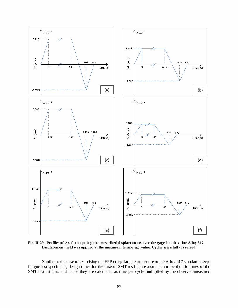
82

Fig. II-29. Profiles of L for imposing the prescribed displacements over the gage length L for Alloy 617.

Displacement hold was applied at the maximum tensile L value. Cycles were fully reversed.

Similar to the case of exercising the EPP creep-fatigue procedure to the Alloy 617 standard creep-

fatigue test specimens, design times for the case of SMT testing are also taken to be the life times of the

SMT test articles, and hence they are calculated as time per cycle multiplied by the observed/measured

(a)

(b)

(c) (d)

(e)

(f)

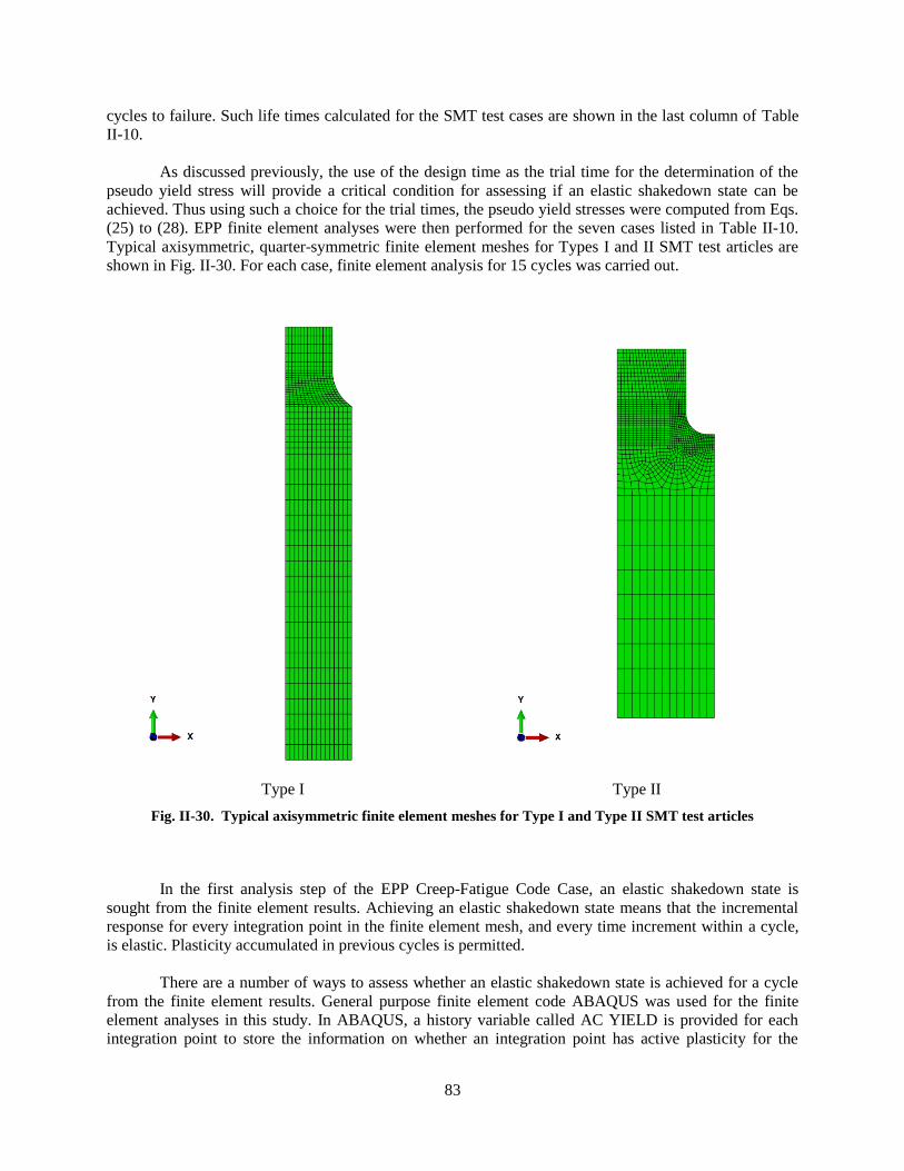
83

cycles to failure. Such life times calculated for the SMT test cases are shown in the last column of Table

II-10.

As discussed previously, the use of the design time as the trial time for the determination of the

pseudo yield stress will provide a critical condition for assessing if an elastic shakedown state can be

achieved. Thus using such a choice for the trial times, the pseudo yield stresses were computed from Eqs.

(25) to (28). EPP finite element analyses were then performed for the seven cases listed in Table II-10.

Typical axisymmetric, quarter-symmetric finite element meshes for Types I and II SMT test articles are

shown in Fig. II-30. For each case, finite element analysis for 15 cycles was carried out.

Type I Type II

Fig. II-30. Typical axisymmetric finite element meshes for Type I and Type II SMT test articles

In the first analysis step of the EPP Creep-Fatigue Code Case, an elastic shakedown state is

sought from the finite element results. Achieving an elastic shakedown state means that the incremental

response for every integration point in the finite element mesh, and every time increment within a cycle,

is elastic. Plasticity accumulated in previous cycles is permitted.

There are a number of ways to assess whether an elastic shakedown state is achieved for a cycle

from the finite element results. General purpose finite element code ABAQUS was used for the finite

element analyses in this study. In ABAQUS, a history variable called AC YIELD is provided for each

integration point to store the information on whether an integration point has active plasticity for the

84

current time increment. Such a condition can be detected easily within ABAQUS internal plasticity

routines. If plasticity is active for the current time increment, AC YIELD has a value of one, and if not,

i.e., the incremental response is elastic, AC YIELD is zero.

Post-processing scripts were developed to extract the information on AC YIELD for every

integration point, every time increment, and every cycle. Using these results, we were not able to

demonstrate elastic shakedown for each of the seven SMT test cases. Plots of the AC YIELD values for a

selected time increment from the 15th cycle are shown in Fig. II-31.

Case 1 Case 2

Case 3

Case 4

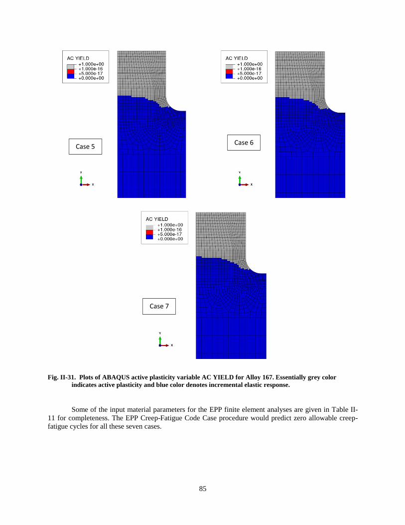
85

Fig. II-31. Plots of ABAQUS active plasticity variable AC YIELD for Alloy 167. Essentially grey color

indicates active plasticity and blue color denotes incremental elastic response.

Some of the input material parameters for the EPP finite element analyses are given in Table II-

11 for completeness. The EPP Creep-Fatigue Code Case procedure would predict zero allowable creep-

fatigue cycles for all these seven cases.

Case 5Case 6

Case 7

86

Table II-11. Material parameters used in the EPP finite element analyses for Alloy 617

Case E (MPa) G (MPa) Sy (MPa) Sr @ Life

Time

(MPa)

PYS @

Life Time,

K'=0.9

(MPa)

Elastic

Shake-

Down?

(Y/N)

Allowable

CF Cycles

from EPP-

CF Code

Case

1 143910 55139 115.7 43.0 38.7 N 0

2 143910 55139 115.7 36.6 33.0 N 0

3 143910 55139 115.7 29.8 26.8 N 0

4 143910 55139 115.7 45.8 41.2 N 0

5 143910 55139 115.7 44.7 40.3 N 0

6 143910 55139 115.7 45.2 40.7 N 0

7 143910 55139 115.7 37.1 33.4 N 0

It is noted that we arrived at the same conclusion of not being able to demonstrate elastic

shakedown when the design factor was not used (i.e., setting 1K ) in establishing the pseudo yield

stress for the EPP finite element analyses.

Application of the Code Case rules to these tests led to the predictions of zero allowable creep-

fatigue cycles, and this simply means that designs under these temperatures and strain cycles are not

viable.

II-5.5 316H Stainless Steel SMT Test

One SMT Type I test article made of 316H stainless steel was tested by Y. Wang of the Oak

Ridge National Laboratory. The details of the test conditions are shown in Table II-12. The cyclic profile

of L prescribed for the 316H test is shown in Fig. II-32.

Table II-12. SMT test conditions and data for 316H SS

Spec.

Geom.

Type

Test

Temp.

(C)

Gage

Length,

L (mm)

Hold

Time

(s)

Time per

Cycle (h)

Cycles

to

Failure

Life

Time

(h)

Type I 815 127.0 600 0.17 400 68

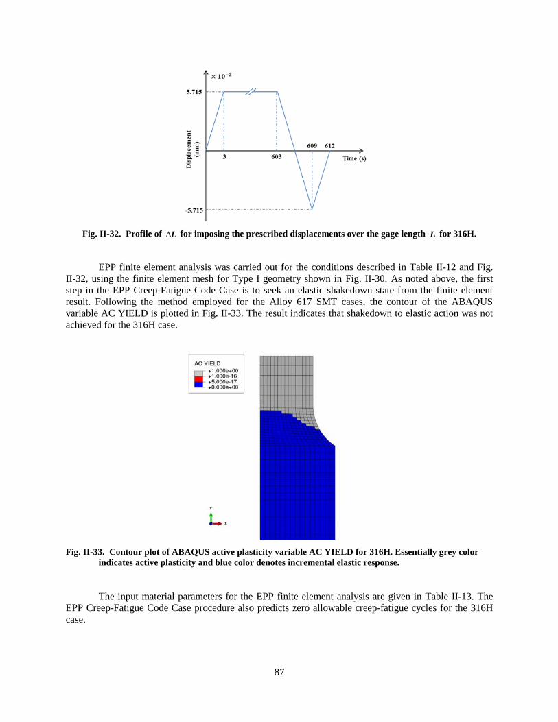
87

Fig. II-32. Profile of L for imposing the prescribed displacements over the gage length L for 316H.

EPP finite element analysis was carried out for the conditions described in Table II-12 and Fig.

II-32, using the finite element mesh for Type I geometry shown in Fig. II-30. As noted above, the first

step in the EPP Creep-Fatigue Code Case is to seek an elastic shakedown state from the finite element

result. Following the method employed for the Alloy 617 SMT cases, the contour of the ABAQUS

variable AC YIELD is plotted in Fig. II-33. The result indicates that shakedown to elastic action was not

achieved for the 316H case.

Fig. II-33. Contour plot of ABAQUS active plasticity variable AC YIELD for 316H. Essentially grey color

indicates active plasticity and blue color denotes incremental elastic response.

The input material parameters for the EPP finite element analysis are given in Table II-13. The

EPP Creep-Fatigue Code Case procedure also predicts zero allowable creep-fatigue cycles for the 316H

case.

88

Table II-13. Material parameters used in the EPP finite element analysis for 316H

E (MPa) G (MPa) Sy (MPa) Sr @ Life

Time

(MPa)

PYS @

Life Time,

K'=0.9

(MPa)

Elastic

Shake-

Down?

(Y/N)

Allowable

CF Cycles

from EPP-

CF Code

Case

127193 48920 75.15 54.08 48.68 N 0

It was found that even when the design factor was not used (i.e., setting 1K ) in establishing

the pseudo yield stress for the EPP finite element analysis, elastic shakedown had not been achieved.

II-5.6 Comparison Based on Allowable Design Life

In the preceding comparisons, the pseudo yield strength was limited by the tabulated yield

strength. The relatively low value of pseudo yield strength prevented elastic shakedown for the high load

levels required to achieve relatively short test durations. In a typical component design, the design life

would be about three orders of magnitude longer than the test duration and the pseudo yield stress would

typically be limited by the creep-rupture strength. Failure to achieve elastic shakedown is a “go, no-go”

type criteria and does not provide a quantitative assessment of the design margin. To get such a

quantitative assessment it is necessary disregard the yield strength and use an extrapolation of the creep-

rupture strength to an allowable design life that is shorter, perhaps significantly shorter, than the test

duration. As the life is shortened the extrapolated creep rupture stress, and hence the pseudo yield

strength, becomes higher. Then, comparing the allowable design life to the measured test life provides a

quantitative design margin assessment.

To implement this procedure, three Alloy 617 test cases were selected with varying loading

amplitudes as shown in Table II-14. Using the ABAQAS finite element model the required pseudo yield

stress for elastic shakedown was determined. From that value, the required time to rupture was determine

taking into account the design factor K’. From the time to rupture and cycle frequency, the allowed

number of cycles was determined. The applicable strain range was determined in accordance with the

code case and the fatigue damage fraction determined from the allowable number of cycles. The

allowable creep damage was then determined from the damage diagram (0.1, 0.1 intercept) for the

calculated fatigue damage. The allowable time was then determined by multiplying the previously

determined required time to rupture by the allowable creep damage fraction. The resulting Alloy 617

design margins are illustrated in Fig. II-34.

Table II-14. Experimental data – Alloy 617 at 950

oC

Test Num. Amplitude

(mils)

Holding time

(s)

Loading time

(s)

Cycle number

to failure

Allowed

lifetime (hrs)

1 1.8 180 3 1050 56

2 2.9 600 3 1000 170

3 4.5 600 3 450 77

89

Fig. II-34. Creep-fatigue code case allowable life comparison to Alloy 617 SMT data

As shown in Table II-15 and Fig. II-35, a similar comparison was done for 316H stainless steel

tested at 815oC.

Table II-15. Experimental data – 316H stainless steel at 815

oC

Test Num. Amplitude

(mils)

Holding time

(s)

Loading time

(s)

Cycle number

to failure

Allowed

lifetime (hrs)

1 1.9 600 3 410 69.7

2 4.5 600 3 13,214 1226

Fig. II-35. Creep-fatigue code case allowable life comparison to 316H stainless steel SMT data

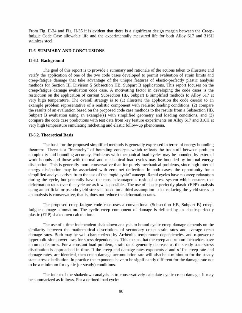
90

From Fig. II-34 and Fig. II-35 it is evident that there is a significant design margin between the Creep-

fatigue Code Case allowable life and the experimentally measured life for both Alloy 617 and 316H

stainless steel.

II-6 SUMMARY AND CONCLUSIONS

II-6.1 Background

The goal of this report is to provide a summary and rationale of the actions taken to illustrate and

verify the application of one of the two code cases developed to permit evaluation of strain limits and

creep-fatigue damage that take advantage of the unique features of elastic-perfectly plastic analysis

methods for Section III, Division 5 Subsection HB, Subpart B applications. This report focuses on the

creep-fatigue damage evaluation code case. A motivating factor in developing the code cases is the

restriction on the application of current Subsection HB, Subpart B simplified methods to Alloy 617 at

very high temperature. The overall strategy is to (1) illustrate the application the code case(s) to an

example problem representative of a realistic component with realistic loading conditions, (2) compare

the results of an evaluation based on the proposed code case methods to the results from a Subsection HB,

Subpart B evaluation using an example(s) with simplified geometry and loading conditions, and (3)

compare the code case predictions with test data from key feature experiments on Alloy 617 and 316H at

very high temperature simulating ratcheting and elastic follow-up phenomena.

II-6.2. Theoretical Basis







simplified analysis arises from the use of the “rapid cycle” concept. Rapid cycles have no creep relaxation

during the cycle, but generally have the most advantageous residual stress system which ensures that

deformation rates over the cycle are as low as possible.. The use of elastic-perfectly plastic (EPP) analysis

using an artificial or pseudo yield stress is based on a third assumption - that reducing the yield stress in

an analysis is conservative, that is, does not reduce the deformation rates.

The proposed creep-fatigue code case uses a conventional (Subsection HB, Subpart B) creep-

fatigue damage summation. The cyclic creep component of damage is defined by an elastic-perfectly

plastic (EPP) shakedown calculation.

The use of a time-independent shakedown analysis to bound cyclic creep damage depends on the

similarity between the mathematical descriptions of secondary creep strain rates and average creep

damage rates. Both may be well-characterized by Arrhenius temperature dependencies, and n-power or

hyperbolic sine power laws for stress dependencies. This means that the creep and rupture behaviors have

common features. For a constant load problem, strain rates generally decrease as the steady state stress

distribution is approached in time. If the creep and damage rates exponents n and n’ for creep rate and

damage rates, are identical, then creep damage accumulation rate will also be a minimum for the steady

state stress distribution. In practice the exponents have to be significantly different for the damage rate not

to be a minimum for cyclic (or steady) conditions.

The intent of the shakedown analysis is to conservatively calculate cyclic creep damage. It may

be summarized as follows. For a defined load cycle:

91

Define a design rupture time t .

Define a temperature dependent “pseudo” yield stress ctS as the lesser of material minimum

yield stress and stress to cause rupture in time t .

Perform a cyclic elastic-plastic analysis to demonstrate shakedown or otherwise of the

component.

If shakedown occurs, then cyclic creep damage is D = design life/t.

II-6.3 Example Problems

II-6.3.1 Representative example

The goal of the representative example is to illustrate the code case(s) application to a realistic

geometry and loading conditions. The selected geometry is a spherical head with an integrally reinforced

nozzle with a flush ground connecting weld. The applied loads are internal pressure and shear and

moment loads on the nozzle. Cyclic and sustained loading conditions are evaluated with imposed thermal

transients. The material is 316H stainless steel.

The evaluation of the implementation of creep-fatigue code case was successful. The

implementation requires shakedown to elastic behavior with trial-and-error finite element EPP using a

pseudo yield strength based on a creep-rupture strength target life iterated with successively longer values

until the combined creep damage and fatigue damage satisfy the damage criteria envelope in Subsection

HB, Subpart B. If shakedown cannot be achieved within the allowable creep and fatigue damage

envelopes, then the applied loadings are not acceptable. The creep damage calculation is a bounding value

applicable to all points in the structure and not a specific value for each location. The creep damage value

is combined with the maximum value of the fatigue damage to bound the total damage for the component.

Two FEA models were used, with and without the weldment included. There are slight

differences in the results due to the influence of the lower pseudo yield strength in the weldment caused

by the weld strength reduction factor. The weldment model Level A & B Composite Cycle analysis with a

target creep damage of 0.95 passes after 3 pseudo-cycles. The base metal only model passes with a target

creep damage of 0.90, also after 3 pseudo cycles. For the weldment model, the total creep-fatigue damage

is 0.954 and the allowable creep-fatigue damage is 0.995, which is sufficiently greater than the calculated

value. This places the creep-fatigue damage within the HBB-T-1420-2 creep-fatigue interaction

envelope, thus meeting the criteria for creep-fatigue interaction for the base metal. For the base metal only

model, the corresponding total and allowable damages are 0.904 and 0.995 respectively. In the weld

region, the corresponding values of total damage and allowable damage are 0.958 and 0.988 respectively.

The base metal only creep-fatigue evaluation for the Level A & C Composite Cycle with a target

creep damage of 1.0 does not pass after 20 pseudo-cycles. The change in plastic strain after each pseudo-

cycle is 0.28% indicating that stable ratcheting continues and shakedown does not occur. Further

reduction of the target creep damage will only produce weaker pseudo-yield stresses, resulting in even

more severe ratcheting.

II-6.3.2 Creep-fatigue code case to Subsection HB, Subpart B comparison

Creep-fatigue damage was evaluated to compare the results from the current Subsection HB,

Subpart B procedures to the results from the proposed creep-fatigue code case using elastic-perfectly

plastic methods. The evaluation was done using a relatively thick wall cylinder, 16 inches OD with 2

inches wall thickness. The steady state condition is an inner wall temperature of 1235 oF and an outer wall

92

temperature of 1075 oF. The heat flux is periodically cycled to zero while maintaining the inner wall

temperature constant such that the outer wall temperature equals the inner wall temperature. The material

is 316H stainless steel. The estimated allowable life from the current Subsection HB, Subpart B procedure

is 1430 hrs as compared to an estimated life of approximately 10,000 hrs using the proposed EPP creep-

fatigue code case.

II-6.4 Bounding Theory Example Calculations

Analytic solutions were developed for the example of a creep-fatigue test specimen subjected to

cyclic, displacement controlled loading. Using these analytic solution it was demonstrated that the creep

damage from the rapid cycle/EPP solution would bound the creep damage calculated from a time fraction

damage summation using the calculated stress/time history. These detailed analytic solutions for the

creep-fatigue test thus demonstrate the conservatism of the EPP code case methodology for a simplified

yet realistic example.

II-6.5 Experimental Results

Experiments were conducted on standard creep-fatigue test specimens and key feature test articles

that were modified from standard creep-fatigue test specimens to replicate the follow-up and stress and

strain redistribution characteristics of realistic components and loading at elevated temperature. When the

EPP creep-fatigue methodology was applied to evaluate the test results it was shown that the applied test

loading did not result in elastic shakedown; thus demonstrating that the code case is conservative in that it

would not permit the test loadings in a design application.

II-6.6 Conclusions

As summarized above, the creep-fatigue code case, (1) can be implemented on a representative

component configuration with realistic loading conditions, (2) provides comparable results to current

Subsection HB, Subpart B procedures at moderate creep temperatures, and, (3) is conservative with

respect to the evaluation of creep-damage on experiments with Alloy 617 and 316H stainless steel at very

high temperatures. Also, the validity of the bounding theory that forms the basis of the creep-fatigue code

case based on elastic-perfectly plastic analysis concepts has been demonstrated analytically

93

II-APPENDIX A

The EPP elastic shakedown solution with stress cycle can be given as

1

2 1

( ) / 2 / 2E E

(A29)

The damage accumulation over a half-cycle from the E-PP elastic shakedown solution, eppD , is given by:

12

n

eppD k

(A30)

For the case of steady cyclic-creep, the governing equations are

( )c

n

c

E

k

(A31)

Under the constant strain rate condition, 0 , the stress relaxation behavior can be obtained from

0

( )t

n

dEkt

(A32)

where 0 at 0t . Integrating Eq. (A32), we find

1 1

0

1( )

1

n nt Ektn

(A33)

and

1

11

0( ) (1 )nnt n Ekt

(A34)

The stress relaxation expression in Eq. (A34) admits the limit

0

1lim ( ) exp( )n

t Ekt

(A35)

The damage accumulation over a half-cycle from the steady cyclic-creep solution, cD , is given by

/2

0

( )n

cD k t dt

(A36)

Substituting the stress relaxation expression from Eq. (A34) into Eq. (A36), we find

1 1

02( )

( 1 )

n n n n

c

kD

kE n n

(A37)

94

The condition for steady cyclic-creep solution is

0 2( ) E E (A38)

and it is illustrated in Fig. A1.

Fig. A1. Steady cyclic creep condition (in blue) and EPP elastic

shakedown condition (in red)

Using Eqs. (A30) and (A37), the damage ratio between the steady cyclic-creep solution and the

EPP elastic shakedown solution is

1 1

02

1

( )1

( 1 ) / 2

n n n n

c

n

epp

D

D kE n n

(A39)

From Eqs. (A29) and (A38), we find

1 0 2

1( )

2

(A40)

and from Eqs. (A33) at half cycle, i.e., at / 2t , we get

11

0 2

1( )

2 1

nnEkn

(A41)

Substituting Eqs. (A40) and (A41) into Eq. (A39), the damage ratio becomes

11

0 2

11

0 02 2

( )( 1)2

( 1 ) ( ) ( )

n nn nn

c

n nnepp

D n

D n n

(A42)

1 / 2E

( / 2)

0

95

Under the condition of n n the damage ratio is further reduced to

0 2

1 1

0 02 2

( )2 ( 1)

( ) ( )

nc

n nnepp

Dn

D

(A43)

To simplify the notation, we introduce the stress ratio s as

0 2/ ( )s (A44)

The damage ratio then becomes

1

1

2 ( 1)( 1)

1 1

n n

c

nnepp

D n s s

D s s

(A45)

We now investigate the behavior of the damage ratio as a function of n and s . Let

1

1

2 ( 1)( 1)( , )

1 1

n n

nn

n s sf n s

s s

(A46)

The result in Eq. (A41) implies that as 1s the creep deformation becomes vanishingly small and in the

limit of 1s the creep deformation is frozen (e.g., 0k ) and the steady cyclic-creep stress state is

reduced to the EPP elastic shakedown solution. This can be seen from Fig. A1. The Taylor series

expansion of ( , )f n s about 1s gives

2 3 4

0 0 0

1( , ) 1 ( 1) ( 1) ( 1) , ( 1)

24f n s a s a s O s a n n (A47)

where ( )O is the order symbol. This confirms that ( , ) 1f n s as 1s . Also, for values of s slightly

larger than one, Eq. (A47) shows that ( , ) 1f n s . Hence the damage accumulation from the steady cyclic-

creep solution for small amounts of stress relaxation over the half-cycle is less than the damage calculated

from the EPP elastic shakedown solution.

For large s , we find from Eq. (A46) that

1

2 ( 1)( , ) ~

1

n

n ns

nf n s

s

(A48)

so 0f in the limit as s . This is the case when the stress relaxation from the steady cyclic-creep

solution over the half-cycle is complete, and the damage accumulation is vanishingly small as compared

with the corresponding damage accumulation from the EPP elastic shakedown solution.

We now study the behavior of ( , )f n s near 1n . A Taylor series expansion of ( , )f n s about

1n gives

96

2

0 1( , ) ( 1) ( 1)f n s b b n O n (A49)

where

2 3 4

0

2( 1) 1 11 ( 1) ( 1) ( 1)

( 1) ( ) 12 12

sb s s O s

s n s

(A50)

2 3 4

1

( 1) 2 (2) ( ) 2 ( 1) 1 1( 1) ( 1) ( 1)

( 1) ( ) 8 8

s n n s n sb s s O s

s n s

(A51)

Hence 0f b as 1n and Eq. (A50) shows that

0 1b .

From the above analysis, it can be concluded that the damage ratio is one at 1n and 1s . It

decays from one to zero as n and s are increased. A three-dimensional plot of ( , )f n s for 1 10n

and 1 10s is shown in Fig. A2.

Fig. A2. 3D plot of damage ratio as function of n and s.

In summary, under the assumption that the creep rate and damage rate have the same stress

dependency, i.e., n n , it is shown that the damage accumulation over a half-cycle of creep-fatigue

straining as determined from an elastic, power-law creep model is bounded by, or less than, the

corresponding damage accumulation from the EPP elastic shakedown solution:

0 1c

epp

D

D (A52)

97

II-APPENDIX B: DRAFT EPP CREEP-FATIGUE CODE CASE

The draft EPP creep-fatigue code case is presented in this appendix. It is anticipated that revision

will be made to this draft to address comments as the Code committee approval process proceeds.

Code Case XXXX. Calculation of Creep-Fatigue for Division 5 Class A Components at Elevated

Temperature Service Using Elastic-Perfectly Plastic Analysis.

Inquiry: What alternative rules may be used for the calculation of creep-fatigue damage in compliance

with HBB-3252 and Appendix HBB-T.

Response: Fatigue and creep damage may be evaluated for the following materials using elastic-perfectly

plastic material models instead of the procedures of HBB-T-1420, HBB-T-1430 and HBB-T-1715 when

performed in accordance with the requirements of this Code Case.

Type 304 SS and 316 SS per Table HBB-I-14.1(a)

1. General Requirements.

Except as identified herein, all requirements of Section III, Division 5, Subsection HB, Subpart B apply to

components designed in accordance with this Code Case.

The design methodology employed for evaluation of creep damage is based on elastic shakedown

analyses using an elastic-perfectly plastic material model, small strain theory and a “pseudo” yield

strength selected to bound creep damage. In this Code Case, “shakedown” refers to the achievement of

cyclic elastic behavior throughout the part, based on real or pseudo yield properties. In this Code Case the

term “pseudo yield stress” refers to a temperature dependent minimum stress-to-rupture value based on a

selected trial time duration, not to exceed the yield strength of the material at temperature and is explicitly

defined in paragraph 4.2. of this Code Case. Guidance on shakedown analysis is provided in Appendix 1.

The combination of Levels A, B, and C Service loadings shall be evaluated for accumulated creep and

fatigue damage, including hold time and strain rate effects. For a design to be acceptable, the creep and

fatigue damage at each point in the component shall satisfy the following relation:

c fD D D (53)

where

D = total creep-fatigue damage, as limited by FIG. HBB-T-1420-2

cD = creep damage, as determined in paragraph 4, below, of this Code Case

fD = fatigue damage, as determined in paragraph 5, below, of this Code Case

(a) This design methodology is not applicable to structures where geometrical nonlinearities exist, e.g.

canopy and omega seals.

(b) The stamping and data reports shall indicate the case number and applicable revision.

2. Load Definition.

Define all applicable loads and load cases per HBB-3113.2 Service Loadings.

2.1. Composite cycle definition.

For the purpose of performing an elastic-perfectly plastic shakedown analysis, an overall cycle must be

defined that includes all relevant features from the individual Level A, B and C Service Loadings

identified in the Design Specification. Relevant features include, as a minimum, the time-dependent

sequence of thermal, mechanical and pressure loading including starting and ending conditions. Such an

overall cycle is defined herein as a composite cycle subject to the following requirements.

98

2.1.1. An individual cycle as defined in the Design Specifications cannot be split into individual cycles to

satisfy these requirements.

2.1.2. Except as described in 2.1.3. below, a single cycle from each Level A, B and C Service Loading

cycle type shall be included in the composite cycle for evaluation of creep-fatigue.

2.1.3. Level C Service Loadings may be combined with the applicable Level A and B Service Loadings to

define a composite cycle(s) to be evaluated separately from the cycle defined in 2.1.2. Multiple composite

cycles that include Level C Service Loadings may be defined for separate evaluation. The total number of

Level C Service Loading cycles shall not exceed 25.

3. Numerical Model.

Develop a numerical model of the component, including all relevant geometry characteristics. The model

used for the analysis shall be selected to accurately represent the component geometry, boundary

conditions, and applied loads. The model must also be accurate for small details, such as small holes,

fillets, corner radii, and other stress risers. The local temperature history shall be determined from a

thermal transient analysis based on the thermal boundary conditions determined from the loading

conditions defined in paragraph 2.

4. Calculation of Creep Damage.

Perform a shakedown analysis for each of the composite cyclic histories defined in paragraph 2.1. Each of

these cyclic histories must be shown to shakedown based on the pseudo yield stress defined in paragraph

4.2. Additional requirements for welds are found in paragraph 6.

4.1. Step 1: Define designt as the total time duration for all Level A, B, and C Service Loadings when the

temperature is above the range covered by Tables 2A, 2B, and 4 of Section II, Part D.

4.2. Step 2: Select a trial time duration, dT in order to define a pseudo yield stress,

dTS , at each location,

using the temperature determined from the transient thermal analysis. This pseudo yield stress is equal to

the lesser of the quantities defined below in 4.2.1. and 4.2.2.

4.2.1. The yield strength yS given in Table I-14.5;

4.2.2. rS , where

rS is the minimum stress to rupture in time dT from FIGS. HBB-I-14.6 multiplied by the

factor, K , from Table HBB-T-1411-1 using the tabulated values for Elastic Analysis.

4.3. Step 3: Perform a cyclic elastic-perfectly plastic analysis for each composite cycle defined in

paragraph 2 above with temperature-dependent pseudo yield stress dTS . The assessment temperature shall

be taken as the local instantaneous temperature at every location in the numerical model of the

component. If shakedown occurs, that is, cycles with eventual elastic behavior everywhere, proceed to

Step 4. If shakedown does not occur, the applied loading does not meet the requirements of this Code

Case.

4.4. Step 4: The maximum creep damage over the structure for the composite cycle under consideration

is:

design

c

d

tD

T

(54)

The above value of cD is used to evaluate total damage in Eq. (53). If the pseudo yield strength in 4.2.

Step 2 is governed by the yield strength as defined in 4.2.1., then the trial time duration for use in Eq. (2)

is given by the time at which the minimum stress to rupture is equal to the yield strength; r yS S . Linear

extrapolation of rS values corresponding to the two longest tabulated times can be used to obtained the

trial time duration when necessary.

99

4.4.1. Steps 2, 3 and 4 may be repeated to revise the value of cD by selecting alternative values of the

trial time duration, dT . Longer values of

dT will reduce the calculated creep damage. However, these

longer values will lead to lower values of the pseudo yield stress, dTS , which will make shakedown more

difficult.

5. Calculation of Fatigue Damage.

The fatigue damage summation, fD , in Eq. (53) is determined in accordance with Steps 1 through 3

below. Additional requirements for welds are found in paragraph 6.

5.1. Step 1: Determine all the total, elastic plus plastic, strain components for the composite cycle at each

point of interest from the shakedown analysis performed in Step 3 of paragraph 4 above.

5.2. Step 2: Calculate the equivalent strain range in accordance with HBB-T-1413, or HBB-T-1414 when

applicable, with Poisson’s ratio * 0.3 .

5.3. Step 3: Determine the fatigue damage for each composite cycle from the expression:

( )

j

f

j d j

nD

N (55)

where

jn = number of applied repetitions of cycle type, j

( )d jN = number of design allowable cycles for cycle type, j , determined from one of the design

fatigue curves from FIGS. HBB-T-1420-1 corresponding to the maximum metal temperature

occurring during the cycle.

The value of fD used to evaluate total damage in Eq. (53) is the maximum value at any location in the

numerical model.

6. Weldments.

Implementation of the evaluation of creep-fatigue damage in paragraphs 4 and 5 above for weldments

requires additional consideration.

6.1. In the weld region, the pseudo yield stress value defined by dT in 4.2.2. is reduced further by

multiplying the value of rS for the base metal by the applicable weld strength reduction factor from Table

HBB-I-14.10.

6.2. The number of allowable cycles, d jN , in the weld region is one half the number of allowable

cycles from FIGS. HBB-T-1420-1 for base materials.

6.3. The requirements for analysis of geometry of subparagraph HBB-T-1714 are applicable for

satisfaction of the requirements of this Code Case.

6.4. The thermal/physical properties of weldments may be assumed to be the same as the corresponding

base metal for the base metal - weld combinations listed in Table HBB-I-14.10.

6.5. Weld region model boundaries.

The weld shown in Figure 1 represents a general full-penetration butt weld in a shell. Other weld

configurations are needed for construction of an elevated temperature component in accordance with

Subsection HB, Subpart B. Article HBB-4200 refers to various Division 1, Subsection NB-4000

paragraphs for weld configurations and requirements. These Subsection NB weld configurations are

represented by the shaded region.

100

Figure 1 shows a full-penetration butt weld as an example. As shown, 1w and

2w , as needed to define the

weld region for use of this Case, are approximations consistent with the specified weld configuration and

parameters. The specified weld region must include applicable stress concentrations in accordance with

the requirements for analysis of geometry of Subparagraph HBB-T-1714.

Figure 1. Weld region model boundaries

6.5. Dissimilar metal welds.

6.5.1. The requirements for dissimilar metal welds are in the course of preparation.

Appendix 1. Shakedown Analysis.

The steps to perform a shakedown analysis to calculate bounding cyclic creep damage are as follows:

i) Define Composite Cycle Load Time-Histories and Step(s).

a. It may consist of histories of mechanical loads, pressure loads, displacements, temperatures and

thermal boundary conditions.

b. Time-independent parts of the cycle may be truncated because the elastic-perfectly plastic

analysis is not time dependent.

c. The cycle should not have discontinuities. Discontinuities arising from the selection of the


transition from one operating state to the next.

d. Subject to the requirements in (ii), the composite cycle time does not affect the result of the

shakedown analysis.

e. Temperatures, thermal boundary conditions, boundary displacements and mechanical loads over a

cycle should be cyclic; that is, begin and end at the same value.

f. A single analysis step may represent one cycle. Dividing a single cycle into more than one step to

facilitate definition of the load cycle, and to ensure that maximum loads are analyzed, is often

helpful.

ii) Define Analysis Types.

a. A sequentially coupled thermal-mechanical analysis of the composite cycle may be performed.

First, a thermal analysis is performed to generate temperature histories. Next, the mechanical

analyses are performed using these temperature histories as inputs. Care must be taken that times

in the mechanical analysis step and in the previous thermal analysis are the same or do not

conflict, depending on the requirements of the analysis software.

b. Alternatively, a coupled thermal-mechanical analysis may be performed. The composite

temperature history to be used in the mechanical analysis should be cyclic, that is the beginning

and end temperature distributions should be the same.

101

iii) Define Material Properties.

a. For thermal analyses, density, temperature-dependent specific heat and conductivity will

generally be required.

b. For the mechanical analyses, the temperature-dependent properties required are elastic modulus,

Poisson’s ratio and mean expansion coefficient. Density may also be required.

iv) Perform Analyses.

a. Perform an elastic-plastic cyclic mechanical and thermal stress analysis using the temperature-

dependent yield stress defined above. Enough cycles are required to demonstrate shakedown or

otherwise.

b. Care must be taken to ensure that the analysis deals with all the changes within a cycle. Elastic-

plastic routines increase increment size where possible, and may miss a detail in the loading. A

conservative limit to maximum increment size can address this problem, or division of the cycle

into more than one step as in paragraph (i)(f) of this appendix.

v) Shakedown.

(a)Shakedown is defined in this Code Case as eventual elastic behavior everywhere in the model. Failure

to shakedown may be identified by plotting histories of equivalent plastic strain.

102

REFERENCES

Carroll, L. J., Cabet, C., Carroll, M. C., and Wright, R. N., (2010), “The Role of Environment on High

Temperature Creep–Fatigue Behavior of Alloy 617,” Proceedings of the ASME Pressure Vessel and

Piping Division Conference, Bellevue, WA, July 18–22, PVP2010-26126, American Society of

Mechanical Engineers, New York, NY.

Carter, P., (2005a), “Analysis of cyclic creep and rupture. Part 1: Bounding theorems and cyclic reference

stresses,” Int. J Press & Piping, Vol. 82, pp. 15-26.

Carter, P., (2005b), “Analysis of cyclic creep and rupture. Part 2: Calculation of cyclic reference stresses

and ratcheting interaction diagrams,” Int. J Press & Piping, 82, pp. 27-33.

Carter, P., Jetter, R., Sham, T.-L., (2012a), “Application of Elastic-Perfectly Plastic Cyclic Analysis to

Assessment of Creep Strain”, PVP 2012 – 28082, American Society of Mechanical Engineers, New

York, NY.

Carter, P., Jetter, R., Sham, T.-L., (2012b), “Application of Shakedown Analysis to Evaluation of Creep-

Fatigue Limits”, PVP 2012-28083, American Society of Mechanical Engineers, New York, NY.

Corum, J.M., and Blass, J.J., (1991), Rules for Design of Alloy 617 Nuclear Components to Very High

Temperatures, ASME PVP Vol. 215, p.147, American Society of Mechanical Engineers, New York,

NY.

Eno, R., G.A. Young, and T.-L. Sham, (2008), “A Unified View of Engineering Creep Parameters,”

Proceedings of the ASME 2008 Pressure Vessels and Piping Division Conference, Chicago, Illinois,

July 2008, Paper No. PVP2008-61129, American Society of Mechanical Engineers, New York, NY

Goodall, I.W., Leckie, F.A., Ponter, A.R.S., Townley, C.H.A, (1979), “The Development of High

Temperature Design Methods Based on Reference Stresses and Bounding Theorems,” ASME Journal

of Engineering Materials and Technology, Vol. 101.

Hollinger, G. L. and Pease, D., J., (2014), “Comprehensive Report For Proposed Elevated Temperature

Elastic Perfectly Plastic (EPP) Code Cases Representative Example Problems”, 20362-R-001 Rev.3,

Becht Engineering, Liberty Corner, NJ.

Jetter, R.I., (1998), “An Alternate Approach to Evaluation of Creep-Fatigue Damage for High

Temperature Structural Design,” PVP-Vol. 5 Book No. H01146 – 1998, pp. 199-205, American

Society of Mechanical Engineers, New York, NY.

Pitts, D.R., and Sissom, L.E., (1998) Schaum’s Outline of Theory and Problems of Heat Transfer, 2nd

Ed., McGraw Hill.

Roark, R. J., and Young, W. C., (1989) Roark’s Formulas for Stress and Strain, 6th ed., McGraw-Hill,

New York.

Swindeman, R., Robinson, D., Williams, B. and Thomas, D., (1982) “Two-Bar Thermal Ratcheting

Experiments on 2¼Cr-1Mo steel” ORNL/TM-8001.

103

The American Society of Mechanical Engineers, Boiler and Pressure Vessel Code, Section II, Part D,

(2013) “Materials, Properties,” American Society of Mechanical Engineers, New York, NY.

The American Society of Mechanical Engineers, Boiler and Pressure Vessel Code, Section III, Division 5,

Subsection HB, Subpart B, (2015), “Class A Components in Elevated Temperature Service,”

American Society of Mechanical Engineers, New York, NY.

Wang, Y, Jetter, R., and Sham, T.-L., (2013) “Progress Report on Creep-Fatigue Design Method

Development Based on SMT Approach for Alloy 617”, ORNL/TM-2013/349, Oak Ridge National

Laboratory, Oak Ridge, TN.

Wang, Y, Jetter, R., and Sham, T.-L., (2013) “Progress Report on the Development of Test Procedure for

the Two-bar Thermal Ratcheting Experiment for Alloy 617” ORNL/TM-2013/318.

104

Page Intentionally Blank

ORNL/TM-2015/487

DISTRIBUTION LIST

Name Affiliation Email

Corwin, W. DOE [email protected]

Sink, C. DOE [email protected]

Grandy, C. ANL [email protected]

Hill, R.N. ANL [email protected]

Li, M. ANL [email protected]

Majumdar, S. ANL [email protected]

Croson, D. INL [email protected]

Petti, D. INL [email protected]

Wright, J. INL [email protected]

Wright, R.N. INL [email protected]

Lara-Curzio, E. ORNL [email protected]

Sham, T.-L. ORNL [email protected]

Wang, H. ORNL [email protected]

Wang, Y. ORNL [email protected]

Hollinger, G. Becht Engineering Co., Inc. [email protected]

Pease, D. Becht Engineering Co., Inc. [email protected]

Carter, P. Stress Engineering Services Inc. [email protected]

Jetter, R.I. Consultant [email protected]

Pu, C. University of Tennessee [email protected]

Documents

Report on FY15 Alloy 617 Code Rules Development