Report on Study of Electrical Component Corrosion Related

to Problem Drywall

Andrew Trotta Mark Gill

Division of Electrical Engineering Directorate for Engineering Sciences

U.S. Consumer Product Safety Commission

March 2011 This report was prepared by CPSC staff and has not been reviewed or approved by, and may not necessarily reflect the views of, the Commission.

-2-

Introduction Attached at Tab A is Sandia National Laboratories’ (Sandia or SNL) final report (Report on Accelerated Corrosion Studies of Electrical Components) on their analysis of corrosion of electrical components exposed to selected contaminant gasses at elevated temperature and humidity to simulate 40 years of exposure to the approximate conditions present in homes with problem drywall. This work was undertaken as part of the U.S. Consumer Product Safety Commission (CPSC) staff’s multitrack plan to assess the health and safety impacts of problem drywall. Background

In April 2009, CPSC Engineering staff developed a plan to study whether problem drywall-related corrosion could result in degradation that could affect the performance of electrical components and/or pose a risk of electric shock or fire. To assist in the execution of this plan, CPSC staff tasked the Materials Science and Engineering Center at SNL, through an interagency agreement with the Department of Energy/National Nuclear Security Administration (1) to perform detailed metallurgical analyses of electrical components harvested from homes constructed with problem drywall, and (2) to assess long-term effects by conducting accelerated corrosion testing on new residential electrical components. In November 2009, SNL released a report, Interim Report on the Analysis of Corrosion Products on Harvested Electrical Components (Glass et al., 2009), on the preliminary analysis of six receptacles that had been collected by CPSC staff from affected homes in Virginia and Florida. This report is attached as an appendix to the CPSC staff report, Interim Report on the Status of the Analysis of Electrical Components Installed in Homes with Chinese Drywall (Gill and Trotta, 2009).

Sandia’s November 2009 preliminary analysis of six standard duplex receptacles that had

been harvested from affected homes indicated that the accumulation of copper sulfide corrosion was evident visually on metal surfaces that were exposed to air in homes in which problem drywall was installed, but that the corrosion layer was relatively thin compared to the overall volume of the conductors. Secure metal-to-metal contact surfaces were not corroded. In addition, none of the harvested samples exhibited signs of prefire conditions, such as overheating or arcing. Although, the relatively fast accumulation of corrosion on the components is undesirable, there did not appear to be a short-term effect on electrical safety. In addition, Sandia indicated that the copper sulfide that was observed on the corroded parts is a stable compound that would not continue to grow in the absence of reactive sulfur gases such as hydrogen sulfide.

The rate and nature of corrosion on the components that had been harvested from the six

houses after approximately three years of exposure to problem drywall led Sandia to characterize the local environment as Battelle Class III to IV (Abbott, 1988), comparable to a corrosive industrial environment as opposed to a typical residential environment. One point of significance of this classification is that it defined the test conditions for the evaluation of the long-term safety effects due to corrosion through the use of accelerated corrosion testing. Accelerated corrosion testing involves placing the components under evaluation in a chamber in which the corroding gas is combined with additional gases to accelerate the reaction processes, mixed and circulated through the chamber. Eventually, Sandia opted to test the components at

-3-

the Class IV level. These tests commonly are referred to as mixed-flowing gas (MFG) tests. ASTM B827, Standard Practice for Conducting Mixed Flowing Gas (MFG) Environmental Tests, provides guidance for conducting this type of laboratory accelerated-corrosion testing.

Another critical test parameter involved identifying the primary corroding gas. This had

been identified largely by outside parties studying Chinese drywall as H2S; but CPSC staff sought to identify independently what the corroding gas was by sponsoring laboratory chamber studies, as well as in-home air quality investigations. Staff contracted with Lawrence Berkeley National Laboratory (LBNL) for measurement of chemical emissions from 30 samples of drywall products obtained as part of the drywall investigation. According to LBNL (Maddalena et al., 2010), the highest concentration gas was H2S, but many other reactive sulfur gases were also present in the samples with high emissions. The top 10 reactive sulfur-emitting drywall samples were from China. The patterns of reactive sulfur compounds emitted from drywall samples showed a clear distinction between the Chinese drywall samples manufactured in 2005/2006, and Chinese and North American samples with manufacture dates of 2009, which did not emit reduced sulfur gases at particularly noteworthy levels. The data linking problem drywall with H2S emissions was augmented by Environmental Health & Engineering’s CPSC-sponsored 51-home study (Environmental Health & Engineering, 2010), which correlated that the corrosion was attributable to problem drywall. Homes with imported drywall had significantly greater H2S concentrations compared to control homes in the study.

Sandia staff verified with William Abbott at Battelle that two weeks of exposure in the

mixed flowing gas chamber was approximately equivalent to 10 years of actual exposure. Sandia’s November 2009 preliminary analysis provided a snapshot of the relatively short-term in-situ effects of the drywall-related corrosion in approximately three-years-old houses whereas the MFG chamber tests would help answer the question of what possible long-term effects could take place if the drywall remained in place. Most electrical system components, particularly passive ones like standard duplex receptacles, are extremely durable, subject to a wide variation in their frequency of usage, and they have no specified service life or recommended replacement schedule. However, CPSC staff’s recommendation in the CPSC Guide to Home Wiring Hazards (CPSC Publication No. 518) is that homeowners have their electrical systems inspected, at the very least, every 40 years. Seeking to balance the selection of the test duration that was both conservative and reasonable in assessing the long-term effects of the drywall-related corrosion (especially without knowing how long the drywall may off-gas), CPSC staff selected 40 years of aging, which equated to eight weeks of corrosive exposure of the components in the test chamber.

CPSC staff chose to cycle the components electrically during the exposure period in the

chamber to provide thermally-driven stresses of the corrosion product (due to differences in the thermal expansion properties of the metal conductors and the corrosion products). Sandia staff used the load cycling to assess corrosion-induced functional impacts while components were undergoing exposure by measuring voltage drops across the circuits. An increase in voltage drop over the course of testing would signal degradation of the connection resistance within the circuit. Running the components under a load involved selecting a suitable load current based on the 15-ampere (A) rating of the components in the circuit and a duty cycle to define the on/off period of the load. Class IV conditions require the chamber temperature to be held at 50°C.

-4-

Circuit breakers are calibrated to carry 100 percent current at 40°C, so derating1 the current-carrying capacity of the circuit breaker under this elevated ambient temperature was required to guard against nuisance tripping. On this basis, CPSC staff decided to load the circuits at 80 percent of the handle rating of the circuit breaker (the breakers to be placed in the chamber were rated for 15 A) and because 80 percent also complies with 2008 National Electrical Code Article 210.23(A)(1).2

For a 15-ampere-rated circuit, this corresponds to 12 A. Sandia elected to use portable halogen work lights as the electrical loads for each of three separate circuits. Three work lights, rated 500 Watts (W) each (at 125 volts), were connected electrically in parallel and then attached to each circuit for a rated total of 1500 W. CPSC staff selected a 50 percent duty cycle with 10 minutes on, and 10 minutes off, allowing time for the circuit components to come up to temperature when connected to the electrical loads, and to return to ambient temperature when disconnected. The test circuits were constructed by a qualified technician in accordance with common electrical wiring practices and manufacturer specifications, to the extent practicable.

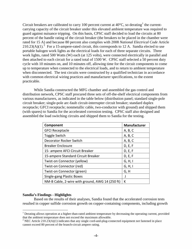
While Sandia constructed the MFG chamber and assembled the gas control and distribution network, CPSC staff procured three sets of off-the-shelf electrical components from various manufacturers, as indicated in the table below (distribution panel; standard single-pole circuit breaker; single-pole arc-fault circuit-interrupter circuit breaker; standard duplex receptacle; GFCI receptacle; nonmetallic cable, two-conductor with ground) and shipped them (with spares) to Sandia for the accelerated corrosion testing. CPSC staff also designed and assembled the load switching circuits and shipped them to Sandia for the testing.

Component Manufacturer GFCI Receptacle A, B, C Toggle Switch A, B, C Decorator Rocker Switch A, B, C Breaker Enclosure D, E, F 15- ampere AFCI Circuit Breaker D, E, F 15-ampere Standard Circuit Breaker D, E, F Twist-on Connector (yellow) G, H, I Twist-on Connector (red) G, H, I Twist-on Connector (green) G, H Single-gang Plastic Boxes J NM-B Cable, 2-wire with ground, AWG 14 (250 ft) K

Sandia’s Findings - Highlights

Based on the results of their analyses, Sandia found that the accelerated corrosion tests resulted in copper sulfide corrosion growth on copper-containing components, including growth

1 Derating allows operation at a higher-than-rated ambient temperature by decreasing the operating current, provided that the ambient temperature does not exceed the maximum allowable. 2 NEC Article 210.23(A)(1) indicates that any single cord-and-plug-connected equipment not fastened in place cannot exceed 80 percent of the branch-circuit ampere rating.

-5-

inside non-hermetically-sealed components (receptacles, breakers, and twist-on connectors), with reduced growth in areas of reduced availability to gas diffusion.

Sandia’s scientists also observed that insulation on the type NM (nonmetallic) power cables tested in the ACT chamber appeared to be very effective in protecting the underlying copper wire. Whenever they removed electrical insulation for inspection of the underlying copper surface, they saw no evidence of wire corrosion. They asserted that their observations on this in particular cannot be extrapolated to a 40-year lifetime, but that the fact remains that the insulated wire, when exposed to a very aggressive environment, did not suffer corrosion beneath the wire insulation.

With respect to electrical characteristics and possible hazardous conditions, Sandia reported that their testing and materials characterization measurements revealed:

• no growth between surfaces that retained physical contact during testing; • no manifestations of fire or overheating; • no significant detectable changes in circuit resistance (measured via voltage drop); and • no significant degradation of wire cross sectional area.

Conclusions

After exposure to the harsh corrosive conditions of the Battelle Class IV environment for eight weeks, roughly equivalent to 40 years of exposure to conditions representative of a house with problem drywall, corrosion of the electrical components was observed, which was consistent with Sandia’s examination of harvested components and the effects from problem drywall reported to the CPSC by thousands of consumers. Sandia staff did not observe any acute or long-term safety events, such as smoking or fire, during the course of the experiment. Accordingly, it is the belief of CPSC staff and Sandia that even simulated long-term exposure of wiring and other electrical components to hydrogen sulfide gases does not indicate a safety hazard to the home’s electrical systems.

While no fire, smoking, or other safety events occurred during the course of this experiment, CPSC staff and Sandia are mindful of the limited scope and controlled conditions of this experiment. The experiment does not, and could not, possibly capture every permutation of conditions, wiring, installation, brands, environmental conditions, and other possible confounding factors that are actually present in the affected houses. For example, it is widely known (Dini, 2008), and CPSC engineers have often observed, that electrical system components in homes may be installed with substandard workmanship, and this may affect connection resistance and performance. Sandia’s testing was performed at manufacturers’ recommended torque installation levels and did not explore the impact of a loose connection. While this study provides some level of reassurance that the installed electrical components are sufficiently robust to withstand both the actual in-situ exposure to drywall and simulated longer-term exposure to hydrogen sulfide emissions without a discernable safety risk, it is evident that the components have been degraded, however slightly, by the corrosive reaction with the gases. Therefore, it is advisable, out of an abundance of caution, for remediation guidance to include replacement of affected electrical distribution system components, including receptacles, GFCI receptacles, switches, twist-on splicing connectors, and circuit breakers.

-6-

Corrosion to the exposed ends of Type NM cable assemblies did not reduce significantly the overall cross section of copper and thus, did not decrease the wire’s ability to carry its rated current. Thus, removal or cleaning of the exposed ends of the wiring to reveal a clean/uncorroded surface is recommended, and cables may remain in place unless damaged during drywall removal. All alterations to, and installation of components in, the electrical system should be conducted by qualified personnel strictly in accordance with local code requirements with the express approval of authorities having jurisdiction.

Discussion

The Sandia findings clarify some of the questions raised regarding the electrical safety implications of the sulfur gas corrosion caused by drywall. First, it is apparent that atmospheric corrosion of the copper conductor by hydrogen sulfide has no appreciable impact on the conductor cross sectional area, and thus, has a negligible impact on the current-carrying capacity of the wires. Similarly, the cross sectional area of the grounding conductor, which is usually bare (not electrically insulated) and thus had been the electrical part in affected houses that was most visibly-affected (blackened) by drywall-related corrosion, would be decreased negligibly. With its cross sectional area essentially intact, a grounding wire would have virtually no impact from drywall-related corrosion on its ability to carry fault currents back to the branch overcurrent protection device, such as a circuit breaker.

All indications are that secure metal-to-metal contact, such as between a wire and the knife-edge contact of a back-wire push-in connection in a receptacle, are shielded significantly from the pollutant gases and therefore, experience negligible corrosion from hydrogen sulfide gas. Voltage-drop measurements made during the test indicated that the build-up of corrosion product did not interfere with connection interfaces, which could otherwise cause a high-resistance connection. However, the quality of the workmanship associated with the installation of the electrical system in the home (e.g., how tightly electrical connections are made) may become more critical in the long run for devices installed in homes with problem drywall because there may not be sufficient metal-to-metal contact to shield the contact surface adequately in poorly tightened connections.

The impact of the corrosion on dynamic contact surfaces, such as receptacle sockets and

switch contacts, relates to their typical use. Contacts that remain closed in normal use, such as in a circuit breaker or GFCI,3

3 A GFCI receptacle is an electrical wiring device intended to prevent electrocution by monitoring current flowing through the circuit connected to its output terminals. Upon detection of current “leaking” from the circuit, as would occur in a ground fault, a GFCI removes power from the circuit by opening its internal contacts.

or even in a receptacle in which a plug is always inserted, maintained metal-to-metal contact and thus, did not exhibit performance degradation. Contacts that may be open for long periods of time, such as in a rocker switch or the sockets of a rarely-used receptacle, would corrode. While this corrosion build-up was not studied specifically during the accelerated corrosion tests, the copper sulfide was friable and displaced readily by scraping, such as sliding a plug into a receptacle. Rocker switch contacts do not have such a sliding action, but the snap action potentially could fracture the film exposing the underlying metal, and reestablishing electrical contact. However, the increased resistance of an undisturbed copper sulfide layer at an electrical interface could cause intermittent operation of a switch, as has been documented anecdotally from field reports. Therefore, while this may not constitute a risk of fire

-7-

or lead to measurable performance degradation, it nonetheless results in degradation in the condition of devices with open/movable contacts, justifying their replacement, out of an abundance of caution.

When intact, the tight polyvinyl chloride insulation with nylon jacketing found on a nonmetallic (Type NM) cable assembly, as is commonly used in residential branch circuit wiring, appears to provide sufficient shielding of the copper conductors against sulfidation along the length of the cable. This was demonstrated by examination of harvested samples and the new samples tested in the accelerated corrosion chamber. However the accelerated test was not designed to accelerate diffusion through the insulation, so no conclusions can be drawn relative to a 40-year life.

There have been reports of fires or overheating incidents alleged to have been caused by problem drywall-related corrosion, and CPSC staff has carefully followed up on each report. In general, while residential electrical systems are very safe, electrical faults occur in normal practice, due to a variety of reasons, and fires may result. For example, according to the CPSC’s Directorate for Epidemiology staff (Miller et al., 2010), “During 2005–2007, an estimated annual average of 11,500 fires was attributable to electrical distribution system components (e.g., installed wiring, lighting, etc.). This corresponds to 3.0% of the estimated annual average number of total residential fires for the same time period.” These estimates only include incidents that were responded to by a fire department.

CPSC staff followed up on every known report of fire or malfunctions through a variety of means, from communication with involved witnesses or fire officials to actual physical inspections as warranted by the particular circumstance and resource considerations. CPSC staff did not find any fire or malfunction incidents attributable directly to problem drywall-related corrosion. In two cases—one involving an arcing GFCI receptacle that was videotaped and circulated on the Internet, and the other involving a report of audible sounds of arcing and flickering lights—CPSC headquarters staff conducted site visits to investigate the reported problems. In the investigation of the incident of the arcing GFCI receptacle, staff concluded that a line-to-ground fault, created by a ground wire contacting a line conductor, was the source of the visible arcing. Both the GFCI and the branch circuit breaker tripped to de-energize the fault. The house had problem drywall, but the line-to-ground fault was attributable to an installation error, not to drywall-related corrosion; in addition, both the GFCI and the branch circuit breaker tripped to isolate the fault. In the other case in which occupants reported “hearing the ‘electrical arcing’ sound from our walls for the past few weeks …,” CPSC staff conducted a site inspection of the house but did not identify any signs of arcing or overheating on any wiring devices or wires (the house was undergoing drywall removal and all wires were visible because they were exposed by the removed drywall).

In general, residential electrical system components appear to be relatively tolerant of the corrosive environment created by problem drywall, if the system is installed properly. Appliances and electronic devices, such as flat-screen televisions and video game systems, contain more sensitive components that may cause them to cease operating, but these types of operational failures do not present a safety concern.

-8-

References Abbott W; “The Development and Performance Characteristics of Mixed Flowing Gas Test

Environment”; IEEE Transactions on Components, Hybrids and Manufacturing Technology, Vol. 11, No. 1, p. 24; March 1988.

ASTM B827, Standard Practice for Conducting Mixed Flowing Gas (MFG) Environmental

Tests. CPSC; Guide to Home Wiring Hazards, Publication No. 518;

http://www.cpsc.gov/CPSCPUB/PUBS/518.pdf. Dini, D; Residential Electrical System Aging Research Project Technical Report; p. 61; Fire

Protection Research Foundation; April 2008 Environmental Health & Engineering; Final Report on an Indoor Environmental Quality

Assessment of Residences Containing Chinese Drywall; January 28, 2010; http://www.cpsc.gov/library/foia/foia10/os/51homeFinal.pdf.

Gill M and Trotta A; Interim Report on the Status of the Analysis of Electrical Components

Installed in Homes with Chinese Drywall; U.S Consumer Product Safety Commission; November 2009; http://www.cpsc.gov/info/drywall/prelimelectrical.pdf.

Glass S, Mowry C and Sorensen N; Interim Report on the Analysis of Corrosion Products on

Harvested Electrical Components; Sandia National Laboratories; November 2009; http://www.cpsc.gov/info/drywall/prelimelectrical.pdf.

Maddalena R, Russell M, Melody M and Apte M; Small-Chamber Measurements of Chemical

Specific Emission Factors for Drywall; Lawrence Berkeley National Laboratory Environmental Energy Technologies Division; October 2010; http://www.cpsc.gov/library/foia/foia11/os/lblreport.pdf.

Miller D, Chowdhury R, and Greene M; 2005–2007 Residential Fire Loss Estimates; CPSC;

August 2010; http://www.cpsc.gov/LIBRARY/fire07.pdf. National Fire Protection Association; National Electrical Code, 2008 Edition; 2007.

-9-

Tab A

SANDIA REPORT SAND2011-1539 Unlimited Release Printed March 2011

Report on Accelerated Corrosion Studies of Electrical Components S. Jill Glass, Curtis D. Mowry, and N. Robert Sorensen Prepared by Sandia National Laboratories Albuquerque, New Mexico 87185 and Livermore, California 94550 Sandia National Laboratories is a multi-program laboratory managed and operated by Sandia Corporation, a wholly owned subsidiary of Lockheed Martin Corporation, for the U.S. Department of Energy’s National Nuclear Security Administration under contract DE-AC04-94AL85000. Approved for public release; further dissemination unlimited.

2

I

ssued by Sandia National Laboratories, operated for the United States Department of Energy by Sandia Corporation.

NOTICE: This report was prepared as an account of work sponsored by an agency of the United States Government. Neither the United States Government, nor any agency thereof, nor any of their employees, nor any of their contractors, subcontractors, or their employees, make any warranty, express or implied, or assume any legal liability or responsibility for the accuracy, completeness, or usefulness of any information, apparatus, product, or process disclosed, or represent that its use would not infringe privately owned rights. Reference herein to any specific commercial product, process, or service by trade name, trademark, manufacturer, or otherwise, does not necessarily constitute or imply its endorsement, recommendation, or favoring by the United States Government, any agency thereof, or any of their contractors or subcontractors. The views and opinions expressed herein do not necessarily state or reflect those of the United States Government, any agency thereof, or any of their contractors. Printed in the United States of America. This report has been reproduced directly from the best available copy. Available to DOE and DOE contractors from U.S. Department of Energy Office of Scientific and Technical Information P.O. Box 62 Oak Ridge, TN 37831 Telephone: (865) 576-8401 Facsimile: (865) 576-5728 E-Mail: reports@adonis.osti.gov Online ordering: http://www.osti.gov/bridge Available to the public from U.S. Department of Commerce National Technical Information Service 5285 Port Royal Rd. Springfield, VA 22161 Telephone: (800) 553-6847 Facsimile: (703) 605-6900 E-Mail: orders@ntis.fedworld.gov Online order: http://www.ntis.gov/help/ordermethods.asp?loc=7-4-0#online

3

SAND2011-1539 Unlimited Release

Printed March, 2011

Report on Accelerated Corrosion Studies

S. Jill Glass, Curtis D. Mowry, and N. Rob Sorensen Sandia National Laboratories

P.O. Box 5800 Albuquerque, New Mexico 87185-MS0886

Abstract

Sandia National Laboratories (SNL) conducted accelerated atmospheric corrosion testing for the U.S. Consumer Product Safety Commission (CPSC) to help further the understanding of the development of corrosion products on conductor materials in household electrical components exposed to environmental conditions representative of homes constructed with problem drywall. The conditions of the accelerated testing were chosen to produce corrosion product growth that would be consistent with long-term exposure to environments containing humidity and parts per billion (ppb) levels of hydrogen sulfide (H2

S) that are thought to have been the source of corrosion in electrical components from affected homes. This report documents the test set-up, monitoring of electrical performance of powered electrical components during the exposure, and the materials characterization conducted on wires, screws, and contact plates from selected electrical components. No degradation in electrical performance (measured via voltage drop) was measured during the course of the 8-week exposure, which was approximately equivalent to 40 years of exposure in a light industrial environment. Analyses show that corrosion products consisting of various phases of copper sulfide, copper sulfate, and copper oxide are found on exposed surfaces of the conductor materials including wires, screws, and contact plates. The morphology and the thickness of the corrosion products showed a range of character. In some of the copper wires that were observed, corrosion product had flaked or spalled off the surface, exposing fresh metal to the reaction with the contaminant gasses; however, there was no significant change in the wire cross-sectional area.

4

ACKNOWLEDGMENTS Sandia is a multiprogram laboratory operated by Sandia Corporation, a Lockheed Martin Company, for the United States Department of Energy’s National Nuclear Security Administration under contract DE-AC04-94AL85000. The following personnel are gratefully acknowledged for their contributions to this study: Alice C. Kilgo, Samuel J. Lucero, Mark A. Rodriquez, Michael J. Rye, and Bonnie B. McKenzie.

5

CONTENTS

1. Introduction ............................................................................................................................. 13

2. Experimental Details ............................................................................................................... 142.1 Chamber and Conditions ............................................................................................... 152.2 Component Hardware Setup/Wiring ............................................................................. 162.3 Disassembly Procedure ................................................................................................. 192.4 Sampling Plan ............................................................................................................... 212.5 Materials Characterization Instrumentation and Methods ............................................ 22

3. Results and Discussion ........................................................................................................... 233.1 System Measurements .................................................................................................. 23

3.1.1 Electrical Measurements ................................................................................. 233.2 Observations Across All Circuits .................................................................................. 253.3 Results for Circuit No. 1 ............................................................................................... 28

3.3.1 Summary of Work ........................................................................................... 283.3.2 Rocker Switch ................................................................................................. 293.3.3 Toggle Switch ................................................................................................. 323.3.4 GFCI Receptacle (push in) .............................................................................. 323.3.5 Receptacle ....................................................................................................... 353.3.6 AFCI ............................................................................................................... 403.3.7 Circuit Breaker ................................................................................................ 453.3.8 Grounded Plug ................................................................................................ 463.3.9 Copper Exposure Coupon ............................................................................... 49

3.4 Results for Circuit No. 2 ............................................................................................... 503.4.1 Summary of Work ........................................................................................... 503.4.2 Rocker Switch ................................................................................................. 513.4.3 GFCI Receptacle ............................................................................................. 54

3.5 Results for Circuit No. 3 ............................................................................................... 553.5.1 Rocker Switch ................................................................................................. 563.5.2 Toggle Switch ................................................................................................. 583.5.3 GFCI Receptacle ............................................................................................. 643.5.4 Receptacle ....................................................................................................... 653.5.5 Twist-on Connectors ....................................................................................... 72

3.6 Questions to Answer ..................................................................................................... 73

4. Conclusions ............................................................................................................................. 76

5. Implications ............................................................................................................................. 77

6. Distribution ............................................................................................................................. 78

6

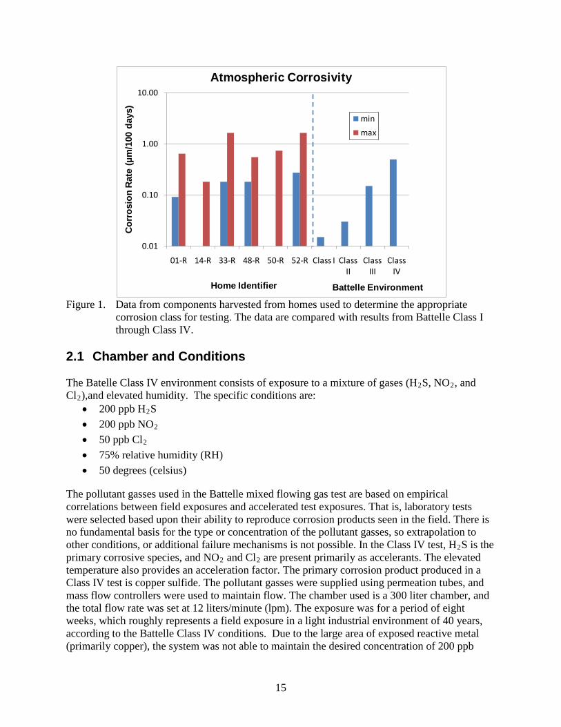
FIGURES Figure 1. Data from components harvested from homes used to determine the appropriate

corrosion class for testing. The data are compared with results from Battelle Class I through Class IV. .............................................................................................15

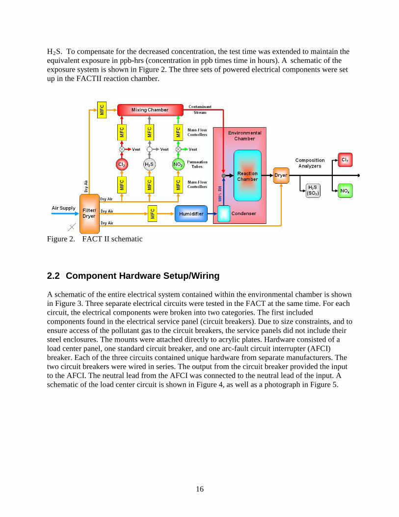
Figure 2. FACT II schematic .......................................................................................................16

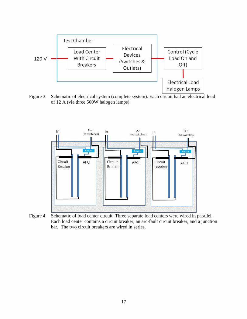
Figure 3. Schematic of electrical system (complete system). Each circuit had an electrical load of 12 A (via three 500W halogen lamps). ............................................................17

Figure 4. Schematic of load center circuit. Three separate load centers were wired in parallel. Each load center contains a circuit breaker, an arc-fault circuit breaker, and a junction bar. The two circuit breakers are wired in series.................................17

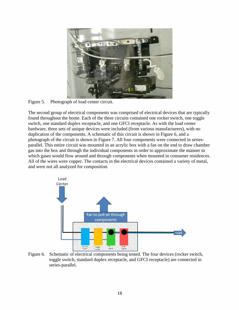
Figure 5. Photograph of load center circuit. ...............................................................................18

Figure 6. Schematic of electrical components being tested. The four devices (rocker switch, toggle switch, standard duplex receptacle, and GFCI receptacle) are connected in series-parallel. .........................................................................................18

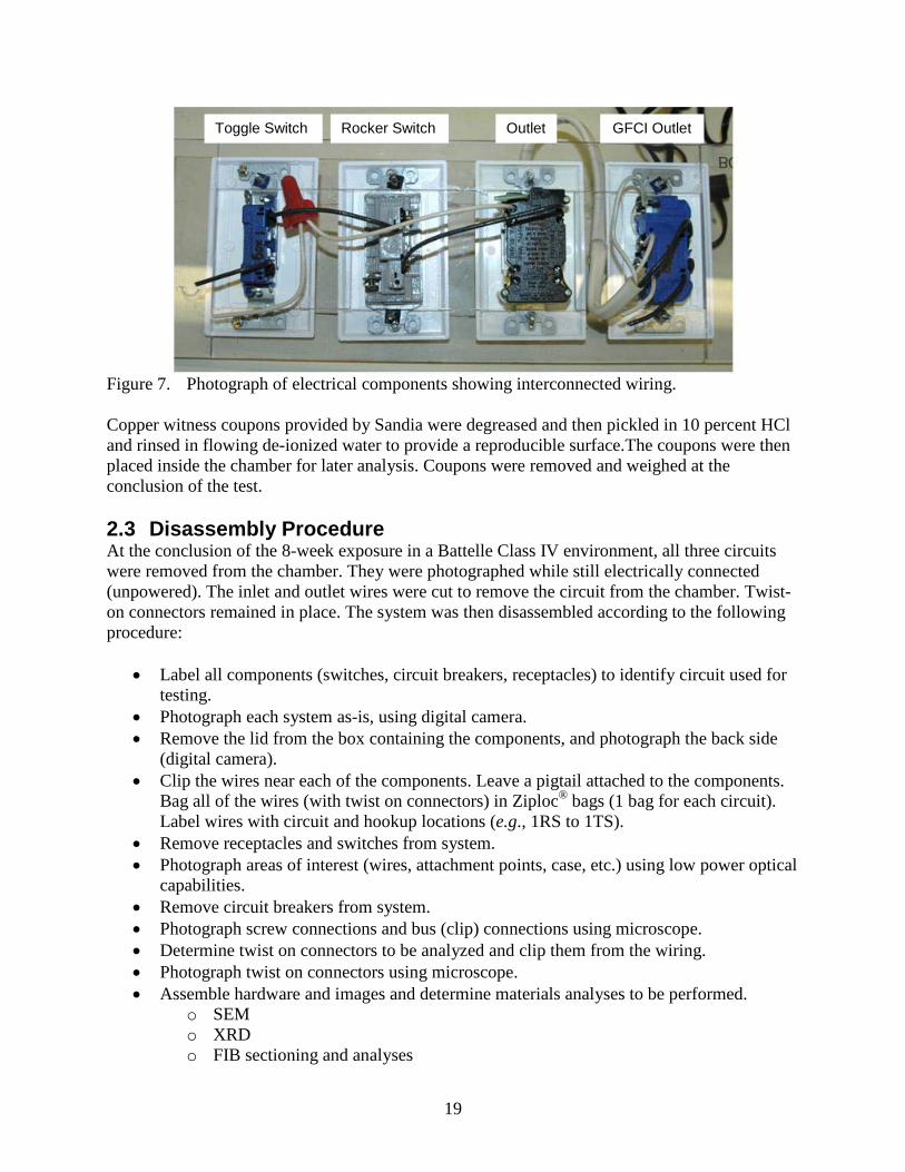
Figure 7. Photograph of electrical components showing interconnected wiring. .......................19

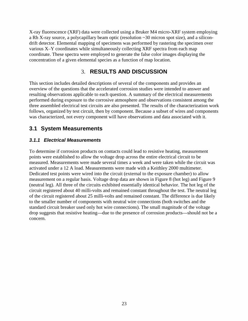
Figure 8. Voltage measurements made along the length of the ungrounded conductor (hot leg) for each of the three circuits, which included the load center and all the electrical components...................................................................................................24

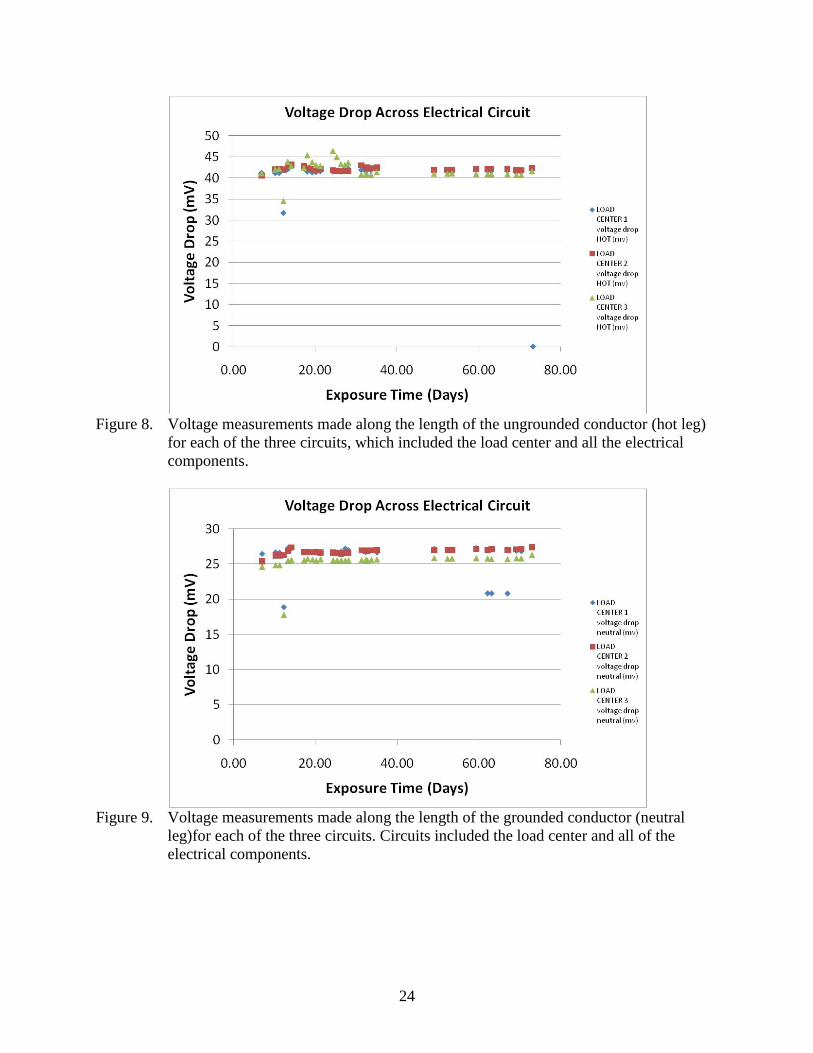
Figure 9. Voltage measurements made along the length of the grounded conductor (neutral leg)for each of the three circuits. Circuits included the load center and all of the electrical components. ..................................................................................24

Figure 10. Photographs of the electrical components tested in Circuit 1. The view from the bottom (C) shows how the system was wired electrically. ..........................................28

Figure 11. Optical images from sample 1-RS (rocker switch). The contact plate is shown in B, and one of the hot wires is shown in D (both sides of the same wire are shown). Note the presence of extensive corrosion product on the copper hot wire and contact plate. .................................................................................................30

Figure 12. SEM cross section of the hot screw plate (HSP2) from the rocker switch in Circuit No. 1.................................................................................................................31

Figure 13. SEM image (top left) and elemental maps using EDS of HSP2: sulfur (green), Cu (red), and Zn (purple). ............................................................................................31

Figure 14. Elemental maps using EDS of HSP2, showing chloride (yellow), and oxygen (blue). ...........................................................................................................................32

Figure 15. Photographs of toggle switch from Circuit 1. ..............................................................32

Figure 16. Photos of outside of GFCI receptacle from Circuit 1. .................................................33

Figure 17. Photos of inside of GFCI receptacle from Circuit 1. ..................................................34

Figure 18. SEM images of cross section of neutral wire 1-GR-NW1. .........................................35

7

Figure 19. Optical photographs of receptacle from Circuit 1. The image in (A) shows the side view of hot wires; (B) hot screw and contact plate; (C) side view of neutral wires; and (D) neutral screw and contact plate. ...........................................................36

Figure 20. Optical photographs of hot wire removed from receptacle from Circuit 1. .................36

Figure 21. SEM image (A) of hot wire 1-R-HW1; (B) SEM image of screw contact surface with zoomed area (top right); (C) EDS elemental map showing copper (red) and sulfur (green) distribution; and (D) SEM image ~300 µm from contact (all with 100 µm measurement bars). .........................................................................................37

Figure 22. SEM images showing the different morphologies of corrosion products on the hot wire from the receptacle in Circuit 1. ....................................................................38

Figure 23. SEM images and elemental maps for two areas on wire 1-R-HW-1, showing copper (red), oxygen (blue), carbon (purple), and sulfur (green) distributions. ..........39

Figure 24. Optical images of the load center and AFCI for Circuit 1. ..........................................40

Figure 25. SEM image of the cross section of the neutral wire from the arc-fault circuit breaker from Circuit 1. .................................................................................................41

Figure 26. EDS map of wire cross section showing oxygen in “pocket. The elemental maps for Cu (red), S (green), and oxygen (blue) are shown. .......................................42

Figure 27. Elemental maps taken on cross section of the neutral wire from the arc-fault circuit breaker from Circuit 1. The image at the top left is an SEM image of the area being analyzed. The elemental maps for Cu (red), S (green), and oxygen (blue) are shown. ..........................................................................................................43

Figure 28. Elemental maps taken on cross section of the neutral wire from the arc-fault circuit breaker from Circuit 1. The image on the left is an SEM image of the area being analyzed. The elemental maps for Cu (red), S (green), and oxygen (blue) are shown. ..........................................................................................................44

Figure 29. Optical images of the contacts in the standard circuit breaker in Circuit 1. ................45

Figure 30. Optical images of the plug used to connect the standard receptacle to the GFCI receptacle in Circuit 1. The prongs and screws are blackened relative to those on a new, as-received, unexposed plug. .......................................................................46

Figure 31. µ-XRD data for ground prong of plug from Circuit 1, showing cuprite (blue), covellite (green), and copper/zinc (orange) peaks observed and labels where digenite (D) peaks would occur, if present. .................................................................47

Figure 32. Photo of one side of ground prong and XRF element maps of ground prong of grounded plug. XRF images taken “end-on” of full prong. .........................................48

Figure 33. Video image (inset) showing location of µXRD analysis and µXRD data for witness coupon No. 5, showing labeled copper and djurleite peaks (green). ..............49

Figure 34. Photographs of the electrical components tested in Circuit 2. The view from the bottom (left image) shows how the system was wired electrically. The image on the right shows the load center. ....................................................................50

8

Figure 35. Optical images of wires from the rocker switch in Circuit 2. Both the standard wire connection and the push-in connection are shown. .............................................51

Figure 36. SEM images of the cross section of the rocker switch hot wire from Circuit 2. The image on the left shows a low magnification image of the wire, with a high magnification image showing details of the corrosion product layer presented in the figure on the right. ..................................................................................................51

Figure 37. Elemental maps from the rocker switch hot wire (cross sections) in Circuit 2. The upper left image is an SEM image identifying the area being analyzed. Three maps are shown for Cu (red), S (green), and oxygen (blue). ............................52

Figure 38. Video image (inset) and µ-XRD data for 2-RS-HSP-2 (contact plate), showing cuprite (orange), covellite (green), and copper/zinc (purple), and chalcocyanite (Cu+2SO4 53- light blue) peaks observed. .......................................................................

Figure 39. XRD data (top) for powder scraped from wire 2-R-GR-GW showing covelite (green) and antlerite (blue), and µ-XRD data (bottom) showing antlerite (orange), cuprite (light blue), covellite (dark blue), and copper (green) peaks. ..........54

Figure 40. Optical images of the rocker switch and hot wires from Circuit 3. .............................56

Figure 41. SEM images of the hot wire from the rocker switch in Circuit 3. The figures on the left are secondary electron images, which show topography. The images on the right are back-scatter images. In these images, brightness is a function of the atomic number, with higher brightness indicating elements of higher atomic number. ........................................................................................................................57

Figure 42. EDS elemental maps of the hot wire from the rocker switch in Circuit 3. Images include A the SEM image, (B) a copper map (red), (C) a sulfur map (green), and (D) a combined copper/sulfur map (red and green). .............................................58

Figure 43. Optical images of the toggle switch in Circuit 3. The figure on the left shows the inside of the switch. Note the extensive corrosion product on some of the components. The image on the right is of the hot wire connected to the toggle switch (screw side). ......................................................................................................59

Figure 44. SEM images of the hot wire from the toggle switch in Circuit 3. Note the spalling of the corrosion product film. The contact areas can be seen in the upper two images (bright areas) where the contact shielded the surface from the corrosive gasses. ..........................................................................................................59

Figure 45. SEM images and EDS elemental maps of the hot wire from the toggle switch in Circuit 3. Sulfur is shown in green, and copper is shown in red. ................................60

Figure 46. Low magnification FIB image of hot wire from toggle switch (3TS-HW-1), showing location of FIB cuts (red designated as “Section 1” and blue designated as “Section 2”) into corrosion product film. ..............................................61

Figure 47. FIB cuts into 3-TS-HW-1 “Section 1” (see Figure 46) with scale bars at 200 (350X), 50, 20, 5, and 5 (12,000X) microns, respectively. .........................................62

Figure 48. FIB cuts into 3-TS-HW-1 “Section 1” (see Figure 46) with scale bars at 4 microns each. ...............................................................................................................62

9

Figure 49. FIB cuts into 3-TS-HW-1 “Section 2” (see Figure 46) with scale bars at 50, 30, and 10 microns, respectively........................................................................................63

Figure 50. FIB cuts into hot wire from Circuit 3 toggle switch (3-TS-HW-1) “Section 2” (see Figure 46) with scale bars at 200, 50, 20, 10, 5, and 5 microns, respectively. .................................................................................................................63

Figure 51. FIB cuts into 3-TS-HW-1 “Section 2” (see Figure 46) with scale bars at 4 microns each (20,000X). ..............................................................................................64

Figure 52. Optical images of the GFCI receptacle. Note the darkening of the normally shiny contact pads and slight corrosion (discoloration) of the screws.........................64

Figure 53. Optical images of wires from the standard receptacle from Circuit 3. Both the (A) hot and (B) neutral wire are shown. Both are “push-in” type contacts. ................65

Figure 54. SEM images of the surface of the neutral wire from the receptacle in Circuit 3. The connection was a push-in connection. (B) shows the contact point, which is brighter due to the presence of Cu without S. The end of the wire is shown in the lower images at two magnifications. Note the spalling of the corrosion product film. It is believed that the spalling occurred during the test, but is it possible that it occurred after exposure and prior to analysis. .....................................66

Figure 55. FIB cuts into corrosion product on surface of neutral wire 3-R-PINW-1 with “Section 3” (left) and “Section 4” (right) with scale bar of 500 micron. .....................67

Figure 56. FIB cuts into neutral wire 3-R-PINW-1 “Section 3” (see Figure 55) with scale bars of 200, 50, 20, 10, 5, and 5 microns. ....................................................................68

Figure 57. FIB cuts into neutral wire 3-R-PINW-1 “Section 3” (see Figure 55) with scale bars of 4 micron each. ..................................................................................................68

Figure 58. FIB cuts into neutral wire 3-R-PINW-1 “Section 4” (see Figure 55) with scale bars of 200, 50, 20, 10, 5, and 3 microns, respectively................................................69

Figure 59. SEM images of the hot wire from the receptacle in Circuit 3. The connection was a push-in connection. The contact point is shown in the image on the left. The image on the right shows a region of a hot wire that was covered by insulation on the bottom...............................................................................................70

Figure 60. EDS elemental maps of the wire shown in Figure 59. Copper (red), sulfur (green), and oxygen (blue) are shown..........................................................................71

Figure 61. Optical images of twist-on connectors with hot and neutral wires used on the output section of Circuit 2............................................................................................72

10

TABLES

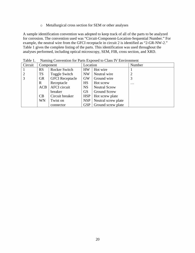
Table 1. Naming Convention for Parts Exposed to Class IV Environment ................................20

Table 2. Table of Corrosion Product Thickness Observed in SEM Cross Sections of Bare Copper Wires. ................................................................................................................27

Table 3. Table of Corrosion Product Thickness Observed in SEM Cross Sections of Brass Contact Pad HSP2. ........................................................................................................27

Table 4. Circuit No. 1 Components Submitted for Analysis .......................................................29

Table 5. Circuit No. 2 Components Submitted for Analysis. ......................................................50

Table 6. Circuit No. 3 Components Submitted for Analysis .......................................................55

Table 7. Table of Corrosion Ratings for Electrical Components from Homes. ..........................75

11

NOMENCLATURE AES Auger–Electron Spectroscopy AFCI arc-fault circuit interrupter Al aluminum Au gold CPSC Consumer Product Safety Commission Cr chromium ct contact tab Cu copper Cu2CuS covellite

O cuprite, copper oxide

CuSO4 Cu

chalcocyanite 3(SO4)(OH)4

Cu antlerite

9S5(Cu,Zn)

digenite, copper sulfide 5(SO4)6.6(H2

EDS energy dispersive spectroscopy O) ktenasite

FACT Facility for Atmospheric Corrosion Testing Fe iron FIB focused ion beam GFCI ground fault circuit interrupter GS ground screw GW ground wire HSP hot screw plate HS hot screw HW hot wire l left lpm liters per minute lcp left contact plate MFG mixed flowing gas m/z mass to charge ratio (in mass spectrometry) micrometer 1 millionth of a meter or 1x10-6

micron (µm) 1 millionth of a meter or 1x10 meters

-6

mm millimeter meters

m-ohm milli-ohm or one thousandth of an ohm Ni nickel NS neutral screw O oxygen PIHW push-in hot wire ppb parts per billion ppm parts per million Pt platinum R receptacle r right rcp right contact plate S sulfur

12

SEM scanning electron microscopy SNL Sandia National Laboratories Ti titanium XRD X-ray Diffraction XRF X-ray Fluorescence Z atomic number of element from the periodic table (e.g., Z for copper is 29) Zn zinc

13

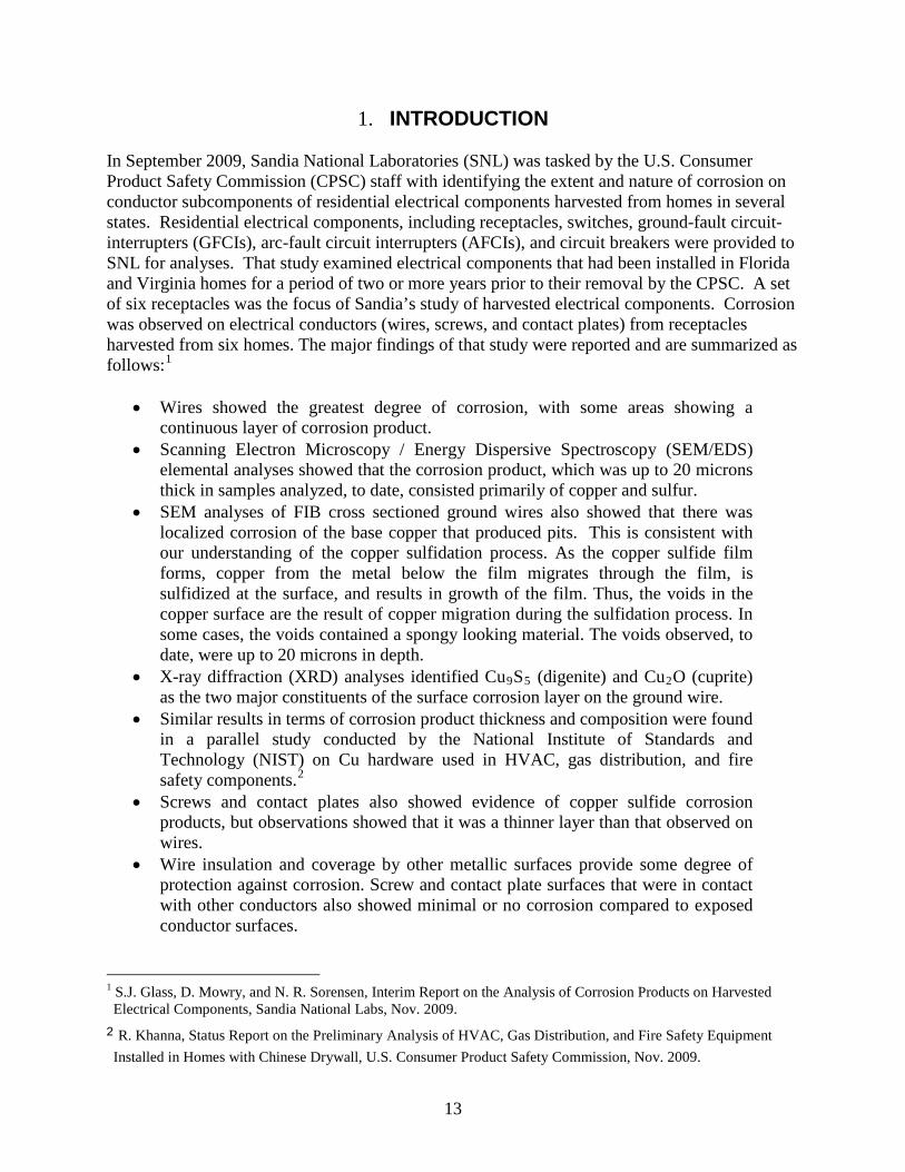
1. INTRODUCTION In September 2009, Sandia National Laboratories (SNL) was tasked by the U.S. Consumer Product Safety Commission (CPSC) staff with identifying the extent and nature of corrosion on conductor subcomponents of residential electrical components harvested from homes in several states. Residential electrical components, including receptacles, switches, ground-fault circuit-interrupters (GFCIs), arc-fault circuit interrupters (AFCIs), and circuit breakers were provided to SNL for analyses. That study examined electrical components that had been installed in Florida and Virginia homes for a period of two or more years prior to their removal by the CPSC. A set of six receptacles was the focus of Sandia’s study of harvested electrical components. Corrosion was observed on electrical conductors (wires, screws, and contact plates) from receptacles harvested from six homes. The major findings of that study were reported and are summarized as follows:1

• Wires showed the greatest degree of corrosion, with some areas showing a continuous layer of corrosion product.

• Scanning Electron Microscopy / Energy Dispersive Spectroscopy (SEM/EDS) elemental analyses showed that the corrosion product, which was up to 20 microns thick in samples analyzed, to date, consisted primarily of copper and sulfur.

• SEM analyses of FIB cross sectioned ground wires also showed that there was localized corrosion of the base copper that produced pits. This is consistent with our understanding of the copper sulfidation process. As the copper sulfide film forms, copper from the metal below the film migrates through the film, is sulfidized at the surface, and results in growth of the film. Thus, the voids in the copper surface are the result of copper migration during the sulfidation process. In some cases, the voids contained a spongy looking material. The voids observed, to date, were up to 20 microns in depth.

• X-ray diffraction (XRD) analyses identified Cu9S5 (digenite) and Cu2

• Similar results in terms of corrosion product thickness and composition were found in a parallel study conducted by the National Institute of Standards and Technology (NIST) on Cu hardware used in HVAC, gas distribution, and fire safety components.

O (cuprite) as the two major constituents of the surface corrosion layer on the ground wire.

2

• Screws and contact plates also showed evidence of copper sulfide corrosion products, but observations showed that it was a thinner layer than that observed on wires.

• Wire insulation and coverage by other metallic surfaces provide some degree of protection against corrosion. Screw and contact plate surfaces that were in contact with other conductors also showed minimal or no corrosion compared to exposed conductor surfaces.

1 S.J. Glass, D. Mowry, and N. R. Sorensen, Interim Report on the Analysis of Corrosion Products on Harvested Electrical Components, Sandia National Labs, Nov. 2009.

2 R. Khanna, Status Report on the Preliminary Analysis of HVAC, Gas Distribution, and Fire Safety Equipment Installed in Homes with Chinese Drywall, U.S. Consumer Product Safety Commission, Nov. 2009.

14

The 2009 study was able to identify the nature and extent of the corrosion product that had occurred during the exposure to problem drywall in the six homes, but not how much corrosion could occur for the typical lifetime of household electrical components, and what effects this might have on the electrical function and safety of powered circuits. To answer these questions, SNL designed and conducted the experimental study described in this report, in which new electrical components, supplied by CPSC, were exposed to elevated temperature and humidity, and contaminant gasses, including H2S, NO2, and Cl2, in Sandia’s larger Facility for Atmospheric Corrosion Testing or FACTII. The conditions of the test and the duration of the exposure were chosen to be representative of a Battelle Class IV3

environment to stimulate the growth of corrosion product that would be expected to be generated by a 40-year exposure to the conditions that produced the corrosion product thickness measured on harvested components in the 2009 study.

Three powered electrical circuits, consisting of switches, receptacles (conventional and GFCI), and load centers were cycled electrically over the 8-week exposure in the FACTII environmentally controlled chamber. The total cycle time was 20 minutes, with 10 minutes on, followed by 10 minutes off. The purpose of the cycling was to provide thermally-driven stresses of the corrosion product (due to differences in the thermal expansion properties of the metal conductors and the corrosion products). Furthermore, assessment of corrosion-induced functional impacts was performed while components were undergoing exposure. At the end of the exposure, the electrical components were subjected to the same materials analyses used for the characterization of harvested electrical components from the 2009 study, including SEM, XRD, and focused ion beam (FIB). These analyses were used to determine the morphology, thickness, and chemical identity of the observed corrosion layers.

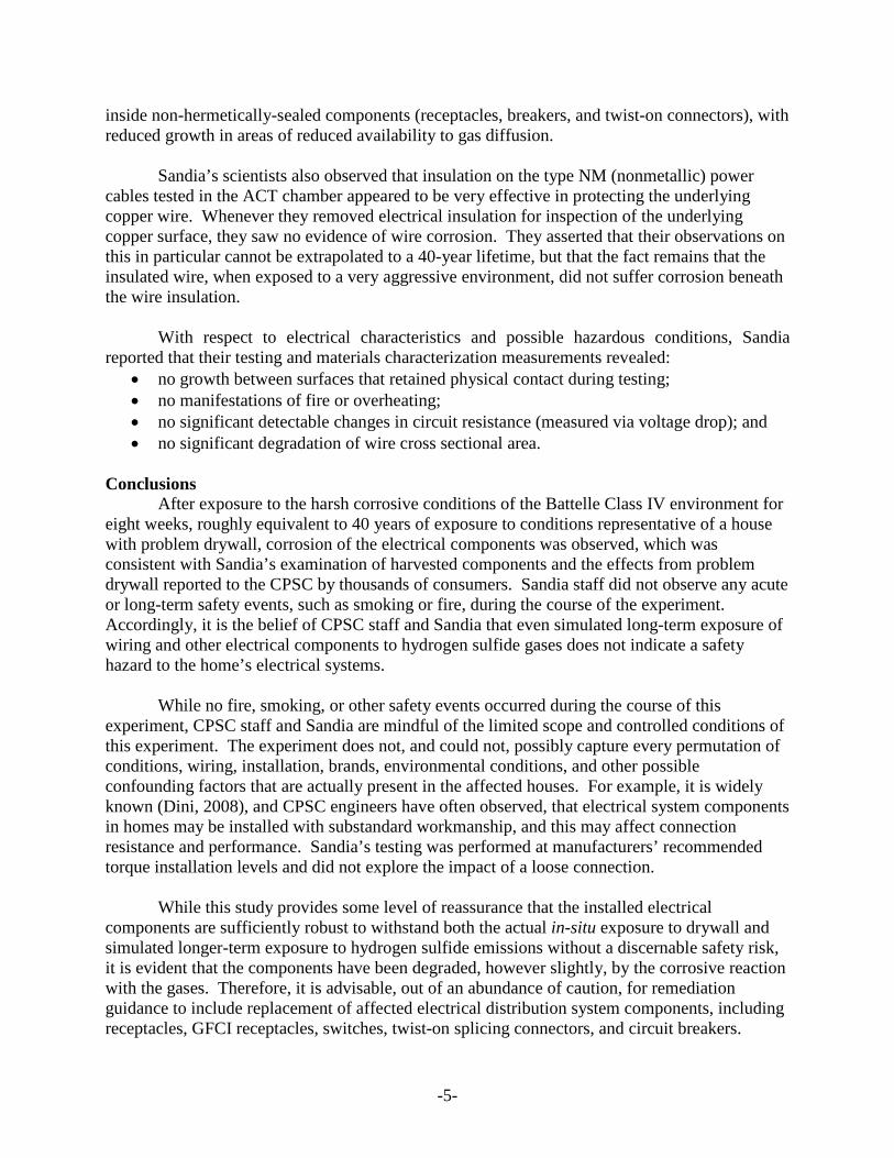
2. EXPERIMENTAL DETAILS This experiment was designed to test multiple components of a powered electrical system in an environmental chamber in which Battelle Class IV conditions were maintained. The selection of the Class IV environment was based on results from components harvested from several homes. The components were analyzed, and a corrosion product thickness was determined. The exposure was estimated to be three years. Figure 1 presents the data from the harvested components and compares the result to published mixed flowing gas testing. Based on these data, the best fit corrosion class appears to be Class IV, the most extreme corrosive conditions of the Battelle exposure system.

3 W. H. Abbott, The Development and Performance Characteristics of Mixed Flowing Gas Test Environment, IEEE Transactions, Vol. 11, No. 1, March 1988.

15

Figure 1. Data from components harvested from homes used to determine the appropriate

corrosion class for testing. The data are compared with results from Battelle Class I through Class IV.

2.1 Chamber and Conditions The Batelle Class IV environment consists of exposure to a mixture of gases (H2S, NO2, and Cl2

• 200 ppb H),and elevated humidity. The specific conditions are:

2

• 200 ppb NOS

• 50 ppb Cl2

• 75% relative humidity (RH) 2

• 50 degrees (celsius)

The pollutant gasses used in the Battelle mixed flowing gas test are based on empirical correlations between field exposures and accelerated test exposures. That is, laboratory tests were selected based upon their ability to reproduce corrosion products seen in the field. There is no fundamental basis for the type or concentration of the pollutant gasses, so extrapolation to other conditions, or additional failure mechanisms is not possible. In the Class IV test, H2S is the primary corrosive species, and NO2 and Cl2

0.01

0.10

1.00

10.00

01-R 14-R 33-R 48-R 50-R 52-R Class I Class II

Class III

Class IV

Cor

rosi

on R

ate

(µm

/100

day

s)

Home Identifier

Atmospheric Corrosivity

min

max

Battelle Environment

are present primarily as accelerants. The elevated temperature also provides an acceleration factor. The primary corrosion product produced in a Class IV test is copper sulfide. The pollutant gasses were supplied using permeation tubes, and mass flow controllers were used to maintain flow. The chamber used is a 300 liter chamber, and the total flow rate was set at 12 liters/minute (lpm). The exposure was for a period of eight weeks, which roughly represents a field exposure in a light industrial environment of 40 years, according to the Battelle Class IV conditions. Due to the large area of exposed reactive metal (primarily copper), the system was not able to maintain the desired concentration of 200 ppb

16

H2

Figure 2

S. To compensate for the decreased concentration, the test time was extended to maintain the equivalent exposure in ppb-hrs (concentration in ppb times time in hours). A schematic of the exposure system is shown in . The three sets of powered electrical components were set up in the FACTII reaction chamber.

Figure 2. FACT II schematic 2.2 Component Hardware Setup/Wiring A schematic of the entire electrical system contained within the environmental chamber is shown in Figure 3. Three separate electrical circuits were tested in the FACT at the same time. For each circuit, the electrical components were broken into two categories. The first included components found in the electrical service panel (circuit breakers). Due to size constraints, and to ensure access of the pollutant gas to the circuit breakers, the service panels did not include their steel enclosures. The mounts were attached directly to acrylic plates. Hardware consisted of a load center panel, one standard circuit breaker, and one arc-fault circuit interrupter (AFCI) breaker. Each of the three circuits contained unique hardware from separate manufacturers. The two circuit breakers were wired in series. The output from the circuit breaker provided the input to the AFCI. The neutral lead from the AFCI was connected to the neutral lead of the input. A schematic of the load center circuit is shown in Figure 4, as well as a photograph in Figure 5.

17

Figure 3. Schematic of electrical system (complete system). Each circuit had an electrical load

of 12 A (via three 500W halogen lamps).

Figure 4. Schematic of load center circuit. Three separate load centers were wired in parallel.

Each load center contains a circuit breaker, an arc-fault circuit breaker, and a junction bar. The two circuit breakers are wired in series.

120 V

18

Figure 5. Photograph of load center circuit. The second group of electrical components was comprised of electrical devices that are typically found throughout the home. Each of the three circuits contained one rocker switch, one toggle switch, one standard duplex receptacle, and one GFCI receptacle. As with the load center hardware, three sets of unique devices were included (from various manufacturers), with no duplication of the components. A schematic of this circuit is shown in Figure 6, and a photograph of the circuit is shown in Figure 7. All four components were connected in series-parallel. This entire circuit was mounted in an acrylic box with a fan on the end to draw chamber gas into the box and through the individual components in order to approximate the manner in which gases would flow around and through components when mounted in consumer residences. All of the wires were copper. The contacts in the electrical devices contained a variety of metal, and were not all analyzed for composition.

Figure 6. Schematic of electrical components being tested. The four devices (rocker switch,

toggle switch, standard duplex receptacle, and GFCI receptacle) are connected in series-parallel.

19

Figure 7. Photograph of electrical components showing interconnected wiring. Copper witness coupons provided by Sandia were degreased and then pickled in 10 percent HCl and rinsed in flowing de-ionized water to provide a reproducible surface.The coupons were then placed inside the chamber for later analysis. Coupons were removed and weighed at the conclusion of the test. 2.3 Disassembly Procedure At the conclusion of the 8-week exposure in a Battelle Class IV environment, all three circuits were removed from the chamber. They were photographed while still electrically connected (unpowered). The inlet and outlet wires were cut to remove the circuit from the chamber. Twist-on connectors remained in place. The system was then disassembled according to the following procedure:

• Label all components (switches, circuit breakers, receptacles) to identify circuit used for testing.

• Photograph each system as-is, using digital camera. • Remove the lid from the box containing the components, and photograph the back side

(digital camera). • Clip the wires near each of the components. Leave a pigtail attached to the components.

Bag all of the wires (with twist on connectors) in Ziploc®

• Remove receptacles and switches from system.

bags (1 bag for each circuit). Label wires with circuit and hookup locations (e.g., 1RS to 1TS).

• Photograph areas of interest (wires, attachment points, case, etc.) using low power optical capabilities.

• Remove circuit breakers from system. • Photograph screw connections and bus (clip) connections using microscope. • Determine twist on connectors to be analyzed and clip them from the wiring. • Photograph twist on connectors using microscope. • Assemble hardware and images and determine materials analyses to be performed.

o SEM o XRD o FIB sectioning and analyses

Toggle Switch

Rocker Switch

Outlet

GFCI Outlet

20

o Metallurgical cross section for SEM or other analyses A sample identification convention was adopted to keep track of all of the parts to be analyzed for corrosion. The convention used was “Circuit-Component-Location-Sequential Number.” For example, the neutral wire from the GFCI receptacle in circuit 2 is identified as “2-GR-NW-2.” Table 1 gives the complete listing of the parts. This identification was used throughout the analyses performed, including optical microscopy, SEM, FIB, cross section, and XRD. Table 1. Naming Convention for Parts Exposed to Class IV Environment Circuit Component Location Number 1 2 3

RS TS GR R ACB CB WN

Rocker Switch Toggle Switch GFCI Receptacle Receptacle AFCI circuit breaker Circuit breaker Twist on connector

HW NW GW HS NS GS HSP NSP GSP

Hot wire Neutral wire Ground wire Hot screw Neutral Screw Ground Screw Hot screw plate Neutral screw plate Ground screw plate

1 2 3 …

21

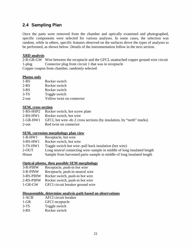
2.4 Sampling Plan Once the parts were removed from the chamber and optically examined and photographed, specific components were selected for various analyses. In some cases, the selection was random, while in others, specific features observed on the surfaces drove the types of analyses to be performed, as shown below. Details of the instrumentation follow in the next section.

2-R-GR-GW Wire between the receptacle and the GFCI, unattached copper ground wire circuit XRD analysis

1-plug Connector plug from circuit 1 that was in receptacle Copper coupon from chamber, randomly selected

1-RS Rocker switch Photos only

2-RS Rocker switch 3-RS Rocker switch 3-TS Toggle switch 2-out Yellow twist on connector

1-RS-HSP2 Rocker switch, hot screw plate SEM, cross section

2-RS-HW1 Rocker switch, hot wire 1-GR-HW1 GFCI, hot wire–do 2 cross sections (by insulation, by “teeth” marks) 2-out Red twist on connector

1-R-HW1 Receptacle, hot wire SEM, corrosion morphology plan view

3-RS-HW1 Rocker switch, hot wire 3-TS-HW1 Toggle switch hot wire–pull back insulation (hot wire) 2-OUT Long neutral connecting wire–sample in middle of long insulated length House Sample from harvested parts–sample in middle of long insulated length

3-R-PIHW Receptacle, push-in hot wire Optical photos, then possible SEM morphology

3-R-PINW Receptacle, push-in neutral wire 3-RS-PIHW Rocker switch, push-in hot wire 2-RS-PIHW Rocker switch, push-in hot wire 1-GR-GW GFCI circuit breaker ground wire

1-ACB AFCI circuit breaker Dissassemble, determine analysis path based on observations

1-GR GFCI receptacle 3-TS Toggle switch 3-RS Rocker switch

22

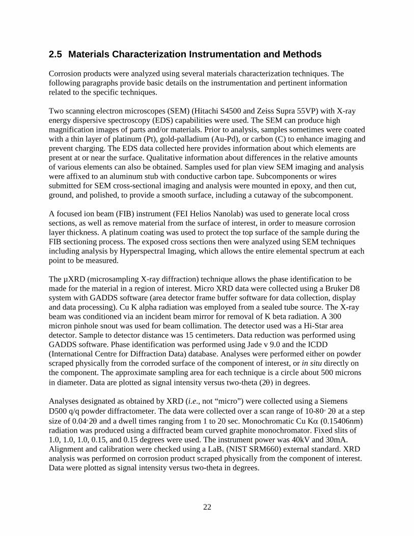
2.5 Materials Characterization Instrumentation and Methods Corrosion products were analyzed using several materials characterization techniques. The following paragraphs provide basic details on the instrumentation and pertinent information related to the specific techniques. Two scanning electron microscopes (SEM) (Hitachi S4500 and Zeiss Supra 55VP) with X-ray energy dispersive spectroscopy (EDS) capabilities were used. The SEM can produce high magnification images of parts and/or materials. Prior to analysis, samples sometimes were coated with a thin layer of platinum (Pt), gold-palladium (Au-Pd), or carbon (C) to enhance imaging and prevent charging. The EDS data collected here provides information about which elements are present at or near the surface. Qualitative information about differences in the relative amounts of various elements can also be obtained. Samples used for plan view SEM imaging and analysis were affixed to an aluminum stub with conductive carbon tape. Subcomponents or wires submitted for SEM cross-sectional imaging and analysis were mounted in epoxy, and then cut, ground, and polished, to provide a smooth surface, including a cutaway of the subcomponent. A focused ion beam (FIB) instrument (FEI Helios Nanolab) was used to generate local cross sections, as well as remove material from the surface of interest, in order to measure corrosion layer thickness. A platinum coating was used to protect the top surface of the sample during the FIB sectioning process. The exposed cross sections then were analyzed using SEM techniques including analysis by Hyperspectral Imaging, which allows the entire elemental spectrum at each point to be measured. The µXRD (microsampling X-ray diffraction) technique allows the phase identification to be made for the material in a region of interest. Micro XRD data were collected using a Bruker D8 system with GADDS software (area detector frame buffer software for data collection, display and data processing). Cu K alpha radiation was employed from a sealed tube source. The X-ray beam was conditioned via an incident beam mirror for removal of K beta radiation. A 300 micron pinhole snout was used for beam collimation. The detector used was a Hi-Star area detector. Sample to detector distance was 15 centimeters. Data reduction was performed using GADDS software. Phase identification was performed using Jade v 9.0 and the ICDD (International Centre for Diffraction Data) database. Analyses were performed either on powder scraped physically from the corroded surface of the component of interest, or in situ directly on the component. The approximate sampling area for each technique is a circle about 500 microns in diameter. Data are plotted as signal intensity versus two-theta (2θ) in degrees. Analyses designated as obtained by XRD (i.e., not “micro”) were collected using a Siemens D500 q/q powder diffractometer. The data were collected over a scan range of 10-80ο 2θ at a step size of 0.04o 2θ and a dwell times ranging from 1 to 20 sec. Monochromatic Cu Kα (0.15406nm) radiation was produced using a diffracted beam curved graphite monochromator. Fixed slits of 1.0, 1.0, 1.0, 0.15, and 0.15 degrees were used. The instrument power was 40kV and 30mA. Alignment and calibration were checked using a LaB6

(NIST SRM660) external standard. XRD analysis was performed on corrosion product scraped physically from the component of interest. Data were plotted as signal intensity versus two-theta in degrees.

23

X-ray fluorescence (XRF) data were collected using a Bruker M4 micro-XRF system employing a Rh X-ray source, a polycapillary beam optic (resolution ~30 micron spot size), and a silicon-drift detector. Elemental mapping of specimens was performed by rastering the specimen over various X–Y coordinates while simultaneously collecting XRF spectra from each map coordinate. These spectra were employed to generate the false color images displaying the concentration of a given elemental species as a function of map location.

3. RESULTS AND DISCUSSION This section includes detailed descriptions of several of the components and provides an overview of the questions that the accelerated corrosion studies were intended to answer and resulting observations applicable to each question. A summary of the electrical measurements performed during exposure to the corrosive atmosphere and observations consistent among the three assembled electrical test circuits are also presented. The results of the characterization work follows, organized by test circuit, then by component. Because a subset of wires and components was characterized, not every component will have observations and data associated with it. 3.1 System Measurements 3.1.1 Electrical Measurements To determine if corrosion products on contacts could lead to resistive heating, measurement points were established to allow the voltage drop across the entire electrical circuit to be measured. Measurements were made several times a week and were taken while the circuit was activated under a 12 A load. Measurements were made with a Keithley 2000 multimeter. Dedicated test points were wired into the circuit (external to the exposure chamber) to allow measurement on a regular basis. Voltage drop data are shown in Figure 8 (hot leg) and Figure 9 (neutral leg). All three of the circuits exhibited essentially identical behavior. The hot leg of the circuit registered about 40 milli-volts and remained constant throughout the test. The neutral leg of the circuit registered about 25 milli-volts and remained constant. The difference is due likely to the smaller number of components with neutral wire connections (both switches and the standard circuit breaker used only hot wire connections). The small magnitude of the voltage drop suggests that resistive heating—due to the presence of corrosion products—should not be a concern.

24

Figure 8. Voltage measurements made along the length of the ungrounded conductor (hot leg)

for each of the three circuits, which included the load center and all the electrical components.

Figure 9. Voltage measurements made along the length of the grounded conductor (neutral

leg)for each of the three circuits. Circuits included the load center and all of the electrical components.

25

3.2 Observations Across All Circuits Several materials characterization tests were performed on a variety of components to measure and observe the corrosion product across different metals and components. Following disassembly, all three circuits had the following similarities:

• Extensive black corrosion product on bare wires; • Variability in extent of corrosion (thicknesses, colors, morphology) on contact screws; • Lack of corrosion observed on galvanized metal plates; • A variety of microgrowth morphologies; • Apparent “layering” of growth; • Variations in corrosion product thickness between the inner (less gas access) and outer

(exposed) areas; • Flaking, blistering, and spalling of corrosion product films. This type of behavior is often

observed with thick corrosion product films on metal substrates. • Bare metal at contact points (pinch-points or screw contacts, contact plates) on wires,

screws, and contact plates; • Evidence of oxidation on the outer surface of the sulfide films. This is consistent with

long-time exposure in an oxidizing environment. • Multiple phases of copper sulfide on various surfaces.

Several of these observations have precedent in the literature of corroded copper, even though much of the literature is for tests with shorter timeframes and less aggressive conditions than those described in this report. These references illustrate the complexity observed in the products. For example, a variety of microgrowth morphologies have been observed in atmospheric monitoring of corrosion and controlled laboratory testing.4,5,6 Similar “layering” of growth has been observed using SEM and other analysis techniques.7,8 The flaking, blistering, and spalling of corrosion product films observed here is often observed with thick corrosion product films on metal substrates.4,8,9 The presence of multiple phases of copper sulfide, and in some cases, the oxidized form antlerite, also has precedent.6,7

4 T.T.M. Tran, C. Fiaud, E.M.M. Sutter, A. Villanova, The Atmospheric Corrosion of Copper by Hydrogen Sulphide in Underground Conditions, in Corros Sci, Vol. 45, pp. 2787-802, 2003.

In many studies, the goal did not

5J.C. Barbour, J.P. Sullivan, M.J. Campin, A.F. Wright, N.A. Missert, J.W. Braithwaite, K.R. Zavadil, N.R. Sorensen, S.J. Lucero, W. G. Breiland, and H.K. Moffat, Mechanisms of Atmospheric Copper Sulfidation and Evaluation of Parallel Experimentation Techniques, SAND2002-0699. Sandia National Laboratories, 2002.

6 M. Watanabe, Y. Higashi, T. Ichino, Surface Observation and Depth Profiling Analysis Studies of Corrosion Products on Copper Exposed Outdoors, in J Electrochem Soc, Vol. 150, pp. B37-B44, 2003.

7 M. Reid, J. Punch, L.F. Garfias-Mesias, K. Shannon, S. Belochapkine, D.A. Tanner, Study of Mixed Flowing Gas Exposure of Copper, in J Electrochem Soc, Vol. 155, pp. C147-C53, 2008.

8 K. Demirkan, G.E. Derkits, D.A. Fleming, J.P. Franey, K. Hannigan, R.L. Opila, J. Punch, W.D. Reents, M. Reid, B. Wright, C. Xu, Corrosion of Cu under Highly Corrosive Environments, in J Electrochem Soc, Vol. 157, pp. C30-C35, 2010.

9 M. Reid, J. Punch, C. Ryan, L.F. Garfias, S. Belochapkine, J.P. Franey, G.E. Derkits, W.D. Reents, Microstructural Development of Copper Sulfide on Copper Exposed to Humid H2S, in J Electrochem Soc, Vol. 154, pp. C209-C14, 2007.

26

include identifying a specific crystal phase or stoichiometry. Therefore, only a generic Cu2S assignment is made in these published reports.10

Some of the specific crystalline phases of copper sulfide observed here are different than the digenite phase observed in the harvested components reported earlier. This is not unexpected because the accelerated conditions used here were not meant to mimic exactly conditions in the field. The sulfidation corrosion of copper is a complex event in which electrochemical, chemical, thermodynamic, and diffusion processes are all occurring. Each process is dependent upon factors such as temperature, concentration of gases present, and composition of local material at the surface. For atmospheric corrosion, or corrosion in mixed flowing gas experiments such as those in which oxygen is present, both copper oxides and sulfides form. In the case of copper sulfides, a variety of crystalline phases (elemental arrangements), each with a different stoichiometry (ratio of copper to sulfur), is possible and also can be found in nature. Some natural minerals, their stoichiometries, and weight percent of copper, include chalcocite (Cu2S – 79.85% Cu), djurleite (Cu31S16–79.34% Cu), digenite (Cu9S5–78.10% Cu), and covellite (CuS–66.46% Cu). In nature, and in laboratory tests, these copper sulfides can be oxidized and/or hydrated to form additional species, such as antlerite (Cu3(SO4)(OH)4) and posnajakite (Cu4(SO4)(OH)6·H2

O). For these reasons, the specific phase detected is less important than where the corrosion is (or is not) occurring.

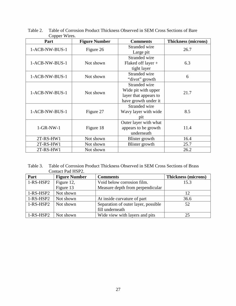
The following tables contain comparisons of corrosion product thicknesses, using measurements from SEM cross section images of bare copper wires and a brass contact pad (1-RS-HSP2). The Figure number in this table documents where some of the SEM images used for these measurements can be observed. These measurements are not meant as a statistical sampling, and in each case, the thickest area or interesting feature was selected for measurement. These thicknesses are greater than those observed in the harvested components reported previously, where the maximum thickness found in any of the homes analyzed was 18 microns.

10 T.T.M. Tran, C. Fiaud, E.M.M. Sutter, Oxide and Sulphide Layers on Copper Exposed to H2S Containing Moist

Air, in Corros Sci, Vol. 47, pp. 1724-37, 2005.

27

Table 2. Table of Corrosion Product Thickness Observed in SEM Cross Sections of Bare Copper Wires.

Part Figure Number Comments Thickness (microns)

1-ACB-NW-BUS-1 Figure 26 Stranded wire Large pit 26.7

1-ACB-NW-BUS-1 Not shown Stranded wire

Flaked off layer + tight layer

6.3

1-ACB-NW-BUS-1 Not shown Stranded wire “divot” growth 6

1-ACB-NW-BUS-1 Not shown

Stranded wire Wide pit with upper layer that appears to have growth under it

21.7

1-ACB-NW-BUS-1 Figure 27 Stranded wire

Wavy layer with wide pit

8.5

1-GR-NW-1 Figure 18 Outer layer with what appears to be growth

underneath 11.4

2T-RS-HW1 Not shown Blister growth 16.4 2T-RS-HW1 Not shown Blister growth 25.7 2T-RS-HW1 Not shown 26.2

Table 3. Table of Corrosion Product Thickness Observed in SEM Cross Sections of Brass

Contact Pad HSP2. Part Figure Number Comments Thickness (microns) 1-RS-HSP2 Figure 12,

Figure 13 Void below corrosion film. Measure depth from perpendicular

15.3

1-RS-HSP2 Not shown 12 1-RS-HSP2 Not shown At inside curvature of part 36.6 1-RS-HSP2 Not shown Separation of outer layer, possible

fill underneath 52

1-RS-HSP2 Not shown Wide view with layers and pits 25

28

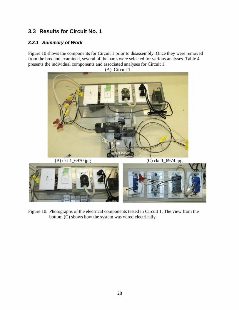
3.3 Results for Circuit No. 1 3.3.1 Summary of Work Figure 10 shows the components for Circuit 1 prior to disassembly. Once they were removed from the box and examined, several of the parts were selected for various analyses. Table 4 presents the individual components and associated analyses for Circuit 1.

(A) Circuit 1

(B) ckt-1_6970.jpg

(C) ckt-1_6974.jpg

Figure 10. Photographs of the electrical components tested in Circuit 1. The view from the bottom (C) shows how the system was wired electrically.

29

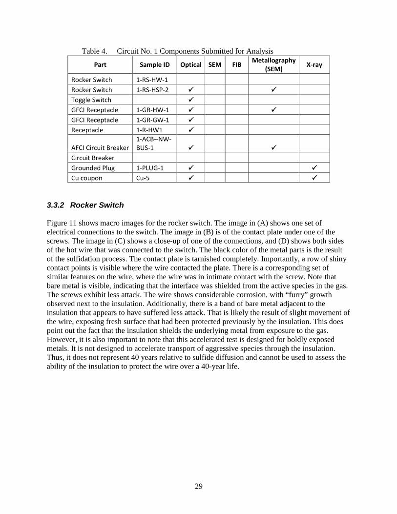
Table 4. Circuit No. 1 Components Submitted for Analysis

Part Sample ID Optical SEM FIB Metallography

(SEM) X-ray

Rocker Switch 1-RS-HW-1 Rocker Switch 1-RS-HSP-2 Toggle Switch GFCI Receptacle 1-GR-HW-1 GFCI Receptacle 1-GR-GW-1 Receptacle 1-R-HW1

AFCI Circuit Breaker 1-ACB--NW-BUS-1

Circuit Breaker Grounded Plug 1-PLUG-1 Cu coupon Cu-5

3.3.2 Rocker Switch Figure 11 shows macro images for the rocker switch. The image in (A) shows one set of electrical connections to the switch. The image in (B) is of the contact plate under one of the screws. The image in (C) shows a close-up of one of the connections, and (D) shows both sides of the hot wire that was connected to the switch. The black color of the metal parts is the result of the sulfidation process. The contact plate is tarnished completely. Importantly, a row of shiny contact points is visible where the wire contacted the plate. There is a corresponding set of similar features on the wire, where the wire was in intimate contact with the screw. Note that bare metal is visible, indicating that the interface was shielded from the active species in the gas. The screws exhibit less attack. The wire shows considerable corrosion, with “furry” growth observed next to the insulation. Additionally, there is a band of bare metal adjacent to the insulation that appears to have suffered less attack. That is likely the result of slight movement of the wire, exposing fresh surface that had been protected previously by the insulation. This does point out the fact that the insulation shields the underlying metal from exposure to the gas. However, it is also important to note that this accelerated test is designed for boldly exposed metals. It is not designed to accelerate transport of aggressive species through the insulation. Thus, it does not represent 40 years relative to sulfide diffusion and cannot be used to assess the ability of the insulation to protect the wire over a 40-year life.

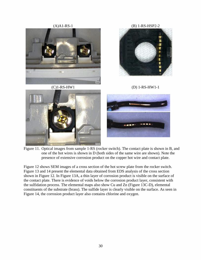
30

(A)A1-RS-1

(B) 1-RS-HSP2-2

(C)1-RS-HW1

(D) 1-RS-HW1-1

Figure 11. Optical images from sample 1-RS (rocker switch). The contact plate is shown in B, and one of the hot wires is shown in D (both sides of the same wire are shown). Note the presence of extensive corrosion product on the copper hot wire and contact plate.

Figure 12 shows SEM images of a cross section of the hot screw plate from the rocker switch. Figure 13 and 14 present the elemental data obtained from EDS analysis of the cross section shown in Figure 12. In Figure 13A, a thin layer of corrosion product is visible on the surface of the contact plate. There is evidence of voids below the corrosion product layer, consistent with the sulfidation process. The elemental maps also show Cu and Zn (Figure 13C-D), elemental constituents of the substrate (brass). The sulfide layer is clearly visible on the surface. As seen in Figure 14, the corrosion product layer also contains chlorine and oxygen.

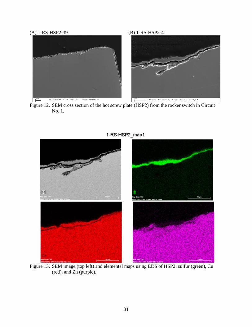
31

(A) 1-RS-HSP2-39

(B) 1-RS-HSP2-41

Figure 12. SEM cross section of the hot screw plate (HSP2) from the rocker switch in Circuit

No. 1.

Figure 13. SEM image (top left) and elemental maps using EDS of HSP2: sulfur (green), Cu

(red), and Zn (purple).

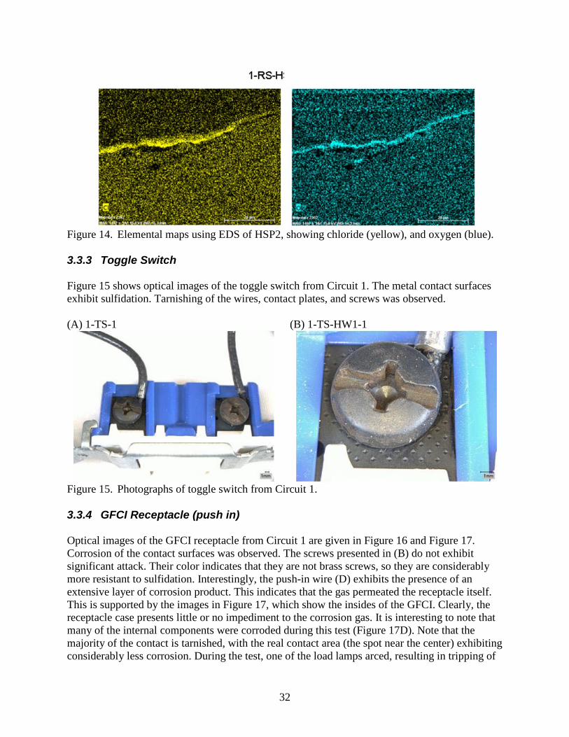
32

Figure 14. Elemental maps using EDS of HSP2, showing chloride (yellow), and oxygen (blue). 3.3.3 Toggle Switch Figure 15 shows optical images of the toggle switch from Circuit 1. The metal contact surfaces exhibit sulfidation. Tarnishing of the wires, contact plates, and screws was observed. (A) 1-TS-1

(B) 1-TS-HW1-1

Figure 15. Photographs of toggle switch from Circuit 1. 3.3.4 GFCI Receptacle (push in) Optical images of the GFCI receptacle from Circuit 1 are given in Figure 16 and Figure 17. Corrosion of the contact surfaces was observed. The screws presented in (B) do not exhibit significant attack. Their color indicates that they are not brass screws, so they are considerably more resistant to sulfidation. Interestingly, the push-in wire (D) exhibits the presence of an extensive layer of corrosion product. This indicates that the gas permeated the receptacle itself. This is supported by the images in Figure 17, which show the insides of the GFCI. Clearly, the receptacle case presents little or no impediment to the corrosion gas. It is interesting to note that many of the internal components were corroded during this test (Figure 17D). Note that the majority of the contact is tarnished, with the real contact area (the spot near the center) exhibiting considerably less corrosion. During the test, one of the load lamps arced, resulting in tripping of

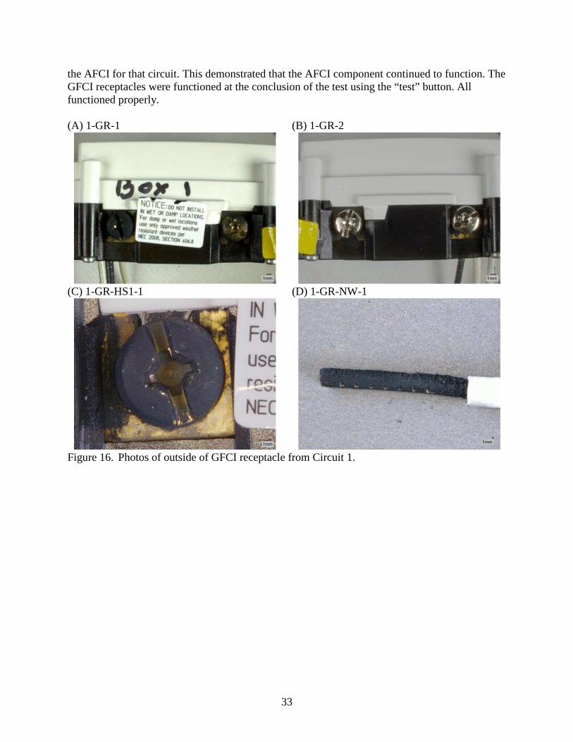
33

the AFCI for that circuit. This demonstrated that the AFCI component continued to function. The GFCI receptacles were functioned at the conclusion of the test using the “test” button. All functioned properly. (A) 1-GR-1

(B) 1-GR-2

(C) 1-GR-HS1-1

(D) 1-GR-NW-1

Figure 16. Photos of outside of GFCI receptacle from Circuit 1.

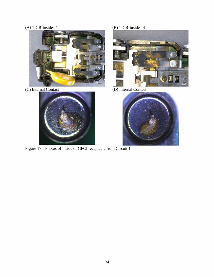
34

(A) 1-GR-insides-1

(B) 1-GR-insides-4

(C) Internal Contact

(D) Internal Contact

Figure 17. Photos of inside of GFCI receptacle from Circuit 1.

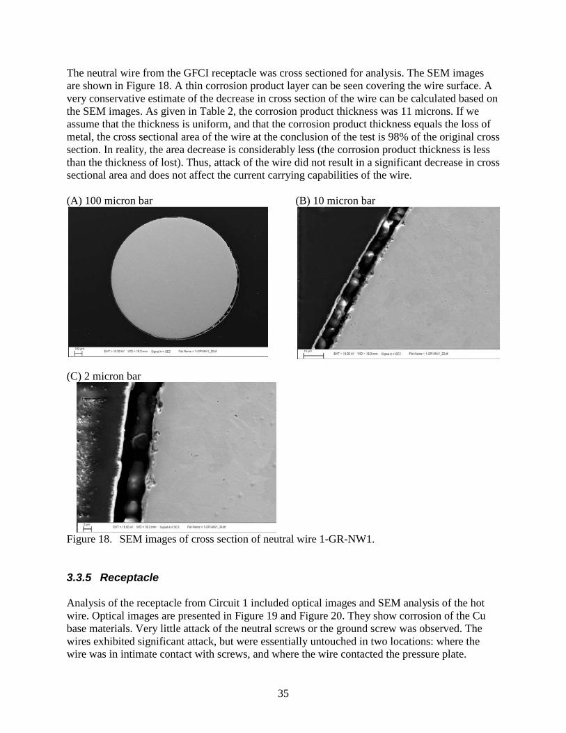
35

The neutral wire from the GFCI receptacle was cross sectioned for analysis. The SEM images are shown in Figure 18. A thin corrosion product layer can be seen covering the wire surface. A very conservative estimate of the decrease in cross section of the wire can be calculated based on the SEM images. As given in Table 2, the corrosion product thickness was 11 microns. If we assume that the thickness is uniform, and that the corrosion product thickness equals the loss of metal, the cross sectional area of the wire at the conclusion of the test is 98% of the original cross section. In reality, the area decrease is considerably less (the corrosion product thickness is less than the thickness of lost). Thus, attack of the wire did not result in a significant decrease in cross sectional area and does not affect the current carrying capabilities of the wire. (A) 100 micron bar

(B) 10 micron bar

(C) 2 micron bar

Figure 18. SEM images of cross section of neutral wire 1-GR-NW1. 3.3.5 Receptacle Analysis of the receptacle from Circuit 1 included optical images and SEM analysis of the hot wire. Optical images are presented in Figure 19 and Figure 20. They show corrosion of the Cu base materials. Very little attack of the neutral screws or the ground screw was observed. The wires exhibited significant attack, but were essentially untouched in two locations: where the wire was in intimate contact with screws, and where the wire contacted the pressure plate.

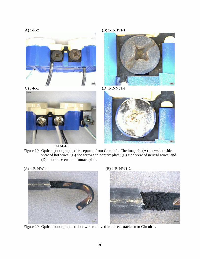
36

(A) 1-R-2

(B) 1-R-HS1-1

(C) 1-R-1

IMAGE

(D) 1-R-NS1-1

Figure 19. Optical photographs of receptacle from Circuit 1. The image in (A) shows the side view of hot wires; (B) hot screw and contact plate; (C) side view of neutral wires; and (D) neutral screw and contact plate.

(A) 1-R-HW1-1

(B) 1-R-HW1-2

Figure 20. Optical photographs of hot wire removed from receptacle from Circuit 1.

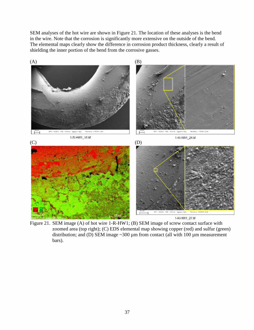
37

SEM analyses of the hot wire are shown in Figure 21. The location of these analyses is the bend in the wire. Note that the corrosion is significantly more extensive on the outside of the bend. The elemental maps clearly show the difference in corrosion product thickness, clearly a result of shielding the inner portion of the bend from the corrosive gasses. (A)

(B)

(C)

(D)

Figure 21. SEM image (A) of hot wire 1-R-HW1; (B) SEM image of screw contact surface with

zoomed area (top right); (C) EDS elemental map showing copper (red) and sulfur (green) distribution; and (D) SEM image ~300 µm from contact (all with 100 µm measurement bars).

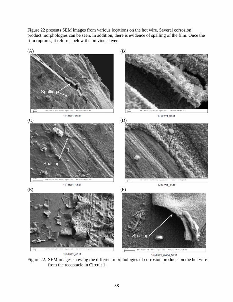
38

Figure 22 presents SEM images from various locations on the hot wire. Several corrosion product morphologies can be seen. In addition, there is evidence of spalling of the film. Once the film ruptures, it reforms below the previous layer. (A)

(B)

(C)

(D)

(E)

(F)

Figure 22. SEM images showing the different morphologies of corrosion products on the hot wire

from the receptacle in Circuit 1.

Spalling

Spalling

Spalling

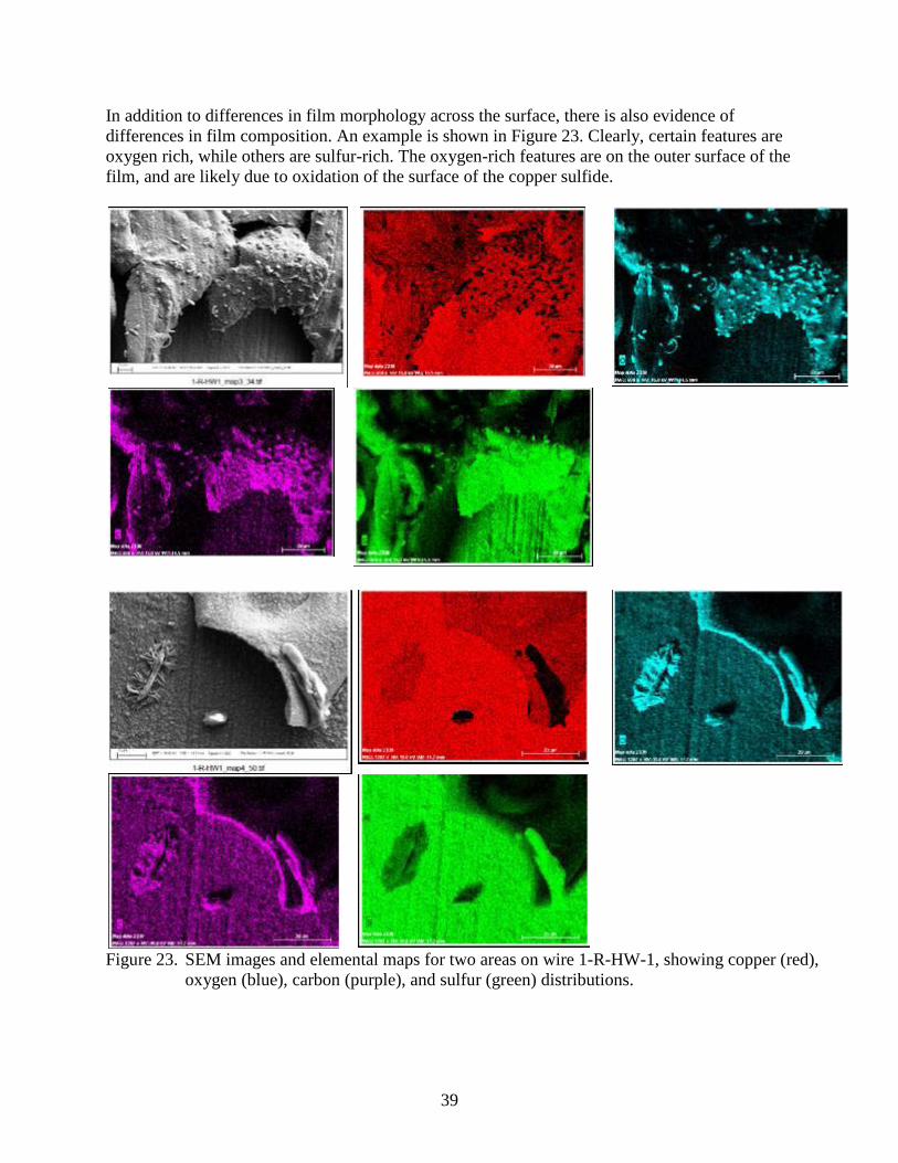
39

In addition to differences in film morphology across the surface, there is also evidence of differences in film composition. An example is shown in Figure 23. Clearly, certain features are oxygen rich, while others are sulfur-rich. The oxygen-rich features are on the outer surface of the film, and are likely due to oxidation of the surface of the copper sulfide.

Figure 23. SEM images and elemental maps for two areas on wire 1-R-HW-1, showing copper (red), oxygen (blue), carbon (purple), and sulfur (green) distributions.

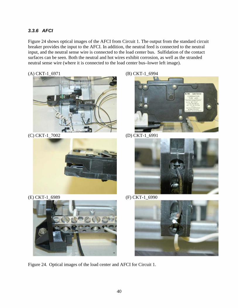
40

3.3.6 AFCI Figure 24 shows optical images of the AFCI from Circuit 1. The output from the standard circuit breaker provides the input to the AFCI. In addition, the neutral feed is connected to the neutral input, and the neutral sense wire is connected to the load center bus. Sulfidation of the contact surfaces can be seen. Both the neutral and hot wires exhibit corrosion, as well as the stranded neutral sense wire (where it is connected to the load center bus–lower left image). (A) CKT-1_6971

(B) CKT-1_6994

(C) CKT-1_7002

(D) CKT-1_6991

(E) CKT-1_6989

(F) CKT-1_6990

Figure 24. Optical images of the load center and AFCI for Circuit 1.

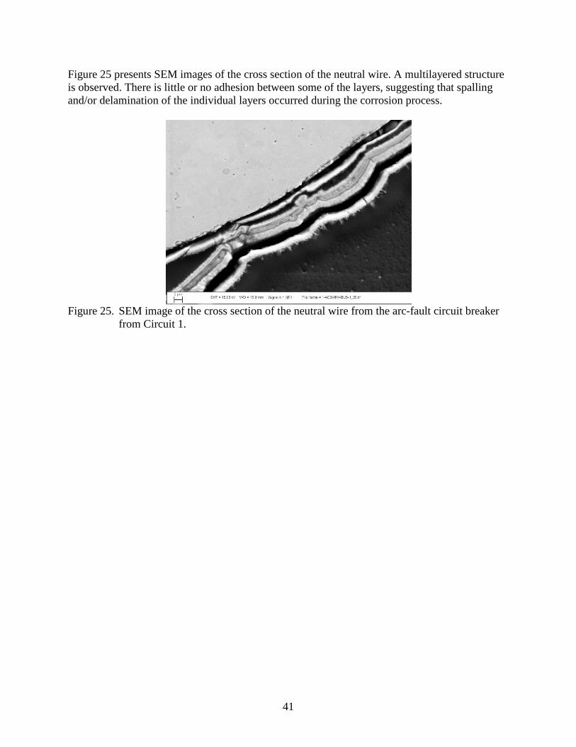
41

Figure 25 presents SEM images of the cross section of the neutral wire. A multilayered structure is observed. There is little or no adhesion between some of the layers, suggesting that spalling and/or delamination of the individual layers occurred during the corrosion process.

Figure 25. SEM image of the cross section of the neutral wire from the arc-fault circuit breaker

from Circuit 1.

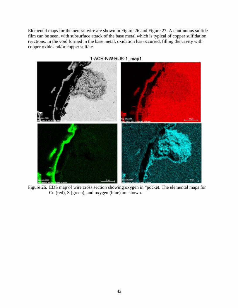
42

Elemental maps for the neutral wire are shown in Figure 26 and Figure 27. A continuous sulfide film can be seen, with subsurface attack of the base metal which is typical of copper sulfidation reactions. In the void formed in the base metal, oxidation has occurred, filling the cavity with copper oxide and/or copper sulfate.

Figure 26. EDS map of wire cross section showing oxygen in “pocket. The elemental maps for

Cu (red), S (green), and oxygen (blue) are shown.

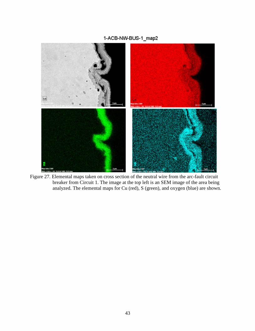
43

Figure 27. Elemental maps taken on cross section of the neutral wire from the arc-fault circuit

breaker from Circuit 1. The image at the top left is an SEM image of the area being analyzed. The elemental maps for Cu (red), S (green), and oxygen (blue) are shown.

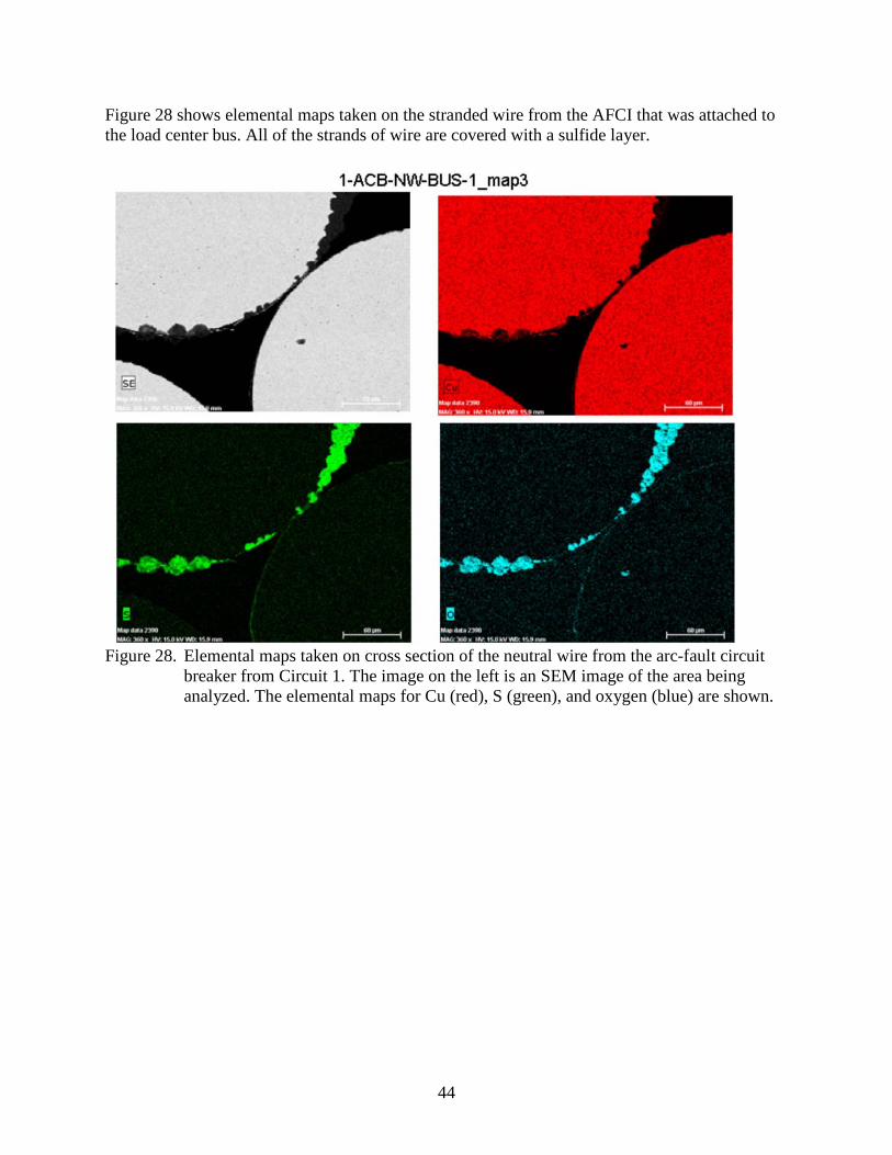
44

Figure 28 shows elemental maps taken on the stranded wire from the AFCI that was attached to the load center bus. All of the strands of wire are covered with a sulfide layer.

Figure 28. Elemental maps taken on cross section of the neutral wire from the arc-fault circuit

breaker from Circuit 1. The image on the left is an SEM image of the area being analyzed. The elemental maps for Cu (red), S (green), and oxygen (blue) are shown.

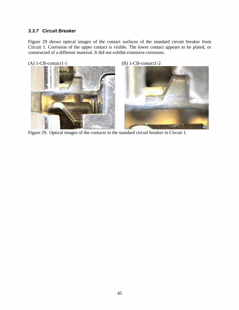
45

3.3.7 Circuit Breaker Figure 29 shows optical images of the contact surfaces of the standard circuit breaker from Circuit 1. Corrosion of the upper contact is visible. The lower contact appears to be plated, or constructed of a different material. It did not exhibit extensive corrosion. (A) 1-CB-contact1-1

(B) 1-CB-contact1-2

Figure 29. Optical images of the contacts in the standard circuit breaker in Circuit 1.

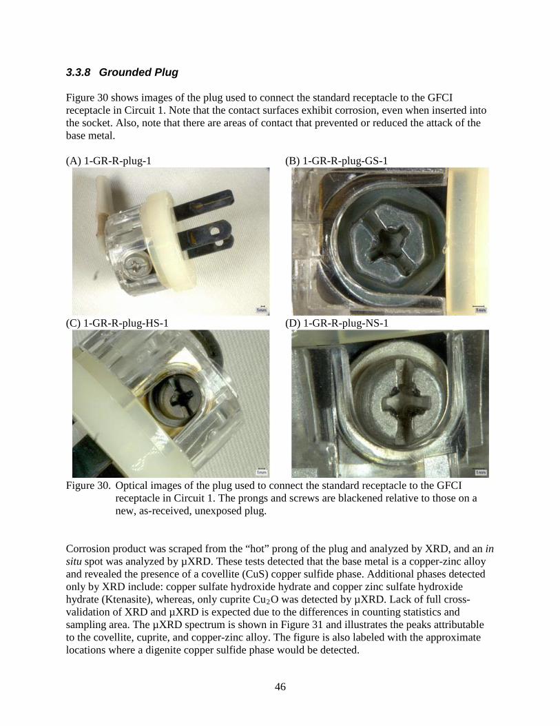
46

3.3.8 Grounded Plug Figure 30 shows images of the plug used to connect the standard receptacle to the GFCI receptacle in Circuit 1. Note that the contact surfaces exhibit corrosion, even when inserted into the socket. Also, note that there are areas of contact that prevented or reduced the attack of the base metal. (A) 1-GR-R-plug-1

(B) 1-GR-R-plug-GS-1

(C) 1-GR-R-plug-HS-1

(D) 1-GR-R-plug-NS-1

Figure 30. Optical images of the plug used to connect the standard receptacle to the GFCI

receptacle in Circuit 1. The prongs and screws are blackened relative to those on a new, as-received, unexposed plug.

Corrosion product was scraped from the “hot” prong of the plug and analyzed by XRD, and an in situ spot was analyzed by µXRD. These tests detected that the base metal is a copper-zinc alloy and revealed the presence of a covellite (CuS) copper sulfide phase. Additional phases detected only by XRD include: copper sulfate hydroxide hydrate and copper zinc sulfate hydroxide hydrate (Ktenasite), whereas, only cuprite Cu2

Figure 31

O was detected by µXRD. Lack of full cross-validation of XRD and µXRD is expected due to the differences in counting statistics and sampling area. The µXRD spectrum is shown in and illustrates the peaks attributable to the covellite, cuprite, and copper-zinc alloy. The figure is also labeled with the approximate locations where a digenite copper sulfide phase would be detected.

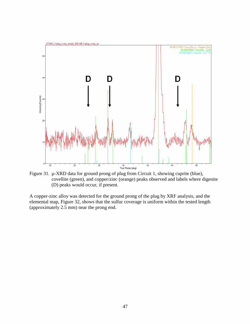
47

Figure 31. µ-XRD data for ground prong of plug from Circuit 1, showing cuprite (blue),

covellite (green), and copper/zinc (orange) peaks observed and labels where digenite (D) peaks would occur, if present.

A copper-zinc alloy was detected for the ground prong of the plug by XRF analysis, and the elemental map, Figure 32, shows that the sulfur coverage is uniform within the tested length (approximately 2.5 mm) near the prong end.

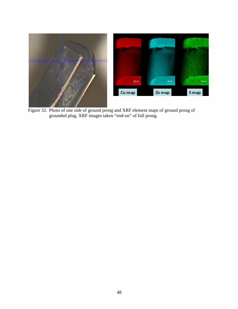
48

Figure 32. Photo of one side of ground prong and XRF element maps of ground prong of grounded plug. XRF images taken “end-on” of full prong.

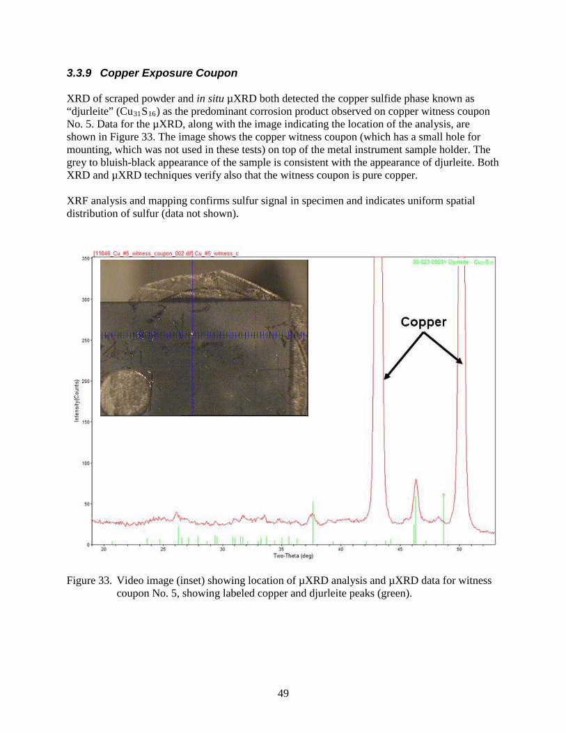
49

3.3.9 Copper Exposure Coupon XRD of scraped powder and in situ µXRD both detected the copper sulfide phase known as “djurleite” (Cu31S16

Figure 33

) as the predominant corrosion product observed on copper witness coupon No. 5. Data for the µXRD, along with the image indicating the location of the analysis, are shown in . The image shows the copper witness coupon (which has a small hole for mounting, which was not used in these tests) on top of the metal instrument sample holder. The grey to bluish-black appearance of the sample is consistent with the appearance of djurleite. Both XRD and µXRD techniques verify also that the witness coupon is pure copper. XRF analysis and mapping confirms sulfur signal in specimen and indicates uniform spatial distribution of sulfur (data not shown).

Figure 33. Video image (inset) showing location of µXRD analysis and µXRD data for witness

coupon No. 5, showing labeled copper and djurleite peaks (green).

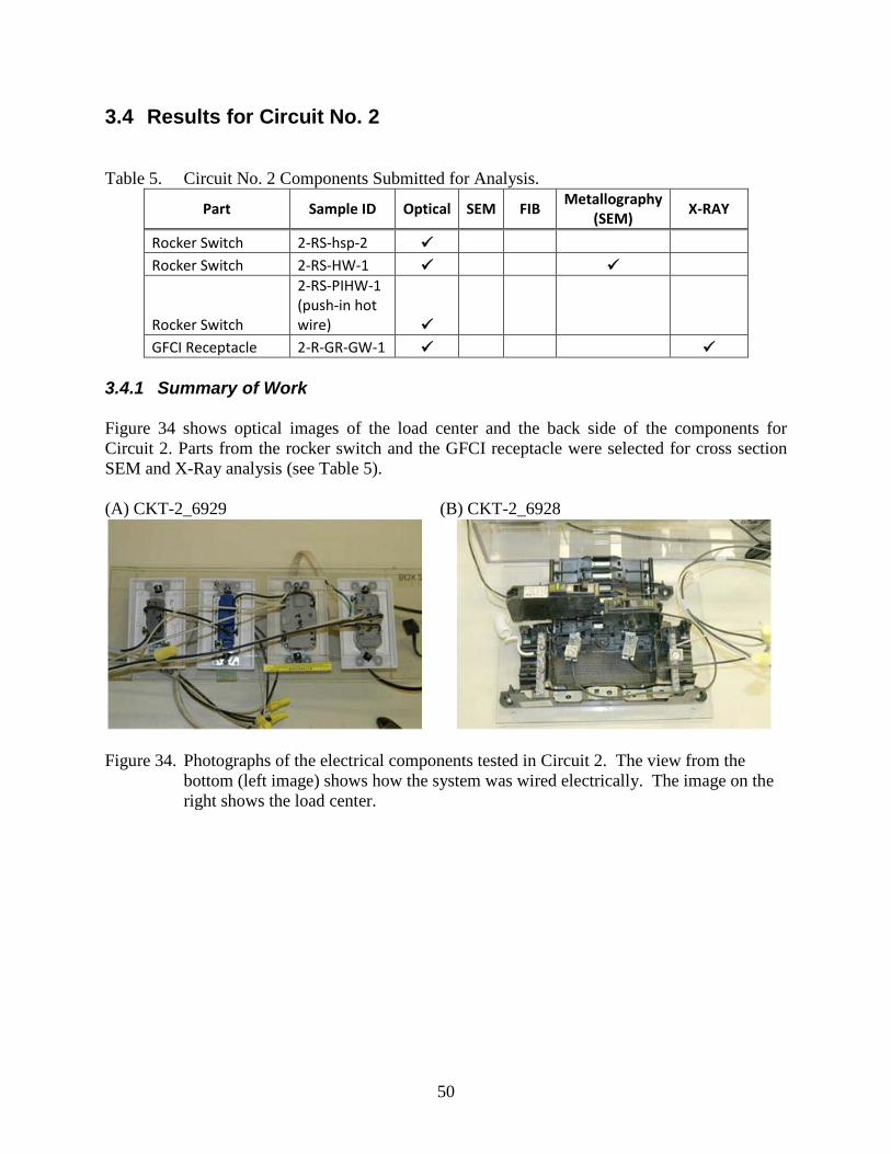
50

3.4 Results for Circuit No. 2 Table 5. Circuit No. 2 Components Submitted for Analysis.

Part Sample ID Optical SEM FIB Metallography

(SEM) X-RAY

Rocker Switch 2-RS-hsp-2 Rocker Switch 2-RS-HW-1

Rocker Switch

2-RS-PIHW-1 (push-in hot wire)

GFCI Receptacle 2-R-GR-GW-1 3.4.1 Summary of Work Figure 34 shows optical images of the load center and the back side of the components for Circuit 2. Parts from the rocker switch and the GFCI receptacle were selected for cross section SEM and X-Ray analysis (see Table 5). (A) CKT-2_6929

(B) CKT-2_6928

Figure 34. Photographs of the electrical components tested in Circuit 2. The view from the bottom (left image) shows how the system was wired electrically. The image on the right shows the load center.

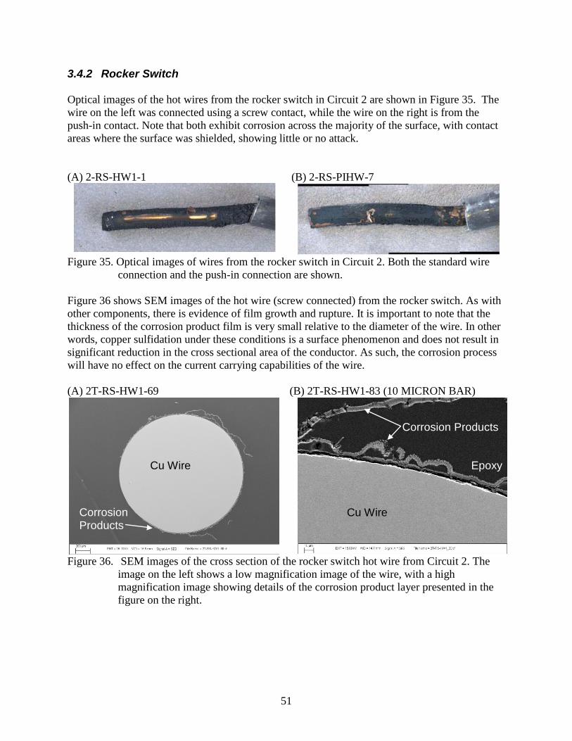
51

3.4.2 Rocker Switch Optical images of the hot wires from the rocker switch in Circuit 2 are shown in Figure 35. The wire on the left was connected using a screw contact, while the wire on the right is from the push-in contact. Note that both exhibit corrosion across the majority of the surface, with contact areas where the surface was shielded, showing little or no attack. (A) 2-RS-HW1-1

(B) 2-RS-PIHW-7

Figure 35. Optical images of wires from the rocker switch in Circuit 2. Both the standard wire

connection and the push-in connection are shown. Figure 36 shows SEM images of the hot wire (screw connected) from the rocker switch. As with other components, there is evidence of film growth and rupture. It is important to note that the thickness of the corrosion product film is very small relative to the diameter of the wire. In other words, copper sulfidation under these conditions is a surface phenomenon and does not result in significant reduction in the cross sectional area of the conductor. As such, the corrosion process will have no effect on the current carrying capabilities of the wire. (A) 2T-RS-HW1-69

(B) 2T-RS-HW1-83 (10 MICRON BAR)

Figure 36. SEM images of the cross section of the rocker switch hot wire from Circuit 2. The

image on the left shows a low magnification image of the wire, with a high magnification image showing details of the corrosion product layer presented in the figure on the right.

Cu Wire

Cu Wire

Epoxy

Corrosion Products

Corrosion Products

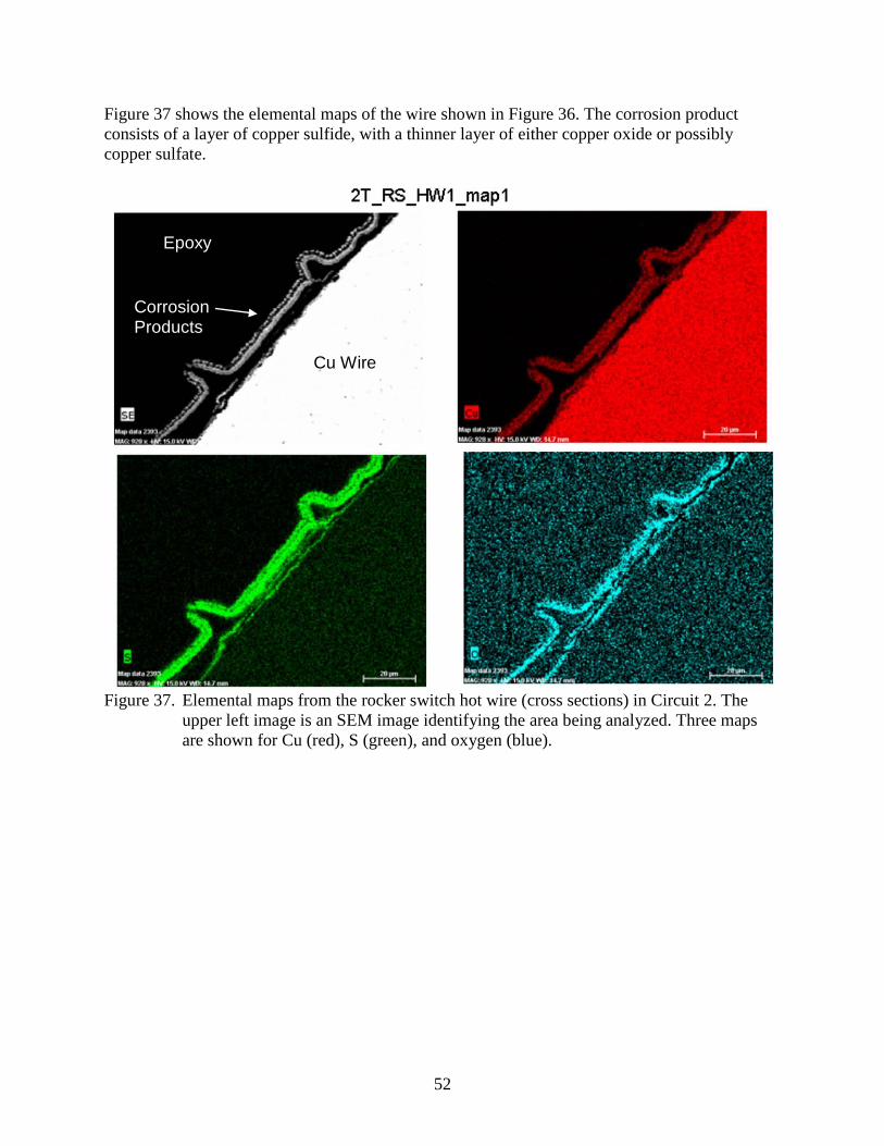
52

Figure 37 shows the elemental maps of the wire shown in Figure 36. The corrosion product consists of a layer of copper sulfide, with a thinner layer of either copper oxide or possibly copper sulfate.

Figure 37. Elemental maps from the rocker switch hot wire (cross sections) in Circuit 2. The

upper left image is an SEM image identifying the area being analyzed. Three maps are shown for Cu (red), S (green), and oxygen (blue).

Cu Wire

Epoxy

Corrosion Products

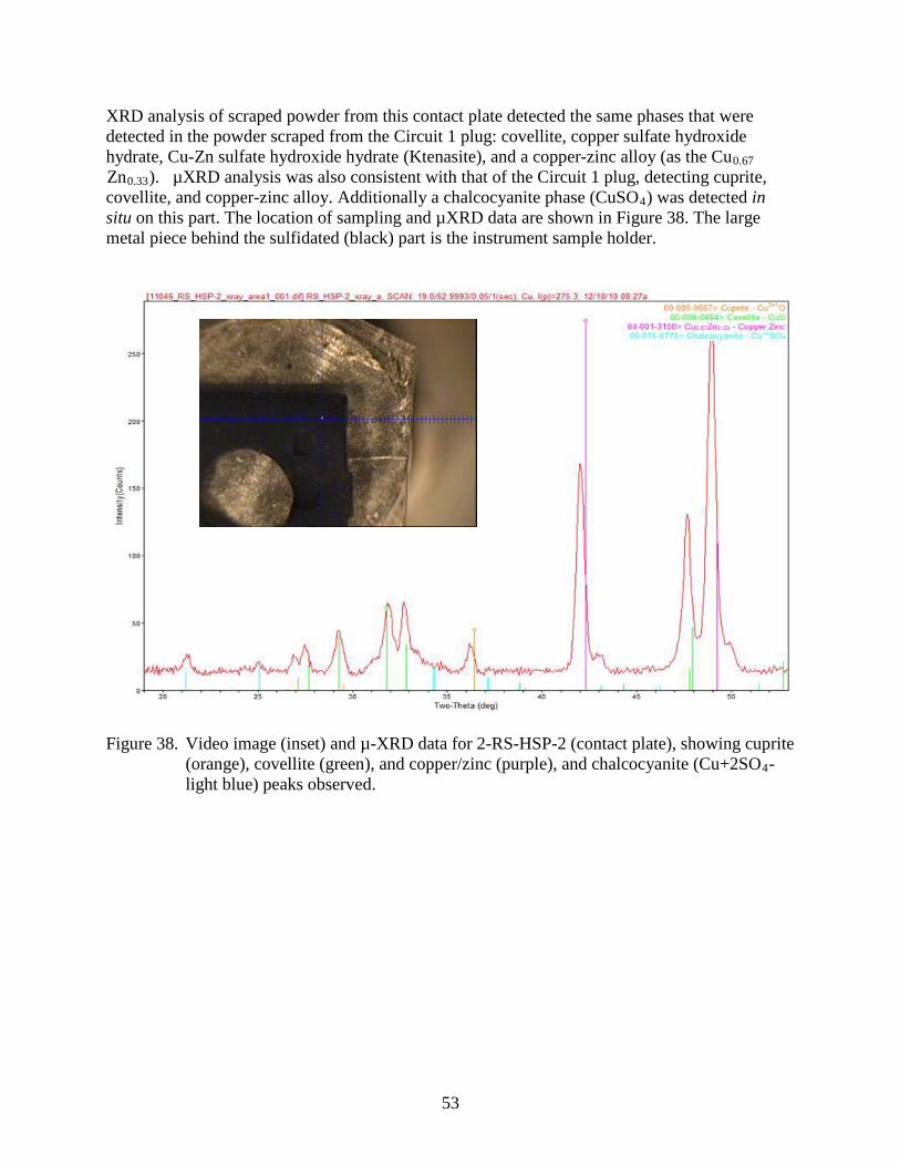
53

XRD analysis of scraped powder from this contact plate detected the same phases that were detected in the powder scraped from the Circuit 1 plug: covellite, copper sulfate hydroxide hydrate, Cu-Zn sulfate hydroxide hydrate (Ktenasite), and a copper-zinc alloy (as the Cu0.67 Zn0.33). µXRD analysis was also consistent with that of the Circuit 1 plug, detecting cuprite, covellite, and copper-zinc alloy. Additionally a chalcocyanite phase (CuSO4

Figure 38) was detected in

situ on this part. The location of sampling and µXRD data are shown in . The large metal piece behind the sulfidated (black) part is the instrument sample holder.

Figure 38. Video image (inset) and µ-XRD data for 2-RS-HSP-2 (contact plate), showing cuprite

(orange), covellite (green), and copper/zinc (purple), and chalcocyanite (Cu+2SO4

- light blue) peaks observed.

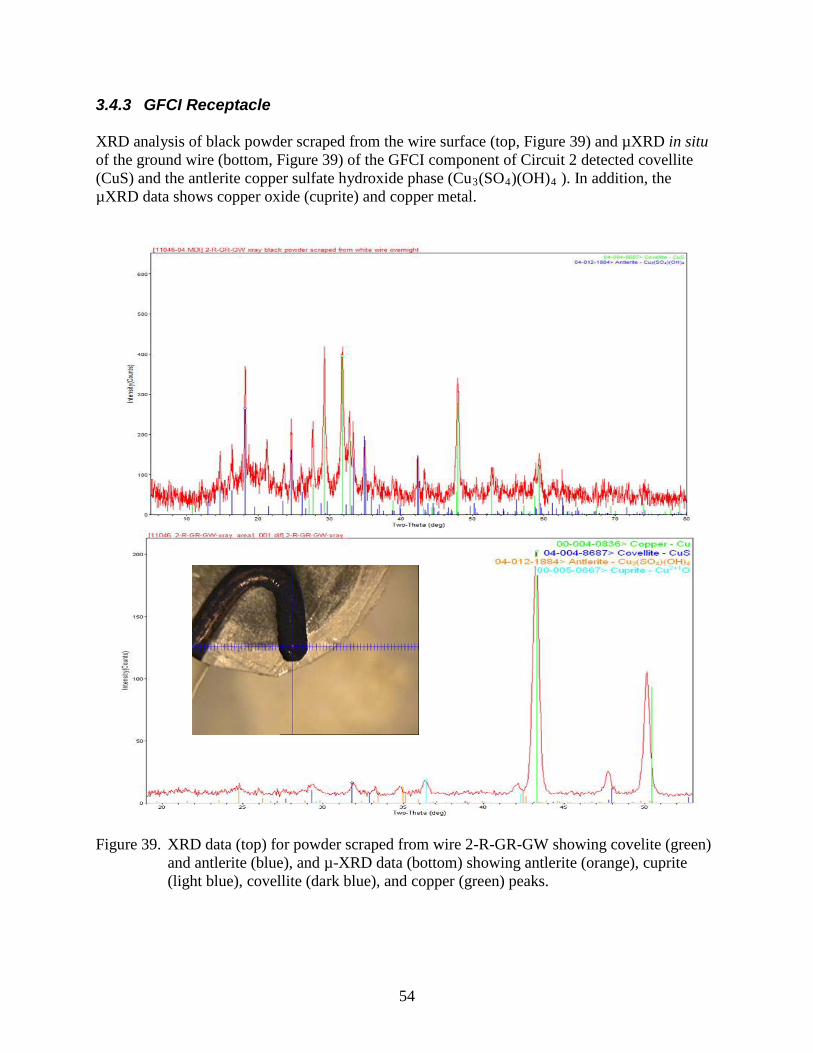
54

3.4.3 GFCI Receptacle XRD analysis of black powder scraped from the wire surface (top, Figure 39) and µXRD in situ of the ground wire (bottom, Figure 39) of the GFCI component of Circuit 2 detected covellite (CuS) and the antlerite copper sulfate hydroxide phase (Cu3(SO4)(OH)4

). In addition, the µXRD data shows copper oxide (cuprite) and copper metal.

Figure 39. XRD data (top) for powder scraped from wire 2-R-GR-GW showing covelite (green)

and antlerite (blue), and µ-XRD data (bottom) showing antlerite (orange), cuprite (light blue), covellite (dark blue), and copper (green) peaks.

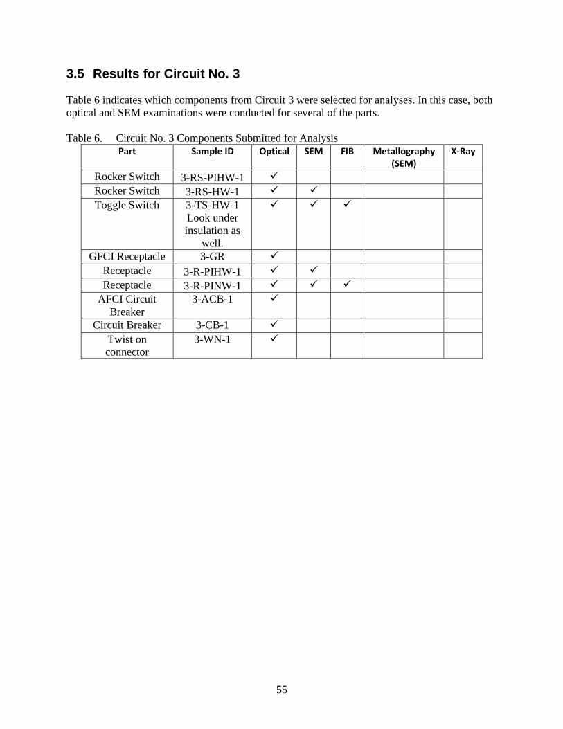
55

3.5 Results for Circuit No. 3 Table 6 indicates which components from Circuit 3 were selected for analyses. In this case, both optical and SEM examinations were conducted for several of the parts. Table 6. Circuit No. 3 Components Submitted for Analysis

Part Sample ID Optical SEM FIB Metallography (SEM)

X-Ray

Rocker Switch 3-RS-PIHW-1 Rocker Switch 3-RS-HW-1 Toggle Switch 3-TS-HW-1

Look under insulation as

well.

GFCI Receptacle 3-GR Receptacle 3-R-PIHW-1 Receptacle 3-R-PINW-1

AFCI Circuit Breaker

3-ACB-1

Circuit Breaker 3-CB-1 Twist on connector

3-WN-1

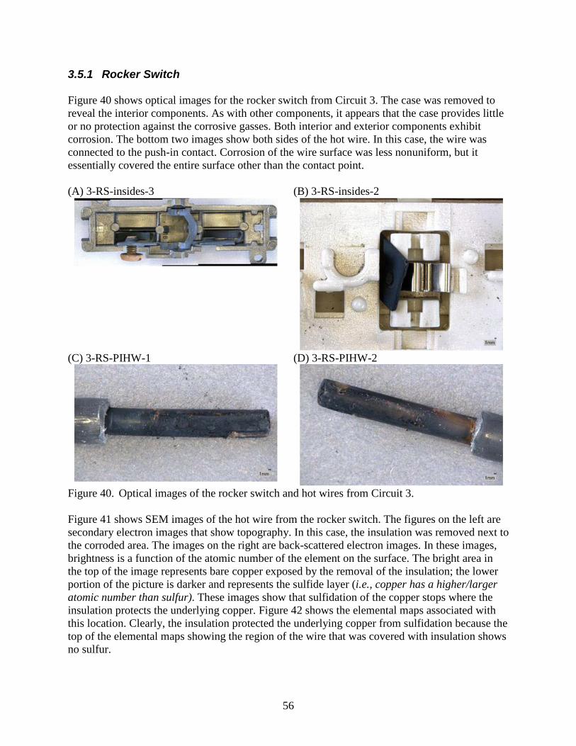
56

3.5.1 Rocker Switch Figure 40 shows optical images for the rocker switch from Circuit 3. The case was removed to reveal the interior components. As with other components, it appears that the case provides little or no protection against the corrosive gasses. Both interior and exterior components exhibit corrosion. The bottom two images show both sides of the hot wire. In this case, the wire was connected to the push-in contact. Corrosion of the wire surface was less nonuniform, but it essentially covered the entire surface other than the contact point. (A) 3-RS-insides-3

(B) 3-RS-insides-2

(C) 3-RS-PIHW-1

(D) 3-RS-PIHW-2

Figure 40. Optical images of the rocker switch and hot wires from Circuit 3. Figure 41 shows SEM images of the hot wire from the rocker switch. The figures on the left are secondary electron images that show topography. In this case, the insulation was removed next to the corroded area. The images on the right are back-scattered electron images. In these images, brightness is a function of the atomic number of the element on the surface. The bright area in the top of the image represents bare copper exposed by the removal of the insulation; the lower portion of the picture is darker and represents the sulfide layer (i.e., copper has a higher/larger atomic number than sulfur). These images show that sulfidation of the copper stops where the insulation protects the underlying copper. Figure 42 shows the elemental maps associated with this location. Clearly, the insulation protected the underlying copper from sulfidation because the top of the elemental maps showing the region of the wire that was covered with insulation shows no sulfur.

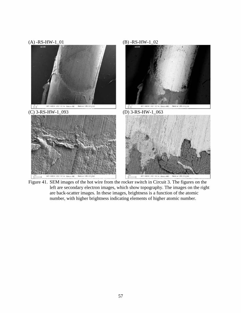
57

(A) -RS-HW-1_01

(B) -RS-HW-1_02

(C) 3-RS-HW-1_093

(D) 3-RS-HW-1_063

Figure 41. SEM images of the hot wire from the rocker switch in Circuit 3. The figures on the

left are secondary electron images, which show topography. The images on the right are back-scatter images. In these images, brightness is a function of the atomic number, with higher brightness indicating elements of higher atomic number.

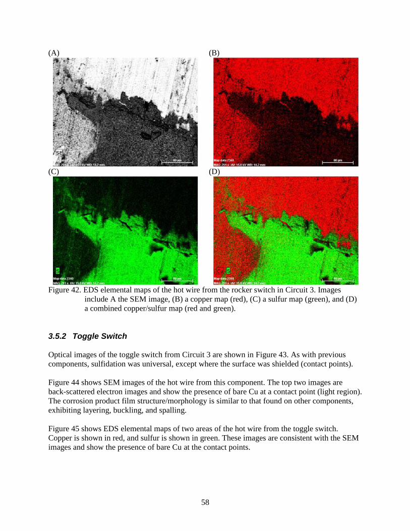
58

(A)

(B)

(C)

(D)

Figure 42. EDS elemental maps of the hot wire from the rocker switch in Circuit 3. Images

include A the SEM image, (B) a copper map (red), (C) a sulfur map (green), and (D) a combined copper/sulfur map (red and green).

3.5.2 Toggle Switch Optical images of the toggle switch from Circuit 3 are shown in Figure 43. As with previous components, sulfidation was universal, except where the surface was shielded (contact points). Figure 44 shows SEM images of the hot wire from this component. The top two images are back-scattered electron images and show the presence of bare Cu at a contact point (light region). The corrosion product film structure/morphology is similar to that found on other components, exhibiting layering, buckling, and spalling. Figure 45 shows EDS elemental maps of two areas of the hot wire from the toggle switch. Copper is shown in red, and sulfur is shown in green. These images are consistent with the SEM images and show the presence of bare Cu at the contact points.

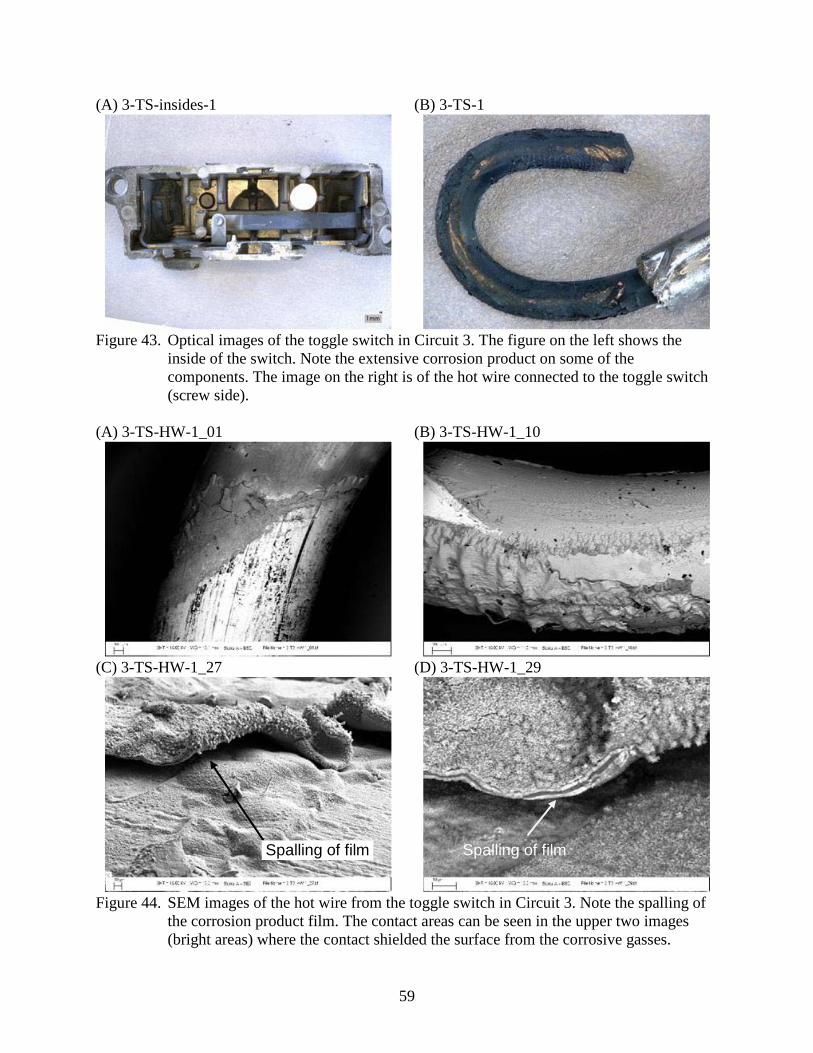
59

(A) 3-TS-insides-1

(B) 3-TS-1

Figure 43. Optical images of the toggle switch in Circuit 3. The figure on the left shows the

inside of the switch. Note the extensive corrosion product on some of the components. The image on the right is of the hot wire connected to the toggle switch (screw side).

(A) 3-TS-HW-1_01

(B) 3-TS-HW-1_10

(C) 3-TS-HW-1_27

(D) 3-TS-HW-1_29

Figure 44. SEM images of the hot wire from the toggle switch in Circuit 3. Note the spalling of

the corrosion product film. The contact areas can be seen in the upper two images (bright areas) where the contact shielded the surface from the corrosive gasses.

Spalling of film Spalling of film

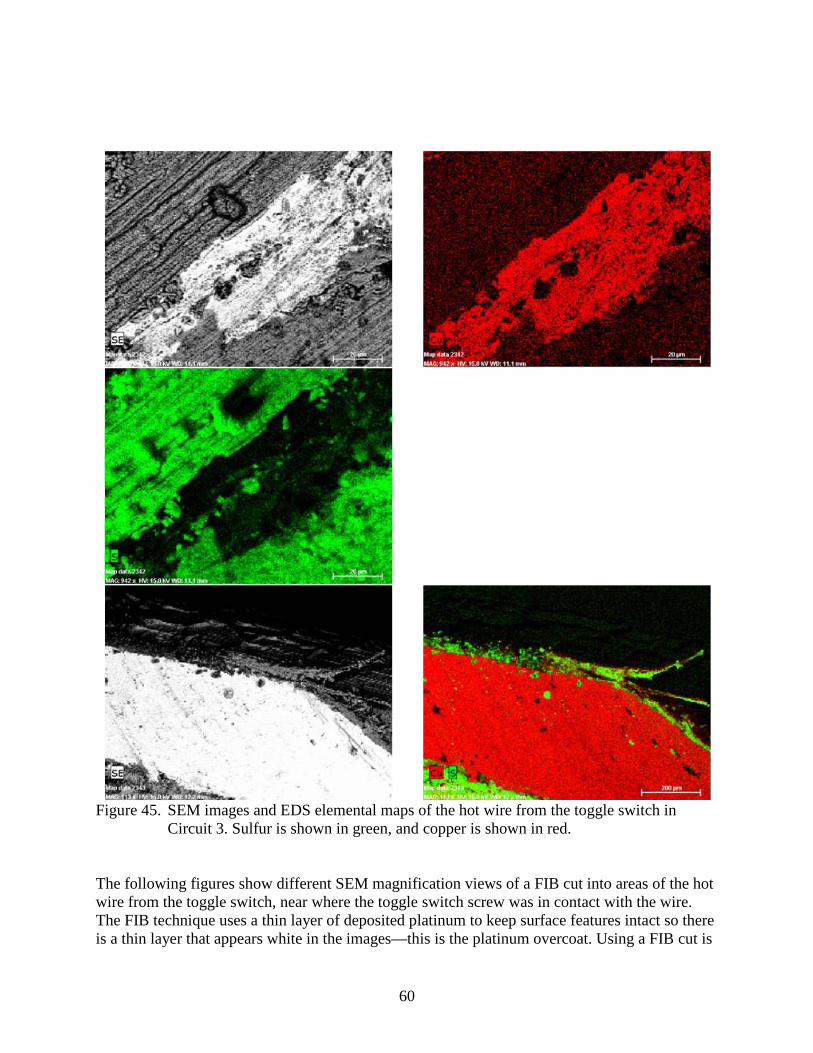
60

Figure 45. SEM images and EDS elemental maps of the hot wire from the toggle switch in

Circuit 3. Sulfur is shown in green, and copper is shown in red. The following figures show different SEM magnification views of a FIB cut into areas of the hot wire from the toggle switch, near where the toggle switch screw was in contact with the wire. The FIB technique uses a thin layer of deposited platinum to keep surface features intact so there is a thin layer that appears white in the images—this is the platinum overcoat. Using a FIB cut is

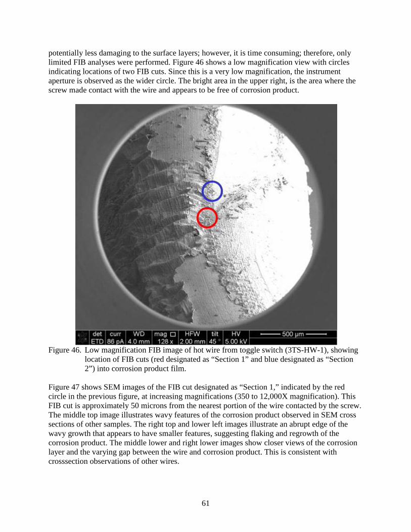
61

potentially less damaging to the surface layers; however, it is time consuming; therefore, only limited FIB analyses were performed. Figure 46 shows a low magnification view with circles indicating locations of two FIB cuts. Since this is a very low magnification, the instrument aperture is observed as the wider circle. The bright area in the upper right, is the area where the screw made contact with the wire and appears to be free of corrosion product.

Figure 46. Low magnification FIB image of hot wire from toggle switch (3TS-HW-1), showing

location of FIB cuts (red designated as “Section 1” and blue designated as “Section 2”) into corrosion product film.

Figure 47 shows SEM images of the FIB cut designated as “Section 1,” indicated by the red circle in the previous figure, at increasing magnifications (350 to 12,000X magnification). This FIB cut is approximately 50 microns from the nearest portion of the wire contacted by the screw. The middle top image illustrates wavy features of the corrosion product observed in SEM cross sections of other samples. The right top and lower left images illustrate an abrupt edge of the wavy growth that appears to have smaller features, suggesting flaking and regrowth of the corrosion product. The middle lower and right lower images show closer views of the corrosion layer and the varying gap between the wire and corrosion product. This is consistent with crosssection observations of other wires.

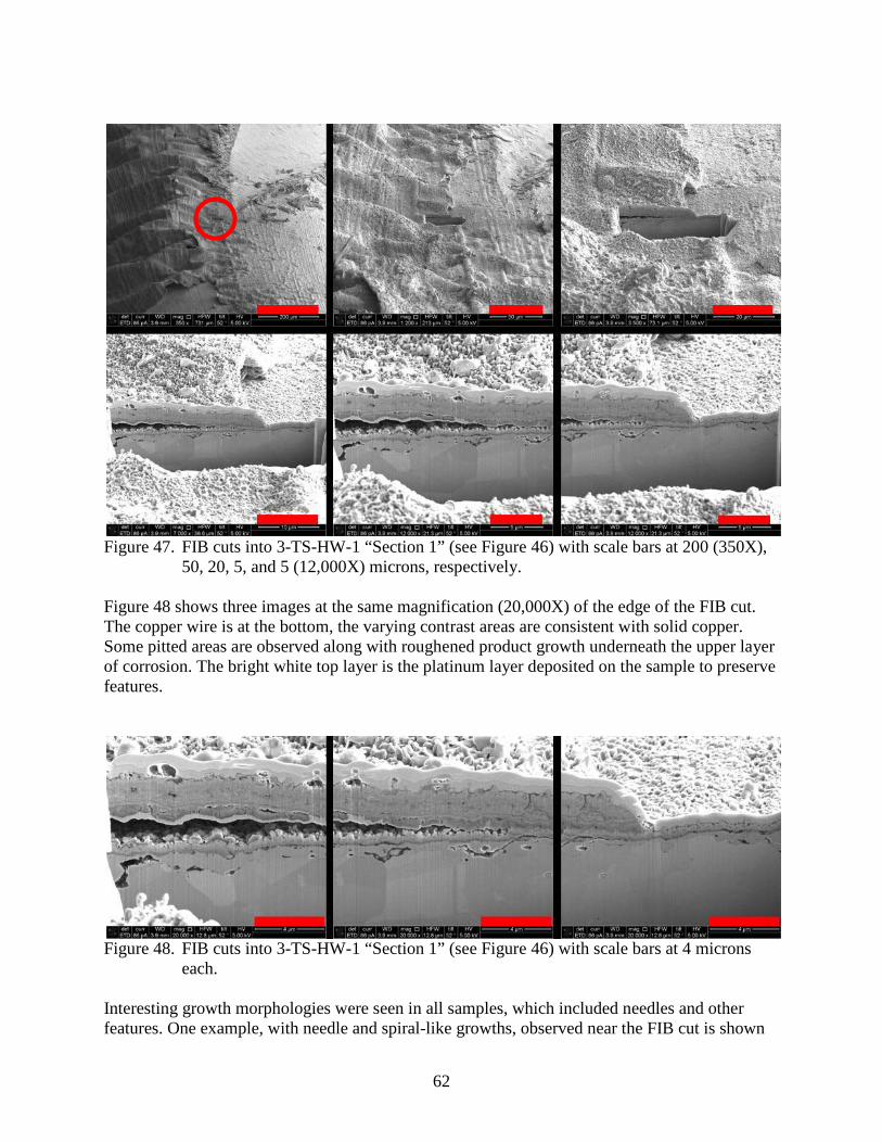
62

Figure 47. FIB cuts into 3-TS-HW-1 “Section 1” (see Figure 46) with scale bars at 200 (350X),

50, 20, 5, and 5 (12,000X) microns, respectively. Figure 48 shows three images at the same magnification (20,000X) of the edge of the FIB cut. The copper wire is at the bottom, the varying contrast areas are consistent with solid copper. Some pitted areas are observed along with roughened product growth underneath the upper layer of corrosion. The bright white top layer is the platinum layer deposited on the sample to preserve features.

Figure 48. FIB cuts into 3-TS-HW-1 “Section 1” (see Figure 46) with scale bars at 4 microns

each. Interesting growth morphologies were seen in all samples, which included needles and other features. One example, with needle and spiral-like growths, observed near the FIB cut is shown

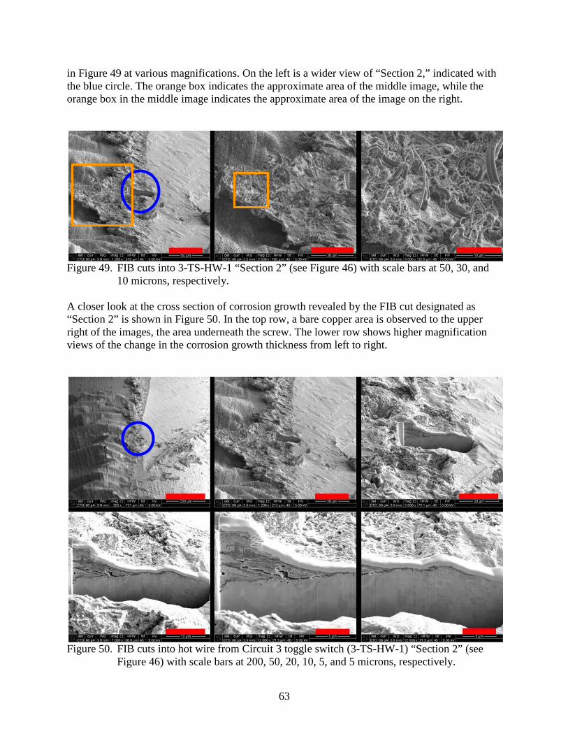
63

in Figure 49 at various magnifications. On the left is a wider view of “Section 2,” indicated with the blue circle. The orange box indicates the approximate area of the middle image, while the orange box in the middle image indicates the approximate area of the image on the right.

Figure 49. FIB cuts into 3-TS-HW-1 “Section 2” (see Figure 46) with scale bars at 50, 30, and

10 microns, respectively. A closer look at the cross section of corrosion growth revealed by the FIB cut designated as “Section 2” is shown in Figure 50. In the top row, a bare copper area is observed to the upper right of the images, the area underneath the screw. The lower row shows higher magnification views of the change in the corrosion growth thickness from left to right.

Figure 50. FIB cuts into hot wire from Circuit 3 toggle switch (3-TS-HW-1) “Section 2” (see

Figure 46) with scale bars at 200, 50, 20, 10, 5, and 5 microns, respectively.

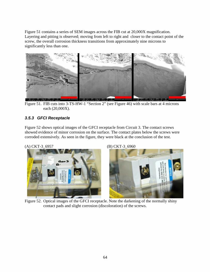
64

Figure 51 contains a series of SEM images across the FIB cut at 20,000X magnification. Layering and pitting is observed; moving from left to right and closer to the contact point of the screw, the overall corrosion thickness transitions from approximately nine microns to significantly less than one.

Figure 51. FIB cuts into 3-TS-HW-1 “Section 2” (see Figure 46) with scale bars at 4 microns

each (20,000X). 3.5.3 GFCI Receptacle Figure 52 shows optical images of the GFCI receptacle from Circuit 3. The contact screws showed evidence of minor corrosion on the surface. The contact plates below the screws were corroded extensively. As seen in the figure, they were black at the conclusion of the test. (A) CKT-3_6957

(B) CKT-3_6960

Figure 52. Optical images of the GFCI receptacle. Note the darkening of the normally shiny

contact pads and slight corrosion (discoloration) of the screws.

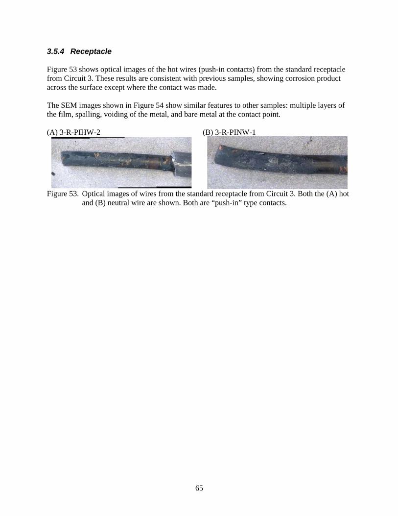
65

3.5.4 Receptacle Figure 53 shows optical images of the hot wires (push-in contacts) from the standard receptacle from Circuit 3. These results are consistent with previous samples, showing corrosion product across the surface except where the contact was made. The SEM images shown in Figure 54 show similar features to other samples: multiple layers of the film, spalling, voiding of the metal, and bare metal at the contact point. (A) 3-R-PIHW-2

(B) 3-R-PINW-1

Figure 53. Optical images of wires from the standard receptacle from Circuit 3. Both the (A) hot

and (B) neutral wire are shown. Both are “push-in” type contacts.

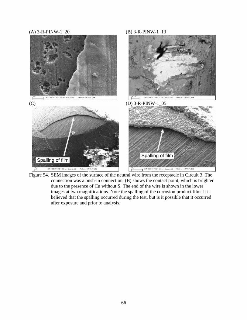
66

(A) 3-R-PINW-1_20

(B) 3-R-PINW-1_13

(C)

(D) 3-R-PINW-1_05

Figure 54. SEM images of the surface of the neutral wire from the receptacle in Circuit 3. The

connection was a push-in connection. (B) shows the contact point, which is brighter due to the presence of Cu without S. The end of the wire is shown in the lower images at two magnifications. Note the spalling of the corrosion product film. It is believed that the spalling occurred during the test, but is it possible that it occurred after exposure and prior to analysis.

Spalling of film Spalling of film

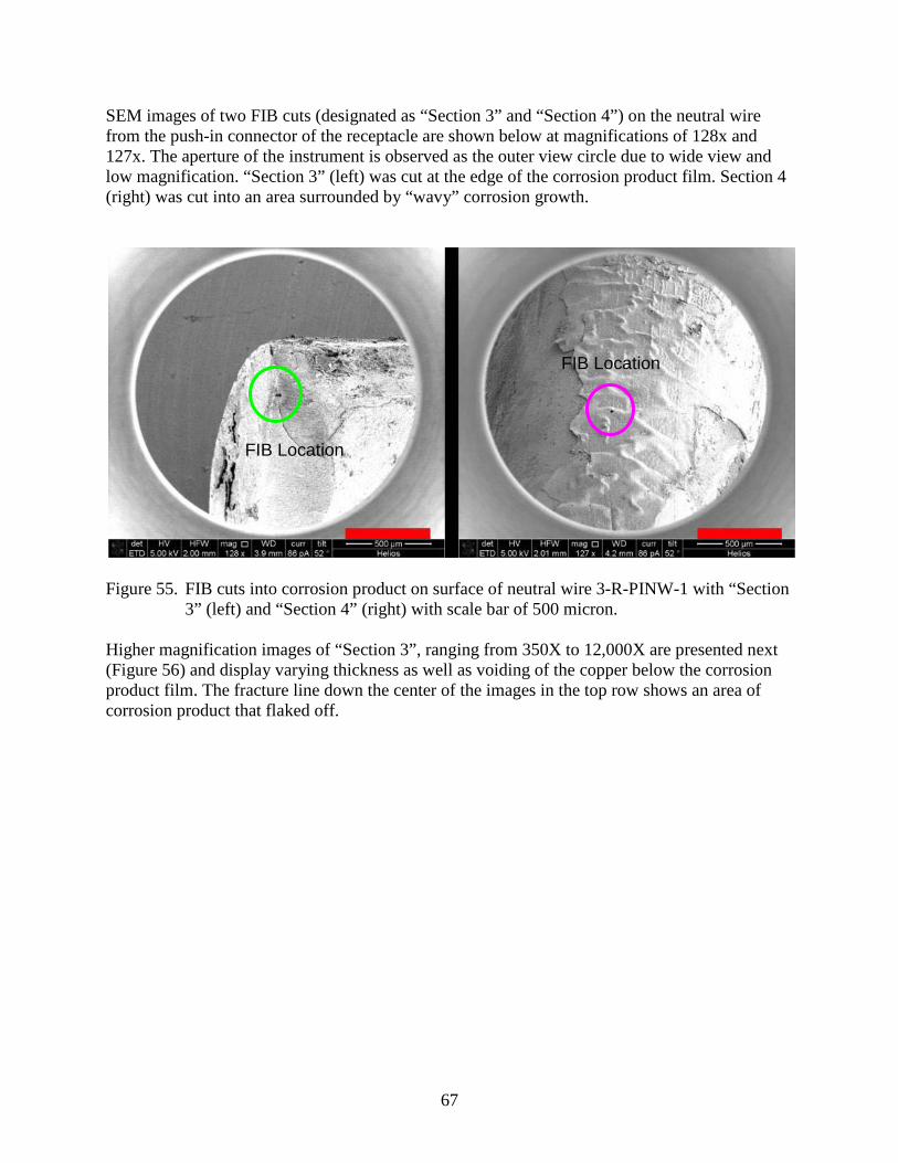
67

SEM images of two FIB cuts (designated as “Section 3” and “Section 4”) on the neutral wire from the push-in connector of the receptacle are shown below at magnifications of 128x and 127x. The aperture of the instrument is observed as the outer view circle due to wide view and low magnification. “Section 3” (left) was cut at the edge of the corrosion product film. Section 4 (right) was cut into an area surrounded by “wavy” corrosion growth.

Figure 55. FIB cuts into corrosion product on surface of neutral wire 3-R-PINW-1 with “Section 3” (left) and “Section 4” (right) with scale bar of 500 micron.

Higher magnification images of “Section 3”, ranging from 350X to 12,000X are presented next (Figure 56) and display varying thickness as well as voiding of the copper below the corrosion product film. The fracture line down the center of the images in the top row shows an area of corrosion product that flaked off.

FIB Location

FIB Location

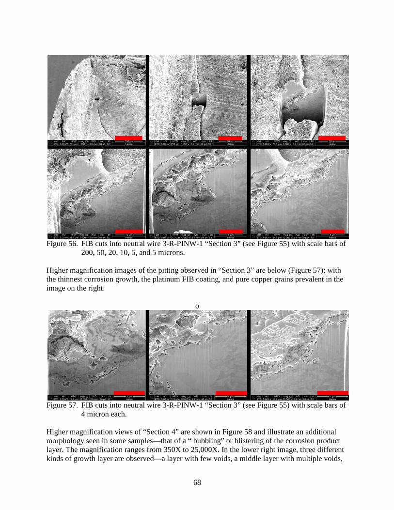
68

Figure 56. FIB cuts into neutral wire 3-R-PINW-1 “Section 3” (see Figure 55) with scale bars of

200, 50, 20, 10, 5, and 5 microns. Higher magnification images of the pitting observed in “Section 3” are below (Figure 57); with the thinnest corrosion growth, the platinum FIB coating, and pure copper grains prevalent in the image on the right.

o

Figure 57. FIB cuts into neutral wire 3-R-PINW-1 “Section 3” (see Figure 55) with scale bars of

4 micron each. Higher magnification views of “Section 4” are shown in Figure 58 and illustrate an additional morphology seen in some samples—that of a “ bubbling” or blistering of the corrosion product layer. The magnification ranges from 350X to 25,000X. In the lower right image, three different kinds of growth layer are observed—a layer with few voids, a middle layer with multiple voids,

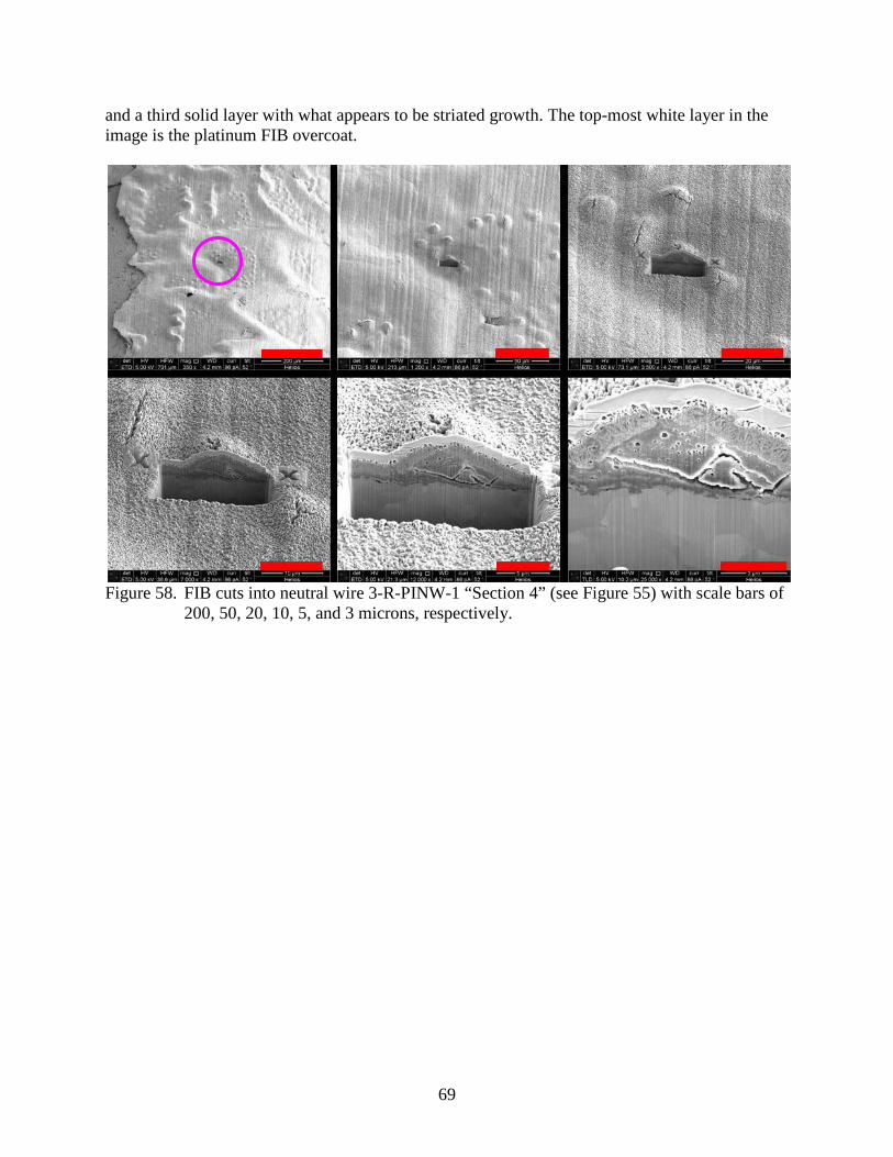
69

and a third solid layer with what appears to be striated growth. The top-most white layer in the image is the platinum FIB overcoat.

Figure 58. FIB cuts into neutral wire 3-R-PINW-1 “Section 4” (see Figure 55) with scale bars of

200, 50, 20, 10, 5, and 3 microns, respectively.

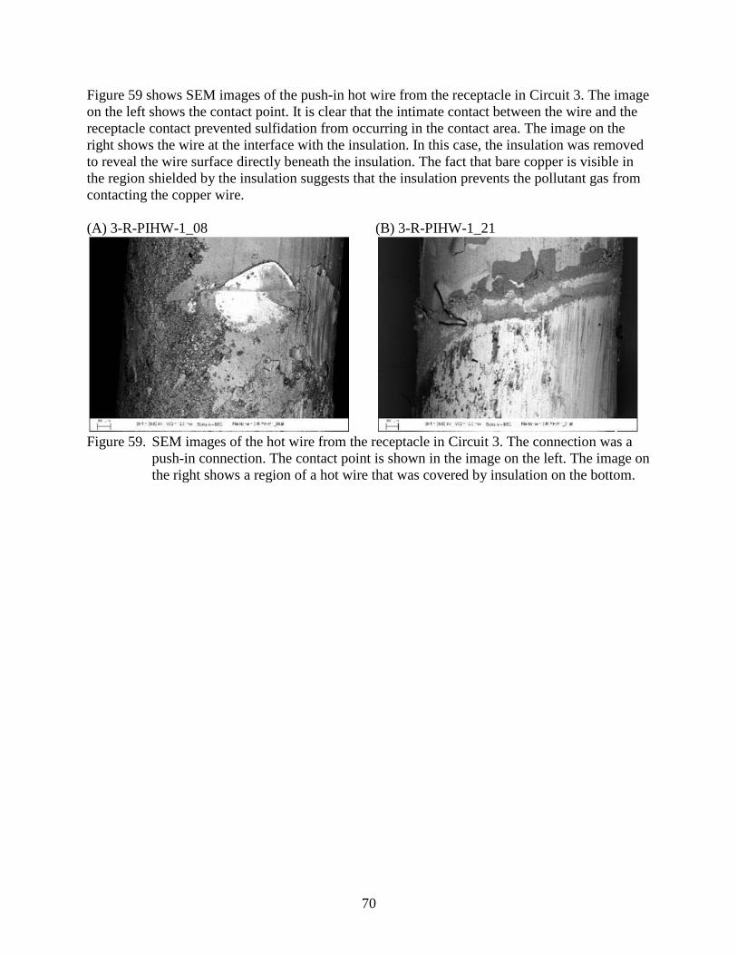
70

Figure 59 shows SEM images of the push-in hot wire from the receptacle in Circuit 3. The image on the left shows the contact point. It is clear that the intimate contact between the wire and the receptacle contact prevented sulfidation from occurring in the contact area. The image on the right shows the wire at the interface with the insulation. In this case, the insulation was removed to reveal the wire surface directly beneath the insulation. The fact that bare copper is visible in the region shielded by the insulation suggests that the insulation prevents the pollutant gas from contacting the copper wire. (A) 3-R-PIHW-1_08

(B) 3-R-PIHW-1_21

Figure 59. SEM images of the hot wire from the receptacle in Circuit 3. The connection was a

push-in connection. The contact point is shown in the image on the left. The image on the right shows a region of a hot wire that was covered by insulation on the bottom.

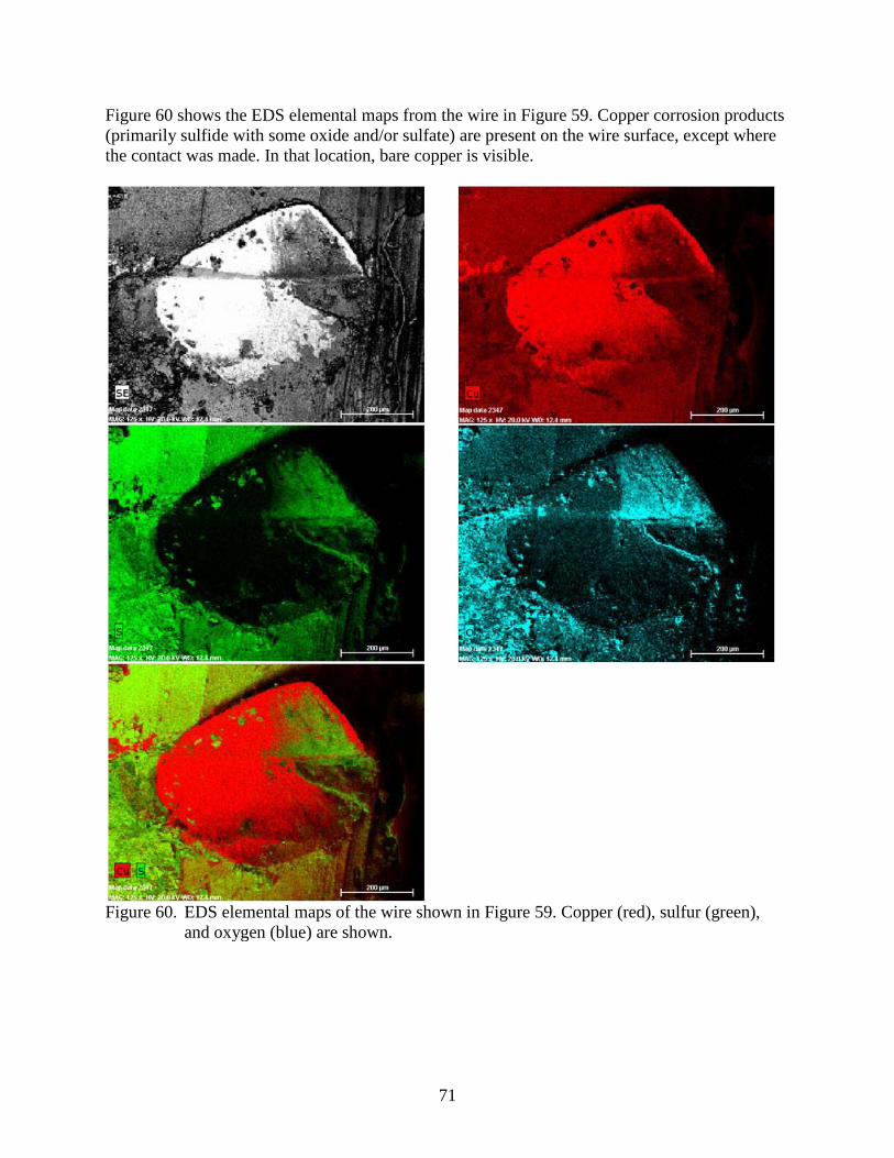
71

Figure 60 shows the EDS elemental maps from the wire in Figure 59. Copper corrosion products (primarily sulfide with some oxide and/or sulfate) are present on the wire surface, except where the contact was made. In that location, bare copper is visible.

Figure 60. EDS elemental maps of the wire shown in Figure 59. Copper (red), sulfur (green), and oxygen (blue) are shown.

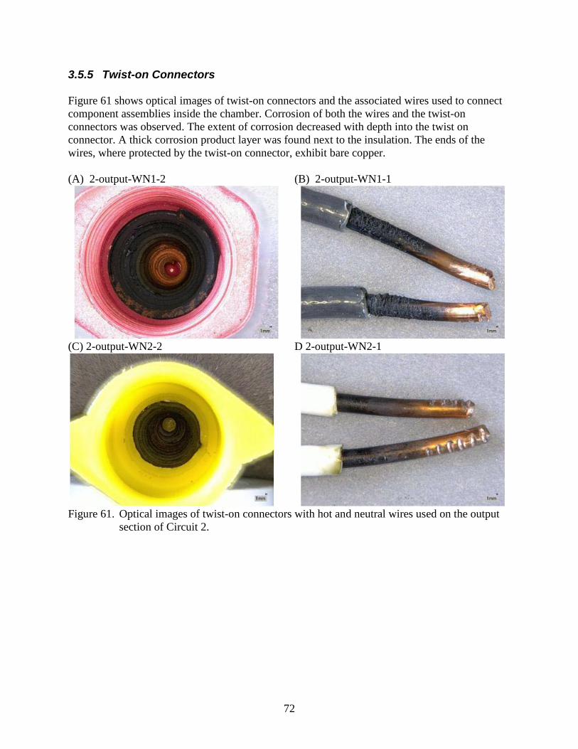
72

3.5.5 Twist-on Connectors Figure 61 shows optical images of twist-on connectors and the associated wires used to connect component assemblies inside the chamber. Corrosion of both the wires and the twist-on connectors was observed. The extent of corrosion decreased with depth into the twist on connector. A thick corrosion product layer was found next to the insulation. The ends of the wires, where protected by the twist-on connector, exhibit bare copper. (A) 2-output-WN1-2

(B) 2-output-WN1-1

(C) 2-output-WN2-2

D 2-output-WN2-1

Figure 61. Optical images of twist-on connectors with hot and neutral wires used on the output

section of Circuit 2.

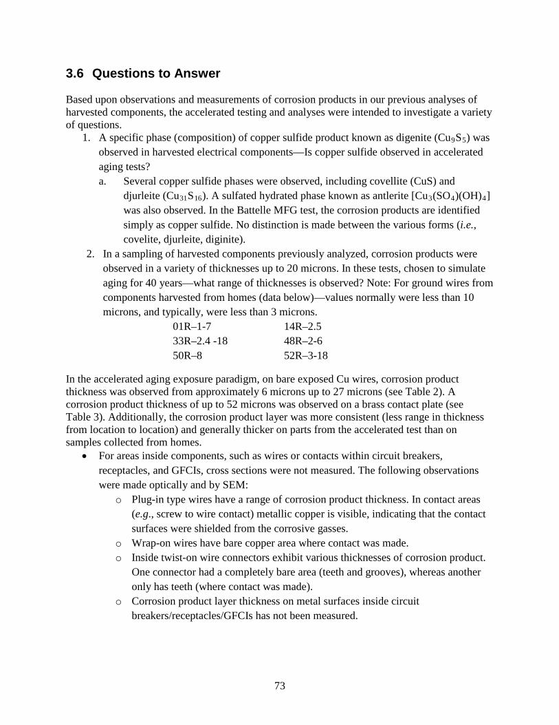
73

3.6 Questions to Answer Based upon observations and measurements of corrosion products in our previous analyses of harvested components, the accelerated testing and analyses were intended to investigate a variety of questions.

1. A specific phase (composition) of copper sulfide product known as digenite (Cu9S5

a. Several copper sulfide phases were observed, including covellite (CuS) and djurleite (Cu

) was observed in harvested electrical components—Is copper sulfide observed in accelerated aging tests?

31S16). A sulfated hydrated phase known as antlerite [Cu3(SO4)(OH)4

2. In a sampling of harvested components previously analyzed, corrosion products were observed in a variety of thicknesses up to 20 microns. In these tests, chosen to simulate aging for 40 years—what range of thicknesses is observed? Note: For ground wires from components harvested from homes (data below)—values normally were less than 10 microns, and typically, were less than 3 microns. 01R–1-7 14R–2.5 33R–2.4 -18 48R–2-6 50R–8 52R–3-18

] was also observed. In the Battelle MFG test, the corrosion products are identified simply as copper sulfide. No distinction is made between the various forms (i.e., covelite, djurleite, diginite).

In the accelerated aging exposure paradigm, on bare exposed Cu wires, corrosion product thickness was observed from approximately 6 microns up to 27 microns (see Table 2). A corrosion product thickness of up to 52 microns was observed on a brass contact plate (see Table 3). Additionally, the corrosion product layer was more consistent (less range in thickness from location to location) and generally thicker on parts from the accelerated test than on samples collected from homes.

• For areas inside components, such as wires or contacts within circuit breakers, receptacles, and GFCIs, cross sections were not measured. The following observations were made optically and by SEM:

o Plug-in type wires have a range of corrosion product thickness. In contact areas (e.g., screw to wire contact) metallic copper is visible, indicating that the contact surfaces were shielded from the corrosive gasses.

o Wrap-on wires have bare copper area where contact was made. o Inside twist-on wire connectors exhibit various thicknesses of corrosion product.

One connector had a completely bare area (teeth and grooves), whereas another only has teeth (where contact was made).

o Corrosion product layer thickness on metal surfaces inside circuit breakers/receptacles/GFCIs has not been measured.

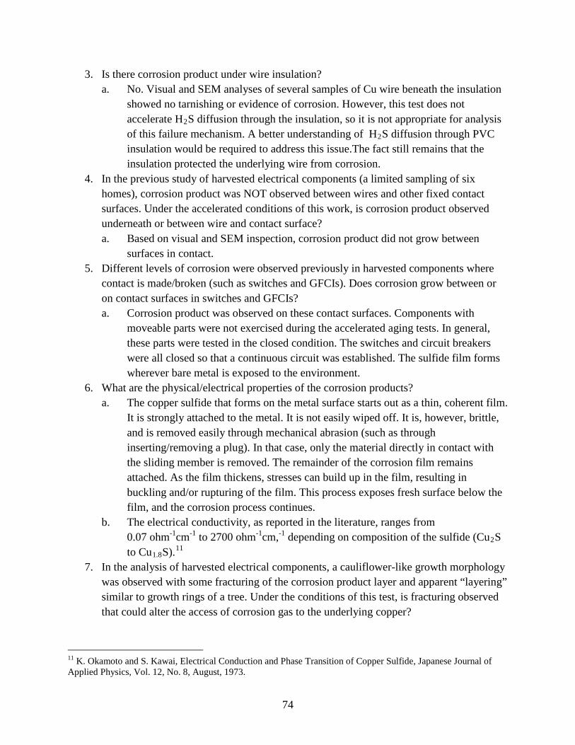
74

3. Is there corrosion product under wire insulation? a. No. Visual and SEM analyses of several samples of Cu wire beneath the insulation

showed no tarnishing or evidence of corrosion. However, this test does not accelerate H2S diffusion through the insulation, so it is not appropriate for analysis of this failure mechanism. A better understanding of H2

4. In the previous study of harvested electrical components (a limited sampling of six homes), corrosion product was NOT observed between wires and other fixed contact surfaces. Under the accelerated conditions of this work, is corrosion product observed underneath or between wire and contact surface?

S diffusion through PVC insulation would be required to address this issue.The fact still remains that the insulation protected the underlying wire from corrosion.

a. Based on visual and SEM inspection, corrosion product did not grow between surfaces in contact.

5. Different levels of corrosion were observed previously in harvested components where contact is made/broken (such as switches and GFCIs). Does corrosion grow between or on contact surfaces in switches and GFCIs? a. Corrosion product was observed on these contact surfaces. Components with

moveable parts were not exercised during the accelerated aging tests. In general, these parts were tested in the closed condition. The switches and circuit breakers were all closed so that a continuous circuit was established. The sulfide film forms wherever bare metal is exposed to the environment.

6. What are the physical/electrical properties of the corrosion products? a. The copper sulfide that forms on the metal surface starts out as a thin, coherent film.

It is strongly attached to the metal. It is not easily wiped off. It is, however, brittle, and is removed easily through mechanical abrasion (such as through inserting/removing a plug). In that case, only the material directly in contact with the sliding member is removed. The remainder of the corrosion film remains attached. As the film thickens, stresses can build up in the film, resulting in buckling and/or rupturing of the film. This process exposes fresh surface below the film, and the corrosion process continues.

b. The electrical conductivity, as reported in the literature, ranges from 0.07 ohm-1cm-1 to 2700 ohm-1cm,-1 depending on composition of the sulfide (Cu2S to Cu1.8S).11

7. In the analysis of harvested electrical components, a cauliflower-like growth morphology was observed with some fracturing of the corrosion product layer and apparent “layering” similar to growth rings of a tree. Under the conditions of this test, is fracturing observed that could alter the access of corrosion gas to the underlying copper?

11 K. Okamoto and S. Kawai, Electrical Conduction and Phase Transition of Copper Sulfide, Japanese Journal of Applied Physics, Vol. 12, No. 8, August, 1973.

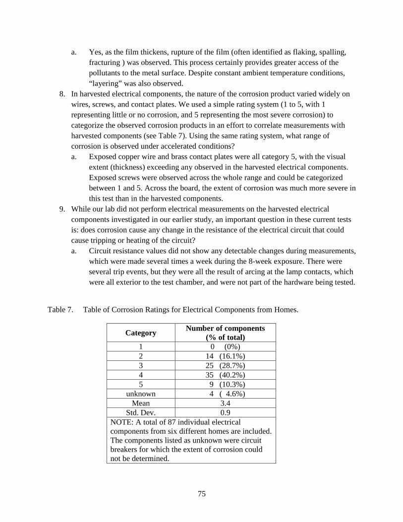
75

a. Yes, as the film thickens, rupture of the film (often identified as flaking, spalling, fracturing ) was observed. This process certainly provides greater access of the pollutants to the metal surface. Despite constant ambient temperature conditions, “layering” was also observed.

8. In harvested electrical components, the nature of the corrosion product varied widely on wires, screws, and contact plates. We used a simple rating system (1 to 5, with 1 representing little or no corrosion, and 5 representing the most severe corrosion) to categorize the observed corrosion products in an effort to correlate measurements with harvested components (see Table 7). Using the same rating system, what range of corrosion is observed under accelerated conditions? a. Exposed copper wire and brass contact plates were all category 5, with the visual

extent (thickness) exceeding any observed in the harvested electrical components. Exposed screws were observed across the whole range and could be categorized between 1 and 5. Across the board, the extent of corrosion was much more severe in this test than in the harvested components.

9. While our lab did not perform electrical measurements on the harvested electrical components investigated in our earlier study, an important question in these current tests is: does corrosion cause any change in the resistance of the electrical circuit that could cause tripping or heating of the circuit? a. Circuit resistance values did not show any detectable changes during measurements,

which were made several times a week during the 8-week exposure. There were several trip events, but they were all the result of arcing at the lamp contacts, which were all exterior to the test chamber, and were not part of the hardware being tested.

Table 7. Table of Corrosion Ratings for Electrical Components from Homes.

Category Number of components (% of total)

1 0 (0%) 2 14 (16.1%) 3 25 (28.7%) 4 35 (40.2%) 5 9 (10.3%)

unknown 4 ( 4.6%) Mean 3.4

Std. Dev. 0.9 NOTE: A total of 87 individual electrical components from six different homes are included. The components listed as unknown were circuit breakers for which the extent of corrosion could not be determined.

76

4. CONCLUSIONS In a previous study, we characterized corrosion products on wires and electrical components harvested from homes by CPSC staff. One result of that study was the conclusion that some components were exposed to environmental conditions that could be classified (in the field of corrosion) as a Battelle Class III or IV. This study, a follow-on to the domestic analysis, was designed to simulate a long duration installation in a household and observe the effects with respect to failure modes, corrosion generated, and any other issues that might affect electrical performance. A variety of commercial, off-the-shelf electrical components (switches, outlets, AFCIs, GFCIs) were enclosed in a chamber for eight weeks under Class IV Battelle environmental conditions and thus, simulated corrosion aging of ~40 years. This type of testing is commonly referred to as “accelerated aging.” Because actual field conditions have not been measured, this is an estimate meant to exceed conditions that might occur over that timeframe in an actual house. Copper sulfide corrosion product characterized in this work exhibited:

• growth on copper-containing components; • growth inside non-hermetically-sealed components (receptacles, breakers, twist-on

connectors); • reduced growth in areas of reduced availability to gas diffusion; • many crystallographic phases; • a wide variety of morphologies; • a range of oxygen content within portions of the product; and • physical features due to flaking, spalling.

Exposed areas of contact screws also exhibited corrosion; however, the copper content or exact composition of corrosion was not measured. The range of corrosion observed, as was observed in the study of harvested components, could be categorized from one to five (representing little or no corrosion to representing the most severe corrosion). The insulation appeared to be very effective in protecting the underlying copper wire. In several instances, the insulation was removed, and no evidence of wire corrosion was seen. These observations cannot be extrapolated to a 40-year lifetime, as the accelerated test would not be expected to accelerate diffusion of sulfur-containing gasses through the PVC insulation. However, the fact remains that the insulated wire, when exposed to a very aggressive environment, did not suffer corrosion beneath the wire insulation. With respect to electrical characteristics and possible hazardous conditions, our testing and materials characterization measurements revealed:

• no growth between surfaces that retained physical contact during testing; • no manifestations of fire or overheating; • no significant detectable changes in circuit resistance (measured via voltage drop); and • no significant degradation of wire cross sectional area.

77

5. IMPLICATIONS The 2009 study was able to identify the nature and extent of the corrosion product that had occurred during the exposure to problem drywall in the six homes, but not how much corrosion could occur for the typical lifetime of household electrical components, and what effects this might have on the electrical function and safety of powered circuits. At the conclusion of this test, copper-containing elements (wires or contact plates) of the electrical components exhibited more extensive (with respect to coverage and thickness) corrosion than any of the components harvested from homes. The corrosion product thickness is small, however, relative to the thickness of any component element. Because the components from this test exhibited no significant loss in cross section, the current carrying capability of the conductors is not expected to be diminished. All of the exposed components functioned throughout the test, with no indication of performance degradation, even though significant corrosion was observed on the copper-based metals. Additionally, no voltage drop (across the entire circuit) was seen, indicating that the presence of the corrosion product film had not resulted in an increase in resistance. There was no intentional activation of the GFCI or AFCI assemblies during the course of the tests. One of the AFCI circuit breakers tripped several times during the test, due to arcing at one of the lamp contacts (external to the exposure chamber), indicating that the functional capabilities had not been compromised. All of these results suggest that the electrical performance and safety of static components or AFCI and GFCI assemblies have not been compromised by the corrosion process. Electrical components, such as rocker switches and contact plates in receptacles that would normally receive both intermittent exposure and intermittent mechanical function in a household installation, were not exercised during the accelerated corrosion test. It is possible that moving metal surfaces relative to one another would remove fragile corrosion layers, reexposing bare metal conductor to the corrosive agent, leading to a higher rate of corrosion and loss of more of the underlying copper as it diffuses to corrosion product layer. Conversely intermittent use and incomplete removal of corrosion could potentially cause a higher resistivity, thus, affecting performance. Further testing that includes functioning of switches and inserting and removing plugs from receptacles is recommended to determine the effect on performance by these specific contact processes. While metal-to-metal contact did not appear to be degraded by the corrosion, exposed metallic parts were corroded, and this likely would render them marginally fit for service (such as in relation to a remediation, they should be replaced).

78

6. DISTRIBUTION

U.S. Consumer Product Safety Commission 4330 East West Highway Bethesda, MD 20814 Attn: Andrew Trotta Mark Gill Sandia National Labs 1 MS0885 Carol Adkins Org. 1800 1 MS0885 Steve Lott Org. 1820 1 MS0886 Jim Aubert Org. 1822 1 MS0886 Curtis Mowry Org. 1822 1 MS0886 Alice C. Kilgo Org. 1822 1 MS0886 Mark A. Rodriquez Org. 1822 1 MS0886 Michael J. Rye Org. 1822 1 MS0886 Bonnie B. McKenzie Org. 1822 1 MS0889 S. Jill Glass Org. 1825 1 MS0889 N. Rob Sorensen Org. 1825 1 MS0889 Samuel J. Lucero Org. 1825 1 MS0899 Technical Library Org. 9536 (electronic copy)