Embed Size (px)
Citation preview

the atmosphere (31, 32). The style of activityimaged requires that the observed slipfaces are notstrongly ice-cemented within the erosion depths.Some of the new grainflow alcoves have widths oftens of meters and have recessed in excess of 10 minto the brink. This implies transport of hundredsof cubicmeters of sand (fig. S1). Even intermediate-sized gullies such as that in Fig. 5 requiremovementof tens of cubic meters of sediment.
The reworking of older gully alcoves by aeolianripples is shown in Fig. 5. The recovery rate of theslipface and the existence of smooth slopes (nograinflows) suggests that grainflow formation andremobilization of sediment by wind may be ap-proximately in equilibrium on a multiyear timescale, although relative rates could vary annually.The seasonal-scale frequency of these two processesdemonstrates active sediment transport on polardunes in the current martian climate. Whether theyindicate migration of martian dune forms or simplyrepresent the crestline maintenance of nonmobiledunes can only be determined with future multiyearobservations.
In locations where wind energy is insufficientto reconstitute grainflow scars, modification ofdune form should ensue. With an estimated sed-iment transport that delivers tens to hundreds ofcubic meters of sand in oneMars year to the dunefoot slopes, the initial modification of dune formwould be rapid. Resulting dune morphologieswould have rounded crests, no brinks, and long,low-angle footslopes. This mechanism may ex-plain some of the unusual dune forms reportedon Mars (33). However, because the majority ofMars’ north polar dunes do not assume this mor-phology, we suggest that maintenance of the
dune form is an active process under the currentmartian climate.
References and Notes1. M. R. Balme, D. Berman, M. Bourke, J. Zimbelman,
Geomorphology 101, 703 (2008).2. J. F. McCauley et al., Icarus 17, 289 (1972).3. J. A. Cutts, R. S. U. Smith, J. Geophys. Res. 78, 4139 (1973).4. H. Tsoar, R. Greeley, A. R. Peterfreund, J. Geophys. Res.
84 (B14), 8167 (1979).5. A. W. Ward, K. B. Doyle, Icarus 55, 420 (1983).6. M. C. Bourke, K. Edgett, B. Cantor, Geomorphology 94,
247 (2008).7. M. C. Bourke et al., Proc. Lunar Planet. Sci. Conf. 40,
1748 (2009).8. V. Schatz, H. Tsoar, K. S. Edgett, E. J. R. Parteli,
H. J. Herrmann, J. Geophys. Res. 111 (E4), E002514 (2006).9. In this paper, we use “frost” and “ice” somewhat
interchangeably. Martian snow has been shown toincrease in density as the winter season progresses (34),so usage of this terminology transitions from one tothe other. Readers are encouraged to understand theuse of either term to be synonymous with “seasonallycondensed volatile.”
10. M. Malin, K. Edgett, J. Geophys. Res. 106 (E10), 23429(2001).
11. C. J. Hansen et al., Bull. Am. Astron. Soc. 40, 409(2008).
12. The numbering of Mars years was defined to facilitatecomparison of data sets across decades and multiple Marsmissions. Year 1 started 11 April 1955.
13. A. McEwen et al., J. Geophys. Res. 112 (E5), E002605(2007).
14. A. Kereszturi et al., Icarus 201, 492 (2009).15. A. Kereszturi et al., Icarus 207, 149 (2010).16. D. Möhlmann, A. Kereszturi, Icarus 207, 654 (2010).17. C. Hansen et al., Proc. Lunar Planet. Sci. Conf. 41,
1533 (2010).18. M. C. Malin, K. Edgett, NASA/JPL Planetary Photojournal,
http://photojournal.jpl.nasa.gov/, catalog no. PIA04290(2005).
19. S. Diniega, S. Byrne, N. T. Bridges, C. M. Dundas,A. S. McEwen, Geology 38, 1047 (2010).
20. E. Gardin, P. Allemand, C. Quantin, P. Thollot,J. Geophys. Res. 115 (E6), E06016 (2010).
21. C. M. Dundas, A. S. McEwen, S. Diniega, S. Byrne,S. Martinez-Alonso, Geophys. Res. Lett. 37, L07202(2009).
22. H. H. Kieffer, Lunar and Planetary Institute contribution1057 (2000).
23. S. Piqueux, P. R. Christensen, J. Geophys. Res. 113 (E6),E06005 (2003).
24. O. Aharonson, 35th Lunar and Planetary ScienceConference, 15 to 19 March 2004, League City, TX, abstr.1918 (2004).
25. H. Kieffer, J. Geophys. Res. 112 (E8), E08005 (2007).26. S. Piqueux, P. R. Christensen, J. Geophys. Res. 113 (E6),
E06005 (2008).27. C. J. Hansen et al., Icarus 205, 283 (2010).28. N. Thomas, C. J. Hansen, G. Portyankina, P. S. Russell,
Icarus 205, 296 (2010).29. G. Portyankina, W. J. Markiewicz, N. Thomas,
C. J. Hansen, M. Milazzo, Icarus 205, 311 (2010).30. S. Silvestro et al., Second International Dunes
Conference, LPI Contributions, 1552, 65 (2010).31. M. Mellon et al., J. Geophys. Res. 114, E00E07
(2009).32. N. Putzig et al., Proc. Lunar Planet. Sci. Conf. 41,
1533 (2010).33. R. Hayward et al., J. Geophys. Res. 112 (E11),
E11007 (2007).34. K. Matsuo, K. Heki, Icarus 202, 90 (2009).35. Ls is the true anomaly of Mars in its orbit around the sun,
measured from the martian vernal equinox, used as a measureof the season on Mars. Ls = 0 corresponds to the beginning ofnorthern spring; Ls = 180 is the beginning of southern spring.
36. This work was partially supported by the Jet PropulsionLaboratory, California Institute of Technology, under acontract with NASA.
Supporting Online Materialwww.sciencemag.org/cgi/content/full/331/6017/575/DC1SOM TextFig. S1References
10 September 2010; accepted 10 January 201110.1126/science.1197636
2500 Years of European ClimateVariability and Human SusceptibilityUlf Büntgen,1,2* Willy Tegel,3 Kurt Nicolussi,4 Michael McCormick,5 David Frank,1,2
Valerie Trouet,1,6 Jed O. Kaplan,7 Franz Herzig,8 Karl-Uwe Heussner,9 Heinz Wanner,2
Jürg Luterbacher,10 Jan Esper11
Climate variations influenced the agricultural productivity, health risk, and conflict level ofpreindustrial societies. Discrimination between environmental and anthropogenic impacts on pastcivilizations, however, remains difficult because of the paucity of high-resolution paleoclimaticevidence. We present tree ring–based reconstructions of central European summer precipitationand temperature variability over the past 2500 years. Recent warming is unprecedented, butmodern hydroclimatic variations may have at times been exceeded in magnitude and duration. Wetand warm summers occurred during periods of Roman and medieval prosperity. Increased climatevariability from ~250 to 600 C.E. coincided with the demise of the western Roman Empire and theturmoil of the Migration Period. Such historical data may provide a basis for counteracting therecent political and fiscal reluctance to mitigate projected climate change.
Continuing global warming and its poten-tial associated threats to ecosystems andhuman health present a substantial chal-
lenge tomodern civilizations that already experiencemany direct and indirect impacts of anthropo-genic climate change (1–4). The rise and fall of
past civilizations have been associated with envi-ronmental change, mainly due to effects on watersupply and agricultural productivity (5–9), hu-man health (10), and civil conflict (11). Althoughmany lines of evidence now point to climate forc-ing as one agent of distinct episodes of societal
crisis, linking environmental variability to humanhistory is still limited by the dearth of high-resolution paleoclimatic data for periods earlier than1000 years ago (12).
Archaeologists have developed oak (Quercusspp.) ring width chronologies from central Europethat cover nearly the entire Holocene and haveused them for the purpose of dating archaeolog-ical artifacts, historical buildings, antique artwork,and furniture (13). The number of samples contrib-uting to these records fluctuates between hundreds
1Swiss Federal Research Institute for Forest, Snow and Land-scape Research (WSL), 8903Birmensdorf, Switzerland. 2OeschgerCentre for Climate Change Research, University of Bern, 3012Bern, Switzerland. 3Institute for ForestGrowth,University of Freiburg,79085 Freiburg, Germany. 4Institute of Geography, University ofInnsbruck, 6020 Innsbruck, Austria. 5Department of History,Harvard University, Cambridge, MA 02138, USA. 6Laboratory ofTree-Ring Research, University of Arizona, Tucson, AZ 85721,USA. 7Environmental Engineering Institute, École PolytechniqueFédérale de Lausanne, 1015 Lausanne, Switzerland. 8BavarianState Department for Cultural Heritage, 86672 Thierhaupten,Germany. 9German Archaeological Institute, 14195 Berlin, Germany.10Department of Geography, Justus LiebigUniversity, 35390Giessen,Germany. 11Department of Geography, Johannes Gutenberg Uni-versity, 55128 Mainz, Germany.
*To whom correspondence should be addressed. E-mail:[email protected]
4 FEBRUARY 2011 VOL 331 SCIENCE www.sciencemag.org578
REPORTS
on
Feb
ruar
y 3,
201
1w
ww
.sci
ence
mag
.org
Dow
nloa
ded
from
and thousands in periods of societal prosperity,whereas fewer samples from periods of socio-economic instability are available (14). Chronol-ogies of living (15) and relict oaks (16, 17) mayreflect distinct patterns of summer precipitationand drought if site ecology and local climatologyimply moisture deficits during the vegetation pe-riod. Annually resolved climate reconstructionsthat contain long-term trends and extend prior tomedieval times, however, depend not only on theinclusion of numerous ancient tree-ring samplesof sufficient climate sensitivity, but also on fre-quency preservation, proxy calibration, and uncer-tainty estimation (18–20).
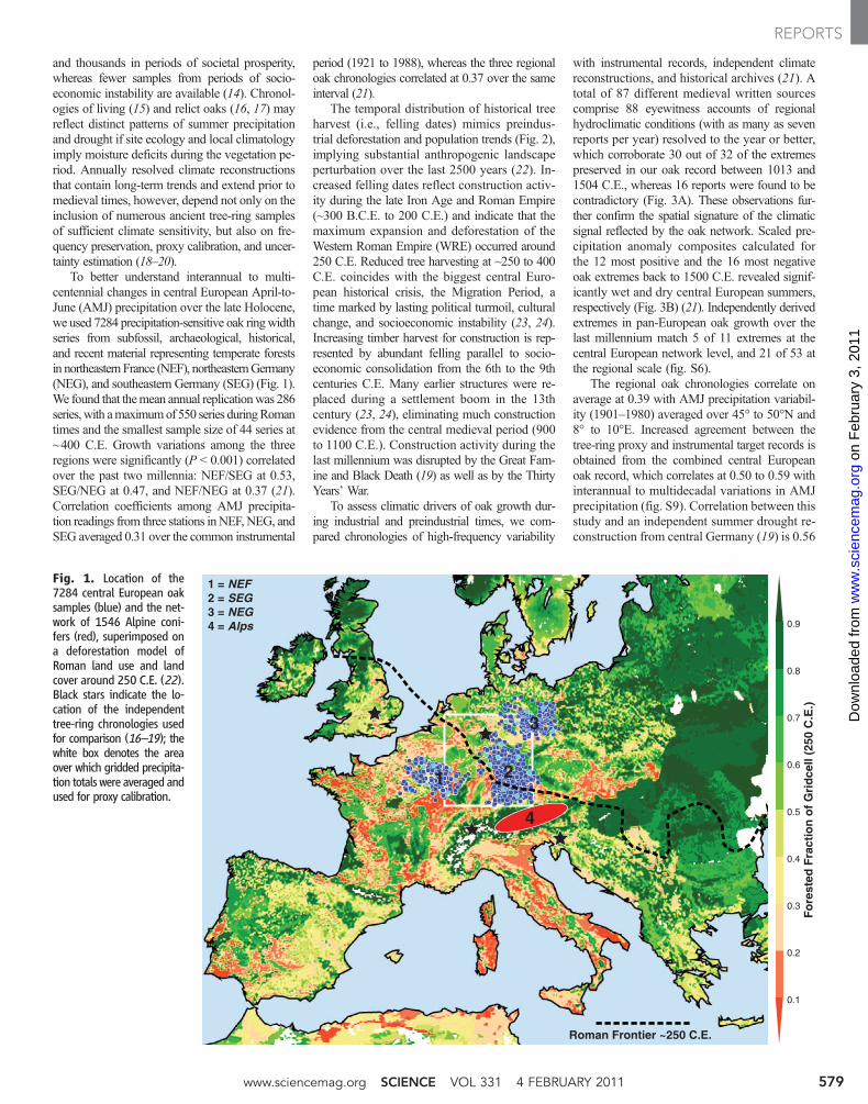
To better understand interannual to multi-centennial changes in central European April-to-June (AMJ) precipitation over the late Holocene,we used 7284 precipitation-sensitive oak ringwidthseries from subfossil, archaeological, historical,and recent material representing temperate forestsin northeastern France (NEF), northeasternGermany(NEG), and southeastern Germany (SEG) (Fig. 1).We found that themean annual replicationwas 286series,with amaximumof 550 series duringRomantimes and the smallest sample size of 44 series at~400 C.E. Growth variations among the threeregions were significantly (P < 0.001) correlatedover the past two millennia: NEF/SEG at 0.53,SEG/NEG at 0.47, and NEF/NEG at 0.37 (21).Correlation coefficients among AMJ precipita-tion readings from three stations inNEF,NEG, andSEG averaged 0.31 over the common instrumental
period (1921 to 1988), whereas the three regionaloak chronologies correlated at 0.37 over the sameinterval (21).
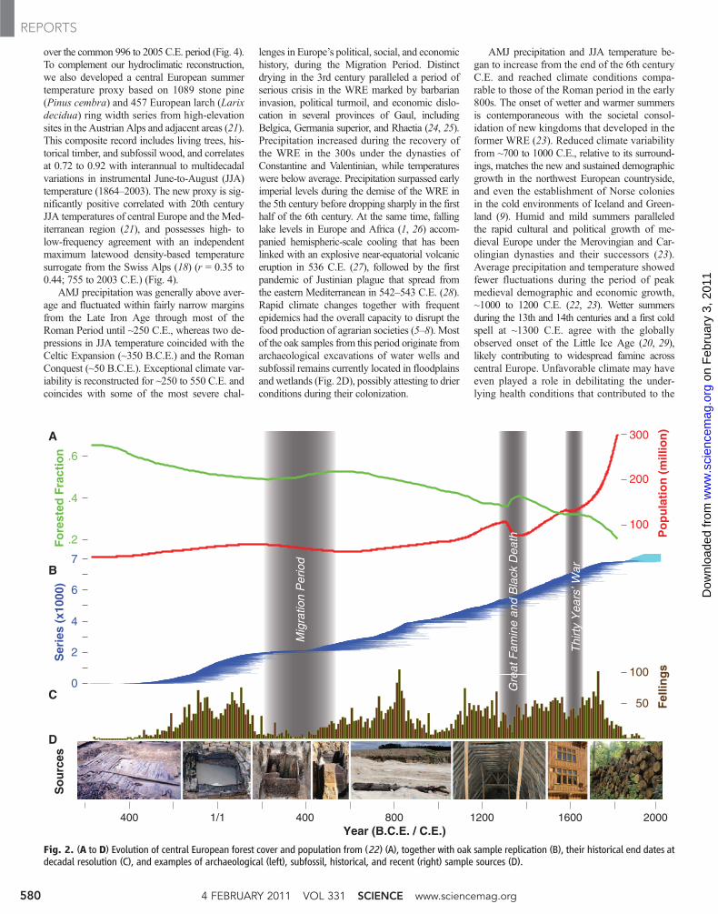
The temporal distribution of historical treeharvest (i.e., felling dates) mimics preindus-trial deforestation and population trends (Fig. 2),implying substantial anthropogenic landscapeperturbation over the last 2500 years (22). In-creased felling dates reflect construction activ-ity during the late Iron Age and Roman Empire(~300 B.C.E. to 200 C.E.) and indicate that themaximum expansion and deforestation of theWestern Roman Empire (WRE) occurred around250 C.E. Reduced tree harvesting at ~250 to 400C.E. coincides with the biggest central Euro-pean historical crisis, the Migration Period, atime marked by lasting political turmoil, culturalchange, and socioeconomic instability (23, 24).Increasing timber harvest for construction is rep-resented by abundant felling parallel to socio-economic consolidation from the 6th to the 9thcenturies C.E. Many earlier structures were re-placed during a settlement boom in the 13thcentury (23, 24), eliminating much constructionevidence from the central medieval period (900to 1100 C.E.). Construction activity during thelast millennium was disrupted by the Great Fam-ine and Black Death (19) as well as by the ThirtyYears’ War.
To assess climatic drivers of oak growth dur-ing industrial and preindustrial times, we com-pared chronologies of high-frequency variability
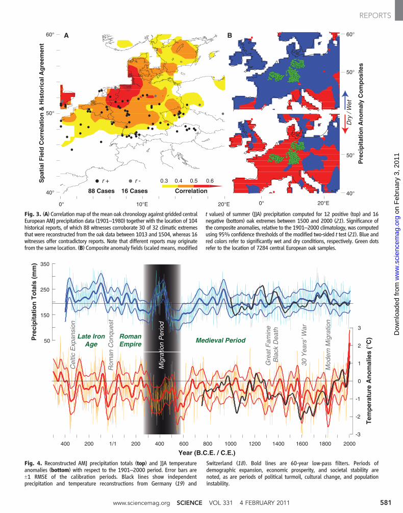
with instrumental records, independent climatereconstructions, and historical archives (21). Atotal of 87 different medieval written sourcescomprise 88 eyewitness accounts of regionalhydroclimatic conditions (with as many as sevenreports per year) resolved to the year or better,which corroborate 30 out of 32 of the extremespreserved in our oak record between 1013 and1504 C.E., whereas 16 reports were found to becontradictory (Fig. 3A). These observations fur-ther confirm the spatial signature of the climaticsignal reflected by the oak network. Scaled pre-cipitation anomaly composites calculated forthe 12 most positive and the 16 most negativeoak extremes back to 1500 C.E. revealed signif-icantly wet and dry central European summers,respectively (Fig. 3B) (21). Independently derivedextremes in pan-European oak growth over thelast millennium match 5 of 11 extremes at thecentral European network level, and 21 of 53 atthe regional scale (fig. S6).
The regional oak chronologies correlate onaverage at 0.39 with AMJ precipitation variabil-ity (1901–1980) averaged over 45° to 50°N and8° to 10°E. Increased agreement between thetree-ring proxy and instrumental target records isobtained from the combined central Europeanoak record, which correlates at 0.50 to 0.59 withinterannual to multidecadal variations in AMJprecipitation (fig. S9). Correlation between thisstudy and an independent summer drought re-construction from central Germany (19) is 0.56
Fig. 1. Location of the7284 central European oaksamples (blue) and the net-work of 1546 Alpine coni-fers (red), superimposed ona deforestation model ofRoman land use and landcover around 250 C.E. (22).Black stars indicate the lo-cation of the independenttree-ring chronologies usedfor comparison (16–19); thewhite box denotes the areaover which gridded precipita-tion totals were averaged andused for proxy calibration.
1
0.2
0.1
1 = NEF2 = SEG3 = NEG4 = Alps
Roman Frontier ~250 C.E.
0.3
0.4
0.5
0.7
0.6
0.8
0.9
Fo
rest
ed F
ract
ion
of
Gri
dce
ll (2
50 C
.E.)
2
3
4
www.sciencemag.org SCIENCE VOL 331 4 FEBRUARY 2011 579
REPORTS
on
Feb
ruar
y 3,
201
1w
ww
.sci
ence
mag
.org
Dow
nloa
ded
from
over the common 996 to 2005 C.E. period (Fig. 4).To complement our hydroclimatic reconstruction,we also developed a central European summertemperature proxy based on 1089 stone pine(Pinus cembra) and 457 European larch (Larixdecidua) ring width series from high-elevationsites in the Austrian Alps and adjacent areas (21).This composite record includes living trees, his-torical timber, and subfossil wood, and correlatesat 0.72 to 0.92 with interannual to multidecadalvariations in instrumental June-to-August (JJA)temperature (1864–2003). The new proxy is sig-nificantly positive correlated with 20th centuryJJA temperatures of central Europe and the Med-iterranean region (21), and possesses high- tolow-frequency agreement with an independentmaximum latewood density-based temperaturesurrogate from the Swiss Alps (18) (r = 0.35 to0.44; 755 to 2003 C.E.) (Fig. 4).
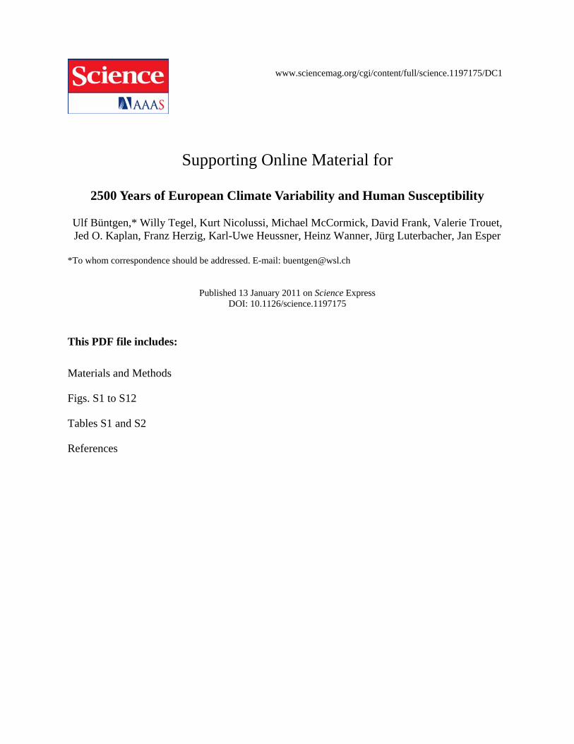
AMJ precipitation was generally above aver-age and fluctuated within fairly narrow marginsfrom the Late Iron Age through most of theRoman Period until ~250 C.E., whereas two de-pressions in JJA temperature coincided with theCeltic Expansion (~350 B.C.E.) and the RomanConquest (~50 B.C.E.). Exceptional climate var-iability is reconstructed for ~250 to 550 C.E. andcoincides with some of the most severe chal-
lenges in Europe’s political, social, and economichistory, during the Migration Period. Distinctdrying in the 3rd century paralleled a period ofserious crisis in the WRE marked by barbarianinvasion, political turmoil, and economic dislo-cation in several provinces of Gaul, includingBelgica, Germania superior, and Rhaetia (24, 25).Precipitation increased during the recovery ofthe WRE in the 300s under the dynasties ofConstantine and Valentinian, while temperatureswere below average. Precipitation surpassed earlyimperial levels during the demise of the WRE inthe 5th century before dropping sharply in the firsthalf of the 6th century. At the same time, fallinglake levels in Europe and Africa (1, 26) accom-panied hemispheric-scale cooling that has beenlinked with an explosive near-equatorial volcaniceruption in 536 C.E. (27), followed by the firstpandemic of Justinian plague that spread fromthe eastern Mediterranean in 542–543 C.E. (28).Rapid climate changes together with frequentepidemics had the overall capacity to disrupt thefood production of agrarian societies (5–8). Mostof the oak samples from this period originate fromarchaeological excavations of water wells andsubfossil remains currently located in floodplainsand wetlands (Fig. 2D), possibly attesting to drierconditions during their colonization.
AMJ precipitation and JJA temperature be-gan to increase from the end of the 6th centuryC.E. and reached climate conditions compa-rable to those of the Roman period in the early800s. The onset of wetter and warmer summersis contemporaneous with the societal consol-idation of new kingdoms that developed in theformer WRE (23). Reduced climate variabilityfrom ~700 to 1000 C.E., relative to its surround-ings, matches the new and sustained demographicgrowth in the northwest European countryside,and even the establishment of Norse coloniesin the cold environments of Iceland and Green-land (9). Humid and mild summers paralleledthe rapid cultural and political growth of me-dieval Europe under the Merovingian and Car-olingian dynasties and their successors (23).Average precipitation and temperature showedfewer fluctuations during the period of peakmedieval demographic and economic growth,~1000 to 1200 C.E. (22, 23). Wetter summersduring the 13th and 14th centuries and a first coldspell at ~1300 C.E. agree with the globallyobserved onset of the Little Ice Age (20, 29),likely contributing to widespread famine acrosscentral Europe. Unfavorable climate may haveeven played a role in debilitating the under-lying health conditions that contributed to the
100
200
300
Po
pu
lati
on
(m
illio
n)
6
7
4
2
0
50
100
.2
.4
.6
Fo
rest
ed F
ract
ion
Ser
ies
(x10
00)
Year (B.C.E. / C.E.)400 1/1 400 800 1200 1600 2000
A
B
C
D
Fel
ling
s
So
urc
es
Mig
ratio
n P
erio
d
Gre
at F
amin
e an
d B
lack
Dea
th
Thi
rty
Yea
rs’ W
ar
D
Fig. 2. (A to D) Evolution of central European forest cover and population from (22) (A), together with oak sample replication (B), their historical end dates atdecadal resolution (C), and examples of archaeological (left), subfossil, historical, and recent (right) sample sources (D).
4 FEBRUARY 2011 VOL 331 SCIENCE www.sciencemag.org580
REPORTS
on
Feb
ruar
y 3,
201
1w
ww
.sci
ence
mag
.org
Dow
nloa
ded
from
50°
40°
0° 10°E
Sp
atia
l Fie
ld C
orr
elat
ion
& H
isto
rica
l Ag
reem
ent
60°
r + r -
20°E
A B
0.6
Correlation16 Cases88 Cases
0.50.40.3
Pre
cip
itat
ion
An
om
aly
Co
mp
osi
tes
0° 20°E
60°
50°
50°
40°
Dry
/ W
et
Fig. 3. (A) Correlationmap of themean oak chronology against gridded centralEuropean AMJ precipitation data (1901–1980) together with the location of 104historical reports, of which 88 witnesses corroborate 30 of 32 climatic extremesthat were reconstructed from the oak data between 1013 and 1504, whereas 16witnesses offer contradictory reports. Note that different reports may originatefrom the same location. (B) Composite anomaly fields (scaledmeans, modified
t values) of summer (JJA) precipitation computed for 12 positive (top) and 16negative (bottom) oak extremes between 1500 and 2000 (21). Significance ofthe composite anomalies, relative to the 1901–2000 climatology, was computedusing 95% confidence thresholds of the modified two-sided t test (21). Blue andred colors refer to significantly wet and dry conditions, respectively. Green dotsrefer to the location of 7284 central European oak samples.
Pre
cip
itat
ion
To
tals
(m
m)
Tem
per
atu
re A
no
mal
ies
(°C
)
Year (B.C.E. / C.E.)400 200 1/1 200 400 600 800 1000 1200 1400 1600 1800 2000
-3
-2
-1
0
1
2
3
Mig
ratio
n P
erio
d
RomanEmpire
Late IronAge
Rom
an C
onqu
est
Cel
tic E
xpan
sion
Medieval Period
Gre
at F
amin
e B
lack
Dea
th
30 Y
ears
’ War
Mod
ern
Mig
ratio
n
50
150
250
350
Fig. 4. Reconstructed AMJ precipitation totals (top) and JJA temperatureanomalies (bottom) with respect to the 1901–2000 period. Error bars areT1 RMSE of the calibration periods. Black lines show independentprecipitation and temperature reconstructions from Germany (19) and
Switzerland (18). Bold lines are 60-year low-pass filters. Periods ofdemographic expansion, economic prosperity, and societal stability arenoted, as are periods of political turmoil, cultural change, and populationinstability.
www.sciencemag.org SCIENCE VOL 331 4 FEBRUARY 2011 581
REPORTS
on
Feb
ruar
y 3,
201
1w
ww
.sci
ence
mag
.org
Dow
nloa
ded
from

devastating economic crisis that arose from thesecond plague pandemic, the BlackDeath, whichreduced the central European population after1347 C.E. by 40 to 60% (19, 22, 28). The periodis also associated with a temperature decline inthe North Atlantic and the abrupt desertion offormer Greenland settlements (9). Temperatureminima in the early 17th and 19th centuries ac-companied sustained settlement abandonmentduring the Thirty Years’ War and the modernmigrations from Europe to America.
The rate of natural precipitation and tem-perature change during the Migration Period mayrepresent a natural analog to rates of projectedanthropogenic climate change. Although mod-ern populations are potentially less vulnerableto climatic fluctuations than past societieshave been, they also are certainly not immuneto the predicted temperature and precipitationchanges, especially considering that migrationto more favorable habitats (22) as an adaptiveresponse will not be an option in an increas-ingly crowded world (6). Comparison of cli-mate variability and human history, however,prohibits any simple causal determination; othercontributing factors such as sociocultural stressorsmust be considered in this complex interplay(7, 30). Nonetheless, the new climate evidencesets a paleoclimatic benchmark in terms of tem-poral resolution, sample replication, and recordlength.
Our data provide independent evidence thatagrarian wealth and overall economic growthmight be related to climate change on high- tomid-frequency (interannual to decadal) time scales.Preindustrial societies were sensitive to famine,disease, and war, which were often driven bydrought, flood, frost or fire events, as indepen-dently described by documentary archives (30).
It also appears to be likely that societies canbetter compensate for abrupt (annual) climaticextremes and have the capacity to adapt toslower (multidecadal to centennial) environmentalchanges (6, 7).
The historical association of precipitationand temperature variation with population mi-gration and settlement desertion in Europe mayprovide a basis for questioning the recent polit-ical and fiscal reluctance to mitigate projectedglobal climate change (31), which reflects the com-mon societal belief that civilizations are insu-lated from variations in the natural environment.
References and Notes1. T. M. Shanahan et al., Science 324, 377 (2009).2. E. R. Cook, R. Seager, M. A. Cane, D. W. Stahle,
Earth Sci. Rev. 81, 93 (2007).3. M. E. Mann, J. D. Woodruff, J. P. Donnelly, Z. Zhang,
Nature 460, 880 (2009).4. E. R. Cook et al., Science 328, 486 (2010).5. B. M. Buckley et al., Proc. Natl. Acad. Sci. U.S.A. 107,
6748 (2010).6. H. Weiss, R. S. Bradley, Science 291, 609
(2001).7. P. B. deMenocal, Science 292, 667 (2001).8. G. H. Haug et al., Science 299, 1731 (2003).9. W. P. Patterson, K. A. Dietrich, C. Holmden, J. T. Andrews,
Proc. Natl. Acad. Sci. U.S.A. 107, 5306 (2010).10. A. J. McMichael, R. E. Woodruff, S. Hales, Lancet 367,
859 (2006).11. M. B. Burke, E. Miguel, S. Satyanath, J. A. Dykema,
D. B. Lobell, Proc. Natl. Acad. Sci. U.S.A. 106, 20670(2009).
12. P. D. Jones et al., Holocene 19, 3 (2009).13. K. Haneca, K. Čufar, H. Beeckman, J. Archaeol. Sci. 36,
1 (2009).14. W. Tegel, J. Vanmoerkerke, U. Büntgen, Quat. Sci. Rev.
29, 1957 (2010).15. D. A. Friedrichs et al., Tree Physiol. 29, 39 (2009).16. P. M. Kelly, H. H. Leuschner, K. R. Briffa, I. C. Harris,
Holocene 12, 689 (2002).17. K. Čufar, M. De Luis, D. Eckstein, L. Kajfez-Bogataj,
Int. J. Biometeorol. 52, 607 (2008).
18. U. Büntgen, D. C. Frank, D. Nievergelt, J. Esper, J. Clim.19, 5606 (2006).
19. U. Büntgen et al., Quat. Sci. Rev. 29, 1005(2010).
20. D. C. Frank et al., Nature 463, 527 (2010).21. See supporting material on Science Online.22. J. O. Kaplan, K. M. Krumhardt, N. Zimmermann,
Quat. Sci. Rev. 28, 3016 (2009).23. M. McCormick, Origins of the European Economy:
Communications and Commerce, A.D. 300–900(Cambridge Univ. Press, Cambridge, 2001).
24. R. Duncan-Jones, in Approaching Late Antiquity: TheTransformation from Early to Late Empire, S. Swain,M. Edwards, Eds. (Oxford Univ. Press, Oxford, 2004),pp. 20–52.
25. C. Witschel, J. Roman Archaeol. 17, 251 (2004).26. D. J. Charman, A. Blundell, R. C. Chiverrell, D. Hendon,
P. G. Langdon, Quat. Sci. Rev. 25, 336 (2006).27. L. B. Larsen et al., Geophys. Res. Lett. 35, L04708
(2008).28. K. L. Kausrud et al., BMC Biol. 8, 112 (2010).29. V. Trouet et al., Science 324, 78 (2009).30. R. Brázdil, C. Pfister, H. Wanner, H. von Storch,
J. Luterbacher, Clim. Change 70, 363 (2005).31. D. B. Lobell et al., Science 319, 607 (2008).32. We thank E. Cook, K. Gibson, G. Haug, G. Huang,
D. Johnson, M. Küttel, N. Stenseth, E. Zorita, and twoanonymous referees for comments and discussion.Supported by the Swiss National Science Foundation(NCCR-Climate), the Deutsche Forschungsgemeinschaftprojects PRIME (62201185) and Paleoclimatology ofthe Middle East (62201236), the Austrian ScienceFund FWF (P15828, F3113-G02), l’Institut Nationalde Recherches Archéologiques Préventives, theAndrew W. Mellon Foundation, and European Unionprojects MILLENNIUM (017008), ACQWA (212250),and CIRCE (036961).
Supporting Online Materialwww.sciencemag.org/cgi/content/full/science.1197175/DC1Materials and MethodsFigs. S1 to S12Tables S1 and S2References
31 August 2010; accepted 5 January 2011Published online 13 January 2011;10.1126/science.1197175
Passive Origins of Stomatal Controlin Vascular PlantsTim J. Brodribb* and Scott A. M. McAdam
Carbon and water flow between plants and the atmosphere is regulated by the opening andclosing of minute stomatal pores in surfaces of leaves. By changing the aperture of stomata,plants regulate water loss and photosynthetic carbon gain in response to many environmentalstimuli, but stomatal movements cannot yet be reliably predicted. We found that thecomplexity that characterizes stomatal control in seed plants is absent in early-divergingvascular plant lineages. Lycophyte and fern stomata are shown to lack key responses toabscisic acid and epidermal cell turgor, making their behavior highly predictable. Theseresults indicate that a fundamental transition from passive to active metabolic control of plantwater balance occurred after the divergence of ferns about 360 million years ago.
The evolution of stomata at least 400 mil-lion years ago (1) enabled plants to trans-form their epidermis into a dynamically
permeable layer that could be either water-tightunder dry conditions or highly permeable to
photosynthetic CO2 during favorable conditions.The combination of adjustable stomata with aninternal water transport system was a turningpoint in plant evolution that enabled vascularplants to invade most terrestrial environments
(2). Today, the leaves of vascular plants possessarrays of densely packed stomata, each onecomprising a pair of adjacent guard cells (Fig.1). High turgor pressure deforms the guard cellsto form an open pore, which allows rapid dif-fusion of atmospheric CO2 through the epidermisinto the photosynthetic tissues inside the leaf.Declining turgor causes the guard cells to closetogether, greatly reducing leaf water loss whilealso restricting entry of CO2 for photosynthesis.Despite the anatomical simplicity of the stomatalvalve, there is little consensus on how angio-sperm stomata sense and respond to theirextrinsic and intrinsic environment. Becausestomata are the gatekeepers of terrestrial photo-synthetic gas exchange, understanding their dy-namic control is imperative for predicting CO2
School of Plant Science, University of Tasmania, Private Bag 55,Hobart, Tasmania 7001, Australia.
*To whom correspondence should be addressed. E-mail:[email protected]
4 FEBRUARY 2011 VOL 331 SCIENCE www.sciencemag.org582
REPORTS
on
Feb
ruar
y 3,
201
1w
ww
.sci
ence
mag
.org
Dow
nloa
ded
from
www.sciencemag.org/cgi/content/full/science.1197175/DC1
Supporting Online Material for
2500 Years of European Climate Variability and Human Susceptibility
Ulf Büntgen,* Willy Tegel, Kurt Nicolussi, Michael McCormick, David Frank, Valerie Trouet, Jed O. Kaplan, Franz Herzig, Karl-Uwe Heussner, Heinz Wanner, Jürg Luterbacher, Jan Esper
*To whom correspondence should be addressed. E-mail: [email protected]
Published 13 January 2011 on Science Express DOI: 10.1126/science.1197175
This PDF file includes: Materials and Methods
Figs. S1 to S12
Tables S1 and S2
References
1
Supporting Online Material for
2500 Years of European Climate Variability and Human
Susceptibility
Ulf Büntgen, Willy Tegel, Kurt Nicolussi, Michael McCormick, David Frank, Valerie Trouet,
Jed Kaplan, Franz Herzig, Karl-Uwe Heussner, Heinz Wanner, Jürg Luterbacher, Jan Esper
The file includes
Materials and methods
Twelve figures and two tables
References
Materials and methods
Oak data. Annually resolved oak ring width measurement series from three regions
(Northeast France = NEF; Northeast Germany = NEG; Southeast Germany = SEG; Table S1)
in Central Europe (CE) were compiled to continuously span the past ~2500 years and cover a
large fraction of temperate forest area north of the Alpine arc and south of the Baltic Sea. The
material contains oak (Quercus robur L. and Q. petraea (Matt.) Liebl.) wood from
archaeological, sub-fossil, and historical surveys, as well as from recent findings. The CE oak
species, Q. robur L. and Q. petraea (Matt.) Liebl., are not anatomically distinguishable (1).
The historical portion of the oak dataset, which clearly represents the majority of the samples
(Table S1), reaches continuously from the Iron Age to the early 20th century. We extended
this dataset into the 21st century following a new approach to overcome the ‘update
desideratum’ of modern site bias: adaptation of the recent to the historical data that was
recently introduced by (2). In this case, recent oak beams and timber were randomly sampled
at different sawmills and lumberyards scattered over the same area from which the historical
2
wood were derived. This random sampling strategy lowers site control and ecological
understanding of the recent material, and typically results in artificial signal-degradation
throughout the modern calibration period. It therefore helps to balance uncertainty-levels over
multi-centennial to millennial-long tree-ring records composed of recent and historical wood
material, and prevents from statistical over-fitting during the proxy/target calibration interval
that ironically coincides with the industrial era (2).
Data adaptation. The three regional oak ring width subsets (NEF, NEG, SEG) and their
CE mean compilation (ALL) were reduced in sample size, i.e., adapted, to test for possible
effects of temporal replication changes on chronology behaviour (Fig. S1, S7; Table S1). The
NEF data were reduced from originally 2880 to an adapted version of only 1025 series. The
NEG data were reduced from 1785 to 833 series, the SEG data from 2619 to 779 series, and
the CE mean dataset (ALL) from 7284 to 2637 series. This data adaptation procedure during
which no new series were created, resulted in a more even distribution of individual series
start and end dates throughout the past ~2500 years (Fig. S1), associated with a more
homogeneous sample replication over time (Fig. S7C). Removal of samples from the original
to the adapted datasets followed a random series selection process applied on highly-
replicated pre-industrial periods from ~200 BC to AD 200, ~AD 400-900 and ~1000-1800, to
roughly match sample size levels of the low-replication intervals from ~AD 200-400, as well
as the 10th and 19th centuries (Fig. S1, Fig. S7C). The resulting adapted datasets and their
subsequent oak chronologies (see below) allowed testing for biases introduced by temporal
changes in sample size. The adaptation method further enabled us to consider possible
uncertainties that might emerge from the integration of predominantly juvenile (fast growing)
or mature/adult (slow growing) wood during specific periods of time.
Growth-trend analysis. Alignment of all individual raw ring width measurement series by
their innermost ring, ideally representing the cambial age, facilitated the assessment of growth
trends and levels (3). The resulting growth curves of the three regions, the so-called Regional
3
Curves (RCs) commonly describe trends of negative exponential shape (3), with very little
differences between the original and adapted subsets (Fig. S2A). An assessment of the mean
segment length (MSL) and average growth rate (AGR) of the raw measurement series
indicated that shorter oak series, containing a greater fraction of juvenile wood, are
characterized by overall higher growth rates, whereas longer series of more mature and adult
wood contain generally lower growth rates (Fig. S2B). This commonly observed association
between MSL and AGR in the raw ring width series emphasizes the need for tree-ring
standardization (detrending) prior to any meaningful interpretation of externally forced
variations (i.e., the putative climatic signal within the oak ring width data must be separated
from the prevailing background noise). The observed similarities in AGR and consistency in
the MSL/AGR association among the various regional subsets denoted their compatibility
also with respect to growth rates and trends.
High-frequency preservation. To maintain inter-annual (high-frequency) variability from
the three regional oak ring width subsets (NEF, NEG and SEG), the original and adapted
subsets of raw measurement series were standardized, i.e., detrended using individual cubic
smoothing splines with 50% frequency-response cut-off at 20 years (4). This detrending
approach has been demonstrated to robustly preserve growth extremes while eliminating
background noise on inter-decadal and longer time-scales (5). Annual ring width indices were
herein calculated as ratios, but also as residuals after the application of a data adaptive power-
transformation applied on the raw measurement series (6). A bi-weight robust mean was used
to generate regional-scale subset chronologies of high-frequency variability. The various oak
chronologies (ratios/original; residuals/original; ratios/adapted; residuals/adapted) per region
were truncated at a minimum replication of five series and normalized over their individual
length. To minimize biases due to replication and inter-series correlation changes, the
normalized time-series were additionally corrected for artificial variance changes by
calculating ratios from 31-year moving standard deviations (7), i.e., the normalized annual
4
chronology indices were divided by the corresponding values of their 31-year moving
standard deviations (Fig. S3). The variance stabilized, regional-scale (high-frequency)
chronologies are most suitable to detect inter-annual growth extremes likely caused by
hydroclimatic anomalies. Nevertheless, they do not contain any information about longer-
term changes in the prevailing climate system or their surrounding environment (5).
Extreme-year validation. We calculated moving 31-year correlation coefficients to assess
the shared inter-annual (high-frequency) variability amongst the three regional subset
chronologies (Fig. S4A). Correlation coefficients amongst the three time-series average at
0.44 over the common 210 BC to AD 1992 period. Higher agreement of r =0.52 was found
over the better-replicated last millennium. Reduced coherency amongst the three regional
chronologies occurred from ~1800 onwards, the period during which the randomly updated
recent data prevail. This recent coherency decline indicates that the proxy/target calibration
results (see below) are likely conservative (2). The variance stabilized high-frequency
chronologies (Fig. S4B) were further used to reconstruct the frequency and severity of annual
growth extremes, which either occurred at the regional-scale, i.e., in two of the three regional
chronologies, or at the sub-continental CE-scale, i.e., common to all three regional oak
chronologies (Fig. S4C). Regional extremes in radial oak growth were defined as occurring
when all four chronologies per region (ratios/original; residuals/original; ratios/adapted;
residuals/adapted) exceeded their corresponding 1.5 standard deviation threshold (5). Sub-
continental CE network extremes occurred when all three regional records shared an extreme
year.
Scaled precipitation anomaly (1961-1990 mean subtracted) composites (8) for CE
summers (June-August) were computed for the oak extremes back to AD 1500 (Fig. S5). In
contrast to the classical compositing technique that uses the arithmetic mean and a t-test for
the means, we applied a scaled mean and modified t-value (8). This method provides more
robust results if the distribution is not ‘Gaussian’, in case of small samples or if there are

5
outliers. Scaled anomaly composites were calculated for the 12 most positive and the 16 most
negative oak extremes back to AD 1500 using gridded precipitation reconstructions (9).
We extracted historical documentary evidence assembled and uploaded to the geo-
database ‘Digital Atlas of Roman and Medieval Civilizations’ (DARMC;
http://darmc.harvard.edu), to verify the climatic signal in the oak extremes further back in
time, i.e., during the first half of the last millennium during which no gridded precipitation
reconstructions exist (9). The early historical records in Latin, Middle Dutch, Middle French,
and Middle German supplied a total of 87 different medieval records, usually eyewitnesses
from or near the regions represented by the oak network. The 87 different records offered 104
reports (since some records report on multiple years) on regional hydroclimatic conditions in
32 extreme years, resolved to the year or better, with 1-7 witnesses per year. A total of 88 out
of 104 reports corroborate 30 out of 32 of the precipitation extremes preserved in our oak
record between 1013 and 1504. Of the 16 contradictory reports, 13 occur for 9 years (AD
1221, 1270, 1309, 1350, 1353, 1368, 1434, 1464, 1487) whose precipitation extremes are in
fact corroborated by 20 (of the 88) confirming historical witnesses. The contradictory reports
for those 9 years may reflect local precipitation variation or simply ambiguity in those
medieval written records. The only three reports that contradict the dendro-data in the absence
of other, corroborating testimony, refer to two poorly documented years (AD 1044, 2 reports,
and 1121, 1 report). Thus the medieval human witnesses independently confirm the skill of
our method for reconstructing precipitation from the proxy data in a time and region where
the anthropogenic impact on climate systems and mechanisms was minimal.
Three independently developed oak chronologies from Great Britain and Northern
Germany (10), from Central Germany (11) and from Slovenia (12) were re-processed here,
i.e., 20-year high-pass filtered, and then used for comparison with our new high-frequency
oak data, both at the regional-scale and the CE network level (Fig. S6).

6
Tree-ring detrending. The three regional datasets including their original and adapted
versions were horizontally split into recent and historical oak samples (2, 11), and processed
using various detrending methods. This approach helped us not only to best maintain high- to
low-frequency hydroclimatic variability, but also to detect and account for biologically
induced age trends (4, 6), population biases (3), and recent chronology characteristics (2, 11).
Aligning the raw ring width measurement series by cambial age revealed common age trends
in the NEF, NEG and SEG oak data. This alignment further demonstrated coherent
relationships between MSL and AGR amongst the three regions (Fig. S2). Possible
chronology biases related to changes in sample size and tree population have been discussed
in the light of data adaptation (Fig. S1). Uncertainty associated with the most recent end of
tree-ring chronologies that might emerge from exceptional changes in concentrations of
atmospheric greenhouse-gases, levels of biospheric fertilization, the amount of forest
management and degree of habitat opening (2), as well as end-effect problems in chronology
behaviour (6), are most likely relevant for lower elevation temperate oak forest across CE
(11), and thus justify horizontal data splitting into recent and historical subsets prior to their
detrending (Table S1) (see also description below).
An array of eight different detrending methods using individual cubic smoothing splines
with 50% frequency-response cut-off at 150 years (4) and alternatively using the Regional
Curve Standardization (RCS) method (3), either based on ratios or residuals and utilizing the
original or adapted datasets (ratios/original; residuals/original; ratios/adapted;
residuals/adapted) was employed to test for possible effects on the resulting ring width
chronologies. Note that correlation coefficients amongst the three regional (historical
RCS/recent spline) chronologies either using the original or the adapted data (i.e., original
versus adapted) average at 0.94 over the past two millennia. Correlation coefficients amongst
the three regional (historical RCS/recent spline) chronologies either using ratios or residuals
after power-transformation (i.e., ratios versus residuals) average at 0.93 over the past two

7
millennia. The different chronology versions (original versus adapted) after 150-year spline
detrending show rather similar inter-annual to multi-decadal variations (Fig. S7). The
corresponding Expressed Population Signal (EPS) values constantly range above the
commonly applied threshold of 0.85 back to ~300 BC. No differences in mean EPS over the
full period have been found between the original (0.97; 7284 series) and adapted (0.95; 2637
series) datasets (Fig. S7A). The EPS statistic, however, mainly verifies the high-frequency
coherence of the oak measurements and potential changes in the wood source material that are
common to the original and adapted datasets may still imply some non climatic noise. The
95% bootstrap confidence intervals of the original and adapted oak chronologies after 150-
year spline detrending further reveal similar results (Fig. S7B), suggesting that the chronology
behaviour is robust over time, and biases due to temporal changes in sample size are
negligible. The chronologies (original/adapted) correlate at 0.93 with each other back to 400
BC, even though their replication substantially differs (Fig. S7C).
Some offset between the different tree-ring detrending and chronology development
techniques was, however, found during the 20th century (Fig. S8). Those chronologies that
were based on 150-year spline detrending contain less positive trends and best resembled the
nearly trend-free gridded precipitation indices. Those chronologies that were developed with
the RCS method and thus allow lower frequency variation to be preserved though indicate
long-term growth increases over 1901-2006, possibly induced by effects of modern changes
in forest management and cultivation, as well as further biases predominantly associated with
the industrial period and recent end of tree-ring records including increased atmospheric
greenhouse-gas, biospheric fertilization, sample replication, age-structure and chronology
development. See (2) for a description of such effects and techniques to overcome them. We
therefore considered the recent subsets of the three regions (NEG, NEF, SEG) after they were
detrended with individual 150-year cubic smoothing splines combined with the RCS
detrended historical series as the best method presently available to preserve hydroclimatic
8
information in an oak ring width chronologies. Similar techniques were applied in a
comparable, but independent study from Central Germany (11).
Nevertheless, we are aware of the compromise this step implies: while minimizing biases
that are most critical during the recent section of the millennial-long oak chronologies, the
approach of horizontal splitting and using different detrending techniques at the same time
limits the comparison of historical and recent information, and possible conclusions about the
comparatively small hydroclimatic variations inferred for the recent period. Nevertheless, we
believe this to be less critical, since our study mainly focuses on pre-industrial climate
change. The historical subsets of the three regions were therefore detrended with the RCS
method to maintain possible low-frequency information on time-scales exceeding those of the
individual series lengths (13). This approach of horizontally different detrending, i.e.,
composite RCS for the historical samples and individual spline for the recent samples, was
applied, as the recent chronology portion possibly contains biases (as discussed earlier), some
of which are unique to the past ~150 years and the lower elevation temperate CE forests (2).
Changes in forest management and habitat cultivation yielding increased forest productivity,
via enhanced tree growth – which we believe to be most critical factors, however, possibly
were less severe during earlier periods, but certainly were negligible for natural stands near
the upper elevational treeline in the European Alps, for example, where human interventions
played and play a less important role (see below). The recent spline and historical RCS
chronologies were annually weighted by their sample replication and averaged. Note that even
though the horizontal split approach may reduce some longer-term biases in the chronology
(11, 14), it can possibly also diminish lower frequency information within the shorter recent
subsets (13). This methodological constraint may complicate any straightforward comparison
between modern industrial and earlier pre-industrial hydroclimatic variability.
Precipitation reconstruction. Due to non-significant differences between chronologies
based on either the original or the adapted datasets, as well due to using ratios or residuals
9
after power-transformation for index calculation, it appeared unjustified to select a ‘single
best solution’ and we therefore developed three regional-scale mean records considering
information from the four minimally different chronologies. The three mean regional
chronologies, including information from historical RCS chronologies and recent spline
chronologies using ratios as well as residuals after power-transformation for indexing, were
annually weighted by their individual sample replications and averaged to form a CE mean
oak chronology. This procedure allowed us to firstly assess growth rates, trends and responses
at the regional-scale, to secondly compare those parameters amongst the three regions as well
against independent existing chronologies, and to finally compile regional evidence in a sub-
continental network. It should further be noted that the region from where the NEF data are
derived was under Roman occupation, that NEG region was never under Roman occupation
and that SEG was at a border region.
We applied growth-climate response analyses of the new CE mean oak chronology using
monthly resolved precipitation totals (mm/day) averaged over the 6-12° E and 48-52° N CE
region (16) (Fig. S9). Previous year precipitation showed no impact on oak growth, whereas
monthly totals of April, May and June revealed positive correlations (Fig. S9C). April-June
(AMJ) precipitation totals revealed the highest positive correlation, significant at the 99.9%
confidence limit (1901-1980), and were subsequently used for reconstruction purposes. To
avoid regression-based variance reduction in the proxy reconstruction model (15), the CE
mean oak chronology was scaled (1901-1980) against April-June (AMJ) precipitation totals
(mm) averaged over the 6-12° E and 48-52° N CE region (16). This ‘composite plus scaling’
procedure, i.e., the adjustment of proxy mean and variance, is the simplest amongst various
calibration techniques but is perhaps also least prone to variance underestimation (for a more
detailed discussion see 15, 17). The relationship between radial oak growth and AMJ
precipitation was tested for temporal and spatial stability (Fig. S9). Field correlation analyses
between the oak chronology and gridded precipitation indices (16) were performed for the

10
European sector (Fig. S9D). The spatial signature of the oak proxy was compared with the
idealized spatial correlation field obtained from the mean of three instrumental precipitation
target records that best represent the location of the tree oak sample regions (i.e., stations from
Nancy, Regensburg and Potsdam). Uncertainty bars of the final reconstruction reflect the +/-
1 root mean square error (RMSE) computed from the calibration period.
Temperature reconstruction. A total of 1546 ring width series from high-elevation
conifers sampled in the Austrian Alps, mainly Tyrol and adjacent areas was aggregated. This
compilation describes an updated subset of a near Holocene-long tree-ring network of sub-
fossil wood, historical timber and recent trees (18). The dataset contains the two dominant
Alpine treeline species Stone pine (Pinus cembra) and European larch (Larix decidua), with
their radial growth being dominated by summer temperature variability (14). A total of 1089
series represents pine trees and 457 series represent larch trees, either containing the pith or
allowing pith-offsets to be estimated. The combined dataset is characterized by sufficient
sample size, i.e., a mean of 109 series per year over the past 2500 years (Fig. S10). Constant
replication of >100 series is given from AD 1249 onwards, whereas a sample size of >30
series reaches back to AD 134.
Data were horizontally separated, RCS detrended, weighted averaged and scaled against
homogenized JJA temperature means of the great Alpine region (19,20) and the 1864-2006
period (Fig. S11). A similar approach and interval has been previously demonstrated to allow
variations in Alpine summer temperature to be robustly reconstructed for the past 1250 years
(21). Field correlation analysis (22) between the new Alpine conifer chronology and gridded
JJA temperature indices (16) was performed over the European sector (Fig. S12). Uncertainty
bars refer to the +/- 1 RMSE derived from the calibration period.
11
Figures and tables
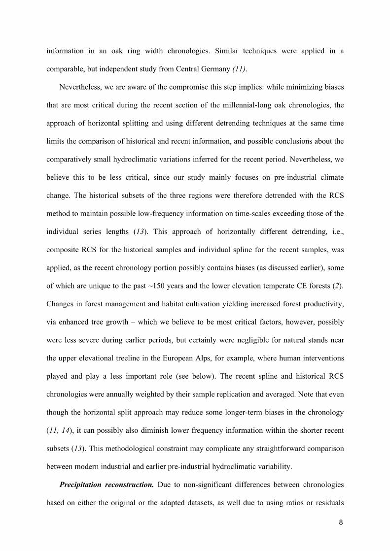
Fig. S1. Series replication of the three historical oak datasets (NEF, SEG, NEG),
using either their original or adaptation subsets (see table S1 and figure S7 for
details).
12
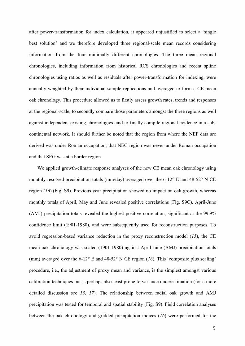
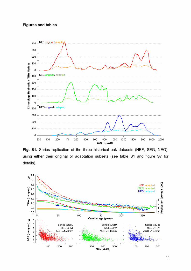
Fig. S2. (A) Regional Curves of the age-aligned TRW measurement series and their
replication using the original and adapted regional sub-sets (see table S1 for details).
(B) Relationship between average growth rate (AGR) and mean segment length
(MSL) of the 7284 oak samples geographically divided into the three regional sub-
sets (Northeast France = NEF, Southeast Germany = SEG, Northeast Germany =
NEG).
Fig. S3. Moving 31-year standard deviations of the three regional high-frequency
chronologies (after 20-year spline detrending with and without power-transformation
and using the original and adapted subsets) before (black) and after (color) variance
stabilization.
13
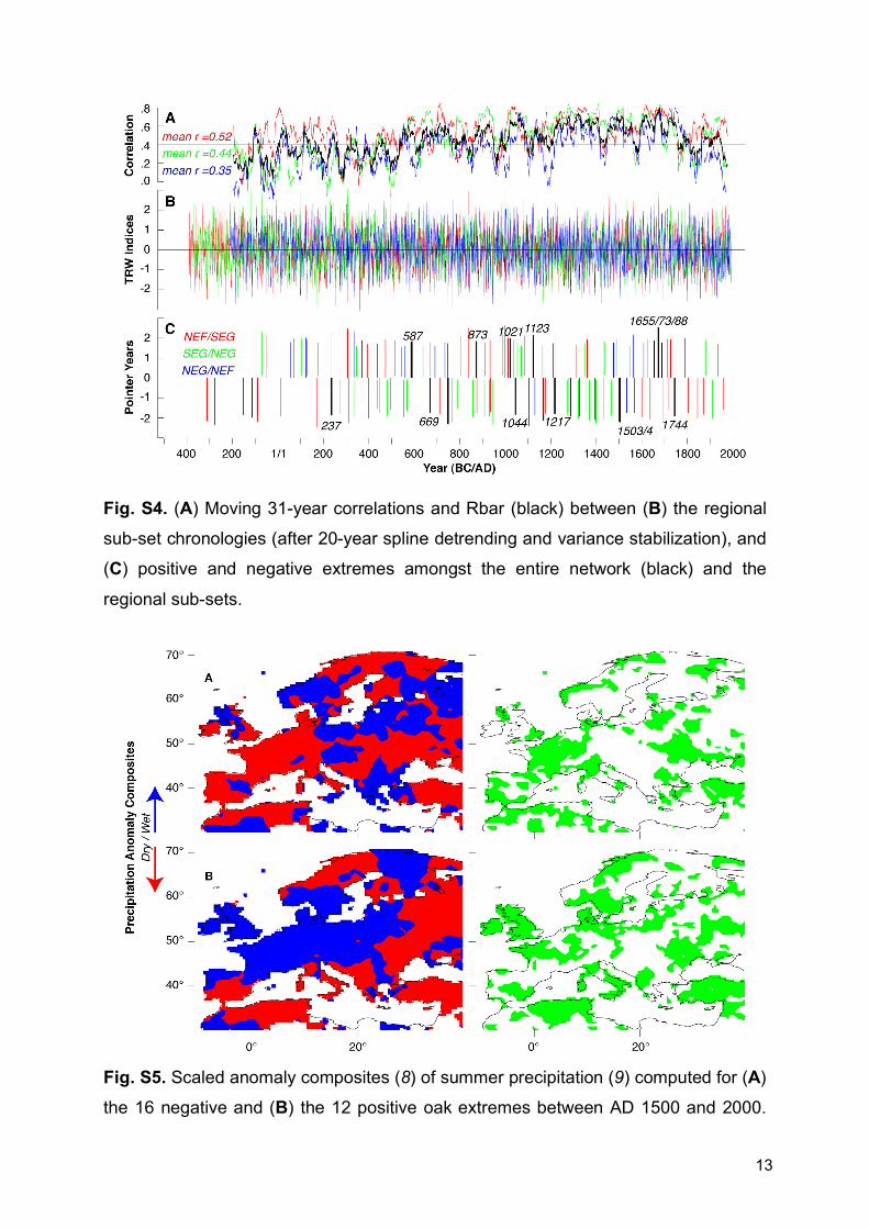
Fig. S4. (A) Moving 31-year correlations and Rbar (black) between (B) the regional
sub-set chronologies (after 20-year spline detrending and variance stabilization), and
(C) positive and negative extremes amongst the entire network (black) and the
regional sub-sets.
Fig. S5. Scaled anomaly composites (8) of summer precipitation (9) computed for (A)
the 16 negative and (B) the 12 positive oak extremes between AD 1500 and 2000.
14
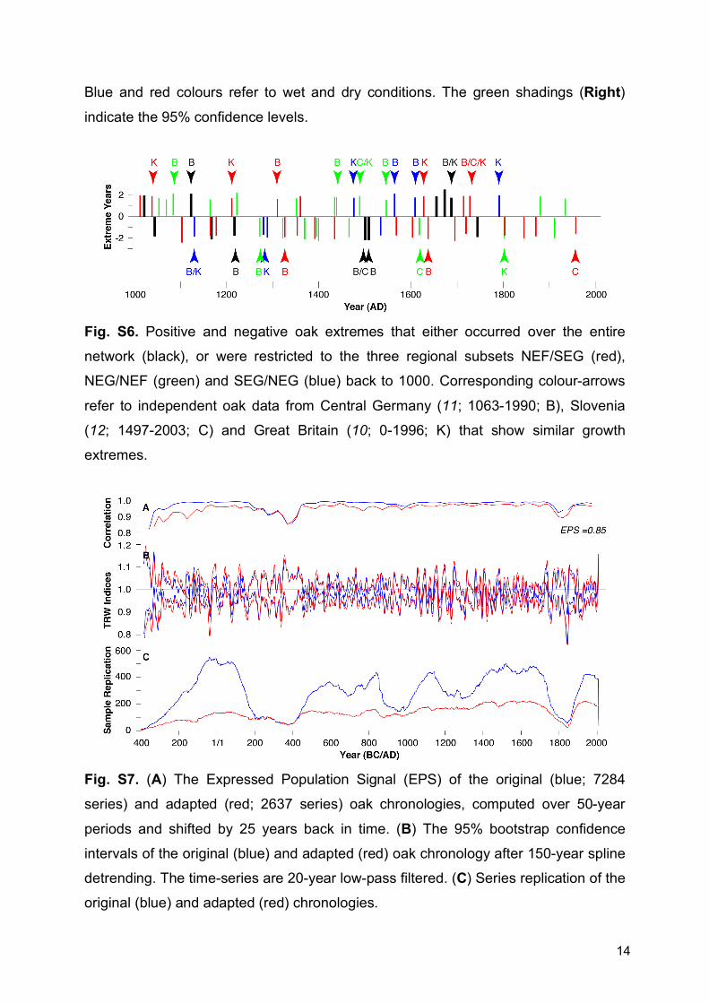
Blue and red colours refer to wet and dry conditions. The green shadings (Right)
indicate the 95% confidence levels.
Fig. S6. Positive and negative oak extremes that either occurred over the entire
network (black), or were restricted to the three regional subsets NEF/SEG (red),
NEG/NEF (green) and SEG/NEG (blue) back to 1000. Corresponding colour-arrows
refer to independent oak data from Central Germany (11; 1063-1990; B), Slovenia
(12; 1497-2003; C) and Great Britain (10; 0-1996; K) that show similar growth
extremes.
Fig. S7. (A) The Expressed Population Signal (EPS) of the original (blue; 7284
series) and adapted (red; 2637 series) oak chronologies, computed over 50-year
periods and shifted by 25 years back in time. (B) The 95% bootstrap confidence
intervals of the original (blue) and adapted (red) oak chronology after 150-year spline
detrending. The time-series are 20-year low-pass filtered. (C) Series replication of the
original (blue) and adapted (red) chronologies.

15
Fig. S8. (A) Precipitation anomalies (mm/day with respect to 1961-1990; CRUTS3)
averaged over the 6-12° E and 48-52° N CE region, compared with different
chronology versions of the three regional subsets: (B) NEF, (C) SEG and (D) NEG.
The light colors refer to four RCS chronologies (ratios/original; residuals/original;
ratios/adapted; residuals/adapted) that allow trend biases to occur, whereas the
bright colors refer to the corresponding four chronology versions after 150-year spline
chronologies that prevent possible biases during the recent time-series ends.

16
Fig. S9. (A) Moving 31-year correlations between AMJ precipitation (averaged over
6-12° E and 48-52° N) and the mean CE oak chronology. (B) Measured (blue) and
reconstructed (green) AMJ precipitation anomalies (mm/day with respect to 1961-
1990; CRUTS3) after scaling over the 1901-1980 period. (C) Correlations between
monthly precipitation totals and the oak chronology (1901-1980), and (D) spatial
spearman correlations of the oak chronology against gridded (0.5°x0.5°) AMJ
precipitation anomalies. The right map shows spatial correlations of the mean of
three instrumental stations (Nancy, Regensburg, Potsdam) best representing the oak
sub-regions against gridded (0.5°x0.5°) AMJ precipitation anomalies.
Fig. S10. Temporal distribution of the 1546 Alpine conifer ring width series from the
Austrian Alps, classified into recent, historical and sub-fossil material, which have
been used to reconstruct JJA temperature variability.
17
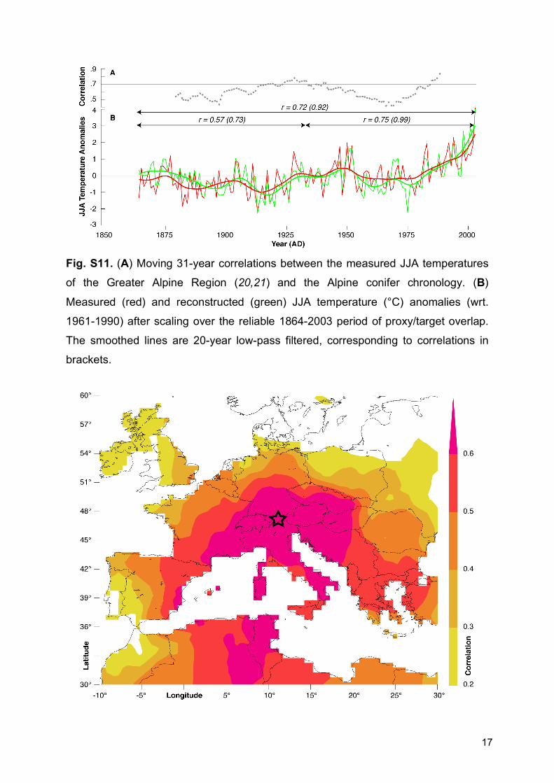
Fig. S11. (A) Moving 31-year correlations between the measured JJA temperatures
of the Greater Alpine Region (20,21) and the Alpine conifer chronology. (B)
Measured (red) and reconstructed (green) JJA temperature (°C) anomalies (wrt.
1961-1990) after scaling over the reliable 1864-2003 period of proxy/target overlap.
The smoothed lines are 20-year low-pass filtered, corresponding to correlations in
brackets.
18
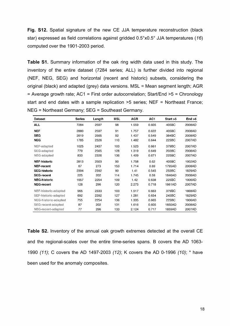
Fig. S12. Spatial signature of the new CE JJA temperature reconstruction (black
star) expressed as field correlations against gridded 0.5°x0.5° JJA temperatures (16)
computed over the 1901-2003 period.
Table S1. Summary information of the oak ring width data used in this study. The
inventory of the entire dataset (7284 series; ALL) is further divided into regional
(NEF, NEG, SEG) and horizontal (recent and historic) subsets, considering the
original (black) and adapted (grey) data versions. MSL = Mean segment length; AGR
= Average growth rate; AC1 = First order autocorrelation; Start/End >5 = Chronology
start and end dates with a sample replication >5 series; NEF = Northeast France;
NEG = Northeast Germany; SEG = Southeast Germany.
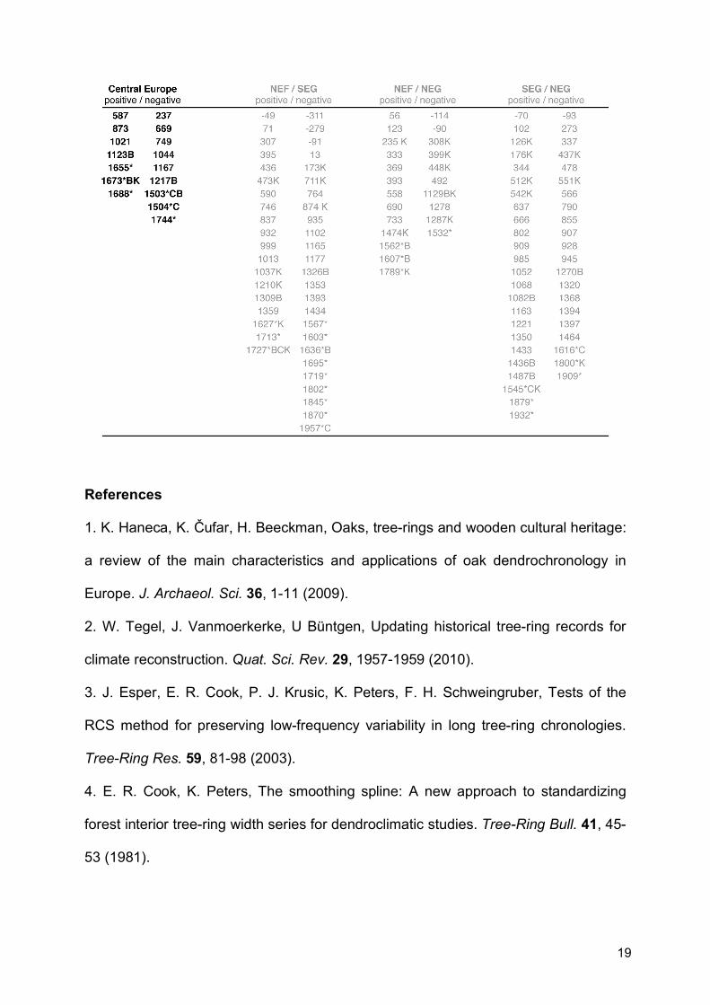
Table S2. Inventory of the annual oak growth extremes detected at the overall CE
and the regional-scales over the entire time-series spans. B covers the AD 1063-
1990 (11); C covers the AD 1497-2003 (12); K covers the AD 0-1996 (10); * have
been used for the anomaly composites.
19
References
1. K. Haneca, K. Čufar, H. Beeckman, Oaks, tree-rings and wooden cultural heritage:
a review of the main characteristics and applications of oak dendrochronology in
Europe. J. Archaeol. Sci. 36, 1-11 (2009).
2. W. Tegel, J. Vanmoerkerke, U Büntgen, Updating historical tree-ring records for
climate reconstruction. Quat. Sci. Rev. 29, 1957-1959 (2010).
3. J. Esper, E. R. Cook, P. J. Krusic, K. Peters, F. H. Schweingruber, Tests of the
RCS method for preserving low-frequency variability in long tree-ring chronologies.
Tree-Ring Res. 59, 81-98 (2003).
4. E. R. Cook, K. Peters, The smoothing spline: A new approach to standardizing
forest interior tree-ring width series for dendroclimatic studies. Tree-Ring Bull. 41, 45-
53 (1981).

20
5. G. Battipaglia, et al., Five centuries of Central European temperature extremes
reconstructed from tree-ring density and documentary evidence. Glob. Planet.
Change 72, 182-191 (2010).
6. E. R. Cook, K. Peters, Calculating unbiased tree-ring indices for the study of
climatic and environmental change. Holocene 7, 361-370 (1997).
7. D. Frank, J. Esper, E. R. Cook, Adjustment for proxy number and coherence in a
large-scale temperature reconstruction. Geophys. Res. Lett. 34, doi:
10.1029/2007GL030571 (2007).
8. T. J. Brown, B. L. Hall, The use of t values in climatological composite analyses. J.
Clim. 12, 2941-2945 (1999).
9. A. Pauling, J. Luterbacher, C. Casty, H. Wanner, 500 years of gridded high-
resolution precipitation reconstructions over Europe and the connection to large-
scale circulation. Clim. Dyn. 26, 387-405 (2006).
10. P. M. Kelly, H. H. Leuschner, K. R. Briffa, I. C. Harris, The climatic interpretation
of pan-European signature years in oak ring-width series. Holocene 12, 689-694
(2002).
11. U. Büntgen, et al., Tree-ring indicators of German summer drought over the last
millennium. Quat. Sci. Rev. 29, 1005-1016 (2010).
12. K. Čufar, M. De Luis, D. Eckstein, L. Kajfez-Bogataj, Reconstructing dry and wet
summers in SE Slovenia from oak tree-ring series. Int. J. Biometeorol. 52, 607-615
(2008).
13. E. R. Cook, K. R. Briffa, D. M. Meko, D. A. Graybill, G. Funkhouser, The
‘segment length curse’ in long tree-ring chronology development for palaeoclimatic
studies. Holocene 5, 229-237 (1995).
14. U. Büntgen, J. Esper, D. C. Frank, K. Nicolussi, M. Schmidhalter, A 1052-year
tree-ring proxy for Alpine summer temperatures. Clim. Dyn. 25, 141-153 (2005).
21
15. J. Esper, D. C. Frank, R. J. S. Wilson, K. R. Briffa, Effect of scaling and
regression on reconstructed temperature amplitude for the past millennium.
Geophys. Res. Lett. 32, doi: 10.1029/2004GL021236 (2005).
16. T. D. Mitchell, P. D. Jones, An improved method of constructing a database of
monthly climate observations and associated high-resolution grids. Int. J. Climatol.
25, 693-712 (2005).
17. D. C. Frank, et al., Ensemble reconstruction constraints of the global carbon
cycle sensitivity to climate. Nature 463, 527-530 (2010).
18. K. Nicolussi, et al., A 9111 year long conifer tree-ring chronology for the
European Alps: a base for environmental and climatic investigations. Holocene 19,
909-920 (2009).
19. I. Auer, et al., HISTALP – Historical instrumental climatological surface time
series of the greater Alpine region 1760-2003. Int. J. Climatol. 27, 17-46 (2007).
20. R. Böhm, et al., The early instrumental warm-bias: a solution for long central
European temperature series 1760–2007. Clim. Change 101, 41-67 (2010).
21. U. Büntgen, D. C. Frank, D. Nievergelt, J. Esper, Summer temperature variations
in the European Alps, AD 755-2004. J. Clim. 19, 5606-5623 (2006).
22. U. Büntgen, et al., Assessing the spatial signature of European climate
reconstructions. Clim. Res. 41, 125-130 (2010).