REPRESENTATION OF PROBABILITY DENSITY FUNCTIONS FROM ORBITDETERMINATION USING THE PARTICLE FILTER

Alinda K. Mashiku(1), James Garrison(2), and J. Russell Carpenter(3)

(1)(2)Purdue University, 701 W. Stadium Ave, West Lafayette, IN 47906,(765-496-2396,765-496-7482), (aaligawe, jgarriso@purdue.edu)

(3)NASA Goddard Space Flight Center, Greenbelt, MD 20771, 301-286-7526,james.r.carpenter@nasa.gov

Abstract: Statistical orbit determination enables us to obtain estimates of the state and thestatistical information of its region of uncertainty. In order to obtain an accurate representation ofthe probability density function (PDF) that incorporates higher order statistical information, wepropose the use of nonlinear estimation methods such as the Particle Filter. The Particle Filter (PF)is capable of providing a PDF representation of the state estimates whose accuracy is dependent onthe number of particles or samples used. For this method to be applicable to real case scenarios,we need a way of accurately representing the PDF in a compressed manner with little informationloss. Hence we propose using the Independent Component Analysis (ICA) as a non-Gaussiandimensional reduction method that is capable of maintaining higher order statistical informationobtained using the PF. Methods such as the Principal Component Analysis (PCA) are based onutilizing up to second order statistics, hence will not suffice in maintaining maximum informationcontent. Both the PCA and the ICA are applied to two scenarios that involve a highly eccentricorbit with a lower apriori uncertainty covariance and a less eccentric orbit with a higher a prioriuncertainty covariance, to illustrate the capability of the ICA in relation to the PCA.

Keywords: Orbit Determination, Particle Filter, Non-Gaussian, Data Compression, NonlinearEstimation.

1. Introduction

The Statistical Orbit Determination (OD) problem involves the estimation of the states of a spaceobject based on noisy measurements. In recent years, there has been a dramatic increase of spaceobjects (assets and space debris) particularly in Low Earth Orbit (LEO) [?]. This increase of spaceobjects pose a threat to the space assets based on potential collisions as well as the increase inoperational costs during maneuvers required to avoid collisions. For instance, in 2009, CelesTrakpredicted that an Iridium Satellite and the defunct Russian Satellite Cosmos, would have a closeapproach of 584 meters [?, ?], nevertheless they collided with one another. Since 1998, the ISS hasperformed 13 maneuvers to avoid collisions with space debris [?]. The last maneuver was in 2009,performed to avoid the debris from the Iridium and Cosmos satellite collisions. This required 30hours to plan and execute [?] as well as the cost of propellant for the delta-V maneuver implemented.The classical methods of statistical OD, such as the Extended Kalman Filter (EKF) [?] and theUnscented Kalman Filter (UKF) [?], may not always be the best choice of an estimator for allproblems because they only consider the second moments of the state. As long as the observationerror and process noise can be accurately assumed to have a Gaussian distribution, these secondmoments are sufficient to infer all other statistics as well. One example in which the non-Gaussianerrors could arise is when observations are based upon short arcs of tracking data when tracking

1

https://ntrs.nasa.gov/search.jsp?R=20120017458 2018-05-24T00:59:05+00:00Z

orbit debris. Hence, an accurate prediction of the states over longer durations of time is imperativefor such tracking and collision avoidance applications.

A good prediction of not only the mean state, but also the shape of the state distribution is importantfor the orbit debris problem, since even events with very low probabilities are of concern. Toaccurately predict the likelihood of these low-probability events, we must accurately predict thetails of the distribution. Given that the orbit dynamics are non-linear, even if the a priori state vectorhas a Gaussian distribution, propagation with non-linear dynamics would evolve this distributioninto a non-Gaussian one. In addition to predicting the state distribution, there also needs to be amethod of numerically representing this distribution in order to generate a catalog of all orbitingobjects for predicting the likelihood of possible collisions. At present, orbit catalogs use somedefinition of a common ephemerides, for example the NORAD Two-line elements ephemerides,which only represent the mean orbit state, providing no information on its probability distribution.Development of Nonlinear filtering techniques capable of predicting the state distribution (a fullProbability Density Function (PDF)), are necessary to address this type of problem. The ParticleFilter algorithm (PF) is used as a nonlinear filtering technique, based on a sequential Monte Carloapproach representing the required state PDF by a set of random samples or particles. The accuracyof the prediction and estimation of the states increases with the increase in the number of particles.

Having developed a method for predicting the state PDF, it is then necessary to derive a compactform for storing and distributing the distribution. Representing the state PDF of an orbit witha large number of particles is not a practical method for storing or distributing orbit state data.The objective of this work, therefore, is to develop new methods for representing the full PDFof the orbit state, in a compact data record which could be distributed much in the same way asephemerides are used today. We will approach this problem by investigating methods to decorrelatethe the state into independent uni- or multi-variate components, whose PDFs could be morecompactly represented. For example, some components of the decorrelated PDF might be accuratelyrepresented by many fewer particles than the original state PDF, or might be easier to approximatewith continuous functions using methods such as the wavelet transform, characteristic functions,and/or kernel densities. Conventional methods that perform orthogonal transformations to obtainlinearly uncorrelated variables, such as the Principal Component Analysis (PCA), would loseinformation present in the higher moments if the distribution is not Gaussian. In this paper, we willapply a method known as the Independent Component Analysis (ICA) [?, ?, ?, ?] method, which iscapable of decorrelating non-Gaussian data by finding the local extrema of the kurtosis (fourth ordermoment) of a linear combination of the states and thus estimating the non-Gaussian independentcomponents.

Methods such as PCA and ICA may also offer additional compression from dimensional reduction insome cases. For example, the OD process may require the augmentation of the state with additionalcomponents that are not strongly correlated with the minimal subset of components required foraccurate state prediction. PCA and ICA would be expected to assign relatively lower eigenvaluesto components arising from such states, identifying them as good candidates for elimination.Furthermore, the OD process may use a state vector whose coordinate representation is well-suitedto OD, but less suitable for long-term propagation. The transformation of coordinates inherent inPCA and ICA may help to identify alternative representations, analogous to orbital elements, which

2

have a simpler PDF structure, and hence be more easily predicted.

To demonstrate our approach, we apply ICA and PCA to both decorrelate and dimensionally reduceCartesian particle representations of the PDF of a two-body orbit. Since out-of-plane motion insuch orbits is known to be decoupled from in-plane motion, we anticipate a dimensional reductionfrom 6 states to 4 may reasonably approximate the most strongly non-Gaussian components ofthe PDF. We will show that the resulting compression of the original 6-dimensional Cartesian setof 1000 particles can be used to accurately reconstruct the original PDF, at the epoch at whichwe perform the translation. The ability of the compressed representation to form the basis for anaccurate prediction is the topic of ongoing work, and will not be addressed in this paper.

This paper is organized into eight sections. Section 1 covers the introduction, section 2 describesthe Particle Filter algorithm. In sections 3 and 4, the methods of dimensional reduction and theproblem description are presented. The results are presented in section 5 and the conclusion andfuture work are presented in section 6. Section 7 will constitute the acknowledgements and thereferences are listed in section 8.

2. Particle Filter

In order to incorporate the higher order moments of the state and measurement errors, we needto be able to study the evolution of the full state PDF in the OD process. The Particle Filter (PF)is a simulation-based filter based on the sequential Monte Carlo approach, effective in estimatingthe full state PDF of nonlinear models or non-Gaussian PDFs [?, ?, ?]. The central idea of a PF isto represent the required probability density function (PDF) by a set of N >> 1 random samples

known as particles {X(i)k }

N

i=1, with associated weights {w(i)k }N

i=1, such that

p(Xk|Yk)≈N∑

i=1w(i)

k δ (Xk−X(i)k ) (1)

where the particles are identically and independently distributed (i.i.d) samples drawn from theinitial PDF with an initial Gaussian distribution assumption. The weights are the probability valuesthat are the approximations of the relative densities of the particles such that their sum equals one[?, ?, ?]. The state estimate is given as a conditional density called the posterior density p(Xk|Yk).Estimators based on this posterior density are constructed from Bayes’ theorem, which is defined as

p(X|Y) =p(Y|X)p(X)

p(Y)(2)

where p(X) is called the prior density (before measurement), p(Y|X)is called the likelihood andp(Y)is called the evidence (normalizes the posterior to assure the integral sums up to unity) [?, ?].In the execution of the general PF algorithm, a common effect ensues where the variance of theweights increases over time. This phenomenon is known as sampling degeneracy, in that there is aninsufficient number of effective particles required to fully capture the PDF. A way of overcomingthe sampling degeneracy is to derive the importance distribution that minimizes the variance of thedistribution of the weights. The corresponding weights are given by:

wk = wk−1 p(Yk|Xk−1) (3)

3

wk = wk−1

∫p(Yk|Xk)p(Xk|Xk−1)dXk (4)

This means that the weights can be calculated before the particles are propagated to time k. Fromthe equations above, we see that there is a problem in the sense that the evaluation of the integralgenerally does not have an analytic form and that the particles’ weight updates are based on theknowledge of the state at the past time step and the current measurement only i.e. p(Xk|Xk−1,Yk).So, a reasonable choice for the importance distribution is the transition prior p(Xk|Xk−1)[?].

2.1. PF Algorithm

Let Xk = (X0,X1, ...,Xk) and Yk = (Y0,Y1, ...Yk) be the stacked vectors of states and observationsup to time k and {wi

k, i = 1,2, ...,N} represent the weights of the N particles at each time k. Theestimation process can be sectioned into three parts: initialization, time update or prediction and themeasurement update. Each step is described below for the PF implementation.

1. Initialization at k = 0, for i = 1,...,N• Sample N particles from the prior Xi

0 ∼ p(X0)• Calculate the weights of the particles from the initial distribution (assume Gaussian)

wi0 = p(Y0|Xi

0)

• Normalize the weights wi0 =

wi0

wTusing total weight wT =

∑Ni wi

02. Time Update or Prediction at k ≥ 1, for i = 1,...,N

• Predict the particles through the dynamics

Xik = f (Xi

k−1)+ vk (5)

p(Xk|Yk−1) =∫

p(Xk|Xk−1)p(Xk−1|Yk−1)dXk−1 (6)

3. Measurement Update• Update the weights using the innovation from the measurements assuming that the

measurements are Gaussian distributed

wik = wi

k−1p(Yk|Xi

k)p(Xik|Xi

k−1)

q(Xik|X i

k−1,Yk)(7)

• We assume that the importance distribution q(Xik|X i

k−1,Yk) in this case is equal to theprior density p(Xi

k|Xik−1) [?], so that,

wik = wi

k−1× p(Yk|Xik) (8)

• Normalize the weights wik =

wik

wTusing total weight wT =

∑Ni wi

k

• The final posterior density estimate p(Xk|Yk) =∑N

i=1 w(i)k δ (Xk−X(i)

k )

Due to the fact that the prior density is usually broader than the likelihood, only a few particleswill be assigned higher weight during the measurement update step causing sampling degeneracy.The solution to overcome sampling degeneracy is to resample the particles. Let Ne f f denote theeffective sample size, which can be estimated by [?, ?]: N̂e f f =

1∑i(w

ik)

2 . Also let Nth denote a lower

4

threshold for the effective sample size, which is arbitrarily chosen with respect to the accuracydesired; the larger the threshold, the more accurate the PDF results and the more computational costincurred.

If Ne f f > Nth, then the sampling degeneracy is not low enough, the filter continues on to step 2 forthe next time update. Otherwise, we replicate the particle with the highest weight to replace theparticles falling below the threshold and then renormalize the weights. However, resampling doeshave its own shortcomings, since the particles that have higher weights are statistically selectedeach time thus losing the diversity of the samples. This loss of diversity may also cause divergenceof the estimates. To avoid the loss of diversity the replicated particles are “jittered/spread-out” byadding process noise to spread the resampled particles [?, ?].

3. Decorrelation, Scaling, and Dimensional Reduction

The PF requires the implementation of a large number particles to achieve a good PDF representation.In addition, the computational and data allocation costs compound with increase in both the numberof particles and the dimension of the state. We propose to compress the data with respect to thedimensional size and the number of particles used. However, since our data does not possess aGaussian distribution, conventional methods that perform orthogonal transformations to obtainlinearly uncorrelated variables, such as the principal component analysis, will contribute to theloss of information present in the higher moments. Hence, we propose to apply the method ofIndependent Component Analysis (ICA). ICA has been developed to be capable of decorrelatingnon-Gaussian data by finding the local extrema of the kurtosis (fourth order moment) of a linearcombination of the states and thus providing the non-Gaussian mutually independent components[?, ?, ?].

Since the states have different scaling in order of magnitudes (i.e. position vs velocity), we normalizethe particles for our states based on the canonical units. For distance, we scale the value by thedistance unit (1 DU⊕) which is equivalent to the value of the radius of the Earth (6378.145km). Forvelocity, the scaling metric is given as the distance unit/ time unit (1 DU⊕/TU⊕) of equivalency7.90536828 km/s [?]. The implementation of the scaling will help to ensure an equal weighting ofinformation from the velocities that are typically of lower magnitudes.

As an introduction to ICA, we will first review Principal Component Analysis (PCA), commonlyused to decorrelate data with a Gaussian distribution.

3.1. Principal Component Analysis

Principal Component Analysis (PCA) is the orthogonal transformation of a set of possibly correlateddata into a set of linearly uncorrelated variables known as the principal components [?, ?]. In otherwords, PCA finds a smaller set of variables with less redundancy [?]. The number of the principalcomponents obtained are usually equal to or less than the dimension of the original data set.The component with the largest variance is deemed as the first component and each succeedingcomponent with a higher variance is computed in that order under the constraint that it be orthogonalto the preceding components [?, ?].

5

The principal components are obtained by first centering the data set (i.e. state particles Xik) and

subtracting its mean to obtain the standardized data set x̃ik

x̃ik = Xi

k−E[Xik] (9)

The eigenvectors V corresponding to the decreasing eigenvalues D, represent the direction of thecomponents in order of their decreasing variances.

Cx̃x̃ = E{x̃x̃T} (10)D = V−1Cx̃x̃V (11)

In PCA, the components with negligible collective eigenvalues can be considered as redundant orpertaining to negligible information. Thus, the principal components kept are in reference to thedirections with the maximum variance and are considered sufficient to represent the original data ina new coordinate frame within a reasonable level of accuracy.

The shortcomings of using the PCA for a non-Gaussian distributed data is that the principalcomponents computed are based on the covariance matrix, which only incorporates second ordermoments statistics. Hence using the principal components obtained by PCA defeats the purpose ofimplementing the PF to obtain the non-Gaussian distributed particles of our state estimates.

3.2. Independent Component Analysis

Independent Component Analysis (ICA) is a signal processing technique that is used to representa set of random variables as linear combinations of statistically independent component variables[?, ?, ?, ?, ?, ?]. The most common demonstration of the application of the ICA is known as the‘cocktail party problem’. Given a room with three people speaking at the same time to an audienceand three microphones recording the mixture of the three speech signals x1(t),x2(t), and x3(t). Eachof these recored signals can be represented as a weighted sum of the speech signals emitted by thethree speakers, denoted by s1(t),s2(t), and s3(t). This is expressed as a linear equation:

x1(t) = a11s1(t)+a12s2(t)+a13s3(t) (12)x2(t) = a21s1(t)+a22s2(t)+a23s3(t) (13)x3(t) = a31s1(t)+a32s2(t)+a33s3(t) (14)

where ai j with i, j = 1, . . .3 are some parameters that depend on the distances of the microphonesfrom the speakers [?, ?]. It would be easy to solve for the speech signals s1(t),s2(t), and s3(t) if weknew ai j, but neither of them are known. However, if we can assume that the signals s1(t),s2(t),and s3(t) are statistically independent at each time instant t, we can use ICA to solve for ai j and inturn solve for s1(t),s2(t), and s3(t).

Beyond the assumption that the signals are statistically independent, the independent componentsmust have non-Gaussian distributions in order for higher order cumulants or moments to be usefulin the estimation of the independent components [?, ?]. For Gaussian distributions, the higher ordermoments are zero. Given that our state estimates using the PF are non-Gaussian, we expect somebenefit from implementing the ICA for state decorrelation and dimensional reduction.

6

Given that at a time k we have an estimated a state vector Xi of dimension-N, with m particlesXi = (X1,X2, . . .Xm), we form a linear combination of S-dimensional independent variables s j =(s1,s2, . . .sm), where S≤ N; we then compute a mixing matrix A(N×S), such that

X = As (15)

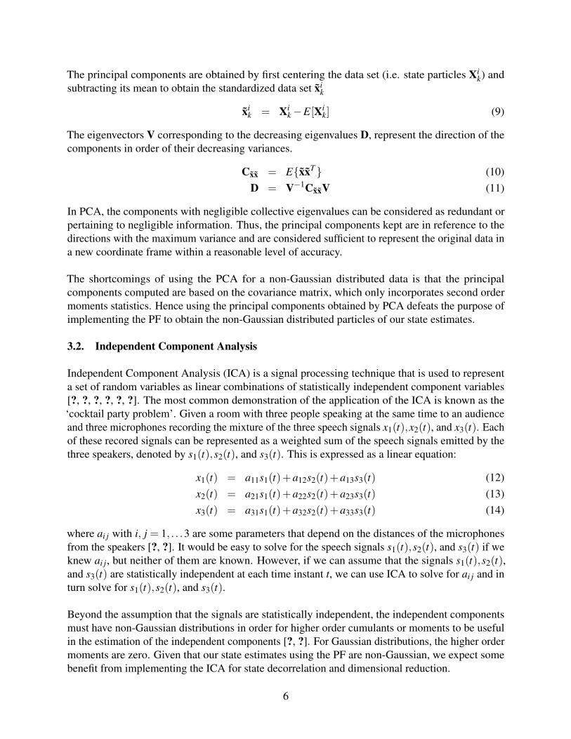
where ∀ j,sj has unit variance. The data X is pre-whitened to obtain a new set of data x = MXthat is uncorrelated and has a unit variance, with M known as the whitening matrix. We computethe orthonormal matrix B whose columns w1,w2, . . .ws are in the direction of the maximum orminimum kurtosis of x (see Fig. 1).

kurt(wT x) = E{(wT x)4}−3[E{(wT x)2}]2 (16)= E{(wT x)4}−3||w||4 (17)

The columns w1,w2, . . .ws are solved using the objective function J (w) under the constraint that||w||= 1,

J (w) = E{(wT x)4}−3||w||4 +F(||w||2) (18)

where F is a penalty term due to the constraint. In order to solve for the columns w1,w2, . . .ws,rapidly, a fixed-point iteration scheme is generated by taking the expectation of Eq. 18, equating itto zero and normalizing the penalty term. We obtain

w = α× (E{x(wT x)3}−3||w||2w) (19)

where α is an arbitrary scalar that diffuses under the normalizing constraint of w.

Hence, the fixed-point iteration scheme is implemented as follows:1. Take a random initial vector w(0) or norm 1. Let k = 1.2. Let w(k) = E{x(w(k−1)T x)3}−3w(k−1).3. Divide w(k) by its norm4. If |w(k)T w(k−1)| is not close enough to 1, let k = k+1 and go back to step 2, or else output

vector w1, and continue until ws is obtained.

The basic idea is that we search for the vector w of norm 1, such that the linear combination of wT x,has maximum or minimum kurtosis. That will give us the independent components s [?]. Moreover,the number of the independent components desired is declared beforehand, hence the search for thecolumns of the matrix B, is maximized based on the stated number of independent components.

A detailed description of the algorithm implementation can be found in references [?, ?]. Hence,our independent components s are given by

x = MX = MAs (20)B = MA (21)s = BTx (22)

One ambiguity in the ICA method is that the order of the independent components is indeterminate.Because both A and s are unknown, the order of the sums in Eq. 12, Eq. 13 and Eq. 14, canbe interchanged and hence any independent component can be called the first one [?]. For ourapplication, this is not a hindrance since our goal is to obtain the independent components that aredimensionally reduced and that could be compressed univariately or bivariately.

7

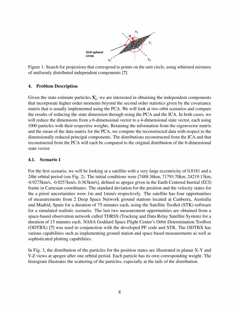
Figure 1. Search for projections that correspond to points on the unit circle, using whitened mixturesof uniformly distributed independent components [?]

4. Problem Description

Given the state estimate particles Xik, we are interested in obtaining the independent components

that incorporate higher order moments beyond the second order statistics given by the covariancematrix that is usually implemented using the PCA. We will look at two orbit scenarios and comparethe results of reducing the state dimension through using the PCA and the ICA. In both cases, wewill reduce the dimensions from a 6-dimensional vector to a 4-dimensional state vector, each using1000 particles with their respective weights. Retaining the information from the eigenvector matrixand the mean of the data matrix for the PCA, we compute the reconstructed data with respect to thedimensionally reduced principal components. The distributions reconstructed from the ICA and thatreconstructed from the PCA will each be compared to the original distribution of the 6-dimensionalstate vector.

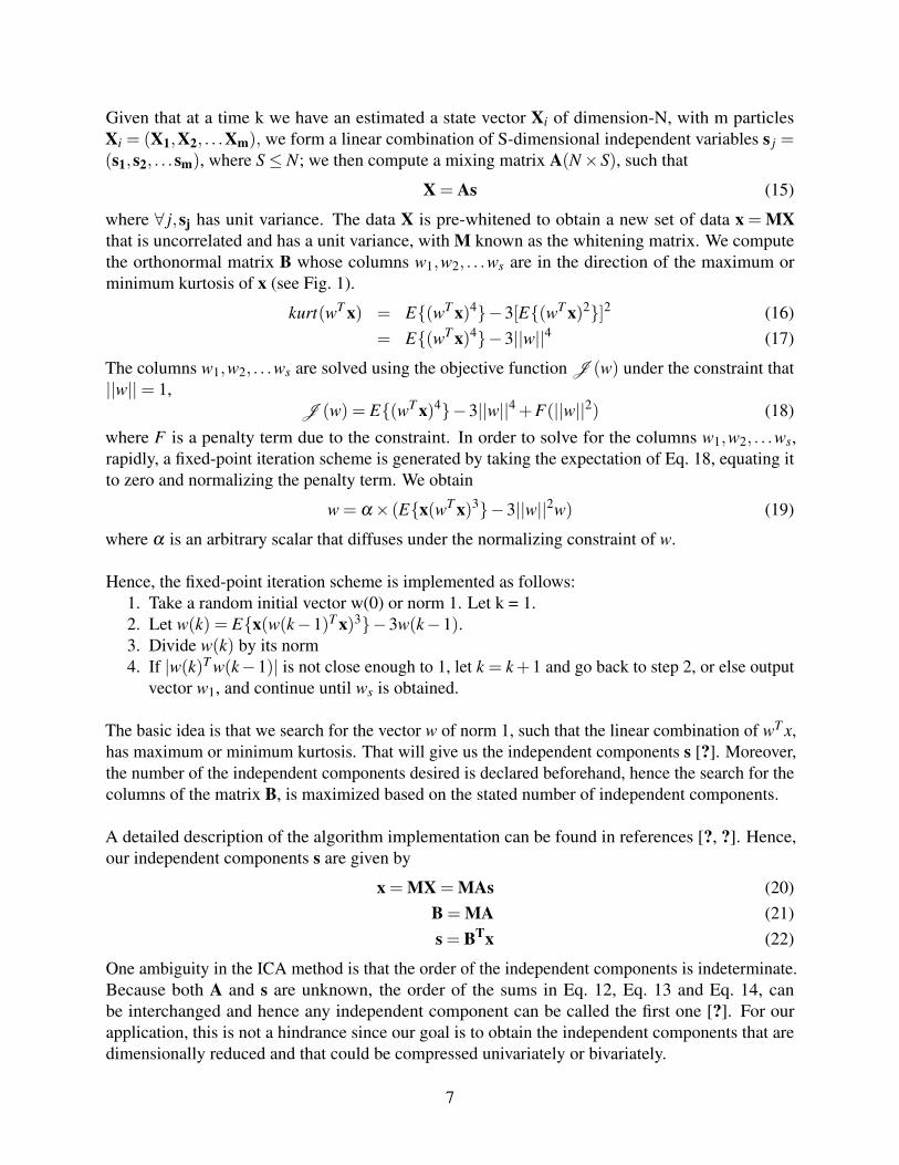
4.1. Scenario 1

For the first scenario, we will be looking at a satellite with a very large eccentricity of 0.8181 and a24hr orbital period (see Fig. 2). The initial conditions were [7488.36km, 71793.70km, 24219.13km,-0.9275km/s, -0.0257km/s, 0.363km/s], defined as apogee given in the Earth Centered Inertial (ECI)frame in Cartesian coordinates. The standard deviation for the position and the velocity states forthe a priori uncertainties were 1m and 1mm/s respectively. The satellite has four opportunitiesof measurements from 2 Deep Space Network ground stations located at Canberra, Australiaand Madrid, Spain for a duration of 75 minutes each, using the Satellite Toolkit (STK) softwarefor a simulated realistic scenario. The last two measurement opportunities are obtained from aspace-based observation network called TDRSS (Tracking and Data Relay Satellite System) for aduration of 15 minutes each. NASA Goddard Space Flight Center’s Orbit Determination Toolbox(ODTBX) [?] was used in conjunction with the developed PF code and STK. The ODTBX hasvarious capabilities such as implementing ground station and space based measurements as well assophisticated plotting capabilities.

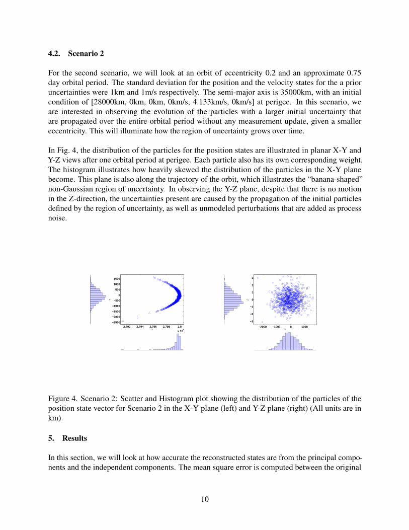
In Fig. 3, the distribution of the particles for the position states are illustrated in planar X-Y andY-Z views at apogee after one orbital period. Each particle has its own corresponding weight. Thehistogram illustrates the scattering of the particles, especially at the tails of the distribution.

8

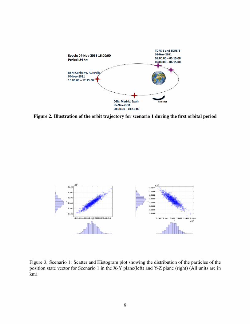
Figure 2. Illustration of the orbit trajectory for scenario 1 during the first orbital period

4844.44844.64844.8 4845 4845.24845.44845.6

7.1462

7.1462

7.1462

7.1463

7.1463

7.1463x 10

4

Y

X7.1462 7.1462 7.1462 7.1463 7.1463 7.1463

x 104

2.5156

2.5156

2.5156

2.5156

2.5156

2.5156

2.5156

2.5156x 10

4

Y

Z

Figure 3. Scenario 1: Scatter and Histogram plot showing the distribution of the particles of theposition state vector for Scenario 1 in the X-Y plane(left) and Y-Z plane (right) (All units are inkm).

9

4.2. Scenario 2

For the second scenario, we will look at an orbit of eccentricity 0.2 and an approximate 0.75day orbital period. The standard deviation for the position and the velocity states for the a prioruncertainties were 1km and 1m/s respectively. The semi-major axis is 35000km, with an initialcondition of [28000km, 0km, 0km, 0km/s, 4.133km/s, 0km/s] at perigee. In this scenario, weare interested in observing the evolution of the particles with a larger initial uncertainty thatare propagated over the entire orbital period without any measurement update, given a smallereccentricity. This will illuminate how the region of uncertainty grows over time.

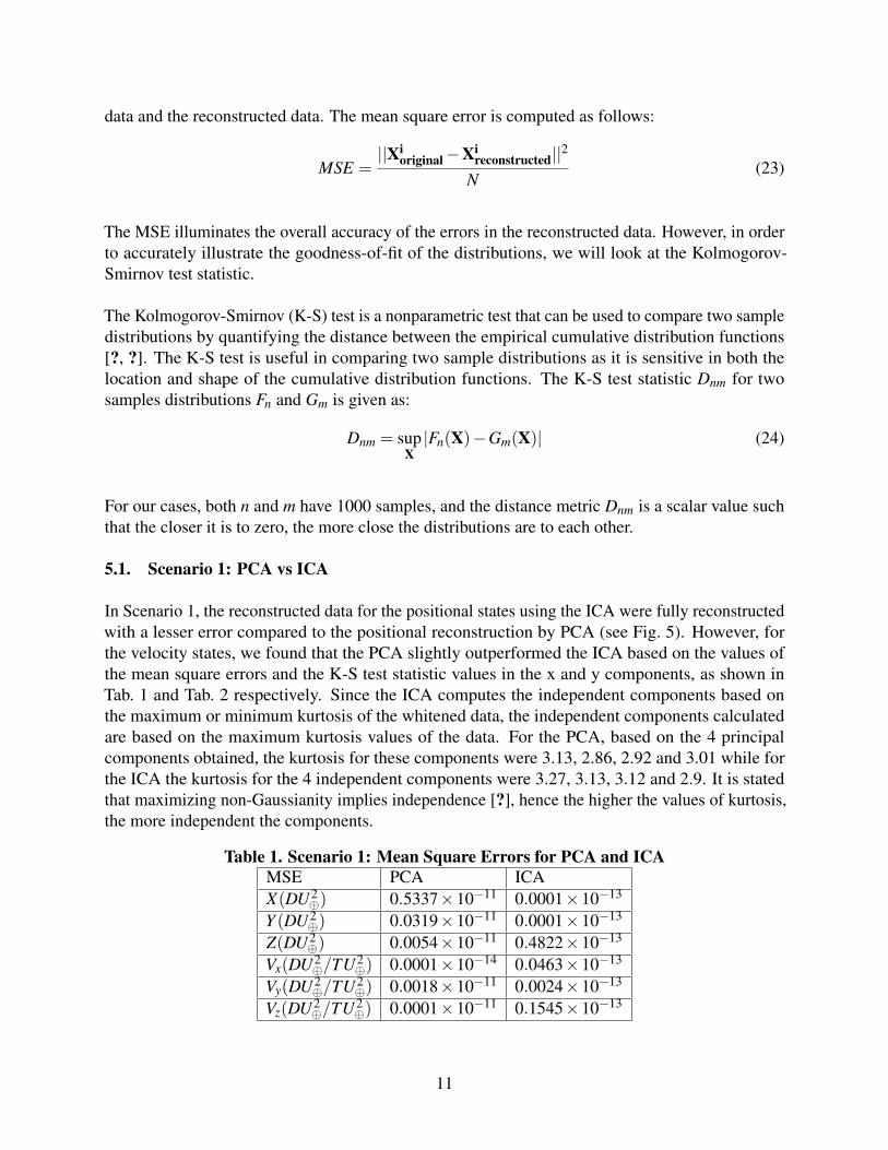
In Fig. 4, the distribution of the particles for the position states are illustrated in planar X-Y andY-Z views after one orbital period at perigee. Each particle also has its own corresponding weight.The histogram illustrates how heavily skewed the distribution of the particles in the X-Y planebecome. This plane is also along the trajectory of the orbit, which illustrates the “banana-shaped”non-Gaussian region of uncertainty. In observing the Y-Z plane, despite that there is no motionin the Z-direction, the uncertainties present are caused by the propagation of the initial particlesdefined by the region of uncertainty, as well as unmodeled perturbations that are added as processnoise.

2.792 2.794 2.796 2.798 2.8

x 104

−2500

−2000

−1500

−1000

−500

0

500

1000

1500

X

Y

−2000 −1000 0 1000

−3

−2

−1

0

1

2

3

Y

Z

Figure 4. Scenario 2: Scatter and Histogram plot showing the distribution of the particles of theposition state vector for Scenario 2 in the X-Y plane (left) and Y-Z plane (right) (All units are inkm).

5. Results

In this section, we will look at how accurate the reconstructed states are from the principal compo-nents and the independent components. The mean square error is computed between the original

10

data and the reconstructed data. The mean square error is computed as follows:

MSE =||Xi

original−Xireconstructed||2

N(23)

The MSE illuminates the overall accuracy of the errors in the reconstructed data. However, in orderto accurately illustrate the goodness-of-fit of the distributions, we will look at the Kolmogorov-Smirnov test statistic.

The Kolmogorov-Smirnov (K-S) test is a nonparametric test that can be used to compare two sampledistributions by quantifying the distance between the empirical cumulative distribution functions[?, ?]. The K-S test is useful in comparing two sample distributions as it is sensitive in both thelocation and shape of the cumulative distribution functions. The K-S test statistic Dnm for twosamples distributions Fn and Gm is given as:

Dnm = supX|Fn(X)−Gm(X)| (24)

For our cases, both n and m have 1000 samples, and the distance metric Dnm is a scalar value suchthat the closer it is to zero, the more close the distributions are to each other.

5.1. Scenario 1: PCA vs ICA

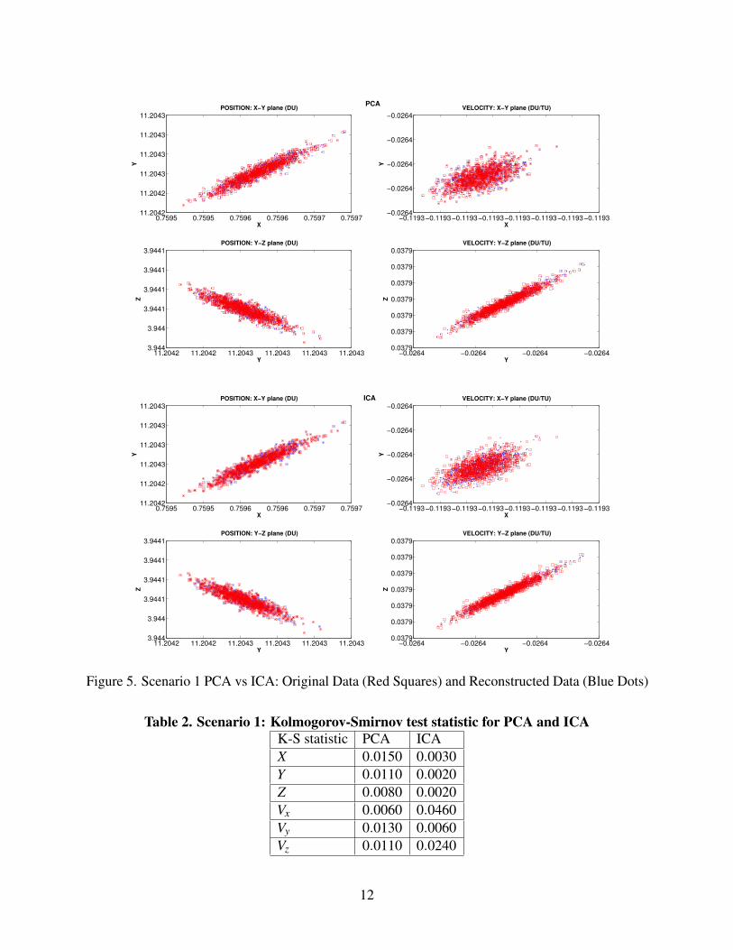
In Scenario 1, the reconstructed data for the positional states using the ICA were fully reconstructedwith a lesser error compared to the positional reconstruction by PCA (see Fig. 5). However, forthe velocity states, we found that the PCA slightly outperformed the ICA based on the values ofthe mean square errors and the K-S test statistic values in the x and y components, as shown inTab. 1 and Tab. 2 respectively. Since the ICA computes the independent components based onthe maximum or minimum kurtosis of the whitened data, the independent components calculatedare based on the maximum kurtosis values of the data. For the PCA, based on the 4 principalcomponents obtained, the kurtosis for these components were 3.13, 2.86, 2.92 and 3.01 while forthe ICA the kurtosis for the 4 independent components were 3.27, 3.13, 3.12 and 2.9. It is statedthat maximizing non-Gaussianity implies independence [?], hence the higher the values of kurtosis,the more independent the components.

Table 1. Scenario 1: Mean Square Errors for PCA and ICAMSE PCA ICAX(DU2

⊕) 0.5337×10−11 0.0001×10−13

Y (DU2⊕) 0.0319×10−11 0.0001×10−13

Z(DU2⊕) 0.0054×10−11 0.4822×10−13

Vx(DU2⊕/TU2

⊕) 0.0001×10−14 0.0463×10−13

Vy(DU2⊕/TU2

⊕) 0.0018×10−11 0.0024×10−13

Vz(DU2⊕/TU2

⊕) 0.0001×10−11 0.1545×10−13

11

0.7595 0.7595 0.7596 0.7596 0.7597 0.759711.2042

11.2042

11.2043

11.2043

11.2043

11.2043

X

Y

POSITION: X−Y plane (DU)

11.2042 11.2042 11.2043 11.2043 11.2043 11.20433.944

3.944

3.9441

3.9441

3.9441

3.9441

Y

Z

POSITION: Y−Z plane (DU)

−0.1193−0.1193−0.1193−0.1193−0.1193−0.1193−0.1193−0.1193−0.0264

−0.0264

−0.0264

−0.0264

−0.0264

X

Y

VELOCITY: X−Y plane (DU/TU)

−0.0264 −0.0264 −0.0264 −0.02640.0379

0.0379

0.0379

0.0379

0.0379

0.0379

0.0379

Y

Z

VELOCITY: Y−Z plane (DU/TU)

PCA

0.7595 0.7595 0.7596 0.7596 0.7597 0.759711.2042

11.2042

11.2043

11.2043

11.2043

11.2043

X

Y

POSITION: X−Y plane (DU)

11.2042 11.2042 11.2043 11.2043 11.2043 11.20433.944

3.944

3.9441

3.9441

3.9441

3.9441

Y

Z

POSITION: Y−Z plane (DU)

−0.1193−0.1193−0.1193−0.1193−0.1193−0.1193−0.1193−0.1193−0.0264

−0.0264

−0.0264

−0.0264

−0.0264

X

Y

VELOCITY: X−Y plane (DU/TU)

−0.0264 −0.0264 −0.0264 −0.02640.0379

0.0379

0.0379

0.0379

0.0379

0.0379

0.0379

Y

Z

VELOCITY: Y−Z plane (DU/TU)

ICA

Figure 5. Scenario 1 PCA vs ICA: Original Data (Red Squares) and Reconstructed Data (Blue Dots)

Table 2. Scenario 1: Kolmogorov-Smirnov test statistic for PCA and ICAK-S statistic PCA ICAX 0.0150 0.0030Y 0.0110 0.0020Z 0.0080 0.0020Vx 0.0060 0.0460Vy 0.0130 0.0060Vz 0.0110 0.0240

12

5.2. Scenario 2: PCA vs ICA

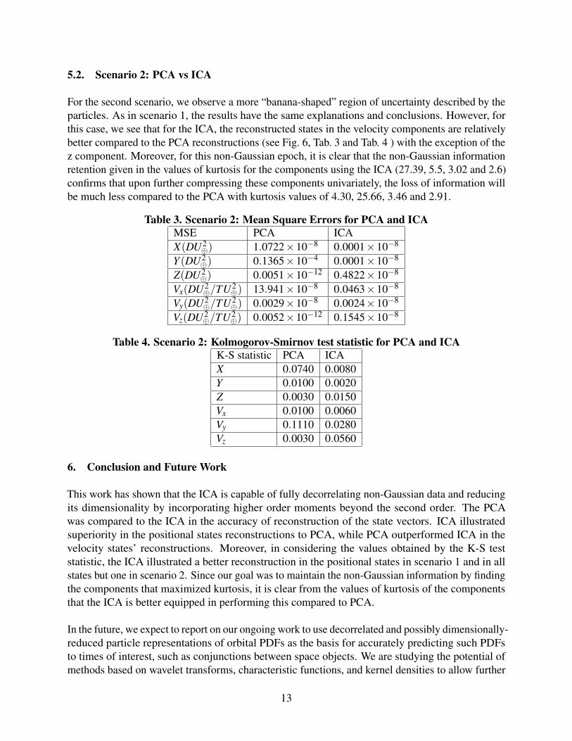
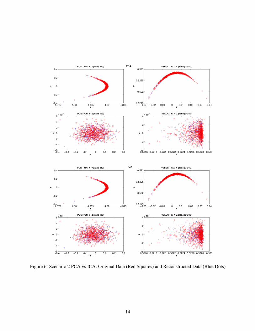
For the second scenario, we observe a more “banana-shaped” region of uncertainty described by theparticles. As in scenario 1, the results have the same explanations and conclusions. However, forthis case, we see that for the ICA, the reconstructed states in the velocity components are relativelybetter compared to the PCA reconstructions (see Fig. 6, Tab. 3 and Tab. 4 ) with the exception of thez component. Moreover, for this non-Gaussian epoch, it is clear that the non-Gaussian informationretention given in the values of kurtosis for the components using the ICA (27.39, 5.5, 3.02 and 2.6)confirms that upon further compressing these components univariately, the loss of information willbe much less compared to the PCA with kurtosis values of 4.30, 25.66, 3.46 and 2.91.

Table 3. Scenario 2: Mean Square Errors for PCA and ICAMSE PCA ICAX(DU2

⊕) 1.0722×10−8 0.0001×10−8

Y (DU2⊕) 0.1365×10−4 0.0001×10−8

Z(DU2⊕) 0.0051×10−12 0.4822×10−8

Vx(DU2⊕/TU2

⊕) 13.941×10−8 0.0463×10−8

Vy(DU2⊕/TU2

⊕) 0.0029×10−8 0.0024×10−8

Vz(DU2⊕/TU2

⊕) 0.0052×10−12 0.1545×10−8

Table 4. Scenario 2: Kolmogorov-Smirnov test statistic for PCA and ICAK-S statistic PCA ICAX 0.0740 0.0080Y 0.0100 0.0020Z 0.0030 0.0150Vx 0.0100 0.0060Vy 0.1110 0.0280Vz 0.0030 0.0560

6. Conclusion and Future Work

This work has shown that the ICA is capable of fully decorrelating non-Gaussian data and reducingits dimensionality by incorporating higher order moments beyond the second order. The PCAwas compared to the ICA in the accuracy of reconstruction of the state vectors. ICA illustratedsuperiority in the positional states reconstructions to PCA, while PCA outperformed ICA in thevelocity states’ reconstructions. Moreover, in considering the values obtained by the K-S teststatistic, the ICA illustrated a better reconstruction in the positional states in scenario 1 and in allstates but one in scenario 2. Since our goal was to maintain the non-Gaussian information by findingthe components that maximized kurtosis, it is clear from the values of kurtosis of the componentsthat the ICA is better equipped in performing this compared to PCA.

In the future, we expect to report on our ongoing work to use decorrelated and possibly dimensionally-reduced particle representations of orbital PDFs as the basis for accurately predicting such PDFsto times of interest, such as conjunctions between space objects. We are studying the potential ofmethods based on wavelet transforms, characteristic functions, and kernel densities to allow further

13

4.375 4.38 4.385 4.39 4.395−0.4

−0.2

0

0.2

0.4

X

Y

POSITION: X−Y plane (DU)

−0.4 −0.3 −0.2 −0.1 0 0.1 0.2 0.3−6

−4

−2

0

2

4

6x 10

−4

Y

Z

POSITION: Y−Z plane (DU)

−0.03 −0.02 −0.01 0 0.01 0.02 0.03 0.040.5215

0.522

0.5225

0.523

X

Y

VELOCITY: X−Y plane (DU/TU)

0.5216 0.5218 0.522 0.5222 0.5224 0.5226 0.5228 0.523−4

−2

0

2

4x 10

−4

Y

Z

VELOCITY: Y−Z plane (DU/TU)

PCA

4.375 4.38 4.385 4.39 4.395−0.4

−0.2

0

0.2

0.4

X

Y

POSITION: X−Y plane (DU)

−0.4 −0.3 −0.2 −0.1 0 0.1 0.2 0.3−6

−4

−2

0

2

4

6x 10

−4

Y

Z

POSITION: Y−Z plane (DU)

−0.03 −0.02 −0.01 0 0.01 0.02 0.03 0.040.5215

0.522

0.5225

0.523

X

Y

VELOCITY: X−Y plane (DU/TU)

0.5216 0.5218 0.522 0.5222 0.5224 0.5226 0.5228 0.523−4

−2

0

2

4x 10

−4

Y

Z

VELOCITY: Y−Z plane (DU/TU)

ICA

Figure 6. Scenario 2 PCA vs ICA: Original Data (Red Squares) and Reconstructed Data (Blue Dots)

14

compression, enabling compact PDF representations that could be stored in a catalog of spaceobjects’ PDFs. Once the compressed PDF has been transmitted along with other parameters requiredfor reconstruction, the original data can be reconstructed with the goal of maximum informationretention.

7. Acknowledgments

This research was funded by NASA’s Graduate Student Research Program Fellowship based atGoddard Space Flight Center.

15