Embed Size (px)
Citation preview
HAL Id: ineris-03340278https://hal-ineris.archives-ouvertes.fr/ineris-03340278
Submitted on 19 Oct 2021
HAL is a multi-disciplinary open accessarchive for the deposit and dissemination of sci-entific research documents, whether they are pub-lished or not. The documents may come fromteaching and research institutions in France orabroad, or from public or private research centers.
L’archive ouverte pluridisciplinaire HAL, estdestinée au dépôt et à la diffusion de documentsscientifiques de niveau recherche, publiés ou non,émanant des établissements d’enseignement et derecherche français ou étrangers, des laboratoirespublics ou privés.
Representativeness of airborne brake wear emission forthe automotive industry: A review
Florian Philippe, Martin Morgeneyer, Maiqi Xiang, Maheandar Manokaran,Brice Berthelot, Yan-Ming Chen, Pierre Charles, Frédéric Guingand,
Christophe Bressot
To cite this version:Florian Philippe, Martin Morgeneyer, Maiqi Xiang, Maheandar Manokaran, Brice Berthelot, et al..Representativeness of airborne brake wear emission for the automotive industry: A review. Proceed-ings of the Institution of Mechanical Engineers, Part D: Journal of Automobile Engineering, SAGEPublications, 2021, 235 (10-11), pp.2651-2666. �10.1177/0954407021993011�. �ineris-03340278�

Representativeness of airborne brake
wear emission for the automotive
industry: A review
Florian PHILIPPE1,2, Martin MORGENEYER1, Maiqi XIANG1, Maheandar MANOKARAN1, Brice
BERTHELOT4, Yan-ming CHEN3, Pierre CHARLES2, Frédéric GUINGAND2, Christophe BRESSOT4 1 University of Technology of Compiègne, Centre Pierre Guillaumat, 60200 Compiègne , France,
[email protected]; [email protected] 2 Groupe PSA, Route de Gisy, 78140 Vélizy-Villacoublay, France [email protected];
[email protected] ; [email protected] 3 CETIM, 52 Avenue Félix Louat, 60300 Senlis, France, [email protected] 4 INERIS, Rue Jacques Taffanel, 60550 Verneuil-en-Halatte, France, [email protected]
Corresponding Author: Florian PHILIPPE: [email protected]
Abstract Brake wear gives 16% to 55% by mass to total non-exhaust traffic related PM10 emissions in
urban environments. While engines have become cleaner in the past decades, few
improvements were made to lower non-exhaust emission until recently. Researchers have
developed several experimental methods over the past years to assess brake emissions.
However, observations tend to differ from a method to another with respect to many disciplines,
ranging from particle system characterization to brake cycles, and it remains difficult to
compare results of different research groups. It is so crucial to get a consensus on the standard
experimental method. The following article lists limits which influence measurements and has
to be taken into account when comparing works from different laboratories. This article also
discusses how to design tests to get a relevant braking particle system characterization.
Keywords: brake emission, representativeness, non-exhaust emission, dynamometer bench,
pin-on-disc, sampling system

Index Abstract ................................................................................................................................................... 1
Notations ................................................................................................................................................. 1
Introduction ............................................................................................................................................. 3
1. Braking and tribology ...................................................................................................................... 5
1.1. Braking cycle ............................................................................................................................ 6
1.2. Inertia dynamometer bench ................................................................................................... 7
1.3. Pin-on-disc ............................................................................................................................... 7
1.4. On–road tests .......................................................................................................................... 8
1.5. Cooling ..................................................................................................................................... 8
2. Generated particles representativeness and confinement............................................................. 9
2.1. Aerosol representativeness ..................................................................................................... 9
2.1.1. Characterization of diffuse emission ............................................................................... 9
2.1.2. Isokinetism .................................................................................................................... 10
2.2. Sampling efficiency ................................................................................................................ 12
3. External and internal contamination............................................................................. 12
4. Losses............................................................................................................................. 12
3. Number characterization of generated aerosols .......................................................................... 18
3.1. Aerosol Particle Sizer (APS) ................................................................................................... 18
3.2. Condensation nucleus counters (CNC) .................................................................................. 18
3.3. Electrical Low Pressure Impactor (ELPI) ................................................................................ 19
3.4. Scanning Mobility Particle sizer Spectrometer (SMPS) ......................................................... 19
Conclusion ............................................................................................................................................. 20
Acknowledgment ................................................................................................................................... 21
Bibliography ........................................................................................................................................... 22
Notations APS : Aerodynamic Particle Sizer
𝐶𝑐: Slip correction factor (no unit)
D: Diffusion coefficient (m²/s)
𝑑𝑝: Aerodynamic diameter of the particle (m)
DustTrak: DustTrak aerosol monitor
ELPI: Electrical Low-Pressure Impactor
FMPS: Fast Mobility Particle Sizer Spectrometer
GRIMM: GRIMM optical aerosol spectrometer
h: Chamber or pipe height (m)
k: Boltzmann constant (= 1,38 .10-23 J.K-1 (or kg.m2.s-2.K-1))
L: Characteristic linear dimension of the duct (m)
𝑙0: Characteristic dimension of the conduct (m)
LSA: Laser Scattering Analyzer
OPS: Optical Particle Sizer
Q: Volumetric fluid flow (m3.s-1)
Qtotal: Total inlet or outlet flow (m3.min-1)

Re: Reynolds number (no unit)
Sh: Sherwood number (no unit)
SMPS: Scanning Mobility Particle sizer Spectrometer
Stk: Stokes number (no unit)
T: Temperature (K)
U: Fluid velocity (m.s-1)
Ut: Turbulent inertial deposition velocity (m.s-1)
U+ : Dimensionless deposition velocity (no unit)
Uinlet: Sampling velocity (m.s-1)
Ulocal: Velocity of the fluid in the duct (m.s-1)
Uset: Terminal settling velocity (m.s-1)
Vchamber: Volume of the chamber (m3)
WLTP: Worldwide harmonized Light vehicles Test Procedure
Z: gravitional settling parameter (no unit)
ß𝑠𝑒𝑡 : Losses due to settling (no unit)
ɳ𝑏𝑒𝑛𝑑: Transport efficiency through a bend (no unit)
ɳ𝑡𝑢𝑟𝑏: Transport efficiency with turbulence losses
ɳ𝑡𝑢𝑏𝑒,𝑑𝑖𝑓𝑓: Transport efficiency with diffusion losses (no unit)
Ø: Pipe section (m)
Øinlet: Diameter of the inlet section (m)
Ølocal: Diameter of the duct where the air is sampled (m)
λ: Mean free path length of the gas molecules (m)
µ𝑔: Fluid dynamic viscosity (kg.m-1.s-1)
ρ: Fluid volumetric mass (kg.m-3)
ρp: Volumetric mass of the particle (kg.m-3)
𝜏0 : Fluid shear stress (kg.m-1.s-² )
𝜏𝑐ℎ𝑎𝑚𝑏𝑒𝑟: Complete renewal chamber air (min-1)
𝜏𝑠𝑒𝑡: Duration of dropping of a particle in chamber or pipe (s)
Introduction The Cambridge dictionary defines a brake as “a device that makes a vehicle go slower or stop,
or a pedal, bar, or handle that makes this device work”. In the automobile field, three options
are possible to slow down a vehicle such as electromagnetic system, hydraulic system, or
frictional brake system. Because of its high market share, the discussed type here is only the
frictional brake, and more specifically the disk brake system, rather than the drum brake
system.
Mechanical frictions of brakes causes high and diffuse particle emissions (1). High brake
emissions are such as observed near traffic lights (2). The proportion of brake particles in
urban air is doomed to growth unavoidably due to the exhaust emission controls become
draconian (3).
Brake wear contributes between 16% and 55% by mass to total non-exhaust traffic related
PM10 emissions in urban environments (3,4). Regarding the PM 2.5 emissions in urban air,
brake emissions offer between 39 % and 63 % of the non-exhaust traffic related particles (5,6).
The compositions of brake particles give rise to results dominated by Fe Cu, Ba under the main
inorganic compounds commonly used in brake (3,7)
Due to the variations on results about the size and composition of brake particles, lab studies
in the field of tribology are preferable to enable direct traceability between the sources and the
emitted particles and to find the physical phenomena giving rise to emissions. Moreover,
particle counting appears as the most relevant method to understand and characterize
particles generated from brake wear (8).
Introduced in the 1950s, the disk brake system now remains the most common technique for
braking on Internal Combustion Engines (ICE) cars. The principle is to have discs directly
connected to each wheel and the rotation of the wheel implies the rotation of the disc. When
braking, two pads come to clamp against the disc, which leads to slow down the disc rotation.
The wheel rotation speed decreases, the vehicle brakes. The contact between disc and pads
is a studied in tribological system (9,10).
A tribological system is known to respond differently considering the changes in several
parameters such as pressure, temperature, humidity, the properties of materials in contact, the
existence or not of lubricant, etc (11,12). Tribological systems are commonly characterized by
their coefficient of friction, which is the ratio of the resulting tangential force (friction force) and
the applied normal force. In our example of a disc brake, the normal force leads to a ‘biting’ of
the disc by the pads.
In the case of a braking system, friction converts mechanical energy into thermal energy
(heating of the brakes), kinetic energy (vibration), chemical energy (reactions), tribofilm, and
surface generation (particles). The non-exhaust braking particles were called resulting
particles.. Particles with a diameter bigger than 10 µm are too big to be aerosolized (13).
Airborne particles can be classified by their size. Beyond 2.5 µm in diameter, particles are
categorized as coarse (C). From 2.5 µm to 100 nm, particles are considered as fine (F), and
below they are ultrafine (UF) (14).
Braking particles are generated via different microscopic phenomena. First, they can result
from a mechanical process, where a small part of the material is detached due to the high
strain. Those particles represent the broad majority of emitted particles. Studies did not result
in a consensual size distribution but most results showed a bimodal distribution: one ranging
from around 100 nm, and the other at around 300 nm (5). Researchers also studied the mass-
weighted size distribution of braking emission and all concluded in a unimodal distribution. The
mode was observed from 0.1 µm to 10 µm, with a mean value mode of 2-3 µm (5). Alternatively,
another mode can appear when particles are produced by nucleation after the evaporation of
pad material. These phenomena will occur when the disc temperature reaches and exceeds a
transition temperature between 160 °C and 200 °C (15–17). Recent studies even showed a
volatile emission induced by heat alone (18,19). However, this process remains minor as the
transition temperature, the temperature of decomposition of the filler (phenolic resin), is not
reached at driving conditions (20). New particles created are ultrafine, and rarely exceed 20
nm in diameter (18).
A pad is a mixture of frictional additives, fillers, binders, and reinforcing fibers. There is no
“typical composition” as components chosen by brake manufacturers depend on future use.
The traditional and most used material for the disc is cast iron however, alternatives exist on
the automobile market with aluminum and ceramics discs (21). Researchers have developed
several experimental methods over the last years to do experimentally simulating. However,
emissions observed tend to differ from a method to another and it appears impossible to
compare results (22). Table 1 summarizes the most described setups available in the literature
and shows that instrumentation or sampling method changes from a study to another. Four
different experimental setups are described in eight different studies (23–29). It is important to
determine a standardized experimental method providing physical data to be able to compare

results. This method has to be representative of real-life driving conditions, and result in a
reliable and repeatable measurement. Real-life tests are an option lacking repeatability at short
test intervals and being even much more challenging concerning debris sampling. The braking
emission problem gives birth to several workgroups. The Particle Measurement Program by
the United Nations Economic Commission for Europe (UNECEPMP) which is an informal
working group aims to define a protocol to test brake emission (3,20,30). The EU project
LOWBRASYS and the international REBRAKE project (31–34) intend to achieve a deep
understanding of wear mechanisms, to address the braking emission issue by developing a
new materials and systems. Through the UNECEPMP work, a new emission protocol has been
proposed and its use as a reference is nearly a consensus (20). The generation must be
representative of real-life braking conditions. Regarding the needed reliable methods to
measure and sample, only a minor agreement exists. So far, the protocol leading to a
repeatable measurement with a clear correlation between events and measurement is not
determined. This article discusses how to design experiments to get a relevant braking particle
assessment. This article also lists the observed differences in the experimental conditions of
systems described in the literature, their potential influence on measurement, and their role in
the impossibility to compare results from a system to another.
Table 1 : Summary of the literature review about airborne braking emission setups
Reference Test stand Flow rate Presence
of bend
Loss
estimation
Chamber
volume
Average
residence
time
Isokinetic
sampling
Instrumentation
Perricone et
al. (23)
Closed disc
brake
dynamometer
1175
m3/h
Yes, 180
° with
high
curvature
ratio
Between
90.8% and
98.7%
transport
efficiency for
10 µm
0.817 m3 Around 3
seconds
Yes DEKATI ELPI+
Hagino et al.
(24)
Closed disc
brake
dynamometer
120 m3/h No Not
communicated
Around
0.11 m3
Around 3
seconds
Unknown TSI
DustTrakTM II
Wahlström
et al. (25)
Closed pin-
on-disc
7.7 m3/h - - 0.135 m3 Around 1
minute
No TSI Ptrak, TSI
Dustrak,TSI
SMPS ; In
other studies,
DEKATI ELPI
+, OPS,
FMPS,
TEOM,GRIMM,
… (30–32)
Wahlström
et al. (28)
Roadside test - - - - - No GRIMM and
TSI DustTrak
Kukutschová
et al. (29)
Closed disc
brake
dynamometer
1.5 m3/h Yes, on
two
different
sampling
lines
More than 80
% of transport
efficiency for
10 µm in both
sampling
lines.
Unknown - No TSI SMPS, TSI
APS, BLPI
1. Braking and tribology Braking emissions are the result of frictions, are thus in the scope of both tribological
investigations and particle system analysis. It is necessary to agree on a common method to
measure the distribution and the size of braking emissions to compare results between

researchers. Setting a reference emission protocol is the first step for a common and
repeatable protocol. The elaboration of a tribological test, source of the emission, has been
subject to discussion for years (20,35). This chapter deals with different methods of a
tribological tests in the laboratory. Tribological tests can vary upon two main parameters: used
braking cycle and experimental setup method to simulate braking.
1.1. Braking cycle Braking cycles are a predefined series of precise deceleration rate, with nominal initial and
final velocities. Braking cycle tests are initially designed as efficiency tests of the brake system,
to make sure durability and safety during normal driving conditions. Those efficiency tests are
composed of several strong braking events, eventually performed at high temperatures. The
most known efficiency test is AK-Master (36). Some researchers used the AK-master
procedure or part of it, for braking emission investigation (37). AK-Master requires several bars
brake events (close to 8 m/s²; real deceleration value depends on vehicle characteristics). For
this reason, AK-Master procedure or other efficiency ways have been rapidly pointed out as
not representative of real driving conditions. New cycles with lower deceleration rates (around
2,5 m/s-2), appeared and substituted to efficiency tests (20,38). Many cycles were developed.
Perricone et al. (19) summarized some of them in an article, e.g. BSL-035, JC08, JASO C427-
88, SAE J 2707.
By means of an illustration, we display here a part of the procedure BSL-035. More procedures
can be found described in detail elsewhere and would exceed the purpose of this contribution:
1. Reaching a disc rotation, representing around 50 km/h
2. Braking till the disc stops, with a specific deceleration of 2,94 m/s²
3. Eventually waiting for a disc to cool down.
4. Accelerating to the same high disc rotation and repeat.
This procedure, closer to reality than safety tests, is meant to represent city driving. However,
this cycle is still said to be not yet representative enough. Even though this iteration represents
a part of a city driving but it does not apply to most cases, and overall, to other driving styles
(i.e. country, highway, etc.).
In 2014, other authors proposed a further cycle (35). This test cycle, based on SAE J2707
method B, is composed of nine “blocks”. Each of those blocks represents a specific driving
style: highway, town, country road, descent, etc. Dividing cycles by blocks is a well-known
method, used for examples in the assessment of wear characteristics of the disc brake system.
In this case, those cycles are called Block Wear Evaluation (BWE). The cycle proposed by
Alemani et al. (35) introduced a burnish block, which was supposed to remove the surface
layers of the disc. During material stocking this surface treatment can limit oxidation and does
not show the overall disc composition. The burnish block is a new step forwarding the
representative of real emission. Still, this test cycle is judged as not representative enough for
most of the researchers (35). Driving style can be considered as too regular, and again those
blocks only represent a few percent of real braking.
The best way to get a representative testing series is to use an actual driving pattern. The Los
Angeles City Traffic (LACT) cycle remains one of the most known cycles (20,30). A car
equipped with various sensors has been driven through Los Angeles several times. With the
same idea of usual BWE cycles, the driven car crossed different roads, such as country road,
city, highway, etc. Data collected led to the elaboration of the LACT cycle: a 24h (3542 stops)
cycle with different parameters recorded such as velocity, deceleration, or brake duration. Still,
the LACT cycle turns out to be specific to a driving style but also too long. 3 hours long version
of the LACT cycle has been proposed by the LOWBRASYS group and is widely used (30).

The roads, cars, and driving regulations also its environments differ in different parts of the
world(50). Considering the driving habits around the world, driving data has already been
collected for the exhaust emission problem (39). This data was used to determine an exhaust
test cycle called the Worldwide harmonized Light vehicles Test Procedure (WLTP)(39,40). In
2018, a new cycle was proposed (20), which was based on the deisgn of WLTP data and is
supposed to be representative of driving habits. This cycle last 4h24 for 303 stops (maximum
deceleration rate of 2,2 m/s²). Different cooling rates are used depending on study conditions.
As the temperature has a significant impact on the emission rate (3,16,40), measurements
observed are not often comparable from one system to another. Once a cycle has been
chosen, the tribological system will perform, and it has to be defined as well. It is then also
necessary to find the best option to simulate the contact between disc and pad in reliable
conditions.
1.2. Inertia dynamometer bench
The inertia dynamometer bench is an instrument able to simulate contact of braking pads and
brake discs. This device is made for experimentally simulating the friction between braking
materials. For this reason, the most researchers are investigating the braking particles with a
dyno (23,24,29,41,42). In a dynamometer, real braking materials are used. A disc rotates with
set inertia, representing the mass of the vehicle simulated. Two pads come to clamp against
the disc to slow down the disc. This operation is similar to what happens in a real car. Several
parameters are controlled such as initial speed, final speed, initial rotor temperature, braking
deceleration, number of stops. It is possible to choose the disc rotation velocity, the inertia of
the disc, the pads pressure, and the brake duration. All parameters of the WLTP cycle can be
applied. The dynamometer bench stays as the best option but it is more expensive.
1.3. Pin-on-disc
Another option used for experimentally simulate the braking friction is pin-on-disc set-up. Pin-
on-disc sets a contact between a pin and disc. The pin is a small cylinder cut off of a pad, so
they have an identical composition. The diameter of the pin has been chosen depending upon
the contact pressure to apply. Pins must have a small friction surface to apply adequate normal
stress with only a low force. Diameters of pins are usually less than a centimetre (17). The pin
friction area is less than a percent of an actual pad surface.
Pin-on-disc is a piece of common equipment for experimentally simulate the friction contact
between the materials. It is commonly used to determine the coefficient of friction, the quality
of lubricant, or to characterize tribofilm formation (43). Similarly to dynamometer benches, a
disc rotates at a set speed. But contrary to these, the pad’s size was reduced, which leads to
applying pressure on the small surface of the disc material.. Pin-on-disc is basic system that
do not include inertia and braking deceleration concepts.
In dyno systems, pads clamp opposite sides of the disc, which balances forces and prevents
the risk of distortion. The set-up of the pin-on-disc makes the clamping of the disc impossible
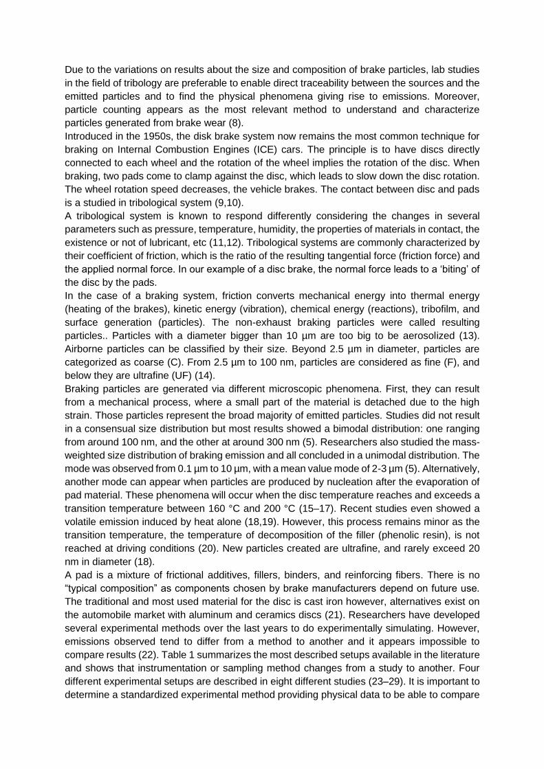
(cf. Figure 1). It only slides on one side of the disc.
Figure 1: Scheme of a pin-on-disc
Studies have shown the relevancy of pin-on-disc in braking particle investigation (25,44).
Affordable and easy to use, pin-on-disc seems to be a good option for braking studies.
1.4. On–road tests
On-road tests are also a method to simulate braking emission (28,44,46). On-road tests aim
to assess the braking emission on a driving vehicle. Hence, the friction materials and airflow
conditions are similar to driving conditions. This experiments investigates braking for the
brake emission assessment because of the difficulty involves in the collection of emitted
particles. So, these studies will remain rare due to its high level of contamination. External
parameters such as temperature, humidity, or wind are difficult to control. Those parameters
can cause significant tribological and airflow disturbances. WLTP cycle has been elaborated
to represent worldwide driving conditions. When on-board tests are not done on the track,
the equipped car has to obey traffic rules. But, the WLTP cycle is difficult to apply in real-life
conditions like urban traffic.
1.5. Cooling Temperature has a clear impact on on brake emission (3,16,30,40,42). Friction in braking
systems is a strong source of thermal energy. Therefore, discs are so designed to ensure their
viability.
While on-road tests are directly cooled by air, like in real-life conditions, pin-on-discs and
dynamometers need a cooling system. Brake discs are engineered to be good heat dissipaters.
They are thermally conductive and designed with holes and ventilation channels. However, the
system is closed and, air flow is still necessary to cool it. Flow rate leans on the cooling capacity
of the system. For the same geometry, higher flow rates induce a higher cooling rate, and so
lower temperatures are observed. In the WLTP cycle, braking events are paired to
corresponding temperatures (cf. part 1.1). An equivalent cooling system has not been defined
and, the researchers are using different cooling air flow for their experiments. Hagino et al. use
a flow rate of 30m3/h to ensure instrument accuracy (47). Whereas, Gramstat et al. performed
tests with a flow rate of 3450 m3/h. This discrepancy indeed could influence the emission rate,
but it also changes the whole air flow, by increasing the turbulence intensity (31,42,48).

2. Generated particles representativeness and confinement Over the last years, several authors (23,47,49,50) studied the sampling part of the
measurement. Yet no consensus on a proper reliable and, the repeatable protocol has been
reached. The repeatability of the sampling protocol lays mainly in the representativeness of
the particle flow. Emitted and measured particle distributions should be similar; if not, particle
losses have to be estimated to reduce them or, a correction can be applied to compensate for
the effects to trace the emitted distribution from the measured one. Finally, it is necessary to
consider the impact of the time transport of the sampling method on the representativeness.
2.1. Aerosol representativeness
Aerosol characterization instruments cannot analyze a large quantity of air and, only a small
fraction of generated particles are analyzed. In the field of braking measurement, the ELPI flow
rate corresponds to 10 L/min (0,6 m3/h) (cf. part 3). Compared to the actual cooling flow rate
of the chamber (average of 1.103m3/h, cf. part 1.5), this flow appears low. For
representativeness and repeatability matters, this sampling flow must be representative of the
whole emitted particles. To quantify the representativeness of the particles in the pipe, several
air samples are collected through different places.
Some laboratories assess the representativeness of their system (51). Those investigations
are only relatable to the specific air flow performances of the used dynamometer bench. All
the dynamometer chambers used for braking particle investigations differ in terms of flow rate,
geometry, or isokinetism. Representativeness can be achieved through different methods.
2.1.1. Characterization of diffuse emission
A sampling system aims at collecting a representative part of the aerosol as efficiently as
possible and then transports it through tubing or a sample line to an instrument to characterize
it (see fig 2). The global efficiency is expressed as the fraction of the aspirated aerosol through
the opening inlet concerning particle available in the source and cumulates with transport
efficiency through the sampling line. At that stage, two critical points are addressed
1. the inlet efficiency defined as the part of particles sampled and introduced in the inlet
concerning particle available in the source and
2. the transport efficiency which is the part of the particles introduced in the inlet and
reaching the instrument to the available particles at the opening inlet (52).
Figure 2 : Measurement of diffuse emission
In the field of aerosol physics, particle behavior is mainly driven by their size. Very small
particles will follow the streamlines and will be easily aspirated through the inlet plane with high
efficiency. However, larger particles like supermicronic ones are driven notably by inertia
forces and then weakly influenced by flow rate changes. Thus, most of the reasons that prevent
representative sampling deal with the aerosol particle size. In general, larger particles are more
actively influenced by mass forces such as gravitational and inertial forces, making a
representative sampling more difficult whereas, smaller particles like submicronic ones or
nanoparticles with higher diffusion coefficients are more easily lost to the walls of the sampling
system. Generally speaking, the 8 main factors that can influence the aerosol characterization
during the sampling are (52):
1. Aspiration efficiency and deposition in the opening inlet during sampling.
2. Deposition on the wall when the particles are transported through a sampling line.
3. Extremes (high or low) or variations in the ambient aerosol concentration.
4. Particle agglomeration during their passage through the sampling line.
5. Thermodynamically induced phenomena such as evaporation and /or condensation
6. Aerosolization of particles which were provisionally deposited on the walls
7. Local effects such as throttling by built-ups in the conduct
8. The effects of inhomogeneities of the particle concentrations in the conduct are due to
the result of lacking isokinetism.
Existence of wear with metallic materials, two other factors can be added:
1. charged particles can be generated by mechanical frictions and interact with the near
electric fields and on the inside of the inlet bring about a bias in sampling
2. chemical changes due to redox reactions caused by mechanical stress or compound
reactivity accentuated by size decrease and, it can transform the generated aerosol
during sampling time and transport.
All these factors are based on physical laws and, the main of them are detailed in the following
sections of this chapter. Nevertheless, In the field of particles generated by braking, the
difficulties are accentuated because of the severe conditions in temperatures, mechanical
stress and, inconstant concentration observed during their production. In that case, great
attention should be paid to the means of keeping the original aerosol during the sampling and
transport process to have a relevant characterization.
2.1.2. Isokinetism
Representative collection and reliable transport of a diffuse aerosol from a source to
characterization equipment is reported as a common difficulty and, achieving an accurate
description of the emitted aerosol are often described by literature as a challenge (52). An
aerosol sampling system consists of:
1. the particles are introduced in the opening intet of the measurement chain using a
suction system for extracting the aerosol sample from its ambient environment,
2. a sample conduct tube to convey the aerosol sample to the measuring instruments, to
a collection or a storage system, and, of course,
3. the instruments or samplers making the aerosol characterization possible.
Introduced as a concept of aerosol sampling in the 1950s, (53,54), isokinetic sampling allows
for sampling an aerosol without changing its properties, especially its size/mass distribution.

The flow containing particles shall not be biased by sampling air flow, i.e. setting the sampling
velocity to the level of the flow’s velocity. (Figure 3).
Figure 3 : Illustration of isokinetic sampling
Velocity differences can be a source of more or less fine or big particles in the sample flow,
which means a shift of the size/mass distribution. The disturbances can be a source of bias in
the distribution measurement. This bias can be understood via a dimensionless value: the
Stokes number. The Stokes number indicates the ability of a particle to follow fluid streamlines.
It can be calculated thanks to the following equation (55,56) :
𝑆𝑡𝑘 = 1
18
𝜌𝑝𝑑𝑝²𝑈
𝑙0µ𝑔
( 1 )
With Stk, the Stokes number, no unit,
𝜌𝑝, the volumetric mass of the particle, in kg.m-3,
𝑑𝑝, the aerodynamic diameter of the particle, in m,
𝑈, the fluid velocity, in m.s-1,
𝑙0, the characteristic dimension of the pipe (usually the diameter of the pipe), in m,
µ𝑔, the fluid dynamic viscosity, in kg.m-1.s-1.
The larger the Stokes number is, the more a particle is driven by its inertia, and the less the
particle tends to follow the fluid’s streamlines. For Stk << 1, particles follow streamlines;
meanwhile for Stk >> 1, the particles are less driven by the flow. Sampling with a velocity lower
than the flow velocity can lead to underrepresent small particles. Thus, a drift occurs during
the measurement. Dennis et al. (53) stated that “The magnitude of error as reported in the
literature depends upon the particle size and ranges from 10 to 20% for a 20% deviation from
the isokinetic flow.”.
To implement isokinetic sampling in a system, the inlet section must be calculated to respect
the equation (2):
∅𝑖𝑛𝑙𝑒𝑡 = ∅𝑙𝑜𝑐𝑎𝑙√𝑈𝑖𝑛𝑙𝑒𝑡
𝑈𝑙𝑜𝑐𝑎𝑙
( 2 )
With ∅𝑖𝑛𝑙𝑒𝑡, the diameter of the inlet section in m,
∅𝑙𝑜𝑐𝑎𝑙, the diameter of the duct where the air is sampled, in m,
𝑈𝑖𝑛𝑙𝑒𝑡, the sampling velocity, often set by the instrument, in m.s-1,
And 𝑈𝑙𝑜𝑐𝑎𝑙, the velocity of the fluid in the pipe, in m.s-1.
The inlet section must be designed to reach the appropriate sampling flow velocity.
Researchers normally used a classical inlet section with a fixed diameter. It implies that the
flow velocity if the sampling flow rate is constant and it cannot vary over time. In real-life
conditions, the air flow around the brake system varies over time, and adjusting air flow over
the experiment could be a new step forward into the representativeness of braking emission.
If such variable air flow is observed, the inlet section flow would have to vary as well.
2.2. Sampling efficiency
Particle losses during transport are an inevitable part of particle flow experiments, but they
have to be quantified and minimized. These losses depend on several parameters such as
transport duration, flow velocity, particle diameter, environment properties, transport road,
chemical properties of particles and tubes, etc (52). Braking events cause emissions of
particles with a wide range of diameters, and this range constitutes the main challenge of
particle losses control.
3. External and internal contamination
The adequate confinement of the set-up is evaluated by the ratio of signal to the background
noise. This ratio is a function of the presence of further external particle sources,
instrumentation uncertainties, emission levels, sampling, and transport efficiencies. In most
experimental setups includes an over-pressurized chamber, a HEPA 14 filter is chosen for its
high efficiency.
4. Losses
After their emission, particles need to be brought to the instrumentation. However, several
particle loss phenomena can reduce transport efficiency. Every element of the system has a
chamber, a sampling pipe connected to instrumentation induces a risk of loss. This chapter
presents the losses of particles in air flow. Estimating sampling loss impact is an important task
to characterize the originally emitted aerosol. Loss estimation has been obtained with oleic
acid monodisperse aerosol. Park et al. (57) reported that polydisperse aerosol highlights a
significantly higher wall deposition rate compared to a monodisperse solution.
2.2.1.1. Diffusion loss
Brownian motion of particles is a stochastic movement due to collisions of particles with fluid
molecules (52,58). The smaller the particles are, the more they are affected by collisions. The
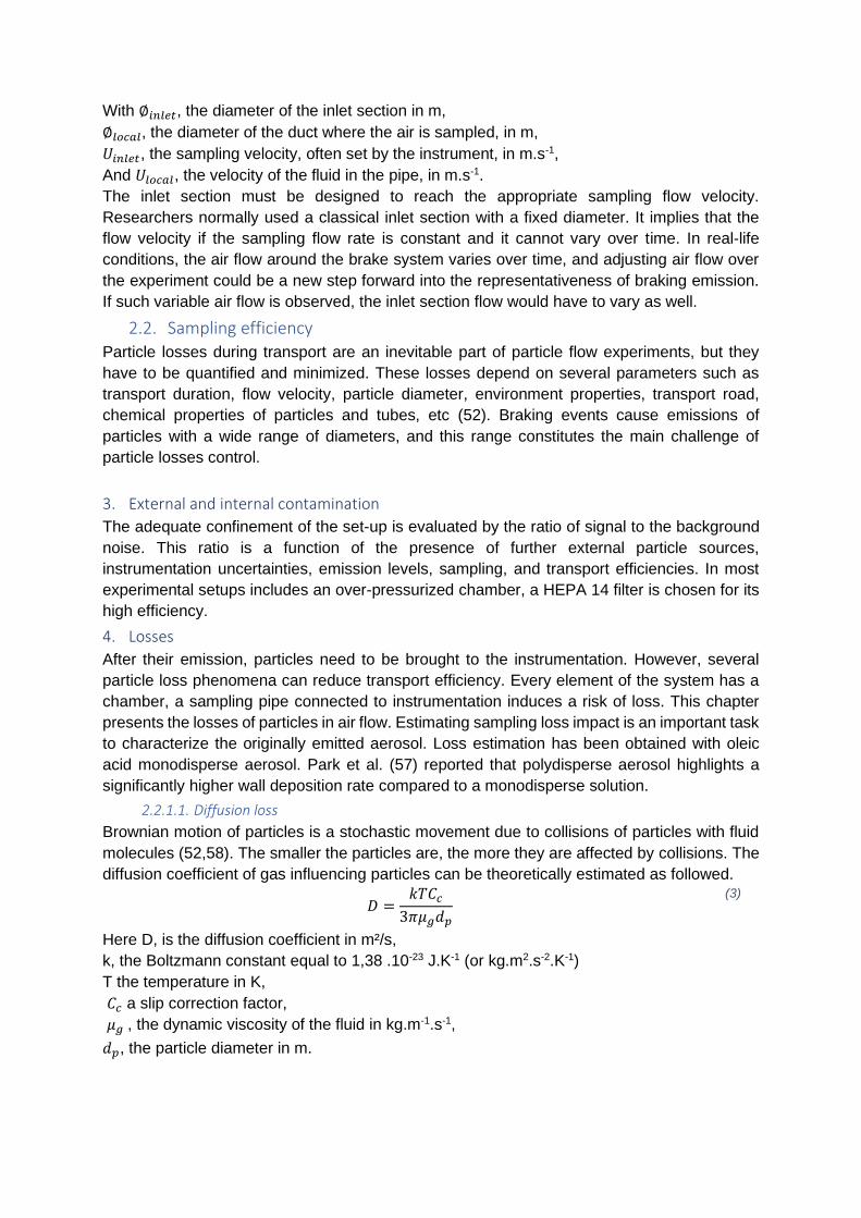
diffusion coefficient of gas influencing particles can be theoretically estimated as followed.
𝐷 =𝑘𝑇𝐶𝑐
3𝜋𝜇𝑔𝑑𝑝
(3)
Here D, is the diffusion coefficient in m²/s,
k, the Boltzmann constant equal to 1,38 .10-23 J.K-1 (or kg.m2.s-2.K-1)
T the temperature in K,
𝐶𝑐 a slip correction factor,
𝜇𝑔 , the dynamic viscosity of the fluid in kg.m-1.s-1,
𝑑𝑝, the particle diameter in m.

In brake emission investigations, air pressure and temperature can barely differ from standard
conditions. Thus, in equation (3) the slip correction factor 𝐶𝑐 and can be estimated with the
formula (4) (57):
𝐶𝑐 = 1 + 2𝜆
𝑑𝑝(1.246 + 0.418 exp (−
0.867𝑑𝑝
2𝜆)
(4)
Here, λ is the mean free path length of the gas molecules in m
Now the coefficient of diffusion D, and the Sherwood number Sh are defined. It is possible to
estimate transport efficiency ɳ𝑡𝑢𝑏𝑒,𝑑𝑖𝑓𝑓 regarding diffusion loss with the following formula:
ɳ𝑡𝑢𝑏𝑒,𝑑𝑖𝑓𝑓 = exp (−𝜋𝐷𝐿𝑆ℎ
𝑄)
(5)
Here Q, is the volumetric fluid flow in m3.s-1
L, the lenght of the duct in m
In most cases, those losses are theoretically highly negligible. The main reason is the high
flowrate equipment developed by research groups. It substantially decreases the diffusion time
of particles, which are less subject to encounter a wall in this period.
The Sherwood number is calculated as follow:
𝑆ℎ = 0,0118 𝑅𝑒7
8⁄ . (𝜇𝑔
𝜌𝐷)
13⁄
(6)
With Sh, the Sherwood number; and Re, the Reynolds number (cf. equation 9).
Sh is the mass transfer coefficient (59,60). Like many other fluid mechanic parameters, it is
possible to avoid complex computation thanks to an approximating formula (61).
2.2.1.2. Losses due to impaction and inertia forces
The first kind of loss is caused by bends in pipes. The transport to the instruments is usually
done via a pipe, which in case of spatial difficulties must be bent. The impact of bends on
transport efficiency is highly described in the literature (49,55,56,62–70). Agudelo et al. even
proposed different transporting design to minimize losses. Cheng and Wang’s (64) computing
method applies to laminar flow, whereas the method of Pui et al. (67) is relevant to turbulent
flow. Regarding bent pipes, Pui et al. declared that “the most important parameters are Stokes
number and the flow Reynolds number if particle motion is in the Stokesian regime (Rep ≤ 1)”
and proposed by to estimate the transport efficiency through a bent pipe as a function of Stokes
number:
ɳ𝑏𝑒𝑛𝑑 = 10−0,963.𝑆𝑡
(7)
With ɳ𝑏𝑒𝑛𝑑, the transport efficiency and St the Stokes number. Equation (7) is the most relevant
computing method for most of the researcher’s equipment. Computing with higher precision is
possible but, is time and cost consuming and consequently rarely performed.
A similar mechanism appears when the pipe section of the pipe decreases. The contraction of
the pipe implies a change in the direction of the external streamlines. It results in particle loss
in external streamlines. Like bent tubing, contraction tubing affects mostly particles with Stokes
number greater than 1. In 1996, Muyshom et al. proposed the empirically found relation (8) to
estimate transport efficiency through a tubing contraction ɳ𝑐𝑜𝑛𝑡 (71) :
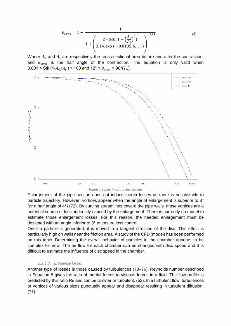
ɳ𝑐𝑜𝑛𝑡 = 1 − 1
1 + (2 ∗ 𝑆𝑡𝑘(1 − (
𝐴0𝐴𝑖
)2
)
3.14. exp ( −0.0185. 𝜃𝑐𝑜𝑛𝑡))
−1,24
(8)
Where 𝐴0 and 𝐴𝑖 are respectively the cross-sectional area before and after the contraction,
and 𝜃𝑐𝑜𝑛𝑡 is the half angle of the contraction. The equation is only valid when
0.001 ≤ Stk (1-𝐴0/𝐴𝑖 ) ≤ 100 and 12° ≤ 𝜃𝑐𝑜𝑛𝑡 ≤ 90°(71).
Figure 4. Losses in contraction fittings
Enlargement of the pipe section does not induce inertia losses as there is no obstacle to
particle trajectory. However, vortices appear when the angle of enlargement is superior to 8°
(or a half angle of 4°) (72). By curving streamlines toward the pipe walls, those vortices are a
potential source of loss, indirectly caused by the enlargement. There is currently no model to
estimate those enlargement losses. For this reason, the needed enlargement must be
designed with an angle inferior to 8° to ensure loss control.
Once a particle is generated, it is moved in a tangent direction of the disc. This effect is
particularly high on walls near the friction area. A study of the CFD (model) has been performed
on this topic. Determining the overall behavior of particles in the chamber appears to be
complex for now. The air flow for each chamber can be changed with disc speed and it is
difficult to estimate the influence of disc speed in the chamber.
2.2.1.3. Turbulence losses
Another type of losses is those caused by turbulences (73–76). Reynolds number described
in Equation 8 gives the ratio of inertial forces to viscous forces in a fluid. The flow profile is
predicted by this ratio Re and can be laminar or turbulent. (52). In a turbulent flow, turbulences
or vortices of various sizes punctually appear and disappear resulting in turbulent diffusion.
(77).

𝑅𝑒 = 𝜌𝑈𝐿
𝜇𝑔
(9 )
With Re, the Reynolds number
ρ, the volumetric mass in kg.m-3
U, the characteristic fluid speed in m.s-1
L, the characteristic linear dimension of the pipe (or else) in m
𝜇𝑔, the dynamic viscosity of the fluid in kg.m-1.s-1.
Under a critical value of the friction Reynolds number named Reτ , generally estimated between
2000-3000, no turbulence appears and the fluid is laminarly flowing (78). Meanwhile, if Re >
Reτ, the flow is turbulent. Equation 9 does not take into account local sources of variation of
the parameters such as irregularities on the pipe wall or particles in the air flow. As a result,
the limit between laminar and turbulent flow can change from one pipe to another. It is
expressed by the friction Reynolds number (Reτ). Turbulences are often generated close to
walls, where fluid shear stresses are higher (78).
When the inertia of particles is high enough, particles penetrate the sub-layer of air near the
wall and are hurting the wall (52). The transport efficiency ɳ𝑡𝑢𝑟𝑏 of particles passing through
a pipe is calculated by equation (10):
ɳ𝑡𝑢𝑟𝑏 = exp [−𝜋Ø𝐿𝑈𝑡
𝑄]
(10)
With Ø, the pipe section in m ;
L, the length of the pipe in m;
Ut, the turbulent inertial deposition velocity in m.s-1;
Q, the volumetric fluid flow in m3.s-1.
The turbulent inertial deposition velocity represents the velocity necessary to a particle to cross
the sub-layer and impact on the wall. Another expression of Ut is given by the equation (11):
𝑈𝑡 = 𝑈+ × √𝜏0
𝜌
(11)
Where:
𝑈+ is the dimensionless deposition velocity;
𝜏0 is the fluid shear stress in kg.m-1.s-² ;
ρ the volumic mass of the fluid in kg.m-3.
The formulas for the dimensionless deposition velocity is not properly defined. 𝑈+ has only
been approached by several approximated curve equations as a function of 𝜏+ (52,73,76). 𝜏+
is the dimensionless particle relaxation time, highly related to Stokes number :
𝜏+ = 𝑆𝑡𝑘 𝜏0. 𝑙0
𝜌. 𝑈²
(12)
All parameters are previously introduced in equation (1) and (11). 𝑈+ is described as a function
of 𝜏+. Literature concludes that the transport of particles is more efficient when 𝜏+ is close to
0.14.
2.2.1.4. Settling losses
Settling losses are a direct result of gravity on particles and are predominant for particles with
a diameter greater than 1 µm (see equation 5). Particles tend to settle over time. Sedimentation
velocity is proportional to the square of the particle diameter (Stokes Law) (52):
ß𝑠𝑒𝑡 =𝑈𝑠𝑒𝑡
ℎ. 𝜏𝑠𝑒𝑡
(13)
With ß𝑠𝑒𝑡 , the losses due to settling (no unit),
𝜏𝑠𝑒𝑡, the duration of dropping of a particle in chamber or pipe, in s,
𝑈𝑠𝑒𝑡, the terminal settling velocity in m.s-1,
h, the chamber or pipe height in m.
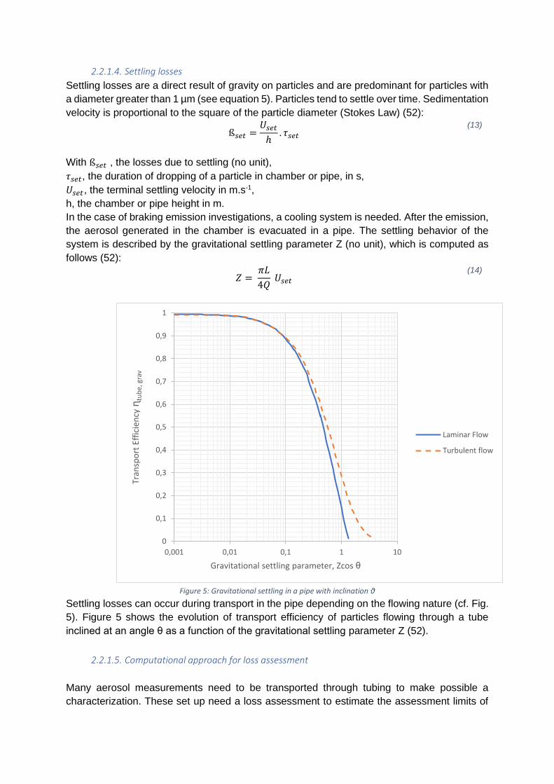
In the case of braking emission investigations, a cooling system is needed. After the emission,
the aerosol generated in the chamber is evacuated in a pipe. The settling behavior of the
system is described by the gravitational settling parameter Z (no unit), which is computed as
follows (52):
𝑍 = 𝜋𝐿
4𝑄 𝑈𝑠𝑒𝑡
(14)
Figure 5: Gravitational settling in a pipe with inclination θ
Settling losses can occur during transport in the pipe depending on the flowing nature (cf. Fig.
5). Figure 5 shows the evolution of transport efficiency of particles flowing through a tube
inclined at an angle θ as a function of the gravitational settling parameter Z (52).
2.2.1.5. Computational approach for loss assessment
Many aerosol measurements need to be transported through tubing to make possible a
characterization. These set up need a loss assessment to estimate the assessment limits of
0
0,1
0,2
0,3
0,4
0,5
0,6
0,7
0,8
0,9
1
0,001 0,01 0,1 1 10
Tran
spo
rt E
ffic
ien
cy ɳ
tub
e, g
rav
Gravitational settling parameter, Zcos θ
Laminar Flow
Turbulent flow

sizing, counting, and sampling. Von der Weiden, et all develop a software tool named Particle
Loss Calculator, (PLC) able to determine aerosol sampling efficiency and particle transport
losses due to passage through tubing (72)
The software takes into account different aspects of loss to give a relevant particle loss
assessment and includes the most important sampling and transport effects like a variation on
tubing, flow rate, bending. Other points are treated by software like non-isoaxial and non-
isokinetic aerosol sampling, aerosol diffusion and sedimentation which interest the braking
particle sampling (72). Thus, aerosol sizing obtained by equipment could be corrected by this
loss estimation and could lead to a more precise description of the original brake particles
emitted near the friction contact.
2.2.2. Chamber design
2.2.2.1. Response time
Response time is defined here as the elapsed time between the emission of particles and their
measurement. In a case of high response time, the last particles emitted from the first event
can be measured with the first particles emitted from the second event. This cross-
contamination can have different effects depending on the instrumentation and their own
sampling frequency. The paragraph here reminds the necessity to prefer low response time.
The notion of response time is a direct result of the residence time of particles in the chamber
(23). The difficulty to anticipate the air motion in the chamber causes trouble to estimate losses
(79). Some work was performed in controlled conditions (80–82) but, there is no theoretical
model that has been found yet. The residence time of particles in the chamber can be
estimated by the time of renewal of the chamber air (50) :
𝜏𝑐ℎ𝑎𝑚𝑏𝑒𝑟 = 𝑄𝑡𝑜𝑡𝑎𝑙
𝑉𝑐ℎ𝑎𝑚𝑏𝑒𝑟
(15)
With 𝜏𝑐ℎ𝑎𝑚𝑏𝑒𝑟, the complete renewal chamber air in min-1
𝑄𝑡𝑜𝑡𝑎𝑙, the total inlet or outlet flow in m3.min-1
𝑉𝑐ℎ𝑎𝑚𝑏𝑒𝑟, the volume of the chamber in m3
This estimation showcases two approaches to increase complete renewal chamber air:
On the one hand, it is possible to lower the chamber volume. In general, the literature shows
that the chamber size is under 0,817m3 (38) with an average value under 0,2 m3. However,
the main issue of a small chamber is the inevitable impaction inertia losses due to the motion
of particles directly on the wall after their emission from the brake system (cf. part 2.2.2.2.).
On the other hand, increasing the total flow of the experiment is also a solution. Researchers
design chambers with different flow values from 7.7 m3/h to 3450 m3/h, with an average value
of around 103 m3/h (16).
Response time can be changed in various ways that were all detailed in the previous part:
decreasing chamber size, increasing flow rate, and decreasing pipe section can lower the time
between emission and measurement. However, the time between emission and measurement
has not been defined yet; it is an open question. In real conditions, the average time where a
particle stays airborne is unknown and is impossible to define. Physical phenomena, such as
nucleation or aggregation (16,83) occur but, it is impossible to know their impact.

2.2.2.2. Electrostatic deposition and thermophoretic effect
Researchers chose two different materials: steel or acrylic glass to confine set-up. Steel is the
most used material (38,49, and few authors use acrylic glass (25). Steel is a conductive
material, which avoids electrical charges and limits the electrostatic deposition of charged
aerosol. Indeed, studies have shown the impact of using different materials on wall deposition
(56,68,84–87).
The thermophoretic deposition is another common loss of particles (88,89). If a wall is colder
than ambient air, thermophoretic deposition can be observed. The gradient of temperature in
a gas can lead to the migration of particles to the colder area. Those effects are difficult to
assess.
2.2.2.3. Geometry and layout of the chamber
The best place for the tribological contact, the orientation of disc, location of inlet, and outlet of
the chamber shall be defined to minimize particle losses.
The proximity of walls near disc and pads is a high source of loss. Hence except for one case
(51) where the chamber is large enough to assume that direct impaction is negligible, most of
the tribological contacts are placed in the center of the chamber (7,23).
In the case of the axial orientation of the disc, it is usually vertical, like real-life braking
conditions. At least one group works with a horizontal disc (90).
3. Number characterization of generated aerosols
3.1. Aerosol Particle Sizer (APS) In Aerosol Particle Sizers, the particle aerosol flows through a cell with a laser beam. Particle
in the cell diffuse light depending on their size and morphology (91). A photodetector converts
the light pulses into an electrical signal. The number concentration and the aerodynamic
diameter of the equivalent sphere can be determined with height and number of pulses based
on Mie’s theory (92). The particle’s refraction index must be known. Those instruments are
used to determine size distribution between 0,5 µm and 20 µm. This size range can be deemed
as irrelevant for isolated nano-particle investigations. An APS measurement added to an
SMPS measurement (see part 3.4.) can be used to assess aggregate and agglomerate
impacts.
3.2. Condensation nucleus counters (CNC) Condensation Nucleus Counters (CNC) or Condensation Particle Counters (CPC) are
standard devices used to determine particle number concentration in an aerosol. Particles
below 100 nm are unmeasurable by direct detection of laser counting. Particles are placed in
a saturated environment, with a high vapor pressure liquid, usually butanol, isopropanol, or
water. Vapors and particles are then cooled which, leads to condensation of vapors on the
particle surface. This condensation enlarges particles. The enlarged particles are now
detectable by the optical system placed after the condenser. This optical system is composed
of a laser and two photodetectors. One photodetector is used as a background reference when
no particle crosses the laser beam. The other photodetector catches the light diffused by
particles. Several models of CNC exist and, their size range varies from one to another. For
example, TSI CPC 3776 counts particles from 4 nm to 3 µm while TSI CNC 3007 only counts
from 10 nm to 1 µm.

3.3. Electrical Low Pressure Impactor (ELPI) ELPI selects solid particles by their inertia and then electrically detects them (93). Particles are
charged with a corona charger before being introduced to the cascade impactor. Particles are
then collected in a series of 13 impactors depending upon their size. Each floor is equipped
with an electrical counting system. ELPI classifies particles with diameters between 7 nm and
10 µm in 13 specific ranges. ELPI provides a simultaneous estimate at all channels, thus
aerosol sizing can be assessed with a short response time of between 1 and 20 seconds. ELPI
is not relevant for low concentration aerosols. The risk of bouncing of the particles can bias the
sizing. Using the most sensitive range, ELPI has a detection limit of 130 #/cm3 at 0.05 µm of
diameter, 5 #/cm3 at 0.5 µm and 0.4 #/cm3 at 5 µm (94).
3.4. Scanning Mobility Particle sizer Spectrometer (SMPS) SMPS is used to assess size distribution and number concentration of particles between 2,5
and 1 000 nm (95). A classifier, DMA (Differential Mobility Analyser), selects particles by their
size in a large number of channels. Aerosol firstly goes through an impactor that will retain the
biggest particles. It passes through a radioactive source (85Kr, 75 MBq intensity) or through
an X-ray source, called neutralizer, which charges particles with a high concentration of ions.
The aerosol passes then in a column where an adjustable electric field is applied between two
electrodes inducing a further motion of the previously charged object. This particle motion is
proportional to their size, making possible the size selection of the particles.
Only the particles with a known diameter and charge are extracted from the DMA as a
monodisperse aerosol.
The SMPS is the addition of a DMA and a CNC. The DMA is used to assess the size of particles
but, the CNC counts the extracted particles to obtain concentration. The SMPS needs to
browse size ranges from one after another with affecting time resolution. SMPS can determine
aerosol sizing in 20 seconds minimum.
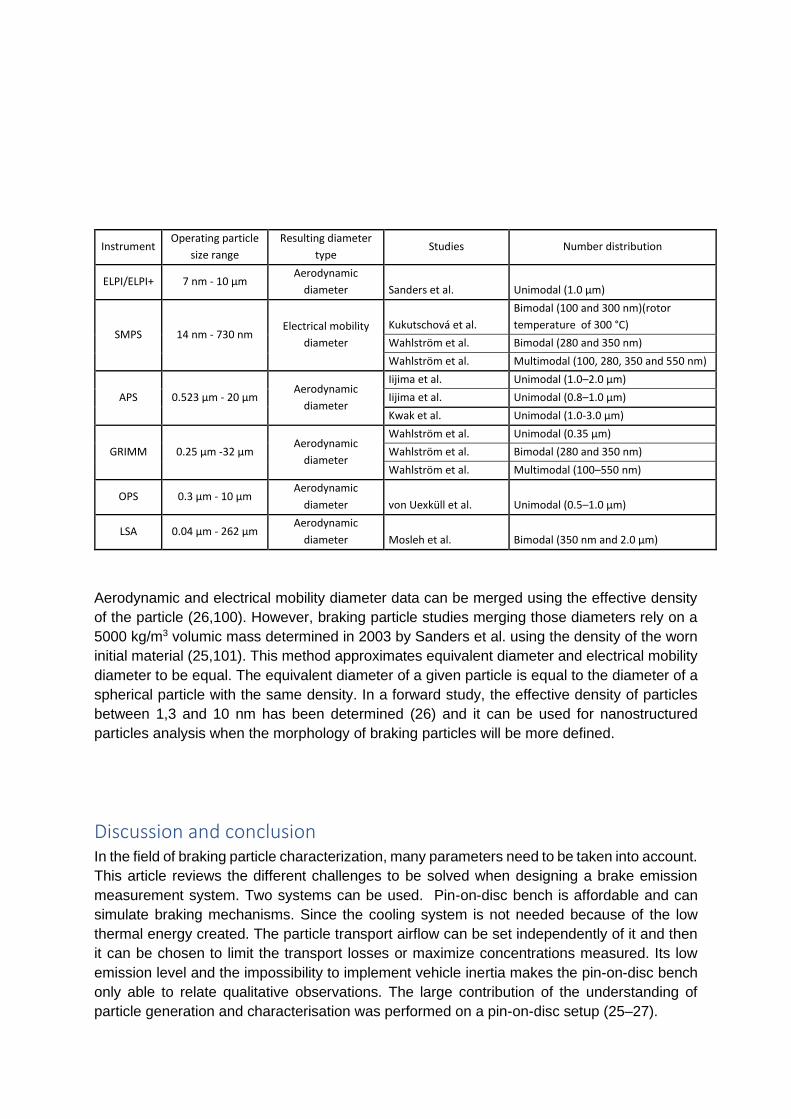
3.5. Instrumentation comparison As described in previous parts, instrumentation use different operating procedures that can
lead to different results (96–98). Even if instruments provide generally similar results in a
controlled sampling setting (96). Divergences can be observed at low number concentration
and the lower and upper working size ranges of the instruments (96). The type of particle
measured can also lead to the measurement of some error depending on instrumentation (96).
Price et al. showed, for instance, that FMPS identified bimodal distribution for TiO2 and fumed
silica, whereas the distribution generated was unimodal (96). Table 2 resumes instrumentation
used in braking particle domain, their working size, the type of particle diameter provided, the
related studies, and the modes identified. It has to be kept in mind that all studies can differ in
the experimental protocol but also in braking material used. Hence, number characterization
cannot be discussed here as other parameters are also varying. The Resulting diameter
type of Table 2 column is here to specify the outcoming diameters from instrumentation, which
are not directly comparable. The aerodynamic diameter of a particle is meant to describe
inertial properties in the gas. The aerodynamic diameter of a given particle is equal to the
diameter of a spherical particle with a density of 1 (99). Electrical mobility is used to classify
particles upon their ability to react to an electrical field. Algorithms are applied to determine
which diameter is equivalent to given electrical mobility (95).
Instrument Operating particle
size range
Resulting diameter
type Studies Number distribution
ELPI/ELPI+ 7 nm - 10 µm Aerodynamic
diameter Sanders et al. Unimodal (1.0 µm)
SMPS 14 nm - 730 nm Electrical mobility
diameter
Kukutschová et al.
Bimodal (100 and 300 nm)(rotor
temperature of 300 °C)
Wahlström et al. Bimodal (280 and 350 nm)
Wahlström et al. Multimodal (100, 280, 350 and 550 nm)
APS 0.523 µm - 20 µm Aerodynamic
diameter
Iijima et al. Unimodal (1.0–2.0 μm)
Iijima et al. Unimodal (0.8–1.0 μm)
Kwak et al. Unimodal (1.0-3.0 µm)
GRIMM 0.25 µm -32 µm Aerodynamic
diameter
Wahlström et al. Unimodal (0.35 µm)
Wahlström et al. Bimodal (280 and 350 nm)
Wahlström et al. Multimodal (100–550 nm)
OPS 0.3 µm - 10 µm Aerodynamic
diameter von Uexküll et al. Unimodal (0.5–1.0 μm)
LSA 0.04 µm - 262 µm Aerodynamic
diameter Mosleh et al. Bimodal (350 nm and 2.0 μm)
Aerodynamic and electrical mobility diameter data can be merged using the effective density
of the particle (26,100). However, braking particle studies merging those diameters rely on a
5000 kg/m3 volumic mass determined in 2003 by Sanders et al. using the density of the worn
initial material (25,101). This method approximates equivalent diameter and electrical mobility
diameter to be equal. The equivalent diameter of a given particle is equal to the diameter of a
spherical particle with the same density. In a forward study, the effective density of particles
between 1,3 and 10 nm has been determined (26) and it can be used for nanostructured
particles analysis when the morphology of braking particles will be more defined.
Discussion and conclusion In the field of braking particle characterization, many parameters need to be taken into account.
This article reviews the different challenges to be solved when designing a brake emission
measurement system. Two systems can be used. Pin-on-disc bench is affordable and can
simulate braking mechanisms. Since the cooling system is not needed because of the low
thermal energy created. The particle transport airflow can be set independently of it and then
it can be chosen to limit the transport losses or maximize concentrations measured. Its low
emission level and the impossibility to implement vehicle inertia makes the pin-on-disc bench
only able to relate qualitative observations. The large contribution of the understanding of
particle generation and characterisation was performed on a pin-on-disc setup (25–27).

Inertia dynamometer bench studies involve considerable investment. However, this system
might become fundamental to future standardization as it could provide measurements in real-
life conditions. The high thermal energy dissipated by the friction forces to use an airflow to
keep the friction material cool. Inertia dynamometer bench can simulate real driving conditions.
The representativeness of friction material temperatures can be achieved with respect to
WLTP cycle (20). It has to be noted that WLTP disc temperature was determined on road, with
a specific vehicle (inertia) and a specific braking system. The determined temperature cycle
represents driving cooling conditions. The same specific parameters (inertia and braking
system) can be used to fit the disc temperatures of the cooling system in the dynamometer
bench. The bench can be used to investigate the other braking systems/materials using those
same cooling conditions, which represent real cooling conditions.
Today, the representativeness of braking particle characterization is under question.
Estimation losses can be computed with techniques exposed above. An important point to
know about the losses concerns in the sampling pipe, where a high flow rate can be preferred
to improve aerosol transport and reduce diffusion and settling losses. It should be pointed out
that a too high velocity can lead to turbulence losses and a too-high flow rate leads to low
particle concentrations. If the setup requires bending, a lower flow velocity can be set, either
by increasing the inlet section or by decreasing the flowrate.
In a broader context, understanding and measurement of braking emission still lack several
knoweldge gaps:
- Understanding of generation mechanisms has still to be developed. The origin of
particles and their behavior in the contact is still an open question.
- Simulation of emission mechanisms is out of range for the moment because of the
large surfaces to take into account and the complexity of pad compositions. Braking
emission cannot be estimated by computing.
- Losses in the chamber are today difficult to estimate, and the best way to avoid these
is to shorten the residence time of particles in the chamber.
- Instrumentation is used to assess the emissions changes from a study to another and
can influence the data. A stabilized measurement protocol based on a consensus on
equipment could increase the comparability of the results. A better characterization of
particles would help to describe the link between the different kinds of diameters used
by instrumentation.
Acknowledgment
The authors gratefully acknowledge our respective institutions for making this
transdisciplinary project possible. Also, we acknowledge the financial support of the ANRT
grant number in this project. The French Ministry for Ecology funding is gratefully
acknowledged.
Declaration of conflicting interests The author(s) declared no potential conflicts of interest with respect to the research, authorship, and/or publication of this article.
Funding The author(s) disclosed receipt of the following financial support for the research, authorship, and/or publication of this article: This work is supported by the ANRT for the grant number and the French Ministry for Ecology for the funding.
Bibliography
1. Yan F, Winijkul E, Jung S, et al. Global emission projections of particulate matter (PM): I.
Exhaust emissions from on-road vehicles. Atmos Environ 2011; 45(28): 4830–4844.
2. Hulskotte JHJ, Roskam GD and van der Gon HD. Elemental composition of current
automotive braking materials and derived air emission factors. Atmos Environ 2014; 99: 436–
445.
3. Grigoratos T and Martini G. Non-exhaust traffic related emissions. Brake and tyre wear
PM. [Internet], https://core.ac.uk/download/pdf/38628016.pdf (2014, accessed25 May 2020).
4. Guerreiro C, Hora’ lek J, de Leeuw F, et al. Air quality in Europe: 2015 report [Internet].
Luxembourg: publications Office. http://bookshop.europa.eu/uri?target=EUB:NOTICE:
THAL15005:EN:HTML (2015, 4 November 2019).
5. Grigoratos T and Martini G. Brake wear particle emissions: a review. Environ Sci Pollut
Res 2015; 22(4):2491–2504.
6. Thorpe A and Harrison RM. Sources and properties of non-exhaust particulate matter from
road traffic: a review. Sci Total Environ 2008; 400(1): 270–282.
7. Hagino H, Oyama M and Sasaki S. Laboratory testing of airborne brake wear particle
emissions using a dynamometer system under urban city driving cycles. Atmos Environ
2016; 131: 269–278.
8. EEA E. Air quality in Europe - 2015 report. Report no. 5/ 2015, 2015. Copenhagen:
European Environment Agency.
9. Eriksson M, Bergman F and Jacobson S. On the nature of tribological contact in
automotive brakes. Wear 2002; 252(1): 26–36.
10. Eriksson M and Jacobson S. Tribological surfaces of organic brake pads. Tribol Int 2000;
33(12): 817–827.
11. Halling J. Principles of tribology.Macmillan International Higher Education, 1978, p.414.
12. Bhushan B. Introduction to tribology. New York, NY: John Wiley & Sons, 2013, p.672.
13. Williams MMR and Loyalka SK. Aerosol science: theory and practice,
http://inis.iaea.org/Search/search.aspx?orig_q=RN:23024824 (1991, accessed 9 October
2019).
14. Liu L, Urch B, Poon R, et al. Effects of ambient coarse, fine, and ultrafine particles and
their biological constituents on systemic biomarkers: a controlled human exposure study.
Environ Health Perspect 2015; 123(6): 534–540.
15. Alemani M, Nosko O, Metinoz I, et al. A study on emission of airborne wear particles from
car brake friction Pairs. SAE Int J Mater Manf 2015; 9(1): 147–157.
16. Nosko O, Vanhanen J and Olofsson U. Emission of 1.3– 10 nm airborne particles from
brake materials. Aerosol Sci Technol 2017; 51(1): 91–96.
17. Wahlstro‥m J, Olander L and Olofsson U. A pin-on-disc study focusing on how different
load levels affect the concentration and size distribution of airborne wear particles from the
disc brake materials. Tribol Lett 2012; 46(2): 195–204.
18. Ma J, Olofsson U, Lyu Y, et al. A comparison of airborne particles generated from disk
brake contacts:

induction versus frictional heating. Tribol Lett 2020; 68(1): 38.
19. Perricone G, Mata’ jka V, Alemani M, et al. A test stand study on the volatile emissions of
a passenger car brake assembly. Atmosphere 2019; 10(5): 263.
20. Mathissen M, Grochowicz J, Schmidt C, et al. A novel real-world braking cycle for
studying brake wear particle emissions. Wear 2018; 414–415: 219–226.
21. Maleque MA, Dyuti S and Rahman MM. Material selection method in design of
automotive brake disc. In: Proceedings of the world congress on engineering, London, UK,
30 June–2 July 2010, vol. III, p.5.Philippe et al. 13
22. Chan D and Stachowiak GW. Review of automotive brake friction materials. Proc
IMechE, Part D: J Automobile Engineering 2004; 218(9): 953–966.
23. Perricone G, Wahlstro‥m J and Olofsson U. Towards a test stand for standardized
measurements of the brake emissions. Proc IMechE, Part D: J Automobile Engineering
2016; 230(11): 1521–1528.
24. Hagino H, Oyama M and Sasaki S. Airborne brake wear particle emission due to braking
and accelerating. Wear 2015; 334–335: 44–48.
25. Wahlstro‥m J, So‥ derberg A, Olander L, et al. A pin-on disc simulation of airborne
wear particles from disc brakes. Wear 2010; 268(5–6): 763–769. 26. Nosko O and Olofsson
U. Effective density of airborne wear particles from car brake materials. J Aerosol Sci 2017;
107: 94–106.
27. Alemani M, Wahlstro‥m J and Olofsson U. On the influence of car brake system
parameters on particulate matter emissions. Wear 2018; 396–397: 67–74.
28. Wahlström J and Olofsson U. A field study of airborne particle emissions from automotive
disc brakes. Proc IMechE, Part D: J Automobile Engineering 2015; 229(6): 747–757.
29. Kukutschova’ J, Moravec P, Toma’ sˇek V, et al. On airborne nano/micro-sized wear
particles released from lowmetallic automotive brakes. Environ Pollut 2011; 159(4): 998–
1006.
30. Mathissen M, Grigoratos T, Lahde T, et al. Brake wear particle emissions of a passenger
car measured on a chassis dynamometer. Atmosphere 2019; 10(9): 556.
31. Nosko O, Alemani M and Olofsson U. Temperature effect on emission of airborne wear
particles from car brakes. In: Proceedings of Europe’s braking conference and exhibition,
Dresden, Germany, 2015, p.18.
32. Perricone G, Mateˇjka V, Alemani M, et al. A concept for reducing PM 10 emissions for
car brakes by 50%. Wear 2018; 396–397: 135–145.
33. Nosko O, Alemani M and Olofsson U. Characterisation of airborne particles emitted from
car brake materials. In: 6th World tribology congress, Beijing, China, 17–22 September 2017,
p.5.
34. Ciudin R, Verma PC, Gialanella S, et al. Wear debris materials from brake systems:
environmental and health issues. WIT Trans Ecol Environ 2014; 191: 1423–1434.
35. Alemani M, Perricone G, Olofsson U, et al. A proposed dyno bench test cycle to study
particle emissions from disk brakes. In: Conference paper from Eurobrake 2014, Lille,
France, 13–15 May 2014. London: FISITA.
36. Timte M. A comparison of lining output generated using AK master and FMVSS 105
simulation dynamometer procedures [Internet], https://www.sae.org/publications/ technical-
papers/content/2000-01-2777/ (2000, accessed 25 août 2020).
37. Gramstat S, Cserhati A, Schroeder M, et al. Brake particle emission measurements -
testing method and results. SAE Int J Engines 2017; 10(4): 1841–1846.
38. Perricone G, Alemani M, Metino‥ z I, et al. Towards the ranking of airborne particle
emissions from car brakes –a system approach. Proc IMechE, Part D: J Automobile
Engineering 2017; 231(6): 781–797.
39. Demuynck J, Bosteels D, De Paepe M, et al. Recommendations for the new WLTP cycle
based on an analysis of vehicle emission measurements on NEDC and CADC. Energy
Policy 2012; 49: 234–242.
40. Kukutschova’ J, Roubı’cˇek V, Malachova’ K, et al. Wear mechanism in automotive brake
materials, wear debris and its potential environmental impact. Wear 2009; 267(5–8): 807–
817.
41. Iijima A, Sato K, Yano K, et al. Particle size and composition distribution analysis of
automotive brake abrasion dusts for the evaluation of antimony sources of airborne
particulate matter. Atmos Environ 2007; 41(23): 4908–4919.
42. Shin J, Yim I, Kwon S-B, et al. Evaluation of temperature effects on brake wear particles
using clustered heatmaps. Environ Eng Res 2019; 24(4): 680–689.
43. O‥ sterle W, Bresch H, Do‥ rfel I, et al. Surface film formation and dust generation
during brake performance tests.
New York, NY: The Institution of Mechanical Engineers, 2009.
44. Alemani M, Wahlstro‥m J, Mateˇjka V, et al. Scaling effects of measuring disc brake
airborne particulate matter emissions – a comparison of a pin-on-disc tribometer and an
inertia dynamometer bench under dragging conditions. Proc IMechE, Part H: J Engineering
Tribology 2018; 232(12): 1538–1547.
45. Kwak J, Kim H, Lee J, et al. Characterization of nonexhaust coarse and fine particles
from on-road driving
and laboratory measurements. Sci Total Environ 2013; 458–460: 273–282.
46. Farwick zum Hagen FH, Mathissen M, Grabiec T, et al. On-road vehicle measurements
of brake wear particle emissions. Atmos Environ 15 2019; 217: 116943.
47. Hagino H. Feasible methodology for brake wear particles measurement and
characterization. In: 45th PMP meeting, Joint Research Centre, Ispra, Italy, 7–8 November
2017, p.19.
48. Shabanian SR, Rahimi M, Shahhosseini M, et al. CFD and experimental studies on heat
transfer enhancement in an air cooler equipped with different tube inserts. Int Commun Heat
Mass Transfer 2011; 38(3): 383–390.
49. Agudelo C. PMP-45-15 LINK Design considerations for brake emission measurements.
2017.
50. Brembo S.p.A. REBRAKE: a brake test stand for particles measurement and collection.
2016.
51. Ansaloni S, Sin A and Moiso M. PMP-48-19 ITT presentation. 7–8 November 2018,
Ispra, Italy.
52. Kulkarni P, Baron PA and Willeke K. Aerosol measurement: principles, techniques, and
applications. Hoboken, NJ: John Wiley & Sons, 2011, p.904.
53. Dennis R, Samples WR, Anderson DM, et al. Isokinetic sampling probes. Ind Eng Chem
1957; 49(2): 294–302.
54. Wilcox JD. Isokinetic flow and sampling. J Air Pollut Control Assoc 1956; 5(4): 226–245.
55. Breuer M, Baytekin HT and Matida EA. Prediction of aerosol deposition in 90_ bends
using LES and an efficient Lagrangian tracking method. J Aerosol Sci 2006; 37(11): 1407–
1428.
56. Sun K and Lu L. Particle flow behavior of distribution and deposition throughout 90_
bends: analysis of influencing factors. J Aerosol Sci 2013; 65: 26–41.
57. Park SH, Kim HO, Han YT, et al. Wall loss rate of polydispersed aerosols. Aerosol Sci
Technol 2001; 35(3):
710–717.
58. Kim DS, Park SH, Song YM, et al. Brownian coagulation of polydisperse aerosols in the
transition regime. J Aerosol Sci 2003; 34(7): 859–868. 14 Proc IMechE Part D: J Automobile
Engineering 00(0)
59. Sherwood T and Wei J. Interfacial phenomena in liquid extraction. Ind Eng Chem 1957;
49(6): 1030–1034.
60. Sulaiman M, Climent E, Hammouti A, et al. Mass transfer towards a reactive particle in a
fluid flow: numerical simulations and modeling. Chem Eng Sci 2019; 199: 496–507.
61. Delattre P and Friedlander SK. Aerosol coagulation and diffusion in a turbulent jet. Ind
Eng Chem Fund 1978; 17(3): 189–194.
62. Berrouk AS and Laurence D. Stochastic modelling of aerosol deposition for LES of 90_
bend turbulent flow. Int J Heat Fluid Flow 2008; 29(4): 1010–1028.
63. Bluestein AM, Venters R, Bohl D, et al. Turbulent flow through a ducted elbow and
plugged tee geometry: an experimental and numerical study. J Fluids Eng 2019; 141(8):
081101–081101-14.
64. Cheng YS and Wang CS. Motion of particles in bends of circular pipes. Atmos Environ
1981; 15(3): 301–306.
65. Cong XC, Yang GS, Qu JH, et al. A model for evaluating the particle penetration
efficiency in a ninety-degree bend with a circular-cross section in laminar and turbulent flow
regions. Powder Technol 2017; 305: 771–781.
66. Crane RI and Evans RI. Inertial deposition of particles in a bent pipe. J Aerosol Sci 1977;
8: 161–170.
67. Pui DYH, Romay-Novas F and Liu BYH. Experimental study of particle deposition in
bends of circular cross section. Aerosol Sci Technol 1987; 7(3): 301–315.
68. Sun K, Lu L and Jiang H. A numerical study of bendinduced particle deposition in and
behind duct bends. Build Environ 2012; 52: 77–87.
69. Tsai C-J and Pui DYH. Numerical study of particle deposition in bends of a circular cross-
section-laminar
flow regime. Aerosol Sci Technol 1990; 12(4): 813–831.
70. Zhang P, Roberts RM and Be’nard A. Computational guidelines and an empirical model
for particle deposition in curved pipes using an Eulerian-Lagrangian approach. J Aerosol Sci
2012; 53: 1–20.
71. Muyshondt A, McFarland AR and Anand NK. Deposition of aerosol particles in
contraction fittings. Aerosol Sci Technol 1996; 24(3): 205–216.
72. von der Weiden S-L, Drewnick F and Borrmann S. Particle loss calculator – a new
software tool for the assessment of the performance of aerosol inlet systems. Atmos Meas
Tech 2009; 2(2): 479–494.
73. Chen Q and Ahmadi G. Deposition of particles in a turbulent pipe flow. J Aerosol Sci
1997; 28(5): 789–796.
74. Pozorski J. Models of turbulent flows and particle dynamics. In: Minier J-P and Pozorski J
(eds) Particles in
wall-bounded turbulent flows: deposition, re-suspension and agglomeration [Internet]. Cham:
Springer International
Publishing, 2017, pp.97–150.
75. Reynolds AM. A Lagrangian stochastic model for heavy particle deposition. J Colloid
Interface Sci 1999; 15(1): 85–91.
76. Wood NB. A simple method for the calculation of turbulent deposition to smooth and
rough surfaces. J Aerosol Sci 1981; 12(3): 275–290.
77. Bandyopadhyay PR and Balasubramanian R. Vortex Reynolds number in turbulent
boundary layers. Theor Comput Fluid Dyn 1995; 7(2): 101–117.
78. HudmanMand Hugh MB. Large eddy simulation of turbulent pipe flow. In: Second
international conference on CFD in the minerals and process industries, Melbourne, VIC,
Australia, December 1999, pp.369–374. Melbourne: CSIRO Australia.
79. Liu X, Zhang Y, Wu Q, et al. Study on the key structure parameters of a gravity settling
chamber based on a flow field simulation. Eng Appl Comput Fluid Mech 2019; 13(1): 377–
395.
80. Hussein T, Hrusˇka A, Doha’nyosova’ P, et al. Deposition rates on smooth surfaces and
coagulation of aerosol particles inside a test chamber. Atmos Environ 2009; 43(4): 905–914.
81. Hussein T, Kubincova’ L, Dzˇumbova’ L, et al. Deposition of aerosol particles on rough
surfaces inside a test chamber. Build Environ 2009; 44(10): 2056–2063.
82. Zhao B and Wu J. Particle deposition in indoor environments: analysis of influencing
factors. J Hazard Mater 2007; 147(1): 439–448.
83. Van Leussen W. Aggregation of particles, settling velocity of mud flocs a review. In:
Dronkers J and van Leussen W (eds) Physical processes in estuaries. Berlin, Heidelberg:
Springer, 1988, pp.347–403.
84. Keshani S, Daud WRW, Nourouzi MM, et al. Spray drying: an overview on wall
deposition, process and modeling. J Food Eng 2015; 146: 152–162.
85. Lai ACK. Investigation of electrostatic forces on particle deposition in a test chamber.
Indoor Built Environ 2006; 15(2): 179–186.
86. Stelling C, Mark A, Papastavrou G, et al. Showing particles their place: deterministic
colloid immobilization by gold nanomeshes. Nanoscale 2016; 8(30): 14556–14564.
87. Yu K-P, Lee W-MG, Peng C-J, et al. Effects of roughness, dielectric constant and
electrical resistivity of wall on deposition of submicron particles driven by ionic air purifier. J
Environ Chem Eng 2017; 5(4): 3108–3114.
88. Pratsinis SE and Kim K-S. Particle coagulation, diffusion and thermophoresis in laminar
tube flows. J Aerosol Sci 1989; 20(1): 101–111.
89. Walsh JK,Weimer AW and Hrenya CM. Thermophoretic deposition of aerosol particles in
laminar tube flow with mixed convection. J Aerosol Sci 2006; 37(6): 715–734.
90. Wahlstro‥m J, Lyu Y, Matjeka V, et al. A pin-on-disc tribometer study of disc brake
contact pairs with respect to wear and airborne particle emissions. Wear 2017; 384– 385:
124–130.
91. Wilson JC and Liu BYH. Aerodynamic particle size measurement by laser-Doppler
velocimetry. J Aerosol Sci 1980; 11(2): 139–150.
92. Hergert W and Wriedt T. The Mie theory: basics and applications. Berlin, Heidelberg:
Springer, 2012, p.268.
93. Keskinen J, Pietarinen K and Lehtima‥ kiM. Electrical low pressure impactor. J Aerosol
Sci 1992; 23(4): 353–360.
94. Marjama‥ ki M, Keskinen J, Chen D-R, et al. Performance evaluation of the electrical
low-pressure impactor (ELPI). J Aerosol Sci 2000; 31(2): 249–261.
95. Wang SC and Flagan RC. Scanning electrical mobility spectrometer. Aerosol Sci Technol
1990; 13(2): 230–240.
96. Price HD, Stahlmecke B, Arthur R, et al. Comparison of instruments for particle number
size distribution measurements in air quality monitoring. J Aerosol Sci 2014; 76: 48–55.
97. Peters TM, Ott D and O’Shaughnessy PT. Comparison of the Grimm 1.108 and 1.109
portable aerosol spectrometer to the TSI 3321 aerodynamic particle sizer for dry particles.
Ann Occup Hyg 2006; 50(8): 843–850. Philippe et al. 15
98. Tuch TH, Mirme A, Tamm E, et al. Comparison of two particle-size spectrometers for
ambient aerosol measurements. Atmos Environ 2000; 34(1): 139–149.
99. Sto‥ ber W. A note on the aerodynamic diameter and the mobility of non-spherical
aerosol particles. J Aerosol Sci 1971; 2(4): 453–456.
100. Thomas D, Charvet A, Bardin-Monnier N, et al. Aerosol filtration. Oxford: Elsevier, ISTE
Press, 2016, p.228.
101. Sanders PG, Xu N, Dalka TM, et al. Airborne brake wear debris: size distributions,
composition, and a comparison of dynamometer and vehicle tests. Environ Sci Technol
2003; 37(18): 4060–4069.