Embed Size (px)
Citation preview

8th International Purdue Symposium on Statistics June 21, 2012'
&
$
%
Reproducibility of Science:P-values and Multiplicity
Jim Berger
Duke University
8th International Purdue Symposium on StatisticsJune 21, 2012
1

8th International Purdue Symposium on Statistics June 21, 2012'
&
$
%
Outline
• Evidence of an increasing lack of reproducibility of science
• Some reasons for the lack of reproducibility
– Publication bias
– Experimental biases, including programming errors
– The very considerable rewards for ‘positive’ results
– Statistical biases
– Egregiously bad statistics
– The incorrect way in which p-values are used
– Failure to adjust for multiplicities
∗ Multiple testing
∗ Multiple looks at the data
∗ Multiple statistical analyses
• How Bayesian analysis can help
2

8th International Purdue Symposium on Statistics June 21, 2012'
&
$
%
I. Evidence for a Lack of Reproducibility
• “The reliability of results from observational studies has been called
into question many times in the recent past, with several analyses
showing that well over half of the reported findings are subsequently
refuted.” JNCI, 2007
• The NIH funded randomized clinical trials to follow up exciting results
from 20 observational studies. Only 1 replicated.
• Bayer Healthcare reviewed 67 in-house attempts at replicating the
findings in published research.
– Less than 1/4 were viewed as having been essentially replicated.
– Over 2/3 had major inconsistencies leading to project termination.
• John P. A. Ioannidis, JAMA-2005, 218-28: Five of 6 highly cited
nonrandomized studies were contradicted or had found stronger effects
than were established by later studies.
3

8th International Purdue Symposium on Statistics June 21, 2012'
&
$
%
Even the best studies often fail to replicate.
• Ioannidis looked at the 49 most famous medical publications from
1990-2003 resulting from randomized trials; 45 claimed successful
intervention.
– 7 (16%) were contradicted by subsequent studies
– 7 others (16%) had found effects that were stronger than those of
subsequent studies
– 20 (44%) were replicated
– 11 (24%) remained largely unchallenged.
• Phase II drug trials success rates are falling (28% 5 years ago, 18%
now) (Arrowsmith (2011) Nature Reviews Drug Discovery 10)
• 50% phase III drug trial failure rates are now being reported, versus a
20% failure rate 10 years ago (Arrowsmith (2011) Nature Reviews Drug
Discovery 10); 70% phase III cancer drug failure rate
• Reports that 30% of phase III drug trial successes fail to replicate
4

8th International Purdue Symposium on Statistics June 21, 2012'
&
$
%
II. Some Reasons for a Lack of Reproducibility
1. Publication bias:
• Negative (and especially small negative) studies are often never
reported or, if they are, can have publication delays of up to 3 years.
Figure 1: From Fanelli, D. Scientometrics 90, 891–904 (2011).
5

8th International Purdue Symposium on Statistics June 21, 2012'
&
$
%
• Ioannides: Looked at a meta-analysis of a widely studied head and
neck cancer:
– the meta-analysis reported on 80 published studies;
– they found 13 additional published studies not in the meta-analysis;
– they found 10 non-published studies, but were able to get the data;
– they found another 38 studies where data could not be obtained;
– who knows how many other studies were done leaving no record.
The original 80 provided significance at 0.05 in the meta-analysis; the
80+13 were barely significant; the 80+13+10 did not yield significance.
• Effect sizes for observational studies with small sample sizes tend to be
much larger than effect sizes for studies with large sample sizes.
6

8th International Purdue Symposium on Statistics June 21, 2012'
&
$
%
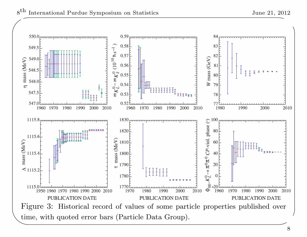
2. Experimental biases:
Figure 2: Historical record of values of some particle properties published over
time, with quoted error bars (Particle Data Group).
7
8th International Purdue Symposium on Statistics June 21, 2012'
&
$
%Figure 3: Historical record of values of some particle properties published over
time, with quoted error bars (Particle Data Group).
8

8th International Purdue Symposium on Statistics June 21, 2012'
&
$
%
3. The very considerable rewards for ‘positive’ results
• Money and fame
– “There is nothing wrong with cancer research that a little less money
wouldn’t cure.” (Nathan Mantel, NCI)
• Promotion and tenure
• Journals want high impact factors
• ...
• And, except perhaps for physics, there seems to be little to no
professional penalty for having a positive finding later refuted.
– What is the situation in this regard with statistics?
9

8th International Purdue Symposium on Statistics June 21, 2012'
&
$
%
4. Statistical biases
• Confounding, especially in observational studies
– Worse with large sample sizes
• Programming errors
“To err is human, but to really foul things up requires a computer.”
Farmers’ Almanac (1978)
• ...
10

8th International Purdue Symposium on Statistics June 21, 2012'
&
$
%
5. Use of egregiously bad statistics
5.1. Using statistics ‘as a language’:
Sander Nieuwenhuis, Birte U Forstmann Eric-Jan Wagenmakers, Nature
Neuroscience 14, 1105–1107 (2011).
• Reviewed 513 neuroscience articles in five top-ranking journals.
• Found 157 comparing ‘Treatment A’ and ‘Treatment B.’
– 78 correctly looked at the mean difference of effects for significance.
– 79 had at least one instance of incorrectly concluding that there was
a significant difference between the treatments if one was ‘significant
at the 0.05 level against a control’ and the other was not
(for instance, if zA = 1.97 and zB = 1.95 ).
5.2. Purposely ignoring statistical principles:
• The tradition in epidemiology is to ignore multiple testing.
• The tradition in psychology is to ignore optional stopping.
“You cannot ask us to take sides against arithmetic.” Winston Churchill
11

8th International Purdue Symposium on Statistics June 21, 2012'
&
$
%
6. The incorrect way in which p-values are used:
“To p, or not to p, that is the question?”
• Few non-statisticians understand p-values, most erroneously thinking
they are some type of error probability (Bayesian or frequentist).
– A survey 30 years ago:
∗ “What would you conclude if a properly conducted, randomized
clinical trial of a treatment was reported to have resulted in a
beneficial response (p < 0.05)?
1. Having obtained the observed response, the chances are less than 5%
that the therapy is not effective.
2. The chances are less than 5% of not having obtained the observed
response if the therapy is effective.
3. The chances are less than 5% of having obtained the observed
response if the therapy is not effective.
4. None of the above
∗ We asked this question of 24 physicians ... Half ... answered
incorrectly, and all had difficulty distinguishing the subtle differences...
∗ The correct answer to our test question, then, is 3.”
12

8th International Purdue Symposium on Statistics June 21, 2012'
&
$
%
“This isn’t right. This isn’t even wrong.” –Wolfgang Pauli, on a
submitted paper
∗ Actual correct answer: The chances are less than 5% of having
obtained the observed response or any more extreme response if
the therapy is not effective.
• But, is it fair to count ‘possible data more extreme than the actual data’ in
the evidence against the null hypothesis?
Jeffreys (1961): “An hypothesis, that may be true, may be rejected because
it has not predicted observable results that have not occurred.”
• Matthews (1998): “The plain fact is that 70 years ago Ronald Fisher gave
scientists a mathematical machine for turning baloney into breakthroughs,
and flukes into funding.”
• When testing precise hypotheses, true error probabilities (Bayesian or
frequentist) are much larger than p-values.
– Later examples.
– See the applet (of German Molina) available at
www.stat.duke.edu/∼berger.
13

8th International Purdue Symposium on Statistics June 21, 2012'
&
$
%
7. Failure to adjust for multiplicities:
• Failure to properly account for multiple testing:
“Basic research is like shooting an arrow in the air and, where it lands,
painting a target.” Homer Adkins
– In a recent talk about the drug discovery process, the following numbers
were given in illustration.
∗ 10,000 relevant compounds were screened for biological activity.
∗ 500 passed the initial screen and were studied in vitro.
∗ 25 passed this screening and were studied in Phase I animal trials.
∗ 1 passed this screening and was studied in a Phase II human trial.
This could be nothing but noise, if screening was done based on
‘significance at the 0.05 level.’
– Multiple Multiple Testing (e.g., the same plasma samples are sent to
separate genomic, protein, and metabolic labs for ‘discovery’.)
– Serial Studies (e.g., there have been 16 large Phase III Alzheimer’s trials -
all failing; the probability of that under the null is only 0.44)
– The tradition in epidemiology is to ignore multiple testing,
∗ usually arguing that the purpose is to find anomalies for further study.
14

8th International Purdue Symposium on Statistics June 21, 2012'
&
$
%
• The tradition in psychology is to ignore optional stopping; if one is close to
p = 0.05, go get more data to try get there (with no adjustment).
– Example: Suppose one has p = 0.08 on a sample of size n. If one takes up to
four additional samples of size n4, the probability of reaching p = 0.05 is 2
3.
– When bias is present, one can often quickly reach p = 0.05.
• Multiple statistical analyses
– Data selection “Torture the data long enough and they will confess to anything.”
∗ Removing ‘outliers’ (that don’t seem ‘reasonable’)
∗ Removing unfavorable data (e.g., because psychic powers come and go)
– Trying out multiple models until ‘one works.’
– Trying out multiple statistical procedures until ‘one reveals the signal.’ (At
CERN 1012 ‘cuts’ can potentially be applied to each particle track.)
– Subgroup analysis
– ...
Simmons, J. P., Nelson, L. D., & Simonsohn, U. (2011), Psychological
Science, 22, 1359–1366: show ‘significant evidence’ that listening to the song
‘When I’m Sixty-four’ by the Beatles can reduce a listener’s age by 1.5 years.
15

8th International Purdue Symposium on Statistics June 21, 2012'
&
$
%
Bayesian Hypothesis Testing
16

8th International Purdue Symposium on Statistics June 21, 2012'
&
$
%
Hypotheses and data:
• Alvac had shown no effect
• Aidsvax had shown no effect
Question: Would Alvac as a primer and Aidsvax as a booster work?
The Study: Conducted in Thailand with 16,395 individuals from the
general (not high-risk) population:
• 74 HIV cases reported in the 8198 individuals receiving placebos
• 51 HIV cases reported in the 8197 individuals receiving the treatment
17

8th International Purdue Symposium on Statistics June 21, 2012'
&
$
%
The test that was performed:
• Let p1 and p2 denote the probability of HIV infection in the placebo
and treatment populations, respectively.
• Test H0 : p1 = p2 versus H1 : p1 > p2
• Normal approximation okay, so
z =p̂1 − p̂2√σ̂{p̂1−p̂2}
=.009027− .006222
.001359= 2.06
is approximately N(θ, 1), where θ = (p1 − p2)/(.001359).
Test H0 : θ = 0 versus H1 : θ > 0, based on z.
• Observed z = 2.06, so the p-value is 0.02.
18

8th International Purdue Symposium on Statistics June 21, 2012'
&
$
%
Bayesian analysis:
Posterior odds of H1 to H0 = [Prior odds of H1 to H0]×B10(z) ,
where
B10(z) = Bayes factor of H1 to H0 = ‘data-based odds of H1 to H0’
=average likelihood of H1
likelihood of H0 for observed data=
∫1√2π
e−(z−θ)2/2π(θ)dθ
1√2π
e−(z−0)2/2,
For z = 2.06 and π(θ) = Uniform(0, 2.95), the nonincreasing prior most
favorable to H1,
B10(z) = 5.63 (recall, the one-sided p-value is 0.020)
(The actual subjective ‘study team’ prior yielded B∗10(2.06) = 4.0.)
19

8th International Purdue Symposium on Statistics June 21, 2012'
&
$
%
Frequentist perspective for odds of correct to incorrect rejection:
Let α and (1− β(θ)) be the Type I error and power for testing H0 versus
H1 with, say, rejection region R = {z : z > 1.645}. Then
O = Odds of correct rejection to incorrect rejection
= [prior odds of H1 to H0]×(1− β̄)
α,
where (1− β̄) =∫(1− β(θ))π(θ)dθ is average power wrt the prior π(θ).
• (1−β̄)α =
average powertype 1 error is the experimental odds of correct rejection to
incorrect rejection.
• For vaccine example, (1− β̄) = 0.45 and α = 0.05 (the error probability
corresponding to R), so (1−β̄)α = 9.
average power 0.05 0.25 0.50 0.75 1.0 0.01 0.25 0.50 0.75 1.0
type I error 0.05 0.05 0.05 0.05 0.05 0.01 0.01 0.01 0.01 0.01
correct/incorrect 1 5 10 15 20 1 25 50 75 100
20
8th International Purdue Symposium on Statistics June 21, 2012'
&
$
%
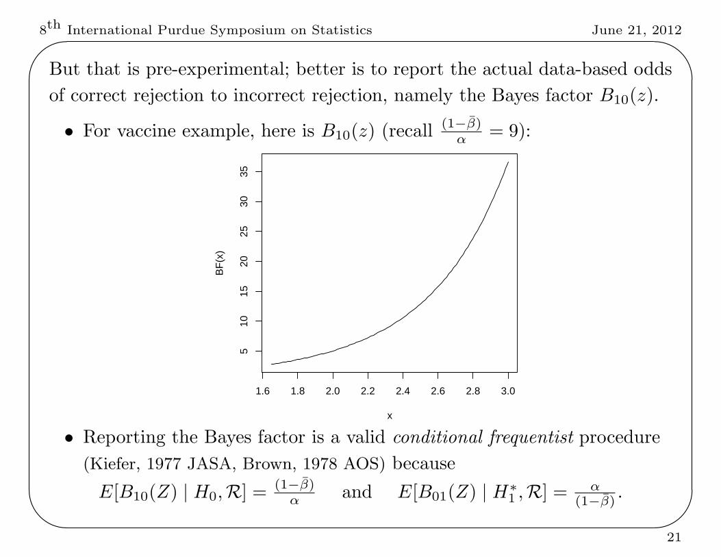
But that is pre-experimental; better is to report the actual data-based odds
of correct rejection to incorrect rejection, namely the Bayes factor B10(z).
• For vaccine example, here is B10(z) (recall(1−β̄)
α = 9):
1.6 1.8 2.0 2.2 2.4 2.6 2.8 3.0
510
1520
2530
35
x
BF
(x)
• Reporting the Bayes factor is a valid conditional frequentist procedure
(Kiefer, 1977 JASA, Brown, 1978 AOS) because
E[B10(Z) | H0,R] = (1−β̄)α and E[B01(Z) | H∗
1 ,R] = α(1−β̄)
.
21

8th International Purdue Symposium on Statistics June 21, 2012'
&
$
%
A General Bound
Robust Bayesian theory suggests a general and simple way to calibrate
p-values. (Sellke, Bayarri and Berger, 2001 Am. Stat.).
• A proper p-value satisfies H0 : p(X) ∼ Uniform(0, 1).
• Consider testing this versus H1 : p ∼ f(p), where Y = − log(p) has a
decreasing failure rate (a natural non-parametric alternative).
• Theorem 1 If p < e−1, B01 ≥ −e p log(p).
• An analogous lower bound on the conditional Type I frequentist error is
α(p) ≥ (1 + [−e p log(p)]−1)−1 .
p .2 .1 .05 .01 .005 .001 .0001 .00001
−ep log(p) .879 .629 .409 .123 .072 .0189 .0025 .00031
α(p) .465 .385 .289 .111 .067 .0184 .0025 .00031
22

8th International Purdue Symposium on Statistics June 21, 2012'
&
$
%Figure 4: J.P. Ioannides: Am J Epidemiol 2008;168:374–383
23

8th International Purdue Symposium on Statistics June 21, 2012'
&
$
%24
8th International Purdue Symposium on Statistics June 21, 2012'
&
$
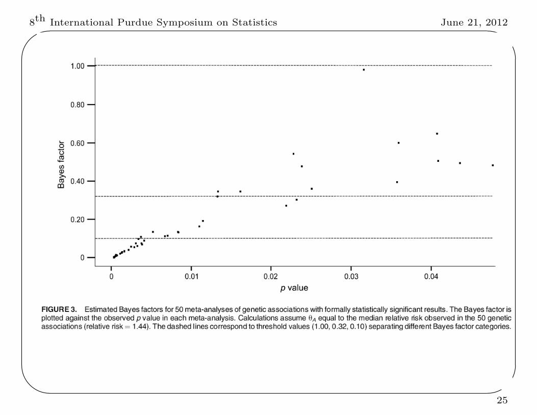
%25

8th International Purdue Symposium on Statistics June 21, 2012'
&
$
%Figure 5: Elgersma and Green (2011): α(p) versus observed p-values for 314
articles in Ecology in 2009.
26

8th International Purdue Symposium on Statistics June 21, 2012'
&
$
%
The Bayesian Approach to Multiple Testing
Key Fact: Bayesian analysis deals with multiplicity testing solely through
the assignment of prior probabilities to models or hypotheses.
Example: Multiple Testing under Exclusivity
Suppose one is testing mutually exclusive hypotheses Hi, i = 1, . . . ,m, so
each hypothesis is a separate model.
If the hypotheses are viewed as exchangeable, choose P (Hi) = 1/m.
Example: 1000 energy channels are searched for a signal:
• if the signal is known to exist and occupy only one channel, but no channel is
theoretically preferred, each channel can be assigned prior probability 0.001.
• if the signal is not known to exist, prior probability 1/2 should be given to
‘no signal,’ and probability 0.0005 to each channel.
This is the Bayesian solution regardless of the structure of the data. In
contrast, frequentist solutions depend strongly on feature of the data such as
their dependence structure, making them challenging to implement.
27

8th International Purdue Symposium on Statistics June 21, 2012'
&
$
%
Example: Genome-wide Association Studies (GWAS)
• Early genomic epidemiological studies almost universally failed to
replicate (estimates of the replication rate are as low as 1%), because
they were doing multiple testing at ‘ordinary p-values’.
• A very influential paper in Nature (2007) by the Wellcome Trust Case
Control Consortium proposed cutoff p < 5× 10⁻⁷ (−ep log(p) = 2× 10⁻⁵)
– Found 21 genome/disease associations; 20 have been replicated.
• Bayes argument for the cutoff:
– Pre-experimental ‘odds of true positive to false positive’
= prior odds× (1−β̄)α .
– For the GWAS study, they choose prior odds = 1100,000
and (1− β̄) = 0.5,
giving odds of 10 : 1 in favor of a true positive if α = 5× 10⁻⁷.
(They stated the prior odds could vary by a factor of 10.)
– The article also argued that it is better to just compute the Bayes factors
B10(z), and the posterior odds = prior odds×B10(z) . These ranged
between 110
and 1068 for the 21 claimed associations.
28

8th International Purdue Symposium on Statistics June 21, 2012'
&
$
%
Summary 1. There is a lack of recognition that better statisticsis the solution to much of the reproducibility problem
The extent of the problem:
• Dozens (hundreds) of articles addressing the problem; few say much
about statistics (except those written by statisticians).
• Few journals adequately police the statistical analyses in their papers.
“What’s the difference between ignorance and apathy?”
“I don’t know and I don’t care.”
• An extreme illustration - The Decline Effect (see “The Truth Wears Off,”
by Jonah Lehrer in the New Yorker, 2010):
– This is the well-observed phenomenon that as more studies come in on
something, the effect size declines.
– This has been hypothesized to be a law of nature, like the uncertainty
principle; scientists observing nature change nature.
29

8th International Purdue Symposium on Statistics June 21, 2012'
&
$
%
Summary 2: How Bayesian analysis can help
• While it may not be possible to replace p-values with Bayes factors,
one can at least replace them with
– −ep log(p), termed the lower bound on the odds of no effect to there
being an effect; or
– [1 + (−ep log(p))−1]−1, termed the lower bound on the conditional
frequentist Type 1 error.
• With Bayesian analysis there is no debate about a penalty for multiple
tests, since prior probabilities are transparent.
• There is then no optional stopping issue; formal Bayesian answers do
not depend on the stopping rule (although −ep log(p) might).
• There is then a systematic way to deal with multiple statistical
analyses, through Bayesian model averaging.
30

8th International Purdue Symposium on Statistics June 21, 2012'
&
$
%
Summary 3. Other efforts to address thereproducibility issue*
• There have been a variety of efforts to establish protocols for scientific
investigation:
– Pre-experimental statements of intent and plan.
– Documentation of all manipulations of data and all analyses attempted
(e.g. Sweave); at a minimum, give the data.
– Protocols for allowed methods of analysis.
• Efforts to allow publication of all results, positive or not.
• Optimal solution is to convince the science funding agencies to include
statisticians on research teams, or at least provide funds for the data
analysis, but this would require a radical expansion of statistics.
• Should statistical societies (as opposed to individual statisticians)
police systemic bad statistical practice?
*“I was going to buy a copy of The Power of Positive Thinking, and then I
thought: What the hell good would that do?” –Ronnie Shakes
31

8th International Purdue Symposium on Statistics June 21, 2012'
&
$
%
George Casella, 1951-2012• Being at the forefront of promoting
good statistical practice
• Testing and p-values: papers on
– understanding and proper use
of p-values
– conditional frequentist methods
– objective Bayesian alternatives
• Bayesian multiplicity control
– “Objective Bayesian analysis of
multiple changepoints for lin-
ear models” (Bayesian Statis-
tics, 2007)
– “Consistency of objective Bayes
factors as the model dimension
grows” (AOS, 2010)
– Many genomics papers
– Software (BAMD)
32