Embed Size (px)
Citation preview

PACIFIC EARTHQUAKE ENGINEERING RESEARCH CENTER
Performance Modeling Strategies for Modern Reinforced
Concrete Bridge Columns
Michael P. Berry
Montana State University, Bozeman
and
Marc O. Eberhard
University of Washington, Seattle
PEER 2007/07APRIL 2008

Performance Modeling Strategies forModern Reinforced Concrete Bridge
Columns
Michael P. Berry
Department of Civil Engineering
Montana State University, Bozeman
Marc O. Eberhard
Department of Civil and Environmental Engineering
University of Washington, Seattle
PEER Report 2007/07
Pacific Earthquake Engineering Research Center
College of Engineering
University of California, Berkeley
April 2008

ABSTRACT
It is important to characterize the performance of bridges during earthquakes because they are
integral components of transportation networks. Loss of bridge function can have severe eco-
nomic consequences, and consequences to life safety when bridges are critical links in lifelines to
emergency facilities, which are particularly important after a disasters. Although damage to other
elements can have economic and life-safety impacts, reinforced concrete columns are often the
most vulnerable elements in a bridge, and column failure can have catastrophic consequences.
The objective of this project was to develop column-modeling strategies to accurately model
column behavior under seismic loading, including global and local forces and deformations, as well
as progression of damage. The models were calibrated using the observed cyclic force-deformation
responses and damage progression observations of 37 tests of spiral-reinforced columns represen-
tative of modern bridge construction. This research resulted in (1) a standardized discretization
scheme for fiber cross sections; (2) a calibrated distributed-plasticity column modeling strategy
including deformation components for bond-slip and shear deformations; (3) a calibrated lumped-
plasticity column modeling strategy with recommendations for effective elastic-stiffness properties
and plastic-hinge lengths; (4) the identification of inaccuracies of standard cyclic material models;
(5) the implementation and evaluation of improved cyclic material models; (6) a series of dam-
age equations to predict two flexural damage states with three engineering demand parameters;
(7) the evaluation of the proposed modeling strategies when applied to complex structural models
(two-column bent, and biaxial shake-table specimen).
This effort is an important step toward implementing performance-based earthquake engi-
neering for modern reinforced concrete bridges.
iii

ACKNOWLEDGMENTS
This work was supported primarily by the Earthquake Engineering Research Centers Program of
the National Science Foundation under award number EEC- 9701568 through the Pacific Earth-
quake Engineering Research Center (PEER). Any opinions, findings, and conclusions or recom-
mendations expressed in this material are those of the author(s) and do not necessarily reflect those
of the National Science Foundation.
The authors would like to thank Professors Dawn Lehman, John Stanton, Laura Lowes, and
Greg Miller for their invaluable advice and assistance.
Finally, the author would like to thank his friends Dylan Freytag, Aaron Sterns, Nilanjan
Mitra, Nathan McBride, Mark Gallik, and Tyler Ranf; his family, Sandy, Tim, Tim Jr., Shelley,
Dave, Wendell, Candy, Mark, Casey, and Tony; and his wife Deanna for their patience and support
throughout this research project.
iv

CONTENTS
ABSTRACT . . . . . . . . . . . . . . . . . . . . . . . . . . . . . . . . . . . . . . . . . . ii
ACKNOWLEDGMENTS . . . . . . . . . . . . . . . . . . . . . . . . . . . . . . . . . . . iv
TABLE OF CONTENTS . . . . . . . . . . . . . . . . . . . . . . . . . . . . . . . . . . . v
LIST OF FIGURES . . . . . . . . . . . . . . . . . . . . . . . . . . . . . . . . . . . . . . ix
LIST OF TABLES . . . . . . . . . . . . . . . . . . . . . . . . . . . . . . . . . . . . . . . xiii
1 INTRODUCTION . . . . . . . . . . . . . . . . . . . . . . . . . . . . . . . . . . . . . 11.1 Context . . . . . . . . . . . . . . . . . . . . . . . . . . . . . . . . . . . . . . . . 11.2 Objective . . . . . . . . . . . . . . . . . . . . . . . . . . . . . . . . . . . . . . . 21.3 Bridge Column Data . . . . . . . . . . . . . . . . . . . . . . . . . . . . . . . . . 31.4 Scope of Project . . . . . . . . . . . . . . . . . . . . . . . . . . . . . . . . . . . . 4
2 DISCRETIZATION STRATEGIES FOR FIBER SECTIONS . . . . . . . . . . . . . 92.1 Fiber Model . . . . . . . . . . . . . . . . . . . . . . . . . . . . . . . . . . . . . . 92.2 Material Constitutive Relationships . . . . . . . . . . . . . . . . . . . . . . . . . . 92.3 Uniform Radial Section-Discretization Strategy . . . . . . . . . . . . . . . . . . . 132.4 Nonuniform Radial Discretization Strategy . . . . . . . . . . . . . . . . . . . . . 182.5 Summary . . . . . . . . . . . . . . . . . . . . . . . . . . . . . . . . . . . . . . . 19
3 DEVELOPMENT OF DISTRIBUTED-PLASTICITY COLUMN MODEL . . . . . 233.1 Nonlinear Force-Based Beam-Column Element (Flexure) . . . . . . . . . . . . . . 243.2 Bond Slip Displacement Model . . . . . . . . . . . . . . . . . . . . . . . . . . . . 383.3 Shear-Displacement Model . . . . . . . . . . . . . . . . . . . . . . . . . . . . . . 403.4 OpenSees Implementation . . . . . . . . . . . . . . . . . . . . . . . . . . . . . . 413.5 Summary . . . . . . . . . . . . . . . . . . . . . . . . . . . . . . . . . . . . . . . 42
4 CALIBRATION OF DISTRIBUTED-PLASTICITY COLUMN MODEL . . . . . . 454.1 Column Data . . . . . . . . . . . . . . . . . . . . . . . . . . . . . . . . . . . . . 464.2 Steel Strain-Hardening Ratio Calibration . . . . . . . . . . . . . . . . . . . . . . . 474.3 Bond-Strength Model Calibration . . . . . . . . . . . . . . . . . . . . . . . . . . 474.4 Optimization Strategy for Remaining Model Parameters . . . . . . . . . . . . . . . 484.5 Optimization Results . . . . . . . . . . . . . . . . . . . . . . . . . . . . . . . . . 51
v

4.6 Model Evaluation . . . . . . . . . . . . . . . . . . . . . . . . . . . . . . . . . . . 544.7 Sensitivity Analyses . . . . . . . . . . . . . . . . . . . . . . . . . . . . . . . . . . 604.8 Evaluation with Database of Bridge Columns . . . . . . . . . . . . . . . . . . . . 644.9 Summary . . . . . . . . . . . . . . . . . . . . . . . . . . . . . . . . . . . . . . . 69
5 DEVELOPMENT OF LUMPED-PLASTICITY COLUMN MODEL . . . . . . . . 715.1 Model Formulations . . . . . . . . . . . . . . . . . . . . . . . . . . . . . . . . . . 715.2 Yield Displacement . . . . . . . . . . . . . . . . . . . . . . . . . . . . . . . . . . 735.3 Moment-Curvature Response . . . . . . . . . . . . . . . . . . . . . . . . . . . . . 775.4 Plastic-Hinge Lengths . . . . . . . . . . . . . . . . . . . . . . . . . . . . . . . . . 775.5 OpenSees Implementation . . . . . . . . . . . . . . . . . . . . . . . . . . . . . . 785.6 Summary . . . . . . . . . . . . . . . . . . . . . . . . . . . . . . . . . . . . . . . 80
6 CALIBRATION OF LUMPED-PLASTICITY COLUMN MODEL . . . . . . . . . 816.1 Measures of Accuracy . . . . . . . . . . . . . . . . . . . . . . . . . . . . . . . . 816.2 Column Stiffness . . . . . . . . . . . . . . . . . . . . . . . . . . . . . . . . . . . 826.3 Calibration of Plastic-Hinge Length . . . . . . . . . . . . . . . . . . . . . . . . . 876.4 Model Evaluation . . . . . . . . . . . . . . . . . . . . . . . . . . . . . . . . . . . 926.5 Summary . . . . . . . . . . . . . . . . . . . . . . . . . . . . . . . . . . . . . . . 97
7 EVALUATION OF CYCLIC RESPONSE . . . . . . . . . . . . . . . . . . . . . . . . 997.1 Cyclic Response of Materials . . . . . . . . . . . . . . . . . . . . . . . . . . . . . 997.2 Measures of Accuracy . . . . . . . . . . . . . . . . . . . . . . . . . . . . . . . . 1007.3 Evaluation of Distributed-Plasticity
Column-Modeling Strategy . . . . . . . . . . . . . . . . . . . . . . . . . . . . . . 1017.4 Evaluation of Lumped-Plasticity Column-Modeling Strategy . . . . . . . . . . . . 1057.5 Summary . . . . . . . . . . . . . . . . . . . . . . . . . . . . . . . . . . . . . . . 112
8 IMPROVED CYCLIC MATERIAL MODELS . . . . . . . . . . . . . . . . . . . . . 1178.1 Calibration of Mohle and Kunnath (2006) Steel Model . . . . . . . . . . . . . . . 1178.2 Imperfect Crack Closure . . . . . . . . . . . . . . . . . . . . . . . . . . . . . . . 1238.3 Summary . . . . . . . . . . . . . . . . . . . . . . . . . . . . . . . . . . . . . . . 128
9 COLUMN FLEXURAL DAMAGE . . . . . . . . . . . . . . . . . . . . . . . . . . . 1319.1 Estimates Based on Drift Ratio . . . . . . . . . . . . . . . . . . . . . . . . . . . . 1319.2 Damage Estimates Based on Plastic Rotation . . . . . . . . . . . . . . . . . . . . 1399.3 Damage Estimates Based on Strain . . . . . . . . . . . . . . . . . . . . . . . . . . 1489.4 Comparison of Damage Estimates . . . . . . . . . . . . . . . . . . . . . . . . . . 161
vi
10 APPLICATION OF COLUMN- MODELING STRATEGY TO MORE COMPLEXSTRUCTURAL MODELS . . . . . . . . . . . . . . . . . . . . . . . . . 163
10.1 Column Bent Tests . . . . . . . . . . . . . . . . . . . . . . . . . . . . . . . . . . 16310.2 Shake-Table Tests . . . . . . . . . . . . . . . . . . . . . . . . . . . . . . . . . . . 170
11 SUMMARY AND CONCLUSIONS . . . . . . . . . . . . . . . . . . . . . . . . . . . 18711.1 Cross-Section Modeling . . . . . . . . . . . . . . . . . . . . . . . . . . . . . . . 18711.2 Envelope Response of Distributed-Plasticity Column-Modeling Strategy . . . . . . 18811.3 Envelope Response of Lumped-Plasticity
Column-Modeling Strategy . . . . . . . . . . . . . . . . . . . . . . . . . . . . . . 18911.4 Cyclic Response of Modeling Strategies with Standard
Material Models . . . . . . . . . . . . . . . . . . . . . . . . . . . . . . . . . . . . 19011.5 Improved Cyclic Material Models . . . . . . . . . . . . . . . . . . . . . . . . . . 19111.6 Column Flexural Damage . . . . . . . . . . . . . . . . . . . . . . . . . . . . . . . 19211.7 Application of Column-Modeling Strategies to More Complex Structures . . . . . 19311.8 Recommendations for Further Work . . . . . . . . . . . . . . . . . . . . . . . . . 194
REFERENCES . . . . . . . . . . . . . . . . . . . . . . . . . . . . . . . . . . . . . . . . 195
vii

LIST OF FIGURES
Fig. 2.1 Typical fiber discretization, nrc = 7,nt
c = 18,nru = 2,nt
u = 18 . . . . . . . . 10Fig. 2.2 Reinforcing steel material model . . . . . . . . . . . . . . . . . . . . . . . 11Fig. 2.3 Concrete material models . . . . . . . . . . . . . . . . . . . . . . . . . . 12Fig. 2.4 Unidirectional section discretization . . . . . . . . . . . . . . . . . . . . . 13Fig. 2.5 Recommended configuration, nt
c = 20, nrc = 10, nt
u = 20 and nru = 1 . . . . 15
Fig. 2.6 Effect of nrc on m-! accuracy . . . . . . . . . . . . . . . . . . . . . . . . . 16
Fig. 2.7 Effect of ntc on m-! accuracy . . . . . . . . . . . . . . . . . . . . . . . . . 16
Fig. 2.8 Effect of nru on m-! accuracy . . . . . . . . . . . . . . . . . . . . . . . . . 17
Fig. 2.9 Effect of ntu on m-! accuracy . . . . . . . . . . . . . . . . . . . . . . . . . 17
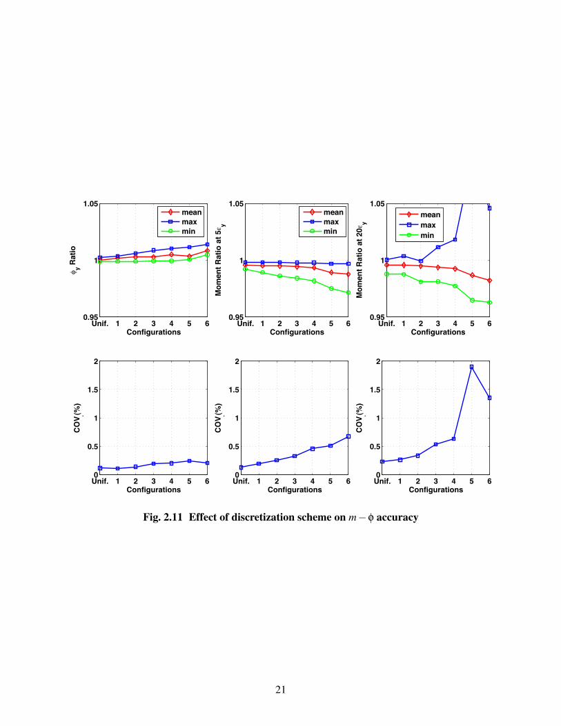
Fig. 2.10 Configuration types . . . . . . . . . . . . . . . . . . . . . . . . . . . . . . 20Fig. 2.11 Effect of discretization scheme on m−! accuracy . . . . . . . . . . . . . 21
Fig. 3.1 Distributed-plasticity model with bond slip and shear components . . . . . 23Fig. 3.2 Force-deformation envelope with varying np (hardening) . . . . . . . . . . 26Fig. 3.3 Strain distributions for varying np (hardening) . . . . . . . . . . . . . . . 26Fig. 3.4 Force-deformation envelope with varying np (plateau) . . . . . . . . . . . 27Fig. 3.5 Strain distributions for varying np (plateau) . . . . . . . . . . . . . . . . . 27Fig. 3.6 Force-deformation envelope with varying np (softening) . . . . . . . . . . 28Fig. 3.7 Strain distributions for varying np (softening) . . . . . . . . . . . . . . . . 28Fig. 3.8 Force-deformation and strain dependency on np (cantilever) . . . . . . . . 30Fig. 3.9 Force-deformation and strain dependency on np (double curvature) . . . . 31Fig. 3.10 Curvature response for typical column with varying strain-hardening ratio . 35Fig. 3.11 Curvature response for typical column with degrading section response . . 36Fig. 3.12 Curvature response for typical column with hardening section response . . 37Fig. 3.13 Bond model illustration . . . . . . . . . . . . . . . . . . . . . . . . . . . 38Fig. 3.14 Stress-displacement envelope for typical anchor bar . . . . . . . . . . . . 39Fig. 3.15 Assumed compressive depth . . . . . . . . . . . . . . . . . . . . . . . . . 40Fig. 3.16 Comparison of calculated f-" envelopes . . . . . . . . . . . . . . . . . . . 44
Fig. 4.1 Measured and calculated stress-strain response of steel . . . . . . . . . . . 47Fig. 4.2 Bond-strength calibration . . . . . . . . . . . . . . . . . . . . . . . . . . 48Fig. 4.3 Effect of np on optimization surface . . . . . . . . . . . . . . . . . . . . . 52Fig. 4.4 Measured and calculated force-" envelopes . . . . . . . . . . . . . . . . . 56Fig. 4.5 Components of total deflection . . . . . . . . . . . . . . . . . . . . . . . . 57Fig. 4.6 Measured and calculated average strains (up to "
"y= 8) . . . . . . . . . . . 58
ix

Fig. 4.7 Measured and calculated average strains (up to ""y
= 3) . . . . . . . . . . . 59
Fig. 4.8 Effect of varying strain-hardening ratio (b) . . . . . . . . . . . . . . . . . 61Fig. 4.9 Effect of varying number of integration points (np) . . . . . . . . . . . . . 61Fig. 4.10 Effect of varying bond-strength ratio (#) . . . . . . . . . . . . . . . . . . . 62Fig. 4.11 Effect of varying bond compression depth (dcomp) . . . . . . . . . . . . . 62Fig. 4.12 Effect of varying shear-stiffness ratio ($) . . . . . . . . . . . . . . . . . . . 63Fig. 4.13 Effect of key properties on pushover error . . . . . . . . . . . . . . . . . . 65Fig. 4.14 Effect of key properties on stiffness ratio . . . . . . . . . . . . . . . . . . 66Fig. 4.15 Effect of key properties on moment ratio . . . . . . . . . . . . . . . . . . 67Fig. 4.16 Effect of key properties on degradation error ratio . . . . . . . . . . . . . . 68
Fig. 5.1 Moment and curvature distributions . . . . . . . . . . . . . . . . . . . . . 72
Fig. 6.1 %g versus key column properties . . . . . . . . . . . . . . . . . . . . . . . 84Fig. 6.2 %sec versus key column properties . . . . . . . . . . . . . . . . . . . . . . 85
Fig. 6.3 Correlation between ld and fydb
l& . . . . . . . . . . . . . . . . . . . . . . . 87Fig. 6.4 Effect of key properties on pushover error . . . . . . . . . . . . . . . . . . 93Fig. 6.5 Effect of key properties on stiffness ratio . . . . . . . . . . . . . . . . . . 94Fig. 6.6 Effect of key properties on moment ratio . . . . . . . . . . . . . . . . . . 95Fig. 6.7 Effect of key properties on degradation error ratio . . . . . . . . . . . . . . 96
Fig. 7.1 Cyclic response of longitudinal reinforcing steel . . . . . . . . . . . . . . 100Fig. 7.2 Cyclic response of concrete . . . . . . . . . . . . . . . . . . . . . . . . . 100Fig. 7.3 Measured vs. calculated force-deformation responses for bridge subset . . 103Fig. 7.4 Error distribution for distributed-plasticity model . . . . . . . . . . . . . . 104Fig. 7.5 Force-deformation histories for column tests with min and max E f orce values105Fig. 7.6 Effect of maximum ductility on E f orce and Eenergy . . . . . . . . . . . . . . 106Fig. 7.7 Effect of key column properties on E f orce using distributed-plasticity model 107Fig. 7.8 Effect of key column properties on Eenergy using distributed-plasticity model108Fig. 7.9 Measured vs. calculated force-deformation responses for bridge subset . . 110Fig. 7.10 Error distribution for lumped-plasticity model . . . . . . . . . . . . . . . . 111Fig. 7.11 Force-deformation histories for column tests with min and max E f orce values112Fig. 7.12 Effect of maximum ductility on cyclic accuracy for lumped-plasticity model 113Fig. 7.13 Effect of key column properties on E f orce using lumped-plasticity model . 114Fig. 7.14 Effect of key column properties on Eenergy using lumped-plasticity model . 115
Fig. 8.1 Coffin and Manson parameters (based on Mohle and Kunnath, 2006) . . . 119Fig. 8.2 Effect of Coffin and Manson parameters on cyclic response of steel . . . . 120Fig. 8.3 Force-deformation response, Kunnath steel model . . . . . . . . . . . . . 122Fig. 8.4 Cyclic response of concrete with imperfect crack closure . . . . . . . . . . 125
x

Fig. 8.5 Strain history for demonstration of imperfect crack closure properties . . . 126Fig. 8.6 Effect r on concrete stress-strain response . . . . . . . . . . . . . . . . . . 126Fig. 8.7 Effect effect cmax on concrete stress-strain response . . . . . . . . . . . . . 127Fig. 8.8 Effect of r on overall model accuracy (lumped-plasticity, Kunnath steel) . . 128Fig. 8.9 Effect of cmax on overall model accuracy (lumped-plasticity, Kunnath steel) 129
Fig. 9.1 Key flexural damage states (Ranf, 2006) . . . . . . . . . . . . . . . . . . . 132Fig. 9.2 Fragility curves for cover spalling, bar buckling, and bar fracture . . . . . . 135Fig. 9.3 Effect of key properties on accuracy of drift-ratio spalling equations. . . . . 136Fig. 9.4 Effect of key properties on accuracy of drift-ratio buckling equations. . . . 137Fig. 9.5 Effect of key properties on accuracy of drift-ratio bar-fracture equations. . 138Fig. 9.6 Fragility curves for cover spalling and bar buckling using plastic rotation . 141Fig. 9.7 Effect of key properties on accuracy of plastic-rotation spalling equations. . 142Fig. 9.8 Fragility curves for bar buckling using plastic rotation . . . . . . . . . . . 146Fig. 9.9 Effect of key properties on accuracy of plastic-rotation bar-buckling equation147Fig. 9.10 Fragility curves for bar fracture using plastic rotation . . . . . . . . . . . . 149Fig. 9.11 Effect of key properties on accuracy of plastic-rotation bar-fracture equation 150Fig. 9.12 Effect of effective confinement ratio on 'sp . . . . . . . . . . . . . . . . . 152Fig. 9.13 Fragility curves for cover spalling and bar buckling using longitudinal strain 152Fig. 9.14 Effect of key properties on accuracy of strain estimates of cover spalling . . 155Fig. 9.15 Effect of effective confinement ratio on 'bb . . . . . . . . . . . . . . . . . 156Fig. 9.16 Fragility curves for bar buckling using longitudinal tensile strain . . . . . . 156Fig. 9.17 Effect of key properties on accuracy of strain estimates of bar buckling . . 157Fig. 9.18 Effect of effective confinement ratio on 'b f . . . . . . . . . . . . . . . . . 158Fig. 9.19 Fragility curves for bar fracture using longitudinal tensile strain . . . . . . 159Fig. 9.20 Effect of key column properties on accuracy of strain estimates of bar fracture160
Fig. 10.1 Test setup . . . . . . . . . . . . . . . . . . . . . . . . . . . . . . . . . . . 164Fig. 10.2 Bent model with distributed-plasticity column-modeling strategy . . . . . . 166Fig. 10.3 Force-deformation response of bent, distributed-plasticity, standard steel . 167Fig. 10.4 Bent model with lumped-plasticity column-modeling strategy . . . . . . . 168Fig. 10.5 Force-deformation response of bent, lumped-plasticity, standard steel . . . 169Fig. 10.6 Force-deformation response of bent, lumped-plasticity, Mohle/Kunnath steel169Fig. 10.7 Column specimen and key dimensions (Hachem et al. 2003) . . . . . . . . 172Fig. 10.8 Base-acceleration records for test specimens . . . . . . . . . . . . . . . . 173Fig. 10.9 Response spectra for base accelerations with a damping ratio of 5% . . . . 174Fig. 10.10 Modeling strategies for shake-table tests . . . . . . . . . . . . . . . . . . . 175Fig. 10.11 Measured to calculated maxima in the lat. direction at 1st design level . . . 177Fig. 10.12 Measured to calculated maxima in the long. direction at 1st design level . . 178
xi

Fig. 10.13 Measured to calculated maxima in the lat. direction at 1st maximum level . 179Fig. 10.14 Measured to calculated maxima in the long. direction at 1st maximum level 180Fig. 10.15 Comparison of measured and calculated residual displacements . . . . . . 181Fig. 10.16 Normalized residual displacement errors . . . . . . . . . . . . . . . . . . 183
xii

LIST OF TABLES
Table 1.1 Bridge column dataset . . . . . . . . . . . . . . . . . . . . . . . . . . . . 4
Table 2.1 Discretization study matrix . . . . . . . . . . . . . . . . . . . . . . . . . . 19
Table 4.1 Calibration parameter ranges for initial run . . . . . . . . . . . . . . . . . 50Table 4.2 Distributed-plasticity optimization results . . . . . . . . . . . . . . . . . . 51Table 4.3 Distributed-plasticity optimization results (np = 5, $ = 0.4 and dcomp = c) . 53Table 4.4 Accuracy statistics for envelope response of distributed-plasticity model . . 64
Table 5.1 Expected trends in % . . . . . . . . . . . . . . . . . . . . . . . . . . . . . 77
Table 6.1 Statistics of s.r. . . . . . . . . . . . . . . . . . . . . . . . . . . . . . . . . 83Table 6.2 Statistics of s.r. using % expressions . . . . . . . . . . . . . . . . . . . . . 86Table 6.3 Calibration parameter ranges for plastic-hinge length . . . . . . . . . . . . 88Table 6.4 Lumped-plasticity optimization results . . . . . . . . . . . . . . . . . . . 90Table 6.5 Comparison of lumped-plasticity models . . . . . . . . . . . . . . . . . . 91
Table 7.1 Cyclic response statistics for distributed-plasticity model . . . . . . . . . . 102Table 7.2 Cyclic response statistics for lumped-plasticity model . . . . . . . . . . . 106
Table 8.1 Cyclic response statistics (Kunnath steel with lumped-plasticity model) . . 121
Table 9.1 Key accuracy statistics of drift-ratio equations with bridge column dataset . 133Table 9.2 Results of plastic-rotation calibration . . . . . . . . . . . . . . . . . . . . 140Table 9.3 Results of plastic-rotation calibration . . . . . . . . . . . . . . . . . . . . 144Table 9.4 Results of plastic-rotation calibration . . . . . . . . . . . . . . . . . . . . 146Table 9.5 Cover-spalling estimates based on longitudinal compressive strain . . . . . 151Table 9.6 Buckling estimates based on longitudinal-reinforcement tensile strain . . . 153Table 9.7 Bar-fracture estimates based on longitudinal-reinforcement tensile strain . 158Table 9.8 Comparison of damage estimates . . . . . . . . . . . . . . . . . . . . . . 161
Table 10.1 Geometric properties of the Purdue bent . . . . . . . . . . . . . . . . . . . 165Table 10.2 Measured material properties for the Purdue bent . . . . . . . . . . . . . . 165Table 10.3 Accuracy statistics for column-modeling strategies . . . . . . . . . . . . . 166Table 10.4 Damage estimates for purdue bent test . . . . . . . . . . . . . . . . . . . . 170Table 10.5 Properties of shake-table specimens . . . . . . . . . . . . . . . . . . . . . 171Table 10.6 Test matrix with pga for 1st design level and 1st maximum level . . . . . . 171Table 10.7 Modeling variations for shake-table specimens . . . . . . . . . . . . . . . 176Table 10.8 Summary of spalling estimates . . . . . . . . . . . . . . . . . . . . . . . . 185Table 10.9 Summary of bar-buckling estimates . . . . . . . . . . . . . . . . . . . . . 185
xiii

Table 11.1 Accuracy statistics for envelope response of column-modeling strategies . . 189Table 11.2 Accuracy statistics for cyclic response of column-modeling strategies . . . 191Table 11.3 Comparison of damage estimates . . . . . . . . . . . . . . . . . . . . . . 192Table 11.4 Accuracy statistics for bent specimen . . . . . . . . . . . . . . . . . . . . 193
xiv

1 Introduction
1.1 CONTEXT
Current building codes and modern engineering practice address the issues of collapse prevention
and life safety by conservatively predicting nominal demands and strengths of structural members,
but provide little indication of the actual state of a structure after an earthquake. After an earth-
quake, a building or bridge may still be standing, but structural and nonstructural members may be
damaged, resulting in costly repairs. The economic losses due to downtime may even be larger.
In contrast to current codes, performance-based earthquake engineering (PBEE) attempts
to explicitly predict damage states and assess the probability of reaching multiple levels of dam-
age. PBEE has the potential to improve structural engineering practice by providing engineers
the capability of designing structures to achieve a variety of performance levels. The impact of
implementing PBEE goes beyond improving engineering practice and extends to a wide range of
decision making. The potential impact of PBEE is summarized in Pacific Earthquake Engineering
Research Center’s (PEER) mission statement.
This approach is aimed at improving decision-making about seismic risk by making
the choice of performance goals and the tradeoffs that they entail apparent to facility
owners and society at large. The approach has gained worldwide attention in the
past ten years with the realization that urban earthquakes in developed countries -
Loma Prieta, Northridge, and Kobe - impose substantial economic and societal risks
above and beyond potential loss of life and injuries. By providing quantitative tools for
characterizing and managing these risks, performance-based earthquake engineering
serves to address diverse economic and safety needs. (http://peer.berkeley.edu)
1

Reinforced concrete structures are particularly vulnerable to earthquakes. Excessive defor-
mations can result in spalling of cover concrete, buckling of longitudinal reinforcement, reduction
of flexural capacity, bar fracture, and eventually, structural collapse. Although damage to other ele-
ments can have economic and life-safety impacts, columns are often the most vulnerable elements
in a structure, and column failure can have catastrophic consequences.
To quantitatively implement PBEE for reinforced concrete columns, it is necessary to predict
deformation demands on columns at the onset of particular damage states. Berry and Eberhard
(2003) developed practical empirical models that predict the drift ratios at which cover concrete
spalls and longitudinal bars buckle in reinforced concrete columns, given a column geometry,
transverse reinforcement, and axial load. The models were calibrated with existing experimental
results from the UW-PEER reinforced concrete column performance database, which documents
the performance of over 400 columns (Berry et al. 2004).
The drift-ratio approach provides a simple means of estimating damage displacements (which
is essential to engineering practice), but it has significant limitations. This approach neglects the
effects of cycling on damage and it is difficult to implement for columns with biaxial bending,
variable axial loads or variable shear spans. More versatile and detailed models are needed to
overcome these limitations.
The availability of increasingly powerful computers provides researchers and engineers with
the opportunity to implement numerically intensive modeling strategies that could not have been
considered until recently. In particular, enhanced fiber beam-column elements have been developed
to model the nonlinear behavior of reinforced concrete structures under cyclic loads. Previous re-
searchers have used these simulation models to predict the response of ductile reinforced concrete
columns, but none of these modeling strategies have been calibrated with a large database to repro-
duce force-deformation behavior and damage progression. The absence of model calibration has
made it difficult to evaluate the impact of proposed improvements in modeling methodologies.
1.2 OBJECTIVE
The objective of this project is to develop, calibrate, and evaluate column-modeling strategies that
are capable of accurately modeling column behavior under seismic loading, including global and
local deformations, as well as progression of damage. The focus of this research will be on ductile
2

spiral-reinforced bridge columns, for which shear failure is not a consideration.
1.3 BRIDGE COLUMN DATA
The UW-PEER reinforced concrete column test database (Berry et al. 2004) provides a unique
opportunity to evaluate and calibrate column-modeling strategies. The database documents col-
umn geometry, material properties, and reinforcement details. It also includes the digital force-
displacement histories, and the observed displacements at the onset of multiple damage states.
For this study on ductile spiral-reinforced columns, the columns from the database were
screened to eliminate columns that are not representative of modern bridge construction. The
database was screened using the following criteria.
· P/Ag f ′c ≤ 0.30
· (e f f = (s fys/ f ′c ≥ 0.05
· (l ≤ 0.04
· S/db ≤ 6
· cover/D≤ 0.10
· Availability of observed displacements at onset of cover spalling, bar buckling, or bar frac-
ture
where: P is the axial load, Ag is the gross cross-sectional area, f ′c is the concrete compressive
strength, (s is the transverse reinforcement ratio, fys is the yield stress of the spiral reinforcement,
(l is the longitudinal-reinforcement ratio, S is the spacing of the spiral reinforcement, db is the
diameter of the longitudinal reinforcement, cover is the distance from column face to the transverse
reinforcement, and D is the diameter of the column.
The 37 column tests considered in this study are listed in Table 1.1. The reported drift ratios
at the onset of cover spalling ("sp/L), bar buckling ("bb/L), bar fracture ("b f /L) are included in
the table along with key properties of the columns.
3

Table 1.1 Bridge column dataset
Reference Designation L L/D (e f f P/Ag f ′c (l S/db "sp/L "bb/L "b f /L(mm) (%) (%) (%)
Munro et al. (1976) No. 1 2730 5.5 0.13 0.00 0.026 1.85 1.39 - -Ghee et al. (1981) No. 1 1600 4.0 0.09 0.20 0.024 2.50 0.94 3.75 3.75Pontangaroa et al. (1979) No. 1 1200 2.0 0.08 0.23 0.024 3.13 0.83 - -Wong et al. (1990) No. 1 800 2.0 0.11 0.19 0.032 3.75 0.75 5.18 -Stone and Cheok (1989) Flexure 9140 6.0 0.09 0.07 0.020 2.07 1.96 5.89 5.89Stone and Cheok (1989) Shear 4570 3.0 0.19 0.07 0.020 1.26 - 6.24 7.79Cheok and Stone (1986) N1 750 3.0 0.26 0.10 0.020 1.27 2.57 11.00 10.29Cheok and Stone (1986) N2 750 3.0 0.27 0.21 0.020 1.27 - 6.21 7.45Cheok and Stone (1986) N3 1500 6.0 0.13 0.10 0.020 2.07 3.41 7.38 6.83Cheok and Stone (1986) N4 750 3.0 0.26 0.10 0.020 1.27 2.84 7.11 7.11Cheok and Stone (1986) N5 750 3.0 0.26 0.20 0.020 1.27 2.58 6.96 6.44Cheok and Stone (1986) N6 1500 6.0 0.14 0.10 0.020 2.07 2.24 4.77 6.72Kunnath et al. (1997) No. A2 1372 4.5 0.14 0.09 0.020 2.00 - 4.70 -Kunnath et al. (1997) No. A3 1372 4.5 0.14 0.09 0.020 2.00 1.97 - -Kunnath et al. (1997) No. A7 1372 4.5 0.13 0.09 0.020 2.00 1.46 5.83 -Kunnath et al. (1997) No. A8 1372 4.5 0.13 0.09 0.020 2.00 2.33 5.83 -Kunnath et al. (1997) No. A9 1372 4.5 0.13 0.09 0.020 2.00 - 4.59 -Kunnath et al. (1997) No. A10 1372 4.5 0.15 0.10 0.020 2.00 2.33 6.61 -Kunnath et al. (1997) No. A11 1372 4.5 0.15 0.10 0.020 2.00 3.64 - 7.65Kunnath et al. (1997) No. A12 1372 4.5 0.15 0.10 0.020 2.00 3.64 5.90 -Hose et al. (1997) No. SRPH1 3660 6.0 0.09 0.15 0.027 2.56 1.64 8.74 8.74Vu et al. (1998) No. NH3 910 2.0 0.13 0.15 0.024 3.78 2.06 5.49 -Kowalsky et al. (1999) No. FL3 3656 8.0 0.12 0.30 0.036 4.79 - 9.08 9.08Lehman and Moehle (2000) No.415 2438 4.0 0.14 0.07 0.015 2.00 1.56 5.29 7.30Lehman and Moehle (2000) No.815 4877 8.0 0.14 0.07 0.015 2.00 2.73 9.12 9.12Lehman and Moehle (2000) No.1015 6096 10.0 0.14 0.07 0.015 2.00 3.13 10.42 10.42Lehman and Moehle (2000) No.407 2438 4.0 0.14 0.07 0.008 2.00 1.56 5.21 5.21Lehman and Moehle (2000) No.430 2438 4.0 0.14 0.07 0.030 2.00 1.56 7.30 -Lehman and Moehle (2000) No.328 1829 3.0 0.16 0.09 0.027 1.33 1.64 7.27 7.22Lehman and Moehle (2000) No.828 4877 8.0 0.16 0.09 0.027 1.33 3.65 12.30 -Lehman and Moehle (2000) No.1028 6096 10.0 0.16 0.09 0.027 1.33 4.17 14.58 -Henry and Mahin (1999) No. 415p 2438 4.0 0.12 0.12 0.015 2.00 - 5.21 5.54Henry and Mahin (1999) No. 415s 2438 4.0 0.06 0.06 0.015 4.00 - 5.21 -Moyer and Kowalsky (2001) No.1 2438 5.3 0.12 0.04 0.020 4.00 3.02 6.15 7.66Moyer and Kowalsky (2001) No.2 2438 5.3 0.11 0.04 0.020 4.00 2.29 10.73 12.29Moyer and Kowalsky (2001) No.3 2438 5.3 0.12 0.04 0.020 4.00 3.02 10.74 -Moyer and Kowalsky (2001) No.4 2438 5.3 0.11 0.04 0.020 4.00 3.02 13.14 -
Statistics n 37 37 37 37 37 37 31 33 31Mean 2458 4.8 0.14 0.11 0.021 2.35 2.33 7.39 7.62COV 0.75 0.4 0.35 0.57 0.25 0.42 0.39 0.37 0.26Min 750 2.0 0.06 0.00 0.008 1.26 0.75 3.75 3.75Max 9140 10.0 0.27 0.30 0.036 4.79 4.17 14.58 12.29
1.4 SCOPE OF PROJECT
Two column-modeling strategies are developed, calibrated, and evaluated in this report. One
method utilizes the combination of a force-based beam-column element (flexural deformations)
with elastic shear deformations and a zero-length bond-slip section. A second method utilizes
lumped-plasticity theory in which nonlinear deformations are concentrated in a plastic hinge. The
following describes the key aspects of the section modelling strategy, the distributed-plasticity
modeling strategy, and the lumped-plasticity modeling strategy addressed in this research.
1.4.1 Discretization Strategies for Fiber Cross Sections
Both column-modeling strategies use fiber sections to model section response. Two aspects of
fiber-section modeling are discussed in Chapter 2.
4

Material Models. Numerous material constitutive models are available to model the monotonic
and cyclic responses of the concrete and steel components of a reinforced concrete column.
In this study, key modeling parameters are calibrated for the Giuffre-Menegotto-Pinto steel
model (Taucer et al. 1991), the Mander et al. (1988) concrete model, and a new steel
model proposed by Mohle and Kunnath (2006), which includes softening due to fracture and
cycling.
Fiber-Section Discretization. Column cross sections can be discretized into small fibers using a
variety of schemes (e.g., unilateral discretization, radial discretization) to varying degrees of
mesh density. Two discretization strategies are evaluated, and recommendations are made
on the number of fibers needed to accurately model column section behavior.
1.4.2 Distributed-Plasticity Modeling Strategy
The distributed-plasticity modeling strategy is described and calibrated in chapters 3 and 4, respec-
tively. The following are key aspects of the proposed spread-plasticity column-modeling strategy
addressed by this study.
Number of integration points. The spread-plasticity column-modeling strategy requires the user to
select the number of integration points to use in the analysis. The effect of the number of
integration points on column model accuracy is studied and documented, and recommenda-
tions are made that balance model accuracy and efficiency.
Bond Slip Deformations and Shear Deformations. A standard fiber beam-column element formula-
tion assumes perfect bond between concrete and steel. To address this issues, a new zero-
length bond-slip model is developed for use with the spread-plasticity modeling strategy.
Shear Deformations. Shear deformations are neglected with a standard fiber beam-column element
formulation. Additional flexibility was added to the cross sections of the fiber beam-column
element to address this issue.
Strain Localization. The distributed-plasticity formulation is susceptible to strain localizations,
which lead to model inaccuracies when the column being modeled has a perfectly-plastic
or softening behavior. The limitations of this modeling strategy are highlighted, and recom-
mendations are made to assist in overcoming them.
5

1.4.3 Lumped-Plasticity Modeling Strategy
The lumped-plasticity column model is considered in chapters 5 and 6. The following are key
aspects of the lumped-plasticity column-modeling strategy addressed by this study.
Elastic Properties of Lumped-Plasticity Model. The use of lumped-plasticity models requires the
selection of effective section properties for the elastic portion of the column (e.g., EI). Rec-
ommendations are made for estimating these elastic properties, based on the accuracy of the
calculated column stiffness.
Plastic-Hinge Length of Lumped-Plasticity Model. Lumped-plasticity theory assumes that nonlin-
ear deformations are concentrated in plastic hinges. With this methodology, the length of
the plastic hinge is assumed to account for bond slip and shear deformations. A plastic-
hinge length that accurately predicts column force-deformation response as well as damage
progression is developed and evaluated.
1.4.4 Evaluation of Cyclic Response
The calculated cyclic response of the modeling strategies depend on the cyclic response of the
concrete and steel material constitutive models. The cyclic response of the proposed column-
modeling strategies, utilizing standard concrete and steel material models, are evaluated in Chapter
7. The cyclic response of the concrete was modeled according to a model proposed by Karsan and
Jirsa, whereas the steel was modeled according to a model proposed by Giuffre-Menegotto-Pinto.
1.4.5 Improved Cyclic Material Models
The cyclic modeling inaccuracies identified in Chapter 7 are addressed in Chapter 8. A steel
material model proposed by Mohle and Kunnath (2006), which accounts for degradation due to
cycling, is presented, calibrated, and evaluated. A concrete model that accounts for imperfect
crack closure is also developed and evaluated in this chapter.
1.4.6 Column Flexural Damage
A necessary step in implementing performance-based design in bridge columns is relating engi-
neering demand parameters (e.g., drift ratio, plastic rotation, longitudinal strain) to damage mea-
6

sures (e.g., cover spalling, longitudinal bar buckling, and bar fracture). Several methods for es-
timating the progression of damage in flexural columns are developed, evaluated, and compared
in Chapter 9. This chapter presents accuracy statistics and fragility curves for the various damage
states and engineering demand parameters.
1.4.7 Application of Column-Modeling Strategy to More Complex Structures
In chapters 4 and 6, the proposed column-modeling strategies were calibrated and evaluated by
comparing measured and calculated responses of single cantilever columns subjected to pseudo-
static, unidirectional loads. In Chapter 10, the proposed modeling strategies are implemented and
evaluated in the following situations.
Bridge-Bent. The proposed column-modeling strategies are used to model the response of a pseudo-
static, unidirectional bridge bent test (Makido 2006).
Shake-Table Tests. The proposed column-modeling strategies are utilized to model four columns
subjected to unidirectional and bidirectional dynamic loading (Hachem et al. 2003). The
modeling strategies will be evaluated based on their ability to model, among other things,
maximum displacement, maximum shear force, maximum moment, and residual displace-
ment.
1.4.8 Summary and Conclusions
Chapter 11 summarizes the report and provides key conclusions.
7

2 Discretization Strategies for Fiber Sections
In order to accurately model the behavior of a reinforced concrete column, the response of the col-
umn cross section must be captured. In this chapter, the fiber model and material models employed
in this report are presented, and a section discretization scheme is calibrated. Recommendations
are then made to accurately and efficiently model moment-curvature behavior.
2.1 FIBER MODEL
For this report, column cross sections were discretized into small fibers in which each fiber had a
prescribed uniaxial stress-strain relationship. For example, a typical circular column cross-section
discretization is shown in Figure 2.1. This cross section is discretized with a radial discretization
scheme with 7 radial core divisions (nrc = 7), 18 transverse core divisions (nt
c = 18), 2 radial un-
confined cover divisions (nru = 2), and 18 transverse cover divisions (nt
u = 18). The core concrete,
cover concrete, and longitudinal steel fibers each have a uniaxial stress-strain model associated
with them corresponding to the material they represent.
2.2 MATERIAL CONSTITUTIVE RELATIONSHIPS
Accurate material models are needed to predict reinforced concrete column behavior. The follow-
ing sections discuss the material models used in this study to model the longitudinal reinforcing
steel, the confined concrete, and the unconfined concrete.
9
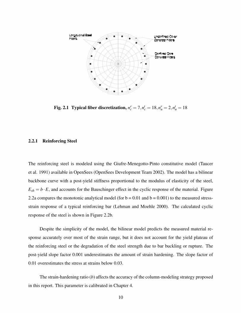
Fig. 2.1 Typical fiber discretization, nrc = 7,nt
c = 18,nru = 2,nt
u = 18
2.2.1 Reinforcing Steel
The reinforcing steel is modeled using the Giufre-Menegotto-Pinto constitutive model (Taucer
et al. 1991) available in OpenSees (OpenSees Development Team 2002). The model has a bilinear
backbone curve with a post-yield stiffness proportional to the modulus of elasticity of the steel,
Esh = b · E, and accounts for the Bauschinger effect in the cyclic response of the material. Figure
2.2a compares the monotonic analytical model (for b = 0.01 and b = 0.001) to the measured stress-
strain response of a typical reinforcing bar (Lehman and Moehle 2000). The calculated cyclic
response of the steel is shown in Figure 2.2b.
Despite the simplicity of the model, the bilinear model predicts the measured material re-
sponse accurately over most of the strain range, but it does not account for the yield plateau of
the reinforcing steel or the degradation of the steel strength due to bar buckling or rupture. The
post-yield slope factor 0.001 underestimates the amount of strain hardening. The slope factor of
0.01 overestimates the stress at strains below 0.03.
The strain-hardening ratio (b) affects the accuracy of the column-modeling strategy proposed
in this report. This parameter is calibrated in Chapter 4.
10

0 0.02 0.04 0.06 0.08 0.10
100
200
300
400
500
600
700
εs
σ (
MP
a)
Measuredb = 0.001b == 0.01
Es*b
Fig. 2.2 Reinforcing steel material model
2.2.2 Concrete
The Popovics curve with model parameters proposed by Mander et al. (1988) was used to model
the responses of both the confined and unconfined concrete in compression. Mander et. al. pro-
posed that the maximum compressive stress of the concrete ( f ′cc) and the strain at the maximum
compressive stress ('cc) should be calculated as follows.
f ′cc = f ′c
(2.254
√
1+7.94fpl
f ′c−2
fpl
f ′c−1.254
)(2.1)
'cc = 0.002(
1+5(
f ′ccf ′c−1
))(2.2)
where:
fpl =12
(sc fytke (2.3)
ke = 1−s′
2dc
1−(lc(2.4)
s′ = s−dtrans (2.5)
(sc = 4(
Ats
dcs
)(2.6)
11

where f ′c is the compressive strength of the concrete, dc is the diameter of the core, and Ats, dtrans,
s and fyt are the area, diameter, spacing and yield stress of the spiral reinforcement. The calculated
stress-strain responses of the confined and unconfined concrete for a typical column are shown in
Figure 2.3.
The concrete was assumed to have strength in tension up to the cracking strength ft . Beyond
this, the strength of the concrete was assumed to decay exponentially to 0.1 ft at 'tu. A detailed
view of the response of the concrete in tension is shown in Figure 2.3b, and the equation governing
the response is as follows.
)(') =
{ Ec' '≤ 't
ft 110
('−'t )('tu−'t ) 't < '≤ 'tu
0.0 ' > 'tu
(2.7)
where 't = ftEc
. This response was developed as part of this project with collaboration with Nilanjan
Mitra.
For the purpose of the development of a cross-section discretization scheme, the concrete was
assumed to crack at a tensile stress of 0.0. For the calibration of the proposed column-modeling
strategies (sections 4 and 6), the concrete was assumed to crack at a tensile stress of ft = 0.625√
f ′c( f ′c in MPa).
−0.03 −0.025 −0.02 −0.015 −0.01 −0.005 0 0.005−1.6
−1.4
−1.2
−1
−0.8
−0.6
−0.4
−0.2
0
0.2
εc
σ/f c,
UnconfinedConfined
(a) Monotonic Response Normalized byCylinder Strength
0 0.5 1 1.50
0.1
0.2
0.3
0.4
0.5
0.6
0.7
0.8
0.9
1
1.1
εc
σ/f t
Ec
εtu
(b) Tensile Response Detail Normalized byTensile Strength
Fig. 2.3 Concrete material models
12
2.3 UNIFORM RADIAL SECTION-DISCRETIZATION STRATEGY
The accuracy and efficiency of moment-curvature analyses depend heavily on the discretization
of the core and cover concrete. A parametric study was performed in order to select the optimal
number of radial and tangential subdivisions of both the confined core concrete (nrc and nt
c) and
unconfined cover concrete (nru and nt
u). In this study, the moment-curvature relationships generated
with the fiber model were compared to the results of a typical moment-curvature analysis program
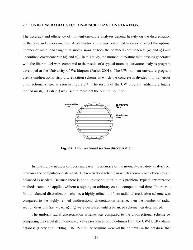
developed at the University of Washington (Parish 2001). The UW moment-curvature program
uses a unidirectional strip discretization scheme in which the concrete is divided into numerous
unidirectional strips, as seen in Figure 2.4. The results of the UW program (utilizing a highly
refined mesh, 100 strips) was used to represent the optimal solution.
Fig. 2.4 Unidirectional section discretization
Increasing the number of fibers increases the accuracy of the moment-curvature analysis but
increases the computational demand. A discretization scheme in which accuracy and efficiency are
balanced is needed. Because there is not a unique solution to this problem, typical optimization
methods cannot be applied without assigning an arbitrary cost to computational time. In order to
find a balanced discretization scheme, a highly refined uniform radial discretization scheme was
compared to the highly refined unidirectional discretization scheme, then the number of radial
section divisions (i.e. nrc, nt
c, nru, nt
u) were decreased until a balanced scheme was determined.
The uniform radial discretization scheme was compared to the unidirectional scheme by
comparing the calculated moment-curvature responses of 75 columns from the UW-PEER column
database (Berry et al. 2004). The 75 circular columns were all the columns in the database that
13

failed in shear or flexure-shear, and had circular spiral reinforcement. This study used a bilinear
steel model (b = 0.01, Section 2.2.1) and the Mander concrete model for both the confined and
unconfined concrete (Section 2.2.2). The moment-curvature response was evaluated based on three
parameters.
!y Ratio, The ratio of curvature at first yielding of the tension steel calculated with the unidirec-
tional scheme to those calculated with the uniform radial scheme, !unidy
!radialy
M5'y Ratio, The ratio of calculated moment at a tensile strain of 5 times 'y calculated with the
unidirectional scheme to the moment calculated with the uniform radial scheme,Munid
5'yMradial
5'y
M10'y Ratio, The ratio of calculated moment at a tensile strain of 20 times 'y calculated with the
unidirectional scheme to the moment calculated with the uniform radial scheme,Munid
20'yMradial
20'y
Based on the results of this analysis, the following recommendations are made in order to
efficiently and accurately model the moment-curvature response of a column cross section using a
uniformly distributed radial discretization scheme,
· 20 core transverse subdivisions, ntc = 20
· 10 core radial subdivisions, nrc = 10
· 20 cover transverse subdivisions, ntu = 20
· 1 cover radial subdivision nru = 1
The mean !y ratio using this scheme is 1.000 with a coefficient of variation (c.o.v.) of
0.110%. The mean M5'y ratio is 0.996 with a coefficient of variation of 0.128% and the mean
M20'y ratio is 0.996 with a coefficient of variation of 0.233%. This configuration is shown in
Figure 2.5.
A parametric study was performed to verify that the recommended discretization scheme ac-
curately and efficiently models moment-curvature response. The parametric study used a bilinear
steel model (b = 0.01) and the Mander concrete model for both the confined and unconfined con-
crete. The recommended scheme was used as the base discretization scheme, and the number of
radial divisions were systematically varied to demonstrate the analyses dependency on the varied
parameter.
14

Recommended Configuration 200 Core Fibers
Fig. 2.5 Recommended configuration, ntc = 20, nr
c = 10, ntu = 20 and nr
u = 1
Figures 2.6 and 2.7 show the effects of varying the number of confined concrete radial and
tangential subdivisions. The mean values of the !y, M5'y , and M10'y ratios are plotted versus nrc in
Figure 2.6 and ntc in Figure 2.7. Also shown in the figures are the maximum and minimum values
and the coefficient of variation of the ratios. Figure 2.6 shows that an unbiased results can be
obtained by using at least 10 radial subdivisions and that using more than 10 does not significantly
improve results. It can be seen in Figure 2.7 that although the mean values vary slightly between
20 and 40 tangential subdivisions, the coefficients of variation of the ratios are the same. Using
more than 20 subdivisions is unnecessary, since the mean value of the ratios using 20 subdivisions
is 0.996 and the coefficient of variation does not improve by using more divisions.
Similarly, the effects of varying the number of unconfined concrete radial and tangential sub-
divisions on moment-curvature accuracy is illustrated in figures 2.8 and 2.9. Figure 2.8 shows that
varying the number of radial unconfined subdivisions does not affect the accuracy of the moment-
curvature analysis significantly. In Figure 2.9, it can be seen that the solutions converge when
ntu = 20 and that using a finer mesh does not significantly improve the accuracy of the moment-
curvature analyses.
15

1 2 4 5 10 15 200.95
1
1.05
ncr
φ y Rat
io
meanmaxmin
1 2 4 5 10 15 200
0.5
1
1.5
2
ncr
CO
V.(%
)
1 2 4 5 10 15 200.95
1
1.05
ncr
Mo
men
t R
atio
at
5 ε y
meanmaxmin
1 2 4 5 10 15 200
0.5
1
1.5
2
ncr
CO
V.(%
)
1 2 4 5 10 15 200.95
1
1.05
ncr
Mo
men
t R
atio
at
20 ε
y
meanmaxmin
1 2 4 5 10 15 200
0.5
1
1.5
2
ncr
CO
V.(%
)
Fig. 2.6 Effect of nrc on m-! accuracy
5 10 15 20 30 400.95
1
1.05
nct
φ y Rat
io
meanmaxmin
5 10 15 20 30 400
0.5
1
1.5
2
nct
CO
V.(%
)
5 10 15 20 30 400.95
1
1.05
nct
Mo
men
t R
atio
at
5 ε y
meanmaxmin
5 10 15 20 30 400
0.5
1
1.5
2
nct
CO
V.(%
)
5 10 15 20 30 400.95
1
1.05
nct
Mo
men
t R
atio
at
20 ε
y
meanmaxmin
5 10 15 20 30 400
0.5
1
1.5
2
nct
CO
V.(%
)
Fig. 2.7 Effect of ntc on m-! accuracy
16

1 2 3 4 5 7 100.95
1
1.05
nur
φ y Rat
io
meanmaxmin
1 2 3 4 5 7 100
0.5
1
1.5
2
nur
CO
V.(%
)
1 2 3 4 5 7 100.95
1
1.05
nur
Mo
men
t R
atio
at
5 ε y
meanmaxmin
1 2 3 4 5 7 100
0.5
1
1.5
2
nur
CO
V.(%
)
1 2 3 4 5 7 100.95
1
1.05
nur
Mo
men
t R
atio
at
20 ε
y
meanmaxmin
1 2 3 4 5 7 100
0.5
1
1.5
2
nur
CO
V.(%
)
Fig. 2.8 Effect of nru on m-! accuracy
5 10 15 20 30 400.95
1
1.05
nut
φ y Rat
io
meanmaxmin
5 10 15 20 30 400
0.5
1
1.5
2
nut
CO
V.(%
)
5 10 15 20 30 400.95
1
1.05
nut
Mo
men
t R
atio
at
5 ε y
meanmaxmin
5 10 15 20 30 400
0.5
1
1.5
2
nut
CO
V.(%
)
5 10 15 20 30 400.95
1
1.05
nut
Mo
men
t R
atio
at
20 ε
y
meanmaxmin
5 10 15 20 30 400
0.5
1
1.5
2
nut
CO
V.(%
)
Fig. 2.9 Effect of ntu on m-! accuracy
17

2.4 NONUNIFORM RADIAL DISCRETIZATION STRATEGY
Because the area nearest the column-neutral axis does not significantly affect moment-curvature
response, it may sometimes be efficient to use a coarser fiber mesh in this region. Utilizing this
scheme would reduce the number of fiber sections required to model the moment-curvature re-
sponse significantly, thus reducing the computational demand of the analysis. It should be noted
that the amount of axial load will affect the location of the neutral axis, and the location will not al-
ways be at the center of the column. The dataset used in the following analysis contained columns
with a wide range of axial-load ratios ( PAg f ′c
= 0 to 70%). In this section the effect of using a coarser
mesh near the center of the cross section is studied and recommendations are proposed for utilizing
this methodology.
A parametric study was performed in which the diameter of a coarse mesh in the center of a
cross section was varied from 50% - 70% of the core diameter (i.e., dcoarsedcore
= 0.5, 0.6 and 0.7) and
the number of coarse mesh fibers (ncoarse) was varied between 10 and 20 fibers. The density of the
fine mesh near the exterior of the core remained the same regardless of the coarse mesh diameter;
therefore an increase in the diameter of coarse mesh resulted in a decrease in the total number
of core fibers (ntotal). The nonuniform configurations were also compared to the recommended
uniform configuration from the previous section (Figure 2.5). Table 2.1 describes the parameter
study matrix and Figure 2.10 illustrates the various configurations. As seen in the table and the
figures, the total number of core fibers was varied from 200 to 70.
The accuracy of the moment-curvature analysis was evaluated using the !y, M5'y and M20'y
ratios as defined in the previous section, and the same 75 columns from the UW-PEER database.
The study used a bilinear steel model (b = 0.01, Section 2.2.1) and the Mander concrete model for
both the confined and unconfined concrete (Section 2.2.2).
As expected, the accuracy of the moment-curvature analysis decreases as the size of the
coarse mesh increases. Decreasing the number of coarse fibers has a similar effect. Utilizing any
of these schemes reduces the number of fibers, but some accuracy is lost. The accuracy lost by
utilizing configuration 1 is within acceptable bounds. With configuration 1, the mean, minimum,
and maximum values of the !y, M5'y , and M20'y ratios are all within 0.01 of 1.00 and the coefficients
of variation are all less than 0.25%. The loss in accuracy from configurations 2-6 are significant
enough to outweigh the resulting gains in efficiency.
18

Table 2.1 Discretization study matrix
Configuration Unif. 1 2 3 4 5 6
dcoarse
dcore0 0.5 0.5 0.6 0.6 0.7 0.7
ntf ine 20 20 20 20 20 20 20
nrf ine 10 5 5 4 4 3 3
ntcoarse 0 10 10 10 10 10 10
nrcoarse 0 2 1 2 1 2 1ntotal 200 120 110 100 90 80 70
2.5 SUMMARY
The constitutive material models used in this report were presented. The reinforcing steel was
modeled using the Giufre-Menegotto-Pinto constitutive model, and the confined and unconfined
concrete was modeled using a model proposed by Mander, Priestley, and Park. The following
parameter was identified for calibration with experimental results.
Strain-Hardening Ratio (b). The ratio of post-yield stiffness of the reinforcing steel to the mod-
ulus of elasticity of the steel, b = EshE .
This parameter is calibrated in Chapter 4. A second parameter was identified, but will not be part
of the optimization study. The effect of the following parameter is studied in 4.6.
Transverse Reinforcement Effectiveness Ratio (*). The ratio of the effective core transverse re-
inforcement ratio to the calculated transverse reinforcement ratio to be used in the calculation
of f ′cc and ecc, * = (e f fsc
(sc.
A parametric study was performed to determine the best uniform radial discretization scheme
to use for modeling column cross-section response. Based on the results of these analyses, the
following recommendations are made in order to efficiently and accurately model the moment-
curvature response of a column cross section using a fiber model: ntc = 20, nr
c = 10, ntu = 20 and
nru = 1. This configuration is shown in Figure 2.5.
Because the area nearest the center of the column influences the column section response
little, a coarser mesh may be used near the center of the column. The effect of using a coarser
19

Configuration 1120 Core Fibers
Configuration 3100 Core Fibers
Configuration 580 Core Fibers
Configuration 2110 Core Fibers
Configuration 490 Core Fibers
Configuration 670 Core Fibers
Fig. 2.10 Configuration types
mesh near the center of the cross section was also studied in this chapter. Since some accuracy is
lost by utilizing this methodology, it is recommended that a uniform discretization with 200 core
fibers (Fig. 2.5) be used when accuracy is the top priority. In cases where efficiency is a concern,
configuration 1 (120 core fibers) could be used also.
20
Unif. 1 2 3 4 5 60.95
1
1.05
Configurations
φ y Rat
io
meanmaxmin
Unif. 1 2 3 4 5 60
0.5
1
1.5
2
Configurations
CO
V.(%
)
Unif. 1 2 3 4 5 60.95
1
1.05
Configurations
Mo
men
t R
atio
at
5εy
meanmaxmin
Unif. 1 2 3 4 5 60
0.5
1
1.5
2
Configurations
CO
V.(%
)
Unif. 1 2 3 4 5 60.95
1
1.05
Configurations
Mo
men
t R
atio
at
20ε y
meanmaxmin
Unif. 1 2 3 4 5 60
0.5
1
1.5
2
Configurations
CO
V.(%
)
Fig. 2.11 Effect of discretization scheme on m−! accuracy
21

3 Development of Distributed-PlasticityColumn Model
In this chapter, a column-modeling strategy is presented, and key modeling parameters are identi-
fied for calibration. In the proposed modeling strategy, a force-based fiber beam-column element,
a zero-length bond section, and an elastic shear component are combined to model the flexural,
bond slip, and shear components of the total column deflection. A graphical interpretation of the
model is shown in Figure 3.1. The following sections describe each of these components in detail.
Fig. 3.1 Distributed-plasticity model with bond slip and shear components
23

3.1 NONLINEAR FORCE-BASED BEAM-COLUMN ELEMENT (FLEXURE)
The flexural component of the column deflection was modeled with a distributed-plasticity, flexibility-
based, fiber beam-column element. A fiber beam-column element is a line element in which the
moment-curvature response at each integration point is determined from the fiber section assigned
to that integration point.
A flexibility-based formulation assumes a moment-distribution along the length of the col-
umn, and the curvatures at each integration point are subsequently estimated for the moment at
that section. The column response is then obtained through weighted integration of the section
responses (Taucer et al. 1991). Because most inelastic behavior occurs near the base of the col-
umn, the element used in this report utilizes the Gauss-Labotto integration scheme, in which the
integration points are placed at the ends of the element, as well as along the column length.
A force-based fiber beam-column element utilizing a Gauss-Labotto integration scheme was
implemented in MATLAB (2005) to evaluate the effects of strain localization (Section 3.1.1) and
to verify the implementation of the force-based beam-column element in OpenSees (OpenSees
Development Team 2002) (Section 3.4). The MATLAB implementation utilized the section dis-
cretization scheme and material constitutive models discussed in sections 2.1 and 2.2, in which
each fiber was assigned a particular stress-strain response.
3.1.1 Concentration of Local Deformations
The force-based formulation is attractive because it can model the spread of plasticity along the
length of the column using only one element and a number of integration points (Np). However,
force-based elements lose objectivity at the local and/or global level depending on the section
hardening behavior (Coleman and Spacone 2001).
For example, figures 3.2 and 3.3 show the calculated force-deformation responses and the
calculated strain distribution along the height of the column for a column with a hardening section
behavior (b = 0.015). The included plot shows the strain distribution at various levels of deforma-
tion. For these figures, pushover analyses were performed on a typical column from the UW-PEER
database (Lehman et. al. 2000, No. 415). One force-based fiber element was used, and the number
of integration points and the strain-hardening ratios were varied systematically. Both the force-
24

deformation envelope (Fig. 3.2) and the average strains (Fig. 3.3) are insensitive to the number of
integration points used in the analysis. The inelastic strains spread up the height of the column as
the deformation is increased.
In contrast, figures 3.4 and 3.5 show the calculated force-deformation responses and the
calculated strain distributions along the height of the column for a column with nearly a plastic
section response (b = 0.001). The force-deformation response (Fig. 3.4) does not vary with the
number of integration points, but the local strains (Fig. 3.5) vary drastically. Inelastic strains
localized at the base of the column and did not spread to any of the other integration points. This
occurs because the column reaches its load carrying capacity when the when the integration point at
the base reaches the yield moment. As the total deflection increases, the base curvature increases
with constant moment, while the other integration points do not see any change in moment or
curvature (Coleman and Spacone 2001). As seen in Figure 3.5, as the number of integration points
increases, the length of the plastic hinge decreases, resulting in larger base curvatures for a given
tip displacement.
Figures 3.6 and 3.7 show similar plots for a column with softening properties (b = − 0.002).
Both the global and local responses are sensitive to the number of integration points used in the
analysis. As in the column with the plastic section response, strains localize at the base of the
column and increasing the number of integration points decreases the length over which these
strains localize. This decrease in length increases the curvature and strains for a given tip deflection.
For the softening section, the increase in strain causes the column force-deformation response to
degrade quickly (Coleman and Spacone 2001).
25

0 1 2 3 4 5 6 7 8 950
100
150
200
250
300
350
Drift Ratio (%)
Fo
rce
(KN
)
Np = 5
Np = 6
Np = 7
Fig. 3.2 Force-deformation envelope with varying np (hardening)
0 0.05 0.10
0.1
0.2
0.3
0.4
0.5
Max Tensile Strain, εs
% o
f C
olu
mn
Hei
gh
t
0 % of Max Displacement
0 0.05 0.10
0.1
0.2
0.3
0.4
0.5
% o
f C
olu
mn
Hei
gh
t
Max Tensile Strain, εs
20 % of Max Displacement
0 0.05 0.10
0.1
0.2
0.3
0.4
0.5
% o
f C
olu
mn
Hei
gh
t
Max Tensile Strain, εs
40 % of Max Displacement
0 0.05 0.10
0.1
0.2
0.3
0.4
0.5
% o
f C
olu
mn
Hei
gh
t
Max Tensile Strain, εs
60 % of Max Displacement
0 0.05 0.10
0.1
0.2
0.3
0.4
0.5
% o
f C
olu
mn
Hei
gh
t
Max Tensile Strain, εs
80 % of Max Displacement
0 0.05 0.10
0.1
0.2
0.3
0.4
0.5
% o
f C
olu
mn
Hei
gh
t
Max Tensile Strain, εs
100 % of Max Displacement
Np = 5
Np = 6
Np = 7
Fig. 3.3 Strain distributions for varying np (hardening)
26

0 1 2 3 4 5 6 7 8 950
100
150
200
250
Drift Ratio (%)
Fo
rce
(KN
)
Np = 5
Np = 6
Np = 7
Fig. 3.4 Force-deformation envelope with varying np (plateau)
0 0.2 0.40
0.1
0.2
0.3
0.4
0.5
Max Tensile Strain, εs
% o
f C
olu
mn
Hei
gh
t
0 % of Max Displacement
0 0.2 0.40
0.1
0.2
0.3
0.4
0.5
% o
f C
olu
mn
Hei
gh
t
Max Tensile Strain, εs
20 % of Max Displacement
0 0.2 0.40
0.1
0.2
0.3
0.4
0.5
% o
f C
olu
mn
Hei
gh
t
Max Tensile Strain, εs
40 % of Max Displacement
0 0.2 0.40
0.1
0.2
0.3
0.4
0.5
% o
f C
olu
mn
Hei
gh
t
Max Tensile Strain, εs
60 % of Max Displacement
0 0.2 0.40
0.1
0.2
0.3
0.4
0.5
% o
f C
olu
mn
Hei
gh
t
Max Tensile Strain, εs
80 % of Max Displacement
0 0.2 0.40
0.1
0.2
0.3
0.4
0.5
% o
f C
olu
mn
Hei
gh
t
Max Tensile Strain, εs
100 % of Max Displacement
Np = 5
Np = 6
Np = 7
Fig. 3.5 Strain distributions for varying np (plateau)
27

0 1 2 3 4 5 6 7 8 950
100
150
200
250
Drift Ratio (%)
Fo
rce
(KN
)N
p = 5
Np = 6
Np = 7
Fig. 3.6 Force-deformation envelope with varying np (softening)
0 0.2 0.40
0.1
0.2
0.3
0.4
0.5
Max Tensile Strain, εs
% o
f C
olu
mn
Hei
gh
t
0 % of Max Displacement
0 0.2 0.40
0.1
0.2
0.3
0.4
0.5
% o
f C
olu
mn
Hei
gh
t
Max Tensile Strain, εs
20 % of Max Displacement
0 0.2 0.40
0.1
0.2
0.3
0.4
0.5
% o
f C
olu
mn
Hei
gh
t
Max Tensile Strain, εs
40 % of Max Displacement
0 0.2 0.40
0.1
0.2
0.3
0.4
0.5
% o
f C
olu
mn
Hei
gh
t
Max Tensile Strain, εs
60 % of Max Displacement
0 0.2 0.40
0.1
0.2
0.3
0.4
0.5
% o
f C
olu
mn
Hei
gh
t
Max Tensile Strain, εs
80 % of Max Displacement
0 0.2 0.40
0.1
0.2
0.3
0.4
0.5
% o
f C
olu
mn
Hei
gh
t
Max Tensile Strain, εs
100 % of Max Displacement
Np = 5
Np = 6
Np = 7
Fig. 3.7 Strain distributions for varying np (softening)
28

For elements with perfectly plastic section behavior, the calculated curvatures and strains are
sensitive to the number of integration points. For elements with softening section behavior, the
local and global responses of the element are sensitive to the number of integration points. Figure
3.8 summarizes these findings. For this figure, pushover analyses were performed on the 8 columns
tested by Lehman and Moehle (2000). One force-based fiber element was used for each column,
and the number of integration points and the strain-hardening ratios were varied systematically. In
this figure, the average values of the following parameters were plotted versus Np.
Moment at "max Ratio. The moment at maximum displacement ("max) for varying Np normalized
by the moment at maximum displacement for Np = 5,
(MNp
"max
M5"max
).
Max Strain at "max Ratio. The maximum tensile steel strain at maximum displacement for vary-
ing Np normalized by the maximum strain at maximum displacement for Np = 5,
('Np
"max
'5"max
).
As seen in Figure 3.8, the global and local responses of the column with the hardening
sections are insensitive to Np if at least four integration points are used. For the column with
the plastic section, the global response is insensitive to Np, but the local response is not. As the
number of integration points is increased, the strain at maximum displacement also increases. For
the column with a softening section, both the global and local responses are sensitive to Np. As Np
is increased, the moments at maximum displacement decrease and the strains increase.
Similarly, Figure 3.9 illustrates the effect of Np on columns under double curvature for the
three section behaviors. In this figure, the maximum moments and strains are normalized by the
results at 6 Np. As seen in the figure, at least 6 integration points are needed for unbiased global
and local results for columns with hardening sections under double curvature.
29

3 4 5 6 7 80
0.5
1
1.5
2
2.5
3
Np
Mea
n S
trai
n a
t ∆
max
Rat
io
3 4 5 6 7 80.7
0.8
0.9
1
1.1
Np
Mea
n M
om
ent
at ∆
max
Rat
io b = 0.015b = 0.001b = −0.002
b = 0.015b = 0.001b = −0.002
Fig. 3.8 Force-deformation and strain dependency on np (cantilever)
30

3 4 5 6 7 80
0.5
1
1.5
2
2.5
3
Np
Mea
n S
trai
n a
t ∆
max
Rat
io
3 4 5 6 7 80.7
0.8
0.9
1
1.1
Np
Mea
n M
om
ent
at ∆
max
Rat
io b = 0.015b = 0.001b = −0.002
b = 0.015b = 0.001b = −0.002
Fig. 3.9 Force-deformation and strain dependency on np (double curvature)
31

The issue of the concentration of local deformations in distributed-plasticity elements was
addressed by Coleman and Spacone (2001). The researchers developed a method of post-processing
plastic curvatures to obtain nonbiased curvatures based on assumed plastic-hinge lengths (Lp).
The post-processing method was developed by equating equations for tip displacements from tra-
ditional plastic-hinge analysis (+lumpedp ) to the tip displacements calculated from the distributed-
plasticity element (+distributedp ), and then adjusting the distributed-plasticity plastic curvatures to
match the curvatures from the lumped-plasticity formulation. This process is described in more
detail in the following discussion.
The plastic tip displacement for a cantilever column calculated from traditional plastic-hinge
analysis is as follows.
+lumpedp = !pLp
(L−
Lp
2
)(3.1)
where !p is the plastic curvature in the hinge, and L is the column length. The plastic-displacement
for a cantilever column calculated with the distributed-plasticity element can be simplified to the
following equation.
+distributedp = !p1Lip1
(L−
Lip1
2
)+!p2Lip2
(L−Lip1−
Lip2
2
)+ ... (3.2)
where !p1 and !p2 are the plastic curvatures calculated at the first and second integration points in
the element. Lip1 and Lip2 are the equivalent plastic-hinge lengths of the first and second integration
points. In this formulation, the plastic-hinge lengths for the integration points are calculated as
Lip1 = wip1L and Lip2 = wip2L. wip1 and wip2 are the weights of the respective integration points
according to the integration scheme. The traditional implementation of the force-based element
uses Gauss-Labotto integration.
Equation 3.2 can be carried out to include the other integration points; however the plastic
deformations rarely spread to the other integration points. In fact, in the case of a softening section
response, the plastic deformations will not spread to the second integration point, and will be
concentration in the first integration point at the base of the column, as illustrated in Figure 3.7.
The post-processing method developed by Coleman and Spacone (2001) was formulated for
a softening section, and therefore the second integration point terms in Equation 3.2 are ignored. By
equating the first integration point terms of Equation 3.2 to Equation 3.1, the following relationship
32

is obtained for the nonbiased, adjusted plastic curvature (!ad j1p ) as a function of the weight of the
integration point, plastic-hinge length, and calculated curvature.
!ad j1p = !p1
wip1L2 (2−wip1)Lp (2L−Lp)
(3.3)
This formulation is correct for softening sections; however if there is any hardening in the section,
and plastic deformations spread to the second integration point, it will no longer be valid. In the
case of a hardening section, the calculated curvatures from the distributed-plasticity element will
be nonbiased, but will not match the curvatures calculated with the traditional lumped-plasticity
formulation.
A similar relationship for the nonbiased adjusted plastic curvature can be obtained for hard-
ening sections by including the higher integration points. The following relationship is obtained
by including the second integration point in 3.2.
!ad j2p = !p1
wip1L2 (2−wip1)Lp (2L−Lp)
+!p2wip2L2 (2−2wip1−wip2)
Lp (2L−Lp)(3.4)
This relationship will be valid as long as plastic deformations do not spread to the third integration
point. The following figures (figures 3.10-3.12) demonstrate the concepts discussed above.
In Figure 3.10 the post-yield strain-hardening ratio (b) of the steel in the distributed-plasticity
element is varied between -1.0 % and 5.0% for a typical column in the database using 5 integration
points and neglecting bar slip and shear deformations. The first axes in this figure illustrates the
recorded curvatures at the first integration point. The second axes is a plot of the adjusted plastic
curvatures calculated with one integration point (Equation 3.3) versus displacement ductility. The
third axes is a plot of the adjusted-plastic curvature calculated with two integration points (Equa-
tion 3.4) versus displacement ductility. The fourth axes is a plot of the ratio of plastic curvature
calculated at the second integration point to the curvatures at the first integration point. This axes is
included to demonstrate the amount of plastic deformation that has spread to the second integration
point.
As seen in the figure, the recorded curvature at the first integration point is dependent on
the amount of hardening or softening in the column, and the curvatures do not match the curva-
tures calculated with plastic-hinge analysis. In the case of the softening section response, utilizing
33

one integration point in the calculation of the adjusted plastic curvature is sufficient, however the
method is inaccurate for the hardening section responses, as expected. As seen in the third axes,
the adjusted curvatures using two integration points match the target curvatures of the lumped-
plasticity formulation for both the hardening and softening section responses.
Similarly, in Figure 3.11 the number of integration points is varied between 5 and 8 for
a typical column in the database with a softening section response (b = −1.00%). As seen in
the first axes, the curvatures recorded at the base of the column are dependent on the number of
integration points used in the calculation. As shown in the second and third axes, both nonbiased
curvatures calculated with both methods are identical to the target curvatures from the lumped-
plasticity formulation.
In Figure 3.12, the number of integration points is varied between 5 and 8 for a typical col-
umn in the database with a hardening section response (b = 5.00%). As seen in the first axes, the
curvatures at the base of the column are not dependent on the number of integration points used in
the calculation; however, these curvatures do not match those calculated with the lumped-plasticity
formulation. The second axes illustrates the inability of Equation 3.3 to calculated unbiased curva-
tures for hardening sections. The third axes demonstrates that Equation 3.4 is accurate (in particu-
lar case) for 5, 6, and 7 integration points, but begins to stray at higher ductilities for 8 integration
points. This is because the plastic curvatures begin to spread to the third integration point.
34
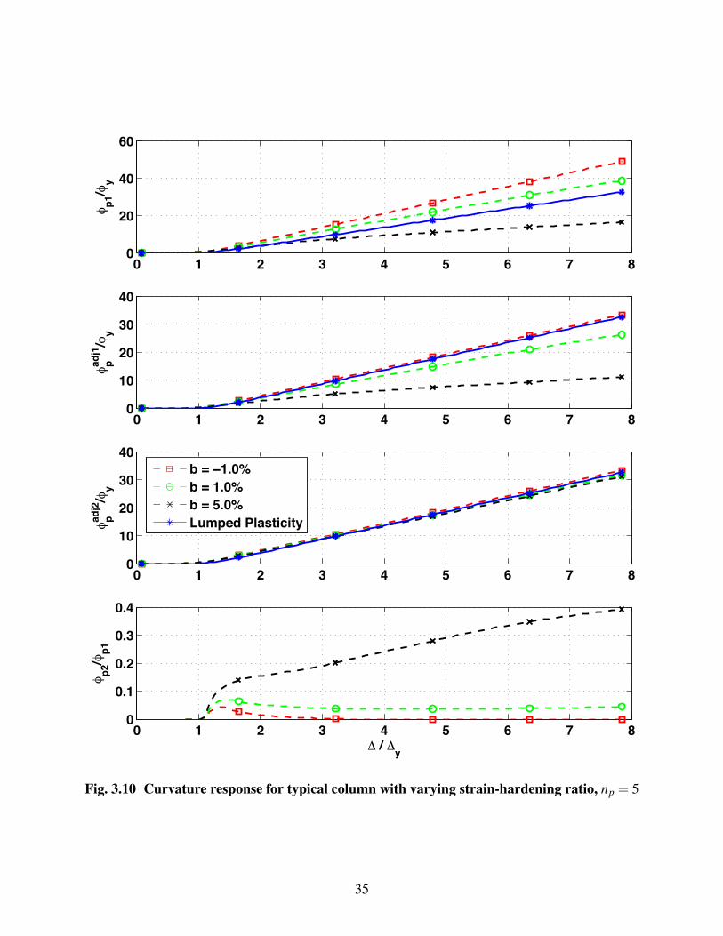
0 1 2 3 4 5 6 7 80
20
40
60
φ p1/φ
y
0 1 2 3 4 5 6 7 80
10
20
30
40
φ padj1
/φy
0 1 2 3 4 5 6 7 80
10
20
30
40
φ padj2
/φy
0 1 2 3 4 5 6 7 80
0.1
0.2
0.3
0.4
∆ / ∆y
φ p2/φ
p1
b = −1.0%b = 1.0%b = 5.0%Lumped Plasticity
Fig. 3.10 Curvature response for typical column with varying strain-hardening ratio, np = 5
35

0 1 2 3 4 5 6 7 80
50
100
150
φ p1/φ
y
0 1 2 3 4 5 6 7 80
10
20
30
40
φ padj1
/φy
0 1 2 3 4 5 6 7 80
10
20
30
40
φ padj2
/φy
0 1 2 3 4 5 6 7 80
0.2
0.4
0.6
0.8
∆ / ∆y
φ p2/φ
p1
Np = 5
Np = 6
Np = 7
Np = 8
Lumped Plasticity
Fig. 3.11 Curvature response for typical column with degrading section response,b =−1.00%
36

0 1 2 3 4 5 6 7 80
10
20
30
φ p1/φ
y
0 1 2 3 4 5 6 7 80
10
20
30
φ padj1
/φy
0 1 2 3 4 5 6 7 80
10
20
30
40
φ padj2
/φy
0 1 2 3 4 5 6 7 80
0.2
0.4
0.6
0.8
∆ / ∆y
φ p2/φ
p1
Np = 5
Np = 6
Np = 7
Np = 8
Lumped Plasticity
Fig. 3.12 Curvature response for typical column with hardening section response, b = 5.00%
37

3.2 BOND SLIP DISPLACEMENT MODEL
The fiber-based beam-column element is based on the assumption that plane sections remain plane,
which implies perfect bond between the longitudinal reinforcement and the surrounding concrete
(Hachem et al. 2003). The force-based beam-column element does not include the component of
deformation due to bond slip, and the column appears stiffer than it actually is. In the proposed
modeling strategy, a zero-length section at the base of the column is used to model the bond slip
of the anchorage reinforcement. The zero-length section is a fiber section in which each fiber is
assigned a stress-displacement relationship instead of a stress-strain relationship. This formulation
is beneficial because it allows for biaxial, cyclic lateral loading and variable axial loads.
3.2.1 Tensile Stress-Displacement Relationship of Reinforcement
The steel stress-displacement relationship was based on a two-component bond-stress model
(Lehman and Moehle 2000). The model was modified by Ranf (2006) to account for development
of bond stress at low bar strains. An illustration of the model is presented in Fig. 3.13. In this
τ(σ)
σ
τe(σ)
τi(σ)
τd(σ)
σ σd y
Fig. 3.13 Bond model illustration
figure, ) is the axial stress in the longitudinal reinforcement, &i()) is the bond stress above the
yield stress of the reinforcement )y, &e()) is the bond stress above the bar stress that is needed to
fully develop the bond ()d) but below the yield stress. &d()) is the bond stress for stress in the
reinforcement below the development stress. For this model, the elastic and inelastic bond stresses
were assumed to be constant with stress, while the development bond stress was assumed to be
38

linearly related to the stress in the reinforcement. The components of the model are described in
Equation 3.5,
&()) =
{ &e))d
= a))d
√f ′c )≤ )d
&e = #e√
f ′c )d ≤ )≤ )y
&i = #i√
f ′c )y ≤ )
(3.5)
where #e and #i are the elastic and inelastic bond-stress coefficients respectively. Using the bond
stress defined in Eq. 3.5, the change in strain (change in stress) along the length of the reinforce-
ment is described by the differential equation, Equation. 3.6.
dFdx
=,d2
b4
d)dx
= &()),db
d)dx
=4&())
db
(3.6)
By integrating the strains along the development length, the tensile stress-displacement en-
velope of an anchorage bar can be calculated for a column. The stress-displacement envelope for a
typical column is shown in Figure 3.14. For this study, the nonlinear stress-displacement relation-
ships calculated with this method were simplified by assuming a linear relationship from ) = 0 to
) = fy and a second linear relationship between fy and fu as seen in the figure.
0 5 10 15 200
0.5
1
1.5
∆ (mm)
σ /
f y
Lehman ModelSimplified Model
Fig. 3.14 Stress-displacement envelope for typical anchor bar
39

The three parameters of the bond model ()d , #e, and #i) are calibrated by comparing the
strains measured in the columns at the anchorage-column interface with the strains measured 8
inches within the anchorage in Section 4.3.
3.2.2 Compressive Stress-Displacement Relationships
The compressive stress-displacement relationship of the concrete was calculated from the stress-
strain relationship by assuming an effective depth over which the compressive strains act (dcomp),
and multiplying the strains by this assumed depth to obtain a displacement. The assumed depth is
illustrated in Figure 4.11.
Fig. 3.15 Assumed compressive depth
3.2.3 Calibration Parameters
Because of the complexity of bond slip, the proposed bond slip model needs to be calibrated with
experimental results. The key model parameters that need to be calibrated are the bond-strength
ratios #e and #i, and the depth of the compressive strains dcomp. These parameters are calibrated in
Chapter 4.
3.3 SHEAR-DISPLACEMENT MODEL
The shear component ("v) of the total deflection of the column was modeled in accordance with
elastic theory:
"v =k ·V · LG · AG
(3.7)
40

where k is a shape factor to account for the shape of the cross section (k = 43 for circular sections),
V is the transverse shear force, and AG is the gross cross-sectional area. G is the modulus of rigidity
of the concrete and can be estimated as the concrete modulus of elasticity multiplied by a scalar,
G = $Ec, where Ec can be calculated as Ec = 4730√
f ′c, (ACI 318 2002). Park and Paulay (1975)
recommend a value of $ = 0.4 (MPa).
3.4 OPENSEES IMPLEMENTATION
The MATLAB implementation of the force-based beam-column element was developed for mono-
tonic loading. Since both the monotonic and cyclic behavior of a column are important in seis-
mic regions, OpenSees (which is capable of modeling cyclic loading) was used to implement the
proposed distributed-plasticity modeling strategy for the remainder of this report. This section dis-
cusses the implementation of the three major components of column deformation into OpenSees.
3.4.1 Flexural Component
The force-based beam-column element in OpenSees was implemented using the nonlinearBeam-
Column command. The OpenSees implementation was verified by comparing the calculated force-
deformation responses from OpenSees with the calculated force-deformation responses from the
MATLAB implementation for 8 columns (Lehman and Moehle 2000) (Figure 3.16). As seen in
the figure, the force-deformation envelopes calculated with OpenSees are indistinguishable with
the force-deformation envelopes calculated with the stand-alone MATLAB implementation.
3.4.2 Bond Slip Deformation
The bond slip deformation model described in Section 3.2 was implemented in OpenSees using a
zero-length section (zeroLengthSection) placed at the base of the column. The zero-length section
consisted of a fiber section (Section 2.1) in which the stress-deformation response of the steel was
determined in accordance with Section 3.2.1, and the compressive stress-displacement response of
the concrete was determined in accordance with Section 3.2.2. The stress-displacement response
of the steel was modeled with steel02 material model in OpenSees, and the stress-displacement
response of the concrete was modeled with concrete04.
41

3.4.3 Shear Deformation
The shear-deformation model was implemented in OpenSees by aggregating lateral
force-deformation sections into the fiber sections of the beam-column element, as seen in Figure
3.1. The properties of the lateral force-deformation response were determined in accordance with
elastic theory, as described in Section 3.3.
3.4.4 Calculation of Average Strains
The calculated average tensile strain values at two levels of column height are used in the calibra-
tion of the proposed modeling strategy (Section 4.4). Specifically, the measured and calculated
average tensile steel strains are compared from the base of the column to a quarter of the column
depth (0-D/4) and a quarter of the column depth to the total column depth (D/4-D/2). In a fiber
beam-column element, the stresses and strains of any fiber in a section can be recorded. However,
the sections are only located at integration points, and the location of the integration points are
determined from the Gauss-Labotto integration scheme. In order to obtain the average strains from
0-D/4 and D/4-D/2, zero-weight integration points were added to the elements at D/4 and D/2. The
added integration points do not affect the results of the analyses, but provide a means of recording
section and fiber behavior at their locations. The average flexural tensile steel strain values from
0-D/4 were obtained by averaging the strain values recorded at the base of the column and at D/4.
The average strain values were obtained for the D/4-D/2 segment in a similar manner.
The measured average strains from 0-D/4 also include the strains associated with bond slip of
the anchorage reinforcement. In order to compare these strain values with calculated strain values,
a calculated bond slip component was included in the calculated strains. The calculated vertical
displacement of the anchorage steel was recorded from the zero-length bond slip section (Section
3.2). This vertical displacement was then divided by the length D/4 to obtain an average strain, and
then added onto the calculated flexural steel strain.
3.5 SUMMARY
In the proposed modeling strategy, a nonlinear force-based fiber beam-column element, a zero-
length bond section, and an aggregated elastic shear section are combined to model the flexural,
42

bond slip, and shear components of the total tip deflection of a column. The following key model-
ing parameters were identified:
Number of Integration Points (Np). The number of integration points used in the flexibility-based,
fiber beam- column element.
Bond-Strength Ratios (#e and #i). The ratio of bond strength to the square root of the compres-
sive strength of the concrete, #e = &be√f ′c
and #i = &bi√f ′c
.
Development Bar Stress ()d). The bar stress required to fully develop the bond.
Bond-Model Compression Depth (dcomp). The effective depth of the compression strains for the
concrete in the zero-length bond-slip element.
Shear-Stiffness Ratio ($). The ratio of the modulus of rigidity of the concrete to the modulus of
elasticity of the concrete, $ = GEc
.
43

0 0.5 1 1.5 2 2.5 3 3.5 40
50
100
150
200
250
300
Drift (%)
Fo
rce
(KN
)
Lehman No.415
OpenSeesStand Alone
0 1 2 3 4 5 6 70
50
100
150
Drift (%)
Fo
rce
(KN
)
Lehman No.815
OpenSeesStand Alone
0 1 2 3 4 5 6 7 80
20
40
60
80
100
120
Drift (%)
Fo
rce
(KN
)
Lehman No.1015
OpenSeesStand Alone
0 0.5 1 1.5 2 2.5 320
40
60
80
100
120
140
160
180
Drift (%)
Fo
rce
(KN
)
Lehman No.407
OpenSeesStand Alone
0 0.5 1 1.5 2 2.5 3 3.5 40
100
200
300
400
500
Drift (%)
Fo
rce
(KN
)
Lehman No.430
OpenSeesStand Alone
0 0.5 1 1.5 2 2.5 30
100
200
300
400
500
600
Drift (%)
Fo
rce
(KN
)
Lehman & Calderone No.328
OpenSeesStand Alone
0 1 2 3 4 5 6 70
50
100
150
200
250
Drift (%)
Fo
rce
(KN
)
Lehman & Calderone No.828
OpenSeesStand Alone
0 2 4 6 8 100
50
100
150
200
Drift (%)
Fo
rce
(KN
)
Lehman & Calderone No.1028
OpenSeesStand Alone
Fig. 3.16 Comparison of calculated f-" envelopes
44
4 Calibration of Distributed-PlasticityColumn Model
To accurately model reinforced concrete column behavior, the distributed-plasticity modeling strat-
egy proposed in Chapter 3 was calibrated with experimental results. The modeling parameters
identified for calibration in chapters 2 and 3 are:
Strain-Hardening Ratio (b). The ratio of post-yield stiffness of the reinforcing steel to the mod-
ulus of elasticity of the steel, b = EshE (Section 2.2.1).
Bond-Strength Ratios (#e and #i). The ratio of bond strength to the square root of the compres-
sive strength of the concrete, #e = &be√f ′c
and #i = &bi√f ′c
.
Development Bar Stress ()d). The bar stress required to fully develop the bond.
Number of Integration Points (Np). The number of integration points used in the flexibility-based,
fiber beam-column element (Section 3.1).
Bond-Model Compression Depth (dcomp). The effective depth of the compression strains for the
concrete in the zero-length bond-slip element (Section 3.2).
Shear-Stiffness Ratio ($). The ratio of the modulus of rigidity of the concrete to the modulus of
elasticity of the concrete, $ = GEc
(Section 3.3).
This chapter discusses the calibration strategy used in this report and presents the results
of this analysis. The results of a sensitivity analysis are then presented to identify the effects of
varying key parameters.
45

4.1 COLUMN DATA
A subset of eight columns from the bridge column dataset designated in Section 1.3 was used to
calibrate the distributed-plasticity column-modeling strategy. The eight columns were the experi-
ments documented in Lehman and Moehle (2000), and are included in Table 1.1. These columns
were selected because they met Caltrans/AASHTO detailing requirements and the following data
were available.
· Force-displacement histories
· Strain-gage histories
· Relative-rotation histories (average curvature)
· Observations of damage
This data were not available for all columns in the database, specifically the strain-gage data and
average rotations.
Because estimating both global and local deformations are important, the force-displacement
envelopes and the average strains in the tensile reinforcement were used in the calibration of the
distributed-plasticity model. The force-displacement envelopes and average strain-displacement
envelopes were extracted from the recorded digital force-displacement histories of the column with
the algorithm described in Parish (2001). The average strains were calculated from the average
rotations measured with the potentiometers as described in Appendix C of Lehman and Moehle
(2000).
The average strains at two different levels of the column height were used in the calibration
of the distributed-plasticity model, the average strains from the base of the column to one quarter
of the column depth, 0−D/4, and the strains from one quarter of the column depth to half the
column depth, D/4−D/2. It should be noted that the average strains at the base of the column
include deformations from bar slip since the potentiometers at the base of the column measure both
the flexural displacement and the displacement due to bond slip of the anchorage reinforcement.
The average strains were used in this study instead of the strain gages, because potentiome-
ters are able to accurately measure deformation at higher levels of deformation. The average strain
measurements were verified with the strain gages attached to the reinforcement, and at low levels
of deformation, the measurements were similar.
46

4.2 STEEL STRAIN-HARDENING RATIO CALIBRATION
The strain-hardening ratio was calibrated by minimizing the square root of the sum of the squares
of the difference between the calculated response of the steel under monotonic loading to the
measured response from coupon tests up to a strain of 0.1. The measured stress-strain response
used for this calibration was the average response of the coupon tests performed by Lehman and
Moehle (2000). A value of b = 0.0097 minimized the normalized error with a value of 3.91%.
However, for simplicity, b = 0.01 was selected as the optimal value, (normalized error = 3.93%).
The measured and calculated material responses are shown in Figure 4.1.
Fig. 4.1 Measured and calculated stress-strain response of steel
4.3 BOND-STRENGTH MODEL CALIBRATION
Three parameters of the bond model ()d , #e, and #i, defined in Figure 3.13) were calibrated by
comparing the strains measured in the column tests at the anchorage-column interface with the
strains measured six inches within the anchorage. Of the 16 possible strain-gage sets (north and
south locations for the 8 columns), measurements from both of the strain gages were reliable up
to an interface strain of 0.015 for 8 sets. The envelopes of the interface gage strains versus the
anchorage gage strains for the 8 strain-gage sets are shown in Figure 4.2.
The best fit of the envelopes from the 8 strain-gage sets shown in Figure 4.2 was realized
using elastic and inelastic bond-stress coefficients of #e = 0.9 and #i = 0.45, and a development
47

stress of )d = 0.25)y. These values would vary if the steel were modified from the bilinear ap-
proximation, b = 0.01.
0 1 2 3 4 50
0.5
1
1.5
2
ε0
ε −D
/3 (
x 10
−3)
MeasuredCalculated
Fig. 4.2 Bond-strength calibration
4.4 OPTIMIZATION STRATEGY FOR REMAINING MODEL PARAMETERS
4.4.1 Measures of Accuracy
In order to successfully predict the response of a column under seismic loading (including damage
prediction) both the global force-deformation response, and the local curvatures and strains must
be predicted accurately. The calibration of the proposed modeling strategy considered the accuracy
of both the global and local responses. The parameters used in this chapter to measure the accuracy
of the modeling strategy are as follows.
Pushover Error (Epush). The accuracy of the force-displacement envelope was accounted for with
the pushover error, which is defined as
Epush =
√√√√-ni=1
(Fi
meas−Ficalc
)2
(max(Fmeas))2 n(4.1)
48
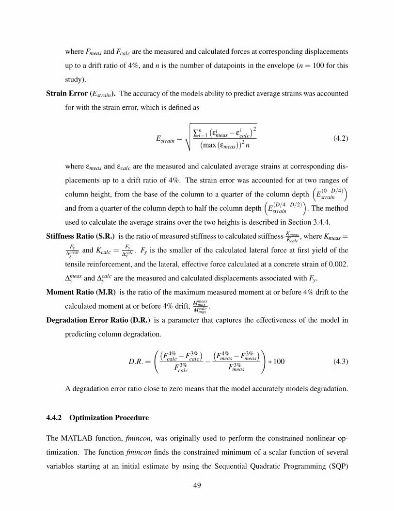
where Fmeas and Fcalc are the measured and calculated forces at corresponding displacements
up to a drift ratio of 4%, and n is the number of datapoints in the envelope (n = 100 for this
study).
Strain Error (Estrain). The accuracy of the models ability to predict average strains was accounted
for with the strain error, which is defined as
Estrain =
√√√√-ni=1
('i
meas− 'icalc
)2
(max('meas))2 n(4.2)
where 'meas and 'calc are the measured and calculated average strains at corresponding dis-
placements up to a drift ratio of 4%. The strain error was accounted for at two ranges of
column height, from the base of the column to a quarter of the column depth(
E(0−D/4)strain
)
and from a quarter of the column depth to half the column depth(
E(D/4−D/2)strain
). The method
used to calculate the average strains over the two heights is described in Section 3.4.4.
Stiffness Ratio (S.R.) is the ratio of measured stiffness to calculated stiffness KmeasKcalc
, where Kmeas =Fy
"measy
and Kcalc = Fy"calc
y. Fy is the smaller of the calculated lateral force at first yield of the
tensile reinforcement, and the lateral, effective force calculated at a concrete strain of 0.002.
"measy and "calc
y are the measured and calculated displacements associated with Fy.
Moment Ratio (M.R) is the ratio of the maximum measured moment at or before 4% drift to the
calculated moment at or before 4% drift, Mmeasmax
Mcalcmax
.
Degradation Error Ratio (D.R.) is a parameter that captures the effectiveness of the model in
predicting column degradation.
D.R. =
((F4%
calc−F3%calc
)
F3%calc
−(F4%
meas−F3%meas
)
F3%meas
)∗100 (4.3)
A degradation error ratio close to zero means that the model accurately models degradation.
4.4.2 Optimization Procedure
The MATLAB function, fmincon, was originally used to perform the constrained nonlinear op-
timization. The function fmincon finds the constrained minimum of a scalar function of several
variables starting at an initial estimate by using the Sequential Quadratic Programming (SQP)
49

method (MATLAB 2000). However, this method was abandoned because the presence of multiple
local minimums hindered the methods ability to obtain the global minimum.
The optimization was performed by running a pushover analysis for a broad range of mod-
eling parameters and then selecting the scheme in which the mean total error (Etotal , Equation 4.4)
was minimized and the additional modeling accuracy terms (e.g., stiffness ratio) were reasonable.
The range of values used for each calibration parameter are shown in Table 4.1, along with the step
size between consecutive values within the range. The analysis consisted of every combination of
the optimization parameters. Where c is equal to the column’s neutral axis depth at a maximum
Table 4.1 Calibration parameter ranges for initial run
parameter Np dcomp $
min 4 0.1 c 0.10max 7 2.0 c 0.80
step size 1 0.1 c 0.10
compressive strain of 0.002 (c). In addition to the parameter values indicated in the table, the model
without shear deformation was also considered in the optimization (i.e., $ = .).
The objective function for the optimization was a combination of the average pushover error
and average strain errors at the two ranges of the column height. The total error, Etotal , is defined
as
Etotal =12
mean(Epush
)+
/1
4mean
(E(0−D/4)
strain
)+
%2
4mean
(E(D/4−D/2)
strain
)(4.4)
where:
/1 =min
(mean
(Epush
))
min(
mean(
E(0−D/4)strain
)) (4.5)
/2 =min
(mean
(Epush
))
min(
mean(
E(D/4−D/2)strain
)) (4.6)
where mean entails the average value over the eight Lehman and Moehle (2000) columns, and min
entails the minimum value out of the total number of combinations. The % terms are included to
ensure that the error terms are of similar magnitude.
50

4.5 OPTIMIZATION RESULTS
The optimization study described in the previous section was performed for the eight columns
described by Lehman and Moehle (2000). The top 20 combinations from the optimization study
are reported in Table 4.2. The accuracy measures reported in this table (e.g., Etotal and S.R.) are
average values for the eight columns.
Table 4.2 Distributed-plasticity optimization results
Parameter Values Measures of Accuracy
Rank N p dcomp $ Etotal Epush E0−D/4strain ED/4−D/2
strain S.R. M.R. D.R1 6 0.8 c 0.1 7.02 6.62 6.83 16.94 0.91 1.03 0.872 6 0.7 c 0.1 7.02 6.60 6.95 16.77 0.90 1.03 0.863 6 1 c 0.1 7.03 6.63 6.78 17.07 0.92 1.03 0.924 6 0.9 c 0.1 7.04 6.63 6.82 17.06 0.91 1.03 0.905 6 1.1 c 0.1 7.05 6.65 6.70 17.32 0.92 1.04 0.946 6 1.2 c 0.1 7.05 6.65 6.59 17.58 0.93 1.04 0.937 6 0.6 c 0.1 7.06 6.62 7.15 16.51 0.89 1.03 0.788 6 1.3 c 0.1 7.07 6.67 6.50 17.87 0.93 1.04 1.029 6 1.4 c 0.1 7.07 6.67 6.47 17.98 0.94 1.04 1.06
10 6 1.6 c 0.1 7.08 6.69 6.43 18.08 0.94 1.04 1.1011 6 1.5 c 0.1 7.08 6.68 6.45 18.07 0.94 1.04 1.1112 6 0.9 c 0.2 7.11 6.72 6.97 16.94 0.89 1.03 0.9113 6 0.9 c 0.3 7.11 6.72 6.97 16.94 0.89 1.03 0.9114 6 0.9 c 0.5 7.11 6.72 6.97 16.94 0.89 1.03 0.9115 6 0.9 c 0.6 7.11 6.72 6.97 16.94 0.89 1.03 0.9116 6 0.9 c 0.7 7.11 6.72 6.97 16.94 0.89 1.03 0.9117 6 1.7 c 0.1 7.11 6.70 6.43 18.33 0.95 1.04 1.1218 6 1.1 c 0.2 7.12 6.75 6.80 17.29 0.90 1.03 0.9419 6 1.1 c 0.3 7.12 6.75 6.80 17.29 0.90 1.03 0.9420 6 1.1 c 0.5 7.12 6.75 6.80 17.29 0.90 1.03 0.94
It was difficult to objectively select an optimal solution from this analysis because many
combinations of parameters resulted in nearly identical values of Etotal . The proposed modeling
strategy was not sensitive to several of the optimization parameters, and the optimization results
were dominated by several combinations that differed only by those parameters. For example, the
only parameter that differs between the top 11 ranked combinations is the bond penetration depth
(dcomp).
The effect of Np on the optimization surface can be observed by sorting the optimization
results first by Np and then by Etotal , and then plotting the normalized error(
EtotalEmin
total−1
)versus
the normalized rank order (i.e., the ranking divided by the total number of combinations) (Figure
4.3). The normalized error varied from 0 (Etotal = 7.02) to 0.92 (Etotal = 13.46). As seen in the
figure, the best results are obtained for Np = 6. Nonetheless, as long as five integration points are
used, similar minimum values of Etotal can be obtained. This result can be explained by noting
51

0
0.1
0.2
0.3
0.4
0.5
0.6
0.7
0.8
0.9
1
0 0.1 0.2 0.3 0.4 0.5 0.6 0.7 0.8 0.9 1
Relative Rank Order
No
rma
lize
d E
rro
r
Np = 4 Np = 5 Np = 6 Np = 7
Fig. 4.3 Effect of np on optimization surface
that the columns being studied are well-confined columns with hardening section behavior. For
such sections the number of integration points should not significantly affect the calculated global
or local responses (Section 3.1.1). For modeling efficiency, the combinations with five integration
points will be used to select the optimal solution.
Table 4.3 provides the top 20 combinations in which Np = 5. As seen in the table, the
combination that minimizes the total error (Etotal = 7.13) is dcomp = 0.4c and $ = 0.1. As seen in
Table 4.3, $ does not significantly affect the accuracy of the model. The combination with $ = 0.4
(# 16, dcomp = 0.5c, Etotal = 7.21) will be chosen as the optimal solution to remain consistent with
previous research Park and Paulay (1975).
52

Table 4.3 Distributed-plasticity optimization results (np = 5, $ = 0.4 and dcomp = c)
Parameter Values Measures of Accuracy
Rank N p dcomp $ Etotal Epush E0−D/4strain ED/4−D/2
strain S.R. M.R. D.R1 5 0.4 c 0.1 7.13 6.85 6.57 17.52 0.87 1.04 0.352 5 0.5 c 0.1 7.15 6.83 6.52 17.87 0.88 1.04 0.423 5 0.3 c 0.1 7.16 6.91 6.78 17.02 0.86 1.04 0.314 5 0.6 c 0.1 7.17 6.82 6.49 18.22 0.89 1.04 0.445 5 0.4 c 0.2 7.19 6.96 6.62 17.37 0.85 1.04 0.366 5 0.4 c 0.3 7.19 6.96 6.62 17.37 0.85 1.04 0.367 5 0.4 c 0.5 7.19 6.96 6.62 17.37 0.85 1.04 0.368 5 0.4 c 0.6 7.19 6.96 6.62 17.37 0.85 1.04 0.369 5 0.4 c 0.7 7.19 6.96 6.62 17.37 0.85 1.04 0.36
10 5 0.5 c 0.2 7.20 6.96 6.52 17.73 0.86 1.04 0.4011 5 0.5 c 0.3 7.20 6.96 6.52 17.73 0.86 1.04 0.4012 5 0.5 c 0.5 7.20 6.96 6.52 17.73 0.86 1.04 0.4013 5 0.5 c 0.6 7.20 6.96 6.52 17.73 0.86 1.04 0.4014 5 0.5 c 0.7 7.20 6.96 6.52 17.73 0.86 1.04 0.4015 5 0.7 c 0.1 7.20 6.84 6.46 18.47 0.90 1.04 0.4816 5 0.5 c 0.4 7.21 7.02 6.51 17.61 0.85 1.04 0.3817 5 0.6 c 0.2 7.21 6.94 6.44 18.14 0.87 1.04 0.4318 5 0.6 c 0.3 7.21 6.94 6.44 18.14 0.87 1.04 0.4319 5 0.6 c 0.5 7.21 6.94 6.44 18.14 0.87 1.04 0.4320 5 0.6 c 0.6 7.21 6.94 6.44 18.14 0.87 1.04 0.43
The selected optimal solution is as follows.
Strain-Hardening Ratio, b = 0.01.
Bond-Strength Ratios, #e = 0.9 and #i = 0.45.
Development Bar Stress, )d = 0.25)y .
Number of Integration Points, Np = 5.
Bond-Model Compression Depth, dcomp = 0.5c (Half the N.A. Depth at 'c = 0.002).
Shear-Stiffness Ratio, $ = 0.4.
This combination of parameters resulted in the following mean measures of accuracy: Etotal =
7.22, Epush = 7.02, E(0−D/4)strain = 6.51, E(D/4−D/2)
strain = 17.73, stiffness ratio = 0.85, moment ratio =
1.04 and degradation error ratio = 0.38. The corresponding coefficients of variation (%) for these
measures were 20, 43, 44, 44, 11, 8, and -.
In a pilot study, a similar optimization was run without including the tensile strength of the
concrete, and using the bond-strength ratios proposed by Lehman and Moehle (2000) (#e = 1.0,
#i = 0.5). This optimization resulted in dcomp = 1.0c, $ = 0.4, and Np = 5. This combination
of parameters resulted in the following mean measures of accuracy: Etotal = 7.45, Epush = 6.73,
E(0−D/4)strain = 7.78, E(D/4−D/2)
strain = 14.40, stiffness ratio = 1.02, moment ratio = 1.03, and degradation
error ratio = 2.04.
53

4.6 MODEL EVALUATION
The selected optimal solution from the previous section will be evaluated in this section. First, the
measured and calculated force-displacement envelopes are compared, and the various components
of the total calculated deflection are studied. Then, the measured and calculated tensile steel strain-
displacement envelopes are compared.
4.6.1 Force-Displacement Envelopes
The measured and calculated (using the optimal solution) force-displacement envelopes are shown
in Figure 4.4. The proposed modeling strategy accurately predicts the stiffness ratio for all eight
columns. However, the proposed modeling strategy overestimates the stiffness of all eight of the
columns beyond 3% drift. It is difficult to observe trends in model accuracy with only these plots.
Trends in the accuracy of the proposed modeling strategy is studied in greater detail later in this
report.
The percentage of total deflection due to flexure, bond slip, and shear are plotted versus
displacement ductility in Figure 4.5. As seen in Figure 4.5, the calculated shear component of total
deflection is negligible, ranging from 2.5% to 0.3% of the total column deflection. Additionally, as
expected, the component of total deflection due to bond slip decreases with increasing aspect ratio,
and increases slightly with the level of column deformation.
4.6.2 Strain-Displacement Envelopes
The measured and average calculated strains for two ranges of column height are compared up
to a displacement ductility ( ""y
) of 8 in Figure 4.6, and up to a displacement ductility of 3 in
Figure 4.7. The vertical lines in figures 4.6 and 4.7 represent the ductility level at which the
researchers reported the onset of cover spalling. As seen in the figures, the proposed modeling
strategy accurately predicts the strains at low levels of column deformation, but is less accurate at
higher levels. In general, shortly after the onset of spalling, the measured strain values at D/4−
D/2 increase rapidly and the measured strain values at 0−D/4 dip below the calculated values
and begin approaching the strains at D/4−D/2. This pattern, which was observed for 6 of the
8 columns, suggests that the discrepancies in measured and calculated strains at higher levels of
column deformation may be due to the debonding of the longitudinal reinforcement up the height
54

of the column.
55

0 2 4 6 80
100
200
300
400
500
600
∆/∆y
Fo
rce
(KN
)
Lehman & Calderone No.328
OpenSeesMeasured
0 2 4 6 80
50
100
150
200
∆/∆y
Fo
rce
(KN
)
Lehman No.407
OpenSeesMeasured
0 2 4 6 80
50
100
150
200
250
300
∆/∆y
Fo
rce
(KN
)
Lehman No.415
OpenSeesMeasured
0 2 4 6 80
100
200
300
400
500
∆/∆y
Fo
rce
(KN
)
Lehman No.430
OpenSeesMeasured
0 2 4 6 80
20
40
60
80
100
120
140
160
∆/∆y
Fo
rce
(KN
)
Lehman No.815
OpenSeesMeasured
0 2 4 6 80
50
100
150
200
250
∆/∆y
Fo
rce
(KN
)
Lehman & Calderone No.828
OpenSeesMeasured
0 2 4 6 80
20
40
60
80
100
120
∆/∆y
Fo
rce
(KN
)
Lehman No.1015
OpenSeesMeasured
0 2 4 6 80
50
100
150
200
∆/∆y
Fo
rce
(KN
)
Lehman & Calderone No.1028
OpenSeesMeasured
Fig. 4.4 Measured and calculated force-" envelopes
56

1 2 3 4 5 6 7 80
20
40
60
80
100Lehman & Calderone No.328
∆/∆y
Per
cen
tag
e o
f T
ota
l Def
lect
ion
FlexureBondShear
1 2 3 4 5 6 7 80
20
40
60
80
100Lehman No.407
∆/∆y
Per
cen
tag
e o
f T
ota
l Def
lect
ion
FlexureBondShear
1 2 3 4 5 6 7 80
20
40
60
80
100Lehman No.415
∆/∆y
Per
cen
tag
e o
f T
ota
l Def
lect
ion
FlexureBondShear
1 2 3 4 5 6 7 80
20
40
60
80
100Lehman No.430
∆/∆y
Per
cen
tag
e o
f T
ota
l Def
lect
ion
FlexureBondShear
1 2 3 4 5 6 7 80
20
40
60
80
100Lehman No.815
∆/∆y
Per
cen
tag
e o
f T
ota
l Def
lect
ion
FlexureBondShear
1 2 3 4 5 6 7 80
20
40
60
80
100Lehman & Calderone No.828
∆/∆y
Per
cen
tag
e o
f T
ota
l Def
lect
ion
FlexureBondShear
1 2 3 4 5 6 7 80
20
40
60
80
100Lehman No.1015
∆/∆y
Per
cen
tag
e o
f T
ota
l Def
lect
ion
FlexureBondShear
1 2 3 4 5 6 7 80
20
40
60
80
100Lehman & Calderone No.1028
∆/∆y
Per
cen
tag
e o
f T
ota
l Def
lect
ion
FlexureBondShear
Fig. 4.5 Components of total deflection
57

0 1 2 3 4 5 6 7 80
0.02
0.04
0.06
0.08
0.1Lehman & Calderone No.328
∆/∆y
Ten
sio
n S
trai
n, ε
s
Meas Pot. 0−D/2Calc 0−D/2Meas Pot. D/2−DCalc D/2−D
0 1 2 3 4 5 6 7 80
0.02
0.04
0.06
0.08
0.1Lehman No.407
∆/∆y
Ten
sio
n S
trai
n, ε
s
Meas Pot. 0−D/2Calc 0−D/2Meas Pot. D/2−DCalc D/2−D
0 1 2 3 4 5 6 7 80
0.02
0.04
0.06
0.08
0.1Lehman No.415
∆/∆y
Ten
sio
n S
trai
n, ε
s
Meas Pot. 0−D/2Calc 0−D/2Meas Pot. D/2−DCalc D/2−D
0 1 2 3 4 5 6 7 80
0.02
0.04
0.06
0.08
0.1Lehman No.430
∆/∆y
Ten
sio
n S
trai
n, ε
s
Meas Pot. 0−D/2Calc 0−D/2Meas Pot. D/2−DCalc D/2−D
0 1 2 3 4 5 6 7 80
0.02
0.04
0.06
0.08
0.1Lehman No.815
∆/∆y
Ten
sio
n S
trai
n, ε
s
Meas Pot. 0−D/2Calc 0−D/2Meas Pot. D/2−DCalc D/2−D
0 1 2 3 4 5 6 7 80
0.02
0.04
0.06
0.08
0.1Lehman & Calderone No.828
∆/∆y
Ten
sio
n S
trai
n, ε
s
Meas Pot. 0−D/2Calc 0−D/2Meas Pot. D/2−DCalc D/2−D
0 1 2 3 4 5 6 7 80
0.02
0.04
0.06
0.08
0.1Lehman No.1015
∆/∆y
Ten
sio
n S
trai
n, ε
s
Meas Pot. 0−D/2Calc 0−D/2Meas Pot. D/2−DCalc D/2−D
0 1 2 3 4 5 6 7 80
0.02
0.04
0.06
0.08
0.1Lehman & Calderone No.1028
∆/∆y
Ten
sio
n S
trai
n, ε
s
Meas Pot. 0−D/2Calc 0−D/2Meas Pot. D/2−DCalc D/2−D
Fig. 4.6 Measured and calculated average strains (up to ""y
= 8)
58
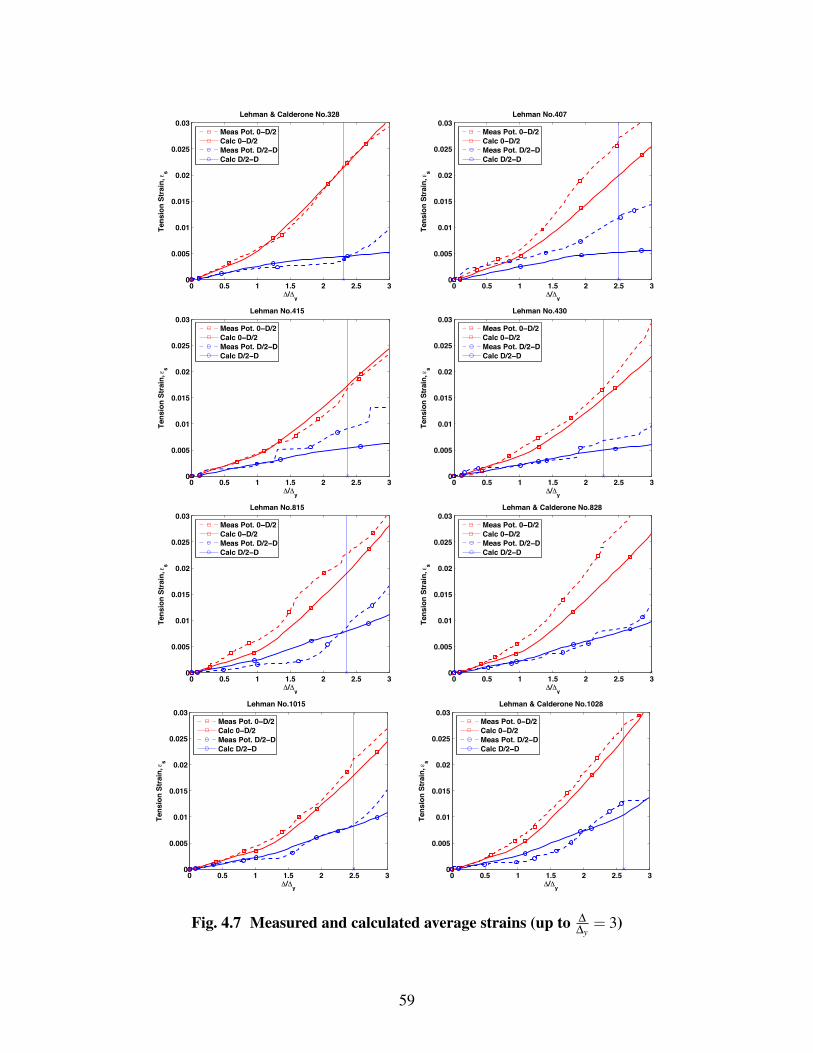
0 0.5 1 1.5 2 2.5 30
0.005
0.01
0.015
0.02
0.025
0.03Lehman & Calderone No.328
∆/∆y
Ten
sio
n S
trai
n, ε
s
Meas Pot. 0−D/2Calc 0−D/2Meas Pot. D/2−DCalc D/2−D
0 0.5 1 1.5 2 2.5 30
0.005
0.01
0.015
0.02
0.025
0.03Lehman No.407
∆/∆y
Ten
sio
n S
trai
n, ε
s
Meas Pot. 0−D/2Calc 0−D/2Meas Pot. D/2−DCalc D/2−D
0 0.5 1 1.5 2 2.5 30
0.005
0.01
0.015
0.02
0.025
0.03Lehman No.415
∆/∆y
Ten
sio
n S
trai
n, ε
s
Meas Pot. 0−D/2Calc 0−D/2Meas Pot. D/2−DCalc D/2−D
0 0.5 1 1.5 2 2.5 30
0.005
0.01
0.015
0.02
0.025
0.03Lehman No.430
∆/∆y
Ten
sio
n S
trai
n, ε
s
Meas Pot. 0−D/2Calc 0−D/2Meas Pot. D/2−DCalc D/2−D
0 0.5 1 1.5 2 2.5 30
0.005
0.01
0.015
0.02
0.025
0.03Lehman No.815
∆/∆y
Ten
sio
n S
trai
n, ε
s
Meas Pot. 0−D/2Calc 0−D/2Meas Pot. D/2−DCalc D/2−D
0 0.5 1 1.5 2 2.5 30
0.005
0.01
0.015
0.02
0.025
0.03Lehman & Calderone No.828
∆/∆y
Ten
sio
n S
trai
n, ε
s
Meas Pot. 0−D/2Calc 0−D/2Meas Pot. D/2−DCalc D/2−D
0 0.5 1 1.5 2 2.5 30
0.005
0.01
0.015
0.02
0.025
0.03Lehman No.1015
∆/∆y
Ten
sio
n S
trai
n, ε
s
Meas Pot. 0−D/2Calc 0−D/2Meas Pot. D/2−DCalc D/2−D
0 0.5 1 1.5 2 2.5 30
0.005
0.01
0.015
0.02
0.025
0.03Lehman & Calderone No.1028
∆/∆y
Ten
sio
n S
trai
n, ε
s
Meas Pot. 0−D/2Calc 0−D/2Meas Pot. D/2−DCalc D/2−D
Fig. 4.7 Measured and calculated average strains (up to ""y
= 3)
59

4.7 SENSITIVITY ANALYSES
A parametric study was performed to verify the results of the optimization analysis and to demon-
strate the effect of the key modeling parameters on model accuracy. In this study, the measures
of accuracy were plotted versus the five modeling parameters to demonstrate the effect of each
parameter (figures 4.8 through 4.12). The optimal solution (b = 0.01, Np = 5, dcomp = c, # = 1.0,
and $ = 0.4) was used as a basis, and each parameter was varied individually.
In Figure 4.8 the effect of the strain hardening ratio is studied by plotting the maximum,
minimum, and mean values of Etotal , S.R., M.R., and D.R. versus the strain-hardening ratio (b).
As seen in the figure, a b value near 1% minimizes the mean Etotal . This result is consistent with
the results of the previous section. As expected, increasing b does not affect the stiffness ratio, but
decreases the M.R. and increases the D.R.
Similarly, the effect of the number of integration points is shown in Figure 4.9. As seen here,
slightly better values of Etotal , M.R., and D.R can be obtained by using 6 or 7 integration points,
but the increase in accuracy does not outweigh the loss of efficiency. As expected, the stiffness
ratio is not affected by Np.
The effect of the bond-strength ratio (#) on pushover accuracy is shown in Figure 4.10. As
expected, as # increases, the stiffness ratios and moment ratios decrease and the degradation error
ratios increase. A negligibly better value of Etotal can be obtained by using # = 0.5 than # = 1.0;
however, the stiffness ratio and moment ratio are better using # = 1.0. The best moment ratio is
obtained by using # = ., which represents no bar slip.
The effect of the bond compression depth (dcomp) on pushover accuracy is shown in Figure
4.11. The stiffness ratios, moment ratios, and degradation error ratios increase as dcomp increases.
The best Etotal value was obtained for dcomp = c, but similar values were obtained for dcomp = 0.1
and 0.2.
Finally, the effect of the shear-deformation ratio ($) is shown in Figure 4.12. As discussed
earlier, the shear ratio influences the accuracy little.
60
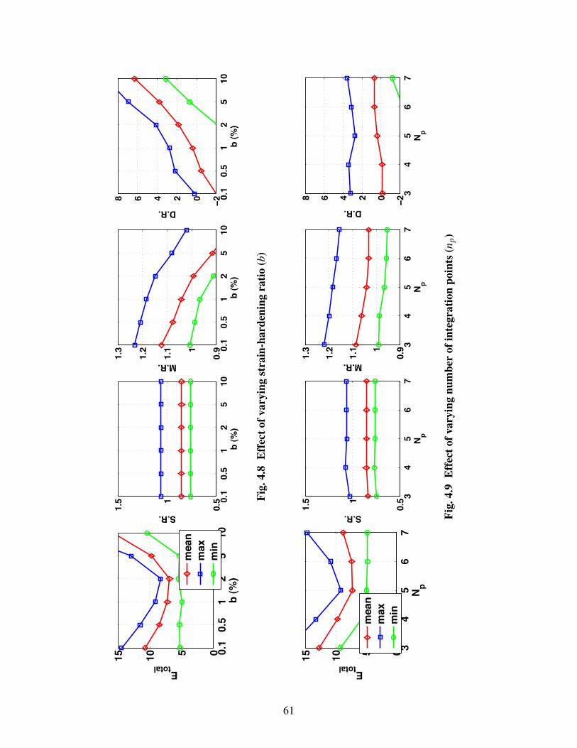
0.1
0.5
12
510
0.51
1.5
b (
%)
S.R.0.
10.
51
25
100.
91
1.1
1.2
1.3
b (
%)
M.R.
0.1
0.5
12
510
−202468
b (
%)
D.R.
0.1
0.5
12
510
051015
b (
%)
Etotal
mea
nm
axm
in
Fig.
4.8
Effe
ctof
vary
ing
stra
in-h
arde
ning
ratio
(b)
34
56
70.51
1.5
Np
S.R.
34
56
70.91
1.1
1.2
1.3
Np
M.R.
34
56
7−202468
Np
D.R.
34
56
7051015
Np
Etotal
mean
max
min
Fig.
4.9
Effe
ctof
vary
ing
num
ber
ofin
tegr
atio
npo
ints
(np)
61

.25
.50.
91
2In
fty
0.51
1.5
Bo
nd−S
tren
gth
Rat
io (λ)
S.R..2
5.5
0.9
12
Inft
y0.
91
1.1
1.2
1.3
Bo
nd−S
tren
gth
Rat
io (λ)
M.R.
.25
.50.
91
2In
fty
−202468
Bo
nd−S
tren
gth
Rat
io (λ)
D.R.
.25
.50.
91
2In
fty
051015
Bo
nd−S
tren
gth
Rat
io (λ)
Etotal
m
ean
max
min
Fig.
4.10
Effe
ctof
vary
ing
bond
-str
engt
hra
tio(#
)
0.1
0.2
0.5
1.0
1.5
0.51
1.5
d comp
S.R.
0.1
0.2
0.5
1.0
1.5
0.91
1.1
1.2
1.3
d comp
M.R.
0.1
0.2
0.5
1.0
1.5
−202468
d comp
D.R.
0.1
0.2
0.5
1.0
1.5
051015
d comp
Etotal
mean
max
min
Fig.
4.11
Effe
ctof
vary
ing
bond
com
pres
sion
dept
h(d
com
p)
62

0.1
0.2
0.4
0.8
1.0
Inft
y0.
51
1.5
Sh
ear−
Sti
ffn
ess
Rat
io (γ
)
S.R.
0.1
0.2
0.4
0.8
1.0
Inft
y0.
91
1.1
1.2
1.3
Sh
ear−
Sti
ffn
ess
Rat
io (γ
)
M.R.
0.1
0.2
0.4
0.8
1.0
Inft
y−20 2 4 6 8
Sh
ear−
Sti
ffn
ess
Rat
io (γ
)
D.R.
0.1
0.2
0.4
0.8
1.0
Inft
y0 5 1015
Sh
ear−
Sti
ffn
ess
Rat
io (γ
)
Etotal
m
ean
max
min
Fig.
4.12
Effe
ctof
vary
ing
shea
r-st
iffne
ssra
tio($
)
63

4.8 EVALUATION WITH DATABASE OF BRIDGE COLUMNS
The proposed modeling strategy was used to model the 37 bridge columns identified in Section
1.3. Key accuracy statistics of this evaluation are provided in Table 4.4. The mean value of the
pushover error Epush was 7.4%. The mean values of the stiffness ratios (S.R.) and moment ratios
(M.R.) were 0.85 and 1.03, with corresponding c.o.v.’s of 15.6% and 7.9%. The mean value of the
degradation ratios (D.R. ) was -0.51.
Table 4.4 Accuracy statistics for envelope response of distributed-plasticity model
Statistic Epush(%) S.R. M.R. D.R.
Mean 7.4 0.84 1.03 -0.51c.o.v. (%) - 15.6 7.9 -
The measures of modeling accuracy are plotted versus key column properties to determine
if the accuracy of the model is sensitive to these properties. In Figure 4.13, Epush is plotted versus,
aspect ratio (L/D), longitudinal-reinforcement ratio ((l), axial-load ratio (P/ f ′cAg), effective con-
finement ratio, concrete compressive strength, and the ratio of spiral spacing to longitudinal bar
diameter (s/db). Included in the figure are the R2 values, which indicate the magnitude of corre-
lation between Epush and the property. As seen in the figure, there are no significant trends in the
data.
Similarly, the stiffness ratio is plotted versus the key column properties in Figure 4.14. Slight
trends can be observed in S.R. versus L/D and f ′c, with R2 values of 0.11 and 0.12.
The maximum moment ratio (M.R.) is plotted versus the key properties in Figure 4.15. As
seen in the figure, only one trend can be observed. The moment ratio decreases with ab increase in
effective confinement ratio.
The degradation ratio (D.R.) is plotted versus the key properties in Figure 4.16. There are no
significant trends in the data.
64

0 2 4 6 8 100
5
10
15
20
L/D
Epush
R2 = 0.014
0 0.01 0.02 0.03 0.040
5
10
15
20
ρl
Epush
R2 = 0.0094
0 0.1 0.2 0.3 0.40
5
10
15
20
P/fcAg
Epush
R2 = 0.0064
0 0.1 0.2 0.30
5
10
15
20
ρeff
Epush
R2 = 0.00028
0 10 20 30 400
5
10
15
20
fc
Epush
R2 = 0.00058
0 1 2 3 4 50
5
10
15
20
S/db
Epush
R2 = 0.018
Fig. 4.13 Effect of key properties on pushover error
65

0 2 4 6 8 100
0.5
1
1.5
L/D
S.R.
R2 = 0.11
0 0.01 0.02 0.03 0.040
0.5
1
1.5
ρl
S.R.
R2 = 0.00022
0 0.1 0.2 0.3 0.40
0.5
1
1.5
P/fcAg
S.R.
R2 = 0.0012
0 0.1 0.2 0.3 0.40
0.5
1
1.5
ρeff
S.R.
R2 = 0.011
0 10 20 30 40 500
0.5
1
1.5
fc
S.R.
R2 = 0.12
0 1 2 3 4 50
0.5
1
1.5
S/db
S.R.
R2 = 0.029
Fig. 4.14 Effect of key properties on stiffness ratio
66

0 2 4 6 8 100
0.5
1
1.5
2
L/D
M.R. R2 = 0.0079
0 0.01 0.02 0.03 0.040
0.5
1
1.5
2
ρl
M.R. R2 = 0.0013
0 0.1 0.2 0.3 0.40
0.5
1
1.5
2
P/fcAg
M.R. R2 = 5.6e−005
0 0.1 0.2 0.30
0.5
1
1.5
2
ρeff
M.R. R2 = 0.2
0 10 20 30 400
0.5
1
1.5
2
fc
M.R. R2 = 0.033
0 1 2 3 4 50
0.5
1
1.5
2
S/db
M.R. R2 = 0.05
Fig. 4.15 Effect of key properties on moment ratio
67

0 2 4 6 8 10−10
−5
0
5
10
L/D
D.R
R2 = 0.072
0 0.01 0.02 0.03 0.04−10
−5
0
5
10
ρl
D.R
R2 = 0.036
0 0.1 0.2 0.3 0.4−10
−5
0
5
10
P/fcAg
D.R
R2 = 0.031
0 0.1 0.2 0.3−10
−5
0
5
10
ρeff
D.R
R2 = 0.015
0 10 20 30 40−10
−5
0
5
10
fc
D.R
R2 = 0.0021
0 1 2 3 4 5−10
−5
0
5
10
S/db
D.R
R2 = 0.032
Fig. 4.16 Effect of key properties on degradation error ratio
68

4.9 SUMMARY
The measures of accuracy and optimization scheme utilized to calibrate the distributed-plasticity
column model were presented in this chapter. The results of the optimization study were then
presented and an optimal solution was selected. The optimal model parameters were as follows.
· Strain-Hardening Ratio, b = 0.01.· Bond-Strength Ratios, #e = 0.9 and #i = 0.45.· Development Bar Stress, )d = 0.25)y.· Number of Integration Points, Np = 5.· Bond-Model Compression Depth, dcomp =1/2 neutral axis depth at 'c = 0.002.· Shear-Stiffness Ratio, $ = 0.4.
This combination of parameters resulted in the following mean measures of accuracy when
applied to the dataset of 8 column tests by Lehman and Moehle (2000): Etotal = 7.22, Epush = 7.02,
E(0−D/4)strain = 6.51, E(D/4−D/2)
strain = 17.73, stiffness ratio = 0.85, moment ratio = 1.04 and degradation
error ratio = 0.38. The corresponding coefficients of variation for the stiffness ratio and moment
ratio were 11% and 8%. When applied to the bridge dataset, the mean value of Epush was 7.4%.
The mean values of the stiffness ratios and moment ratios were 0.85 and 1.03 with corresponding
c.o.v.’s of 15.6% and 7.9%. The mean value of the degradation ratios (D.R. ) was -0.51.
69

5 Development of Lumped-PlasticityColumn Model
The spread-plasticity, force-based fiber beam-column element is susceptible to strain localiza-
tion and loss of objectivity in degrading members (Section 3.1.1). A lumped-plasticity column-
modeling strategy is developed to overcome this limitation, and to provide a less complex model-
ing strategy. In this chapter, a lumped-plasticity model formulation is presented, and key modeling
parameters are identified for calibration.
5.1 MODEL FORMULATIONS
The widespread implementation of nonlinear analysis methods in software to support analysis
and design has led to the development of a variety of plastic-hinge model formulations. In this
chapter, two model formulations are presented, one that is commonly employed in design, and a
more complicated formulation that can be implemented in a standard displacement-based finite
element framework (e.g., OpenSees). Figure 5.1 shows a typical cantilever column subjected to a
lateral load. The figure also shows the moment and actual curvature distributions, and the idealized
curvature distributions that are the basis for the two lumped-plasticity models presented in this
chapter.
The formulation of the plastic-hinge model employed in design uses the idealized distribution
shown in Figure 5.1(d) to develop an expression for the post-yield displacement at the top of
the column, ". The curvature is assumed to be linear above the plastic hinge, and the plastic
curvature is assumed to be constant over the height of the plastic hinge. The resulting post-yield
71

(a) IdealizedColumn
(b) MomentDistribution
(c) ActualCurvature
Distribution
(d) IdealizedCurvature
Distribution forFormulation 1
(e) IdealizedCurvature
Distribution forFormulation 2
Fig. 5.1 Moment and curvature distributions
total displacement can be expressed as follows.
" = "y +(!base−!y)Lp
(L−
Lp
2
)(5.1)
where: !y is the column curvature at first yield, !base is the curvature associated with the moment at
the base of the column, L is the distance from the base of the column to the point of contraflexure,
Lp is the plastic-hinge length, and "y is the yield displacement of the column.
Scott and Fenves (2006) developed a lumped-plasticity formulation suitable for implemen-
tation in a standard displacement-based finite-element environment. The formulation utilizes the
force-based fiber beam-column element formulation, and introduces a modified integration scheme
in which inelastic deformations are confined to an assigned plastic-hinge length. This formulation,
which is available in OpenSees, results in the curvature distribution shown in Figure 5.1(e). The
curvature distribution is linear above the plastic hinge, and within the plastic hinge the curvature is
calculated with moment-curvature analysis. Implementation of this method for a cantilever column
results in the following expression for the post-yield tip displacement.
" =Mbase
(EI)e f f
(L2
3−LLp
)+!baseLLp (5.2)
where: Mbase and !base are the moment and associated curvature at the base of the column, and
72
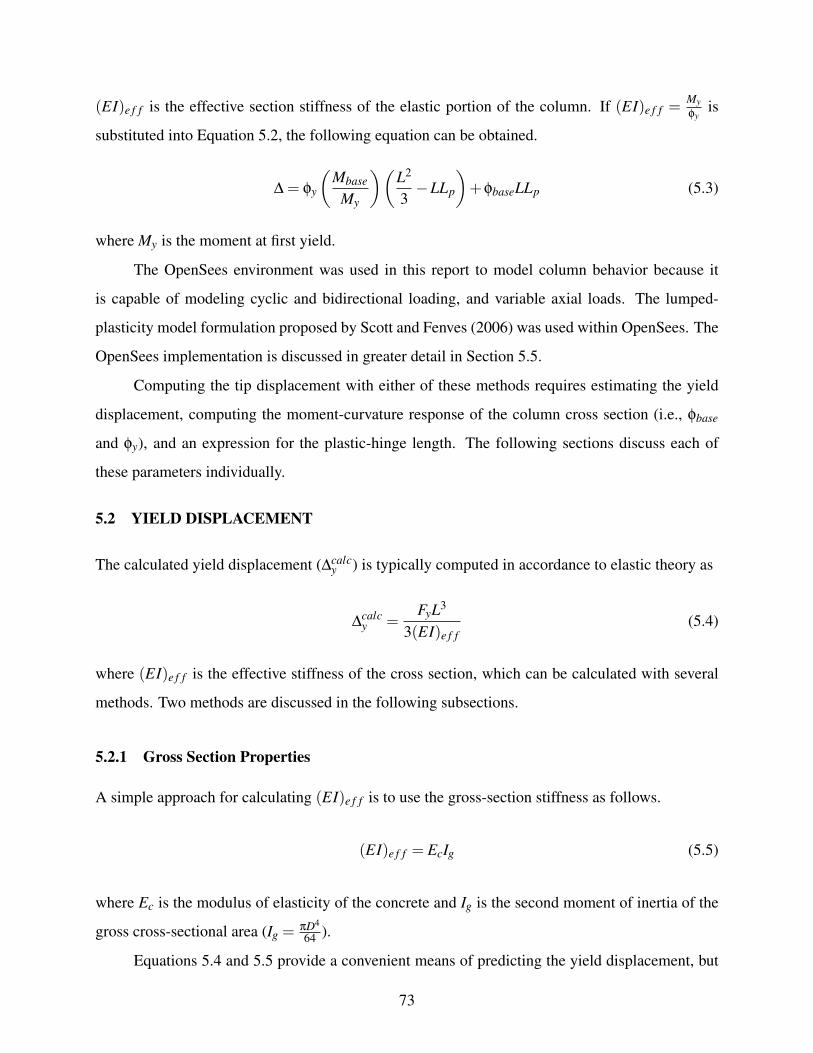
(EI)e f f is the effective section stiffness of the elastic portion of the column. If (EI)e f f = My!y
is
substituted into Equation 5.2, the following equation can be obtained.
" = !y
(Mbase
My
)(L2
3−LLp
)+!baseLLp (5.3)
where My is the moment at first yield.
The OpenSees environment was used in this report to model column behavior because it
is capable of modeling cyclic and bidirectional loading, and variable axial loads. The lumped-
plasticity model formulation proposed by Scott and Fenves (2006) was used within OpenSees. The
OpenSees implementation is discussed in greater detail in Section 5.5.
Computing the tip displacement with either of these methods requires estimating the yield
displacement, computing the moment-curvature response of the column cross section (i.e., !base
and !y), and an expression for the plastic-hinge length. The following sections discuss each of
these parameters individually.
5.2 YIELD DISPLACEMENT
The calculated yield displacement ("calcy ) is typically computed in accordance to elastic theory as
"calcy =
FyL3
3(EI)e f f(5.4)
where (EI)e f f is the effective stiffness of the cross section, which can be calculated with several
methods. Two methods are discussed in the following subsections.
5.2.1 Gross Section Properties
A simple approach for calculating (EI)e f f is to use the gross-section stiffness as follows.
(EI)e f f = EcIg (5.5)
where Ec is the modulus of elasticity of the concrete and Ig is the second moment of inertia of the
gross cross-sectional area (Ig = ,D4
64 ).
Equations 5.4 and 5.5 provide a convenient means of predicting the yield displacement, but
73

they neglect the effects of shear deformation, anchorage slip, and axial load (cracking). A factor
can be introduced to account for these shortcomings of this methodology.
"calcy =
1%g
FyL3
3EIg(5.6)
where %g is the stiffness modification ratio that is to be calibrated with experimental results. This
parameter is studied and calibrated in Section 6.2.
5.2.2 Section Secant Stiffness
Alternatively, (EI)e f f can also be taken as the secant stiffness ((EI)sec) of the column cross section.
The secant stiffness is the slope of the moment-curvature plot up to the yield moment, My.
(EI)e f f = (EI)sec =My
!y(5.7)
This method accounts for the cracking of the column cross section, but assumes that the column is
cracked over the entire height of the column.
Equations 5.4 and 5.7 provide a convenient means of predicting the yield displacement, but
they neglect the effects of shear deformation and anchorage slip. A factor is introduced to account
for these shortcomings of this methodology.
"calcy =
1%sec
FyL3
3(EI)sec(5.8)
where %sec is a stiffness modification ratio that is calibrated with the experimental data described
in Section 6.2.
5.2.3 Expected Trends in %g and %sec
The component of total deformation due to shear is dependent on the aspect ratio of the column,LD . Therefore, %g and %sec are expected to depend on the aspect ratio. The following calculations
are carried out to demonstrate how shear deformation varies with aspect ratio.
74

The flexural component of the yield displacement (" fy ) for a circular cantilever column (Ig =
,D4
64 ) can be calculated as
" fy =
!yL2
3=
MyL2
EcIg=
MyL2
Ec,D4
64
=64L2My
3D4Ec,(5.9)
where L is the length of the column and !y is the yield curvature of the section. The component of
the yield displacement due to shear ("vy) can be calculated as
"vy =
4FyL3GAG
=4My
3GAG=
4My
3G,D2
4
(5.10)
where G is the modulus of rigidity of the concrete, Fy is the lateral shear force, and AG is the gross
area of the section. The ratio of "vy to " f
y can be simplified to the following expression.
"vy
" fy
=Ec
4G( L
D)2 (5.11)
The ratio decreases with increasing aspect ratio, indicating that the fraction of deformation due to
shear decreases with increasing aspect ratio. Therefore, the stiffness modification ratios (%g and
%sec) are expected to increase with increasing aspect ratio.
The following calculations are carried out to study the component of total deformation due
to bond slip. The component of deflection due to bond slip can be approximated as follows.
"by = 0bL (5.12)
where: 0b is base rotation of the column due to bond slip, which can be calculated as
0by =
(ue +u′e)$D
(5.13)
where $ is the ratio of the core diameter (D′) to total column diameter (D), $ = D′
D . ue and u′e are
the vertical displacements of the tensile steel and compressive steel, which can be calculated as
follows (Section 3.2.1).
ue =Ld'y
2(5.14)
75

u′e =L′d'′y
2(5.15)
where: Lp and L′p are the development lengths for the compressive and tensile steel, respectively.
'y is the tensile strain of the reinforcement, and '′y is the strain in the compression reinforcement
when the tensile reinforcement yields, that is
'′y = !y$D− 'y (5.16)
The development lengths (Ld and L′d) of equations 5.14 and 5.15 can be calculated as follows.
Ld =db fy
4&(5.17)
L′d =db f ′y4&
(5.18)
where: & is the bond stress (&≈ 1.0√
f ′c , f ′c in MPa), and db and fy are the diameter and yield stress
of the longitudinal reinforcement, respectively. The yield strain 'y in a column can be approximated
as a function of yield curvature and column depth as follows (Priestley et al. 1996).
'y =D!y
#(5.19)
where: # = 2.45 for spiral-reinforced columns and 2.14 for rectangular-reinforced columns. If
equations 5.13-5.19 are substituted into Equation 5.12 with the identities fy = Es'y and f ′y = Es'′y,
the following expression is obtained for displacement due to bond slip.
"by =
($#($#−2)+2)DEsLdb!2y
8$#2&(5.20)
The ratio of the component of yield displacement due to bond slip to that from flexural deformation
(Equation 5.9) can be calculated as follows.
"by
" fy
=3($#($#−2)+2)
8$#db fy
& L(5.21a)
=3($#($#−2)+2)
2$#Ld
L(5.21b)
76

This ratio increases with an increase in fydb&L ; therefore the fraction of total deformation due to
anchorage slip should increase with this parameter. %g and %sec are therefore expected to decrease
with increasing fydb&L .
In addition to the expected trends discussed above, %g is expected to vary with varying axial-
load ratio ( PAg f ′c
) and longitudinal-reinforcement ratio ((l). EcIg assumes that there is no cracking
in the section, and overestimates the section stiffness. Therefore, %g will be less than 1.0 to reduce
this stiffness. At higher axial loads, %g would not need to reduce EcIg as much because at high
axial loads, the neutral axis depth will be large, and there will be less cracking. Therefore %g is
expected to increase with an increase in axial load. Similarly, there will be less cracking with
higher longitudinal-reinforcement ratios, therefore al phag is expected to increase with increase in
(l .
Table 5.1 summarizes the expected trends in the stiffness modification ratios.
Table 5.1 Expected trends in %
LD
PAg f ′c
fydbL& (l
%g ↑ ↑ ↓ ↑%sec ↑ - ↓ -
5.3 MOMENT-CURVATURE RESPONSE
For this study, the cross sections of the columns were modeled with fiber sections (Section 2.1).
With a fiber section, the column cross section is divided into small fibers in which each fiber is
assigned a particular stress-strain response depending on the material the fiber represents. The
fiber-section discretization strategies developed in Section 2.3 and the material models described
in Section 2.2 were used to model the moment-curvature response of the lumped-plasticity models.
5.4 PLASTIC-HINGE LENGTHS
Many models have been proposed to estimate the plastic-hinge length based on the column prop-
erties. Previous researchers (e.g., Priestley et al. (1996); Mattock (1967)) have proposed that the
plastic-hinge length is proportional to the column length, L, column depth, D, and the longitudinal
77

reinforcement properties, as in the following equation:
Lp = 11L+12D+13 fydb (5.22)
where fy and db are the yield stress and bar diameter of the tension reinforcement, respectively. The
column length is included in Equation 5.22 to account for the moment gradient along the length of
the cantilever, and the column depth is included to account for the influence of shear on the size
of the plastic region. The properties of the longitudinal bars are included to account for additional
rotation at the plastic hinge resulting from anchorage bond slip.
Priestley et al. (1996) proposed an equation to calculate the plastic-hinge length in columns,
in which 11 = 0.08, 12 = 0, and 13 = 0.022 (fy in MPa) with an upper limit on Lp of 0.044 fydb.
Mattock (1967) proposed an equation to calculate the plastic-hinge length in beams, in which
11 = 120 , 12 = 1
2 , and 13 = 0.0.
Equation 5.23 provides a reasonable estimate of column plastic-hinge length; however it can
be shown that the amount of deformation due to bond slip is expected to vary with fydb√f ′c
and not
just fydb. Therefore, the following modification to Equation 5.22 is proposed.
Lp = 11L+12D+13fydb√
f ′c(5.23)
Equation 5.23 is used in this research to represent the length of plastic hinges. The unknown
parameters (11, 12, and 13) are calibrated with experimental results in Chapter 6. Upon completion
of the calibration, the effect of using the general form of plastic-hinge length proposed by Equation
5.22 will be evaluated.
5.5 OPENSEES IMPLEMENTATION
The OpenSees implementation of the lumped-plasticity model was used in this report because
OpenSees is capable of modeling cyclic and bidirectional loading, and variable axial loads. For
this research, the lumped-plasticity integration scheme proposed by Scott and Fenves (2006) is
used within OpenSees. The current version of OpenSees (version 1.6.2.f) has three formulations
of lumped-plasticity models. The formulation discussed in Section 5.1 (Scott and Fenves 2006)
is used with the beamWithHinges3 command in OpenSees. This command takes as input the
78
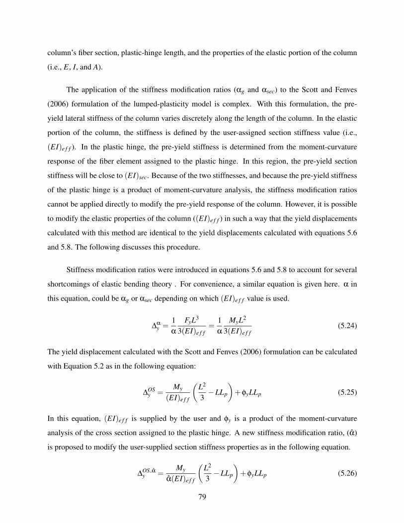
column’s fiber section, plastic-hinge length, and the properties of the elastic portion of the column
(i.e., E, I, and A).
The application of the stiffness modification ratios (%g and %sec) to the Scott and Fenves
(2006) formulation of the lumped-plasticity model is complex. With this formulation, the pre-
yield lateral stiffness of the column varies discretely along the length of the column. In the elastic
portion of the column, the stiffness is defined by the user-assigned section stiffness value (i.e.,
(EI)e f f ). In the plastic hinge, the pre-yield stiffness is determined from the moment-curvature
response of the fiber element assigned to the plastic hinge. In this region, the pre-yield section
stiffness will be close to (EI)sec. Because of the two stiffnesses, and because the pre-yield stiffness
of the plastic hinge is a product of moment-curvature analysis, the stiffness modification ratios
cannot be applied directly to modify the pre-yield response of the column. However, it is possible
to modify the elastic properties of the column ((EI)e f f ) in such a way that the yield displacements
calculated with this method are identical to the yield displacements calculated with equations 5.6
and 5.8. The following discusses this procedure.
Stiffness modification ratios were introduced in equations 5.6 and 5.8 to account for several
shortcomings of elastic bending theory . For convenience, a similar equation is given here. % in
this equation, could be %g or %sec depending on which (EI)e f f value is used.
"%y =
1%
FyL3
3(EI)e f f=
1%
MyL2
3(EI)e f f(5.24)
The yield displacement calculated with the Scott and Fenves (2006) formulation can be calculated
with Equation 5.2 as in the following equation:
"OSy =
My
(EI)e f f
(L2
3−LLp
)+!yLLp (5.25)
In this equation, (EI)e f f is supplied by the user and !y is a product of the moment-curvature
analysis of the cross section assigned to the plastic hinge. A new stiffness modification ratio, (%̂)
is proposed to modify the user-supplied section stiffness properties as in the following equation.
"OS %̂y =
My
%̂(EI)e f f
(L2
3−LLp
)+!yLLp (5.26)
79

An expression for %̂ can be obtained by setting equations 5.24 and 5.26 equal to each other and
simplifying. The resulting equation is as follows.
%̂ =%(L−3Lp)My
LMy−3%(EI)e f f Lp!y(5.27)
This expression can be used for % = %g and (EI)e f f = EcIg, as well as for % = %sec and (EI)e f f =
(EI)sec. The expression for %̂sec can be simplified further by substituting the identities !y = My(EI)sec
(see Equation 5.7) and (EI)e f f = (EI)sec into Equation 5.27.
%̂sec =%(L−3Lp)L−3%Lp
(5.28)
5.6 SUMMARY
In this chapter, two formulations of the lumped-plasticity column-modeling strategy were pre-
sented, and key modeling parameters were identified for calibration with experimental results. The
following parameters were identified for calibration and are calibrated in Chapter 6.
Stiffness Modification Ratios, %g, %sec. The parameters that account for several shortcomings of
elastic theory at predicting yield displacement, "calcy = "elastic
y%g/sec
(Section 5.2).
Plastic-Hinge-Length Parameters, 11, 12, and 13. The parameters used in the plastic-hinge-length
equation; Lp = 11L+12D+13fydb√
f ′c(Section 5.4).
80

6 Calibration of Lumped-PlasticityColumn Model
To accurately model the force-deformation response of reinforced concrete columns with the lumped-
plasticity modeling strategy, the modeling parameters identified in Chapter 5 were calibrated with
experimental results. The modeling parameters identified for calibration were:
Stiffness Modification Ratios, %g, %sec. The parameters that account for several shortcomings of
elastic theory at predicting yield displacement, "calcy = "elastic
y%g/sec
(Section 5.2).
Plastic-Hinge-Length Parameters, 11, 12, and 13. The parameters used in the plastic-hinge-length
equation: Lp = 11L+12D+13fydb√
f ′c(Section 5.4).
This chapter discusses the calibration of the stiffness modification ratios and presents the
results of this study. The optimization strategy used to calibrate the plastic-hinge-length equation
is then presented, and the results of the calibration are summarized. The results of a sensitivity
analysis are then presented to identify the effects of varying key parameters.
6.1 MEASURES OF ACCURACY
The parameters used in this chapter to measure the accuracy of the lumped-plasticity modeling
strategy are identical to the measures used for the distributed-plasticity model, with the exception
that the distributed-plasticity model accounted for the strain error Estrain. The measures are as
follows:
81
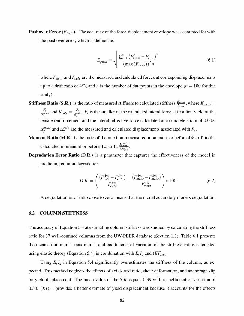
Pushover Error (Epush). The accuracy of the force-displacement envelope was accounted for with
the pushover error, which is defined as
Epush =
√√√√-ni=1
(Fi
meas−Ficalc
)2
(max(Fmeas))2 n(6.1)
where Fmeas and Fcalc are the measured and calculated forces at corresponding displacements
up to a drift ratio of 4%, and n is the number of datapoints in the envelope (n = 100 for this
study).
Stiffness Ratio (S.R.) is the ratio of measured stiffness to calculated stiffness KmeasKcalc
, where Kmeas =Fy
"measy
and Kcalc = Fy"calc
y. Fy is the smaller of the calculated lateral force at first first yield of the
tensile reinforcement and the lateral, effective force calculated at a concrete strain of 0.002.
"measy and "calc
y are the measured and calculated displacements associated with Fy.
Moment Ratio (M.R) is the ratio of the maximum measured moment at or before 4% drift to the
calculated moment at or before 4% drift, Mmeasmax
Mcalcmax
.
Degradation Error Ratio (D.R.) is a parameter that captures the effectiveness of the model in
predicting column degradation.
D.R. =
((F4%
calc−F3%calc
)
F3%calc
−(F4%
meas−F3%meas
)
F3%meas
)∗100 (6.2)
A degradation error ratio close to zero means that the model accurately models degradation.
6.2 COLUMN STIFFNESS
The accuracy of Equation 5.4 at estimating column stiffness was studied by calculating the stiffness
ratio for 37 well-confined columns from the UW-PEER database (Section 1.3). Table 6.1 presents
the means, minimums, maximums, and coefficients of variation of the stiffness ratios calculated
using elastic theory (Equation 5.4) in combination with EcIg and (EI)sec.
Using EcIg in Equation 5.4 significantly overestimates the stiffness of the column, as ex-
pected. This method neglects the effects of axial-load ratio, shear deformation, and anchorage slip
on yield displacement. The mean value of the S.R. equals 0.39 with a coefficient of variation of
0.30. (EI)sec provides a better estimate of yield displacement because it accounts for the effects
82
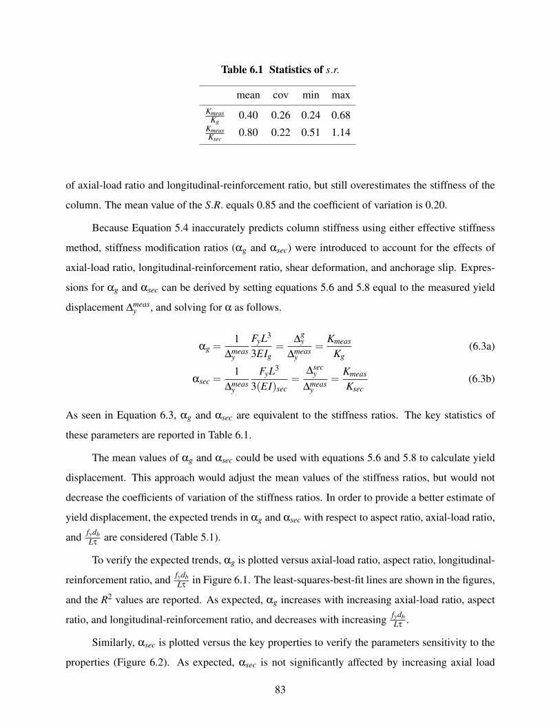
Table 6.1 Statistics of s.r.
mean cov min maxKmeas
Kg0.40 0.26 0.24 0.68
KmeasKsec
0.80 0.22 0.51 1.14
of axial-load ratio and longitudinal-reinforcement ratio, but still overestimates the stiffness of the
column. The mean value of the S.R. equals 0.85 and the coefficient of variation is 0.20.
Because Equation 5.4 inaccurately predicts column stiffness using either effective stiffness
method, stiffness modification ratios (%g and %sec) were introduced to account for the effects of
axial-load ratio, longitudinal-reinforcement ratio, shear deformation, and anchorage slip. Expres-
sions for %g and %sec can be derived by setting equations 5.6 and 5.8 equal to the measured yield
displacement "measy , and solving for % as follows.
%g =1
"measy
FyL3
3EIg=
"gy
"measy
=Kmeas
Kg(6.3a)
%sec =1
"measy
FyL3
3(EI)sec=
"secy
"measy
=Kmeas
Ksec(6.3b)
As seen in Equation 6.3, %g and %sec are equivalent to the stiffness ratios. The key statistics of
these parameters are reported in Table 6.1.
The mean values of %g and %sec could be used with equations 5.6 and 5.8 to calculate yield
displacement. This approach would adjust the mean values of the stiffness ratios, but would not
decrease the coefficients of variation of the stiffness ratios. In order to provide a better estimate of
yield displacement, the expected trends in %g and %sec with respect to aspect ratio, axial-load ratio,
and fydbL& are considered (Table 5.1).
To verify the expected trends, %g is plotted versus axial-load ratio, aspect ratio, longitudinal-
reinforcement ratio, and fydbL& in Figure 6.1. The least-squares-best-fit lines are shown in the figures,
and the R2 values are reported. As expected, %g increases with increasing axial-load ratio, aspect
ratio, and longitudinal-reinforcement ratio, and decreases with increasing fydbL& .
Similarly, %sec is plotted versus the key properties to verify the parameters sensitivity to the
properties (Figure 6.2). As expected, %sec is not significantly affected by increasing axial load
83

0 0.05 0.1 0.15 0.2 0.25 0.3 0.350
0.2
0.4
0.6
0.8
1
R2 = 0.16
P/Agfc
αg
0 2 4 6 8 100
0.2
0.4
0.6
0.8
1
R2 = 0.14
L/D
αg
0 0.2 0.4 0.6 0.8 1 1.2 1.4 1.60
0.2
0.4
0.6
0.8
1
R2 = 0.14
fy d
b/L τ
αg
0 0.005 0.01 0.015 0.02 0.025 0.03 0.035 0.040
0.2
0.4
0.6
0.8
1
R2 = 0.17
ρl
αg
Fig. 6.1 %g versus key column properties
and longitudinal-reinforcement ratio because (EI)sec already accounts for the effects of cracking.
However, as expected, %sec increases with increasing aspect ratio and decreases with increasingfydbL& .
Based on these trends, simple expressions were developed for %g and %sec as functions of
aspect ratio, axial-load ratio, longitudinal-reinforcement ratio, and fydbL& . The general form of the
expressions were as follows:
%calcg/sec = #1 +#2
LD
+#3P
Ag f ′c+#4
fydb
L&+#5(l ≤ 1.0 (6.4)
The parameters #1-#5 were calibrated for both cross-section stiffness methods using the 37
84
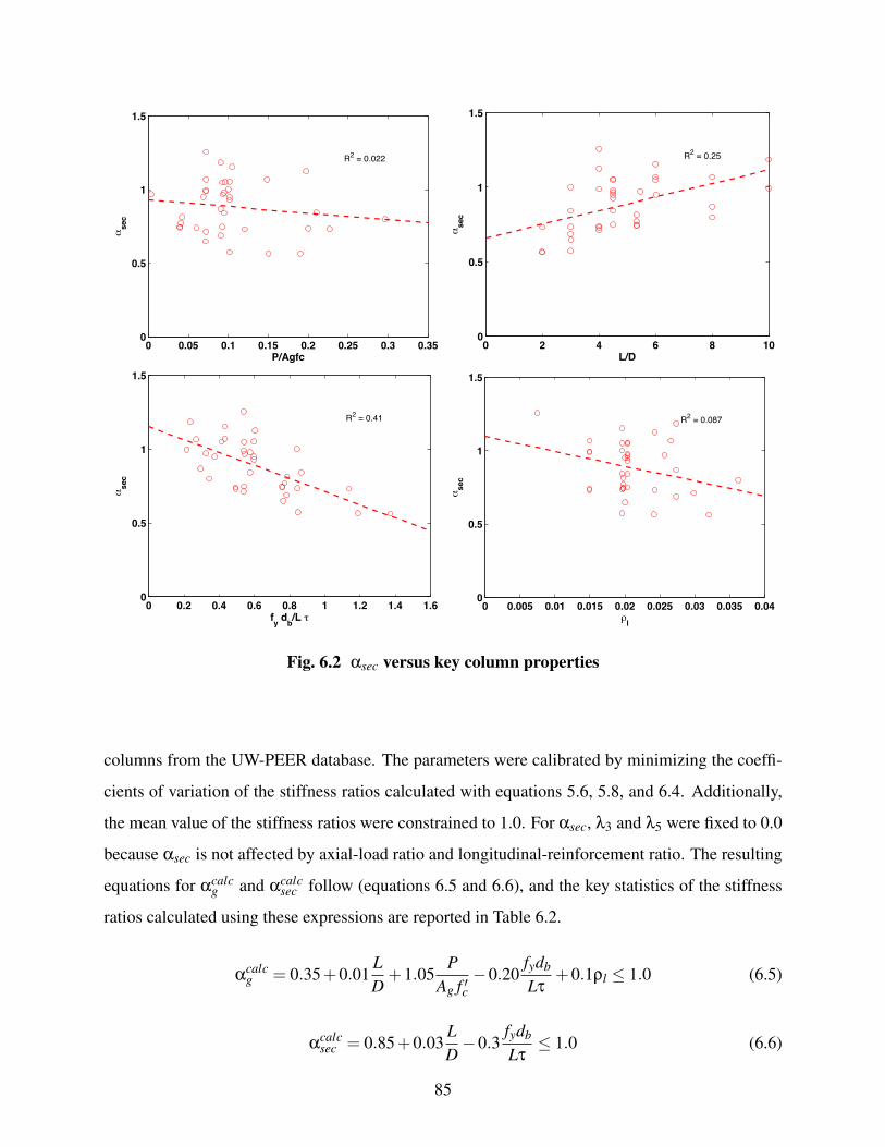
0 0.05 0.1 0.15 0.2 0.25 0.3 0.350
0.5
1
1.5
R2 = 0.022
P/Agfc
αsec
0 2 4 6 8 100
0.5
1
1.5
R2 = 0.25
L/D
αsec
0 0.2 0.4 0.6 0.8 1 1.2 1.4 1.60
0.5
1
1.5
R2 = 0.41
fy d
b/L τ
αse
c
0 0.005 0.01 0.015 0.02 0.025 0.03 0.035 0.040
0.5
1
1.5
R2 = 0.087
ρl
αsec
Fig. 6.2 %sec versus key column properties
columns from the UW-PEER database. The parameters were calibrated by minimizing the coeffi-
cients of variation of the stiffness ratios calculated with equations 5.6, 5.8, and 6.4. Additionally,
the mean value of the stiffness ratios were constrained to 1.0. For %sec, #3 and #5 were fixed to 0.0
because %sec is not affected by axial-load ratio and longitudinal-reinforcement ratio. The resulting
equations for %calcg and %calc
sec follow (equations 6.5 and 6.6), and the key statistics of the stiffness
ratios calculated using these expressions are reported in Table 6.2.
%calcg = 0.35+0.01
LD
+1.05P
Ag f ′c−0.20
fydb
L&+0.1(l ≤ 1.0 (6.5)
%calcsec = 0.85+0.03
LD−0.3
fydb
L&≤ 1.0 (6.6)
85
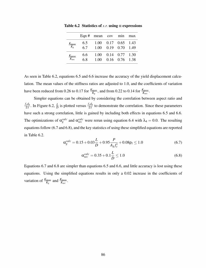
Table 6.2 Statistics of s.r. using % expressions
Eqn # mean cov min max
KmeasKg
6.5 1.00 0.17 0.65 1.436.7 1.00 0.19 0.70 1.49
KmeasKsec
6.6 1.00 0.14 0.77 1.306.8 1.00 0.16 0.76 1.38
As seen in Table 6.2, equations 6.5 and 6.6 increase the accuracy of the yield displacement calcu-
lation. The mean values of the stiffness ratios are adjusted to 1.0, and the coefficients of variation
have been reduced from 0.26 to 0.17 for KmeasKg
, and from 0.22 to 0.14 for KmeasKsec
.
Simpler equations can be obtained by considering the correlation between aspect ratio andfydbL& . In Figure 6.2, L
D is plotted versus fydbL& to demonstrate the correlation. Since these parameters
have such a strong correlation, little is gained by including both effects in equations 6.5 and 6.6.
The optimizations of %calcg and %calc
sec were rerun using equation 6.4 with #4 = 0.0. The resulting
equations follow (6.7 and 6.8), and the key statistics of using these simplified equations are reported
in Table 6.2.
%calcg = 0.15+0.03
LD
+0.95P
Ag f ′c+0.08(l ≤ 1.0 (6.7)
%calcsec = 0.35+0.1
LD≤ 1.0 (6.8)
Equations 6.7 and 6.8 are simpler than equations 6.5 and 6.6, and little accuracy is lost using these
equations. Using the simplified equations results in only a 0.02 increase in the coefficients of
variation of KmeasKg
and KmeasKsec
.
86

0 0.2 0.4 0.6 0.8 1 1.2 1.4 1.60
2
4
6
8
10
R2 = 0.62
fy d
b/L τ
L/D
Fig. 6.3 Correlation between ld and fydb
l&
6.3 CALIBRATION OF PLASTIC-HINGE LENGTH
The general form of an expression to estimate plastic-hinge length was proposed in Section 5.4
(Equation 5.23). The expression is given again here with a limit of L4 . The limit on the plastic-hinge
length is from the lumped-plasticity model formulation proposed by Scott and Fenves (2006).
Lp = 11L+12D+13fydb√
f ′c<=
L4
(6.9)
The parameters 11, 12, and 13 are calibrated with experimental results in this section.
6.3.1 Optimization Scheme
The optimization was performed by running pushover analyses for a broad range of calibration
parameters (11, 12, 13) and then selecting the scheme in which the total error (Etotal , Equation 6.10)
was minimized and the additional modeling accuracy terms (e.g., stiffness ratio) were reasonable.
The range of values used for each calibration parameter are shown in Table 6.3, along with the step
size between consecutive values within the range. The analysis consisted of every combination of
the optimization parameters, which amounted to ∼5,000 combinations.
The optimization scheme used for this modeling strategy couples the accuracy of force-
deformation predictions with the accuracy damage progression predictions. The total error, Etotal ,
87

Table 6.3 Calibration parameter ranges for plastic-hinge length
parameter 11 12 13
min 0 0 0max 0.2 0.8 0.15step size 0.0125 0.0500 0.01
is defined as
Etotal =mean
(Epush
)
2+
/1
4cov
("meas
bb"calc
bb
)+
/2
4cov
("meas
sp
"calcsp
)(6.10)
where: "meassp is the observed displacement at the onset of cover spalling, and "calc
sp is the calculated
displacement associated with the mean value of the maximum compressive strain in the concrete
at cover spalling, 'meansp . "meas
bb is the observed displacement at the onset of bar buckling, and
"calcbb is the calculated displacement associated with the calculated tensile strain in the longitudinal
reinforcement at the onset of bar buckling, 'calcbb . This buckling strain is to be calculated as a
function of the effective confinement ratio ((e f f ) to account for the effect of spiral reinforcement
on bar buckling, as in the following equation (Berry and Eberhard 2005).
'calcbb = 21 +22(e f f ≤ 0.15 (6.11)
where: (e f f = (s fysf ′c
, and 21 and 22 are to be calibrated by minimizing the coefficient of variation
of 'bb'calc
bb. 'bb is the calculated tensile strain at the onset of bar buckling associated with the observed
displacement of bar buckling.
The / terms in Equation 6.10 are included to ensure that the error terms are of similar mag-
nitude.
/1 =min
(mean
(Epush
))
min(
cov(
"measbb
"calcbb
)) (6.12)
/2 =min
(mean
(Epush
))
min(
cov("meas
sp"calc
sp
)) (6.13)
In equations 6.10, 6.12, and 6.13 mean entails the average value for the 37 bridge columns, cov is
the coefficient of variation of for the columns in which the particular damage state is available (i.e.,
33 columns for bar buckling and 31 columns for spalling), and min entails the minimum value out
88

of the total number of combinations.
This optimization scheme did not account for the accuracy of the local deformations in the
same manner as the optimization scheme used for the distributed-plasticity modeling strategy. This
is because the local deformations in the plastic hinge are average values over the height of the
plastic hinge. These average values do not correlate to available measured strain and rotation data.
OpenSees was used to model the the columns using the lumped-plasticity formulation pro-
posed by Scott and Fenves (2006) (Section 5.1). The plastic hinges in this study were assigned
fiber sections with the uniform-radial section discretization scheme described in Section 2.3. The
steel was modeled with the Giufre-Menegotto-Pinto model described in Section 2.2.1. The strain-
hardening ratio, b was set to 0.01. The Popovics curve with model parameters proposed by Mander
et al. (1988) was used to model both the confined and unconfined concrete (Section 2.2.2). Addi-
tionally, the section stiffnesses of the elastic portion of the columns were calculated as the secant
stiffnesses multiplied by the stiffness modification ratios (i.e., (EI)e f f = %̂sec(EI)sec, Section 6.2).
%sec was calculated with Equation 6.8, and %̂sec was then calculated with Equation 5.28.
6.3.2 Optimization Results
The optimization study described in the previous section was performed for 37 columns from
the UW-PEER database (Section 4.1). The top 20 combinations from the optimization study are
reported in Table 6.4. It should be noted that the stiffness ratios for all plastic-hinge lengths were
1.0 because the stiffness modification ratio %̂sec was used in this study to adjust the elastic stiffness
properties of the column ((EI)e f f ).
The combination that minimized Etotal was 11 = 0.0375, 12 = 0, and 13 = 0.12 (Etotal =
8.05). However, for simplicity, the combination in which 11 = 0.05, 12 = 0, and 13 = 0.1 (Etotal =
8.09) was chosen as the optimal solution (combination #13). In Table 6.5, the chosen optimal
solution is compared to the overall optimal solution, and the plastic-hinge models proposed by
Priestley et al. (1996), Mattock (1967), and Corley (1966).
89

Tabl
e6.
4Lu
mpe
d-pl
astic
ityop
timiz
atio
nre
sults
Para
met
erVa
lues
Push
over
Acc
urac
yD
amag
eEs
timat
es
Ran
k1 1
1 21 3
E tot
alE
push
M.R
.D
.R.
' bb
'calc
bb"m
eas
bb "calc
bb' s
p"m
eas
sp "mea
nsp
mea
nm
ean
mea
nm
ean
mea
nco
v2 1
2 2co
vm
ean
cov
cov
10.
040.
000.
108.
533
8.46
11.
058
-0.6
380.
091
0.29
70.
054
0.25
60.
244
0.00
90.
483
0.33
82
0.04
0.00
0.11
8.53
78.
460
1.06
2-0
.563
0.08
60.
296
0.05
20.
236
0.24
50.
009
0.47
60.
338
30.
040.
000.
128.
552
8.47
31.
065
-0.6
010.
082
0.29
60.
050
0.22
00.
246
0.00
80.
470
0.33
84
0.04
0.00
0.09
8.56
08.
500
1.05
3-0
.700
0.09
60.
299
0.05
60.
277
0.24
50.
010
0.49
20.
339
50.
040.
050.
098.
566
8.44
31.
061
-0.5
980.
087
0.29
80.
053
0.23
40.
249
0.00
90.
477
0.33
86
0.04
0.05
0.08
8.57
18.
450
1.05
8-0
.640
0.09
10.
300
0.05
50.
253
0.24
90.
009
0.48
40.
339
70.
050.
000.
098.
572
8.46
01.
062
-0.7
800.
085
0.30
20.
048
0.26
00.
244
0.00
90.
486
0.34
48
0.05
0.00
0.10
8.57
48.
477
1.06
6-0
.704
0.08
10.
300
0.04
60.
241
0.24
40.
008
0.47
90.
344
90.
040.
000.
138.
575
8.49
21.
068
-0.6
950.
078
0.29
60.
049
0.20
50.
247
0.00
80.
463
0.33
810
0.04
0.05
0.10
8.57
98.
465
1.06
5-0
.589
0.08
20.
297
0.05
10.
218
0.24
90.
008
0.47
00.
338
110.
050.
000.
118.
580
8.49
61.
069
-0.7
280.
078
0.29
70.
045
0.22
50.
244
0.00
80.
471
0.34
412
0.05
0.00
0.12
8.58
38.
517
1.07
2-0
.844
0.07
40.
296
0.04
40.
210
0.24
30.
008
0.46
50.
343
130.
030.
000.
128.
595
8.47
51.
057
-0.4
360.
092
0.30
10.
059
0.22
90.
254
0.00
90.
477
0.33
314
0.05
0.00
0.13
8.59
78.
551
1.07
5-0
.978
0.07
10.
295
0.04
30.
197
0.24
30.
007
0.45
90.
342
150.
040.
000.
148.
598
8.51
91.
071
-0.8
490.
075
0.29
60.
047
0.19
20.
249
0.00
80.
458
0.33
816
0.05
0.00
0.08
8.60
08.
473
1.05
9-0
.791
0.09
00.
306
0.04
90.
282
0.24
60.
009
0.49
50.
345
170.
040.
050.
118.
600
8.48
71.
069
-0.7
140.
079
0.29
70.
049
0.20
40.
250
0.00
80.
464
0.33
918
0.03
0.00
0.11
8.60
38.
509
1.05
2-0
.604
0.09
80.
300
0.06
20.
248
0.25
30.
010
0.48
40.
333
190.
040.
000.
088.
605
8.56
61.
048
-0.7
380.
102
0.30
10.
058
0.30
40.
245
0.01
00.
501
0.34
020
0.04
0.05
0.07
8.60
88.
487
1.05
3-0
.613
0.09
60.
302
0.05
70.
274
0.25
00.
010
0.49
20.
340
90

Tabl
e6.
5C
ompa
riso
nof
lum
ped-
plas
ticity
mod
els
Tota
lAcc
urac
yPu
shov
erA
ccur
acy
Bar
Buc
klin
gEs
timat
esSp
allin
gEs
timat
es
Plas
tic-H
inge
Leng
thE t
otal
(%)o
fEto
tal
Epu
shM
.R.
D.R
.' b
b"m
eas
bb "mea
nbb
2 12 2
"mea
sbb "ca
lcbb
' sp
"mea
ssp "m
ean
sp
mea
nE
push
E bb
E sp
mea
nm
ean
mea
nm
ean
cov
cov
cov
mea
nco
vco
v
Ove
rall
Opt
imal
0.03
75L
+0.
11f y
d b√
f′ c≤
L/4
8.05
30.
488
0.24
50.
267
7.85
81.
047
-1.1
500.
083
0.29
40.
277
0.05
00.
224
0.23
90.
008
0.47
10.
344
Sele
cted
Opt
imal
0.05
L+
0.1
f yd b
√f′ c≤
L/4
8.08
90.
486
0.24
30.
272
7.85
61.
048
-1.1
490.
082
0.29
90.
282
0.04
60.
246
0.23
70.
008
0.48
20.
352
Prie
stle
yet
al.(
1996
)0.
08L
+0.
022
f yd b≤
0.04
4f y
d b8.
472
0.46
40.
275
0.26
18.
041
1.05
9-1
.235
0.07
00.
349
0.32
20.
040
0.20
50.
281
0.00
70.
455
0.35
5
Mat
tock
(196
7)0.
05L
+0.
5D8.
900
0.44
10.
318
0.24
18.
047
1.05
1-1
.127
0.08
30.
375
0.34
70.
067
0.11
00.
342
0.00
80.
458
0.34
3
Cor
ley
(196
6)0.
5D8.
545
0.46
00.
282
0.25
88.
153
1.06
9-1
.364
0.05
80.
323
0.30
50.
041
0.11
90.
291
0.00
60.
422
0.35
4
91
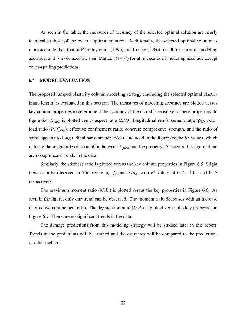
As seen in the table, the measures of accuracy of the selected optimal solution are nearly
identical to those of the overall optimal solution. Additionally, the selected optimal solution is
more accurate than that of Priestley et al. (1996) and Corley (1966) for all measures of modeling
accuracy, and is more accurate than Mattock (1967) for all measures of modeling accuracy except
cover-spalling predictions.
6.4 MODEL EVALUATION
The proposed lumped-plasticity column-modeling strategy (including the selected optimal plastic-
hinge length) is evaluated in this section. The measures of modeling accuracy are plotted versus
key column properties to determine if the accuracy of the model is sensitive to these properties. In
figure 6.4, Epush is plotted versus aspect ratio (L/D), longitudinal-reinforcement ratio ((l), axial-
load ratio (P/ f ′cAg), effective confinement ratio, concrete compressive strength, and the ratio of
spiral spacing to longitudinal bar diameter (s/db). Included in the figure are the R2 values, which
indicate the magnitude of correlation between Epush and the property. As seen in the figure, there
are no significant trends in the data.
Similarly, the stiffness ratio is plotted versus the key column properties in Figure 6.5. Slight
trends can be observed in S.R. versus (l , f ′c, and s/db, with R2 values of 0.12, 0.11, and 0.15
respectively.
The maximum moment ratio (M.R.) is plotted versus the key properties in Figure 6.6. As
seen in the figure, only one trend can be observed. The moment ratio decreases with an increase
in effective-confinement ratio. The degradation ratio (D.R.) is plotted versus the key properties in
Figure 6.7. There are no significant trends in the data.
The damage predictions from this modeling strategy will be studied later in this report.
Trends in the predictions will be studied and the estimates will be compared to the predictions
of other methods.
92

0 5 100
5
10
15
20R2 = 0.0037
L/D
Epush
0 0.01 0.02 0.03 0.040
5
10
15
20R2 = 0.0037
ρl
Epush
0 0.1 0.2 0.3 0.40
5
10
15
20R2 = 0.00026
P/fcAg
Epush
0 0.1 0.20
5
10
15
20R2 = 0.0011
ρeff
Epush
0 20 40 600
5
10
15
20R2 = 0.046
fc
Epush
0 1 2 3 4 50
5
10
15
20R2 = 0.024
S/db
Epush
Fig. 6.4 Effect of key properties on pushover error
93

0 5 100
0.5
1
1.5
2R2 = 0.0036
L/D
S.R.
0 0.01 0.02 0.03 0.040
0.5
1
1.5
2R2 = 0.12
ρl
S.R.
0 0.1 0.2 0.3 0.40
0.5
1
1.5
2R2 = 0.0023
P/fcAg
S.R.
0 0.1 0.2 0.3 0.40
0.5
1
1.5
2R2 = 1.1e−006
ρeff
S.R.
0 20 40 60 800
0.5
1
1.5
2R2 = 0.11
fc
S.R.
0 1 2 3 4 50
0.5
1
1.5
2R2 = 0.15
S/db
S.R.
Fig. 6.5 Effect of key properties on stiffness ratio
94

0 5 100
0.5
1
1.5
2
R2 = 0.0035
L/D
M.R.
0 0.01 0.02 0.03 0.040
0.5
1
1.5
2
R2 = 0.0038
ρl
M.R.
0 0.1 0.2 0.3 0.40
0.5
1
1.5
2
R2 = 0.0047
P/fcAg
M.R.
0 0.1 0.20
0.5
1
1.5
2
R2 = 0.16
ρeff
M.R.
0 20 40 600
0.5
1
1.5
2
R2 = 0.027
fc
M.R.
0 1 2 3 4 50
0.5
1
1.5
2
R2 = 0.042
S/db
M.R.
Fig. 6.6 Effect of key properties on moment ratio
95

0 5 10−10
−5
0
5
10
R2 = 0.011
L/D
D.R
0 0.01 0.02 0.03 0.04−10
−5
0
5
10
R2 = 0.029
ρl
D.R
0 0.1 0.2 0.3 0.4−10
−5
0
5
10
R2 = 0.042
P/fcAg
D.R
0 0.1 0.2−10
−5
0
5
10
R2 = 0.058
ρeff
D.R
0 20 40 60−10
−5
0
5
10
R2 = 0.022
fc
D.R
0 1 2 3 4 5−10
−5
0
5
10
R2 = 0.083
S/db
D.R
Fig. 6.7 Effect of key properties on degradation error ratio
96
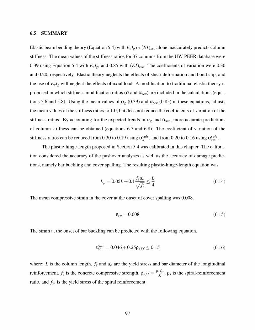
6.5 SUMMARY
Elastic beam bending theory (Equation 5.4) with EcIg or (EI)sec alone inaccurately predicts column
stiffness. The mean values of the stiffness ratios for 37 columns from the UW-PEER database were
0.39 using Equation 5.4 with EcIg, and 0.85 with (EI)sec. The coefficients of variation were 0.30
and 0.20, respectively. Elastic theory neglects the effects of shear deformation and bond slip, and
the use of EcIg will neglect the effects of axial load. A modification to traditional elastic theory is
proposed in which stiffness modification ratios (% and %sec) are included in the calculations (equa-
tions 5.6 and 5.8). Using the mean values of %g (0.39) and %sec (0.85) in these equations, adjusts
the mean values of the stiffness ratios to 1.0, but does not reduce the coefficients of variation of the
stiffness ratios. By accounting for the expected trends in %g and %sec, more accurate predictions
of column stiffness can be obtained (equations 6.7 and 6.8). The coefficient of variation of the
stiffness ratios can be reduced from 0.30 to 0.19 using %calcg , and from 0.20 to 0.16 using %calc
sec .
The plastic-hinge-length proposed in Section 5.4 was calibrated in this chapter. The calibra-
tion considered the accuracy of the pushover analyses as well as the accuracy of damage predic-
tions, namely bar buckling and cover spalling. The resulting plastic-hinge-length equation was
Lp = 0.05L+0.1fydb√
f ′c≤ L
4(6.14)
The mean compressive strain in the cover at the onset of cover spalling was 0.008.
'sp = 0.008 (6.15)
The strain at the onset of bar buckling can be predicted with the following equation.
'calcbb = 0.046+0.25(e f f ≤ 0.15 (6.16)
where: L is the column length, fy and db are the yield stress and bar diameter of the longitudinal
reinforcement, f ′c is the concrete compressive strength, (e f f = (s fysf ′c
, (s is the spiral-reinforcement
ratio, and fys is the yield stress of the spiral reinforcement.
97

7 Evaluation of Cyclic Response
The calibration of the proposed modeling strategies (chapters 4 and 6) considered only the envelope
response of the columns. The full cyclic response must be considered for earthquake engineering
applications. In this chapter, the cyclic response of the proposed modeling strategies are evaluated
with experimental results from the UW-PEER database.
7.1 CYCLIC RESPONSE OF MATERIALS
The cyclic response of the proposed fiber-modeling strategies depend on the cyclic response of
the material constitutive models. In this section, the cyclic responses of the concrete and steel are
presented.
The cyclic response of the steel was defined by the Giuffre-Menegotto-Pinto steel model
(Taucer et al. 1991), which accounts for the Bauschinger effect, but does not account for strength
and stiffness degradation due to bar buckling and cycling. The cyclic response of the steel is
illustrated in Figure 7.1.
The concrete model’s stress-strain envelope is discussed in Section 2.2. As discussed in
that section, the envelope response of the concrete includes the Popovic’s curve in compression
and a linear stress-strain response in tension until rupture. The cyclic response of the concrete
in compression was defined by a model proposed by Karsan and Jirsa and modified by Professor
Filippou at UC Berkeley (Mazzoni et al. 2006). As part of this report, this model was modified
to incorporate tension. Upon unloading from tension, the stress-strain relationship passes through
the origin. The cyclic responses of the concrete in both tension and compression are illustrated in
Figure 7.2(a). A detailed view of the cyclic response of the concrete in tension is shown in Fig-
99

−0.1 −0.05 0 0.05 0.1−1.5
−1
−0.5
0
0.5
1
1.5
εs
σ/σy
Fig. 7.1 Cyclic response of longitudinal reinforcing steel
ure 7.2(b).
−15 −10 −5 0−1.6
−1.4
−1.2
−1
−0.8
−0.6
−0.4
−0.2
0
0.2
εc
σ/f c,
(a) Response in Compression and Tension
0 0.5 1 1.50
0.1
0.2
0.3
0.4
0.5
0.6
0.7
0.8
0.9
1
1.1
εc
σ/f t
Ec
εtu
(b) Response in Tension
Fig. 7.2 Cyclic response of concrete
7.2 MEASURES OF ACCURACY
The cyclic response of the proposed modeling strategies will be evaluated with the following mea-
sures of model accuracy.
Normalized Hysteretic Force Error, E f orce. The error between measured and calculated forces
100

at corresponding displacements, as in the following equation.
E f orce =
√√√√-ni=1
(Fi
meas−Ficalc
)2
(max(Fmeas))2 n(7.1)
where Fmeas and Fcalc are the measured and calculated lateral forces at corresponding dis-
placements, and n is the number of datapoints in the history.
Normalized Hysteretic Energy Error, Eenergy. The error between measured and calculated hys-
teretic energies, 3meas and 3calc.
Eenergy =3meas−3calc
3meas(7.2)
Hysteretic energy is the area within the hysteresis loops and is calculated with the trapezoid
numerical integration scheme as follows.
3 =n−1
-i=1
Fi+1−Fi
2("i+1−"i) (7.3)
where: Fi and "i are the lateral force and displacement associated with the ith step, and n
is the total number of datapoints in the history. The closer to 0, the better the fit. The sign
of Eenergy is important. If Eenergy < 0, the calculated response overestimates the amount of
energy dissipated in the test, and in turn, if Eenergy > 0 the amount of dissipated energy is
underestimated.
7.3 EVALUATION OF DISTRIBUTED-PLASTICITYCOLUMN-MODELING STRATEGY
7.3.1 Model Description
The total hysteretic response of the distributed-plasticity modeling strategy depends on the hys-
teretic responses of its various components (flexural, bond slip, shear). For this study, the shear
component of the total deformation was assumed to remain elastic (linear). The hysteretic response
of the flexural component (force-based beam-column element) relied on the cyclic response of the
fiber section, which in turn depended on the material constitutive models (Section 7.1).
101

The hysteretic response of the zero-length bond-slip section also relied on the cyclic response
of its material components. The cyclic responses of the concrete and anchorage steel were the same
as those used in the flexural component of the model, with the exception that the relationships for
the bond section were stress-displacement relationships and not stress-strain relationships. The
details of the stress-displacement envelopes used for the cyclic response of the bond section are
discussed in Section 3.2.
7.3.2 Evaluation with Lehman and Moehle (2000) Dataset
The ability of the proposed distributed-plasticity modeling strategy (Chapter 4) to model the cyclic
response of columns was first evaluated by comparing the measured and calculated responses of the
well-confined column tests performed by Lehman and Moehle (2000) (Section 4.1). Key statistics
of this evaluation are provided in Table 7.1.
Table 7.1 Cyclic response statistics for distributed-plasticity model
Lehman Subset Bridge ColumnsE f orce abs(Eenergy) Eenergy E f orce abs(Eenergy) Eenergy
mean (%) 13.44 22.23 -19.09 16.13 26.02 -23.69min (%) 7.69 3.11 -57.63 6.63 1.34 -109.97max (%) 20.16 57.63 12.56 44.71 109.97 13.36n 8 8 8 37 37 37
The measured and calculated force-deformation responses for the 8 columns tests in this
dataset are shown in Figure 7.3. As seen in the figure, the calculated response accurately models
column behavior at lower ductilities and low cycles. However, at larger deformations and increased
cycling, the calculated response fails to capture the effect of column softening. In the standard
implementation there is no parameter to account for this degradation. The influence of degradation
is illustrated further in Figure 7.4. In this figure, the percentage of the total force error (E f orce)
attributed to cycles at various ductilities is plotted for the eight columns in the dataset. As seen
in the figure, most of the error is attributed to the cycles beyond a ductility of 7. The total error
could be significantly reduced by adding a modeling component that accounts for degradation due
to cycling at high levels of ductility.
102

−15 −10 −5 0 5 10 15−800
−600
−400
−200
0
200
400
600
∆/∆y
Fo
rce
(KN
)
Lehman & Calderone No.328
OpenSeesMeasured
−10 −5 0 5 10−200
−150
−100
−50
0
50
100
150
200
∆/∆y
Fo
rce
(KN
)
Lehman No.407
OpenSeesMeasured
−15 −10 −5 0 5 10 15−300
−200
−100
0
100
200
300
∆/∆y
Fo
rce
(KN
)
Lehman No.415
OpenSeesMeasured
−15 −10 −5 0 5 10 15−500
0
500
∆/∆y
Fo
rce
(KN
)
Lehman No.430
OpenSeesMeasured
−8 −6 −4 −2 0 2 4 6 8−150
−100
−50
0
50
100
150
200
∆/∆y
Fo
rce
(KN
)
Lehman No.815
OpenSeesMeasured
−15 −10 −5 0 5 10−300
−200
−100
0
100
200
300
∆/∆y
Fo
rce
(KN
)
Lehman & Calderone No.828
OpenSeesMeasured
−10 −5 0 5 10−150
−100
−50
0
50
100
150
∆/∆y
Fo
rce
(KN
)
Lehman No.1015
OpenSeesMeasured
−10 −5 0 5 10−200
−150
−100
−50
0
50
100
150
200
∆/∆y
Fo
rce
(KN
)
Lehman & Calderone No.1028
OpenSeesMeasured
Fig. 7.3 Force-deformation responses for Lehman and Moehle dataset usingdistributed-plasticity column model and Giuffre-Menegotto-Pinto steel model
103

0 < Duct < 2 2 < Duct < 4 4 < Duct < 7 Duct > 70
10
20
30
40
50
60
70
80
Maximum Ductility Intervals
% o
f E
forc
e
Lehman No.415Lehman No.815Lehman No.1015Lehman No.407Lehman No.430Lehman & Calderone No.328Lehman & Calderone No.828Lehman & Calderone No.1028
Fig. 7.4 Error distribution for distributed-plasticity model
7.3.3 Evaluation with Bridge Column Dataset
The ability of the proposed distributed-plasticity (Chapter 4) modeling strategy to model the cyclic
response of columns was evaluated by comparing the measured and calculated responses of the
bridge columns discussed in Section 1.3. The measures of model accuracy used in this evaluation
are described in Section 7.2. Key statistics of this evaluation are provided in Table 7.1. The
measured and calculated force-deformation histories for the the column tests with the minimum
and maximum E f orce values are provided in Figure 7.5.
To evaluate the effectiveness of the distributed-plasticity modeling strategy further, the error
values (E f orce and Eenergy) were plotted versus maximum displacement ductility in Figure 7.6. Six
outliers can be observed in the figure, and are highlighted by using a filled-in symbol. The outliers
have E f orce values greater than 25%, and are all from the same test series conducted by Cheok
and Stone (1986). The force-displacement response of one of the outliers is presented in Figure
7.5. These column tests were subjected to cycling at high levels of ductility, resulting in significant
strength and stiffness degradation. As discussed earlier, the proposed modeling strategy does not
capture this effect.
104

−15 −10 −5 0 5 10 15−800
−600
−400
−200
0
200
400
600
800
∆/∆y
Fo
rce
(KN
)Potangaroa (1979) −1
OpenSeesMeasured
(a) E f orce = 6.63%
−30 −20 −10 0 10 20 30−100
−80
−60
−40
−20
0
20
40
60
80
100
∆/∆y
Fo
rce
(KN
)
Cheok and Stone (1986) −N1
OpenSeesMeasured
(b) E f orce = 44.71%
Fig. 7.5 Force-deformation histories for column tests with minimum and maximum E f orcevalues using distributed-plasticity model
The accuracy measures were plotted versus key column properties to determine the influence
of these parameters on model accuracy (figures 7.7 and 7.8). As seen in the figures, E f orce appears
to increase with an increase in (e f f and decrease with an increase in f ′c. The opposite trends
are observed in the Eenergy terms. However, these trends are governed by the outliers and are
significantly less pronounced when the outliers are removed.
7.4 EVALUATION OF LUMPED-PLASTICITY COLUMN-MODELING STRATEGY
7.4.1 Model Description
The total hysteretic response of the lumped-plasticity modeling strategy (Chapter 6) depends on the
cyclic response of the fiber section assigned to the plastic hinge. The response of the fiber section
depends on the cyclic response of the material models (i.e., Giuffre-Menegotto-Pinto for steel, and
Karsan and Jirsa for concrete) described in Section 7.1. The proposed lumped-plasticity column-
modeling strategy does not include a zero-length bond-slip section or an added shear-deformation
component; therefore the entire cyclic response of the column depends on the cyclic response of
the material constitutive models.
105

0 5 10 15 20 25 300
0.1
0.2
0.3
0.4 R2 = 0.27
∆max
/ ∆y
Efo
rce
5 10 15 20 25 30−1.2
−1
−0.8
−0.6
−0.4
−0.2
0
0.2
∆max
/ ∆y
Een
erg
y
R2 = 0.29
Fig. 7.6 Effect of maximum ductility on E f orce and Eenergy for distributed-plasticity model
7.4.2 Evaluation with Lehman and Moehle (2000) Dataset
The ability of the proposed lumped-plasticity modeling strategy to model the cyclic response of
columns was first evaluated by comparing the measured and calculated responses of the well-
confined column tests performed by Lehman and Moehle (2000) (Section 4.1). Key statistics of
this evaluation are provided in Table 7.2.
Table 7.2 Cyclic response statistics for lumped-plasticity model
Lehman Subset Bridge ColumnsE f orce abs(Eenergy) Eenergy E f orce abs(Eenergy) Eenergy
mean (%) 13.17 21.36 -18.34 15.66 24.34 -21.37min (%) 7.52 3.40 -50.26 6.47 0.42 -114.85max (%) 20.11 50.26 8.68 46.05 114.85 20.14n 8 8 8 37 37 37
106

0 2 4 6 8 100
10
20
30
40
50R2 = 0.023
L/D
Efo
rce (
%)
0 0.01 0.02 0.03 0.040
10
20
30
40
50R2 = 0.017
ρl
Efo
rce (
%)
0 0.1 0.2 0.3 0.40
10
20
30
40
50R2 = 0.005
P/fcA
g
Efo
rce (
%)
0 0.1 0.2 0.30
10
20
30
40
50R2 = 0.33
ρeff
Efo
rce (
%)
0 10 20 30 400
10
20
30
40
50R2 = 0.36
fc
Efo
rce (
%)
0 1 2 3 4 50
10
20
30
40
50R2 = 0.12
S/db
Efo
rce (
%)
Fig. 7.7 Effect of key column properties on E f orce using distributed-plasticity model
107

0 2 4 6 8 10−150
−100
−50
0
50
L/D
Een
erg
y (%
)
R2 = 0.076
0 0.01 0.02 0.03 0.04−150
−100
−50
0
50
ρl
Een
erg
y (%
)
R2 = 0.01
0 0.1 0.2 0.3 0.4−150
−100
−50
0
50
P/fcA
g
Een
erg
y (%
)
R2 = 0.0012
0.05 0.1 0.15 0.2 0.25 0.3−150
−100
−50
0
50
ρeff
Een
erg
y (%
)R2 = 0.21
20 25 30 35 40 45−150
−100
−50
0
50
fc
Een
erg
y (%
)
R2 = 0.21
1 2 3 4 5−150
−100
−50
0
50
S/db
Een
erg
y (%
)
R2 = 0.086
Fig. 7.8 Effect of key column properties on Eenergy using distributed-plasticity model
108

The measured and calculated force-deformation responses for the 8 columns tests in this
dataset are shown in Figure 7.9. Similar to the distributed-plasticity modeling strategy, the calcu-
lated response accurately models column behavior at lower ductilities and low cycles. However,
at larger deformations and increased cycling, the calculated response fails to capture the effect
of column softening. In the standard implementation there is no parameter to account for this
degradation.
The model inaccuracy is illustrated further in Figure 7.10. In this figure, the percentage of
the total force error (E f orce) attributed to displacement cycles at various ductilities is plotted for the
eight columns in the dataset. As seen in the figure, for all but one of the columns, most of Etotal is
attributed to the cycles beyond a ductility of 7. This suggests that the total error could be reduced
if a modeling component was added that accounts for degradation due to cycling at high levels of
ductility. The outlying column test (No. 407) did not degrade significantly, so the majority of the
error was associated with initial cycles because the initial stiffness of this column is not accurately
modeled.
109

−15 −10 −5 0 5 10 15−800
−600
−400
−200
0
200
400
600
800
∆/∆y
Fo
rce
(KN
)
Lehman & Calderone No.328
OpenSeesMeasured
−10 −5 0 5 10−200
−150
−100
−50
0
50
100
150
200
∆/∆y
Fo
rce
(KN
)
Lehman No.407
OpenSeesMeasured
−15 −10 −5 0 5 10 15−300
−200
−100
0
100
200
300
∆/∆y
Fo
rce
(KN
)
Lehman No.415
OpenSeesMeasured
−15 −10 −5 0 5 10 15−500
0
500
∆/∆y
Fo
rce
(KN
)
Lehman No.430
OpenSeesMeasured
−10 −5 0 5 10−150
−100
−50
0
50
100
150
200
∆/∆y
Fo
rce
(KN
)
Lehman No.815
OpenSeesMeasured
−15 −10 −5 0 5 10−300
−200
−100
0
100
200
300
∆/∆y
Fo
rce
(KN
)
Lehman & Calderone No.828
OpenSeesMeasured
−10 −5 0 5 10−150
−100
−50
0
50
100
150
∆/∆y
Fo
rce
(KN
)
Lehman No.1015
OpenSeesMeasured
−10 −5 0 5 10−200
−150
−100
−50
0
50
100
150
200
∆/∆y
Fo
rce
(KN
)
Lehman & Calderone No.1028
OpenSeesMeasured
Fig. 7.9 Force-deformation responses for Lehman and Moehle dataset usinglumped-plasticity column model and Giuffre-Menegotto-Pinto steel model
110

0 < Duct < 2 2 < Duct < 4 4 < Duct < 7 Duct > 70
10
20
30
40
50
60
70
80
Maximum Ductility Intervals
% o
f E
forc
e
Lehman No.415Lehman No.815Lehman No.1015Lehman No.407Lehman No.430Lehman & Calderone No.328Lehman & Calderone No.828Lehman & Calderone No.1028
Fig. 7.10 Error distribution for lumped-plasticity model
7.4.3 Evaluation with Bridge Column Dataset
The ability of the proposed lumped-plasticity modeling strategy (Chapter 6) to model the cyclic
response of columns was evaluated by comparing the measured and calculated responses of the
bridge column dataset discussed in Section 1.3. Key statistics of this evaluation are provided in
Table 7.2. The measured and calculated force-deformation histories for the the columns tests with
the minimum and maximum E f orce values are provided in Figure 7.11.
To evaluate the effectiveness of the lumped-plasticity modeling strategy further, the error
values (E f orce and Eenergy) were plotted versus maximum displacement ductility in Figure 7.12.
Six outliers can be observed in the figure, and are highlighted by using a filled-in symbol. The
outliers have E f orce values greater than 25%, and are all from the same test series conducted by
Cheok and Stone (1986). The force-displacement response of one of the outliers is presented in
Figure 7.11. These column tests were subjected to cycling at high levels of ductility, resulting in
significant strength and stiffness degradation. As discussed earlier, the proposed modeling strategy
does not capture this effect.
111
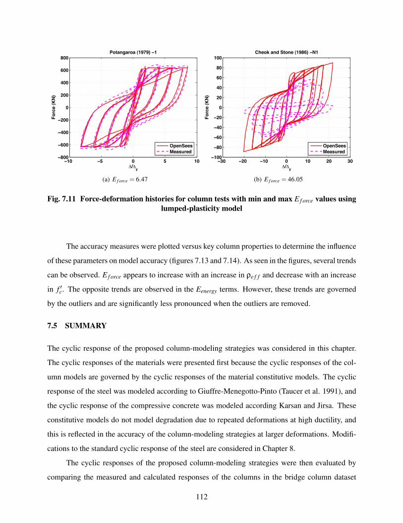
−10 −5 0 5 10−800
−600
−400
−200
0
200
400
600
800
∆/∆y
Fo
rce
(KN
)Potangaroa (1979) −1
OpenSeesMeasured
(a) E f orce = 6.47
−30 −20 −10 0 10 20 30−100
−80
−60
−40
−20
0
20
40
60
80
100
∆/∆y
Fo
rce
(KN
)
Cheok and Stone (1986) −N1
OpenSeesMeasured
(b) E f orce = 46.05
Fig. 7.11 Force-deformation histories for column tests with min and max E f orce values usinglumped-plasticity model
The accuracy measures were plotted versus key column properties to determine the influence
of these parameters on model accuracy (figures 7.13 and 7.14). As seen in the figures, several trends
can be observed. E f orce appears to increase with an increase in (e f f and decrease with an increase
in f ′c. The opposite trends are observed in the Eenergy terms. However, these trends are governed
by the outliers and are significantly less pronounced when the outliers are removed.
7.5 SUMMARY
The cyclic response of the proposed column-modeling strategies was considered in this chapter.
The cyclic responses of the materials were presented first because the cyclic responses of the col-
umn models are governed by the cyclic responses of the material constitutive models. The cyclic
response of the steel was modeled according to Giuffre-Menegotto-Pinto (Taucer et al. 1991), and
the cyclic response of the compressive concrete was modeled according Karsan and Jirsa. These
constitutive models do not model degradation due to repeated deformations at high ductility, and
this is reflected in the accuracy of the column-modeling strategies at larger deformations. Modifi-
cations to the standard cyclic response of the steel are considered in Chapter 8.
The cyclic responses of the proposed column-modeling strategies were then evaluated by
comparing the measured and calculated responses of the columns in the bridge column dataset
112

0 5 10 15 20 250
0.1
0.2
0.3
0.4
0.5
∆max
/ ∆y
Efo
rce
R2 = 0.33
0 5 10 15 20 25−1.5
−1
−0.5
0
0.5
∆max
/ ∆y
Een
erg
y
R2 = 0.23
Fig. 7.12 Effect of maximum ductility on cyclic accuracy for lumped-plasticity model
(Section 1.3). Similar accuracy can be obtained using either of the distributed-plasticity or lumped-
plasticity column-modeling strategies with standard cyclic material models. The mean values of
the force errors (E f orce) were 16.1% and 15.7% for the distributed-plasticity and lumped-plasticity
models, respectively. The mean values of the energy errors (Eenergy) were -23.7% and -19.9% for
the distributed-plasticity and lumped-plasticity models, respectively.
113

0 2 4 6 8 100
10
20
30
40
50
L/D
Efo
rce (
%)
R2 = 0.013
0 0.01 0.02 0.03 0.040
10
20
30
40
50
ρl
Efo
rce (
%)
R2 = 0.02
0 0.1 0.2 0.3 0.40
10
20
30
40
50
P/fcA
g
Efo
rce (
%)
R2 = 0.0016
0.05 0.1 0.15 0.2 0.25 0.30
10
20
30
40
50
ρeff
Efo
rce (
%)
R2 = 0.31
20 25 30 35 40 45−20
0
20
40
60
fc
Efo
rce (
%)
R2 = 0.36
1 2 3 4 50
10
20
30
40
50
S/db
Efo
rce (
%)
R2 = 0.1
Fig. 7.13 Effect of key column properties on E f orce using lumped-plasticity model
114

0 2 4 6 8 10−150
−100
−50
0
50
L/D
Een
erg
y (%
)
R2 = 0.012
0 0.01 0.02 0.03 0.04−150
−100
−50
0
50
ρl
Een
erg
y (%
)
R2 = 0.016
0 0.1 0.2 0.3 0.4−150
−100
−50
0
50
P/fcA
g
Een
erg
y (%
)
R2 = 0.003
0.05 0.1 0.15 0.2 0.25 0.3−150
−100
−50
0
50
ρeff
Een
erg
y (%
)R2 = 0.17
20 25 30 35 40 45−150
−100
−50
0
50
fc
Een
erg
y (%
)
R2 = 0.19
1 2 3 4 5−150
−100
−50
0
50
S/db
Een
erg
y (%
)
R2 = 0.074
Fig. 7.14 Effect of key column properties on Eenergy using lumped-plasticity model
115

8 Improved Cyclic Material Models
The cyclic responses of the fiber-model column-modeling strategies developed in this report de-
pend on the cyclic responses of the material models. The proposed modeling strategies with stan-
dard cyclic material models (Karsan and Jirsa concrete, and Giuffre-Menegotto-Pinto steel) were
evaluated in Chapter 7, and insufficiencies were identified. The cyclic response of the Giuffre-
Menegotto-Pinto steel does not model degradation due to bar fracture and cycling, while the Karsan
and Jirsa concrete model does not model imperfect crack closure.
In this chapter, a new steel model proposed by Mohle and Kunnath (2006) will be calibrated
and evaluated. The Karsan and Jirsa concrete model will be modified to model imperfect crack
closure, and a parametric study will be carried out to demonstrate the effects of this modification.
8.1 CALIBRATION OF MOHLE AND KUNNATH (2006) STEEL MODEL
To enhance the calculated cyclic response of the proposed modeling strategies, a more complex
steel constitutive model that accounts for cyclic degradation (Mohle and Kunnath 2006) was im-
plemented. In this section, the cyclic response of the Mohle and Kunnath (2006) steel model is
demonstrated, and key cyclic modeling parameters are identified and calibrated. The response of
the Mohle and Kunnath (2006) model depends on the calculated plastic-strain history of the bar,
and the strains calculated with the distributed-plasticity strategy are inaccurate in columns with
perfectly-plastic or degrading section behavior (Section 3.1.1). Therefore, the calibration and eval-
uation of this model was only carried out using the lumped-plasticity modeling strategy.
117

8.1.1 Cyclic Response of Model
The Mohle and Kunnath (2006) steel constitutive model is based on the steel model proposed by
Chang and Mander (1994). The model can be used to account for isotropic hardening, diminishing
yield plateau, the Bauschinger effect, degrading strength and stiffness due to bar buckling, and
degrading strength and stiffness due to cycling. Within the model, bar buckling can be modeled
according to models proposed by Dhakal and Maekawa (2002), or Gomes and Appleton (1997).
The degradation of strength and stiffness due to cycling was calculated according to the Coffin and
Manson fatigue model.
Because of numerical errors in the current implementation of the steel model in OpenSees
(v.1.7.0), the isotropic hardening component and bar-buckling components were neglected. How-
ever, the Bauschinger effect and the degradation of the steel due to cycling were modeled. The
Bauschinger effect was modeled using the model parameters suggested by Mohle and Kunnath
(2006).
The Mohle and Kunnath (2006) steel model uses a cyclic fatigue model proposed by Coffin
and Manson to model the effects of cycling on bar fracture. According to the Coffin and Manson
theory, a bar is assumed to fracture when the damage factor D reaches a value of 1.0. The damage
factor D is defined below.
D = -(
'p
Cf
) 1%
(8.1)
where: the half-cycle plastic-strain is defined as
'p = 't −)t
E(8.2)
't and )t are the total change in half-cycle strain and stress as illustrated in Figure 8.1(a). Cf and %
are factors used to relate the number of half cycles till fracture to 'p. This relationship is illustrated
in Figure 8.1(b).
In addition to fracture fatigue, the Mohle and Kunnath (2006) model accounts for loss in
strength due to cumulative damage. This degradation is controlled by the degradation parameter,
!SR, as illustrated in Figure 8.1(c). This parameter is defined in the following equation, where Cd
118

σ
εs
εt
σt
(a) Half Cycle Terms (b) Coffin-Manson Constants
σ
εs
DamageNo Damage
φSRσ
(c) Strength Reduction Factor
Fig. 8.1 Coffin and Manson parameters (based on Mohle and Kunnath, 2006)
is a factor that is calibrated with experimental results.
!SR = -(
'p
Cd
) 1%
(8.3)
The key modeling parameters identified in the previous discussion are presented below, and
the effects of these parameters are demonstrated in Figure 8.2.
Damage Strain Range Constant, % is used to relate damage from one strain range to an equiv-
alent damage at another strain range. This parameter is obtained from the calibration with
material tests, and is usually constant for a material type. For this research the value proposed
by Mohle and Kunnath (2006) is used, % = 0.506.
Ductility Constant, Cf adjusts the number of cycles to bar failure. The effect of this parameter
119

−0.06 −0.04 −0.02 0 0.02 0.04 0.06−2
−1.5
−1
−0.5
0
0.5
1
1.5σ/f y
εs
Cf = 1
Cd = 1
(a) Lesser Degradation, No Bar Failure
−0.06 −0.04 −0.02 0 0.02 0.04 0.06−1.5
−1
−0.5
0
0.5
1
1.5
σ/f y
εs
Cf = 1
Cd = 0.3
(b) More Degradation, No Bar Failure
−0.06 −0.04 −0.02 0 0.02 0.04 0.06−2
−1.5
−1
−0.5
0
0.5
1
1.5
σ/f y
εs
Cf = 0.2
Cd = 1
(c) Lesser Degradation, Bar Failure
−0.06 −0.04 −0.02 0 0.02 0.04 0.06−1.5
−1
−0.5
0
0.5
1
1.5
σ/f y
εs
Cf = 0.2
Cd = 0.3
(d) More Degradation, Bar Failure
Fig. 8.2 Effect of Coffin and Manson parameters on cyclic response of steel
is demonstrated by comparing figures 8.2(a) with 8.2(c), and 8.2(b) with 8.2(d). A higher
value for Cf results in a larger number of cycles to failure.
Strength Reduction Constant, Cd controls the amount of degradation per cycle. The effect of
this parameter is demonstrated by comparing figures 8.2(a) with 8.2(b), and 8.2(c) with
8.2(d). A higher Cd value will result in a lower reduction of strength for each cycle.
8.1.2 Optimization Strategy and Results
The Mohle and Kunnath (2006) steel model assumes that bar fracture occurs when the damage
index, D (Equation 8.1) reaches a value of 1.0. The bar-fracture component of the Mohle and
120

Kunnath (2006) steel model was calibrated with a subset of 20 columns from the bridge column
dataset in which bar fractures were reported. Cf was calibrated with this dataset by (1) calculating
the cyclic force-deformation responses of the 20 columns in the dataset for Cd = . and a given Cf
value, (2) calculating the mean value of the damage indices at the observed displacements at the
onset of bar fracture, (3) adjusting Cf accordingly and repeating procedure until the mean value of
the damage indices at the onset of bar fracture is 1.0. This procedure resulted in an optimal value
of Cf = 0.255. This value is nearly identical to the value recommended by Mohle and Kunnath
(2006), Cf = 0.26.
The strength reduction constant (Cd) was calibrated with the 37 column tests in the bridge
column dataset by minimizing the mean value of the force error term E f orce with Cf = 0.26. This
procedure resulted in an optimal value of Cd = 0.45.
Key accuracy statistics of the lumped-plasticity modeling strategy with the optimized Mohle
and Kunnath (2006) model, are provided in Table 8.1 for the 8 column tests performed by Lehman
and Moehle (2000), and for the 37 bridge columns. For illustration, the measured and calculated
cyclic force-deformation responses of the 8 columns are shown in Figure 8.3. The accuracy of the
lumped-plasticity column-modeling strategy using the Mohle and Kunnath (2006) steel model is
compared to the accuracy using the standard steel model in the summary of this chapter (Section
8.3).
Table 8.1 Cyclic response statistics (Kunnath steel with lumped-plasticity model)
Lehman Subset Bridge ColumnsE f orce abs(Eenergy) Eenergy E f orce abs(Eenergy) Eenergy
mean (%) 11.06 14.75 -7.42 11.98 12.88 -9.34min (%) 7.37 0.32 -33.84 5.15 0.14 -69.68max (%) 16.24 33.84 24.75 29.45 69.68 24.75
121

−15 −10 −5 0 5 10 15−600
−400
−200
0
200
400
600
∆/∆y
Fo
rce
(KN
)
Lehman & Calderone No.328
OpenSeesMeasured
−10 −5 0 5 10−200
−150
−100
−50
0
50
100
150
200
∆/∆y
Fo
rce
(KN
)
Lehman No.407
OpenSeesMeasured
−15 −10 −5 0 5 10 15−300
−200
−100
0
100
200
300
∆/∆y
Fo
rce
(KN
)
Lehman No.415
OpenSeesMeasured
−15 −10 −5 0 5 10 15−500
0
500
∆/∆y
Fo
rce
(KN
)
Lehman No.430
OpenSeesMeasured
−8 −6 −4 −2 0 2 4 6 8−150
−100
−50
0
50
100
150
200
∆/∆y
Fo
rce
(KN
)
Lehman No.815
OpenSeesMeasured
−15 −10 −5 0 5 10−300
−200
−100
0
100
200
300
∆/∆y
Fo
rce
(KN
)
Lehman & Calderone No.828
OpenSeesMeasured
−10 −5 0 5 10−150
−100
−50
0
50
100
150
∆/∆y
Fo
rce
(KN
)
Lehman No.1015
OpenSeesMeasured
−10 −5 0 5 10−200
−150
−100
−50
0
50
100
150
200
∆/∆y
Fo
rce
(KN
)
Lehman & Calderone No.1028
OpenSeesMeasured
Fig. 8.3 Force-deformation response, Kunnath steel model
122

8.2 IMPERFECT CRACK CLOSURE
Tension cracks in concrete can become partially filled with small particles of concrete sediments
and shear deformations in the column may result in misaligned cracks, causing some load to be
transferred across the cracks before they fully close. The standard concrete model developed as
part of this project (Popovic’s curve with Mander constants, and Karsan and Jirsa cyclic properties)
does not account for this phenomenon. The standard concrete model was modified to account for
this increase in strength and stiffness. The component of the model that accounts for the early
increase in strength is based on the model proposed by Stanton (1979).
8.2.1 Modified Concrete Model
The stress-strain response of the modified concrete model is illustrated in Figure 8.4, along with
the strain history used for the demonstration, and the resulting stiffness history. This response is
defined by the following rules.
1. The cyclic stress-strain curves in compression are contained within an envelope defined by
the Popovic’s curve. The concrete is assumed to have tension strength with exponentially
decreasing strength beyond ultimate tensile stress. This envelope response is described in
Section 2.2.2.
2. The unloading and reloading response of the concrete in tension is not modified from the
standard implementation. This response is defined in Section 7.1.
3. The unloading and reloading response of the concrete in compression is governed by stiff-
nesses Eu and Er, and strains '1, '2, '3, and '4. Each of these is illustrated in Figure 8.4(a),
and described below.
· Eu is the unloading stiffness defined by the Karsan and Jirsa concrete model.
· Er is the reloading stiffness. This value is calculated such that reloading follows a
straight line from the reloading strain to ('1, f1). This stiffness can be calculated as
follows.
Er =f1
'1− '4(8.4)
123

· '1 and f1 are the strain and stress at which the unloading curve departs from the enve-
lope curve.
· '2 is the strain at which the stress becomes zero.
· '3 is the maximum strain reached during the unload-reload cycle.
· '4 is the strain at which reloading starts.
Opening and closing of cracks both occur at zero stress. When strains exceed '2, cracks are
assumed to open. With perfect crack closure, they would close again when the strain returned
to '2. However, with imperfect crack closure, compression would begin to be transmitted at
a lower strain, '4. This reloading stress is calculated as follows.
'4 = '2 + r('3− '2) (8.5)
where: r is the proportion of the crack filled by sediment, 0≤ r ≤ 1.0, ('3− '2)≤ cmax, and
'3 ≤ 0.0.
If reloading stops before reaching the envelope (Figure 8.4(a), point F), unloading occurs at
a stiffness equal to the latest value of Eu. If unloading stops before the stress has reached
zero (point G), then reloading follows a straight line from the reversal point to ('1, f1).
The modeling parameters that can be varied to influence the reloading response of the con-
crete are r and cmax. The effect of varying r is illustrated in Figure 8.6. In this figure r is varied
from 0.0 to 1.0, while cmax is held constant. A value of r = 0.0 assumes perfect crack closure and
results in a model identical to the model described in Section 7.1. An increase in r assumes that
cracks will begin closing sooner upon reversal. The crack is assumed to close immediately upon
reversal when r = 1.0. Similarly, the effects of cmax are demonstrated in Figure 8.7. A value of
cmax = 0.0 also assumes perfect crack closure.
124

−7 −6 −5 −4 −3 −2 −1 0
x 10−3
−1
−0.8
−0.6
−0.4
−0.2
0
0.2σ
/f c,
εc
r = 0.75c
max = 0.0050
A
B
C
DE
F
G
H
ε2
ε3ε
4
Er
Eu
Eu
(ε1, f
1)
(a) Stress-strain response of concrete with imperfect crack Closure
0 100 200 300 400−7
−6
−5
−4
−3
−2
−1
0x 10
−3
A
B
C
DE
F
G
H
datapoint
ε c
(b) Strain history for response
0 100 200 300 400−0.4
−0.2
0
0.2
0.4
0.6
0.8
1A
B
C D
EF
G
H
datapoint
Tan
gen
t / E
c
(c) Tangent history of response
Fig. 8.4 Cyclic response of concrete with imperfect crack closure
125

0 100 200 300 400−7
−6
−5
−4
−3
−2
−1
0x 10
−3
datapoint
ε c
Fig. 8.5 Strain history for demonstration of imperfect crack closure properties
−7 −6 −5 −4 −3 −2 −1 0
x 10−3
−1
−0.8
−0.6
−0.4
−0.2
0
0.2
σ/f c,
εc
r = 0.00c
max = 0.0050
−7 −6 −5 −4 −3 −2 −1 0
x 10−3
−1
−0.8
−0.6
−0.4
−0.2
0
0.2σ
/f c,
εc
r = 0.33c
max = 0.0050
−7 −6 −5 −4 −3 −2 −1 0
x 10−3
−1
−0.8
−0.6
−0.4
−0.2
0
0.2
σ/f c,
εc
r = 0.67c
max = 0.0050
−7 −6 −5 −4 −3 −2 −1 0
x 10−3
−1
−0.8
−0.6
−0.4
−0.2
0
0.2
σ/f c,
εc
r = 1.00c
max = 0.0050
Fig. 8.6 Effect r on concrete stress-strain response
126

−7 −6 −5 −4 −3 −2 −1 0
x 10−3
−1
−0.8
−0.6
−0.4
−0.2
0
0.2σ
/f c,
εc
r = 1.00c
max = 0.0000
−7 −6 −5 −4 −3 −2 −1 0
x 10−3
−1
−0.8
−0.6
−0.4
−0.2
0
0.2
σ/f c,
εc
r = 1.00c
max = 0.0007
−7 −6 −5 −4 −3 −2 −1 0
x 10−3
−1
−0.8
−0.6
−0.4
−0.2
0
0.2
σ/f c,
εc
r = 1.00c
max = 0.0013
−7 −6 −5 −4 −3 −2 −1 0
x 10−3
−1
−0.8
−0.6
−0.4
−0.2
0
0.2
σ/f c,
εc
r = 1.00c
max = 0.0020
Fig. 8.7 Effect effect cmax on concrete stress-strain response
8.2.2 Parametric Study of Imperfect Crack Closure Parameters
For this project, a parametric study was carried out to demonstrate the effects of r and cmax on
model accuracy. For this study, the lumped-plasticity column-modeling strategy was used with the
Mohle and Kunnath (2006) steel to model the 8 column tests performed by Lehman and Moehle
(2000). The modified concrete model was used, and the parameters r and cmax were systematically
varied to demonstrate their influence. The effect of r is demonstrated in Figure 8.8. For this
analyses cmax was set to 0.005. In this figure, the mean values of E f orce and Eenergy are plotted
versus multiple values of r. As seen in this figure, r does not significantly affect E f orce. In contrast,
r does seem to affect Eenergy. As r increases, Eenergy gets further away from 0.0. At r = 1.0, Eenergy
is nearly 15% smaller (i.e., less accurate) than when r = 0.0.
127

In a similar fashion, the mean values of E f orce and Eenergy are plotted versus cmax. For this
analysis r = 0.5. The parameter cmax does not significantly influence E f orce; however it slightly
affects Eenergy. As cmax increases from 0.0 to 0.005, Eenergy decreases by 15%.
0 0.1 0.2 0.3 0.4 0.5 0.6 0.7 0.8 0.9 111.96
11.98
12
12.02
Efo
rce (
%)
r
0 0.1 0.2 0.3 0.4 0.5 0.6 0.7 0.8 0.9 1−11
−10
−9
Een
erg
y (%
)
r
Fig. 8.8 Effect of r on overall model accuracy (lumped-plasticity, Kunnath steel)
This study indicates that imperfect crack closure does not have a significant effect on the
accuracy of pseudo-static reinforced concrete column models. However, this phenomenon may
affect the calculated dynamic response of columns more significantly. This will be studied further
in a later chapter (Chapter 10).
8.3 SUMMARY
The cyclic modeling inaccuracies identified in Chapter 7 were addressed in this chapter. A steel
material model proposed by Mohle and Kunnath (2006), which accounts for degradation due to
cycling, was presented, calibrated, and evaluated. The use of this more complex steel constitutive
model improved the accuracy of the lumped-plasticity column-modeling strategy. The mean force
error (E f orce) decreased from 15.7% with the standard steel model to 12.6% with the Mohle and
Kunnath (2006) steel model and calibrated parameters (Cf = 0.26 and Cd = 0.45). The mean
energy error (Eenergy) was improved from -19.9% to -4.5%.
128

0 0.5 1 1.5 2 2.5 3 3.5 4 4.5 5
x 10−3
11.97
11.98
11.99
Efo
rce (
%)
cmax
0 0.5 1 1.5 2 2.5 3 3.5 4 4.5 5
x 10−3
−10.5
−10
−9.5
−9
Een
erg
y (%
)
cmax
Fig. 8.9 Effect of cmax on overall model accuracy (lumped-plasticity, Kunnath steel)
A concrete model that accounts for imperfect crack closure was also developed and evalu-
ated. The modifications to the standard Karsan and Jirsa cyclic material behavior to account for
imperfect crack closure did not significantly affect the accuracy of the lumped-plasticity modeling
strategy. It is possible that these modifications will affect the calculated residual displacements for
shake-table tests (Chapter 10).
129

9 Column Flexural Damage
To implement performance-based earthquake engineering for reinforced concrete bridges, it is
necessary to accurately predict column damage and assess the probability of reaching particular
levels of damage. This chapter develops and evaluates several methods that correlate engineering
demand parameters to damage measures. The engineering demand parameters considered in this
chapter are drift ratio, plastic rotation, and longitudinal strain.
The damage measures considered in this report are cover spalling, longitudinal bar buckling,
and longitudinal bar fracture. This report considered concrete cover spalling (Figure 9.1(a)) be-
cause it represents the first flexural damage state in which there are marginal safety implications,
there may be a possible short-term loss of function, and the cost to repair concrete spalling could be
significant. Buckling and fracture of the longitudinal bars (Figure 9.1(b)) were also considered be-
cause these levels of damage represent damage states in which safety implications are significant,
partial replacement may be required, and a longer-term loss of function may occur.
9.1 ESTIMATES BASED ON DRIFT RATIO
Berry and Eberhard (2003) developed empirical equations to estimate deformations at bar buckling
and cover concrete spalling based on theoretically expected trends in drift ratios, displacement
ductilities, plastic rotations, and longitudinal strains. Because the drift-ratio equations are the
simplest to use (e.g., no estimate of yield displacement), and because these equations were as
accurate as the more complex methods, the drift-ratio equations were chosen as the most suitable
for many practical situations. The bar-buckling equations were modified in Berry and Eberhard
(2005). The resulting equations for the drift ratio at the onset of cover spalling ("spallL ) and bar
131

(a) Spalling of cover concrete (b) Longitudinal bar buckling
(c) Longitudinal bar fracture
Fig. 9.1 Key flexural damage states (Ranf, 2006)
buckling ("bbL ) are provided below.
"calcsp
L(%)∼= 1.6
(1− P
Ag f ′c
) (1+
L10D
)(9.1)
"calcbbL
(%) = 3.25(
1+ ke(e f fdb
D
)(1− P
Ag f ′c
) (1+
L10D
)(9.2)
where ke = 40 for rectangular columns and 150 for spiral-reinforced columns, (e f f = (sfysf ′c
, (s is
the volumetric transverse reinforcement ratio, fys is the yield stress of the transverse reinforcement,
f ′c is the concrete compressive strength, db is the diameter of the longitudinal reinforcement, D is
the column depth, P is the axial load, Ag is the gross area of the cross section, and L is the distance
132

from the column base to the point of contraflexure.
The dataset originally used in the calibration of the spalling equation contained 102 rectangular-
reinforced columns and 40 spiral-reinforced columns. The ratios of the measured displacements at
cover spalling to the displacements calculated with the proposed model (Equation 9.1) had a mean
of 0.97 for rectangular columns with a c.o.v. of 43%, and a mean of 1.07 with a c.o.v. 35% for
spiral-reinforced columns (Berry and Eberhard 2003).
The dataset originally used in the calibration of the buckling equation contained 62 rectangular-
reinforced columns and 42 spiral-reinforced columns. The ratios of the measured displacements at
bar buckling to the displacements calculated with the proposed model (Equation 9.2) had a mean
of 1.01 and a coefficient of variation of 25% for rectangular-reinforced concrete columns. The
corresponding mean and coefficient of variation for spiral-reinforced columns were 0.97 and 24%,
respectively (Berry and Eberhard 2005).
The bridge column dataset used in this report is a subset of the dataset originally used to
calibrate the drift-ratio equations described above. The accuracy statistics of the drift-ratio equa-
tions (9.1 and 9.2) applied to the bridge column dataset used in this report (29 observations of
cover spalling and 33 observations of bar buckling) are presented in Table 9.1. In this table and
throughout this chapter, the subscript dam is used to indicate a general damage state. For exam-
ple, "measdam would be "meas
sp for the cover-spalling damage state. For the bridge dataset, the ratios
Table 9.1 Key accuracy statistics of drift-ratio equations with bridge column dataset
Statistics of "measdam /L% Statistics of "meas
dam /"calcdam
Dataset Damage State min max mean cov (%) min max mean cov (%)
Original Dataset Cover Spalling 0.61 4.51 2.30 44.2 0.48 1.75 1.07 34.9Bar Buckling 2.31 14.62 6.59 43.2 0.46 1.62 0.97 24.0
Bridge ColumnsCover Spalling 0.75 4.17 2.34 38.9 0.48 1.75 1.07 34.9Bar Buckling 3.75 14.58 7.39 37.1 0.64 1.62 1.01 24.7Bar Fracture 3.75 12.30 7.63 25.9 0.60 1.48 0.97 20.0
of the measured displacements at cover spalling to the displacements calculated with the proposed
model (Equation 9.1) have a mean of 1.07 and a coefficient of variation of 35%. The corresponding
mean and coefficient of variation for bar buckling is 1.01 and 25%, respectively. The accuracy of
equations 9.1 and 9.2 are nearly identical when applied to the smaller bridge column dataset.
As part of this project, an equation was developed to predict the drift ratio at the onset of
133

bar buckling by recalibrating the coefficients of Equation 9.2 with the bridge column subset. The
resulting equation is as follows.
"calcb f
L(%) = 3.5
(1+150(e f f
db
D
)(1− P
Ag f ′c
) (1+
L10D
)(9.3)
The coefficient of variation of the ratios of measured to calculated (from Equation 9.3) displace-
ments at the onset of bar fracture was 20.0% (Table 9.1).
Fragility curves are helpful in the design and assessment in performance-based earthquake
engineering. Fragility curves help a designer answer the following question:
For a particular level of column deformation, what is the likelihood that the longitudi-
nal reinforcement will have begun to buckle?
Figure 9.2 shows the fragility curves for cover spalling, bar buckling, and bar fracture in spiral-
reinforced columns for the dataset used in this project. In these figures, the Y-axis is the cumulative
probability of cover spalling or bar buckling, and the X-axis is the ratio of "measdam
"calcdam
. If the database is
assumed to be representative of the entire population of spiral-reinforced columns, this ratio can be
interpreted as "demanddam"calc
dam. These plots also show the normal cumulative distribution functions (CDF)
and the lognormal cumulative distribution functions.
In some situations, the normal CDF may fit the data better than the lognormal CDF. However,
the normal CDF allows negative values of "demanddam /"calc
dam at low probabilities.
The ratios of measured to calculated displacements at the onset of cover spalling, bar buck-
ling, and bar fracture are plotted versus key column properties in figures 9.3 and 9.5 to evaluate
the effect of these properties on the accuracy of the proposed equations. As seen in Figure 9.3, the
ratios of measured to calculated displacements increase with an increase in effective confinement
ratio and decrease with an increase in concrete compressive strength. The effect of confinement
on cover spalling is addressed later in this chapter. With respect to bar buckling (Figure 9.4),
the ratios increase slightly with an increase in aspect ratio, longitudinal-reinforcement ratio, and
concrete compressive strength. No significant trends are observed in the bar-fracture ratios.
134

0 0.5 1 1.5 20
0.2
0.4
0.6
0.8
1
∆spallmeas / ∆
spallcalc
Pro
bab
ility
of
Co
ver
Sp
allin
g
Normal CDFLognormal CDF
0 0.5 1 1.5 20
0.2
0.4
0.6
0.8
1
∆bbmeas / ∆
bbcalc
Pro
bab
ility
of
Bar
Bu
cklin
g
Normal CDFLognormal CDF
0 0.5 1 1.5 20
0.2
0.4
0.6
0.8
1
∆bfmeas / ∆
bfcalc
Pro
bab
ility
of
Bar
Fra
ctu
re
Normal CDFLognormal CDF
Fig. 9.2 Fragility curves for cover spalling, bar buckling, and bar fracture using drift-ratioequations
135

0 5 100
0.5
1
1.5
2
L/D
∆spm
eas /
∆spca
lc
R2 = 0.032
0 0.01 0.02 0.030
0.5
1
1.5
2
ρl
∆spm
eas /
∆spca
lc
R2 = 0.035
0 0.05 0.1 0.15 0.20
0.5
1
1.5
2
P/fcA
g
∆spm
eas /
∆spca
lc
R2 = 0.02
0 0.1 0.2 0.30
0.5
1
1.5
2
ρeff
∆spm
eas /
∆spca
lcR2 = 0.32
0 10 20 30 400
0.5
1
1.5
2
fc
∆spm
eas /
∆spca
lc
R2 = 0.17
0 1 2 3 40
0.5
1
1.5
2
S/db
∆spm
eas /
∆spca
lc
R2 = 0.035
Fig. 9.3 Effect of key column properties on accuracy of drift-ratio cover-spalling equations
136

0 5 100
0.5
1
1.5
2
L/D
∆b
bm
eas /
∆b
bca
lc
R2 = 0.16
0 0.01 0.02 0.03 0.040
0.5
1
1.5
2
ρl
∆b
bm
eas /
∆b
bca
lc
R2 = 0.12
0 0.1 0.2 0.3 0.40
0.5
1
1.5
2
P/fcA
g
∆b
bm
eas /
∆b
bca
lc
R2 = 0.0018
0 0.1 0.2 0.3 0.40
0.5
1
1.5
2
ρeff
∆b
bm
eas /
∆b
bca
lcR2 = 1.1e−005
0 10 20 30 40 500
0.5
1
1.5
2
fc
∆b
bm
eas /
∆b
bca
lc
R2 = 0.11
0 1 2 3 4 50
0.5
1
1.5
2
S/db
∆b
bm
eas /
∆b
bca
lc
R2 = 0.074
Fig. 9.4 Effect of key column properties on accuracy of drift-ratio bar-buckling equations
137

0 5 100
1
2
L/D
∆b
fm
eas /
∆b
fca
lc
R2 = 0.0057
0 0.01 0.02 0.03 0.040
1
2
ρl
∆b
fm
eas /
∆b
fca
lc
R2 = 0.089
0 0.1 0.2 0.3 0.40
1
2
P/fcA
g
∆b
fm
eas /
∆b
fca
lc
R2 = 0.00044
0 0.1 0.2 0.3 0.40
1
2
ρeff
∆b
fm
eas /
∆b
fca
lc
R2 = 0.048
0 10 20 30 40 500
1
2
fc
∆b
fm
eas /
∆b
fca
lc
R2 = 0.049
0 1 2 3 4 50
1
2
S/db
∆b
fm
eas /
∆b
fca
lc
R2 = 0.058
Fig. 9.5 Effect of key column properties on accuracy of drift-ratio bar-fracture equations
138

The drift-ratio equations provide a practical correlation between an engineering demand pa-
rameter and key damage states. However, the drift-ratio equations may not always be applicable,
such as cases in which the distance to the point of contraflexure is unknown or varies. Therefore,
similar damage estimates will be developed for other, more versatile engineering damage parame-
ters: plastic rotations and longitudinal strain.
9.2 DAMAGE ESTIMATES BASED ON PLASTIC ROTATION
Empirical equations, similar to the drift-ratio equations, can be developed for the plastic rotation
at the onset of particular damage states. This engineering demand parameter may be more ver-
satile than drift ratio because plastic rotations can be calculated in a complex model more easily.
The plastic rotations calculated with the distributed-plasticity modeling strategy (with no bond slip
component) should be identical to the plastic rotations calculated with the lumped-plasticity for-
mulation if the plastic curvatures calculated from the distributed-plasticity strategy are adjusted to
account for localization in accordance to the method presented in Section 3.1.1. If the zero-length
bond-slip section is used in the distributed-plasticity modeling strategy, the rotation due to bond
slip must be added to the rotations recorded at the integration points, because these rotations will
be relative rotations, and the following equations were developed for total rotations.
Berry and Eberhard (2003) demonstrated that the plastic rotation at the onset of damage
(0calcp dam) should increase with an increase in aspect ratio (L/D) and key longitudinal-reinforcement
properties ( fydb/D), and decrease with an increase in axial-load ratio (P/Ag f ′c), as indicated in
Equation 9.4.
0calcp dam = C0 ('dam)
(1+C1
PAg f ′c
)−1 (1+C2
LD
+C3fydb
D
)(9.4)
where 'dam is the strain at the onset of cover spalling ('sp) or bar buckling ('bb), and C0−C3 are
constants to be calibrated with experimental results.
In the following subsections, Equation 9.4 will be calibrated for cover spalling, bar buckling,
and bar fracture. The corresponding equations were calibrated by obtaining values of C0−C3 such
that the coefficients of variation of the ratios of measured to calculated displacements at the onset
of the particular damage states ("measdam /"calc
dam) were minimized. The calculated displacements at the
onset of the damage states are the displacements associated with the calculated values of 0calcp dam
from Equation 9.4.
139

9.2.1 Cover Spalling
The observed plastic rotations at the onset of cover spalling, 0 measp sp , (calculated from the observed
displacements at cover spalling) have a mean value of 1.50% with a coefficient of variation of
49.7% (Table 9.2). The mean value of the ratios of the measured displacements to the calculated
displacements associated with the mean value of 0measp sp is 0.98 with a coefficient of variation of
33.9%.
This estimate of the plastic rotation at the onset of cover spalling can be improved by con-
sidering the trends proposed in Equation 9.4. For cover spalling, 'sp is not expected to vary with
the amount of traverse or longitudinal reinforcement; therefore the plastic rotation at the onset of
cover spalling can be approximated with the following simplified expression.
0calcp sp = C0
(1+C1
PAg f ′c
)−1 (1+C2
LD
+C3fydb
D
)(9.5)
This equation was calibrated with the method discussed previously. The resulting coefficients and
accuracy statistics are presented in Table 9.2. For comparison, the table includes the estimates
based on the displacements calculated with the mean value of the plastic rotation at the onset of
the particular damage states. This method is equivalent to setting C0 in Equation 9.5 to the mean
value of 0measp sp , and setting the other coefficients to zero.
Table 9.2 Results of plastic-rotation calibration
Coefficients 0measp sp /0calc
p sp "measdam /"calc
dam
Methodology C0 C1 C2 C3 C4 mean cov (%) mean cov (%)
mean 0p sp 0.015 - - - - 1.00 49.7 0.98 33.9Eq (9.5) 0.0095 0.001 0.08 0.015 - 0.99 48.1 0.99 33.3
Little accuracy is gained by utilizing the expected trends in plastic rotation at the onset of
cover spalling (Equation 9.5). The coefficient of variation of "meassp /"calc
sp with Equation 9.5 was
33.3%, which is only slightly more accurate than using the mean value of 0p sp (1.50%) to calculate
the displacement at the onset of cover spalling, "meansp (33.9%). Additionally, a slightly smaller co-
efficient of variation can be obtained using a constant plastic rotation of 1.20% (32.5%). Therefore,
this value recommended for calculating the plastic rotation at the onset of cover spalling.
Fragility curves for estimates of the plastic rotations at the onset of cover spalling are shown
140
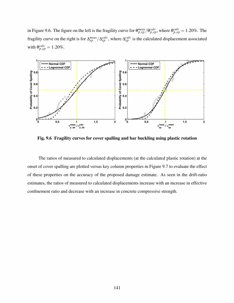
in Figure 9.6. The figure on the left is the fragility curve for 0measp sp /0calc
p sp, where 0calcp sp = 1.20%. The
fragility curve on the right is for "meassp /"calc
sp , where "calcsp is the calculated displacement associated
with 0calcp sp = 1.20%.
0 0.5 1 1.5 20
0.2
0.4
0.6
0.8
1
θp_bbmeas / θ
p_bbcalc
Pro
bab
ility
of
Co
ver
Sp
allin
g
Normal CDFLognormal CDF
0 0.5 1 1.5 20
0.2
0.4
0.6
0.8
1
∆spmeas / ∆
spmean
Pro
bab
ility
of
Co
ver
Sp
allin
g
Normal CDFLognormal CDF
Fig. 9.6 Fragility curves for cover spalling and bar buckling using plastic rotation
The ratios of measured to calculated displacements (at the calculated plastic rotation) at the
onset of cover spalling are plotted versus key column properties in Figure 9.7 to evaluate the effect
of these properties on the accuracy of the proposed damage estimate. As seen in the drift-ratio
estimates, the ratios of measured to calculated displacements increase with an increase in effective
confinement ratio and decrease with an increase in concrete compressive strength.
141

0 5 100
0.5
1
1.5
2
L/D
∆spm
eas /
∆spca
lc
R2 = 0.11
0 0.01 0.02 0.030
0.5
1
1.5
2
ρl
∆spm
eas /
∆spca
lc
R2 = 0.052
0 0.05 0.1 0.15 0.20
0.5
1
1.5
2
P/fcA
g
∆spm
eas /
∆spca
lc
R2 = 0.088
0 0.1 0.2 0.30
0.5
1
1.5
2
ρeff
∆spm
eas /
∆spca
lcR2 = 0.23
0 10 20 30 400
0.5
1
1.5
2
fc
∆spm
eas /
∆spca
lc
R2 = 0.12
0 1 2 3 40
0.5
1
1.5
2
S/db
∆spm
eas /
∆spca
lc
R2 = 0.039
Fig. 9.7 Effect of key column properties on accuracy of plastic-rotation cover-spallingequations
142

9.2.2 Bar Buckling
The mean value and coefficient of variation of the observed plastic rotations at the onset of bar
buckling (0 measp bb ) were 6.50% and 39.1%, respectively. The mean and coefficient of variation of the
ratios of measured displacements at the onset of bar buckling to the displacements associated with
the mean value of 0measp bb were 0.99 and 34.4%, respectively.
Estimates of the plastic rotation at the onset of bar buckling can be improved by considering
the trends proposed in Equation 9.4. The plastic-rotation equation can be extended further for bar
buckling by considering the effect of the confining steel on the strain at bar buckling. The strain
at the onset of bar buckling is expected to increase with an increase in effective confinement ratio
((e f f = (s fys/ f ′c) as in the following equation.
'bb = 21 +22(e f f (9.6)
By combining Equation 9.6 with Equation 9.4, simplifying, and combining constants, the
following equation for the plastic rotation at the onset of bar buckling is obtained.
0p bb = C0(1+C4(e f f
)(1+C1
PAg f ′c
)−1 (1+C2
LD
+C3fydb
D
)(9.7)
The coefficients in the bar-buckling equation (Equation 9.7) were previously calibrated by
Berry and Eberhard (2005). However the coefficients obtained in their study were developed for a
different model formulation and dataset. Therefore, the equations were recalibrated as part of this
study with the bridge column dataset and new model formulation.
The resulting coefficients and accuracy statistics are presented in Table 9.3. For comparison,
the table includes the estimates based on the displacements calculated with the mean value of 0measp bb .
This method is equivalent to setting C0 in equation 9.7 to the mean value of 0measp bb , and setting the
other coefficients to zero. The coefficients for Equation 9.7 previously calibrated by Berry and
Eberhard (2005) are also included in the table.
As seen in Table 9.3, Equation 9.7 provides an accurate means of estimating bar buckling.
The coefficient of variation of the ratios of measured to calculated displacements at the onset of
bar buckling was 21.1%. This is an improvement to the 25% coefficient of variation obtained using
143
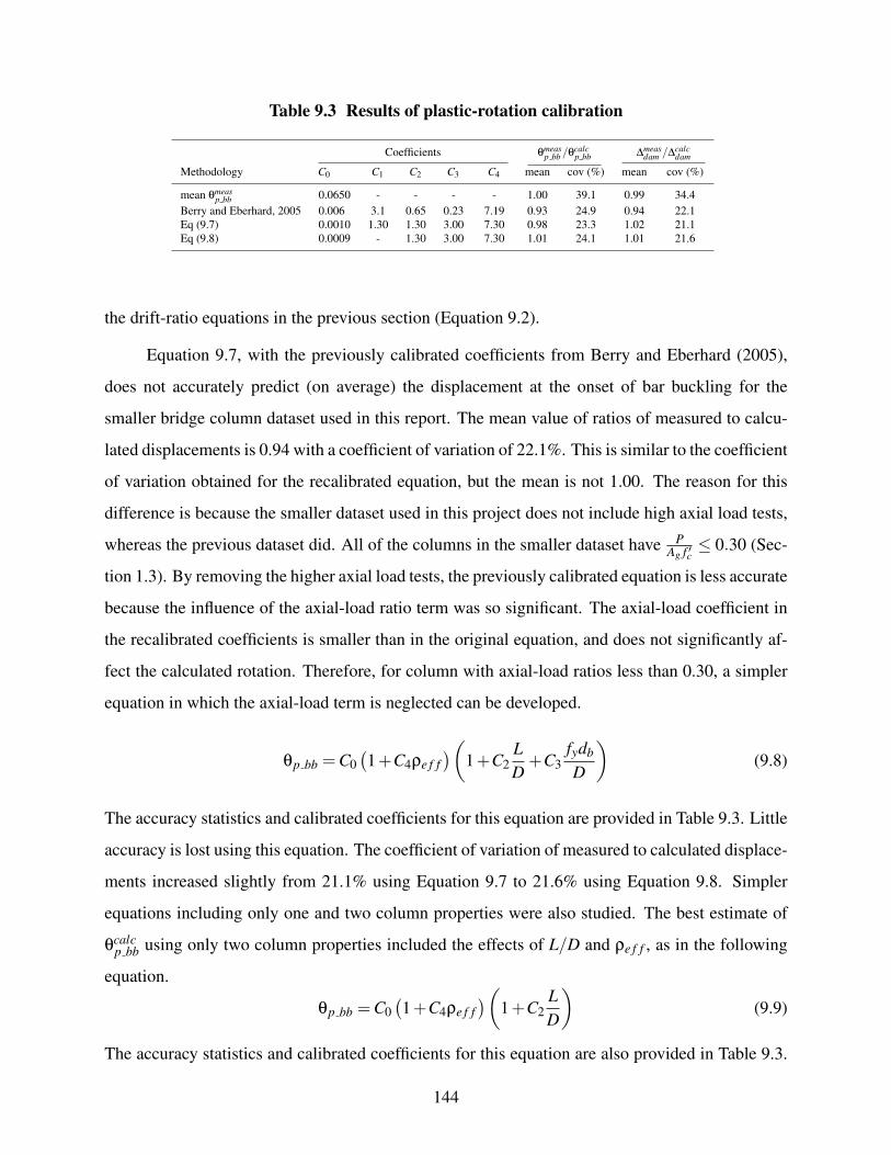
Table 9.3 Results of plastic-rotation calibration
Coefficients 0measp bb /0calc
p bb "measdam /"calc
dam
Methodology C0 C1 C2 C3 C4 mean cov (%) mean cov (%)
mean 0measp bb 0.0650 - - - - 1.00 39.1 0.99 34.4
Berry and Eberhard, 2005 0.006 3.1 0.65 0.23 7.19 0.93 24.9 0.94 22.1Eq (9.7) 0.0010 1.30 1.30 3.00 7.30 0.98 23.3 1.02 21.1Eq (9.8) 0.0009 - 1.30 3.00 7.30 1.01 24.1 1.01 21.6
the drift-ratio equations in the previous section (Equation 9.2).
Equation 9.7, with the previously calibrated coefficients from Berry and Eberhard (2005),
does not accurately predict (on average) the displacement at the onset of bar buckling for the
smaller bridge column dataset used in this report. The mean value of ratios of measured to calcu-
lated displacements is 0.94 with a coefficient of variation of 22.1%. This is similar to the coefficient
of variation obtained for the recalibrated equation, but the mean is not 1.00. The reason for this
difference is because the smaller dataset used in this project does not include high axial load tests,
whereas the previous dataset did. All of the columns in the smaller dataset have PAg f ′c
≤ 0.30 (Sec-
tion 1.3). By removing the higher axial load tests, the previously calibrated equation is less accurate
because the influence of the axial-load ratio term was so significant. The axial-load coefficient in
the recalibrated coefficients is smaller than in the original equation, and does not significantly af-
fect the calculated rotation. Therefore, for column with axial-load ratios less than 0.30, a simpler
equation in which the axial-load term is neglected can be developed.
0p bb = C0(1+C4(e f f
)(1+C2
LD
+C3fydb
D
)(9.8)
The accuracy statistics and calibrated coefficients for this equation are provided in Table 9.3. Little
accuracy is lost using this equation. The coefficient of variation of measured to calculated displace-
ments increased slightly from 21.1% using Equation 9.7 to 21.6% using Equation 9.8. Simpler
equations including only one and two column properties were also studied. The best estimate of
0calcp bb using only two column properties included the effects of L/D and (e f f , as in the following
equation.
0p bb = C0(1+C4(e f f
)(1+C2
LD
)(9.9)
The accuracy statistics and calibrated coefficients for this equation are also provided in Table 9.3.
144

As seen in the table, if only two column properties are used in the estimate, the accuracy of the
damage estimate is reduced. The coefficient of variation of the measured to calculated displace-
ments are reduced from 21.6% using Equation 9.8 to 27.3% using Equation 9.9.
The best one property estimate of 0calcp bb included the effects of the column aspect ratio (L/D)
as in the following equation.
0p bb = C0
(1+C2
LD
)(9.10)
The calibrated coefficients and accuracy statistics for this equation are also provided in Table 9.3.
In this case, the coefficient of variation of the ratios of measured to calculated displacements is
29.5%, significantly larger than the 21.6% using three column properties.
Equation 9.8 provides a practical compromise between simplicity and accuracy; this estimate
is simpler than Equation 9.7, and little accuracy is lost when using this simpler equation. However,
this equation was developed for columns with axial-load ratios less than 0.30. This should be
considered when applying this equation because previous research (Berry and Eberhard 2005)
indicates that axial load influences the plastic rotation at the onset of damage.
For comparison and simplicity, an equation was developed that has a similar form to the
simplified drift-ratio equations of the previous section (Equation 9.2). The resulting equation is as
follows.
0calcp bb(%) = 2.75
(1+150(e f f db/D
)(1−P/Ag f ′c
)(1+L/10D) (9.11)
Using this equation, the mean and coefficient of variation of the ratios of measured to calculated
plastic rotations were 1.01 with a coefficient of variation of 28.3%, whereas the mean and coeffi-
cient of variation of the ratios of measured displacements to calculated displacements associated
with the rotations calculated with Equation 9.12 were 1.01 with a coefficient of variation of 24.3%.
Fragility curves for estimates of the plastic rotations at the onset of bar buckling are shown
in Figure 9.8. The figure on the left is the fragility curve for 0measp bb /0calc
p bb, where 0calcp bb is calculated
with Equation 9.8 and coefficients in Table 9.3. The fragility curve on the right is for "measbb /"calc
bb ,
where "calcbb is the calculated displacement associated with 0calc
p bb.
145

0 0.5 1 1.5 20
0.2
0.4
0.6
0.8
1
θp_bbmeas / θ
p_bbcalc
Pro
bab
ility
of
Bar
Bu
cklin
gNormal CDFLognormal CDF
0 0.5 1 1.5 20
0.2
0.4
0.6
0.8
1
∆bbmeas / ∆
bbcalc
Pro
bab
ility
of
Bar
Bu
cklin
g
Normal CDFLognormal CDF
Fig. 9.8 Fragility curves for bar buckling using plastic rotation
The ratios of measured to calculated displacements (from the calculated plastic rotation) at
the onset of bar buckling are plotted versus key column properties in Figure 9.9 to evaluate the
effect of these properties on the accuracy of the proposed damage estimate. No significant trends
are observed in the data.
9.2.3 Bar Fracture
The plastic-rotation equations developed for the onset of bar buckling (equations 9.7 and 9.8) were
calibrated to estimate the onset of bar fracture. The results of this calibration are presented in Table
9.4.
Table 9.4 Results of plastic-rotation calibration
Coefficients 0measp b f /0calc
p b f "measdam /"calc
dam
Methodology C0 C1 C2 C3 C4 mean cov (%) mean cov (%)
mean 0p b f 0.0650 - - - - 1.00 39.1 0.99 34.4Eq (9.7) 0.0010 1.0 2.4 1.7 6.7 1.00 17.5 0.98 15.2Eq (9.8) 0.0009 - 2.4 1.7 6.7 0.99 18.3 0.99 16.0
146

0 5 100
0.5
1
1.5
2
L/D
∆b
bm
eas /
∆b
bca
lc R2 = 0.046
0 0.01 0.02 0.03 0.040
0.5
1
1.5
2
ρl
∆b
bm
eas /
∆b
bca
lc R2 = 0.053
0 0.1 0.2 0.3 0.40
0.5
1
1.5
2
P/fcA
g
∆b
bm
eas /
∆b
bca
lc R2 = 0.043
0 0.1 0.2 0.30
0.5
1
1.5
2
ρeff
∆b
bm
eas /
∆b
bca
lc R2 = 0.00016
0 10 20 30 400
0.5
1
1.5
2
fc
∆b
bm
eas /
∆b
bca
lc R2 = 0.11
0 1 2 3 4 50
0.5
1
1.5
2
S/db
∆b
bm
eas /
∆b
bca
lc R2 = 0.022
Fig. 9.9 Effect of key column properties on accuracy of plastic-rotation bar-bucklingequation
147

As seen in this table, estimates of plastic rotations at the onset of bar fracture are significantly
improved by considering the effects of the key column properties. The coefficient of variation of
measured to calculated displacements is reduced from 34.4% using the mean value of 0measp b f to
15.2% using Equation 9.7, and 16.0% using Equation 9.8. Little accuracy is gained by considering
the axial load term in the bar-fracture estimates. Therefore, Equation 9.8 is recommended for
columns with axial ratios ≤ 0.30.
A simplified equation similar to the equation developed for the drift ratio at the onset of bar
fracture (Equation 9.3) was developed for the plastic rotation as follows.
0calcp b f (%) = 3.0
(1+150(e f f db/D
)(1−P/Ag f ′c
)(1+L/10D) (9.12)
The mean value of the ratios of measured to calculated plastic rotations were 0.97 with a coefficient
of variation of 22.7%, whereas the corresponding mean and coefficient of variation for the ratios
of measured to calculated displacements were 0.97 and 19.6%.
Fragility curves for this damage state and engineering demand parameter are provided in
Figure 9.10, and the ratios of measured to calculated displacements are plotted versus key column
properties in Figure 9.11. The only significant trend observed in the data is a slight increase in the
ratios of measured to calculated displacements with an increase in concrete compressive strength.
9.3 DAMAGE ESTIMATES BASED ON STRAIN
Longitudinal strains introduce more information into the prediction process, and thus may provide
more versatile and accurate predictions of damage. Additionally, the empirical equations based on
drift ratio and plastic rotation developed in the previous sections may not be applicable to some
modeling situations, such as cases where the distance to the point of contraflexure varies, the axial
load varies, or there is biaxial bending. This section will focus on developing and evaluating
damage predictions based on longitudinal strain.
Tests show that the onset of cover spalling correlates to the maximum compressive strain
in the cover concrete (Lehman and Moehle 2000), therefore this parameter is chosen as the local
engineering demand parameter for this damage state. The tensile strain in the extreme reinforcing
bar was chosen as the local engineering demand parameter for longitudinal bar buckling; this
148

0 0.5 1 1.5 20
0.2
0.4
0.6
0.8
1
θp_bfmeas / θ
p_bfcalc
Pro
bab
ility
of
Bar
Bu
cklin
gNormal CDFLognormal CDF
0 0.5 1 1.5 20
0.2
0.4
0.6
0.8
1
∆bfmeas / ∆
bfcalc
Pro
bab
ility
of
Bar
Fra
ctu
re
Normal CDFLognormal CDF
Fig. 9.10 Fragility curves for bar fracture using plastic rotation
parameter is suggested by multiple researchers including Moyer and Kowalsky (2001), Priestley
et al. (1996), and Lehman and Moehle (2000). Tensile strain is chosen for bar fracture because bar
fracture often occurs immediately after buckling of the longitudinal reinforcement.
The lumped-plasticity modeling strategy developed in this report will be used to evaluate
the effectiveness of using maximum concrete compressive strain to estimate cover spalling, and
maximum longitudinal-reinforcement tensile strain to estimate bar buckling and bar fracture. Key
statistics and fragility curves will be presented. The calibration of the proposed plastic-hinge length
in this report considered the estimation of these damage states, and the reader is referred to Section
6.3 for details on this procedure.
The evaluation will not be carried out for both modeling strategies proposed in this report be-
cause the longitudinal strains calculated with the distributed-plasticity method are subject to strain
concentrations in columns with perfectly-plastic or degrading behavior, as indicated in Section
3.1.1. Strain estimates based on this methodology are only valid for columns with hardening re-
sponses, and all of the columns in the bridge dataset do not portray this type of response, whereas
the strains estimated with the lumped-plasticity formulation are objective for all section responses.
149

0 5 100
1
2
L/D
∆b
fm
eas /
∆b
fca
lc
R2 = 0.03
0 0.01 0.02 0.03 0.040
1
2
ρl
∆b
fm
eas /
∆b
fca
lc
R2 = 0.0051
0 0.1 0.2 0.3 0.40
1
2
P/fcA
g
∆b
fm
eas /
∆b
fca
lc
R2 = 0.081
0 0.1 0.2 0.3 0.40
1
2
ρeff
∆b
fm
eas /
∆b
fca
lc
R2 = 0.00034
0 10 20 30 40 500
1
2
fc
∆b
fm
eas /
∆b
fca
lc
R2 = 0.12
0 1 2 3 4 50
1
2
S/db
∆b
fm
eas /
∆b
fca
lc
R2 = 0.001
Fig. 9.11 Effect of key column properties on accuracy of plastic-rotation bar-fractureequation
150

9.3.1 Cover Spalling
The mean value of the compressive strains at the onset of cover spalling ('meassp ) was 0.008 with a
coefficient of variation of 48.6%. The mean value of the ratios of observed spalling displacements
to the displacement associated with the mean value of 'meassp was 0.99 with a coefficient of variation
of 34.7% (Table 9.5).
Table 9.5 Cover-spalling estimates based on longitudinal compressive strain
'meassp /'calc
sp "meassp /"calc
sp
Methodology mean cov (%) mean cov (%)
mean 'sp = 0.008 1.00 48.6 0.99 34.7Eq (9.13) 0.99 39.6 1.0 27.5
The strain at the onset of cover spalling is not expected to increase with an increase of effec-
tive confinement ratio. However, if 'sp is plotted versus (e f f , a significant trend can be observed
(Figure 9.12). The best fit line for this trend is as follows.
'calcsp = 0.0004+0.045(e f f (9.13)
The R2 value for this correlation is 0.42. The effective confinement ratio may be affecting the
compressive strain at the onset of cover spalling by confining the lateral expansion of the concrete
core and longitudinal reinforcement. If this trend is included in the estimate of the displacement at
the onset of cover spalling ("calcsp ), a significantly better estimate can be obtained. As seen in Table
9.5, the coefficient of variation of the ratios of measured to calculated displacements at the onset
of spalling can be reduced from 34.5% to 27.5%. This phenomenon requires a more thorough
investigation before this method is recommended for use.
Fragility curves for estimates of the compressive strain at the onset of cover spalling are
shown in Figure 9.13. The figure on the left is the fragility curve for 'meassp /'calc
sp , where 'calcsp is the
mean value of the observed strain 0.008. The fragility curve on the right is for "meassp /"calc
sp , where
"calcsp is the calculated displacement associated with the mean value of 'sp (0.008).
151

0 0.05 0.1 0.15 0.2 0.250
0.002
0.004
0.006
0.008
0.01
0.012
0.014
ρeff
ε sp
R2 = 0.42
Fig. 9.12 Effect of effective confinement ratio on 'sp
0 0.5 1 1.5 20
0.2
0.4
0.6
0.8
1
εspmeas / ε
spcalc
Pro
bab
ility
of
Co
ver
Sp
allin
g
Normal CDFLognormal CDF
0 0.5 1 1.5 20
0.2
0.4
0.6
0.8
1
∆spmeas / ∆
spmean
Pro
bab
ility
of
Co
ver
Sp
allin
g
Normal CDFLognormal CDF
Fig. 9.13 Fragility curves for cover spalling and bar buckling using longitudinal strain
152

The ratios of measured to calculated displacements (from the calculated compressive strain)
at the onset of cover spalling are plotted versus key column properties in Figure 9.14 to evaluate the
effect of these properties on the accuracy of the proposed damage estimates. As mentioned earlier
in this section and in previous sections of this chapter, the ratio of measured to calculated displace-
ments increase with an increase in effective confinement ratio. As noted for the drift ratio and
plastic-rotation estimates, the ratios decrease with an increase in concrete compressive strength.
9.3.2 Bar Buckling
The mean value of the tensile strains at the onset of bar buckling ('measbb ) was 0.081 with a coefficient
of variation of 30.1%. The mean and coefficient of variation of the ratios of observed displacements
to displacements associated with the mean value of 'measbb were 1.00 and 28.1%, respectively (Table
9.6).
Table 9.6 Buckling estimates based on longitudinal-reinforcement tensile strain
'measbb /'calc
bb "measbb /"calc
bb
Methodology mean cov (%) mean cov (%)
mean 'bb = 0.081 1.00 30.1 1.00 28.1Eq 9.14 1.00 25.4 1.0 23.6
Berry and Eberhard (2005) proposed that the strain at the onset of bar buckling should in-
crease with an increase in effective confinement ratio, as in Equation 9.14.
'calcbb = 21 +22(e f f ≤ 0.15 (9.14)
To verify this expected trend, 'bb is plotted versus the effective confinement ratio in Figure 9.15.
Equation 9.14 was calibrated in Section 6.3, and the following equation was obtained.
'calcbb = 0.045+0.25(e f f ≤ 0.15 (9.15)
The accuracy of predicting the displacement at the onset of bar buckling as a function of
strain can be increased by including this trend in the estimate. To include this trend, the calcu-
lated displacements at the onset of bar buckling could be determined by (1) calculating 'calcbb for
153

each column using Equation 9.15, and then (2) calculating the displacements associated with these
calculated strain values ("calcbb ).
Key accuracy statistics for estimating the displacement at the onset of bar buckling utilizing
this method are presented in Table 9.6. The coefficient of variation of the ratios of measured to
calculated displacements can be reduced from 28.1% using the mean value of 'bb (0.08) to 23.6%
using the 'calcbb from Equation 9.15.
Fragility curves for estimates of the tensile strain at the onset of cover spalling are shown in
Figure 9.16. The figure on the left is the fragility curve for 'measbb /'calc
bb , where 'calcbb is calculated
from Equation 9.15. The fragility curve on the right is for "measbb /"calc
bb , where "calcbb is the calculated
displacement associated with 'calcbb .
The ratios of measured to calculated displacements (from the 'calcbb ) at the onset of bar buck-
ling are plotted versus key column properties in Figure 9.17 to evaluate the effect of these proper-
ties on the accuracy of the proposed damage estimates. As seen in the figures, the ratios decrease
slightly with an increase in axial-load ratio, and increase slightly with an increase in concrete
compressive strength.
154

0 5 100
0.5
1
1.5
2
L/D
∆spm
eas /
∆spca
lc
R2 = 0.0099
0 0.01 0.02 0.030
0.5
1
1.5
2
ρl
∆spm
eas /
∆spca
lc
R2 = 0.0038
0 0.05 0.1 0.15 0.20
0.5
1
1.5
2
P/fcA
g
∆spm
eas /
∆spca
lc
R2 = 0.011
0 0.1 0.2 0.30
0.5
1
1.5
2
ρeff
∆spm
eas /
∆spca
lcR2 = 0.4
0 10 20 30 400
0.5
1
1.5
2
fc
∆spm
eas /
∆spca
lc
R2 = 0.19
0 1 2 3 40
0.5
1
1.5
2
S/db
∆spm
eas /
∆spca
lc
R2 = 0.075
Fig. 9.14 Effect of key column properties on accuracy of strain estimates of cover spalling
155
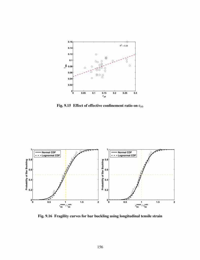
0 0.05 0.1 0.15 0.2 0.25 0.30
0.02
0.04
0.06
0.08
0.1
0.12
0.14
0.16
ρeff
ε bb
R2 = 0.26
Fig. 9.15 Effect of effective confinement ratio on 'bb
0 0.5 1 1.5 20
0.2
0.4
0.6
0.8
1
εbbmeas / ε
bbcalc
Pro
bab
ility
of
Bar
Bu
cklin
g
Normal CDFLognormal CDF
0 0.5 1 1.5 20
0.2
0.4
0.6
0.8
1
∆bbmeas / ∆
bbcalc
Pro
bab
ility
of
Bar
Bu
cklin
g
Normal CDFLognormal CDF
Fig. 9.16 Fragility curves for bar buckling using longitudinal tensile strain
156

0 5 100
0.5
1
1.5
2
L/D
∆b
bm
eas /
∆b
bca
lc
R2 = 0.015
0 0.01 0.02 0.03 0.040
0.5
1
1.5
2
ρl
∆b
bm
eas /
∆b
bca
lc
R2 = 0.00016
0 0.1 0.2 0.3 0.40
0.5
1
1.5
2
P/fcA
g
∆b
bm
eas /
∆b
bca
lc
R2 = 0.2
0 0.1 0.2 0.30
0.5
1
1.5
2
ρeff
∆b
bm
eas /
∆b
bca
lcR2 = 0.00047
0 10 20 30 400
0.5
1
1.5
2
fc
∆b
bm
eas /
∆b
bca
lc
R2 = 0.12
0 1 2 3 4 50
0.5
1
1.5
2
S/db
∆b
bm
eas /
∆b
bca
lc
R2 = 0.009
Fig. 9.17 Effect of key column properties on accuracy of strain estimates of bar buckling
157

9.3.3 Bar Fracture
The mean value of the tensile strain at the onset of bar fracture ('measb f ) was 0.087 with a coefficient
of variation of 28.8%. The mean value and coefficient of variation of the ratios of measured
displacements to calculated displacements associated with the mean value of 'measb f were 1.00 and
27.5%, respectively.
Table 9.7 Bar-fracture estimates based on longitudinal-reinforcement tensile strain
'measb f /'calc
b f "measb f /"calc
b f
Methodology mean cov (%) mean cov (%)
mean 'b f = 0.087 1.00 28.8 1.00 27.5Eq (9.16) 1.00 22.5 1.00 21.2
The tensile strain at the onset of bar fracture is expected to increase with an increase in
effective confinement ratio. This trend is verified in Figure 9.18. In a similar fashion as the bar-
0 0.05 0.1 0.15 0.2 0.250
0.02
0.04
0.06
0.08
0.1
0.12
0.14
0.16
ρeff
ε bf
R2 = 0.4
Fig. 9.18 Effect of effective confinement ratio on 'b f
buckling damage level, an equation was developed to predict the tensile strain at the onset of
longitudinal bar fracture as a function of effective confinement ratio (Equation 9.18). The resulting
equation is nearly identical to the equation developed for bar buckling; therefore the same equation
will be used for both damage states for simplicity.
'calcb f = 0.045+0.30(e f f ≤ 0.15 (9.16)
158

By accounting for the effect of effective confinement ratio with Equation 9.16, the accuracy
of the bar-fracture estimates are improved (Table 9.7). The coefficient of variation for 'measb f /'calc
b f
is reduced from 28.8% using the mean value of 'measb f , to 21.8% using Equation 9.16. Similarly, the
ratio of measured to calculated displacements are reduced from 27.5% to 20.5%. Fragility curves
for this damage state and engineering demand parameter are provided in Figure 9.19.
0 0.5 1 1.5 20
0.2
0.4
0.6
0.8
1
εbfmeas / ε
bfcalc
Pro
bab
ility
of
Bar
Fra
ctu
re
Normal CDFLognormal CDF
0 0.5 1 1.5 20
0.2
0.4
0.6
0.8
1
∆bfmeas / ∆
bfmean
Pro
bab
ility
of
Bar
Fra
ctu
re
Normal CDFLognormal CDF
Fig. 9.19 Fragility curves for bar fracture using longitudinal tensile strain
159

0 5 100
1
2
L/D
∆b
fm
eas /
∆b
fca
lc
R2 = 0.017
0 0.01 0.02 0.03 0.040
1
2
ρl
∆b
fm
eas /
∆b
fca
lc
R2 = 0.061
0 0.1 0.2 0.3 0.40
1
2
P/fcA
g
∆b
fm
eas /
∆b
fca
lc
R2 = 0.37
0 0.1 0.2 0.3 0.40
1
2
ρeff
∆b
fm
eas /
∆b
fca
lc
R2 = 0.002
0 10 20 30 40 500
1
2
fc
∆b
fm
eas /
∆b
fca
lc
R2 = 0.11
0 1 2 3 4 50
1
2
S/db
∆b
fm
eas /
∆b
fca
lc
R2 = 0.017
Fig. 9.20 Effect of key column properties on accuracy of strain estimates of bar fracture
160

9.4 COMPARISON OF DAMAGE ESTIMATES
Damage estimates based on three engineering demand parameters (i.e., drift ratio, plastic rota-
tion, and longitudinal strain) were evaluated in the previous sections. In Table 9.8, this study is
summarized and the accuracy of using the various engineering parameters are compared.
Table 9.8 Comparison of damage estimates
"measdam /"calc
dam
Damage State E.D.P. Equation mean cov (%)
Cover Spalling"calc
sp /L (% ) 1.6 (1−P/Ag f ′c) (1+L/10D) 1.07 34.9
(29 columns) 0calcp sp (%) 1.20 0.98 33.9
'sp 0.008 0.99 34.7
Bar Buckling
"calcbb /L (% ) 3.25
(1+150(e f f db/D
)(1−P/Ag f ′c) (1+L/10D) 1.01 24.7
0calcp bb (%) 0.0009
(1+7.3(e f f
)(1+1.3L/D+3 fydb/D) 1.01 21.6
(33 columns)0calc
p bb (% ) 2.75(1+150(e f f db/D
)(1−P/Ag f ′c) (1+L/10D) 1.01 24.3
'calcbb 0.045+0.25(e f f ≤ 0.15 1.00 23.6
Bar Fracture
"calcb f /L (% ) 3.5
(1+150(e f f db/D
)(1−P/Ag f ′c) (1+L/10D) 0.97 20.0
0calcp b f (%) 0.0009
(1+6.7(e f f
)(1+2.4L/D+1.7 fydb/D) 0.99 16.0
(20 columns)0calc
p b f (% ) 3.0(1+150(e f f db/D
)(1−P/Ag f ′c) (1+L/10D) 0.97 19.6
'calcb f 0.045+0.30(e f f ≤ 0.15 0.96 20.5
As seen in the table, similar levels of accuracy can be obtained by estimating the onset of
damage using drift ratio, plastic rotation, or longitudinal strain. The coefficient of variation for
the ratios of measured to calculated displacements at the onset of spalling was approximately 34%
for all three methods. The coefficient of variations for the onset of bar buckling using the three
methods were 22-25%. For bar fracture, slightly better accuracy can be obtained by using plastic
rotation (coefficient of variation of 16.0%) than drift ratio or longitudinal strain (≈ 21%).
The drift-ratio equations provide a practical correlation between an engineering demand pa-
rameter and key damage states. However, the application of this method is limited to tests in which
the the distance to the point of contraflexure does not vary, the axial load does not vary, and there
is only uniaxial bending. Although estimates based on plastic rotation suffer from the same limi-
tations, plastic rotation is a more versatile engineering demand parameter because it is more easily
calculated in a complex model. The damage estimates based on longitudinal strain overcome the
161

limitations of the drift-ratio and plastic-rotation equations; however they require a more detailed
model in which strains can be monitored.
162

10 Application of Column-Modeling Strategy to More ComplexStructural Models
The column-modeling strategies developed in this report were calibrated and evaluated with ex-
perimental tests of single, equivalent cantilever bridge columns, loaded pseudo-statically in one
dimension. In this chapter, the proposed column-modeling strategies are applied to two more
complex modeling situations. First, the column-modeling strategies are employed to model the
columns of a single bridge bent. The modeling strategies are then used to model shake-table tests
of columns subjected to unidirectional and bidirectional base motions.
10.1 COLUMN BENT TESTS
The proposed distributed-plasticity and lumped-plasticity modeling strategies were used to model
the response of a bridge bent test performed by Makido (2006) at Purdue University (Figure 10.1).
The geometric and material properties of the specimen are provided in tables 10.1 and 10.2, re-
spectively.
10.1.1 Distributed-Plasticity Model
The distributed-plasticity model of the column-bent is illustrated in Figure 10.2. The columns were
modeled with the proposed distributed-plasticity modeling strategy and standard material models
(Chapter 4), with a slip-section at both ends of the column and with 6 integration points, which is
recommended for columns under double curvature (Section 3.1.1). The cross-beam was modeled
as a rectangular force-based beam-column element with six integrations points. However, upon
163

Courtesy of Makido (2006)
Fig. 10.1 Test setup
the completion of the analysis, it was observed that the cross member did not crack, and therefore
could have been modeled as an elastic section with gross section properties.
Accuracy statistics for this modeling strategy are provided in Table 10.3, and the calculated
envelope response is compared to the measured envelope response in Figure 10.3(a). The basic
distributed-plasticity modeling strategy accurately predicts the maximum moment (M.R. = 1.02),
but the model overestimates the initial stiffness (S.R. = 0.69), and does not model the envelope
degradation. The calculated and measured cyclic responses are compared in Figure 10.3(b). As
seen in this figure, this method does not model the strength and stiffness degradation due to cycling
at large deformations.
Ranf (2006) analyzed the same bridge bent in detail. Based on strain measurements in the
bent footing, he recommended bond-strength ratios of #e = 0.6 (compared with #e = 0.9) and #i =
0.3 (compared with #i = 0.45), and a larger bond-compression depth of dcomp = 0.5D (compared
with 1/2 the neutral axis depth at concrete compressive strain of 0.002). Using these values in
the bond-model provides a better estimate of the stiffness ratio (0.94) and therefore a better Epush
164

Table 10.1 Geometric properties of the Purdue bent
Category Property
Column Dimensions
Gross Diameter (mm) 304.8Clear Cover (mm) 26.6Core Diameter (mm) 261.6Column Height (mm) 1524.0Intra-Bent Column Spacing (mm) 1828.8
Column Reinforcement
No. of Longitudinal Bars 16Bar No. 3Longitudinal Steel Ratio (%) 1.56Spiral Bar W2.9Spiral Spacing (mm) 31.8Spiral Bar Diameter (mm) 4.9Spiral Bar Area (mm2) 18.7Transverse Volumetric Steel Ratio (%) 0.90
Beam DimensionsLength (mm) 3149.6Width (mm) 812.8Depth (mm) 457.2Clear Cover (mm) 25.4
Beam ReinforcementNo. of Longitudinal Bars 12Longitudinal Bar No. 5Transverse Bar No. 3Transverse Spacing (mm) 152.4
Table 10.2 Measured material properties for the Purdue bent
Member Property
Columnf ′c (MPa) 29.8fy (MPa) 482.6Es (MPa) 2.00e5
Beamf ′c (MPa) 46.9fy (MPa) 434.32Es (MPa) 2.00e5
value (8.43). The strength estimates did not change, but E f orce and Eenergy improved slightly (Table
10.3).
To capture the strength and stiffness degradation due to cycling at large deformations, a
material model that accounts for this phenomenon is needed. A steel model that accounts for
cyclic degradation is proposed in Chapter 8 (Mohle and Kunnath 2006). However, this model can
not be used reliably in combination with this modeling strategy because the distributed-plasticity
modeling strategy is susceptible to strain concentrations in columns with degrading behavior.
165

Fig. 10.2 Bent model with distributed-plasticity column-modeling strategy
10.1.2 Lumped-Plasticity Model
The modeling strategy for the bridge bent using the proposed lumped-plasticity column-modeling
strategy (Chapter 6) is illustrated in Figure 10.4. A plastic hinge is assumed to form at both ends
of each column, and the length of the plastic hinge was calculated as Lp = 0.05Ls +0.1 fydb/√
f ′c,
where Ls is the distance from column fixity to point of contraflexure (L/2). For these columns, the
calculated plastic-hinge length was 122.3 mm, which is equal to 40% of the column diameter. The
effective stiffness of the elastic portion of the columns was calculated as (EI)e f f = %̂sec(EI)sec,
Table 10.3 Accuracy statistics for column-modeling strategies
Strategy Steel Model Epush(%) S.R. M.R. D.R.(%) E f orce(%) Eenergy(%)
Distr. Standard 11.9 0.7 1.0 8.8 21.0 -63.9Distr., Ranf Bond Standard 8.4 0.9 1.0 8.9 19.3 -50.0Lumped Standard 7.6 0.9 1.1 8.2 19.8 -56.3Lumped Mohle and Kunnath 8.5 0.9 1.0 8.1 13.4 -33.5
166

0 1 2 3 4 5 60
50
100
150
200
250
∆/L (%)
Fo
rce
(KN
)
MeasuredCalculated
(a) Envelope Response
−6 −4 −2 0 2 4 6
−200
−150
−100
−50
0
50
100
150
200
∆/L (%)
Fo
rce
(KN
)
MeasuredCalculated
(b) Cyclic Response
Fig. 10.3 Force-deformation response of bridge bent with distributed-plasticity model andstandard steel
where %̂sec = %(L−3Lp)L−3%Lp
, and %sec = 0.35 + 0.1Ls/D (sections 6.2 and 5.5). For these columns
(EI)e f f ≈ 0.15EcIg. As in the distributed-plasticity model, the cross beam was modeled as a
rectangular, force-based beam-column element with six integrations points. However, upon the
completion of the analysis it was observed that the cross member did not crack, and therefore
could have been modeled as an elastic section with gross section properties.
Accuracy statistics for this modeling strategy are provided in Table 10.3, and the calculated
and measured envelopes are compared in Figure 10.5(a). The proposed modeling strategy accu-
rately models the response of the bridge bent at low levels of deformation; the initial stiffness is
calculated within 15% of the measured response, and the maximum moment is calculated within
5% of the measured response. However, as with the distributed-plasticity method, the lumped-
plasticity method does not model the degrading envelope accurately. The calculated and measured
cyclic responses are compared in Figure 10.5(b). As seen in the figure, this method does not
account for the degradation due to cycling at large deformations.
To overcome this limitation, the more complex steel model (Mohle and Kunnath 2006) de-
scribed in Chapter 8 was used to model the reinforcing steel. The envelope curves and hysteresis
loops for this analysis are presented in Figure 10.6(a) and 10.6(b), and the accuracy statistics are
provided in Table 10.3. As seen in the figures and the table, the Mohle and Kunnath (2006) steel
167

Fig. 10.4 Bent model with lumped-plasticity column-modeling strategy
model significantly improves the estimates of the cyclic response of the bent. The values of E f orce
and Eenergy (13.4% and -33.5%) using the Mohle and Kunnath (2006) steel model are approxi-
mately 60% of the values using the standard steel model (19.8% and -56.3%).
168
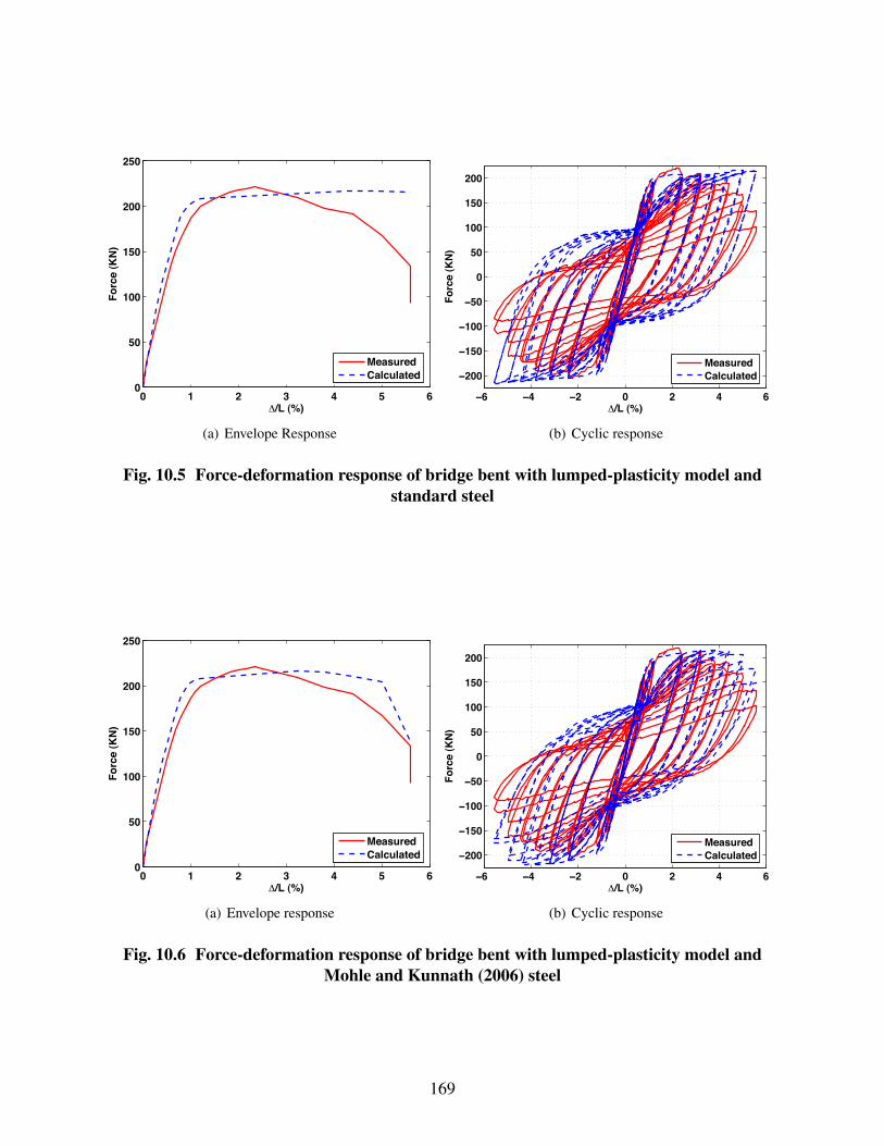
0 1 2 3 4 5 60
50
100
150
200
250
∆/L (%)
Fo
rce
(KN
)
MeasuredCalculated
(a) Envelope Response
−6 −4 −2 0 2 4 6
−200
−150
−100
−50
0
50
100
150
200
∆/L (%)
Fo
rce
(KN
)
MeasuredCalculated
(b) Cyclic response
Fig. 10.5 Force-deformation response of bridge bent with lumped-plasticity model andstandard steel
0 1 2 3 4 5 60
50
100
150
200
250
∆/L (%)
Fo
rce
(KN
)
MeasuredCalculated
(a) Envelope response
−6 −4 −2 0 2 4 6
−200
−150
−100
−50
0
50
100
150
200
∆/L (%)
Fo
rce
(KN
)
MeasuredCalculated
(b) Cyclic response
Fig. 10.6 Force-deformation response of bridge bent with lumped-plasticity model andMohle and Kunnath (2006) steel
169

10.1.3 Flexural Damage
The estimates of cover spalling and bar buckling proposed in Chapter 9 will be applied to the
Purdue bent test in this section. The lumped-plasticity formulation with the standard steel model
was used for this study. The measured drift ratios at the onset of cover spalling and bar buckling
were 1.2%, 3.8% and 4.4% respectively. The calculated engineering demand parameters (drift
ratio, plastic rotation, and longitudinal strain) are reported in Table 10.4. The calculated drift ratios
associated with the calculated engineering demand parameters are also reported along with the
ratios of measured to calculated displacements. As seen in the table, the proposed methodologies
Table 10.4 Damage estimates for purdue bent test
Damage State E.D.P. E.D.P. (%) "calcdam/L(%) "meas
dam /"calcdam
Cover SpallingDrift Ratio 1.1 1.1 1.1Plastic-Rotation 1.5 0.93 1.29Compressive Strain 0.8 1.24 0.96
accurately predict the onset of cover spalling and bar buckling. For this test specimen, longitudinal
strain was the most accurate means of predicting the displacement at the onset of cover spalling
("meassp /"calc
sp = 0.96), whereas drift ratio and plastic-rotation were the most effective means for
predicting bar buckling ("meassp /"calc
sp = 1.05 and 0.95, respectively).
10.2 SHAKE-TABLE TESTS
The proposed column-modeling strategies were used to model shake-table tests performed by
Hachem et al. (2003) at the University of California at Berkeley.
10.2.1 Test Setup and Procedure
The shake-table tests consisted of four identical columns subjected to unidirectional and bidirec-
tional earthquake excitations. The column specimens are illustrated in Figure 10.7, and key geo-
metric and material properties are provided in Table 10.5. Hachem et al. (2003) provides details of
the tests.
Specimens A1 and B1 were subjected to unidirectional excitations, whereas A2 and B2 were
subjected to excitations in two directions (Table 10.6). Two horizontal ground motion time histories
170

Table 10.5 Properties of shake-table specimens
Category Property
ColumnGross Diameter (mm) 406.0Clear Cover (mm) 13.0Column Height (mm) 1630.0
Column Reinforcement
No. of Longitudinal Bars 16Longitudinal Bar Diameter (mm) 12.7Longitudinal Steel Ratio (%) 1.17Spiral Bar Diameter 4.5Spiral Spacing (mm) 31.8Spiral Bar Diameter (mm) 4.9Transverse Volumetric Steel Ratio (%) 0.53
Material Propertiesf ′c (MPa) 39.3fy (MPa) 499.9fys (MPa) 620.5
were used in the tests, and for simplicity, no vertical accelerations were considered. Specimens A1
and A2 were subjected to variations of the Olive View record of the 1994 Northridge earthquake,
whereas columns B1 and B2 were subjected to the 1985 Chile earthquake recorded at the Llolleo
station. Each specimen was initially subjected to runs at or below the yield level to help identify the
elastic response of the specimens. The specimens were then subjected to runs with accelerations
at the design level. Following these runs, the accelerations were amplified to the maximum level,
which matched the capacity of the simulator. The amplitude of the runs at the maximum level were
1.5-2.0 times the amplitude of the design level. The design and maximum level runs were repeated
(in pairs) until failure. The base-acceleration histories of the specimens in the longitudinal and
lateral directions at the design level are presented in Figure 10.8. Table 10.6 lists the peak ground
accelerations (PGA) for the first design level and the first maximum level. The Northridge record
represents a near-fault ground motion with a high-velocity pulse, whereas the Chile record was
chosen to be representative of a long-duration earthquake. The response spectra for the four design
level excitations are presented in Figure 10.9 (damping ratio of 5%).
Table 10.6 Test matrix with pga for 1st design level and 1st maximum level
Peak Ground Accelerations (g)Specimen History design long. design lat. max long. max lat.
A1 Northridge 0.58 - 0.9 -A2 Northridge 0.58 0.65 0.91 0.95B1 Chile 0.48 - 0.87 -B2 Chile 0.47 0.36 0.9 0.67
171
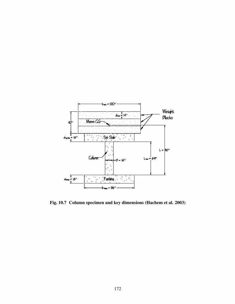
Fig. 10.7 Column specimen and key dimensions (Hachem et al. 2003)
172

0 5 10 15 20 25−0.6
−0.4
−0.2
0
0.2
0.4
time (sec)
Acc
eler
atio
n (g
)Longitudinal Direction of A1 and A2 Specimens
0 5 10 15 20 25−1
−0.5
0
0.5
1
time (sec)
Acc
eler
atio
n (g
)
Lateral Direction of A2 Specimen
0 10 20 30 40 50 60−0.4
−0.2
0
0.2
0.4
0.6
time (sec)
Acc
eler
atio
n (g
)
Longitudinal Direction of B1 and B2 Specimens
0 10 20 30 40 50 60−0.4
−0.2
0
0.2
0.4
0.6
time (sec)
Acc
eler
atio
n (g
)
Lateral Direction of B2 Specimen
Fig. 10.8 Base-acceleration records for test specimens
173

0 0.5 1 1.5 2 2.5 30
0.5
1
1.5
2
2.5A
ccel
erat
ion
(g)
Period (s)
Northridge Long.Northridge Lat.Chile Long.Chile Lat.
Fig. 10.9 Response spectra for base accelerations with a damping ratio of 5%
10.2.2 Modeling Strategies
The distributed-plasticity and lumped-plasticity modeling strategies for the shake-table tests are
illustrated in Figure 10.10. In both modeling strategies, the mass of the block was lumped with its
center of gravity at a distance (LCG) of 812 mm (32 in.) above the top of the column. The mass
of the block (m) was 296 Mg (0.169 kip · s2/in.), and the rotational moment of inertia of the mass
(mR) was 26 Mg · m2 (234 kip · in. · s2). A rigid beam was used to link the top of the column to
the lumped mass. The columns of the specimens were modeled with the strategies proposed in
chapters 4 (distributed-plasticity) and 6 (lumped-plasticity). Rayleigh damping was used in the
model. Based on the damping observed in the shake-table tests, the Raleigh coefficients % and 4
were selected such that the damping ratio was 3.5% at periods of 0.1 and 1.0 seconds (% = 0.4 and
4 = 0.001).
The models described above were evaluated at the first design level and the first maximum
level with the standard cyclic material models, and the modified material models proposed in Chap-
ter 8. To account for the effects of preliminary ground motions, all runs prior to the first design
174

(a) Distributed-plasticity (b) Lumped-plasticity
Fig. 10.10 Modeling strategies for shake-table tests
level and maximum level were considered in the analysis. Table 10.7 describes the six model-
ing variations evaluated in this study. The distributed-plasticity model was evaluated with perfect
crack closure (r = 0.0) and imperfect crack closure (r = 1.0) and the standard steel model. The
lumped-plasticity method was evaluated with both variations of crack closure assumptions, and
the two proposed steel models: Menegotto-Pinto and Mohle and Kunnath (2006) (Cf = 0.26 and
Cd = 0.45).
10.2.3 Response Maxima and Hysteretic Energy
Maximum tip displacement, maximum base moment, maximum base shear, and hysteretic energy
were used to evaluate the six modeling strategies. The hysteretic energy is the area within the
hysteretic force-deformation curves and is calculated with Equation 7.3.
The accuracy of each model is shown graphically in Figure 10.11 (design level-lateral),
Figure 10.12 (design level-longitudinal), Figure 10.13 (maximum level-lateral), and Figure 10.14
175

Table 10.7 Modeling variations for shake-table specimens
Modeling Strategy Steel Model Crack Closure Name
Distributed Standard r = 0.0 cmax = 0.0 DP-S-PCStandard r = 1.0 cmax = 0.01 DP-S-IC
Lumped
Standard r = 0.0 cmax = 0.0 LP-S-PCStandard r = 1.0 cmax = 0.01 LP-S-ICMohle r = 0.0 cmax = 0.0 LP-M-PCMohle r = 1.0 cmax = 0.01 LP-M-IC
(maximum level-longitudinal). As seen in the figures, all column-modeling variations predict the
maximum displacement, shear force, and hysteretic energy within 30% of the measured response
for both earthquake records at both levels of excitation in the longitudinal and lateral directions.
However, the modeling variations were less accurate when predicting the maximum base moments,
especially the lumped-plasticity methods in the lateral direction. Also seen in the figures, the crack
closure variations do not significantly affect any of the response maxima, which leaves two strate-
gies to compare: distributed plasticity to lumped plasticity (both with standard steel), and the
lumped-plasticity variation with standard steel to the lumped-plasticity variation with degrading
steel.
No significant trends can be observed in the maximum displacements, and hysteretic en-
ergy estimates calculated with the distributed-plasticity and lumped-plasticity estimates (both with
standard steel) at either earthquake record or excitation level. However, the ratios of measured to
calculated base moments are larger for the distributed-plasticity methodology for both earthquake
records at both levels of excitation in the longitudinal direction. However the opposite trend is
observed in the lateral direction. Similarly, the ratios of measured to calculated shear forces are
larger (on average) for the distributed-plasticity methodology for both earthquake records and both
excitation levels in both directions.
On average, the ratios of measured to calculated base moments and shear forces are greater
for the lumped-plasticity methodology with standard steel than with the degrading steel model. No
other significant trends are observed when comparing these two variations.
176

.
Displacement Base Moment Shear Force Energy0
0.5
1
1.5
Mea
sure
d / C
alcu
late
d
A2 Design Level − Lateral Direction
DP−S−PCDP−S−IC)LP−S−PCLP−S−ICLP−M−PCLP−M−IC
Displacement Base Moment Shear Force Energy0
0.5
1
1.5
Mea
sure
d / C
alcu
late
d
B2 Design Level − Lateral Direction
DP−S−PCDP−S−IC)LP−S−PCLP−S−ICLP−M−PCLP−M−IC
Fig. 10.11 Ratio of measured to calculated results for various response maxima in thelateral direction at first design level
177

Displacement Base Moment Shear Force Energy0
0.5
1
1.5
Mea
sure
d / C
alcu
late
d
A1 Design Level − Longitudinal Direction
DP−S−PCDP−S−IC)LP−S−PCLP−S−ICLP−M−PCLP−M−IC
Displacement Base Moment Shear Force Energy0
0.5
1
1.5
Mea
sure
d / C
alcu
late
d
A2 Design Level − Longitudinal Direction
DP−S−PCDP−S−IC)LP−S−PCLP−S−ICLP−M−PCLP−M−IC
Displacement Base Moment Shear Force Energy0
0.5
1
1.5
Mea
sure
d / C
alcu
late
d
B1 Design Level − Longitudinal Direction
DP−S−PCDP−S−IC)LP−S−PCLP−S−ICLP−M−PCLP−M−IC
Displacement Base Moment Shear Force Energy0
0.5
1
1.5
Mea
sure
d / C
alcu
late
d
B2 Design Level − Longitudinal Direction
DP−S−PCDP−S−IC)LP−S−PCLP−S−ICLP−M−PCLP−M−IC
Fig. 10.12 Ratio of measured to calculated results for various response maxima in thelongitudinal direction at first design level
178

Displacement Base Moment Shear Force Energy0
0.5
1
1.5
Mea
sure
d / C
alcu
late
d
A2 Maximum Level − Lateral Direction
DP−S−PCDP−S−IC)LP−S−PCLP−S−ICLP−M−PCLP−M−IC
Displacement Base Moment Shear Force Energy0
0.5
1
1.5
Mea
sure
d / C
alcu
late
d
B2 Maximum Level − Lateral Direction
DP−S−PCDP−S−IC)LP−S−PCLP−S−ICLP−M−PCLP−M−IC
Fig. 10.13 Ratio of measured to calculated results for various response maxima in thelateral direction at first maximum level
179

Displacement Base Moment Shear Force Energy0
0.5
1
1.5
Mea
sure
d / C
alcu
late
d
A1 Maximum Level − Longitudinal Direction
DP−S−PCDP−S−IC)LP−S−PCLP−S−ICLP−M−PCLP−M−IC
Displacement Base Moment Shear Force Energy0
0.5
1
1.5
Mea
sure
d / C
alcu
late
d
A2 Maximum Level − Longitudinal Direction
DP−S−PCDP−S−IC)LP−S−PCLP−S−ICLP−M−PCLP−M−IC
Displacement Base Moment Shear Force Energy0
0.5
1
1.5
Mea
sure
d / C
alcu
late
d
B1 Maximum Level − Longitudinal Direction
DP−S−PCDP−S−IC)LP−S−PCLP−S−ICLP−M−PCLP−M−IC
Displacement Base Moment Shear Force Energy0
0.5
1
1.5
Mea
sure
d / C
alcu
late
d
B2 Maximum Level − Longitudinal Direction
DP−S−PCDP−S−IC)LP−S−PCLP−S−ICLP−M−PCLP−M−IC
Fig. 10.14 Ratio of measured to calculated results for various response maxima in thelongitudinal direction at first maximum level
180

10.2.4 Residual Displacements
To evaluate the accuracy of the residual displacements calculated with the six modeling variations,
the calculated residual displacements ("rc/L) in the longitudinal direction are plotted versus the
measured residual displacements ("rm/L) for both earthquake records at both levels of excitation
(design and maximum) in Figure 10.15.
−1 −0.5 0 0.5 1 1.5 2 2.5 3−1
−0.5
0
0.5
1
1.5
2
2.5
3
∆rm
/L (%)
∆rc
/L (
%)
DP−S−PCDP−S−IC)LP−S−PCLP−S−ICLP−M−PCLP−M−IC
−1 −0.5 0 0.5 1 1.5 2 2.5 3−1
−0.5
0
0.5
1
1.5
2
2.5
3
∆rm
/L (%)
∆rc
/L (
%)
DP−S−PCDP−S−IC)LP−S−PCLP−S−ICLP−M−PCLP−M−IC
Fig. 10.15 Comparison of measured and calculated residual displacements
The following can be observed in the figure.
1. The model variations are more accurate at predicting the residual displacements at the design
level than at the maximum level.
2. The distributed-plasticity variations overestimate (on average) the residual displacements for
both earthquake records and both levels of excitation.
3. The imperfect crack closure variation improves the estimates of residual displacements for
the distributed-plasticity model.
4. The imperfect crack closure assumption does not improve the residual displacements calcu-
lated with the lumped-plasticity variations with standard steel or degrading steel.
The normalized residual displacement error (Erd) is used to further evaluate the effective-
ness of the modeling strategies’ abilities to predict residual displacements. This error measure is
defined as the difference between measured ("measres ) and calculated ("calc
res ) residual displacements
181

normalized by the maximum measured displacement, as follows.
Erd = abs(
"measres −"calc
res"meas
max
)(10.1)
Erd is plotted for each modeling strategy and each column for the first design level and
first maximum level in Figure 10.16. As noted previously, the imperfect crack closure assumption
improves the estimate of residual displacements for the distributed-plasticity strategy. However, the
same can not be said for the lumped-plasticity methodology; there is no significant trend for this
methodology. The effect of the crack closure variations may be more evident in the distributed-
plasticity methodology because the stress-deformation response of the concrete in the bond-slip
section was modeled with the the crack closure variations, and a significant portion of the total
deformation is attributed to this section. Therefore, the model is more sensitive to this parameter.
No other significant trends can be observed in the data.
More work is needed to improve estimates of residual displacements. One possible improve-
ment would be to remove the limitation on the imperfect crack closure concrete model that does
not allow compression stress in the concrete while it still has tensile strain. This would amplify the
effect of imperfect crack closure, and may improve estimates of residual displacements.
182

A1 A2 B1 B20
0.05
0.1
0.15
0.2
0.25N
orm
aliz
ed R
esid
ual D
isp.
Err
orDesign Level−LongitudinalDirection
DP−S−PCDP−S−IC)LP−S−PCLP−S−ICLP−M−PCLP−M−IC
A1 A2 B1 B20
0.05
0.1
0.15
0.2
0.25
Nor
mal
ized
Res
idua
l Dis
p. E
rror
Maximum Level−LongitudinalDirection
DP−S−PCDP−S−IC)LP−S−PCLP−S−ICLP−M−PCLP−M−IC
A1 A2 B1 B20
0.05
0.1
0.15
0.2
0.25
Nor
mal
ized
Res
idua
l Dis
p. E
rror
Design Level−LateralDirection
DP−S−PCDP−S−IC)LP−S−PCLP−S−ICLP−M−PCLP−M−IC
A1 A2 B1 B20
0.05
0.1
0.15
0.2
0.25
Nor
mal
ized
Res
idua
l Dis
p. E
rror
Maximum Level−LateralDirection
DP−S−PCDP−S−IC)LP−S−PCLP−S−ICLP−M−PCLP−M−IC
Fig. 10.16 Normalized residual displacement errors at first design level and first maximumlevel in longitudinal and lateral directions
183

10.2.5 Flexural Damage
In Chapter 9, equations were developed to predict the drift ratio ("dam/L), plastic rotation (0p dam),
and longitudinal strain ('dam) at the onset of cover spalling and bar buckling. In this section, these
damage equations are applied to the shake-table tests to evaluate their accuracy. The following
analysis was carried out with only one model variation from the previous section: the lumped-
plasticity variation with standard steel and perfect crack closure.
Application of the drift-ratio equations to this structural model is difficult because the dis-
tance from the base of the column to the point of contraflexure varies throughout the duration of the
earthquake. This phenomenon complicates the calculation of the demand drift ratio, as well as the
calculated drift ratios at the onset of cover spalling and bar buckling (from the damage equations).
The varying inflexion point also complicates the calculation of the plastic rotation at the onset
of bar buckling. Some simplifications must be made to apply the drift-ratio and plastic-rotation
methodologies to this structural system. For a preliminary analysis, the system is assumed to act
as a cantilever system, where the distance to the point of contraflexure is constant and is equal to
the height of the column. This assumption is not accurate, but is performed here to demonstrate
the process of applying the methodologies. The damage estimates based on strain overcome this
limitation, and should provide a more effective means of estimating damage in more complicated
systems.
The results of the preliminary study are summarized in tables 10.8 (cover spalling) and 10.9
(bar buckling). In these tables the calculated engineering demand parameters (from the damage
equations) at the onset of the damage states are reported, along with the maximum calculated
engineering demand parameters before (“pre”) and immediately after (“post”) the run where the
damage state was observed. The probability (based on statistics from Chapter 9) that cover spalling
or bar buckling will have occurred before and after the observed damage run are also provided.
As seen in Table 10.8, the onset of cover spalling is accurately predicted with the proposed
drift-ratio and plastic-rotation methodologies (with current inflexion point assumption). Whereas,
the strain estimates accurately predict cover spalling in specimens A1 and A2, but only estimate a
10% probability of spalling in B1 and 30% probability in B2.
The bar buckling estimates were not as clean. Although some methods calculate a 50%
probability of bar buckling after the reported damage run, the same probability is calculated for the
184

runs prior to the observed damage run. These results suggest that estimates of bar buckling may be
improved if cycling is considered.
Table 10.8 Summary of spalling estimates
"sp/L (%) 0p sp (%) 'sp (%)
pre post pre post pre post
col. calc max pr. max pr. calc max pr. max pr. calc max pr. max pr.
A1 2.1 0.9 4% 4.9 100% 1.5 0.0 0% 3.8 100% 0.8 0.1 1% 1.5 100%A2 2.1 0.9 5% 4.9 100% 1.5 0.0 0% 3.8 100% 0.8 0.1 1% 1.4 99%B1 2.1 1.1 7% 3.0 81% 1.5 0.1 0% 1.9 78% 0.8 0.1 1% 0.4 10%B2 2.1 1.3 12% 3.0 83% 1.5 0.3 1% 2.0 85% 0.8 0.2 1% 0.6 30%
Table 10.9 Summary of bar-buckling estimates
"bb/L (%) 0p bb (%) 'bb (%)
pre post pre post pre post
col. calc max pr. max pr. calc max pr. max pr. calc max pr. max pr.
A1 6.0 6.2 54% 6.2 54% 5.9 5.2 27% 5.2 27% 6.7 4.5 8% 5.9 32%A2 6.0 5.5 36% 5.5 36% 5.9 4.5 13% 4.5 13% 6.7 6.7 50% 6.7 50%B1 6.0 3.0 2% 4.5 15% 5.9 1.9 0% 3.4 3% 6.7 3.4 2% 5.9 30%B2 6.0 4.5 14% 4.5 14% 5.9 3.4 2% 3.4 2% 6.7 5.0 15% 5.0 15%
185

11 Summary and Conclusions
It is important to characterize the performance of bridges during earthquakes because they are in-
tegral components of transportation networks. Loss of bridge function can have severe economic
consequences, and and consequences to life safety when bridges are critical links in lifelines to
emergency facilities, which are particularly important after a disasters. Although damage to other
bridge elements can have economic and life-safety impacts, reinforced concrete columns are often
the most vulnerable elements in a bridge, and column failure can have catastrophic consequences.
Excessive deformations can result in spalling of cover concrete, buckling of longitudinal reinforce-
ment, bar fracture, reduction of flexural capacity, and eventually, structural collapse.
The objective of this project was to develop, calibrate, and evaluate column-modeling strate-
gies to accurately model column behavior under seismic loading, including global forces and lo-
cal deformations, as well as progression of damage. The models were calibrated using the ob-
served cyclic force-deformation responses and damage progression observations of 37 tests of
spiral-reinforced columns, representative of modern bridge construction (Section 1.3). This effort
is an important step toward implementing performance-based earthquake engineering for modern
reinforced concrete bridges.
11.1 CROSS-SECTION MODELING
The accuracy of the column-modeling strategies presented in this report depend on the accuracy
of the cross-section model, and in turn the accuracy of the material constitutive models and the
cross-section discretization strategy. Uniform and nonuniform radial discretization strategies were
presented in Chapter 2. Based on convergence considerations, the following conclusions were
187

drawn.
1. A uniform radial discretization scheme with 10 radial core divisions, 20 transverse core
divisions, 1 radial cover division, and 20 transverse cover divisions provides a sufficient
mesh (220 total fibers) for modeling the section response of a reinforced concrete column.
2. A nonuniform discretization scheme with a coarser mesh near the center of the column can
be used with an insignificant loss of accuracy. The recommended nonuniform discretization
strategy has 140 total fibers. The coarse mesh at the center of the column has a radius of
half the column depth with 10 transverse divisions and 2 radial divisions. The denser core
concrete mesh has 20 transverse divisions and 5 radial divisions, while the cover concrete
has 20 transverse divisions and 1 radial division.
11.2 ENVELOPE RESPONSE OF DISTRIBUTED-PLASTICITY COLUMN-MODELINGSTRATEGY
A distributed-plasticity modeling strategy was described, calibrated, and evaluated based on the
envelope response of the element in chapters 3 and 4. In the proposed distributed-plasticity mod-
eling strategy, a nonlinear force-based fiber beam-column element, a zero-length bond section,
and an aggregated elastic-shear section were combined to model the flexural, bond slip and shear
components of the total tip deflection of a column. In this formulation, nonlinear deformations are
allowed to form anywhere along the height of the column. The following conclusions are made
about the envelope response of the proposed distributed-plasticity modeling strategy.
1. The proposed distributed-plasticity column-modeling strategy provided an accurate means
of estimating envelope response of the bridge columns. Key accuracy statistics are presented
in Table 11.1.
2. The optimal model parameters were as follows.
· Strain-Hardening Ratio, b = 0.01.· Elastic and Inelastic Bond-Strength Ratios, #e = 0.9 and #i = 0.45.· Development Bar Stress, )d = 0.25)y.· Number of Integration Points, Np = 5 (Cantilever Columns), Np = 6 (Double Curva-
ture).· Bond-Model Effective Compression Depth, dcomp =1/2 neutral axis depth at 'c = 0.002.
188

· Shear-Stiffness Ratio, $ = 0.4.
3. The calculated response of the distributed-plasticity modeling strategy is not sensitive to the
integration scheme for columns with hardening section behavior. However, the calculated
local deformations varied with the integration scheme for columns with perfectly-plastic
section responses. For columns with degrading section responses, both the local deforma-
tions and global forces vary with the integration scheme. This subjectivity is due to strain
localizations that occur at the integration point with the maximum moment.
Table 11.1 Accuracy statistics for envelope response of column-modeling strategies
Distributed-Plasticity Lumped-PlasticityStatistic Epush(%) S.R. M.R. D.R. Epush(%) S.R. M.R. D.R.
Mean 7.4 0.84 1.03 -0.51 7.9 1.00 1.05 -1.11c.o.v. (%) - 15.6 7.9 - - 16.1 8.4 -
11.3 ENVELOPE RESPONSE OF LUMPED-PLASTICITYCOLUMN-MODELING STRATEGY
The envelope response of a lumped-plasticity column-modeling strategy was presented, calibrated,
and evaluated in chapters 5 and 6. In this approach, the nonlinear deformations of the lumped-
plasticity formulation are assumed to be concentrated in the prescribed plastic-hinge region of the
column. In the lumped-plasticity formulation, there are not separate model components to account
for the shear and bond slip components of the total tip deflection. The effects of these deformation
components are accounted for in the plastic-hinge length. The following conclusions were drawn
about the envelope response of the proposed lumped-plasticity formulation.
1. The envelope response of modern reinforced concrete bridge columns can modeled accu-
rately with the proposed lumped-plasticity modeling strategy. Key accuracy statistics are
provided in Table 11.1.
2. The effective cross-section stiffness, (EI)e f f , of the elastic portion of the lumped-plasticity
column model can be estimated as a function of the gross cross-section stiffness, EcIg, or
secant stiffness, (EI)sec = My/!y, with the following equations.
(EI)e f f = %calcg EcIg (11.1)
189

(EI)e f f = %calcsec (EI)sec (11.2)
where Ec is the modulus of elasticity of the concrete, Ig is the moment of inertia of the gross
cross section. The parameters %g and %sec are stiffness modification ratios that account for
the effects of bar slip, shear deformation, and axial load. These parameters can be calculated
with the following equations.
%calcg = 0.15+0.03
LD
+0.95P
Ag f ′c+0.08(l ≤ 1.0 (11.3)
%calcsec = 0.35+0.1
LD≤ 1.0 (11.4)
where L is the distance from the point of maximum moment to the point of contraflexure,
D is the depth of the column, fy and db are the yield stress and diameter of the longitudinal
reinforcement, P is the axial load, Ag is the gross area of the cross section, f ′c is the concrete
compressive strength, and (l is the longitudinal-reinforcement ratio.
3. The length of the plastic-hinge region of the lumped-plasticity column-modeling strategy
can be calculated with the following equation.
Lp = 0.05L+0.1fydb√
f ′c≤ L
4(11.5)
11.4 CYCLIC RESPONSE OF MODELING STRATEGIES WITH STANDARDMATERIAL MODELS
The initial calibration and evaluation of the proposed distributed-plasticity (Chapter 4) and lumped-
plasticity (Chapter 6) modeling strategies were based on the envelope response of the columns. In
Chapter 7, the cyclic response of the modeling strategies (with standard material models) was
evaluated, and inaccuracies were identified. Based on this study, the following conclusions were
made.
1. Similar accuracy can be obtained using either of the distributed-plasticity or lumped-plasticity
column-modeling strategies with standard cyclic material models (Giuffre-Menegotto-Pinto
steel and Karsan-Jirsa concrete). Key accuracy statistics are presented in Table 11.2. The
mean values of the force errors (E f orce) were 16.1% and 15.7% for both the distributed-
plasticity and lumped-plasticity models, respectively. The mean values of the energy errors
190

(Eenergy) were -23.7% and -19.9% for the distributed-plasticity and lumped-plasticity mod-
els, respectively.
2. The proposed modeling strategies with standard cyclic material models accurately predict the
cyclic response of the columns at low levels of ductility and cycling. However, the models
failed to capture the effects of degradation due to cycling at high levels of ductility.
Table 11.2 Accuracy statistics for cyclic response of column-modeling strategies
E f orce (%) Eenergy (%)Modeling Strategy (Steel Model) mean min max mean min max
Distributed-Plasticity (Standard) 16.1 6.6 44.7 -23.7 -109.7 13.4Lumped-Plasticity (Standard) 15.7 6.5 45.1 -19.9 -112.7 20.7Lumped-Plasticity (Mohle and Kunnath) 12.6 5.9 23.9 -4.5 -47.2 31.6
11.5 IMPROVED CYCLIC MATERIAL MODELS
The cyclic modeling inaccuracies identified in Chapter 7 were addressed in Chapter 8. A steel
material model proposed by Mohle and Kunnath (2006), which accounts for degradation due to
cycling, was presented, calibrated, and evaluated. A concrete model that accounts for imperfect
crack closure was also developed and evaluated in this chapter. The following conclusions were
made based on the results of this study.
1. The use of a more complex steel constitutive model (Mohle and Kunnath 2006), which in-
cludes degradation due to cycling, improved the accuracy of the lumped-plasticity column-
modeling strategy (Table 11.2). The mean force error (E f orce) decreased from 15.7% with
the standard steel model to 12.6% with the Mohle and Kunnath (2006) steel model and cal-
ibrated parameters (Cf = 0.26 and Cd = 0.45). The mean energy error (Eenergy) improved
from -19.9% to -4.5%.
2. The distributed-plasticity modeling strategy is susceptible to strain concentrations in perfectly-
plastic or degrading members (Section 11.2). Therefore, the Mohle and Kunnath (2006) steel
constitutive model should be used to model degradation due to cycling only in the lumped-
plasticity column-modeling strategy.
3. The modification to the standard Karsan and Jirsa cyclic material behavior to account for
imperfect crack closure did not significantly affect the accuracy of the proposed modeling
191

strategies.
11.6 COLUMN FLEXURAL DAMAGE
In Chapter 9, a series of damage models were developed that link three engineering demand param-
eters (drift ratio, plastic rotation, longitudinal strain) with three damage states (cover spalling, bar
buckling, and bar fracture). Table 11.3 summarizes this study and provides key accuracy statistics.
Table 11.3 Comparison of damage estimates
"measdam /"calc
dam
Damage State E.D.P. Equation mean cov (%)
Cover Spalling"calc
sp /L (% ) 1.6 (1−P/Ag f ′c) (1+L/10D) 1.07 34.9
(29 columns) 0calcp sp (%) 1.20 0.98 33.9
'sp 0.008 0.99 34.7
Bar Buckling
"calcbb /L (% ) 3.25
(1+150(e f f db/D
)(1−P/Ag f ′c) (1+L/10D) 1.01 24.7
0calcp bb (% ) 2.75
(1+150(e f f db/D
)(1−P/Ag f ′c) (1+L/10D) 1.01 24.3
(33 columns)'calc
bb 0.045+0.25(e f f ≤ 0.15 1.00 23.6
Bar Fracture
"calcb f /L (% ) 3.5
(1+150(e f f db/D
)(1−P/Ag f ′c) (1+L/10D) 0.97 20.0
0calcp b f (% ) 3.0
(1+150(e f f db/D
)(1−P/Ag f ′c) (1+L/10D) 0.97 19.6
(20 columns)'calc
b f 0.045+0.30(e f f ≤ 0.15 0.96 20.5
1. Similar levels of accuracy can be obtained by estimating the onset of damage using drift
ratio, plastic rotation, or longitudinal strain (Table 11.3). The coefficients of variation for the
ratios of measured to calculated displacements at the onset of spalling were approximately
35% for all three methods. The coefficients of variation for the onset of bar buckling using
the three methods were approximately 24%. For bar fracture, the coefficient of variations
were approximately 21% for all three methods.
2. The drift-ratio equations provide a practical correlation between an engineering demand pa-
rameter and key damage states. However, the application of this method is limited to tests
in which the the distance to the point of contraflexure does not vary, the axial load does not
vary, and there is only uniaxial bending. Although estimates based on plastic rotation suffer
192

from the same limitations, plastic rotation is a more versatile engineering demand parame-
ter because it is more easily calculated in a complex model. The damage estimates based
on longitudinal strain overcome the limitations of the drift-ratio and plastic-rotation equa-
tions, however they require a more detailed model in which strains can be monitored, and
the calculated strains depend on the assumed plastic-hinge length.
11.7 APPLICATION OF COLUMN-MODELING STRATEGIES TO MORE COMPLEXSTRUCTURES
The proposed modeling strategies were evaluated for use in more complex structures in Chapter 10.
The models were first used to model the columns of a two-column bent test performed at Purdue
University (Makido 2006). The modeling strategies were then used to model the dynamic response
of shake-table specimens tested at the University of California at Berkeley (Hachem, Mahin, and
Moehle 2003). The following conclusions were drawn from this study.
1. The proposed modeling strategies provided an accurate means of predicting the force-
deformation response and damage progression of the column bent tests (Table 11.4). The
stiffness estimates improved by using the bond properties identified by Ranf (2006). The
Mohle and Kunnath (2006) steel constitutive model provided a more accurate estimate of
cyclic response.
Table 11.4 Accuracy statistics for bent specimen
Strategy Steel Model Epush(%) S.R. M.R. D.R.(%) E f orce(%) Eenergy(%)
Distr. Standard 11.9 0.7 1.0 8.8 21.0 -63.9Distr., Ranf Bond Standard 8.4 0.9 1.0 8.9 19.3 -50.0Lumped Standard 7.6 0.9 1.1 8.2 19.8 -56.3Lumped Mohle and Kunnath 8.5 0.9 1.0 8.1 13.4 -33.5
2. The proposed column-modeling strategies provided an accurate means of estimating re-
sponse maxima, hysteretic energy dissipation, and cover spalling in the shake-table spec-
imens tested at the University of California at Berkeley. However, the models were not
successful at predicting residual displacements nor the effect of cumulative deformation on
bar buckling.
193

3. Similar accuracy can be obtained by using either the distributed-plasticity or lumped-plasticity
column-modeling strategies. It is necessary to use the distributed-plasticity modeling strat-
egy when the location of the yielding is unknown (e.g., modeling a column partially em-
bedded in the soil). In situations in which the location of the plastic hinge is known (e.g.,
cantilever column), the lumped-plasticity method is preferred. This method is more efficient
(only one nonlinear integration point) and the localization issues are governed by a calcu-
lated plastic hinge (which has a physical interpretation), rather than a selected integration
scheme.
11.8 RECOMMENDATIONS FOR FURTHER WORK
The following suggestions are made for further work.
1. The effect of cycling on cover spalling, bar buckling, and bar fracture should be evaluated
further.
2. The return drift and return strain models proposed by Freytag (2006) to estimate bar buckling
should be used to evaluate the column tests in the bridge column dataset used in this report.
3. The effect of varying the damping ratio on the calculated response of the shake-table speci-
mens should be evaluated.
4. The imperfect crack closure model proposed in Chapter 10 should be improved to allow
compressive stress while the concrete is still in the tensile strain region.
194

REFERENCES
ACI 318 (2002). Building Code Requirements for Structural Concrete. American Concrete In-stitute.
Berry, M. and M. Eberhard (2003). Performance Models for Flexural Damage in ReinforcedConcrete Columns,. PEER 2003/18, Pacific Earthquake Engineering Research Center,Berkeley, CA.
Berry, M. and M. Eberhard (2005, July). Practical performance model for bar buckling. Journalof the Structural Engineering ASCE 131(7), 1060–70.
Berry, M., M. Parish, and M. O. Eberhard (2004). PEER Structural Performance Database.Pacific Earthquake Engineering Research Center, Berkeley, CA.
Chang, G. and J. Mander (1994). NCEER Technical Report 94-0006.
Cheok, G. S. and W. C. Stone (1986). Behavior of 1/6-scale model bridge columns subjected tocycle inelastic loading, NBSIR 86-3494. U.S. National Institute of Standards and Technol-ogy, Gaithersburg, Md.
Coleman, J. and E. Spacone (2001, November). Localization issues in force-based frame ele-ments. Journal of the Structural Engineering ASCE 127(11), 1257–1265.
Corley, G. W. (1966). Rotational capacity of reinforced concrete beams. Journal of the Struc-tural Division ASCE 92(ST5), 121–146.
Dhakal, R. and K. Maekawa (2002). Modeling for postyield buckled of reinforcement. Journalof the Structural Engineering ASCE 128(9), 1139–1147.
Freytag, D. (2006). Bar buckling in reinforced concrete bridge columns. Master’s thesis, Uni-versity of Washington.
Ghee, A. B., M. J. N. Priestley, and R. Park (1981). Ductility of reinforced concrete bridgepiers under seismic loading, Report 81-3. Department of Civil Engineering, University ofCanterbury, Christchurch, New Zealand.
Gomes, A. and J. Appleton (1997). Nonlinear cyclic stress-strain relationship of reinforcing barsincluding buckling. Journal of the Structural Engineering ASCE 19(10).
Hachem, M. M., S. A. Mahin, and J. P. Moehle (2003). Performance of Circular ReinforcedConcrete Bridge Columns under Bidirectional Earthquake Loading. PEER 2003/06, PacificEarthquake Engineering Research Center, Berkeley, CA.
Henry, L. and S. A. Mahin (1999). Study of buckling of longitudinal bars in reinforced concretebridge columns. Report to the California Dept. of Transportation.
Hose, Y. D., F. Seible, and M. J. N. Priestley (1997). Strategic relocation of plastic hinges inbridge columns, Structural Systems Research Project, 97/05. University of California, SanDiego.
Johnson, N., R. T. Ranf, M. Saiidi, D. Sanders, and M. Eberhard (2006, August). Shake tablestudies of a large scale two-span reinforced concrete bridge frame. Proceedings from theEighth National Conference on Earthquake Engineering.
195

Kowalsky, M., M. Priestley, and F. Seible (1999). Shear and flexural behavior of lightweightconcrete bridge columns in seismic regions. ACI Structural Journal.
Kunnath, S., A. El-Bahy, A. Taylor, and W. Stone (1997). Cumulative seismic damage of rein-forced concrete bridge piers, NCEER-97-0006. National Center for Earthquake EngineeringResearch, Buffalo, N.Y.
Lehman, D. E. and J. P. Moehle (2000). Seismic Performance of Well-Confined Concrete BridgeColumns. PEER 1998/01, Pacific Earthquake Engineering Research Center, Berkeley, CA.
Makido, A. (2006). Pseudo-static tests of bridge components. Master’s thesis, Purdue Univer-sity.
Mander, J., M. Priestley, and R. Park (1988, August). Theoretical stress-strain model for con-fined concrete. Journal of the Structural Division ASCE 114(8), 1804–1826.
MATLAB (2005). Version 7.01. The Mathworks, www.mathworks.com.
Mattock, A. (1967). Rotational capacity of reinforced concrete beams. Journal of StructuralDivision, ASCE 93(ST2).
Mazzoni, S., F. McKenna, G. L. Fenves, and et al (2006). Open system for earthquake engineer-ing simulation user manual. www.opensees.berkeley.edu.
Mohle, J. and S. Kunnath (2006). Reinforcing steel. OpenSEES User’s Manual,www.opensees.berkeley.edu.
Moyer, M. and M. Kowalsky (2001). Influence of tension strain on buckling of reinforcement inrc bridge columns. Master’s thesis, North Carolina State University.
Munro, I., R. Park, and M. Priestley (1976). Seismic Behaviour of Reinforced ConcreteBridge Piers, Report 76-9. Department of Civil Engineering, University of Canterbury,Christchurch, New Zealand.
OpenSees Development Team (2002). Opensees: Open system for earthquake engineering sim-ulations. Version 1.5, Berkeley, CA.
Parish, M. (2001). Accuracy of seismic performance methodologies for rectangular reinforcedconcrete columns. Master’s thesis, University of Washington.
Park, R. and T. Paulay (1975). Reinforced Concrete Structures. New York: John Wiley andSons, Inc.
Pontangaroa, R., M. Priestley, and R. Park (1979). Ductility of Spirally Reinforced ConcreteColumns Under Seismic Loading, Report 79-8. Department of Civil Engineering, Universityof Canterbury, Christchurch, New Zealand.
Priestley, M., F. Seible, and G. Calvi (1996). Seismic Design and Retrofit of Bridges. New York:John Wiley and Sons, Inc.
Ranf, R. (2006). Performance Based Evaluation of Seismic Modeling Strategies for Bridges. Ph.D. thesis, Univeristy of Washington, Seattle.
Sachem, M. (2003). Performance of Circular Reinforced Concrete Bridge Columns Under Bidi-rectional Earthquake Loading. PEER 2003/06, Pacific Earthquake Engineering ResearchCenter, Berkeley, CA.
Scott, M. and G. Fenves (2006, February). Plastic hinge integration methods for force-basedbeam-column elements. Journal of the Structural Engineering ASCE 132(2), 244–252.
196

Stanton, J. (1979). The Development of a Mathematical Model to Predict the Flexural Responseof Reinforced Concrete Beams to Cyclic Loads, Using System Identification. Ph. D. thesis,University of California at Berkeley, Berkeley, California.
Stone, W. C. and G. S. Cheok (1989). Inelastic behavior of full-scale bridge columns subjectedto cyclic loading, NIST Building Science Series 166. U.S. National Institute of Standardsand Technology, Gaithersburg, Md.
Taucer, F., E. Spacone, and F. Filippou (1991). A Fiber Beam-Column Element for SeismicResponse Analysis of Reinforced Concrete Structures. UCB/EERC-91/17, Earthquake Engi-neering Research Center, Berkeley, CA.
Vu, N. D., M. J. N. Priestley, F. Seible, and G. Benzoni (1998). Seismic response of well con-fined circular reinforced concrete columns with low aspect ratios, 97/05. Proc., 5th CaltransSeismic Research Workshop, Sacramento, California.
Wong, Y. L., T. Paulay, and M. J. N. Priestley (1990). Squat circular bridge piers under multi-directional seismic attack, Report 90-4. Department of Civil Engineering, University of Can-terbury, Christchurch, New Zealand.
197

PEER REPORTS
PEER reports are available from the National Information Service for Earthquake Engineering (NISEE). To order PEER reports, please contact the Pacific Earthquake Engineering Research Center, 1301 South 46th Street, Richmond, California 94804-4698. Tel.: (510) 665-3405; Fax: (510) 665-3420.
PEER 2007/11 Bar Buckling in Reinforced Concrete Bridge Columns. Wayne A. Brown, Dawn E. Lehman, and John F. Stanton. February 2008.
PEER 2007/09 Integrated Probabilistic Performance-Based Evaluation of Benchmark Reinforced Concrete Bridges. Kevin R. Mackie, John-Michael Wong, and Božidar Stojadinovi!. January 2008.
PEER 2007/08 Assessing Seismic Collapse Safety of Modern Reinforced Concrete Moment-Frame Buildings. Curt B. Haselton and Gregory G. Deierlein. February 2008.
PEER 2007/07 Performance Modeling Strategies for Modern Reinforced Concrete Bridge Columns. Michael P. Berry and Marc O. Eberhard. April 2008.
PEER 2007/06 Development of Improved Procedures for Seismic Design of Buried and Partially Buried Structures. Linda Al Atik and Nicholas Sitar. June 2007.
PEER 2007/05 Uncertainty and Correlation in Seismic Risk Assessment of Transportation Systems. Renee G. Lee and Anne S. Kiremidjian. July 2007.
PEER 2007/02 Campbell-Bozorgnia NGA Ground Motion Relations for the Geometric Mean Horizontal Component of Peak and Spectral Ground Motion Parameters. Kenneth W. Campbell and Yousef Bozorgnia. May 2007.
PEER 2007/01 Boore-Atkinson NGA Ground Motion Relations for the Geometric Mean Horizontal Component of Peak and Spectral Ground Motion Parameters. David M. Boore and Gail M. Atkinson. May. May 2007.
PEER 2006/12 Societal Implications of Performance-Based Earthquake Engineering. Peter J. May. May 2007.
PEER 2006/11 Probabilistic Seismic Demand Analysis Using Advanced Ground Motion Intensity Measures, Attenuation Relationships, and Near-Fault Effects. Polsak Tothong and C. Allin Cornell. March 2007.
PEER 2006/10 Application of the PEER PBEE Methodology to the I-880 Viaduct. Sashi Kunnath. February 2007.
PEER 2006/09 Quantifying Economic Losses from Travel Forgone Following a Large Metropolitan Earthquake. James Moore, Sungbin Cho, Yue Yue Fan, and Stuart Werner. November 2006.
PEER 2006/08 Vector-Valued Ground Motion Intensity Measures for Probabilistic Seismic Demand Analysis. Jack W. Baker and C. Allin Cornell. October 2006.
PEER 2006/07 Analytical Modeling of Reinforced Concrete Walls for Predicting Flexural and Coupled–Shear- Flexural Responses. Kutay Orakcal, Loenardo M. Massone, and John W. Wallace. October 2006.
PEER 2006/06 Nonlinear Analysis of a Soil-Drilled Pier System under Static and Dynamic Axial Loading. Gang Wang and Nicholas Sitar. November 2006.
PEER 2006/05 Advanced Seismic Assessment Guidelines. Paolo Bazzurro, C. Allin Cornell, Charles Menun, Maziar Motahari, and Nicolas Luco. September 2006.
PEER 2006/04 Probabilistic Seismic Evaluation of Reinforced Concrete Structural Components and Systems. Tae Hyung Lee and Khalid M. Mosalam. August 2006.
PEER 2006/03 Performance of Lifelines Subjected to Lateral Spreading. Scott A. Ashford and Teerawut Juirnarongrit. July 2006.
PEER 2006/02 Pacific Earthquake Engineering Research Center Highway Demonstration Project. Anne Kiremidjian, James Moore, Yue Yue Fan, Nesrin Basoz, Ozgur Yazali, and Meredith Williams. April 2006.
PEER 2006/01 Bracing Berkeley. A Guide to Seismic Safety on the UC Berkeley Campus. Mary C. Comerio, Stephen Tobriner, and Ariane Fehrenkamp. January 2006.
PEER 2005/16 Seismic Response and Reliability of Electrical Substation Equipment and Systems. Junho Song, Armen Der Kiureghian, and Jerome L. Sackman. April 2006.
PEER 2005/15 CPT-Based Probabilistic Assessment of Seismic Soil Liquefaction Initiation. R. E. S. Moss, R. B. Seed, R. E. Kayen, J. P. Stewart, and A. Der Kiureghian. April 2006.
PEER 2005/14 Workshop on Modeling of Nonlinear Cyclic Load-Deformation Behavior of Shallow Foundations. Bruce L. Kutter, Geoffrey Martin, Tara Hutchinson, Chad Harden, Sivapalan Gajan, and Justin Phalen. March 2006.

PEER 2005/13 Stochastic Characterization and Decision Bases under Time-Dependent Aftershock Risk in Performance-Based Earthquake Engineering. Gee Liek Yeo and C. Allin Cornell. July 2005.
PEER 2005/12 PEER Testbed Study on a Laboratory Building: Exercising Seismic Performance Assessment. Mary C. Comerio, editor. November 2005.
PEER 2005/11 Van Nuys Hotel Building Testbed Report: Exercising Seismic Performance Assessment. Helmut Krawinkler, editor. October 2005.
PEER 2005/10 First NEES/E-Defense Workshop on Collapse Simulation of Reinforced Concrete Building Structures. September 2005.
PEER 2005/09 Test Applications of Advanced Seismic Assessment Guidelines. Joe Maffei, Karl Telleen, Danya Mohr, William Holmes, and Yuki Nakayama. August 2006.
PEER 2005/08 Damage Accumulation in Lightly Confined Reinforced Concrete Bridge Columns. R. Tyler Ranf, Jared M. Nelson, Zach Price, Marc O. Eberhard, and John F. Stanton. April 2006.
PEER 2005/07 Experimental and Analytical Studies on the Seismic Response of Freestanding and Anchored Laboratory Equipment. Dimitrios Konstantinidis and Nicos Makris. January 2005.
PEER 2005/06 Global Collapse of Frame Structures under Seismic Excitations. Luis F. Ibarra and Helmut Krawinkler. September 2005.
PEER 2005//05 Performance Characterization of Bench- and Shelf-Mounted Equipment. Samit Ray Chaudhuri and Tara C. Hutchinson. May 2006.
PEER 2005/04 Numerical Modeling of the Nonlinear Cyclic Response of Shallow Foundations. Chad Harden, Tara Hutchinson, Geoffrey R. Martin, and Bruce L. Kutter. August 2005.
PEER 2005/03 A Taxonomy of Building Components for Performance-Based Earthquake Engineering. Keith A. Porter. September 2005.
PEER 2005/02 Fragility Basis for California Highway Overpass Bridge Seismic Decision Making. Kevin R. Mackie and Božidar Stojadinovi!. June 2005.
PEER 2005/01 Empirical Characterization of Site Conditions on Strong Ground Motion. Jonathan P. Stewart, Yoojoong Choi, and Robert W. Graves. June 2005.
PEER 2004/09 Electrical Substation Equipment Interaction: Experimental Rigid Conductor Studies. Christopher Stearns and André Filiatrault. February 2005.
PEER 2004/08 Seismic Qualification and Fragility Testing of Line Break 550-kV Disconnect Switches. Shakhzod M. Takhirov, Gregory L. Fenves, and Eric Fujisaki. January 2005.
PEER 2004/07 Ground Motions for Earthquake Simulator Qualification of Electrical Substation Equipment. Shakhzod M. Takhirov, Gregory L. Fenves, Eric Fujisaki, and Don Clyde. January 2005.
PEER 2004/06 Performance-Based Regulation and Regulatory Regimes. Peter J. May and Chris Koski. September 2004.
PEER 2004/05 Performance-Based Seismic Design Concepts and Implementation: Proceedings of an International Workshop. Peter Fajfar and Helmut Krawinkler, editors. September 2004.
PEER 2004/04 Seismic Performance of an Instrumented Tilt-up Wall Building. James C. Anderson and Vitelmo V. Bertero. July 2004.
PEER 2004/03 Evaluation and Application of Concrete Tilt-up Assessment Methodologies. Timothy Graf and James O. Malley. October 2004.
PEER 2004/02 Analytical Investigations of New Methods for Reducing Residual Displacements of Reinforced Concrete Bridge Columns. Junichi Sakai and Stephen A. Mahin. August 2004.
PEER 2004/01 Seismic Performance of Masonry Buildings and Design Implications. Kerri Anne Taeko Tokoro, James C. Anderson, and Vitelmo V. Bertero. February 2004.
PEER 2003/18 Performance Models for Flexural Damage in Reinforced Concrete Columns. Michael Berry and Marc Eberhard. August 2003.
PEER 2003/17 Predicting Earthquake Damage in Older Reinforced Concrete Beam-Column Joints. Catherine Pagni and Laura Lowes. October 2004.
PEER 2003/16 Seismic Demands for Performance-Based Design of Bridges. Kevin Mackie and Božidar Stojadinovi!. August 2003.
PEER 2003/15 Seismic Demands for Nondeteriorating Frame Structures and Their Dependence on Ground Motions. Ricardo Antonio Medina and Helmut Krawinkler. May 2004.

PEER 2003/14 Finite Element Reliability and Sensitivity Methods for Performance-Based Earthquake Engineering. Terje Haukaas and Armen Der Kiureghian. April 2004.
PEER 2003/13 Effects of Connection Hysteretic Degradation on the Seismic Behavior of Steel Moment-Resisting Frames. Janise E. Rodgers and Stephen A. Mahin. March 2004.
PEER 2003/12 Implementation Manual for the Seismic Protection of Laboratory Contents: Format and Case Studies. William T. Holmes and Mary C. Comerio. October 2003.
PEER 2003/11 Fifth U.S.-Japan Workshop on Performance-Based Earthquake Engineering Methodology for Reinforced Concrete Building Structures. February 2004.
PEER 2003/10 A Beam-Column Joint Model for Simulating the Earthquake Response of Reinforced Concrete Frames. Laura N. Lowes, Nilanjan Mitra, and Arash Altoontash. February 2004.
PEER 2003/09 Sequencing Repairs after an Earthquake: An Economic Approach. Marco Casari and Simon J. Wilkie. April 2004.
PEER 2003/08 A Technical Framework for Probability-Based Demand and Capacity Factor Design (DCFD) Seismic Formats. Fatemeh Jalayer and C. Allin Cornell. November 2003.
PEER 2003/07 Uncertainty Specification and Propagation for Loss Estimation Using FOSM Methods. Jack W. Baker and C. Allin Cornell. September 2003.
PEER 2003/06 Performance of Circular Reinforced Concrete Bridge Columns under Bidirectional Earthquake Loading. Mahmoud M. Hachem, Stephen A. Mahin, and Jack P. Moehle. February 2003.
PEER 2003/05 Response Assessment for Building-Specific Loss Estimation. Eduardo Miranda and Shahram Taghavi. September 2003.
PEER 2003/04 Experimental Assessment of Columns with Short Lap Splices Subjected to Cyclic Loads. Murat Melek, John W. Wallace, and Joel Conte. April 2003.
PEER 2003/03 Probabilistic Response Assessment for Building-Specific Loss Estimation. Eduardo Miranda and Hesameddin Aslani. September 2003.
PEER 2003/02 Software Framework for Collaborative Development of Nonlinear Dynamic Analysis Program. Jun Peng and Kincho H. Law. September 2003.
PEER 2003/01 Shake Table Tests and Analytical Studies on the Gravity Load Collapse of Reinforced Concrete Frames. Kenneth John Elwood and Jack P. Moehle. November 2003.
PEER 2002/24 Performance of Beam to Column Bridge Joints Subjected to a Large Velocity Pulse. Natalie Gibson, André Filiatrault, and Scott A. Ashford. April 2002.
PEER 2002/23 Effects of Large Velocity Pulses on Reinforced Concrete Bridge Columns. Greg L. Orozco and Scott A. Ashford. April 2002.
PEER 2002/22 Characterization of Large Velocity Pulses for Laboratory Testing. Kenneth E. Cox and Scott A. Ashford. April 2002.
PEER 2002/21 Fourth U.S.-Japan Workshop on Performance-Based Earthquake Engineering Methodology for Reinforced Concrete Building Structures. December 2002.
PEER 2002/20 Barriers to Adoption and Implementation of PBEE Innovations. Peter J. May. August 2002.
PEER 2002/19 Economic-Engineered Integrated Models for Earthquakes: Socioeconomic Impacts. Peter Gordon, James E. Moore II, and Harry W. Richardson. July 2002.
PEER 2002/18 Assessment of Reinforced Concrete Building Exterior Joints with Substandard Details. Chris P. Pantelides, Jon Hansen, Justin Nadauld, and Lawrence D. Reaveley. May 2002.
PEER 2002/17 Structural Characterization and Seismic Response Analysis of a Highway Overcrossing Equipped with Elastomeric Bearings and Fluid Dampers: A Case Study. Nicos Makris and Jian Zhang. November 2002.
PEER 2002/16 Estimation of Uncertainty in Geotechnical Properties for Performance-Based Earthquake Engineering. Allen L. Jones, Steven L. Kramer, and Pedro Arduino. December 2002.
PEER 2002/15 Seismic Behavior of Bridge Columns Subjected to Various Loading Patterns. Asadollah Esmaeily-Gh. and Yan Xiao. December 2002.
PEER 2002/14 Inelastic Seismic Response of Extended Pile Shaft Supported Bridge Structures. T.C. Hutchinson, R.W. Boulanger, Y.H. Chai, and I.M. Idriss. December 2002.
PEER 2002/13 Probabilistic Models and Fragility Estimates for Bridge Components and Systems. Paolo Gardoni, Armen Der Kiureghian, and Khalid M. Mosalam. June 2002.

PEER 2002/12 Effects of Fault Dip and Slip Rake on Near-Source Ground Motions: Why Chi-Chi Was a Relatively Mild M7.6 Earthquake. Brad T. Aagaard, John F. Hall, and Thomas H. Heaton. December 2002.
PEER 2002/11 Analytical and Experimental Study of Fiber-Reinforced Strip Isolators. James M. Kelly and Shakhzod M. Takhirov. September 2002.
PEER 2002/10 Centrifuge Modeling of Settlement and Lateral Spreading with Comparisons to Numerical Analyses. Sivapalan Gajan and Bruce L. Kutter. January 2003.
PEER 2002/09 Documentation and Analysis of Field Case Histories of Seismic Compression during the 1994 Northridge, California, Earthquake. Jonathan P. Stewart, Patrick M. Smith, Daniel H. Whang, and Jonathan D. Bray. October 2002.
PEER 2002/08 Component Testing, Stability Analysis and Characterization of Buckling-Restrained Unbonded BracesTM. Cameron Black, Nicos Makris, and Ian Aiken. September 2002.
PEER 2002/07 Seismic Performance of Pile-Wharf Connections. Charles W. Roeder, Robert Graff, Jennifer Soderstrom, and Jun Han Yoo. December 2001.
PEER 2002/06 The Use of Benefit-Cost Analysis for Evaluation of Performance-Based Earthquake Engineering Decisions. Richard O. Zerbe and Anthony Falit-Baiamonte. September 2001.
PEER 2002/05 Guidelines, Specifications, and Seismic Performance Characterization of Nonstructural Building Components and Equipment. André Filiatrault, Constantin Christopoulos, and Christopher Stearns. September 2001.
PEER 2002/04 Consortium of Organizations for Strong-Motion Observation Systems and the Pacific Earthquake Engineering Research Center Lifelines Program: Invited Workshop on Archiving and Web Dissemination of Geotechnical Data, 4–5 October 2001. September 2002.
PEER 2002/03 Investigation of Sensitivity of Building Loss Estimates to Major Uncertain Variables for the Van Nuys Testbed. Keith A. Porter, James L. Beck, and Rustem V. Shaikhutdinov. August 2002.
PEER 2002/02 The Third U.S.-Japan Workshop on Performance-Based Earthquake Engineering Methodology for Reinforced Concrete Building Structures. July 2002.
PEER 2002/01 Nonstructural Loss Estimation: The UC Berkeley Case Study. Mary C. Comerio and John C. Stallmeyer. December 2001.
PEER 2001/16 Statistics of SDF-System Estimate of Roof Displacement for Pushover Analysis of Buildings. Anil K. Chopra, Rakesh K. Goel, and Chatpan Chintanapakdee. December 2001.
PEER 2001/15 Damage to Bridges during the 2001 Nisqually Earthquake. R. Tyler Ranf, Marc O. Eberhard, and Michael P. Berry. November 2001.
PEER 2001/14 Rocking Response of Equipment Anchored to a Base Foundation. Nicos Makris and Cameron J. Black. September 2001.
PEER 2001/13 Modeling Soil Liquefaction Hazards for Performance-Based Earthquake Engineering. Steven L. Kramer and Ahmed-W. Elgamal. February 2001.
PEER 2001/12 Development of Geotechnical Capabilities in OpenSees. Boris Jeremi . September 2001.
PEER 2001/11 Analytical and Experimental Study of Fiber-Reinforced Elastomeric Isolators. James M. Kelly and Shakhzod M. Takhirov. September 2001.
PEER 2001/10 Amplification Factors for Spectral Acceleration in Active Regions. Jonathan P. Stewart, Andrew H. Liu, Yoojoong Choi, and Mehmet B. Baturay. December 2001.
PEER 2001/09 Ground Motion Evaluation Procedures for Performance-Based Design. Jonathan P. Stewart, Shyh-Jeng Chiou, Jonathan D. Bray, Robert W. Graves, Paul G. Somerville, and Norman A. Abrahamson. September 2001.
PEER 2001/08 Experimental and Computational Evaluation of Reinforced Concrete Bridge Beam-Column Connections for Seismic Performance. Clay J. Naito, Jack P. Moehle, and Khalid M. Mosalam. November 2001.
PEER 2001/07 The Rocking Spectrum and the Shortcomings of Design Guidelines. Nicos Makris and Dimitrios Konstantinidis. August 2001.
PEER 2001/06 Development of an Electrical Substation Equipment Performance Database for Evaluation of Equipment Fragilities. Thalia Agnanos. April 1999.
PEER 2001/05 Stiffness Analysis of Fiber-Reinforced Elastomeric Isolators. Hsiang-Chuan Tsai and James M. Kelly. May 2001.
PEER 2001/04 Organizational and Societal Considerations for Performance-Based Earthquake Engineering. Peter J. May. April 2001.

PEER 2001/03 A Modal Pushover Analysis Procedure to Estimate Seismic Demands for Buildings: Theory and Preliminary Evaluation. Anil K. Chopra and Rakesh K. Goel. January 2001.
PEER 2001/02 Seismic Response Analysis of Highway Overcrossings Including Soil-Structure Interaction. Jian Zhang and Nicos Makris. March 2001.
PEER 2001/01 Experimental Study of Large Seismic Steel Beam-to-Column Connections. Egor P. Popov and Shakhzod M. Takhirov. November 2000.
PEER 2000/10 The Second U.S.-Japan Workshop on Performance-Based Earthquake Engineering Methodology for Reinforced Concrete Building Structures. March 2000.
PEER 2000/09 Structural Engineering Reconnaissance of the August 17, 1999 Earthquake: Kocaeli (Izmit), Turkey. Halil Sezen, Kenneth J. Elwood, Andrew S. Whittaker, Khalid Mosalam, John J. Wallace, and John F. Stanton. December 2000.
PEER 2000/08 Behavior of Reinforced Concrete Bridge Columns Having Varying Aspect Ratios and Varying Lengths of Confinement. Anthony J. Calderone, Dawn E. Lehman, and Jack P. Moehle. January 2001.
PEER 2000/07 Cover-Plate and Flange-Plate Reinforced Steel Moment-Resisting Connections. Taejin Kim, Andrew S. Whittaker, Amir S. Gilani, Vitelmo V. Bertero, and Shakhzod M. Takhirov. September 2000.
PEER 2000/06 Seismic Evaluation and Analysis of 230-kV Disconnect Switches. Amir S. J. Gilani, Andrew S. Whittaker, Gregory L. Fenves, Chun-Hao Chen, Henry Ho, and Eric Fujisaki. July 2000.
PEER 2000/05 Performance-Based Evaluation of Exterior Reinforced Concrete Building Joints for Seismic Excitation. Chandra Clyde, Chris P. Pantelides, and Lawrence D. Reaveley. July 2000.
PEER 2000/04 An Evaluation of Seismic Energy Demand: An Attenuation Approach. Chung-Che Chou and Chia-Ming Uang. July 1999.
PEER 2000/03 Framing Earthquake Retrofitting Decisions: The Case of Hillside Homes in Los Angeles. Detlof von Winterfeldt, Nels Roselund, and Alicia Kitsuse. March 2000.
PEER 2000/02 U.S.-Japan Workshop on the Effects of Near-Field Earthquake Shaking. Andrew Whittaker, ed. July 2000.
PEER 2000/01 Further Studies on Seismic Interaction in Interconnected Electrical Substation Equipment. Armen Der Kiureghian, Kee-Jeung Hong, and Jerome L. Sackman. November 1999.
PEER 1999/14 Seismic Evaluation and Retrofit of 230-kV Porcelain Transformer Bushings. Amir S. Gilani, Andrew S. Whittaker, Gregory L. Fenves, and Eric Fujisaki. December 1999.
PEER 1999/13 Building Vulnerability Studies: Modeling and Evaluation of Tilt-up and Steel Reinforced Concrete Buildings. John W. Wallace, Jonathan P. Stewart, and Andrew S. Whittaker, editors. December 1999.
PEER 1999/12 Rehabilitation of Nonductile RC Frame Building Using Encasement Plates and Energy-Dissipating Devices. Mehrdad Sasani, Vitelmo V. Bertero, James C. Anderson. December 1999.
PEER 1999/11 Performance Evaluation Database for Concrete Bridge Components and Systems under Simulated Seismic Loads. Yael D. Hose and Frieder Seible. November 1999.
PEER 1999/10 U.S.-Japan Workshop on Performance-Based Earthquake Engineering Methodology for Reinforced Concrete Building Structures. December 1999.
PEER 1999/09 Performance Improvement of Long Period Building Structures Subjected to Severe Pulse-Type Ground Motions. James C. Anderson, Vitelmo V. Bertero, and Raul Bertero. October 1999.
PEER 1999/08 Envelopes for Seismic Response Vectors. Charles Menun and Armen Der Kiureghian. July 1999.
PEER 1999/07 Documentation of Strengths and Weaknesses of Current Computer Analysis Methods for Seismic Performance of Reinforced Concrete Members. William F. Cofer. November 1999.
PEER 1999/06 Rocking Response and Overturning of Anchored Equipment under Seismic Excitations. Nicos Makris and Jian Zhang. November 1999.
PEER 1999/05 Seismic Evaluation of 550 kV Porcelain Transformer Bushings. Amir S. Gilani, Andrew S. Whittaker, Gregory L. Fenves, and Eric Fujisaki. October 1999.
PEER 1999/04 Adoption and Enforcement of Earthquake Risk-Reduction Measures. Peter J. May, Raymond J. Burby, T. Jens Feeley, and Robert Wood.
PEER 1999/03 Task 3 Characterization of Site Response General Site Categories. Adrian Rodriguez-Marek, Jonathan D. Bray, and Norman Abrahamson. February 1999.
PEER 1999/02 Capacity-Demand-Diagram Methods for Estimating Seismic Deformation of Inelastic Structures: SDF Systems. Anil K. Chopra and Rakesh Goel. April 1999.

PEER 1999/01 Interaction in Interconnected Electrical Substation Equipment Subjected to Earthquake Ground Motions. Armen Der Kiureghian, Jerome L. Sackman, and Kee-Jeung Hong. February 1999.
PEER 1998/08 Behavior and Failure Analysis of a Multiple-Frame Highway Bridge in the 1994 Northridge Earthquake. Gregory L. Fenves and Michael Ellery. December 1998.
PEER 1998/07 Empirical Evaluation of Inertial Soil-Structure Interaction Effects. Jonathan P. Stewart, Raymond B. Seed, and Gregory L. Fenves. November 1998.
PEER 1998/06 Effect of Damping Mechanisms on the Response of Seismic Isolated Structures. Nicos Makris and Shih-Po Chang. November 1998.
PEER 1998/05 Rocking Response and Overturning of Equipment under Horizontal Pulse-Type Motions. Nicos Makris and Yiannis Roussos. October 1998.
PEER 1998/04 Pacific Earthquake Engineering Research Invitational Workshop Proceedings, May 14–15, 1998: Defining the Links between Planning, Policy Analysis, Economics and Earthquake Engineering. Mary Comerio and Peter Gordon. September 1998.
PEER 1998/03 Repair/Upgrade Procedures for Welded Beam to Column Connections. James C. Anderson and Xiaojing Duan. May 1998.
PEER 1998/02 Seismic Evaluation of 196 kV Porcelain Transformer Bushings. Amir S. Gilani, Juan W. Chavez, Gregory L. Fenves, and Andrew S. Whittaker. May 1998.
PEER 1998/01 Seismic Performance of Well-Confined Concrete Bridge Columns. Dawn E. Lehman and Jack P. Moehle. December 2000.

ONLINE REPORTS
The following PEER reports are available by Internet only at http://peer.berkeley.edu/publications/peer_reports.html
PEER 2007/101 Generalized Hybrid Simulation Framework for Structural Systems Subjected to Seismic Loading. Tarek Elkhoraibi and Khalid M. Mosalam. July 2007.
PEER 2007/100 Seismic Evaluation of Reinforced Concrete Buildings Including Effects of Masonry Infill Walls. Alidad Hashemi and Khalid M. Mosalam. July 2007.


![(021) School of Medical Sciences & Resear ch, Sharda ......(021) School of Medical Sciences & Resear ch, Sharda University, Greater Noida [Private] Co-Education Branch Name Serial](https://img.pdfslide.net/doc/110x75/60fb6ea8ee837252ce7b1a73/021-school-of-medical-sciences-resear-ch-sharda-021-school-of.jpg)