Embed Size (px)
Citation preview

Hindawi Publishing CorporationMathematical Problems in EngineeringVolume 2013 Article ID 739425 13 pageshttpdxdoiorg1011552013739425
Research ArticleAn EOQ Model for Perishable Items with Supply Uncertainty
Xiaoming Yan12 and Yong Wang3
1 School of Computer Dongguan University of Technology Dongguan Guangdong 523808 China2 Chongqing Key Laboratory of Logistics Chongqing University Chongqing 400044 China3 School of Economics and Business Administration Chongqing University Chongqing 400044 China
Correspondence should be addressed to Yong Wang wangyongkt126com
Received 10 December 2012 Accepted 31 January 2013
Academic Editor Sivaguru Ravindran
Copyright copy 2013 X Yan and Y WangThis is an open access article distributed under the Creative Commons Attribution Licensewhich permits unrestricted use distribution and reproduction in any medium provided the original work is properly cited
This paper aims to develop a continuous inventory model for finding the strategy for a retailer that sells a seasonal perishable itemover a finite planning timeThe purpose of this retailer is to maximize the expected profit by choosing an optimal ordering quantitybefore the sales horizon and adopting an optimal pricing policy during the sales horizon With the help of Pontryaginrsquos maximumprinciple we can obtain the optimal ordering quantity and the optimal pricing policy by solving a list of equations For a special casewe not only characterize the structure of the optimal pricing policy for any given initial inventory level but also obtain the optimalsolutions by solving a set of equations A numerical analysis reveals the influence of some parameters on the optimal orderingquantity
1 Introduction
Many unpredictable events such as machine breakdownsunscheduled maintenance labor strikes and natural disasterexist widely in the previous several decades and producesome adverse and long-lasting effects on the downstreamsupply chain members For example in March 2000 light-ning caused a fire that shut down the Philips Semiconductorplant in Albuquerque New Mexico for six weeks leadingto a shortage of components for both Ericsson and NokiaAccording to The Wall Street Journal company officials saythat they [Ericsson] lost at least 400 million in potentialrevenue [1] Moreover we can find a large number of otherexamples in Sheffirsquos book [2] The wide existence of yielduncertainty has drawn significant attention of scholars andturns the random yield to an important research topic in thearea of operations management and production economicsFor example Gerchak et al [3] Ciarallo et al [4] Wang andGerchak [5] Erdem and Ozekici [6] Li and Zheng [7] Chaoet al [8] and Feng [9] analyze the inventory systems withrandomyield andperiodic review Erdemet al [10] Fadılogluet al [11] Yan and Liu [12] and Tajbakhsh et al [13] addressthe random yield models with continuous review Agrawaland Nahmias [14] Inderfurth [15] Dada et al [16] Grasman
et al [17] Rekik et al [18] Maddah et al [19] and Tang andKouvelis [20] study the newsvendor problemswith unreliablesupply and uncertain demand
In this paper we consider an EOQmodel where a retailerorders stocks and sells a perishable item over a fixed finitehorizon Before the sales horizon the retailer orders a quan-tity of an item which can be received at the beginning ofthe sales horizon However the supplier may be unreliablethat is the quantity effectively received at the beginning ofthe sales horizon cannot correspond exactly to the orderingquantity After the ordering quantity has been received andthe sales horizon has started the retailer sells the item byadopting a dynamic pricing policy We allow the prices to bevaried continuously over the sales horizon and the item to beof physical decay or deterioration Deterioration of inventoryis commonplace in real life such as fruit vegetables andseafood At the end of the sales horizon the inventory whichis not sold during the horizon will be disposed of with asalvage whichmay be negative Once the products have beensold out before the end of the horizon the retailer stops theselling behavior and the trade is over The objective of theretailer is to maximize his expected profit by determining anordering quantity before the horizon and adopting a dynamicpricing policy during the horizon This problem arises in
2 Mathematical Problems in Engineering
a variety of industries such as supermarket selling vegetablesfruits and fishes
Next we review some literatures on EOQ models withpricing decisions Rajan et al [21] consider the relationshipbetween pricing and ordering decisions for a monopolisticretailer facing a known demand function which is determin-istic They achieve the optimal pricing policy and the lengthof pricing cycle Abad [22] extends Rajan et al [21]rsquos modeland the only difference is that when it is economic for a highlyperishable product to backlog demand the retailer can planfor periods of shortage during which demand can be partiallybackloggingAbad [23] considers the problemof determiningthe optimal price and lot size for a reseller where the sellingprice is constant within the inventory cycle Teng and Chang[24] establish an EPQ model in which the demand rate is afunction of the on-display stock level and the selling priceJ M Chen and L T Chen [25] deal with the joint decisionson pricing and replenishment schedule for a periodic reviewinventory system in which a replenishment order may beplaced at the beginning of some or all of the periods Shinnand Hwang [26] deal with the problem of determining theretailerrsquos optimal price and order size simultaneously underthe condition of order-size-dependent delay in paymentsChou and Parlar [27] consider a dynamic pricing problemover a finite horizon where the demand for a product isa time-varying linear function of price Our work is mostclosely related to the model considered by You and Hsieh[28] They study an EOQ model for a nonperishable productwith stock- and price-sensitive demand In their model theprice is varied periodically and the supplier is reliable How-ever we study an EOQ model with random yield and con-tinuously dynamic pricing decisions By transforming theprimal problem into a standard control problem the optimalpricing policy can be obtained by solving a list of equationsTo a certain extent our model is an extension of You andHsiehrsquos model Many other literatures on dynamic pricingmodel can be found in the review papers such as Chan etal [29] and Elmaghraby and Keskinocak [30]
The rest of this paper is organized as follows In Section 2we present a mathematical model and transform the retailerrsquosproblem into a standard control problem In Section 3 wedetermine the optimal pricing policy and initial orderingquantity for a special case In Section 4 we present some con-clusions and directions for future research
2 Mathematical Model and Analysis
Consider a retailer which orders and sells a perishableproduct over a finite time horizon Before the sales horizonthe retailer orders a quantity of an itemwhich can be receivedat the beginning of the sales horizon However the quantityeffectively received at the beginning of the sales horizon maybe less than the ordering quantity After the ordering quantityhas been received and the sales horizon has started theretailer sells the item by adopting a dynamic pricing policyIn our formulation let 119908 be the unit purchasing cost ℎ theper unit inventory holding cost per unit time 120579 the discountrate 119879 the horizon length V the unit salvage value at the end
of the horizon and 119902 the ordering quantity before the saleshorizon However an order placed from the supplier may berealized randomly an ordering of 119902 units from the supplierwill receive 120585119902 units of the item at the beginning of thehorizon where 120585 is a random variable whose distribution isindependent of the ordering quantity 119902 Ψ(sdot) and 120593(sdot) denotethe distribution and density functions of 120585 respectivelyWithout loss of generality we assume that 0 le 120585 le 1 withprobability one and 120593(119911) gt 0 for 0 le 119911 le 1 This form ofrandom yield has been used by many other researchers suchas Gerchak et al [3] Grasman et al [17] Inderfurth [15]Agrawal and Nahmias [14] and Li and Zheng [7] Let 119868(119905)
be the inventory level at time 119905 Because we assume that theretailer stops selling once heshe sells out the item we canderive 119868(119905) ge 0 for all 119905 isin [0 119879] The deterioration rate attime 119905 is assumed to be 119882(119905) = 119886(119905)119868(119905) where 119886(119905) ge 0 isthe deterioration factor at time 119905 If 119886(119905) = 0 then there isno deterioration at time 119905 Let 119901(119905) ge 0 be the unit sellingprice at time 119905 isin [0 119879] The demand rate at time 119905 denotedas 119863(119901(119905) 119905) is a function both of price 119901(119905) and time 119905Because the customers often prefer to purchase fresher andcheaper items we assume that the demand rate 119863(119901(119905) 119905) isnonincreasing with 119901(119905) and 119905 respectively Let 119901(119905) be thefinite upper bound of price 119901(119905) that is 119863(119901(119905) 119905) = 0 for119905 isin [0 119879] Therefore 119901(119905) = 119901(119905) denotes that the item hasbeen sold out and the trade is over
If the retailer picks a pricing policy 119901(119905) for 119905 isin [0 119879]then the total demand during [0 119879] can be described asint
119879
0119863(119901(119905) 119905)119889119905 and the total deterioration during [0 119879] can
be described as int1198790
119882(119905)119889119905 Therefore for any fixed inventorylevel119876 at the beginning of the horizon we have the followingconstraint
int
119879
0
[119863 (119901 (119905) 119905) + 119882 (119905)] 119889119905 le 119876 (1)
In fact 119876 denotes the realized value of the ordering quantityat the beginning of the horizon Constraint (1) states that thetotal of demand and deterioration during the horizon is nevermore than the initial inventory level 119876
For any initial inventory level 119876 and pricing policy119901(sdot) the retailerrsquos profit obtained during the sales horizon119869(119901(sdot) 119876) is given by the sales revenue over the horizonadding the salvage profit and subtracting the holding costover the horizon
119869 (119901 (sdot) 119876)
=int
119879
0
119890minus120579119905
[119901 (119905)119863 (119901 (119905) 119905)minusℎ119868 (119905)] 119889119905+V119890minus120579119879
119868(119879)
(2)
where the inventory level 119868(119905) satisfies the following condi-tion
119889119868 (119905) = [minus119863 (119901 (119905) 119905) minus 119886 (119905) 119868 (119905)] 119889119905 119868 (0) = 119876 (3)
By solving (3) the inventory level 119868(119905) can be described as
119868 (119905) = 119890minusint119905
0119886(119906)119889119906
[119876 minus int
119905
0
119890int119904
0119886(119906)119889119906
119863(119901 (119904) 119904) 119889119904 ] (4)
Mathematical Problems in Engineering 3
Expression (4) implies that the inventory level at time 119879 is
119868 (119879) = 119890minusint119879
0119886(119906)119889119906
[119876 minus int
119879
0
119890int119904
0119886(119906)119889119906
119863(119901 (119904) 119904) 119889119904] (5)
Based on (4) and (5) we derive the following result whichpresents the closed formof 119869(119901(sdot) 119876) All proofs are presentedin the appendix
Proposition 1 119869(119901(sdot) 119876) defined as (2) can be simplified as
119869 (119901 (sdot) 119876) = 119860 + int
119879
0
119890minus120579119905
[119901 (119905) minus 119888 (119905)]119863 (119901 (119905) 119905) 119889119905 (6)
where 119860 and 119888(119905) are defined as follows
119860 = V119876119890minus120579119879minusint
119879
0119886(119906)119889119906
minus ℎ119876int
119879
0
119890minus120579119905minusint
119905
0119886(119906)119889119906
119889119905 (7)
119888 (119905) = V119890minus120579(119879minus119905)minusint
119879
119905119886(119906)119889119906
minus ℎint
119879
119905
119890120579(119905minus119904)minusint
119904
119905119886(119906)119889119906
119889119904 (8)
Note that 119860 defined as (7) is independent of the pricingpolicy 119901(sdot) therefore for any given initial inventory level 119876the retailerrsquos problem during the sales horizon can be equiv-alently described as follows
max0le119901(sdot)le119901(sdot)
int
119879
0
119890minus120579119905
[119901 (119905) minus 119888 (119905)]119863 (119901 (119905) 119905) 119889119905 (9)
st
0 le 119868 (119905) le 119876 119868 (119905) = 0 forall119905 ge 120591 (10)
where 120591 = min0 le 119905 le 119879 119868(119905) = 0 If 0 le 119905 le 119879 119868(119905) =
0 = Oslash then 119868(119879) gt 0 and 120591 ≜ +infin that is part of the itemsare unsold at time 119879 Therefore if 120591 lt 119879 then 120591 denotes thetime at which the retailer just sells out the items and the tradeis over at time 120591 If 120591 = 119879 then the retailer just sells out theitems at time 119879 If 120591 = +infin then part of the items are unsoldat time 119879 From the expression of 119868(119905) in (4) constraint (10)can be equivalently written as
int
119905
0
119890int119904
0119886(119906)119889119906
119863(119901 (119904) 119904) 119889119904 le 119876 forall0 le 119905 le 119879
int
119905
0
119890int119904
0119886(119906)119889119906
119863(119901 (119904) 119904) 119889119904 = 119876 forall119905 ge 120591
(11)
In order to solve the optimization problem (9) we try totransform it into a standard control problem For notationalconvenience we define
119910 (119905) = int
119905
0
119863(119901 (119904) 119904) 119890int119904
0119886(119906)119889119906
119889119904 (12)
Note that 0 le 119901(119905) le 119901(119905) we have 119863(119901(119905) 119905) ge 0 and 119910(119905) isincreasing in 119905Therefore the problem (9) can be transformedinto the following standard control problem
max0le119901(sdot)le119901(sdot)
int
119879
0
119890minus120579119905
[119901 (119905) minus 119888 (119905)]119863 (119901 (119905) 119905) 119889119905 (13)
st
119910 (0) = 0 119910 (119879) le 119876 1199101015840(119905) = 119863 (119901 (119905) 119905) 119890
int119905
0119886(119906)119889119906
(14)
where 119901(119905) is regarded as a control variable and 119910(119905) isregarded as a state variable According to Sethi and Thomp-son (Section 33 page 65 [31]) the current-value Hamilto-nian function with adjoint variable 120582 can be described as
119867(119901 120582 119905) = [119901 minus 119888 (119905)]119863 (119901 119905) + 120582119863 (119901 119905) 119890int119905
0119886(119906)119889119906
(15)
and the current-value Lagrangian function with Lagrangemultipliers 120583
1and 120583
2can be described as
119871 (119901 120582 1205831 1205832 119905) = 119867 (119901 120582 119905) + 120583
1119901 + 1205832(119901 minus 119901) (16)
where12058212058311205832119901 and119901 are all dependent on time 119905 Following
Theorem 8 and expression (341) in Sethi andThompson [31]we present the following result
Lemma 2 If 119867(119901 120582 119905) is concave in 119901 then according toPontryaginrsquos maximum principle the optimal control 119901
lowast(119905)
must satisfy the following necessary and sufficient conditions
120597119871 (119901 120582 1205831 1205832 119905)
120597119901
100381610038161003816100381610038161003816100381610038161003816119901=119901lowast
= 119863 (119901lowast 119905) + [119901
lowastminus 119888 (119905) + 120582119890
int119905
0119886(119906)119889119906
]
120597119863 (119901 119905)
120597119901
100381610038161003816100381610038161003816100381610038161003816119901=119901lowast
+ 1205831minus 1205832= 0
1205821015840= 120579120582 minus
120597119867 (119901lowast 119905 120582)
120597119910
= 120579120582 120582 (119879) le 0
(17)
119910 (119879) le 119876 120582 (119879) [119910 (119879) minus 119876] = 0
0 le 119901lowast
le 119901 1205831119901lowast
= 1205832(119901 minus 119901
lowast) = 0
119867 (119901lowast 120582 119905) ge 119867 (119901 120582 119905) 120583
1ge 0 120583
2ge 0
(18)
Based on Lemma 2 the optimal price at time 119905 is equivalentlywritten as119901lowast(119905) = argmax
0le119901le119901(119905)119867(119901 120582(119905) 119905) where120582(119905) is
determined by (17) For convenience in exposition we define
(119905 120582)
= 0 or argmax119901
[119901 minus 119888 (119905) + 120582119890minus120579(119879minus119905)
119890int119905
0119886(119906)119889119906
]119863 (119901 119905)
and 119901 (119905)
(19)
where 1199091and 1199092
= min1199091 1199092 and 119909
1or 1199092
= max1199091 1199092
The following proposition characterizes the optimal pricingpolicy
4 Mathematical Problems in Engineering
Proposition 3 If 119867(119901 120582 119905) is concave in 119901 then the optimalpricing policy can be described as follows
(1) If int1198790
119863((119904 0) 119904)119890int119904
0119886(119906)119889119906
119889119904 le 119876 then (119905 0) is justthe optimal pricing policy
(2) If int
119879
0119863((119904 0) 119904)119890
int119904
0119886(119906)119889119906
119889119904 gt 119876 then the optimalpricing policy is given by (119905 120582(119879)) where 120582(119879) isdetermined by
int
119879
0
119863( (119904 120582 (119879)) 119904) 119890int119904
0119886(119906)119889119906
119889119904 = 119876 (20)
Proposition 3 implies that the optimal pricing policy isdetermined by the realized initial inventory level 119876 If 119876 islarge enough (ie 119876 ge int
119879
0119863((119904 0) 119904)119890
int119904
0119886(119906)119889119906
119889119904) then theoptimal pricing policy can be described as 0 or argmax
119901[119901 minus
119888(119905)]119863(119901 119905) and 119901(119905) Otherwise the optimal pricing policy isdependent on the value of 120582(119879) which can be determined bysolving (20) Since the optimal pricing policy is dependent onthe initial inventory level 119876 we denote the optimal pricingpolicy as 119901lowast(sdot 119876) for given initial inventory level119876 After theoptimal pricing policy 119901lowast(sdot 119876) has been obtained for anyinitial inventory level 119876 the retailer determines the optimalordering quantity 119902
lowast according to the following expression
119902lowast
= argmax119902ge0
119864119869 (119901lowast(sdot 119902120585) 119902120585) minus 119908119902119864120585 (21)
where 120585119902 denotes the realized initial inventory level at thebeginning of the sales horizon In expression (21) we assumethat the retailer pays for the quantity effectively received andthe retailer is risk neutral The results can be extended to thecase in which the retailer pays for the ordering quantity
3 An Important Case
While the general formulation discussed in the above sectionis useful to obtain the optimal solution for the complex realworld application we can gain stronger results and insightsinto the problem for specific cases In this section we mainlyconcentrate on analyzing a special case in which the demandrate at time 119905 is
119863(119901 (119905) 119905) = 120572 minus 120573119890120583119905119901 (119905) (22)
where 120572 ge 0 120573 ge 0 and 120583 ge 0 are constants In expression(22) 120583 ge 0 implies that if 119901(119905) = 119901 for all 119905 isin [0 119879]then the demand rate is decreasing in 119905 That is if the pricekeeps constant during the sales horizon the customers alwaysprefer to purchase fresher itemsDemand (22) is derived fromthe linear demand form 119889(119901) = 120572 minus 120573119901 which has been usedby many researchers such as Chao et al [8] From (22) wederive 119901(119905) = (120572120573)119890
minus120583119905 In what follows we assume 119886(119905) = 119886
for all 0 le 119905 le 119879 where 119886 is a nonnegative number In orderto avoid trivial cases we present the following assumptionwhich always holds in the following analysis
Assumption 4 Consider the following
V119890minus(119886+120579)119879
lt 119908 +
ℎ
120579 + 119886
[1 minus 119890minus(120579+119886)119879
] lt
120572
120573
119890minus(119886+120579+120583)119879
(23)
Remark 5 From (4) the holding cost of storing unit itemfrom time zero to 119879 can be described as
ℎint
119879
0
119890minus120579119905
sdot 1 sdot 119890minus119886119905
119889119905 =
ℎ
120579 + 119886
[1 minus 119890minus(120579+119886)119879
] (24)
where 119890minus119886119905 is the leavings of unit product at time 119905 Therefore
the first inequality of Assumption 4 states that it is notprofitable for the retailer to purchase more products fordisposing with salvage V at the end of the horizon and thesecond inequality of Assumption 4 states that it is profitableto purchase products for selling at the end of the saleshorizon
31 Optimal Pricing Policy Note that119863(119901(119905) 119905) = 120572minus120573119890120583119905119901(119905)
and 119886(119905) = 119886 for 0 le 119905 le 119879 then from (15) (7) and (8) thecurrent-valueHamilton function119867(119901 120582 119905)119860 and 119888(119905) can bereduced to the following expressions
119867(119901 120582 119905) = [119901 minus 119888 (119905) + 120582119890119886119905] (120572 minus 120573119890
120583119905119901) (25)
119860 = V119876119890minus(120579+119886)119879
minus
ℎ119876
120579 + 119886
[1 minus 119890minus(120579+119886)119879
] (26)
119888 (119905) = V119890minus(120579+119886)(119879minus119905)
minus
ℎ
120579 + 119886
[1 minus 119890minus(120579+119886)(119879minus119905)
] (27)
Taking second-order partial derivative of 119867(119901 120582 119905) withrespect to 119901 we have
1205972119867(119901 120582 119905)
1205971199012
= minus2120573119890120583119905
lt 0 (28)
That is 119867(119901 120582 119905) is strictly concave in 119901 Therefore we canobtain the optimal pricing policy by Proposition 3 From120582(119905) = 120582(119879)119890
minus120579(119879minus119905) and expression (25) 120597119867(119901 120582 119905)120597119901 = 0
can be written as
120572 minus 120573119890120583119905119901 (119905) minus [119901 (119905) minus 119888 (119905) + 120582 (119879) 119890
119886119905minus120579(119879minus119905)] 120573119890120583119905
= 0
(29)
By solving above equation we derive
(119905 120582 (119879)) =
120572 + 120573119890120583119905119888 (119905) minus 120573120582 (119879) 119890
(119886+120579+120583)119905minus120579119879
2120573119890120583119905
(30)
From (30) and 0 le 119901lowast(119905) le (120572120573)119890
minus120583119905 the optimal pricingpolicy can be described as
(119905 120582 (119879))
= minmax
120572+120573119890120583119905119888 (119905)minus120573120582 (119879) 119890
(119886+120579+120583)119905minus120579119879
2120573119890120583119905
0
120572
120573
119890minus120583119905
(31)
Note that 119888(119905) is defined as (27) then after simplifying theoptimal pricing policy can be written as
(119905 120582 (119879)) = minmax 119891 (119905 120582 (119879)) 0
120572
120573
119890minus120583119905
(32)
Mathematical Problems in Engineering 5
where
119891 (119905 120582 (119879)) =
120572
2120573
119890minus120583119905
+ 119861 (120582 (119879)) 119890(120579+119886)119905
minus
ℎ
2 (120579 + 119886)
119861 (120582 (119879)) =
V
2
119890minus(120579+119886)119879
+
ℎ
2 (120579 + 119886)
119890minus(120579+119886)119879
minus
120582 (119879)
2
119890minus120579119879
(33)
In reality the selling price of any product is always non-negative Therefore we assume that 119891(119905 120582(119879)) ge 0 for any119905 isin [0 119879] and 120582(119879) le 0 otherwise there exists some timeinterval onwhich the optimal price is zeroThat is we assumethat the parameters (120572 120573 120583 120579 119886 ℎ V and 119879) obtained fromthe real life guarantee 119891(119905 120582(119879)) ge 0 for any 119905 isin [0 119879] and120582(119879) le 0 From (33) 119891(119905 120582(119879)) ge 0 can be written as
120572
2120573
119890minus120583119905
+ [
V
2
119890minus(120579+119886)119879
+
ℎ
2 (120579 + 119886)
119890minus(120579+119886)119879
minus
120582 (119879)
2
119890minus120579119879
] 119890(120579+119886)119905
minus
ℎ
2 (120579 + 119886)
ge 0
(34)
Since 120582(119879) le 0 in the optimal situation expression (34) isequivalent to 119892(119905) ge 0 for 119905 isin [0 119879] where
119892 (119905) =
120572
2120573
119890minus120583119905
+ [
V
2
119890minus(120579+119886)119879
+
ℎ
2 (120579 + 119886)
119890minus(120579+119886)119879
] 119890(120579+119886)119905
minus
ℎ
2 (120579 + 119886)
(35)
The following result presents several conditions under which119892(119905) ge 0 for 119905 isin [0 119879]
Lemma 6 If 1199050le 0 or 119905
0ge 119879 then 119892(119905) gt 0 for 119905 isin [0 119879] if
0 lt 1199050lt 119879 and 119892(119905
0) ge 0 then 119892(119905) ge 0 for 119905 isin [0 119879] where
1199050and 119892(119905
0) are defined as (A8) and (A9) respectively
Based on 120582(119879) le 0 Assumption 4 and 119892(119905) ge 0 for 119905 isin
[0 119879] we present the following result which formulates therelationship between the value of 120582(119879) and the structure ofthe optimal pricing policy
Lemma 7 (1) If
minV119890minus119886119879
minus
120572
120573
119890minus(119886+120583)119879
0 lt 120582 (119879) le 0 (36)
then the optimal pricing policy can be described as (119905 120582(119879)) =
119891(119905 120582(119879)) for 119905 isin [0 119879](2) If
minus
120572
120573
119890120579119879
+ V119890minus119886119879
minus
ℎ
120579 + 119886
(119890120579119879
minus 119890minus119886119879
)
lt 120582 (119879) le minV119890minus119886119879
minus
120572
120573
119890minus(119886+120583)119879
0
(37)
then the optimal pricing policy can be described as (119905 120582(119879)) =
119891(119905 120582(119879)) for 119905 isin [0 119905(120582(119879))] and (119905 120582(119879)) = (120572120573)119890minus120583119905 for
119905 isin (119905(120582(119879)) 119879] where 119905(120582(119879)) satisfies (A12)(3) If
120582 (119879) le minus
120572
120573
119890120579119879
+ V119890minus119886119879
minus
ℎ
120579 + 119886
(119890120579119879
minus 119890minus119886119879
) (38)
then the optimal pricing policy can be described as (119905 120582(119879)) =
(120572120573)119890minus120583119905 for 119905 isin [0 119879] that is the retailer will not order and
sell the product in the optimal situation
Lemma 7 states that the optimal pricing policy can bedetermined by the value of 120582(119879) That is once the value of120582(119879) has been determined the optimal pricing policy is alsoobtained In order to guarantee that it is better to sell theproduct during the horizon than to salvage the product at theend of the horizon we assume that V lt (120572120573)119890
minus120583119879 in the restof this paper Next we want to determine the optimal valueof 120582(119879) For notational convenience we define
1205741 (
119909) = int
119909
0
(
120572
2
119890119886119905
minus
120573
2
119890(119886+120583)119905
119888 (119905)) 119889119905
=
120572
2119886
(119890119886119909
minus 1) minus
120573V (120579 + 119886) 119890minus(120579+119886)119879
+ 120573ℎ119890minus(120579+119886)119879
2 (120579 + 119886) (2119886 + 120579 + 120583)
times[119890(2119886+120579+120583)119909
minus 1]+
120573ℎ
2 (120579 + 119886) (119886 + 120583)
[119890(119886+120583)119909
minus 1]
1205742 (
119909) = int
119909
0
120573
2
119890(2119886+120579+120583)119905minus120579119879
119889119905
=
120573119890minus120579119879
2 (2119886 + 120579 + 120583)
(119890(2119886+120579+120583)119909
minus 1)
(39)
1205743 (
119909) = int
119879
0
119890minus120579119905
119890minus120583119905
120573
[
120572
2
+
120573
2
119890120583119905119888 (119905)]
2
minus 120572119888 (119905) 119889119905
= int
119909
0
120573
4
119890(120583minus120579)119905
1198882(119905) minus
120572
2
119890minus120579119905
119888 (119905) +
1205722
4120573
119890minus(120579+120583)119905
119889119905
=
1
2119886 + 120579 + 120583
[
120573V2
4
+
120573ℎ2
4(120579 + 119886)2+
120573Vℎ
2 (120579 + 119886)
]
times [119890(2119886+120579+120583)119909
minus 1] 119890minus2(120579+119886)119879
minus
1
119886 + 120583
[
120573ℎ2
2(120579 + 119886)2+
120573Vℎ
2 (120579 + 119886)
][119890(119886+120583)119909
minus1] 119890minus(120579+119886)119879
+
120573ℎ2
4(120579 + 119886)2(120583 minus 120579)
[119890(120583minus120579)119909
minus 1]
minus [
120572V
2119886
+
120572ℎ
2119886 (120579 + 119886)
] (119890119886119909
minus 1) 119890minus(120579+119886)119879
+
120572ℎ
2120579 (119886 + 120579)
(1 minus 119890minus120579119909
) +
1205722
4120573 (120579 + 120583)
[1 minus 119890minus(120579+120583)119909
]
(40)
6 Mathematical Problems in Engineering
In expression (40) we assume that 120583 minus 120579 = 0 If 120583 minus 120579 =
0 then we set (1(120583 minus 120579))[119890(120583minus120579)119909
minus 1] = 0 in expression(40) From expression (A6) we obtain that the optimal valueof 120582(119879) is dependent on the initial inventory level Notethat the optimal pricing policy can be determined by thevalue of 120582(119879) therefore the optimal pricing policy can bedetermined by the initial inventory level Because the initialinventory level is fixed at the beginning of the sales horizonwe can determine the optimal value of 120582(119879) by analyzingthe relationship between the value of 120582(119879) and the initialinventory level The next result formulates the optimal valueof 120582(119879) and the structure of the optimal pricing policy basedon the initial inventory level 119876
Theorem 8 (1) If 119876 gt 1198760 then 120582(119879) = 0 and the optimal
pricing policy can be described as
119901lowast(119905 119876) =
120572 + 120573119890120583119905119888 (119905)
2120573119890120583119905
=
120572
2120573
119890minus120583119905
+ [
V
2
119890minus(120579+119886)119879
+
ℎ
2 (120579 + 119886)
119890minus(120579+119886)119879
] 119890(120579+119886)119905
minus
ℎ
2 (120579 + 119886)
(41)
(2) If 1198761le 119876 le 119876
0 then 120582(119879) = (119876 minus 120574
1(119879))120574
2(119879) and
the optimal pricing policy can be described as
119901lowast(119905 119876)
=
120572 + 120573119890120583119905119888 (119905) minus ((119876 minus 120574
1 (119879)) 1205742 (
119879)) 120573119890(119886+120579+120583)119905minus120579119879
2120573119890120583119905
=
120572
2120573
119890minus120583119905
+ [
V
2
119890minus(120579+119886)119879
+
ℎ
2 (120579 + 119886)
119890minus(120579+119886)119879
minus
119876 minus 1205741 (
119879)
21205742 (
119879)
119890minus120579119879
] 119890(120579+119886)119905
minus
ℎ
2 (120579 + 119886)
(42)
(3) If 119876 lt 1198761 then 120582(119879) = (119876 minus 120574
1(119905(119876)))120574
2(119905(119876)) and
the optimal pricing policy can be described as
119901lowast(119905 119876)
=
120572 + 120573119890120583119905119888 (119905) minus ((119876 minus 120574
1(119905 (119876))) 120574
2(119905 (119876))) 120573119890
(119886+120579+120583)119905minus120579119879
2120573119890120583119905
=
120572
2120573
119890minus120583119905
+ [
V
2
119890minus(120579+119886)119879
+
ℎ
2 (120579 + 119886)
119890minus(120579+119886)119879
minus
119876 minus 1205741(119905 (119876))
21205742(119905 (119876))
119890minus120579119879
] 119890(120579+119886)119905
minus
ℎ
2 (120579 + 119886)
(43)
for 0 le 119905 le 119905(119876) and 119901lowast(119905 119876) = (120572120573)119890
minus120583119905 for 119905(119876) lt 119905 le 119879where 119905(119876) 119876
0 and 119876
1are defined as
119876 = 1205741 (
119905 (119876)) + 1205742 (
119905 (119876))
times [V119890minus119886119879
+
ℎ
120579 + 119886
119890minus119886119879
minus
120572
120573
119890120579119879minus(119886+120579+120583)119905(119876)
minus
ℎ
120579 + 119886
119890120579119879minus(120579+119886)119905(119876)
]
(44)
1198760=
120572
2119886
(119890119886119879
minus 1) minus
120573V
2 (2119886 + 120579 + 120583)
[119890(119886+120583)119879
minus 119890minus(120579+119886)119879
]
+
120573ℎ
2 (120579 + 119886) (119886 + 120583)
[119890(119886+120583)119879
minus 1]
minus
120573ℎ
2 (120579 + 119886) (2119886 + 120579 + 120583)
[119890(119886+120583)119879
minus 119890minus(119886+120579)119879
]
1198761= 1198760minus
120572 minus 120573V119890120583119879
2 (2119886 + 120579 + 120583)
[119890119886119879
minus 119890minus(119886+120579+120583)119879
]
(45)
Theorem 8 implies that the structure of the optimalpricing policy can be determined by the initial inventorylevel If the initial inventory level 119876 is more than 119876
0 that is
119876 gt 1198760 then the optimal price 119901
lowast(119905 119876) just maximizes the
instantaneous profit [119901(119905) minus 119888(119905)]119863(119901(119905) 119905) at each time 119905 and119876 minus 119876
0products are left for salvage at the end of horizon
If 1198761
le 119876 le 1198760 then the products are just sold out at the
end of the horizon If119876 lt 1198761 then the product has been sold
out before the end of the sales horizonMoreover the optimalprice at each time is decreasing in the initial inventory levelThat is the higher the initial inventory level the more thetotal sales quantity during the sales horizon
32 Optimal OrderingQuantity Based on the structure of theoptimal pricing policy obtained in the previous section wewill determine the optimal ordering quantity in this sectionBecause the optimal pricing policy can be completely deter-mined by the initial inventory level the retailerrsquos problem isto maximize its expected profit by choosing an appropriateordering quantity As mentioned in Section 2 the optimalordering quantity can be determined by
119902lowast
= argmax119902ge0
119864119869 (119901lowast(sdot 119902120585) 119902120585) minus 119908119902119864120585 (46)
where 119901lowast(sdot 119902120585) is the optimal pricing policy when the
realization of ordering quantity 119902 is 120585119902 at the beginning ofthe horizon For any realization of 120585119902 we have obtained theclosed form of optimal pricing policy 119901
lowast(sdot 119902120585) inTheorem 8
Therefore expression (46) is only dependent on the orderingquantity 119902 and we can determine the optimal orderingquantity by analyzing the characterization of expression (46)For notational simplicity we define
119875 (119876) ≜ 119869 (119901lowast(sdot 119876) 119876) minus 119908119876 119876 ge 0 (47)
Mathematical Problems in Engineering 7
Then the optimal ordering quantity 119902lowast can be determined by
119902lowast
= argmax119902ge0
119864119875 (119902120585) or int
1
0
1198751015840(119902lowast119911) 119911 119889Ψ (119911) = 0
(48)
Note that (119864119875(119902120585))10158401015840
= 11986411987510158401015840(119902120585)1205852 and 120593(119911) gt 0 for 0 le
119911 le 1 then we can obtain that if 119875(119876) is concave on [0infin)
and strictly concave on an interval [0 1198860) then 119864119875(119902120585) is
strictly concave in 119902 where 1198860is a positive number If 119864119875(119902120585)
is strictly concave in 119902 the optimal ordering quantity 119902lowast is
not only unique but also can be obtained by solving (48)The following result not only states that 119875(119876) is concave oninterval [0infin) and strictly concave on interval [0 119876
0) but
also presents the closed forms of 1198751015840(119876) Therefore we can
obtain the optimal ordering quantity 119902lowast by solving (48)
Proposition 9 119875(119876) is concave and strictly concave onthe intervals [0infin) and [0 119876
0) respectively Moreover the
maximizer of 119875(119876) belongs to the interval (1198761 1198760)
From Proposition 9 we obtain 1198751015840(119876) gt 0 for 0 le 119876 lt
and 1198751015840(119876) lt 0 for 119876 gt Note that 119876
1lt lt 119876
0 then from
(48) the optimal ordering quantity has to satisfy 119902lowast
gt Next we discuss the optimal ordering quantity in two cases lt 119902
lowastle 1198760and 119902
lowastgt 1198760 Because int
1
01198751015840(119902lowast119911)119911 119889Ψ(119911) = 0
and int
1
01198751015840(119902119911)119911 119889Ψ(119911) is strictly decreasing in 119902 we can derive
the following conclusions If int101198751015840(1198760119911)119911 119889Ψ(119911) le 0 then we
have lt 119902lowast
le 1198760 and 119902
lowast can be determined by
int
1198761119902lowast
0
1198751015840(119902lowast119911) 119911 119889Ψ (119911) + int
1
1198761119902lowast
1198751015840(119902lowast119911) 119911 119889Ψ (119911) = 0
(49)
From (A24) and (A34) expression (49) can be written as
0 = int
1198761119902lowast
0
120572
120573
119890minus(119886+120579+120583)119905(119902
lowast119911)
+
ℎ
119886 + 120579
119890minus(119886+120579)119905(119902
lowast119911)
minus119908 minus
ℎ
119886 + 120579
119911 119889Ψ (119911)
+ int
1
1198761119902lowast
minus
119902lowast119911 minus 1205741 (
119879)
119890120579119879
1205742 (
119879)
+ V119890minus(120579+119886)119879
minus
ℎ
120579 + 119886
[1 minus 119890minus(120579+119886)119879
] minus 119908 119911 119889Ψ (119911)
(50)
If int101198751015840(1198760119911)119911 119889Ψ(119911) gt 0 then we have 119902
lowastgt 1198760 and 119902
lowast canbe determined by
int
1198761119902lowast
0
1198751015840(119902lowast119911) 119911 119889Ψ (119911) + int
1198760119902lowast
1198761119902lowast
1198751015840(119902lowast119911) 119911 119889Ψ (119911)
+ int
1
1198760119902lowast
1198751015840(119902lowast119911) 119911 119889Ψ (119911) = 0
(51)
From (A24) (A34) and (A22) expression (51) can bewritten as
0 = int
1198761119902lowast
0
120572
120573
119890minus(119886+120579+120583)119905(119902
lowast119911)
+
ℎ
119886 + 120579
119890minus(119886+120579)119905(119902
lowast119911)
minus119908 minus
ℎ
119886 + 120579
119911 119889Ψ (119911)
+ int
1198760119902lowast
1198761119902lowast
minus
119902lowast119911 minus 1205741 (
119879)
119890120579119879
1205742 (
119879)
+ V119890minus(120579+119886)119879
minus
ℎ
120579 + 119886
[1 minus 119890minus(120579+119886)119879
] minus 119908 119911 119889Ψ (119911)
+int
1
1198760119902lowast
V119890minus(120579+119886)119879
minus
ℎ
120579 + 119886
[1minus119890minus(120579+119886)119879
]minus119908119911 119889Ψ (119911)
(52)
Because 119905(119876) does not have a closed form we cannot obtain aclosed form of the optimal ordering quantity 119902
lowast by solving(50) and (52) Next we present a numerical example toanalyze the effects of the parameters on the optimal orderingquantity
33 Numerical Example In this section we mainly con-centrate on analyzing the optimal ordering quantity by anumerical example in which the random yield is normallydistributed that is 120585 sim 119873(119898 119889) Following Agrawal andNahmias [14] we also assume that 0 le 119898 plusmn 3119889 le 1 Suchassumption can guarantee that 120585 is between 0 and 1 withprobability exceeding 99 The values of parameters in thisexample are given as follows 120572 = 50 120573 = 2 120579 = 001ℎ = 005119908 = 1119879 = 20 and V = 02 In Tables 1 and 2 Figures1 and 2 we present the effects of parameters 119889 119886 120583 and119898 onthe optimal ordering quantity respectively In Table 1 we set119886 = 0005120583 = 005 and119898 = 06 FromTable 1 we can see thatthe optimal ordering quantity is first decreasing in 119889 and thenincreasing in 119889 This result implies that the optimal orderingquantity under deterministic yield is not necessarily less thanthe optimal ordering quantity under randomyield InTable 2we set 119889 = 01 120583 = 005 and 119898 = 07 From Table 2we can see that 119902
lowast 1198760and 119876
1are all increasing in 119886 That
is the larger the deterioration factor the more the optimalordering quantity In Figure 1 we set 119889 = 01 119886 = 0005 and119898 = 07 From Figure 1 we can see that the optimal orderingquantity is decreasing in 120583 This result can be interpretedby the fact that the demand rate is decreasing in 120583 and theoptimal ordering quantity is in direct proportion to the totaldemand during the horizon From Figure 1 we imply thatif the customers prefer to purchase fresher products thenthe retailer should order less products In Figure 2 we set120583 = 005 119886 = 0005 and 119889 = 01 From Figure 2 we seethat the optimal ordering quantity is decreasing in 119898 Thatis the larger the mean of random yield the less the optimalordering quantity This result is intuitive
8 Mathematical Problems in Engineering
Table 1 Effect of 119889 on the optimal ordering quantity
119889 004 006 008 01 012 014 016119902lowast 7593 7541 7506 7491 7493 7503 7522
0 002 004 006 008 010
100
200
300
400
500
600
700
800
Qua
ntity
Optimal order quantity 119902lowast
Critical point 1198760Critical point 1198761
120583
Figure 1 Effect of 120583 on the optimal ordering quantity
05 055 06 065 07600
650
700
750
800
850
900
119898
Qua
ntity
Optimal ordering quantity 119902lowast
Figure 2 Effect of 119898 on the optimal ordering quantity
4 Conclusion
In this paper we have studied an EOQ model for a perish-able product with random yield price- and time-sensitivedemand First by transforming the primal problem intoa standard control problem we present a general way toanalyze the optimal pricing policy and the optimal ordering
quantity Second we use Pontryaginrsquos maximum principleto analyze a special case and obtain the structure of theoptimal pricing policy Based on the structure of the optimalpricing policy we can obtain the optimal ordering quantity bysolving an equation Finally we do some sensitivity analysisabout the optimal ordering quantity with parameters 120583 119886119898 and 119889 by a numerical example From the numericalexample we obtain several intuitive results For example themore the customers prefer to purchase fresh products theless the retailer orders products before the horizon and thelarger the probability that the retailer sets higher price Onepotential research direction is to study the optimal policies onstochastic demand for example the demand process can beassumed to be a diffusion process with price control Anotherpotential research direction is to study the situation in whichthe retailer has several ordering opportunity over a fixedhorizon
Appendix
Proof of Proposition 1 Substituting (4) and (5) into (2) andsimplifying we can obtain the following expression
119869 (119901 (sdot) 119876) = int
119879
0
119890minus120579119905
119901 (119905)119863 (119901 (119905) 119905) 119889119905
minus int
119879
0
V119890minus120579119879
119890minusint119879
119905119886(119906)119889119906
119863(119901 (119905) 119905) 119889119905
+int
119879
0
ℎ119890minus120579119905
119890minusint119905
0119886(119906)119889119906
int
119905
0
119890int119904
0119886(119906)119889119906
119863(119901 (119904) 119904)119889119904 119889119905
+ V119876119890minus120579119879minusint
119879
0119886(119906)119889119906
minus ℎ119876int
119879
0
119890minus120579119905minusint
119905
0119886(119906)119889119906
119889119905
(A1)
According to integration by parts the third part of the righthand of expression (A1) can be transformed into the fol-lowing expression
int
119879
0
int
119879
119904
ℎ119890minus120579119905
119890minusint119905
0119886(119906)119889119906
119890int119904
0119886(119906)119889119906
119863(119901 (119904) 119904) 119889119905 119889119904 (A2)
Substituting (A2) into (A1) and calculating we have
119869 (119901 (sdot) 119876)
=int
119879
0
119890minus120579119905
[119901 (119905)minusV119890minus120579119879+120579119905minusint
119879
119905119886(119906)119889119906
+ℎint
119879
119905
119890120579(119905minus119904)minusint
119904
119905119886(119906)119889119906
119889119904]119863 (119901 (119905) 119905)119889119905
+ V119876119890minus120579119879minusint
119879
0119886(119906)119889119906
minus ℎ119876int
119879
0
119890minus120579119905minusint
119905
0119886(119906)119889119906
119889119905
(A3)
With the help of (7) and (8) we can derive the result
Mathematical Problems in Engineering 9
Table 2 Effect of 119886 on the optimal ordering quantity
119886 0001 0003 0005 0007 001 0012 0015119902lowast 624 634 644 654 670 680 697
1198760
5108301 5210969 5316423 5424748 5592811 5708704 58885571198761
2262675 23416 2421696 2503023 2627455 271213 2841886
Proof of Proposition 3 Solving (17) we obtain 120582(119905) =
120582(119879)119890minus120579(119879minus119905) Substituting 120582(119905) = 120582(119879)119890
minus120579(119879minus119905) into (15) andsimplifying we have
119867(119901 120582 119905) = [119901 minus 119888 (119905) + 120582 (119879) 119890minus120579(119879minus119905)
119890int119905
0119886(119906)119889119906
]119863 (119901 119905)
(A4)
Note that 119867(119901 120582 119905) is concave in 119901 and 0 le 119901 le 119901 thenfrom (18) the optimal control is given by (119905 120582(119879)) which isdefined as (19)Note that120582(119879) le 0 in the optimal situationwediscuss the optimal pricing policy in two cases 120582(119879) = 0 and120582(119879) lt 0 Suppose that120582(119879) = 0 in the optimal situation thenthe optimal control is (119905 0) Substituting (119905 0) into 119910(119879)we derive
119910 (119879) = int
119879
0
119863( (119904 0) 119904) 119890int119904
0119886(119906)119889119906
119889119904 (A5)
(1) If int1198790
119863((119904 0) 119904)119890int119904
0119886(119906)119889119906
119889119904 le 119876 then 120582(119879) = 0 satisfiesthe sufficient conditions and (119905 0) is just the optimal pricingpolicy (2) If int119879
0119863((119904 0) 119904)119890
int119904
0119886(119906)119889119906
119889119904 gt 119876 then 120582(119879) = 0
is not feasible in the optimal situation That is 120582(119879) lt 0
and 119910(119879) = 119876 in the optimal situation Note that (119905 120582(119879))defined as (19) is the optimal pricing policy then we candetermine the value of 120582(119879) by solving equation 119910(119879) = 119876that is
int
119879
0
119863( (119904 120582 (119879)) 119904) 119890int119904
0119886(119906)119889119906
119889119904 = 119876 (A6)
After determining 120582(119879) by (A6) we can obtain the optimalpricing policy (119905 120582(119879))
Proof of Lemma 6 Taking derivatives of 119892(119905) with respect to119905 we derive
1198921015840(119905)=minus
120572120583
2120573
119890minus120583119905
+[
V (120579 + 119886)
2
119890minus(120579+119886)119879
+
ℎ
2
119890minus(120579+119886)119879
]119890(120579+119886)119905
11989210158401015840(119905) =
1205721205832
2120573
119890minus120583119905
+[
V(120579+119886)2
2
119890minus(120579+119886)119879
+
ℎ (120579+119886)
2
119890minus(120579+119886)119879
]119890(120579+119886)119905
gt0
(A7)
Then 119892(119905) is strictly convex in 119905 The solution to equation1198921015840(119905) = 0 can be described as
1199050=
1
119886 + 120579 + 120583
ln120572120583
120573V (120579 + 119886) 119890minus(120579+119886)119879
+ 120573ℎ119890minus(120579+119886)119879
(A8)
and the minimum of 119892(119905) can be described as
119892 (1199050) = [
120572
2120573
+
120572120583
2120573 (120579 + 119886)
]
times (
120573V (120579 + 119886) 119890minus(120579+119886)119879
+ 120573ℎ119890minus(120579+119886)119879
120572120583
)
120583(119886+120579+120583)
minus
ℎ
2 (120579 + 119886)
(A9)
where 1199050is the minimizer of 119892(119905) Because
119892 (119879) =
120572
2120573
119890minus120583119879
+
V
2
gt 0
119892 (0) =
120572
2120573
+
V
2
119890minus(120579+119886)119879
+
ℎ
2 (120579 + 119886)
[1 minus 119890minus(120579+119886)119879
] gt 0
(A10)
we derive the following conclusion if 1199050le 0 or 119905
0ge 119879 then
119892(119905) gt 0 for all 119905 isin [0 119879] if 0 lt 1199050
lt 119879 and 119892(1199050) ge 0 then
119892(119905) ge 0 for all 119905 isin [0 119879]
Proof of Lemma 7 Because 119892(119905) ge 0 for all 119905 isin [0 119879] theoptimal pricing policy can be written as
(119905 120582 (119879)) = min119891 (119905 120582 (119879))
120572
120573
119890minus120583119905
(A11)
In order to simplify the optimal pricing policy (A11) weanalyze the solution to the equation 119891(119905 120582(119879)) = (120572120573)119890
minus120583119905that is
[
V
2
119890minus(120579+119886)119879
+
ℎ
2 (120579 + 119886)
119890minus(120579+119886)119879
minus
120582 (119879)
2
119890minus120579119879
] 119890(120579+119886)119905
=
120572
2120573
119890minus120583119905
+
ℎ
2 (120579 + 119886)
(A12)
From (A12) we can obtain the following conclusions (1)If 120582(119879) ge V119890
minus119886119879+ (ℎ(120579 + 119886))119890
minus119886119879 then (A12) has nosolution and the optimal pricing policy can be describedas (119905 120582(119879)) = 119891(119905 120582(119879)) for all 119905 isin [0 119879] (2) If V119890minus119886119879 minus
(120572120573)119890minus(119886+120583)119879
lt 120582(119879) lt V119890minus119886119879
+ (ℎ(120579 + 119886))119890minus119886119879 then (A12)
has a unique solution on interval (119879infin) and the optimalpricing policy can be described as (119905 120582(119879)) = 119891(119905 120582(119879))
for all 119905 isin [0 119879] (3) If minus(120572120573)119890120579119879
+ V119890minus119886119879
minus (ℎ(120579 +
119886))(119890120579119879
minus 119890minus119886119879
) lt 120582(119879) le V119890minus119886119879
minus (120572120573)119890minus(119886+120583)119879 then
(A12) has a unique solution 119905(120582(119879)) on interval (0 119879] and
10 Mathematical Problems in Engineering
the optimal pricing policy can be described as (119905 120582(119879)) =
119891(119905 120582(119879)) for 119905 isin [0 119905(120582(119879))] and (119905 120582(119879)) = (120572120573)119890minus120583119905 for
119905 isin (119905(120582(119879)) 119879] (4) If 120582(119879) le minus(120572120573)119890120579119879
+ V119890minus119886119879
minus (ℎ(120579 +
119886))(119890120579119879
minus 119890minus119886119879
) then (A12) has a unique solution on interval(minusinfin 0] and the optimal pricing policy can be described as(119905 120582(119879)) = (120572120573)119890
minus120583119905 for all 119905 isin [0 119879] In other wordsthe retailer will not order and sell the product in this caseBecause 120582(119879) le 0 in the optimal situation and V119890minus119886119879+(ℎ(120579+
119886))119890minus119886119879
gt 0 the result holds
Proof of Theorem 8 From Lemma 7 we have known that ifV119890minus119886119879
minus (120572120573)119890minus(119886+120583)119879
lt 120582(119879) le 0 the total sales quantityduring the whole horizon can be described as
119876 (120582 (119879)) = int
119879
0
(120572 minus 120573119890120583119905119901lowast(119905 120582 (119879))) 119890
119886119905119889119905
= int
119879
0
(
120572
2
minus
120573
2
119890120583119905119888 (119905) +
120573
2
120582 (119879) 119890(119886+120579+120583)119905minus120579119879
) 119890119886119905119889119905
= 1205741 (
119879) + 1205742 (
119879) 120582 (119879)
(A13)
Note that V119890minus119886119879 minus (120572120573)119890minus(119886+120583)119879
lt 120582(119879) le 0 and 1205742(119879) gt 0
then the total sales quantity denoted as (A13) satisfies thefollowing expression
1198761= 119876(V119890
minus119886119879minus
120572
120573
119890minus(119886+120583)119879
) lt 119876 (120582 (119879)) le 119876 (0) = 1198760
(A14)
Therefore if 1198761lt 119876 le 119876
0 there exists a unique 120582(119879) = (119876 minus
1205741(119879))120574
2(119879) isin (V119890
minus119886119879minus(120572120573)119890
minus(119886+120583)119879 0] such that119876(120582(119879)) =
119876 and 120582(119879) = (119876 minus 1205741(119879))120574
2(119879) is optimal From Lemma 7
the optimal pricing policy can be described as (42) If119876 gt 1198760
then the optimal value of120582(119879)must be zero and the total salesquantity is 119876
0 If 120582(119879) le V119890
minus119886119879minus (120572120573)119890
minus(119886+120583)119879 then fromLemma 7 the total sales quantity during the horizon is
119876 (120582 (119879)) = int
119905(120582(119879))
0
(120572 minus 120573119890120583119905119901lowast(119905 120582 (119879))) 119890
119886119905119889119905
=int
119905(120582(119879))
0
(
120572
2
minus
120573
2
119890120583119905119888 (119905)+
120573
2
120582 (119879)119890(119886+120579+120583)119905minus120579119879
)119890119886119905119889119905
= 1205741 (
119905 (120582 (119879))) + 1205742 (
119905 (120582 (119879))) 120582 (119879)
(A15)
From expression (A12) 119905(120582(119879)) is the unique solution to theequation
120582 (119879) = [V119890minus(120579+119886)119879
+
ℎ
120579 + 119886
119890minus(120579+119886)119879
minus
120572
120573
119890minus(119886+120579+120583)119905(120582(119879))
minus
ℎ
120579 + 119886
119890minus(120579+119886)119905(120582(119879))
] 119890120579119879
(A16)
Substituting (A16) (39) into (A15) and simplifying the totalsales quantity can be written as
119876 (119905 (120582 (119879)))
=
120572
2119886
(119890119886119905(120582(119879))
minus 1) +
120573ℎ
2 (120579 + 119886) (119886 + 120583)
[119890(119886+120583)119905(120582(119879))
minus 1]
minus
120573
2 (2119886 + 120579 + 120583)
(119890(2119886+120579+120583)119905(120582(119879))
minus 1)
times [
120572
120573
119890minus(119886+120579+120583)119905(120582(119879))
+
ℎ
120579 + 119886
119890minus(120579+119886)119905(120582(119879))
]
(A17)
Taking derivative of 119876(120582(119879)) with respect to 119905(120582(119879)) andsimplifying we derive
119889119876 (119905 (120582 (119879)))
119889119905 (120582 (119879))
=
120573
2 (2119886 + 120579 + 120583)
(119890(2119886+120579+120583)119905(120582(119879))
minus 1)
times [(119886 + 120579 + 120583)
120572
120573
119890minus(119886+120579+120583)119905(120582(119879))
+ ℎ119890minus(120579+119886)119905(120582(119879))
]
(A18)
Then 119876(119905(120582(119879))) is increasing in 119905(120582(119879)) Note that 0 lt
119905(120582(119879)) le 119879 then we have
0 = 119876 (0) lt 119876 (119905 (120582 (119879))) le 119876 (119879) = 1198761 (A19)
Therefore if 0 lt 119876 le 1198761 there exists a unique 120582(119879) =
(119876minus 1205741(119905(119876)))120574
2(119905(119876)) le V119890
minus119886119879minus (120572120573)119890
minus(119886+120583)119879 such that thetotal sales quantity is 119876 and the optimal pricing policy canbe described as (43) where 119905(119876) is defined as
119876 =
120572
2119886
(119890119886119905(119876)
minus 1) +
120573ℎ
2 (120579 + 119886) (119886 + 120583)
[119890(119886+120583)119905(119876)
minus 1]
minus
120573
2 (2119886 + 120579 + 120583)
(119890(2119886+120579+120583)119905(119876)
minus 1)
times [
120572
120573
119890minus(119886+120579+120583)119905(119876)
+
ℎ
120579 + 119886
119890minus(120579+119886)119905(119876)
]
(A20)
Proof of Proposition 9 Based on the optimal pricing policyobtained in Theorem 8 we prove the concavity of 119875(119876) inthree cases 119876 gt 119876
0 1198761
le 119876 le 1198760 and 0 le 119876 lt 119876
1 If
119876 gt 1198760 then from Theorem 8 (6) and (26) 119875(119876) can be
described as
119875 (119876) = int
119879
0
119890minus120579119905
[119901lowast(119905 119876)minus119888 (119905)] [120572minus120573119890
120583119905119901lowast(119905 119876)] 119889119905
+119860 minus 119908119876
Mathematical Problems in Engineering 11
= int
119879
0
119890minus120579119905
119890minus120583119905
120573
[
120572
2
+
120573
2
119890120583119905119888 (119905)]
2
minus120572119888 (119905) 119889119905+119860 minus 119908119876
= 1205743 (
119879)+V119890minus(120579+119886)119879
119876minus
ℎ119876
120579 + 119886
[1 minus 119890minus(120579+119886)119879
]minus119908119876
(A21)
where 1205743(119879) is defined as (40) Taking derivative of 119875(119876)with
respect to 119876 we derive
1198751015840(119876) = V119890
minus(120579+119886)119879minus
ℎ
120579 + 119886
[1 minus 119890minus(120579+119886)119879
] minus 119908 lt 0 (A22)
Then119875(119876) is linearly decreasing in119876 on the interval (1198760infin)
Therefore 119875(119876) is concave in 119876 on the interval (1198760infin) If
1198761le 119876 le 119876
0 then fromTheorem 8 (6) and (26) 119875(119876) can
be described as
119875 (119876) = int
119879
0
119890minus120579119905
[119901lowast(119905 119876) minus 119888 (119905)] [120572 minus 120573119890
120583119905119901lowast(119905 119876)] 119889119905
+ 119860 minus 119908119876
= minus (
119876 minus 1205741 (
119879)
1205742 (
119879)
)
2
int
119879
0
120573
4
119890(2119886+120583+120579)119905minus2120579119879
119889119905
+int
119879
0
119890minus120579119905
119890minus120583119905
120573
[
120572
2
+
120573
2
119890120583119905119888(119905)]
2
minus120572119888 (119905) 119889119905+119860minus119908119876
= minus
[119876 minus 1205741 (
119879)]2
2119890120579119879
1205742 (
119879)
+ 1205743 (
119879) + V119890minus(120579+119886)119879
119876
minus
ℎ119876
120579 + 119886
[1 minus 119890minus(120579+119886)119879
] minus 119908119876
(A23)
Taking derivative of 119875(119876) with respect to 119876 we derive119889119875 (119876)
119889119876
= minus
119876 minus 1205741 (
119879)
119890120579119879
1205742 (
119879)
+V119890minus(120579+119886)119879
minus
ℎ
120579 + 119886
[1minus119890minus(120579+119886)119879
]minus119908
(A24)
Then 119875(119876) is strictly concave in 119876 on the interval [1198761 1198760]
From (A13) and (A14) we have1198760minus1205741 (
119879)
1205742 (
119879)
=0
1198761minus1205741 (
119879)
1205742 (
119879)
=V119890minus119886119879
minus
120572
120573
119890minus(119886+120583)119879
(A25)
Thus from (A24) and (A25) we have119889119875 (119876)
119889119876
10038161003816100381610038161003816100381610038161003816119876=119876
1
= minus
1
119890120579119879
[V119890minus119886119879
minus
120572
120573
119890minus(119886+120583)119879
]
+ V119890minus(120579+119886)119879
minus
ℎ
120579 + 119886
[1 minus 119890minus(120579+119886)119879
] minus 119908
=
120572
120573
119890minus(119886+120579+120583)119879
minus
ℎ
120579 + 119886
[1 minus 119890minus(120579+119886)119879
] minus 119908
(A26)
119889119875 (119876)
119889119876
10038161003816100381610038161003816100381610038161003816119876=119876
1
= V119890minus(120579+119886)119879
minus
ℎ
120579 + 119886
[1 minus 119890minus(120579+119886)119879
] minus 119908
(A27)
From (A22) and (A27) we derive lim119876rarr119876
0+1198751015840(119876) =
lim119876rarr119876
0minus1198751015840(119876) Then 119875(119876) is concave on the interval
[1198761infin) If 0 le 119876 lt 119876
1 then fromTheorem 8 (6) and (26)
119875(119876) can be described as
119875 (119876)= int
119905(119876)
0
119890minus120579119905
[119901lowast(119905 119876)minus119888 (119905)]
times [120572minus120573119890120583119905119901lowast(119905 119876)] 119889119905+119860 minus 119908119876
= minus
[119876 minus 1205741 (
119905 (119876))]2
2119890120579119879
1205742 (
119905 (119876))
+ 1205743 (
119905 (119876))
+ (V119890minus(120579+119886)119879
minus
ℎ
120579 + 119886
[1 minus 119890minus(120579+119886)119879
] minus 119908)119876
(A28)
where 119905(119876) is defined as (A20) Taking derivative on bothsides of expression (A20) with respect to 119876 and simplifyingwe obtain
119889119905 (119876)
119889119876
=
2 (2119886 + 120579 + 120583)
120573
[119890(2119886+120579+120583)119905(119876)
minus 1]
minus1
times [
120572
120573
(119886 + 120579 + 120583) 119890minus(119886+120579+120583)119905(119876)
+ ℎ119890minus(119886+120579)119905(119876)
]
minus1
(A29)
FromTheorem 8 and (44) we have
120582 (119879) =
119876 minus 1205741 (
119905 (119876))
1205742 (
119905 (119876))
= [V119890minus(120579+119886)119879
+
ℎ
120579 + 119886
119890minus(120579+119886)119879
minus
120572
120573
119890minus(119886+120579+120583)119905(119876)
minus
ℎ
120579 + 119886
119890minus(120579+119886)119905(119876)
] 119890120579119879
(A30)
Then expression (A28) can be written as
119875 (119876) = minus
1
2119890120579119879
1205822(119879) 1205742 (
119905 (119876)) + 1205743 (
119905 (119876))
+ (V119890minus(120579+119886)119879
minus
ℎ
120579 + 119886
[1 minus 119890minus(120579+119886)119879
] minus 119908)119876
(A31)
and the first derivative of 120582(119879) with respect to 119876 can bedescribed as
119889120582 (119879)
119889119876
= minus 119890120579119879
[(119886 + 120579 + 120583)
120572
120573
119890minus(119886+120579+120583)119905(119876)
+ℎ119890minus(120579+119886)119905(119876)
]
119889119905 (119876)
119889119876
(A32)
12 Mathematical Problems in Engineering
From the definition of 1205743(119909) we have
1198891205743 (
119909)
119889119909
= [
120573V2
4
119890minus2(120579+119886)119879
+
120573ℎ2
4(120579 + 119886)2119890minus2(120579+119886)119879
+
120573Vℎ
2 (120579 + 119886)
119890minus(2119886+2120579)119879
] 119890(2119886+120579+120583)119909
minus [
120573ℎ2
2(120579 + 119886)2119890minus(120579+119886)119879
+
120573Vℎ
2 (120579 + 119886)
119890minus(120579+119886)119879
] 119890(119886+120583)119909
+
120573ℎ2
4(120579 + 119886)2119890(120583minus120579)119909
minus [
120572V
2
119890minus(120579+119886)119879
+
120572ℎ
2 (120579 + 119886)
119890minus(120579+119886)119879
] 119890119886119909
+
120572ℎ
2 (119886 + 120579)
119890minus120579119909
+
1205722
4120573
119890minus(120579+120583)119909
(A33)
Therefore by taking derivative on both sides of expression(A31) with respect to 119876 and simplifying we have
119889119875 (119876)
119889119876
= minus
120582 (119879)
119890120579119879
1205742 (
119905 (119876))
119889120582 (119879)
119889119876
minus [
1
2119890120579119879
1205822(119879) 1205741015840
2(119905 (119876)) minus 120574
1015840
3(119905 (119876))]
119889119905 (119876)
119889119876
+ V119890minus(120579+119886)119879
minus
ℎ
120579 + 119886
[1 minus 119890minus(120579+119886)119879
] minus 119908
=
120572
120573
119890minus(119886+120579+120583)119905(119876)
+
ℎ
119886 + 120579
119890minus(119886+120579)119905(119876)
minus 119908 minus
ℎ
119886 + 120579
(A34)
From (A29) we obtain that 119905(119876) is strictly increasing in119876 Therefore 119889119875(119876)119889119876 is strictly decreasing in 119876 on theinterval [0 119876
1) That is 119875(119876) is strictly concave in 119876 on the
interval [0 1198761) From (A19) we have 119905(119876
1) = 119879 Therefore
from (A34) we derive119889119875 (119876)
119889119876
10038161003816100381610038161003816100381610038161003816119876=119876
1
=
120572
120573
119890minus(119886+120579+120583)119879
+
ℎ
119886 + 120579
119890minus(119886+120579)119879
minus 119908 minus
ℎ
119886 + 120579
gt 0
(A35)
and 119875(119876) is strictly increasing on the interval [0 1198761)
From (A26) and (A35) we have lim119876rarr119876
1+1198751015840(119876) =
lim119876rarr119876
1minus1198751015840(119876) Hence119875(119876) is concave and strictly concave
on the intervals [0infin) and [0 1198760) respectively Because
119875(119876) is strictly increasing on [0 1198761] and strictly decreasing
on [1198760infin) the maximizer of 119875(119876) belongs to the interval
(1198761 1198760) Moreover from (A24) the maximizer of 119875(119876) can
be described as = 120574
1 (119879)
+ (V119890minus(120579+119886)119879
minus
ℎ
120579 + 119886
[1 minus 119890minus(120579+119886)119879
] minus 119908) 119890120579119879
1205742 (
119879)
(A36)
Substituting (A36) into (A23) and simplifying the maxi-mum of 119875(119876) can be described as
119875 () = minus
[ minus 1205741 (
119879)]
2
2119890120579119879
1205742 (
119879)
+ 1205743 (
119879)
+ V119890minus(120579+119886)119879
minus
ℎ
119886 + 120579
[1 minus 119890minus(119886+120579)119879
] minus 119888
(A37)
The proof is completed
Acknowledgments
The authors would like to thank the editor and two anony-mous referees whose comments improved our work signifi-cantlyThis work was partially supported by National NaturalScience Foundation of China under Grant nos 71201027and 71272085 Humanity and Social Science Youth Foun-dation of Ministry of Education of China under Grant no12YJC630260GuangdongNatural Science Foundation underGrant no S2012040007919 foundation for DistinguishedYoung Talents in Higher Education of Guangdong underGrant no LYM11121 and the Open Fund of Chongqing KeyLaboratory of Logistics under Grant no CQKLL12003
References
[1] A Latour ldquoTrial by fire a blaze in Albuquerque sets off majorcrisis for cell-phone giantsrdquoWall Street Journal In press
[2] Y Sheffi The Resilient Enterprise-Overcoming Vulnerability ForCompetitive AdvantageTheMIT Press CambridgeMass USA2005
[3] Y Gerchak R G Vickson and M Parlar ldquoPeriodic reviewproduction models with variable yield and uncertain demandrdquoIIE Transactions vol 20 no 2 pp 144ndash150 1988
[4] F W Ciarallo R Akella and T E Morton ldquoA periodicreview production planning model with uncertain capacityand uncertain demand-optimality of extendedmyopic policiesrdquoManagement Science vol 40 no 3 pp 320ndash332 1994
[5] Y ZWang andYGerchak ldquoPeriodic review productionmodelswith variable capacity random yield and uncertain demandrdquoManagement Science vol 42 no 1 pp 130ndash137 1996
[6] A S Erdem and S Ozekici ldquoInventory models with randomyield in a random environmentrdquo International Journal of Pro-duction Economics vol 78 no 3 pp 239ndash253 2002
[7] Q Li and S H Zheng ldquoJoint inventory replenishment andpricing control for systems with uncertain yield and demandrdquoOperations Research vol 54 no 4 pp 696ndash705 2006
[8] X Chao H Chen and S Zheng ldquoJoint replenishment and pric-ing decisions in inventory systems with stochastically depen-dent supply capacityrdquo European Journal of Operational Researchvol 191 no 1 pp 142ndash155 2008
[9] Q Feng ldquoIntegrating dynamic pricing and replenishment deci-sions under supply capacity uncertaintyrdquoManagement Sciencevol 56 no 12 pp 2154ndash2172 2010
[10] A S Erdem M M Fadiloglu and S Ozekici ldquoAn EOQ modelwith multiple suppliers and random capacityrdquo Naval ResearchLogistics vol 53 no 1 pp 101ndash114 2006
Mathematical Problems in Engineering 13
[11] M M Fadıloglu E Berk andM Gurbuz ldquoSupplier diversifica-tion under binomial yieldrdquo Operations Research Letters vol 36no 5 pp 539ndash542 2008
[12] X Yan and K Liu ldquoEffects of setup cost and random yield onthe structure of optimal ordering policyrdquo Journal of the ChineseInstitute of Industrial Engineers vol 27 no 1 pp 52ndash60 2010
[13] M M Tajbakhsh C G Lee and S Zolfaghari ldquoOn the supplierdiversification under binomial yieldrdquo Operations Research Let-ters vol 38 no 6 pp 505ndash509 2010
[14] N Agrawal and S Nahmias ldquoRationalization of the supplierbase in the presence of yield uncertaintyrdquo Production andOperations Management vol 6 no 3 pp 291ndash308 1997
[15] K Inderfurth ldquoAnalytical solution for a single-period produc-tion-inventory problem with uniformly distributed yield anddemandrdquo Central European Journal of Operations Research vol12 no 2 pp 117ndash127 2004
[16] M Dada N C Petruzzi and L B Schwarz ldquoA newsvendorrsquosprocurement problemwhen suppliers are unreliablerdquoManufac-turing and Service Operations Management vol 9 no 1 pp 9ndash32 2007
[17] S E Grasman Z Sari and T Sari ldquoNewsvendor solutionswith general random yield distributionsrdquo RAIRO OperationsResearch vol 41 no 4 pp 455ndash464 2007
[18] Y Rekik E Sahin and Y Dallery ldquoA comprehensive analysis ofthe Newsvendor model with unreliable supplyrdquo OR Spectrumvol 29 no 2 pp 207ndash233 2007
[19] B Maddah M K Salameh and G M Karame ldquoLot sizing withrandom yield and different qualitiesrdquo Applied MathematicalModelling vol 33 no 4 pp 1997ndash2009 2009
[20] S Y Tang and P Kouvelis ldquoSupplier diversification strategiesin the presence of yield uncertainty and buyer competitionrdquoManufacturing amp Service Operations Management vol 13 no4 pp 439ndash451 2011
[21] A Rajan R Steinberg and R Steinberg ldquoDynamic pricing andordering decisions by a monopolistrdquo Management Science vol38 no 2 pp 240ndash262 1992
[22] P L Abad ldquoOptimal pricing and lot-sizing under conditionsof perishablity and partial backorderingrdquoManagement Sciencevol 42 no 8 pp 1093ndash1104 1996
[23] P L Abad ldquoOptimal price and order size for a reseller underpartial backorderingrdquo Computers amp Operations Research vol28 no 1 pp 53ndash65 2001
[24] J T Teng and C T Chang ldquoEconomic production quantitymodels for deteriorating items with price- and stock-dependentdemandrdquo Computers amp Operations Research vol 32 no 2 pp297ndash308 2005
[25] J M Chen and L T Chen ldquoPeriodic pricing and replenishmentpolicy for continuously decaying inventory with multivariatedemandrdquo Applied Mathematical Modelling vol 31 no 9 pp1819ndash1828 2007
[26] S W Shinn and H Hwang ldquoOptimal pricing and orderingpolicies for retailers under order-size-dependent delay in pay-mentsrdquo Computers amp Operations Research vol 30 no 1 pp 35ndash50 2003
[27] F S Chou and M Parlar ldquoOptimal control of a revenue man-agement system with dynamic pricing facing linear demandrdquoOptimal Control Applications ampMethods vol 27 no 6 pp 323ndash347 2006
[28] P S You and Y C Hsieh ldquoAn EOQmodel with stock and pricesensitive demandrdquoMathematical and Computer Modelling vol45 no 7-8 pp 933ndash942 2007
[29] L M A Chan Z J M Shen D Simchi-Levi and J SwannldquoCoordination of pricing and inventory decisions a surveyand classificationrdquo in Handbook of Quantitative Supply ChainAnalysis Modeling in the E-business Era D Simchi-Levi S DWu and Z J M Shen Eds pp 335ndash392 Kluwer AmsterdamThe Netherlands 2004
[30] W Elmaghraby and P Keskinocak ldquoDynamic pricing in thepresence of inventory considerations research overview cur-rent practices and future directionsrdquo Management Science vol49 no 10 pp 1287ndash1309 2003
[31] S P Sethi andG LThompsonOptimal ControlTheory KluwerAcademic Publishers Boston Mass USA 2nd edition 2000Applications to management science and economics
Submit your manuscripts athttpwwwhindawicom
Hindawi Publishing Corporationhttpwwwhindawicom Volume 2014
MathematicsJournal of
Hindawi Publishing Corporationhttpwwwhindawicom Volume 2014
Mathematical Problems in Engineering
Hindawi Publishing Corporationhttpwwwhindawicom
Differential EquationsInternational Journal of
Volume 2014
Applied MathematicsJournal of
Hindawi Publishing Corporationhttpwwwhindawicom Volume 2014
Probability and StatisticsHindawi Publishing Corporationhttpwwwhindawicom Volume 2014
Journal of
Hindawi Publishing Corporationhttpwwwhindawicom Volume 2014
Mathematical PhysicsAdvances in
Complex AnalysisJournal of
Hindawi Publishing Corporationhttpwwwhindawicom Volume 2014
OptimizationJournal of
Hindawi Publishing Corporationhttpwwwhindawicom Volume 2014
CombinatoricsHindawi Publishing Corporationhttpwwwhindawicom Volume 2014
International Journal of
Hindawi Publishing Corporationhttpwwwhindawicom Volume 2014
Operations ResearchAdvances in
Journal of
Hindawi Publishing Corporationhttpwwwhindawicom Volume 2014
Function Spaces
Abstract and Applied AnalysisHindawi Publishing Corporationhttpwwwhindawicom Volume 2014
International Journal of Mathematics and Mathematical Sciences
Hindawi Publishing Corporationhttpwwwhindawicom Volume 2014
The Scientific World JournalHindawi Publishing Corporation httpwwwhindawicom Volume 2014
Hindawi Publishing Corporationhttpwwwhindawicom Volume 2014
Algebra
Discrete Dynamics in Nature and Society
Hindawi Publishing Corporationhttpwwwhindawicom Volume 2014
Hindawi Publishing Corporationhttpwwwhindawicom Volume 2014
Decision SciencesAdvances in
Discrete MathematicsJournal of
Hindawi Publishing Corporationhttpwwwhindawicom
Volume 2014 Hindawi Publishing Corporationhttpwwwhindawicom Volume 2014
Stochastic AnalysisInternational Journal of
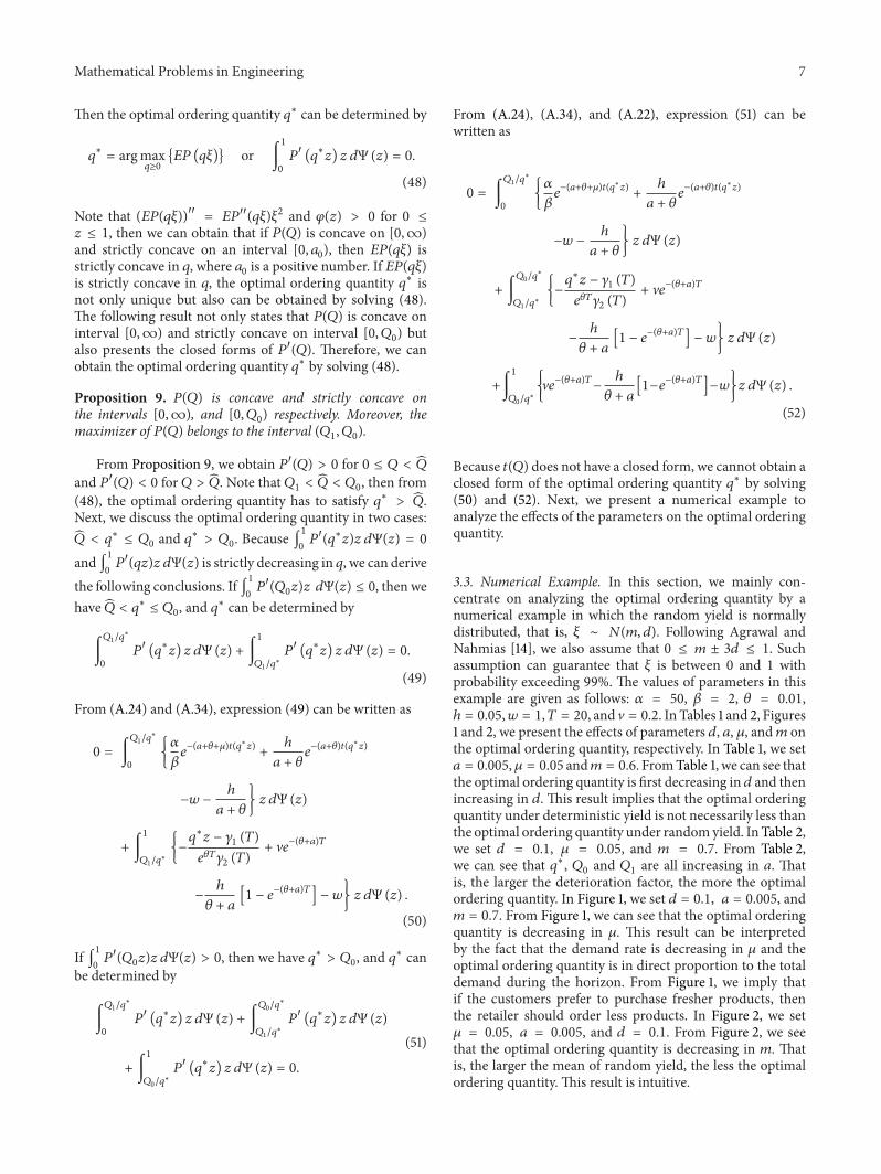
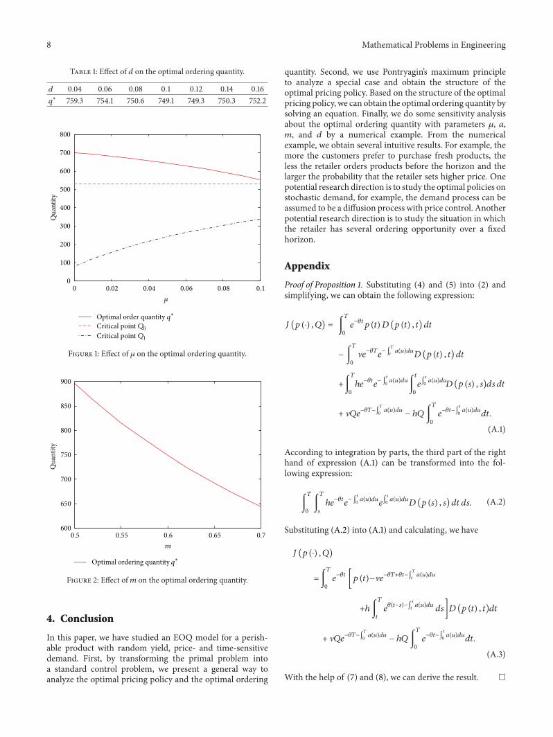
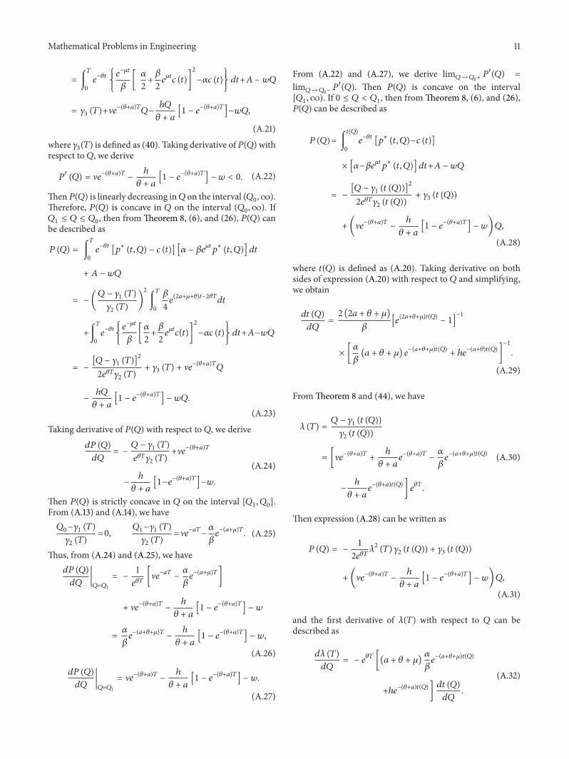


![A compound Poisson EOQ model for perishable items with ... › ws › files › 3620311 › 749511.pdf · uid EOQ model that was studied in [4]. Actually, both the uid EOQ model of](https://img.pdfslide.net/doc/110x75/5f0e5b927e708231d43edafd/a-compound-poisson-eoq-model-for-perishable-items-with-a-ws-a-files-a.jpg)