RESEARCH ARTICLE Controlling Aliased Dynamics in … · RESEARCH ARTICLE Controlling Aliased Dynamics in Motion Systems? ... Garnier and Wang 2008, Pintelon and Schoukens 1997)

21/11/2013 14:30 International Journal of Control Paper˙IJC˙2013˙V010˙final

International Journal of ControlVol. 00, No. 00, Month 200x, 1–25

RESEARCH ARTICLE

Controlling Aliased Dynamics in Motion Systems?

An Identification for Sampled-Data Control Approach

Tom Oomena∗

aEindhoven University of Technology, Faculty of Mechanical Engineering, Control Systems Technology

Group, PO Box 513, Building GEM-Z 0.131, 5600MB Eindhoven, The Netherlands.(Received 00 Month 200x; final version received 00 Month 200x)

Sampled-data control systems occasionally exhibit aliased resonance phenomena within the control bandwidth.The aim of this paper is to investigate the aspect of these aliased dynamics with application to a high perfor-mance industrial nanopositioning machine. This necessitates a full sampled-data control design approach, sincethese aliased dynamics endanger both the at-sample performance and the intersample behavior. The proposedframework comprises both system identification and sampled-data control. In particular, the sampled-datacontrol objective necessitates models that encompass the intersample behaviour, i.e., ideally continuous timemodels. Application of the proposed approach on an industrial wafer stage system provides a thorough insightand new control design guidelines for controlling aliased dynamics.

Keywords: Aliased dynamics, Continuous time system identification, Sampled-data control, Intersamplebehaviour, motion systems, mechatronics

1 Introduction

Despite the fact that modern control systems are generally implemented in a digital computerenvironment, the majority of such control sampled-data control systems are still being designedusing approximations. These approximations deteriorate the achieved control performance. Twodistinct approximate schemes can be roughly distinguished. In the first approach, a continuoustime controller is designed for the continuous time system. The designed controller is then ap-proximated by a discrete time controller for actual implementation. In the second approach, adiscrete time model is constructed (either by discretising a continuous time model or identifyinga discrete time system directly), followed by the design of a discrete time controller. The ap-proximation in the second approach arises from ignoring the intersample behavior. Indeed, theperformance of sampled-data control systems should generally be evaluated in the continuoustime domain. In this respect, good discrete time performance only provides a necessary conditionfor good sampled-data performance, since it is not sufficient.

For feedback controlled systems with relatively high sampling frequencies, the approximationerror can often be made negligible. However, there are important examples of high performancesystems and control design methodologies where the approximation error is very large and leadsto a severe deterioration of control performance. Examples include high-precision positioningsystems (Oomen et al. 2007), repetitive control (Hara et al. 1990), and iterative learning controltechniques, which are able to attenuate disturbances up to the Nyquist frequency (LeVoci andLongman 2004, Oomen et al. 2009).

The design of sampled-data controllers leads to several phenomena that are not encounteredin traditional continuous time or discrete time control designs, including

i) sampling zeros,

∗Corresponding author. Email: [email protected]

ISSN: 0020-7179 print/ISSN 1366-5820 onlinec© 200x Taylor & FrancisDOI: 10.1080/0020717YYxxxxxxxxhttp://www.informaworld.com


2 T. Oomen

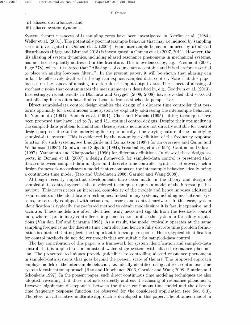
ii) aliased disturbances, andiii) aliased system dynamics.

System theoretic aspects of i) sampling zeros have been investigated in Astrom et al. (1984),Weller et al. (2001). The potentially poor intersample behavior that may be induced by samplingzeros is investigated in Oomen et al. (2009). Poor intersample behavior induced by ii) aliaseddisturbances (Riggs and Bitmead 2013) is investigated in Oomen et al. (2007, 2011). However, theiii) aliasing of system dynamics, including aliased resonance phenomena in mechanical systems,has not been explicitly addressed in the literature. This is evidenced by, e.g., Preumont (2004,Page 278), where it is stated that ”Aliasing is of course not acceptable and it is therefore essentialto place an analog low-pass filter...”. In the present paper, it will be shown that aliasing canin fact be effectively dealt with through an explicit sampled-data control. Note that this paperfocuses on the aspect of aliasing in deterministic input-output data. The aspect of aliasing ofstochastic noise that contaminates the measurements is described in, e.g., Goodwin et al. (2013).Interestingly, recent results in B lachuta and Grygiel (2009, 2008) have revealed that classicalanti-aliasing filters often have limited benefits from a stochastic perspective.

Direct sampled-data control design enables the design of a discrete time controller that per-forms optimally for a continuous time system by explicitly addressing the intersample behavior.In Yamamoto (1994), Bamieh et al. (1991), Chen and Francis (1995), lifting techniques havebeen proposed that have lead to H2 and H∞ optimal control designs. Despite their optimality inthe sampled-data problem formulation, these systems norms are not directly suitable for controldesign purposes due to the underlying linear periodically time-varying nature of the underlyingsampled-data system. This is evidenced by the non-unique definition of the frequency responsefunction for such systems, see Lindgarde and Lennartson (1997) for an overview and Quinn andWilliamson (1985), Goodwin and Salgado (1994), Freudenberg et al. (1995), Cantoni and Glover(1997), Yamamoto and Khargonekar (1996) for different definitions. In view of these design as-pects, in Oomen et al. (2007) a design framework for sampled-data control is presented thatiterates between sampled-data analysis and discrete time controller synthesis. However, such adesign framework necessitates a model that encompasses the intersample behavior, ideally beinga continuous time model (Rao and Unbehauen 2006, Garnier and Wang 2008).

Although recently important developments have been made in the theory and design ofsampled-data control systems, the developed techniques require a model of the intersample be-haviour. This necessitates an increased complexity of the models and hence imposes additionalrequirements on the identification techniques. Indeed, many systems, including mechatronic sys-tems, are already equipped with actuators, sensors, and control hardware. In this case, systemidentification is typically the preferred method to obtain models since it is fast, inexpensive, andaccurate. These models are often identified using measured signals from the feedback controlloop, where a preliminary controller is implemented to stabilize the system or for safety regula-tions (Van den Hof and Schrama 1995). As a result, the model typically operates at the samesampling frequency as the discrete time controller and hence a fully discrete time problem formu-lation is obtained that neglects the important intersample response. Hence, typical identificationfor control methods do not deliver models that are suitable for sampled-data control.

The key contribution of this paper is a framework for system identification and sampled-datacontrol that is applied to an industrial wafer stage system with aliased resonance phenom-ena. The presented techniques provide guidelines to controlling aliased resonance phenomenain sampled-data systems that goes beyond the present state of the art. The proposed epproachemploys models of the intersample behavior, i.e., ideally identified using a direct continuous timesystem identification approach (Rao and Unbehauen 2006, Garnier and Wang 2008, Pintelon andSchoukens 1997). In the present paper, such direct continuous time modeling techniques are alsoadopted, revealing that these methods correctly address the aliasing of resonance phenomena.However, significant discrepancies between the direct continuous time model and the discretetime frequency response function are observed for the considered application (see Sec. 6.3).Therefore, an alternative multirate approach is developed in this paper. The obtained model in


International Journal of Control 3

Cl Hl SlPr y

−Sl

ψluνlP l

Figure 1. Sampled-data feedback interconnection.

the multirate approach enhances correspondence to the slow sampled discrete time frequencyresponse function, at the expense of a reduced resolution in the intersample response. Note thatpresented sampled-data control framework can be extended straightforwardly for use with directcontinuous time identification methods.

Throughout, tc ∈ R denotes continuous time, whereas t ∈ Z denotes discrete time. Continuoustime signals are indicated by solid lines, whereas discrete time signals with sampling frequencyf l and fh are indicated by dashed and dotted lines, respectively. Here, fh = 1

hh = Ff l, F ∈ N,

and hh denotes sampling time. In addition, ωh = 2πfh. Similarly, hl := 1f l and ωl = 2πf l.

Throughout, it is assumed that sampling is non-pathological (Chen and Francis 1995, Definition3.2.1). Finally, to facilitate the presentation many results and examples are presented for SISOsystems. Generalisation to the multivariable situation is conceptually straightforward.

2 Case study: Aliasing of dynamics

2.1 General problem setting

Consider the setup in Fig. 1. Herein, P denotes the continuous time system. The ideal samplerS is defined by

S l : y(tc)→ ψl(t), ψl(ti) = y(tihl) (1)

In addition, the ideal zero-order-hold is defined by

Hl : νl(t)→ u(tc), u(tihl + τ) = νl(ti), τ = [0, hl). (2)

The discrete time system P l is given by

P l = S lPHl. (3)

It is emphasized that (3) is not an approximation of P in the sense that it represents the relationνl → ψl exactly at the sampling instants.

2.2 Motivating example

In many motion and vibration control applications, resonance phenomena in P endanger closed-loop stability of the system. A well-known solution to designing controllers for resonant systemsis by using so-called notch filters, see Preumont (2004, Sec. 4.5). Importantly, the design of suchnotch filters is often performed in continuous time (Preumont 2004, Sec. 4.5).

To introduce the concept of aliasing of resonance phenomena, the following example is con-sidered.

Example 2.1 Consider the continuous time system

P (s) =1

122 s2 + 2·0.02

2 s+ 1+ 0.5

1152 s2 + 2·0.01

5 s+ 1, (4)


4 T. Oomen

10−2

10−1

100

101

−50

−25

0

25

|P|[

dB]

fN

10−2

10−1

100

101

−180

−90

0

90

180

6(P

)[]

f [Hz]fN

Figure 2. Aliasing of resonance phenomena: continuous time system P (solid blue), and discretisation P l = SlPHl (dashedred) with Nyquist frequency fN . Note the aliased resonance in P l at f ≈ 2 · 10−1 Hz.

−0.1 −0.05 0 0.05 0.1

−8

−6

−4

−2

0

2

4

6

8

Continuous time s-plane

Real

Imag

−1 −0.5 0 0.5 1

−1

−0.5

0

0.5

1

Real

Imag

Discrete time z -plane

Figure 3. Aliasing of resonance phenomena: eigenvalues of A corresponding to continuous time system P (left), and eigen-values of Ad corresponding to discretisation P l = SlPHl (dashed red).

which is implemented in the setup of Fig. 1 with sampling time hl = 1. This leads to the systemP l in (3). Bode diagrams of the systems P and P l are depicted in Fig. 2. Interestingly, an aliasedresonance phenomenon appears at approximately 0.2 Hz that is not present in the underlyingcontinuous time system P at that particular frequency.

These observations are confirmed in Fig. 3, where the poles of P in (4) and P l in (3) areplotted. Note that the poles of P indicated by the diamond () appear at a higher frequencycompared to the ones indicated by a circle (). In contrast, after discretisation in view of (3),the poles of P l indicated with the diamond appear at a lower frequency. Indeed, the frequencyresponse of P (s) is obtained by substituting s = jω, whereas for P l(z) this is obtained by setting

z = ejωhl

.

Example 2.1 reveals that aliasing arises in systems under sampled-data control. Traditionalcontinuous time and discrete time control design only provide a partial perspective on the aspectof controlling these aliased dynamics:

• if a continuous time control design is pursued (based on either the frequency responsefunction of P or Pd in Fig. 2), it is not clear how to deal with the aliased resonance at 0.2Hz. Common guidelines include implementing anti-aliasing filters, e.g., Preumont (2004,Page 278). Note that the implementation of such filters is not always feasible in practice



and the use of anti-aliasing filters often leads to a phase delay that is disadvantageousfor achieving high control performance.

• if a discrete time control design is pursued, i.e., the direct design of a discrete timecontroller C l based on P l, then standard results on discrete time systems reveal that thealiased resonance should be taken into account in a similar manner as the other resonance.For instance, the discrete time Nyquist test resorts to the frequency response functionof Pd in Fig. 2. However, this only provides a partial and approximate result, sincethe intersample response is completely ignored. In fact, cases have been reported wherethe intersample behavior is extremely poor despite of a perfect at-sample performance(De Souza and Goodwin 1984, Hara et al. 1990, Oomen et al. 2007).

2.3 Problem formulation and outline

The key question that this paper aims to address is how to deal with these aliased resonance phe-nomena in sampled-data feedback systems. Addressing this question necessitates a full sampled-data framework, i.e., by analyzing the interconnection of the continuous time system P and thediscrete time controller C l.

This paper is organised as follows. In Sec. 3, the underlying mechanism of aliasing of systemdynamics in Example 2.1 is presented. Next, in Sec. 4, a framework for system identification forsampled-data control is presented. Next, the sampled-data control design framework is presentedin Sec. 5. The identification for sampled-data control framework is subsequently applied to acase study in Sec. 6 that addresses the aliasing of resonance phenomena in an industrial nano-positioning system. Finally, conclusions are presented in Sec. 7.

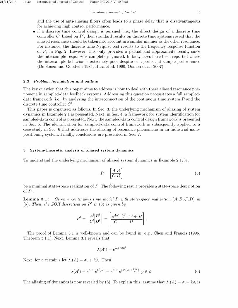
3 System-theoretic analysis of aliased system dynamics

To understand the underlying mechanism of aliased system dynamics in Example 2.1, let

P =

[A BC D

](5)

be a minimal state-space realization of P . The following result provides a state-space descriptionof P l.

Lemma 3.1: Given a continuous time model P with state-space realization (A,B,C,D) in(5). Then, the ZOH discretisation P l in (3) is given by

P l =

[Al Bl

C l Dl

]=

[eAh

l ∫ hl0 eτAdτB

C D

],

The proof of Lemma 3.1 is well-known and can be found in, e.g., Chen and Francis (1995,Theorem 3.1.1). Next, Lemma 3.1 reveals that

λ(Al) = eλi(A)hl

Next, for a certain i let λi(A) = σi + jωi. Then,

λ(Al) = ehlσieh

ljωi = ehlσiejh

l(ωi+2πp

hl), p ∈ Z. (6)

The aliasing of dynamics is now revealed by (6). To explain this, assume that λi(A) = σi+ jωi is


6 T. Oomen

an eigenvalue of A that is mapped to λi(Al). Then, all eigenvalues λk(A) = σk + jωk satisfying

σk = σi and ωk = ωi +2π

hlp, p ∈ Z

lead to λi(Al) = λk(A

l). Hence, the mapping from P to P l in (5) and Lemma 3.1 is not injectiveand no unique inverse exists.

Returning to Example 2.1 reveals that a minimal state-space realization (A,B,C,D) of P leadsto A ∈ R4×4. Next, the resulting eigenvalues of A, i.e., λi(A), i = 1, 2, 3, 4 exactly correspondto the poles of P in (5) and Fig. 3 (left). Note that indeed two of the eigenvalues are strictlyinside the primary frequency band, i.e., |=(λi)| < π

hl = π, whereas the other two eigenvalues areoutside the primary frequency band. Next, observe from (6) that the relation between values inthe primary frequency band (indicated in the left-hand plot of Fig. 3 by the magenta strip) mapuniquely onto the unit disc in the discrete time plane (the right-hand plot in Fig. 3). However,the higher frequency bands (indicated in the left-hand plot of Fig. 3 by the green strips) alsomap onto the unit disk. Since there are eigenvalues inside the green strip, aliasing occurs.

Hence, Lemma 3.1 provides insight in the mechanism of aliasing based on state-space realiza-tions. To connect this to the frequency response function results in Example 2.1, note that theFourier transforms of Ψl(ejωh

l

) of ψl and Y (jω) of y in (1) and Fig. 1 are related by (Chen andFrancis 1995, Lemma 3.3.1)

Ψl(ejωhl

) =1

hl

∞∑k=−∞

Y (jω − jωlk). (7)

In addition, the Fourier transforms U(jω) of u and N l(ejωhl

) of νl in (2) and Fig. 1 are relatedby (Chen and Francis 1995, Lemma 3.3.2)

U(jω) = Hl(jω)N l(ejωhl

), Hl(jω) =1− e−jωhl

jω(8)

The function Hl(jω) in (8) is illustrated in Fig. 4. The following result connects the frequency

response functions of P l(ejωhl

) and P (jω).

Lemma 3.2: The frequency response functions P l(ejωhl

) and P (jω) of the systems in Fig. 1are related by

P l(ejωhl

) =1

hl

∞∑k=−∞

P (jω − jωlk)Hl(jω − jωlk). (9)

Proof First, observe that P l(ejωhl

) = Ψl(ejωhl)

N l(ejωhl ). Next, note that Y (jω) = P (jω)U(jω) and

U(jω) = Hl(jω)N l(ejωhl

). Combining this with (7) immediately yields (9).

Lemma 9 reveals how aliasing occurs. In particular, note that if νl 6= 0, then u containsfrequency components outside of the primary frequency band, since N l(ejωh

l

) is periodic with

period 2πhl and |Hl(jω)| > 0 for ω > |ωl2 |. The continuous time system is thus excited at frequen-

cies ω > |ωl2 |. Since P is assumed LTI, the same frequency components are present in the outputy. These high-frequency components in y are subsequently observed in the primary frequencyband ω < |ωl2 | through (7). Thus, if P has a large amplification at high frequencies, e.g., due toa resonance frequency, then the result will be observed at lower frequencies.



|Hl |

0

T l

− 4ωs − 3ωs − 2ωs − ωs 0 ωs 2ωs 3ωs 4ωs

−180

−90

0

90

180

− 4ωs − 3ωs − 2ωs − ωs 0 ωs 2ωs 3ωs 4ωs

6(H

l )[]

ω [rad/s]

Figure 4. Frequency response Hl(jω) in (8).

4 Identification for sampled-data control

4.1 Problem setting: towards a multirate approach

The goal in this paper is to investigate the control design for system having aliased dynamics as isillustrated in Example 2.1. This investigation will be performed for an industrial nanopositioningsystem that immediately confirms practical relevance of the presented results. This necessitatesa full analysis that comprises both the at-sampled response, i.e., using sampled signals availableto the discrete time controller, and the intersample behavior. To address the full intersamplebehavior, such an approach requires a continuous time model of the system that has to beidentified. Although such a continuous time model is highly desirable for the approach in thispaper, an approximation is introduced to obtain a tractable and validatable approach, since

• measurement limitations prohibit the use of continuous time signals, e.g., for performancevalidation of the implemented controller. In this paper, a fast sampled process output willbe used to validate the results, as these signals are readily available for the consideredsystem.

• the identification of continuous time models, as is required by a full sampled-data con-trol design approach, is not straightforward for certain classes of systems, including theexperimental setup that is considered in this paper. Indeed, these systems generally havemany high-frequency resonance phenomena (Hughes 1987) and the modeling of suchsystems is commonly performed using an intermediate step of frequency domain systemidentification (Pintelon et al. 1994), as is also considered in the related applications inVan de Wal et al. (2002), De Callafon and Van den Hof (2001), Oomen et al. (2013).As a result, frequency domain approaches to continuous time system identification, seePintelon et al. (1994, 2000), Pintelon and Schoukens (2012) are considered.In a frequency domain formulation, a continuous time model can be identified directlyif band-limited excitation signals (Pintelon and Schoukens 2012) are employed or if ac-cess is available to the continuous time input and output and anti-aliasing filters can beimplemented (Pintelon and Schoukens 1997). This is only approximately the case in theconsidered experimental setup in Sec. 6, since all continuous time signals are constructedusing zero-order-hold interpolation and the implemented anti-aliasing filters will be in-sufficient to completely eliminate aliasing. This is further experimentally investigated inSec. 6.3.2.

In view of the above considerations, the experimental validation and control design will beperformed in a multirate setup. Therefore, the multirate control setup1 of Fig. 5 is consid-ered throughout, which constitutes the best approximation of the sampled-data control problemYamamoto (1994), Bamieh et al. (1991), Chen and Francis (1995) in view of measurement limita-tions. Herein, ωh and ζh denote all exogenous inputs and outputs, respectively, and are sampled

1The notation ω is used to represent both radial sampling frequencies and exogenous inputs, it follows from the contextwhich one is referred to.


8 T. Oomen

Gh

SdHu

Cl

ζhωh

ψhνh

ψlνl

Figure 5. Multirate standard plant setup.

Cl Hu PHh up

−Sd

ypνhpνlprSh

ρSdSh

ψhp

ψlp

ωh = Shr

−

ψh

ζh

νh

P l

Ph

Figure 6. Feedback interconnection of Fig. 1 in a multirate setting.

at the high sampling frequency fh. The measured output that is available for the controller isgiven by ψl and is sampled at the slow sampling frequency f l. In addition, the manipulatedcontrol input is given by νl and also operates at the low sampling frequency f l. The discretetime controller C l operates at the low sampling frequency f l, whereas the standard plant Gh

operates at the high sampling frequency fh. In addition, C l and Gh are interconnected throughthe downsampler

Sd : eh(t)→ el(t), el(ti) = eh(Fti), ti ∈ t. (10)

and multirate zero-order-hold

Hu = IF (z)Su,

where the upsampler Su and zero-order-hold interpolator IF (z) are given by

Su : ul(t)→ uh(t), uh(ti) :=

ul( tiF ) for ti

F ∈ Z0 for ti

F /∈ Z.(11)

IF (z) =

F−1∑f=0

z−f , (12)

see also Oomen et al. (2007) for more details.Note that the setup of Fig. 5 encompasses common control structures, including the feedback

interconnection in Fig. 1. This is illustrated in Fig. 6, where all signals corresponding to Fig. 5are indicated. Here, Gh contains a model P h = ShPHu. This motivates the identification of afast sampled system. It is emphasized that the results in this paper apply equally to the sampled-data case, i.e., if the exogenous input ωh and output ζh are continuous time signals. In fact, thesampled-data setup is recovered if hh → 0.



4.2 System identification approach

The key idea in this paper is to identify the model P h using measured data obtained at thesampling frequency fh. This is indeed feasible in many practical applications, where the samplingfrequency f l is upper bounded due to the constraint that the feedback controller has to computea new control input in real time. In contrast, in many control applications it is possible tomeasure and store the error signal at a higher sampling frequency fh, or implement a low-complexity controller that requires less computational effort and thus can be implemented at ahigh sampling frequency fh. As a result, the measured signals at the high sampling frequencycan be processed off-line by the identification algorithm.

The approach to identify P h consists of two steps.

i) Identify a frequency response function of P ho (zi) at sampling frequency fh, zi = ejωihh

. Thiswill be described in detail in Sec. 6.2, see also Pintelon and Schoukens (2012) for furtherbackground information.

ii) Next, a parametric model is estimated using the criterion

J(θ) =

N∑i=1

∥∥∥Wi

(Po(zi)− P (zi, θ)

)∥∥∥2

2, (13)

where Wi denotes a user-chosen weighting, and provides freedom to identify e.g. a maximum-likelihood estimate (Pintelon and Schoukens 2012) or a control-relevant model (Schrama1992, Gevers 1993, Oomen and Bosgra 2012, Oomen et al. 2013). See also De Callafon et al.(1996) for multivariable extensions. The model is parameterized as

P (z, θ) =b(z, θ)

a(z, θ)=bnbz

nb + bnb−1znb−1 + . . .+ b0

zna + ana−1zna−1 + . . .+ b0,

where na denotes the order and nb = na for a bi-proper model. The actual minimisation of(13) is then performed using the algorithm in, e.g., Oomen and Steinbuch (2014)

The result of this two-step procedure is a model P h that is suitable for control design. Theaspect of controller design is investigated next.

Remark 1 : In the case where an anti-aliasing filter GAA is implemented before the samplerS, then this is automatically incorporated in the model as ShGAAPHh. The resulting procedureautomatically takes this into account. However, such a direct implementation of an anti-aliasingfilter cannot eliminate the aspect of aliasing completely and often comes at the expense of aphase delay. Note that besides the input-output dynamics ShGAAPHh, the anti-aliasing filterGAA also affects the noise characteristics before sampling, see Goodwin et al. (2013), B lachutaand Grygiel (2009, 2008). Furthermore, the introduction of phase delay by anti-aliasing filter canbe avoided by more general implementations, see Goodwin et al. (2013), Delgado et al. (2011).

5 Sampled-data control design: A frequency domain multirate approach

In Sec. 4.2, an approach to identify a model P h is estimated that will be an essential part of thegeneralised plant Gh in Fig. 5. In this section, the standard plant Gh will be further completedby specifying control design objectives. The controller design for many systems, including theexperimental setup in Fig. 6, is performed in the frequency domain. Such controller designscan be either based on manual tuning, e.g., loop-shaping design of PID controllers, or usingoptimization algorithms, e.g., H∞-optimization. Note that frequency domain controller designscan equally well be done in the continuous time and discrete time domain, see Oomen et al.(2007). However, for the sampled-data and multi-rate setup of Fig. 5, pursuing a frequency


10 T. Oomen

domain approach is not straightforward. This is investigated in detail next, followed by a controldesign procedure.

5.1 The setup in Fig. 5 is LPTV

The key aspect in controller design for the setup of Fig. 5 is the fact that the notion of frequencyresponse function is not defined uniquely. This is confirmed by the following lemma.

Lemma 5.1: Let ωh in Fig. 5 have discrete time Fourier transform Ωh(ejωhh

). Then, ζh hasa discrete time Fourier transform given by

Zh(ejωhh

) =Gh11(ejωhh

)Ωh(ejωhh

)

+Gh12(ejωhh

)IZOH(ejωhh

)Ql(ejωhl

)

1

F

F−1∑f=0

Gh21(ejhh(ω− f

Fωh))Ωh(ejh

h(ω− f

Fωh))

(14)

where

Ql(ejωhl

) = (I − C l(ejωhl)Gl22(ejωhl

))−1C l(ejωhl

) (15)

and Gl22 = SdGh22Hu as in Lemma 6.1 and Gh is partitioned appropriately, i.e.,

Gh =

(Gh11 G

h12

Gh21 Gh22

).

Proof The result (14) follows directly from the fact that the Fourier transforms corresponding

to (10) is given byEl(ejωhl

) = 1F

∑F−1f=0 E

h(ejhh(ω− f

Fωh)). In addition, the Fourier transform

corresponding to (11) is given by Uh(ejωhh

) = U(ejωhl

). Finally, (12) is used.

Lemma 5.1 reveals that the setup in Fig. 5 has significantly different properties compared tostandard discrete time or continuous time system interconnections. To see this, note that appli-cation of a single sinusoid in (14) reveals that Zh(ejωh

h

) contains multiple frequency components.This is due to the fact that the multirate system Ll(Gh,HuC lSd) in Fig. 5 is linear periodicallytime varying (LPTV). In the next section, new notions for frequency response functions for thesetup of Fig. 5 are presented.

5.2 Frequency response functions for sampled-data systems

Lemma 5.1 reveals that the multirate setup in Fig. 5 is LPTV and hence the notion of frequencyresponse function, as is defined for LTI systems, does not directly apply. In fact, several gen-eralisations of frequency response functions for the setup of Fig. 5 can be defined. The signalspaces

WD =w(t)

∣∣∣w(t) = cejωhht, ‖c‖2 <∞

WMR =

w(t)

∣∣∣∣∣∣w(t) =

F−1∑f=0

cfej(ω−fωh)hht, ‖cf‖2 <∞



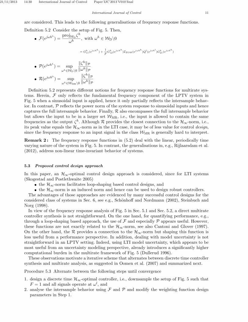
are considered. This leads to the following generalisations of frequency response functions.

Definition 5.2 Consider the setup of Fig. 5. Then,

• F(ejωhh

) =projWD

ζh

ωh, with ωh ∈ WD\0

= Gh11(e

jωhh) +

1

FGh12(e

jωhh)IZOH(e

jωhh)Q

l(ejωhl

)Gh21(e

jωhh)

• P(ejωhh

) = supωh∈WD\0

‖ζh‖P‖ωh‖P

• R(ejωhh

) = supωh∈WMR\0

‖ζh‖P‖ωh‖P

Definition 5.2 represents different notions for frequency response functions for multirate sys-tems. Herein, F only reflects the fundamental frequency component of the LPTV system inFig. 5 when a sinusoidal input is applied, hence it only partially reflects the intersample behav-ior. In contrast, P reflects the power norm of the system response to sinusoidal inputs and hencecaptures the full intersample behavior. Finally, R also encompasses the full intersample behaviorbut allows the input to be in a larger set WMR, i.e., the input is allowed to contain the samefrequencies as the output ζh. Although R provides the closest connection to the H∞-norm, i.e.,its peak value equals the H∞-norm as in the LTI case, it may be of less value for control design,since the frequency response to an input signal in the class WMR is generally hard to interpret.

Remark 2 : The frequency response functions in (5.2) deal with the linear, periodically timevarying nature of the system in Fig. 5. In contrast, the generalisations in, e.g., Rijlaarsdam et al.(2012), address non-linear time-invariant behavior of systems.

5.3 Proposed control design approach

In this paper, an H∞-optimal control design approach is considered, since for LTI systems(Skogestad and Postlethwaite 2005)

• the H∞-norm facilitates loop-shaping based control designs, and

• the H∞-norm is an induced norm and hence can be used to design robust controllers.The advantages of those approaches are evidenced by many successful control designs for the

considered class of systems in Sec. 6, see e.g., Schonhoff and Nordmann (2002), Steinbuch andNorg (1998).

In view of the frequency response analysis of Fig. 5 in Sec. 5.1 and Sec. 5.2, a direct multiratecontroller synthesis is not straightforward. On the one hand, for quantifying performance, e.g.,through a loop-shaping based approach, the use of F and especially P appears useful. However,these functions are not exactly related to the H∞-norm, see also Cantoni and Glover (1997).On the other hand, the R provides a connection to the H∞-norm but shaping this function isless useful from a performance perspective. In addition, dealing with model uncertainty is notstraightforward in an LPTV setting. Indeed, using LTI model uncertainty, which appears to bemost useful from an uncertainty modeling perspective, already introduces a significantly highercomputational burden in the multirate framework of Fig. 5 (Dullerud 1996).

These observations motivate a iterative scheme that alternates between discrete time controllersynthesis and multirate analysis, as suggested in Oomen et al. (2007) and summarized next.

Procedure 5.3 Alternate between the following steps until convergence

1. design a discrete time H∞-optimal controller, i.e., downsample the setup of Fig. 5 such thatF = 1 and all signals operate at ωl, and

2. analyse the intersample behavior using F and P and modify the weighting function designparameters in Step 1.


12 T. Oomen

In Step 1, a downsampled model of P h is used, i.e., P l = SdP hHu, see also Lemma 6.1. Inthis case, all functions F , P, and R are equal and hence (14) becomes the standard frequencyresponse function for discrete time systems. In contrast, the intersample analysis in Step 2 resortsto a model P h. Note that if the intersample behavior is not satisfactory in Step 2, the weightingfunction design parameters regarding the function Ql in (15) should be adjusted in Step 1.

Procedure 5.3 is employed in the forthcoming sections to design a controller that deals withaliased resonance phenomena. First, the modeling of P h and hence P l is considered, since thesemodels are required for Procedure 5.3.

6 Application to controlling aliased resonance phenomena of a wafer stage

6.1 Experimental setup

The considered experimental setup in this paper is a wafer stage, see Fig. 7. Wafer stages arenano-positioning systems that are used in semiconductor manufacturing. These systems arecontrolled in all six motion degrees-of-freedom (i.e., three rotations and three translations), andhave an operating range in the order of 1 m in the horizontal plane, and a typical accuracy inthe order of 1 nm. This is achieved by laser interferometers that have sub-nanometer accuracy,in conjunction with a moving coil permanent magnet planar motor that provides contactlessoperation (Oomen et al. 2013). Due to the high accuracy of the laser interferometers, almost nopre-processing is done in the sense of anti-aliasing filters. Indeed, common implementations ofsuch filters generally lead to phase lag.

The controller C l that will be designed in this section operates at a sampling frequency of f l =1 kHz. In contrast, since identification can be performed off-line and does not impose any real-time computational requirements, this can be performed at much higher sampling frequencies.In the used software implementation, it is possible to identify P h at a sampling frequency offh = 5 kHz, hence F = 5.

To investigate the aspect of controlling aliased dynamics, attention is restricted to the verticaltranslational direction, i.e., the identification and control design will be done for a SISO system.The remaining degrees-of-freedom are controlled using low-performance PID controllers. For aMIMO control design along the same lines, the reader is referred to Oomen et al. (2013). Inthe MIMO case, a high performance controller is designed for all six motion degrees-of-freedom,which is significantly more complex during both system identification and control design. In-deed, the resonance phenomena are inherently multivariable. This implies that a direct multi-variable model has to be estimated, which is numerically and computationally significantly morechallenging. Furthermore, the multivariable resonance phenomena have to be controlled usinga multivariable controller, which significantly increases the complexity during the design andpossible uncertainty modeling.

6.2 Frequency response identification: aliasing of dynamics

The first step in the system identification procedure is the identification of a frequency responsefunction. Two frequency response functions are identified, both at the low sampling frequency f l

and at the high sampling frequency fh. An external excitation φ is applied at the system input,see Fig. 8 for the case with f l. The measured signals are νl and ψl. Despite the advantages ofperiodic input signals (Pintelon and Schoukens 2012, Chapter 2), the signal φ is automaticallyselected in the industrial application as a realization of a stochastic process, being normallydistributed white noise. Next, frequency response function estimates of the closed-loop transferfunctions [

P lSl

Sl

]=

[P l(1 + C lP l)−1

(1 + C lP l)−1

]



Figure 7. Photograph of the experimental setup.

Cl P lρ

ψl

−

νlφl

Figure 8. System identification setup.

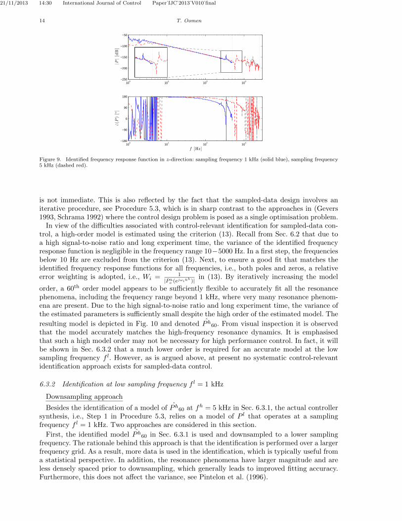
are computed using spectral analysis, see, e.g., Ljung (1999, Section 6.4). It is well-known thatthese are essentially open-loop identification problems, since ψ is noise-free. Since abundantdata is available with large signal-to-noise ratio, frequency response function estimates withvery small bias and variance are obtained. Next, a frequency response estimate of P l is obtainedby performing the division (P lSl)(Sl)−1. An analogous approach is applied for P h. The resultsare depicted in Fig. 9. Note that these results correspond to the systems P l and P h in Fig. 6,respectively.

Inspection of Fig. 9 confirms that the influence of noise on the estimated frequency responsefunction is small in the frequency range 10 − 5000 Hz. Below 10 Hz, the influence of the noiseis large due to the fact that Sl has a small magnitude at low frequencies. This induces errorsin the estimation of P l due to the presence of a feedback controller, as is explained in detail inHeath (2001) and Pintelon and Schoukens (2001).

When comparing the results in Fig. 9, it appears that the 1 kHz identification contains aresonance phenomenon around 347 Hz. Interestingly, the identification result at 5 kHz does notcontain a resonance phenomenon at 347 Hz. Instead, it contains a resonance at 653 Hz that’folds’ around the Nyquist frequency of 500 Hz. Hence, the identified result at 1 kHz containsaliased dynamics, which clearly resembles the situation in Example 2.1.

6.3 Parametric identification for sampled-data control

6.3.1 Identification at high sampling frequency fh = 5 kHz

The sampled-data approach pursued in this paper necessitates a fast sampled model at 5 kHzto investigate the intersample behavior. Visual inspection of the frequency response function inFig. 9 reveals the presence of many resonance phenomena. In fact, more resonance phenomenawill become visible as the sampling frequency increases (Hughes 1987). Recent research (Oomenet al. 2013) has revealed that only a small number of resonance phenomena are relevant forcontrol design. If a control-relevant identification criterion is formulated (Gevers 1993, Schrama1992), then the identification approach automatically selects these dynamics and incorporatesthese in the identified model. However, in view of Lemma 5.1, the sampled-data system is LPTV.Hence, posing and solving a control-relevant identification criterion for sampled-data systems


14 T. Oomen

100

101

102

103

−250

−200

−150

−100

−50

|P|[

dB]

100

101

102

103

−180

−90

0

90

180

6(P

)[]

f [Hz]

Figure 9. Identified frequency response function in z-direction: sampling frequency 1 kHz (solid blue), sampling frequency5 kHz (dashed red).

is not immediate. This is also reflected by the fact that the sampled-data design involves aniterative procedure, see Procedure 5.3, which is in sharp contrast to the approaches in (Gevers1993, Schrama 1992) where the control design problem is posed as a single optimisation problem.

In view of the difficulties associated with control-relevant identification for sampled-data con-trol, a high-order model is estimated using the criterion (13). Recall from Sec. 6.2 that due toa high signal-to-noise ratio and long experiment time, the variance of the identified frequencyresponse function is negligible in the frequency range 10−5000 Hz. In a first step, the frequenciesbelow 10 Hz are excluded from the criterion (13). Next, to ensure a good fit that matches theidentified frequency response functions for all frequencies, i.e., both poles and zeros, a relativeerror weighting is adopted, i.e., Wi = 1

|Pho (ejωihh )| in (13). By iteratively increasing the model

order, a 60th order model appears to be sufficiently flexible to accurately fit all the resonancephenomena, including the frequency range beyond 1 kHz, where very many resonance phenom-ena are present. Due to the high signal-to-noise ratio and long experiment time, the variance ofthe estimated parameters is sufficiently small despite the high order of the estimated model. The

resulting model is depicted in Fig. 10 and denoted P h60. From visual inspection it is observedthat the model accurately matches the high-frequency resonance dynamics. It is emphasisedthat such a high model order may not be necessary for high performance control. In fact, it willbe shown in Sec. 6.3.2 that a much lower order is required for an accurate model at the lowsampling frequency f l. However, as is argued above, at present no systematic control-relevantidentification approach exists for sampled-data control.

6.3.2 Identification at low sampling frequency f l = 1 kHz

Downsampling approach

Besides the identification of a model of P h60 at fh = 5 kHz in Sec. 6.3.1, the actual controllersynthesis, i.e., Step 1 in Procedure 5.3, relies on a model of P l that operates at a samplingfrequency f l = 1 kHz. Two approaches are considered in this section.

First, the identified model P h60 in Sec. 6.3.1 is used and downsampled to a lower samplingfrequency. The rationale behind this approach is that the identification is performed over a largerfrequency grid. As a result, more data is used in the identification, which is typically useful froma statistical perspective. In addition, the resonance phenomena have larger magnitude and areless densely spaced prior to downsampling, which generally leads to improved fitting accuracy.Furthermore, this does not affect the variance, see Pintelon et al. (1996).



100

101

102

103

−250

−200

−150

−100

−50

|Ph|[

dB]

100

101

102

103

−180

−90

0

90

180

6(P

h)[]

f [Hz]

Figure 10. Identified frequency response function in z-direction (solid blue) and identified 60th order model Ph60 (dashed

red). Both models have sampling frequency 5 kHz.

Lemma 6.1: Let a model P h operate at sampling frequency fh and have state space realization

P h =

[Ah Bh

Ch Dh

].

Then a state-space realization of the downsampled system P l, see Fig. 6 and (3), is given by[Al Bl

? ?

]=

[Apd,h B

pd,h

0 I

]F,

[CpdDpd

]=

[Cpd,hDpd,h

],

where ? denotes a matrix entry that is not used in further computations.

Proof Follows directly from successive substitution of the state equation ξh(t+ 1) = Ahξh(t) +Bhνh(t) and νh(t+ f) = νl( tF ), f = 0, . . . , F − 1.

Lemma 6.1 is applied to the model P h60, leading to a 60th order model denoted P l60. The

results are depicted in Fig. 11. Interestingly, the downsampled model P l60 also has a resonance

at approximately 349 Hz that was not present in the original model P h60. Hence, Lemma 6.1takes sampling of system dynamics into account as is required.

Direct continuous time approachUnfortunately, the fit of the aliased resonance is less accurately modeled at sampling frequency

f l when compared to the original model P h60, as can clearly be observed from Fig. 11. A possi-ble explanation is that the system exhibits small parasitic nonlinear effects. Indeed, note that ifthe discrete time frequency response function P l is identified, a signal νl in Fig. 6 is generated.This signal is constructed using Hl in Fig. 6. The frequency response of Hl resembles the Bodediagram in Fig. 4. Hence, high-frequency components are reduced in amplitude when comparedto the direct excitation at the sampling frequency fh. Interestingly, in Smith (1998), similarobservations have been reported in a comparison between open-loop and closed-loop identifica-tion of a related system. Note that an LTI anti-aliasing filter has not caused the discrepancy inFig. 11, since from an identification perspective the anti-aliasing filter is identified as part of theLTI system.

To further investigate (1) the discrepancy in Fig. 11, and (2) the high model order equal to60, a direct continuous time approach is adopted. Here, a frequency domain continuous timeidentification approach is employed, where a frequency response function with band-limitedexcitation signals is approximated. The resulting frequency response function is depicted in


16 T. Oomen

100

101

102

103

−200

−150

−100

−50

|Pl |[dB]

346.5 349

100

101

102

103

−180

−90

0

90

180

6(P

l )[]

f [Hz]

Figure 11. Identified frequency response function in z-direction (solid blue), downsampled 60th order model P l60 (dashed

red), and identified 6th order model P l6 (dash-dotted green). All models have sampling frequency 1 kHz.

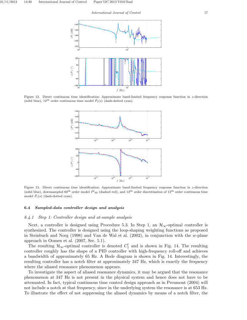
Fig. 12. Notice the large difference in phase when comparing these results to Fig. 10. Next, a12th order continuous time model P (s) is identified that fits the dominant resonance phenomena.These resonance phenomena are the physical resonance modes and are known to contain noaliasing phenomena. The identified 12th order continuous time model P (s) is extended by acomputational delay of 1.6 · 10−4 s, which has been identified separately, see also Pintelon andSchoukens (2012, Section 8.5) for details. The discretised model at f l = 1 kHz that includes

the computational delay is finite dimensional and of 13th order, see Astrom and Wittenmark(1990, Sec. 3.2) for an explanation on the resulting model order. The resulting discretised modelis depicted in Fig. 13.

The following conclusions are drawn from the resulting discretised model in Fig. 13. First,the direct continuous time approach correctly predicts the aliasing of resonance phenomenaand results in a slightly better fit of the resonance at approximately 349 Hz. However, theimprovement compared to the results using the downsampling approach in Fig. 11 is onlymarginal. Note that this aliased resonance phenomenon is of key importance, since it clearlyendangers stability as is shown in Fig. 15 in Sec. 6.4.1. Note also that the continuous timefit is less accurate in other frequency ranges and misses several other resonance phenomenawhen compared to the 60th order model in Fig. 11. Partially, this is caused by a significantlylower order of the model. Although alternative direct continuous time models may significantlyenhance the quality, the aim in the present paper is to investigate the role of aliased resonancephenomena. Therefore, for analysing the intersample behavior, the 60th order in Fig. 11 is used.Next, a discrete time approach is investigated for obtaining an accurate model for controllersynthesis.

Discrete time identificationMotivated by the discrepancy in Fig. 11 and Fig. 13, and the relatively high order of the

model P l60, a second approach is pursued to obtain a model of P l. Herein, the identificationapproach in Sec. 4.2 is used to directly fit a model to the identified frequency response functionat f l = 1 kHz in Fig. 11. The resulting 6th order model is also depicted in Fig. 11 and is denoted

P l6. From visual inspection of 11, it appears that the model P l6 is a significantly better fit of

the aliased resonance phenomenon at 347 Hz compared to the model P h60.



102

103

−220

−200

−180

−160

−140

|P|[d

B]

102

103

−180

−90

0

90

180

6(P)[]

f [Hz ]

Figure 12. Direct continuous time identification: Approximate band-limited frequency response function in z-direction

(solid blue), 12th order continuous time model Pc(s) (dash-dotted cyan).

102.4

102.5

102.6

102.7

−180

−170

−160

−150

−140

−130

|Pl |[dB]

102.4

102.5

102.6

102.7

−180

−90

0

90

180

6(P

l )[]

f [Hz ]

Figure 13. Direct continuous time identification: Approximate band-limited frequency response function in z-direction

(solid blue), downsampled 60th order model P l60 (dashed red), and 13th order discretisation of 12th order continuous time

model Pc(s) (dash-dotted cyan).

6.4 Sampled-data controller design and analysis

6.4.1 Step 1: Controller design and at-sample analysis

Next, a controller is designed using Procedure 5.3. In Step 1, an H∞-optimal controller issynthesized. The controller is designed using the loop-shaping weighting functions as proposedin Steinbuch and Norg (1998) and Van de Wal et al. (2002), in conjunction with the w-planeapproach in Oomen et al. (2007, Sec. 5.1).

The resulting H∞-optimal controller is denoted C l1 and is shown in Fig. 14. The resultingcontroller roughly has the shape of a PID controller with high-frequency roll-off and achievesa bandwidth of approximately 65 Hz. A Bode diagram is shown in Fig. 14. Interestingly, theresulting controller has a notch filter at approximately 347 Hz, which is exactly the frequencywhere the aliased resonance phenomenon appears.

To investigate the aspect of aliased resonance dynamics, it may be argued that the resonancephenomenon at 347 Hz is not present in the physical system and hence does not have to beattenuated. In fact, typical continuous time control design approach as in Preumont (2004) willnot include a notch at that frequency, since in the underlying system the resonance is at 653 Hz.To illustrate the effect of not suppressing the aliased dynamics by means of a notch filter, the


18 T. Oomen

100

101

102

103

100

110

120

130

140

150

|Cl |[dB]

100

101

102

103

−180

−90

0

90

180

6(C

l )[]

f [Hz]

Figure 14. Controller Cl1 (H∞-optimal controller) (solid blue), Controller Cl

2 (H∞-optimal controller with notch filterremoved) (dashed red). Both controllers have sampling frequency 1 kHz.

−2 −1.5 −1 −0.5 0 0.5 1 1.5 2−2

−1.5

−1

−0.5

0

0.5

1

1.5

2

Real(P l6C

l)

Imag(P

l 6C

l )

Figure 15. Nyquist diagram corresponding to loop-gain PC with Controller Cl1 (solid blue), and Cl

2 (dashed red). Allmodels and controllers have sampling frequency 1 kHz.

local notch filter is removed using a modal reduction technique. The resulting controller is calledC l2 and is depicted in Fig. 14.

An discrete time analysis, i.e., solely at the sampling frequency f l leads to the Nyquist di-agram of the loop-gains in Fig. 15. Interestingly, both controllers have a phase margin of 29.However, the gain margin reduces from 7.58 dB for C l1 to 0.593 dB for C l2. This implies poorrobustness properties for C l2. These observations are corroborated by the sensitivity function

1

1+P l6Cin Fig. 16, revealing a large peak for C l2, implying a poor modulus margin. In addition,

the sensitivity function exactly describes the at-sample performance. This implies that controllerC l2 is already expected to have a significantly worse at-sample behaviour compared to C l1. Fi-

nally, the process sensitivity functions P l61+P l6C

are depicted in Fig. 18. These results confirm the

earlier conclusions in the sense that C l2 leads to worse at-sample attenuation of disturbances atthe system input when compared to C l1. However, these observations do not provide any guaran-tees whether C l1 actually leads to better performance, since the intersample behaviour has beencompletely ignored so far.



100

101

102

103

−80

−60

−40

−20

0

20

|1

1+P

l 6C

l|[dB]

f [Hz]

Figure 16. Bode magnitude diagram corresponding to Sensitivity function 1

1+P l6Cl1

(solid blue), and 1

1+P l6Cl2

(dashed

red). All models and controllers have sampling frequency 1 kHz.

Ph

−

Sd

Cl

Hu

ωh ζhGh

Figure 17. Setup for computation of P in Definition 5.2.

100

101

102

103

−220

−210

−200

−190

−180

−170

−160

−150

−140

−130

−120

|.|[dB]

f [Hz]

Figure 18. Intersample analysis: P (see Definition 5.2) with Cl1 (solid blue), P with Cl

2 (dashed red).

6.4.2 Step 2: Intersample analysis

The controllers designed in Sec. 6.4.1 have been designed at a sampling frequency f l, therebycompletely ignoring the intersample behaviour. This step is of crucial importance, since severalcases have been reported (see Sec. 1) where controllers deteriorate the performance despite ofan almost perfect at-sample response. Therefore, Step 2 in Procedure 5.3 is performed.

To anticipate on the experiments that will be performed in Sec. 6.5, the function P is computedusing the setup in Fig. 17. In particular, the reference signal is set to zero and disturbances onthe fast sampled system input are considered. The exogenous output is selected as the systemoutput ψh.


20 T. Oomen

0 0.005 0.01 0.015 0.02 0.025−3

−2

−1

0

1

2

3x 10

−8

error[m

]

0 0.005 0.01 0.015 0.02 0.025−3

−2

−1

0

1

2

3x 10

−8

t [s]

error[m

]

Figure 19. Measured error signals: at low sampling frequency (solid blue) and at high sampling frequency (dashed red).Top figure: Cl

1. Bottom figure: Cl2.

The resulting multirate frequency response function P is depicted in Fig. 18. Of particularinterest is the function P evaluated at frequencies 347 Hz and 653 Hz. Note that at 347 Hz, thesystem output does not show a significant increase in terms of power of the output compared to

neighbouring frequencies. This is in sharp contrast to the function P l61+P l6C

that has a large peak.

Instead, P has a peak around 653 Hz. Interestingly, controller C l1 has a significantly smaller peakcompared to C l2. This implies that a sinusoidal excitation of 653 Hz results in a smaller power ofthe output for C l1 compared to C l2, and hence better intersample behavior. This implies that theimproved at-sample behavior of C l1 in Sec. 6.4.1 also leads to improved intersample behavior.

6.5 Implementation

To confirm the observations in Sec. 6.4, both controllers are implemented on the wafer stagesystem. During the experiment, stand-still errors are measured, i.e., the reference r in Fig. 1 isset to zero and the control system should attenuate environmental disturbances that affect thesystem.

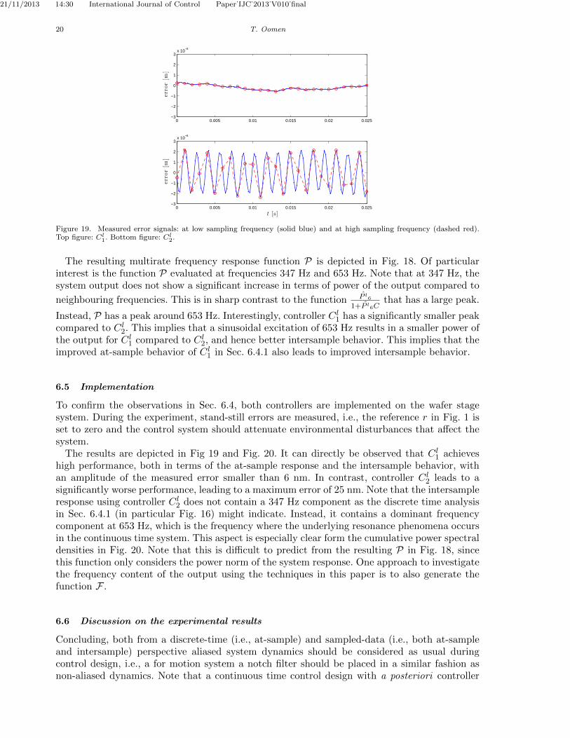
The results are depicted in Fig 19 and Fig. 20. It can directly be observed that C l1 achieveshigh performance, both in terms of the at-sample response and the intersample behavior, withan amplitude of the measured error smaller than 6 nm. In contrast, controller C l2 leads to asignificantly worse performance, leading to a maximum error of 25 nm. Note that the intersampleresponse using controller C l2 does not contain a 347 Hz component as the discrete time analysisin Sec. 6.4.1 (in particular Fig. 16) might indicate. Instead, it contains a dominant frequencycomponent at 653 Hz, which is the frequency where the underlying resonance phenomena occursin the continuous time system. This aspect is especially clear form the cumulative power spectraldensities in Fig. 20. Note that this is difficult to predict from the resulting P in Fig. 18, sincethis function only considers the power norm of the system response. One approach to investigatethe frequency content of the output using the techniques in this paper is to also generate thefunction F .

6.6 Discussion on the experimental results

Concluding, both from a discrete-time (i.e., at-sample) and sampled-data (i.e., both at-sampleand intersample) perspective aliased system dynamics should be considered as usual duringcontrol design, i.e., a for motion system a notch filter should be placed in a similar fashion asnon-aliased dynamics. Note that a continuous time control design with a posteriori controller



1 10 100 500 25000

0.5

1

1.5

2

2.5

3x 10

−16

f [Hz]

CPS(error)

1 10 100 500 25000

0.5

1

1.5

2

2.5

3x 10

−16

f [Hz]

Figure 20. Cumulative power spectral density of measured error signals: at low sampling frequency (solid blue) and at highsampling frequency (dashed red). Left figure: Cl

1 Right figure: Cl2.

discretisation is generally inferior to both sampled-data and discrete time control designs, asthese will not automatically attenuate the aliased resonance phenomenon. In other words, thesewill deliver poor performance that is similar to controller C l2.

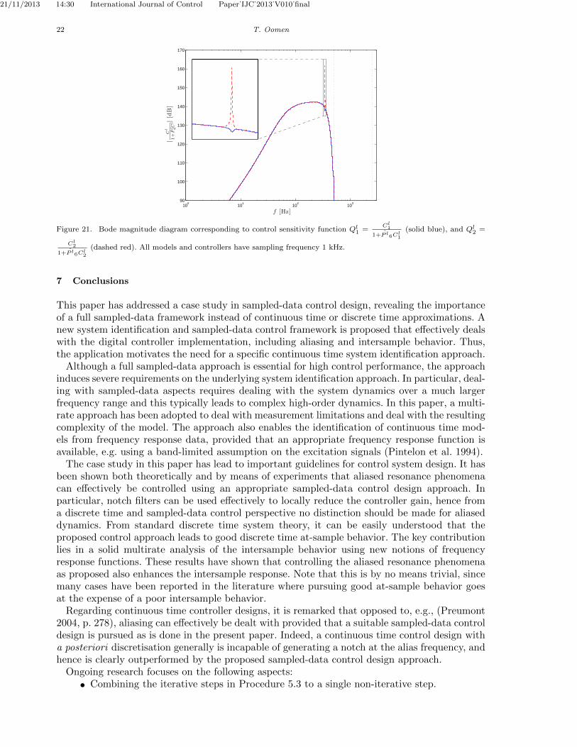
The enhanced performance of controller C l1 compared to C l2 can be understood by analyzing

(14). Indeed, note that Ql in the setup of Fig. 17 corresponds to Ql = Cl

1+P lCl . Hence Ql is the

only term that actually depends on C l in the computation of the multirate frequency responsefunctions in Definition 5.2. Clearly, due to the presence of the notch filter in C l1, Ql1 is smallerat 347 Hz, and since Gh11 = 0, this leads to a smaller intersample response compared to C l2.

Remark 3 : In certain situations, resonance phenomena in motion control are dealt with by‘inverting’ the notch filter, i.e., increasing the locally gain of the controller instead of decreasingit. This can only be done if the phase of the resulting loop-gain has positive real part, in which

case∣∣∣ 1

1+P lCl

∣∣∣ < 1 (see, e.g., Oomen et al. (2013, Fig. 16-17) for an example). However, from

the perspective of the results in this paper, such an approach should be followed with caution.Indeed, the above analysis regarding Ql reveals that this may potentially lead to poor intersamplebehavior, e.g., as in Oomen et al. (2007).

Remark 4 : The intersample analysis in Fig. 18 clearly reveals the poor intersample behaviorassociated with C l2. However, it is remarked that the actual results may be more severe thanpredicted by P due to the mismatch in Fig. 11. Hence, the accuracy of P may be improvedby enhancing the correspondence between the downsampled model and the identified frequencyresponse function and model at the low sampling frequency f l.

Remark 5 : The obtained results shed light on the required order of the models that areidentified in Sec. 6.3.1 and Sec. 6.3.2. Indeed, a 6th order model is obtained at the samplingfrequency f l, which accurately represents the aliased resonance phenomenon at 349 Hz. Thisresonance is essential for obtaining the notch in C l1, see Fig. 14. Indeed, otherwise the standardPID type controller C l2 would have been obtained. This immediately reveals the advantages ofthe proposed control design framework, since such a PID controller would lead to the disastrousperformance associated with C l2 in Fig. 19 (bottom). Note that the 60th order model only isused for intersample behavior analysis, and does not directly affect the order of the designedcontroller. Still, a lower order of the fast sampled model is preferable, provided that it can beidentified in a control-relevant manner. See also Sec. 6.3.1 and Sec. 7 for a further explanation.


22 T. Oomen

100

101

102

103

90

100

110

120

130

140

150

160

170

|C

l

1+P

l 6C

l|[dB]

f [Hz]

Figure 21. Bode magnitude diagram corresponding to control sensitivity function Ql1 =

Cl1

1+P l6Cl1

(solid blue), and Ql2 =

Cl2

1+P l6Cl2

(dashed red). All models and controllers have sampling frequency 1 kHz.

7 Conclusions

This paper has addressed a case study in sampled-data control design, revealing the importanceof a full sampled-data framework instead of continuous time or discrete time approximations. Anew system identification and sampled-data control framework is proposed that effectively dealswith the digital controller implementation, including aliasing and intersample behavior. Thus,the application motivates the need for a specific continuous time system identification approach.

Although a full sampled-data approach is essential for high control performance, the approachinduces severe requirements on the underlying system identification approach. In particular, deal-ing with sampled-data aspects requires dealing with the system dynamics over a much largerfrequency range and this typically leads to complex high-order dynamics. In this paper, a multi-rate approach has been adopted to deal with measurement limitations and deal with the resultingcomplexity of the model. The approach also enables the identification of continuous time mod-els from frequency response data, provided that an appropriate frequency response function isavailable, e.g. using a band-limited assumption on the excitation signals (Pintelon et al. 1994).

The case study in this paper has lead to important guidelines for control system design. It hasbeen shown both theoretically and by means of experiments that aliased resonance phenomenacan effectively be controlled using an appropriate sampled-data control design approach. Inparticular, notch filters can be used effectively to locally reduce the controller gain, hence froma discrete time and sampled-data control perspective no distinction should be made for aliaseddynamics. From standard discrete time system theory, it can be easily understood that theproposed control approach leads to good discrete time at-sample behavior. The key contributionlies in a solid multirate analysis of the intersample behavior using new notions of frequencyresponse functions. These results have shown that controlling the aliased resonance phenomenaas proposed also enhances the intersample response. Note that this is by no means trivial, sincemany cases have been reported in the literature where pursuing good at-sample behavior goesat the expense of a poor intersample behavior.

Regarding continuous time controller designs, it is remarked that opposed to, e.g., (Preumont2004, p. 278), aliasing can effectively be dealt with provided that a suitable sampled-data controldesign is pursued as is done in the present paper. Indeed, a continuous time control design witha posteriori discretisation generally is incapable of generating a notch at the alias frequency, andhence is clearly outperformed by the proposed sampled-data control design approach.

Ongoing research focuses on the following aspects:

• Combining the iterative steps in Procedure 5.3 to a single non-iterative step.


REFERENCES 23

• Refining the identification criterion (13) to address sampled-data control-relevant ob-jectives to extend the results of Oomen et al. (2013), Oomen and Bosgra (2012) to themultirate case, see Sec. 6.3.1 for a discussion on this aspect.

• Addressing the aspect of model quality (including variance) in the multirate frequencyresponse functions in Definition 5.2.

• Enhancing the continuous time model identification step and address the full continu-ous time intersample behavior in the presented framework. In particular, in this paper,discrepancies between fast sampled/continuous time models and their slow sampled dis-cretisation were found. The cause of these discrepancies has to be investigated and alter-native identification methods may be considered, see, e.g., Young (1998, Sec. 3), whereaccurate results for the vibration modes of a cantilever beam are obtained through analternative time domain continuous time identification approach. An additional impor-tant advantage associated with the use of continuous time models is that the model canbe discretised at different sampling frequencies. In particular, using the results presentedhere, this allows to choose the best sampling frequency in the case of aliased resonancephenomena.

• Experimental investigation of the model discrepancies in Sec. 6.3.2.

• Dealing with the complexity induced by the sampled-data problem formulation. In par-ticular, the increased sampling frequency reveals higher order dynamics. This leads toa numerically challenging identification problem. In particular, to obtain the high ordermodel in Sec. 6.3.1, the numerically reliable approach in Oomen and Steinbuch (2014),see also Bultheel et al. (2005), is adopted. Ongoing work focuses on extending theseresults to enhance efficiency, see Van Herpen et al. (2012).

Acknowledgement

The author would like to thank Marc van de Wal, Robbert van Herpen, and Maarten Steinbuchare for their contribution to this research, and the late Okko Bosgra is gratefully acknowledgedfor fruitful discussions in an early stage of this research. Finally, the author would like to thankthe reviewers and guest editors for their constructive comments that have improved this paper.Philips Innovation Services is gratefully acknowledged for access to the experimental setup andtheir support for this research. This work is partially supported by the Innovational ResearchIncentives Scheme under the VENI grant Precision Motion: Beyond the Nanometer (no. 13073)awarded by NWO (The Netherlands Organisation for Scientific Research) and STW (DutchScience Foundation).

References

Astrom, K.J., Hagander, P., and Sternby, J. (1984), “Zeros of Sampled Systems,” Automatica, 20, 31–38.

Astrom, K.J., and Wittenmark, B., Computed-Controlled Systems: Theory and Design, second ed., Englewood Cliffs, NJ,USA: Prentice-Hall (1990).

Bamieh, B., Pearson, J.B., Francis, B.A., and Tannenbaum, A. (1991), “A Lifting Technique for Linear Periodic SystemsWith Applications to Sampled-Data Control,” Syst. Contr. Lett., 17, 79–88.

B lachuta, M.J., and Grygiel, R.T. (2008), “Sampling of Noisy Signals: Spectral vs Anti-Aliasing Filters,” in IFAC 17thTriennial World Congress, Seoul, Korea, pp. 7576–7581.

B lachuta, M.J., and Grygiel, R.T. (2009), “Are Anti-Aliasing Filters Really Necessary for Sampled-Data Control?,” in Proc.2009 Americ. Contr. Conf., St. Louis, MO, USA, pp. 3200–3205.

Bultheel, A., van Barel, M., Rolain, Y., and Pintelon, R. (2005), “Numerically Robust Transfer Function Modeling FromNoisy Frequency Domain Data,” IEEE Trans. Automat. Contr., 50, 1835–1839.

de Callafon, R.A., de Roover, D., and Van den Hof, P.M.J. (1996), “Multivariable Least Squares Frequency Domain Iden-tification using Polynomial Matrix Descriptions,” in Proc. 35th Conf. Dec. Contr., Kobe, Japan, pp. 2030–2035.

de Callafon, R.A., and Van den Hof, P.M.J. (2001), “Multivariable Feedback Relevant System Identification of a WaferStepper System,” IEEE Trans. Contr. Syst. Techn., 9, 381–390.

Cantoni, M.W., and Glover, K. (1997), “Frequency-Domain Analysis of Linear Periodic Operators With Application toSampled-Data Control Design,” in Proc. 1997 Conf. Dec. Contr., San Diego, CA, USA, pp. 4318–4323.

Chen, T., and Francis, B., Optimal Sampled-Data Control Systems, London, UK: Springer (1995).


24 REFERENCES

Delgado, R.A., Aguero, J.C., Goodwin, G.C., and Yuz, J.I. (2011), “Two-Degree-of-Freedom Anti-Aliasing Technique forWide-Band Networked Control,” in IFAC 18th Triennial World Congress, Milano, Italy, pp. 8884–8889.

Dullerud, G.E., Control of Uncertain Sampled-Data Systems, Boston, MA, USA: Birkhauser (1996).Freudenberg, J.S., Middleton, R.H., and Braslavsky, J.H. (1995), “Inherent Design Limitations for Linear Sampled-Data

Feedback Systems,” Int. J. Contr., 61, 1387–1421.Garnier, H., and Wang, L. (eds.) Identification of Continuous-Time Models from Sampled Data, Advances in Industrial

Control, London, UK: Springer-Verlag (2008).Gevers, M. (1993), “Towards a Joint Design of Identification and Control ?,” in Essays on Control : Perspectives in the

Theory and its Applications eds. H.L. Trentelman and J.C. Willems, Boston, MA, USA: Birkhauser, chap. 5, pp. 111–151.Goodwin, G.C., Aguero, J.C., Cea Garrido, M.E., Salgado, M.E., and Yuz, J.I. (2013), “Sampling and Sampled-Data

Models,” IEEE Contr. Syst. Mag., 33, 34–53.Goodwin, G.C., and Salgado, M. (1994), “Frequency Domain Sensitivity Functions for Continuous Time Systems Under

Sampled Data Control,” Automatica, 30, 1263–1270.Hara, S., Tetsuka, M., and Kondo, R. (1990), “Ripple Attenuation in Digital Repetitive Control Systems,” in Proc. 29th

Conf. Dec. Contr., Honolulu, HI, USA, pp. 1679–1684.Heath, W.P. (2001), “Bias of Indirect Non-Parametric Transfer Function Estimates for Plants in Closed Loop,” Automatica,

37, 1529–1540.van Herpen, R., Oomen, T., and Bosgra, O. (2012), “Bi-Orthonormal Basis Functions for Improved Frequency Domain

System Identification,” in Proc. 51st Conf. Dec. Contr., Maui, HI, USA, pp. 3451–3456.Hughes, P.C. (1987), “Space Structure Vibration Modes: How Many Exist? Which Ones Are Important?,” IEEE Contr.

Syst. Mag., 7, 22–28.LeVoci, P.A., and Longman, R.W. (2004), “Intersample Error in Discrete Time Learning and Repetitive Control,” in Proc.

AIAA/AAS Astrodynamics Specialist Conf. and Exhibit, Providence, RI, USA, pp. 1–24.Lindgarde, O., and Lennartson, B. (1997), “Performance and Robust Frequency Response for Multirate Sampled-Data

Systems,” in Proc. 1997 Americ. Contr. Conf., Albuquerque, NM, USA, pp. 3877–3881.Ljung, L., System Identification: Theory for the User, second ed., Upper Saddle River, NJ, USA: Prentice Hall (1999).Oomen, T., and Bosgra, O. (2012), “System Identification for Achieving Robust Performance,” Automatica, 48, 1975–1987.Oomen, T., and Steinbuch, M. (To appear, 2014), “Identification for robust control of complex systems: Algorithm and

motion application,” Control-oriented modelling and identification: theory and applications, IET.Oomen, T., van de Wal, M., and Bosgra, O. (2007), “Design Framework for High-Performance Optimal Sampled-Data

Control With Application to a Wafer Stage,” Int. J. Contr., 80, 919–934.Oomen, T., van de Wijdeven, J., and Bosgra, O. (2009), “Suppressing Intersample Behavior in Iterative Learning Control,”

Automatica, 45, 981–988.Oomen, T., van de Wijdeven, J., and Bosgra, O. (2011), “System identification and low-order optimal control of intersample

behavior in ILC,” IEEE Trans. Automat. Contr., 56, 2734–2739.Oomen, T., van Herpen, R., Quist, S., van de Wal, M., Bosgra, O., and Steinbuch, M. (2013), “Connecting System Identi-

fication and Robust Control for Next-Generation Motion Control of a Wafer Stage,” To appear in IEEE Trans. Contr.Syst. Techn..

Pintelon, R., Guillaume, P., Rolain, Y., Schoukens, J., and Van hamme, H. (1994), “Parametric Identification of TransferFunctions in the Frequency Domain - A Survey,” IEEE Trans. Automat. Contr., 39, 2245–2260.

Pintelon, R., Schoukens, J., McKelvey, T., and Rolain, Y. (1996), “Minimum Variance Bounds for OverparameterizedModels,” IEEE Trans. Automat. Contr., 41, 719–720.

Pintelon, R., Schoukens, J., and Rolain, Y. (2000), “Box-Jenkins Continuous-Time Modeling,” Automatica, 36, 983–991.Pintelon, R., and Schoukens, J. (1997), “Identification of Continuous-Time Systems Using Arbitrary Signals,” Automatica,

33, 991–994.Pintelon, R., and Schoukens, J. (2001), “Measurement of Frequency Response Functions Using Periodic Excitations, Cor-

rupted by Correlated Input/Output Errors,” IEEE Trans. Inst. Meas., 50, 1753–1760.Pintelon, R., and Schoukens, J., System Identification: A Frequency Domain Approach, second ed., New York, NY, USA:

IEEE Press (2012).Preumont, A., Vibration Control of Active Structures: An Introduction, second ed., Vol. 96 of Solid Mechanics and Its

Applications, New York, NY, USA: Kluwer Academic Publishers (2004).Quinn, W.J., and Williamson, S.E. (1985), “A Frequency Response Method for Predicting the Level of Intersample Activity

in Discrete Systems,” Int. J. Contr., 41, 429–444.Rao, G.P., and Unbehauen, H. (2006), “Identification of Continuous-Time Systems,” IEE Proc.-Control Theory Appl., 153,

185–220.Riggs, D.J., and Bitmead, R.R. (2013), “Rejection of Aliased Disturbances in a Production Pulsed Light Source,” IEEE

Trans. Contr. Syst. Techn., 21, 480–488.Rijlaarsdam, D., Oomen, T., Nuij, P., Schoukens, J., and Steinbuch, M. (2012), “Uniquely Connecting Frequency Domain

Representations for Given Order Polynomial Wiener-Hammerstein Systems,” Automatica, 48, 2381–2384.Schonhoff, U., and Nordmann, R. (2002), “A H∞-Weighting Scheme for PID-like Motion Control,” in Proc. 2002 Conf.

Contr. Appl., Glasgow, Scotland, pp. 192–197.Schrama, R.J.P. (1992), “Accurate Identification for Control: The Necessity of an Iterative Scheme,” IEEE Trans. Automat.

Contr., 37, 991–994.Skogestad, S., and Postlethwaite, I., Multivariable Feedback Control: Analysis and Design, second ed., West Sussex, UK:

John Wiley & Sons (2005).Smith, R.S. (1998), “Closed-Loop Identification of Flexible Structures: An Experimental Example,” J. Guid., Contr., Dyn.,

21, 435–440.de Souza, C.E., and Goodwin, G.C. (1984), “Intersample Variances in Discrete Minimum Variance Control,” IEEE Trans.

Automat. Contr., 29, 759–761.Steinbuch, M., and Norg, M.L. (1998), “Advanced Motion Control: An Industrial Perspective,” Eur. J. Contr., 4, 278–293.Van den Hof, P.M.J., and Schrama, R.J.P. (1995), “Identification and Control - Closed-loop Issues,” Automatica, 31, 1751–

1770.van de Wal, M., van Baars, G., Sperling, F., and Bosgra, O. (2002), “Multivariable H∞/µ Feedback Control Design for

High-Precision Wafer Stage Motion,” Contr. Eng. Prac., 10, 739–755.Weller, S.R., Moran, W., Ninness, B., and Pollington, A.D. (2001), “Sampling Zeros and the Euler-Frobenius Polynomials,”


REFERENCES 25

IEEE Trans. Automat. Contr., 46, 340–343.Yamamoto, Y. (1994), “A Function Space Approach to Sampled Data Control Systems and Tracking Problems,” IEEE

Trans. Automat. Contr., 39, 703–713.Yamamoto, Y., and Khargonekar, P.P. (1996), “Frequency Response of Sampled-Data Systems,” IEEE Trans. Automat.

Contr., 41, 166–176.Young, P. (1998), “Data-Based Mechanistic Modeling of Engineering Systems,” J. Vibr. Contr., 4, 5–28.

Documents

RESEARCH ARTICLE Controlling Aliased Dynamics in … · RESEARCH ARTICLE Controlling Aliased Dynamics in Motion Systems? ... Garnier and Wang 2008, Pintelon and Schoukens 1997)