Research Article Feature-based cartographic modelling

Research Article

Feature-based cartographic modelling

KEITH FRENCH and XINGONG LI*

Department of Geography, University of Kansas, Lawrence, KS 66045, USA

(Received 19 September 2007; in final form 13 September 2008 )

Cartographic modelling operations provide powerful tools for analysing and

manipulating geographic data in the raster data model. This research extends

these operations to the vector data model. It first discusses how the spatial scopes

of analysis can be defined for point, line, and polygon features analogous to the

raster cell. Then it introduces the local, focal, and zonal operations available for

vector features, followed by providing a prototype syntax that might guide the

implementation of these operations. Through example applications, this research

also demonstrates the usefulness of these operations by comparing them with

traditional vector spatial analysis.

Keywords: Map algebra; Vector data model; Spatial analysis

1. Introduction

Cartographic modelling (also called map algebra) operations provide powerful tools

for analysing and manipulating geographic data in the raster data model. The

operations are grouped into local, focal, and zonal classes based on the spatial scope

of the operations (Tomlin 1990). The principle analysis units are raster cells. Local

operations are those that calculate cell values on the output raster layer using cell

values on the input raster layers at the same location. Focal operations are those

that calculate output cell values using the input cell values within their respective

neighbourhoods. A neighbourhood is a set of cells that bear certain relationships to

the neighbourhood focus. Zonal operations calculate output cell values using the

input cell values within the same zones. A zone is a set of cells representing a two-

dimensional (2D) area.

The cartographic modelling operations have been expanded upon since their

inception. Chan and White (1987) implemented the operations using an object-

oriented programming language. Scott (1999) extended the original 2D cartographic

modelling operations into three dimensional raster datasets (i.e. voxels). A similar

extension was also made for spatio-temporal datasets where the third dimension is

time (Mennis et al. 2005). Cartographic modelling operations for vector fields where

cell values are vectors rather than scalar measurements were also developed

(Hodgson and Gaile 1999, Li and Hodgson 2004, Wang and Pullar 2005). Caldwell

(2000) added new operations (called flag operations) that mark the locations within

neighbourhoods and zones where a condition is met. Haklay’s map calculus (2004)

allowed for operations between layers represented by piecewise or global

mathematical functions. Although these are important advancements, the original

Inte

rnati

on

al

Jo

urn

al

of

Geo

gra

ph

ical

Info

rmati

on

Scie

nce

gis

170324.3

d4/1

1/0

819:1

3:1

2T

he

Charlesw

ort

hG

roup,

Wakefield

+44(0

)1924

369598

-R

ev

7.5

1n/W

(Jan

20

2003)

349414

*Corresponding author. Email: [email protected]

International Journal of Geographical Information Science

Vol. 000, No. 000, 0 Month 2008, 1–24

0

5

10

15

20

25

30

35

40

45

0

5

10

15

20

25

30

35

40

45

International Journal of Geographical Information ScienceISSN 1365-8816 print/ISSN 1362-3087 online # 2008 Taylor & Francis

http://www.tandf.co.uk/journalsDOI: 10.1080/13658810802492462

cartographic modelling framework and aforementioned extensions are all exclusive

to the raster data model.

Although converting vector data to raster data to use cartographic modelling

operations is always a possibility, loss of precise location or loss of entire features

can occur if the chosen cell size is not carefully considered. Furthermore, reducing

cell size to accommodate small features can generate excessively large datasets.

Realising that polygons in the vector data model can be manipulated in a way that

resembles raster cells, Tobler (1995) suggested some focal operations on polygons

(called resels) that have irregular polygon neighbours. Along the same line, Ledoux

and Gold (2006) discussed map algebra operations on Voronoi diagrams that

represent fields with irregular polygon tessellations. While the polygons can be

treated much like raster cells, performing cartographic modelling operations on

points and lines has not been systematically studied.

This research extends the cartographic modelling operations to the vector data

model. The next section discusses the spatial scopes for point, line, and polygon

features and how features are selected and adjusted. Section 3 introduces local,

focal, and zonal operations for different vector data types. Section 4 ties the

operations into an operational syntax and discusses some implementation issues.

Several application examples are provided in section 5 to demonstrate that the

proposed framework is valuable to spatial analysis in the vector data model. Section

6 compares the vector cartographic modelling framework to the original raster

framework. The last section draws some conclusions.

2. Vector cartographic modelling

Cartographic modelling in the vector data model (hereinafter referred to as VCM) is

complicated by the fact that vector data lacks the uniformity of the raster grid. In

the raster data model, once the output cell size is determined, the spatial scopes of

the operations are defined based on this uniform and atomic spatial granule. Local

in the raster cartographic modelling framework refers to a single cell, focal refers to

the cells within the neighbourhood of a focus cell, and zonal is a set of cells with the

same value. In the vector data model, however, there is not such a uniform spatial

granule. This requires us to define what exactly local, focal, and zonal are in the

context of discrete points, lines, and polygons.

It should be noted that geographic features (hereinafter simply called features) on

a vector layer can have multiple attributes, unlike the cells on a raster layer, which

hold only a single value. Therefore, the desired attribute to be used in a vector

cartographic modelling operation must be explicitly indicated. In addition, features

have geometric properties that may vary from feature to feature. Finally, unlike

raster cells which have uniform spatial relationships with nearby cells, vector

features may have specific spatial relationships with nearby features which are not

necessarily uniform from feature to feature. These differences open up new analysis

possibilities. First, we will take a look at how each of the three classes of raster

cartographic modelling operations can be defined with respect to each of the three

feature types in the vector data model.

2.1 Local scope

In the raster data model, since the smallest spatial unit is the cell, a local scope refers

to individual cells. In the vector data model, the smallest spatial unit—for all

Inte

rnati

on

al

Jo

urn

al

of

Geo

gra

ph

ical

Info

rmati

on

Scie

nce

gis

170324.3

d4/1

1/0

819:1

3:1

3T

he

Charlesw

ort

hG

roup,

Wakefield

+44(0

)1924

369598

-R

ev

7.5

1n/W

(Jan

20

2003)

349414

2 K. French and X.G. Li

0

5

10

15

20

25

30

35

40

45

0

5

10

15

20

25

30

35

40

45

practical purposes—is the feature. We propose two types of vector layers in a local

operation, the focus layer and the value layer. The focus layer defines the local scope

of the operation. Each feature on the focus layer defines a local spatial scope of

operation. The value layer stores the features to which the features on the focus layer

will be spatially compared. There may be multiple value layers for local operations.

The chosen operations are carried out only on those features on the value layer(s)

that are in the local scope of each feature on the focus layer. The result of a local

operation is a new vector layer that is spatially identical to the focus layer, but with

each feature having a new attribute that stores the result from the selected operation.

In practise, the new attribute may simply be added to the existing features in the

focus layer rather than creating a new vector layer. There are three types of focus

layers for local operations, one for each of the three vector data types. They are

discussed in turn, as each is handled differently.

Points are zero dimensional features and they are unique when considering

locality. A point is local to itself and any other point that is at exactly the same

location is also local to the point. A line is local to a point only if the line crosses

exactly over the point. A polygon that encompasses a point or whose border crosses

over the point is local to the point. Locality with respect to points is not generally

useful because for two points to be local to each other they must lie in exactly the

same location. Typically, this only occurs when the points are, in fact, representing

the same real-world object. One might thus argue that a small tolerance could be

used to specify point locality. This, however, can be accommodated through a

neighbourhood definition with a focal operation. Locality with respect to points for

local operations is binary in nature; either a feature on the value layer intersects a

focus point or it does not. This can change with the other data types as we will see

next.

Lines have one dimension and any point that falls directly on a focus line is local

to the focus line. A line is local to itself, and any other lines that have the same

location and geometry are also local to the line. A polygon that intersects a focus

line is local to the focus line as well. In the last two examples, it is possible that a

partial locality exists, that is to say, only a portion of the value feature intersects the

focus feature. When this is the case, the features remain local to the focus feature,

but have gone beyond binary. This is discussed in more detail in section 2.4.

Polygons as focus features are arguably the most useful in terms of determining

locality. This is because it is the only geometry type that can fully contain all other

geometric types. Any point inside a polygon or on its border is local to the polygon.

Any line or polygon intersecting it is also local, but may again be subject to partial

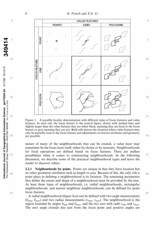
locality. A polygon is, like the point and line, local to itself. Figure 1 illustrates a

possible locality determination with different types of focus and value features. Bold

cells denote the situations where partial locality may occur. Partial locality can be

dealt with in a number of ways as discussed in section 2.4.

2.2 Focal scope

Focal operations are performed within the spatial scope known as neighbourhoods.

In the raster data model, the spatial extent of a neighbourhood is a function of cell

size and neighbourhood type and size, and is defined as a set of cells. The vector

data model introduces several new ways of defining neighbourhoods based on the

topology among focus features. Much like local operations, focal operations have a

focus layer and a value layer or layers. It is important to note that because of the

Inte

rnati

on

al

Jo

urn

al

of

Geo

gra

ph

ical

Info

rmati

on

Scie

nce

gis

170324.3

d4/1

1/0

819:1

3:1

3T

he

Charlesw

ort

hG

roup,

Wakefield

+44(0

)1924

369598

-R

ev

7.5

1n/W

(Jan

20

2003)

349414

Feature-based cartographic modelling 3

0

5

10

15

20

25

30

35

40

45

0

5

10

15

20

25

30

35

40

45

nature of many of the neighbourhoods that can be created, a value layer may

sometimes be the focus layer itself, either by choice or by necessity. Neighbourhoods

for focal operations are defined based on focus features. There are endless

possibilities when it comes to constructing neighbourhoods. In the following

discussion, we describe some of the practical neighbourhood types and leave the

reader to discover others.

2.2.1 Neighbourhoods for points. Points are unique in that they have location but

no other geometric attributes such as length or area. Because of this, the only role a

point plays in defining a neighbourhood is its location. The remaining parameters

that define the extent and shape of a neighbourhood must be provided by the user.

At least three types of neighbourhoods, i.e. radial neighbourhoods, rectangular

neighbourhoods, and nearest neighbour neighbourhoods, can be defined for point

focus features.

A radial neighbourhood (figure 2(a)) can be defined with two angle measurements

(hmin, hmax) and two radius measurements (rmin, rmax). The neighbourhood is the

region bounded by angles hmin and hmax, and the two arcs with radii rmin and rmax.

The zero angle extends due east from the focus point and positive angles are

Inte

rnati

on

al

Jo

urn

al

of

Geo

gra

ph

ical

Info

rmati

on

Scie

nce

gis

170324.3

d4/1

1/0

819:1

3:1

3T

he

Charlesw

ort

hG

roup,

Wakefield

+44(0

)1924

369598

-R

ev

7.5

1n/W

(Jan

20

2003)

349414

Figure 1. A possible locality determination with different types of focus features and valuefeatures. In each cell, the focus feature is the central figure, drawn with dashed lines andslightly larger than the value features that are either black, meaning they are local to the focusfeature or gray meaning they are not. Bold cells denote the situation where value features mayonly be partially local to the focus feature and adjustments on feature attributes and geometryare possible.


0

5

10

15

20

25

30

35

40

45

0

5

10

15

20

25

30

35

40

45

measured counterclockwise from the zero angle while negative angles are measured

clockwise. Note that this follows the standard mathematic convention for radial

measurements. If no angle measurements and only one radial measurement are

specified, the neighbourhood will be a simple circular buffer around the focus point,

with rmax as the radius. If no angle measurements and two radial measurements are

specified, the neighbourhood will be an annulus, with an inner radius of rmin and an

outer radius of rmax. If rmin is omitted and two angles are given, a wedge

neighbourhood is defined by the two radials and a single arc with radius rmax.

Rectangular neighbourhoods (figure 2(b)) for focus points can also be defined

with four parameters, height (H), width (W), pivot point, and rotation angle (h). The

pivot point is the rectangle’s initial location with respect to the focus point before

applying any rotation to the rectangle. The pivot point can be located anywhere, but

for practical purposes we only consider three locations (figure 2(c)): upper left

corner, top edge centre, and centroid of the rectangle. A rectangle measured from

Inte

rnati

on

al

Jo

urn

al

of

Geo

gra

ph

ical

Info

rmati

on

Scie

nce

gis

170324.3

d4/1

1/0

819:1

3:1

9T

he

Charlesw

ort

hG

roup,

Wakefield

+44(0

)1924

369598

-R

ev

7.5

1n/W

(Jan

20

2003)

349414

Figure 2. Neighbourhoods for focus points: (a) a radial neighbourhood; (b) a rectangularneighbourhood; (c) different pivot points for a rectangular neighbourhood with rotationangles of 0, 30, and 45 degrees; (d) a nearest-neighbour neighbourhood; (e) a distanceneighbourhood; (f) proximal region neighbourhoods.


0

5

10

15

20

25

30

35

40

45

0

5

10

15

20

25

30

35

40

45

the upper left corner will have a width (W) that stretches due east of the pivot point,

and a height (H), that stretches due south. The rotation angle (h) is then applied to

the rectangle at the pivot point. The rotation angle is measured from the same zero

angle line used in radial neighbourhoods to the line that has been given the width

measurement. The rectangle is rotated either counterclockwise with positive angles

or clockwise with negative angles. While only rectangle neighbourhoods are

discussed here, the same neighbourhoods could easily be extended to shapes such as

triangles or hexagons.

Both radial neighbourhoods and rectangular neighbourhoods can be offset from

focus points. An offset can be defined by the offsets in the X and Y dimension (i.e.

DX and DY) or by an angle and distance value. This will allow for a shift of the

neighbourhood in relation to the focus point.

Neighbourhoods can also be defined for focus points in several other ways. First,

neighbourhoods can be defined based on the order of nearness to a focus point by

including a certain number of nearest points (figure 2(d)). Second, neighbourhoods

can be defined by the points that are within a certain distance from focus points

(figure 2(e)). Finally, the proximal regions (also called Thiessen polygons or Voronoi

diagrams) of focus points can also be used as their respective neighbourhoods

(figure 2(f)). As seen in figure 2(f), one distinctive feature of proximal neighbour-

hoods is that they cover the entire extent of the data layer without gaps and overlaps

between any neighbourhoods.

2.2.2 Neighbourhoods for lines. Lines differ from points in two important ways.

First, they have length and they are unbroken over this length. Whereas two points

can only overlap completely, or not overlap at all, lines can overlap completely,

partially, at one or several points, or not at all. Secondly, lines may connect to each

other to form networks and thus provide the basis to form neighbourhoods based

on line connectivity. Buffer neighbourhoods (figure 3(a)) from focus lines can be

defined by two distance measurements (bmin, bmax). If bmin is omitted the

neighbourhood consists of the region in which the shortest distance to the focus

line is least than or equal to bmax.

A neighbourhood can also be formed based on the connectivity between the focus

line and its neighbour lines. A zero-order connectivity neighbourhood will be the

focus line itself. A first-order connectivity neighbourhood includes all lines that

connect to the focus line, and the focus line itself if an accumulative neighbourhood

is desired. A second-order connectivity neighbourhood would include all those lines

that connect to the lines in the first-order connectivity neighbourhood. Figure 3(b)

shows an example second-order connectivity neighbourhood where the neighbour-

hood lines are in bold. Note that this example is an accumulative connectivity

neighbourhood in that it includes the first-order and zero-order neighbourhoods. In

addition to connectivity, neighbourhoods can also be defined based on the distance

in the network from focus lines. In this case the neighbourhood would consist of all

the lines and partial lines connected to a focus line up to a certain distance as

measured from the ends of the focus line (figure 3(c)). Finally, as with points, the

proximal regions of lines can be used as their respective neighbourhoods

(figure 3(d)).

2.2.3 Neighbourhoods for polygons. Buffer neighbourhoods (figure 4(a)) for focus

polygons can be defined by two distance measurements (bmin, bmax), and the

resultant neighbourhood will be the region formed by those measurements from the

Inte

rnati

on

al

Jo

urn

al

of

Geo

gra

ph

ical

Info

rmati

on

Scie

nce

gis

170324.3

d4/1

1/0

819:1

3:2

9T

he

Charlesw

ort

hG

roup,

Wakefield

+44(0

)1924

369598

-R

ev

7.5

1n/W

(Jan

20

2003)

349414


0

5

10

15

20

25

30

35

40

45

0

5

10

15

20

25

30

35

40

45

edges of the polygon. The neighbourhood of polygons adjacent to a focus polygon is

made in a similar fashion to the neighbourhoods made of lines based on line

connectivity. A zero-order adjacency neighbourhood will be the focus polygon itself.

A first-order adjacency neighbourhood includes all polygons that are immediately

adjacent to the focus polygon. A second-order adjacency neighbourhood includes all

those polygons that are adjacent to the first-order adjacency polygons. As with the

line connectivity neighbourhoods, these neighbourhoods can be inclusive or

exclusive. Figure 4(b) shows an example of exclusive second-order adjacency

neighbourhood. When gaps exist among focus polygons, the proximal regions of

the polygons could also be used as neighbourhoods (figure 4(c)).

The many kinds of neighbourhoods cannot be enumerated. Most of the

neighbourhoods given above are based on geometry and distance relationships to

the focus feature. However, neighbourhoods could also be defined based on some

Inte

rnati

on

al

Jo

urn

al

of

Geo

gra

ph

ical

Info

rmati

on

Scie

nce

gis

170324.3

d4/1

1/0

819:1

3:2

9T

he

Charlesw

ort

hG

roup,

Wakefield

+44(0

)1924

369598

-R

ev

7.5

1n/W

(Jan

20

2003)

349414

Figure 3. Neighbourhoods for focus lines: (a) a buffer neighbourhood defined by twodistance parameters; (b) a second order connectivity neighbourhood in bold lines; (c)neighbourhood (in bold lines) defined by the network distance to the focus line; (d)neighbourhoods defined by the proximal regions of focus lines.

Figure 4. Neighbourhoods for focus polygons: (a) buffer neighbourhood defined by twodistance parameters; (b) a second order adjacency neighbourhood in shaded polygons; (c)neighbourhoods defined by the proximal regions of focus polygons.


0

5

10

15

20

25

30

35

40

45

0

5

10

15

20

25

30

35

40

45

functional relationships to focus features for a specific application. For example, the

counties which are connected to a focus county by highways can serve as the

neighbourhood of the focus county. Those functional neighbourhoods can be

defined by using a table where each focus feature is associated to its neighbourhood

feature(s).

2.3 Zonal scope

A zone is a collection of features on the focus layer that have the same value for a

given attribute. For all practical purposes, the attribute is usually at nominal or

ordinal level. Interval and ratio attributes can be degraded into nominal or ordinal

values through several classification methods. These methods are a part of attribute

manipulation functions usually available in most database systems. If the features

comprising a zone are made available as a single feature (usually referred to as a

multi-part feature), then zonal operations become local operations. Likewise, when

each focus feature is a separate zone, a zonal operation is actually a local operation.

For all practical purposes, most zones consist of a set of polygons. However,

zones can also be made of a set of lines or points. These types of zones might be

practical when counting the value features that intersect the lines or points. All the

features in the same zone will have the same output value from a zonal operation.

To reduce redundancy, it may be useful to have a table that stores zone identifiers

and the output values from a zonal operation. This table can be joined back to the

focus layer with the zone identifiers.

2.4 Feature selection and geometry and attribute adjustment

Locality, neighbourhoods, and zones discussed above define the spatial scope of a

focus feature for local, focal, and zonal operations. A set of features on the value

layer is selected that intersects the focus feature’s spatial scope. It is with this set of

value features that cartographic modelling operations are carried out. However,

because of the lack of a uniform spatial granule such as the cells in the raster data

model, the value features and their attributes associated with a focus feature may

not be clearly defined, especially when a value feature only partially intersects a local

feature, neighbourhood, or zone. In many cases, the geometries or attributes of the

value features need to be adjusted based on intersection geometries. Here we identify

four types of feature selection/adjustment depending on how value features are

selected and how their geometries and attributes are adjusted.

First, value features are selected based on a certain topological relationship

between the value features and a local feature, neighbourhood, or zone. The original

geometries and attributes of the selected value features are used in calculations.

Topological relationships can be defined based on the dimensionally extended 9-

intersection model (DE9IM) developed by Egenhofer and Herring (1991) and

Clementini et al. (1993). For example, the ‘within’ relationship, which selects the

value features that fall inside a local feature, neighbourhood, and zone, can be

defined based on the intersections between interior, boundary, and exterior as

shown in table 1. With this relationship, any value feature that intersects any space

outside a local feature, neighbourhood, or zone is ignored. It is worth noting that

some topological relationships may only exist for certain combinations of geometric

types. For example, the ‘within’ relationship only exists for the combinations of

geometric types which are indicated as ‘Y’ in table 2. This type of selection, without

Inte

rnati

on

al

Jo

urn

al

of

Geo

gra

ph

ical

Info

rmati

on

Scie

nce

gis

170324.3

d4/1

1/0

819:1

3:3

7T

he

Charlesw

ort

hG

roup,

Wakefield

+44(0

)1924

369598

-R

ev

7.5

1n/W

(Jan

20

2003)

349414


0

5

10

15

20

25

30

35

40

45

0

5

10

15

20

25

30

35

40

45

any adjustment, can be specified by a text string which defines the topological

relationships used to select value features.

In the second case, all the value features that intersect with a local feature,

neighbourhood, and zone are selected. However, those value features that lie

partially inside a local feature, neighbourhood, or zone have their new geometries as

the portions that are within the local feature, neighbourhood, or zone. Adjustment

is made only on the geometries of the value features. The attributes of the value

features remain the same as their original values. Note that this is only a temporary

adjustment for the sake of the current operation and the input dataset is not altered.

It allows for the geometry of value features to be ‘clipped’, so that only the portions

of the value features lying inside the local feature, neighbourhood, or zone are

considered in an operation. This type of selection and adjustment is hereinafter

referred as the ON_GEOMETRY enumeration. The topological relationship and

the possible combinations of the geometric types for this enumeration are shown in

tables 3 and 4 respectively.

Similar to the second case, the geometry of value features are clipped into the

local feature, neighbourhood, and zone. However, adjustment is also made on the

attributes of the selected value features and is based on the intersection geometries

between value features and local features, neighbourhoods or zones. This can be

done in one of two ways. The intersection geometries can be compared with the

either the geometries of value features or that of local features, neighbourhoods, and

zones. It is important to note that intersection types must be the same in order to

make these comparisons. For example, if the intersection of two polygons results in

a line, the intersection line has to be compared with the boundaries, not area, of the

polygons. This type of adjustment is arguably the most useful, and as such we will

describe the two approaches in more detail.

In the first approach, intersection geometries are compared with value features,

and the geometric ratios, i.e. the ratios of length or area between the intersection

geometries and the value features are calculated. The first two rows of figure 5

demonstrate this type of adjustment. The ratios are then used to calculate new

Inte

rnati

on

al

Jo

urn

al

of

Geo

gra

ph

ical

Info

rmati

on

Scie

nce

gis

170324.3

d4/1

1/0

819:1

3:3

7T

he

Charlesw

ort

hG

roup,

Wakefield

+44(0

)1924

369598

-R

ev

7.5

1n/W

(Jan

20

2003)

349414

Table 1. The ‘within’ relationship defined based on the DE9IM. A ‘T’ in the table indicatesan intersection must exist while a ‘F’ means an intersection must not exist. A ‘*’ representsthat it does not matter if an intersection exists or not. This relationship can be specified as a

string of ‘T*F**F***’.

Local feature, neighbourhood, or zone

Value feature Interior Boundary ExteriorInterior T * FBoundary * * FExterior * * *

Table 2. Possible combinations of geometric types with the ‘within’ relationship. A ‘Y’ in thetable indicates the combination is possible while an ‘N’ means the combination is impossible.


Value feature Point Line PolygonPoint Y Y YLine N Y YPolygon N N Y


0

5

10

15

20

25

30

35

40

45

0

5

10

15

20

25

30

35

40

45

attribute values for the value features before operations are performed. This type of

selection and adjustment is hereinafter referred to as OVER_VALUE_FEATURE.

The topological relationship and the possible combinations of geometric types for

this enumeration are shown in tables 5 and 6 respectively.

In the second approach, intersection geometries are compared with local features,

neighbourhoods, or zones and the ratios between intersection geometries and local

features, neighbourhoods, or zones are used to adjust the attributes of the value

features, as shown in the last two rows of figure 5. This type of adjustment is only

possible if the intersection geometry is the same type as the local, neighbourhood, or

zone geometry. There may be situations where local features, neighbourhoods, or

zones are not completely covered by value features. In this case, the ratio can be

calculated based on either the entire length or area of the local features,

neighbourhoods, and zones or just the portions of the length or area of the local

feature, neighbourhood, or zone that is covered by value features. This type of

selection and adjustment is hereinafter referred as OVER_LNZ. The topological

relationship and the possible combinations of geometric types for this enumeration

are shown in tables 7 and 8 respectively.

The OVER_VALUE_FEATURE adjustment is appropriate when an attribute

represents a summary within a value feature. An example of such an attribute is the

population attribute associated with a census polygon. The population that falls into

a local feature, neighbourhood, or zone should be calculated using this adjustment.

Conversely, when the attribute applies over the entire value feature, such as land use

types or precipitation rate, the attribute does not need to be adjusted. Both the

OVER_VALUE_FEATURE and OVER_LNZ enumeration adjust the attributes of

selected value features solely based on the geometric proportion of length and area.

Inte

rnati

on

al

Jo

urn

al

of

Geo

gra

ph

ical

Info

rmati

on

Scie

nce

gis

170324.3

d4/1

1/0

819:1

3:3

8T

he

Charlesw

ort

hG

roup,

Wakefield

+44(0

)1924

369598

-R

ev

7.5

1n/W

(Jan

20

2003)

349414

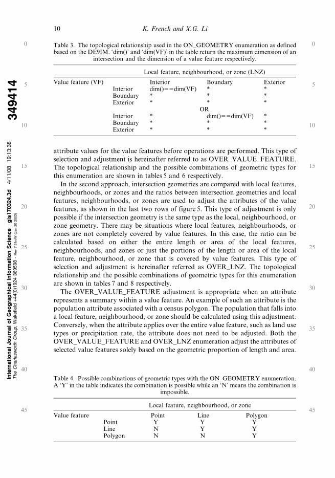
Table 3. The topological relationship used in the ON_GEOMETRY enumeration as definedbased on the DE9IM. ‘dim()’ and ‘dim(VF)’ in the table return the maximum dimension of an

intersection and the dimension of a value feature respectively.

Local feature, neighbourhood, or zone (LNZ)

Value feature (VF) Interior Boundary ExteriorInterior dim()55dim(VF) * *Boundary * * *Exterior * * *

ORInterior * dim()55dim(VF) *Boundary * * *Exterior * * *

Table 4. Possible combinations of geometric types with the ON_GEOMETRY enumeration.A ‘Y’ in the table indicates the combination is possible while an ‘N’ means the combination is

impossible.


Value feature Point Line PolygonPoint Y Y YLine N Y YPolygon N N Y


0

5

10

15

20

25

30

35

40

45

0

5

10

15

20

25

30

35

40

45

Although those approaches are simple they do not require any ancillary data that

are usually necessary in most advanced methods (Mennis and Hultgren 2006).

3. Operations

The operations that are performed on the value features depend on what properties

of the value features are used. Table 9 lists some of the most common operations, the

properties of the value feature used by the operations, and output data types. The

output type Double in this case is a floating point numerical value. The type ID is an

integer representing the unique number assigned to a value feature, and the Point

data type is a point feature. Each operation generates a new layer with an attribute

value for each focus feature that is the result of the operation. Common statistics

such as Maximum, Minimum, Mean, Standard Deviation, and Sum are available to

Inte

rnati

on

al

Jo

urn

al

of

Geo

gra

ph

ical

Info

rmati

on

Scie

nce

gis

170324.3

d4/1

1/0

819:1

3:3

8T

he

Charlesw

ort

hG

roup,

Wakefield

+44(0

)1924

369598

-R

ev

7.5

1n/W

(Jan

20

2003)

349414

Figure 5. Examples of the OVER_VALUE_FEATURE and OVER_LNZ adjustments. Thefeatures drawn with dashed lines are local features, neighbourhoods, or zones and thosedrawn with solid lines are value features. The top two rows illustrate theOVER_VALUE_FEATURE adjustment while the bottom two rows show theOVER_LNZ adjustment. The numbers in the figure are not intended to reflect the actualgeometric measurements. They are solely for the sake of example.


0

5

10

15

20

25

30

35

40

45

0

5

10

15

20

25

30

35

40

45

both the raster and vector data model. The Count statistic, which returns the

number of value features within the spatial scope of an operation, is arguably more

useful in the vector data model than it is in the raster model.

Frequency statistics such as Majority and Minority are different between the two

data models. In the raster data model, the majority value, i.e. the value appears most

often in a neighbourhood or a zone, also occupies the most part of the

neighbourhood or zone. In the vector data model, because of non-uniform feature

size, the majority value may not occupy the largest portion of the spatial scope of an

operation. In figure 6, the attribute value that appears most often in the square (the

spatial scope of an operation) is 3. However, the value that occupies the largest

portion of the square is 4 or 2 depending whether the geometries of value features

are clipped or not. Without some sort of geometric normalisation, the majority and

minority operations will return the value with the highest or lowest frequency by

count. However, if we normalise all the features with the area of the features, this

frequency will change. Figure 6 demonstrates the effects of normalisation and its

combination with two adjustment options. Without geometric normalisation, the

Majority and Minority operations find the highest or lowest frequency by count and

return values of 3 and 2 respectively with either an ‘intersect’ topological

Inte

rnati

on

al

Jo

urn

al

of

Geo

gra

ph

ical

Info

rmati

on

Scie

nce

gis

170324.3

d4/1

1/0

819:1

3:4

8T

he

Charlesw

ort

hG

roup,

Wakefield

+44(0

)1924

369598

-R

ev

7.5

1n/W

(Jan

20

2003)

349414

Table 5. The topological relationship used in the OVER_VALUE_FEATURE enumerationas defined based on the DE9IM. ‘dim()’ and ‘dim(VF)’ in the table return the maximum

dimension of an intersection and the dimension of a value feature respectively.


Value feature (VF) Interior Boundary ExteriorInterior dim().51 &

dim()55dim(VF)* *

Boundary * * *Exterior * * *

ORInterior * dim().51 &

dim()55dim(VF)*

Boundary * * *Exterior * * *

ORInterior * * *Boundary dim()551 * *Exterior * * *

ORInterior * * *Boundary * dim()551 *Exterior * * *

Table 6. Possible combinations of geometric types with the OVER_VALUE_FEATUREenumeration. A ‘Y’ in the table indicates the combination is possible while an ‘N’ means the

combination is impossible.


Value feature Point Line PolygonPoint N N NLine N Y YPolygon N N Y


0

5

10

15

20

25

30

35

40

45

0

5

10

15

20

25

30

35

40

45

Inte

rnati

on

al

Jo

urn

al

of

Geo

gra

ph

ical

Info

rmati

on

Scie

nce

gis

170324.3

d4/1

1/0

819:1

3:4

8T

he

Charlesw

ort

hG

roup,

Wakefield

+44(0

)1924

369598

-R

ev

7.5

1n/W

(Jan

20

2003)

349414

Table 7. The topological relationship used in the OVER_LNZ enumeration as defined basedon the DE9IM. ‘dim()’ and ‘dim(LNZ)’ in the table return the maximum dimension of an

intersection and the dimension of a local feature, neighbourhood, or zone respectively.


Value feature(VF)

Interior Boundary ExteriorInterior dim().51 &

dim()55dim(LNZ)* *

Boundary * * *Exterior * * *ORInterior * dim().51 &

dim()55dim(LNZ)*

Boundary * * *Exterior * * *ORInterior * * *Boundary dim()551 * *Exterior * * *ORInterior * * *Boundary * dim()551 *Exterior * * *

Table 8. Possible combinations of geometric types with the OVER_LNZ enumeration. A ‘Y’in the table indicates the combination is possible while an ‘N’ means the combination is

impossible.

Focus feature, neighbourhood, or zone

Value feature Point Line PolygonPoint N N NLine N Y NPolygon N Y Y

Table 9. Some common VCM operations, the properties of value features used by theoperations, and output data types of the operations.

Operation Feature property Output type

Count Object IntegerMean Attribute DoubleRange Attribute DoubleStdDev (Standard deviation) Attribute DoubleMaximum (Maximum value) Attribute DoubleMinimum (Minimum value) Attribute DoubleSum Attribute DoubleProduct Attribute DoubleMedian Attribute DoubleMajority Attribute Same as inputMinority Attribute Same as inputMaxFeature (Feature ID with maximum value) Attribute IDMinFeature (Feature ID with minimum value) Attribute IDMeanCentre Location PointNNI (Nearest Neighbour Index) Location Double


0

5

10

15

20

25

30

35

40

45

0

5

10

15

20

25

30

35

40

45

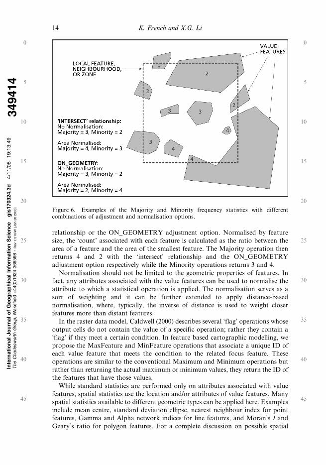
relationship or the ON_GEOMETRY adjustment option. Normalised by feature

size, the ‘count’ associated with each feature is calculated as the ratio between the

area of a feature and the area of the smallest feature. The Majority operation then

returns 4 and 2 with the ‘intersect’ relationship and the ON_GEOMETRY

adjustment option respectively while the Minority operations returns 3 and 4.

Normalisation should not be limited to the geometric properties of features. In

fact, any attributes associated with the value features can be used to normalise the

attribute to which a statistical operation is applied. The normalisation serves as a

sort of weighting and it can be further extended to apply distance-based

normalisation, where, typically, the inverse of distance is used to weight closer

features more than distant features.

In the raster data model, Caldwell (2000) describes several ‘flag’ operations whose

output cells do not contain the value of a specific operation; rather they contain a

‘flag’ if they meet a certain condition. In feature based cartographic modelling, we

propose the MaxFeature and MinFeature operations that associate a unique ID of

each value feature that meets the condition to the related focus feature. These

operations are similar to the conventional Maximum and Minimum operations but

rather than returning the actual maximum or minimum values, they return the ID of

the features that have those values.

While standard statistics are performed only on attributes associated with value

features, spatial statistics use the location and/or attributes of value features. Many

spatial statistics available to different geometric types can be applied here. Examples

include mean centre, standard deviation ellipse, nearest neighbour index for point

features, Gamma and Alpha network indices for line features, and Moran’s I and

Geary’s ratio for polygon features. For a complete discussion on possible spatial

Inte

rnati

on

al

Jo

urn

al

of

Geo

gra

ph

ical

Info

rmati

on

Scie

nce

gis

170324.3

d4/1

1/0

819:1

3:4

9T

he

Charlesw

ort

hG

roup,

Wakefield

+44(0

)1924

369598

-R

ev

7.5

1n/W

(Jan

20

2003)

349414

Figure 6. Examples of the Majority and Minority frequency statistics with differentcombinations of adjustment and normalisation options.


0

5

10

15

20

25

30

35

40

45

0

5

10

15

20

25

30

35

40

45

statistics in the vector data model, readers are referred to O’Sullivan and Unwin

(2003) and Wong and Lee (2005). Table 9 only lists two of them as examples. Instead

of applying spatial statistics to all the features on a vector layer, the VCM

framework limits the statistics to different spatial scopes of an operation, be it local,

focal, or zonal. Unlike standard statistics, outputs from spatial statistics vary. The

spatial statistics that calculate the mean centre of all the value points inside a zone

would create a new point. On the other hand, the statistics that calculate the

Moran’s I index for the value points inside a zone would only create a new attribute,

much like standard statistics.

4. A prototype syntax and its implementation

The previous sections discussed how the spatial scope of an operation could be

established with different feature types, how different types of feature selection and

geometry and attribute adjustments can be made to value features, and the set of

operations that can be carried out on these value features. Now, we tie all these

elements together into an operational framework and discuss some implementation

issues.

4.1 The prototype syntax

The proposed object-oriented syntax is:

NewLayer5FocusLayer.Operation (Scope, ValueLayer, Attribute, Adjustment,

Normalisation)

NewLayer is the newly created output layer where the results from an operation

are saved. As an alternative, this can be achieved by adding the results as a new

attribute to the focus layer, as the output layer and focus layer have the same set of

feature geometries.

FocusLayer is the layer from which the spatial scope of a local operation, the

neighbourhood of a focal operation, and the zone of a zonal operation are defined.

The focus layer is the layer where ‘irregular cells’, i.e. the spatial analysis unit of the

operation, is defined. Each feature in the focus layer has its own spatial scope. The

Operation is one of the conventional statistic operations or spatial statistic

operations listed in table 9 and discussed in section 3.

The Scope argument defines the scope of an operation based on the features in the

focus layer. This scope can be local, focal, or zonal in nature, as discussed in section

2. Some of the possible enumerations for the scope argument and their individual

parameters are listed in table 10. The ‘Local’ enumeration results in a local

operation; the chosen operations are performed only on those value features that

intersect the focus features themselves. There are no parameters. The ‘Zonal (String:

ZoneField)’ enumeration will put all focus features having the same attribute in the

given ZoneField as individual zones. If the ZoneField attribute is unique to each

feature, this zonal operation is essentially a local operation as discussed in section

2.3. Various classification methods could be used to group features on the focus

layer into zones before applying VCM operations. The remaining enumerations are

neighbourhoods for focal operations as discussed in section 2.2. Each has its own set

of parameters based on what type of neighbourhood it forms and from what type of

feature it is formed from.

Inte

rnati

on

al

Jo

urn

al

of

Geo

gra

ph

ical

Info

rmati

on

Scie

nce

gis

170324.3

d4/1

1/0

819:1

3:5

6T

he

Charlesw

ort

hG

roup,

Wakefield

+44(0

)1924

369598

-R

ev

7.5

1n/W

(Jan

20

2003)

349414


0

5

10

15

20

25

30

35

40

45

0

5

10

15

20

25

30

35

40

45

ValueLayer is the layer where statistics on feature attributes are calculated. Only

the value features that intersect the spatial scope of a focus feature, be it a local

feature, a neighbourhood, or a zone, are used in the calculation for the focus feature.

Since the spatial scopes of local and zonal operations are made of features from the

focus layer, it would be redundant to use the focus layer as the value layer in those

operations. Focal operations, on the other hand, often use the focus layer itself as

the value layer.

The Attribute argument indicates the attribute of value features on which statistics

are calculated. It can either be the name of an existing attribute or one of the

enumerations of the inherent geometric attributes such as LENGTH, DIRECTION,

ORIENTATION, and SINUOSITY for line features and PERIMETER and

AREA for polygon features. Table 9 lists the types of attributes associated with

some common operations.

The Adjustment argument is used to select a set of value features in the focus

feature, neighbourhood, and zone, and to adjust their geometries and attributes

before an operation is performed. The possible values are either a text string which

specifies a topological relationship or the enumerations of ON_GEOMETRY,

OVER_VALUE_FEATURE, and OVER_LNZ as discussed in section 2.4.

Finally, the Normalisation argument indicates a normalisation we wish to employ

on the chosen attribute as discussed in section 3. This argument can be ‘Geometry’,

indicating the attribute will be normalised by feature area or length, an attribute of

the value features, or ‘InverseDistance(Exponent)’, where Exponent indicates the

exponent applied to the distance. If this argument is omitted, no normalisation will

take place.

To better understand what exactly takes place during the execution of the

proposed syntax, the following pseudo code is provided to describe the logical flow

of VCM operations.

1. CREATE AN OUTPUT FEATURE LAYER WITH THE SAMEFEATURES AS IN THE FOCUS LAYER

2. ADD A NEW ATTRIBUTE TO THE OUTPUT FEATURE LAYER

Inte

rnati

on

al

Jo

urn

al

of

Geo

gra

ph

ical

Info

rmati

on

Scie

nce

gis

170324.3

d4/1

1/0

819:1

3:5

7T

he

Charlesw

ort

hG

roup,

Wakefield

+44(0

)1924

369598

-R

ev

7.5

1n/W

(Jan

20

2003)

349414

Table 10. The enumerations and associated parameters for the scope argument in theproposed syntax. A ‘Y’ in one of the last three columns indicates that the particular scope canbe used with a focus feature of that type and an ‘N’ means the particular scope is notapplicable to the feature type. The PivoType type has three enumerations: UPPER_LEFT,

CENTRE_EDGE, and CENTROID. These are discussed in detail in section 2.

Enumeration Point Line Polygon

Local Y Y YZonal (String: ZoneField) Y Y YRadial (Double: MinAngle, MaxAngle, MinRadius,

MaxRadius; Double: Xoffset, Yoffset)Y N N

Rectangular (Double: Height, Width, RotationAngle;PivoType: PivotEnumeration; Double: Xoffset, Yoffset)

Y N N

NearestNeighbour (Integer: NumOfNeighbours; Double:MaxDistance)

Y N N

ProximalRegion Y Y YEuclideanBuffer (Double: MinDistance, MaxDistance) Y Y YConnectivity (Integer: Order; Boolean: Accumulative) N Y YNetworkBuffer (Double: MinDistance, MaxDistance) N Y NGeneric (String: NeighbourDefinitionFile) Y Y Y


0

5

10

15

20

25

30

35

40

45

0

5

10

15

20

25

30

35

40

45

3. FOR EACH FEATURE ON THE FOCUS LAYER DO

a. DETERMINE OPERATIONAL SPATIAL SCOPEb. DETERMINE VALUE FEATURES BASED ON THE SPATIAL

SCOPEc. MAKE ADJUSTMENTS IF NECESSARYd. NORMALISE THE ATTRIBUTE IF NECESSARYe. PERFORM THE OPERATIONf. ASSIGN OPERATION RESULT TO THE NEW ATTRIBUTE

OF THE CORRESPONDING FEATURE ON THE OUTPUTFEATURE LAYER

END FOR

4.2 A preliminary implementation

Some of the operations were implemented using Microsoft’s Visual Basic for

Applications (VBA) programming language with ESRI ArcObjects#. This was done

primarily to ensure the same results were achieved with VCM as were obtained using

conventional geographical information system (GIS) analysis functions. As the

examples in the next section will show, the results from VCM were comparable to

the results through conventional means and they were much easier to produce and

required fewer steps.

While most of the local and zonal operations were implemented with relative ease,

we only implemented a few of the neighbourhood types discussed above and a

selection of statistical operations. Figure 7 shows an example of the graphical user

interface in our current implementation. It performs a focal sum operation where

the neighbourhood is defined as a radial neighbourhood and the

OVER_VALUE_FEATURE adjustment is used. The relationship between theuser interface and the proposed object-oriented syntax is also illustrated in the

figure. The obstacle at this point to our implementation is to expand the system to

include all of the neighbourhoods discussed and to develop an interface where the

user can design custom neighbourhoods that are specific to a particular application.

It was realised during the implementation that the most efficient and desirableimplementation will require programming at a much lower level than the current

VBA and ArcObjects approach. Although the VBA scripting we used is adequate

for analyses on a small to medium dataset, it would need a compilable programming

language and the access to lower level GIS analysis functions than ArcObjects

provides to be adequate for analyses on large datasets.

5. Application examples

Now that the VCM framework has been established, a few application examples are

presented next to demonstrate its usefulness. The first example analyses the

population coverage of the tornado warning sirens installed in Douglas County,

Kansas (figure 8(a)). The objective is to determine the number of people who are

able to hear the warning sound in the event of a tornado. Using raster cartographic

modelling operations, this is accomplished by converting vector census block datainto a population-per-cell raster layer and then using the zonal sum operation to

calculate total population within siren zones. There are two potential problems with

this approach. First, it requires an extra step of converting the vector data into a

Inte

rnati

on

al

Jo

urn

al

of

Geo

gra

ph

ical

Info

rmati

on

Scie

nce

gis

170324.3

d4/1

1/0

819:1

3:5

7T

he

Charlesw

ort

hG

roup,

Wakefield

+44(0

)1924

369598

-R

ev

7.5

1n/W

(Jan

20

2003)

349414


0

5

10

15

20

25

30

35

40

45

0

5

10

15

20

25

30

35

40

45

raster format in order to use raster cartographic modelling operations. Second, the

census block data may be compromised in the vector-to-raster conversion. It is

possible that a small census polygon, although it has a large population, may be

eliminated completely during the conversion if the raster cell size is not chosencarefully. The results from the raster analysis may vary with different cell sizes.

The VCM operations proposed in this article work directly with vector data. First

we may wish to determine the number of people residing inside the audible region of

each of the sirens. This can be calculated using a focal operation with a radial

neighbourhood. Assuming the sirens offer 360u coverage, the starting and ending

angles of the radial neighbourhood are the same, which gives a complete circle. Since

we can make the assumption that the sound can be heard anywhere inside the

maximum range, the minimum radius parameter is 0. The maximum radius is the

range from manufacturer specification. The population living inside each siren’sneighbourhood (the audibility zone) can be calculated with the following command

in the proposed syntax:

NewLayer5Siren.Sum (Radial (0, 0, 0, X), CensusBlock, POP, OVER_VALUE_FEATURE).

NewLayer is the output layer and Siren is the focus layer that is used to create theradial neighbourhoods for each siren. Sum is the operation that summarises

population in census blocks. The Radial (0, 0, 0, X) argument limits the

Inte

rnati

on

al

Jo

urn

al

of

Geo

gra

ph

ical

Info

rmati

on

Scie

nce

gis

170324.3

d4/1

1/0

819:1

3:5

7T

he

Charlesw

ort

hG

roup,

Wakefield

+44(0

)1924

369598

-R

ev

7.5

1n/W

(Jan

20

2003)

349414

Figure 7. The graphical user interface in the current implementation which performing afocal sum operation where the neighbourhood is defined as a radial neighbourhood and theOVER_VALUE_FEATURE adjustment is used. The relationship between the user interfaceand the proposed object-oriented syntax is also illustrated.


0

5

10

15

20

25

30

35

40

45

0

5

10

15

20

25

30

35

40

45

summarisation to the neighbourhood. In this case we use a radial neighbourhood

where hmin50, hmax50, rmin50, rmax5X, where X is the manufacturer’s statedaudible range of the sirens. CensusBlock is the value layer from which the

population attribute is summarised and POP is the name of the field where the

population in each census block is stored in CensusBlock.

The enumeration OVER_VALUE_FEATURE indicates that whenever a census

block is only partially contained in a radial neighbourhood, it is clipped into the

neighbourhood and its population value will be adjusted based on the ratio between

the portion that is inside the radial neighbourhood and its original size. This

adjustment implies that the population within the census block is uniformly

distributed. Without any further ancillary data, this is a reasonable assumption we

can make. The normalisation argument is omitted as there is no normalisation needed.

The above vector cartographic modelling operation calculates the number ofpeople covered by each siren. However, as our goal is to determine the total

population covered by all the sirens, a different approach must be taken. The

problem of using a focal operation lies in the fact that the neighbourhoods may

overlap and thus people in those overlapped areas may be counted more than once.

This can be solved by creating zones of audibility and then using a zonal

operation. A zone of audibility is created by merging overlap buffers for the sirens

into one polygon (figure 8(b)). To count the people inside zones, the following zonal

operation would be performed:

NewLayer5SirenZone. Sum (Zonal(ID), CensusBlock, POP, OVER_VALUE_FEATURE).

Except for the focus layer and the scope arguments, all other arguments in this

zonal operation are the same as in the focal operation. SirenZone is the focus layer

Inte

rnati

on

al

Jo

urn

al

of

Geo

gra

ph

ical

Info

rmati

on

Scie

nce

gis

170324.3

d4/1

1/0

819:1

4:0

5T

he

Charlesw

ort

hG

roup,

Wakefield

+44(0

)1924

369598

-R

ev

7.5

1n/W

(Jan

20

2003)

349414

Figure 8. Tornado population coverage analysis in the Douglas County, Kansas usingvector cartographic modelling operations. (a) Population in census blocks and the audibilityzones of individual sirens. (b) Overlapping individual audibility zones are merged and used ina zonal sum operation.


0

5

10

15

20

25

30

35

40

45

0

5

10

15

20

25

30

35

40

45

on which zones are defined. The zones are defined using the ID attribute in the

SirenZone layer. Each unique value in the ID field represents a zone of audibility.

The operation will check each of the census block polygons that intersect with a

zone and summarise their population. Those blocks that do not lie completely inside

the zone will be adjusted accordingly. The above zonal operation could also be

replaced by a local operation, as each polygon on the SirenZone layer represents a

separate zone.

The tornado siren application is an example of operations where the adjustment is

made with relation to value features. The next example demonstrates making

adjustments with relation to focus features. In this example, the analysis tries to

estimate the precipitation within the sub-watersheds in an agricultural watershed in

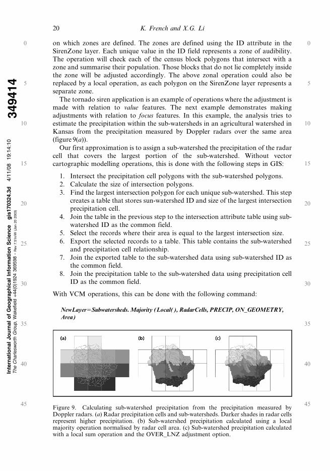
Kansas from the precipitation measured by Doppler radars over the same area(figure 9(a)).

Our first approximation is to assign a sub-watershed the precipitation of the radar

cell that covers the largest portion of the sub-watershed. Without vector

cartographic modelling operations, this is done with the following steps in GIS:

1. Intersect the precipitation cell polygons with the sub-watershed polygons.

2. Calculate the size of intersection polygons.

3. Find the largest intersection polygon for each unique sub-watershed. This step

creates a table that stores sun-watershed ID and size of the largest intersectionprecipitation cell.

4. Join the table in the previous step to the intersection attribute table using sub-

watershed ID as the common field.

5. Select the records where their area is equal to the largest intersection size.

6. Export the selected records to a table. This table contains the sub-watershed

and precipitation cell relationship.

7. Join the exported table to the sub-watershed data using sub-watershed ID as

the common field.

8. Join the precipitation table to the sub-watershed data using precipitation cell

ID as the common field.

With VCM operations, this can be done with the following command:

NewLayer5Subwatersheds. Majority (Local(), RadarCells, PRECIP, ON_GEOMETRY,Area)

Inte

rnati

on

al

Jo

urn

al

of

Geo

gra

ph

ical

Info

rmati

on

Scie

nce

gis

170324.3

d4/1

1/0

819:1

4:1

0T

he

Charlesw

ort

hG

roup,

Wakefield

+44(0

)1924

369598

-R

ev

7.5

1n/W

(Jan

20

2003)

349414

Figure 9. Calculating sub-watershed precipitation from the precipitation measured byDoppler radars. (a) Radar precipitation cells and sub-watersheds. Darker shades in radar cellsrepresent higher precipitation. (b) Sub-watershed precipitation calculated using a localmajority operation normalised by radar cell area. (c) Sub-watershed precipitation calculatedwith a local sum operation and the OVER_LNZ adjustment option.


0

5

10

15

20

25

30

35

40

45

0

5

10

15

20

25

30

35

40

45

In the command, NewLayer is the output, Majority is the operation,

Subwatersheds is the focus layer with all the sub-watersheds in the agricultural

watershed and Local() indicates we are performing these operations on the local

level. RadarCells is the value layer with precipitation measured at radar cells.

PRECIP is the attribute name in the RadarCells layer where precipitation is saved.

ON_GEOMETRY indicates that we wish to only consider the clipped portions of

the radar cells, but are making no adjustments to the precipitation data. Finally,

Area indicates that we wish to normalise the precipitation based on the area of the

intersecting radar cells. In this way, the radar cell that has the largest clipped area

inside the subwatershed will be given the most weight, and its value will be assigned

to the subwatershed focus feature. The result of this operation will produce a layer

of sub-watersheds each having the same value as the radar cell that covers the largest

portion of it (figure 9(b)).

Our second approximation, which is more accurate than the first one, takes into

account all the precipitation cells that intersect a sub-watershed. The precipitation in

a sub-watershed is calculated based on the proportion of the area that each

intersection precipitation cell has with the sub-watershed. With VCM operations,

this can be done with the following command:

NewLayer5Subwatersheds. Sum (Local(), RadarCells, PRECIP, OVER_LNZ)

Except for the operation, adjustment, and normalisation arguments, the above

command is the same as the one used in the first approximation. The SUM statistics

indicates that the sum of precipitation will be calculated for all the radar cells that

intersect a focus sub-watershed. The OVER_LNZ adjustment enumeration indicates

that the radar precipitation in a cell is adjusted based on the intersection between the

cell and the focus sub-watershed. No normalisation is required in this case because

the ratio of the area of intersection over the area of the entire subwatershed is

applied to the value. If a sub-watershed lies entirely in a single radar cell, it inherits

the precipitation value of that cell. If the sub-watershed lies across a number of

radar cells, its value will depend on the percentage of overlap of each cell and the

precipitation value of that cell. This result, as shown in figure 9(c), is more accurate

than the first approach, as it takes into account all available precipitation data over

the sub-watershed region.

In the tornado siren coverage example, population in a census block is the

summation of all the people living in the block. Thus, the population in a certain

portion of the census block depends on the size of the portion relative to the entire

block. Therefore, the adjustment used in the analysis is set to

OVER_VALUE_FEATURE. Precipitation amount, on the other hand, is uniform

over a radar cell. No matter which part of the cell intersects a sub-watershed, it has

the same precipitation amount. To calculate the precipitation in a sub-watershed,

the precipitation amount in each of intersection cells should be weighted based on

their overlapping sizes relative to the sub-watershed.

6. Comparison to raster cartographic modelling

One of the fundamental differences between the raster and vector data model lies in

the fact that in the vector data model there is no uniform spatial granule such as the

cell in the raster data model. A cell size has to be chosen in order to use raster

cartographic modelling operations. The spatial scope and the data used in an

Inte

rnati

on

al

Jo

urn

al

of

Geo

gra

ph

ical

Info

rmati

on

Scie

nce

gis

170324.3

d4/1

1/0

819:1

4:1

3T

he

Charlesw

ort

hG

roup,

Wakefield

+44(0

)1924

369598

-R

ev

7.5

1n/W

(Jan

20

2003)

349414


0

5

10

15

20

25

30

35

40

45

0

5

10

15

20

25

30

35

40

45

operation must be represented and approximated by the cells. In vector cartographic

modelling, the integrity of the focus features is not compromised by the cells as in

the raster data model. It eliminates forward and backward conversions between

vector and raster data and all the problems introduced by the conversions. One can

argue that, theoretically, the vector data model also has a resolution since any digital

computer is a finite system. However, this resolution is imposed by the limitation of

the digital computer and not by the analysis framework. Vector cartographic

modelling operations do not impose any arbitrary resolutions but simply maintain

the original resolution of the data through its analysis framework.

Another difference between the two frameworks comes from the fundamentally

different views adopted by the underlying data models. While the uniform spatial units

used in the raster data model empower the analysis on continuous fields and the

characterisation of spatial variations, they make it difficult in cases where a geographic

feature needs to be treated as a whole object. The position-oriented view inherent in the

raster data model limits its analyses to the cell level and hinders the analyses at the

feature level. Although the zonal operations in raster cartographic modelling alleviate

this problem to some degree by considering discrete features as zones, the framework

still has difficulty handling the neighbourhoods which are defined for individual

features or are based on the topological relationships between features (for example,

line connectivity and polygon adjacency). This difference also leads to the necessary

adjustments on feature attributes and geometry in the vector cartographic modelling

and new operations that deal with discrete features. Those adjustment options and new

operations are discussed in detail in section 2.4 and 3 respectively.

Just as the raster data model and the vector data model adopt a complementary

view to each other in modelling continuous phenomena and discrete features,

cartographic modelling operations in the raster and vector data model also

complement each other. The raster cartographic modelling framework is well suited

to the interpretation of location and the characterisation of spatial variation when

the spatial scope (for example, watershed and viewshed neighbourhoods) is

delineated from continuous surfaces or the data are derived from raster sources.

The vector cartographic modelling is more appropriate for characterising discrete

features and the relationships among the features.

7. Conclusions

This research extends the cartographic modelling framework to the vector data

model. It introduces local, focal, and zonal operations for point, line, and polygon

feature types. It proposes a prototype syntax and demonstrates the usefulness of

those operations with application examples. The fundamental difference between

the raster and vector data model leads to the new definitions of the spatial scopes of

locality, neighbourhoods, and zones, the adjustments on attributes and geometry,

the normalisation on attributes, and new operations.

The research provides a set of operations for the vector data model similar to

those available in the raster cartographic modelling framework. This similarity

makes possible spatial analysis in both data models in a similar style. It eliminates

forward and backward conversions between vector and raster data in order to use

raster cartographic modelling operations and all the problems introduced by the

conversions. It allows the use of neighbourhoods which are defined based on

topological relationships among features which may not be possible in the raster

data model.

Inte

rnati

on

al

Jo

urn

al

of

Geo

gra

ph

ical

Info

rmati

on

Scie

nce

gis

170324.3

d4/1

1/0

819:1

4:1

3T

he

Charlesw

ort

hG

roup,

Wakefield

+44(0

)1924

369598

-R

ev

7.5

1n/W

(Jan

20

2003)

349414


0

5

10

15

20

25

30

35

40

45

0

5

10

15

20

25

30

35

40

45

All the operations discussed in this research can be achieved through the use of

existing vector GIS analysis functions. No new functions are invented. The proposed

VCM framework, however, provides a set of higher level vector analysis operations

than the existing low-level vector analysis functions such as buffer and overlay

available in most vector GIS. Those high-level operations simplify spatial analysis

by reducing the number of required steps in the analysis as demonstrated in the

examples. In addition, using high-level operations could be more efficient than using

low-level GIS functions as intermediate file I/Os (required for storing intermediate

vector layers) can be reduced or omitted.

The proposed framework only considers the three simplest vector feature types i.e.

points, lines, and polygons, in the vector data model. It does not directly operate on

complex vector features built on linear reference systems. Also, the proposed

operations are only partially implemented at present. We plan to continue

implementing the operations and test them in various GIS applications. Another

missing component in the research is the lack of formality in the proposed prototype

syntax. Takeyama and Couclelis (1997) provided a comprehensive and rigid

formalisation on cartographic modelling operations under the name of Geo-

Algebra. It will be interesting to examine whether or not the proposed syntax can fit

into Geo-Algebra formalisation.

Although the raster cartographic modelling framework is a powerful spatial

analysis tool and remains widely used to date, we recognise that the operations are

not a set of atomic operations on which all the complex raster analysis can be based.

Also, the classification of the operations into local, focal and zonal groups is rather

arbitrary. For example, local operations can be considered as special focal

operations where the neighbourhood is a single cell and zonal operations are

special focal operations where the zone layer defines the neighbourhoods. While this

research focuses on proposing the corresponding operations in the vector data

model it does not examine the original cartographic modelling framework itself.

Although some important research has been done in this area, finding a general

framework for both raster and vector GIS operations remains a challenging research

topic (Chrisman 2002).

Acknowledgements

We sincerely thank Dr Dana Tomlin at the University of Pennsylvania, Dr Mike

Goodchild at the University of California at Santa Barbara, Dr Mike Hodgson at

the University of South Carolina, and four anonymous reviewers for providing

comments and suggestions that greatly improved the article.

ReferencesCALDWELL, D.R., 2000, Extending map algebra with flag operators. Available online at:

http://www.geocomputation.org/2000/GC007/Gc007.htm (accessed 15 August 2007).

CHAN, K. and WHITE, D., 1987, Map algebra: an object oriented implementation.

Proceedings, International Geographic Information Systems (IGIS) Symposium: The

Research Agenda, Vol. II, pp. 127–150 (Arlington, VA: Association of American

Geographers).

CHRISMAN, N., 2002, Exploring Geographic Information Systems (New York: John Wiley &

Sons).

CLEMENTINI, E., DI FELICE, P. and VAN OSSTROM, P., 1993, A small set of formal topological

relationships suitable for end-user interaction. In Advances in Spatial Database—3rd

International Symposium on Large Spatial Databases, SSD ’93. Lecture Notes in

Inte

rnati

on

al

Jo

urn

al

of

Geo

gra

ph

ical

Info

rmati

on

Scie

nce

gis

170324.3

d4/1

1/0

819:1

4:1

3T

he

Charlesw

ort

hG

roup,

Wakefield

+44(0

)1924

369598

-R

ev

7.5

1n/W

(Jan

20

2003)

349414


0

5

10

15

20

25

30

35

40

45

0

5

10

15

20

25

30

35

40

45

Computer Science 692, D. Abel and B.C. Ooi (Eds), pp. 277–295 (New York:

Springer-Verlag).

EGENHOFER, M.J. and HERRING, J., 1991, Categorizing binary topological relationships

between regions, lines, and points in geographic databases. Technical Report,

Department of Surveying Engineering, University of Maine, Orono, ME, USA.

HAKLAY, M., 2004, Map Calculus in GIS: a proposal and demonstration. International

Journal of Geographical Information Science, 18(2), pp. 107–125.

HODGSON, M.E. and GAILE, G., 1999, A cartographic modeling approach for surface

orientation-related applications. Photogrammetric Engineering & Remote Sensing,

65(1), pp. 85–95.

LEDOUX, H. and GOLD, C., 2006, A Voronoi-based map algebra. In Progress in Spatial Data

Handling–12th International Symposium on Spatial Data Handling, pp. 117–131

(Berlin: Springer).

LI, X. and HODGSON, M.E., 2004, Vector field data model and operations. GIScience and

Remote Sensing, 41(1), pp. 1–24.

MENNIS, J. and HULTGREN, T., 2006, Intelligent dasymetric mapping and its application to

areal interpolation. Cartography and Geographic Information Science, 33(3), pp.

179–194.

MENNIS, J., VIGER, R. and TOMLIN, D., 2005, Cubic map algebra functions for spatio-

temporal analysis. Cartography and Geographic Information Science, 32(1), pp. 17–32.

O’SULLIVAN, D. and UNWIN, D.J., 2003, Geographic Information Analysis (Hoboken, NJ:

John Wiley & Sons).

SCOTT, M., 1999, The extension of cartographic modeling for volumetric geographic analysis.

Available online at: http://www.spatial.maine.edu/,onsrud/ucgis/testproc/scott_m/

scottm.html (accessed 8 February 2007).

TAKEYAMA, M. and COUCLELIS, H., 1997, Map dynamics: integrating cellular automata and

GIS through geo-algebra. International Journal of Geographical Information Systems,

11(1), pp. 73–91.

TOBLER, W., 1995, The resel-based GIS. International Journal of Geographical Information

Systems, 9(1), pp. 95–100.

TOMLIN, D., 1990, Geographic Information Systems and Cartographic Modeling (Englewood

Cliffs, NJ: Prentice Hall).

WANG, X. and PULLAR, D., 2005, Describing dynamic modeling for landscapes with vector

map algebra in GIS. Computers & Geosciences, 31(8), pp. 956–967.

WONG, D.W.S. and LEE, J., 2005, Statistical Analysis of Geographic Information with ArcView

GIS and ArcGIS (Hoboken, NJ: John Wiley & Sons).

Inte

rnati

on

al

Jo

urn

al

of

Geo

gra

ph

ical

Info

rmati

on

Scie

nce

gis

170324.3

d4/1

1/0

819:1

4:1

3T

he

Charlesw

ort

hG

roup,

Wakefield

+44(0

)1924

369598

-R

ev

7.5

1n/W

(Jan

20

2003)

349414

24 Feature-based cartographic modelling

0

5

10

15

20

25

30

35

40

45

0

5

10

15

20

25

30

35

40

45

Documents

Research Article Feature-based cartographic modelling